Embed Size (px)
Citation preview

Group Theory Notes
0
1
2
3
4
5
6
7
Donald L. Kreher
December 21, 2012

ii

Ackowledgements
I thank the following people for their help in note taking and proof reading: Mark Gockenbach, KayleeWalsh.
iii

iv

Contents
Ackowledgements iii
1 Introduction 1
1.1 What is a group? . . . . . . . . . . . . . . . . . . . . . . . . . . . . . . . . . . . . . . . 1
1.1.1 Exercises . . . . . . . . . . . . . . . . . . . . . . . . . . . . . . . . . . . . . . . 2
1.2 Some properties are unique. . . . . . . . . . . . . . . . . . . . . . . . . . . . . . . . . . 3
1.2.1 Exercises . . . . . . . . . . . . . . . . . . . . . . . . . . . . . . . . . . . . . . . 5
1.3 When are two groups the same? . . . . . . . . . . . . . . . . . . . . . . . . . . . . . . . 6
1.3.1 Exercises . . . . . . . . . . . . . . . . . . . . . . . . . . . . . . . . . . . . . . . 7
1.4 The automorphism group of a graph . . . . . . . . . . . . . . . . . . . . . . . . . . . . 8
1.4.1 One more example. . . . . . . . . . . . . . . . . . . . . . . . . . . . . . . . . . . 9
1.4.2 Exercises . . . . . . . . . . . . . . . . . . . . . . . . . . . . . . . . . . . . . . . 10
2 The Isomorphism Theorems 11
2.1 Subgroups . . . . . . . . . . . . . . . . . . . . . . . . . . . . . . . . . . . . . . . . . . . 11
2.1.1 Exercises . . . . . . . . . . . . . . . . . . . . . . . . . . . . . . . . . . . . . . . 12
2.2 Cosets . . . . . . . . . . . . . . . . . . . . . . . . . . . . . . . . . . . . . . . . . . . . . 13
2.2.1 Exercises . . . . . . . . . . . . . . . . . . . . . . . . . . . . . . . . . . . . . . . 14
2.3 Cyclic groups . . . . . . . . . . . . . . . . . . . . . . . . . . . . . . . . . . . . . . . . . 15
2.3.1 Exercises . . . . . . . . . . . . . . . . . . . . . . . . . . . . . . . . . . . . . . . 16
2.4 How many generators? . . . . . . . . . . . . . . . . . . . . . . . . . . . . . . . . . . . . 17
2.4.1 Exercises . . . . . . . . . . . . . . . . . . . . . . . . . . . . . . . . . . . . . . . 19
2.5 Normal Subgroups . . . . . . . . . . . . . . . . . . . . . . . . . . . . . . . . . . . . . . 20
2.6 Laws . . . . . . . . . . . . . . . . . . . . . . . . . . . . . . . . . . . . . . . . . . . . . . 21
2.6.1 Exercises . . . . . . . . . . . . . . . . . . . . . . . . . . . . . . . . . . . . . . . 23
2.7 Conjugation . . . . . . . . . . . . . . . . . . . . . . . . . . . . . . . . . . . . . . . . . . 24
2.7.1 Exercises . . . . . . . . . . . . . . . . . . . . . . . . . . . . . . . . . . . . . . . 25
3 Permutations 27
3.1 Even and odd . . . . . . . . . . . . . . . . . . . . . . . . . . . . . . . . . . . . . . . . . 27
3.1.1 Exercises . . . . . . . . . . . . . . . . . . . . . . . . . . . . . . . . . . . . . . . 29
3.2 Group actions . . . . . . . . . . . . . . . . . . . . . . . . . . . . . . . . . . . . . . . . . 30
3.2.1 Exercises . . . . . . . . . . . . . . . . . . . . . . . . . . . . . . . . . . . . . . . 38
3.3 The Sylow theorems . . . . . . . . . . . . . . . . . . . . . . . . . . . . . . . . . . . . . 39
3.3.1 Exercises . . . . . . . . . . . . . . . . . . . . . . . . . . . . . . . . . . . . . . . 40
3.4 Some applications of the Sylow Theorems . . . . . . . . . . . . . . . . . . . . . . . . . 41
3.4.1 Exercises . . . . . . . . . . . . . . . . . . . . . . . . . . . . . . . . . . . . . . . 44
v

vi CONTENTS
4 Finitely generated abelian groups 454.1 The Basis Theorem . . . . . . . . . . . . . . . . . . . . . . . . . . . . . . . . . . . . . . 45
4.1.1 How many finite abelian groups are there? . . . . . . . . . . . . . . . . . . . . . 484.1.2 Exercises . . . . . . . . . . . . . . . . . . . . . . . . . . . . . . . . . . . . . . . 49
4.2 Generators and Relations . . . . . . . . . . . . . . . . . . . . . . . . . . . . . . . . . . 504.2.1 Exercises . . . . . . . . . . . . . . . . . . . . . . . . . . . . . . . . . . . . . . . 51
4.3 Smith Normal Form . . . . . . . . . . . . . . . . . . . . . . . . . . . . . . . . . . . . . 524.4 Applications . . . . . . . . . . . . . . . . . . . . . . . . . . . . . . . . . . . . . . . . . . 55
4.4.1 The fundamental theorem of finitely generated abelian groups . . . . . . . . . . 554.4.2 Systems of Diophantine Equations . . . . . . . . . . . . . . . . . . . . . . . . . 564.4.3 Exercises . . . . . . . . . . . . . . . . . . . . . . . . . . . . . . . . . . . . . . . 58
5 Fields 595.1 A glossary of algebraic systems . . . . . . . . . . . . . . . . . . . . . . . . . . . . . . . 595.2 Ideals . . . . . . . . . . . . . . . . . . . . . . . . . . . . . . . . . . . . . . . . . . . . . 605.3 The prime field . . . . . . . . . . . . . . . . . . . . . . . . . . . . . . . . . . . . . . . . 61
5.3.1 Exercises . . . . . . . . . . . . . . . . . . . . . . . . . . . . . . . . . . . . . . . 635.4 algebraic extensions . . . . . . . . . . . . . . . . . . . . . . . . . . . . . . . . . . . . . 645.5 Splitting fields . . . . . . . . . . . . . . . . . . . . . . . . . . . . . . . . . . . . . . . . 655.6 Galois fields . . . . . . . . . . . . . . . . . . . . . . . . . . . . . . . . . . . . . . . . . . 665.7 Constructing a finite field . . . . . . . . . . . . . . . . . . . . . . . . . . . . . . . . . . 66
5.7.1 Exercises . . . . . . . . . . . . . . . . . . . . . . . . . . . . . . . . . . . . . . . 67
6 Linear groups 696.1 The linear fractional group and PSL(2, q) . . . . . . . . . . . . . . . . . . . . . . . . . 69
6.1.1 Transitivity . . . . . . . . . . . . . . . . . . . . . . . . . . . . . . . . . . . . . . 736.1.2 The conjugacy classes . . . . . . . . . . . . . . . . . . . . . . . . . . . . . . . . 766.1.3 The permutation character . . . . . . . . . . . . . . . . . . . . . . . . . . . . . 826.1.4 Exercises . . . . . . . . . . . . . . . . . . . . . . . . . . . . . . . . . . . . . . . 83

Chapter 1
Introduction
1.1 What is a group?
Definition 1.1: If G is a nonempty set, a binary operation µ on G is a function µ : G×G→ G.
For example + is a binary operation defined on the integers Z. Instead of writing +(3, 5) = 8 we insteadwrite 3 + 5 = 8. Indeed the binary operation µ is usually thought of as multiplication and instead of µ(a, b)we use notation such as ab, a+ b, a b and a ∗ b. If the set G is a finite set of n elements we can present thebinary operation, say ∗, by an n by n array called the multiplication table. If a, b ∈ G, then the (a, b)–entryof this table is a ∗ b.
Here is an example of a multiplication table for a binary operation ∗ on the set G = a, b, c, d.
∗ a b c da a b c ab a c d dc a b d cd d a c b
Note that (a ∗ b) ∗ c = b ∗ c = d but a ∗ (b ∗ c) = a ∗ d = a.
Definition 1.2: A binary operation ∗ on set G is associative if
(a ∗ b) ∗ c = a ∗ (b ∗ c)
for all a, b, c ∈ G.
Subtraction − on Z is not an associative binary operation, but addition + is. Other examples of associativebinary operations are matrix multiplication and function composition.
A set G with a associative binary operation ∗ is called a semigroup. The most important semigroups aregroups.
Definition 1.3: A group is a set G with a special element e on which an associative binary operation∗ is defined that satisfies:
1. e ∗ a = a for all a ∈ G;
2. for every a ∈ G, there is an element b ∈ G such that b ∗ a = e.
1
2 CHAPTER 1. INTRODUCTION
Example 1.1: Some examples of groups.
1. The integers Z under addition +.
2. The set GL2(R) of 2 by 2 invertible matrices over the reals with matrix multiplication as the binaryoperation. This is the general linear group of 2 by 2 matrices over the reals R.
3. The set of matrices
G =
e =
[1 00 1
]
, a =
[−1 00 1
]
, b =
[1 00 −1
]
, c =
[−1 00 −1
]
under matrix multiplication. The multiplication table for this group is:
∗ e a b ce e a b ca a e c bb b c e ac c b a e
4. The non-zero complex numbers C is a group under multiplication.
5. The set of complex numbers G = 1, i,−1,−i under multiplication. The multiplication table for thisgroup is:
∗ 1 i −1 −i1 1 i −1 −ii i −1 −i 1−1 −1 −i 1 i−i −i 1 i −1
6. The set Sym (X) of one to one and onto functions on the n-element set X , with multiplication definedto be composition of functions. (The elements of Sym (X) are called permutations and Sym (X) iscalled the symmetric group on X . This group will be discussed in more detail later. If α,∈ Sym (X),then we define the image of x under α to be xα. If α, β ∈ Sym (X), then the image of x under thecomposition αβ is xαβ = (xα)β .)
1.1.1 Exercises
1. For each fixed integer n > 0, prove that Zn, the set of integers modulo n is a group under +, whereone defines a+ b = a+ b. (The elements of Zn are the congruence classes a, a ∈ Z.. The congruenceclass a is
x ∈ Z : x ≡ a (modn) = a+ kn : k ∈ Z.Be sure to show that this addition is well defined. Conclude that for every integer n > 0 there is agroup with n elements.
2. Let G be the subset of complex numbers of the form e2kπn
i, k ∈ Z. Show that G is a group undermultiplication. How many elements does G have?

1.2. SOME PROPERTIES ARE UNIQUE. 3
1.2 Some properties are unique.
Lemma 1.2.1 If G is a group and a ∈ G, then a ∗ a = a implies a = e.
Proof. Suppose a ∈ G satisfies a ∗ a = a and let b ∈ G be such that b ∗ a = e. Then b ∗ (a ∗ a) = b ∗ a andthus
a = e ∗ a = (b ∗ a) ∗ a = b ∗ (a ∗ a) = b ∗ a = e
Lemma 1.2.2 In a group G
(i) if b ∗ a = e, then a ∗ b = e and
(ii) a ∗ e = a for all a ∈ G
Furthermore, there is only one element e ∈ G satisfying (ii) and for all a ∈ G, there is only one b ∈ Gsatisfying b ∗ a = e.
Proof. Suppose b ∗ a = e, then
(a ∗ b) ∗ (a ∗ b) = a ∗ (b ∗ a) ∗ b = a ∗ e ∗ b = a ∗ b.
Therefore by Lemma 1.2.1 a ∗ b = e.Suppose a ∈ G and let b ∈ G be such that b ∗ a = e. Then by (i)
a ∗ e = a ∗ (b ∗ a) = (a ∗ b) ∗ a = e ∗ a = a
Now we show uniqueness. Suppose that a ∗ e = a and a ∗ f = a for all a ∈ G. Then
(e ∗ f) ∗ (e ∗ f) = e ∗ (f ∗ e) ∗ f = e ∗ f ∗ e = e ∗ f
Therefore by Lemma 1.2.1 e ∗ f = e. Consequently
f ∗ f = (f ∗ e) ∗ (f ∗ e) = f ∗ (e ∗ f) ∗ e = f ∗ e ∗ e = f ∗ e = f
and therefore by Lemma 1.2.1 f = e. Finally suppose b1 ∗ a = e and b2 ∗ a = e. Then by (i) and (ii)
b1 = b1 ∗ e = b1 ∗ (a ∗ b2) = (b1 ∗ a) ∗ b2 = e ∗ b2 = b2
Definition 1.4: Let G be a group. The unique element e ∈ G satisfying e ∗ a = a for all a ∈ G iscalled the identity for the group G. If a ∈ G, the unique element b ∈ G such that b ∗ a = e is called theinverse of a and we denote it by b = a−1.
If n > 0 is an integer, we abbreviate a ∗ a ∗ a ∗ · · · ∗ a︸ ︷︷ ︸
n times
by an. Thus a−n = (a−1)n = a−1 ∗ a−1 ∗ a−1 ∗ · · · ∗ a−1︸ ︷︷ ︸
n timesLet G = g1, g2, . . . , gn be a group with multiplication ∗ and consider the multiplication table of G.

4 CHAPTER 1. INTRODUCTION
gj
gi
gi ∗ gj
Let [x1 x2 x3 · · · xn] be the row labeled by gi in the multiplication table. I.e. xj = gi ∗ gj . If xj1 = xj2 ,then gi ∗ gj1 = gi ∗ gj2 . Now multiplying by g−1
i on the left we see that gj1 = gj2 . Consequently j1 = j2.Therefore
every row of the multiplication table contains every element of G exactly once
a similar argument shows that
every column of the multiplication table contains every element of G exactly once
A table satisfying these two properties is called a Latin Square.
Definition 1.5: A latin square of side n is an n by n array in which each cell contains a single elementform an n-element set S = s1, s2, . . . , sn, such that each element occurs in each row exactly once. Itis in standard form with respect to the sequence s1, s2, . . . , sn if the elements in the first row and firstcolumn are occur in the order of this sequence.
The multiplication table of a group G = e, g1, g2, . . . , gn−1 is a latin square of side n in standard formwith respect to the sequence
e, g1, g2, . . . , gn−1.
The converse is not true. That is not every latin square in standard form is the multiplication table of agroup. This is because the multiplication represented by a latin square need not be associative.
Example 1.2: A latin square of side 6 in standard form with respect to the sequence e, g1, g2, g3, g4, g5.
e g1 g2 g3 g4 g5g1 e g3 g4 g5 g2g2 g3 e g5 g1 g4g3 g4 g5 e g2 g1g4 g5 g1 g2 e g3g5 g2 g4 g1 g3 e
The above latin square is not the multiplication table of a group, because for this square:
(g1 ∗ g2) ∗ g3 = g3 ∗ g3 = e
but
g1 ∗ (g2 ∗ g3) = g1 ∗ g5 = g2
1.2. SOME PROPERTIES ARE UNIQUE. 5
1.2.1 Exercises
1. Find all Latin squares of side 4 in standard form with respect to the sequence 1, 2, 3, 4. For each squarefound determine whether or not it is the multiplication table of a group.
2. If G is a finite group, prove that, given x ∈ G, that there is a positive integer n such that xn = e. Thesmallest such integer is called the order of x and we write |x| = n.
3. Let G be a finite set and let ∗ be an associative binary operation on G satisfying for all a, b, c ∈ G
(i) if a ∗ b = a ∗ c, then b = c; and
(ii) if b ∗ a = c ∗ a, then b = c.
Then G must be a group under ∗ (Also provide a counter example that shows that this is false if G isinfinite.)
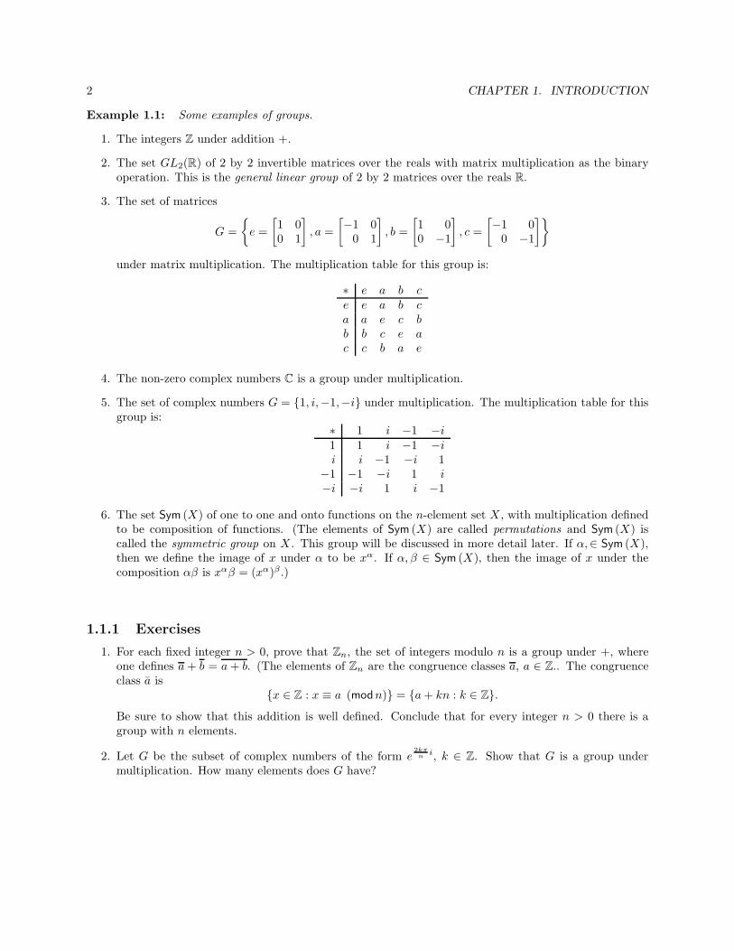
4. Show that the Latin Squaree g1 g2 g3 g4 g5 g6g1 e g3 g5 g6 g2 g4g2 g3 e g4 g1 g6 g5g3 g2 g1 g6 g5 g4 eg4 g5 g6 g2 e g3 g1g5 g6 g4 e g2 g1 g3g6 g4 g5 g1 g3 e g2
is not the multiplication table of a group.
5. Definition 1.6: A group G is abelian if a ∗ b = b ∗ a for all elements a, b ∈ G.
(a) Let G be a group in which the square of every element is the identity. Show that G is abelian.
(b) Prove that a groupG is abelian if and only if f : G→ G defined by f(x) = x−1 is a homomorphism.

6 CHAPTER 1. INTRODUCTION
1.3 When are two groups the same?
When ever one studies a mathematical object it is important to know when two representations of thatobject are the same or are different. For example consider the following two groups of order 8.
G =
g1 =
[1 00 1
]
, g2 =
[0 −11 0
]
, g3 =
[−1 00 −1
]
, g4 =
[0 1−1 0
]
,
g5 =
[1 00 −1
]
, g6 =
[−1 00 1
]
, g7 =
[0 11 0
]
, g8 =
[0 −1−1 0
]
G is a group of 2 by 2 matrices under matrix multiplication.
H =
h1 : x 7→ x, h2 : x 7→ ix, h3 : x 7→ −x, h4 : x 7→ −ix,h5 : x 7→ x, h6 : x 7→ −x, h7 : x 7→ ix, h8 : x 7→ −ix
H is a group complex functions under function composition. Here i =√−1 and a+ bi = a− bi.
The multiplication tables for G and H respectively are:
g1 g2 g3 g4 g5 g6 g7 g8g1 g1 g2 g3 g4 g5 g6 g7 g8g2 g2 g3 g4 g1 g7 g8 g6 g5g3 g3 g4 g1 g2 g6 g5 g8 g7g4 g4 g1 g2 g3 g8 g7 g5 g6
g5 g5 g8 g6 g7 g1 g3 g4 g2g6 g6 g7 g5 g8 g3 g1 g2 g4g7 g7 g5 g8 g6 g2 g4 g1 g3g8 g8 g6 g7 g5 g4 g2 g3 g1
h1 h2 h3 h4 h5 h6 h7 h8h1 h1 h2 h3 h4 h5 h6 h7 h8h2 h2 h3 h4 h1 h7 h8 h6 h5h3 h3 h4 h1 h2 h6 h5 h8 h7h4 h4 h1 h2 h3 h8 h7 h5 h6
h5 h5 h8 h6 h7 h1 h3 h4 h2h6 h6 h7 h5 h8 h3 h1 h2 h4h7 h7 h5 h8 h6 h2 h4 h1 h3h8 h8 h6 h7 h5 h4 h2 h3 h1
Observe that these two tables are the same except that different names were chosen. That is the one to onecorrespondence given by:
x g1 g2 g3 g4 g5 g6 g7 g8θ(x) h1 h2 h3 h4 h5 h6 h7 h8
carries the entries in the table for G to the entries in the table for H . More precisely we have the followingdefinition.
Definition 1.7: Two groups G and H are said to be isomorphic if there is a one to one correspondenceθ : H → G such that
θ(g1g2) = θ(g1)θ(g2)
for all g1, g2 ∈ G. The mapping θ is called an isomorphism and we say that G is isomorphic to H . Thislast statement is abbreviated by G ∼= H .If θ satisfies the above property but is not a one to one correspondence, we say θ is homomorphism. Thesewill be discussed later.
A geometric description of these two groups may also be given. Consider the square drawn in the
[xy
]
–plane with vertices the vectors in the set: V =
[10
]
,
[01
]
,
[−10
]
,
[0−1
]
.
y
x
[
0
1
]
[
1
0
]
[
−1
0
]
[
0
−1
]

1.3. WHEN ARE TWO GROUPS THE SAME? 7
The set of 2 by 2 matrices that preserve this set of vertices is the the group G. Thus G is the group ofsymmetries of the square.
Now consider the square drawn in the complex–plane with vertices the complexnumbers in the set: V = 1, i,−1,−i. The set of complex functions thatpreserve this set of vertices is the the group H . Thus H is also the group ofsymmetries of the square. Consequently it is easy to see that these two groupsare isomorphic.
ℑ
ℜ
i
1
−1
−i
1.3.1 Exercises
1. The groups given in example 1.1.3 and 1.1.5 are nonisomorphic.
2. The groups given in example 1.1.5 and Z4 are isomorphic.
3. Symmetries of the hexagon
(a) Determine the group of symmetries of the hexagon as a group G of two by two matrices. Writeout multiplication table of G.
(b) Determine the group of symmetries of the hexagon as a group H of complex functions. Write outthe multiplication table of H .
(c) Show explicitly that there is an isomorphism θ : G→ H .

8 CHAPTER 1. INTRODUCTION
1
2
3
4
5
6 ab
c
de
f
Γ1 = (V1, E1) Γ2 = (V2, E2)
Figure 1.1: Two isomorphic graphs.
1.4 The automorphism group of a graph
For another example of what is meant when two mathematical objects are the same consider the graph.
Definition 1.8: A graph is a pair Γ = (V , E) where
1. V is a finite set of vertices and
2. E is collection of unordered pairs of vertices called edges .
If a, b is an edge we say that a is adjacent to b. Notice that adjacent to is a symmetric relation on thevertex set V . Thus we also write a adj b for a, b ∈ EExample 1.3: A graph.
V = 1, 2, 3, 4E = 1, 2, 2, 3, 3, 4, 1, 4, 1, 3
In the adjacent diagram the vertices are represented by dots and an edgea, b is represented by drawing a line connecting the vertex labeled by ato the vertex labeled by b.
1 2
34
In figure 1.1 are two graphs Γ1 and Γ2.A careful scrutiny of the diagrams will reveal that they are the same as graphs. Indeed if we rename the
vertices of G1 with the function θ given by
x 1 2 3 4 5 6θ(x) b c d e a f
The resulting graph contains the same edges as G2. This θ is a graph isomorphism from Γ1 to Γ2. It is aone to one correspondence of the vertices that preserves that graphs structure.
Definition 1.9: Two graphs Γ1 = (V1, E1) and Γ2 = (V2, E2) are isomorphic graphs if there is a one toone correspondence θ : V1 → V2 such that
a adj b if and only if θ(a) adj θ(b)
Notice the similarity between definitions 1.7 and 1.9.
Definition 1.10: A one to one correspondence from a set X to itself is called a permutation on X .The set of all permutations on X is a group called the symmetric group and is denoted by Sym (X).
The automorphism group of a graph Γ = (V , E) is that set of all permutations on V that fix as a set theedges E .

1.4. THE AUTOMORPHISM GROUP OF A GRAPH 9
1.4.1 One more example.
Definition 1.11: The set of isomorphisms from a graph Γ = (V , E) to itself is called the automorphismgroup of Γ. We denote this set of mappings by Aut (Γ).
Before proceeding with an example let us make some notational conventions. Consider the one to onecorrespondence θ : x→ xθ given by
x 1 2 3 4 5 6 7 8 9 10 11
xθ 11 2 4 1 6 5 8 9 7 10 3
A simpler way to write θ is:
θ =
(1 2 3 4 5 6 7 8 9 10 1111 2 4 1 6 5 8 9 7 10 3
)
The image of x under θ is written in the bottom row. below x in the top row. Although this is simple aneven simpler notation is cycle notation. The cycle notation for θ is
θ = (1, 11, 3, 4)(2)(5, 6)(7, 8, 9)(10)
To see how this notation works we draw the diagram for the graph with edges: x, xθ for each x. Butinstead of drawing a line from x to xθ we draw a directed arc: x→ θ(x).
1
4 3
11
2
5
6 9
7
8
10
The resulting graph is a union of directed cycles. A sequence of vertices enclosed between parentheses in thecycle notation for the permutation θ is called a cycle of θ. In the above example the cycles are:
(1, 11, 3, 4), (2), (5, 6), (7, 8, 9), (10).
If the number of vertices is understood the convention is to not write the cycles of length one. (Cycles oflength one are called fixed points . In our example 2 and 10 are fixed points.) Thus we write for θ
θ = (1, 11, 3, 4)(5, 6)(7, 8, 9)
Now we are in good shape to give the example. The automorphism group of Γ1 in figure 1.1 is
Aut (Γ1) =
e, (1, 2), (5, 6), (1, 2)(5, 6), (1, 5)(2, 6)(3, 4),(1, 6)(2, 5)(3, 4), (1, 5, 2, 6)(3, 4), (1, 6, 2, 5)(3, 4)
e is used above to denote the identity permutation.The product of two permuations α and β is function composition read from left to right. Thus
xαβ = (xα)β
For example(1, 2, 3, 4)(5, 6) (1, 2, 3, 4, 5) = (1, 3, 5, 6)(2, 4)
as illustrated in Figure 1.2.

10 CHAPTER 1. INTRODUCTION
6
5
4
3
2
1
6
5
4
3
2
1
6
5
4
3
2
1
α β
αβ
Figure 1.2: The product of permutations α and β.
1.4.2 Exercises
1. Write the permutation that results from the product
(1 2 3 4 5 6 7 8 9 10 1111 2 4 1 6 5 8 9 7 10 3
)(1 2 3 4 5 6 7 8 9 10 113 6 4 11 9 7 8 10 5 2 1
)
in cycle notation.
2. Show that Aut (Γ1) is isomorphic to the group of symmetries of the square given in Section 1.3.
3. What is the automorphism group of the graph Γ = (V , E) for which
V = 1, 2, 3, 4, 5, 6; andE = 1, 2, 2, 3, 1, 3, 4, 5, 4, 6, 5, 6, 1, 4, 2, 5, 3, 6

Chapter 2
The Isomorphism Theorems
Through out the remainder of the text we will use ab to denote the product of group elements a and b andwe will denote the identity by 1.
2.1 Subgroups
Definition 2.1: A nonempty subset S of the group G is a subgroup of G if S a group under binaryoperation of G. We use the notation S ≤ G to indicate that S is a subgroup of G.
If S is a subgroup we see from Lemma 1.2.1 that 1 the identity for G is also the identity for S. Conse-quently the following theorem is obvious:
Theorem 2.1.1 A subset S of the group G is a subgroup of Gif and only if
(i) 1 ∈ S;
(ii) a ∈ S ⇒ a−1 ∈ S;
(iii) a, b ∈ S ⇒ ab ∈ S.
Although the above theorem is obvious it shows what must be checked to see if a subset is a subgroup.This checking is simplified by the next two theorems.
Theorem 2.1.2 If S is a subset of the group G, then S is a subgroup of G if and only if S is nonempty andwhenever a, b ∈ S, then ab−1 ∈ S.
Proof. If S is a subgroup, then of course S is nonempty and whenever a, b ∈ S, then ab−1 ∈ S.Conversely suppose S is a nonempty subset of the Group G such that whenever a, b ∈ S, then ab−1 ∈ S.
We use Theorem 2.1.1. Let a ∈ S, then 1 = aa−1 ∈ S and so a−1 = 1a−1 ∈ S. finally, if a, b ∈ S, thenb−1 ∈ S by the above and so ab = a(b−1)−1 ∈ S.
Theorem 2.1.3 If S is a subset of the finite group G, then S is a subgroup of G if and only if S is nonemptyand whenever a, b ∈ S, then ab ∈ S.
11

12 CHAPTER 2. THE ISOMORPHISM THEOREMS
Proof. If S is a subgroup, then obviously S is nonempty and whenever a, b ∈ S, then ab ∈ S.Conversely suppose S is nonempty and whenever a, b ∈ S, then ab ∈ S. Then let a ∈ S. The above
property says that a2 = aa ∈ S and so a3 = aa2 ∈ S and so a4 = aa3 ∈ S and so on and on and on. That isan ∈ S for all integers n > 0. But G is finite and thus so is S. Consequently the sequence,
a, a2, a3, a4, a5, . . . , an, . . .
cannot continue to produce new elements. That is there must exist and m < n such that am = an. Thus1 = an−m ∈ S. Therefore for all a ∈ S, there is a smallest integer k > 0 such that ak = 1. moreover,a−1 = ak−1 ∈ S. finally if a, b ∈ S, then b−1 ∈ S by the above and so by the assumed property we haveab−1 ∈ S. Therefore by Theorem 2.1.2 we have that S is a subgroup as desired.
Example 2.1: Examples of subgroups.
1. Both 1 and G are subgroups of the group G. Any other subgroup is said to be a proper subgroup.The subgroup 1 consisting of the identity alone is often called the trivial subgroup.
2. If a is an element of the group G, then
〈a〉 = . . . , a−3, a−2, a−1, 1, a, a2, a3, a4, . . .
are all the powers of a. This is a subgroup and is called the cyclic subgroup generated by a.
3. If θ : G→ H is a homomorphism, then
kernel (θ) = x ∈ G : θx = 1
andimage (θ) = y ∈ H : θx = y for some x ∈ G
are subgroups of G and H respectively.
4. The group given in Example 1.1.3 is a subgroup of the group of matrices given in Section 1.3.
Theorem 2.1.4 Let X be a subset of the group G, then there is a smallest subgroup S of G that containsX. That is if T is any other subgroup containing X, then T ⊃ S.
Proof. Exercise 2.1.1
Definition 2.2: If X is a subset of the group G, then the smallest subgroup of G containing X isdenoted by 〈X〉 and is called the subgroup generated by X . We say that X generates 〈X〉
2.1.1 Exercises
1. Prove Theorem 2.1.4
2. If S and T are subgroups of the group G, then S ∩ T is a subgroup of G.

2.2. COSETS 13
2.2 Cosets
Definition 2.3: If S is a subgroup of G and a ∈ G, then
Sa = xa : x ∈ S
is a right coset of S.
If S is a subgroup of G and a ∈ G, then it is easy to see that Sa = Sb whenever b ∈ Sa. An elementb ∈ Sa is said to be a coset representative of the coset Sa.
Lemma 2.2.1 Let S be a subgroup of the group Gand let a, b ∈ G. Then Sa = Sb if and only if ab−1 ∈ S.
Proof. Suppose Sa = Sb. Then a ∈ Sa and so a ∈ Sb. Thus a = xb for some x ∈ S and we see thatab−1 = x ∈ S.
Conversely, suppose ab−1 ∈ S. Then ab−1 = x, for some x ∈ S. Thus a = xb and consequently Sa = Sxb.Observe that Sx = S because x ∈ S. Therefore Sa = Sb.
Lemma 2.2.2 Cosets are either identical or disjoint.
Proof. Let S be a subgroup of the group G and let a, b ∈ G. Suppose that Sa ∩ Sb 6= ∅. Then there is az ∈ Sa ∩ Sb. Hence we may write z = xa for some x ∈ S and z = yb for some y ∈ S. Thus, xa = by. Butthen ab−1 = yx−1 ∈ S, because x, y ∈ S and S is a subgroup.
Definition 2.4: The number of elements in the finite group G is called the order of G and is denotedby |G|.
If S is a subgroup of the finite group G it is easy to see that |Sa| = |S| for any coset Sa. Also becausecosets are identical or disjoint we can choose coset representatives a1, a2, . . . , ar so that
G = Sa1∪Sa2∪Sa3∪ · · · ∪Sar.Thus G can be written as the disjoint union of cosets and these cosets each have size |S|. The number r ofright cosets of S in G is denoted by |G : S| and is called the index of S in G. This discussion establishes thefollowing important result of Lagrange (1736-1813).
Theorem 2.2.3 (Lagrange) If S is a subgroup of the finite group G, then
|G : S| = |G||S|Thus the order of S divides the order of G.
Definition 2.5: If x ∈ G and G is finite, the order of x is |x| = | 〈x〉 |.
Corollary 2.2.4 If x ∈ G and G is finite, then |x| divides |G|.

14 CHAPTER 2. THE ISOMORPHISM THEOREMS
Proof. This is a direct consequence of Theorem 2.2.3.
Corollary 2.2.5 If |G| = p a prime, then G is cyclic.
Proof. Let x ∈ G, x 6= 1. Then |x| = p, because p is a prime. Hence < x >= G and therefore G is cyclic.
A useful formula is provided in the next theorem. If X and Y are subgroups of a group G, then we define
XY = xy : x ∈ X and y ∈ Y .
Lemma 2.2.6 (Product formula) If X and Y are subgroups of G, then
|X Y ||X ∩ Y | = |X ||Y |
Proof. We count pairs[(x, y), z)] (2.1)
such that xy = z, x ∈ X , y ∈ Y in two ways.First there are |X | choices for x and |Y | choices for y this determines z to be xy, and so there are |X ||Y |
pairs 2.1.Secondly there are |XY | choices for z. But given z ∈ XY there may be many ways to write z as z = xy,
where x ∈ X and y ∈Y Let z ∈ XY be given and write z = x2y2. If x ∈ X and y ∈ Y satisfy xy = z, then
x−1x2 = yy−12 ∈ X ∩ Y.
Conversely if a ∈ X ∩ Y , then because X ∩ Y is a subgroup of both X and Y , we see that x2a ∈ X anda−1y2 ∈ Y thus the ordered pair (x2a, a
−1y2) ∈ X×Y is such that (x2a)(a−1y2) = x2y2. Thus given z ∈ XY
the number of pairs (x, y) such that x ∈ X , y ∈ Y and xy = z is |X ∩ Y |. Thus there are |X ∩ Y ||XY |pairs 2.1.
2.2.1 Exercises
1. Let G = Sym (1, 2, 3, 4) and let H = 〈(1, 2, 3, 4), (2, 4)〉. Write out all the cosets of H in G.
2. Let |G| = 15. If G has only one subgroup of order 3 and only one subgroup of order 5, then G is cyclic.
3. Use Corollary 2.2.5 to show that the Latin square given in Exercise 1.2.1.4 cannot be the multiplicationtable of a group.
4. Recall that the determinant map δ : GLn(R) → R is a homomorphism. Let S = ker δ. Describe thecosets of S in GLn(R).

2.3. CYCLIC GROUPS 15
2.3 Cyclic groups
Among the first mathematics algorithms we learn is the division algorithm for integers. It says given aninteger m and an positive integer divisor d there exists a quotient q and a remainder r < d such thatm
d= q +
r
d. This is quite easy to prove and we encourage the reader to do so. Formally the division
algorithm is.
Lemma 2.3.1 (Division Algorithm) Given integers m and d > 0, there are uniquely determined integersd and r satisfying
m = dq + r
and
0 ≤ r < d
Proof. See exercise 1
Using the division algorithm we can establish some interesting results about cyclic groups. First recallthat G is cyclic group means that there is an a ∈ G such that
G = 〈a〉 = . . . , a−3, a−2, a−1, 1, a, a2, a3, a4, . . .
Theorem 2.3.2 Every subgroup of a cyclic group is cyclic.
Proof. Let G = 〈a〉 be a cyclic group and suppose H is a subgroup of G. If H = 1, then H = 〈1〉.Otherwise there is a smallest positive integer d such that ad ∈ H . We will show that H =
⟨ad⟩. Let h ∈ H .
Then h = am for some integer m. Applying Lemma 2.3.1, the division algorithm, we find integers q and rsuch that
m = dq + r
with 0 ≤ r < d. Then
h = am = adq+r = adqar = (ad)qar
Hence ar = (ad)−qh ∈ H . But 0 ≤ r < d, so r = 0, for otherwise we would contradict that d is the smallestpositive integer such that ad ∈ H Consequently, h = am = adq = (ad)q ∈
⟨ad⟩= H .
Theorem 2.3.3 Let G = 〈a〉 have order n. Then for each k dividing n, G has a unique subgroup of orderk, namely
⟨an/k
⟩.
Proof. First let t = nk . Then it is easy to see that 〈at〉 is a subgroup of order k. Let H be any subgroup
of G of order k. Then by the proof of Theorem 2.3.2 we have H =⟨ad⟩; where d is the smallest positive
integer such that ad ∈ H . We apply the division algorithm to obtain integers q and r so that
n = dq + r and 0 ≤ r < d
Thus 1 = an = adq+r = (ad)qar and therefore ar = (ad)−q ∈ H . Consequently, r = 0 and so n = dq. Alsok = |H | = | 〈at〉 | = q = n/d. Therefore d = n/k = t, i.e. H =
⟨ad⟩= 〈at〉.
16 CHAPTER 2. THE ISOMORPHISM THEOREMS
2.3.1 Exercises
1. Prove Lemma 2.3.1.
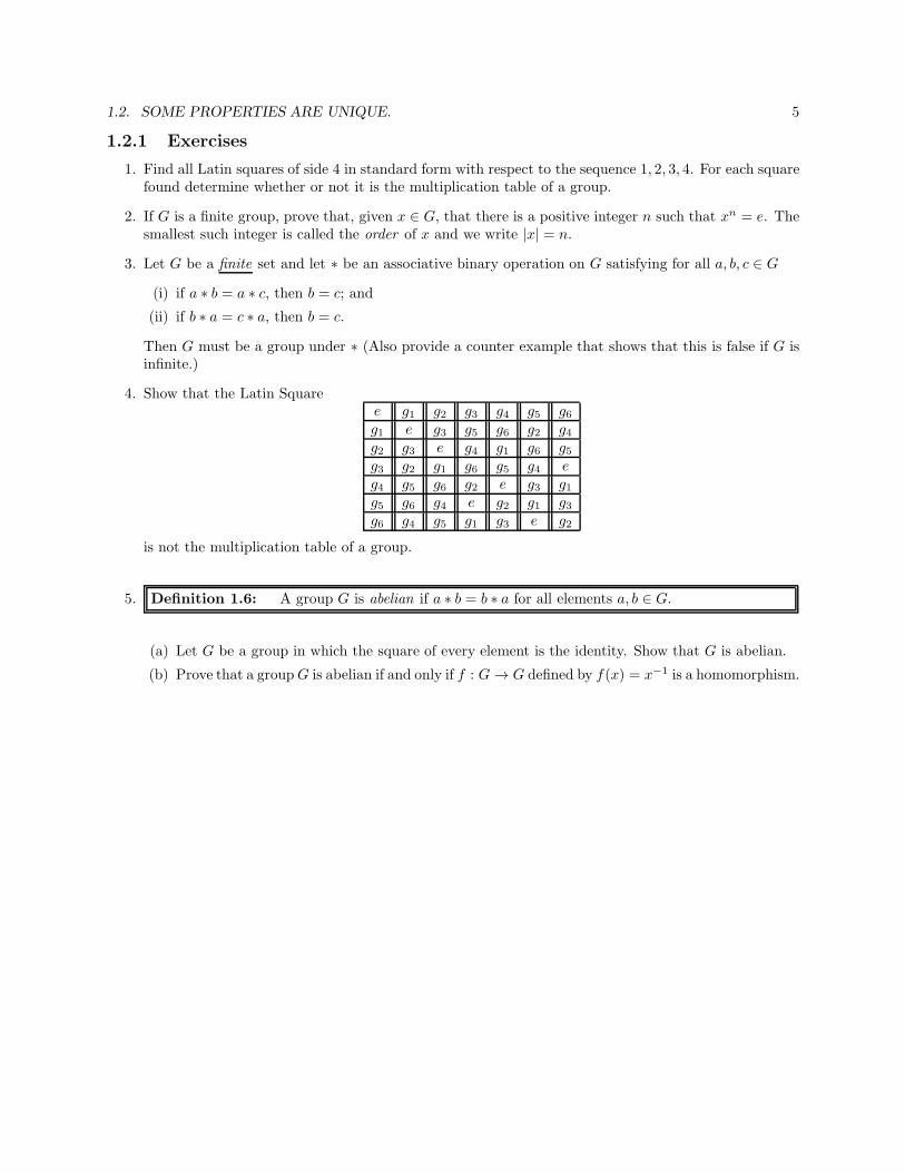
2. The subgroup lattice of a group is a diagram that illustrates the relationships between the varioussubgroups of the group. The diagram is a directed graph whose vertices are the the subgroups and anarc is drawn from a subgroup H to a subgroup K, if H is a maximal proper subgroup of K. The arc islabeled by the index |K : H |. Usually K is drawn closer to the top of the page, then H . For examplethe subgroup lattice of the cyclic group G = 〈a〉 of order 12 is
〈a〉
〈a3〉〈a2〉
〈a6〉〈a4〉
9
3 2
2 3
2 3
3
(a) Draw the subgroup lattice for a cyclic group of order 30.
(b) Draw the subgroup lattice for a cyclic group of order p2q; where p and q are distinct primes.
2.4. HOW MANY GENERATORS? 17
2.4 How many generators?
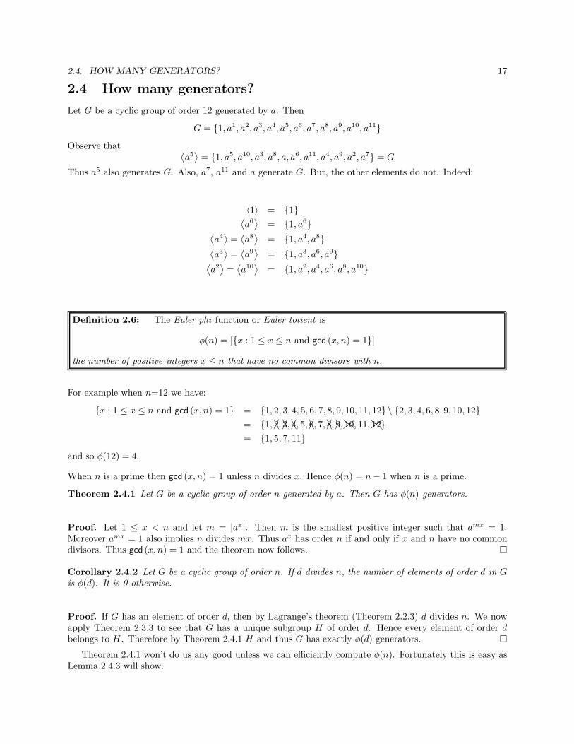
Let G be a cyclic group of order 12 generated by a. Then
G = 1, a1, a2, a3, a4, a5, a6, a7, a8, a9, a10, a11Observe that
⟨a5⟩= 1, a5, a10, a3, a8, a, a6, a11, a4, a9, a2, a7 = G
Thus a5 also generates G. Also, a7, a11 and a generate G. But, the other elements do not. Indeed:
〈1〉 = 1⟨a6⟩
= 1, a6⟨a4⟩=⟨a8⟩
= 1, a4, a8⟨a3⟩=⟨a9⟩
= 1, a3, a6, a9⟨a2⟩=⟨a10⟩
= 1, a2, a4, a6, a8, a10
Definition 2.6: The Euler phi function or Euler totient is
φ(n) = |x : 1 ≤ x ≤ n and gcd (x, n) = 1|
the number of positive integers x ≤ n that have no common divisors with n.
For example when n=12 we have:
x : 1 ≤ x ≤ n and gcd (x, n) = 1 = 1, 2, 3, 4, 5, 6, 7, 8, 9, 10, 11, 12 \ 2, 3, 4, 6, 8, 9, 10, 12= 1, 2, 3, 4, 5, 6, 7, 8, 9,❩❩10, 11,❩❩12= 1, 5, 7, 11
and so φ(12) = 4.
When n is a prime then gcd (x, n) = 1 unless n divides x. Hence φ(n) = n− 1 when n is a prime.
Theorem 2.4.1 Let G be a cyclic group of order n generated by a. Then G has φ(n) generators.
Proof. Let 1 ≤ x < n and let m = |ax|. Then m is the smallest positive integer such that amx = 1.Moreover amx = 1 also implies n divides mx. Thus ax has order n if and only if x and n have no commondivisors. Thus gcd (x, n) = 1 and the theorem now follows.
Corollary 2.4.2 Let G be a cyclic group of order n. If d divides n, the number of elements of order d in Gis φ(d). It is 0 otherwise.
Proof. If G has an element of order d, then by Lagrange’s theorem (Theorem 2.2.3) d divides n. We nowapply Theorem 2.3.3 to see that G has a unique subgroup H of order d. Hence every element of order dbelongs to H . Therefore by Theorem 2.4.1 H and thus G has exactly φ(d) generators.
Theorem 2.4.1 won’t do us any good unless we can efficiently compute φ(n). Fortunately this is easy asLemma 2.4.3 will show.

18 CHAPTER 2. THE ISOMORPHISM THEOREMS
Lemma 2.4.3
(i) φ(1) = 1;
(ii) if p is a prime, then φ(pa) = pa − pa−1; and
(iii) if gcd (m,n) = 1, then φ(mn) = φ(m)φ(n).
Proof.
(i) It is obvious that φ(1) = 1.
(ii) Observe that gcd (x, pa) 6= 1 if an only if p divides x. Thus crossing out every entry divisible by p fromthe pa−1 by p array
1 2 3 . . . p− 1 pp+ 1 p+ 2 p+ 3 . . . 2p− 1 2p2p+ 1 2p+ 2 2p+ 3 . . . 3p− 1 3p
......
(pa−1 − 1)p+ 1 (pa−1 − 1)p+ 2 (pa−1 − 1)p+ 3 . . . pa − 1 pa
delete the last column leaving an array of size pa−1 by p− 1.
Thus φ(n) = pa−1(p− 1) = pa − pa−1.
(iii) Let G be a cyclic group of order mn, where gcd (m,n) = 1. By the Euclidean algorithm there existsintegers a and b such that am+ bn = 1. (Note this means gcd (a, n) = gcd (b,m) = 1.)
If x ∈ G is a generator, then x has order mn and
x = x1 = xam+bn = (xm)a (xn)b = y z
Let y = (xm)a, then because gcd (a, n) = 1 and gcd (m,n) = 1 we see that |y| = n. Similarly z = (xn)b
has order m.
If x = y2z2 is also such that y2 has order m and z2 has order n. Then
yz = x = y2z2 ⇒ y−12 y = z2z
−1
Therefore, because multiplication in G is commutative we see that
(y−12 y)n = (z2z
−1)n = zn2 z−n = 1
and hence y = y2. Similarly z = z2.
Therefore x can be written uniquely as x = yz, where y ∈ G has order n and z ∈ G has order m. ByCorollary 2.4.2, we know G has exactly φ(mn) elements x of order mn, φ(n) elements y of order n andφ(m) elements z of order m. Consequently we may conclude
φ(mn) = φ(m)φ(n).

2.4. HOW MANY GENERATORS? 19
Example 2.2: Computing with the Euler phi function.
1. φ(40) = φ(2351) = φ(23)φ(51) = (23 − 22)(51 − 50) = (4)(4) = 16
2. φ(300) = φ(223152) = φ(23)φ(31)φ(52) = (22 − 21)(31 − 30)(52 − 51) = (3)(2)(20) = 120
3. φ(63) = φ(2333) = φ(23)φ(33) = (23 − 22)(33 − 32) = (4)(18) = 72
2.4.1 Exercises
1. How many generators does a cyclic group of order 400 have?
2. For each positive integer x, how elements of order x does a cyclic group of order 400 have?
3. For any positive integer n, we have∑
d|n φ(d) = n.
20 CHAPTER 2. THE ISOMORPHISM THEOREMS
2.5 Normal Subgroups
Definition 2.7: A subgroup N of the group G is a normal subgroup if g−1Ng = N for all g ∈ G. Weindicate that N is a normal subgroup of G with the notation N E G.
Example 2.3: Some normal subgroups
1. Every subgroup of an abelian group is a normal subgroup.
2. The subset of matrices of GL2(R) that have determinant 1 is a normal subgroup of GL2(R).
Lemma 2.5.1 The subgroup N of G is a normal subgroup of G if and only if g−1Ng ⊆ N for all g ∈ G.Proof. Suppose N is subgroup of G satisfying g−1Ng ⊆ N for all g ∈ G. Then for all n ∈ N and all g ∈ G,we have
gng−1 = (g−1)−1n(g−1) = n′ ∈ N
for some n′, because (g−1) ∈ G. Solving for n we find
n = g−1n′g ∈ g−1Ng.
Hence N ⊆ g−1Ng and so, N = g−1Ng. Therefore N is a normal subgroup of G.The converse is obvious.
The multiplication of two subsets A and B of the group G is defined by
AB = ab : a ∈ A and b ∈ B
This multiplication is associative because the multiplication in G is associative. Thus, if a collection of subsetsof G are carefully chosen, then it may be possible that they could form a group under this multiplication.
Theorem 2.5.2 If N is a normal subgroup of G, then the cosets of N form a group. If G is finite, thisgroup has order |G : N |.Proof. Let x, y ∈ G. Then
NxNy = NxNx−1xy = NNxy = Nxy
because N is normal in G. Thus the product of two cosets is a coset. It is easy to see N is the identity andNx−1 is (Nx)−1 for this multiplication. Thus the cosets form a group as claimed. Furthermore when G isfinite Theorem 2.2.3 applies and the number of cosets is |G : N |.
Definition 2.8: The group of cosets of a normal subgroup N of the group G is called the quotientgroup or the factor group of G by N . This group is denoted by G/N which is read “G modulo N” or “Gmod N”.
Notice how this definition closely follows what we already know as modular arithmetic. Indeed Zn (theintegers modulo n) is precisely the factor group Z/nZ.

2.6. LAWS 21
2.6 Laws
The most important elementary theorem of group theory is:
Theorem 2.6.1 (First law) Let θ : G→ H be a homomorphism. Then N = kernel (θ) is a normal subgroupof G and
G/N ∼= image (θ) .
Proof. In Example 2.1.3 we have already seen that N is a subgroup of G. To see that N is a normalsubgroup, let g ∈ G and n ∈ N . Then
θ(g−1ng) = θ(g−1)θ(n)θ(g) = θ(g−1)θ(g) = θ(g−1g) = θ(1) = 1.
Thus g−1ng ∈ N and hence by Lemma 2.5.1 N is normal in G.Now define Ψ : G/N → image (θ) by
Ψ(Ng) = θ(g).
To see that Ψ well defined suppose Nx = Ny. Then, xy−1 ∈ N . So, 1 = θ(xy−1) = θ(x)θ(y)−1. Thereforeθ(x) = θ(y) and hence Ψ(Nx) = Ψ(Ny).
Also, Ψ is a homomorphism, for
Ψ(NxNy) = Ψ(Nxy) = θ(xy) = θ(x)θ(y) = Ψ(Nx)Ψ(Ny).
Moreover Ψ is one to one since Ψ(Nx) = Ψ(Ny) implies θ(x) = θ(y). So, xy−1 ∈ kernel (θ) = N . But then,Nx = Ny. Clearly image (Ψ) = image (θ). Therefore Ψ is an isomorphism between G/N and image (θ).
Suppose K E G, and consider the mapping π : G → G/K defined by π(x) = Kx. Observe thatπ(xy) = Kxy = Kxky and
π(x) = K ⇔ Kx = K ⇔ x ∈ K.Thus π is a homomorphism with kernel K. The mapping π is called the natural map.
Theorem 2.6.2 If H ≤ G and N E G, then HN = NH is a subgroup of G.
Proof. Let S = 〈H,N〉 be that smallest subgroup of G that contains H and N . (I.e. S is the intersectionover all subgroups of G, that contain H and also N .) Certainly H,N ⊆ NH and HN,NH ⊆ S. Hence itsuffices to show that HN and NH are subgroups of G. If h1n1, h2n2 ∈ HN , then
(h1n1)(h2n2)−1 = h1(n1n
−12 h−1
2 ) = h1(h−12 n3) ∈ HN
for some n3 ∈ N , because N E G. Therefore by Theorem 2.1.2 HN is a subgroup. A similar argument willshow that NH is also a subgroup.
Remark: It follows from Theorem 2.6.2 and the product formula (Theorem 2.2.6) that if H ≤ G andN E G, then |NH |/|N | = |H |/|H ∩N |. This suggests the second isomorphism law.
Theorem 2.6.3 (Second law) Let H and N be subgroups of G with N normal. Then H ∩N is normal inH and H/(H ∩N) ∼= NH/N .
Proof. Let π : G → G/T be the natural map and let π↓H be the restriction of π to H . Because π↓H isa homomorphism with kernel H ∩ N we see by Theorem 2.6.1, that H ∩ N E H and that H/(H ∩ N) ∼=image (π↓H). But by the above remark we know that the image of π↓H is just the collection of cosets of Nwith representatives in H . These are the cosets of of N in HN/N .

22 CHAPTER 2. THE ISOMORPHISM THEOREMS
Theorem 2.6.4 (Third law) Let M ⊂ N be normal subgroups of G. Then N/M is a normal subgroup ofG/M and
(G/M)/(N/M) ∼= G/N
.
Proof. Define f : G/M → G/N by f(Mx) = Nx. Check that f is a well-defined homomorphism withkernel N/M and image G/N . Apply The First law.
The fourth law of isomorphism is the law of correspondence given in Theorem 2.6.5. If X and Y are anysets and f : X → Y is any onto function. then f defines a one-to-one correspondence between the all of thesubsets of Y and some of the subsets of X . Namely if S ⊆ X
f(S) = f(x) : x ∈ S ⊆ Yand if T ⊆ Y , then
f−1(T ) = x ∈ X : f(x) ∈ T .The Law of Correspondence is a group theoretic translation of these observation.
Theorem 2.6.5 (Law of correspondence) Let K E G and let π : G → G/K be the natural map. Thenπ defines a one-to-one correspondence between
A = A : K ≤ A ≤ G = all subgroups of G containing K
andB = B : B ≤ G/K = all subgroups of G/K
If the subgroup of G/K corresponding to A ≤ G is denoted by A, then
1. A = A/K = π(A);
2. K ≤ A1 ≤ A2 ≤ G⇔ A1 ≤ A2, and then |A2 : A1| = |A2 : A1|;3. K ≤ A1 E A2 ≤ G⇔ A1 E A2, and then A2/A1
∼= A2/A1.
Proof. First we show that the correspondence is one-to-one. Suppose A1, A2 ∈ A and A1/K = A2/K. Letx ∈ A1, then Kx = Ky for some y ∈ A2. So x = ky for some k ∈ K. But K ≤ A2 and so x ∈ A2. HenceA1 ⊆ A2. A symmetric argument proves that A2 ⊆ A1 and thus A1 = A2. Therefore the correspondence isone-to-one.
We now show that the correspondence is onto. Let B ∈ B. Define
A = π−1(B) = x ∈ G : Kx ∈ B.Because Kx = K for all x ∈ K and the coset K ∈ B, it follows that K ≤ A and A is a subgroup of G,because B is a subgroup of G/K. (I.e. (Kx)(Ky−1) = Kxy−1.) Thus A ∈ A. Moreover π(A) = B andtherefore the correspondence is onto.
It is obvious that the correspondence preserves inclusion. A bijection between the cosets A1x, wherex ∈ A2 and the cosets A1x is provided by
A1x↔ π(A1)π(x).
If A1 E A2, then we can conclude from the Third law that A1/K E A2/K and (A2/K)/(A1/K) ∼= A2/A1,i.e. A1 E A2 and A2/A1
∼= A2/A1. Conversely suppose A1 E A2, Let ν : A2 → A2/A1 be the natural map.Then it may be easily verified that A1 is the kernel of θ = ν π↓A2
. This implies A1 E A2.
Definition 2.9: A subgroup N is a maximal normal subgroup of the group G if N E G and thereexists no normal subgroup strictly between N and G.

2.6. LAWS 23
2.6.1 Exercises
1. Prove that N is a maximal normal subgroup of G if and only if G/N has no proper normal subgroups.
2. Let G be a group. If |G : H | = 2, then H is normal in G.
3. Let p be a prime and let
G = GL2(Zp) be the group of invertible 2 by 2 matrices with entries in Zp,
and
N = SL2(Zp) be the group of 2 by 2 matrices with entries in Zp, that have determinant 1.
Show that N is a normal subgroup of G and that G/N is a cyclic group of order p− 1.
4. (Zassenhaus) Let G be a finite group such that, for some fixed integer n, (xy)n = xnyn, for allx, y ∈ G. Let
Gn = z ∈ G : zn = 1,and
Gn = xn : x ∈ G,
Show that Gn and Gn are both normal subgroups of G and that |Gn| = |G : Gn|.
5. The circle group isT = z ∈ C : ||z|| = 1
Show that R/Z ∼= T , where R is the additve group of real numbers. (If z = a+bi, then ||z|| =√a2 + b2.)

24 CHAPTER 2. THE ISOMORPHISM THEOREMS
2.7 Conjugation
Definition 2.10: Let x and y be elements of the group G. If there is a g ∈ G such that g−1xg = y,then we say that x is conjugate to y. The relation “x is conjugate to y” is an equivalence relation and theequivalence classes are called conjugacy classes. We denote the conjugacy class of x by K(x). Thus,
K(x) = g−1xg : g ∈ G
If x is an element of the group G, then it is easy to see that K(x) = x if and only if x commutes withevery element of G. So, in particular, conjugacy classes of abelian groups are not interesting.
Definition 2.11: The center of G, is
Z(G) = x ∈ G : xg = gx, for all g ∈ G.
It is the set of all elements of G that commute with every element of G.
Observe that for x ∈ G, |K(x)| = 1 if and only if x ∈ Z(G). Consequently if the group G is finite we canwrite
G = Z(G)∪K(x1)∪K(x2)∪ · · · ∪K(xr)
where x1, x2, . . . , xr are representatives one each from the distinct conjugacy classes with |K(xi)| > 1. Thus
|G| = |Z(G)| +r∑
i=1
|K(xi)|. (2.2)
This is called the class equation. We will use it later.
Definition 2.12: If x is an element of the group G, then the centralizer of x in G is the subgroup
CG(x) = g ∈ G : gx = xg
the set of all elements of G that commute with x.
Theorem 2.7.1 Let x be an element of the finite group G. The number of conjugates of x is the index ofCG(x) in G. That is,
|K(x)| = |G : CG(x)|.
Proof. Exercise 2.7.3 shows that CG(x) is a subgroup of G Observe that for two elements g1, g2 ∈ G:
g−11 xg1 = g−1
2 xg2 ⇔ g1g−12 x = xg1g
−12 ⇔ g1g
−12 ∈ CG(x)⇔ C(x)g1 ∈ CG(x)g2 (See Lemma 2.2.1.)
Thus the mapping F : g−1xg 7→ CG(x)g is a one to one correspondence from K(x) to the right cosets ofCG(x). Thus |K(x)| is the number of cosets of CG(x) in G and this is |G : CG(x)| by Lagrange’s theorem(Theorem 2.2.3).
Theorem 2.7.2 If G is a group of order pn for some prime p, then |Z(G)| > 1.

2.7. CONJUGATION 25
Proof. Write the class equation for G and apply Theorem 2.7.1:
|G| = |Z(G)|+r∑
i=1
|K(xi)|
= |Z(G)|+r∑
i=1
|G|/|CG(xi)|
By Lagrange we know that |K(xi)| = pj for some j > 0. (Note j > 0, because |K(xi)| 6= 1.) Thus the sumis divisible by p, |G| is divisible by p and therefore |Z(G)| is divisible by p. Consequently |Z(G)| > 1.
Lemma 2.7.3 If G is a finite abelian group whose order is divisible by a prime p, then G contains anelement of order p.
Proof. Let x ∈ G have order t > 1. If p t, say t = mp, then xm has order p. So suppose p 6 t. Thenbecause G is abelian, 〈x〉 is a normal subgroup of G and G/ 〈x〉 is an abelian group of order |G|/t. Now|G|/t < |G|, so by induction there is an element y ∈ G/ 〈x〉 of order p. Then y = y 〈x〉 for some y ∈ G and|y| = p, says yp = xi for some i. Hence ypt = 1. Thus |yt| divides p. But |yt| 6= 1, because |y| = p, and p 6 t.Thus |yt| = p.
Theorem 2.7.4 (Cauchy) If G is a finite group whose order is divisible by a prime p, then G contains anelement of order p.
Proof. Consider the class equation (Equation 2.2), for G. If p |C(xi)| for any i, we are done by induction.
So we may assume that p 6 |C(xi)|, and hence by Theorem 2.7.1 p |K(xi)| for every i. Now p divides
both |G| and ∑ri=1 |K(xi)| and so p divides |Z(G)|. But Z(G) is an abelian subgroup of G. Therefore by
Lemma 2.7.3 it contains an element of order p.
2.7.1 Exercises
1. The center Z(G) is a normal subgroup of the group G.
2. If G/Z(G) is cyclic, then G is abelian.
3. If x is an element of the group G, show that CG(x) is a subgroup of G.
4. Show that every group of order p2, p a prime is abelian.
5. Use Theorem 2.7.4 and Corollary 2.2.5 to show that the Latin square given in Example 1.2 cannot bethe multiplication table of a group.

26 CHAPTER 2. THE ISOMORPHISM THEOREMS
Chapter 3
Permutations
Recall that permutations were introduced in Section 1.4.1
3.1 Even and odd
Definition 3.1: A permutation β of the form (a, b) is called a transposition.
Lemma 3.1.1 Every permutation can be written as the product of transposition.
Proof. We know from Section 1.4.1 that every permutation can be written as the product of cycles. Observethat the k-cycle
(x1, x2, ..., xk) = (x1, x2)(x1, x3)(x1, x4) · · · (x1, xk)Thus every permutation can be written as the product of transpositions.
Lemma 3.1.2 Every factorization of the identity into a product of transpositions requires an even numberof transpositions.
Proof. (By induction on n the number of transpositions in product.) Let
1 = π = β1β2β3 · · ·βnbe a factorization of the identity 1 where β1, β2, . . . , βn are transpositions. Now n 6= 1, because β1 6= 1. Ifn = 2, then 1 has been factored in to 2 transpositions, and this is an even number. Suppose n > 2 andobserve that
(w, x)(w, x) = 1
(w, x)(y, z) = (y, z)(w, x)
(w, x)(x, y) = (x, y)(w, y)
(w, x)(w, y) = (x, y)(w, x)
Let w be one of the two symbols moved by β1. Then we can “push” w to the right until two transpositionscancel and we reduce to a factorization into n− 2 transpositions. Consequently by induction n − 2 is evenand therefore n is even. There must be such a cancellation, because the identity fixes w. The followingalgorithm makes this process clear:
27

28 CHAPTER 3. PERMUTATIONS
Let w be one of the two symbols moved by β1.i← 1x← wβi ; (Thus βi = (w, x).)while i < n
do
if βi+1 = βi then
comment:
π = β1β2 · · ·βi−1βi+2, . . . , βn,and so, by induction n− 2 is even.
return (n is even)
if βi+1 = (y, z), where y, z /∈ w, x then replace βiβi+1 with (y, z)(w, x)
if βi+1 = (x, y), where y /∈ w, x then replace βiβi+1 with (x, y)(w, y)
if βi+1 = (w, y), where y /∈ w, x then replace βiβi+1 with (x, y)(w, x)
i← i+ 1
Theorem 3.1.3 Let π = β1β2 · · ·βn = γ1γ2 · · · γm be two factorizations of the permutation π where the βisand the γjs are transpositions. Then either n and m are both even or they are both odd.
Proof. Observe that because γ−1j = γj we have:
1 = ππ−1 = β1β2 · · ·βn(γ1γ2 · · · γm)−1
= β1β2 · · ·βnγm · · · γ2γ1
Therefore by Lemma 3.1.2, m+ n is even and the result follows.
Now that we have Theorem 3.1.3 the following definition makes sense.
Definition 3.2: A permutation is an even permutation if it can be written as the product of an evennumber of transpositions; otherwise it is an odd permutation. If X is a finite set, then Alt (X) is the setof all even permutations in Sym (X) and is called the alternating group.
Theorem 3.1.4 Let X be a set, |X | = n. Then Alt (X) is a subgroup of Sym (X) of ordern!
2.
Proof. Clearly the product of two even permutations is an even permutation and Lemma 3.1.2 shows that theidentity is even. Consequently by Theorem 2.1.3 Alt (X) is a subgroup of Sym (X). Let Θ : Alt (X)→ 1,−1be defined by
Θ(π) =
1 if π is even;−1 if π is odd.
Then it is easy to see that Θ is a homomorphism on to the multiplicative group 1,−1 with kernel (Θ) =Alt (X). Thus by the First law (Theorem 2.6.1) Sym (X) /Alt (X) ∼= 1,−1. Hence, |Sym (X) /Alt (X) | = 2and so Alt (X) = n!
2 as claimed.
3.1. EVEN AND ODD 29
3.1.1 Exercises
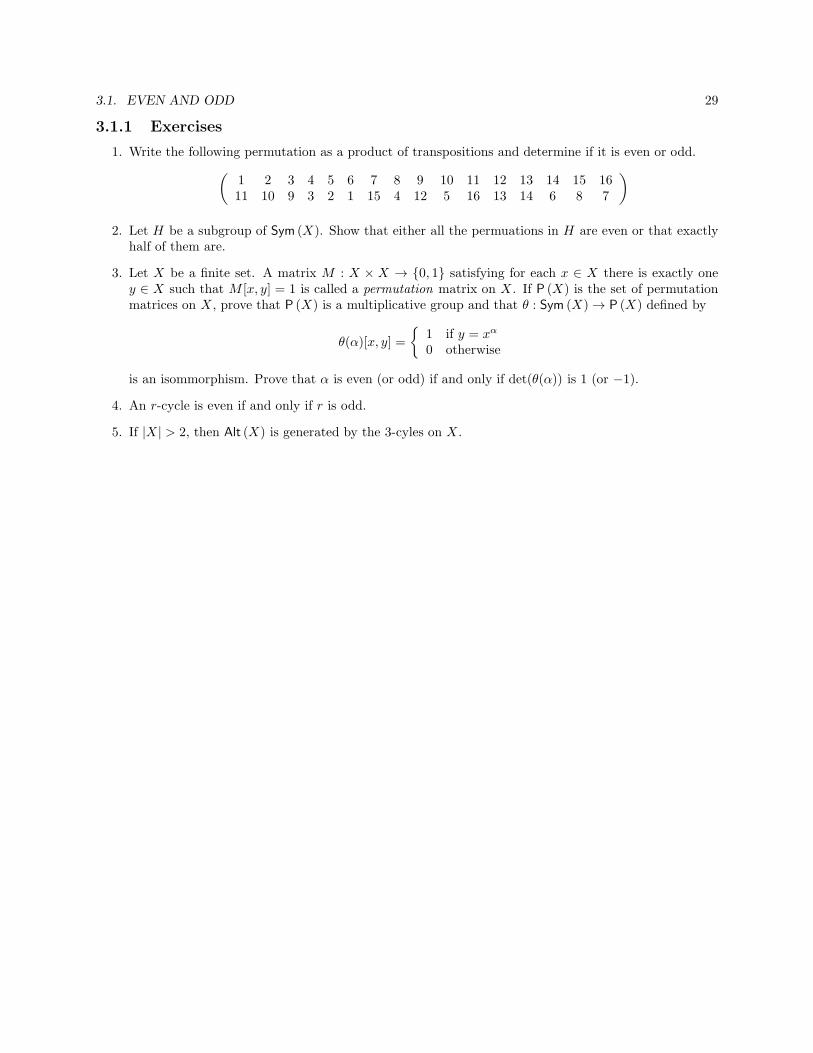
1. Write the following permutation as a product of transpositions and determine if it is even or odd.
(1 2 3 4 5 6 7 8 9 10 11 12 13 14 15 1611 10 9 3 2 1 15 4 12 5 16 13 14 6 8 7
)
2. Let H be a subgroup of Sym (X). Show that either all the permuations in H are even or that exactlyhalf of them are.
3. Let X be a finite set. A matrix M : X × X → 0, 1 satisfying for each x ∈ X there is exactly oney ∈ X such that M [x, y] = 1 is called a permutation matrix on X . If P (X) is the set of permutationmatrices on X , prove that P (X) is a multiplicative group and that θ : Sym (X)→ P (X) defined by
θ(α)[x, y] =
1 if y = xα
0 otherwise
is an isommorphism. Prove that α is even (or odd) if and only if det(θ(α)) is 1 (or −1).
4. An r-cycle is even if and only if r is odd.
5. If |X | > 2, then Alt (X) is generated by the 3-cyles on X .

30 CHAPTER 3. PERMUTATIONS
3.2 Group actions
Definition 3.3: A group G is said to act on the set Ω if there is a homomorphism g 7→ g of G intoSym (Ω).
Example 3.1: Some group actions.
1. Let S4 = Sym (1, 2, 3, 4). Then S4 acts on the set of ordered pairs:
Ω =
(X
2
)
= 1, 2, 1, 3, 1, 4, 2, 3, 2, 4, 3, 4 .
This action is given by i, jg = ig, jg . For example if g = (1, 2, 3)(4), then
g = (1, 2, 2, 3, 1, 3)(1, 4, 2, 4, 3, 4) .
2. We can extend the action of the group S4 to act on the subgraphs of K4, by applying the action aboveto each of the edges of the subgraph. For example if g = (1, 2, 3)(4), then
0
1 2
3 1
2 0
3 1
2 0
3
g g
g
Definition 3.4: Let G act on Ω. If x ∈ Ω and g ∈ G, the image of x under g is xg the application ofthe permutation g to x.
For example:
1
2 3
4 2
3 1
4
=
(1, 2, 3)(4)
Definition 3.5: Let G act on Ω.
• If x ∈ Ω, the orbit of x under G is
xG = xg : g ∈ Ga subset of Ω.
• If x ∈ Ω, the stabilizer of x under G is
Gx = g ∈ G : xg = xa subgroup of G.
(See Exercise 3.2.1.)
• The set of all orbits under the action of G on Ω is denoted by Ω/G.

3.2. GROUP ACTIONS 31
Example 3.2: Consider the action of S4 on Ω the 64 labeled subgraphs of K4 the complete subgraphon X = 1, 2, 3, 4.
• The orbit of1
2 3
4under G is
1
2 3
4,1
2 4
3,1
3 2
4,1
3 4
3,
1
4 2
3,1
4 3
2,2
1 3
4,2
1 4
3,
2
3 1
4,2
4 1
3,3
1 2
4,4
1 2
3
Observe that we may use the unlabeled picture to represent the orbit.
• The stabilizer of1
2 3
4under G is (1)(2)(3)(4) , (1, 4)(2, 3) .
• Ω/G =
, , , , , , , , , ,
Lemma 3.2.1 (Counting lemma) Let G act Ω. If x ∈ Ω, then |xG| = |G||Gx|
Proof. First note that Exercise 3.2.1 shows that Gx is a subgroup of G. Let x1, x2, ..., xm = xG. Then foreach i, 1 ≤ i ≤ m, there is a gi ∈ G such that xgi = xi. Suppose that Gxgi = Gxgj. Then gig
−1j ∈ Gx, and
hence xgig−1
j = x. Thus xi = xgi = xgjxj , and consequently xi = xj . Therefore the cosets Gxgi, 1 ≤ i ≤ m
are pairwise disjoint. Furthermore, if g ∈ G, then xg = xi for some i, 1 ≤ i ≤ m. Hence xgg−1
i = x. Thusgg−1
i ∈ Gx, and so g ∈ Gxgi. Consequently
G = Gxg1∪Gxg2∪Gxg3∪ · · · ∪Gxgm
Therefore by Lagrange’s Theorem (Theorem 2.2.3) m = |G : Gx| = |G||Gx|
If G acts on Ω, then the orbits under G partition the the objects in Ω. Counting the number of orbitsis very useful. For example the number of orbits of subgraphs under the action of S4 is the number ofnon-isomorphic subgraphs of S4. We will use Lemma 3.2.1 to establish the beautiful and useful theorem ofFrobenius, Cauchy and Burnside that counts the number of orbits. First observe that G acts on the subsetsof Ω in a natural way. Also, if g ∈ G, let χk(g) denote the number of k-element subsets fixed by g.
χk(g) = |S ⊆ Ω : |S| = k and Sg = S|
If S ⊆ Ω, then Sg = xg : x ∈ S.
Theorem 3.2.2 Let G be a group acting on the set Ω. Then the number of orbits of
(Ω
k
)
(the k–element
subsets of Ω) under G is∣∣∣∣
(Ω
k
)
/G
∣∣∣∣=
1
|G|∑
g∈G
χk(g)

32 CHAPTER 3. PERMUTATIONS
Proof. Let Nk =
∣∣∣∣
(Ω
k
)
/G
∣∣∣∣. Define an array whose rows are labeled by the elements of G and whose
columns are labeled by the k element subsets of Ω. The (g, S)–entry of the array is a 1 if Sg = S and is 0otherwise. Thus the sum of the entries of row g is precisely χk(g) and the sum of the entries in column S is|GS |. Hence ∑
g∈G
χk(g) =∑
S⊆Ω,|S|=k
|GS | (3.1)
Now partition the k-element subsets into the Nk orbits O1,O2, . . . ,ONkunder G. Choose a fixed repre-
sentative Si ∈ Oi for each i = 1, 2, . . . , Nk. Then for all S ∈ Oi, |GS | = |GSi| and the right hand side of
Equation 3.1 may be rewritten and Lemma 3.2.1 can be applied.
∑
g∈G
χk(g) =
Nk∑
i=1
|GSi| · |G(Si)|
=
Nk∑
i=1
|G| = Nk|G|
This establishes the result.
Example 3.3: Number of non-isomorphic graphs To count the number of graphs on 4 vertices Theo-rem 3.2.2 can be used as follows. Let G = Sym (1, 2, 3, 4) and label the edges of K4 as in Figure 3.1.
3
0 1
2
a
c
b
e
d
f
Figure 3.1: Edge labeling of K4
Each permutation can be mapped to a permutation of the edges. For example g = (1, 2, 3) 7→ (a, b, c)(d, e, f).Thus for instance χ2(g) = 0 and χ3(g) = 2. That is g fixes no subgraphs with 2 edges and 2 subgraphs with3 edges. We tabulate this information in Table 3.1 for all elements of G. The last row of Table 3.1 Gives Nk
the number of non-isomorphic subgraphs of K4 with k–edges, k = 0, 1, 2, . . . , 6.

3.2. GROUP ACTIONS 33
Table 3.1: Numbers of non isomorphic subgraphs in K4
g χ0 χ1 χ2 χ3 χ4 χ5 χ6
(0)(1)(2)(3) 7→ (a)(b)(c)(d)(e)(f) 1 6 15 20 15 6 1(0)(1)(2, 3) 7→ (a)(b, c)(d, e)(f) 1 2 3 4 3 2 1(0)(1, 2)(3) 7→ (a, b)(c)(d)(e, f) 1 2 3 4 3 2 1(0)(1, 2, 3) 7→ (a, b, c)(d, f, e) 1 0 0 2 0 0 1(0)(1, 3, 2) 7→ (a, c, b)(d, e, f) 1 0 0 2 0 0 1(0)(1, 3)(2) 7→ (a, c)(b)(d, f)(e) 1 2 3 4 3 2 1(0, 1)(2)(3) 7→ (a)(b, d)(c, e)(f) 1 2 3 4 3 2 1(0, 1)(2, 3) 7→ (a)(b, e)(c, d)(f) 1 2 3 4 3 2 1(0, 1, 2)(3) 7→ (a, d, b)(c, e, f) 1 0 0 2 0 0 1(0, 1, 2, 3) 7→ (a, d, f, c)(b, e) 1 0 1 0 1 0 1(0, 1, 3, 2) 7→ (a, e, f, b)(c, d) 1 0 1 0 1 0 1(0, 1, 3)(2) 7→ (a, e, c)(b, d, f) 1 0 0 2 0 0 1(0, 2, 1)(3) 7→ (a, b, d)(c, f, e) 1 0 0 2 0 0 1(0, 2, 3, 1) 7→ (a, b, f, e)(c, d) 1 0 1 0 1 0 1(0, 2)(1)(3) 7→ (a, d)(b)(c, f)(e) 1 2 3 4 3 2 1(0, 2, 3)(1) 7→ (a, d, e)(b, f, c) 1 0 0 2 0 0 1(0, 2)(1, 3) 7→ (a, f)(b)(c, d)(e) 1 2 3 4 3 2 1(0, 2, 1, 3) 7→ (a, f)(b, d, e, c) 1 0 1 0 1 0 1(0, 3, 2, 1) 7→ (a, c, f, d)(b, e) 1 0 1 0 1 0 1(0, 3, 1)(2) 7→ (a, c, e)(b, f, d) 1 0 0 2 0 0 1(0, 3, 2)(1) 7→ (a, e, d)(b, c, f) 1 0 0 2 0 0 1(0, 3)(1)(2) 7→ (a, e)(b, f)(c)(d) 1 2 3 4 3 2 1(0, 3, 1, 2) 7→ (a, f)(b, c, e, d) 1 0 1 0 1 0 1(0, 3)(1, 2) 7→ (a, f)(b, e)(c)(d) 1 2 3 4 3 2 1
Sum 24 24 48 72 48 24 24Sum/|G| 1 1 2 3 2 1 1

34 CHAPTER 3. PERMUTATIONS
Table 3.2: The number of black and white 10 beaded necklaces..
number(g) type(g) χ1(g) number(g) · χ1(g)The 10 rotations
1 110 210 1 · 210 = 10241 25 22 1 · 25 = 324 52 22 4 · 22 = 164 101 21 4 · 21 = 8
The 10 flips5 12 24 26 5 · 26 = 3205 25 25 5 · 25 = 160
Sum 1560Sum|D10|
78
In order to efficiently compute the number of orbits of k-subsets we define the type of a permutation gby1
type(g) =
n∏
j=1
jtj = 1t1 2t2 · · · ntn
where tj is the number of cycles of length j in the cycle decomposition of g. If S is a k–element subset fixedby g, then S is a union of cycles of G. Suppose S uses cj cycles of length j. Then cj ≤ tj ,
∑
j j · cj = k and
the number of such fixed subsets is∏
j
(tjcj
).
Example 3.4: Counting necklaces
In the adjacent figure is a necklace with 10 black orwhite beads. To compute the number of number of10 beaded necklaces using black and white beads, wefirst observe that the symmetry group is the dihedralgroup D10 and enumerate the elements of each cycletype, determine the number of necklaces fixed by eachand use Theorem 3.2.2 to compute N1 = 78. Thenumber of these necklaces. The computation is donein Table 3.2.
If the symmetry group is related to the symmetric group then a useful observation is given in the followingtheorem.
Theorem 3.2.3 Two elements in Sn are conjugate if and only if they have the same type.
Proof. Recall that every permutation can be written as the product of cycles. Thus because the conjugateof a product is a product of the conjugates
g−1(xy)g = (g−1xg)(g−1yg)
it suffices to show this for cycles, i.e. permutations of type 1n−k k1. In this proof it will be convenient toexplicitly display the fixed points of our k-cycles.
Let α = (x0, x1, x2, . . . , xk−1)(xk)(xk+1) · · · (xn−1) and β = (y0, y1, y2, . . . , yk−1)(yk)(xk+1) · · · (xn−1) be
two cycles of length k in Sn. Define g ∈ Sn by g : xi 7→ yi, for i = 0, 1, 2, . . . , n− 1. We now compute yg−1αg
There are two cases.1Note this is just formal notation and not an actual product.

3.2. GROUP ACTIONS 35
Case 1: y = yi ∈ y0, y1, y2, . . . , yk−1.
yg−1αg
i = xαgi = xgi+1 = yi+1 = yβi
where the subscripts are written modulo k.
Case 2: y /∈ y0, y1, y2, . . . , yk−1.yg
−1αg = yαg = yg = y = yβ
Hence g−1αg = β.Conversely suppose α = (x0, x1, x2, . . . , xk−1)(xk)(xk+1) · · · (xn−1) is a k-cycle in Sn and let g ∈ Sn. Let
γ = g−1αg. Let yi = xgi . Then for all i ∈ 0, 1, . . . , k − 1
yγi = yg−1αg
i = xαgi = xgi+1 = yi+1
(subscripts modulo k).
If y /∈ y0, y1, y2, . . . , yk−1, then yg−1
/∈ x0, x1, x2, . . . , xk−1. So for such y
yγ = yg−1αg = (yg
−1
)αg = (yg−1
)g = y
Therefore γ is the k-cycle (y0, y1, . . . , yk−1)(yk)(xk+1) · · · (xn−1). Hence every conjugate of a k-cycle is ak-cycle.
Example 3.5: Quick conjugation in Sn To find an element g ∈ S12 to conjugate
α = (1, 2, 3, 4)(5, 6, 7, 8)(9, 10)(11)(12)
ontoβ = (5)(3, 1, 2, 6)(10, 4, 7, 11)(9, 8)(12).
We first arrange, anyway we like, the cycles of β under the cycles of α so that k-cycles are under k-cyclesk = 1, 2, 3, . . . , n. Remember there are k different ways to write the same k-cycle.
α = ( 1 , 2 , 3 , 4 )( 5 , 6 , 7 , 8 )( 9 , 10 )( 11 )( 12 )β = ( 4 , 7 , 11 , 10 )( 2 , 6 , 3 , 1 )( 9 , 8 )( 12 )( 5 )
Now define g ∈ S12 by g : x 7→ y if x in α appears directly above y in β. In our example we get
g =
(1 2 3 4 5 6 7 8 9 10 11 124 7 11 10 2 6 3 1 9 8 12 5
)
= (1, 4, 10, 8)(2, 7, 3, 11, 12, 5)(6)(9)
Then g−1αg = β. Indeed g is precisely the permutation defined in Theorem 3.2.3.
The computation in Example 3.5 also tells us how to compute the centralizer CSn(α) of α in Sn. For
after all g ∈ CSn(α) if and only if g conjugates α onto itself. Thus we let α play also the role of β in the
above computation.
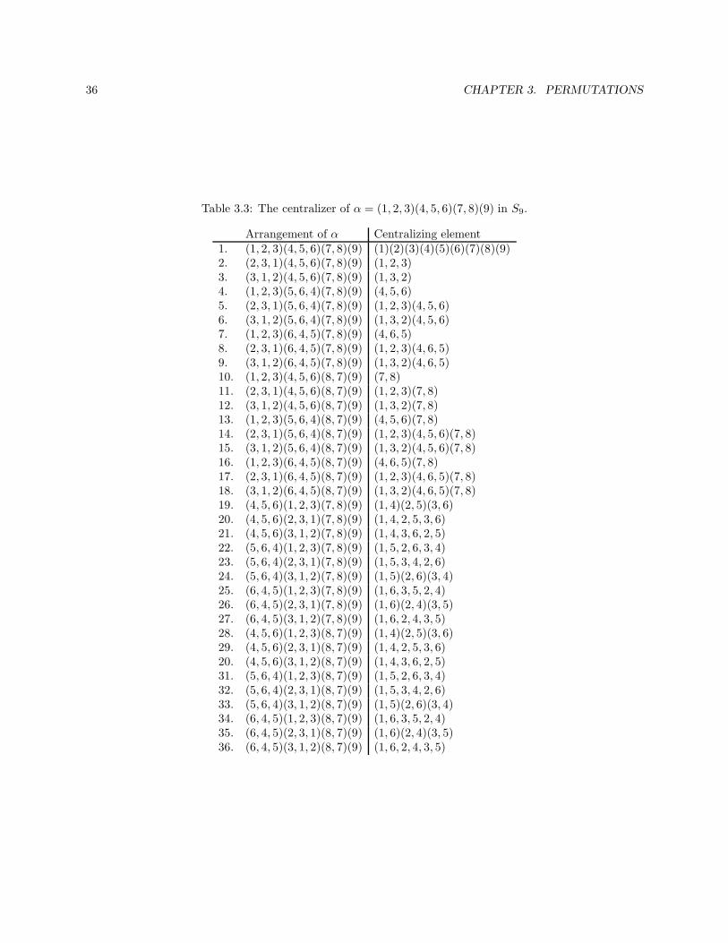
Example 3.6: Computing the centralizer in Sn To compute the centralizer of
α = (1, 2, 3)(4, 5, 6)(7, 8)(9).
in S9 we use the technique shown in Example 3.2. 3.5. Thus we arrange α under itself in all possible waysand write down the mapping g from one arrangement to the other. The set of all these gs is the centralizerCSn
(α). The computations are done in Table 3.3 The centralizer of α are the 36 permutations that appearin the last column of the table.
Notice that the number of permutations in Sn that centralize a permutation α ∈ Sn is just the number ofways to arrange the cycles of α under itself so that k-cycles are below k-cycles. If α has tj j-cycles, there arejtj tj ! ways to arrange them, since each can be put in anyone of tj positions and each j-cycle has j equivalentdescriptions. Thus we have the following theorem.
36 CHAPTER 3. PERMUTATIONS
Table 3.3: The centralizer of α = (1, 2, 3)(4, 5, 6)(7, 8)(9) in S9.
Arrangement of α Centralizing element1. (1, 2, 3)(4, 5, 6)(7, 8)(9) (1)(2)(3)(4)(5)(6)(7)(8)(9)2. (2, 3, 1)(4, 5, 6)(7, 8)(9) (1, 2, 3)3. (3, 1, 2)(4, 5, 6)(7, 8)(9) (1, 3, 2)4. (1, 2, 3)(5, 6, 4)(7, 8)(9) (4, 5, 6)5. (2, 3, 1)(5, 6, 4)(7, 8)(9) (1, 2, 3)(4, 5, 6)6. (3, 1, 2)(5, 6, 4)(7, 8)(9) (1, 3, 2)(4, 5, 6)7. (1, 2, 3)(6, 4, 5)(7, 8)(9) (4, 6, 5)8. (2, 3, 1)(6, 4, 5)(7, 8)(9) (1, 2, 3)(4, 6, 5)9. (3, 1, 2)(6, 4, 5)(7, 8)(9) (1, 3, 2)(4, 6, 5)10. (1, 2, 3)(4, 5, 6)(8, 7)(9) (7, 8)11. (2, 3, 1)(4, 5, 6)(8, 7)(9) (1, 2, 3)(7, 8)12. (3, 1, 2)(4, 5, 6)(8, 7)(9) (1, 3, 2)(7, 8)13. (1, 2, 3)(5, 6, 4)(8, 7)(9) (4, 5, 6)(7, 8)14. (2, 3, 1)(5, 6, 4)(8, 7)(9) (1, 2, 3)(4, 5, 6)(7, 8)15. (3, 1, 2)(5, 6, 4)(8, 7)(9) (1, 3, 2)(4, 5, 6)(7, 8)16. (1, 2, 3)(6, 4, 5)(8, 7)(9) (4, 6, 5)(7, 8)17. (2, 3, 1)(6, 4, 5)(8, 7)(9) (1, 2, 3)(4, 6, 5)(7, 8)18. (3, 1, 2)(6, 4, 5)(8, 7)(9) (1, 3, 2)(4, 6, 5)(7, 8)19. (4, 5, 6)(1, 2, 3)(7, 8)(9) (1, 4)(2, 5)(3, 6)20. (4, 5, 6)(2, 3, 1)(7, 8)(9) (1, 4, 2, 5, 3, 6)21. (4, 5, 6)(3, 1, 2)(7, 8)(9) (1, 4, 3, 6, 2, 5)22. (5, 6, 4)(1, 2, 3)(7, 8)(9) (1, 5, 2, 6, 3, 4)23. (5, 6, 4)(2, 3, 1)(7, 8)(9) (1, 5, 3, 4, 2, 6)24. (5, 6, 4)(3, 1, 2)(7, 8)(9) (1, 5)(2, 6)(3, 4)25. (6, 4, 5)(1, 2, 3)(7, 8)(9) (1, 6, 3, 5, 2, 4)26. (6, 4, 5)(2, 3, 1)(7, 8)(9) (1, 6)(2, 4)(3, 5)27. (6, 4, 5)(3, 1, 2)(7, 8)(9) (1, 6, 2, 4, 3, 5)28. (4, 5, 6)(1, 2, 3)(8, 7)(9) (1, 4)(2, 5)(3, 6)29. (4, 5, 6)(2, 3, 1)(8, 7)(9) (1, 4, 2, 5, 3, 6)20. (4, 5, 6)(3, 1, 2)(8, 7)(9) (1, 4, 3, 6, 2, 5)31. (5, 6, 4)(1, 2, 3)(8, 7)(9) (1, 5, 2, 6, 3, 4)32. (5, 6, 4)(2, 3, 1)(8, 7)(9) (1, 5, 3, 4, 2, 6)33. (5, 6, 4)(3, 1, 2)(8, 7)(9) (1, 5)(2, 6)(3, 4)34. (6, 4, 5)(1, 2, 3)(8, 7)(9) (1, 6, 3, 5, 2, 4)35. (6, 4, 5)(2, 3, 1)(8, 7)(9) (1, 6)(2, 4)(3, 5)36. (6, 4, 5)(3, 1, 2)(8, 7)(9) (1, 6, 2, 4, 3, 5)

3.2. GROUP ACTIONS 37
Table 3.4: Numbers of non isomorphic subgraphs in K4
type(g)|K(g)|vert.edges|K(g)|χ0|K(g)|χ1|K(g)|χ2|K(g)|χ3|K(g)|χ4|K(g)|χ5|K(g)|χ6
1 14 16 1 · 1 1 · 2 1 · 3 1 · 4 1 · 3 1 · 2 1 · 16 12 21 12 22 6 · 1 6 · 2 6 · 3 6 · 4 6 · 3 6 · 2 6 · 18 11 31 32 8 · 1 8 · 0 8 · 0 8 · 2 8 · 0 8 · 0 8 · 13 22 12 22 3 · 1 3 · 2 3 · 3 3 · 4 3 · 3 3 · 2 3 · 16 41 21 41 6 · 1 6 · 0 6 · 1 6 · 0 6 · 1 6 · 0 6 · 1
Sum 24 24 48 72 48 24 24Sum|G| 1 1 2 3 2 1 1
Theorem 3.2.4 If g ∈ Sn has type(g) = 1t1 2t2 · · · ntn, then the order2 of the centralizer of g is |CSn
(g)| =n∏
k=1
jtj tj !.
Putting this all together we obtain the following very useful corollary.
Corollary 3.2.5 The number of element of type 1t1 2t2 · · · ntn in Sn is n!/∏n
k=1 jtj tj !.
Proof. If g ∈ Sn has type(g) = 1t1 2t2 · · · ntn , then by Theorem 3.2.3 all elements of this type areconjugate to g. The number of these is thus the size |KSn
(g)| of the conjugacy class of g. By Theorem 2.7.1we have |KSn
(g)| = (n!)/|CSn(g)|. Now apply Theorem 3.2.4 to obtain the desired result.
Using this concept of type the computations in Table 3.1 can be simplified. The new calculations arepresented in simple Table 3.1.
We close this section with an application of Corollary 3.2.5. There is important discussion in the proofof the following theorem and the reader is encouraged to study it.
Theorem 3.2.6 The alternating group A4 is a group of order 12 with no subgroup of order 6.
Proof. If H is a subgroup of order 6 in A4, then the |A4 : H | = 2, and thus H is normal in A4. Consequently,H is a union of conjugacy classes in A4.
The group A4 is the set of even permutations in S4 and these have type 14, 22, and 11 31. respectively.Applying Corollary 3.2.5 we see that there are 1, 3, and 8 permutations of these types respectively. Althoughthis accounts for the 12 elements of A4 this does not give us the size of the conjugacy classes in A4. Elementsthat are conjugate in S4 need not be conjugate in A4.
For example if g = (1)(2, 3, 4), (so g has type 11 31), then using the techniques of Example 3.6 we seethat
CS4(g) = (1)(2)(3)(4), (1)(2, 3, 4), (1)(2, 4, 3).
Each of these are even permutations and so CS4(g) = CA4
(g). Hence |CA4(g)| = 3 and therefore g has
|A4|/|CA4(g)| = 12/3 = 4 conjugates. Thus 4 of the 8 elements of type 11 31 are conjugate in A4.
Consequently there are 2 classes of elements of type 11 31, making two classes of size 4.If on the other hand g has type 22, say g = (1, 2)(3, 4), then
CS4(g) =
(1)(2)(3)(4), (1, 2)(3, 4), (1, 3)(2, 4),(1, 4)(2, 3), (1, 2), (3, 4), (1, 3, 2, 4), (1, 4, 2, 3)
,
2This is not formal notation but the actual product of the numbers involved in the notation for the type.

38 CHAPTER 3. PERMUTATIONS
and soCA4
(g) = (1)(2)(3)(4), (1, 2)(3, 4), (1, 3)(2, 4), (1, 4)(2, 3).Thus the number of conjugates of g in A4 is 12
4 = 3, which accounts for all of the type 22 elements. So, A4
has a conjugacy class of size 3.Lastly, there is the type 14 class which only contains the identity. A class of size 1.We see now that A4 has 4 conjugacy classes and they have sizes 1, 3, 4, and 4. If A4 has a subgroup of
order 6 it would be normal and thus a union of conjugacy classes. So 6 would have to be able to be writtenas sum from the numbers 1, 3, 4 and 4 and this is impossible. Therefore A4 has no subgroup of order 6.
3.2.1 Exercises
1. Let G act on Ω and suppose that x ∈ Ω. Show that the stabilizer Gx is a subgroup of G.
2. Consider the permutations
α = (1, 2, 3)(4, 5, 6, 7, 8)
β = (1, 3, 2)(4, 8, 7, 6, 5)
(a) In S8 is α conjugate to β?
(b) In A8 is α conjugate to β?
(c) What is the centralizer of α in S8?
(d) What is the centralizer of β in S8?
(e) What is the centralizer of α in A8?
(f) What is the centralizer of β in A8?
(g) How many conjugates in S7 does α have? What about β?
(h) How many conjugates in A7 does α have? What about β?
3. A group G is said to be simple if and only if G has no proper normal subgroup.
(a) Find the sizes of the conjugacy classes of A5 the set of even permutations on 1, 2, 3, 4, 5.(b) Show that A5 is a simple group.
(c) Let G be a finite group of order |G| = n and let H ≤ G be a proper subgroup of index |G : H | = r.Show that if n > r!, then G has a proper normal subgroup and hence cannot be simple. (Hint:Let G act on the right cosets of H by right mutiplication.)
4. (a)How many distinct n by n tablecloths can be made if thereare q colors available to color the n2 boxes.
×
⋆
t
⋆×
×
⋆×
t
×
t
⋆
t
t
×
t
t
⋆
t
⋆×
⋆⋆⋆
×
⋆⋆⋆
t
×
t
⋆
t
⋆⋆×
(b) If there are q colors available how many colored roulette wheels are there with n compartments.

3.3. THE SYLOW THEOREMS 39
3.3 The Sylow theorems
Definition 3.6: A finite group G is a p-group if |G| = px, for some prime p and positive integer x. Amaximal p-subgroup of a finite group G is called a Sylow-p subgroup of G.
If P is a Sylow-p subgroup of G and H is a p-subgroup of G such that P ⊆ H , then H = P .
Definition 3.7: Let H be a subgroup of a group G. A subgroup S of G is conjugate to H if and onlyif S = g−1Hg for some g ∈ G.
Notice that conjugate subgroups are isomorphic.
Definition 3.8: Let H be a subgroup of G. The normalizer of H in G is
NG(H) = g ∈ G : g−1Hg = H
The normalizer NG(H) of H in G is the largest subgroup of G in which H is normal. We establish twotechnical lemmas.
Lemma 3.3.1 Let P be a Sylow-p subgroup of G. Then NG(P )/P has no element whose order is a powerof p except for the identity.
Proof. Suppose g ∈ NG(P )/P has order a power of p. Let S = 〈g〉 a subgroup of NG(P )/P . Then there isa subgroup S of G containing P such that S = S/P , (See Theorem ??.) Because S and P are both p-groups,it follows that S is a p-group. But the maximality of P implies P = S. Therefore S = 1 and g = 1.
Lemma 3.3.2 Let P be Sylow-p subgroup of G and let g ∈ G have order a power of p. If g−1Pg = P , theng ∈ P .
Proof. Because g ∈ NG(P ), then gP ∈ NG(P )/P . Furthermore g has order a power of p, so therefore gPhas order a power of p But by Lemma 3.3.1 gP is P the identity of NG(P )/P . Consequently g ∈ P .
A finite group G acts on its subgroups via conjugation. If H is a subgroup of G, then the stabilizerof H under this action is GH = NG(H) and the orbit of H is the set of conjugates of H . The number ofconjugates is thus |G : NG(H)|. (See Theorem 2.7.1.) We pursue this idea of acting on the subgroups of Gin the next theorem. Keep in mind that the conjugate of a Sylow-p subgroup is a Sylow-p subgroup. Let Np
be the number of Sylow-p subgroups of G.
Theorem 3.3.3 (Sylow) Let G be a finite group with Sylow-p subgroup P .
1. All Sylow-p subgroups of G are conjugate to P .
2. Np ≡ 1 mod p and Np |G|.

40 CHAPTER 3. PERMUTATIONS
Proof.Let Ω be the set of conjugates of P : say
Ω = P1, P2, P3, . . . , Pr
where P = P1. Then G acts on Ω via conjugation. In fact any subgroup of G acts on Ω. In particular P actson Ω. Lemma 3.3.2 shows that the stabilizer of P1 under the action of P is PP1
= P , because P = P1. Thusin this action P1 is an orbit of length 1. Lemma 3.3.2 also says |PPj
| 6= 1 if j 6= 1. Thus the remaining Pj
are in orbits whose lengths are a power of p greater than 1. Therefore |Ω| ≡ 1 mod p.Now if Q is any sylow p-subgroup that is not conjugate to P , then Q also acts on Ω. The same argument
as above will show that the orbits under this action of Q will all have length a power of p greater than 1.This would imply that p |Ω| contrary to the above. Thus all Sylow-p subgroups of G are conjugate to P and
Np = |Ω|. So Np ≡ 1 mod p and Np |G|, for after all |Ω| is an orbit under G and so |Ω| divides |G|.
Theorem 3.3.4 (Sylow) Let G be a finite group of order |G| = pxm, where p 6 m, then every Sylow-p
subgroup of G has order pk.
Proof. Observe that |G : P | = |G : NG(P )||NG(P ) : P |. Now |G : NG(P )| = Np ≡ 1 mod p, sop 6 |G : NG(P )|. Also |NG(P ) : P | = |NG(P )/P |. Using Lemma 3.3.1 we see that NG(P )/P has
no elements order p. Thus by Cauchy’s Theorem (Theorem 2.7.4) we see that p 6 |NG(P )/P |. Hence
p 6 |G : P |. Therefore m = |G : P | and so |P | = px.
3.3.1 Exercises
1.m A group G is said to be simple if and only if G has no proper normal subgroup.
(a) Let G be a finite group of order |G| = n and let H ≤ G be a proper subgroup of index |G : H | = r.Show that if n > r!, then G has a proper normal subgroup (contained in H) and hence cannot besimple.
(b) Show that every non–abelian group of order less than 60 has a normal subgroup and is thereforenot simple.
(c) Use the above and Exercise 3.2.1 3b to conclude that A5 is the smallest non–abelian simple group.(You don’t need to show this but the next smallest non–abelain simple group has 168 elements.)

3.4. SOME APPLICATIONS OF THE SYLOW THEOREMS 41
3.4 Some applications of the Sylow Theorems
Definition 3.9: Let H and K be groups the direct product of H and K is the group H ×K
H ×K = (h, k) : h ∈ H and k ∈ K
with multiplication (h1, k1)(h2, k2) = (h1h2, k1k2).
Theorem 3.4.1 Let H and K be subgroups of the group G. If
(1) G = HK,
(2) H and K are both normal subgroups of G, and
(3) H ∩K = 1,
then G ∼= H ×K
Proof. First of all we have from (1) that every element g ∈ G can be written as a product g = hk whereh ∈ H and k ∈ K. Property (3) shows that the choice of h and k is unique, for if h1k1 = h2k2, thenh−12 h1 = k2k
−11 ∈ H ∩K. And so h1 = h2 and k1 = k2. This says that the map θ : G → H ×K given by
hk 7→ (h, k) is well defined. It is obviously onto. To see that it is a homomorphism first consider arbitraryelements h ∈ H and k ∈ K. Then
h−1k−1hk = h−1(k−1hk) ∈ H because H is normal
h−1k−1hk = (h−1k−1h)k ∈ K because K is normal
Thus by (3) h−1k−1hk = 1 and so hk = kh for all h ∈ H , k ∈ K. Now let g1 = h1k1 g2 = h2k2 be elementsof G, h1, h2 ∈ H and k1, k2 ∈ K. Then
θ(g1g2) = θ(h1k1h2k2) = θ(h1h2k1k2)
= (h1h2, k1k2) = (h1, k1)(h2, k2)
Therefore θ is a homomorphism. Furthermore g = hk ∈ kernel (θ) if and only if θ(hk) = (h, k) = (1, 1). Thuskernel (θ) = 1, and therefore θ : G→ H ×K is an isomorphism.
Corollary 3.4.2 If gcd (m,n) = 1, then Zmn∼= Zm × Zn.
Proof. We know by Theorem 2.3.3 that Zmn has a subgroup H ∼= Zm and a subgroup K ∼= Zn. Theseare normal subgroups because Zmn is abelian. Furthermore, gcd (m,n) = 1 so H ∩ K = 1. ThereforeTheorem 3.4.1 gives the result.
Definition 3.10: The dihedral group Dn, n ≥ 2 is a group of order 2n generated by two elements aand b satisfying the relations
an = 1, b2 = 1, and bab = a−1
The relations for the dihedral group show that ba = a−1b and hence any product written in the generatorsa and b is equal to a product of the form aibj where 0 ≤ i < n and 0 ≤ j < 2. Thus Dn will have 2n elements

42 CHAPTER 3. PERMUTATIONS
should it exist. But of course it exists. It is the symmetry group of an n-gon is a dihedral group Dn. In factwe may take a and b to be the functions on Zn defined by
a : x 7→ x+ 1 (modn) and b : x 7→ −x (modn) and b : x 7→ −x (modn)
Then an(x) = b2(x) = x for all x ∈ Zn. Hence an and b2 are the identity function. Also,
(bab)(x) = (ba)(b(x)) = (ba)(−x) = b(a(−x)) = b(−x+ 1) = (x − 1)a−1(x).
Theorem 3.4.3 Every group of order 2p is either cyclic or dihedral.
Proof. Let G be a group of order 2p. Then by Cauchy’s Theorem (Theorem 2.7.4), G contains an elementa of order p and an element b of order 2. Let H = 〈a〉, then |G : H | = 2 and so H is normal in G. Thereforebab = ai for some i, because b−1 = b. Now
a = b2ab2 = b(bab)b = b(ai)b = (bab)i = (ai)i = ai2
Thus ai2−1 = 1, and so p (i2 − 1). Consequently, p (i− 1) or p (i + 1).
If p (i − 1), then ai−1 = 1, so ai = a, hence bab = a. Therefore G is abelian. So 〈b〉 is normal in G andtherefore applying Theorem 3.4.1 we have that G is isomorphic to the direct product 〈a〉×〈b〉 ∼= Zp×Z2
∼= Z2p,because gcd (2, p) = 1. Therefore G is cyclic.
If p (i+ 1), then ai+1 = 1, so ai = a−1, hence bab = a−1. Therefore G is dihedral.
Theorem 3.4.4 If G is a group of order |G| = pq, where p > q are primes. If q does not divide p− 1, thenG is cyclic.
Proof. Let Np be the number of Sylow-p subgroups, then Np ≡ 1 mod p and Np divides q. Hence Np = 1because p > q. Therefore the Sylow-p subgroup H is normal in G.
Let Nq be the number of Sylow-q subgroups, then Nq ≡ 1 mod q and Nq divides p. Hence Nq = 1 or pbecause p is a prime. If Np = p, we have p ≡ 1 mod q and so q divides p − 1 contrary to the hypothesis.Therefore Nq = 1 and the Sylow-q subgroup K is normal in G.
Obviously H ∩K = 1 so Theorem 3.4.1 applies and we see that
G ∼= H ×K ∼= Zp × Zq∼= Zpq.
Consequently, G is cyclic as claimed.
Theorem 3.4.5 If G is a group of order |G| = pq, where p > q are primes. If q divides p− 1, then eitherG is cyclic or G is generated by two elements a and b satisfying
ap = 1, bq = 1, and b−1ab = ar,
where r 6≡ 1 (mod p), but rq ≡ 1 (mod p).
Proof. By Cauchy’s Theorem (Theorem 2.7.4) there exists an elements a, b ∈ G of order p and q respectively.The proof of Theorem 3.4.4 shows that 〈a〉 E G and if 〈b〉 E G, then G is cyclic. Furthermore if q 6 p − 1,
then necessarily 〈b〉 E G. So we suppose q (p − 1) and 〈b〉 is not a normal a subgroup. In particular G isnot abelian. Then because 〈a〉 E G, we have
bab−1 = ar

3.4. SOME APPLICATIONS OF THE SYLOW THEOREMS 43
for some r. Hence r 6≡ 1 (mod p), because G is not abelian. Furthermore for all j
bjab−j = bj−1(bab−1)b−(j−1) = bj−1arb−(j−1
= bj−2(barb−1)b−(j−2) = bj−2ar2
b−(j−2)
= bj−3(bar2
b−1)b−(j−3) = bj−3ar3
b−(j−3)
...
= arj
In particular if j = q, we obtain a = arq
and therefore rq ≡ 1 (mod p).
Definition 3.11: The quaterians Q, is a group of order 8 generated by two elements a and b satisfyingthe relations
a4 = 1, b2 = a2, and b−1ab = a−1
The relations for the Quaterians group show that ba = a−1b and hence any product written in thegenerators a and b is equal to a product of the form aibj where 0 ≤ i < n and 0 ≤ j < 2. Thus Q will have8 elements should it exist. The permutations
a = (1, 2, 3, 4)(5, 6, 7, 8)
b = (1, 5, 3, 7)(2, 6, 4, 8)
can be easily shown to satisfy the Quaterian relations.
Theorem 3.4.6 The only non–abelian groups of order 8 are Q and D4.
Proof. Let G be a non–abelian group of order 8. Then G contains no element of order 8, for then it wouldbe cyclic and by Exercise 1.2.1.5a G must have an element a of order 4. Then 〈a〉 has index 2 in G and istherefore normal and thus G/ 〈a〉 ∼= Z2 Thus by Lagrange (Theorem 2.2.3) G = 〈a〉 ∪ 〈a〉 b for some b ∈ G,b /∈ 〈a〉 and so b2 ∈ 〈a〉 = 1, a, a2, a3. Consequently
b2 = 1 or b2 = a2
for if b2 = a or b2 = a3, then b would have order 8 which is a contradiction. Furthermore, because 〈a〉 is anormal subgroup, b−1ab ∈ 〈a〉 and thus
b−1ab = a or b−1ab = a3.
We can only have the later possibility, because G is non–abelian. Therefore either
(1) a4 = 1, b2 = 1, and b−1ab = a3
or
(2) a4 = 1, b2 = a2, and b−1ab = a3
Because a3 = a−1, (1) describes D4 and (2) describes Q.
Theorem 3.4.7 Every group G of order 12 that is not isomorphic to A4 contains an element of order 6and a normal Sylow-3 subgroup.
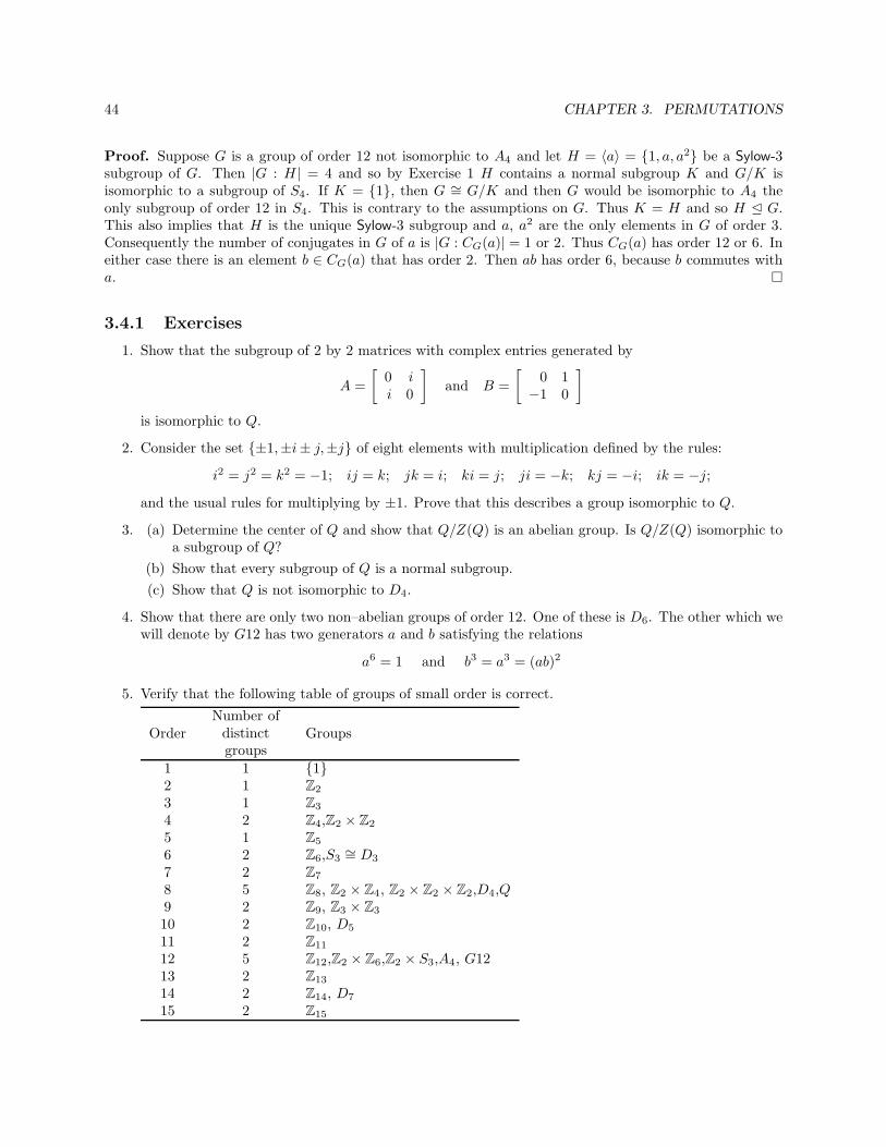
44 CHAPTER 3. PERMUTATIONS
Proof. Suppose G is a group of order 12 not isomorphic to A4 and let H = 〈a〉 = 1, a, a2 be a Sylow-3subgroup of G. Then |G : H | = 4 and so by Exercise 1 H contains a normal subgroup K and G/K isisomorphic to a subgroup of S4. If K = 1, then G ∼= G/K and then G would be isomorphic to A4 theonly subgroup of order 12 in S4. This is contrary to the assumptions on G. Thus K = H and so H E G.This also implies that H is the unique Sylow-3 subgroup and a, a2 are the only elements in G of order 3.Consequently the number of conjugates in G of a is |G : CG(a)| = 1 or 2. Thus CG(a) has order 12 or 6. Ineither case there is an element b ∈ CG(a) that has order 2. Then ab has order 6, because b commutes witha.
3.4.1 Exercises
1. Show that the subgroup of 2 by 2 matrices with complex entries generated by
A =
[0 ii 0
]
and B =
[0 1−1 0
]
is isomorphic to Q.
2. Consider the set ±1,±i± j,±j of eight elements with multiplication defined by the rules:
i2 = j2 = k2 = −1; ij = k; jk = i; ki = j; ji = −k; kj = −i; ik = −j;and the usual rules for multiplying by ±1. Prove that this describes a group isomorphic to Q.
3. (a) Determine the center of Q and show that Q/Z(Q) is an abelian group. Is Q/Z(Q) isomorphic toa subgroup of Q?
(b) Show that every subgroup of Q is a normal subgroup.
(c) Show that Q is not isomorphic to D4.
4. Show that there are only two non–abelian groups of order 12. One of these is D6. The other which wewill denote by G12 has two generators a and b satisfying the relations
a6 = 1 and b3 = a3 = (ab)2
5. Verify that the following table of groups of small order is correct.
OrderNumber ofdistinctgroups
Groups
1 1 12 1 Z2
3 1 Z3
4 2 Z4,Z2 × Z2
5 1 Z5
6 2 Z6,S3∼= D3
7 2 Z7
8 5 Z8, Z2 × Z4, Z2 × Z2 × Z2,D4,Q9 2 Z9, Z3 × Z3
10 2 Z10, D5
11 2 Z11
12 5 Z12,Z2 × Z6,Z2 × S3,A4, G1213 2 Z13
14 2 Z14, D7
15 2 Z15

Chapter 4
Finitely generated abelian groups
4.1 The Basis Theorem
The usual custom for abelian groups is to adopt additive notation instead of multiplicative. The followingtable provides the translation:
Multiplication ←→ Additionab ←→ a+ b1 ←→ 0
a−1 ←→ −aan ←→ na
ab−1 ←→ a− baH ←→ a+H
direct product ←→ direct sumH ×K ←→ H ⊕K
m∏
i=1
Hi ←→m∑
i=1
Hi
Let A be an abelian group.
1. If a, b ∈ A and n ∈ Z, then n(a+ b) = na+ nb.
2. If A = 〈a1, a2, . . . , ak〉, then A = n1a1 + n2a2 + · · · + nnak : n1, n2, . . . , nk ∈ Z the set of all linearcombinations of the elements a1, a2, . . . , ak with integer coefficients.
In particular Theorem 3.4.1 becomes
Theorem 4.1.1 Let H and K be subgroups of the abelian group A. If
1. G = H +K,
2. H ∩K = 1,
then A ∼= H ⊕K
and the second isomorphism law is;
Theorem 4.1.2 (Second law) Let H and N be subgroups of the abelian group A. Then H/(H ∩ N) ∼=(N +H)/N .
45
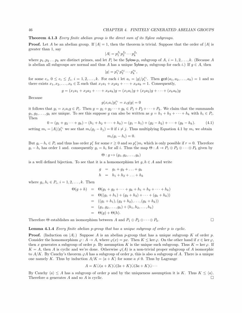
46 CHAPTER 4. FINITELY GENERATED ABELIAN GROUPS
Theorem 4.1.3 Every finite abelian group is the direct sum of its Sylow subgroups.
Proof. Let A be an abelian group. If |A| = 1, then the theorem is trivial. Suppose that the order of |A| isgreater than 1, say
|A| = pf11 pf22 · · · pfkk
where p1, p2 . . . pk are distinct primes, and let Pi be the Sylow-pi subgroup of A, i = 1, 2, . . . , k. (Because Ais abelian all subgroups are normal and thus A has a unique Sylow-pi subgroup for each i.) If g ∈ A, then
|g| = pe11 pe22 · · · pekk ,
for some ei, 0 ≤ ei ≤ fi, i = 1, 2, . . . , k. For each i let ai = |g|/peii . Then gcd (a1, a2, . . . , ak) = 1 and sothere exists x1, x2, . . . , xk ∈ Z such that x1a1 + x2a2 + · · ·+ xkak = 1. Consequently,
g = (x1a1 + x2a2 + · · ·+ xkak)g = (x1a1)g + (x2a2)g + · · ·+ (xkak)g
Becauseg(xiai)p
eii = xig|g| = 0
it follows that gi = xiaig ∈ Pi. Then g = g1+ g2 · · ·+ gk ∈ P1 +P2 + · · ·+Pk. We claim that the summandsg1, g2, . . . , gk are unique. To see this suppose g can also be written as g = h1 + h2 + · · ·+ hk with hi ∈ Pi.Then
0 = (g1 + g2 · · ·+ gk)− (h1 + h2 + · · ·+ hk) = (g1 − h1) + (g2 − h2) + · · ·+ (gk − hk). (4.1)
setting mi = |A|/peii we see that mi(gj − hj) = 0 if i 6= j. Thus multiplying Equation 4.1 by mi we obtain
mi(gi − hi) = 0.
But gi−hi ∈ Pi and thus has order pri for some r ≥ 0 and so pri |mi which is only possible if r = 0. Thereforegi − hi has order 1 and. consequently gi = hi for all i. Thus the map Θ : A→ P1 ⊕ P2 ⊕ · · · ⊕ Pk given by
Θ : g 7→ (g1, g2, . . . , gk)
is a well defined bijection. To see that it is a homomorphism let g, h ∈ A and write
g = g1 + g2 + . . .+ gk
h = h1 + h2 + . . .+ hk
where gi, hi ∈ Pi, i = 1, 2, . . . , k. Then
Θ(g + h) = Θ(g1 + g2 + · · ·+ gk + h1 + h2 + · · ·+ hk)
= Θ((g1 + h1) + (g2 + h2) + · · ·+ (gk + hk))
= ((g1 + h1), (g2 + h2), . . . , (gk + hk))
= (g1, g2, . . . , gk) + (h1, h2, . . . , hk)
= Θ(g) + Θ(h).
Therefore Θ establishes an isomorphism between A and P1 ⊕ P2 ⊕ · · · ⊕ Pk.
Lemma 4.1.4 Every finite abelian p-group that has a unique subgroup of order p is cyclic.
Proof. (Induction on |A|.) Suppose A is an abelian p-group that has a unique subgroup K of order p.Consider the homomorphism ϕ : A→ A, where ϕ(x) = px. Then K ≤ kerϕ. On the other hand if x ∈ kerϕ,then x generates a subgroup of order p. By assumption K is the unique such subgroup. Thus K = kerϕ. IfK = A, then A is cyclic and we’re done. Otherwise ϕ(A) is a non-trivial proper subgroup of A isomorphicto A/K. By Cauchy’s theorem ϕA has a subgroup of order p, this is also a subgroup of A. There is a uniqueone namely K. Thus by induction A/K = 〈a+K〉 for some a 6= 0. Thus by Lagrange
A = K∪(a+K)∪(2a+K)∪(3a+K)∪ · · ·By Cauchy 〈a〉 ≤ A has a subgroup of order p and by the uniqueness assumption it is K. Thus K ≤ 〈a〉.Therefore a generates A and so A is cyclic.

4.1. THE BASIS THEOREM 47
Lemma 4.1.5 If A is a finite abelian p-group and C ≤ A is cyclic subgroup of maximal order, then A =C ⊕H, for some subgroup H.
Proof. (Induction on |A|.) If A is cyclic we’re done, so suppose A is not cyclic. Then by Lemma 4.1.4 Ahas at least two cyclic subgroups of order p while C can have only one. Hence there exist a cyclic subgroupK ≤ A of order p, that is not contained in C. Consequently by Theorem 2.6.3 (Second law)
(C +K)/K ∼= C/(C ∩K) = C
Given any g ∈ A, by the Law of correspondence (Theorem 2.6.5) the order of g+K in A/K divides |g| whichis at most |C|, because C is a cyclic subgroup of maximal order. Thus the subgroup (C +K)/K is a cyclicsubgroup of maximal order in A/K and we can apply the inductive hypothesis to obtain
A/K = (C +K)/K ⊕H/K
where K ≤ H ≤ A. But this means for all a ∈ A there are c ∈ C, k ∈ K and h ∈ H such that
a+K = ((c+ k) +K) + (h+K) = (c+ h+ k) +K = (c+ h) + k +K = (c+ h) +K.
ThusA ⊆ (C +H) +K = C + (H +K) = C +H,
and so A = C +H . Now because (C +K)/K intersects H/K trivially we have H ∩ (C +K) = K, and thusH ∩ C = 0, and hence the sum C +H is a direct sum, i.e. A = C ⊕H .
Recursively applying Lemma 4.1.5 yields corollary 4.1.6.
Corollary 4.1.6 Every finite abelian p-group is the direct sum of cyclic groups.
Theorem 4.1.7 (Basis theorem) Every finite abelian group is the direct sum of cyclic p-groups.
Proof. Let A be a finite abelian group. Use Theorem 4.1.3 to write
A = P1 ⊕ P2 ⊕+ · · ·+ Pk,
where Pi is the Sylow-pi subgroup of A, i = 1, 2, . . . , k. Use Corollary 4.1.6 to replace each Pi with a directsum of cyclic groups.
Corollary 4.1.8 (Canonical decomposition) Every finite abelian group A is isomorphic to a direct sumof cyclic
A ∼= ZD1⊕ ZD2
⊕ · · · ⊕ ZDs,
where Di Di+1, i = 1, 2, . . . , s− 1. Furthermore the positive integers Di, i = 1, 2, . . . , s are unique.
Proof. Use the Basis theorem to decompose A into cyclic p-group summands. For each prime divisor pi of|A|, i = 1, 2, . . . , k let Zdi
be be a cyclic summand of largest order with p1 di. Then because direct sums arecommutative and associative, we have
A ∼= A1 ⊕ (Zd1⊕ Zd2
⊕ · · · ⊕ Zdk),
where A1 is the direct sum of the remaining cyclic summands. By Theorem 3.4.2
A ∼= A1 ⊕ ZD1
where D1 =∏k
i=1 di. Repeating this process on A1, we may write A1∼= A2⊕ZD2
. MoreoverD2 D1, becausewe chose the cyclic p-group summands of largest order. Clearly this process ends in a finite number say ssteps.

48 CHAPTER 4. FINITELY GENERATED ABELIAN GROUPS
To see that the Di are unique. Observe that |A| = ∏si=1 and that DsA = 0. Let m be the smallest
positive integer such that mG = 0, and write by the division algorithm Ds = qm + r, where 0 ≤ r < m.Then
0 = DsA = (qm+ r)A = qmA+ rA = 0+ rA = rA
Consequently r = 0 and so m Ds. But Ds is the order of the of the largest cyclic subgroup in A and hencem = Ds. Therefore if
A ∼= ZE1⊕ ZE2
⊕ · · · ⊕ ZEt,
where Ei Ei+1, i = 1, 2, . . . , t − 1 is some other decomposition of A into cyclic groups, then Et = Ds.Proceeding by inductions we see that t = s and Ei = Di for i = 1, 2, . . . , s.
The decomposition of A given in Theorem 4.1.8 is called the canonical decomposition.
4.1.1 How many finite abelian groups are there?
Consider an abelian group A of order pn, pprime. The canonical decomposition of A is of the form
A ∼= Zpn1 × Zpn2 × · · · × Zpns ,
where n1, n2, . . . , ns are such that
n1 + n2 + . . .+ ns = n,n1 ≤ n2 ≤ . . . ≤ ns
(4.2)
Solutions to Equation 4.2 are called integer partitions . The notation P(m) is used to denote the number ofpartitions of m; P(m) is called a partition number .
The first few partition numbers are P(1) = 1, P(2) = 2, P(3) = 3, P(4) = 5, P(5) = 7 and P(6) = 11. Asan example, we list the 11 different partitions of the integer 6:
6, 1 + 5, 2 + 4,1 + 1 + 4, 3 + 3, 1 + 2 + 3,1 + 1 + 1 + 3, 2 + 2 + 2, 1 + 1 + 2 + 2,1 + 1 + 1 + 1 + 2, 1 + 1 + 1 + 1 + 1 + 1
This means there are 11 abelian groups of order p6, namely:
Zp6 Zp ⊕ Zp5 Zp2 ⊕ Zp4
Zp ⊕ Zp ⊕ Zp4 Zp3 ⊕ Zp3 Zp ⊕ Zp2 ⊕ Zp3
Zp ⊕ Zp ⊕ Zp ⊕ Zp3 Zp2 ⊕ Zp2 ⊕ Zp2 Zp ⊕ Zp ⊕ Zp2 ⊕ Zp2
Zp ⊕ Zp ⊕ Zp ⊕ Zp ⊕ Zp2 Zp ⊕ Zp ⊕ Zp ⊕ Zp ⊕ Zp ⊕ Zp
Although partitions have been studied by mathematicians for hundreds of years and many interestingresults are known, there is no known formula for the values P(m). The growth rate of P(m) is known however;it can be shown that
P(m) ∼ 1
4m√3eπ√
2m/3 as m→∞
For a discussion on computing integer partitions see Section 3.1 of Combinatorial algorithms: generation,enumeration and search by D.L. Kreher and D.R. Stinson. The following Theorem should be apparent.
Theorem 4.1.9 The number of abelian groups order n = pe11 pe22 · · · pekk is P(e1)P(e2) · · ·P(ek).

4.1. THE BASIS THEOREM 49
Example 4.1: Abelian groups of order 72.Writing 72 = 2332 we see that the Sylow-2 subgroup is an abelian group of order 8 and there are P(3) = 3such groups, namely Z8,Z2 ⊕ Z4 and Z2 ⊕ Z2 ⊕ Z2 Also the Sylow-3 subgroup is an abelian group of order9 and there are P(2) = 2 such groups, namely Z9,Z3 ⊕ Z3. Combining these decompositions and using theproof of Corollary 4.1.8 we find the 6 groups of order 54. They are displayed below.
Sylow-2 subgroup Sylow-3 subgroup Canonical decompositionZ8 Z9 Z72
Z8 Z3 ⊕ Z3 Z3 ⊕ Z24
Z2 ⊕ Z4 Z9 Z2 ⊕ Z36
Z2 ⊕ Z4 Z3 ⊕ Z3 Z6 ⊕ Z12
Z2 ⊕ Z2 ⊕ Z2 Z9 Z2 ⊕ Z2 ⊕ Z18
Z2 ⊕ Z2 ⊕ Z2 Z3 ⊕ Z3 Z2 ⊕ Z6 ⊕ Z6
4.1.2 Exercises
1. Let A be a finite abelian goup of order n. if m divides n, show that A contains a subgroup of orderm. Given an example of a non-abelain group where this is not true.
2. How many nonisomorphic abelian groups of order 80,000 are there?
3. Prove that if H is a subgroup of the finite abelian group A, then A contains a subgroup isomorphic toA/H .
4. Prove that if the abelian groups A and B are such that for each k they have the same number ofelements of order k, then A ∼= B.
Definition 4.1: A field is a set F with two associative binary closed operations + and · such that
(a) (F,+) is an abelian group, with identity denoted by 0,
(b) (F \ 0, ·) is an abelian group, with identity denoted by 1,
(c) a(b+ c) = ab+ ac and (a+ b)c = ac+ bc, for all a, b, c ∈ F.
The abelian group (F,+) is called the additive group of the field while (F \ 0, ·) is called themultiplicative group of the field. The order of the field is |F| the number of its elements. If theorder is finite , then F is a finite field .
5. Prove that every polynoimal of degree n with coefficeints in the field F has at most n roots in F.
6. Use the Canonical decomposition theorem for abelian groups and Exercise 5 to show thatthe multiplicative group of a finite field is cyclic.

50 CHAPTER 4. FINITELY GENERATED ABELIAN GROUPS
4.2 Generators and Relations
Definition 4.2: An group F is a free abelian group on X = xi : i ∈ I in case F is the direct sum ofinfinite cyclic groups Zk, where Zk = 〈xi〉, i ∈ I.
Theorem 4.2.1 If F is is a free abelian group on X = xi : i ∈ I, every nonzero element x ∈ F can beuniquely written as
x =∑
i∈I
cixi
where each ≤ ci ∈ Z, and all but finitely many are nonzero.
Proof. Suppose x ∈ F can be written in two ways as
x =∑
i∈I
cixi =∑
i∈I
dixi.
Then
0 =∑
i∈I
(ci − di)xi =∑
i∈K
mixi,
where mi 6= 0, i ∈ K and K ⊂ I is a finite subset. This is a non-trivial relation on the generators, which isa contradiction.
Theorem 4.2.2 Let
F =∑
i∈I
Zi and G =∑
j∈J
Zj
be free abelian groups (Zj , Zi∼= Z, i ∈ I, j ∈ J). Then F ∼= G if and only if I and J have the same
cardinality.
Proof. Suppose F is free on xi : i ∈ I. If p is a prime, the F/pF is a vector space over Zp. For a ∈ F , seta = a + pF . Then it is clear that Span (xi : i ∈ I) = F/pF . To see that the xi are linearly independent,suppose
∑
i∈I
mixi = 0,
where mi ∈ Zp and not all mi = 0. Choose representative mi of mi such that 0 ≤ mi < p, then∑mixi = 0.
In F this becomes∑mixi ∈ pF , i.e.
∑
i∈I
mixi = p∑
i∈I
nixi
for some ni ∈ Z, i ∈ I and finitely many non-zero. Then by Theorem ??, mi = pni for all i ∈ I. Thusmi ≡ 0 (mod p) for all i ∈ I. This contradiction shows independence. Hence xi : i ∈ I is a basis for F/pFas a vector space over Zp. Thus |I| = Dim (F/pF ). Consequently if F ∼= G, then |I| = Dim (F/pF ) = |J |.
Definition 4.3: If F is free abelian on xi : i ∈ I and G is free abelian on yj : j ∈ J and I and Jhave the same cardinality, then we say F and G have the same rank. If I is finite and |I| = n, then wesay that F has rank n. The set xi : i ∈ I is called a basis .

4.2. GENERATORS AND RELATIONS 51
Theorem 4.2.3 Le F be free abelian with basis X = xi : i ∈ I, G an arbitrary abelian group andf : X → G any function. Then there is a unique homomorphism θ : F → G such that
θ(xi) = f(xi), for all i ∈ I
Proof. If Zi = 〈xi〉, define fi : Zi → G by fi(mxi) = mf(xi). It is easy to see that fi is a homomorphism.To define θ let x ∈ F . Then then there are uniquely determined integer coefficients such that x =
∑
i∈I cixi.We define θ by
θ(x) =∑
i∈I
fi(cixi) =∑
i∈I
cif(xi).
Because each fi is a homomorphism it follows that θ is a homomorphism. If ψ : F → G is anotherhomomorphism such that ψ(xi) = f(xi), for all i ∈ I, then
ψ(x) =∑
i
ψ(cixi) =∑
i
ciψ(xi) =∑
i
cif(xi) = θ(x).
Theorem 4.2.4 Every abelian group A is a quotient of a free abelian group.
Proof. Let Za be the infinite cyclic group with generator a and set F =∑
a∈A Za, the free group with basisA. Let f : A→ A be the identity function, i.e., f(a) = a for all a ∈ A. Clearly f is onto. By Theorem 4.2.3f extends to a homomorphism θ onto A. Therefore by Theorem 2.6.1 A ∼= F/ ker θ. Hence A is a quotientof the free abelian group F .
Definition 4.4: An abelian group A has generators X = x1, x2, . . . , xn and relations
k∑
j=1
aijxn = 0, i = 1, 2, . . . ,m
in case A ∼= F/R, where
F is a free abelian on X and
R is the subgroup generated by ∑nj=1 aijxn : i = 1, 2, . . . ,m
Example 4.2:
1. A = Z15 has generator x and relation 15x = 0.
2. A = Z15 has generators x, y and relations 3x = 0, 5x = 0.
3. A = Zp∞ has generators x1, x2, x3, . . . and relations px1 = 0, px2 = x1, px3 = x2, . . .
4.2.1 Exercises
1. Prove that a direct summand of a finitely generated abelian group is also finitely generated.
2. Show that every subgroup H of a finitely generated abelain group A is itself finitely generated, andfurthermore if A can be generated by r elements, then H can be generated by r elements.
3. Show that the multiplicative group Q⋆ of positive rationals is a free abelian group of (countably) infiniterank.

52 CHAPTER 4. FINITELY GENERATED ABELIAN GROUPS
4.3 Smith Normal Form
In 1858 Heger formulated conditions for the solvability of the Diophantine equationsM~x = ~b in the case whereM has full rank over Z. In 1861, the problem was solved in full generality by H.J.S. Smith. Theorem 4.3.1appeared in a form close to the one above in an 1868 treatise by Frobenius who generalized Heger’s theoremand emphasized the unimodularity of the transformations.
Theorem 4.3.1 (Smith normal form) Suppose M is an m by n integer matrix (m ≤ n). Then thereexist integer matrices P and Q that have determinant ±1 such that
PMQ = D
where D = [∆, Z], ∆ is a diagonal matrix with entries d1, d2, . . . , ds, 0, . . . , 0, satisfying d1 ≥ 1 and d1 | d2 |. . . | ds and where Z is the m by n−m matrix of zeros. This is called the Smith normal form of M .
Proof. The matrix P will be a product of matrices that define elementary row operations and Q will be aproduct corresponding to elementary column operations. The elementary operations are:
1. Add an integer multiple of one row to another (or a multiple of one column to another).
2. Interchange two rows (or two columns).
3. Multiply a row (or column) by −1.
Each of these operations is given by left or right multiplying by an invertible matrix E with integerentries, where E is the result of applying the given operation to the identity matrix, and E is invertiblebecause each operation can be reversed using another row or column operation over the integers. It alsoeasy to see that the determinant of E is ±1.
To see that the proposition must be true, assume M 6= 0 and perform the following steps.
1. By permuting rows and columns, move a nonzero entry of M with smallest absolute value to theupper left corner ofM . Now attempt to make all other entries in the first row and column 0 by addingmultiples of row or column 1 to other rows (see step 2 below). If an operation produces a nonzero entryin the matrix with absolute value smaller than |m11|, start the process over by permuting rows andcolumns to move that entry to the upper left corner of M . Because the integers |m11| are a decreasingsequence of positive integers, we will not have to move an entry to the upper left corner infinitely often.
2. Suppose mi1 is a nonzero entry in the first column, with i > 1. Using the division algorithm, writemi1 = m11q+ r, with 0 ≤ r < m11. Now add −q times the first row to the ith row. If r > 0, then go tostep 1 (so that an entry with absolute value at most r is the upper left corner). Because we will onlyperform step 1 finitely many times, we may assume r = 0. Repeating this procedure we set all entriesin the first column (except m11) to 0. A similar process using column operations sets each entry in thefirst row (except m11) to 0.
3. We may now assume that m11 is the only nonzero entry in the first row and column. If some entry mij
of M is not divisible by m11, add the column of M containing mij to the first column, thus producingan entry in the first column that is nonzero. When we perform step 2, the remainder r will be greaterthan 0. Permuting rows and columns results in a smaller |m11|. Because |m11| can only shrink finitelymany times, eventually we will get to a point where every mij is divisible by m11. If m11 is negative,multiple the first row by −1.
After performing the above operations, the first row and column of M are zero except for m11 which ispositive and divides all other entries of M . We repeat the above steps for the matrix B obtained from Mby deleting the first row and column. The upper left entry of the resulting matrix will be divisible by m11,because every entry of B is. Repeating the argument inductively proves the proposition.

4.3. SMITH NORMAL FORM 53
Example 4.3: Computing the Smith canonical form
We compute the Smith normal form for the matrix M =
−2 0 4 −6 −12−2 2 −4 −4 −41 1 −3 1 1−3 −3 15 −9 −21
−2 0 4 −6 −12−2 2 −4 −4 −41 1 −3 1 1−3 −3 15 −9 −21
1 0 0 00 1 0 00 0 1 00 0 0 1
← P
1 1 −3 1 1−2 2 −4 −4 −4−2 0 4 −6 −12−3 −3 15 −9 −21
0 0 1 00 1 0 01 0 0 00 0 0 1
← P21
2
1
3
1
1 1 −3 1 10 4 −10 −2 −20 2 −2 −4 −100 0 6 −6 −18
0 0 1 00 1 2 01 0 2 00 0 3 1
← P
Transpose (To perform column operations.)
1 0 0 01 4 2 0−3 −10 −2 61 −2 −4 −61 −2 −10 −18
1 0 0 0 00 1 0 0 00 0 1 0 00 0 0 1 00 0 0 0 1
← QT
−11
3
1
−1
1
−1
1
1 0 0 00 4 2 00 −10 −2 60 −2 −4 −60 −2 −10 −18
1 0 0 0 0−1 1 0 0 03 0 1 0 0−1 0 0 1 0−1 0 0 0 1
← QT
1 0 0 00 −2 −4 −60 −10 −2 60 4 2 00 −2 −10 −18
1 0 0 0 0−1 0 0 1 03 0 1 0 0−1 1 0 0 0−1 0 0 0 1
← QT−51
2
1
−1
1
−1
1 0 0 00 2 4 60 0 18 360 0 −6 −120 0 −6 −12
1 0 0 0 01 0 0 −1 08 0 1 −5 0−3 1 0 2 00 0 0 −1 1
← QT

54 CHAPTER 4. FINITELY GENERATED ABELIAN GROUPS
Transpose (To perform row operations.)
1 0 0 0 00 2 0 0 00 4 18 −6 −60 6 36 −12 −12
0 0 1 00 1 2 01 0 2 00 0 3 1
← P−21
−3
1
1 0 0 0 00 2 0 0 00 0 18 −6 −60 0 36 −12 −12
0 0 1 00 1 2 01 −2 −2 00 −3 −3 1
← P
Transpose (To perform column operations.)
1 0 0 00 2 0 00 0 18 360 0 −6 −120 0 −6 −12
1 0 0 0 01 0 0 −1 08 0 1 −5 0−3 1 0 2 00 0 0 −1 1
← QT
1 0 0 00 2 0 00 0 −6 −120 0 18 360 0 −6 −12
1 0 0 0 01 0 0 −1 0−3 1 0 2 08 0 1 −5 00 0 0 −1 1
← QT31
−1
1
−1
1 0 0 00 2 0 00 0 6 120 0 0 00 0 0 0
1 0 0 0 01 0 0 −1 03 −1 0 −2 0−1 3 1 1 03 −1 0 −3 1
← QT
Transpose (To perform row operations.)
1 0 0 0 00 2 0 0 00 0 6 0 00 0 12 0 0
0 0 1 00 1 2 01 −2 −2 00 −3 −3 1
← P
−21
1 0 0 0 00 2 0 0 00 0 6 0 00 0 0 0 0
0 0 1 00 1 2 01 −2 −2 0−2 1 1 1
← P
Then
P =
0 0 1 00 1 2 01 −2 −2 0−2 1 1 1
Q =
1 1 3 −1 30 0 −1 3 −10 0 0 1 00 −1 −2 1 −30 0 0 0 1
PMQ =
1 0 0 0 00 2 0 0 00 0 6 0 00 0 0 0 0
= D
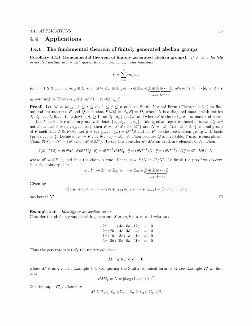
4.4. APPLICATIONS 55
4.4 Applications
4.4.1 The fundamental theorem of finitely generated abelian groups
Corollary 4.4.1 (Fundamental theorem of finitely generated abelian groups) If A is a finitelygenerated abelian group with generators x1, x2,. . ., xn. and relations
0 =
n∑
j=1
mi,jxj
for i = 1, 2, 3, . . . ,m, mi,j ∈ Z, then A ∼= Zd1⊕ Zd2
⊕ · · · ⊕ Zdt⊕ Z⊕ Z⊕ · · ·Z︸ ︷︷ ︸
m−t times
, where d1|d2| · · · |dt and are
as obtained in Theorem 4.3.1, and t = rank([mi,j ]).
Proof. Let M = [mi,j ], 1 ≤ i ≤ m, 1 ≤ j ≤ n and use Smith Normal Form (Theorem 4.3.1) to findunimodular matrices P and Q such that PMQ = [∆, Z] = D, where ∆ is a diagonal matrix with entriesd1, d2, . . . , dt, 0, . . . , 0, satisfying d1 ≥ 1 and d1 | d2 | . . . | dt and where Z is the m by n−m matrix of zeros.
Let F be the free abelian group with basis x1, x2, . . . , xn. Taking advantage (or abuse) of linear algebranotation. Let ~x = (x1, x2, . . . , xn), then F = ~z · ~x : ~z ∈ Z
n and N = ~w ·M~x : ~w ∈ Zm is a subgroup
of F such that A ∼= F/N . Let ~y = (y1, y2, . . . , yn) = Q−1~x and let F ′ be the free abelian group with basisy1, y2, . . . , yn. Define θ : F → F ′, by θ(~z · ~x) = ~zQ · ~y. Then because Q is invertible, θ is an isomorphism.Claim θ(N) = N ′ = ~w′ ·D~y : ~w′ ∈ Z
m. To see this consider ~w ·M~x an arbitrary element of N . Then
θ(~w ·M~x) = θ(~wM · ~x)~wMQ · ~y) = ~wP−1PMQ · ~y = (~wP−1)D · ~y = (~wP−1) ·D~y = ~w′ ·D~y ∈ N ′
where ~w′ = ~wP−1, and thus the claim is true. Hence A = F/N ∼= F ′/N ′. To finish the proof we observethat the epimorphism
ϕ : F ′ → Zd1⊕ Zd2
⊕ · · · ⊕ Zdt⊕ Z⊕ Z⊕ · · ·Z︸ ︷︷ ︸
m−t times
Given by
ϕ(z1y1 + z2y2 + · · ·+ ztyt + zt+1yt+1 + · · ·+ znyn) = (z1, z2, . . . , zn)
has kernel N ′.
Example 4.4: Identifying an abelian groupConsider the abelian group A with generators X = a, b, c, d, e and relations
−2a +4c−6d−12e = 0−2a+2b −4c−4d −4e = 01a+1b −3c+1d +1e = 0−3a−3b+15c−9d−21e = 0
Thus the generators satisfy the matrix equation
M · (a, b, c, d, e) = 0,
where M is as given in Example 4.3. Computing the Smith canonical form of M see Example ?? we findthat
PMQ = D = [diag (1, 2, 6, 0) ,~0]
(See Example ??). Therefore
M ∼= Z1 ⊕ Z2 ⊕ Z6 ⊕ Z0∼= Z2 ⊕ Z6 ⊕ Z

56 CHAPTER 4. FINITELY GENERATED ABELIAN GROUPS
(Note: Zm = Z/mZ, hence Z1 = Z/Z ∼= 0 the trivial group and Z0 = Z/0Z ∼= Z.) Indeed
Q−1 · (a, b, c, d, e) = (a+ b− 3c+ d+ e, 2b− 5c− d− e,−b+ 3c− e, c, e)
and soH1 = 〈2b− 5c− d− e〉 ∼= Z2, H2 = 〈−b+ 3c− e〉 ∼= Z6,H3 = 〈c〉 ∼= Z are such thatM = H1+H2+H3
and H1 ∩H2 = H2 ∩H3 = H1 ∩H3 = 0. Thus M is the (internal) direct sum of the subgroups H1,H2 andH3.
Remarks:
Saying that P is an integer matrix with determinant ±1 is of course equivalent to P ∈ SLn(Z) or is unimodal.I found this proof in several sources. including Michael Artin’s book, Algebra, Prentice hall (1991) Chapter12 Theorem 4.3 on page 458.
4.4.2 Systems of Diophantine Equations
Corollary 4.4.2 Let M,P,Q,D be as in Theorem 4.3.1, ~b ∈ Zn and ~c = P~b. Then the following fourstatements are equivalent:
(1). The system of linear equations M~x = ~b has an integer solution
(2). The system of linear equations D~y = ~c has an integer solution
(3). For every rational vector ~u such that ~uM is an integer vector, the number ~u ·~b is an integer
(4). For every rational vector ~v such that ~vD is an integer vector, the number ~v · ~c is an integer.
Proof.
(1) ⇐⇒ (2): Observe that
M~x = ~b⇐⇒ (P−1DQ−1)~x = ~b⇐⇒ D(Q−1~x) = ~c⇐⇒ D~y = ~c,
where ~y = Q−1~x. Thus because det(Q) = ±1 implies det(Q−1) = ±1 we see that
~x ∈ Zn ⇐⇒ ~y = Q−1~x ∈ Zn.
(3) ⇐⇒ (4): Observe that
~vD ∈ Zn ⇐⇒ ~v(PMQ) ∈ Z
n ⇐⇒ (~vP )MQ ∈ Zn ⇐⇒ (~vP )M ∈ Z
nQ−1 = Zn ⇐⇒ ~uM ∈ Z
n,
where ~u = ~vP . Thus because det(P ) = ±1 we see that
~u ∈ Qm ⇐⇒ ~v ∈ Q
m,
and, by (3), ~u ·~b ∈ Z. But
~u ·~b ∈ Z ⇐⇒ (~vP )(P−1~c) ∈ Z⇐⇒ ~v · ~c ∈ Z.
Therefore (3) implies (4). Reversing the order of the argument, we get
~uM ∈ Zn ⇐⇒ ~vD ∈ Zn
and~v · ~c⇐⇒ ~u ·~b ∈ Z.
Therefore (4) implies (3).

4.4. APPLICATIONS 57
(2) ⇐⇒ (3): D~y = ~c implies ~v(D~y) = ~v ·~c for every ~v ∈ Qm, hence (~vD) ·~y = ~v ·~c. If ~vD ∈ Z
n, then ~v ·~c ∈ Z.Thus (2) implies (4). In order to prove that (4) implies (2), first we observe that
~c = (c1, . . . , cs, 0, . . . , 0).
For suppose cj 6= 0, j > s. Consider
~v = (0, . . . , 0, 1/(2cj), 0, . . . , 0),
where 1/(2cj) appears in the j-th position. Because ~vD = 0 ∈ Zn, then by (4) ~v ·~c = 1/2 ∈ Z, and we
arrive at a contradiction. Thus cj = 0 for j > s. Next, for i = 1, . . . , s, we consider vectors
vi = (0, . . . , 0, 1/di, 0, . . . , 0).
Because viD ∈ Zn , then by (4), vi~c ∈ Z and hence ci/di ∈ Z. Let
~y = (y1, . . . , ys, 0 . . . , 0),
where yi = ci/di , i = 1, . . . , s. Then ~y ∈ Zn , and D~y = ~c.
Remarks:
The proof of Corollary 4.4.2 came from Felix Lazebnik, On Systems of Linear Diophantine Equations, TheMathematics Magazine, vol. 69, no. 4, October 1996, 261–266.
If ~u ∈ Zm is a vector, then by gcd (~u) we mean the greatest common divisor of the the entries in ~u.
Corollary 4.4.3 The m by n system of Diophantine equations M~x = ~b has a solution ~x ∈ Zn if and only if
gcd (~yM) divides ~y ·~b for every vector ~y ∈ Zm.
We provide two proofs.
First proof. Suppose M~x = ~b has integral solution ~x and that ~b ∈ Zm. If g divides each entry of ~yM ,
then g divides the integral linear combination (~yM) · ~x = ~y · (M~x) = ~y ·~b.Conversely suppose gcd (~yM) divides ~y · ~b for every vector ~y ∈ Zm and let ~u ∈ Qm be such that~uM ∈ Z
n. Let 0 < δ ∈ Z be such that ~y = δ~u ∈ Zm. Then because ~uM ∈ Z
m, we see thatδ gcd (~uM) = gcd (δ~uM) = gcd ((δ~u)M) divides δ~u ·~b. That is the integer
δ~u ·~b = Rδ gcd (~uM)
for some integer R. Hence~u ·~b = R gcd (~uM) ∈ Z.
Thus Statement (3) of Corollary 4.4.2 holds and therefore so does Statement (4).
Second proof. According to Statements (1) and (2) of Corollary 4.4.2,M~x = ~b has has an integer solution~x if and only if D~y = ~c has an integer solution ~y. The latter is uncoupled and has solution ~y =(y1, y2, . . . , yn) if and only if diyi = ci, for i = 1, 2, . . . , n. For a fixed i and a fixed prime p, thisequation has a solution modulo p if and only if gcd (di, p) divides ci. Hence if this equation has a
solution modulo p for all primes p, then si must divide ci, or equivalently D~y = ~b has an integersolution ~y. The converse is easier. You can use the integer solution to give you a solution For everyprime p.
58 CHAPTER 4. FINITELY GENERATED ABELIAN GROUPS
Remarks:
The second proof was received by e-mail communication from Bryan Shader.
4.4.3 Exercises
1. Show that every integer matrix M has a unique Smith normal form.
2. Compute the Smith normal form of the matrix
M =
2 4 −4 −2−4 −12 12 82 −4 4 6
3. Let A be the abelian group with presentation
A = 〈a, b, c, d : 2a+ 4b− 4c− 2d = 0,−4a− 12b+ 12c+ 8d = 0, 2a− 4b+ 4c+ 6d = 0〉 .
What is the canonical decomposition for A.
4. Let Γ be a graph, set g = gcd (deg(u) : u ∈ V (Γ)) and choose positive integer n satisfying
(n
2
)
≡ 0 (mod |E(Γ)|) (4.3)
n− 1 ≡ 0 (mod g) . (4.4)
Let B be the set of subgraphs of the complete graph Kn that are isomorphic to Γ and define the matrix
M : E(Kn)× B → 0, 1
by
M [e, Y ] =
1 if e ∈ E(Y );0 if e /∈ E(Y )
.
(a) Show that there is an integer valued vector ~x such that M~x = J , where J [X ] = 1, for all X ∈ B.(b) Show that M has constant row sum c for some positive integer c.
(c) Show that there is a constant λ and a positive integer valued vector ~y such that M~y = λJ .
(d) Conclude that the complete multi-graph λKn can be edge decomposed into subgraphs isomorphicto X . (The multiigraph λKn has each edge repeated λ times.)

Chapter 5
Fields
5.1 A glossary of algebraic systems
Semigroup: A semigroup is a set with an associative binary operation.
Ring: A ring is a set with two binary operations, addition and multiplication, linked by the distributivelaws:
a(b + c) = ab+ ac
(b + c)a = ba+ ca
Rings are abelian groups under addition and are semigroups under multiplication. We will assume ourrings have the multiplicative identity 1 6= 0.
Commutative ring: A commutative ring is a ring in which the multiplication is commutative.
Domain: A domain (or integral domain) is a ring with no zero divisors, that is
ab = 0⇒ a = 0 or b = 0 for all a, b in the domain .
Field: A field is a commutative ring in which every nonzero element has a multiplicative inverse.
Skew field: A skew field (or division ring) is a ring (not necessarily commutative) in which the nonzeroelements have a multiplicative inverse. The quaternions
Q = 1 + ai+ bj + ck : a, b, c ∈ R
where ij = k,jk = i,ki = j,and i2 = j2 = k2 = −1 is an example of a skew field.
R-module: If R is a commutative ring then an abelian group M is an R-module if scalar multiplication(r,m) 7→ rm is also defined such that for all r, s ∈ R and m,n ∈M :
(r + s)m = rm+ sm
(m+ n)r = mr + nr
(rs)m = r(sm)
1R ·m = m
Vector Space: A vector space is an R-module where R is a field.
59

60 CHAPTER 5. FIELDS
Euclidean Domain A domain D with a division algorithm is called a Euclidean Domain (ED).
By a division algorithm on a domain D we mean there is a function
deg : D 7→ 0 ∪ N
such that if a, b ∈ D and b 6= 0 then there exists q, r ∈ D such that a = qb + r where either r = 0 ordeg(r) < deg(b).
Example 5.1: Euclidean Domain Two examples of Euclidean Domains are:
1. Z with deg(x) = |x|2. F[x] the set of all polynomials in x whose coefficients are from the field F with deg(f(x)) the
degree of the polynomial f(x).
5.2 Ideals
Definition 5.1: A subset I of a ring R is an ideal if
1. if a, b ∈ I, then a+ b ∈ I,
2. if r ∈ R and a ∈ I, then ra ∈ I and ar ∈ I
We write I ⊳ R and say I is an ideal of R.
A function f : R→ S is a homomorphism of the rings R,S if for all a, b,∈ R
f(a+ b) = f(a) + f(b)
f(ab) = f(a)f(b)
If f is a homomorphism, then the kernel (f) = x ∈ R : f(x) = 0.
Proposition 5.2.1 The kernel of a ring homomorphism is an ideal.
Proof. Let f : R → S be a homomorphism of rings. If a, b ∈ kernel (f) then f(a + b) = f(a) + f(b) =0 + 0 = 0 ⇒ a + b ∈ kernel (f). If a ∈ kernel (f) and r ∈ R then f(ar) = f(a)f(r) = 0 · f(r) = 0. Thusra ∈ kernel (f). Similarly ra ∈ kernel (f). Therefore kernel (f) ⊳ R.
If I ⊳ R then we may define the factor ring R/I whose elements are the cosets a+ I : a ∈ R of I andwhere we define addition and multiplication by
(a+ I) + (b+ I) = (a+ b) + I
(a+ I)(b + I) = ab+ I
Note that f : R 7→ R/I given by f(a) = a+ I is a homomorphism with kernel I. Thus
the study of homomorphisms is equivalent to the study of ideals.
The ideal of R generated by x1, x2, ..., xt ∈ R is (x1, x2, ..., xt) and is the intersection of all ideals thatcontains x1, x2, ..., xt. If R is commutative and 1 ∈ R then (x1, x2, ..., xt) = a1x1 + a2x2 + ... + atxt :a1, a2, ..., at ∈ R.
Definition 5.2: An ideal I that is singularly generated, i.e. I = (a), is called a principle ideal .

5.3. THE PRIME FIELD 61
Definition 5.3: A ring with only principle ideals is called a principle ideal ring (PIR).
And similarly a domain with only principle ideals is a principle ideal domain (PID).
Theorem 5.2.2 If R is a Euclidean Domain, then R is a principle ideal domain.
Proof. Let R be a Euclidean Domain and let deg be the degree function for R. Suppose I ⊳ R, choosea ∈ I, a 6= 0 to have the smallest degree. If b ∈ I write b = aq+r where q, r ∈ R and r = 0 or deg(r) < deg(a).But then r = b − aq ∈ I so deg(r) < deg(a) is impossible and thus r = 0 and b = aq ∈ (a). Hence I ⊆ (a)and therefore I = (a).
Conversely not every PID is an ED.
Some examples of PIDs are Z and F[x]. For example in Z, the ideal (a, b) = (g) where g = gcd (a, b).Thus it is common to drop the prefix and just write (a, b) for the greatest common divisor of a and b.
Definition 5.4: An ideal P is a prime ideal , if whenever ab ∈ P , then either a ∈ P or b ∈ P .
For example the prime ideals of Z are (p) = pZ = xp : x ∈ Z, where p is prime integer.
Theorem 5.2.3 0 6= P ⊳ R is a prime ideal if and only if R/P is a domain.
Proof. Suppose R = R/P is a domain. Denote α by α = a+ P ∈ R. If αβ = 0, then α = 0 or β = 0 butαβ = αβ by definition of multiplication so translating to R we see that αβ ∈ P ⇒ α ∈ P or β ∈ P so P is aprime ideal.
Conversely, if P prime ideal, then αβ ∈ P ⇒ α ∈ P or β ∈ P . Thus αβ = 0⇒ α = 0 or β = 0. Hence Rcan have no zero divisors and thus R is a domain.
5.3 The prime field
Definition 5.5: A prime field is a field with no proper subfields.
Theorem 5.3.1 Every prime field Π is isomorphic to Zp or Q.
Proof. Let 1 be the multiplicative identity of Π and set R = n ·1 : n ∈ Z ⊂ Π. It is easy to see that Π is adomain. The map θ : Z→ R given by n 7→ n · 1 is a homomorphism of rings and is onto. Let P = kernel (θ),then R = Zp because R is a domain by the previous theorem P is a prime ideal of Z. Thus P = 0 orP = (p), p a prime.
If P = 0 then Z ∼= R and therefore Π ⊇ S where S ∼= Q. But it has no proper subfields so Π = S ∼= Q.If P = (p) then R ∼= Zp and therefore Π ∼= Zp.
Theorem 5.3.2 Every field F contains a unique prime field Π.
Proof. Let Π be the intersection of all subfields of F, 1 ∈ F so Π 6= 0. This is a subfield having no propersubfields. Therefore Π is a prime field and is clearly unique.
Definition 5.6: If the prime field of F is Π ∼= Zp we say F has characteristic p otherwise we say F hascharacteristic 0.

62 CHAPTER 5. FIELDS
Theorem 5.3.3 Every finite field F has pn elements for some prime p and natural number n.
Proof. F is a finite dimensional vector space over its prime field Π. Then |F| = |Π|dimΠF = pn wheren = dimΠF.
Theorem 5.3.4 The commutative ring R is a field if and only if R contains no proper ideals.
Proof. Suppose R is a field and let a ∈ R, a 6= 0, then 1 = a−1a ∈ (a)⇒ R ⊆ (a)⇒ R = (a). Thus R hasno proper ideals.
Conversely suppose R contains no proper ideal. Then for all a 6= 0, (a) = R. Hence 1 ∈ (a)⇒ 1 = ra forsome r ∈ R and so a has an inverse and therefore R is a field.
Definition 5.7: An ideal M of R is a maximal ideal if there is no ideal I ⊳ R such that M 6= R andthere is no proper ideal of R that contains I
Theorem 5.3.5 M is a maximal ideal of the commutative ring R if and only if R/M is a field.
Proof. M ⊳ R is a maximal ideal if and only if by the law of correspondence R has no ideals if and only ifby Theorem 5.3.4 R/M is a field.
Corollary 5.3.6 Maximal ideals of commutative rings are prime ideals.
Proof. If M ⊳ R is a maximal ideal, then R/M is a field but fields are domains so therefore M is primeideal.
Theorem 5.3.7 Every prime ideal of a PID is a maximal ideal.
Proof. Let R be a PID and suppose P is a prime ideal of R. Let I ⊳ R such that P ⊳
6= I ⊳
6=R. Because R
is a PID we may choose p, a ∈ R such that P = (p) and I = (a). Then p ∈ (a), so p = ra for some r ∈ R.Thus because P is a prime ideal either r ∈ (p) or a ∈ (p). But if a ∈ (p) then I = (a) ⊆ (p) = P which isa contradiction. Thus r ∈ (p) so r = sp for some s ∈ R and therefore p = spa so p(1 − a) = 0. Thereforesa = 1 because p 6= 0 and R is a domain. Therefore 1 ∈ (a)⇒ I = (a) = R which is a contradiction. HenceP is maximal. (There are no proper ideals of R that properly contain P .)
An element u ∈ R is called a unit if it has an inverse. The units of Z are ±1. In a field F every non-zeroelement is a unit. In F[x] the constant polynomials are the units.
Definition 5.8: An element p ∈ R is an irreducible if and only if in every factorization p = ab eithera or b is a unit. If p = uq where u is a unit then p and q are said to be associates .
Theorem 5.3.8 If R is a PID then the non-zero prime ideals are the ideals (p), where p is irreducible.
Proof. Suppose (p) 6= 0 is a prime ideal of R and let p = ab be a factorization in R then either a ∈ (p) orb ∈ (p). Say a ∈ (p), then a = sp for some s. Hence p = spb⇒ p(1 − sb) = 0⇒ sb = 1, because p 6= 0, andR is a domain. Therefore b is a unit and hence p is irreducible.
Corollary 5.3.9 If R is PID and p ∈ R is irreducible, then R/P is a field.
Proof. p irreducible ⇒ by Theorem 5.3.8 that (p) is a prime ideal. Therefore by Theorem 5.3.7 (p) is amaximal ideal. Consequently by Theorem 5.3.5 R/P is a field.
5.3. THE PRIME FIELD 63
Lemma 5.3.10 If F is a field and f(x) is irreducible in F[x] then
F[x]/(f(x))
is a field containing a root of f(x) and a subfield isomorphic to F.
Proof. If f(x) is irreducible then F = F[x]/(f(x)) is a field. Let R = F[x] and I = (f(x)) so F = R/I. Iff(x) = a0 + a1x+ a2x
2 + ...+ anxn then
f(x+ I) = a0 + a1(x + I) + a2(x + I)2 + ...+ an(x + I)n
= a0 + a1x+ a2x2 + ...+ anx
n + I
= f(x) + I = I, because f(x) ∈ I.
Therefore f(x+ I) is the zero of F . Hence x+ I in F is a root of f(x) and x+ I : x ∈ F is a subfield of Fisomorphic to F.
Corollary 5.3.11 (Galois) If f(x) is an irreducible polynomial of degree n in Zp[x], then F = Zp[x]/(f(x))is a finite field of order pn.
Proof. The distinct cosets of I = (f(x)) are g(x) + I where deg g(x) < deg f(x) and there are pn of such.
If h(x) ∈ Zp[x], then write h(x) = g(x)f(x) + r(x) where r(x) = 0 or deg r(x) < deg f(x). Thenh(x) − r(x) = g(x)f(x) ∈ (f(x)) = I. So h(x) ∈ r(x) + I and therefore h(x) + I = r(x) + I.Hence r(x) = a0 + a1x+ a2x
2 + ...+ an−1xn−1.
5.3.1 Exercises
1. If f(x) = a0 + a1x+ a2x2 + · · ·+ anx
n is a polynomial with coefficients a0, a1, a2, . . . , an in the field F,then we define the derivative of f(x) to be the polynomial f ′(x) = a1 + a22x+ · · ·+ annx
n−1. Showthat f(x) ∈ F[x] has a repeated root if and only if (f(x), f ′(x)) is a non-zero proper ideal of F[x].
2. Let F be a field of characteristic p > 0. Show that
(a+ b)pk
= apk
+ bpk
for all a, b ∈ F and non-negative integer k.

64 CHAPTER 5. FIELDS
5.4 algebraic extensions
If the field L contains the subfield K, we say that L is an extension of K, in this case L is a vector spaceover K. The degree of the extension of L over K is [L : K] the dimension of L as a vector space over K. Afield L is a finite extension of a field L if [L : K] is finite. Following the theory of vector spaces it is easy tosee that if F ⊂ K ⊂ L is an extension of fields that
[L : F] = [L : K] [K : F] (5.1)
If K is an extension of the field F, and α1, α2, . . . , αk ∈ K, then the smallest field that contains F andα1, α2, . . . , αk is denoted by
K = F(α1, α2, . . . , αn)
and we say K arises form F by the adjunction of α1, α2, . . . , αn.If K is an extension of the field F, then an element α ∈ K is algebraic over F if α is a root of a polynomial
f(x) ∈ F[x]. Among all polynomials that have α as a root choose m(x)
m(x) = m0 +m1x+m2x2 + · · ·mk−1x
k−1 +mkxk
to be one that has smallest degree. Furthermore, because m−1k m(α) = 0, we may choose mk = 1. This
uniquely defines m(x) and we call this polynomial the minimal polynomial .Suppose m(x) is the minimal polynomial of α and f(x) is any polynomial that has α as a root. Using
the division algorithm we may writef(x) = q(x)m(x) + r(x),
where r(x) = 0 or deg(r(x)) < deg(m(x)). But the latter is impossible, because m(x) is the minimalpolynomial of α. Therefor m(x) divides f(x) in F[x]. Hence in particular, if α is a root of the irreduciblepolynomial f(x), then f(x) and m(x) are associates, and deg(f(x)) = deg(m(x)) = k. It follows that
1, α, α2, α3 + . . . , αk−1
are linearly independent, because any linear dependence
h(α) = h0 + h1α+ h2α2 + h3α
3 + . . . hk−1αk−1 = 0,
is a contradiction to the minimality of m(x). Consider the ring
F(α) = f(α) : f(x) ∈ F[x]
and ring homomorphism θ : F[x]→ F(α). The kernel is
ker θ = f(x) ∈ F[x] : f(α) = 0 = (m(x))
ThusF(α) ∼= F[x]/(m(x))
is a field extension over F of degree k = deg(m(x)), the minimal polynomial of α over F. It is now easyto see that if α and β are roots of the irreducible polynomial f(x) ∈ F[x], then F(α) ∼= F(β). In the nexttheorem we show that there is an isomorphism that maps α to β.
Theorem 5.4.1 Let α and β be roots of the irreducible polynomial f(x) ∈ F[x], then there is an isomorphismθ : F(α)→ F(β) such that θ(α) = β.
Proof. Let n = deg(f(x)), then The elements of F(α) are of the form
a0 + a1α+ a2α2 + · · ·+ an−1αn−1

5.5. SPLITTING FIELDS 65
and we operate with them using the relation f(α) = 0. Similarly the elements of F(β) are of the form
a0 + a1β + a2β2 + · · ·+ an−1βn−1
and we operate with them using the relation f(β) = 0. Thus the mapping θ, where
θ : a0 + a1α+ a2α2 + · · ·+ an−1αn−1 → a0 + a1β + a2β
2 + · · ·+ an−1βn−1
is the required isomorphism.
An extension field K of F is said to be algebraic over F if every element of K is algebraic over F.
Theorem 5.4.2 Every finite extension K of the field F is algebraic and may be obtained by the adjunctionof a finite number of algebraic elements and conversely.
Proof. If n = [K : F] is the degree of the extension and α ∈ K, then
1, α, α2, α3, . . . , αn−1
are linearly independent and thus there exist coefficients h0, h1, . . . , hn−1 ∈ F such that
h(α) = h0 + h1α+ h2α2 + · · ·+ hn−1α
n−1 = 0.
Therefore α is algebraic over F, and consequently K is an algebraic extension. Moreover choosing a basisα1, α2, . . . , αn of K as a vector space over F. We see that
K = F(α1, α2, . . . , αn).
Conversely the adjunction of an algebraic element α1 gives rise to an algebraic extension F(α1) over F ofdegree deg(m(x) over F, where m(x) is the minimal polynomial of α1 over F. By Equation (5.1) we see thatthe successive extensions
F(α1),F(α1, α2),F(α1, α2, α3), . . .F(α1, α2, . . . , αk)
of algebraic elements α1, α2, α3, . . . , αk is a sequence of finite algebraic extensions.
5.5 Splitting fields
If the polynomial f(x) ∈ F[x] completely factors into linear factors
f(x) = (x− α1)(x− α2) · · · (x − αn)
in the extension field K of F we say that f(x) splits over K. If f(x) splits over K and there is no subfield ofK over which f(x) splits, then K is called the splitting field of f(x) over F.
Theorem 5.5.1 If F is a field and f(x) ∈ F[x], then there exists a splitting field of f(x) over F.
Proof. Letf(x) = (x− α1)(x− α2) · · · (x − αr)g1(x)g2(x)g3(x) · · · gs(x)
be a factorization of f(x) into irreducible factors in F[x]. Where gi is not linear for i = 1, 2, . . . s. Letβ1 = αr+1 be a root of g1, then
F1 = F(β1) ∼= F[x]/(g1(x))
is a field in which g1 (and therefore f(x) ) splits off the linear factor (x − αr+1). Hence over F1, f(x) has afactorization into irreducibles
f(x) = (x− α1)(x − α2) · · · (x− αr)(x − αr+1)(x− αr+2) · · · (x− αr′)g′1(x)g
′2(x)g
′3(x) · · · g′s′(x).
Now we may choose a root β2 = αr′+1 of g′1(x) and form F2 = F1(β2) = F(β1, β2) and split off from f(x) thelinear factor (x − β2). Continuing in this fashion we arrive at a field Fs = F(β1, β2, . . . , βs) in which f(x)completely factors into linear factors.
It follows from Theorem 5.4.1 that any two splitting field of a polynomial are isomorphic.

66 CHAPTER 5. FIELDS
5.6 Galois fields
Finite fields are also know as Galois fields . Recall that every finite field F is a vector space over its primefield Π. Thus if the characteristic of Π is the prime integer p, then |F| = pn where n = [F : Π].
Theorem 5.6.1 For all primes p and positive integers n, all fields of order pn are isomorphic.
Proof. Let q = pn, and suppose F is a field of order q. then F \ 0 is an abelian group of order q− 1.Henceαq−1 = 1 for every α ∈ F \ 0. Then upon multiplying by q, we see that every element α ∈ F satisfies
αq − α = 0.
Hence every element of F is a root of the polynomial f(x) = xq − x. Then minimal polynomial of αi ∈ F
over Π is (x− αi) and thus (x− αi) must divide f(x) and therefore
f(x) = (x− α1)(x− α2) · · · (x − αn)
because the degree of the later is also q. Thus F = Π(α1, α2, . . . , αn) is the splitting field of f(x) and istherefore uniquely determined up to isomorphism.
Now that we have Theorem 5.6.1 we may adopt the notation Fq, for the unique (up to isomorphism) finitefield of order q, where q is a prime power.
5.7 Constructing a finite field
By constructing a finite field of order pn we mean find an irreducible polynomial over Zp of degree n and agenerator α for the cyclic group of non-zero elements. Through out let p be a prime and n > 0 an integer.The divisor d of k is a maximal proper divisor of k, if d 6= k and there is no d < ℓ < k such that d ℓ ℓ. k.
Algorithm 1 to construct Fpn
Find f(X) ∈ Zp[X ] irreducible of degree nGeneratorFound← falsewhile not GeneratorFound
do
Randomly pick α = α(X) ∈ Zp[X ] monic of degree < ncomment:Assume α is indeed a generator
GeneratorFound← truefor each maximal proper divisor d of pn − 1
do
k ← (pn − 1)/dβ ← αk ”Use the power algorithm”if β = 1 then GeneratorFound← false
5.7. CONSTRUCTING A FINITE FIELD 67
Algorithm 2 to construct Fpn a refinement of Algorithm 1
IrreducibleFound← falsewhile not IrreducibleFound
do
Randomly pick f(X) ∈ Zp[X ] monic of degree nGeneratorFound← falsewhile not GeneratorFound
do
Randomly pick α = α(X) ∈ Zp[X ] monic of degree < nGeneratorFound← truefor each maximal proper divisor d of pn − 1
do
k ← (pn − 1)/dβ ← αk ”Use the power algorithm”if β = 1 then GeneratorFound← false
β ← α(pn−1) ”Use the power algorithm”if β = 1 then IrreducibleFound← true
The Power Algorithm
β ← 1E ← α
while n 6= 0 do
if n is odd then β ← β ∗ EE ← E ∗ En← n/2 ”Integer division”
. . . . . . . . . . . . . . . . . . . . . . . . . . . . . . . . . . . . . . . . . . . . . . . . . . . . . . . . . . . . . . . . . . . . . . . . . . . . . . . . . . . . . . . . . . . . . . . . . . . . . . . . . .
5.7.1 Exercises
1. Determine the minimal polynomial of of α = 3√2−√5 over the field Q of rationals.
2. Construct the finite field F81 by finding an irreducible polynomial f(x) over Z3 such that F81∼=
Z3[x]/(f(x)) and find a generator α for the multiplicative group of non-zero elements in F. Find j,0 ≤ j < 80 such that (α2 + α3)(α + 1) = αj .

68 CHAPTER 5. FIELDS

Chapter 6
Linear groups
6.1 The linear fractional group and PSL(2, q)
Let Fq be the finite field of order q and let X = Fq ∪ ∞ (the so-called projective line). A mappingf : X → X of the form
x 7→ ax+ b
cx+ d
where a, b, c, d ∈ Fq,1∞ = 0, ∞1 = ∞, 1 − ∞ = ∞,∞ − 1 = ∞ and ∞
∞ = 1 is called a linear fractionaltransformation. The determinant of f is
det f = ad− bcThe set of all linear fractional transformations whose determinant is a non-zero square is LF(2, q), the linearfractional group.
Theorem 6.1.1 LF(2, q) is a group.
Proof. Let f, g ∈ LF(2, q), then
f : x 7→ ax+bcx+d and g : x 7→ ux+v
wx+z
for some a, b, c, d, u, v, w, z ∈ Fq, and det f and det g are non-zero squares. Then
fg(x) =
a
(
ux+ v
wx + z
)
+ b
c
(
ux+ v
wx + z
)
+ d
=av + aux+ bwx + bz
cv + cux+ dwx + dz=
(au+ bw)x + av + bz
(cu + dw)x + cv + dz
and
det(fg) = (au+ bw)(cv + dz)− (av + bz)(cu+ dw)
= aucv + audz + bwcv + bwdz − aucv − avdw − bzcu− bwdz= aduz + bcvw − advw − bcuz= (ad− bc)(uz − vw) = (det f)(det g)
Therefore, because the product of two squares is a square, it follows that LF(2, q) is closed under functioncomposition. If
f : x 7→ ax+ b
cx+ d
69

70 CHAPTER 6. LINEAR GROUPS
is in LF(2, q), then det f = ad− bc is a non-zero square. Thus
g : x 7→ dx− b−cx+ a
has det g = ad− bc = det f is also a non-zero square and hence g ∈ LF(2, q). We compute fg.
(fg)(x) =
a
(
dx− b−cx+ a
)
+ b
c
(
dx− b−cx+ a
)
+ d
=adx− ab− bcx+ ba
cdx− cb− cdx+ ad=
(ad− bc)x(ad− bc) = x
Thus every f ∈ LF(2, q) has an inverse g ∈ LF(2, q). Therefore, LF(2, q) is a group of permutations on X
The general linear group GL(2, q) is the set of all 2 by 2 invertible matrices with entries in Fq. Thenormal subgroup of GL(2, q) consisting of all matrices with determinant 1 is called the special linear groupand is denoted by
SL(2, q) = M ∈ GL(2, q) : detM = 1.The center of SL(2, q) is Z = I,−I. The projective special linear group is PSL(2, q) = SL(2, q)/Z. Wenow show that the linear fractional group is isomorphic to the projective special linear group.
Theorem 6.1.2 LF(2, q) ∼= PSL(2, q)
Proof. Define Φ : SL(2, q)→ LF(2, q) by
φ :
[a bc d
]
7→(
x 7→ ax+ b
cx+ d
)
.
We show that Φ is an epimorphism with kernel Z = ±I. First, as onto is not immediately apparent, leta, b, c, d ∈ Fq where (ad− bc) = r2, r ∈ Fq, and r 6= 0. Then
Φ
([(a/r) (b/r)(c/r) (d/r)
])
=(a/r)x + (b/r)
(c/r)x + (a/r)=ax+ b
cx+ d
And therefore Φ is onto. To see that it is a homomorphism, we verify
Φ
([a bc d
] [u vw z
])
= Φ
([a bc d
])
Φ
([u vw z
])
. (6.1)
The left hand side of Equation (6.1) maps x to
(au+ bw)x + av + bz
(cu+ dw)x + cv + dz
and the right hand side of (6.1) maps x to
a
(
ux+ v
wx+ z
)
+ b
c
(
ux+ v
wx+ z
)
+ d
=av + aux+ bwx+ bz
cv + cux+ dwx + dz=
(au+ bw)x+ av + bz
(cu+ dw)x + cv + dz

6.1. THE LINEAR FRACTIONAL GROUP AND PSL(2, Q) 71
The kernel of Φ consists of those matrices M =
[a bc d
]
∈ SL(2, q), where
ax+ b
cx+ d= x.
Thus ax+b = cx2+dx. Consequently a = d and b = c = 0. But detM = ad−bc = 1, becauseM ∈ SL(2, q).Thus a2 = 1 and so a = ±1. Therefore Z = kerΦ and hence by the first law of homomorphisms,
PSL(2, q) = SL(2, q)/Z ∼= LF(2, q)
Corollary 6.1.3 |LF(2, q)| = q3 − q2
Proof. We know from Theorem 6.1.2 that LF(2, q) ∼= PSL(2, q) = SL(2, q)/Z . Thus
|LF(2, q)| = 1
2|SL(2, q)|.
The determinant mapdet : GL(2, q)→ F
⋆q
is an epimorphism with kernel SL(2, q). So,
|GL(2, q)| = (q − 1)|SL(2, q)|
The elements of GL(2, q) are 2 by 2 matrices that have non-zero determinant. The columns thus an orderedpair of linearly independent vectors in F
2q . The first column can be any vector except the zero vector and
there are q2 − 1 of these. The second column is any vector that is not a multiple of the first column. Thereare q2 − q such vectors. Hence
|GL(2, q)| = (q2 − 1)(q2 − q) = (q3 − q)(q − 1)
Therefore,|SL(2, q)| = q3 − q
and the result follows.
Lemma 6.1.4 LF(2, q) is isomorphic to the group
J =
x 7→ Ax +B
Bqx+Aq: Aq+1 −Bq+1 = 1 ; A,B ∈ Fq2
Proof. Let α be a primitive root of Fq2 and set
S =
[αq α−1 −1
]
The determinant detS = αq−α is non-zero because α is not in the subfield Fq of Fq2 . This S is non-singular.
Define Φ : SL(2, q)→ SL(2, q) byΦ :M 7→ S−1MS

72 CHAPTER 6. LINEAR GROUPS
Because S is non-singular the mapping Φ is an isomorphism. Let
g =
[a bc d
]
∈ SL(2, q).
Then
Φ(g) = S−1MS
=1
α− αq
[−1 −α1 αq
] [a bc d
] [αq α−1 −1
]
=1
α− αq
[−a− cα −b− dαa+ cαq b+ dαq
] [αq α−1 −1
]
=1
α− αq
[−aαq + b− cαq+1 + dα −aα+ b− cα2 + dαaαq − b+ cα2q − dαq aα− b+ cαq+1 − dαq
]
=
−aαq + b− cαq+1 + dα
α− αq
−aα+ b− cα2 + dα
α− αq
aαq − b+ cα2q − dαq
α− αq
aα− b+ cαq+1 − dαq
α− αq
Because if x ∈ Fq, then xq = x and (α− αq)q = αq − αq2 = αq − α = −(α− αq). Thus
Φ(g) =
[A BBq Aq
]
, (6.2)
where
A =−aαq + b− cαq+1 + dα
α− αq, and B =
−aα+ b− cα2 + dα
α− αq.
Thus every element of SL(2, q) has the form given in Equation (6.2). We now show that the number ofmatrices of this form that have determinant 1 = Aq+1 − Bq+1 is q3 − q = |SL(2, q)|. First suppose A = 0,Then B is a root of the polynomial Bq+1 = −1. A polynomial of degree (q + 1) has at most q + 1 distinctroots and thus there are at most q + 1 choices of B ∈ Fq2 such that Aq+1 − Bq+1 = 1, when A = 0. Foreach of the remaining q2 − q − 1 choices for B there are most q + 1 choices for A because each is a root ofthe polynomial Aq+1 = 1+Bq+1, which has at most q+1 roots. Therefore the number of matrices over Fq2
have the form given in Equation (6.2) with Aq+1 −Bq+1 = 1 is at most
(q3 − q − 1)(q + 1) + (q + 1) = (q2 − q)(q + 1) = q3 − q.
But Φ is an isomorphism, so there are at least |SL(2, q)| = q3 − q of them. Therefore
SL(2, q) ∼= Γ =
[A BBq Aq
]
: Aq+1 −Bq+1 = 1, A,B ∈ Fq2
.
Consequently
LF (2, q) = SL(2, q)/Z ∼= SL(2, q)/Z ∼= J.

6.1. THE LINEAR FRACTIONAL GROUP AND PSL(2, Q) 73
6.1.1 Transitivity
Lemma 6.1.5 Let G = LF(2, q), q = pe, p prime.
1. The stabilizer of ∞ is
G∞ = SAF(q) = x 7→ α2x+ β : α, β ∈ Fq, α 6= 0
and |G∞| = q(q − 1)/2.
2. The subgroup
H = x 7→ x+ β : β ∈ Fqis an Elementary Abelian subgroup of G∞ of order q in which the non-identity elements have order p.( In fact H ∼= Zp × Zp × · · · × Zp
︸ ︷︷ ︸
e times
. )
3. The subgroup G(0,∞) of G that fixes the two points 0 and ∞ is cyclic of order (q − 1)/2.
Proof.
1. First off, observe that if g(x) = α2x + β for some α, β ∈ Fq, α 6= 0. Then g(∞) = ∞ Thus g ∈ G∞.On the other hand if g(x) = ax+b
cx+d ∈ G∞ then
g(x) =a+ (b/x)
c+ (d/x)
so
∞ = g(∞) =a+ (b/∞)
c+ (d/∞)=a
c,
Thus c = 0. Therefore
g(x) =ax+ b
d
and ad = r2 for some r ∈ Fq, r 6= 0. Let α = a/r, α−1 = d/r. Then
g(x) =(a/r)x + (b/r)
(d/r)
=αx + (b/r)
α−1
= α2x+ α(b/r)
= α2x+ β
where β = α(b/r). Therefore
G∞ =x 7→ α2x+ β : α, β ∈ Fq, α 6= 0
There are q − 1 choices for a and q choices for b giving at most (q − 1)q possible elements of G∞. Butthere are duplicates,
α2x+ β = a2x+ b if and only if α = ±a and β = b.
Therefore
|G∞| =(q − 1)q
2.

74 CHAPTER 6. LINEAR GROUPS
2. Taking a = 1, we see that H ≤ G∞. There are q choices for β so
|H | = q = pe
If f(x) = x+ β, thenfp(x) = (f f · · · f)
︸ ︷︷ ︸
p times
(x) = x+ pβ = x,
because p = 0 in Fq. Thus every non-identity element has order p. Let f(x) = x+µ and g(x) = x+ η.Then
(fg)(x) = f(x+ η) = x+ η + µ = g(x+ µ) = (gf)(x).
Therefore H is Abelian.
3. Suppose f(x) ∈ G(0,∞), then f(∞) =∞ so f(x) = α2x+ β for some α, β ∈ Fq α 6= 0. By Part 2, Alsof(0) = 0 thus β = 0. Therefore
f(x) = α2x
and hence
G(0,∞) =x 7→ α2x : α ∈ Fq, α 6= 0
=⟨x 7→ ρ2x
⟩
Where ρ is a primitive element of Fq. Hence
|G(0,∞)| =q − 1
2
If G is a subgroup of Sym (Ω)) the symmetric group on Ω, then G acts on the k-permutations in a naturalway as follows:
g(S) = (g(s1), g(s2), . . . , g(sk)),
where S = (s1, s2, . . . , sk) is a k-permutation of Ω and g ∈ G. If this action is transitive on the set ofall k-permutations, then we say G is k-transitive. If for every pair of k-permutations S and T there is aunique g ∈ G such that g(S) = T , then we say that G is sharply k-transitive. The group G also acts on thek-element subsets of Ω in a natural way as follows:
g(S) = g(s1), g(s2), . . . , g(sk)
where S = s1, s2, . . . , sk is a k-element subset of Ω and g ∈ G. If this action is transitive on the set of allk-element subsets, then we say G is k-homogeneous. If for every pair of k-element subsets S and T thereis a unique g ∈ G such that g(S) = T , then we say that G is sharply k-homogeneous . Regardless if S is ak-permutation or a k-element subset the the orbit of S under the action of G is
OrbitGS = g(S) : g ∈ G,
and the stabilizer of S isGS = g ∈ G : g(S) = S.
We recall the Orbit Counting Lemma
Lemma 6.1.6 If G is a subgroup of Sym (Ω) and S is a point, a k-tuple or subset of Ω, then |OrbitGS| =|G|/|GS |.
Proposition 6.1.7 Let G = LF(2, q), X = Fq ∪ ∞.

6.1. THE LINEAR FRACTIONAL GROUP AND PSL(2, Q) 75
1. G is transitive on X.
2. G is 2-transitive on X.
3. (a) If q 6≡ 1 (mod 4), then G∞ is 2-homogeneous on X \ ∞.(b) If q ≡ 1 (mod 4), then G∞ has 2 orbits of unordered pairs.
4. (a) If q 6≡ 1 (mod 4), then G is 3-homogeneous on X \ ∞.(b) If q ≡ 1 mod 4, then G has 2 orbits of unordered triples.
Proof.
1. Using the Orbit Counting Lemma,
|OrbitG(∞)| = |G||G∞|
=(q3 − q)/2q(q − 1)/2
= (q + 1) = |X |.
Therefore G is transitive.
2. Using the Orbit Counting Lemma,
|OrbitG((0,∞))| = |G||G(0,∞)|
=(q3 − q)/2(q − 1)/2
= (q + 1)q.
This is the number of 2-permutations of X , therefore 2-transitive.
3. Let u, v ∈ X , u 6= v.
(a) If q ≡ 3 mod 4, then −1 is not a square. In which case v−u or u− v is a square If q ≡ 0 mod 2,
then q = 2e for some e and x = xq =(
x2e−1
)2
and thus every element is a square. Therefore
without loss we may assume that v− u = α2 for some nonzero α ∈ Fq. Let g(x) = α2x2 + u, theng ∈ G∞ and
g(0) = α2 · 0 + u = u
g(1) = α2 + u = v − u+ u = v
Therefore G is 2-homogeneous. (Note if q ≡ 0 mod 2, then G is in fact 2-transitive. )
(b) If q ≡ 1 mod 4, then either both v − u and u− v are squares or both are non squares. Let
A = u, v : u− v is a squareB = u, v : u− v is a non-square.
We now show both A and B are orbits under the action of G. The same proof as Part 3a showsthat A = OrbitG0, 1 otherwise let η ∈ Fq be a fixed non-square. If u, v ∈ Fq, u − v is not asquare, u 6= v then u−v
η = α2 for some α and we take
g(x) = α2x+ v.
Now g(0) = v and g(η) = α2η + v = u. Therefore B = OrbitG0, η.
4. Let a, b, c be a 3-element subset of X . Then by Part 1 there is a g1 ∈ G such that g1(a, b, c) =u, v,∞ for some v, v ∈ Fq, u 6= v.

76 CHAPTER 6. LINEAR GROUPS
(a) If q 6≡ 1 (mod 4), then by Part 3a there is a g2 ∈ G such that g2(u, v) = 0, 1. Clearly g2(∞) =∞. Therefore setting g = g2g1 we have g(a, b, c) = 0, 1,∞. Thus G is 3-homogeneous.
(b) If q ≡ 1 (mod 4), then we set η to be a fixed non-square and by Part 3b either there is a g2 suchthat g2(u, v) = 0, 1 or there is a g′2 such that g′2(i, v) = 0, η, but not both. Thus settingg = g2g1 or g = g′2g1 we find that g(a, b, c) = 0, 1,∞ or g(a, b, c) = 0, η,∞. Thus thereare two orbits of triples in this case.
6.1.2 The conjugacy classes
Proposition 6.1.8 In LF(2, q) only the identity map I : x 7→ x fixes (0, 1,∞).
Proof. Let G = LF(2, q) and suppose f ∈ G(0,1,∞). Then f ∈ G∞, so f(x) = α2x+ β. Also f(0) = 0 andf(1) = 1. Thus β = 0 and α2 = 1. Therefore f = I.
Proposition 6.1.9 Only I ∈ LF(2, q) fixes 3 or more points.
Proof. If
f(x) =ax+ b
cx+ d
fixes α ∈ Fq. Then α is a root of cx2 + (d − a)x + b. This quadratic has at most 2 distinct roots unlessc = (d− a) = b = 0 in which case f(x) = x, i.e., f = I.
If f(x) fixes∞, then f(x) = α2x+β, for some α, β ∈ Fq and x = α2x+β has at most one zero. Thereforef fixes at most 2 points.
Theorem 6.1.10 Let g be an element of order d in G. If g has a non-trivial k-cycle, then k = d.
Proof. Let g ∈ G be an element of order d, g 6= I, containing a k-cycle, then gk fixes at least k points.If k > 2, then g fixes at least 3 points, and by Proposition 6.1.9, g = I. Therefore k = d.Now assume g has 2-cycle (u, v). Then because G is 2-transitive, there exists f ∈ G such that f((0,∞)) =
(u, v). Then h = f−1gf contains the 2-cycle (0,∞). Write
h =ax+ b
cx+ d
where a, b, c, d ∈ Fq. Then h(0) = ∞ implies that d = 0 and h(∞) = 0 implies that a = 0. Thereforeh(x) = d/(cx).
h2(x) =d
c(d/(cx))=dcx
cd= x
And so h2(x) = I and d = 2.
Recall that the centralizer of g in the group G is
CG(g) = f ∈ G : fg = gfa subgroup of G. Also recall that the conjugacy class of g in G is
KG(g) = fgf−1 : f ∈ Gand because G acts on G via conjugation we have by the Orbit Counting Lemma that |KG(g)| = |G|/|CG(g)|.

6.1. THE LINEAR FRACTIONAL GROUP AND PSL(2, Q) 77
Theorem 6.1.11 Let G = LF(2, q), where q = pe and p is a prime.
1. G has at least q2 − 1 elements of order p, each of which fixes one point.
2. Let g ∈ H = x 7→ x+ β : β ∈ Fq. Then |CG(g)| = q.
3. (a) If q ≡ 1, 3 mod 4, then G has at least 2 conjugacy classes of elements of order p and these classeshave size (q2 − 1)/2 each.
(b) Otherwise, the field is of characteristic 2, and in this case G has at least 1 conjugacy class ofelements of order p and these classes have size q2 − 1.
Proof.
1. Suppose g has order p, then because there are 1 + q = 1 + pe points g must fix at least 1 point, andbecause g only has cycles of length p it cannot fix more than 1 point.
The group G is transitive, so for each α ∈ Fq we can set Hα = fHf−1 a subgroup of G of order q = pα
whose elements fix α. Each non-identity element of H has order p, because Hα ∼= H . The fact thatelements of order p fix only 1 point. shows that Hα ∩ Hβ = I for α 6= β. Therefore there existsq + 1 subgroups of G each containing q − 1 distinct elements of order p. Consequently there are atleast (q + 1)(q − 1) = q2 − 1 elements of order p in G.
2. Let g(x) = x+ β, β 6= 0, and f(x) = ax+bcx+d ∈ CG(g). Without loss we may assume ad− bc = 1. Then
x+ β = g(x) = (fgf−1)(x) =(1− acβ)x + α2β
−c2βx + (1 + acβ)
Therefore by Proposition 6.1.19, α2 = 1, and −c2 = 0, so c = 0 and ad = 1. Therefore
g(x) =ax+ b
cx+ d=a2x+ ab
acx+ ad= x+ ab ∈ H.
Therefore CG(g) ≤ H , but H is Abelian, so CG(g) = H and thus |CG(g)| = q.
3. Each element of Hα is conjugate to each element of H . So |CG(g)| = q for all g ∈ Hα and for allα ∈ Fq. Therefore the size |KG(g)| of the conjugacy class of g ∈ Hα is
|KG(g)| =|G||CG(g)|
=
q(q2 − 1)
q= (q2 − 1)/2 if q ≡ 1, 3 (mod 4)
q2 − 1 otherwise
Because there are at least q2− 1 such elements of order p there must be at least 2 conjugacy classes ofelements of order p, when q ≡ 1, 3 (mod 4) and at least 1 when q ≡ 0 (mod 4).
Let
ω = ω(q) =
1 if q ∼= 1 mod 2
2 if q ∼= 0 mod 2.
Then |G| = ω(q3 − q)/2 = 3ω(q+13
). Recall G is 2-transitive, so
|OrbitG((0,∞))| = q(q + 1) =|G|
|G(0,∞)|
and so |G0,∞| = ω(q − 1)/2.

78 CHAPTER 6. LINEAR GROUPS
Theorem 6.1.12 Let G = LF(2, q), q a prime power.
1. G has at least
1
4ωq(q + 1)(q − 1− 2/ω) =
q(q + 1)(q − 3)/4 if q is odd
q(q + 1)(q − 2)/2 if q is even
non-identity elements whose order d divides ω(q− 1)/2, d 6= 2, and these elements fix exactly 2 points.
2. Let g ∈ G(α,β) have order d 6= 1 dividing ω(q − 1)/2.
• If d 6= 2, then CG(g) = G(α,β) and is cyclic of order |CG(g)| = ω(q − 1)/2.
• If d = 22, then CG(g) ⊃ G(α,β) and is dihedral of order |CG(g)| = ω(q − 1).
3. Let d 6= 1 divide ω(q − 1)/2.
• If d 6= 2, then there exists at least φ(d)/2 conjugacy classes of elements of order d and they eachhave size ωq(q + 1).
• If d = 2, then there exists at least one conjugacy classes of elements of order 2 and it has sizeωq(q − 1)/2.
Proof. Let α, β ∈ X,α 6= β.
1. The 2-transitivity of implies that there exists f ∈ G such that f : (0,∞) 7→ (α, β). Thus G(α,β) =fG(α,β)f
−1, and so
|G(α,β)| = |G(0,∞)| =ω(q − 1)
2.
Thus because non-identity elements of G fix at most 2 points, we have
Gα,β ∩Gγ,δ = I.
for α, β 6= γ, δ. Therefore there exists at least
(q + 1
2
)
|G(0,∞)| =q + 1
2
( |G|(q + 1)q
− 1
)
=1
4q(q + 1)(ω(q − 1)− 2) =
1
4ωq(q + 1)(q − 1− 2/ω)
non-identity elements whose order divides ω(q − 1)/2.
2. Let g(x) ∈ G(0,∞), where g 6= I. Then g(x) = αx/α−1 for some α ∈ Fq, α2 6= 1. The subgroup G(0,∞)
is cyclic of order ω(q−1)/2 so G(0,∞) ⊆ CG(g). Conversely, suppose h(x) =ax+ b
cx+ d∈ CG(g). (Without
loss ad− bc = 1.) So h−1(x) =dx− b−cx+ d
and hgh−1 = g imply
(adα− bcα−1)x + bd(α− α−1)
ac(α−1 − α)x+ (adα−1 − bcα) =αx
α−1
and therefore
bd(α− α−1) = ac(α−1 − α) = 0.
Thus because α2 6= 1, it follows that bd = ac = 0. Consequently 0 ∈ b, d and 0 ∈ a, c. If neither aor nor d is zero, then b = c = 0 and hence h(x) = ax/d. Obviously h(x) ∈ G(0,∞).
6.1. THE LINEAR FRACTIONAL GROUP AND PSL(2, Q) 79
(a) If a = 0, then
αx
α−1=α−1x+ bd(α− α−1)
dα−1 + α.
Consequently specializing at x = 0 we see that bd(α−α−1) = 0 and hence d = 0, because bc = −1.(b) If d = 0, then
αx
α−1=
α−1x
ac(α−1 − α)x+ α)
Consequently specializing at x = ∞ we see that ac(α−1 − α) = 0 and hence a = 0, becausebc = −1.
Therefore
h(x) =b
−b−1x=−b2x
and in this case we have g = hgh−1 = g−1. Thus g has order d = 2. Although there are q − 1 choicesfor b, both b and −b give equivalent linear fractions h(x). Hence there are (q − 1)/ such choices forh(x) when d = 2.
Thus if the order d of g is not 2, then CG(g) is the cyclic subgroup G(0,∞) of order (q − 1)/2. If theorder d = 2, then CG(g) has twice as many elements. Indeed in this case it is easy to see that
C(g) = 〈x 7→ ρ2x, x 7→ −1x〉
a dihedral group of order (q − 1), where ρ is a primitive element of Fq.
3. Let g ∈ G(0,∞) have order d. Then the number of conjugates of g is
|G||CG(G)|
=ω(q3 − q)/2ω(q − 1)/2
= q(q + 1).
The subgroup G(α,β) is cyclic, so it contains φ(d) elements of order d for each d | ω(q− 1)/2. Thereforethe number of conjugacy classes of elements of order d is at least
φ(d)(q+12
)
q(q + 1)= φ(d)/2.
Theorem 6.1.13 Let G = LF (2, q), q a prime power.
1. G contains a cyclic group E of order ω(q + 1)/2. The non-identity elements of E fix zero points.
2. Let g ∈ E have order d 6= 1. Then |CG(g)| =ω(q + 1)/2 if d 6= 2q + 1 if d = 2
3. Let d divide ω(q + 1)/2.
• If d 6= 2. Then there are at least φ(d)/2 conjugacy classes of elements of order d and they havesize ωq(q − 1).
• If d = 2. Then there is at least one conjugacy classes of elements of order d and it has sizeωq(q − 1)/2.

80 CHAPTER 6. LINEAR GROUPS
4. G has at least
1
4ωq(q − 1)(q + 1− 2/ω) =
14q(q − 1)2 if q is odd
14q
2(q − 1) if q is even
non-identity elements whose order divides ω(q + 1)/2 and these elements fix no points.
Proof.
1. Recall by Lemma 6.1.4 that G is isomorphic to
J =
x 7→ Ax+B
Bqx+Aq: Aq+1 −Bq+1 = 1 ; A,B ∈ Fq2
Let β = αq−1 where α is a primitive element of Fq2 . Then
βq+1 = α(q−1)(q+1) = αq2−1 = 1
Hence
B(x) = β2x =βx
β−1=βx
βq∈ J
and when q is odd, then B(x) generates a subgroup of order (q+1)/2, because x 7→ βx
β−1and x 7→ −βx−βq
are the same mapping. If q is even, then B(x) generates a cyclic subgroup of order q + 1.
2. Let
g(x) =βix
β−i∈ 〈B(x)〉
have order d 6= 1 such that d divides ω(q + 1)/2. Let
h(x) =Ax+ C
Cqx+Aq∈ CJ(g).
Then h−1gh = g. That is,
(Aq+1βi = Cq+1β−i)x+ (AqC(βi − β−i)
(−ACq(βi − β−i))x+ (−Cq+1βi +Aq+1β−i)
Then by Proposition 6.1.19 AqC(βi − β−i) = 0 and thus AqC = −ACq = 0. Hence either C = 0 orA = 0. Both are not zero as det g = 1.
Case 1: C = 0. In this case
h(x) =Ax
Aq∈ CJ (g).
Thus , because det h = 1 we have Aq+1 = 1 which has q + 1 distinct solutions in Fq2 . But
−Ax(−A)q =
Ax
Aq
Therefore there are (q + 1)/2 such maps h(x).

6.1. THE LINEAR FRACTIONAL GROUP AND PSL(2, Q) 81
Case 2: A = 0 In this case
h(x) =Cx
Cq=
Cx
−Cq∈ CJ(g)
Then
g(x) = h−1gh(x) =β−1
β= g−1(x)
and hence g has order d = 2. Again from deth = 1, we have Cq+1 = −1 which also has q + 1distinct solutions in Fq. But
Cx
−Cq+1=
(−C)x−(−C)q+1
,
and thus there are only (q + 1)/2 different such mappings h(x). So when d = 2 there are anadditional (q + 1)/2 elements in CJ (g).
3. We show first that two elements of E are conjugate if and only if they are inverses of each other.Suppose g(x), h(x) ∈ E are conjugate. Then g(x) = βix/β−i, h(x) = γix/γ−i. Suppose
h(x) =Ax+ C
Cqx+Aq
is such that h−1gh = f . Then
γix
γ−if(x) =
(Aq+1βi − Cq+1βi)x+AqC(βi − β−i)
−ACq(βi − β−i)x +−Cq+1β−i +Aq+iβ−i
Thus by Proposition 6.1.19 AqC(βi − β−i) = 0 and so A = 0 or C = 0. If A = 0, then −Cq+1 = 1 andwe have
h(x) =Cx
−C−1
which is centralizes g(x). If however C = 0, then Aq + 1 = 1 and
h(x) =A
A−1x.
In this case hgh−1 = g−1. Therefore two elements of E are conjugate if and only if they are inverses.Recall that because E is cyclic, then E contains φ(d) elements of order d for each divisor d of (q+1)/2.Therefore G contains φ(d)/2 conjugacy classes of elements of order d 6= 2 and 1 class of elements oforder d = 2. They have sizes
|G|CG(g)
=
q(q − 1)/2) d = 2(q − 1)q otherwise
4. From above, we see that for d dividing (q+1)/2, d 6= 1 that G contains at least q(q+1)φ(d)/2 elementsof order d. There are thus q(q − 1)φ(d)/2 classes. The number of such elements is
∑
d|(q+1)/2,d 6=1
q(q − 1)/2φ(d) = q(q − 1)/2∑
d|(q+1)/2,d 6=1
φ(d)
= q(q − 1)/2
(q + 1
2− 1
)
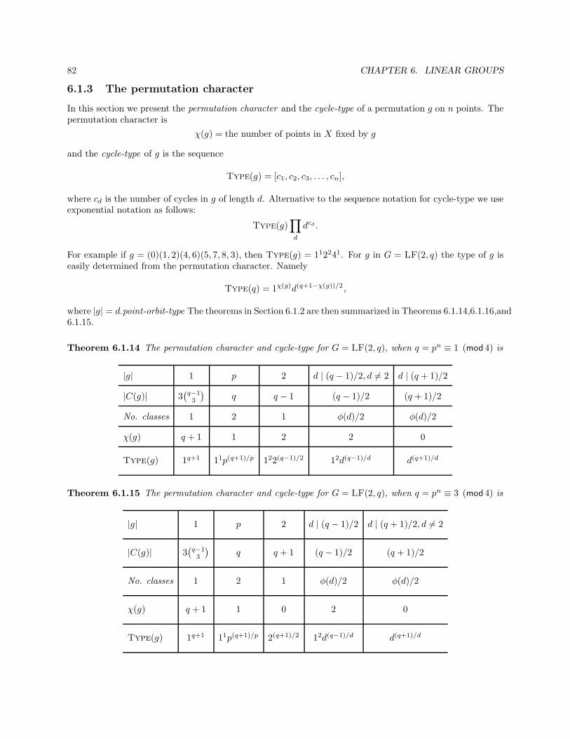
82 CHAPTER 6. LINEAR GROUPS
6.1.3 The permutation character
In this section we present the permutation character and the cycle-type of a permutation g on n points. Thepermutation character is
χ(g) = the number of points in X fixed by g
and the cycle-type of g is the sequence
Type(g) = [c1, c2, c3, . . . , cn],
where cd is the number of cycles in g of length d. Alternative to the sequence notation for cycle-type we useexponential notation as follows:
Type(g)∏
d
dcd .
For example if g = (0)(1, 2)(4, 6)(5, 7, 8, 3), then Type(g) = 112241. For g in G = LF(2, q) the type of g iseasily determined from the permutation character. Namely
Type(q) = 1χ(g)d(q+1−χ(g))/2,
where |g| = d.point-orbit-type The theorems in Section 6.1.2 are then summarized in Theorems 6.1.14,6.1.16,and6.1.15.
Theorem 6.1.14 The permutation character and cycle-type for G = LF(2, q), when q = pn ≡ 1 (mod 4) is
|g| 1 p 2 d | (q − 1)/2, d 6= 2 d | (q + 1)/2
|C(g)| 3(q−13
)q q − 1 (q − 1)/2 (q + 1)/2
No. classes 1 2 1 φ(d)/2 φ(d)/2
χ(g) q + 1 1 2 2 0
Type(g) 1q+1 11p(q+1)/p 122(q−1)/2 12d(q−1)/d d(q+1)/d
Theorem 6.1.15 The permutation character and cycle-type for G = LF(2, q), when q = pn ≡ 3 (mod 4) is
|g| 1 p 2 d | (q − 1)/2 d | (q + 1)/2, d 6= 2
|C(g)| 3(q−13
)q q + 1 (q − 1)/2 (q + 1)/2
No. classes 1 2 1 φ(d)/2 φ(d)/2
χ(g) q + 1 1 0 2 0
Type(g) 1q+1 11p(q+1)/p 2(q+1)/2 12d(q−1)/d d(q+1)/d
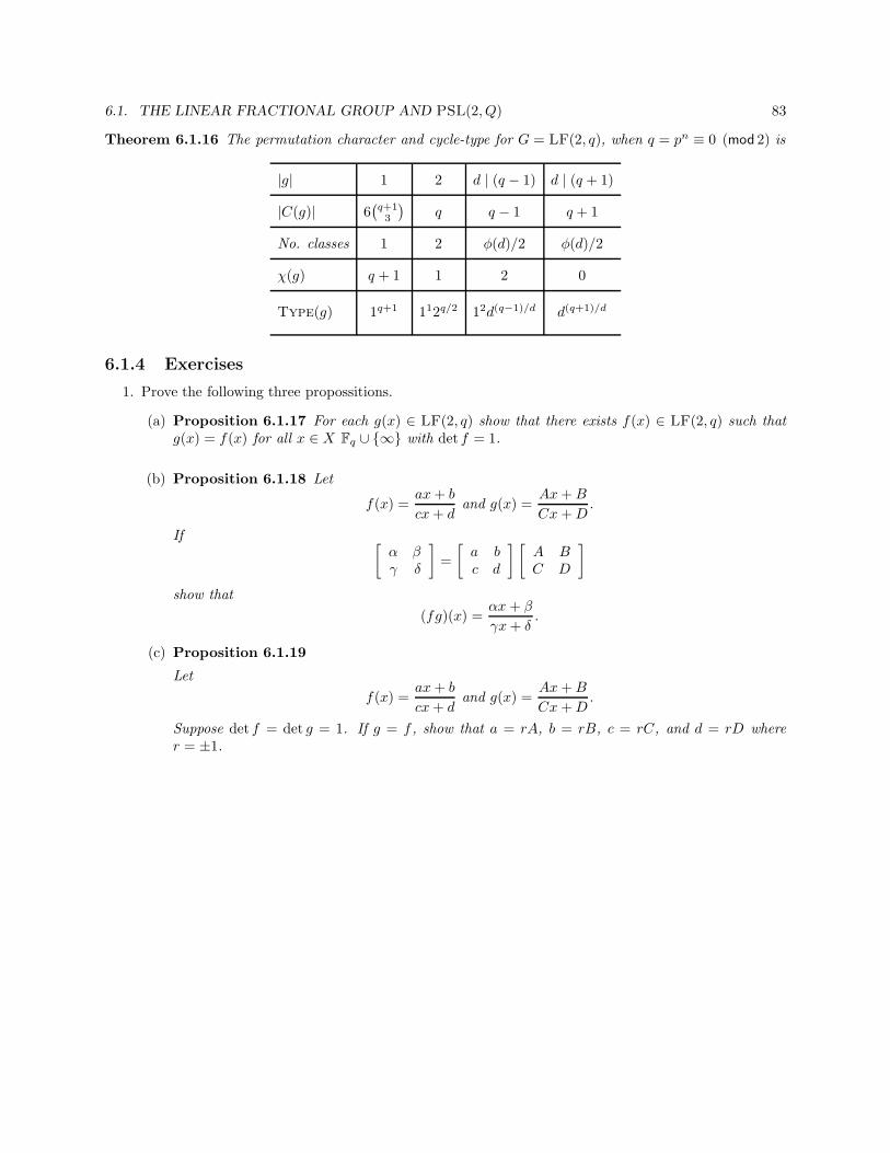
6.1. THE LINEAR FRACTIONAL GROUP AND PSL(2, Q) 83
Theorem 6.1.16 The permutation character and cycle-type for G = LF(2, q), when q = pn ≡ 0 (mod 2) is
|g| 1 2 d | (q − 1) d | (q + 1)
|C(g)| 6(q+13
)q q − 1 q + 1
No. classes 1 2 φ(d)/2 φ(d)/2
χ(g) q + 1 1 2 0
Type(g) 1q+1 112q/2 12d(q−1)/d d(q+1)/d
6.1.4 Exercises
1. Prove the following three propossitions.
(a) Proposition 6.1.17 For each g(x) ∈ LF(2, q) show that there exists f(x) ∈ LF(2, q) such thatg(x) = f(x) for all x ∈ X Fq ∪ ∞ with det f = 1.
(b) Proposition 6.1.18 Let
f(x) =ax+ b
cx+ dand g(x) =
Ax+B
Cx +D.
If [α βγ δ
]
=
[a bc d
] [A BC D
]
show that
(fg)(x) =αx + β
γx+ δ.
(c) Proposition 6.1.19
Let
f(x) =ax+ b
cx+ dand g(x) =
Ax+B
Cx +D.
Suppose det f = det g = 1. If g = f , show that a = rA, b = rB, c = rC, and d = rD wherer = ±1.


![public.gettysburg.edupublic.gettysburg.edu/~franpe02/files/[Baela_Bajnok]_Additive... · Series Editors Miklos Bona Donald L. Kreher Douglas West Patrice Ossona de Mendez Introduction](https://img.pdfslide.us/doc/110x75/5fd20622fccad917db184e30/franpe02filesbaelabajnokadditive-series-editors-miklos-bona-donald-l.jpg)