4700 West 77th Street Minneapolis, MN 55435-4803 Phone: 952.832.2600 Fax: 952.832.2601

Groundwater Modeling of the NorthMet Plant Site

Supporting Document for Water Modeling Data Package Volume 2 – Plant Site

Prepared for Poly Met Mining Inc.

January 2015

P:\Mpls\23 MN\69\2369862\WorkFiles\APA\Support Docs\Water Modeling Package Doc\Attachment\Plant Site\Attachment A - MODFLOW\FEISPlantSiteMODFLOWReport_v1d11.docx

i

Groundwater Modeling of the NorthMet Plant Site

January 2015

ContentsAcronyms and Abbreviations ........................................................................................................................................................... v

1.0 Introduction ........................................................................................................................................................................... 1

1.1 Objectives .......................................................................................................................................................................... 1

1.2 Background ....................................................................................................................................................................... 1

1.3 Report Organization ...................................................................................................................................................... 2

2.0 Conceptual Model ............................................................................................................................................................... 4

2.1 Geologic Units .................................................................................................................................................................. 4

2.1.1 Native Unconsolidated Deposits ......................................................................................................................... 4

2.1.2 Non-Native Deposits ............................................................................................................................................... 6

2.1.3 Bedrock .......................................................................................................................................................................... 7

2.2 Sources and Sinks for Water ...................................................................................................................................... 8

2.3 Local Flow System .......................................................................................................................................................... 8

2.4 Hydrologic Model Selection ....................................................................................................................................... 9

3.0 Model Construction and Calibration ..........................................................................................................................11

3.1 Model Grid and Layers ...............................................................................................................................................11

3.2 Boundary Conditions ...................................................................................................................................................12

3.3 Hydraulic Conductivity and Storage .....................................................................................................................13

3.4 Recharge ..........................................................................................................................................................................13

3.5 Current Conditions Model Calibration .................................................................................................................14

3.5.1 Calibration Objective..............................................................................................................................................15

3.5.2 Calibration Parameters ..........................................................................................................................................15

3.5.3 Calibration Data Sets..............................................................................................................................................16

3.5.4 Regularization and Prior Information ..............................................................................................................18

3.5.5 Calibration Results ..................................................................................................................................................18

3.5.6 Assumptions and Limitations of the Model ..................................................................................................21

4.0 Predictive Simulations ......................................................................................................................................................23

4.1 Modifications to the Current Conditions Model ..............................................................................................24

4.1.1 Model Layers .............................................................................................................................................................24

4.1.2 Boundary Conditions .............................................................................................................................................24

ii

4.1.3 Hydraulic Conductivity ..........................................................................................................................................25

4.1.4 Recharge .....................................................................................................................................................................26

4.2 Predictive Simulation Results ...................................................................................................................................28

4.2.1 Pond Seepage and Discharge to GoldSim Groundwater Flow Paths .................................................28

4.2.2 Particle Tracking Simulations ..............................................................................................................................30

4.2.3 Thickness of Unsaturated Zones .......................................................................................................................31

5.0 Summary and Conclusions .............................................................................................................................................33

6.0 References ............................................................................................................................................................................35

iii

List of Tables

Table 2-1 Hydraulic Conductivity Measured During Single-Well Pumping Tests in Unconsolidated Materials. ............................................................................................................................... 5

Table 2-2 Hydraulic Conductivity Measured in 2014 in Unconsolidated Materials Using Slug Tests.......................................................................................................................................................................... 6

Table 2-3 Hydraulic conductivity measured in bedrock during packer tests. ................................................. 8Table 3-1 Transient Calibration Stress Periods ......................................................................................................... 15Table 3-2 Calibration Statistics for Observations .................................................................................................... 19Table 3-3 Estimated Seepage Rates to GoldSim Groundwater Flow Paths from Current

Conditions Simulation .................................................................................................................................... 20Table 3-4 Flow Calibration Observations and Simulated Values ....................................................................... 21Table 4-1 Pond Elevations Used for Predictive Simulations ................................................................................ 25Table 4-2 Recharge Rates Used for Predictive Simulations ................................................................................. 27Table 4-3 Estimated Seepage Rates From Current Conditions and Predictive Simulations ................... 28Table 4-4 Percentage of FTB Pond Seepage Discharging to Each GoldSim Groundwater Flow

Path ........................................................................................................................................................................ 30Table 4-5 Percentage of FTB Dam Infiltration Discharging to Each GoldSim Groundwater Flow

Path ........................................................................................................................................................................ 31Table 4-6 Estimated Depth of Unsaturated Material in FTB Dams and Beaches ........................................ 31Table 4-7 Estimated Depth of Unsaturated Material below LTVSMC Tailings ............................................. 32

List of Figures

Figure 3-1 Comparison of Modeled and Measured Steady-State and Transient Heads .......................... 19Figure 3-2 Comparison of Modeled and Measured Drawdown at Tailings Basin Piezometers ............. 20Figure 4-1 Summary of Estimated Tailings Basin Flow Rates ............................................................................... 29

List of Large Tables

Large Table 1 Calibration Parameters, Parameter Bounds, and Optimized ValuesLarge Table 2 Steady-State Calibration Observations and Simulated ValuesLarge Table 3 Transient Head Calibration Observations and Simulated ValuesLarge Table 4 Transient Drawdown Calibration Observations and Simulated ValuesLarge Table 5 Hydraulic Conductivity Values Used for Flotation Tailings in Predictive SimulationsLarge Table 6 Beach Seepage Directions by Percent of Flow to Each Flow Path

iv

List of Large Figures

Large Figure 1 Site LayoutLarge Figure 2 NorthMet Bulk Tailings 2005 Permeability Test ResultsLarge Figure 3 Model Domain and GridLarge Figure 4 Layer 2 ThicknessLarge Figure 5 Model Boundary Conditions Layers 1 and 2Large Figure 6 Hydraulic Conductivity Zones in Layer 1Large Figure 7 Hydraulic Conductivity Zones in Layer 2Large Figure 8 Recharge Zone Extents First Active LayerLarge Figure 9 Calibration Observation LocationsLarge Figure 10 Simulated Groundwater Head Contours and Head Residuals in Layer 1Large Figure 11 Simulated Groundwater Head Contours and Head Residuals in Layer 2Large Figure 12 Observed vs Simulated Drawdown: DH96-28, DH96-30, DH96-32, DH96-37Large Figure 13 Observed vs Simulated Drawdown: PN1J-99, F-2, P2HA-99, P2HB-99Large Figure 14 Observed vs Simulated Drawdown: P1H1-99, P1H-99, P3H1-99, P2H1-99Large Figure 15 Observed vs Simulated Drawdown: P3H-99, DNR-1, DNR-2, DNR-3Large Figure 16 Observed vs Simulated Drawdown: DNR-4, DNR-5, DNR-6, GW004Large Figure 17 Observed vs Simulated Drawdown: GW005, A-1, A-3, A-9Large Figure 18 Observed vs Simulated Drawdown: B-2, D-1, D-4, G-2Large Figure 19 Flotation Tailings Basin Configuration - Mine Year 1Large Figure 20 Flotation Tailings Basin Configuration - Mine Year 7Large Figure 21 Flotation Tailings Basin Configuration - Mine Year 8Large Figure 22 Flotation Tailings Basin Configuration - Mine Year 18 and 20 Long-term ClosureLarge Figure 23 Mine Year 1 Boundary Conditions - Layer 1Large Figure 24 Mine Year 7 Boundary Conditions - Layer 1Large Figure 25 Mine Year 8 Boundary Conditions - Layer 1Large Figure 26 Long-term Closure Boundary Conditions - Layer 1Large Figure 27 Bottom Layer Boundary Conditions - Predictive SimulationsLarge Figure 28 Fate and Transport of Infiltration - Current ConditionsLarge Figure 29 Fate and Transport of Tailings Basin Infiltration - Mine Year 1Large Figure 30 Fate and Transport of Tailings Basin Infiltration - Mine Year 7Large Figure 31 Fate and Transport of Tailings Basin Infiltration - Mine Year 8Large Figure 32 Fate and Transport of Tailings Basin Infiltration - Mine Year 18Large Figure 33 Fate and Transport of Tailings Basin Infiltration - Mine Year 20Large Figure 34 Fate and Transport of Tailings Basin Infiltration - Long-term Closure

v

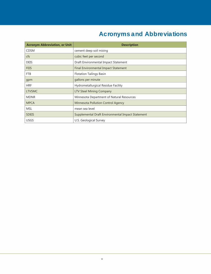
Acronyms and Abbreviations Acronym Abbreviation, or Unit Description

CDSM cement deep soil mixing

cfs cubic feet per second

DEIS Draft Environmental Impact Statement

FEIS Final Environmental Impact Statement

FTB Flotation Tailings Basin

gpm gallons per minute

HRF Hydrometallurgical Residue Facility

LTVSMC LTV Steel Mining Company

MDNR Minnesota Department of Natural Resources

MPCA Minnesota Pollution Control Agency

MSL mean sea level

SDEIS Supplemental Draft Environmental Impact Statement

USGS U.S. Geological Survey

1

1.0 IntroductionThis report describes the technical approach, rationale, and scope for groundwater flow modeling that was conducted for the Poly Met Mining Inc. (PolyMet) NorthMet Project (Project) Plant Site. The groundwater modeling was completed to support the probabilistic modeling used to estimate Project water balances and water quality impacts presented in the NorthMet Project Water Modeling Data Package Volume 2 – Plant Site (Reference (1)). This report describes the objectives of the groundwater modeling, the site conceptual model, the modeling methodology, and the modeling results. The modeling was based on the current understanding of the Plant Site conditions and the project description (Reference (2)) developed for the Final Environmental Impact Statement (FEIS).

In this report, the Flotation Tailings Basin (FTB) is the newly constructed Flotation Tailings impoundment and the Tailings Basin is the existing LTV Steel Mining Company (LTVSMC) Tailings Basin as well as the combined LTVSMC Tailings Basin and the FTB.

1.1 ObjectivesThe primary objectives for the Plant Site groundwater flow modeling were to:

estimate the seepage loss from the LTVSMC Tailings Basin ponds under current conditions and the FTB pond(s) during operations and long-term closure

estimate the average annual infiltration rate throughout the Tailings Basin under current conditions

estimate the discharge rate of seepage entering each of the five groundwater flow paths represented in the GoldSim model (Reference (1), Reference (3) during current conditions, operations and long-term closure

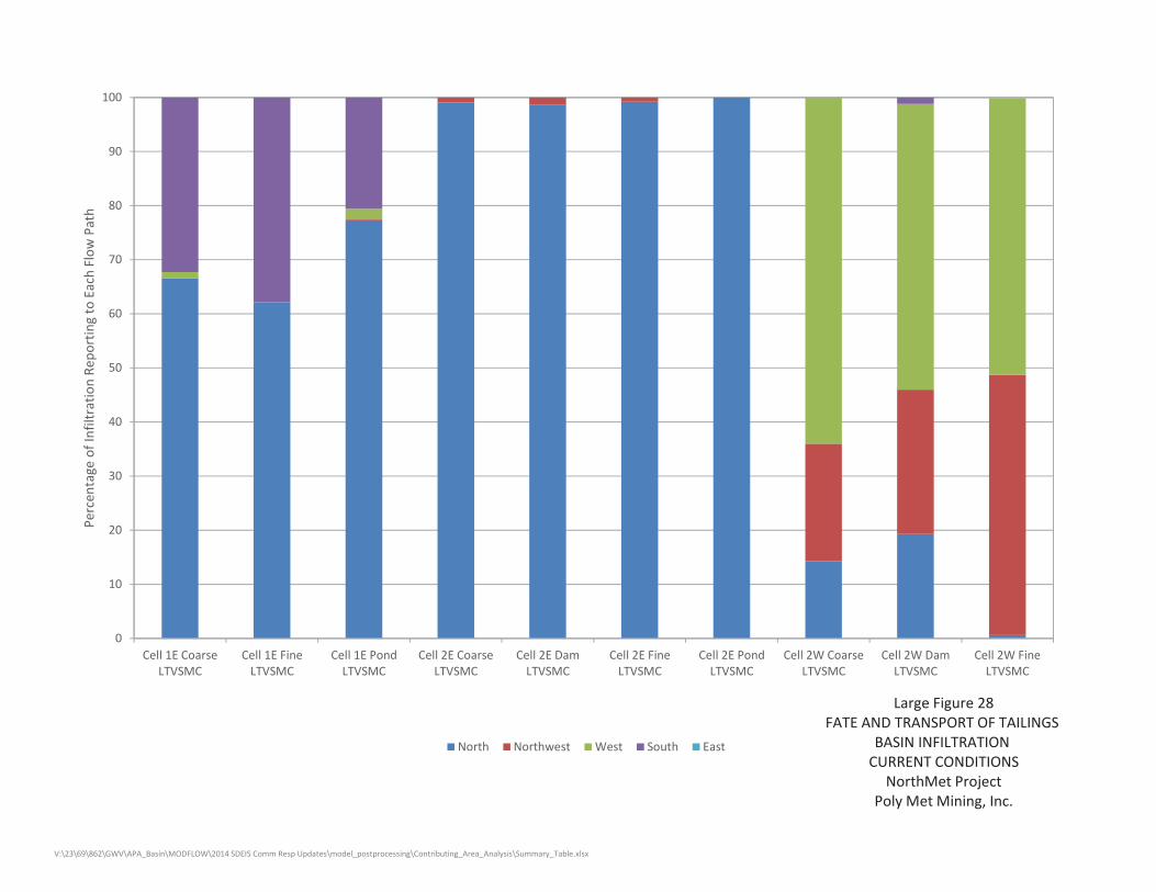
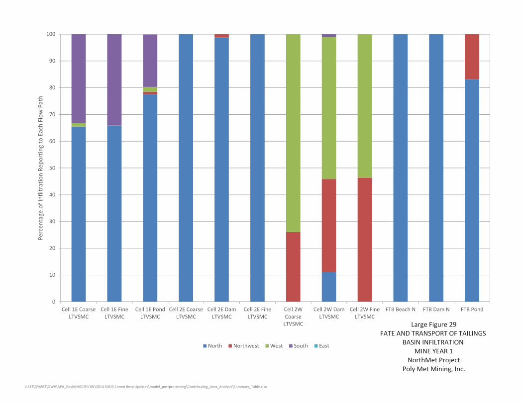
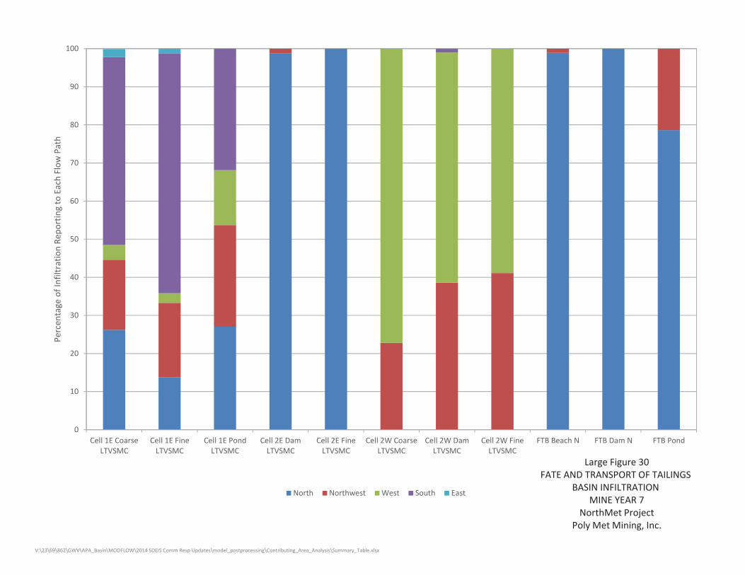
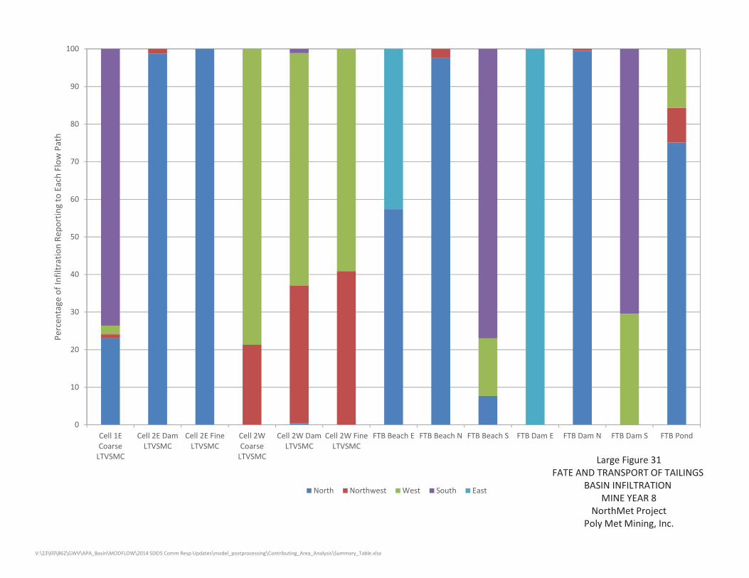
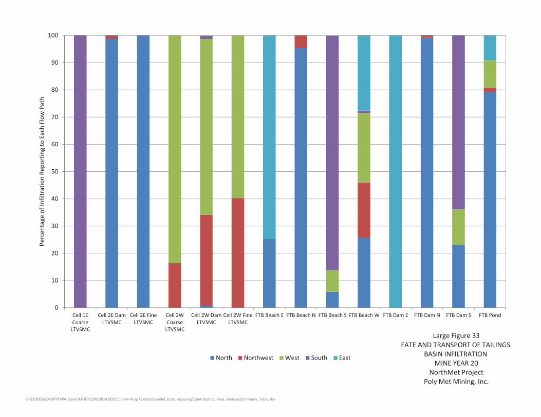
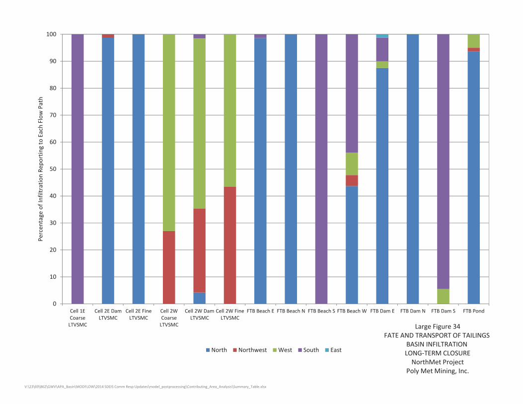
estimate what proportion of the water that infiltrates the various material types present at the surface of the Tailings Basin ultimately reports to each of the GoldSim groundwater flow paths

estimate the depth of the phreatic surface within each of the material types present at the surface of the Tailings Basin

A series of groundwater models were developed to meet these objectives. These models were designed to simulate current conditions, conditions during operations, and conditions during long-term closure.

1.2 BackgroundThe Tailings Basin, covering an area of approximately 2,600 acres (about 4 square miles), was previously used by LTVSMC and its predecessor Erie Mining Company for disposal of taconite tailings. The facility is unlined and was constructed in stages beginning in the 1950’s. Taconite tailings were deposited from 1957 to January of 2001, when the Tailings Basin was shut down. It has been inactive since then except for reclamation activities consistent with the Minnesota Department of Natural Resources (MDNR) approved

2

closure plan currently managed by Cliffs Erie, and more recently, activities associated with the April 6, 2010, Consent Decree between Cliffs Erie and the Minnesota Pollution Control Agency (MPCA).There are three discrete cells in the LTVSMC Tailings Basin, Cells 1E, 2E, and 2W, as shown on Large Figure 1. Cell 2W is the largest (1,447 acres) and has the highest elevation of the three cells, with an average fill height of 200 feet (approximately 1,725 feet mean sea level (MSL)). Cell 2W is currently the driest of the cells and has gradually lost the ponded water that remained following taconite processing. Cell 1E is approximately 980 acres and rises approximately 125 feet above the surrounding ground level (approximately 1,650 feet MSL); Cell 2E is about 620 acres and has the lowest elevation of all of the existing cells, rising approximately 60 feet above surrounding ground level (approximately 1,555 feet). Cells 1E and 2E currently contain ponded water. The existing Tailings Basin does not have an overflow or discharge structure.

Ore processing associated with the Project will produce two types of mineral waste: Hydrometallurgical Residue and Flotation Tailings. These two wastes will be disposed of in separate facilities. Hydrometallurgical Residue will be stored in the Hydrometallurgical Residue Facility (HRF), a lined basin constructed on top of the Emergency Basin located near the southwestern corner of the Tailings Basin (Reference (4)). The FTB will be constructed in stages atop existing Cells 1E and 2E of the Tailings Basin for disposal of Flotation Tailings. FTB staging and sequencing is described in Reference (5). The FTB design includes seepage capture systems (the FTB Containment System and the FTB South Seepage Management System), as described in Reference (6).

During the Draft Environmental Impact Statement (DEIS) process, a series of numerical groundwater flow models were developed for the Tailings Basin (Attachment A-6 of Reference (7), Attachment A-6 of Reference (7)). The DEIS versions of the model calibrations were steady-state and did not simulate changes in water levels within the basin. However, after LTVSMC operations and deposition of tailings ceased in 2001, the groundwater mound beneath the Tailings Basin began to dissipate, and the quantity of seepage leaving the Tailings Basin area has decreased. As part of the modeling effort for the Supplemental Draft Environmental Impact Statement (SDEIS), the calibration of the groundwater model was updated to represent transient conditions following LTVSMC closure until present, and to simulate the observed dissipation of the groundwater mound beneath the basin. For the FEIS modeling effort, the groundwater models were updated to incorporate groundwater elevation data collected through 2013 and changes as recommended by the Co-lead Agencies. This report documents the current version of the models developed for the FEIS.

FTB seepage capture systems were not simulated using the models described in this report. Additional groundwater modeling was conducted to support the design of the FTB Containment System. That modeling used results from the groundwater flow modeling described in this report and is described under separate cover in Attachment C of Reference (6).

1.3 Report Organization This report is organized into five sections, including this introduction. Section 2.0 presents the conceptual model of hydrogeology at the Plant Site. Section 3.0 discusses the modeling approach and calibration

3

methods and results. Predictive simulations of operations and long-term closure conditions are presented in Section 4.0. A report summary and conclusions are presented in Section 5.0.

4

2.0 Conceptual Model A hydrogeologic conceptual model is a schematic description of how water enters, flows through, and leaves the groundwater system. Its purpose is to describe the major sources and sinks of water, the grouping or division of hydrostratigraphic units into aquifers and aquitards, the direction of groundwater flow, the interflow of groundwater between aquifers, and the interflow of water between surface waters and groundwater. The hydrogeologic conceptual model is both scale-dependent (e.g., local conditions may not be identical to regional conditions) and dependent upon the objectives. It is important when developing a conceptual model to strive for an effective balance: the model should be kept as simple as possible while still adequately representing the system to analyze the objectives at hand.

2.1 Geologic Units This section provides an overview of the Plant Site geology and the hydraulic properties of each geologic unit, particularly as they pertain to the development of the groundwater flow models. A more detailed summary of the current understanding of bedrock structure and hydrogeology at the Mine Site and the Plant Site, and description of the regional and local bedrock geology and hydrogeology, including the nature of fractured bedrock, can be found in Reference (8).

2.1.1 Native Unconsolidated Deposits The native unconsolidated deposits in the vicinity of Plant Site are a relatively thin mantle of Quaternary-age glacial till and associated reworked sediments, most of which were deposited and reworked by the retreating Rainy Lobe during the last glacial period in association with the development of the Vermillion moraine complex (Reference (9))). Near the Tailings Basin, unconsolidated deposits have been characterized based on soil borings and monitoring wells, which have been completed to the north and west of the Tailings Basin. The unconsolidated deposits generally consist of discontinuous lenses of silty sand to poorly graded sand with silt, to poorly graded sand with gravel. Very little silt or clay has been encountered, with the exception of the soil boring drilled near monitoring well GW006, where several feet of silt is interbedded with silty sand (Reference (10)). In places, the till is overlain by organic peat deposits. Depth to bedrock in the area surrounding the Tailings Basin is generally less than 50 feet. The unconsolidated deposits generally thicken in a northerly direction toward the Embarrass River. Wetland areas also become more common to the north, off the northern flank of the Giant’s Range, the granite outcrops located adjacent to the Tailings Basin. These wetland areas are underlain by thin glacial drift and lacustrine deposits, which were deposited by the retreating Rainy Lobe and associated lakes that were trapped between the retreating ice margin and the Giant’s Range.

Siegel and Ericson (Reference (11)) indicate that the till of the Rainy Lobe has an estimated hydraulic conductivity range of 0.1 to 30 feet/day. In-situ pumping tests were conducted at monitoring wells GW001, GW006, GW007, GW009, GW010, GW011, and GW012 to estimate hydraulic conductivity, as described in detail in Attachment F of Reference (12). The data collected during the tests was used to estimate the hydraulic conductivity of the unconsolidated deposits using three different methods; the Moench solution (Reference (13)), the Theis solution (Reference (14)), and using specific capacity data (Reference (15)). The hydraulic conductivity estimates from each solution are different at each location.

5

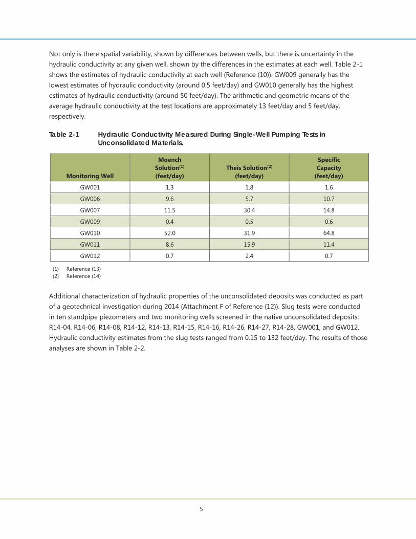
Not only is there spatial variability, shown by differences between wells, but there is uncertainty in the hydraulic conductivity at any given well, shown by the differences in the estimates at each well. Table 2-1 shows the estimates of hydraulic conductivity at each well (Reference (10)). GW009 generally has the lowest estimates of hydraulic conductivity (around 0.5 feet/day) and GW010 generally has the highest estimates of hydraulic conductivity (around 50 feet/day). The arithmetic and geometric means of the average hydraulic conductivity at the test locations are approximately 13 feet/day and 5 feet/day, respectively.

Table 2-1 Hydraulic Conductivity Measured During Single-Well Pumping Tests in Unconsolidated Materials.

Monitoring Well

Moench Solution(1) (feet/day)

Theis Solution(2) (feet/day)

Specific Capacity

(feet/day)

GW001 1.3 1.8 1.6

GW006 9.6 5.7 10.7

GW007 11.5 30.4 14.8

GW009 0.4 0.5 0.6

GW010 52.0 31.9 64.8

GW011 8.6 15.9 11.4

GW012 0.7 2.4 0.7

(1) Reference (13) (2) Reference (14)

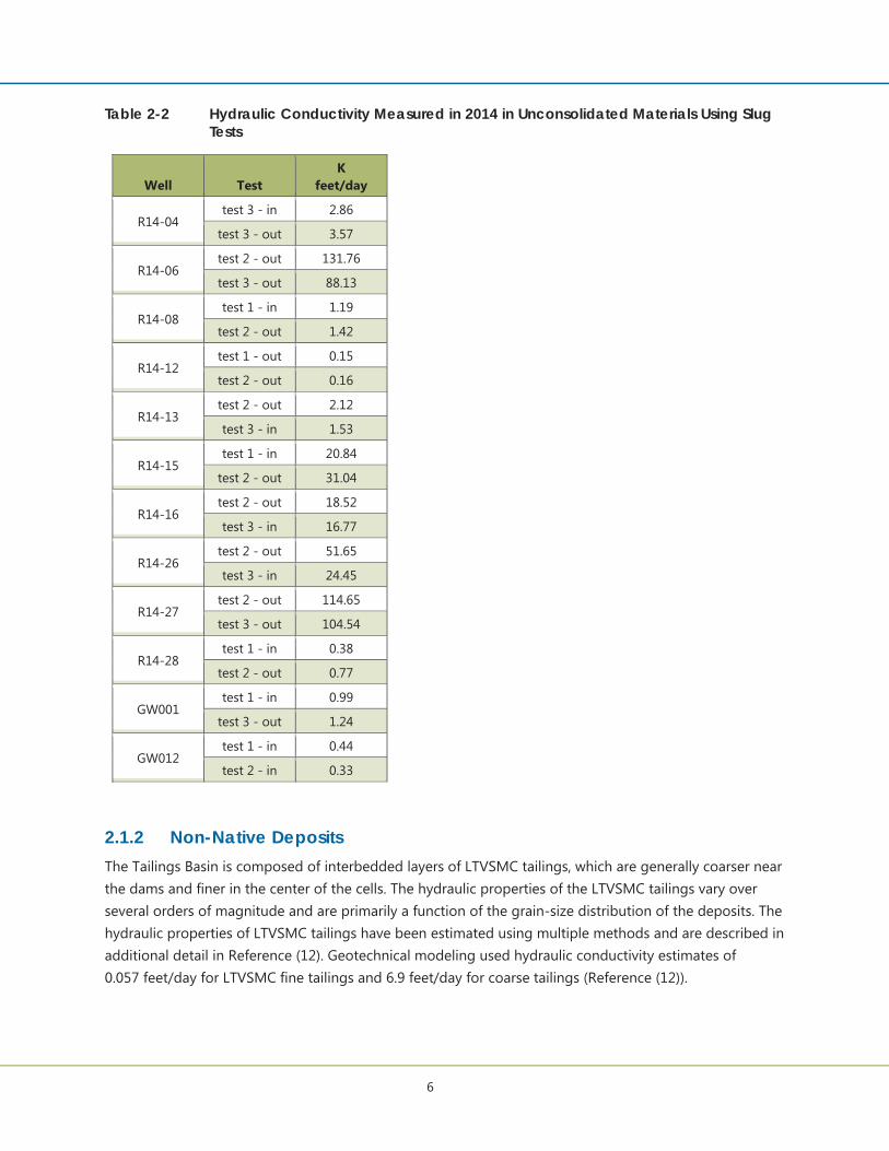
Additional characterization of hydraulic properties of the unconsolidated deposits was conducted as part of a geotechnical investigation during 2014 (Attachment F of Reference (12)). Slug tests were conducted in ten standpipe piezometers and two monitoring wells screened in the native unconsolidated deposits: R14-04, R14-06, R14-08, R14-12, R14-13, R14-15, R14-16, R14-26, R14-27, R14-28, GW001, and GW012. Hydraulic conductivity estimates from the slug tests ranged from 0.15 to 132 feet/day. The results of those analyses are shown in Table 2-2.

6

Table 2-2 Hydraulic Conductivity Measured in 2014 in Unconsolidated Materials Using Slug Tests

Well Test K

feet/day

R14-04 test 3 - in 2.86

test 3 - out 3.57

R14-06 test 2 - out 131.76

test 3 - out 88.13

R14-08 test 1 - in 1.19

test 2 - out 1.42

R14-12 test 1 - out 0.15

test 2 - out 0.16

R14-13 test 2 - out 2.12

test 3 - in 1.53

R14-15 test 1 - in 20.84

test 2 - out 31.04

R14-16 test 2 - out 18.52

test 3 - in 16.77

R14-26 test 2 - out 51.65

test 3 - in 24.45

R14-27 test 2 - out 114.65

test 3 - out 104.54

R14-28 test 1 - in 0.38

test 2 - out 0.77

GW001 test 1 - in 0.99

test 3 - out 1.24

GW012 test 1 - in 0.44

test 2 - in 0.33

2.1.2 Non-Native Deposits The Tailings Basin is composed of interbedded layers of LTVSMC tailings, which are generally coarser near the dams and finer in the center of the cells. The hydraulic properties of the LTVSMC tailings vary over several orders of magnitude and are primarily a function of the grain-size distribution of the deposits. The hydraulic properties of LTVSMC tailings have been estimated using multiple methods and are described in additional detail in Reference (12). Geotechnical modeling used hydraulic conductivity estimates of 0.057 feet/day for LTVSMC fine tailings and 6.9 feet/day for coarse tailings (Reference (12)).

7

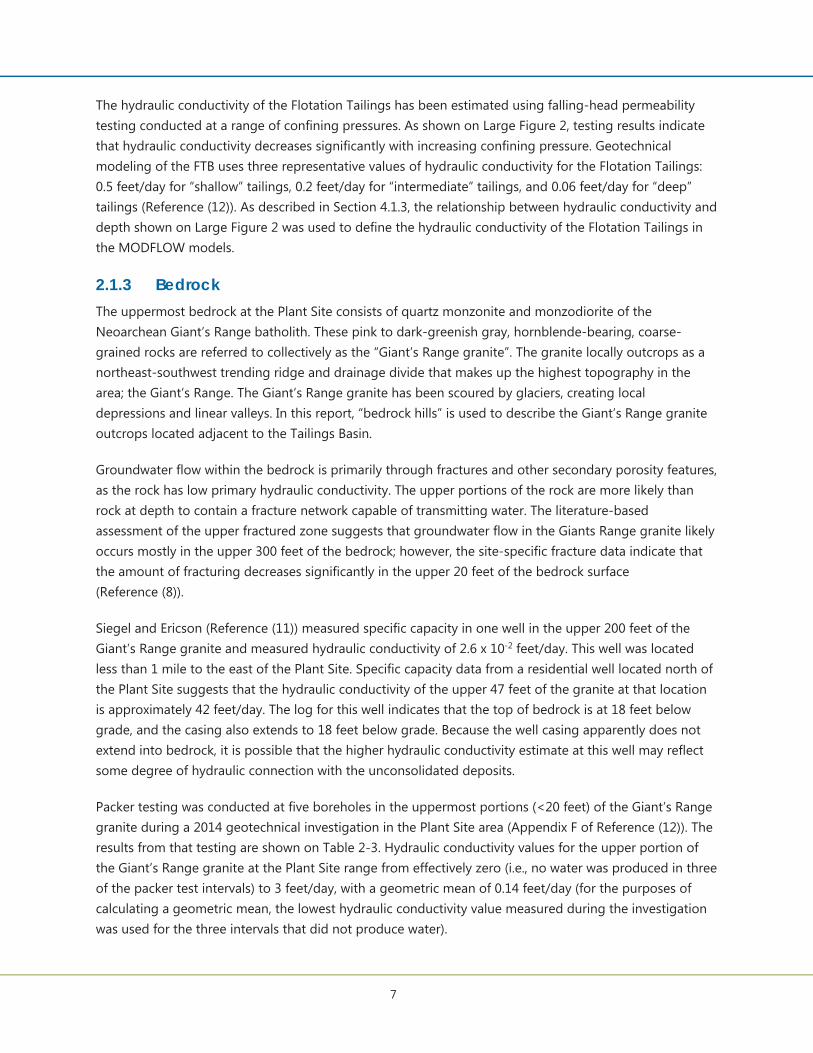
The hydraulic conductivity of the Flotation Tailings has been estimated using falling-head permeability testing conducted at a range of confining pressures. As shown on Large Figure 2, testing results indicate that hydraulic conductivity decreases significantly with increasing confining pressure. Geotechnical modeling of the FTB uses three representative values of hydraulic conductivity for the Flotation Tailings: 0.5 feet/day for “shallow” tailings, 0.2 feet/day for “intermediate” tailings, and 0.06 feet/day for “deep” tailings (Reference (12)). As described in Section 4.1.3, the relationship between hydraulic conductivity and depth shown on Large Figure 2 was used to define the hydraulic conductivity of the Flotation Tailings in the MODFLOW models.

2.1.3 BedrockThe uppermost bedrock at the Plant Site consists of quartz monzonite and monzodiorite of the Neoarchean Giant’s Range batholith. These pink to dark-greenish gray, hornblende-bearing, coarse-grained rocks are referred to collectively as the “Giant’s Range granite”. The granite locally outcrops as a northeast-southwest trending ridge and drainage divide that makes up the highest topography in the area; the Giant’s Range. The Giant’s Range granite has been scoured by glaciers, creating local depressions and linear valleys. In this report, “bedrock hills” is used to describe the Giant’s Range granite outcrops located adjacent to the Tailings Basin.

Groundwater flow within the bedrock is primarily through fractures and other secondary porosity features, as the rock has low primary hydraulic conductivity. The upper portions of the rock are more likely than rock at depth to contain a fracture network capable of transmitting water. The literature-based assessment of the upper fractured zone suggests that groundwater flow in the Giants Range granite likely occurs mostly in the upper 300 feet of the bedrock; however, the site-specific fracture data indicate that the amount of fracturing decreases significantly in the upper 20 feet of the bedrock surface (Reference (8)).

Siegel and Ericson (Reference (11)) measured specific capacity in one well in the upper 200 feet of the Giant’s Range granite and measured hydraulic conductivity of 2.6 x 10-2 feet/day. This well was located less than 1 mile to the east of the Plant Site. Specific capacity data from a residential well located north of the Plant Site suggests that the hydraulic conductivity of the upper 47 feet of the granite at that location is approximately 42 feet/day. The log for this well indicates that the top of bedrock is at 18 feet below grade, and the casing also extends to 18 feet below grade. Because the well casing apparently does not extend into bedrock, it is possible that the higher hydraulic conductivity estimate at this well may reflect some degree of hydraulic connection with the unconsolidated deposits.

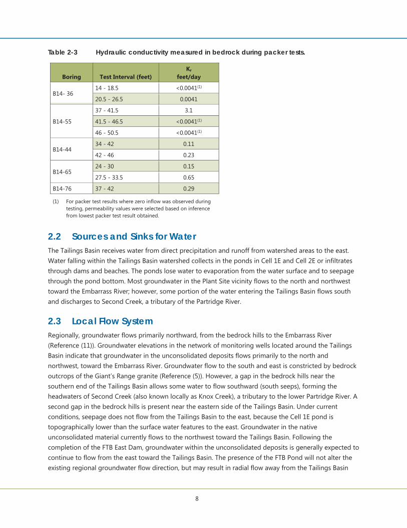
Packer testing was conducted at five boreholes in the uppermost portions (<20 feet) of the Giant’s Range granite during a 2014 geotechnical investigation in the Plant Site area (Appendix F of Reference (12)). The results from that testing are shown on Table 2-3. Hydraulic conductivity values for the upper portion of the Giant’s Range granite at the Plant Site range from effectively zero (i.e., no water was produced in three of the packer test intervals) to 3 feet/day, with a geometric mean of 0.14 feet/day (for the purposes of calculating a geometric mean, the lowest hydraulic conductivity value measured during the investigation was used for the three intervals that did not produce water).

8

Table 2-3 Hydraulic conductivity measured in bedrock during packer tests.

Boring Test Interval (feet) Kr

feet/day

B14- 36 14 - 18.5 <0.0041(1)

20.5 - 26.5 0.0041

B14-55

37 - 41.5 3.1

41.5 - 46.5 <0.0041(1)

46 - 50.5 <0.0041(1)

B14-44 34 - 42 0.11

42 - 46 0.23

B14-65 24 - 30 0.15

27.5 - 33.5 0.65

B14-76 37 - 42 0.29

(1) For packer test results where zero inflow was observed during testing, permeability values were selected based on inference from lowest packer test result obtained.

2.2 Sources and Sinks for Water The Tailings Basin receives water from direct precipitation and runoff from watershed areas to the east. Water falling within the Tailings Basin watershed collects in the ponds in Cell 1E and Cell 2E or infiltrates through dams and beaches. The ponds lose water to evaporation from the water surface and to seepage through the pond bottom. Most groundwater in the Plant Site vicinity flows to the north and northwest toward the Embarrass River; however, some portion of the water entering the Tailings Basin flows south and discharges to Second Creek, a tributary of the Partridge River.

2.3 Local Flow System Regionally, groundwater flows primarily northward, from the bedrock hills to the Embarrass River (Reference (11)). Groundwater elevations in the network of monitoring wells located around the Tailings Basin indicate that groundwater in the unconsolidated deposits flows primarily to the north and northwest, toward the Embarrass River. Groundwater flow to the south and east is constricted by bedrock outcrops of the Giant’s Range granite (Reference (5)). However, a gap in the bedrock hills near the southern end of the Tailings Basin allows some water to flow southward (south seeps), forming the headwaters of Second Creek (also known locally as Knox Creek), a tributary to the lower Partridge River. A second gap in the bedrock hills is present near the eastern side of the Tailings Basin. Under current conditions, seepage does not flow from the Tailings Basin to the east, because the Cell 1E pond is topographically lower than the surface water features to the east. Groundwater in the native unconsolidated material currently flows to the northwest toward the Tailings Basin. Following the completion of the FTB East Dam, groundwater within the unconsolidated deposits is generally expected to continue to flow from the east toward the Tailings Basin. The presence of the FTB Pond will not alter the existing regional groundwater flow direction, but may result in radial flow away from the Tailings Basin

9

area on a local scale. Some water could seep through the unconsolidated material below the East Dam. Based on topography and the inferred groundwater divides to the area east of the Tailings Basin, this seepage would likely discharge near the toe of the East Dam, and it is not anticipated to flow east toward the Area 5NW pit or Spring Mine Lake (Reference (16)). As part of the Project, a seepage containment system will be constructed in this area to capture any seepage that would discharge in this area (Reference (6)).

As the Tailings Basin was built up over time, a groundwater mound formed beneath the basin due to seepage from the basin ponds, altering local flow directions and rates. Therefore, the Tailings Basin determines patterns of runoff and infiltration at the Plant Site. Under current conditions, water that infiltrates through the Tailings Basin (from precipitation and seepage from the existing ponds) seeps downward to the native unconsolidated deposits.

Beneath the unconsolidated deposits, low-permeability crystalline bedrock impedes further downward groundwater flow; based on the contrast in hydraulic conductivity between the unconsolidated deposits and bedrock described above, groundwater flow through the bedrock is likely negligible relative to flow through the unconsolidated deposits. Because the unconsolidated deposits are thin and have relatively low hydraulic conductivity, and because the water table is close to the ground surface (which effectively limits the hydraulic gradient), the unconsolidated deposits have a limited capacity to transport Tailings Basin seepage. Therefore, a large portion of that seepage discharges to wetland areas near the Tailings Basin dams, while a small portion remains in the unconsolidated deposits and flows away from the basin laterally as groundwater.

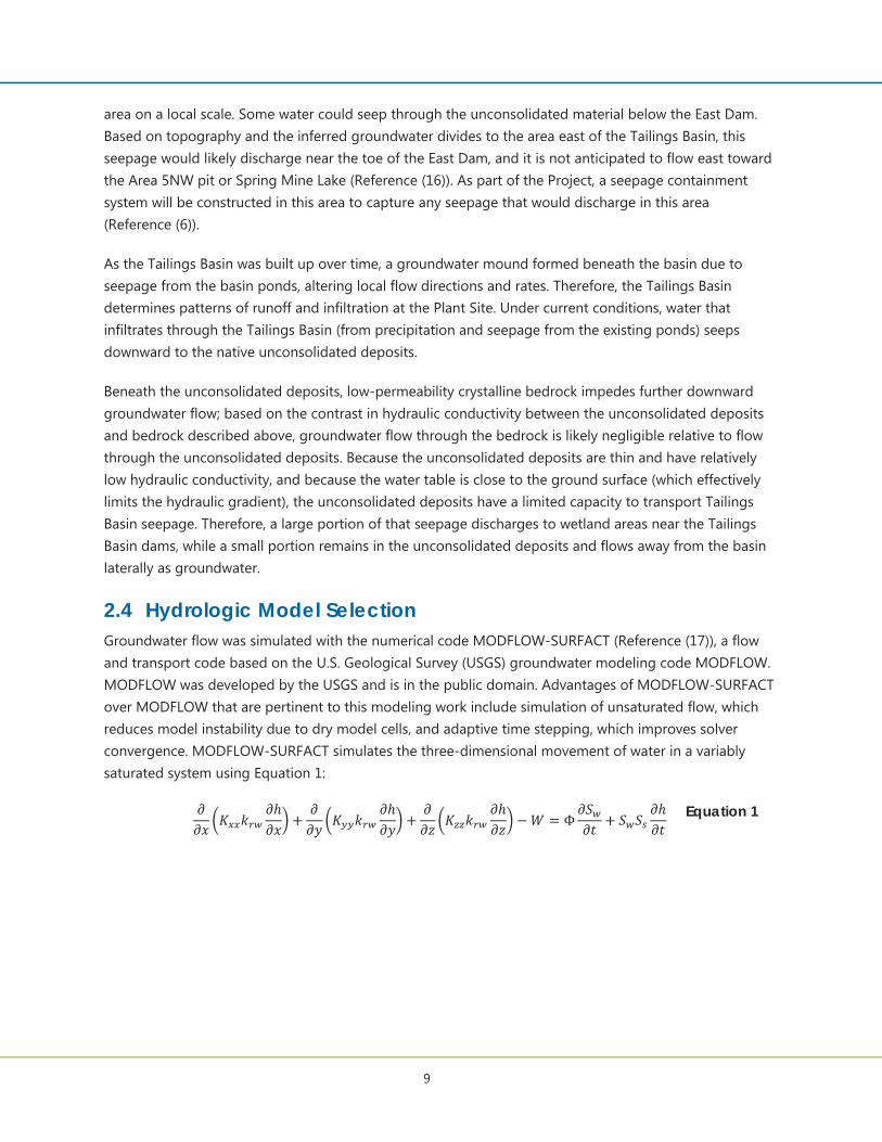
2.4 Hydrologic Model Selection Groundwater flow was simulated with the numerical code MODFLOW-SURFACT (Reference (17)), a flow and transport code based on the U.S. Geological Survey (USGS) groundwater modeling code MODFLOW. MODFLOW was developed by the USGS and is in the public domain. Advantages of MODFLOW-SURFACT over MODFLOW that are pertinent to this modeling work include simulation of unsaturated flow, which reduces model instability due to dry model cells, and adaptive time stepping, which improves solver convergence. MODFLOW-SURFACT simulates the three-dimensional movement of water in a variably saturated system using Equation 1:

Equation 1

10

Where:

x, y, and z are Cartesian coordinates (L) Kxx, Kyy, and Kzz are the principal components of hydraulic conductivity along the x, y, and z axes, respectively (LT-1) krw is the relative permeability, which is a function of water saturation h is the hydraulic head (L) W is a volumetric flux per unit volume and represents source and/or sinks of water (T-1)

is the drainable porosity taken to be equal to the specific yield, Sy Sw is the degree of saturation of water, which is a function of the pressure head Ss is the specific storage of the porous material (L-1) t is time (T)

Pseudo-soil relations were used to define the relative permeability (krw) and the degree of saturation (Sw). It is not necessary to explicitly include information on soil water retention to use pseudo-soil relations.

The particle-tracking code MODPATH (Reference (18)) was used in the predictive simulations. MODPATH uses output files from MODFLOW simulations to compute three-dimensional flow paths by tracking particles throughout the model domain until they reach a boundary, enter an internal source or sink, or are terminated in a process specified by the modeler. MODPATH also tracks the time-of-travel for simulated particles as they move though the model domain.

The graphical user interface Groundwater Vistas (Versions 6) (Reference (19)) was used to support the development of the MODFLOW models, although some elements of the models were developed outside of Groundwater Vistas.

11

3.0 Model Construction and Calibration The conceptual model of the Tailings Basin hydrogeology outlined in Section 2.0 was used to develop a series of numerical simulations for this study. A simulation of conditions since LTVSMC operations ceased in 2001 through December 2013 was used to calibrate model parameters. This simulation is referred to as the “current conditions model” in the discussion that follows. Separate predictive simulations (i.e., forward simulations) were developed for various stages of operations and for long-term closure conditions.

3.1 Model Grid and Layers The active area of the finite-difference grid covers approximately 18 square miles (Large Figure 3), extending from the Embarrass River in the north and west, to the south and east of the former LTVSMC mine pits. The model area is sufficiently large that the model boundaries do not meaningfully affect the model results at the Tailings Basin (Attachment A-6 of Reference (20)). The model grid was refined in the area of interest, with the final grid coarser at the boundaries and outside of the area of interest (cells of approximately 820 feet on a side) and more refined at the Tailings Basin (cells of approximately 100 to 200 feet on a side).

The current conditions models have two layers. Layer 1 is modeled as unconfined and represents the LTVSMC tailings. Layer 2 is modeled as confined and represents the native unconsolidated deposits (glacial drift and peat) and the bedrock hills adjacent to the Tailings Basin. The portions of Layer 1 outside of the footprint of the Tailings Basin were inactivated (i.e., converted to no-flow cells). The bedrock was assumed to have a significantly lower value of hydraulic conductivity than the native unconsolidated deposits and, as such, was treated as a no-flow boundary. The exception to this was in the area of the bedrock hills, where the water table is likely located within the bedrock. In this area, the bottom of Layer 2 was lowered, and the bedrock was simulated as a zone of low hydraulic conductivity. This was necessary to prevent dry cells in Layer 2.

The top elevation for Layer 1 is flat and set at an elevation of 1968.5 feet MSL (or 600 meters, an even increment in metric units, the standard units used to develop the models), which is above the highest elevation in the active model domain. Because Layer 1 is defined as unconfined, the water levels calculated by the model (rather than the top of Layer 1) are used to calculate transmissivity, so the elevation of the top of Layer 1 has no bearing on the simulation results. The bottom elevation for Layer 1 (equal to the top of Layer 2) was defined as the pre-mining topography, using topographic information from the USGS (Reference (21), Reference (22), Reference (23), Reference (24)). The bottom elevation for Layer 2 was defined as the top of bedrock. Bedrock elevations were calculated using a combined bedrock data set, derived from a regional, 30-meter resolution MGS bedrock surface (Reference (25)), into which local bedrock data were incorporated. Groundwater wells and borings completed in the vicinity of the Tailings Basin, at which estimated bedrock elevations were available, were buffered a distance of 3,280.8 feet (or, 1,000 meters, an even increment in metric units, the standard units used to develop the models). The area within the buffer was then clipped from the MGS bedrock surface. Finally, the coordinates of each well, its associated bedrock elevation, and the remaining regional grid data were provided as input to a new surface interpolation. The resulting surface matches the regional grid outside

12

the 3,280.8-feet buffer and within, smoothly transitions to match the field-measured site data. In areas where top of bedrock elevations were above 1,587 feet MSL, (which occurred in bedrock outcrop areas), the bottom of Layer 2 was assigned an elevation of 1,587 feet MSL. In addition, the bottom of Layer 2 was lowered in some areas of the model so that cells in Layer 2 had a minimum thickness of 16.4 feet. The thickness of Layer 2 is presented in Large Figure 4.

3.2 Boundary Conditions Boundary conditions were used to represent surface-water features within the model domain (Large Figure 5). Streams and rivers were simulated as specified-head boundaries in Layer 2 with elevations obtained from USGS 7.5’ quadrangle maps (Reference (21), Reference (22), Reference (23), Reference (24)). The ponds in Cells 1E and 2E were simulated as specified-head boundaries in Layer 1, using water levels reported in the East Range Hydrology Study (Reference (26)) for the current conditions simulation and FTB design elevations for the future conditions simulations. The Cell 1E pond elevation was set at 1,653 feet MSL and Cell 2E pond elevation was set at 1,560 feet MSL for part of the current conditions simulation and allowed to vary between stress periods as calibration parameters for the remainder of the simulation (see Section 3.5 for calibration details). The allowed range of elevations was within the observed elevation range for each pond (Reference (26)).

The River Package in MODFLOW was used to simulate the wetlands surrounding the Tailings Basin as head-dependent flux boundaries. River cells allow water to flow into and out of the boundary, with the flux dependent on a user-specified conductance and the head gradient between the boundary (a constant, user-specified stage) and the aquifer. The extent of wetlands areas was set based on delineated wetlands, including the results of site surveys, where available (Reference (27)), and National Wetland Inventory data (NWI) for the remainder of the model domain. A model cell was assigned as a river cell if at least 20% of the cell area was covered by wetlands greater than 5 acres in area. River cell stages were set at the average ground surface elevation within the model cell, calculated from regional LiDAR data (Reference (28)). The bottom elevation for each river cell was set at 3.3 feet below the assigned stage. Conductance was treated as an adjustable parameter during model calibration. In MODFLOW, the conductance of a river cell is defined by Equation 2 (Reference (29)):

MKAC RIV

Equation 2

Where:

K = Vertical hydraulic conductivity of wetland sediment [L/T] A = Area covered by wetlands within model cell [L2] M = Thickness of wetland bottom sediment [L]

An initial conductance value was assigned as the cell area by assuming the thickness (M) term of the equation was equal to 3.28 feet (thickness of 1 meter in the standard model units), and the hydraulic conductivity term (K) was assigned a value of 3.28 feet/day (1 meter/day in the standard model units). During calibration, the vertical hydraulic conductivity of the wetland sediment (K) was varied, and the

13

initial conductance value was multiplied by the updated value of the vertical hydraulic conductivity to calculate the conductance for each river cell.

Two wetland zones were defined in the model: one for cells where wetlands overlay native unconsolidated deposits, and one for cells where wetlands overlay bedrock. The vertical hydraulic conductivity values of the wetland sediments for the two zones were allowed to vary independently during model calibration to allow for different hydraulic characteristics.

The south seeps were simulated using the Drain Package in MODFLOW, with the elevation of the drain cells set equal to the current elevation of the seeps, and the conductance value adjusted during calibration. Additional drain cells, representing potential seeps from bedrock outcrops, were added along the northern side of the bedrock hills. Each drain cell was assigned a head value equal to the average ground surface within that cell as calculated from regional LiDAR data (Reference (28)). Conductance values of the drain cells were adjusted during model calibration. Assuming the hydraulic conductivity values of all drain cells representing potential bedrock seeps were equal, the conductance values were proportional to the drain cell area. During model calibration, the conductance for cells with an area of 51,260 ft2 (i.e., the majority of the drain cells representing potential bedrock seeps) was adjusted, and the conductance for the remaining drain cells representing bedrock seeps were tied to the calibrated value (i.e., conductance was scaled based on cell area).

3.3 Hydraulic Conductivity and Storage A total of eight zones were used in the current conditions model to simulate the varying geologic materials and LTVSMC tailings. The spatial distribution of hydraulic conductivity and storage zones coincided. A separate zone was used to represent the fine and coarse LTVSMC tailings in each of the three tailings basin cells (Large Figure 6), for a total of six zones in Layer 1. The fine tailings zones were generally within the centers of the cells, and the coarse tailings zones were generally around the cell perimeters in beach and dam areas. In Layer 2, one zone was used to represent the native unconsolidated deposits, and one zone was used to represent the bedrock hills (Large Figure 7). The location of the hydraulic conductivity zone defining the bedrock hills is consistent with Attachment A-6 of Reference (20) and includes gaps in the bedrock to the east and south of the Tailings Basin.

Horizontal and vertical hydraulic conductivity and storage values for all eight zones were adjusted during model calibration. The LTVSMC tailings, native unconsolidated deposits, and bedrock were simulated as anisotropic. Specific yield and storativity were assigned for the LTVSMC tailings zones in Layer 1 because Layer 1 was simulated as unconfined. Because Layer 2 is defined as confined, storativity was the only storage parameter assigned to the native unconsolidated deposits and bedrock in Layer 2.

3.4 Recharge The MODFLOW Recharge Package was used to simulate the infiltration of precipitation within the model domain. Recharge was applied to the uppermost active layer. Five zones were used in the steady-state model to simulate spatially variable recharge (Large Figure 8). Two zones were used to represent recharge to the fine and coarse LTVSMC tailings in Cell 2W. One zone was used to represent the coarse LTVSMC

14

tailings in Cell 1E, Cell 2E, and the native unconsolidated deposits. The pond footprints in Cells 1E and 2E were represented with a zone receiving 0 inches/year of recharge, because pond seepage occurs via flux to and from the specified head cells used to simulate the ponds. The bedrock hills were represented with a single recharge zone, which matched the spatial extent used for hydraulic conductivity and storage.

In the steady-state portion of the current conditions model, the two zones used to represent Cell 2W (coarse and fine tailings) were assigned higher recharge rates than during the transient portion of the simulation to reproduce the groundwater mound beneath the basin that formed during LTVSMC operations as new tailings were deposited. In the transient current conditions model, these zones were replaced with separate zones of identical extent, but lower recharge rates. The recharge applied to Cell 2W during the transient portion of the current conditions simulation was representative of conditions in Cell 2W following the end of LTVSMC operations. The recharge rates applied to Cell 2W during the steady-state portion of the simulation may not be representative of actual recharge rates during that time period; rather, they were calibrated to obtain the initial conditions for the transient portion of the simulation. The other three recharge zones and values were the same in the steady-state and transient models. Recharge rates for all zones, except the one representing the Cell 1E and Cell 2E ponds, were allowed to vary during the model calibration process.

3.5 Current Conditions Model Calibration The current conditions model simulates: (1) conditions shortly after LTVSMC operations ceased, when a larger groundwater mound was present beneath the Tailings Basin and (2) the subsequent transient dissipation of the groundwater mound over a period of approximately twelve years. The initial stress period in the simulation was steady-state, though the steady-state stress period is simulating a system that was not actually at a steady state. The steady-state simulation was used to establish the initial conditions for the transient portion of the simulation. The steady-state portion of the calibration uses groundwater elevation data from February 2002, which are representative of the period shortly after LTVSMC operations at the Tailings Basin ceased and coincides with the time period that was evaluated as part of the East Range Hydrology Project (Reference (26)).

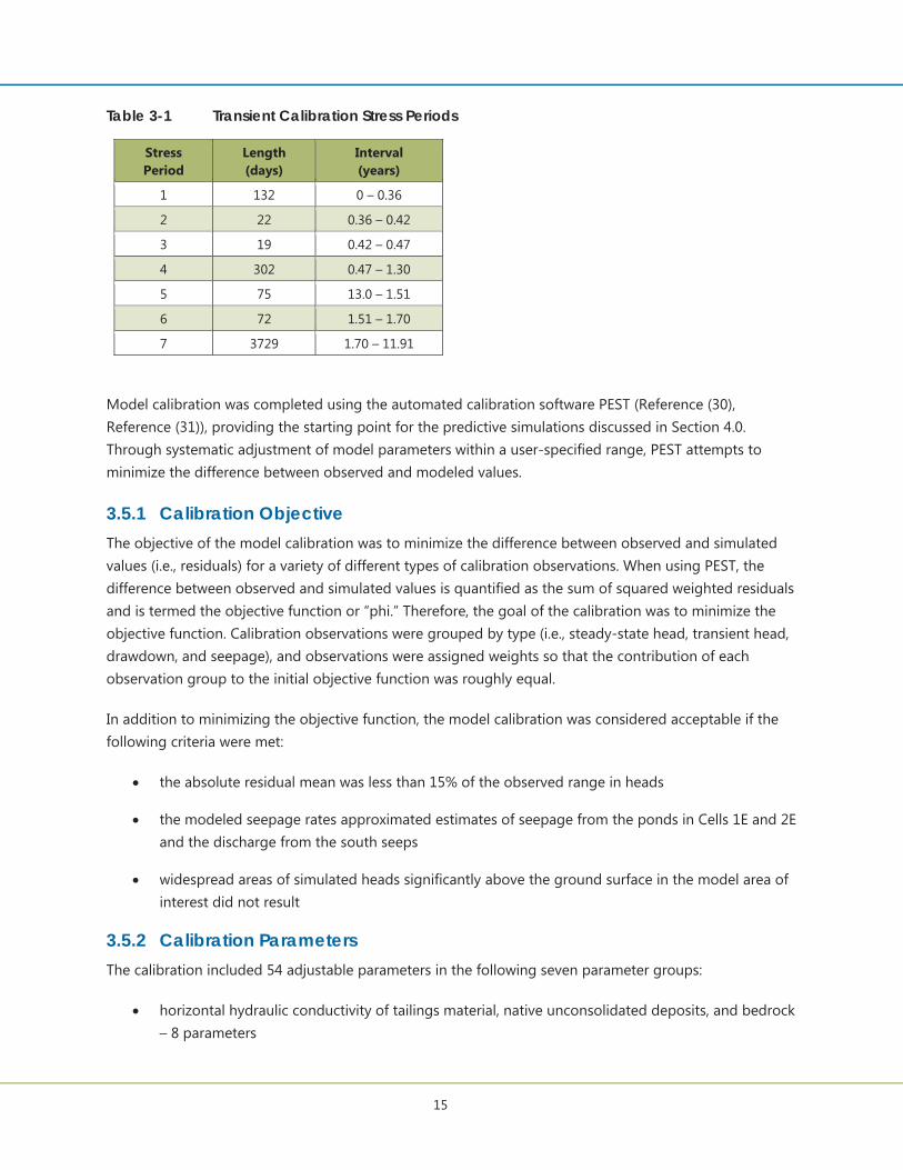
The heads from the steady-state portion of the current conditions simulation were then used as the initial heads for the transient portion of the simulation. The transient portion of the simulation spans 3,729 days (11.9 years) between February 1, 2002 and December 31, 2013 and is subdivided into seven stress periods (Table 3-1). The stress periods were defined based on measured pond elevations from the East Range Hydrology Study (Reference (26)), which includes data through 2003, and were chosen to coincide with periods of time with minimal pond level fluctuation. The period from 2003 to the end of 2013 was simulated using a single stress period.

15

Table 3-1 Transient Calibration Stress Periods

Stress Period

Length (days)

Interval (years)

1 132 0 – 0.36

2 22 0.36 – 0.42

3 19 0.42 – 0.47

4 302 0.47 – 1.30

5 75 13.0 – 1.51

6 72 1.51 – 1.70

7 3729 1.70 – 11.91

Model calibration was completed using the automated calibration software PEST (Reference (30), Reference (31)), providing the starting point for the predictive simulations discussed in Section 4.0. Through systematic adjustment of model parameters within a user-specified range, PEST attempts to minimize the difference between observed and modeled values.

3.5.1 Calibration Objective The objective of the model calibration was to minimize the difference between observed and simulated values (i.e., residuals) for a variety of different types of calibration observations. When using PEST, the difference between observed and simulated values is quantified as the sum of squared weighted residuals and is termed the objective function or “phi.” Therefore, the goal of the calibration was to minimize the objective function. Calibration observations were grouped by type (i.e., steady-state head, transient head, drawdown, and seepage), and observations were assigned weights so that the contribution of each observation group to the initial objective function was roughly equal.

In addition to minimizing the objective function, the model calibration was considered acceptable if the following criteria were met:

the absolute residual mean was less than 15% of the observed range in heads

the modeled seepage rates approximated estimates of seepage from the ponds in Cells 1E and 2E and the discharge from the south seeps

widespread areas of simulated heads significantly above the ground surface in the model area of interest did not result

3.5.2 Calibration Parameters The calibration included 54 adjustable parameters in the following seven parameter groups:

horizontal hydraulic conductivity of tailings material, native unconsolidated deposits, and bedrock – 8 parameters

16

vertical hydraulic conductivity of tailings material, native unconsolidated deposits, and bedrock – 8 parameters

vertical hydraulic conductivity of wetland sediment overlaying native unconsolidated deposits and bedrock – 2 parameters

recharge – 6 parameters (2 recharge zones were only adjusted during the first transient stress period and then applied for the remaining stress periods, 4 recharge zones were adjusted during the first transient stress period and the steady-state portion of the simulation)

storage properties of tailings material, native unconsolidated deposits, and bedrock – 14 parameters (the spatial distribution of storage zones coincided with the hydraulic conductivity zones)

heads in the specified-head cells representing the ponds for each transient stress period – 14 parameters

conductance of the drain cells representing the south seeps and drain cells representing potential seeps from bedrock outcrops (as noted above, conductance was adjusted for one cell size, and the remaining cell conductance values were scaled by cell area) – 2 parameters

Large Table 1 contains a summary of the parameters adjusted during calibration, as well as user-supplied upper and lower limits applied by PEST and the optimized value for each parameter.

3.5.3 Calibration Data Sets The calibration observation data set included a total of 1,199 observations placed in the following 5 groups:

steady-state heads

transient heads

transient drawdowns

estimated seepage from the ponds in Cell 1E and 2E in the steady-state stress period

discharge from the south seeps

ground surface elevation data to constrain heads to be below the ground surface

Monitoring wells and piezometers with head and drawdown observations used for calibration are shown on Large Figure 9. The steady-state head observations included groundwater elevation measurements collected on or around February 2002 from monitoring wells and piezometers within and outside the footprint of the Tailings Basin (Large Table 2). The transient head observation group primarily included groundwater elevations measured in monitoring wells located outside the footprint of the Tailings Basin (GW001, GW002, GW006 through GW016) after February 2002 through 2013 (Large Table 3). Systematic

17

drawdown was not observed at these wells because they are not located within the Tailings Basin, so they were not included in the drawdown group. Transient head observations were included for GW005, which is located within the footprint of the Tailings Basin, to help constrain head values in this area of the model. The transient drawdown observations group included drawdown calculated based on water levels measured since 2002 in a total of 29 monitoring wells and piezometers located within the footprint of the Tailings Basin (Large Table 4).

In addition to measured heads and drawdowns, the model calibration attempted to match estimated seepage losses from the ponds within Cell 1E and Cell 2E and measured seepage rates at the south seeps. The East Range Hydrology Project (Reference (26)) used a water-balance model, WATBUD, to simulate the hydrology of the Cell 1E and Cell 2E ponds. Net groundwater seepage losses were estimated to be 1.53 cubic feet per second (cfs) and 2.00 cfs for Cells 1E and 2E, respectively. While the East Range Hydrology Project included data through 2003, the seepage estimates were assumed to be representative of the period that coincided with the steady-state stress period of the MODFLOW model (Reference (26)). Seepage rates for the two main seeps located south of Cell 1E have been measured periodically since 2002. A flow rate of 471 gallons per minute (gpm), which represents an average seepage rate based on data collected from NPDES permit monitoring location SD026 (located downstream of the south seeps) between February 2002 and June 2011, was used for the seepage estimate in the calibration. Measured flow rates at SD026 after June 2011 are not representative of the conditions being modeled because a pump-back system was installed in July 2011, which collects water from the south seeps and returns it to the pond in Cell 1E.

Calibration observations were assigned weights so that the contribution of each observation group to the initial objective function was roughly equal. Some observations were assigned slightly higher weights in order to produce a calibrated model that better simulated those observations. Weights were varied between individual observations within some observation groups to reflect differing levels of data quality. Of the original 1,199 observations, a total of 90 were assigned zero weight, which removes them from consideration during the calibration (i.e., PEST does not attempt to match them). All of the zero-weight observations were in the transient drawdown group. The drawdown observations that were assigned zero weight are shown on transient drawdown plots (discussed below) and generally represent observations that are inconsistent with other observations at that location. In some cases, all observations at a given location were assigned a zero weight because observations were inconsistent with nearby locations or the observations were otherwise anomalous and could not be matched by the model. For example, water levels observed at piezometer DH96-30 were consistent with other piezometers within the footprint of the Tailings Basin from 2002 until mid-2004, but starting in mid-2004, an abrupt increase in water levels was observed, which is inconsistent with other nearby piezometers. Therefore, these observations were assigned zero weight. Water levels at P3H1-99 did not decrease over time, unlike nearby piezometers, so all observations from this location were assigned zero weight.

Information was also added to the calibration to minimize areas with simulated heads significantly above the ground surface. Head observations (i.e., control points) were added at seventeen locations across the model domain (Large Figure 9) with the target head set equal to the estimated ground surface (top

18

elevation of Layer 2). One steady-state and one transient head observation (at the end of the transient simulation) were assigned at each location.

3.5.4 Regularization and Prior Information In addition to observations and estimates based on field data, automated calibration using PEST may be guided by additional user-supplied information related to the calibration parameters, known as “regularization information” and “prior information.” Regularization and prior information do not impose a hard constraint on the parameter values; rather, PEST will attempt to honor the information to the extent possible and a “penalty” will be added to the objective function if the values deviate from the preferred values. Regularization information is not based directly on site-specific measurements, but reflects constraints that the calibration should honor, if possible. Prior information consists of independent estimates of parameter values based on measurements made within the model domain. The following additional information was incorporated into the calibration:

Regularization information specifying that the ratio of vertical hydraulic conductivity to horizontal hydraulic conductivity in each hydraulic conductivity zone should be less than or equal to one. Initial attempts at calibration without this constraint resulted in optimized vertical hydraulic conductivity values for some materials that far exceeded the horizontal hydraulic conductivity, which is not realistic in settings where deposits are horizontally stratified.

Prior information specifying that the horizontal hydraulic conductivity of the native unconsolidated deposits should be equal to 13.1 feet/day, the average hydraulic conductivity value estimated from in-situ pumping tests conducted in onsite wells in 2009 (Section 2.1.1).

Prior information specifying that the horizontal hydraulic conductivity of the fine and coarse LTVSMC tailings material should be equal to 0.056 feet/day and 6.9 feet/day, respectively. These hydraulic conductivity estimates are based on values used in geotechnical modeling of the Tailings Basin as described in Section 2.1.2 and Reference (12).

An “observation” of mass balance error during the calibration process. Following each model run, the maximum absolute value of the mass balance error for each time step and stress period reported in the model output files was provided to PEST as an observation with a specified value of zero. Therefore, if non-zero mass balance error was observed during the calibration process, it contributed to the objective function, which PEST attempted to minimize.

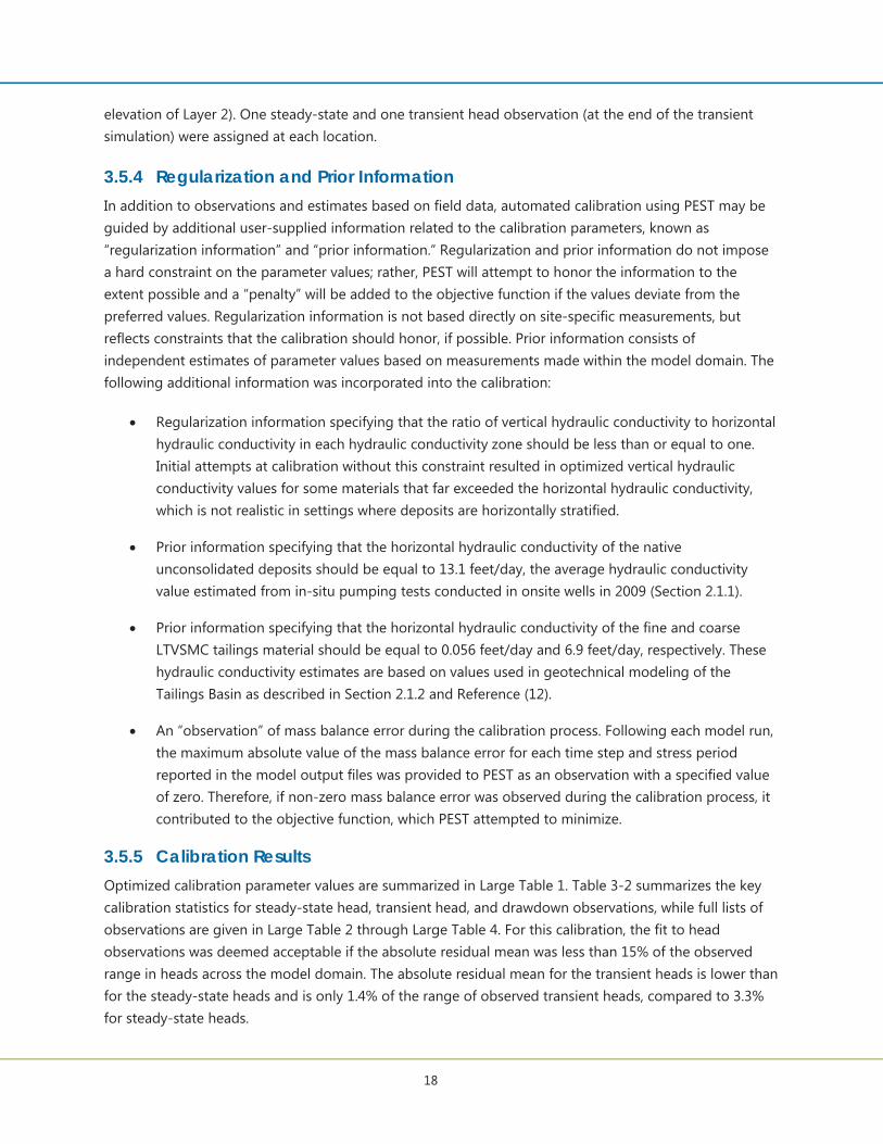
3.5.5 Calibration Results Optimized calibration parameter values are summarized in Large Table 1. Table 3-2 summarizes the key calibration statistics for steady-state head, transient head, and drawdown observations, while full lists of observations are given in Large Table 2 through Large Table 4. For this calibration, the fit to head observations was deemed acceptable if the absolute residual mean was less than 15% of the observed range in heads across the model domain. The absolute residual mean for the transient heads is lower than for the steady-state heads and is only 1.4% of the range of observed transient heads, compared to 3.3% for steady-state heads.

19

Table 3-2 Calibration Statistics for Observations

Statistics Steady-state Head Transient Head Drawdown

Range in Observed Data (feet) 298.9 380.0 27.3

Residual Mean (feet) 0.9 1.0 1.1

Abs Residual Mean (feet) 9.7 5.3 2.1

Max Abs Residual (feet) 25.1 26.3 12.9

Abs Residual Mean / Range (%) 3.3 1.4 7.7

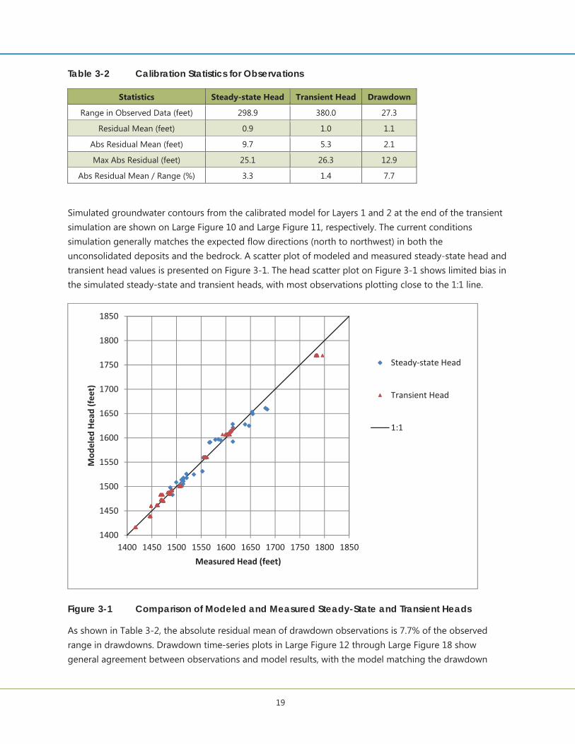
Simulated groundwater contours from the calibrated model for Layers 1 and 2 at the end of the transient simulation are shown on Large Figure 10 and Large Figure 11, respectively. The current conditions simulation generally matches the expected flow directions (north to northwest) in both the unconsolidated deposits and the bedrock. A scatter plot of modeled and measured steady-state head and transient head values is presented on Figure 3-1. The head scatter plot on Figure 3-1 shows limited bias in the simulated steady-state and transient heads, with most observations plotting close to the 1:1 line.

Figure 3-1 Comparison of Modeled and Measured Steady-State and Transient Heads

As shown in Table 3-2, the absolute residual mean of drawdown observations is 7.7% of the observed range in drawdowns. Drawdown time-series plots in Large Figure 12 through Large Figure 18 show general agreement between observations and model results, with the model matching the drawdown

1400

1450

1500

1550

1600

1650

1700

1750

1800

1850

1400 1450 1500 1550 1600 1650 1700 1750 1800 1850

Mod

eled

Head

(feet)

Measured Head (feet)

Steady state Head

Transient Head

1:1

20

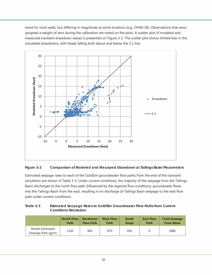
trend for most wells, but differing in magnitude at some locations (e.g., DH96-28). Observations that were assigned a weight of zero during the calibration are noted on the plots. A scatter plot of modeled and measured transient drawdown values is presented on Figure 3-2. The scatter plot shows limited bias in the simulated drawdowns, with heads falling both above and below the 1:1 line.

Figure 3-2 Comparison of Modeled and Measured Drawdown at Tailings Basin Piezometers

Estimated seepage rates to each of the GoldSim groundwater flow paths from the end of the transient simulation are shown in Table 3-3. Under current conditions, the majority of the seepage from the Tailings Basin discharges to the north flow path. Influenced by the regional flow conditions, groundwater flows into the Tailings Basin from the east, resulting in no discharge of Tailings Basin seepage to the east flow path under current conditions.

Table 3-3 Estimated Seepage Rates to GoldSim Groundwater Flow Paths from Current Conditions Simulation

North Flow

Path Northwest Flow Path

West Flow Path

South Seeps

East Flow Path

Total Seepage From Basin

Model-Estimated Seepage Rate (gpm)

1100 460 870 450 0 2880

10

5

0

5

10

15

20

25

30

10 5 0 5 10 15 20 25 30

Mod

eled

Draw

down(fe

et)

Measured Drawdown (feet)

Drawdown

1:1

21

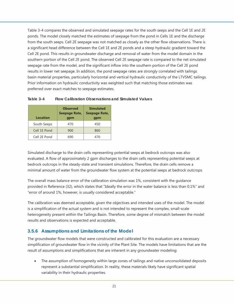
Table 3-4 compares the observed and simulated seepage rates for the south seeps and the Cell 1E and 2E ponds. The model closely matched the estimates of seepage from the pond in Cells 1E and the discharge from the south seeps. Cell 2E seepage was not matched as closely as the other flow observations. There is a significant head difference between the Cell 1E and 2E ponds and a steep hydraulic gradient toward the Cell 2E pond. This results in groundwater discharge and removal of water from the model domain in the southern portion of the Cell 2E pond. The observed Cell 2E seepage rate is compared to the net simulated seepage rate from the model, and the significant inflow into the southern portion of the Cell 2E pond results in lower net seepage. In addition, the pond seepage rates are strongly correlated with tailings basin material properties, particularly horizontal and vertical hydraulic conductivity of the LTVSMC tailings. Prior information on hydraulic conductivity was weighted such that matching those estimates was preferred over exact matches to seepage estimates.

Table 3-4 Flow Calibration Observations and Simulated Values

Location

Observed Seepage Rate,

gpm

Simulated Seepage Rate,

gpm

South Seeps 470 450

Cell 1E Pond 900 860

Cell 2E Pond 690 470

Simulated discharge to the drain cells representing potential seeps at bedrock outcrops was also evaluated. A flow of approximately 2 gpm discharges to the drain cells representing potential seeps at bedrock outcrops in the steady-state and transient simulations. Therefore, the drain cells remove a minimal amount of water from the groundwater flow system at the potential seeps at bedrock outcrops.

The overall mass balance error of the calibration simulation was 1%, consistent with the guidance provided in Reference (32), which states that “Ideally the error in the water balance is less than 0.1%” and “error of around 1%, however, is usually considered acceptable.”

The calibration was deemed acceptable, given the objectives and intended uses of the model. The model is a simplification of the actual system and is not intended to represent the complex, small-scale heterogeneity present within the Tailings Basin. Therefore, some degree of mismatch between the model results and observations is expected and acceptable.

3.5.6 Assumptions and Limitations of the Model The groundwater flow models that were constructed and calibrated for this evaluation are a necessary simplification of groundwater flow in the vicinity of the Plant Site. The models have limitations that are the result of assumptions and simplifications that are inherent in any groundwater modeling:

The assumption of homogeneity within large zones of tailings and native unconsolidated deposits represent a substantial simplification. In reality, these materials likely have significant spatial variability in their hydraulic properties.

22

The use of a conventional porous media modeling code can accurately simulate flow within the bedrock outcrops near the Tailings Basin, which is assumed to be primarily through interconnected fractures, at the scale of this study. It is assumed that the fractures are sufficiently interconnected such that the fractured rock medium behaves similar to a porous medium.

The validity of the modeling results is based on the assumption that the conceptual model is a reasonable representation of the groundwater flow system. The conceptual model, in turn, is based on the data that were collected at the Plant Site and the interpretation of those data. Errors in the data or data interpretation that affect the groundwater flow model’s conceptualization may result in errors in the flow simulation.

The artificially high recharge rates applied to Cell 2W tailings for the steady-state portion of the simulation were necessary to reproduce observed conditions prior to the transient portion of the simulation but do not reflect actual recharge rates anticipated during that time period. Using a steady-state simulation to set the initial conditions for a transient simulation is standard practice (Reference (32)).

The groundwater flow model was designed with the specific goals summarized in Section 1.1. If the model is to be used for other purposes, the validity of the model for that purpose must be carefully evaluated.

23

4.0 Predictive Simulations The calibrated current conditions models were used to develop Tailings Basin simulations representing operations conditions (Mine Year 1 through Mine Year 20) and long-term closure conditions (after Mine Year 55, when reclamation activities are complete). The primary objectives of the predictive simulations were to estimate the quantity of seepage from the Tailings Basin and Tailings Basin ponds, estimate the contribution of infiltration from each the various areas of the Tailings Basin to each of the groundwater flow paths simulated in the GoldSim model, and estimate the unsaturated zone thickness at the Tailings Basin to support calculations of oxygen penetration depth in the GoldSim model (Reference (1)).

A series of steady-state simulations were set up to represent conditions within the Tailings Basin at key times during operations:

Mine Year 1 (Large Figure 19). Tailings deposition will begin in Cell 2E in the first year of operations. Tailings will be deposited both on the exposed beaches and within the pond.

Mine Year 7 (Large Figure 20). Mine Year 7 represents the last year in which tailings will be deposited only in Cell 2E.

Mine Year 8 (Large Figure 21). After approximately seven years of depositing tailings in Cell 2E, the elevation of the cell will reach the elevation of Cell 1E, and the two will merge. From approximately Mine Year 8 through Mine Year 20, tailings will be deposited in the merged cells (FTB Pond).

Mine Year 18 (Large Figure 22). The dams are expanded in Mine Year 18, and the beach fully encompasses the FTB Pond.

Mine Year 20 (Large Figure 22). The Tailings Basin reaches its final height in Mine Year 20.

The model results at the end of the Mine Year 20 simulation were used as the starting point for simulations to evaluate long-term closure conditions. Achieving water quality objectives at the Tailings Basin during long-term closure will depend in part on maintaining proper moisture conditions and oxygen exclusion in the Flotation Tailings. This will be accomplished by maintenance of a pond above much of the Flotation Tailings following closure (Section 5.0 of Reference (33)). The pond will simultaneously prevent oxygen intrusion from the tailings surface, while also providing water to maintain elevated saturation conditions in tailings below the pond. Because the seepage through the Flotation Tailings in combination with the small area providing surface water runoff to the basin may make it difficult to maintain a pond during some portions of the year, the permeability of the tailings at the surface will be modified by bentonite addition as needed to reduce the hydraulic conductivity of the tailings. The reduced hydraulic conductivity will limit seepage through the tailings and will result in maintenance of a pond above the tailings after basin closure.

Predictive simulations of operation conditions were steady-state. Linear interpolation was used between the simulated years to provide estimates on an annual basis for inputs to the GoldSim model. Two

24

simulations of long-term closure conditions were completed: a steady-state simulation to provide input for the GoldSim model and a transient simulation to estimate the time required for the system to reach a steady state following closure. The following sections describe the aspects of the current conditions model that were modified to set up the predictive simulations.

4.1 Modifications to the Current Conditions Model 4.1.1 Model Layers Model layers were added to the current conditions model to represent the increasing thickness of Flotation Tailings as they will be deposited during operations. In general, Flotation Tailings thickness will increase more rapidly in earlier years compared to later years, in part because the area of Flotation tailings deposition is smaller prior to Mine Year 8 when the tailings are deposited exclusively in Cell 2E. For the Mine Year 1 simulation, two additional layers were added, resulting in a total of four model layers. For the Mine Year 7 simulation, an additional three model layers were added to the Mine Year 1 simulation (for a total of seven model layers). No additional model layers were added for the Mine Year 8 simulation. One additional layer was added for the Mine Year 18, Mine Year 20, and long-term closure conditions simulations, resulting in a total of eight layers. As with the current conditions models, the bottom model layer for the predictive simulations represents the native unconsolidated deposits and bedrock hills.

For each new model layer added in all simulations, the extent of active cells was defined based on the Tailings Basin design as shown on Large Figure 19 through Large Figure 22.

4.1.2 Boundary Conditions During operations, the ponds in Cell 1E and 2E (and the combined FTB Pond starting in Mine Year 8) were represented using specified-head boundaries. For the closure simulation, the pond was represented using river cells. The use of river cell boundaries to simulate the pond following closure was based on the assumption that the pond will be lined with an 18-inch-thick layer of bentonite that has distinct properties from the underlying tailings (Section 5.0 of Reference (33)). River cells were used instead of specified-head cells in closure because river cells can simulate the flux through a low hydraulic conductivity pond bottom without requiring the addition of a new layer to explicitly represent it. The bottom elevation of the river cells was defined so that the pond depth in closure would be 8 feet. The vertical hydraulic conductivity of the river cells was assigned as 2.8 x 10-4 feet/day to simulate the anticipated hydraulic conductivity of the bentonite layer (Reference (33)).

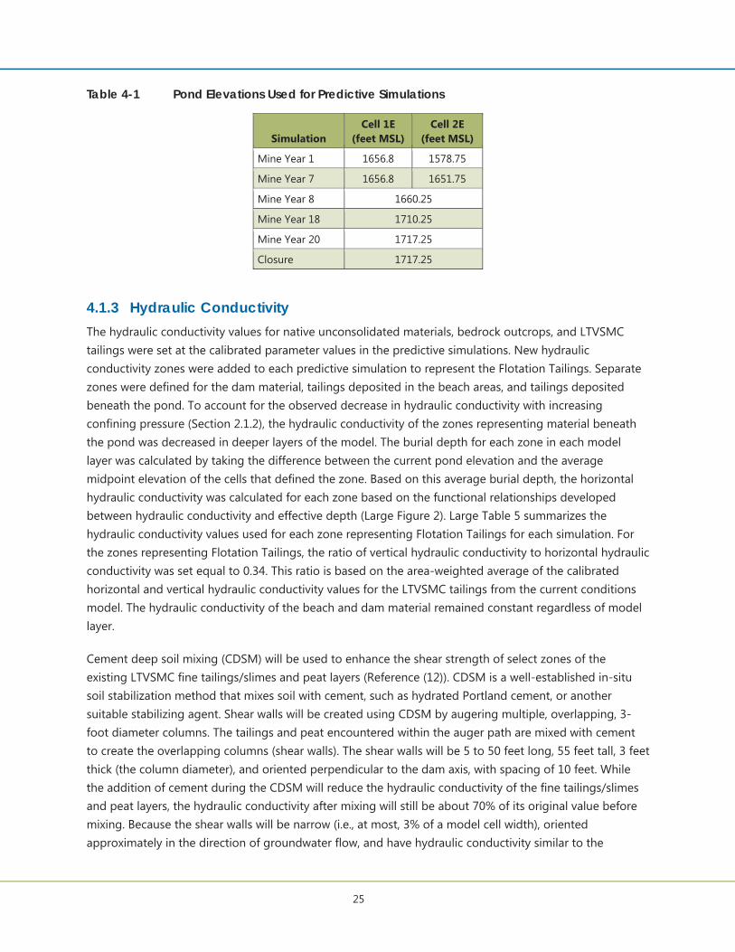
For each predictive simulation, the spatial extent of the specified-head cells or river cells and the head assigned to each pond were based on the current version of the FTB design (Reference (5))). The specified-head cells representing the FTB design for each year simulated is shown on Large Figure 23 through Large Figure 26. The pond elevation was assumed to be 9.25 feet below the top of dam elevation for each of the years simulated. Table 4-1 summarizes the elevations applied to the specified-head cells or river cells representing the ponds for each simulation. Large Figure 27 shows the boundary conditions in the bottom model layer for each predictive simulation.

25

Table 4-1 Pond Elevations Used for Predictive Simulations

Simulation Cell 1E

(feet MSL) Cell 2E

(feet MSL)

Mine Year 1 1656.8 1578.75

Mine Year 7 1656.8 1651.75

Mine Year 8 1660.25

Mine Year 18 1710.25

Mine Year 20 1717.25

Closure 1717.25

4.1.3 Hydraulic Conductivity The hydraulic conductivity values for native unconsolidated materials, bedrock outcrops, and LTVSMC tailings were set at the calibrated parameter values in the predictive simulations. New hydraulic conductivity zones were added to each predictive simulation to represent the Flotation Tailings. Separate zones were defined for the dam material, tailings deposited in the beach areas, and tailings deposited beneath the pond. To account for the observed decrease in hydraulic conductivity with increasing confining pressure (Section 2.1.2), the hydraulic conductivity of the zones representing material beneath the pond was decreased in deeper layers of the model. The burial depth for each zone in each model layer was calculated by taking the difference between the current pond elevation and the average midpoint elevation of the cells that defined the zone. Based on this average burial depth, the horizontal hydraulic conductivity was calculated for each zone based on the functional relationships developed between hydraulic conductivity and effective depth (Large Figure 2). Large Table 5 summarizes the hydraulic conductivity values used for each zone representing Flotation Tailings for each simulation. For the zones representing Flotation Tailings, the ratio of vertical hydraulic conductivity to horizontal hydraulic conductivity was set equal to 0.34. This ratio is based on the area-weighted average of the calibrated horizontal and vertical hydraulic conductivity values for the LTVSMC tailings from the current conditions model. The hydraulic conductivity of the beach and dam material remained constant regardless of model layer.

Cement deep soil mixing (CDSM) will be used to enhance the shear strength of select zones of the existing LTVSMC fine tailings/slimes and peat layers (Reference (12)). CDSM is a well-established in-situ soil stabilization method that mixes soil with cement, such as hydrated Portland cement, or another suitable stabilizing agent. Shear walls will be created using CDSM by augering multiple, overlapping, 3-foot diameter columns. The tailings and peat encountered within the auger path are mixed with cement to create the overlapping columns (shear walls). The shear walls will be 5 to 50 feet long, 55 feet tall, 3 feet thick (the column diameter), and oriented perpendicular to the dam axis, with spacing of 10 feet. While the addition of cement during the CDSM will reduce the hydraulic conductivity of the fine tailings/slimes and peat layers, the hydraulic conductivity after mixing will still be about 70% of its original value before mixing. Because the shear walls will be narrow (i.e., at most, 3% of a model cell width), oriented approximately in the direction of groundwater flow, and have hydraulic conductivity similar to the

26

materials prior to mixing, the shear walls were not simulated in the groundwater model as they are not expected to have a significant impact on the key model predictions.

4.1.4 RechargeFor the predictive simulations, the following recharge zones were added to the model:

a zone representing infiltration through the exterior FTB dams, which will be covered with bentonite starting in Mine Year 1

a zone representing infiltration through the beach areas during operations

a zone representing infiltration through the beach areas during long-term closure, after they have been amended with bentonite

The spatial extent of each zone in each simulation was determined using the FTB design. Recharge rates for the zone representing infiltration through the beach areas for each simulation were calculated as an area- and time-weighted average that accounts for the infiltration from the tailings slurry and natural infiltration rates from precipitation estimated using the Meyer Model (Reference (20)). A more detailed description of the procedure follows.

The procedure for calculating infiltration rates to inactive beach areas and the covered dams are described in Section 5.2.2.2.2 of Reference (1)). In those areas, infiltration is equal to precipitation less runoff and evapotranspiration. For the inactive beaches during operations, the infiltration rate averages approximately 7.7 in/yr. For the beaches in closure and the dams at all times, the infiltration rate averages about 5.85 in/yr. At any time, the Beneficiation Plant (Plant) will discharge along the dams to form tailings beaches. As the Plant discharges to a beach, the slurry spreads over a portion of a delta that is assumed to cover 2.06 acres (Section 5.2.2.2.2 of Reference (1)). The slurry discharge rate to the beach is high enough that the infiltration rate over the 2.06 acres is assumed to be equal to the saturated hydraulic conductivity of the beach tailings, which is about 2.8 feet/day (see Section 10.3.2 of Reference (34)). Equation 3 represents the spatial average infiltration rate of a beach that is receiving Plant slurry discharge.

Equation 3

Where:

IA is the spatially averaged infiltration rate [L/T] Ksat is the saturated hydraulic conductivity [L/T] IC is the average infiltration rate due to natural climate [L/T] Ai is the entire area of a single beach [L2], and AD is the area of the delta with flowing slurry [L2].

Equation 3 will approach IC as Ai gets very large.

Because the Plant will discharge to one beach at a time, there are times during the year when IA will be very high and other times when it will be equal to IC (because AD = 0 acres). Equation 4 is used to

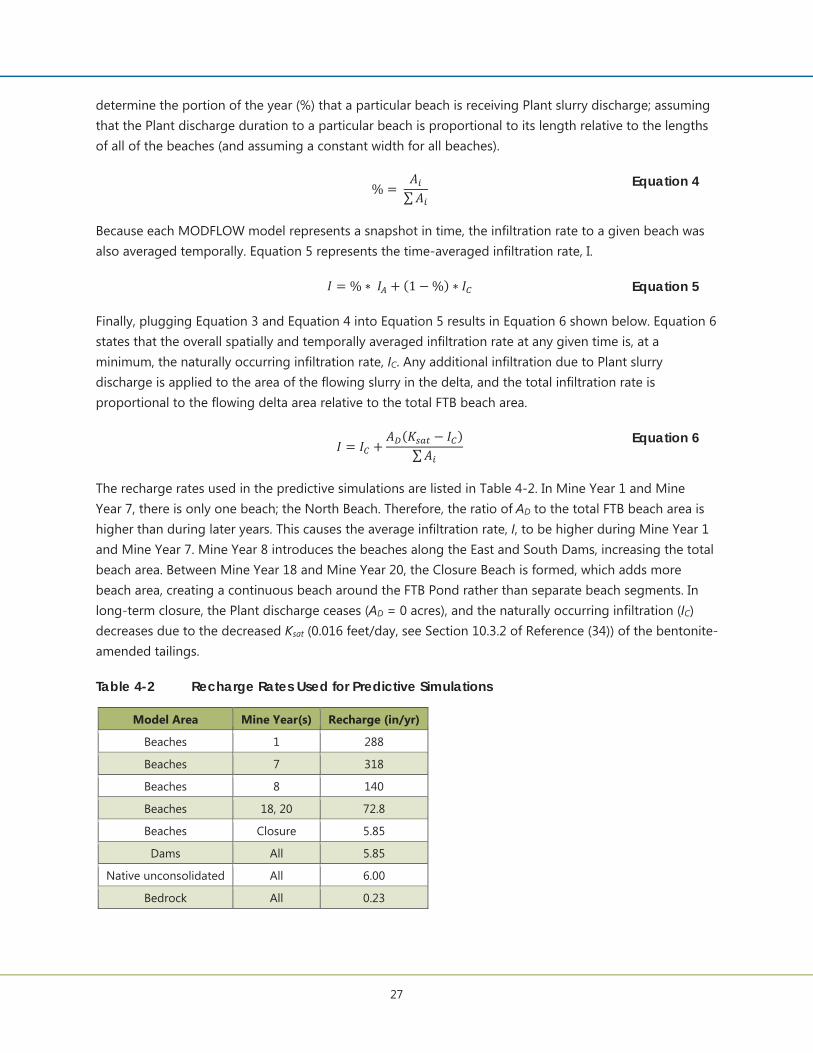
27

determine the portion of the year (%) that a particular beach is receiving Plant slurry discharge; assuming that the Plant discharge duration to a particular beach is proportional to its length relative to the lengths of all of the beaches (and assuming a constant width for all beaches).

Equation 4

Because each MODFLOW model represents a snapshot in time, the infiltration rate to a given beach was also averaged temporally. Equation 5 represents the time-averaged infiltration rate, I.

Equation 5

Finally, plugging Equation 3 and Equation 4 into Equation 5 results in Equation 6 shown below. Equation 6 states that the overall spatially and temporally averaged infiltration rate at any given time is, at a minimum, the naturally occurring infiltration rate, IC. Any additional infiltration due to Plant slurry discharge is applied to the area of the flowing slurry in the delta, and the total infiltration rate is proportional to the flowing delta area relative to the total FTB beach area.

Equation 6

The recharge rates used in the predictive simulations are listed in Table 4-2. In Mine Year 1 and Mine Year 7, there is only one beach; the North Beach. Therefore, the ratio of AD to the total FTB beach area is higher than during later years. This causes the average infiltration rate, I, to be higher during Mine Year 1 and Mine Year 7. Mine Year 8 introduces the beaches along the East and South Dams, increasing the total beach area. Between Mine Year 18 and Mine Year 20, the Closure Beach is formed, which adds more beach area, creating a continuous beach around the FTB Pond rather than separate beach segments. In long-term closure, the Plant discharge ceases (AD = 0 acres), and the naturally occurring infiltration (IC) decreases due to the decreased Ksat (0.016 feet/day, see Section 10.3.2 of Reference (34)) of the bentonite-amended tailings.

Table 4-2 Recharge Rates Used for Predictive Simulations

Model Area Mine Year(s) Recharge (in/yr)

Beaches 1 288

Beaches 7 318

Beaches 8 140

Beaches 18, 20 72.8

Beaches Closure 5.85

Dams All 5.85

Native unconsolidated All 6.00

Bedrock All 0.23

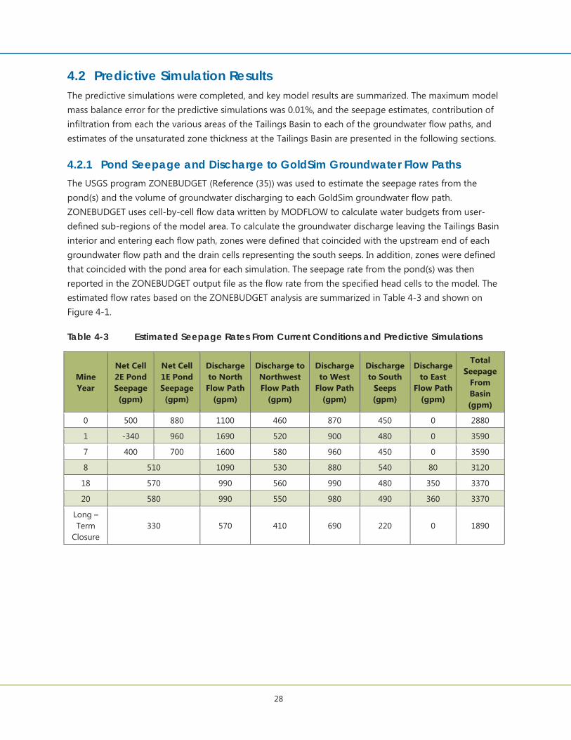
28

4.2 Predictive Simulation Results The predictive simulations were completed, and key model results are summarized. The maximum model mass balance error for the predictive simulations was 0.01%, and the seepage estimates, contribution of infiltration from each the various areas of the Tailings Basin to each of the groundwater flow paths, and estimates of the unsaturated zone thickness at the Tailings Basin are presented in the following sections.

4.2.1 Pond Seepage and Discharge to GoldSim Groundwater Flow Paths The USGS program ZONEBUDGET (Reference (35)) was used to estimate the seepage rates from the pond(s) and the volume of groundwater discharging to each GoldSim groundwater flow path. ZONEBUDGET uses cell-by-cell flow data written by MODFLOW to calculate water budgets from user-defined sub-regions of the model area. To calculate the groundwater discharge leaving the Tailings Basin interior and entering each flow path, zones were defined that coincided with the upstream end of each groundwater flow path and the drain cells representing the south seeps. In addition, zones were defined that coincided with the pond area for each simulation. The seepage rate from the pond(s) was then reported in the ZONEBUDGET output file as the flow rate from the specified head cells to the model. The estimated flow rates based on the ZONEBUDGET analysis are summarized in Table 4-3 and shown on Figure 4-1.

Table 4-3 Estimated Seepage Rates From Current Conditions and Predictive Simulations

Mine Year

Net Cell 2E Pond Seepage (gpm)

Net Cell 1E Pond Seepage (gpm)

Discharge to North

Flow Path (gpm)

Discharge to Northwest Flow Path

(gpm)

Discharge to West

Flow Path (gpm)

Discharge to South

Seeps (gpm)

Discharge to East

Flow Path (gpm)

Total Seepage

From Basin (gpm)

0 500 880 1100 460 870 450 0 2880

1 -340 960 1690 520 900 480 0 3590

7 400 700 1600 580 960 450 0 3590

8 510 1090 530 880 540 80 3120

18 570 990 560 990 480 350 3370

20 580 990 550 980 490 360 3370

Long –Term

Closure 330 570 410 690 220 0 1890

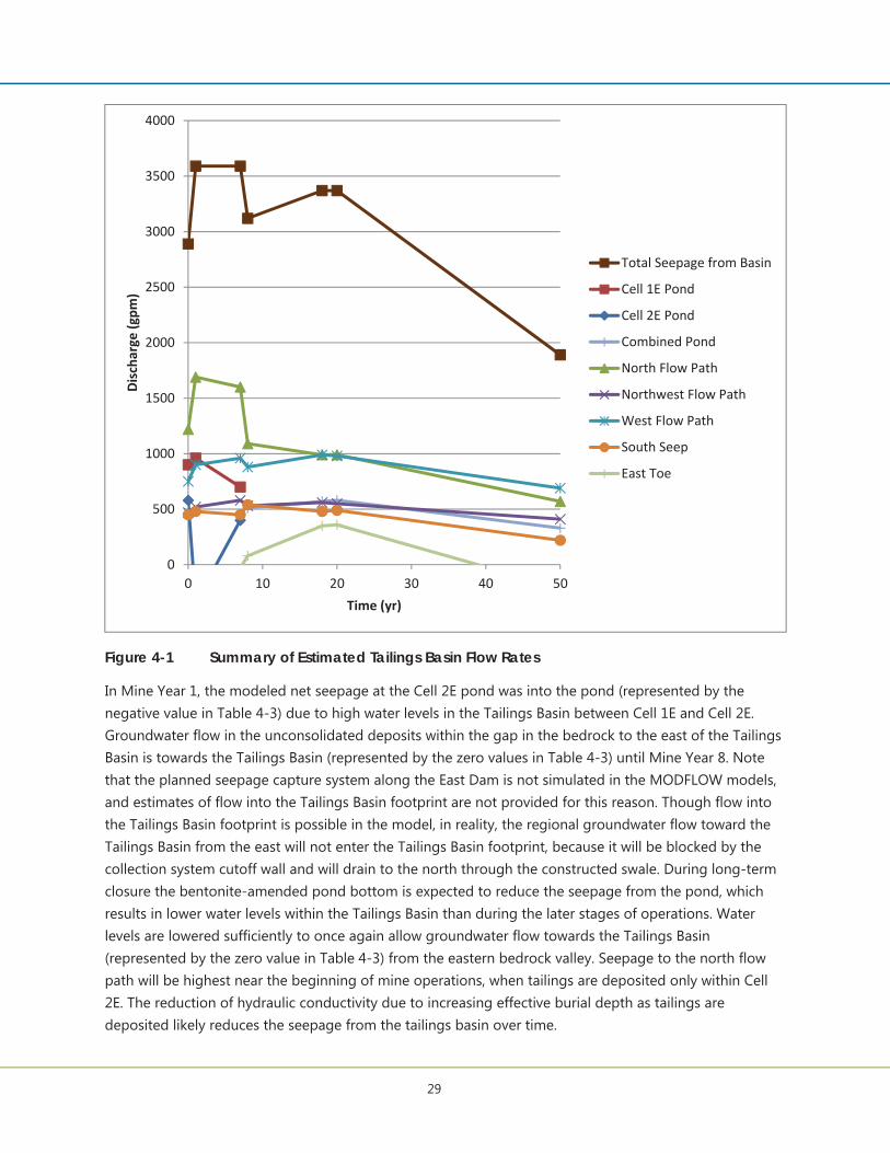
29

Figure 4-1 Summary of Estimated Tailings Basin Flow Rates

In Mine Year 1, the modeled net seepage at the Cell 2E pond was into the pond (represented by the negative value in Table 4-3) due to high water levels in the Tailings Basin between Cell 1E and Cell 2E. Groundwater flow in the unconsolidated deposits within the gap in the bedrock to the east of the Tailings Basin is towards the Tailings Basin (represented by the zero values in Table 4-3) until Mine Year 8. Note that the planned seepage capture system along the East Dam is not simulated in the MODFLOW models, and estimates of flow into the Tailings Basin footprint are not provided for this reason. Though flow into the Tailings Basin footprint is possible in the model, in reality, the regional groundwater flow toward the Tailings Basin from the east will not enter the Tailings Basin footprint, because it will be blocked by the collection system cutoff wall and will drain to the north through the constructed swale. During long-term closure the bentonite-amended pond bottom is expected to reduce the seepage from the pond, which results in lower water levels within the Tailings Basin than during the later stages of operations. Water levels are lowered sufficiently to once again allow groundwater flow towards the Tailings Basin (represented by the zero value in Table 4-3) from the eastern bedrock valley. Seepage to the north flow path will be highest near the beginning of mine operations, when tailings are deposited only within Cell 2E. The reduction of hydraulic conductivity due to increasing effective burial depth as tailings are deposited likely reduces the seepage from the tailings basin over time.

0

500

1000

1500

2000

2500

3000

3500

4000

0 10 20 30 40 50

Discha

rge(gpm

)

Time (yr)

Total Seepage from Basin

Cell 1E Pond

Cell 2E Pond

Combined Pond

North Flow Path

Northwest Flow Path

West Flow Path

South Seep

East Toe

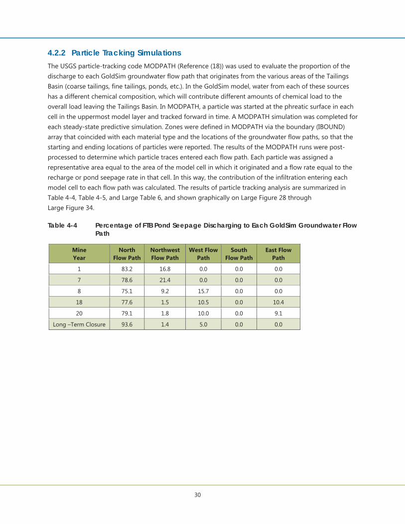
30

4.2.2 Particle Tracking Simulations The USGS particle-tracking code MODPATH (Reference (18)) was used to evaluate the proportion of the discharge to each GoldSim groundwater flow path that originates from the various areas of the Tailings Basin (coarse tailings, fine tailings, ponds, etc.). In the GoldSim model, water from each of these sources has a different chemical composition, which will contribute different amounts of chemical load to the overall load leaving the Tailings Basin. In MODPATH, a particle was started at the phreatic surface in each cell in the uppermost model layer and tracked forward in time. A MODPATH simulation was completed for each steady-state predictive simulation. Zones were defined in MODPATH via the boundary (IBOUND) array that coincided with each material type and the locations of the groundwater flow paths, so that the starting and ending locations of particles were reported. The results of the MODPATH runs were post-processed to determine which particle traces entered each flow path. Each particle was assigned a representative area equal to the area of the model cell in which it originated and a flow rate equal to the recharge or pond seepage rate in that cell. In this way, the contribution of the infiltration entering each model cell to each flow path was calculated. The results of particle tracking analysis are summarized in Table 4-4, Table 4-5, and Large Table 6, and shown graphically on Large Figure 28 through Large Figure 34.

Table 4-4 Percentage of FTB Pond Seepage Discharging to Each GoldSim Groundwater Flow Path

Mine Year

North Flow Path

Northwest Flow Path

West Flow Path

South Flow Path

East Flow Path

1 83.2 16.8 0.0 0.0 0.0

7 78.6 21.4 0.0 0.0 0.0

8 75.1 9.2 15.7 0.0 0.0

18 77.6 1.5 10.5 0.0 10.4

20 79.1 1.8 10.0 0.0 9.1

Long –Term Closure 93.6 1.4 5.0 0.0 0.0

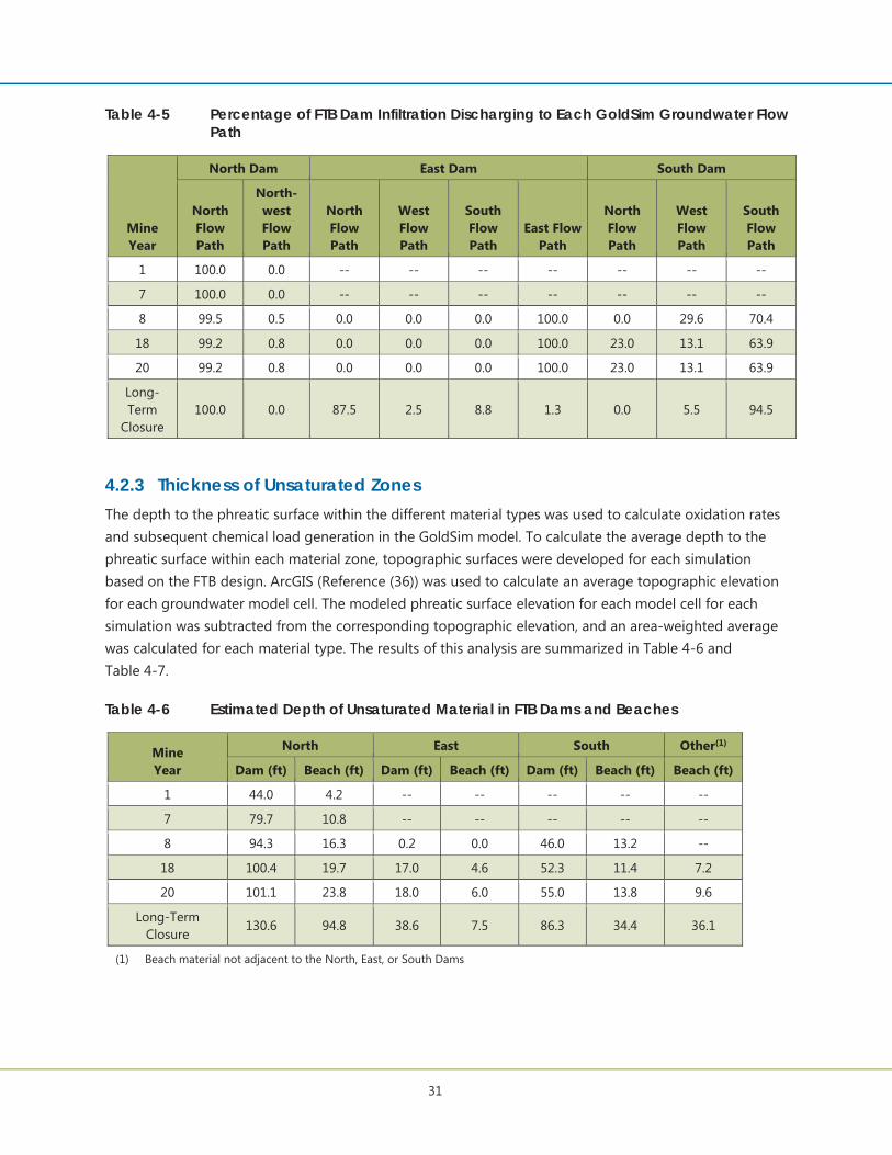
31

Table 4-5 Percentage of FTB Dam Infiltration Discharging to Each GoldSim Groundwater Flow Path

Mine Year

North Dam East Dam South Dam

North Flow Path

North-west Flow Path

North Flow Path

West Flow Path

South Flow Path

East Flow Path

North Flow Path

West Flow Path

South Flow Path

1 100.0 0.0 -- -- -- -- -- -- --

7 100.0 0.0 -- -- -- -- -- -- --

8 99.5 0.5 0.0 0.0 0.0 100.0 0.0 29.6 70.4

18 99.2 0.8 0.0 0.0 0.0 100.0 23.0 13.1 63.9

20 99.2 0.8 0.0 0.0 0.0 100.0 23.0 13.1 63.9

Long-Term

Closure 100.0 0.0 87.5 2.5 8.8 1.3 0.0 5.5 94.5

4.2.3 Thickness of Unsaturated Zones The depth to the phreatic surface within the different material types was used to calculate oxidation rates and subsequent chemical load generation in the GoldSim model. To calculate the average depth to the phreatic surface within each material zone, topographic surfaces were developed for each simulation based on the FTB design. ArcGIS (Reference (36)) was used to calculate an average topographic elevation for each groundwater model cell. The modeled phreatic surface elevation for each model cell for each simulation was subtracted from the corresponding topographic elevation, and an area-weighted average was calculated for each material type. The results of this analysis are summarized in Table 4-6 and Table 4-7.

Table 4-6 Estimated Depth of Unsaturated Material in FTB Dams and Beaches

Mine Year

North East South Other(1)

Dam (ft) Beach (ft) Dam (ft) Beach (ft) Dam (ft) Beach (ft) Beach (ft)

1 44.0 4.2 -- -- -- -- --

7 79.7 10.8 -- -- -- -- --

8 94.3 16.3 0.2 0.0 46.0 13.2 --

18 100.4 19.7 17.0 4.6 52.3 11.4 7.2

20 101.1 23.8 18.0 6.0 55.0 13.8 9.6

Long-Term Closure

130.6 94.8 38.6 7.5 86.3 34.4 36.1

(1) Beach material not adjacent to the North, East, or South Dams

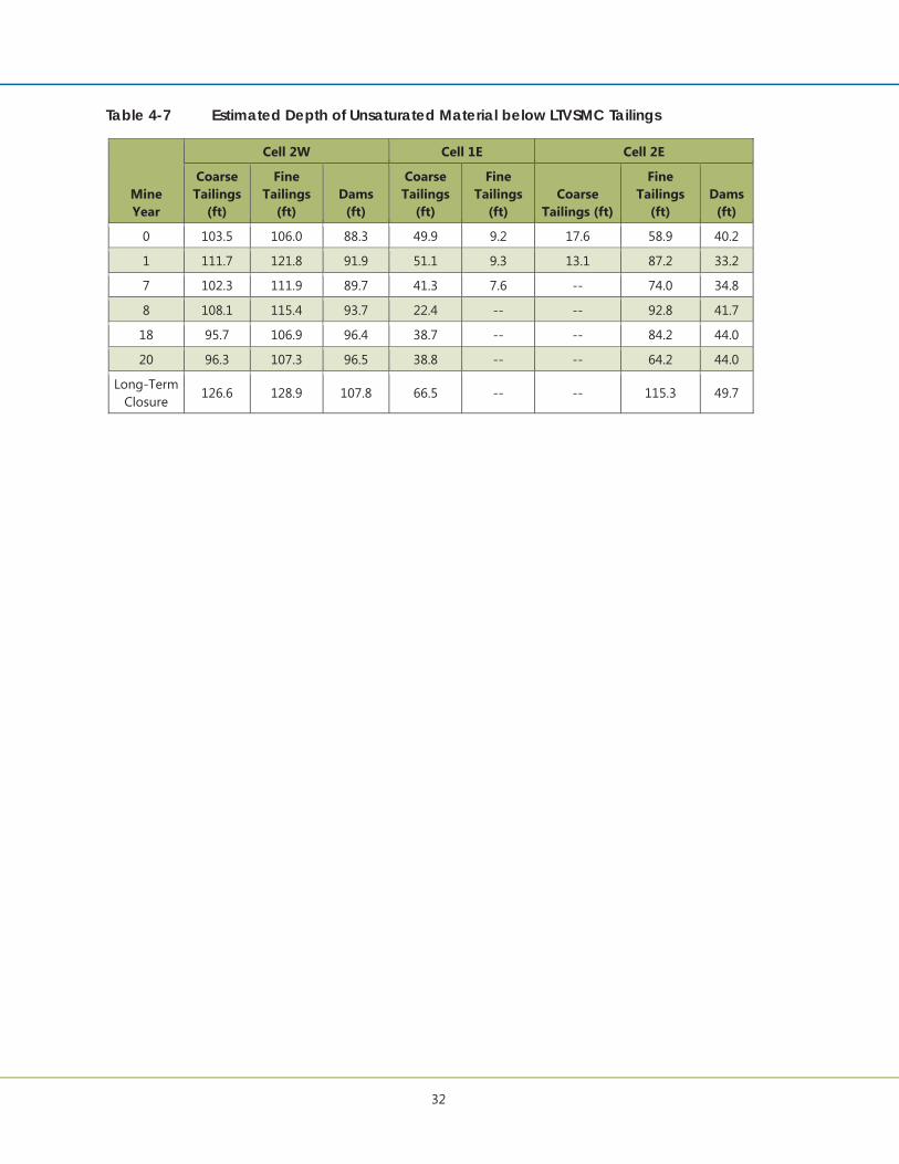
32

Table 4-7 Estimated Depth of Unsaturated Material below LTVSMC Tailings

Mine Year

Cell 2W Cell 1E Cell 2E

Coarse Tailings

(ft)

Fine Tailings

(ft) Dams

(ft)

Coarse Tailings

(ft)

Fine Tailings

(ft) Coarse

Tailings (ft)

Fine Tailings

(ft) Dams

(ft)

0 103.5 106.0 88.3 49.9 9.2 17.6 58.9 40.2

1 111.7 121.8 91.9 51.1 9.3 13.1 87.2 33.2

7 102.3 111.9 89.7 41.3 7.6 -- 74.0 34.8

8 108.1 115.4 93.7 22.4 -- -- 92.8 41.7

18 95.7 106.9 96.4 38.7 -- -- 84.2 44.0

20 96.3 107.3 96.5 38.8 -- -- 64.2 44.0

Long-Term Closure

126.6 128.9 107.8 66.5 -- -- 115.3 49.7

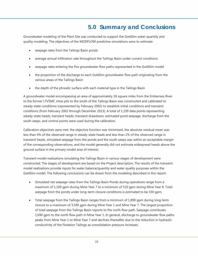
33

5.0 Summary and Conclusions Groundwater modeling of the Plant Site was conducted to support the GoldSim water quantity and quality modeling. The objectives of the MODFLOW predictive simulations were to estimate:

seepage rates from the Tailings Basin ponds

average annual infiltration rate throughout the Tailings Basin under current conditions

seepage rates entering the five groundwater flow paths represented in the GoldSim model

the proportion of the discharge to each GoldSim groundwater flow path originating from the various areas of the Tailings Basin

the depth of the phreatic surface with each material type in the Tailings Basin

A groundwater model encompassing an area of approximately 18 square miles from the Embarrass River to the former LTVSMC mine pits to the south of the Tailings Basin was constructed and calibrated to steady-state conditions (represented by February 2002) to establish initial conditions and transient conditions (from February 2002 through December 2013). A total of 1,199 data points representing steady-state heads, transient heads, transient drawdown, estimated pond seepage, discharge from the south seeps, and control points were used during the calibration.

Calibration objectives were met: the objective function was minimized, the absolute residual mean was less than 4% of the observed range in steady-state heads and less than 2% of the observed range in transient heads, simulated seepage from the ponds and the south seeps was within an acceptable margin of the corresponding observations, and the model generally did not estimate widespread heads above the ground surface in the primary model area of interest.

Transient model realizations simulating the Tailings Basin in various stages of development were constructed. The stages of development are based on the Project description. The results of the transient model realizations provide inputs for water balance/quantity and water quality purposes within the GoldSim model. The following conclusions can be drawn from the modeling described in this report:

Simulated net seepage rates from the Tailings Basin Ponds during operations range from a maximum of 1,100 gpm during Mine Year 7 to a minimum of 510 gpm during Mine Year 8. Total seepage from the ponds under long-term closure conditions is estimated to be 330 gpm.

Total seepage from the Tailings Basin ranges from a minimum of 1,890 gpm during long-term closure to a maximum of 3,590 gpm during Mine Year 1 and Mine Year 7. The largest proportion of total seepage from the Tailings Basin reports to the north flow path. Seepage contributes 1,690 gpm to the north flow path in Mine Year 1. In general, discharge to groundwater flow paths peaks from Mine Year 1 to Mine Year 7 and declines thereafter due to the reduction in hydraulic conductivity of the Flotation Tailings as consolidation pressure increases.

34

The particle tracking simulations were used to evaluate the discharge location of infiltration to the Tailings Basin and seepage from the ponds. The proportion of the discharge to each GoldSim groundwater flow path originating from the various areas of the Tailings Basin (coarse tailings, fine tailings, ponds, etc.) was tabulated for use as input to the GoldSim model.

The depth to the phreatic surface within the different material types was calculated for operations and long-term closure conditions for use in estimating oxidation rates and subsequent chemical load generation in the GoldSim model. Depths to the phreatic surface fluctuate during operations and increase following closure, due to dissipation of the groundwater mound that develops during operations.

35

6.0 References1. Poly Met Mining Inc. NorthMet Project Water Modeling Data Package Volume 2 - Plant Site (v11). January 2015.

2. —. NorthMet Project Project Description (v8). December 2014.

3. —. NorthMet Project Water Modeling Work Plan - Plant Site (v6). July 2012.

4. —. NorthMet Project Residue Management Plan (v3). November 2014.

5. —. NorthMet Project Flotation Tailings Management Plan (v4). November 2014.

6. —. NorthMet Project Water Management Plan - Plant (v3). December 2014.

7. Barr Engineering Co. Tailings Basin and Hydrometallurgical Residue Water Balance. RS13 Technical Detail Report - Draft-03. Prepared for Poly Met Mining Inc. November 16, 2007.

8. —. Hydrogeology of Fractured Bedrock in the Vicinity of the NorthMet Project (v3). December 2014.

9. Griffin, W. L. and Morey, G. B. SP-08 The Geology of the Isaac Lake Quadrangle, St. Louis County, Minnesota. s.l. : Minnesota Geological Survey, 1969.

10. Barr Engineering Co. Results of Tailings Basin Hydrogeological Investigation Technical Memorandum. Prepared for Poly Met Mining Inc. June 2, 2009.

11. Siegel, D.I. and Ericson, D.W., U.S. Geological Survey. Hydrology and Water Quality of the Copper-Nickel Study Region, Northeastern Minnesota. Water-Resources Investigations Open-File Report 80-739. 1980.

12. Poly Met Mining Inc. NorthMet Project Geotechnical Data Package Vol 1 - Flotation Tailings Basin (v5). December 2014.

13. Moench, A.F. Flow to a Well of Finite Diameter in a Homogeneous, Anisotropic Water-Table Aquifer. Water Resources Research. 1997, Vol. 33, 6, pp. 1397-1407.

14. Theis, C.V. The Relation Between Lowering of the Piezometric Surface and the Rate and Duration of Discharge of a Well Using Groundwater Storage. Transactions of the American Geophysical Union. 1935, Vol. 16, pp. 519-524.

15. Bradbury, K.B., Rothschild, E.R. A computerized technique for estimating the hydraulic conductivity of aquifer from specific capacity data. Ground Water. Vol. 23, 2, pp. 240-246.

16. Barr Engineering Co. NorthMet FTB East Dam Conceptual Model Technical Memo – Draft-02. June 20, 2014.

36

17. HydroGeoLogic, Inc. MODFLOW-SURFACT software (Version 3.0) overview: Installation, registration, and running procedures. Herndon, VA : s.n., 1996.

18. Pollock, D.W. User's Guide for MODPATH/MODPATH-PLOT, Version 3: A particle tracking post-processing package for MODFLOW, the U.S. Geological Survey finite-difference ground-water flow model, U.S. Geological Survey Open-File Report 94-464. Reston, Virginia : s.n., 1994.

19. Environmental Simulations, Inc. (ESI). Guide to Using Groundwater Vistas, Version 6. 2011.

20. Barr Engineering Co. Tailings Basin-Mitigation Design Water Balance. RS13B - Draft-01. Prepared for Poly Met Mining Inc. September 8, 2008.

21. U.S. Geological Survey. Allen Quadrangle Minnesota - St. Louis Co. 7.5 Minute Series (Topographic) Map. s.l. : U.S. Department of the Interior Geological Survey, 1949.

22. —. Aurora Quadrangle Minnesota - St. Louis Co. - 7.5 Minute Series (Topographic) Map. s.l. : U.S. Department of the Interior Geological Survey, 1949.

23. —. Embarrass Quadrangle Minnesota - St. Louis Co. 7.5 Minute Series (Topographic) Map. s.l. : U.S. Department of the Interior Geological Survey, 1949.

24. —. Isaac Lake Quadrangle Minnesota - St. Louis Co. 7.5 Minute Series (Topographic) Map. s.l. : U.S. Department of the Interior Geological Survey, 1949.

25. Jirsa, M.A., Setterholm, D.R., Bloomgren, B.A., Bauer, E.J., and Lively, R.S., University of Minnesota, Minnesota Geological Survey. Bedrock Geology Database, Bedrock Topography, Depth to Bedrock, Maps of the Eastern Half of the Mesabi Iron Range, Northern Minnesota (M-158). 2005.

26. Adams, J.L,, Leibfried, R.T. and Herr, E.S., Minnesota Deparment of Natural Resources. East Range Hydrology Project, Final Report. March 2004.

27. Poly Met Mining Inc. NorthMet Project Wetland Data Package (v9). January 2015.

28. Minnesota Department of Natural Resources (MDNR). LiDAR Elevation, Arrowhead Region. [Online] 2011. www.mngeo.state.mn.us/committee/elevation/mn_elev_mapping.html.

29. McDonald, M. G. and Harbaugh, A. W. A Modular Three-Dimensional Finite-Difference Groundwater Flow Model. U.S. Geological Survey Techniques of Water-Resource Investigations, TWRI 6-A1. 1988.

30. Watermark Numerical Computing. PEST: Model-Independent Parameter Estimation. User Manual, 5th Edition. 2005.

31. —. Addendum to the PEST Manual. 2010.

37

32. Anderson, M. P. and Woessner, W. W. Applied Groundwater Modeling: Simulation of Flow and Advective Transport. San Diego : Academic Press, Inc., 1992.

33. Poly Met Mining Inc. NorthMet Project Adaptive Water Management Plan (v6). January 2015.

34. —. NorthMet Project Waste Characterization Data Package (v11). November 2014.

35. Harbaugh, A. W. A Computer Program for Calculating Subregional Water Budgets Using Results from the U.S. Geological Survey Modular Three-dimensional Finite-difference Ground-water Flow Model, U.S. Geological Survey Open-File Report 90-392. 1990.

36. Environmental Systems Resources Institute (ESRI). ArcGIS Desktop: Release 10. Redlands, California : s.n., 2011.

Large Tables

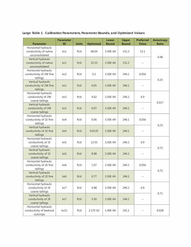
Large Table 1 Calibration Parameters, Parameter Bounds, and Optimized Values

Parameter Parameter

ID Units Optimized Lower Bound

Upper Bound

Preferred Value

Anisotropy Ratio

Horizontal hydraulic conductivity of native

unconsolidated kx1 ft/d 68.04 3.30E-04 131.2 13.1

0.48 Vertical hydraulic

conductivity of native unconsolidated

kz1 ft/d 32.53 3.30E-04 131.2 --

Horizontal hydraulic conductivity of 2W fine

tailings kx2 ft/d 0.2 3.30E-04 246.1 0.056

0.25 Vertical hydraulic

conductivity of 2W fine tailings

kz2 ft/d 0.05 3.30E-04 246.1 --

Horizontal hydraulic conductivity of 2W

coarse tailings kx3 ft/d 4.02 3.30E-04 246.1 6.9

0.017 Vertical hydraulic

conductivity of 2W coarse tailings

kz3 ft/d 0.07 3.30E-04 246.1 --

Horizontal hydraulic conductivity of 1E fine

tailings kx4 ft/d 0.06 3.30E-04 246.1 0.056

0.23 Vertical hydraulic

conductivity of 1E fine tailings

kz4 ft/d 0.0135 3.30E-04 246.1 --

Horizontal hydraulic conductivity of 1E

coarse tailings kx5 ft/d 12.55 3.30E-04 246.1 6.9

0.72 Vertical hydraulic conductivity of 1E

coarse tailings kz5 ft/d 8.98 3.30E-04 246.1 --

Horizontal hydraulic conductivity of 2E fine

tailings kx6 ft/d 1.07 3.30E-04 246.1 0.056

0.72 Vertical hydraulic

conductivity of 2E fine tailings

kz6 ft/d 0.77 3.30E-04 246.1 --

Horizontal hydraulic conductivity of 2E

coarse tailings kx7 ft/d 4.98 3.30E-04 246.1 6.9

0.71 Vertical hydraulic conductivity of 2E

coarse tailings kz7 ft/d 3.56 3.30E-04 246.1 --

Horizontal hydraulic conductivity of bedrock

outcrops kx12 ft/d 2.17E-02 1.40E-04 141.1 -- 0.028

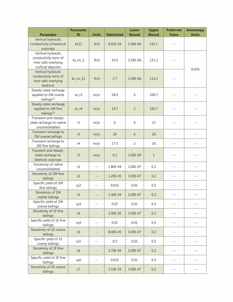
Parameter Parameter

ID Units Optimized Lower Bound

Upper Bound

Preferred Value

Anisotropy Ratio

Vertical hydraulic conductivity of bedrock

outcrops kz12 ft/d 6.02E-04 1.40E-04 141.1 --

Vertical hydraulic conductivity term of river cells overlying

surficial deposits

kz_riv_1 ft/d 35.6 3.28E-06 131.2 --

0.076 Vertical hydraulic

conductivity term of river cells overlying

bedrock

kz_riv_12 ft/d 2.7 3.28E-06 131.2 --

Steady-state recharge applied to 2W coarse

tailings(1) ss_r3 in/yr 28.4 6 100.7 -- --

Steady-state recharge applied to 2W fine

tailings(1) ss_r4 in/yr 19.7 2 100.7 -- --

Transient and steady-state recharge to native

unconsolidated r1 in/yr 6 6 12 -- --

Transient recharge to 2W coarse tailings

r3 in/yr 18 6 18 -- --

Transient recharge to 2W fine tailings

r4 in/yr 17.5 2 18 -- --

Transient and steady-state recharge to bedrock outcrops

r5 in/yr 0.2 1.00E-04 1 -- --

Storativity of native unconsolidated

s1 -- 1.80E-04 1.00E-07 0.2 -- --

Storativity of 2W fine tailings

s2 -- 1.20E-05 1.00E-07 0.2 -- --

Specific yield of 2W fine tailings

sy2 -- 0.033 0.01 0.3 -- --

Storativity of 2W coarse tailings

s3 -- 1.30E-04 1.00E-07 0.2 -- --

Specific yield of 2W coarse tailings

sy3 -- 0.07 0.01 0.3 -- --

Storativity of 1E fine tailings

s4 -- 2.00E-05 1.00E-07 0.2 -- --

Specific yield of 1E fine tailings

sy4 -- 0.01 0.01 0.3 -- --

Storativity of 1E coarse tailings

s5 -- 8.40E-05 1.00E-07 0.2 -- --

Specific yield of 1E coarse tailings

sy5 -- 0.3 0.01 0.3 -- --

Storativity of 2E fine tailings

s6 -- 3.70E-04 1.00E-07 0.2 -- --

Specific yield of 2E fine tailings

sy6 -- 0.015 0.01 0.3 -- --

Storativity of 2E coarse tailings

s7 -- 1.10E-03 1.00E-07 0.2 -- --

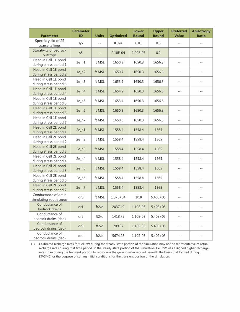
Parameter Parameter

ID Units Optimized Lower Bound

Upper Bound

Preferred Value

Anisotropy Ratio

Specific yield of 2E coarse tailings

sy7 -- 0.024 0.01 0.3 -- --

Storativity of bedrock outcrops

s8 -- 2.10E-04 1.00E-07 0.2 -- --

Head in Cell 1E pond during stress period 1

1e_h1 ft MSL 1650.3 1650.3 1656.8 -- --

Head in Cell 1E pond during stress period 2

1e_h2 ft MSL 1650.7 1650.3 1656.8 -- --

Head in Cell 1E pond during stress period 3

1e_h3 ft MSL 1653.9 1650.3 1656.8 -- --

Head in Cell 1E pond during stress period 4

1e_h4 ft MSL 1654.2 1650.3 1656.8 -- --

Head in Cell 1E pond during stress period 5

1e_h5 ft MSL 1653.4 1650.3 1656.8 -- --

Head in Cell 1E pond during stress period 6

1e_h6 ft MSL 1650.3 1650.3 1656.8 -- --

Head in Cell 1E pond during stress period 7

1e_h7 ft MSL 1650.3 1650.3 1656.8 -- --

Head in Cell 2E pond during stress period 1

2e_h1 ft MSL 1558.4 1558.4 1565 -- --

Head in Cell 2E pond during stress period 2

2e_h2 ft MSL 1558.4 1558.4 1565 -- --

Head in Cell 2E pond during stress period 3

2e_h3 ft MSL 1558.4 1558.4 1565 -- --

Head in Cell 2E pond during stress period 4

2e_h4 ft MSL 1558.4 1558.4 1565 -- --

Head in Cell 2E pond during stress period 5

2e_h5 ft MSL 1558.4 1558.4 1565 -- --

Head in Cell 2E pond during stress period 6

2e_h6 ft MSL 1558.4 1558.4 1565 -- --

Head in Cell 2E pond during stress period 7

2e_h7 ft MSL 1558.4 1558.4 1565 -- --

Conductance of drain simulating south seeps

dr0 ft MSL 1.07E+04 10.8 5.40E+05 -- --

Conductance of bedrock drains

dr1 ft2/d 2837.49 1.10E-03 5.40E+05 -- --

Conductance of bedrock drains (tied)

dr2 ft2/d 1418.75 1.10E-03 5.40E+05 -- --

Conductance of bedrock drains (tied)

dr3 ft2/d 709.37 1.10E-03 5.40E+05 -- --

Conductance of bedrock drains (tied)

dr4 ft2/d 5674.98 1.10E-03 5.40E+05 -- --

(1) Calibrated recharge rates for Cell 2W during the steady-state portion of the simulation may not be representative of actual recharge rates during that time period. In the steady-state portion of the simulation, Cell 2W was assigned higher recharge rates than during the transient portion to reproduce the groundwater mound beneath the basin that formed during LTVSMC for the purpose of setting initial conditions for the transient portion of the simulation.

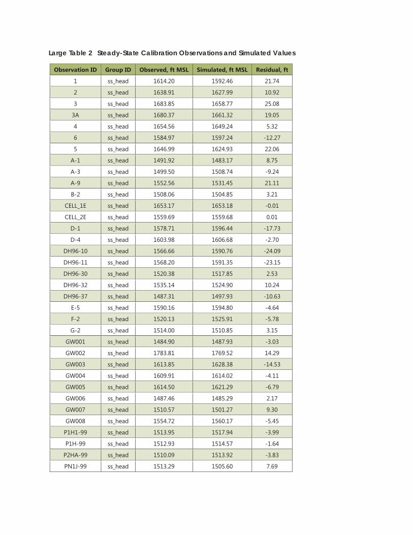
Large Table 2 Steady-State Calibration Observations and Simulated Values

Observation ID Group ID Observed, ft MSL Simulated, ft MSL Residual, ft

1 ss_head 1614.20 1592.46 21.74

2 ss_head 1638.91 1627.99 10.92

3 ss_head 1683.85 1658.77 25.08

3A ss_head 1680.37 1661.32 19.05

4 ss_head 1654.56 1649.24 5.32

6 ss_head 1584.97 1597.24 -12.27

5 ss_head 1646.99 1624.93 22.06

A-1 ss_head 1491.92 1483.17 8.75

A-3 ss_head 1499.50 1508.74 -9.24

A-9 ss_head 1552.56 1531.45 21.11

B-2 ss_head 1508.06 1504.85 3.21

CELL_1E ss_head 1653.17 1653.18 -0.01

CELL_2E ss_head 1559.69 1559.68 0.01

D-1 ss_head 1578.71 1596.44 -17.73

D-4 ss_head 1603.98 1606.68 -2.70

DH96-10 ss_head 1566.66 1590.76 -24.09

DH96-11 ss_head 1568.20 1591.35 -23.15

DH96-30 ss_head 1520.38 1517.85 2.53

DH96-32 ss_head 1535.14 1524.90 10.24

DH96-37 ss_head 1487.31 1497.93 -10.63

E-5 ss_head 1590.16 1594.80 -4.64

F-2 ss_head 1520.13 1525.91 -5.78

G-2 ss_head 1514.00 1510.85 3.15

GW001 ss_head 1484.90 1487.93 -3.03

GW002 ss_head 1783.81 1769.52 14.29

GW003 ss_head 1613.85 1628.38 -14.53

GW004 ss_head 1609.91 1614.02 -4.11

GW005 ss_head 1614.50 1621.29 -6.79

GW006 ss_head 1487.46 1485.29 2.17

GW007 ss_head 1510.57 1501.27 9.30

GW008 ss_head 1554.72 1560.17 -5.45

P1H1-99 ss_head 1513.95 1517.94 -3.99

P1H-99 ss_head 1512.93 1514.57 -1.64

P2HA-99 ss_head 1510.09 1513.92 -3.83

PN1J-99 ss_head 1513.29 1505.60 7.69

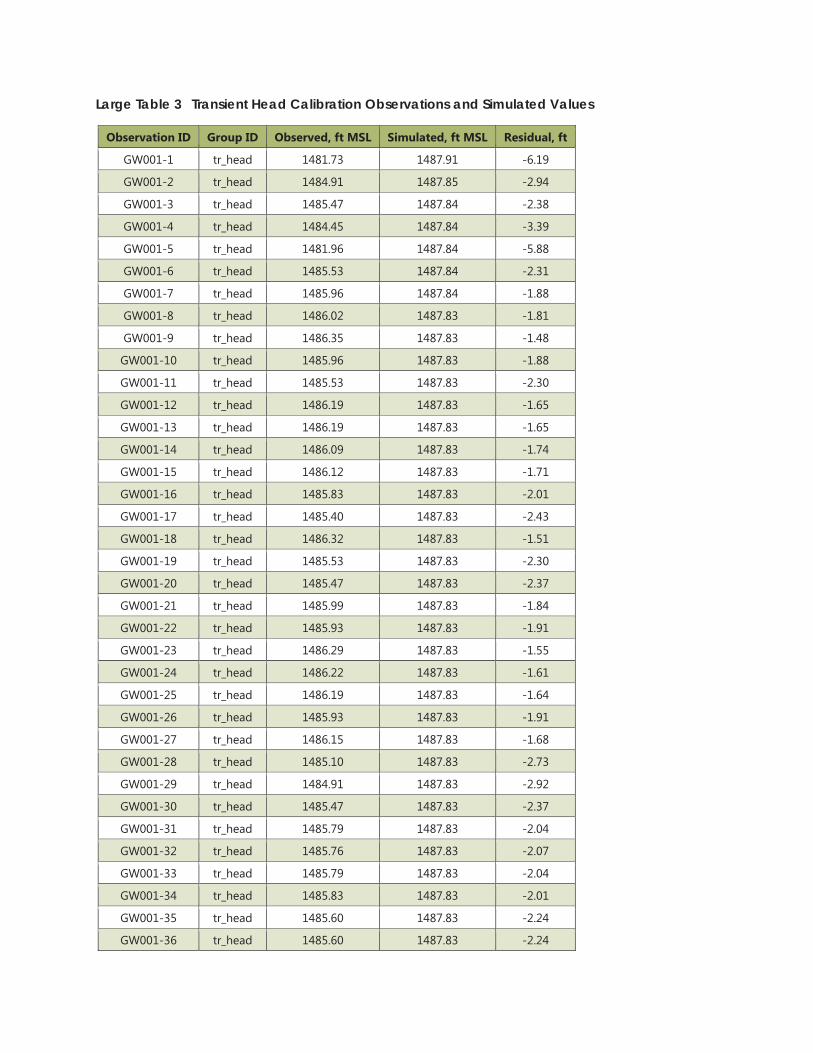
Large Table 3 Transient Head Calibration Observations and Simulated Values

Observation ID Group ID Observed, ft MSL Simulated, ft MSL Residual, ft

GW001-1 tr_head 1481.73 1487.91 -6.19

GW001-2 tr_head 1484.91 1487.85 -2.94

GW001-3 tr_head 1485.47 1487.84 -2.38

GW001-4 tr_head 1484.45 1487.84 -3.39

GW001-5 tr_head 1481.96 1487.84 -5.88

GW001-6 tr_head 1485.53 1487.84 -2.31

GW001-7 tr_head 1485.96 1487.84 -1.88

GW001-8 tr_head 1486.02 1487.83 -1.81

GW001-9 tr_head 1486.35 1487.83 -1.48

GW001-10 tr_head 1485.96 1487.83 -1.88

GW001-11 tr_head 1485.53 1487.83 -2.30

GW001-12 tr_head 1486.19 1487.83 -1.65

GW001-13 tr_head 1486.19 1487.83 -1.65

GW001-14 tr_head 1486.09 1487.83 -1.74

GW001-15 tr_head 1486.12 1487.83 -1.71

GW001-16 tr_head 1485.83 1487.83 -2.01

GW001-17 tr_head 1485.40 1487.83 -2.43

GW001-18 tr_head 1486.32 1487.83 -1.51

GW001-19 tr_head 1485.53 1487.83 -2.30

GW001-20 tr_head 1485.47 1487.83 -2.37

GW001-21 tr_head 1485.99 1487.83 -1.84

GW001-22 tr_head 1485.93 1487.83 -1.91

GW001-23 tr_head 1486.29 1487.83 -1.55

GW001-24 tr_head 1486.22 1487.83 -1.61

GW001-25 tr_head 1486.19 1487.83 -1.64

GW001-26 tr_head 1485.93 1487.83 -1.91

GW001-27 tr_head 1486.15 1487.83 -1.68

GW001-28 tr_head 1485.10 1487.83 -2.73

GW001-29 tr_head 1484.91 1487.83 -2.92

GW001-30 tr_head 1485.47 1487.83 -2.37

GW001-31 tr_head 1485.79 1487.83 -2.04

GW001-32 tr_head 1485.76 1487.83 -2.07

GW001-33 tr_head 1485.79 1487.83 -2.04

GW001-34 tr_head 1485.83 1487.83 -2.01

GW001-35 tr_head 1485.60 1487.83 -2.24

GW001-36 tr_head 1485.60 1487.83 -2.24

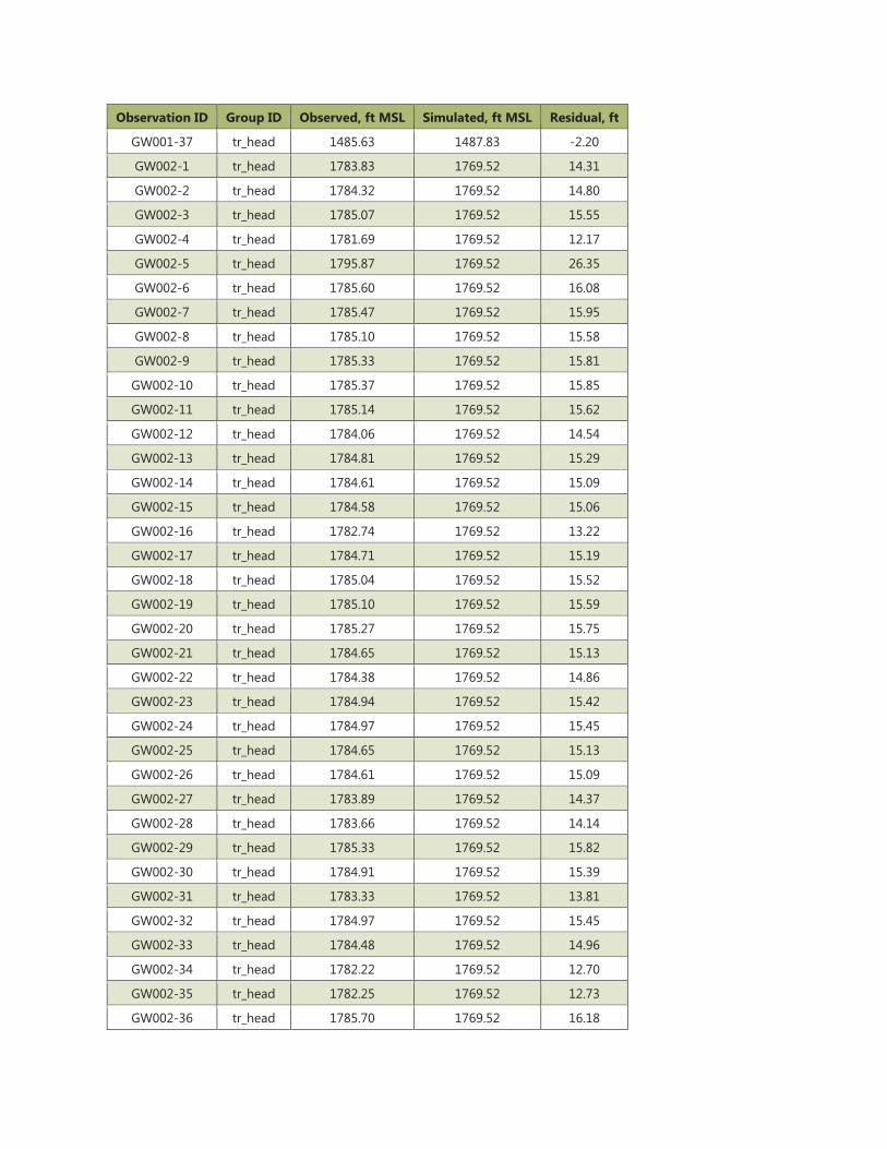
Observation ID Group ID Observed, ft MSL Simulated, ft MSL Residual, ft

GW001-37 tr_head 1485.63 1487.83 -2.20

GW002-1 tr_head 1783.83 1769.52 14.31

GW002-2 tr_head 1784.32 1769.52 14.80

GW002-3 tr_head 1785.07 1769.52 15.55

GW002-4 tr_head 1781.69 1769.52 12.17

GW002-5 tr_head 1795.87 1769.52 26.35

GW002-6 tr_head 1785.60 1769.52 16.08

GW002-7 tr_head 1785.47 1769.52 15.95

GW002-8 tr_head 1785.10 1769.52 15.58

GW002-9 tr_head 1785.33 1769.52 15.81

GW002-10 tr_head 1785.37 1769.52 15.85

GW002-11 tr_head 1785.14 1769.52 15.62

GW002-12 tr_head 1784.06 1769.52 14.54

GW002-13 tr_head 1784.81 1769.52 15.29

GW002-14 tr_head 1784.61 1769.52 15.09

GW002-15 tr_head 1784.58 1769.52 15.06

GW002-16 tr_head 1782.74 1769.52 13.22

GW002-17 tr_head 1784.71 1769.52 15.19

GW002-18 tr_head 1785.04 1769.52 15.52

GW002-19 tr_head 1785.10 1769.52 15.59

GW002-20 tr_head 1785.27 1769.52 15.75

GW002-21 tr_head 1784.65 1769.52 15.13

GW002-22 tr_head 1784.38 1769.52 14.86

GW002-23 tr_head 1784.94 1769.52 15.42

GW002-24 tr_head 1784.97 1769.52 15.45

GW002-25 tr_head 1784.65 1769.52 15.13

GW002-26 tr_head 1784.61 1769.52 15.09

GW002-27 tr_head 1783.89 1769.52 14.37

GW002-28 tr_head 1783.66 1769.52 14.14

GW002-29 tr_head 1785.33 1769.52 15.82

GW002-30 tr_head 1784.91 1769.52 15.39

GW002-31 tr_head 1783.33 1769.52 13.81

GW002-32 tr_head 1784.97 1769.52 15.45

GW002-33 tr_head 1784.48 1769.52 14.96

GW002-34 tr_head 1782.22 1769.52 12.70

GW002-35 tr_head 1782.25 1769.52 12.73

GW002-36 tr_head 1785.70 1769.52 16.18

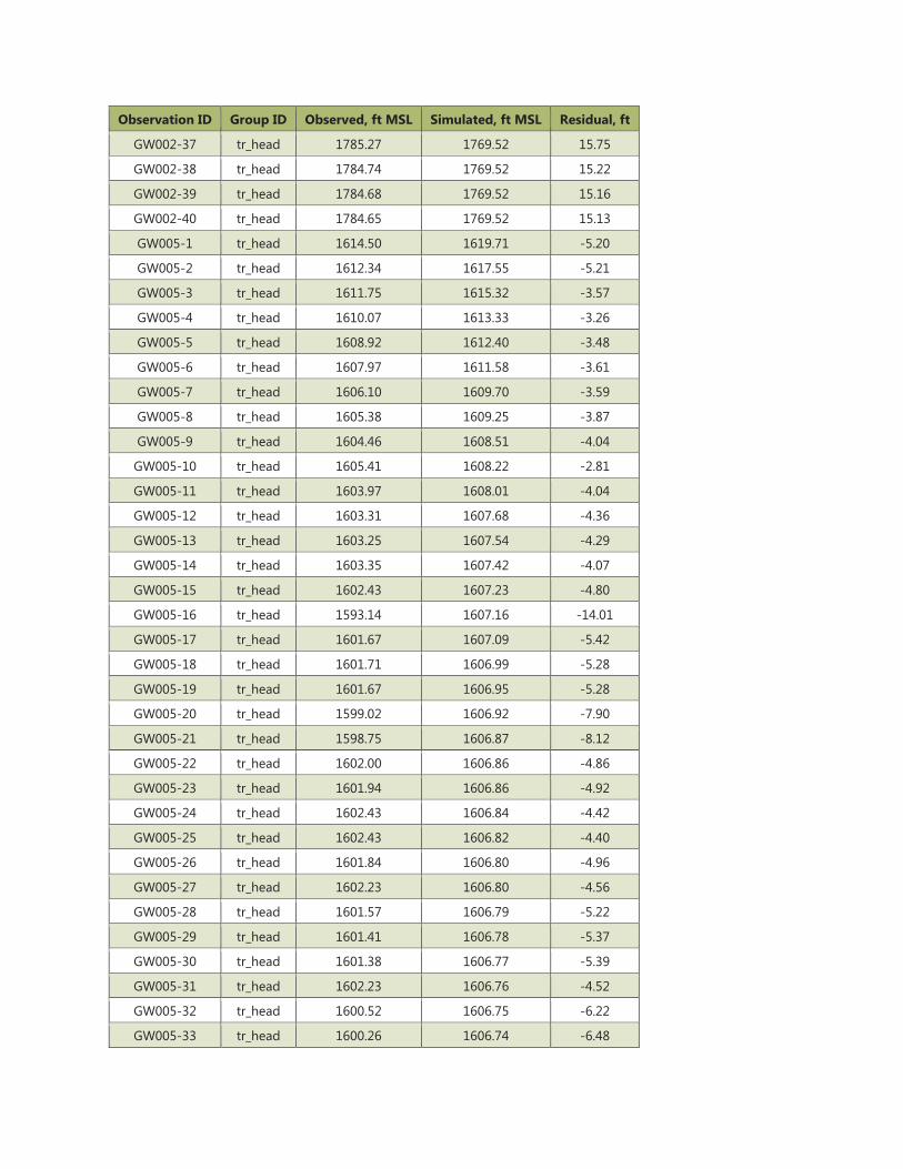
Observation ID Group ID Observed, ft MSL Simulated, ft MSL Residual, ft

GW002-37 tr_head 1785.27 1769.52 15.75

GW002-38 tr_head 1784.74 1769.52 15.22

GW002-39 tr_head 1784.68 1769.52 15.16

GW002-40 tr_head 1784.65 1769.52 15.13

GW005-1 tr_head 1614.50 1619.71 -5.20

GW005-2 tr_head 1612.34 1617.55 -5.21

GW005-3 tr_head 1611.75 1615.32 -3.57

GW005-4 tr_head 1610.07 1613.33 -3.26

GW005-5 tr_head 1608.92 1612.40 -3.48

GW005-6 tr_head 1607.97 1611.58 -3.61

GW005-7 tr_head 1606.10 1609.70 -3.59

GW005-8 tr_head 1605.38 1609.25 -3.87

GW005-9 tr_head 1604.46 1608.51 -4.04

GW005-10 tr_head 1605.41 1608.22 -2.81

GW005-11 tr_head 1603.97 1608.01 -4.04

GW005-12 tr_head 1603.31 1607.68 -4.36

GW005-13 tr_head 1603.25 1607.54 -4.29

GW005-14 tr_head 1603.35 1607.42 -4.07

GW005-15 tr_head 1602.43 1607.23 -4.80

GW005-16 tr_head 1593.14 1607.16 -14.01

GW005-17 tr_head 1601.67 1607.09 -5.42

GW005-18 tr_head 1601.71 1606.99 -5.28

GW005-19 tr_head 1601.67 1606.95 -5.28

GW005-20 tr_head 1599.02 1606.92 -7.90

GW005-21 tr_head 1598.75 1606.87 -8.12

GW005-22 tr_head 1602.00 1606.86 -4.86

GW005-23 tr_head 1601.94 1606.86 -4.92

GW005-24 tr_head 1602.43 1606.84 -4.42

GW005-25 tr_head 1602.43 1606.82 -4.40

GW005-26 tr_head 1601.84 1606.80 -4.96

GW005-27 tr_head 1602.23 1606.80 -4.56

GW005-28 tr_head 1601.57 1606.79 -5.22

GW005-29 tr_head 1601.41 1606.78 -5.37

GW005-30 tr_head 1601.38 1606.77 -5.39

GW005-31 tr_head 1602.23 1606.76 -4.52

GW005-32 tr_head 1600.52 1606.75 -6.22

GW005-33 tr_head 1600.26 1606.74 -6.48

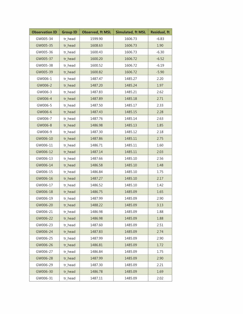
Observation ID Group ID Observed, ft MSL Simulated, ft MSL Residual, ft

GW005-34 tr_head 1599.90 1606.73 -6.83

GW005-35 tr_head 1608.63 1606.73 1.90

GW005-36 tr_head 1600.43 1606.73 -6.30

GW005-37 tr_head 1600.20 1606.72 -6.52

GW005-38 tr_head 1600.52 1606.72 -6.19

GW005-39 tr_head 1600.82 1606.72 -5.90

GW006-1 tr_head 1487.47 1485.27 2.20

GW006-2 tr_head 1487.20 1485.24 1.97

GW006-3 tr_head 1487.83 1485.21 2.62

GW006-4 tr_head 1487.89 1485.18 2.71

GW006-5 tr_head 1487.50 1485.17 2.33

GW006-6 tr_head 1487.43 1485.15 2.28

GW006-7 tr_head 1487.76 1485.14 2.63

GW006-8 tr_head 1486.98 1485.13 1.85

GW006-9 tr_head 1487.30 1485.12 2.18

GW006-10 tr_head 1487.86 1485.11 2.75

GW006-11 tr_head 1486.71 1485.11 1.60

GW006-12 tr_head 1487.14 1485.11 2.03

GW006-13 tr_head 1487.66 1485.10 2.56

GW006-14 tr_head 1486.58 1485.10 1.48

GW006-15 tr_head 1486.84 1485.10 1.75

GW006-16 tr_head 1487.27 1485.10 2.17

GW006-17 tr_head 1486.52 1485.10 1.42

GW006-18 tr_head 1486.75 1485.09 1.65

GW006-19 tr_head 1487.99 1485.09 2.90

GW006-20 tr_head 1488.22 1485.09 3.13

GW006-21 tr_head 1486.98 1485.09 1.88

GW006-22 tr_head 1486.98 1485.09 1.88

GW006-23 tr_head 1487.60 1485.09 2.51

GW006-24 tr_head 1487.83 1485.09 2.74

GW006-25 tr_head 1487.99 1485.09 2.90

GW006-26 tr_head 1486.81 1485.09 1.72

GW006-27 tr_head 1486.84 1485.09 1.75

GW006-28 tr_head 1487.99 1485.09 2.90

GW006-29 tr_head 1487.30 1485.09 2.21

GW006-30 tr_head 1486.78 1485.09 1.69

GW006-31 tr_head 1487.11 1485.09 2.02

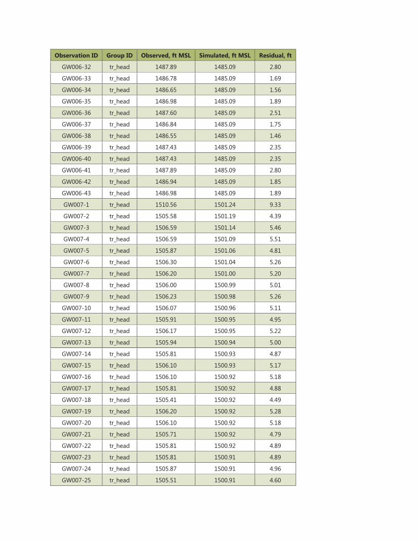
Observation ID Group ID Observed, ft MSL Simulated, ft MSL Residual, ft

GW006-32 tr_head 1487.89 1485.09 2.80

GW006-33 tr_head 1486.78 1485.09 1.69

GW006-34 tr_head 1486.65 1485.09 1.56

GW006-35 tr_head 1486.98 1485.09 1.89

GW006-36 tr_head 1487.60 1485.09 2.51

GW006-37 tr_head 1486.84 1485.09 1.75

GW006-38 tr_head 1486.55 1485.09 1.46

GW006-39 tr_head 1487.43 1485.09 2.35

GW006-40 tr_head 1487.43 1485.09 2.35

GW006-41 tr_head 1487.89 1485.09 2.80

GW006-42 tr_head 1486.94 1485.09 1.85

GW006-43 tr_head 1486.98 1485.09 1.89

GW007-1 tr_head 1510.56 1501.24 9.33

GW007-2 tr_head 1505.58 1501.19 4.39

GW007-3 tr_head 1506.59 1501.14 5.46

GW007-4 tr_head 1506.59 1501.09 5.51

GW007-5 tr_head 1505.87 1501.06 4.81

GW007-6 tr_head 1506.30 1501.04 5.26

GW007-7 tr_head 1506.20 1501.00 5.20

GW007-8 tr_head 1506.00 1500.99 5.01

GW007-9 tr_head 1506.23 1500.98 5.26

GW007-10 tr_head 1506.07 1500.96 5.11

GW007-11 tr_head 1505.91 1500.95 4.95

GW007-12 tr_head 1506.17 1500.95 5.22

GW007-13 tr_head 1505.94 1500.94 5.00

GW007-14 tr_head 1505.81 1500.93 4.87

GW007-15 tr_head 1506.10 1500.93 5.17

GW007-16 tr_head 1506.10 1500.92 5.18

GW007-17 tr_head 1505.81 1500.92 4.88

GW007-18 tr_head 1505.41 1500.92 4.49

GW007-19 tr_head 1506.20 1500.92 5.28

GW007-20 tr_head 1506.10 1500.92 5.18

GW007-21 tr_head 1505.71 1500.92 4.79

GW007-22 tr_head 1505.81 1500.92 4.89

GW007-23 tr_head 1505.81 1500.91 4.89

GW007-24 tr_head 1505.87 1500.91 4.96

GW007-25 tr_head 1505.51 1500.91 4.60

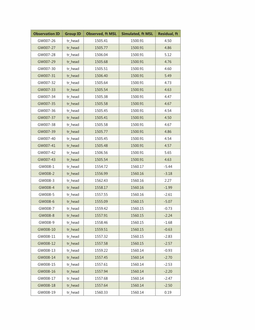
Observation ID Group ID Observed, ft MSL Simulated, ft MSL Residual, ft

GW007-26 tr_head 1505.41 1500.91 4.50

GW007-27 tr_head 1505.77 1500.91 4.86

GW007-28 tr_head 1506.04 1500.91 5.12

GW007-29 tr_head 1505.68 1500.91 4.76

GW007-30 tr_head 1505.51 1500.91 4.60

GW007-31 tr_head 1506.40 1500.91 5.49

GW007-32 tr_head 1505.64 1500.91 4.73

GW007-33 tr_head 1505.54 1500.91 4.63

GW007-34 tr_head 1505.38 1500.91 4.47

GW007-35 tr_head 1505.58 1500.91 4.67

GW007-36 tr_head 1505.45 1500.91 4.54

GW007-37 tr_head 1505.41 1500.91 4.50

GW007-38 tr_head 1505.58 1500.91 4.67

GW007-39 tr_head 1505.77 1500.91 4.86

GW007-40 tr_head 1505.45 1500.91 4.54

GW007-41 tr_head 1505.48 1500.91 4.57

GW007-42 tr_head 1506.56 1500.91 5.65

GW007-43 tr_head 1505.54 1500.91 4.63

GW008-1 tr_head 1554.72 1560.17 -5.44

GW008-2 tr_head 1556.99 1560.16 -3.18

GW008-3 tr_head 1562.43 1560.16 2.27

GW008-4 tr_head 1558.17 1560.16 -1.99

GW008-5 tr_head 1557.55 1560.16 -2.61

GW008-6 tr_head 1555.09 1560.15 -5.07

GW008-7 tr_head 1559.42 1560.15 -0.73

GW008-8 tr_head 1557.91 1560.15 -2.24

GW008-9 tr_head 1558.46 1560.15 -1.68

GW008-10 tr_head 1559.51 1560.15 -0.63

GW008-11 tr_head 1557.32 1560.15 -2.83

GW008-12 tr_head 1557.58 1560.15 -2.57

GW008-13 tr_head 1559.22 1560.14 -0.93

GW008-14 tr_head 1557.45 1560.14 -2.70

GW008-15 tr_head 1557.61 1560.14 -2.53

GW008-16 tr_head 1557.94 1560.14 -2.20

GW008-17 tr_head 1557.68 1560.14 -2.47

GW008-18 tr_head 1557.64 1560.14 -2.50

GW008-19 tr_head 1560.33 1560.14 0.19

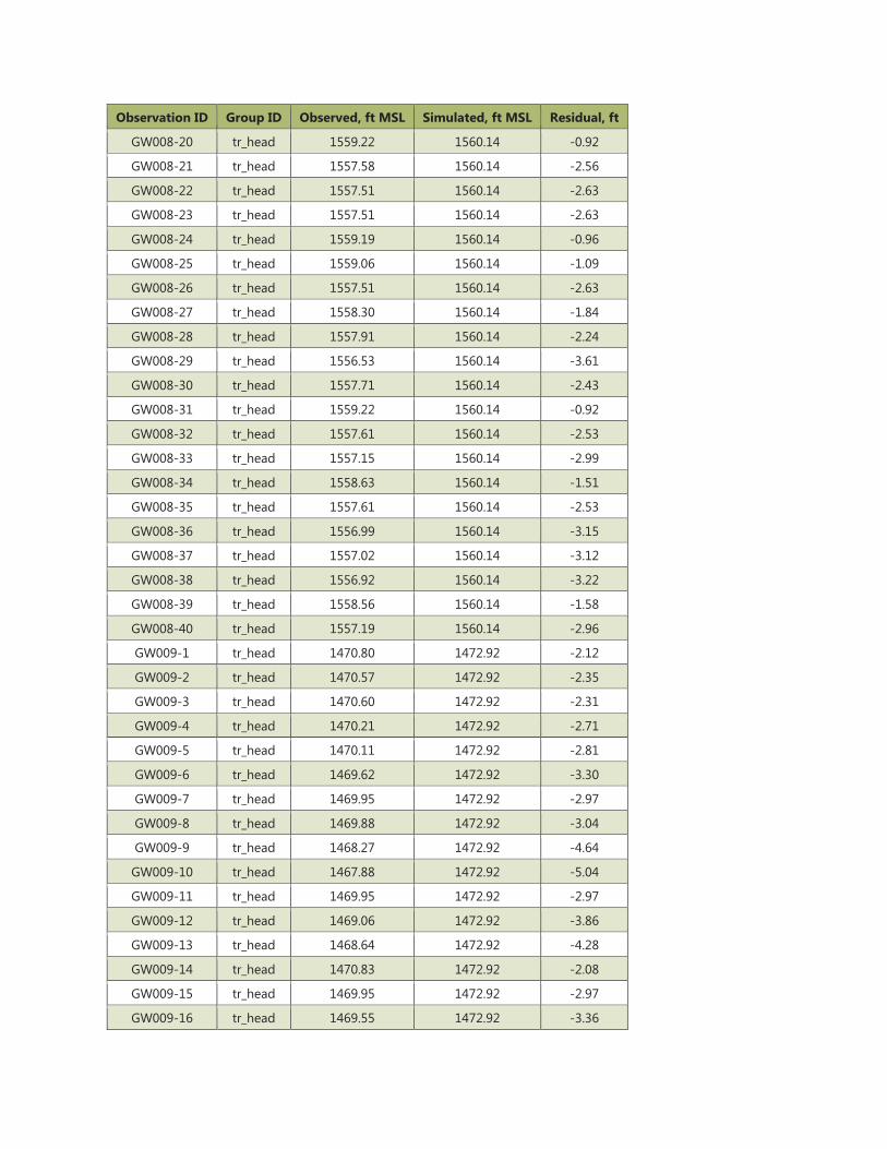
Observation ID Group ID Observed, ft MSL Simulated, ft MSL Residual, ft

GW008-20 tr_head 1559.22 1560.14 -0.92

GW008-21 tr_head 1557.58 1560.14 -2.56

GW008-22 tr_head 1557.51 1560.14 -2.63

GW008-23 tr_head 1557.51 1560.14 -2.63

GW008-24 tr_head 1559.19 1560.14 -0.96

GW008-25 tr_head 1559.06 1560.14 -1.09

GW008-26 tr_head 1557.51 1560.14 -2.63

GW008-27 tr_head 1558.30 1560.14 -1.84

GW008-28 tr_head 1557.91 1560.14 -2.24

GW008-29 tr_head 1556.53 1560.14 -3.61

GW008-30 tr_head 1557.71 1560.14 -2.43

GW008-31 tr_head 1559.22 1560.14 -0.92

GW008-32 tr_head 1557.61 1560.14 -2.53

GW008-33 tr_head 1557.15 1560.14 -2.99

GW008-34 tr_head 1558.63 1560.14 -1.51

GW008-35 tr_head 1557.61 1560.14 -2.53

GW008-36 tr_head 1556.99 1560.14 -3.15

GW008-37 tr_head 1557.02 1560.14 -3.12

GW008-38 tr_head 1556.92 1560.14 -3.22

GW008-39 tr_head 1558.56 1560.14 -1.58

GW008-40 tr_head 1557.19 1560.14 -2.96

GW009-1 tr_head 1470.80 1472.92 -2.12

GW009-2 tr_head 1470.57 1472.92 -2.35

GW009-3 tr_head 1470.60 1472.92 -2.31

GW009-4 tr_head 1470.21 1472.92 -2.71

GW009-5 tr_head 1470.11 1472.92 -2.81

GW009-6 tr_head 1469.62 1472.92 -3.30

GW009-7 tr_head 1469.95 1472.92 -2.97

GW009-8 tr_head 1469.88 1472.92 -3.04

GW009-9 tr_head 1468.27 1472.92 -4.64

GW009-10 tr_head 1467.88 1472.92 -5.04

GW009-11 tr_head 1469.95 1472.92 -2.97

GW009-12 tr_head 1469.06 1472.92 -3.86

GW009-13 tr_head 1468.64 1472.92 -4.28

GW009-14 tr_head 1470.83 1472.92 -2.08

GW009-15 tr_head 1469.95 1472.92 -2.97

GW009-16 tr_head 1469.55 1472.92 -3.36

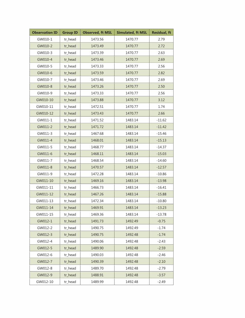
Observation ID Group ID Observed, ft MSL Simulated, ft MSL Residual, ft

GW010-1 tr_head 1473.56 1470.77 2.79

GW010-2 tr_head 1473.49 1470.77 2.72

GW010-3 tr_head 1473.39 1470.77 2.63

GW010-4 tr_head 1473.46 1470.77 2.69

GW010-5 tr_head 1473.33 1470.77 2.56

GW010-6 tr_head 1473.59 1470.77 2.82

GW010-7 tr_head 1473.46 1470.77 2.69

GW010-8 tr_head 1473.26 1470.77 2.50

GW010-9 tr_head 1473.33 1470.77 2.56

GW010-10 tr_head 1473.88 1470.77 3.12

GW010-11 tr_head 1472.51 1470.77 1.74

GW010-12 tr_head 1473.43 1470.77 2.66

GW011-1 tr_head 1471.52 1483.14 -11.62

GW011-2 tr_head 1471.72 1483.14 -11.42

GW011-3 tr_head 1467.68 1483.14 -15.46

GW011-4 tr_head 1468.01 1483.14 -15.13

GW011-5 tr_head 1468.77 1483.14 -14.37

GW011-6 tr_head 1468.11 1483.14 -15.03

GW011-7 tr_head 1468.54 1483.14 -14.60

GW011-8 tr_head 1470.57 1483.14 -12.57

GW011-9 tr_head 1472.28 1483.14 -10.86

GW011-10 tr_head 1469.16 1483.14 -13.98

GW011-11 tr_head 1466.73 1483.14 -16.41

GW011-12 tr_head 1467.26 1483.14 -15.88

GW011-13 tr_head 1472.34 1483.14 -10.80

GW011-14 tr_head 1469.91 1483.14 -13.23

GW011-15 tr_head 1469.36 1483.14 -13.78

GW012-1 tr_head 1491.73 1492.49 -0.75

GW012-2 tr_head 1490.75 1492.49 -1.74

GW012-3 tr_head 1490.75 1492.48 -1.74

GW012-4 tr_head 1490.06 1492.48 -2.43

GW012-5 tr_head 1489.90 1492.48 -2.59

GW012-6 tr_head 1490.03 1492.48 -2.46

GW012-7 tr_head 1490.39 1492.48 -2.10

GW012-8 tr_head 1489.70 1492.48 -2.79

GW012-9 tr_head 1488.91 1492.48 -3.57

GW012-10 tr_head 1489.99 1492.48 -2.49

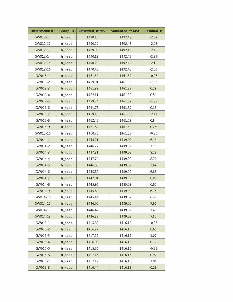
Observation ID Group ID Observed, ft MSL Simulated, ft MSL Residual, ft

GW012-11 tr_head 1490.16 1492.48 -2.33

GW012-12 tr_head 1490.22 1492.48 -2.26

GW012-13 tr_head 1489.99 1492.48 -2.49

GW012-14 tr_head 1490.19 1492.48 -2.29

GW012-15 tr_head 1490.29 1492.48 -2.19

GW012-16 tr_head 1490.45 1492.48 -2.03

GW013-1 tr_head 1461.52 1461.59 -0.08

GW013-2 tr_head 1459.91 1461.59 -1.68

GW013-3 tr_head 1461.88 1461.59 0.28

GW013-4 tr_head 1462.11 1461.59 0.51

GW013-5 tr_head 1459.74 1461.59 -1.85

GW013-6 tr_head 1461.75 1461.59 0.15

GW013-7 tr_head 1459.19 1461.59 -2.41

GW013-8 tr_head 1462.43 1461.59 0.84

GW013-9 tr_head 1461.84 1461.59 0.25

GW013-10 tr_head 1460.70 1461.59 -0.90

GW014-1 tr_head 1445.21 1439.02 6.19

GW014-2 tr_head 1446.72 1439.02 7.70

GW014-3 tr_head 1447.31 1439.02 8.29

GW014-4 tr_head 1447.74 1439.02 8.72

GW014-5 tr_head 1446.65 1439.02 7.64

GW014-6 tr_head 1445.87 1439.02 6.85

GW014-7 tr_head 1447.01 1439.02 8.00

GW014-8 tr_head 1445.96 1439.02 6.95

GW014-9 tr_head 1445.80 1439.02 6.78

GW014-10 tr_head 1445.44 1439.02 6.42

GW014-11 tr_head 1446.92 1439.02 7.90

GW014-12 tr_head 1446.42 1439.02 7.41

GW014-13 tr_head 1446.59 1439.02 7.57

GW015-1 tr_head 1415.88 1416.15 -0.27

GW015-2 tr_head 1416.77 1416.15 0.61

GW015-3 tr_head 1417.22 1416.15 1.07

GW015-4 tr_head 1416.93 1416.15 0.77

GW015-5 tr_head 1415.85 1416.15 -0.31

GW015-6 tr_head 1417.13 1416.15 0.97

GW015-7 tr_head 1417.19 1416.15 1.04

GW015-8 tr_head 1416.44 1416.15 0.28

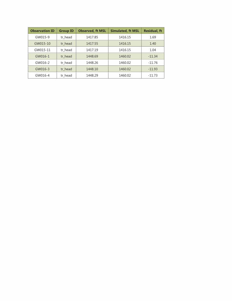
Observation ID Group ID Observed, ft MSL Simulated, ft MSL Residual, ft

GW015-9 tr_head 1417.85 1416.15 1.69

GW015-10 tr_head 1417.55 1416.15 1.40

GW015-11 tr_head 1417.19 1416.15 1.04

GW016-1 tr_head 1448.69 1460.02 -11.34

GW016-2 tr_head 1448.26 1460.02 -11.76

GW016-3 tr_head 1448.10 1460.02 -11.93

GW016-4 tr_head 1448.29 1460.02 -11.73

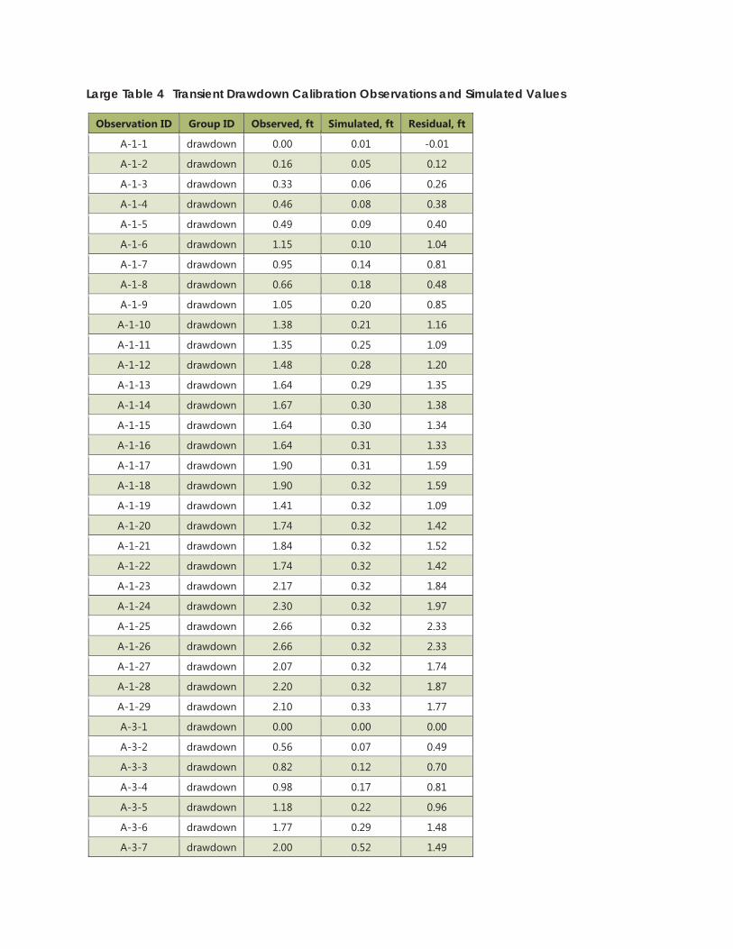
Large Table 4 Transient Drawdown Calibration Observations and Simulated Values

Observation ID Group ID Observed, ft Simulated, ft Residual, ft

A-1-1 drawdown 0.00 0.01 -0.01

A-1-2 drawdown 0.16 0.05 0.12

A-1-3 drawdown 0.33 0.06 0.26

A-1-4 drawdown 0.46 0.08 0.38

A-1-5 drawdown 0.49 0.09 0.40

A-1-6 drawdown 1.15 0.10 1.04

A-1-7 drawdown 0.95 0.14 0.81

A-1-8 drawdown 0.66 0.18 0.48

A-1-9 drawdown 1.05 0.20 0.85

A-1-10 drawdown 1.38 0.21 1.16

A-1-11 drawdown 1.35 0.25 1.09

A-1-12 drawdown 1.48 0.28 1.20

A-1-13 drawdown 1.64 0.29 1.35

A-1-14 drawdown 1.67 0.30 1.38

A-1-15 drawdown 1.64 0.30 1.34

A-1-16 drawdown 1.64 0.31 1.33

A-1-17 drawdown 1.90 0.31 1.59

A-1-18 drawdown 1.90 0.32 1.59

A-1-19 drawdown 1.41 0.32 1.09

A-1-20 drawdown 1.74 0.32 1.42

A-1-21 drawdown 1.84 0.32 1.52

A-1-22 drawdown 1.74 0.32 1.42

A-1-23 drawdown 2.17 0.32 1.84

A-1-24 drawdown 2.30 0.32 1.97

A-1-25 drawdown 2.66 0.32 2.33

A-1-26 drawdown 2.66 0.32 2.33

A-1-27 drawdown 2.07 0.32 1.74

A-1-28 drawdown 2.20 0.32 1.87

A-1-29 drawdown 2.10 0.33 1.77

A-3-1 drawdown 0.00 0.00 0.00

A-3-2 drawdown 0.56 0.07 0.49

A-3-3 drawdown 0.82 0.12 0.70

A-3-4 drawdown 0.98 0.17 0.81

A-3-5 drawdown 1.18 0.22 0.96

A-3-6 drawdown 1.77 0.29 1.48

A-3-7 drawdown 2.00 0.52 1.49

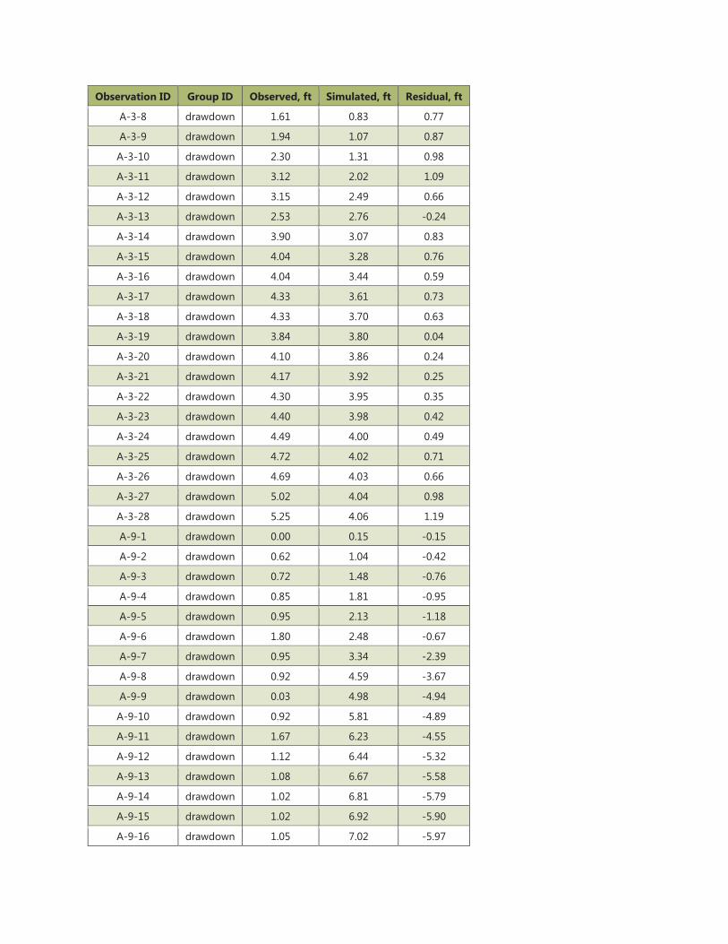
Observation ID Group ID Observed, ft Simulated, ft Residual, ft

A-3-8 drawdown 1.61 0.83 0.77

A-3-9 drawdown 1.94 1.07 0.87

A-3-10 drawdown 2.30 1.31 0.98

A-3-11 drawdown 3.12 2.02 1.09

A-3-12 drawdown 3.15 2.49 0.66

A-3-13 drawdown 2.53 2.76 -0.24

A-3-14 drawdown 3.90 3.07 0.83

A-3-15 drawdown 4.04 3.28 0.76

A-3-16 drawdown 4.04 3.44 0.59

A-3-17 drawdown 4.33 3.61 0.73

A-3-18 drawdown 4.33 3.70 0.63

A-3-19 drawdown 3.84 3.80 0.04

A-3-20 drawdown 4.10 3.86 0.24

A-3-21 drawdown 4.17 3.92 0.25

A-3-22 drawdown 4.30 3.95 0.35

A-3-23 drawdown 4.40 3.98 0.42

A-3-24 drawdown 4.49 4.00 0.49

A-3-25 drawdown 4.72 4.02 0.71

A-3-26 drawdown 4.69 4.03 0.66

A-3-27 drawdown 5.02 4.04 0.98

A-3-28 drawdown 5.25 4.06 1.19

A-9-1 drawdown 0.00 0.15 -0.15

A-9-2 drawdown 0.62 1.04 -0.42

A-9-3 drawdown 0.72 1.48 -0.76

A-9-4 drawdown 0.85 1.81 -0.95

A-9-5 drawdown 0.95 2.13 -1.18

A-9-6 drawdown 1.80 2.48 -0.67

A-9-7 drawdown 0.95 3.34 -2.39

A-9-8 drawdown 0.92 4.59 -3.67

A-9-9 drawdown 0.03 4.98 -4.94

A-9-10 drawdown 0.92 5.81 -4.89

A-9-11 drawdown 1.67 6.23 -4.55

A-9-12 drawdown 1.12 6.44 -5.32

A-9-13 drawdown 1.08 6.67 -5.58

A-9-14 drawdown 1.02 6.81 -5.79

A-9-15 drawdown 1.02 6.92 -5.90

A-9-16 drawdown 1.05 7.02 -5.97

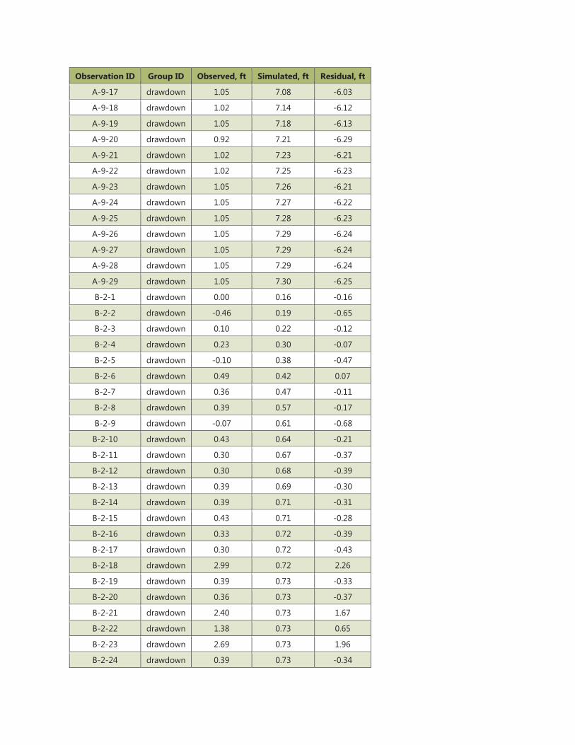
Observation ID Group ID Observed, ft Simulated, ft Residual, ft

A-9-17 drawdown 1.05 7.08 -6.03

A-9-18 drawdown 1.02 7.14 -6.12

A-9-19 drawdown 1.05 7.18 -6.13

A-9-20 drawdown 0.92 7.21 -6.29

A-9-21 drawdown 1.02 7.23 -6.21

A-9-22 drawdown 1.02 7.25 -6.23

A-9-23 drawdown 1.05 7.26 -6.21

A-9-24 drawdown 1.05 7.27 -6.22

A-9-25 drawdown 1.05 7.28 -6.23

A-9-26 drawdown 1.05 7.29 -6.24

A-9-27 drawdown 1.05 7.29 -6.24

A-9-28 drawdown 1.05 7.29 -6.24

A-9-29 drawdown 1.05 7.30 -6.25

B-2-1 drawdown 0.00 0.16 -0.16

B-2-2 drawdown -0.46 0.19 -0.65

B-2-3 drawdown 0.10 0.22 -0.12

B-2-4 drawdown 0.23 0.30 -0.07

B-2-5 drawdown -0.10 0.38 -0.47

B-2-6 drawdown 0.49 0.42 0.07

B-2-7 drawdown 0.36 0.47 -0.11

B-2-8 drawdown 0.39 0.57 -0.17

B-2-9 drawdown -0.07 0.61 -0.68

B-2-10 drawdown 0.43 0.64 -0.21

B-2-11 drawdown 0.30 0.67 -0.37

B-2-12 drawdown 0.30 0.68 -0.39

B-2-13 drawdown 0.39 0.69 -0.30

B-2-14 drawdown 0.39 0.71 -0.31

B-2-15 drawdown 0.43 0.71 -0.28

B-2-16 drawdown 0.33 0.72 -0.39

B-2-17 drawdown 0.30 0.72 -0.43

B-2-18 drawdown 2.99 0.72 2.26

B-2-19 drawdown 0.39 0.73 -0.33

B-2-20 drawdown 0.36 0.73 -0.37

B-2-21 drawdown 2.40 0.73 1.67

B-2-22 drawdown 1.38 0.73 0.65

B-2-23 drawdown 2.69 0.73 1.96

B-2-24 drawdown 0.39 0.73 -0.34

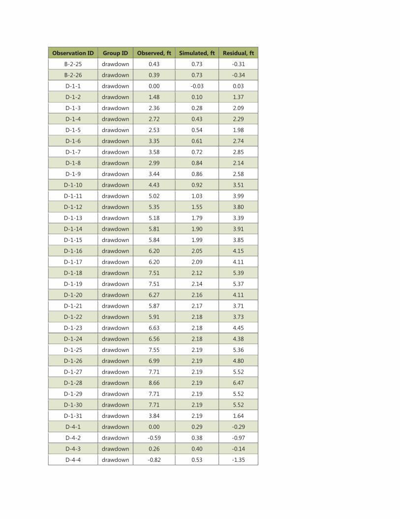
Observation ID Group ID Observed, ft Simulated, ft Residual, ft

B-2-25 drawdown 0.43 0.73 -0.31

B-2-26 drawdown 0.39 0.73 -0.34

D-1-1 drawdown 0.00 -0.03 0.03

D-1-2 drawdown 1.48 0.10 1.37

D-1-3 drawdown 2.36 0.28 2.09

D-1-4 drawdown 2.72 0.43 2.29

D-1-5 drawdown 2.53 0.54 1.98

D-1-6 drawdown 3.35 0.61 2.74

D-1-7 drawdown 3.58 0.72 2.85

D-1-8 drawdown 2.99 0.84 2.14

D-1-9 drawdown 3.44 0.86 2.58

D-1-10 drawdown 4.43 0.92 3.51

D-1-11 drawdown 5.02 1.03 3.99

D-1-12 drawdown 5.35 1.55 3.80

D-1-13 drawdown 5.18 1.79 3.39

D-1-14 drawdown 5.81 1.90 3.91

D-1-15 drawdown 5.84 1.99 3.85

D-1-16 drawdown 6.20 2.05 4.15

D-1-17 drawdown 6.20 2.09 4.11

D-1-18 drawdown 7.51 2.12 5.39

D-1-19 drawdown 7.51 2.14 5.37

D-1-20 drawdown 6.27 2.16 4.11

D-1-21 drawdown 5.87 2.17 3.71

D-1-22 drawdown 5.91 2.18 3.73

D-1-23 drawdown 6.63 2.18 4.45

D-1-24 drawdown 6.56 2.18 4.38

D-1-25 drawdown 7.55 2.19 5.36

D-1-26 drawdown 6.99 2.19 4.80

D-1-27 drawdown 7.71 2.19 5.52

D-1-28 drawdown 8.66 2.19 6.47

D-1-29 drawdown 7.71 2.19 5.52

D-1-30 drawdown 7.71 2.19 5.52

D-1-31 drawdown 3.84 2.19 1.64

D-4-1 drawdown 0.00 0.29 -0.29

D-4-2 drawdown -0.59 0.38 -0.97

D-4-3 drawdown 0.26 0.40 -0.14

D-4-4 drawdown -0.82 0.53 -1.35

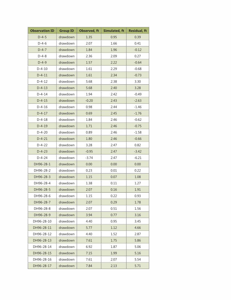
Observation ID Group ID Observed, ft Simulated, ft Residual, ft

D-4-5 drawdown 1.35 0.95 0.39

D-4-6 drawdown 2.07 1.66 0.41

D-4-7 drawdown 1.84 1.96 -0.12

D-4-8 drawdown 2.36 2.09 0.27

D-4-9 drawdown 1.57 2.22 -0.64

D-4-10 drawdown 1.61 2.29 -0.68

D-4-11 drawdown 1.61 2.34 -0.73

D-4-12 drawdown 5.68 2.38 3.30

D-4-13 drawdown 5.68 2.40 3.28

D-4-14 drawdown 1.94 2.42 -0.49

D-4-15 drawdown -0.20 2.43 -2.63

D-4-16 drawdown 0.98 2.44 -1.46

D-4-17 drawdown 0.69 2.45 -1.76

D-4-18 drawdown 1.84 2.46 -0.62

D-4-19 drawdown 1.71 2.46 -0.75

D-4-20 drawdown 0.89 2.46 -1.58

D-4-21 drawdown 1.80 2.46 -0.66

D-4-22 drawdown 3.28 2.47 0.82

D-4-23 drawdown -0.95 2.47 -3.42

D-4-24 drawdown -3.74 2.47 -6.21

DH96-28-1 drawdown 0.00 0.00 0.00

DH96-28-2 drawdown 0.23 0.01 0.22

DH96-28-3 drawdown 1.15 0.07 1.08

DH96-28-4 drawdown 1.38 0.11 1.27

DH96-28-5 drawdown 2.07 0.16 1.91

DH96-28-6 drawdown 1.15 0.22 0.93

DH96-28-7 drawdown 2.07 0.29 1.78

DH96-28-8 drawdown 2.07 0.51 1.56

DH96-28-9 drawdown 3.94 0.77 3.16

DH96-28-10 drawdown 4.40 0.95 3.45

DH96-28-11 drawdown 5.77 1.12 4.66

DH96-28-12 drawdown 4.40 1.52 2.87

DH96-28-13 drawdown 7.61 1.75 5.86

DH96-28-14 drawdown 6.92 1.87 5.06

DH96-28-15 drawdown 7.15 1.99 5.16

DH96-28-16 drawdown 7.61 2.07 5.54

DH96-28-17 drawdown 7.84 2.13 5.71

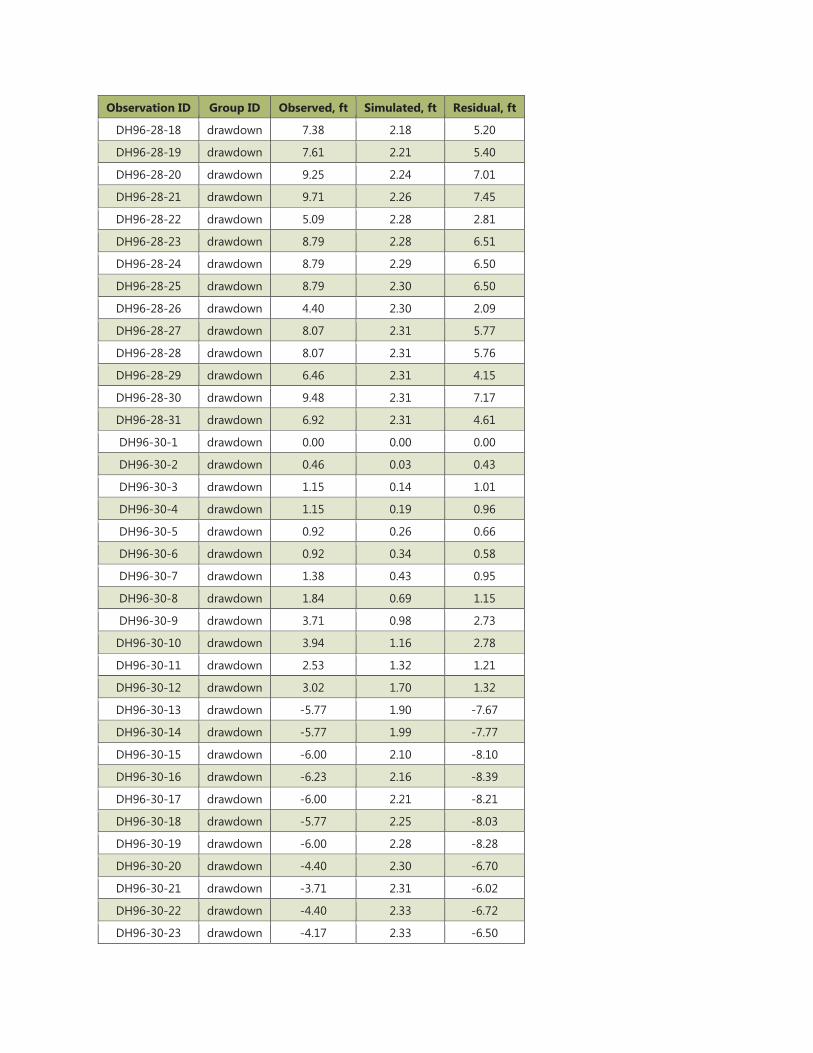
Observation ID Group ID Observed, ft Simulated, ft Residual, ft

DH96-28-18 drawdown 7.38 2.18 5.20

DH96-28-19 drawdown 7.61 2.21 5.40

DH96-28-20 drawdown 9.25 2.24 7.01

DH96-28-21 drawdown 9.71 2.26 7.45

DH96-28-22 drawdown 5.09 2.28 2.81

DH96-28-23 drawdown 8.79 2.28 6.51

DH96-28-24 drawdown 8.79 2.29 6.50

DH96-28-25 drawdown 8.79 2.30 6.50

DH96-28-26 drawdown 4.40 2.30 2.09

DH96-28-27 drawdown 8.07 2.31 5.77

DH96-28-28 drawdown 8.07 2.31 5.76

DH96-28-29 drawdown 6.46 2.31 4.15

DH96-28-30 drawdown 9.48 2.31 7.17

DH96-28-31 drawdown 6.92 2.31 4.61

DH96-30-1 drawdown 0.00 0.00 0.00

DH96-30-2 drawdown 0.46 0.03 0.43

DH96-30-3 drawdown 1.15 0.14 1.01

DH96-30-4 drawdown 1.15 0.19 0.96

DH96-30-5 drawdown 0.92 0.26 0.66

DH96-30-6 drawdown 0.92 0.34 0.58

DH96-30-7 drawdown 1.38 0.43 0.95

DH96-30-8 drawdown 1.84 0.69 1.15

DH96-30-9 drawdown 3.71 0.98 2.73

DH96-30-10 drawdown 3.94 1.16 2.78

DH96-30-11 drawdown 2.53 1.32 1.21

DH96-30-12 drawdown 3.02 1.70 1.32

DH96-30-13 drawdown -5.77 1.90 -7.67

DH96-30-14 drawdown -5.77 1.99 -7.77

DH96-30-15 drawdown -6.00 2.10 -8.10

DH96-30-16 drawdown -6.23 2.16 -8.39

DH96-30-17 drawdown -6.00 2.21 -8.21

DH96-30-18 drawdown -5.77 2.25 -8.03

DH96-30-19 drawdown -6.00 2.28 -8.28

DH96-30-20 drawdown -4.40 2.30 -6.70

DH96-30-21 drawdown -3.71 2.31 -6.02

DH96-30-22 drawdown -4.40 2.33 -6.72

DH96-30-23 drawdown -4.17 2.33 -6.50

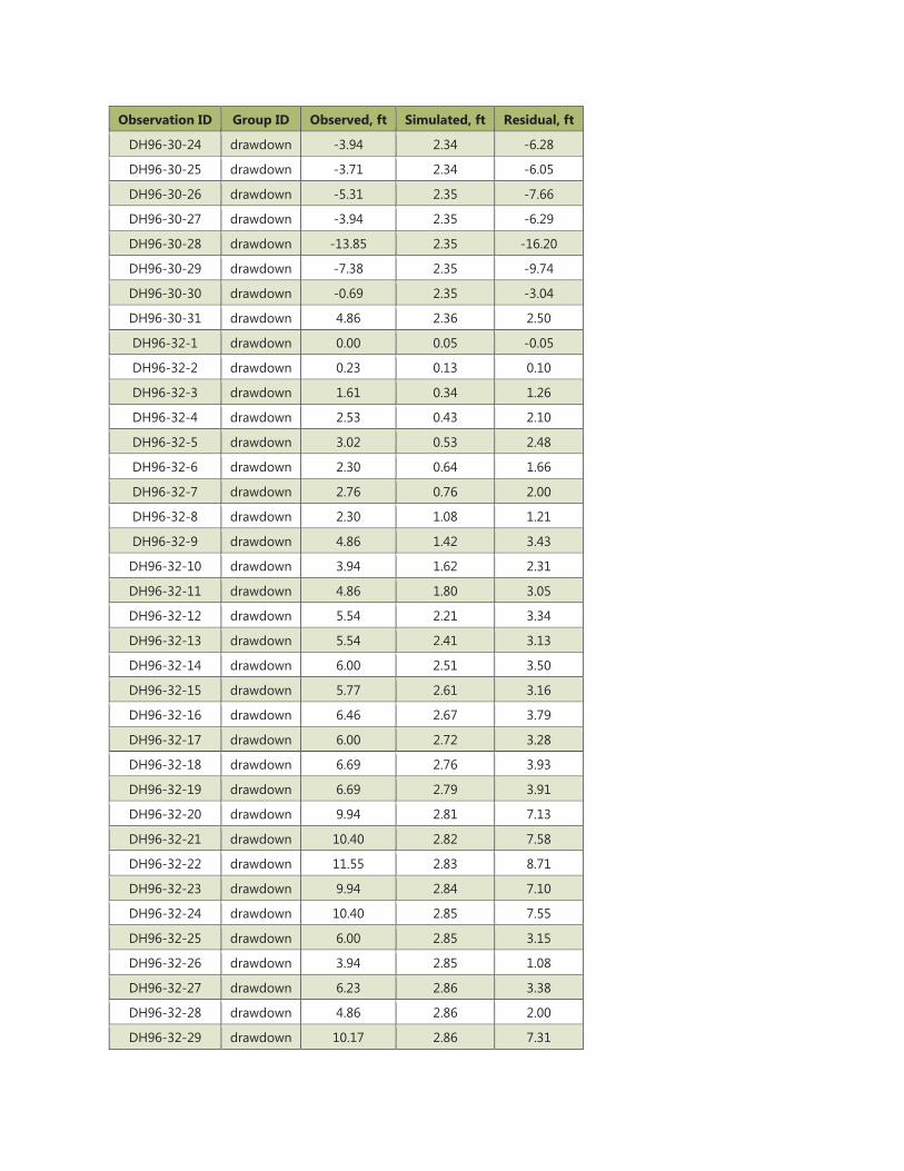
Observation ID Group ID Observed, ft Simulated, ft Residual, ft

DH96-30-24 drawdown -3.94 2.34 -6.28

DH96-30-25 drawdown -3.71 2.34 -6.05

DH96-30-26 drawdown -5.31 2.35 -7.66

DH96-30-27 drawdown -3.94 2.35 -6.29

DH96-30-28 drawdown -13.85 2.35 -16.20

DH96-30-29 drawdown -7.38 2.35 -9.74

DH96-30-30 drawdown -0.69 2.35 -3.04

DH96-30-31 drawdown 4.86 2.36 2.50

DH96-32-1 drawdown 0.00 0.05 -0.05

DH96-32-2 drawdown 0.23 0.13 0.10

DH96-32-3 drawdown 1.61 0.34 1.26

DH96-32-4 drawdown 2.53 0.43 2.10

DH96-32-5 drawdown 3.02 0.53 2.48

DH96-32-6 drawdown 2.30 0.64 1.66

DH96-32-7 drawdown 2.76 0.76 2.00

DH96-32-8 drawdown 2.30 1.08 1.21

DH96-32-9 drawdown 4.86 1.42 3.43

DH96-32-10 drawdown 3.94 1.62 2.31

DH96-32-11 drawdown 4.86 1.80 3.05

DH96-32-12 drawdown 5.54 2.21 3.34

DH96-32-13 drawdown 5.54 2.41 3.13

DH96-32-14 drawdown 6.00 2.51 3.50

DH96-32-15 drawdown 5.77 2.61 3.16

DH96-32-16 drawdown 6.46 2.67 3.79

DH96-32-17 drawdown 6.00 2.72 3.28

DH96-32-18 drawdown 6.69 2.76 3.93

DH96-32-19 drawdown 6.69 2.79 3.91

DH96-32-20 drawdown 9.94 2.81 7.13

DH96-32-21 drawdown 10.40 2.82 7.58

DH96-32-22 drawdown 11.55 2.83 8.71

DH96-32-23 drawdown 9.94 2.84 7.10

DH96-32-24 drawdown 10.40 2.85 7.55

DH96-32-25 drawdown 6.00 2.85 3.15

DH96-32-26 drawdown 3.94 2.85 1.08

DH96-32-27 drawdown 6.23 2.86 3.38

DH96-32-28 drawdown 4.86 2.86 2.00

DH96-32-29 drawdown 10.17 2.86 7.31

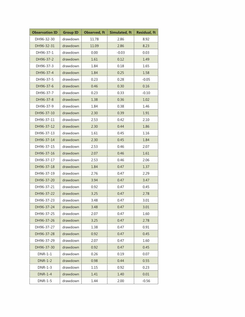
Observation ID Group ID Observed, ft Simulated, ft Residual, ft

DH96-32-30 drawdown 11.78 2.86 8.92

DH96-32-31 drawdown 11.09 2.86 8.23

DH96-37-1 drawdown 0.00 -0.03 0.03

DH96-37-2 drawdown 1.61 0.12 1.49

DH96-37-3 drawdown 1.84 0.18 1.65

DH96-37-4 drawdown 1.84 0.25 1.58

DH96-37-5 drawdown 0.23 0.28 -0.05

DH96-37-6 drawdown 0.46 0.30 0.16

DH96-37-7 drawdown 0.23 0.33 -0.10

DH96-37-8 drawdown 1.38 0.36 1.02

DH96-37-9 drawdown 1.84 0.38 1.46

DH96-37-10 drawdown 2.30 0.39 1.91

DH96-37-11 drawdown 2.53 0.42 2.10

DH96-37-12 drawdown 2.30 0.44 1.86

DH96-37-13 drawdown 1.61 0.45 1.16

DH96-37-14 drawdown 2.30 0.45 1.84

DH96-37-15 drawdown 2.53 0.46 2.07

DH96-37-16 drawdown 2.07 0.46 1.61

DH96-37-17 drawdown 2.53 0.46 2.06

DH96-37-18 drawdown 1.84 0.47 1.37

DH96-37-19 drawdown 2.76 0.47 2.29

DH96-37-20 drawdown 3.94 0.47 3.47

DH96-37-21 drawdown 0.92 0.47 0.45

DH96-37-22 drawdown 3.25 0.47 2.78

DH96-37-23 drawdown 3.48 0.47 3.01

DH96-37-24 drawdown 3.48 0.47 3.01

DH96-37-25 drawdown 2.07 0.47 1.60

DH96-37-26 drawdown 3.25 0.47 2.78

DH96-37-27 drawdown 1.38 0.47 0.91

DH96-37-28 drawdown 0.92 0.47 0.45

DH96-37-29 drawdown 2.07 0.47 1.60

DH96-37-30 drawdown 0.92 0.47 0.45

DNR-1-1 drawdown 0.26 0.19 0.07

DNR-1-2 drawdown 0.98 0.44 0.55

DNR-1-3 drawdown 1.15 0.92 0.23

DNR-1-4 drawdown 1.41 1.40 0.01

DNR-1-5 drawdown 1.44 2.00 -0.56

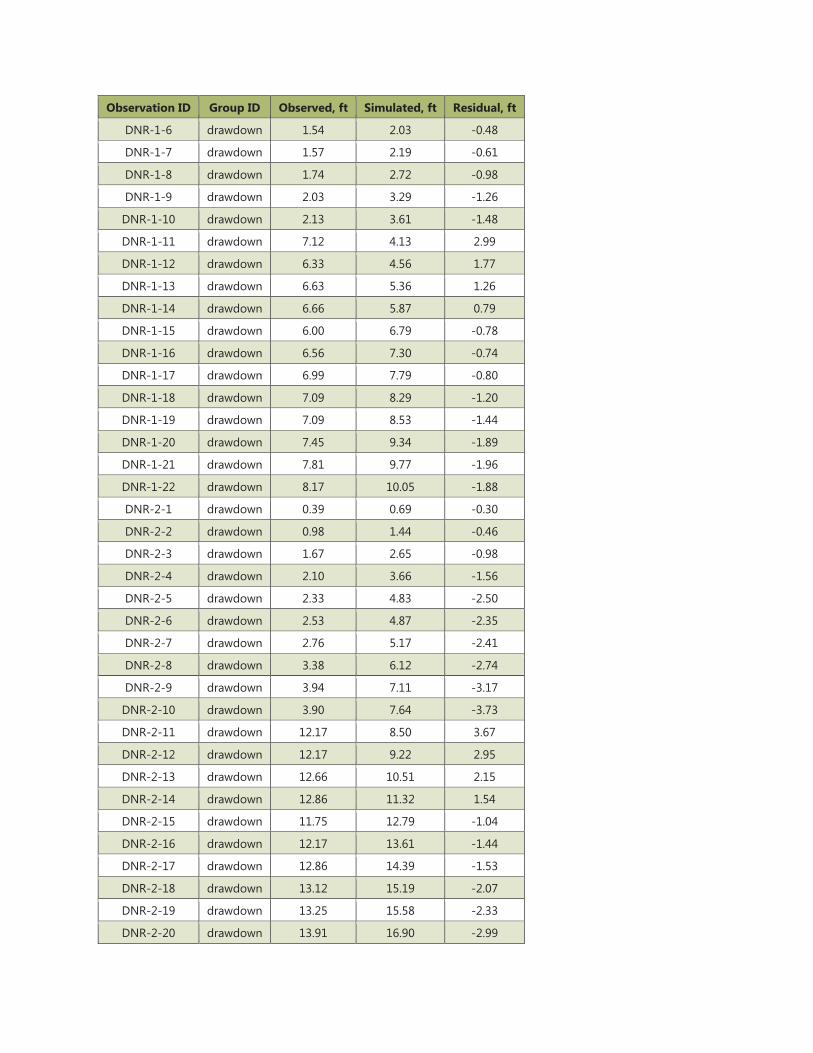
Observation ID Group ID Observed, ft Simulated, ft Residual, ft

DNR-1-6 drawdown 1.54 2.03 -0.48

DNR-1-7 drawdown 1.57 2.19 -0.61

DNR-1-8 drawdown 1.74 2.72 -0.98

DNR-1-9 drawdown 2.03 3.29 -1.26

DNR-1-10 drawdown 2.13 3.61 -1.48

DNR-1-11 drawdown 7.12 4.13 2.99

DNR-1-12 drawdown 6.33 4.56 1.77

DNR-1-13 drawdown 6.63 5.36 1.26

DNR-1-14 drawdown 6.66 5.87 0.79

DNR-1-15 drawdown 6.00 6.79 -0.78

DNR-1-16 drawdown 6.56 7.30 -0.74

DNR-1-17 drawdown 6.99 7.79 -0.80

DNR-1-18 drawdown 7.09 8.29 -1.20

DNR-1-19 drawdown 7.09 8.53 -1.44

DNR-1-20 drawdown 7.45 9.34 -1.89

DNR-1-21 drawdown 7.81 9.77 -1.96

DNR-1-22 drawdown 8.17 10.05 -1.88

DNR-2-1 drawdown 0.39 0.69 -0.30

DNR-2-2 drawdown 0.98 1.44 -0.46

DNR-2-3 drawdown 1.67 2.65 -0.98

DNR-2-4 drawdown 2.10 3.66 -1.56

DNR-2-5 drawdown 2.33 4.83 -2.50

DNR-2-6 drawdown 2.53 4.87 -2.35

DNR-2-7 drawdown 2.76 5.17 -2.41

DNR-2-8 drawdown 3.38 6.12 -2.74

DNR-2-9 drawdown 3.94 7.11 -3.17

DNR-2-10 drawdown 3.90 7.64 -3.73

DNR-2-11 drawdown 12.17 8.50 3.67

DNR-2-12 drawdown 12.17 9.22 2.95

DNR-2-13 drawdown 12.66 10.51 2.15

DNR-2-14 drawdown 12.86 11.32 1.54

DNR-2-15 drawdown 11.75 12.79 -1.04

DNR-2-16 drawdown 12.17 13.61 -1.44

DNR-2-17 drawdown 12.86 14.39 -1.53

DNR-2-18 drawdown 13.12 15.19 -2.07

DNR-2-19 drawdown 13.25 15.58 -2.33

DNR-2-20 drawdown 13.91 16.90 -2.99

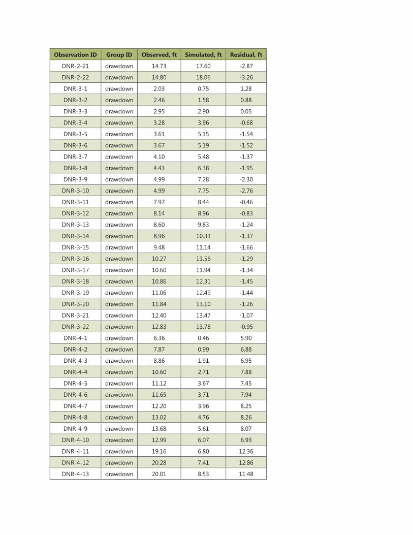
Observation ID Group ID Observed, ft Simulated, ft Residual, ft

DNR-2-21 drawdown 14.73 17.60 -2.87

DNR-2-22 drawdown 14.80 18.06 -3.26

DNR-3-1 drawdown 2.03 0.75 1.28

DNR-3-2 drawdown 2.46 1.58 0.88

DNR-3-3 drawdown 2.95 2.90 0.05

DNR-3-4 drawdown 3.28 3.96 -0.68

DNR-3-5 drawdown 3.61 5.15 -1.54

DNR-3-6 drawdown 3.67 5.19 -1.52

DNR-3-7 drawdown 4.10 5.48 -1.37

DNR-3-8 drawdown 4.43 6.38 -1.95

DNR-3-9 drawdown 4.99 7.28 -2.30

DNR-3-10 drawdown 4.99 7.75 -2.76

DNR-3-11 drawdown 7.97 8.44 -0.46

DNR-3-12 drawdown 8.14 8.96 -0.83

DNR-3-13 drawdown 8.60 9.83 -1.24

DNR-3-14 drawdown 8.96 10.33 -1.37

DNR-3-15 drawdown 9.48 11.14 -1.66

DNR-3-16 drawdown 10.27 11.56 -1.29

DNR-3-17 drawdown 10.60 11.94 -1.34

DNR-3-18 drawdown 10.86 12.31 -1.45

DNR-3-19 drawdown 11.06 12.49 -1.44

DNR-3-20 drawdown 11.84 13.10 -1.26

DNR-3-21 drawdown 12.40 13.47 -1.07

DNR-3-22 drawdown 12.83 13.78 -0.95

DNR-4-1 drawdown 6.36 0.46 5.90

DNR-4-2 drawdown 7.87 0.99 6.88

DNR-4-3 drawdown 8.86 1.91 6.95

DNR-4-4 drawdown 10.60 2.71 7.88

DNR-4-5 drawdown 11.12 3.67 7.45

DNR-4-6 drawdown 11.65 3.71 7.94

DNR-4-7 drawdown 12.20 3.96 8.25

DNR-4-8 drawdown 13.02 4.76 8.26

DNR-4-9 drawdown 13.68 5.61 8.07

DNR-4-10 drawdown 12.99 6.07 6.93

DNR-4-11 drawdown 19.16 6.80 12.36

DNR-4-12 drawdown 20.28 7.41 12.86

DNR-4-13 drawdown 20.01 8.53 11.48

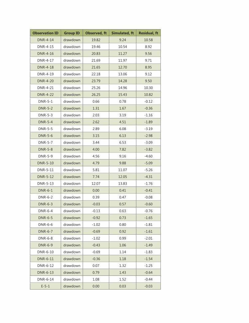
Observation ID Group ID Observed, ft Simulated, ft Residual, ft

DNR-4-14 drawdown 19.82 9.24 10.58

DNR-4-15 drawdown 19.46 10.54 8.92

DNR-4-16 drawdown 20.83 11.27 9.56

DNR-4-17 drawdown 21.69 11.97 9.71

DNR-4-18 drawdown 21.65 12.70 8.95

DNR-4-19 drawdown 22.18 13.06 9.12

DNR-4-20 drawdown 23.79 14.28 9.50

DNR-4-21 drawdown 25.26 14.96 10.30

DNR-4-22 drawdown 26.25 15.43 10.82

DNR-5-1 drawdown 0.66 0.78 -0.12

DNR-5-2 drawdown 1.31 1.67 -0.36

DNR-5-3 drawdown 2.03 3.19 -1.16

DNR-5-4 drawdown 2.62 4.51 -1.89

DNR-5-5 drawdown 2.89 6.08 -3.19

DNR-5-6 drawdown 3.15 6.13 -2.98

DNR-5-7 drawdown 3.44 6.53 -3.09

DNR-5-8 drawdown 4.00 7.82 -3.82

DNR-5-9 drawdown 4.56 9.16 -4.60

DNR-5-10 drawdown 4.79 9.88 -5.09

DNR-5-11 drawdown 5.81 11.07 -5.26

DNR-5-12 drawdown 7.74 12.05 -4.31

DNR-5-13 drawdown 12.07 13.83 -1.76

DNR-6-1 drawdown 0.00 0.41 -0.41

DNR-6-2 drawdown 0.39 0.47 -0.08

DNR-6-3 drawdown -0.03 0.57 -0.60

DNR-6-4 drawdown -0.13 0.63 -0.76

DNR-6-5 drawdown -0.92 0.73 -1.65

DNR-6-6 drawdown -1.02 0.80 -1.81

DNR-6-7 drawdown -0.69 0.92 -1.61

DNR-6-8 drawdown -1.02 0.99 -2.01

DNR-6-9 drawdown -0.43 1.06 -1.49

DNR-6-10 drawdown -0.69 1.14 -1.83

DNR-6-11 drawdown -0.36 1.18 -1.54

DNR-6-12 drawdown 0.07 1.32 -1.25

DNR-6-13 drawdown 0.79 1.43 -0.64

DNR-6-14 drawdown 1.08 1.52 -0.44

E-5-1 drawdown 0.00 0.03 -0.03

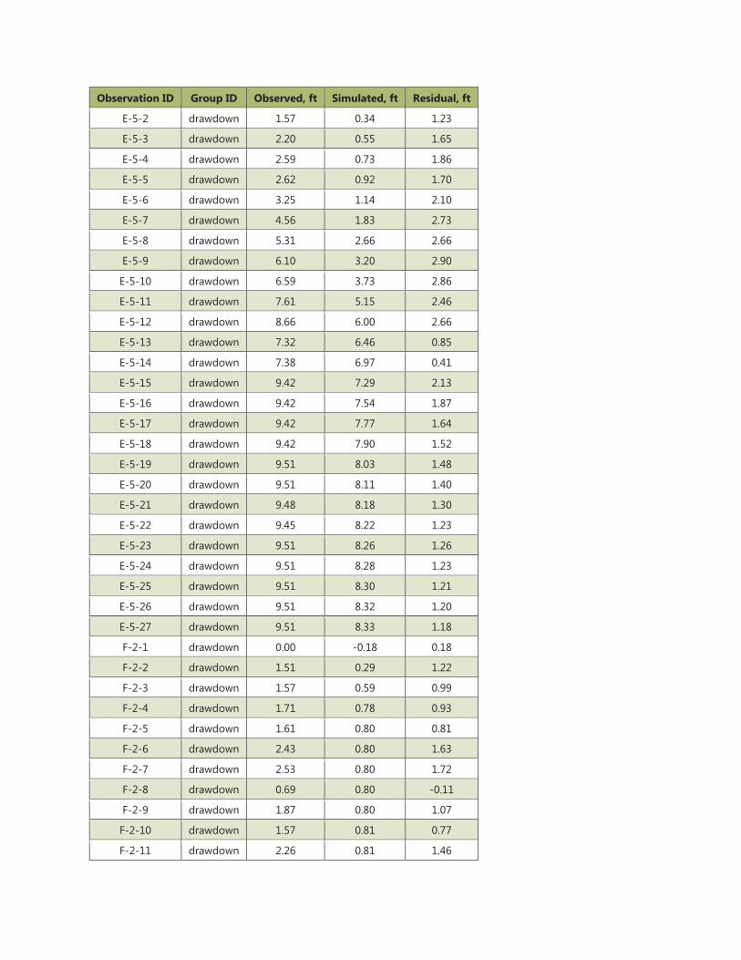
Observation ID Group ID Observed, ft Simulated, ft Residual, ft

E-5-2 drawdown 1.57 0.34 1.23

E-5-3 drawdown 2.20 0.55 1.65

E-5-4 drawdown 2.59 0.73 1.86

E-5-5 drawdown 2.62 0.92 1.70

E-5-6 drawdown 3.25 1.14 2.10

E-5-7 drawdown 4.56 1.83 2.73

E-5-8 drawdown 5.31 2.66 2.66

E-5-9 drawdown 6.10 3.20 2.90

E-5-10 drawdown 6.59 3.73 2.86

E-5-11 drawdown 7.61 5.15 2.46

E-5-12 drawdown 8.66 6.00 2.66

E-5-13 drawdown 7.32 6.46 0.85

E-5-14 drawdown 7.38 6.97 0.41

E-5-15 drawdown 9.42 7.29 2.13

E-5-16 drawdown 9.42 7.54 1.87

E-5-17 drawdown 9.42 7.77 1.64

E-5-18 drawdown 9.42 7.90 1.52

E-5-19 drawdown 9.51 8.03 1.48

E-5-20 drawdown 9.51 8.11 1.40

E-5-21 drawdown 9.48 8.18 1.30

E-5-22 drawdown 9.45 8.22 1.23

E-5-23 drawdown 9.51 8.26 1.26

E-5-24 drawdown 9.51 8.28 1.23

E-5-25 drawdown 9.51 8.30 1.21

E-5-26 drawdown 9.51 8.32 1.20

E-5-27 drawdown 9.51 8.33 1.18

F-2-1 drawdown 0.00 -0.18 0.18

F-2-2 drawdown 1.51 0.29 1.22

F-2-3 drawdown 1.57 0.59 0.99

F-2-4 drawdown 1.71 0.78 0.93

F-2-5 drawdown 1.61 0.80 0.81

F-2-6 drawdown 2.43 0.80 1.63

F-2-7 drawdown 2.53 0.80 1.72

F-2-8 drawdown 0.69 0.80 -0.11

F-2-9 drawdown 1.87 0.80 1.07

F-2-10 drawdown 1.57 0.81 0.77

F-2-11 drawdown 2.26 0.81 1.46

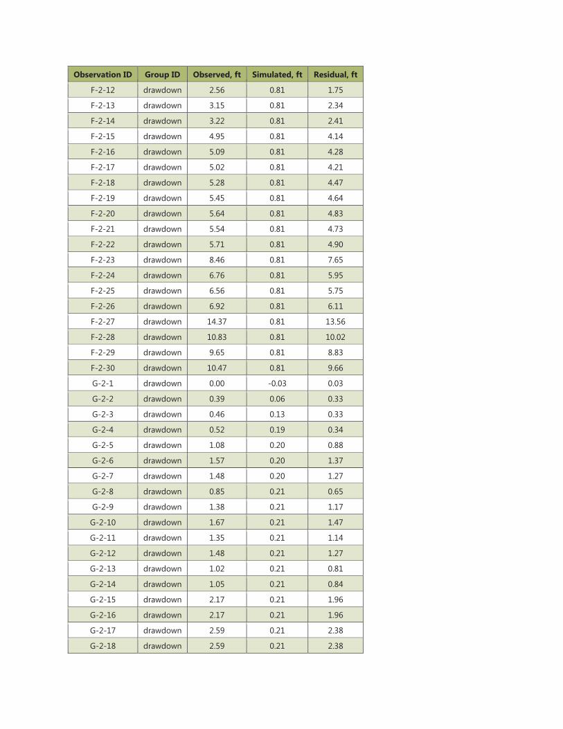
Observation ID Group ID Observed, ft Simulated, ft Residual, ft

F-2-12 drawdown 2.56 0.81 1.75

F-2-13 drawdown 3.15 0.81 2.34

F-2-14 drawdown 3.22 0.81 2.41

F-2-15 drawdown 4.95 0.81 4.14

F-2-16 drawdown 5.09 0.81 4.28

F-2-17 drawdown 5.02 0.81 4.21

F-2-18 drawdown 5.28 0.81 4.47

F-2-19 drawdown 5.45 0.81 4.64

F-2-20 drawdown 5.64 0.81 4.83

F-2-21 drawdown 5.54 0.81 4.73

F-2-22 drawdown 5.71 0.81 4.90

F-2-23 drawdown 8.46 0.81 7.65

F-2-24 drawdown 6.76 0.81 5.95

F-2-25 drawdown 6.56 0.81 5.75

F-2-26 drawdown 6.92 0.81 6.11

F-2-27 drawdown 14.37 0.81 13.56

F-2-28 drawdown 10.83 0.81 10.02

F-2-29 drawdown 9.65 0.81 8.83

F-2-30 drawdown 10.47 0.81 9.66

G-2-1 drawdown 0.00 -0.03 0.03

G-2-2 drawdown 0.39 0.06 0.33

G-2-3 drawdown 0.46 0.13 0.33

G-2-4 drawdown 0.52 0.19 0.34

G-2-5 drawdown 1.08 0.20 0.88

G-2-6 drawdown 1.57 0.20 1.37

G-2-7 drawdown 1.48 0.20 1.27

G-2-8 drawdown 0.85 0.21 0.65

G-2-9 drawdown 1.38 0.21 1.17

G-2-10 drawdown 1.67 0.21 1.47

G-2-11 drawdown 1.35 0.21 1.14

G-2-12 drawdown 1.48 0.21 1.27

G-2-13 drawdown 1.02 0.21 0.81

G-2-14 drawdown 1.05 0.21 0.84

G-2-15 drawdown 2.17 0.21 1.96

G-2-16 drawdown 2.17 0.21 1.96

G-2-17 drawdown 2.59 0.21 2.38

G-2-18 drawdown 2.59 0.21 2.38

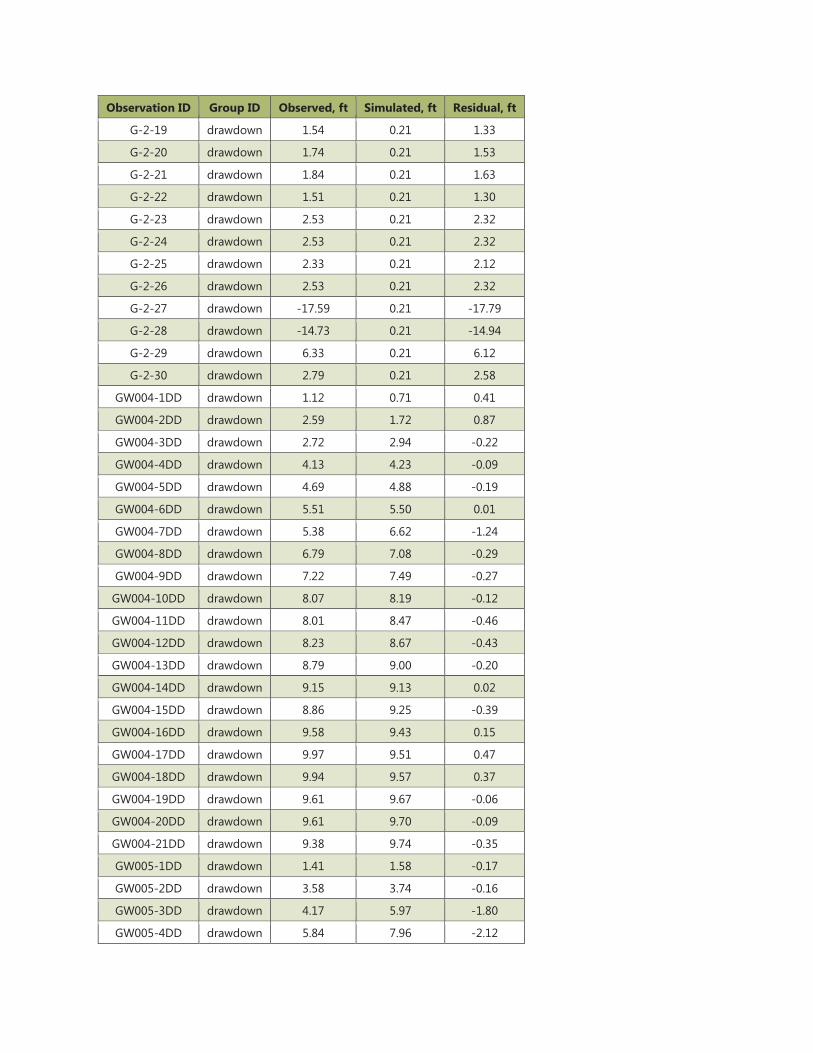
Observation ID Group ID Observed, ft Simulated, ft Residual, ft

G-2-19 drawdown 1.54 0.21 1.33

G-2-20 drawdown 1.74 0.21 1.53

G-2-21 drawdown 1.84 0.21 1.63

G-2-22 drawdown 1.51 0.21 1.30

G-2-23 drawdown 2.53 0.21 2.32

G-2-24 drawdown 2.53 0.21 2.32

G-2-25 drawdown 2.33 0.21 2.12

G-2-26 drawdown 2.53 0.21 2.32

G-2-27 drawdown -17.59 0.21 -17.79

G-2-28 drawdown -14.73 0.21 -14.94

G-2-29 drawdown 6.33 0.21 6.12

G-2-30 drawdown 2.79 0.21 2.58

GW004-1DD drawdown 1.12 0.71 0.41

GW004-2DD drawdown 2.59 1.72 0.87

GW004-3DD drawdown 2.72 2.94 -0.22

GW004-4DD drawdown 4.13 4.23 -0.09

GW004-5DD drawdown 4.69 4.88 -0.19

GW004-6DD drawdown 5.51 5.50 0.01

GW004-7DD drawdown 5.38 6.62 -1.24

GW004-8DD drawdown 6.79 7.08 -0.29

GW004-9DD drawdown 7.22 7.49 -0.27

GW004-10DD drawdown 8.07 8.19 -0.12

GW004-11DD drawdown 8.01 8.47 -0.46

GW004-12DD drawdown 8.23 8.67 -0.43

GW004-13DD drawdown 8.79 9.00 -0.20

GW004-14DD drawdown 9.15 9.13 0.02

GW004-15DD drawdown 8.86 9.25 -0.39

GW004-16DD drawdown 9.58 9.43 0.15

GW004-17DD drawdown 9.97 9.51 0.47

GW004-18DD drawdown 9.94 9.57 0.37

GW004-19DD drawdown 9.61 9.67 -0.06

GW004-20DD drawdown 9.61 9.70 -0.09

GW004-21DD drawdown 9.38 9.74 -0.35

GW005-1DD drawdown 1.41 1.58 -0.17

GW005-2DD drawdown 3.58 3.74 -0.16

GW005-3DD drawdown 4.17 5.97 -1.80

GW005-4DD drawdown 5.84 7.96 -2.12

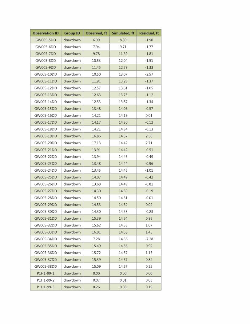
Observation ID Group ID Observed, ft Simulated, ft Residual, ft

GW005-5DD drawdown 6.99 8.89 -1.90

GW005-6DD drawdown 7.94 9.71 -1.77

GW005-7DD drawdown 9.78 11.59 -1.81

GW005-8DD drawdown 10.53 12.04 -1.51

GW005-9DD drawdown 11.45 12.78 -1.33

GW005-10DD drawdown 10.50 13.07 -2.57

GW005-11DD drawdown 11.91 13.28 -1.37

GW005-12DD drawdown 12.57 13.61 -1.05

GW005-13DD drawdown 12.63 13.75 -1.12

GW005-14DD drawdown 12.53 13.87 -1.34

GW005-15DD drawdown 13.48 14.06 -0.57

GW005-16DD drawdown 14.21 14.19 0.01

GW005-17DD drawdown 14.17 14.30 -0.12

GW005-18DD drawdown 14.21 14.34 -0.13

GW005-19DD drawdown 16.86 14.37 2.50

GW005-20DD drawdown 17.13 14.42 2.71

GW005-21DD drawdown 13.91 14.42 -0.51

GW005-22DD drawdown 13.94 14.43 -0.49

GW005-23DD drawdown 13.48 14.44 -0.96

GW005-24DD drawdown 13.45 14.46 -1.01

GW005-25DD drawdown 14.07 14.49 -0.42

GW005-26DD drawdown 13.68 14.49 -0.81

GW005-27DD drawdown 14.30 14.50 -0.19

GW005-28DD drawdown 14.50 14.51 -0.01

GW005-29DD drawdown 14.53 14.52 0.02

GW005-30DD drawdown 14.30 14.53 -0.23

GW005-31DD drawdown 15.39 14.54 0.85

GW005-32DD drawdown 15.62 14.55 1.07

GW005-33DD drawdown 16.01 14.56 1.45

GW005-34DD drawdown 7.28 14.56 -7.28

GW005-35DD drawdown 15.49 14.56 0.92

GW005-36DD drawdown 15.72 14.57 1.15

GW005-37DD drawdown 15.39 14.57 0.82

GW005-38DD drawdown 15.09 14.57 0.52

P1H1-99-1 drawdown 0.00 0.00 0.00

P1H1-99-2 drawdown 0.07 0.01 0.05

P1H1-99-3 drawdown 0.26 0.08 0.19

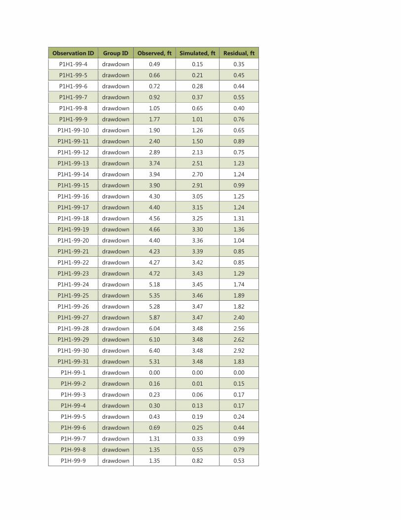
Observation ID Group ID Observed, ft Simulated, ft Residual, ft

P1H1-99-4 drawdown 0.49 0.15 0.35

P1H1-99-5 drawdown 0.66 0.21 0.45

P1H1-99-6 drawdown 0.72 0.28 0.44

P1H1-99-7 drawdown 0.92 0.37 0.55

P1H1-99-8 drawdown 1.05 0.65 0.40

P1H1-99-9 drawdown 1.77 1.01 0.76

P1H1-99-10 drawdown 1.90 1.26 0.65

P1H1-99-11 drawdown 2.40 1.50 0.89

P1H1-99-12 drawdown 2.89 2.13 0.75

P1H1-99-13 drawdown 3.74 2.51 1.23

P1H1-99-14 drawdown 3.94 2.70 1.24

P1H1-99-15 drawdown 3.90 2.91 0.99

P1H1-99-16 drawdown 4.30 3.05 1.25

P1H1-99-17 drawdown 4.40 3.15 1.24

P1H1-99-18 drawdown 4.56 3.25 1.31

P1H1-99-19 drawdown 4.66 3.30 1.36

P1H1-99-20 drawdown 4.40 3.36 1.04

P1H1-99-21 drawdown 4.23 3.39 0.85

P1H1-99-22 drawdown 4.27 3.42 0.85

P1H1-99-23 drawdown 4.72 3.43 1.29

P1H1-99-24 drawdown 5.18 3.45 1.74

P1H1-99-25 drawdown 5.35 3.46 1.89

P1H1-99-26 drawdown 5.28 3.47 1.82

P1H1-99-27 drawdown 5.87 3.47 2.40

P1H1-99-28 drawdown 6.04 3.48 2.56

P1H1-99-29 drawdown 6.10 3.48 2.62

P1H1-99-30 drawdown 6.40 3.48 2.92

P1H1-99-31 drawdown 5.31 3.48 1.83

P1H-99-1 drawdown 0.00 0.00 0.00

P1H-99-2 drawdown 0.16 0.01 0.15

P1H-99-3 drawdown 0.23 0.06 0.17

P1H-99-4 drawdown 0.30 0.13 0.17

P1H-99-5 drawdown 0.43 0.19 0.24

P1H-99-6 drawdown 0.69 0.25 0.44

P1H-99-7 drawdown 1.31 0.33 0.99

P1H-99-8 drawdown 1.35 0.55 0.79

P1H-99-9 drawdown 1.35 0.82 0.53

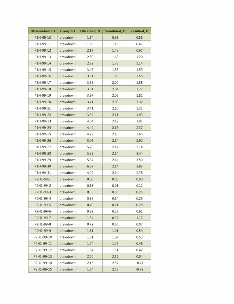
Observation ID Group ID Observed, ft Simulated, ft Residual, ft

P1H-99-10 drawdown 1.54 0.98 0.56

P1H-99-11 drawdown 1.80 1.13 0.67

P1H-99-12 drawdown 2.17 1.49 0.67

P1H-99-13 drawdown 2.89 1.69 1.20

P1H-99-14 drawdown 2.92 1.78 1.14

P1H-99-15 drawdown 3.48 1.88 1.59

P1H-99-16 drawdown 3.51 1.95 1.56

P1H-99-17 drawdown 3.58 2.00 1.58

P1H-99-18 drawdown 3.81 2.04 1.77

P1H-99-19 drawdown 3.87 2.06 1.81

P1H-99-20 drawdown 3.41 2.09 1.32

P1H-99-21 drawdown 3.41 2.10 1.31

P1H-99-22 drawdown 3.54 2.11 1.43

P1H-99-23 drawdown 4.04 2.12 1.91

P1H-99-24 drawdown 4.49 2.13 2.37

P1H-99-25 drawdown 4.79 2.13 2.66

P1H-99-26 drawdown 5.05 2.14 2.92

P1H-99-27 drawdown 5.28 2.14 3.14

P1H-99-28 drawdown 5.58 2.14 3.44

P1H-99-29 drawdown 5.64 2.14 3.50

P1H-99-30 drawdown 6.07 2.14 3.93

P1H-99-31 drawdown 4.92 2.14 2.78

P2H1-99-1 drawdown 0.00 0.00 0.00

P2H1-99-2 drawdown 0.13 0.01 0.12

P2H1-99-3 drawdown 0.33 0.08 0.25

P2H1-99-4 drawdown 0.39 0.14 0.25

P2H1-99-5 drawdown 0.49 0.21 0.28

P2H1-99-6 drawdown 0.89 0.28 0.61

P2H1-99-7 drawdown 1.54 0.37 1.17

P2H1-99-8 drawdown 0.72 0.65 0.07

P2H1-99-9 drawdown 1.61 1.01 0.59

P2H1-99-10 drawdown 1.61 1.07 0.53

P2H1-99-11 drawdown 1.74 1.26 0.48

P2H1-99-12 drawdown 1.94 1.51 0.42

P2H1-99-13 drawdown 2.20 2.15 0.04

P2H1-99-14 drawdown 2.13 2.54 -0.41

P2H1-99-15 drawdown 1.84 2.73 -0.89

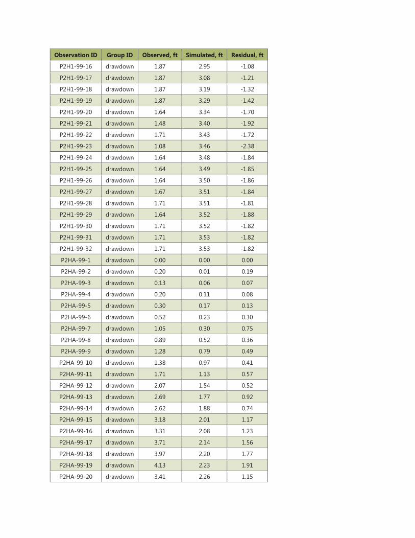
Observation ID Group ID Observed, ft Simulated, ft Residual, ft

P2H1-99-16 drawdown 1.87 2.95 -1.08

P2H1-99-17 drawdown 1.87 3.08 -1.21

P2H1-99-18 drawdown 1.87 3.19 -1.32

P2H1-99-19 drawdown 1.87 3.29 -1.42

P2H1-99-20 drawdown 1.64 3.34 -1.70

P2H1-99-21 drawdown 1.48 3.40 -1.92

P2H1-99-22 drawdown 1.71 3.43 -1.72

P2H1-99-23 drawdown 1.08 3.46 -2.38

P2H1-99-24 drawdown 1.64 3.48 -1.84

P2H1-99-25 drawdown 1.64 3.49 -1.85

P2H1-99-26 drawdown 1.64 3.50 -1.86

P2H1-99-27 drawdown 1.67 3.51 -1.84

P2H1-99-28 drawdown 1.71 3.51 -1.81

P2H1-99-29 drawdown 1.64 3.52 -1.88

P2H1-99-30 drawdown 1.71 3.52 -1.82

P2H1-99-31 drawdown 1.71 3.53 -1.82

P2H1-99-32 drawdown 1.71 3.53 -1.82

P2HA-99-1 drawdown 0.00 0.00 0.00

P2HA-99-2 drawdown 0.20 0.01 0.19

P2HA-99-3 drawdown 0.13 0.06 0.07

P2HA-99-4 drawdown 0.20 0.11 0.08

P2HA-99-5 drawdown 0.30 0.17 0.13

P2HA-99-6 drawdown 0.52 0.23 0.30

P2HA-99-7 drawdown 1.05 0.30 0.75

P2HA-99-8 drawdown 0.89 0.52 0.36

P2HA-99-9 drawdown 1.28 0.79 0.49

P2HA-99-10 drawdown 1.38 0.97 0.41

P2HA-99-11 drawdown 1.71 1.13 0.57

P2HA-99-12 drawdown 2.07 1.54 0.52

P2HA-99-13 drawdown 2.69 1.77 0.92

P2HA-99-14 drawdown 2.62 1.88 0.74

P2HA-99-15 drawdown 3.18 2.01 1.17

P2HA-99-16 drawdown 3.31 2.08 1.23

P2HA-99-17 drawdown 3.71 2.14 1.56

P2HA-99-18 drawdown 3.97 2.20 1.77

P2HA-99-19 drawdown 4.13 2.23 1.91

P2HA-99-20 drawdown 3.41 2.26 1.15

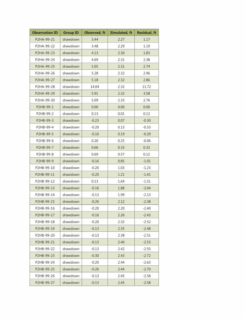
Observation ID Group ID Observed, ft Simulated, ft Residual, ft

P2HA-99-21 drawdown 3.44 2.27 1.17

P2HA-99-22 drawdown 3.48 2.29 1.19

P2HA-99-23 drawdown 4.13 2.30 1.83

P2HA-99-24 drawdown 4.69 2.31 2.38

P2HA-99-25 drawdown 5.05 2.31 2.74

P2HA-99-26 drawdown 5.28 2.32 2.96

P2HA-99-27 drawdown 5.18 2.32 2.86

P2HA-99-28 drawdown 14.04 2.32 11.72

P2HA-99-29 drawdown 5.91 2.32 3.58

P2HA-99-30 drawdown 5.09 2.33 2.76

P2HB-99-1 drawdown 0.00 0.00 0.00

P2HB-99-2 drawdown 0.13 0.01 0.12

P2HB-99-3 drawdown -0.23 0.07 -0.30

P2HB-99-4 drawdown -0.20 0.13 -0.33

P2HB-99-5 drawdown -0.10 0.19 -0.29

P2HB-99-6 drawdown 0.20 0.25 -0.06

P2HB-99-7 drawdown 0.66 0.33 0.33

P2HB-99-8 drawdown 0.69 0.57 0.12

P2HB-99-9 drawdown -0.16 0.85 -1.01

P2HB-99-10 drawdown -0.20 1.03 -1.23

P2HB-99-11 drawdown -0.20 1.21 -1.41

P2HB-99-12 drawdown 0.13 1.64 -1.51

P2HB-99-13 drawdown -0.16 1.88 -2.04

P2HB-99-14 drawdown -0.13 1.99 -2.13

P2HB-99-15 drawdown -0.26 2.12 -2.38

P2HB-99-16 drawdown -0.20 2.20 -2.40

P2HB-99-17 drawdown -0.16 2.26 -2.43

P2HB-99-18 drawdown -0.20 2.32 -2.52

P2HB-99-19 drawdown -0.13 2.35 -2.48

P2HB-99-20 drawdown -0.13 2.38 -2.51

P2HB-99-21 drawdown -0.13 2.40 -2.53

P2HB-99-22 drawdown -0.13 2.42 -2.55

P2HB-99-23 drawdown -0.30 2.43 -2.72

P2HB-99-24 drawdown -0.20 2.44 -2.63

P2HB-99-25 drawdown -0.26 2.44 -2.70

P2HB-99-26 drawdown -0.13 2.45 -2.58

P2HB-99-27 drawdown -0.13 2.45 -2.58

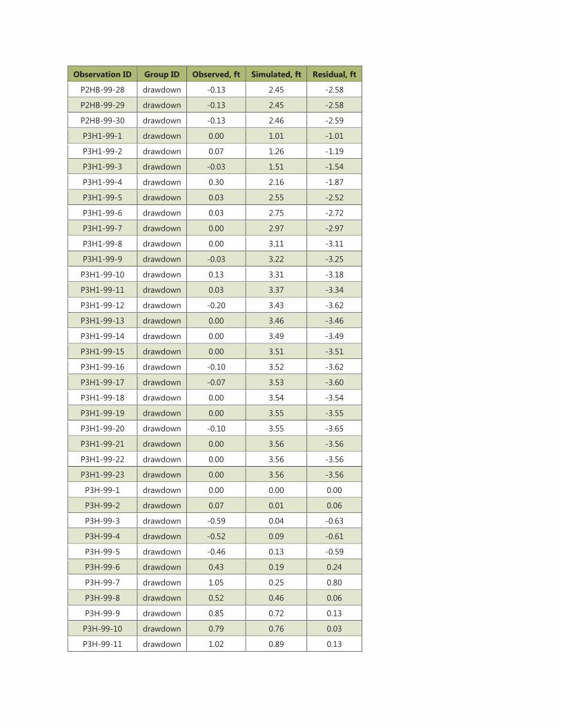
Observation ID Group ID Observed, ft Simulated, ft Residual, ft

P2HB-99-28 drawdown -0.13 2.45 -2.58

P2HB-99-29 drawdown -0.13 2.45 -2.58

P2HB-99-30 drawdown -0.13 2.46 -2.59

P3H1-99-1 drawdown 0.00 1.01 -1.01

P3H1-99-2 drawdown 0.07 1.26 -1.19

P3H1-99-3 drawdown -0.03 1.51 -1.54

P3H1-99-4 drawdown 0.30 2.16 -1.87

P3H1-99-5 drawdown 0.03 2.55 -2.52

P3H1-99-6 drawdown 0.03 2.75 -2.72

P3H1-99-7 drawdown 0.00 2.97 -2.97

P3H1-99-8 drawdown 0.00 3.11 -3.11

P3H1-99-9 drawdown -0.03 3.22 -3.25

P3H1-99-10 drawdown 0.13 3.31 -3.18

P3H1-99-11 drawdown 0.03 3.37 -3.34

P3H1-99-12 drawdown -0.20 3.43 -3.62

P3H1-99-13 drawdown 0.00 3.46 -3.46

P3H1-99-14 drawdown 0.00 3.49 -3.49

P3H1-99-15 drawdown 0.00 3.51 -3.51

P3H1-99-16 drawdown -0.10 3.52 -3.62

P3H1-99-17 drawdown -0.07 3.53 -3.60

P3H1-99-18 drawdown 0.00 3.54 -3.54

P3H1-99-19 drawdown 0.00 3.55 -3.55

P3H1-99-20 drawdown -0.10 3.55 -3.65

P3H1-99-21 drawdown 0.00 3.56 -3.56

P3H1-99-22 drawdown 0.00 3.56 -3.56

P3H1-99-23 drawdown 0.00 3.56 -3.56

P3H-99-1 drawdown 0.00 0.00 0.00

P3H-99-2 drawdown 0.07 0.01 0.06

P3H-99-3 drawdown -0.59 0.04 -0.63

P3H-99-4 drawdown -0.52 0.09 -0.61

P3H-99-5 drawdown -0.46 0.13 -0.59

P3H-99-6 drawdown 0.43 0.19 0.24

P3H-99-7 drawdown 1.05 0.25 0.80

P3H-99-8 drawdown 0.52 0.46 0.06

P3H-99-9 drawdown 0.85 0.72 0.13

P3H-99-10 drawdown 0.79 0.76 0.03

P3H-99-11 drawdown 1.02 0.89 0.13

Observation ID Group ID Observed, ft Simulated, ft Residual, ft

P3H-99-12 drawdown 1.12 1.05 0.06

P3H-99-13 drawdown 1.18 1.46 -0.28

P3H-99-14 drawdown 1.35 1.70 -0.35

P3H-99-15 drawdown 1.67 1.81 -0.14

P3H-99-16 drawdown 2.13 1.93 0.20

P3H-99-17 drawdown 2.26 2.01 0.25

P3H-99-18 drawdown 3.31 2.07 1.24

P3H-99-19 drawdown 2.62 2.13 0.50

P3H-99-20 drawdown 3.22 2.16 1.06

P3H-99-21 drawdown 2.07 2.19 -0.12

P3H-99-22 drawdown 2.82 2.21 0.61

P3H-99-23 drawdown 2.92 2.23 0.69

P3H-99-24 drawdown 2.92 2.23 0.69

P3H-99-25 drawdown 3.67 2.24 1.43

P3H-99-26 drawdown 3.44 2.25 1.20

P3H-99-27 drawdown 3.35 2.25 1.09

P3H-99-28 drawdown 3.67 2.26 1.42

P3H-99-29 drawdown 3.67 2.26 1.42

P3H-99-30 drawdown 3.67 2.26 1.41

P3H-99-31 drawdown 3.67 2.26 1.41

P3H-99-32 drawdown 3.67 2.26 1.41

PN1J-99-1 drawdown 0.00 -0.05 0.05

PN1J-99-2 drawdown 0.23 -0.03 0.26

PN1J-99-3 drawdown 0.23 0.14 0.09

PN1J-99-4 drawdown 0.46 0.19 0.27

PN1J-99-5 drawdown 0.92 0.28 0.63

PN1J-99-6 drawdown 1.61 0.39 1.22

PN1J-99-7 drawdown 1.61 0.43 1.18

PN1J-99-8 drawdown 1.84 0.45 1.39

PN1J-99-9 drawdown 1.61 0.49 1.12

PN1J-99-10 drawdown 3.25 0.53 2.72

PN1J-99-11 drawdown 3.25 0.53 2.72

PN1J-99-12 drawdown 3.25 0.61 2.64

PN1J-99-13 drawdown 3.25 0.63 2.62

PN1J-99-14 drawdown 3.25 0.64 2.61

PN1J-99-15 drawdown 3.25 0.64 2.60

PN1J-99-16 drawdown 3.48 0.65 2.83

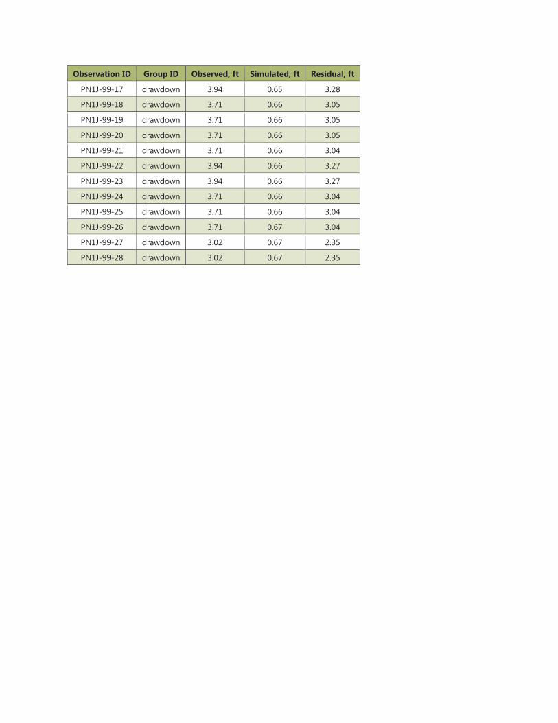
Observation ID Group ID Observed, ft Simulated, ft Residual, ft

PN1J-99-17 drawdown 3.94 0.65 3.28

PN1J-99-18 drawdown 3.71 0.66 3.05

PN1J-99-19 drawdown 3.71 0.66 3.05

PN1J-99-20 drawdown 3.71 0.66 3.05

PN1J-99-21 drawdown 3.71 0.66 3.04

PN1J-99-22 drawdown 3.94 0.66 3.27

PN1J-99-23 drawdown 3.94 0.66 3.27

PN1J-99-24 drawdown 3.71 0.66 3.04

PN1J-99-25 drawdown 3.71 0.66 3.04

PN1J-99-26 drawdown 3.71 0.67 3.04

PN1J-99-27 drawdown 3.02 0.67 2.35

PN1J-99-28 drawdown 3.02 0.67 2.35

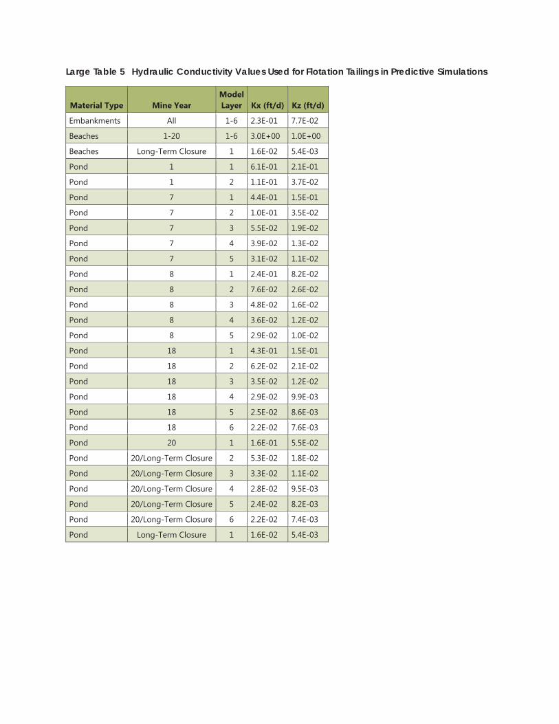
Large Table 5 Hydraulic Conductivity Values Used for Flotation Tailings in Predictive Simulations

Material Type Mine Year Model Layer Kx (ft/d) Kz (ft/d)

Embankments All 1-6 2.3E-01 7.7E-02

Beaches 1-20 1-6 3.0E+00 1.0E+00

Beaches Long-Term Closure 1 1.6E-02 5.4E-03

Pond 1 1 6.1E-01 2.1E-01

Pond 1 2 1.1E-01 3.7E-02

Pond 7 1 4.4E-01 1.5E-01

Pond 7 2 1.0E-01 3.5E-02

Pond 7 3 5.5E-02 1.9E-02

Pond 7 4 3.9E-02 1.3E-02

Pond 7 5 3.1E-02 1.1E-02

Pond 8 1 2.4E-01 8.2E-02

Pond 8 2 7.6E-02 2.6E-02

Pond 8 3 4.8E-02 1.6E-02

Pond 8 4 3.6E-02 1.2E-02

Pond 8 5 2.9E-02 1.0E-02

Pond 18 1 4.3E-01 1.5E-01

Pond 18 2 6.2E-02 2.1E-02

Pond 18 3 3.5E-02 1.2E-02

Pond 18 4 2.9E-02 9.9E-03

Pond 18 5 2.5E-02 8.6E-03

Pond 18 6 2.2E-02 7.6E-03

Pond 20 1 1.6E-01 5.5E-02

Pond 20/Long-Term Closure 2 5.3E-02 1.8E-02

Pond 20/Long-Term Closure 3 3.3E-02 1.1E-02

Pond 20/Long-Term Closure 4 2.8E-02 9.5E-03

Pond 20/Long-Term Closure 5 2.4E-02 8.2E-03

Pond 20/Long-Term Closure 6 2.2E-02 7.4E-03

Pond Long-Term Closure 1 1.6E-02 5.4E-03

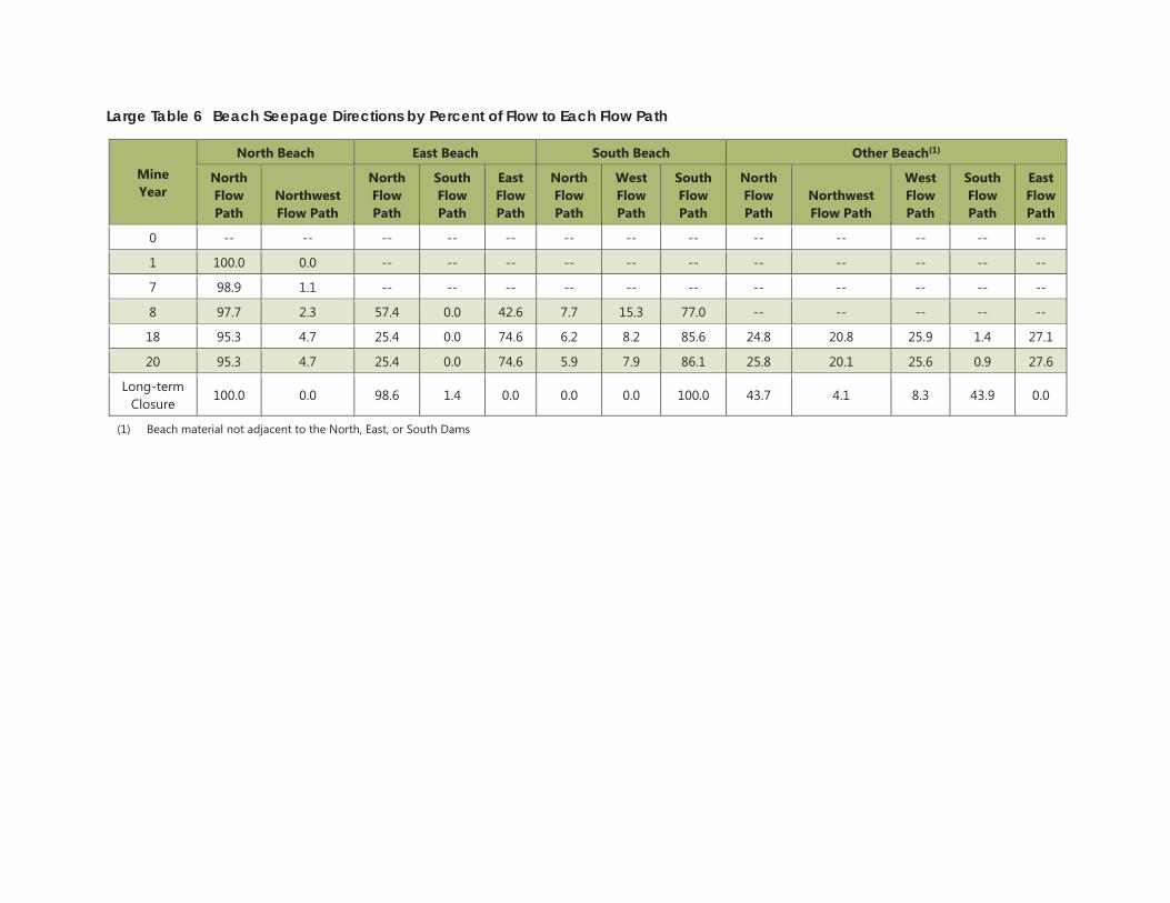
Large Table 6 Beach Seepage Directions by Percent of Flow to Each Flow Path

Mine Year

North Beach East Beach South Beach Other Beach(1)

North Flow Path

Northwest Flow Path

North Flow Path

South Flow Path

East Flow Path

North Flow Path

West Flow Path

South Flow Path

North Flow Path

Northwest Flow Path

West Flow Path

South Flow Path

East Flow Path

0 -- -- -- -- -- -- -- -- -- -- -- -- --

1 100.0 0.0 -- -- -- -- -- -- -- -- -- -- --

7 98.9 1.1 -- -- -- -- -- -- -- -- -- -- --

8 97.7 2.3 57.4 0.0 42.6 7.7 15.3 77.0 -- -- -- -- --

18 95.3 4.7 25.4 0.0 74.6 6.2 8.2 85.6 24.8 20.8 25.9 1.4 27.1

20 95.3 4.7 25.4 0.0 74.6 5.9 7.9 86.1 25.8 20.1 25.6 0.9 27.6

Long-term Closure

100.0 0.0 98.6 1.4 0.0 0.0 0.0 100.0 43.7 4.1 8.3 43.9 0.0

(1) Beach material not adjacent to the North, East, or South Dams

Large Figures

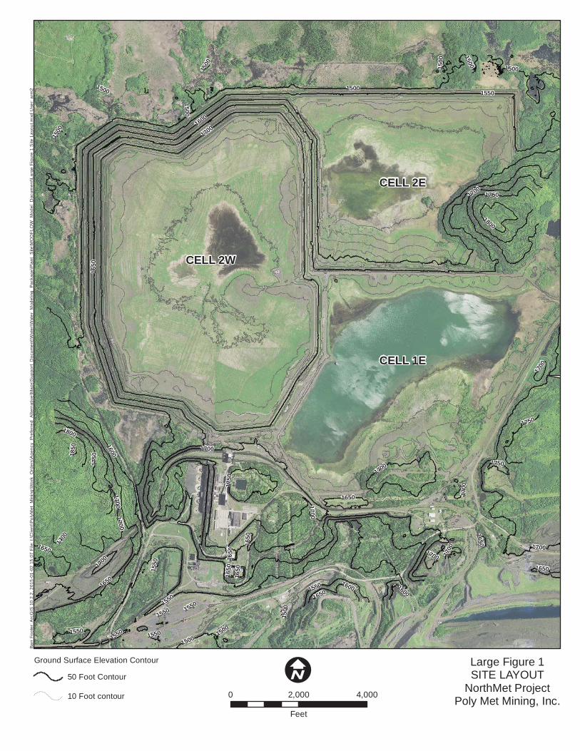
CELL 2W

CELL 2E

CELL 1E

1550

1600

150016

50

1700

1750

1800

1850

1750

1500

1500

1650

1500

1550

1700

1500

1700

1550

1700

1550

1700

17001700

1700

1550

1650

1500

1650

1700

16501550

1500

1500

1750

1800

1700

1650

1650

1500

1650

1750

1600

1550

1700

16001700

1550

1650

1750

1650

1500

1600

1700

15501650

1700

1500

Large Figure 1SITE LAYOUT

NorthMet ProjectPoly Met Mining, Inc.

Barr

Foo

ter:

Arc

GIS

10.

2.2,

201

5-01

-02

15:0

7 Fi

le: I

:\Clie

nt\P

olyM

et_M

inin

g\W

ork_

Ord

ers\

Age

ncy_

Pref

erre

d_A

ltern

ativ

e\M

aps\

Sup

port_

Doc

umen

t\Wat

er\W

ater

_Mod

elin

g_Pa

ckag

e\Pl

ant_

Site

\MO

DFL

OW

_Mod

el_D

ocum

ent\L

arge

Fig

ure

1 S

ite L

ayou

t.mxd

Use

r: ar

m2

I0 2,000 4,000

Feet

Ground Surface Elevation Contour

50 Foot Contour

10 Foot contour

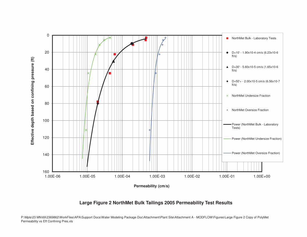
P:\Mpls\23 MN\69\2369862\WorkFiles\APA\Support Docs\Water Modeling Package Doc\Attachment\Plant Site\Attachment A - MODFLOW\Figures\Large Figure 2 Copy of PolyMet Permeability vs Eff Confining Pres.xls

0

20

40

60

80

100

120

140

1601.00E-06 1.00E-05 1.00E-04 1.00E-03 1.00E-02 1.00E-01 1.00E+00

Eff

ecti

ve d

epth

bas

ed o

n c

on

fin

ing

pre

ssu

re (

ft)

Permeability (cm/s)

Large Figure 2 NorthMet Bulk Tailings 2005 Permeability Test Results

NorthMet Bulk - Laboratory Tests

D=10' - 1.90x10-4 cm/s (6.23x10-6ft/s)

D=30' - 5.60x10-5 cm/s (1.65x10-6ft/s)

D=50'+ - 2.00x10-5 cm/s (6.56x10-7ft/s)

NorthMet Undersize Fraction

NorthMet Oversize Fraction

Power (NorthMet Bulk - LaboratoryTests)

Power (NorthMet Undersize Fraction)

Power (NorthMet Oversize Fraction)

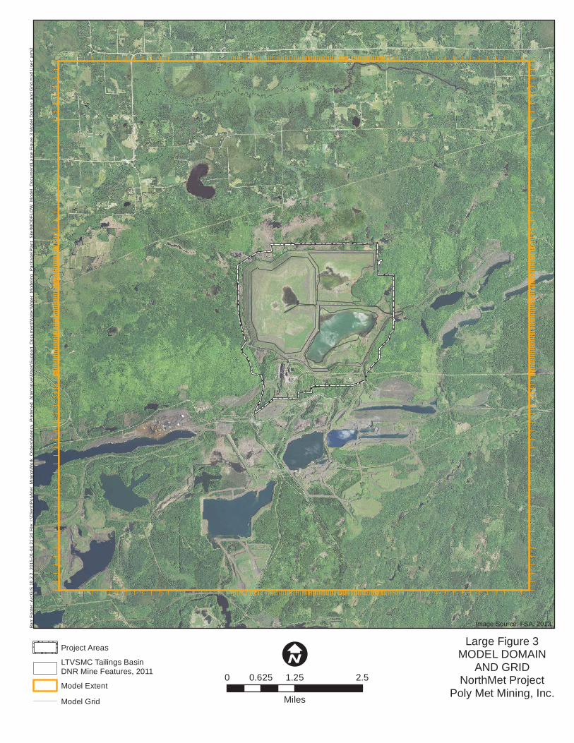
Barr

Foo

ter:

Arc

GIS

10.

2.2,

201

5-01

-04

21:2

4 Fi

le: I

:\Clie

nt\P

olyM

et_M

inin

g\W

ork_

Ord

ers\

Age

ncy_

Pref

erre

d_A

ltern

ativ

e\M

aps\

Sup

port_

Doc

umen

t\Wat

er\W

ater

_Mod

elin

g_Pa

ckag

e\Pl

ant_

Site

\MO

DFL

OW

_Mod

el_D

ocum

ent\L

arge

Fig

ure

3 M

odel

Dom

ain

and

Grid

.mxd

Use

r: ar

m2

Large Figure 3MODEL DOMAIN

AND GRIDNorthMet Project

Poly Met Mining, Inc.

Image Source: FSA, 2013.

Project Areas

LTVSMC Tailings BasinDNR Mine Features, 2011

Model Extent

Model Grid

I0 1.25 2.50.625

Miles

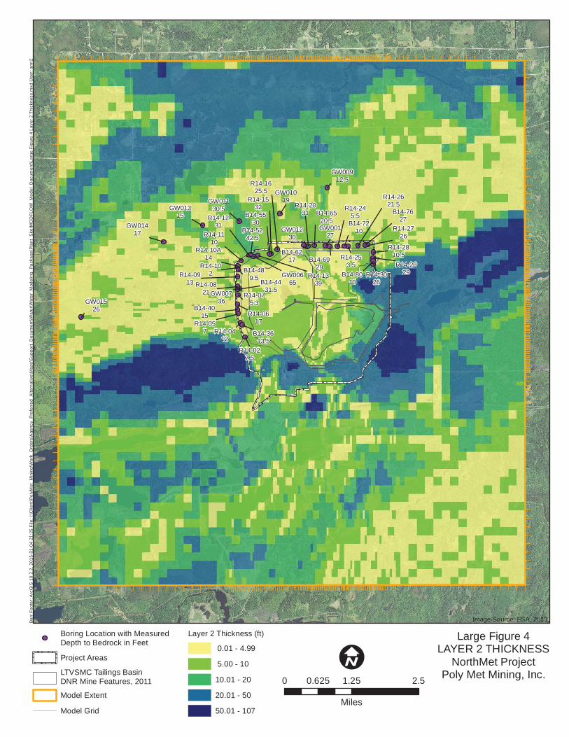
R14-102

R14-057

GW01526

GW01417

GW01315

GW01230

GW01019

GW00736

GW00127

B14-8010

B14-7627

B14-6929

B14-6217

B14-5530

B14-4015

R14-3026

R14-2929

R14-1532

R14-1110

R14-0913 R14-08

21

R14-0617

R14-0412

R14-027.5

GW01130.5

GW00912.5

B14-3613.5

R14-1625.5

R14-2621.5

R14-2810.5

B14-4431.5

B14-5242.5

B14-6520.5

R14-075.3

R14-10A14

R14-245.5

R14-253.5

B14-489.5

R14-1231

R14-1339

R14-2031

R14-2726

B14-7210

GW00665

Barr

Foo

ter:

Arc

GIS

10.

2.2,

201

5-01

-04

21:2

5 Fi

le: I

:\Clie

nt\P

olyM

et_M

inin

g\W

ork_

Ord

ers\

Age

ncy_

Pref

erre

d_A

ltern

ativ

e\M

aps\

Sup

port_

Doc

umen

t\Wat

er\W

ater

_Mod

elin

g_Pa

ckag

e\Pl

ant_

Site

\MO

DFL

OW

_Mod

el_D

ocum

ent\L

arge

Fig

ure

4 La

yer 2

Thi

ckne

ss.m

xd U

ser:

arm

2

Large Figure 4LAYER 2 THICKNESS

NorthMet ProjectPoly Met Mining, Inc.

Image Source: FSA, 2013.

Boring Location with MeasuredDepth to Bedrock in Feet

Project Areas

LTVSMC Tailings BasinDNR Mine Features, 2011

Model Extent

Model Grid

Layer 2 Thickness (ft)

0.01 - 4.99

5.00 - 10

10.01 - 20

20.01 - 50

50.01 - 107

I0 1.25 2.50.625

Miles

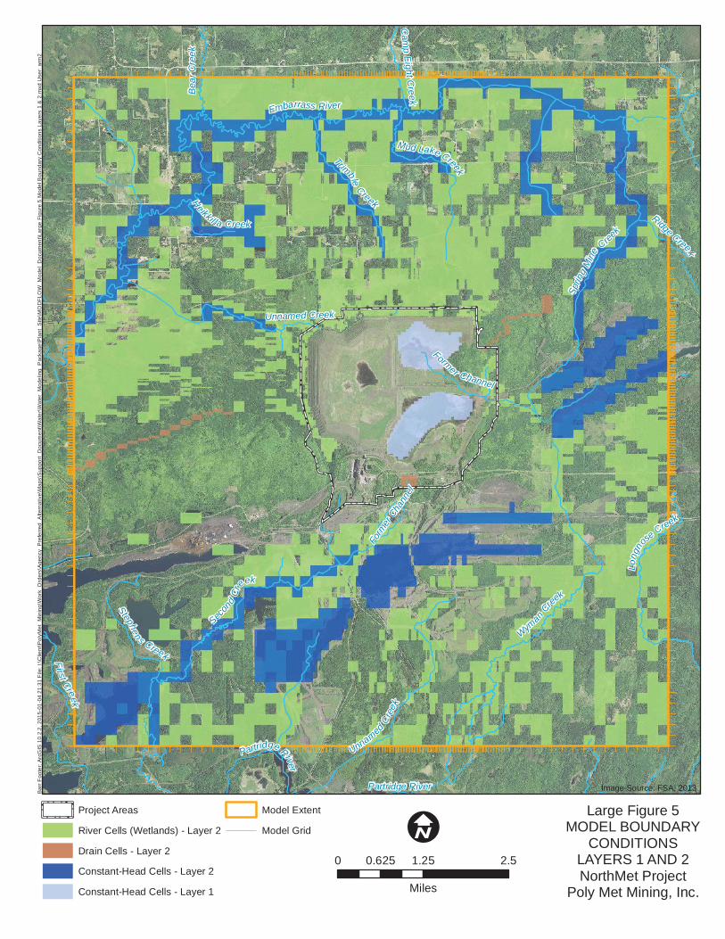
Embarrass River

Wyman Cree

k

Secon

dC

reek

First Creek

Sprin

gM

ine

Creek

UnnamedC

reek

Long

nose

Creek

Trimble

Creek

Mud Lake Creek

Bea

r Cre

ek

Ridge Creek

Stephens Creek

Cam

p Eight C

reek

Former Channel

Partridge River

H

eikkil la Creek

Form

er C

hann

el

Partridge River

Unnamed Creek

Bar

r Foo

ter:

Arc

GIS

10.

2.2,

201

5-01

-04

21:3

1 Fi

le: I

:\Clie

nt\P

olyM

et_M

inin

g\W

ork_

Ord

ers\

Age

ncy_

Pre

ferr

ed_A

ltern

ativ

e\M

aps\

Sup

port_

Doc

umen

t\Wat

er\W

ater

_Mod

elin

g_P

acka

ge\P

lant

_Site

\MO

DFL

OW

_Mod

el_D

ocum

ent\L

arge

Fig

ure

5 M

odel

Bou

ndar

y C

ondi

tions

Lay

ers

1 &

2.m

xd U

ser:

arm

2

Large Figure 5MODEL BOUNDARY

CONDITIONSLAYERS 1 AND 2NorthMet Project

Poly Met Mining, Inc.

Image Source: FSA, 2013.

Project Areas

River Cells (Wetlands) - Layer 2

Drain Cells - Layer 2

Constant-Head Cells - Layer 2

Constant-Head Cells - Layer 1

Model Extent

Model Grid I0 1.25 2.50.625

Miles

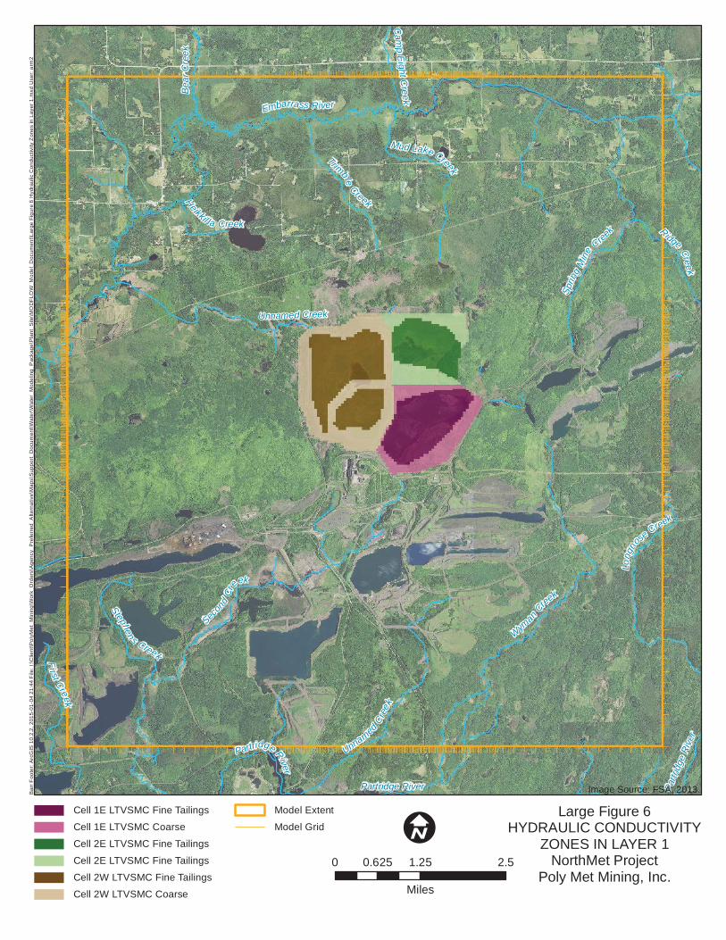
Embarrass River

Wyman Cree

k

Secon

dC

reek

First Creek

Sprin

gM

ine

Creek

UnnamedC

reek

Long

nose

Creek

Trimble

Creek

Mud Lake Creek

Ridge Creek

Bea

r Cre

ek

Stephens Creek

Cam

p Eight C

reek

Partr

idge

Riv

er

H

eikkil la Creek

Partridge River

Unnamed Creek

Partridge River

Bar

r Foo

ter:

Arc

GIS

10.

2.2,

201

5-01

-04

21:4

4 Fi

le: I

:\Clie

nt\P

olyM

et_M

inin

g\W

ork_

Ord

ers\

Age

ncy_

Pre

ferr

ed_A

ltern

ativ

e\M

aps\

Sup

port_

Doc

umen

t\Wat

er\W

ater

_Mod

elin

g_P

acka

ge\P

lant

_Site

\MO

DFL

OW

_Mod

el_D

ocum

ent\L

arge

Fig

ure

6 H

ydra

ulic

Con

duct

ivity

Zon

es in

Lay

er 1

.mxd

Use

r: ar

m2

Cell 1E LTVSMC Fine Tailings

Cell 1E LTVSMC Coarse

Cell 2E LTVSMC Fine Tailings

Cell 2E LTVSMC Fine Tailings

Cell 2W LTVSMC Fine Tailings

Cell 2W LTVSMC Coarse

Model Extent

Model GridLarge Figure 6

HYDRAULIC CONDUCTIVITYZONES IN LAYER 1

NorthMet ProjectPoly Met Mining, Inc.

Image Source: FSA, 2013.

I0 1.25 2.50.625

Miles

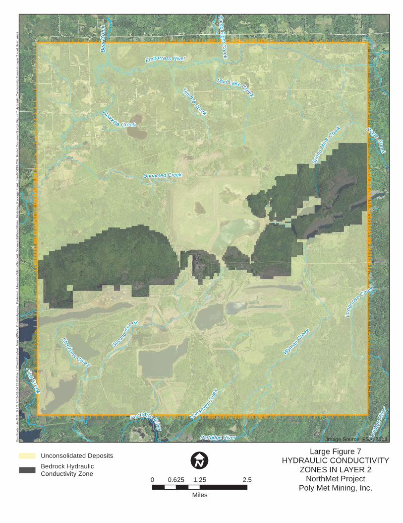
Embarrass River

Wyman Cree

k

Secon

dC

reek

First Creek

Sprin

gM

ine

Creek

UnnamedC

reek

Long

nose

Creek

Trimble

Creek

Mud Lake Creek

Ridge Creek

Bea

r Cre

ek

Stephens Creek

Cam

p Eight C

reek

Partr

idge

Riv

er

H

eikkil la Creek

Partridge River

Unnamed Creek

Partridge River

Bar

r Foo

ter:

Arc

GIS

10.

2.2,

201

5-01

-04

22:0

5 Fi

le: I

:\Clie

nt\P

olyM

et_M

inin

g\W

ork_

Ord

ers\

Age

ncy_

Pre

ferr

ed_A

ltern

ativ

e\M

aps\

Sup

port_

Doc

umen

t\Wat

er\W

ater

_Mod

elin

g_P

acka

ge\P

lant

_Site

\MO

DFL

OW

_Mod

el_D

ocum

ent\L

arge

Fig

ure

7 H

ydra

ulic

Con

duct

ivity

Zon

es in

Lay

er 2

.mxd

Use

r: ar

m2

Unconsolidated Deposits

Bedrock HydraulicConductivity Zone

Large Figure 7HYDRAULIC CONDUCTIVITY

ZONES IN LAYER 2NorthMet Project

Poly Met Mining, Inc.

Image Source: FSA, 2013.

I0 1.25 2.50.625

Miles

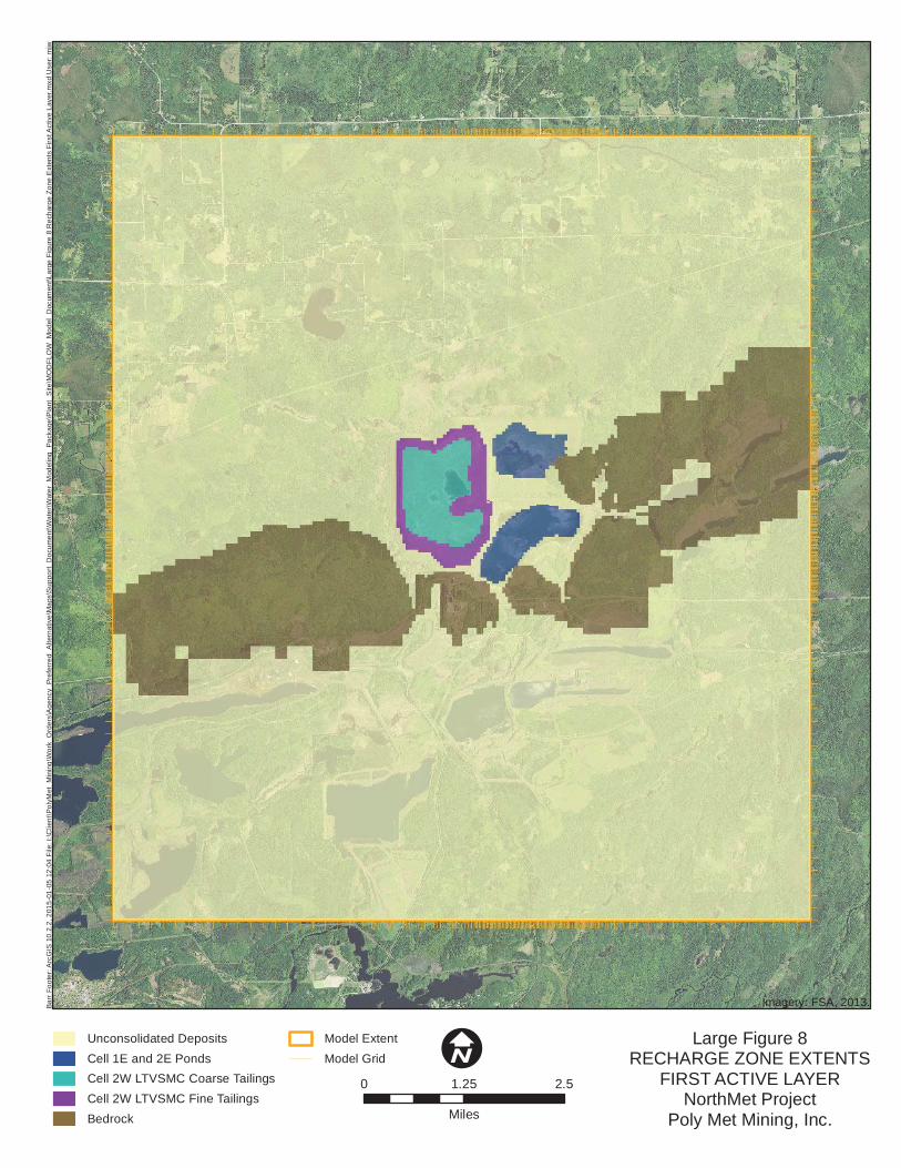
Barr

Foo

ter:

Arc

GIS

10.

2.2,

201

5-01

-05

12:0

4 Fi

le: I

:\Clie

nt\P

olyM

et_M

inin

g\W

ork_

Ord

ers\

Age

ncy_

Pref

erre

d_A

ltern

ativ

e\M

aps\

Sup

port_

Doc

umen

t\Wat

er\W

ater

_Mod

elin

g_Pa

ckag

e\Pl

ant_

Site

\MO

DFL

OW

_Mod

el_D

ocum

ent\L

arge

Fig

ure

8 R

echa

rge

Zone

Ext

ents

Firs

t Act

ive

Laye

r.mxd

Use

r: m

jw

Unconsolidated DepositsCell 1E and 2E PondsCell 2W LTVSMC Coarse TailingsCell 2W LTVSMC Fine TailingsBedrock

Model ExtentModel Grid

Large Figure 8RECHARGE ZONE EXTENTS

FIRST ACTIVE LAYERNorthMet Project

Poly Met Mining, Inc.

Imagery: FSA, 2013.

I0 1.25 2.5

Miles

!(

!(

!(

!(

!(

!(

!(

!(

!(

!(

!(

!(

!(

!(

!(

!(

!(

!<<

!<<

!<!!<!!<

!<<

!<<

!<<

!<

!<!<

!<

!<

!<

!<

!!<

!!<

!!<

!!<

!!<

!!<

!!<

!!<!!<

!!<!!<

!!<!!<!!< !!<!(!!<!!< !!<!( !(!( !( !!<

!<

!<

!<

!<!<

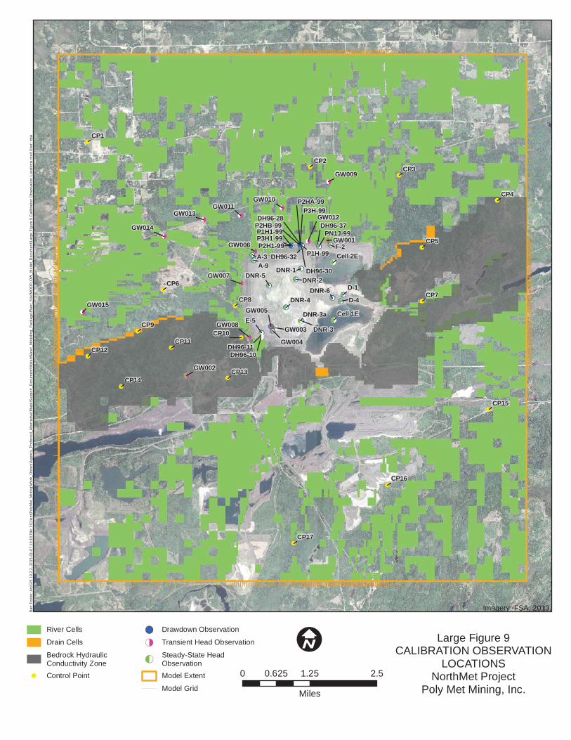
GW015

GW014

GW013 GW012GW011

GW010

GW009

GW008

GW007

GW006

GW005

GW004

GW003

GW002

GW001 CP5

CP7

CP2

CP9

CP8

CP6

CP4

CP3

CP1

CP17

CP16

CP15

CP14CP13

CP12CP11

CP10

Cell 1E

Cell 2E

DH96-10DH96-11

F-2A-3A-9

D-1

D-4

DNR-5

DNR-6DNR-4

DNR-2DNR-1

P3H-99

P1H-99DH96-32

P2HA-99

DH96-37DH96-28

DH96-30

P1H1-99

P2H1-99

P2HB-99

P3H1-99PN1J-99

DNR-3a

DNR-3E-5

Bar

r Fo

oter

: Arc

GIS

10.

2.2,

201

5-01

-07

10:1

9 Fi

le: I

:\Clie

nt\P

olyM

et_M

inin

g\W

ork_

Ord

ers\

Age

ncy_

Pre

ferr

ed_A

ltern

ativ

e\M

aps\

Sup

port_

Doc

umen

t\Wat

er\W

ater

_Mod

elin

g_P

acka

ge\P

lant

_Site

\MO

DFL

OW

_Mod

el_D

ocum

ent\L

arge

Fig

ure

9 C

alib

ratio

n O

bser

vatio

n Lo

catio

ns.m

xd U

ser:

mjw

River Cells

Drain Cells

Bedrock HydraulicConductivity ZoneControl Point

!( Drawdown Observation

< Transient Head Observation

!<(Steady-State HeadObservationModel Extent

Model Grid

Large Figure 9CALIBRATION OBSERVATION

LOCATIONSNorthMet Project

Poly Met Mining, Inc.

Imagery: FSA, 2013.

I0 1.25 2.50.625

Miles

!.

!.

!.

!.

!.

!.

!.

!.

!.

!.

!.

!.

!.!.!.

!.!. !. !.

!.

!.

!.

!.!.

!.

!.!.

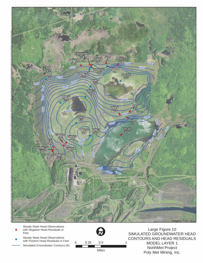
Cell 1E-0.01

Cell 2E0.01

GW004-4.1

GW005-6.8

DH96-11-23.1

DH96-10-24.1

GW003-14.5

F-2-5.8

A-3-9.2

A-921.1

D-4-2.7

DNR-45.3

P1H1-99-4.0

DNR-522.1

DNR-325.1

DNR-210.9

DNR-121.7

DNR-3a19.1

PN1J-997.7

P1H-99-1.6

DH96-302.5

DNR-6-12.3

DH96-37-10.6

E-5-4.6

D-1-17.7

P2HA-99-3.8

DH96-3210.2

1570

'

1530'

1560'

1580'

1550

'15

40'

1590'

1610'

1600'

1620'

1630

'

1640'

1650

'

1520'1510'

1660'

1660'

1630'

1660'

1520'

1640

'

1510'

1580'

1650'

1640

'

1650

'

1650

'1620'

1640'1650'

1640'

1610'

1520'

Barr

Foo

ter:

Arc

GIS

10.

2.2,

201

5-01

-07

10:1

1 Fi

le: I

:\Clie

nt\P

olyM

et_M

inin

g\W

ork_

Ord

ers\

Agen

cy_P

refe

rred_

Alte

rnat

ive\

Map

s\Su

ppor

t_D

ocum

ent\W

ater

\Wat

er_M

odel

ing_

Pack

age\

Pla

nt_S

ite\M

OD

FLO

W_M

odel

_Doc

umen

t\Lar

ge F

igur

e 10

Sim

ulat

ed G

roun

dwat

er H

ead

Con

tour

s an

d H

ead

Res

idua

ls in

Lay

er.m

xd U

ser:

kam

2

!.

Steady-State Head Observationswith Negative Head Residuals inFeet

!.Steady-State Head Observationswith Positive Head Residuals in FeetSimulated Groundwater Contours (ft)

Large Figure 10SIMULATED GROUNDWATER HEADCONTOURS AND HEAD RESIDUALS

MODEL LAYER 1NorthMet Project

Poly Met Mining, Inc.

Imagery: FSA, 2013.

I0 0.5 10.25

Miles

!.

!.

!.

!.

!.

!.

!.

!.

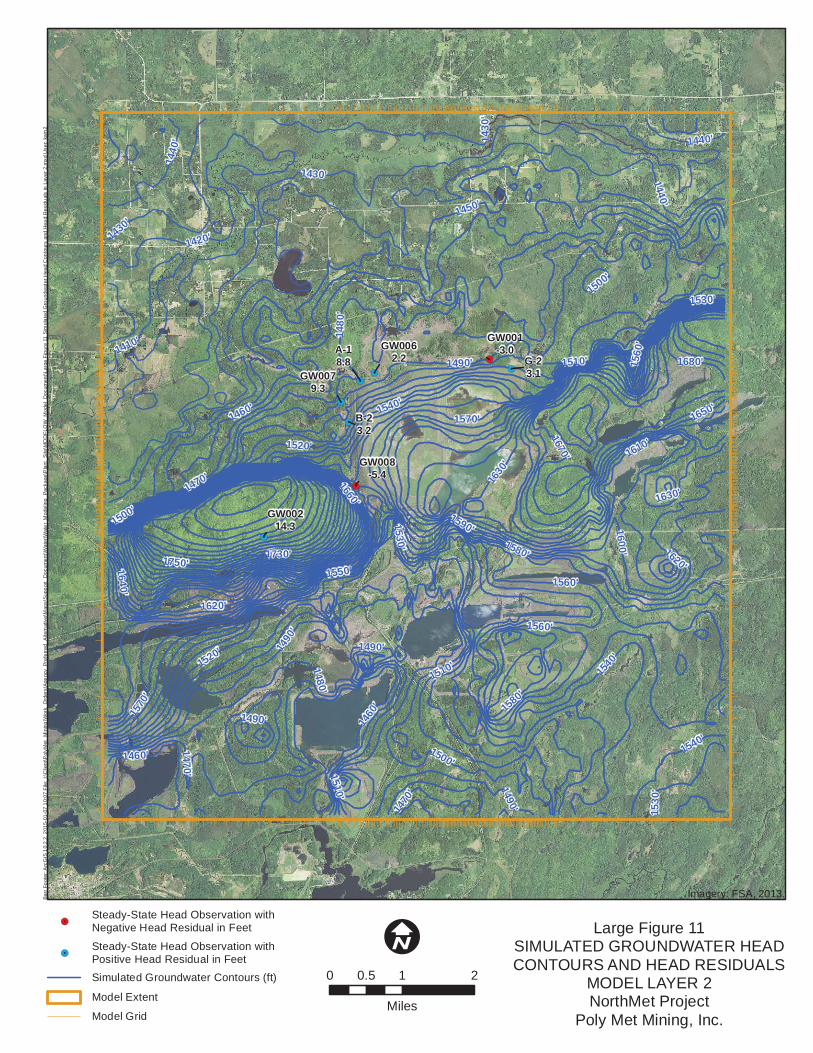
GW001-3.0

GW0079.3

GW0062.2

GW008-5.4

GW00214.3

G-23.1

B-23.2

A-18.8

1440'

1450'

1460'

1470'

1480

'

1490'

1500'

1510'

1520'

1530'

1540'

1550'

1560

'

1430'

1570'

1580'

1590' 1600'

1610'

1620'

1630

'

1640'

1650'

1660'

1670'

1680'

1420'

1730'1750'

1410'

1540'

1440

'

1580'

1500'

1460'

1470'

1490

'

1440'

1510'

1560'

1470

'

1570

'

1500'

1560'

1490'

1530'

1490'

1490'

1630'

1460

'

1520'

1540

'

1480'14

30'

1620'

1430'

1510'15

30'

Barr

Foo

ter:

Arc

GIS

10.

2.2,

201

5-01

-07

10:0

7 Fi

le: I

:\Clie

nt\P

olyM

et_M

inin

g\W

ork_

Ord

ers\

Agen

cy_P

refe

rred_

Alte

rnat

ive\

Map

s\Su

ppor

t_D

ocum

ent\W

ater

\Wat

er_M

odel

ing_

Pack

age\

Pla

nt_S

ite\M

OD

FLO

W_M

odel

_Doc

umen

t\Lar

ge F

igur

e 11

Sim

ulat

ed G

roun

dwat

er H

ead

Con

tour

s an

d H

ead

Res

idua

ls in

Lay

er 2

.mxd

Use

r: ka

m2

!.Steady-State Head Observation withNegative Head Residual in Feet

!.Steady-State Head Observation withPositive Head Residual in FeetSimulated Groundwater Contours (ft)

Model Extent

Model Grid

Large Figure 11SIMULATED GROUNDWATER HEADCONTOURS AND HEAD RESIDUALS

MODEL LAYER 2NorthMet Project

Poly Met Mining, Inc.

Imagery: FSA, 2013.

I0 1 20.5

Miles

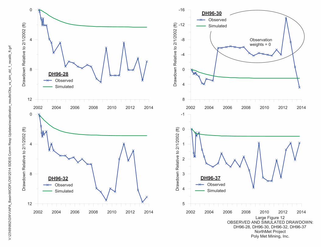
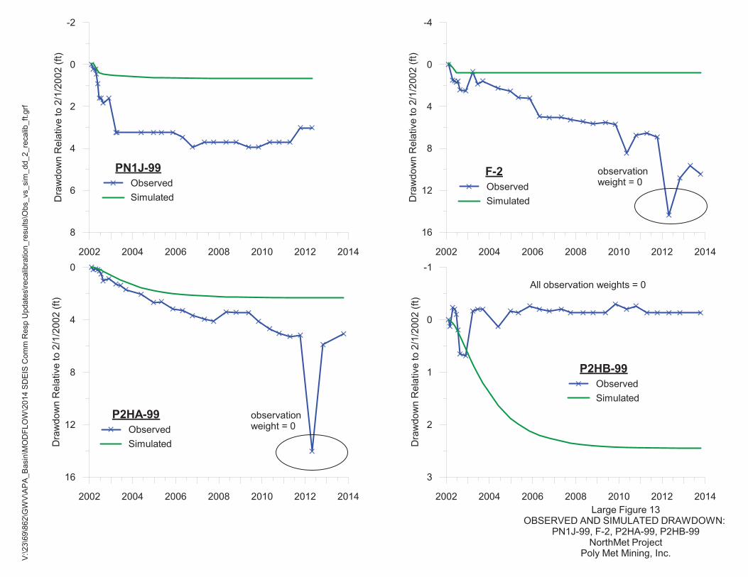
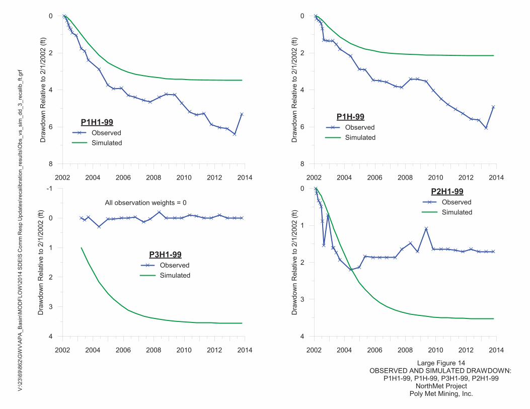
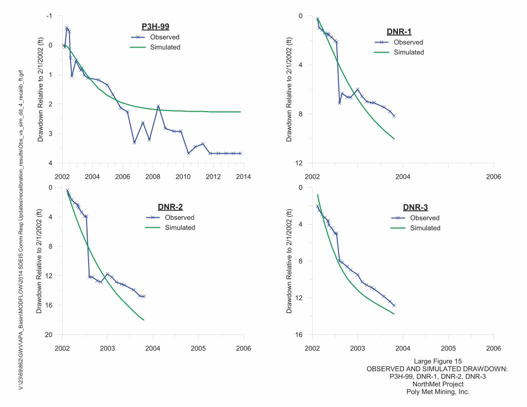
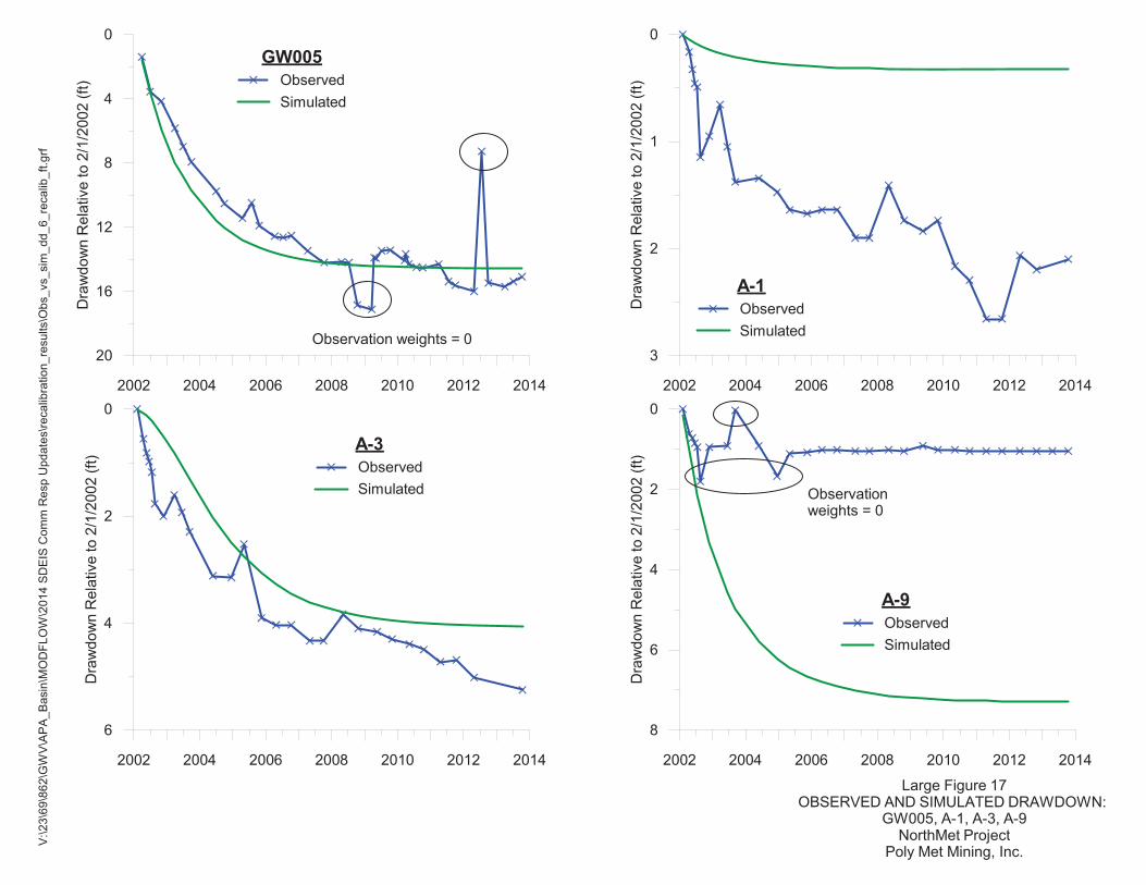
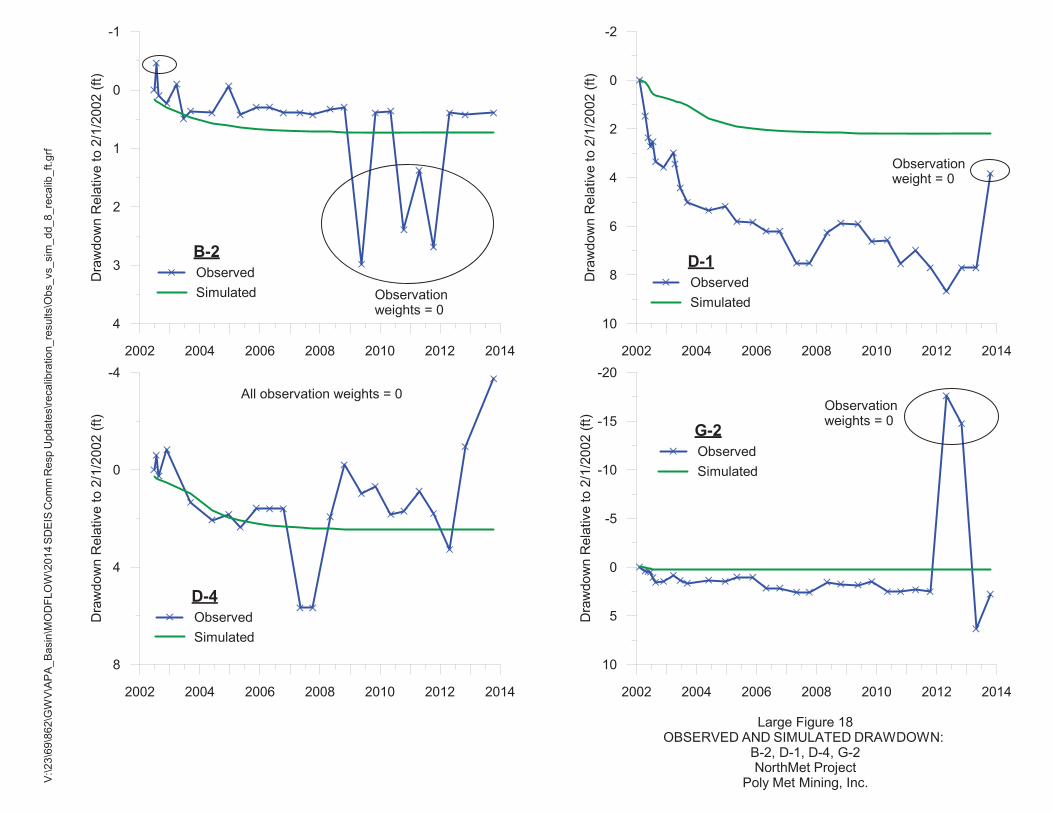
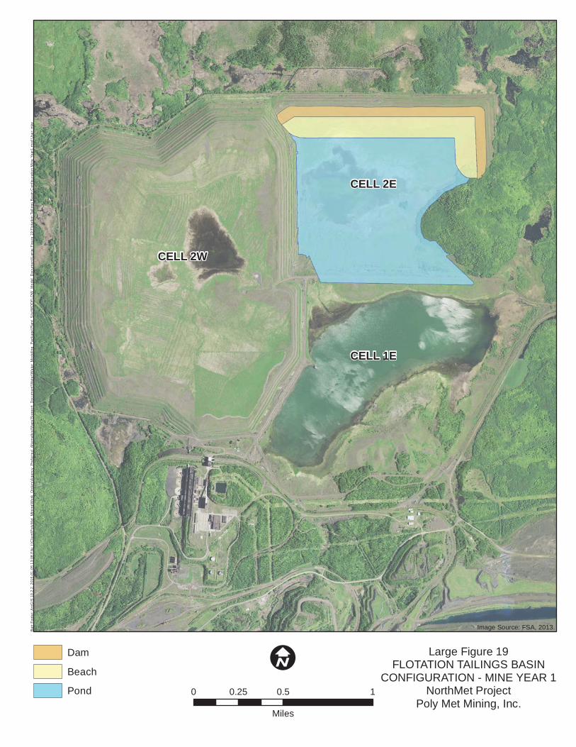
CELL 2W

CELL 2E

CELL 1E

Bar

r Fo

oter

: Arc

GIS

10.

2.2,

201

5-01

-05

13:0

8 Fi

le: I

:\Clie

nt\P

olyM

et_M

inin

g\W

ork_

Ord

ers\

Age

ncy_

Pre

ferr

ed_A

ltern

ativ

e\M

aps\

Sup

port_

Doc

umen

t\Wat

er\W

ater

_Mod

elin

g_P

acka

ge\P

lant

_Site

\MO

DFL

OW

_Mod

el_D

ocum

ent\L

arge

Fig

ure

19 F

lota

tion

Taili

ngs

Bas

in C

onfig

urat

ion

Min

e Ye

ar1.

mxd

Use

r: m

jw

Large Figure 19FLOTATION TAILINGS BASIN

CONFIGURATION - MINE YEAR 1NorthMet Project

Poly Met Mining, Inc.

Dam

Beach

Pond

I0 0.5 10.25

Miles

Image Source: FSA, 2013.

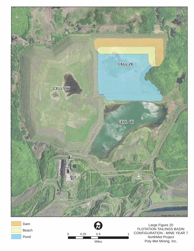
CELL 2W

CELL 2E

CELL 1E

Barr

Foo

ter:

Arc

GIS

10.

2.2,

201

5-01

-07

10:0

2 Fi

le: I

:\Clie

nt\P

olyM

et_M

inin

g\W

ork_

Ord

ers\

Agen

cy_P

refe

rred_

Alte

rnat

ive\

Map

s\Su

ppor

t_D

ocum

ent\W

ater

\Wat

er_M

odel

ing_

Pack

age\

Pla

nt_S

ite\M

OD

FLO

W_M

odel

_Doc

umen

t\Lar

ge F

igur

e 20

Flo

tatio

n Ta

ilings

Bas

in C

onfig

urat

ion

Min

e Ye

ar7.

mxd

Use

r: ka

m2

Large Figure 20FLOTATION TAILINGS BASIN

CONFIGURATION - MINE YEAR 7NorthMet Project

Poly Met Mining, Inc.

Dam

Beach

Pond

I0 0.5 10.25

Miles

Image Source: FSA, 2013.

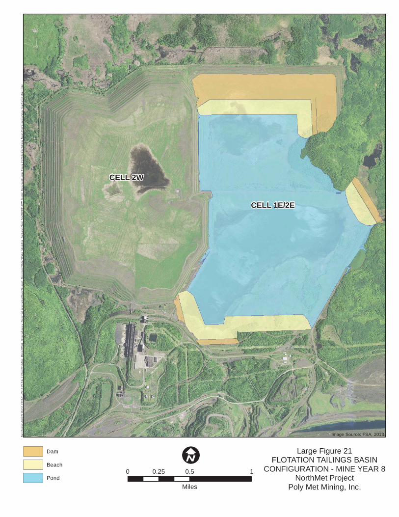
CELL 2W

CELL 1E/2E

Bar

r Fo

oter

: Arc

GIS

10.

2.2,

201

5-01

-05

13:2

5 Fi

le: I

:\Clie

nt\P

olyM

et_M

inin

g\W

ork_

Ord

ers\

Age

ncy_

Pre

ferr

ed_A

ltern

ativ

e\M

aps\

Sup

port_

Doc

umen

t\Wat

er\W

ater

_Mod

elin

g_P

acka

ge\P

lant

_Site

\MO

DFL

OW

_Mod

el_D

ocum

ent\L

arge

Fig

ure

21 F

lota

tion

Taili

ngs

Bas

in C

onfig

urat

ion

Min

e Ye

ar8.

mxd

Use

r: m

jw

Large Figure 21FLOTATION TAILINGS BASIN

CONFIGURATION - MINE YEAR 8NorthMet Project

Poly Met Mining, Inc.

Dam

Beach

Pond

Image Source: FSA, 2013.

I0 0.5 10.25

Miles

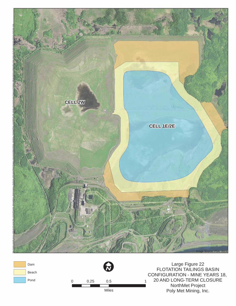
CELL 2W

CELL 1E/2E

Bar

r Fo

oter

: Arc

GIS

10.

2.2,

201

5-01

-05

14:0

2 Fi

le: I

:\Clie

nt\P

olyM

et_M

inin

g\W

ork_

Ord

ers\

Age

ncy_

Pre

ferr

ed_A

ltern

ativ

e\M

aps\

Sup

port_

Doc

umen

t\Wat

er\W

ater

_Mod

elin

g_P

acka

ge\P

lant

_Site

\MO

DFL

OW

_Mod

el_D

ocum

ent\L

arge

Fig

ure

22 F

lota

tion

Taili

ngs

Bas

in C

onfig

urat

ion

Min

e Ye

ars

18 2

0 an

d Lo

ng-te

rm C

losu

re.m

xd U

ser:

mjw

Large Figure 22FLOTATION TAILINGS BASIN

CONFIGURATION - MINE YEARS 18, 20 AND LONG-TERM CLOSURE

NorthMet ProjectPoly Met Mining, Inc.

Dam

Beach

Pond

I0 0.5 10.25

Miles

Image Source: FSA, 2013.

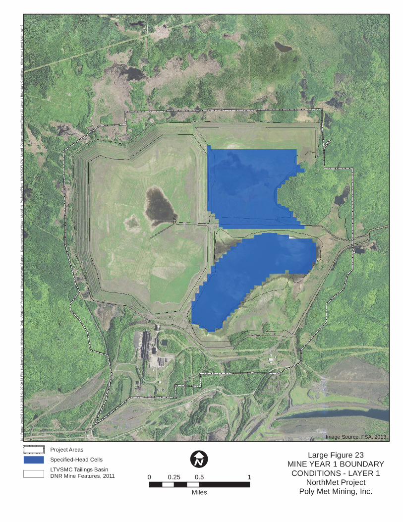
Barr

Foot

er: A

rcG

IS 1

0.2.

2, 2

015-

01-0

7 09

:58

File

: I:\C

lient

\Pol

yMet

_Min

ing\

Wor

k_O

rder

s\A

genc

y_Pr

efer

red_

Alte

rnat

ive\

Map

s\S

uppo

rt_D

ocum

ent\W

ater

\Wat

er_M

odel

ing_

Pac

kage

\Pla

nt_S

ite\M

OD

FLO

W_M

odel

_Doc

umen

t\Lar

ge F

igur

e 23

Lay

er 1

Bou

ndar

y C

ondi

tions

- M

ine

Year

1.m

xd U

ser:

kam

2

Project Areas

Specified-Head Cells

LTVSMC Tailings BasinDNR Mine Features, 2011

Large Figure 23MINE YEAR 1 BOUNDARYCONDITIONS - LAYER 1

NorthMet ProjectPoly Met Mining, Inc.

Image Source: FSA, 2013.

I0 0.5 10.25

Miles

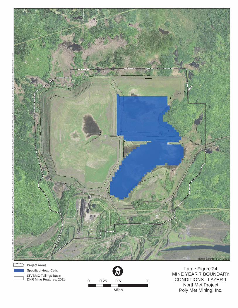
Barr

Foo

ter:

Arc

GIS

10.

2.2,

201

5-01

-07

09:5

3 Fi

le: I

:\Clie

nt\P

olyM

et_M

inin

g\W

ork_

Ord

ers\

Agen

cy_P

refe

rred_

Alte

rnat

ive\

Map

s\Su

ppor

t_D

ocum

ent\W

ater

\Wat

er_M

odel

ing_

Pack

age\

Pla

nt_S

ite\M

OD

FLO

W_M

odel

_Doc

umen

t\Lar

ge F

igur

e 24

Lay

er 1

Bou

ndar

y C

ondi

tions

- M

ine

Year

7.m

xd U

ser:

kam

2

Project AreasSpecified-Head CellsLTVSMC Tailings BasinDNR Mine Features, 2011

Large Figure 24MINE YEAR 7 BOUNDARYCONDITIONS - LAYER 1

NorthMet ProjectPoly Met Mining, Inc.

Image Source: FSA, 2013.

I0 0.5 10.25

Miles

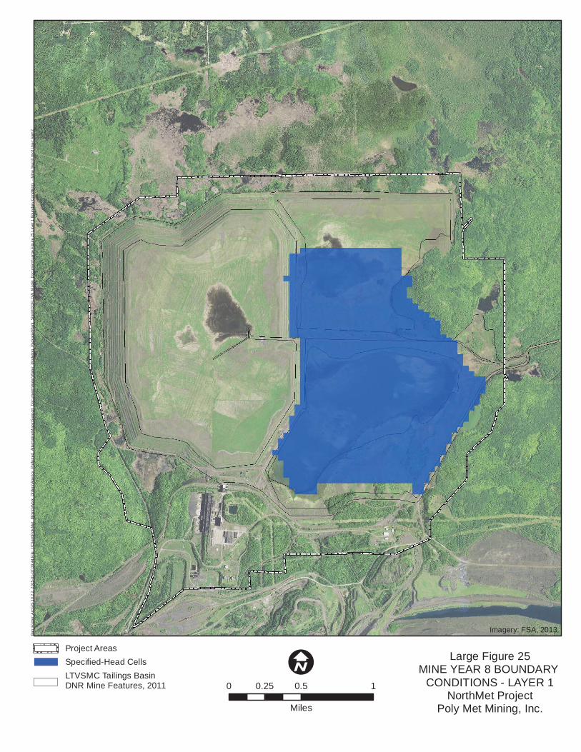
Barr

Foo

ter:

Arc

GIS

10.

2.2,

201

5-01

-07

09:4

4 Fi

le: I

:\Clie

nt\P

olyM

et_M

inin

g\W

ork_

Ord

ers\

Agen

cy_P

refe

rred_

Alte

rnat

ive\

Map

s\Su

ppor

t_D

ocum

ent\W

ater

\Wat

er_M

odel

ing_

Pack

age\

Pla

nt_S

ite\M

OD

FLO

W_M

odel

_Doc

umen

t\Lar

ge F

igur

e 25

Lay

er 1

Bou

ndar

y C

ondi

tions

- M

ine

Year

8.m

xd U

ser:

kam

2

Project AreasSpecified-Head CellsLTVSMC Tailings BasinDNR Mine Features, 2011

Large Figure 25MINE YEAR 8 BOUNDARY

CONDITIONS - LAYER 1NorthMet Project

Poly Met Mining, Inc.

Imagery: FSA, 2013.

I0 0.5 10.25

Miles

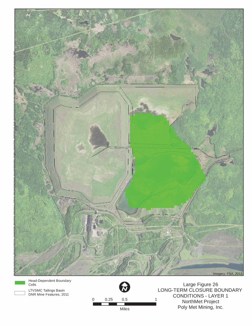
Barr

Foo

ter:

Arc

GIS

10.

2.2,

201

5-01

-07

09:4

7 Fi

le: I

:\Clie

nt\P

olyM

et_M

inin

g\W

ork_

Ord

ers\

Agen

cy_P

refe

rred_

Alte

rnat

ive\

Map

s\Su

ppor

t_D

ocum

ent\W

ater

\Wat

er_M

odel

ing_

Pack

age\

Pla

nt_S

ite\M

OD

FLO

W_M

odel

_Doc

umen

t\Lar

ge F

igur

e 26

Lay

er 1

Bou

ndar

y C

ondi

tions

- L

ong-

term

Clo

sure

.mxd

Use

r: ka

m2

Head-Dependent BoundaryCells

LTVSMC Tailings BasinDNR Mine Features, 2011

Large Figure 26LONG-TERM CLOSURE BOUNDARY

CONDITIONS - LAYER 1NorthMet Project

Poly Met Mining, Inc.

Imagery: FSA, 2013.

I0 0.5 10.25

Miles

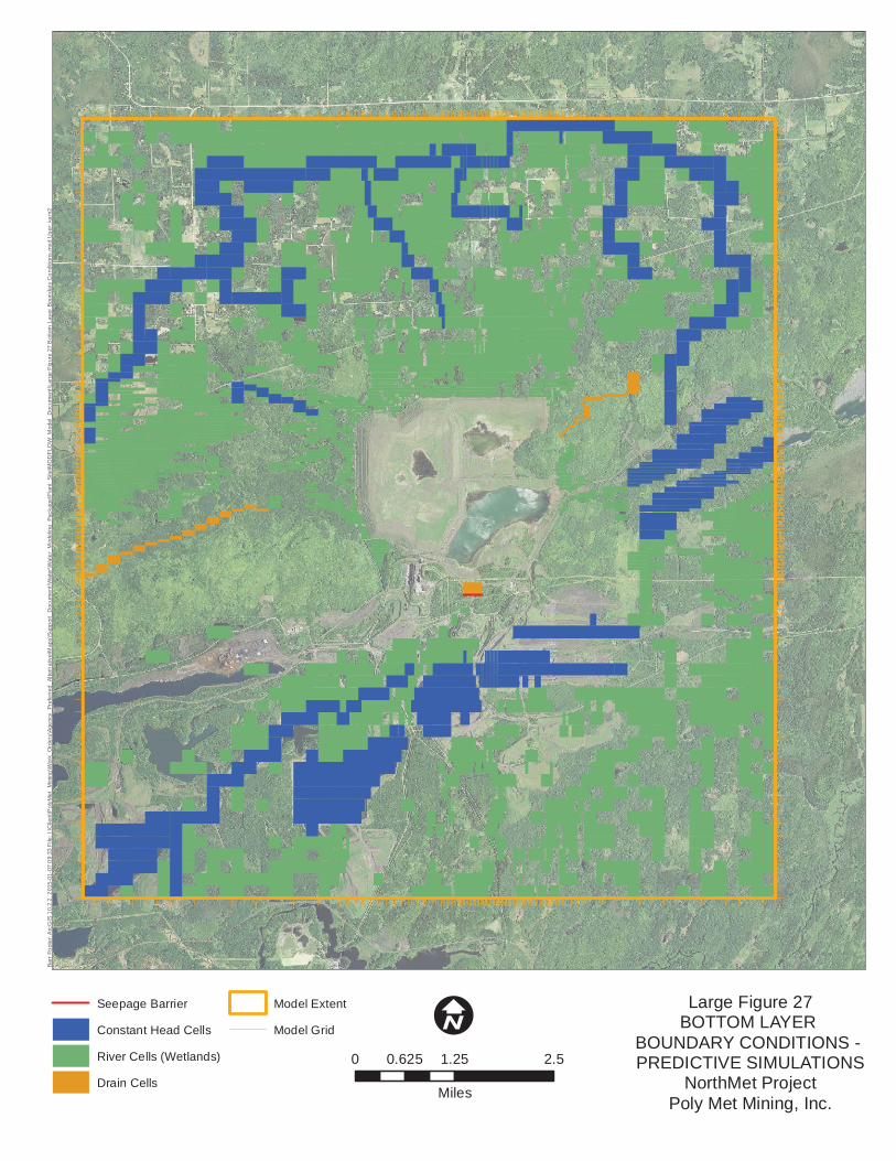
Seepage Barrier

Constant Head Cells

River Cells (Wetlands)

Drain Cells

Model Extent

Model Grid

Large Figure 27BOTTOM LAYER

BOUNDARY CONDITIONS - PREDICTIVE SIMULATIONS

NorthMet ProjectPoly Met Mining, Inc.

Barr

Foo

ter:

Arc

GIS

10.

2.2,

201

5-01

-07

09:3

3 Fi

le: I

:\Clie

nt\P

olyM

et_M

inin

g\W

ork_

Ord

ers\

Agen

cy_P

refe

rred_

Alte

rnat

ive\

Map

s\Su

ppor

t_D

ocum

ent\W

ater

\Wat

er_M

odel

ing_

Pack

age\

Pla

nt_S

ite\M

OD

FLO

W_M

odel

_Doc

umen

t\Lar

ge F

igur

e 27

Bot

tom

Lay

er B

ound

ary

Con

ditio

ns.m

xd U

ser:

kam

2

I0 1.25 2.50.625

Miles