A GROUNDWATER MODEL TO DETERMINE THE AREA WITHIN THE UPPER BIGBLUE NATURAL RESOURCES DISTRICT WHERE GROUNDWATER PUMPING

HAS THE POTENTIAL TO INCREASE FLOW FROM THE PLATTE RIVER TO THEUNDERLYING AQUIFER BY AT LEAST 10 PERCENT OF THE VOLUME PUMPED

OVER A 50-YEAR PERIOD

Prepared ByR.J. Bitner, P.E.

Upper Big Blue Natural Resources DistrictSeptember 2005

EMSI is an acronym for “Environmental Modeling Systems, Inc.”1

GMS is an acronym for “Groundwater Modeling System”.2

COHYST is an acronym for “ Cooperative Hydrology Study”. 3

ACKNOWLEDGMENTS

The following persons provided assistance with inputs and reviews that were incorporated intothe model and final report:

Courtney Hemenway, P.E., Hemenway Groundwater Engineering, Inc., provided a peer review ofthe model development, model inputs, model application, and report to ensure that thesecomponents are developed in accordance with acceptable standards.

Duane Woodward, Hydrologist, Central Platte Natural Resources District, reviewed the modeland inputs for consistency with COHYST standards. Duane also assisted with evaluatingrecent river bed conductance data that was incorporated into the model.

Steve Peterson, Hydrologist, U.S. Geological Survey, assisted with implementation of the EMSI 1

GMS modeling techniques. 2

Jim Cannia, Nebraska Department of Natural Resources, reviewed the model and model inputsregarding suitability for determining hydrologic connectivity of streams with the aquifer.

Marie Krausnick, Upper Big Blue Natural Resources District, provided assistance with GISmapping.

Xun Hong Chen, Ph.D. and Mark Burhach, Ph.D., University of Nebraska Conservation andSurvey Division, provided Geoprobe electric logging, permeameter testing, and pumptests to estimate aquifer hydraulic conductivity and river bed conductance on the PlatteRiver and Big Blue River.

Larry Cast, Geologist, reviewed test hole and irrigation well drilling logs to determine geologicand hydrologic properties of the layers used to define the aquifer.

Rich Kern, P.E., Hydrologist / Programmer, Nebraska Department of Natural Resources,provided computer programming of utilities to assist with database management,grouping geologic layer parameters, retrieving data from the DNR databases, and analysisof GMS - MODFLOW outputs.

COHYST Modelers , developed the COHYST Eastern Regional groundwater model from which3

this sub-regional model is derived.

AUTHORIZATION

The groundwater model discussed in this report was commissioned by the Upper Big BlueNatural Resources District for the purpose of estimating the location of areas within the NaturalResources District that have the potential to be hydrologically connected to base-flow streams. The groundwater model and modeling results, shown in this report, have been presented to theNatural Resources District Board, and have been approved for submittal to the NebraskaDepartment of Natural Resources.

TABLE OF CONTENTS

INTRODUCTION . . . . . . . . . . . . . . . . . . . . . . . . . . . . . . . . . . . . . . . . . . . . . . . . . . . . . . . . . . . . . 1

PURPOSE . . . . . . . . . . . . . . . . . . . . . . . . . . . . . . . . . . . . . . . . . . . . . . . . . . . . . . . . . . . . . . . . . . . 1

CONCEPTUAL MODEL . . . . . . . . . . . . . . . . . . . . . . . . . . . . . . . . . . . . . . . . . . . . . . . . . . . . . . . 1

GEOLOGIC AND HYDROSTRATIGRAPHIC UNITS . . . . . . . . . . . . . . . . . . . . . . . . . . . . . . . 4

MODEL DESCRIPTION . . . . . . . . . . . . . . . . . . . . . . . . . . . . . . . . . . . . . . . . . . . . . . . . . . . . . . . . 5Model Grid . . . . . . . . . . . . . . . . . . . . . . . . . . . . . . . . . . . . . . . . . . . . . . . . . . . . . . . . . . . . . 5Modules . . . . . . . . . . . . . . . . . . . . . . . . . . . . . . . . . . . . . . . . . . . . . . . . . . . . . . . . . . . . . . . 5

River Module . . . . . . . . . . . . . . . . . . . . . . . . . . . . . . . . . . . . . . . . . . . . . . . . . . . . . 5Well Module . . . . . . . . . . . . . . . . . . . . . . . . . . . . . . . . . . . . . . . . . . . . . . . . . . . . . 6Recharge Module . . . . . . . . . . . . . . . . . . . . . . . . . . . . . . . . . . . . . . . . . . . . . . . . . . 7Evapotranspiration Module . . . . . . . . . . . . . . . . . . . . . . . . . . . . . . . . . . . . . . . . . . 7

Boundary Conditions . . . . . . . . . . . . . . . . . . . . . . . . . . . . . . . . . . . . . . . . . . . . . . . . . . . . . 8Model Flow Simulation . . . . . . . . . . . . . . . . . . . . . . . . . . . . . . . . . . . . . . . . . . . . . . . . . . . 9Flow Equation Solver . . . . . . . . . . . . . . . . . . . . . . . . . . . . . . . . . . . . . . . . . . . . . . . . . . . . 9Aquifer Characteristics . . . . . . . . . . . . . . . . . . . . . . . . . . . . . . . . . . . . . . . . . . . . . . . . . . 10

xHydraulic Conductivity K . . . . . . . . . . . . . . . . . . . . . . . . . . . . . . . . . . . . . . . . . . 10Anisotropic Ratios . . . . . . . . . . . . . . . . . . . . . . . . . . . . . . . . . . . . . . . . . . . . . . . . 11

ySpecific Yield S . . . . . . . . . . . . . . . . . . . . . . . . . . . . . . . . . . . . . . . . . . . . . . . . . 11Specific Storage Ss . . . . . . . . . . . . . . . . . . . . . . . . . . . . . . . . . . . . . . . . . . . . . . . 11

PRE-DEVELOPMENT PERIOD . . . . . . . . . . . . . . . . . . . . . . . . . . . . . . . . . . . . . . . . . . . . . . . . 12Mean Difference . . . . . . . . . . . . . . . . . . . . . . . . . . . . . . . . . . . . . . . . . . . . . . . . . . . . . . . 13Mean Absolute Difference . . . . . . . . . . . . . . . . . . . . . . . . . . . . . . . . . . . . . . . . . . . . . . . . 13Root Mean Square Difference . . . . . . . . . . . . . . . . . . . . . . . . . . . . . . . . . . . . . . . . . . . . . 13

PRE-DEVELOPMENT MODEL - WITHOUT PUMPING . . . . . . . . . . . . . . . . . . . . . . . . . . . . 14

HYDROLOGICALLY CONNECTED AREA . . . . . . . . . . . . . . . . . . . . . . . . . . . . . . . . . . . . . . 1510% / 50-Year Boundary Determination . . . . . . . . . . . . . . . . . . . . . . . . . . . . . . . . . . . . . 18

S. M. Peterson, Groundwater Flow Model of the Eastern Model Unit of the Nebraska Cooperative4

Hydrology Study (COHYST) Area, 2005.

Nebraska Department of Natural Resources, Proposed Rule pursuant to Neb. Rev. Stat. §46-713.5

1

INTRODUCTION

This report discusses development and application of a groundwater model for a region

that lies within the boundary of the Cooperative Hydrology Study (COHYST) eastern regional

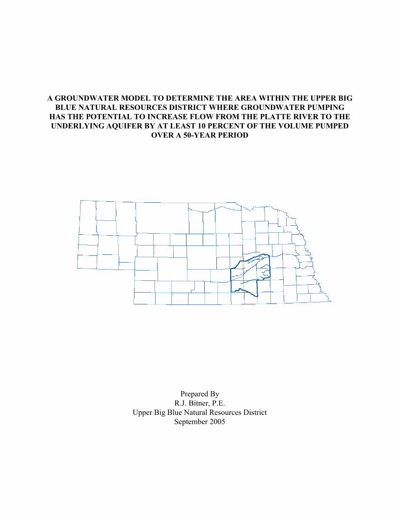
groundwater model in Nebraska. The geographic area modeled is shown on Figure 1 and4

includes all, or portions of, Platte, Polk, York, Nance, Merrick, Hamilton, Clay, Nuckolls,

Howard, Hall, and Adams Counties. The modeled area overlays portions of the Upper Big Blue,

Central Platte, and Little Blue Natural Resources Districts. The total land surface within the

model boundary is approximately 7,520 square miles (4.8 million acres).

PURPOSE

The purpose of this model is to provide a method for calculating the potential increase in

the rate of flow from the Platte River to the underlying aquifer due to groundwater pumping near

the Platte River within the Upper Big Blue Natural Resources District. The model is used to

define a boundary encompassing the area within which a well pumping groundwater could

increase flow from the Platte River to the underlying aquifer by an amount equal to, or greater

than, 10 percent of the volume pumped over a period of 50 years. For purposes of determining

whether or not a river basin is fully appropriated , the Nebraska Department of Natural5

Resources considers that wells within the 10 percent / 50-year boundary are hydrologically

connected to the river.

CONCEPTUAL MODEL

The model boundaries are defined with a series of fixed flow arcs that specify flow into or

out of the model, depending upon the direction and slope of the groundwater gradient at the

boundary. The Platte River is defined with a series of river arcs which specify the river bed

conductance, river bed thickness, and river stage. The model cells intersected by the river arcs

are defined by the model as a series of point source river cells, each with its own conductance

value. The model cells intersected by the fixed flow boundary arcs are defined by the model as a

series of wells that are either source (injection) or sink (withdrawal), depending on whether the

2

Xun Hong Chen, River Bed Conductance Studies - West Fork Big Blue River and Platte River in6

Nebraska, University of Nebraska Conservation and Survey Division, 2005.

3

boundary flow is into or out of the model at that point. The amount of river to aquifer flow

induced by pumping is tested with a single well, which is moved from cell to cell parallel to the

Platte River, at varying distances from the river. Other streams within the model boundary, such

as the Big Blue River and its tributaries, including the West Fork Big Blue River, Lincoln Creek,

and Beaver Creek, are not included in the model. The bed conductances of these rivers and

streams are very low, approximately 0.0079 ft /day, and have minimal connectivity to the2

underlying aquifer and the Platte River. Areal sources and sinks included in this model are6

recharge from precipitation, and evapotranspiration from rooted plants located in wet meadows

near the Platte River. The model geology is represented by five unconfined layers. The

numerical flow model is based on the following basic assumptions:

• At the scale in which this model is constructed, flow in the aquifer obeys Darcy’s Law

and mass and energy are conserved.

• Since the modeled fluid is groundwater, having a temperature in the range of 50 degrees

Fahrenheit, the density and viscosity of water are constant over time and space.

• Parameters are uniform within each cell, and represent an estimate of their average value

within the cell.

• The interchange of water between the aquifer and Platte River can be adequately

simulated as one-dimensional flow through a discrete streambed layer. This

conceptualization is appropriate over the scale at which this model is constructed.

• Hydraulic conductivity in the horizontal plane is isotropic; however, hydraulic

conductivity in the vertical direction is not equal to hydraulic conductivity in the

horizontal direction. The horizontal to vertical anisotropic ratio is assigned a value of 10

(i.e. horizontal hydraulic conductivity is ten times greater than vertical hydraulic

conductivity), unless otherwise noted.

J. C. Cannia, D. Woodward, L. Cast, and R. L. Luckey, Cooperative Hydrology Study COHYST7

Hydrostratigraphic Units and Aquifer Characterization Report, November 2004.

See geoprobe electric logs shown in Appendix B8

4

GEOLOGIC AND HYDROSTRATIGRAPHIC UNITS

The model has five unconfined geologic layers. The layer definitions are consistent with

those documented in the COHYST aquifer characterization report . The model layers consist7

primarily of Quaternary deposits of Pleistocene alluvium, Pleistocene and Holocene loess,

Holocene dune sand, and Holocene valley fill. Valley fill deposits are found along the Platte

River and consist of gravel, sand, and silt. Alluvial deposits, which typically support high

capacity wells, are found throughout the model area. In topographic bedrock highs these deposits

are generally thinner, and produce lower yielding wells. Loess deposits are found throughout the

model area, and the thickest deposits are located along the Platte River bluffs. The deposits

become thinner as they approach the Platte River north of the loess bluffs. The Platte River bed

contains a low permeability loess layer at about 10 to 20 feet below the current streambed

surface . The bedrock formation at the bottom of Layer 5 consists of shale, chalk, limestone,8

siltstone, and sandstone of Cretaceous age. These bedrock materials transmit very little water,

and for modeling purposes are considered to be impermeable.

The model layers are numbered 1 through 5. Unit 1 is the top layer, and Unit 5 is the

bottom layer. The layers used in this model are described as follows:

• Layer 1 Top layer consisting of upper Quaternary age silt and clay with some sand

and gravel

• Layer 2 Middle Quaternary age sand and gravel

• Layer 3 Lower Quaternary age silt and clay with some sand and gravel

• Layer 4 Upper Tertiary age silt and clay with some sand and gravel

• Layer 5 Middle Tertiary age sand and gravel underlain with bedrock materials

consisting of shale, chalk, limestone, siltstone, and sandstone

M. G. McDonald and A.W. Harbaugh, Modular Three-Dimensional Finite-Difference9

Groundwater Flow Model, U.S. Geological Survey, 1984.

Groundwater Modeling System (GMS), Environmental Modeling Systems, Inc. (EMSI), Park City,10

Utah.

5

MODEL DESCRIPTION

The groundwater model is a three-dimensional finite difference computer model

developed around the MODFLOW , Version 2000, groundwater modeling software enclosed9

within EMSI GMS , Version 5.1. The GMS software includes a pre-processor to read input data10

and place it in the model according to MODFLOW format requirements. GMS also does some

post-processing of output in both graphical and numerical forms. The units of measure used in

this model include feet for linear measure, days for time, feet per day for velocity, cubic feet for

volume, and cubic feet per day for flow rate.

Model Grid

The model grid has 120,330 cells per layer. Each cell measures 1,320 feet per side, and

covers an area of approximately 40 acres. Model feature locations are geo-referenced in the

horizontal plane to the Nebraska State Plane Coordinate System, NAD 83 - feet. Top and bottom

elevations of each layer are referenced to USGS mean sea level datum.

Modules

The MODFLOW software is modular in the sense that various modules (packages) can be

activated for any particular modeling situation. The modules used in this model include river,

well, recharge, and evapotranspiration.

River Module

The Platte River is simulated in this model as a series of arcs, connected at their upstream

and downstream ends at nodes, with a combined length of 87.8 miles. Attributes associated with

the arcs and nodes specify the river bed conductance, bottom of river bed elevation, and river

ystage. The hydrologic properties (K, S ) of model cells identified as river cells (cells crossed by

river arcs), and located in Layer 1, are adjusted to match the hydrologic properties of the

underlying cell in Layer 2. In this way there is a direct connection of the Platte River bed to the

aquifer, and the only limitation on inter-connectivity between the river bed and underlying

Documentation of a Computer Program to Simulate Stream-Aquifer Relations Using a Modular,11

Finite Difference, Groundwater Flow Model, U.S. Geological Survey, Open-File Report 88-729,

1989.

6

aquifer is river bed conductance. River bed conductance is a function of river bed length, width,

bed thickness, and hydraulic conductivity. MODFLOW uses the following equation to11

calculate bed conductance:

EQ. 1 C = (k x L x W) / M

For each river arc “n”:

nC = streambed conductance (ft /d/ft)2

vnk = vertical hydraulic conductivity of the streambed (ft/d)

nL = length of the streambed (ft)

nW = width of streambed (ft)

nM = thickness of streambed (ft)

For this model, the value of river bed conductance at each river arc is set at the same value as

used in the COHYST Eastern Regional Model, except where detailed testing indicates the value

should be different. The values established by testing were determined based on geoprobe and

permeameter tests conducted by the University of Nebraska Conservation and Survey Division.

Geoprobe electric logs, hydraulic conductivities, and bed conductance calculations are shown in

Appendix B of this report. Platte River bed conductances used in this model are set at 11 ft /d/ft2

in reaches where testing is completed. River bed conductances in the remaining reaches vary

from 20 ft /d/ft to 30 ft /d/ft.2 2

Well Module

The potential increase in induced flow from the Platte River to the underlying aquifer,

due to groundwater pumping near the Platte River, is tested with this model by placing a

simulated pumping well at alternate cell locations, operating the model for a 50-year period at

each location, and calculating the change in the water budget when compared with the baseline

condition. The initial baseline condition is simulated with no pumping well.

For these simulations, pumping is assumed to be from Layer 2, the volume of water

7

pumped is set at 160 acre-feet per year, and the pumping rate is set to be continuous at 19,094.79

cubic feet per day. This volume of groundwater is approximately the average amount of water

pumped in one year to irrigate a quarter section of crop. A gravity irrigated system would pump

slightly more volume on average, and a pivot irrigated system would pump slightly less volume

on average, based on the District’s records of irrigation water use. Although irrigation systems

typically operate at a higher pumping rate, are operated on an intermittent pumping schedule, and

only operate for a few months per year, a continuous lower pumping rate is used to simplify the

modeling process. The volume of water pumped per year would be the same with either

continuous or transient pumping schedules. The continuous pumping schedule is not expected to

give significantly different results than a transient pumping schedule would yield. Some

comparisons of continuous and transient pumping were made to confirm this conclusion.

Recharge Module

Recharge is modeled as an areal source of inflow to the aquifer, and includes the amount

of precipitation that percolates from the surface through Layer 1 into Layer 2. The recharge rate

used in this model, in feet per day, is interpolated from the COHYST Eastern Model, pre-

development period, scatter point data set. The scatter point file is derived from the COHYST

EMU model and interpolated to this model’s 2-dimensional grid. The 2D data set is imported to

the MODFLOW model recharge array. The recharge point of application option is set to the

highest active layer at each grid cell. For this model, the minimum recharge rate is 0.000222 feet

per day (0.97 inches per year), and the maximum rate is 0.000557 feet per day (2.44 inches per

year). The mean rate is 0.000222 feet per day (0.972 inches per year). The recharge rate is held

constant throughout the modeled time period, and does not vary from stress period to stress

period.

Evapotranspiration Module

Evapotranspiration (ET) is modeled as the amount of groundwater extracted from the

aquifer by rooted vegetation, and then evaporated from the plant canopy to the atmosphere

external from the model. For this model ET is considered to be an areal sink; i.e., outflow from

the model space. The ET rate data set used in this model is interpolated from the COHYST

Eastern Model pre-development data set. A scatter point file is produced from the COHYST

8

EMU model and interpolated to this model’s 2-dimensional grid. The 2D data set is then

imported to the MODFLOW model ET array. The point of ET withdrawal is the top of Layer 1,

and the extinction depth is set at a specified depth (nominally 7 feet) below the top of Layer 1.

For this sub-regional model, the minimum ET rate is 0.00 feet per day, and the maximum rate is

0.002993 feet per day (13.1 inches per year). The rate of evapotranspiration is held constant

throughout the modeled time period, and does not vary from stress period to stress period.

Wetland areas, mostly located near the Platte River, are treated as groundwater sinks,

where groundwater can be removed from the model space by plant evapotranspiration. The

evapotranspiration rate, extinction depth, and active ET layer are interpolated to the model 2D

grid from COHYST EMU scatter point data sets. Areas that have potential for significant

evapotranspiration are selected using 1997 land use mapping data for wetlands (Dappen and

Tooze, 2001), and also by defining areas where the depth to groundwater is on average 7 feet or

less below land surface, according to USGS long-term depth to water data (U.S. Geological Survey

National Water Information System, 1999).

Boundary Conditions

The model is bounded vertically by land surface at the top of Layer 1 and bedrock at the

bottom of Layer 5. The model is bounded horizontally by fixed flow boundaries. A fixed flow

boundary is a boundary where the flow is specified prior to the simulation and held constant

throughout the simulation (McDonald and Harbaugh, 1988). At fixed flow boundaries the

simulated water level can change, but flow across the boundary does not change. The northern

model boundary is aligned with the Loup River and the southern boundary is aligned with the

Little Blue River and southern boundary of Adams County. The eastern model boundary is

aligned with the eastern boundaries of York and Polk Counties, and the western boundary is

aligned with the western boundaries of Hall and Adams Counties, as shown on Figure 1. The

rate of flow through each model boundary, in cubic feet per day, is calculated using the Darcy

Equation.

9

EQ. 2

For each boundary arc “n”

nQ = fixed rate of flow through the boundary, ft /d3

nk = weighted horizontal hydraulic conductivity, ft/d

ni = gradient of the 1950 groundwater surface perpendicular to the boundary flow

plane, ft/ft

nA = cross sectional area of the flow plane at the boundary, ft2

Each layer’s thickness determines the relative weight given to each layer’s hydraulic

conductivity for this calculation. The calculated boundary flow is distributed evenly over the

saturated thickness between the groundwater level and the base of the aquifer at each boundary

arc. Appendix A contains calculations and supporting documents used to compute boundary

fixed flows. A boundary flow is not computed for Layer 1, since it is a silty clay layer generally

representing the unsaturated zone which overlays the saturated zone.

Model Flow Simulation

The MODFLOW software has several packages (BCF, LPF, and HUF) available for

calculating conductance coefficients and groundwater storage parameters to be used in the finite-

difference equations that calculate flow between cells. The Layer Property Flow (LPF) package

is selected as the internal flow calculation methodology for this model. The LPF package reads

input data for hydraulic conductivity and global top and bottom elevation data for each cell

(layer). Transmissivity is calculated for each cell at the beginning of each iteration of the flow

equation matrix solution process. The LPF package calculates leakance between layers using the

x zvertical hydraulic conductivity, based on estimated anisotropic ratio K /K , and distance between

nodes obtained from global elevation data.

Flow Equation Solver

The MODFLOW software has several linear differential equation “solver” packages

(SIP1, PCG2, SCR1, and GMG) available. For this model, the pre-conditioned conjugate-

P. Concus, G. H. Golub, and D. P. O’Leary, A Generalized Conjugate Gradient for the Numerical12

Solution of Elliptical Partial Differential Equations, Academic Press, 1976.

J. C. Cannia, D. Woodward, L. Cast, and R. L. Luckey, Cooperative Hydrology Study COHYST13

Hydrostratigraphic Units and Aquifer Characterization Report, November 2004.

E. C. Reed and R. Piskin, unpublished report, University of Nebraska Conservation and Survey14

Division.

10

gradient (PCG2) package is selected to solve the linear finite difference equation matrix. For a12

transient groundwater model, the solution matrix is expressed as shown in EQ. 3, where [A] is

the coefficient matrix, [x] is a vector of hydraulic heads, and [b] is a vector of defined flows,

associated with head-dependent boundary conditions and storage terms at each grid cell.

EQ. 3

The matrix is solved iteratively until both head-change and residual convergence criteria are met.

The convergence criteria are too large if the global groundwater flow budget discrepancy is

unacceptably large. In general, a global budget discrepancy less than one percent is considered

acceptable. Convergence criteria for this model, specified in the input options for the PCG2

module, are 0.5 foot for heads and 10.0 ft /d for flow residual. The iteration parameters are not3

specified, but rather are calculated internally.

Aquifer Characteristics

Aquifer properties are input for each layer, including horizontal hydraulic conductivity

x x z z(K ), vertical anisotropic ratio (K /K ) or vertical hydraulic conductivity K , horizontal

x y s yanisotropic ratio (K /K ), Specific Storage (S ), and specific yield (S ). The procedures used to

estimate parameter values for each layer are described in the COHYST hydrostratigraphic Units

Characterization Report .13

xHydraulic Conductivity K

Test well logs, interpreted by Reed and Piskin , are the basis for horizontal hydraulic14

conductivity values used in this groundwater model and the COHYST eastern regional model.

The interpreted values for each layer are weighted according to layer thickness, and the weighted

xaverage value of K is then determined for each model layer at each test well location. The

R. Kern, Nebraska Cooperative Hydrology Study Computer Program Documentation GeoParam -15

Hydraulic Conductivity from Well Logs, Nebraska Department of Natural Resources.

Personal communication with Xun Hong Chen, University of Nebraska, Conservation and Survey16

Division.

11

process used to weight the values is written in a computer code called Geoparm . A 2D data set15

is then created by interpolating the computed values. The 2D data set is then used to set the

MODFLOW array of values for each layer.

Anisotropic Ratios

x zAs described previously in this report, the vertical anisotropic ratio, K /K , is estimated

to be 10.0 for all layers at each grid cell, unless pump testing indicates a different ratio, and the

x yhorizontal anisotropic ratio, K /K , is estimated to be 1.0.

ySpecific Yield S

Data compiled by USGS, and summarized by Reed and Piskin, is the basis for specific

yield values used in this groundwater model and the COHYST eastern regional model. As

discussed in the Hydrostratigraphic Units Report, specific yield values are interpreted for each

layer material classification. The interpreted values are then weighted using the Geoparm

program to establish specific yield for each model layer at each test well location. The computed

values are then interpolated to the model’s 2D grid for each model layer. The 2D data sets are

then used to set the MODFLOW array values for each layer.

Specific Storage Ss

All layers in this model are considered to be unconfined; however, the LPF simulation

options available in MODFLOW are either confined or convertible. The convertible option is

selected for all layers, and the specific storage for all layers, except Layer 1, is set to 2.1e ; this-3

value is based on discussions with UNL Conservation and Survey and takes into account low16

potential for changes in aquifer storage due to height of overburden or changes in hydraulic head.

The specific storage for Layer 1 is set to 0.16, the estimated specific yield, since this layer is

always unconfined, and cannot be converted to confined.

Specific storage is the volume of water per unit volume of confined saturated aquifer that

is absorbed, or expelled, due to changes in pressure within the aquifer. Overburden tends to

12

consolidate the aquifer (reduce storage volume), and hydraulic pressure head tends to offset

consolidation (increase storage volume).

Storativity for a confined layer is equal to the product of specific storage and layer

thickness. Storativity for an unconfined layer is equal to the specific yield plus the product of

groundwater depth and specific storage.

PRE-DEVELOPMENT PERIOD

Geologic and hydrogeologic layer parameters used in this model are derived from

calibrated COHYST eastern regional model (EMU) data. The EMU was calibrated for the pre-

groundwater development period by varying and adjusting evapotranspiration, recharge,

hydraulic conductivity, properties at horizontal flow boundaries, and streambed conductances.

For this model the evapotranspiration, recharge and horizontal hydraulic conductivity are

interpolated from EMU scatter point files. Streambed conductances and vertical hydraulic

conductivities are adjusted at some locations based on recent testing conducted by the University

of Nebraska Conservation and Survey. Fixed flows at boundaries are computed for each

boundary arc as previously described. Observed water levels, measured between 1946 and 1955,

are used to establish the starting head values.

Observed water levels used to establish starting heads are from a period of relatively

stable conditions. Observation points were selected as being representative of pre-groundwater

development, and only the most reliable data within 4-mile by 4-mile grid cells were selected (by

COHYST modelers) for EMU calibration. This selection process prevents a cluster of closely

spaced observation wells from dominating the calibration process. After screening values in all

of the 4 by 4-mile cells, a few points that appeared to have large errors in location or land-surface

elevation were excluded from the calibration data set. The starting heads file for this model is

based on a sub-set of the EMU calibration data set that contains 209 of the observation points.

The ability of this model to represent a 50-year period of pre-groundwater development

conditions is evaluated by comparing the percent discrepancy in global groundwater flow budget,

as well as the mean difference, mean absolute difference, and root mean square of the differences

between observed pre-development groundwater levels at the beginning and end of a 50-year

computer run without well development.

13

Mean Difference

The mean difference (MD) of observed and simulated water levels is defined in EQ.4.

0 sThe variable h is the observed water level and h is the simulated water level at each of the n

observation points. The mean difference is used here as a measure of overall bias in calibration,

and as such should be close to zero at calibration.

EQ.4

Mean Absolute Difference

The mean absolute difference (MAD) of observed and simulated water levels is defined

in EQ.5. The MAD is used here to evaluate the overall model calibration, since positive and

negative differences do not cancel each other. All differences are given an equal weight, so a few

measurements with large differences will not dominate the result.

EQ.5

MODFLOW calculates the water level changes as draw-downs, therefore positive changes are

declines and negative changes are rises.

Root Mean Square Difference

The root mean square difference (RMSD), also referred to as the quadratic mean, is

defined in EQ. 6. This statistic is the standard deviation of the differences between observed

groundwater levels and groundwater levels produced by the model, for the pre-development

period. Assuming that the differences between observed and modeled water levels are normally

distributed about the mean difference, the standard deviation gives a measure for determining the

range within which the differences can be expected to occur. Statistically, 68.27% of the

differences are expected to occur within MD ± RMSD, and 95.45% of the differences are

expected to occur within MD ± (2)(RMSD).

EQ. 6

14

PRE-DEVELOPMENT MODEL - WITHOUT PUMPING

Starting heads for the pre-development model are obtained by interpolating the observed

pre-development water levels to the model 2D grid, which is then imported to the MODFLOW

model starting head data set. The observation data points are also imported to the model so that

heads computed by the model can be compared to the starting heads for the purpose of evaluating

groundwater level changes over the 50-year period. Figures 2 and 3 show the locations of water

level observation points, water level contours, and statistical variation at each observation point

for the starting heads and 50-year model run. Statistical variations are shown in 10 feet

increments; green indicates variation from 0 to 10 feet, yellow indicates variation from 10 to 20

feet, and red indicates variation from 20 to 30 feet. If the indicator is above the line, the

computed water level is higher than observed, and if the indicator is below the line the computed

water level is lower than observed at that observation point. The mean difference between

observed and interpolated water levels, for both starting heads and 50-year model run, is 0.240

feet, the mean absolute difference is 1.376 feet, and the root mean square difference is 2.235 feet.

Statistically it can be expected that approximately 95% of the differences between observed and

computed water levels will occur within ± 2.235 feet of the mean difference.

The global groundwater inflow and outflow budgets, without well development, are

shown in Tables 1 and 2 for the 50-year model run.

TABLE 1

MODEL INFLOW VOLUMETRIC BUDGET

Inflow From Inflow Volume

(KAF)

Inflow Rate

(KAF / Yr.)

Percent of Inflow

(%)

Storage 19,088 382 52.1

Fixed Flow Boundary 2,324 46 6.4

Platte River 4,388 88 12.0

Recharge 10,781 216 29.5

Total Inflow 36,580 732 100

15

TABLE 2

MODEL OUTFLOW VOLUMETRIC BUDGET

Outflow From Outflow Volume

(KAF)

Outflow Rate

(KAF / Yr.)

Percent of Outflow

(%)

Storage 22,196 444 60.7

Fixed Flow Boundary 5,599 112 15.3

Platte River 106 2 0.3

Evapotranspiration 8,681 174 23.7

Total Outflow 36,582 732 100

For the 50-year no well development scenario, the model calculates flow from the Platte

River to the underlying aquifer at an average rate of 86 acre-feet per year within the model

boundaries. This river to aquifer flow, without pumping, is the baseline for computing induced

river to aquifer flow due to groundwater pumping. The global groundwater flow budget

discrepancy is less than 0.01 percent.

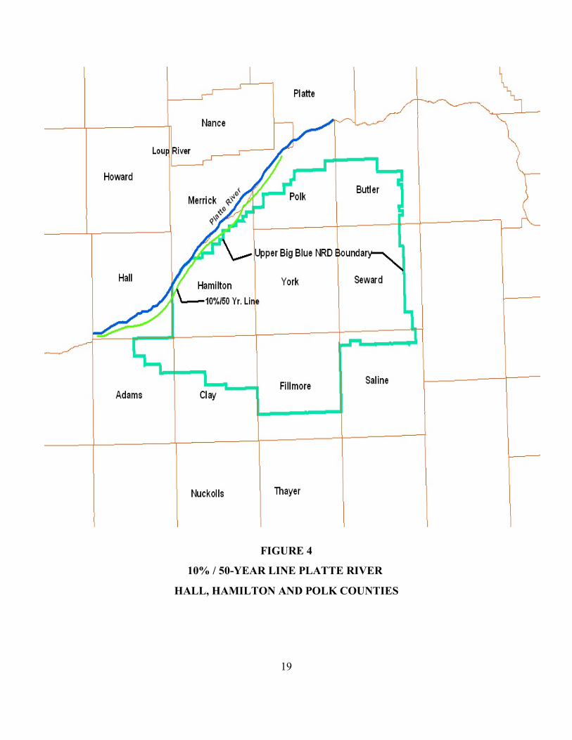
HYDROLOGICALLY CONNECTED AREA

The portion of the Upper Big Blue Natural Resources District that is considered to be

“hydrologically connected” to the Platte River, is that area contained between the Platte River,

the Upper Big Blue NRD boundary, and the 10% / 50 year line. Groundwater pumping wells

contained within this area are determined by the model to have the potential for inducing

additional flow from the Platte River to the underlying aquifer by an amount of at least 10

percent of the volume pumped over a 50-year period. The increase in flow from the river to the

aquifer is presented in terms of the “global” model volumetric budget; i.e., the water pumped

from the well causes an increase in the mass of water moving from the river to the aquifer, but

does not address the transport issues, such as source path or age of water pumped.

A baseline model run, without a pumping well, establishes the volume of water moving

from the river to the aquifer due to non-pumping gradients. Independent model runs are then

made for each new location of the single pumping well. The well is placed at the center of a grid

16

FIGURE 2

PRE-DEVELOPMENT G.W. LEVELS

STARTING HEADS

17

FIGURE 3

FIFTY YEAR MODEL G.W. LEVELS

CHANGES AT OBSERVATION WELLS

Coordinate system is North American Datum, 1983, Nebraska State Plane, Feet.17

18

cell, and the well screen is assumed to be in Layer 2 for each run. The global volumetric budgets

at the end of the 50 stress period are compared with and without pumping, and the difference inth

river flow into the model is used to determine the volume of water induced from the river to the

aquifer due to pumping.

10% / 50-Year Boundary Determination

The 10% / 50-year boundary is determined by evaluating groundwater pumping along

transects, spaced approximately 1 mile apart and perpendicular to the Platte River. Transect cells

that lie on either side of the boundary line are interpolated linearly to determine the actual

coordinates of the boundary line on each transect. Table 3 is a summary of coordinates used to17

establish the 10 / 50 boundary line within the Upper Big Blue NRD. Figures 4 and 5 are

graphical representations of the 10% / 50-year boundary line location.

TABLE 3

10% / 50-YEAR BOUNDARY WITHIN THE UPPER BIG BLUE NRD

STATE PLANE COORDINATES

Easting Northing

2115914.5307 368243.7495

2119524.3678 373861.1446

2122067.5150 377912.3125

2124670.4467 383220.1545

2128158.4452 387639.9242

2132229.2680 391476.8695

2135624.8026 395989.1030

2139012.1417 400512.5376

2140957.5416 402519.5190

2145105.3989 406279.4298

2149493.4078 411118.6532

2153212.8089 415307.0203

19

FIGURE 4

10% / 50-YEAR LINE PLATTE RIVER

HALL, HAMILTON AND POLK COUNTIES

20

FIGURE 5

10% / 50-YEAR LINE PLATTE RIVER

WITHIN THE UPPER BIG BLUE NRD BOUNDARY

APPENDIX A

MODEL BOUNDARY

FIXED FLOW CALCULATIONS

Gradient Gradient Gradient Weighted Weighted 1950 Bottom SaturatedCrossing Angle Perpendicular Hyd. Cond. G.W. Velocity Groundwater Layer 5 Thickness At Boundary Boundary Boundary

Boundary Boundary At Boundary To Boundary At Boundary At Boundary Elevation Elevation Boundary Arc Length Flow Area FlowArc No. (ft./ft.) (deg) (ft./ft.) (ft./d) (ft./d) (ft.>msl) (ft.>msl) (ft.) (ft.) (ft.2) (ft.3/d)

80 -0.000869 90 0.000000 44.3 0.000 1880.0 1660.4 219.6 46,017 10,105,333 038 -0.00208 90 0.000000 69.6 0.000 1833.0 1589.0 244.0 28,340 6,914,960 039 -0.00208 0 -0.002080 54.4 -0.113 1805.0 1557.6 247.4 27,847 6,889,348 -779,54382 -0.00129 90 0.000000 59.8 0.000 1775.0 1551.3 223.7 41,096 9,193,175 023 -0.00089 90 0.000000 109.5 0.000 1740.0 1587.2 152.8 16,903 2,582,778 040 -0.000968 90 0.000000 84.0 0.000 1728.0 1600.4 127.6 30,987 3,953,941 041 -0.002924 72 -0.000904 144.8 -0.131 1680.0 1575.0 105.0 24,486 2,571,030 -336,3841 -0.002000 35 -0.001638 192.1 -0.315 1650.0 1566.5 83.5 24,920 2,080,820 -654,872

42 0.001481 24 0.001353 93.3 0.126 1660.0 1562.9 97.1 35,838 3,479,870 439,26843 0.002000 33 0.001677 82.0 0.138 1632.0 1467.0 165.0 35,201 5,808,165 798,86636 0.002105 67 0.000822 94.2 0.077 1600.0 1410.6 189.4 31,263 5,921,212 458,766

-73,898Total Estimated 1950 Boundary Flow =

Ground Water ModelFixed Flow Boundary Estimates

Southern Boundary1950 G.W. Level - Layer 5

Updated 07/18/05

Gradient Gradient Gradient Weighted Weighted 1950 Bottom SaturatedCrossing Angle Perpendicular Hyd. Cond. G.W. Velocity Groundwater Layer 5 Thickness At Boundary Boundary Boundary

Boundary Boundary At Boundary To Boundary At Boundary At Boundary Elevation Elevation Boundary Arc Length Flow Area FlowArc No. (ft./ft.) (deg) (ft./ft.) (ft./d) (ft./d) (ft.>msl) (ft.>msl) (ft.) (ft.) (ft.2) (ft.3/d)

79 -0.002609 54 -0.001534 34.9 -0.054 1910.0 1698.3 211.7 64,788 13,715,620 -734,06366 -0.001696 49 -0.001113 178.6 -0.199 1735.0 1687.3 47.7 30,975 1,477,508 -293,61667 -0.001885 70 -0.000645 54.3 -0.035 1790.0 1635.3 154.7 46,543 7,200,202 -252,06278 -0.002924 0 0.000000 36.2 0.000 1775.0 1608.3 166.7 9,834 1,639,328 049 -0.002924 0 0.000000 19.3 0.000 1765.0 1611.0 154.0 10,939 1,684,606 050 -0.002924 26 -0.002628 11.1 -0.029 1750.0 1605.0 145.0 18,572 2,692,940 -78,55775 -0.002924 26 -0.002628 18.7 -0.049 1730.0 1598.7 131.3 14,537 1,908,708 -93,80368 -0.002924 26 -0.002628 35.5 -0.093 1715.0 1593.3 121.7 37,939 4,617,176 -430,76769 -0.002827 29 -0.002473 69.4 -0.172 1670.0 1596.3 73.7 33,140 2,442,418 -419,10770 -0.002827 29 -0.002473 121.3 -0.300 1630.0 1544.3 85.7 37,584 3,220,949 -966,02871 -0.002827 29 -0.002473 175.5 -0.434 1595.0 1505.0 90.0 36,660 3,299,400 -1,431,71777 -0.002310 63 -0.001049 121.7 -0.128 1585.0 1468.7 116.3 51,693 6,011,896 -767,29272 -0.002310 63 -0.001049 53.8 -0.056 1505.0 1430.3 74.7 40,925 3,057,098 -172,48537 -0.002310 63 -0.001049 17.7 -0.019 1480.0 1417.5 62.5 3,374 210,875 -3,91474 -0.001571 51 -0.000989 21.5 -0.021 1475.0 1409.0 66.0 31,526 2,080,716 -44,22873 -0.001571 51 -0.000989 18.9 -0.019 1445.0 1365.7 79.3 27,643 2,192,090 -40,961

-5,728,601Total Estimated 1950 Boundary Flow =

Ground Water ModelFixed Flow Boundary Estimates

Northern Boundary1950 G.W. Level - Layer 5

Updated 07/18/05

Gradient Gradient Gradient Weighted Weighted 1950 Bottom SaturatedCrossing Angle Perpendicular Hyd. Cond. G.W. Velocity Groundwater Layer 5 Thickness At Boundary Boundary Boundary

Boundary Boundary At Boundary To Boundary At Boundary At Boundary Elevation Elevation Boundary Arc Length Flow Area FlowArc No. (ft./ft.) (deg) (ft./ft.) (ft./d) (ft./d) (ft.>msl) (ft.>msl) (ft.) (ft.) (ft.2) (ft.3/d)

27 -0.001333 34 -0.001105 13.3 -0.015 1440.0 1323.2 116.8 11,533 1,347,054 -19,7991 -0.001097 59 -0.000565 23.8 -0.013 1443.0 1318.4 124.6 9,800 1,220,753 -16,4155 -0.001296 81 -0.000203 22.8 -0.005 1455.0 1304.0 151.0 15,820 2,388,820 -11,0422 -0.001296 81 -0.000203 14.0 -0.003 1480.0 1298.4 181.6 23,550 4,276,680 -12,1393 -0.002455 41 -0.001853 12.8 -0.024 1487.0 1302.1 184.9 26,940 4,981,206 -118,1344 0.002261 0 0.000000 20.7 0.000 1555.0 1260.0 295.0 51,610 15,224,950 06 -0.002665 75 -0.000690 21.4 -0.015 1570.0 1207.1 362.9 33,086 12,006,909 -177,230

19 -0.001964 50 -0.001262 31.6 -0.040 1505.0 1206.0 299.0 26,280 7,857,720 -313,46818 -0.001399 29 -0.001224 35.8 -0.044 1485.0 1210.9 274.1 34,070 9,338,587 -409,07317 -0.001399 29 -0.001224 52.3 -0.064 1473.0 1191.8 281.2 8,860 2,491,432 -159,43625 -0.001399 29 -0.001224 32.8 -0.040 1465.0 1267.9 197.1 24,300 4,789,530 -192,22216 -0.001565 74 -0.000431 24.3 -0.010 1472.0 1318.6 153.4 18,560 2,847,104 -29,84415 -0.001565 74 -0.000431 62.0 -0.027 1500.0 1318.3 181.7 19,950 3,624,915 -96,94914 -0.001565 74 -0.000431 124.9 -0.054 1520.0 1310.1 209.9 13,430 2,818,957 -151,88113 -0.001565 74 -0.000431 131.8 -0.057 1540.0 1308.8 231.2 12,850 2,970,920 -168,91112 -0.001565 74 -0.000431 138.2 -0.060 1552.0 1328.8 223.2 10,080 2,249,856 -134,12711 -0.001565 74 -0.000431 100.4 -0.043 1570.0 1371.8 198.2 13,820 2,739,124 -118,63110 -0.001565 74 -0.000431 52.5 -0.023 1590.0 1409.6 180.4 8,470 1,527,988 -34,6049 -0.001565 90 0.000000 45.2 0.000 1600.0 1425.0 175.0 5,450 953,750 08 -0.001565 90 0.000000 35.1 0.000 1615.0 1449.2 165.8 12,070 2,001,206 07 -0.001565 90 0.000000 22.4 0.000 1630.0 1489.1 140.9 9,460 1,332,914 0

26 -0.001399 90 -0.001399 23.4 -0.033 1638.0 1512.3 125.7 18,456 2,319,919 -75,94620 -0.001399 90 -0.001399 72.3 -0.101 1640.0 1471.9 168.1 28,943 4,865,318 -492,11621 -0.001399 90 -0.001399 30.0 -0.042 1647.0 1506.0 141 30,370 4,282,170 -179,72322 -0.001794 41 -0.001354 77.2 -0.105 1595.0 1388.6 206.4 52,830 10,904,112 -1,139,75123 -0.001696 22 -0.001573 117.6 -0.185 1577.0 1314.5 262.5 14,429 3,787,613 -700,43024 -0.001555 7 -0.001543 109.1 -0.168 1575.0 1364.0 211 35,841 7,562,451 -1,273,411

-6,025,283Total Estimated 1950 Boundary Flow =

Ground Water ModelFixed Flow Boundary Estimates

Eastern Boundary1950 G.W. Level - Layer 5

Updated 07/18/05

Gradient Gradient Gradient Weighted Weighted 1950 Bottom SaturatedCrossing Angle Perpendicular Hyd. Cond. G.W. Velocity Groundwater Layer 5 Thickness At Boundary Boundary Boundary

Boundary Boundary At Boundary To Boundary At Boundary At Boundary Elevation Elevation Boundary Arc Length Flow Area FlowArc No. (ft./ft.) (deg) (ft./ft.) (ft./d) (ft./d) (ft.>msl) (ft.>msl) (ft.) (ft.) (ft.2) (ft.3/d)

1 0.000891 0 0.000891 29.5 0.026 1902.0 1745.3 156.7 10,227 1,602,571 42,1232 0.001382 45 0.000977 56.5 0.055 1903.0 1782.5 120.5 12,141 1,462,991 80,7764 0.003388 26.5 0.003032 50.5 0.153 1920.0 1812.4 107.6 9,090 978,084 149,76212 0.002875 18.4 0.002728 45.0 0.123 1932.0 1811.7 120.3 12,930 1,555,479 190,9523 0.002964 26.5 0.002653 48.5 0.129 1930.0 1784.8 145.2 13,060 1,896,312 243,96113 0.002341 34.5 0.001929 54.1 0.104 1955.0 1720.3 234.7 26,130 6,132,711 640,0965 0.002145 19.3 0.002024 51.6 0.104 1985.0 1694.7 290.3 25,910 7,521,673 785,7276 0.001969 17.6 0.001877 50.0 0.094 2008.0 1768.2 239.8 40,530 9,719,094 912,0567 0.001607 45 0.001136 40.7 0.046 2003.0 1818.3 184.7 35,491 6,555,188 303,16614 0.001786 45 0.001263 31.9 0.040 1982.0 1797.9 184.1 11,750 2,163,175 87,1468 0.001684 0 0.001684 17.6 0.030 1972.0 1759.4 212.6 34,700 7,377,220 218,6499 0.001684 0 0.001684 10.0 0.017 1978.0 1731.2 246.8 14,990 3,699,532 62,30010 0.001752 27.6 0.001553 9.2 0.014 1978.0 1722.8 255.2 10,340 2,638,768 37,69311 0.001906 56.9 0.001041 19.2 0.020 1960.0 1713.6 246.4 19,299 4,755,274 95,033

3,849,440Total Estimated 1950 Boundary Flow =

Ground Water ModelFixed Flow Boundary Estimates

Western Boundary1950 G.W. Level - Layer 5

Updated 07/18/05

APPENDIX B

RIVER BED CONDUCTANCE

PLATTE RIVER

Transect Site Kv1 Kv2 Ecbase M1 M2 Kv L W M C(ft/d) (ft/d) (mS/m) (ft) (ft) (ft/d) (ft) (ft) (ft) (ft2/d/ft)

A1 NC 78.7 0.056 35 13.8 6.8 0.169 1 1 20.6 0.0082A2 MC 78.7 0.056 35 15.9 6.9 0.185 1 1 22.8 0.0081A3 SC 78.7 0.056 35 12.4 13.3 0.108 1 1 25.7 0.0042B1 NC 109.7 0.056 35 21.6 1.7 0.763 1 1 23.3 0.0327B2 MC 109.7 0.056 35 10.8 9.5 0.120 1 1 20.3 0.0059B3 SC 109.7 0.056 35 8.5 8.1 0.115 1 1 16.6 0.0069

Average Unit C = 0.0110 ft2/d per foot of river reach per foot of river widthTotal Conductance C 11.0 ft2/d per foot of river reach (using a river bed with of 1,000 ft.)

NOTES:1. NC = North Channel2. MC = Middle Channel3. SC = South Channel4. Site A is located in Sec 29, Twp 11N, Rng 8W, and is upstream from the BNSF railroad bridge over the Platte River near Grand Island5. Site B is located in the NW4 Sec 11, Twp 11N, Rng 8W, and is near the upstream from the Chapman Bridge near the intersection of 5th and B Streets 6. Kv1 = vertical hydraulic conductivity of river bed material with EC log < 35 mS/m7. Kv2 = vertical hydraulic conductivity of river bed material with EC log >= 35 mS/m8. Kv = wighted vertical hydraulic conductivity for total river bed thickness M9. L = river reach length (use 1.0 ft. for this calculation)10. W = river bed width (use 1.0 ft. to compute the unit condutance. Apply total river bed width of 1,000 ft. to determine total bed conductance per linear foot of river reach between Hwy. 34 bridge and Chapman bridge11. M1 = thickness of the river bed material with EC log < 35 mS/m) (based on CSD geoprobe resistivity log)12. M2 = thickness of the river bed material with EC log >= 35 mS/m) (based on CSD geoprobe resistivity log)13. M = total river bed thickness (M1 + M2)14. Equation for computing river bed conductance Kv x L x W C = ------------------------ M

15. Equation for weighting vertical hydraulic conductivity: M Kv = ---------------------------------- (M1/Kv1) + (M2/Kv2)

Platte RiverAverage Bed Conductance

Between Hwy. 34 And Chapman BridgesBased On Permeameter Tests and Geoprobe Borings

UNL Conservation and Survey - August 2005

APPENDIX CGROUNDWATER LEVEL MAPS

DEPTH TO GROUNDWATER

23

FIGURE 7

GENERAL GROUNDWATER ELEVATION MODEL

24

FIGURE 8

GENERAL DEPTH OF GROUNDWATER BELOW LAND SURFACE