Groundwater Flow Systems in Mountainous Terrain 1

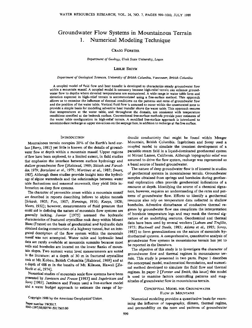
WATER RESOURCES RESEARCH, VOL. 24, NO. 7, PAGES 999-1010, JULY I988

Groundwater Flow Systems in Mountainous Terrain 1. Numerical Modeling Technique

CRAIG FORSTER

Department of Geology, Utah State University, Logan

LESLIE SMITH

Department of Geological Sciences, University of British Columbia, Vancouver, British Columbia

A coupled model of fluid flow and heat transfer is developed to characterize steady groundwater flow within a mountain massif. A coupled model is necessary because high-relief terrain can enhance groundwater flow to depths where elevated temperatures are encountered. A wide range in water table form and elevation expected in high-relief terrain is accommodated using a free-surface method. This approach allows us to examine the influence of thermal conditions on the patterns and rates of groundwater flow and the position of the water table. Vertical fluid flow is assumed to occur within the unsaturated zone to provide a simple basis for modeling advective heat transfer above the water table. This approach ensures that temperatures at the water table, and throughout the domain, are consistent with temperature conditions sl•ecified at the bedrock surface. Conventional free-surface methods provide poor estimates of the water table configuration in high-relief terrain. A modified free-surface approach is introduced to accommodate recharge at upper elevations on the seepage face, in addition to recharge at the free surface.

INTRODUCTION

Mountainous terrain occupies 20% of the Earth's land surface [Barry, 1981] yet little is known of the details of groundwater flow at depth within a mountain massif. Upper regions of flow have been explored, to a limited extent, in field studies that emphasize the interface between surface hydrology and shallow groundwater flow [Halstead, 1969; Sklash and Farvol- den, 1979; Bortolami et al., 1979; Martinec et al., 1982; Smart, 1985]. Although these studies provide insight into the hydrology of alpine watersheds and the relationships between water table fluctuations and seasonal snowmelt, they yield little information on deep flow systems.

The character of permeable zones within a mountain massif are described in reports describing inflows to alpine tunnels [$chardt, 1905; Fox, 1907; Hennings, 1910; Keays, 1928; Meats, 1932]; however, measurements of fluid pressure that could aid in defining the nature of mountain flow systems are generally lacking. Jamier [1975] assessed the hydraulic characteristics of fractured crystalline rock deep within Mount Blanc (France) on the basis of geochemical and hydraulic data obtained during construction of a highway tunnel, but an inte- grated description of the flow system within the mountain massif was not attempted. Water table and hydraulic head data are rarely available at mountain summits because most wells and boreholes are located on the lower flanks of mountain slopes. Two summit water level measurements are noted in the literature- at a depth of 30 m in fractured crystalline rock at Mt. Kobau, British Columbia [Halstead, 1969] and at a depth of 488 m in the basalts of Mt. Kilauea, Hawaii [Za- blocki et al., 1974].

Numerical studies of mountain scale flow systems have been presented by Jamieson and Freeze [1983] and lngebritsen and Sorey [1985]. Jamieson and Freeze used a free-surface model and a water budget approach to estimate the range of hy-

Copyright 1988 by the American Geophysical Union. Paper number 7W5017. 0043-1397/88/007W_5017505.00

draulic conductivity that might be found within Meager Mountain, British Columbia. Ingebritsen and Sorey used a coupled model to simulate the transient development of a parasitic steam field in a liquid-dominated geothermal system at Mount Lassen, California. Although topographic relief was assumed to drive the flow system, recharge was represented as a basal source of heated groundwater.

The nature of deep groundwater flow is of interest in studies of geothermal systems in mountainous terrain. Groundwater samples obtained from springs and boreholes during geothermal exploration often provide geochemical indications of a resource at depth. Identifying the source of a chemical signa- ture, however, requires an understanding of the rates and patterns of groundwater flow. Efforts to identify a geothermal resource also rely on temperature data collected in shallow boreholes. Advective disturbance of conductive thermal re-

gimes by groundwater flow can complicate the interpretation of borehole temperature logs and may mask the thermal sig- nature of an underlying resource. Geochemical and thermal data have been used by several workers [Lahsen and Trujillo, 1975; Blackwell and Steele, 1983; Adams et al., 1985; Sorey, 1985] to form generalizations on the nature of mountain hydrothermal systems. A comprehensive, quantitative analysis of groundwater flow systems in mountainous terrain has yet to be reported in the literature.

The objective of this study is to investigate the character of groundwater flow and thermal regimes in mountainous terrain. This study is presented in two parts. Paper 1 describes the conceptual model, mathematical formulation, and numerical method developed to simulate the fluid flow and thermal regimes. In paper 2 [Forster and Smith, this issue] this model is used to examine factors controlling patterns and mag- nitudes of groundwater flow in mountainous terrain.

CONCEPTUAL MODEL FOR GROUNDWATER

FLOW IN MOUNTAINS

Numerical modeling provides a quantitative basis for examining the influence of topography, climate, thermal regime, and permeability on the rates and patterns of groundwater

999

1000 FORSTER AND SMITH: GROUNDWATER ];'LOW SYSTEMS,

(a)

o

-1

-2

0 4 8 12 16 2o

z (b) • 2 < 1

0 4 8 12 16 20

(c) 0.$

o 4 8 16 20

DISTANCE (km)

Water table • Hypothetical groundwater pathline

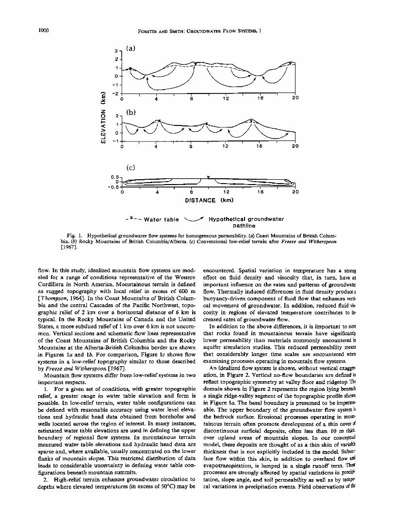
Fig. 1. Hypothetical groundwater flow systems for homogeneous permeability. (a) Coast Mountains of British Colum- bia. (b) Rocky Mountains of British Columbia/Alberta. (c) Conventional low-relief terrain after Freeze and Witherspoon [1967].

flow. In this study, idealized mountain flow systems are modeled for a range of conditions representative of the Western Cordillera in North America. Mountainous terrain is defined

as rugged topography with local relief in excess of 600 m [Thompson, 1964]. In the Coast Mountains of British Colum- bia and the central Cascades of the Pacific Northwest, topographic relief of 2 km over a horizontal distance of 6 km is typical. In the Rocky Mountains of Canada and the United States, a more subdued relief of 1 km over 6 km is not uncom- mon. Vertical sections and schematic flow lines representative of the Coast Mountains of British Columbia and the Rocky Mountains at the Alberta-British Columbia border are shown

in Figures la and lb. For comparison, Figure lc shows flow systems in a low-relief topography similar to those described by Freeze and Witherspoon [1967].

Mountain flow systems differ from low-relief systems in two important respects.

1. For a given set of conditions, with greater topographic relief, a greater range in water table elevation and form is possible. In low-relief terrain, water table configurations can be defined with reasonable accuracy using water level elevations and hydraulic head data obtained from boreholes and wells located across the region of interest. In many instances, estimated water table elevations are used in defining the upper boundary of regional flow systems. In mountainous terrain measured water table elevations and hydraulic head data are sparse and, where available, usually concentrated on the lower flanks of mountain slopes. This restricted distribution of data leads to considerable uncertainty in defining water table configurations beneath mountain summits.

2. High-relief terrain enhances groundwater circulation to depths where elevated temperatures (in excess of 50øC) may be

encountered. Spatial variation in temperature has a strong effect on fluid density and viscosity that, in turn, have an important influence on the rates and patterns of groundwater flow. Thermally induced differences in fluid density produce a buoyancy-driven component of fluid flow that enhances vertical movement of groundwater. In addition, reduced fluid viscosity in regions of elevated temperature contributes to increased rates of groundwater flow.

In addition to the above differences, it is important to note that rocks found in mountainous terrain have significantl)' lower permeability than materials commonly encountered in aquifer simulation studies. This reduced permeability means that considerably longer time scales are encountered when examining processes operating in mountain flow systems.

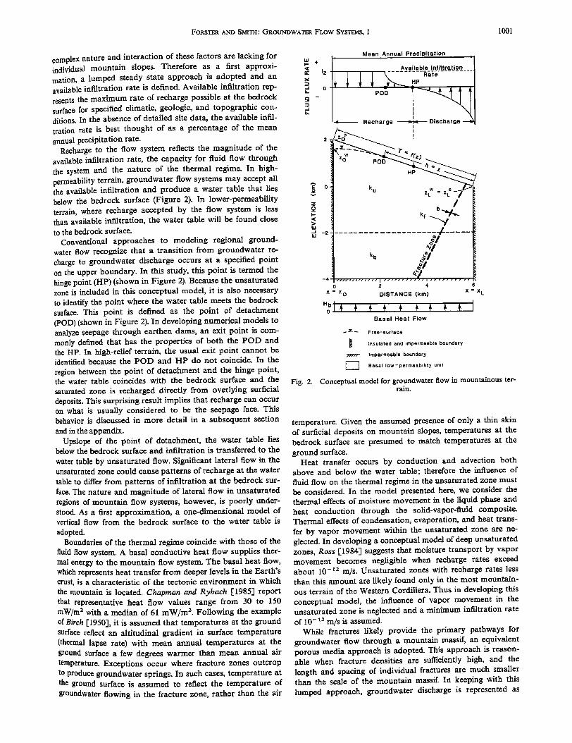
An idealized flow system is shown, without vertical exagger- ation, in Figure 2. Vertical no-flow boundaries are defined to reflect topographic symmetry at valley floor and ridgetop. The domain shown in Figure 2 represents the region lying beneath a single ridge-valley segment of the topographic profile shown in Figure la. The basal boundary is presumed to be impermeable. The upper boundary of the groundwater flow system is the bedrock surface. Erosional processes operating in mountainous terrain often promote development of a thin cover of discontinuous surficial deposits, often less than 10 m thick. over upland areas of mountain slopes. In our concept• model, these deposits are thought of as a thin skin of variable thickness that is not explicitly included in the model. Subsur. face flow within this skin, in addition to overland flow and evapotranspiration, is lumped in a single runoff term. These processes are strongly affected by spatial variations in precipi' tation, slope angle, and soil permeability as well as by tempo' ral variations in precipitation events. Field observations of the

Foast•a Arqn SM•T•' GROUNDWATER Frow S¾s•:œMs, 1 10131

complex nature and interaction of these factors are lacking for individual mountain slopes. Therefore as a first approximation, a lumped steady state approach is adopted and an available infiltration rate is defined. Available infiltration represents the maximum rate of recharge possible at the bedrock surface for specified climatic, geologic, and topographic conditions. In the absence of detailed site data, the available infiltration rate is best thought of as a percentage of the mean annual precipitation rate.

Recharge to the flow system reflects the magnitude of the available infiltration rate, the capacity for fluid flow through the system and the nature of the thermal regime. In high- permeability terrain, groundwater flow systems may accept all the available infiltration and produce a water table that lies below the bedrock surface (Figure 2). In lower-permeability terrain, where recharge accepted by the flow system is less than available infiltration, the water table will be found close to the bedrock surface.

Conventional approaches to modeling regional groundwater flow recognize that a transition from groundwater recharge to groundwater discharge occurs at a specified point on the upper boundary. In this study, this point is termed the hinge point (HP) (shown in Figure 2). Because the unsaturated zone is included in this conceptual model, it is also necessary to identify the point where the water table meets the bedrock surface. This point is defined as the point of detachment (POD) (shown in Figure 2). In developing numerical models to analyze seepage through earthen dams, an exit point is commonly defined that has the properties of both the POD and the HP. In high-relief terrain, the usual exit point cannot be identified because the POD and HP do not coincide. In the region between the point of detachment and the hinge point, the water table coincides with the bedrock surface and the saturated zone is recharged directly from overlying surficial deposits. This surprising result implies that recharge can occur on what is usually considered to be the seepage face. This behavior is discussed in more detail in a subsequent section and in the appendix.

Upslope of the point of detachment, the water table lies below the bedrock surface and infiltration is transferred to the water table by unsaturated flow. Significant lateral flow in the unsaturated zone could cause patterns of recharge at the water table to differ from patterns of infiltration at the bedrock surface. The nature and magnitude of lateral flow in unsaturated regions of mountain flow systems, however, is poorly under- stood. As a first approximation, a one-dimensional model of vertical flow from the bedrock surface to the water table is adopted.

Boundaries of the thermal regime coincide with those of the fluid flow system. A basal conductive heat flow supplies thermal energy to the mountain flow system. The basal heat flow, which represents heat transfer from deeper levels in the Earth's crust, is a characteristic of the tectonic environment in which the mountain is located. Chapman and Rybach [1985] report that representative heat flow values range from 30 to 150 mW/m 2 with a median of 61 mW/m 2. Following the example of Birch [1950], it is assumed that temperatures at the ground surface reflect an altitudinal gradient in surface temperature {thermal lapse rate) with mean annual temperatures at the ground surface a few degrees warmer than mean annual air temperature. Exceptions occur where fracture zones outcrop to produce groundwater springs. In such cases, temperature at the ground surface is assumed to reflect the temperature of groundwater flowing in the fracture zone, rather than the air

Mean Annual Precipitation

Available Infiltration <• •z -•'a• .........

• ø I - PO

C3 -

,, i

Recharge I

)

v • 1.•

z o b

• kf ........

0 2 4 6

x = x O DISTANCE (km) x = x L

Basal Heat Flow

• _v. • Free-surface

• Insulated an• •mpermeable boundary • Impermeable boundary

:"•:• Basal low-permeability unit

Fig. 2. Conceptual model for groundwater flow in mountainous terrain.

temperature. Given the assumed presence of only a thin skin of surficial deposits on mountain slopes, temperatures at the bedrock surface are presumed to match temperatures at the ground surface.

Heat transfer occurs by conduction and advection both above and below the water table; therefore the influence of fluid flow on the thermal regime in the unsaturated zone must be considered. In the model presented here, we consider the thermal effects of moisture movement in the liquid phase and heat conduction through the solid-vapor-fluid composite. Thermal effects of condensation, evaporation, and heat transfer by vapor movement within the unsaturated zone are neglected. In developing a conceptual model of deep unsaturated zones, Ross [1984] suggests that moisture transport by vapor movement becomes negligible when recharge rates exceed about 10-•2 m/s. Unsaturated zones with recharge rates less than this amount are likely found only in the most mountainous terrain of the Western Cordillera. Thus in developing this conceptual model, the influence of vapor movement in the unsaturated zone is neglected and a minimum infiltration rate of 10-t2 m/s is assumed.

While fractures likely provide the primary pathways for groundwater flow through a mountain massif, an equivalent porous media approach is adopted. This approach is reasonable when fracture densities are sufficiently high, and the length and spacing of individual fractures are much smaller than the scale of the mountain massif. In keeping with this lumped approach, groundwater discharge is represented as

1002 FORSTSR ^ND SMITH: GrtOUNDWATSR FLOW S¾STSMS, 1

seepage distributed across the discharge area (downslope of the HP in Figure 2), rather than at isolated groundwater springs. Local variations in surface topography, rock permeability, and thickness of surficial deposits controlling the distribution of springs are assumed to have little effect on the overall pattern and magnitude of groundwater flow. Excep- tions to this assumption are caused by major throughgoing fracture zones represented as discrete permeable fracture zones with a homogeneous permeability k s and width b (Figure 2).

MATHEMATICAL MODEL

The mathematical model for groundwater flow in mountains is expressed by two coupled partial differential equations describing fluid flow and heat transfer, by equations of state for the temperature and pressure dependance of fluid density and viscosity, and by boundary conditions for both the fluid and thermal problems. The steady state equation of fluid mass conservation in the absence of internal sources and sinks is

given by

c9-• Ep sq•] + •zz Ep fq•] = 0 (1)

where Pt = pœ(T, p) is fluid density and q,• and q= are horizontal and vertical components of fluid flux (specific discharge), respectively. Fluid flow is driven by gradients in fluid pressure and thermally induced density contrasts. Fluid potential h is defined in terms of an equivalent freshwater head:

(2)

where P0 is a reference fluid density at a specified temperature, g is acceleration due to gravity, p is fluid pressure, and z is the elevation where the freshwater head is calculated. Frind

[1982] advocates the use of an equivalent freshwater head to describe potential gradients exclusive of static fluid pressures.

Fluid flux through the saturated porous matrix is given by

q' = --V Pog O•j + (p•' -- Po)g (3) where p = p(T, p) is the dynamic viscosity of the fluid and k U is the permeability tensor for the porous matrix. This equation is simplified by defining a relative density

to obtain

q•= --k u• +p, (5) In thin fracture zones and discrete fractures, fluid flux in

direction s parallel to the fracture-matrix boundary is given by

poq [c3h •z] qs: --kz • •ss + p" •ss (6) where kz is the permeability of material within a discrete fracture or fracture zone. For open fractures, a parallel plate model is used to define the fracture permeability in terms of an effective aperture b where kz = b2/12.

The equation describing the distribution of freshwater head in the porous matrix is obtained by substituting (5) into (1):

=o (7)

The cross terms for the permeability tensor (k,=, k=x ) are in. cluded to preserve the generality of the subsequent numerical formulation. The analagous equation in one-dimensional local coordinates for a fracture zone is

7; :0 Boundary conditions for the fluid flow system shown in

Figure 2 are as follows:

Oh for --4km<z<_z• • - 0 (9a)

tax at x = x o x = x L

Oh for x 0 < x < x•. --= o (%1 c3z at z = --4 km

for x o < x <_ x•. h = zx" (9c}

at z = Zx w

where x o equals 0.0 km, L is the horizontal length of the fl0w system (6.0 km), and z,• • is the water table elevation at the specified x coordinate.

In Figure 2, the free surface is that portion of the water table that lies below the bedrock surface. Equation (9c) reflects the fact that freshwater head must equal the water table eleva. tion everywhere at the upper boundary of the saturated region of flow. On the free-surface segment an additional constraint is required to limit the infiltration available for recharge to the bedrock flow system. Fluid flux q•,, directed along the unit normal n• to the free surface, is driven by potential gradients and thermal buoyancy where

= - -- n• = (I_. cos O)n• q• ku • + P• (10)

The available infiltration rate I= is applied directly on the free surface to represent one-dimensional flow from the bedrock surface to a water table that slopes at an angle 0 from horizontal. This boundary condition differs from that used bs, Neuman and Witherspoon [1970] in two respects. First, fluid flux and freshwater head conditions are specified on the free- surface segment while only freshwater head is specified on the seepage face (Figure 2). This approach allows recharge to occur on the seepage face between HP and POD. Below the HP, only discharge occurs. Second, a buoyancy term stated in terms of the relative buoyancy p• is included inside the square brackets of (I 0) because thermal effects are incorporated in the formulation. The appendix contains a discussion of the conditions that promote separation of the POD and HP and outlines use of a hodograph to demonstrate the theoretical basis for such a separation.

The steady state balance of thermal energy in a variab!y saturated porous medium with no internal heat sources or sinks is described by

c3 [/1.xx * cST c3T] c•[ 8T OT --Piti q,•xx + q='•z'z =0 (11)

where

T temperature;

FORSTER AND SMITH: GROUNDWATER FLOW SYSTEMS, 1 1003

Cs specific heat capacity of fluid; 2•f thermal conductivity tensor for solid-fluid-vapor

composite.

The last term on the left side of (11) describes the advective transfer of heat by fluid flow both above and below the water table. In (11), thermal equilibrium is assumed to exist between fluid, solid, and vapor.

Modeling heat transfer in the unsaturated zone ensures a water table temperature and thermal regime consistent with temperature conditions specified at the bedrock surface. By adopting a free-surface method, the rate of vertical fluid flow in the unsaturated zone is defined to be the available infiltration rate (applied directly on the free surface). In solving the equations of energy transport, one-dimensional advective heat transfer above the water table is modeled by setting the horizontal fluid flux q•, to zero and the vertical fluid flux q.. to the available infiltration rate I.. in (11).

Heat conduction and thermal dispersion by fluid flow in the solid-liquid-vapor composite is represented by the first two terms of (11) using a thermal conductivity tensor defined by

,•if -- SnDi• + (1 -- S)n2 •' + (1 -- n)J,u s (12)

where

n porosity of the porous matrix; )?' thermal conductivity of vapor;

Dij conduction-dispersion tensor for fluid; ).tj s thermal conductivity tensor for solid;

S degree of saturation (S -- 1 below water table; 0 < S _< 1 above water table).

In this formulation, the degree of saturation above the water table is specified only to calculate the thermal conductivity of the solid-fluid-vapor composite found above the water table. The degree of saturation reflects the relative proportion of vapor and fluid within the pore space and may vary from less than 0.2 to 1.0 within the unsaturated zone. Because the thero

real conductivity of air is about 5% that of water, higher levels of saturation S contribute to greater thermal conductivity. Rocks most commonly found in mountainous terrain are likely to have porosity values less than about 15%. Therefore the degree of saturation has little impact on values calculated for thermal conductivity of the solid-vapor-fluid composite. In the absence of information regarding the variability of saturation in mountainous terrain, the pore space is assumed to be filled only with vapor (S -- 0). Although a minimum degree of saturation is required to permit fluid flow in the unsaturated zone, this assumption provides an upper limit for the influence of saturation on mountain flow systems by contributing to a minimum estimate of thermal conductivity above the water table. Note that the thermal conductivity for a composite porous media is defined using the arithmetic mean to account for the thermal conductivity of each material. This approach is commonly adopted in the hydrogeology literature [Sorey, 1978; Smith and Chapman, 1983]. This approach differs from that found in the heat flow literature, a fact that reflects different views regarding the influence of porosity on thermal conductivity [Walsh and Decker, 1966; Scharli and Rybach, 1984-1.

Bear [1972] uses a fluid conduction-dispersion tensor D O to account for both heat conduction in the fluid and thermal

dispersion by mechanical mixing. The nature of thermal dispersion in a porous medium is described by Sauty et al. [1982]. Bear [1979] shows that the dispersion terms can be

expanded for an isotropic porous medium as follows:

nDxx = psCs(atqx2/• q- atq:2/tj) q-

nD.... -- pfCf(atqx2/• -b atq:2/cj) + n2 œ

nD,½.. = nD:,, = pœCœ(a t - at)qxq../c 7

(13a)

(13b)

(13c)

Here, a t and a t are longitudinal and transverse dispersivities, 3f is the thermal conductivity of the fluid, and • is the magnitude of the fluid flux.

The analagous energy balance equation for a fully saturated fracture zone is written using one-dimensional local coordinates as

•ss n'cDs + (I -- n f)2 s c•T c?T '•-J's- PsC'rq• • = 0 (14) where

nsDs --' pj. Cj.(atqs + nf,t f) (15)

In (14) and (15), nœ is the porosity of the fracture, where 0 < nœ < 1 for fractures filled with porous material and n s equals 1 for open fractures. Where n s is less than 1, an isotropic thermal conductivity ,U is assumed for the fracture filling.

Boundary conditions for the heat transfer problem are

•T for --4km<z<z• • - 0 (16a)

•X at X

c3T for x o _< x _< ,•..e • = H• (16b) -' at z= -4 km

for x o _< x _< T = T, + G•z.•S (16c)

at z = zx •

where H• is the conductive basal heat flow, T• is a reference surface temperature specified at the valley floor, Gt is a thermal lapse rate applied at the bedrock surface, and, z• s is the surface elevation at the specified x coordinate position. Ther- mal springs are modeled where fracture zones outcrop at the bedrock surface by assuming that the heat flux from the fracture zone is equal to the advective flux of heat along the fracture zone. With only advective flux presumed to occur at the fracture outcrop, a specified temperature is not required and the bedrock temperature is dictated by the temperature of the fluid discharging from the fracture zone (a third-type boundary condition).

The fluid is assumed to be pure liquid water with density and viscosity a function only of temperature and pressure. Water properties are evaluated using the relationships of Keenan et al. 1-1978] for density and of Watson et al. [198171 for viscosity. Specific heat capacity and thermal conductivity of water is assumed constant, as is the thermal conductivity of vapor in the unsaturated zone. Porosity, permeability, and thermal conductivity vary in space but are assumed indepen- dent of temperature and pressure.

NUMERICAL METHOD

The Galerkin finite element method is used to solve the

coupled equations of steady fluid flow and heat transfer. Two- dimensional vertical sections of porous media with planar or radial symmetry are represented by linear triangular elements. Thin, high-permeability fracture zones are included by em- bedding one-dimensional line elements in the field of triangular elements using the method described by Baca et al. [1984].

1004 FORSTER AND SMITH: GROUNDWATER FLOW SYSTEMS, 1

bo

-2

-4

ILl -2

-4

0 2 4 6

0 2 4 6

DISTANCE (km)

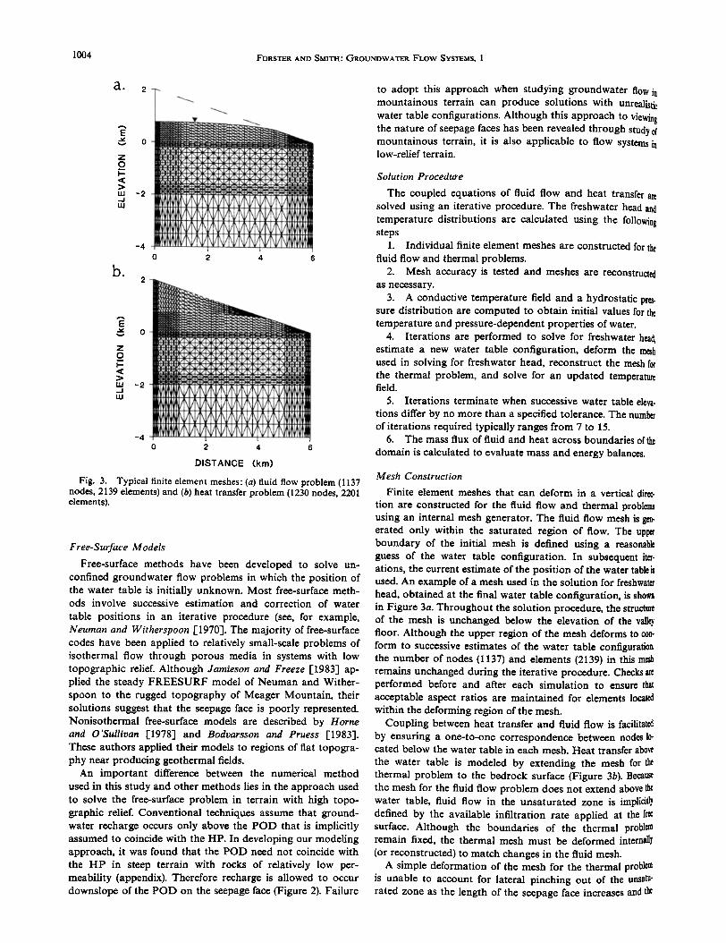
Fig. 3. Typical finite element meshes: (a) fluid flow problem (1137 nodes, 2139 elements) and (b) heat transfer problem (1230 nodes, 2201 elements).

Free-Smfiwe Models

Free-surface methods have been developed to solve un- confined groundwater flow problems in which the position of the water table is initially unknown. Most free-surface methods involve successive estimation and correction of water

table positions in an iterative procedure (see, for example, Neuman and Witherspoon [-1970]. The majority of free-surface codes have been applied to relatively small-scale problems of isothermal flow through porous media in systems with low topographic relief. Although Jamieson and Freeze [1983] applied the steady FREESURF model of Neuman and Wither- spoon to the rugged topography of Meager Mountain, their solutions suggest that the seepage face is poorly represented. Nonisothermal free-surface models are described by Horne and O'Sullivan [1978] and Bodvarsson and Pruess [1983]. These authors applied their models to regions of flat topography near producing geothermal fields.

An important difference between the numerical method used in this study and other methods lies in the approach used to solve the free-surface problem in terrain with high topographic reliefi Conventional techniques assume that groundwater recharge occurs only above the POD that is implicitly assumed to coincide with the HP. In developing our modeling approach, it was found that the POD need not coincide with the HP in steep terrain with rocks of relatively low permeability (appendix). Therefore recharge is allowed to occur downslope of the POD on the seepage face (Figure 2). Failure

to adopt this approach when studying groundwater flow in mountainous terrain can produce solutions with unrealistic water table configurations. Although this approach to viewing the nature of seepage faces has been revealed through study of mountainous terrain, it is also applicable to flow systems in low-relief terrain.

Solution Procedure

The coupled equations of fluid flow and heat transfer are solved using an iterative procedure. The freshwater head and temperature distributions are calculated using the following steps

1. Individual finite element meshes are constructed for the fluid flow and thermal problems.

2. Mesh accuracy is tested and meshes are reconstructed as necessary.

3. A conductive temperature field and a hydrostatic pres. sure distribution are computed to obtain initial values for the temperature and pressure-dependent properties of water.

4. Iterations are performed to solve for freshwater head. estimate a new water table configuration, deform the mesh used in solving for freshwater head, reconstruct the mesh for the thermal problem, and solve for an updated temperature fie!&

5. Iterations terminate when successive water table elena. tions differ by no more than a specified tolerance. The number of iterations required typically ranges from 7 to 15.

6. The mass flux of fluid and heat across boundaries of the

domain is calculated to evaluate mass and energy balances.

l•'lesh Construction

Finite element meshes that can deform in a vertical direc-

tion are constructed for the fluid flow and thermal problems using an internal mesh generator. The fluid flow mesh is generated only within the saturated region of flow. The upper boundary of the initial mesh is defined using a reasonable guess of the water table configuration. In subsequent iterations, the current estimate of the position of the water table is used. An example of a mesh used in the solution for freshwater head, obtained at the final water table configuration, is shown in Figure 3a. Throughout the solution procedure, the structure of the mesh is unchanged below the elevation of the valle.• floor. Although the upper region of the mesh deforms to conform to successive estimates of the water table configuration. the number of nodes (1137) and elements (2139) in this mesl: remains unchanged during the iterative procedure. Checks are performed before and after each simulation to ensure that acceptable aspect ratios are maintained for elements located within the deforming region of the mesh.

Coupling between heat transfer and fluid flow is facilitatea by ensuring a one-to-one correspondence between nodes 10- cated below the water table in each mesh. Heat transfer ab0•e

the water table is modeled by extending the mesh for the thermal problem to the bedrock surface (Figure 3b). Because the mesh for the fluid flow problem does not extend above the water table, fluid flow in the unsaturated zone is implicitl.• defined by the available infiltration rate applied at the free surface. Although the boundaries of the thermal problem remain fixed, the thermal mesh must be deformed internall.• {or reconstructed) to match changes in the fluid mesh.

A simple deformation of the mesh for the thermal problem is unable to account for lateral pinching out of the unsaturated zone as the length of the seepage face increases and the

FORSTER AND SMITH: GROUNDWATER FLOW SYSTEMS, 1 1005

POD moves upslope on the bedrock surface during the iterative procedure. Therefore the thermal mesh must be reconstructed in its entirety at each iteration to accomodate upslope or downslope movement of the POD. Each time the mesh is reconstructed, the number of nodes and elements may change depending upon the degree of POD movement. A final thermal mesh, which corresponds to the fluid mesh of Figure 3a, is shown in Figure 3b and contains 1230 nodes and 2201 elements. The numerical formulation does not include a method for maintaining the position of fracture zones and geologic boundaries within deforming regions of the mesh. As a consequence, fracture zones and heterogeneities must be restricted to nondeforming regions of the mesh.

The accuracy of each initial mesh is evaluated by solving the isothermal fluid flow problem and computing a total balance of fluid mass crossing all system boundaries and a fluid mass balance across the top surface. Because vertical grid lines in the deforming mesh are rarely orthogonal to the sloping top boundary, computing fluid flux normal to the surface using freshwater heads can be inaccurate if the mesh is too coarse.

Flux inaccuracies are minimized in a two-step process. First, the free-surface method is used in an isothermal mode to solve for freshwater head and to obtain the water table configuration. Fluid fluxes are calculated at each boundary using the freshwater head solution. Second, the problem is reformulated using stream functions, with the previously defined water table configuration forming the upper boundary of flow. This stream function solution provides an alternative method for calculating fluid fluxes normal to the water table.

Large differences between boundary fluxes obtained using the two solution methods often indicate regions where the water table configuration may be poorly estimated and the finite element mesh must be refined. Acceptable grids are defined when mass flux balances for flow across the water table

differ by less than 1% and total mass balances differ by less than 5%. In addition to obtaining a good match in mass flux balance, it is also important to ensure that patterns of fluid flux on the upper boundary are the same for the two different formulations. Therefore an acceptable grid must also provide hinge point positions that match for each solution method.

Iterative Procedure

A coupled solution is obtained by solving (7) and (11) in an iterative procedure controlled by the free-surface method. At the upper boundary of the fluid flow problem a mixed boundary condition is defined. An available infiltration rate is applied where the water table lies below the bedrock surface and

freshwater head is specified where the water table coincides with the bedrock surface. Prior to initiating the iterations, (11) is solved for the conductive case to obtain the initial temperature field. These initial temperatures are used to compute fluid properties required in the first free-surface iteration. The numerical solution proceeds by updating the fluid properties using the latest estimate of the temperature field, solving (7) for freshwater head, obtaining a new estimate of the water table configuration to calculate specific discharge, and updating the temperature field by solving (11).

The solution begins by solving (7) for freshwater head and extrapolating a new water table position using the method described by Neuman and Witherspoon [1970]. The finite element mesh is then deformed to conform to the shape of the new upper boundary. At each iteration, the POD is moved

along the top surface to maintain a balance between recharge and discharge. As the position of the POD changes, the length of the free-surface changes and the region where the available infiltration rate is applied varies.

In this modified free-surface method, it is assumed that the POD marks the uppermost point where freshwater heads are known to equal the elevation of the bedrock surface, rather than the uppermost point of groundwater discharge. Although recharge rates are initially unknown for the region between the POD and the HP, they can be computed from the freshwater head solution. After each iteration, recharge rates computed using freshwater heads in the vicinity of the water table are compared to available infiltration rates. If recharge ex- ceeds available infiltration near the POD, additional iterations are performed to refine further the water table configuration. This approach differs from that of Neurnan and Witherspoon [1970•] in two respects. First, fluid fluxes calculated at the seepage face are not explicitly used in solving (7). Rather, freshwater head is specified where the water table coincides with the bedrock surface and fluid flux is specified only on the free surface. This minimizes the dependence of the solution on calculated fluid fluxes and allows the system of equations to be solved only once for each iteration, rather than the two- step process used by Neuman and Witherspoon. Second, because only vertical mesh deformation is allowed, near-vertical topographic slopes are poorly represented in this modified formulation.

In developing this approach, it is assumed that available infiltration is controlled by processes acting at the bedrock surface (evapotranspiration, subsurface stormflow, surface runoff) rather than by the position of the water table or by processes acting in the unsaturated zone. Therefore when varying parameters such as permeability in a numerical sensitivity analysis, the available infiltration rate is assumed to be unaffected by varying depth to water table. Where the flow system accepts the entire available infiltration, the water table will be predicted to lie below the bedrock surface and recharge to the saturated region of flow is exactly equal to the available infiltration rate. Where only a portion of the available infiltration rate is accepted, the predicted water table will coincide with the bedrock surface and recharge to the flow system will be less than the available infiltration rate.

Solutions to the thermal transport equation ((equation 11)) may be poorly approximated by conventional finite element techniques when advective heat transfer dominates conduction. Such conditions are defined on the basis of a grid Peclet number

Pe = C fP ft•Lc (17)

where L c is a characteristic length for an individual element. Patankar [1980] and Huyakorn and Pinder [1983] report that reliable solutions to both one- and two-dimensional transport problems are possible when Pe _< 2. In this study, an acceptable triangular element mesh is constructed by ensuring that the grid Petlet numbers are less than 2 for each element.

In representing fracture zones as line elements within the triangular mesh, the fracture permeability must exceed that of the adjacent rock mass by at least four orders of magnitude [Baca et al., 1984]. Such large permeability contrasts imply that large fluid flux contrasts are possible. In such cases, solutions with triangular element Pe less than 2 may also have line element Pe much greater than 2. This problem is handled by

1006 FORSTER ^Nr) SM•TI-•' GROUSr>w^TER FLOW SYSTEMS, 1

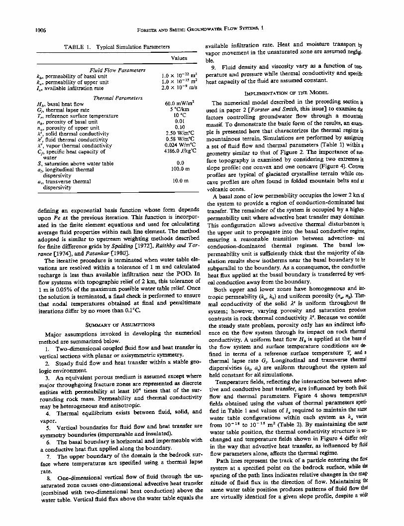
TABLE 1. Typical Simulation Parameters

Values

Fluid Flow Parameters

kt,, permeability of basal unit k,,, permeability of upper unit I•, available infiltration rate

Thermal Parameters

Ha, basal heat flow G t, thermal lapse rate Tr, reference surface temperature n•,, porosity of basal unit n,,, porosity of upper unit A•', solid thermal conductivity if, fluid thermal conductivity X *', vapor thermal conductivity C•,; specific heat capacity of

water

S, saturation above water table a•, longitudinal thermal

dispersivity a t , transverse thermal

dispersivity

1.0 x 10 -22 m 2 1.0 x 10 -15 m 2 2.0 x 10 -9 m/s

60.0 mW/m 2 5 øC/km

10 øC 0.01 0.10

2.50 W/møC 0.58 W/møC 0.024 W/møC 4186.0 J/kgøC

0.0

100.0 m

10.0 m

defining an exponential basis function whose form depends upon Pe at the previous iteration. This function is incorporated in the finite element equations and used for calculating average fluid properties within each line element. The method adopted is similar to upstream weighting methods described for finite difference grids by Spalding ['1972], Raithby and Tor- rance [1974], and Patankar [1980'1.

The iterative procedure is terminated when water table elevations are resolved within a tolerance of 1 m and calculated recharge is less than available infiltration near the POD. In flow systems with topographic relief of 2 km, this tolerance of 1 m is 0.05% of the maximum possible water table relief. Once the solution is terminated, a final check is performed to ensure that nodal temperatures obtained at final and penultimate iterations differ by no more than 0.1 øC.

SUMMARY OF ASSUMPTIONS

Major assumptions invoked in developing the numerical method are summarized below.

1. Two-dimensional coupled fluid flow and heat transfer in vertical sections with planar or axisymmetric symmetry.

2. Steady fluid flow and heat transfer within a stable geologic environment.

3. An equivalent porous medium is assumed except where major throughgoing fracture zones are represented as discrete entities with permeability at least 10 '• times that of the sur- rounding rock mass. Permeability and thermal conductivity may be heterogeneous and anisotropic.

4. Thermal equilibrium exists between fluid, solid, and vapor.

5. Vertical boundaries for fluid flow and heat transfer are symmetry boundaries (impermeable and insulated).

6. The basal boundary is horizontal and impermeable with a conductive heat flux applied along the boundary.

7. The upper boundary of the domain is the bedrock surface where temperatures are specified using a thermal lapse rate.

8. One-dimensional vertical flow of fluid through the unsaturated zone causes one-dimensional advective heat transfer (combined with two-dimensional heat conduction) above the water table. Vertical fluid flux above the water table equals the

available infiltration rate. Heat and moisture transport by vapor movement in the unsaturated zone are assumed negligi. ble.

9. Fluid density and viscosity vary as a function of tern. perature and pressure while thermal conductivity and specific heat capacity of the fluid are assumed constant.

IMPLEMENTATION OF THE MODEL

The numerical model described in the preceding section is used in paper 2 [Forster and Smith, this issue] to examine the factors controlling groundwater flow through a mountain massif. To demonstrate the basic form of the results, an exam. ple is presented here that characterizes the thermal regime in mountainous terrain. Simulations are performed by assigning a set of fluid flow and thermal parameters (Table 1) within a geometry similar to that of Figure 2. The importance of sur. face topography is examined by considering two extremes in slope profile: one convex and one concave (Figure 4). Convex profiles are typical of glaciated crystalline terrain while con. cave profiles are often found in folded mountain belts and at volcanic cones.

A basal zone of low permeability occupies the lower 2 km of the system to provide a region of conduction-dominated heat transfer. The remainder of the system is occupied by a higher. permeability unit where advective heat transfer may dominate. This configuration allows advective thermal disturbances in the upper unit to propagate into the basal conductive regime, ensuring a reasonable transition between advection-and conduction-dominated thermal regimes. The basal 10w- permeability unit is sufficiently thick that the majority of sim. ulation results show isotherms near the basal boundary to be subparallel to the boundary. As a consequence, the conductive heat flux applied at the basal boundary is transferred by vertical conduction away from the boundary.

Both upper and lower zones have homogeneous and isotropic permeability (k u, k b) and uniform porosity (n,,, nb). Ther- mal conductivity of the solid 2 s is uniform throughout the system; however, varying porosity and saturation produce contrasts in rock thermal conductivity 2 e. Because we consider the steady state problem, porosity only has an indirect influence on the flow system through its impact on rock thermal conductivity. A uniform heat flow H• is applied at the base 0f the flow system and surface temperature conditions are de fined in terms of a reference surface temperature T, and a thermal lapse rate Gv Longitudinal and transverse thermal dispersivities (a t, a t) are uniform throughout the system and held constant for all simulations.

Temperature fields, reflecting the interaction between advective and conductive heat transfer, are influenced by both fluid flow and thermal parameters. Figure 4 shows temperature fields obtained using the values of thermal parameters specified in Table i and values of I z required to maintain the same water table configurations within each system as k u varies from !0- • to 10- x• m 2 (Table 2). By maintaining the same water table position, the thermal conductivity structure is unchanged and temperature fields shown in Figure 4 differ only in the way that advective heat transfer, as influenced by fluid flow parameters alone, affects the thermal regime.

Path lines represent the track of a particle entering the ft0w system at a specified point on the bedrock surface, while the spacing of the path lines indicates relative changes in the magnitude of fluid flux in the direction of flow. Maintaining the same water table position produces patterns of fluid flow that are virtually identical for a given slope profile, despite a wide

FORSTER ̂ND SMITH' GROUNDWATER FLOW SYS•MS, 1 1007

,>,,

Run C1

Run C3

0 2 4 6

DISTANCE (km)

Run C2

Run C4

0 2 4 6

DISTANCE (km)

Run B2

i ................. i

Run B7

.. :::::::::::::::::::::::::::::::::::::::::::::::::::::::: ::::::::::::::::::::::::::::::::::::::::::::::::::::::::

0 2 4 6

DISTANCE (km)

.... -•- Groundwater pathline

--5--.• Isotherm (øC) Water table

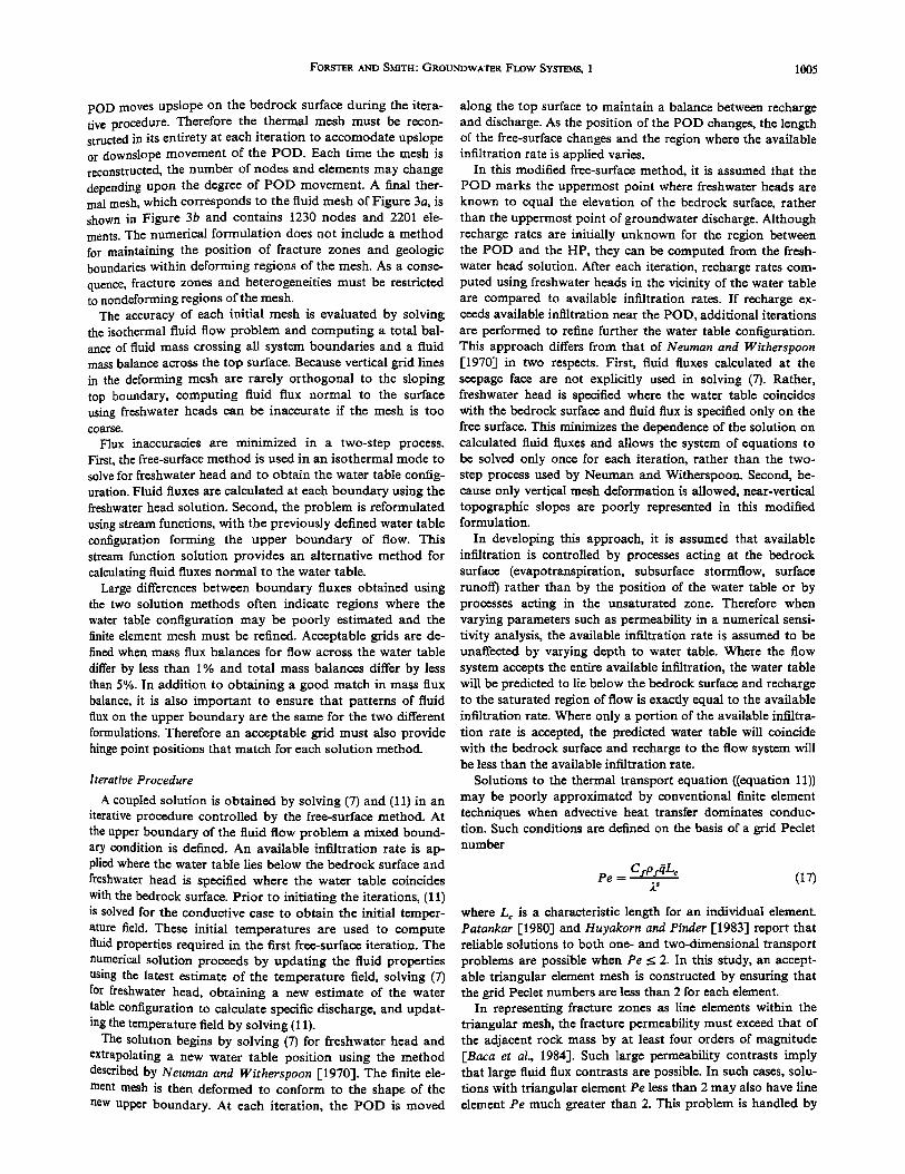
Fig. 4. Temperature fields and groundwater flow patterns as a function of upper zone permeability k, for fixed water table configurations in concave and convex slope profiles: (a) k, = 10 -x8 m 2 (I= = 2 x 10-x2 m/s for convex run C1 and 5 x 10 -•2 m/s for concave run C3); (b) k u = 10 -t6 m 2 (I•. = 2 x 10 -•ø m/s for convex run C2 and 5 x 10 -tø m/s for concave run C4); and (c) k,, = I0- • m 2 (I= = 2 x 10 -9 m/s for convex run B2 and 5 x 10 -9 m/s for concave run B7).

variation in the temperature fields. Despite their obvious simi- larry, path lines should not be confused with the streamlines generated from contour plots of a suitably defined stream function or velocity potential. These approaches differ because fluid flow through each streamtube (bounded by each pair of path lines) is fixed throughout the domain while fluid flow through flow tubes defined on the basis of path lines may differ from flow tube to flow tube.

Water table configurations are maintained by increasing I• by the same increment that k, is increased. Maintaining the water table position as permeability is increased implies that increasingly humid climates support the increased infiltration rates. The relationship between infiltration rate, permeability, and water table elevation is examined in detail in paper 2 [Forster and Smith, this issue].

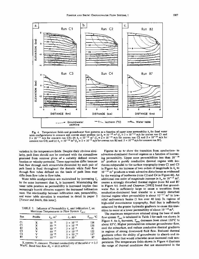
TABLE 2. Influence of Permeability k,, and Infiltration I, on Maximum Temperatures in Flow System Tma, •

Run Profile k,,, m 2 I z, m/s Tm..x, øC

CI X 10 -•8 2 X 10 -12 138 C2 X 10 -]6 2 x !0 -•ø 130 B2 X 10-]5 2 X 10 -9 81 C3 V 10 -!8 5 X 10 -12 122 C4 V 10 -]6 5 x 10 -•ø 117 B7 V 10 -•5 5 X 10 -9 87

X, convex: V, concave. Thermal conductivity of the solid A'" = 2.5 W o /rn C. Basal heat flow H•, 60.0 mW/m 2.

Figures 4a to 4c show the transition from conduction- to advection-dominated thermal regimes as a function of increasing permeability. Upper zone permeabilities less than 10- • m 2 produce a purely conductive thermal regime with isotherms subparallel to the surface topography (runs C! and C3 in Figure 4a). An increase of two orders of magnitude in k,, to 10- •6 m • produces a weak advective disturbance as evidenced by the warping of isotherms (runs C2 and C4 in Figure 4b). An additional one order of magnitude increase in k,, to 10- • m 2, creates a strongly disturbed thermal regime (runs B2 and B7 in Figure 4c). Smith and Chapman E1983] found that groundwater flux is sufficiently large to cause a transition from conduction-dominated heat transfer to a weakly disturbed thermal regime when permeability is about 10- • v m •' in low- relief sedimentary basins (1 km over 40 km). In regions of high-relief mountainous topography, fluid flux is sufficiently enhanced by the greater hydraulic gradients to cause this transition to occur at a lower permeability of about 10- • m 2.

The maximum temperature attained along the base of each flow system Tm• • is tabulated in Table 2 for each run shown in Figure 4. As k. increases, Tmax decreases from about 130øC to about 85øC. Higher permeabilities enhance groundwater flow, cool the subsurface, and reduce conductive thermal gradients in regions of strong downward fluid flow. Reduced thermal gradients reflect the ability of groundwater to absorb and re- distribute heat that would otherwise cause increased rock temperatures. The temperature fields shown in Figure 4 illustrate the range of thermal conditions that are encountered in the

1008 FOmSTœR AND SMITH: Gt<OUNDWATER FLOW SYSTEMS, 1

sensitivity analyses carried out in paper 2 [Forster and Smith, this issue].

trolled as an input variable rather than implicitly calculated in the solution procedure.

SUMMARY

1. Groundwater flow systems in mountainous terrain differ from those in low-relief terrain in two key respects: (1) for a given set of hydrogeologic conditions, a greater range in water table elevation and form is possible; (2) high-relief terrain enhances groundwater circulation to depths where significant heating can occur, implying that thermal effects influence the patterns and rates of groundwater flow.

2. A conceptual model has been outlined to describe groundwater flow and thermal regimes in mountainous terrain. The uppermost boundary of the domain is the bedrock surface. Where the water table coincides with the bedrock

surface, freshwater head equals the bedrock elevation. Where the water table lies below the bedrock surface, a uniform available infiltration rate is applied that is transmitted directly to the water table by one-dimensional flow through the unsaturated zone. Heat supplied by a regional heat flux is transferred through the system by advection and conduction in both saturated and unsaturated regions of flow. Fluid flow and heat transfer through a thin cover of discontinuous surficial deposits on upland areas of mountain slopes is not included in the model. Fluid moving within these deposits is lumped with overland flow as a runoff term. The remaining fluid available for recharge is termed an available infiltration rate that in the absence of detailed field data, is best thought of as a percentage of the mean annual precipitation rate.

3. Traditional free-surface approaches incorrectly assume that recharge cannot occur downslope of the point where the water table meets the bedrock surface (commonly defined as the exit point marking the upper limit of the seepage face). In developing the approach used in this study, it was necessary to identify two separate points on the upper boundary; the point where the water table meets the bedrock surface (POD) and the point that marks the transition between recharge and discharge (HP). Between these points the water table coincides with the bedrock surface. In this region, the boundary condition is specified by setting hydraulic head equal to the elevation of the upper boundary and allowing recharge to occur at a rate defined by the nature of the groundwater flow system. In steep terrain, with rocks of low permeability, recharge can occur downslope of the POD in a region that might normally be considered part of the seepage face. In regions of reduced topographic relief, the separation between HP and POD becomes smaller and these points merge at the commonly defined exit point.

4. The fluid and thermal regimes are modeled using a Ga- lerkin finite element technique in conjunction with a free- surface approach to estimate the position of the water table. Two finite element grids are required in solving this problem. The mesh for fluid flow is generated only within the saturated zone. The mesh for heat transfer extends from the basal

boundary to the bedrock surface, incorporating both saturated and unsaturated regions of flow. Coupling between heat transfer and fluid flow is facilitated by ensuring a one-to-one correspondence between nodes located below the water table.

5. The numerical method developed in this paper provides the means to examine the factors that control groundwater flow and heat transfer in mountainous terrain: geology, surface topography, climate, and regional heat flow. It is advanta- geous to adopt the flee-surface approach when performing sensitivity analyses because recharge to the flow system is con-

APPENDIX: DISTINCTION BETWEEN POINT OF DETACHMI•NT AND HINGE POINT ON A SEEPAGE FACE

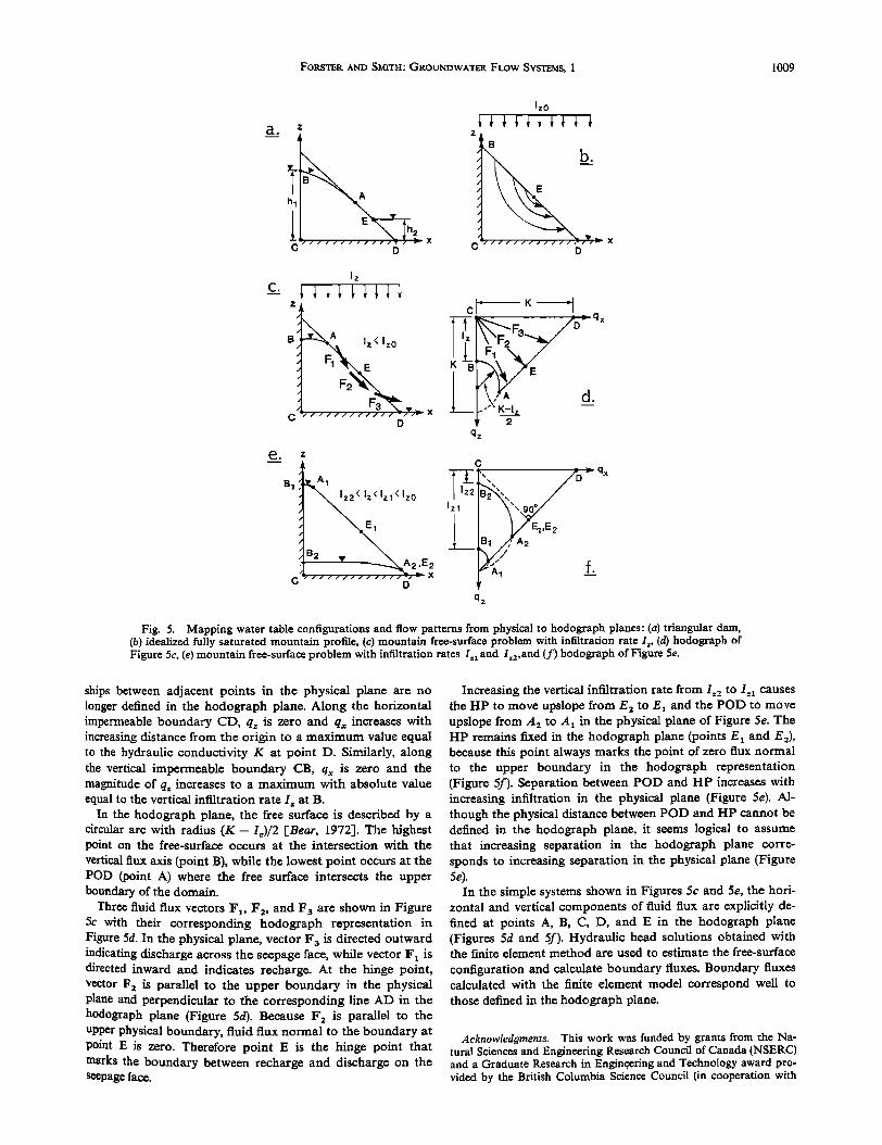
Conventional approaches to solving free-surface ground. water flow problems assume that a single point, the exit point, marks the boundary between the free-surface and the seepage face. Two conditions occur at this point: the free-surface de. viates from the seepage face, and the upper limit of discharge on the seepage face is defined. These conditions occur at a single point for free-surface problems similar to the triangular earthen dam shown in Figure 5a. In this isothermal example, a homogeneous isotropic hydraulic conductivity K is assumed for all panels shown in Figure 5. The horizontal base CD is impermeable while segments BC and DE are constant head boundaries with head differential •Sh = h•- h 2. The form of free-surface AB, the length of the seepage face AE and the position of the exit point A are controlled by this head differ. ential, the geometry of the dam, the hydraulic conductivity K, and the pattern of infiltration applied on the upper surface 0f the dam.

In a simplified mountain groundwater flow problem, the vertical left-hand boundary of Figure 5a becomes a symmetry boundary (Figure 5b). At a high uniform infiltration rate the water table coincides with the ground surface across the flow system. In this case, a free surface is absent and the entire upper surface can be considered a seepage face. The HP at point E on the seepage face marks the boundary between recharge and discharge and fulfills one condition of an exit point by defining the upper limit of discharge. The point detachment A is undefined in Figure 5b because a free surface is absent under conditions where the water table is everywhere at the bedrock surface. Reducing the infiltration rate to I., causes a free surface to develop (Figure 5c) with POD at A and a HP at E. In this case, a single point cannot be defined that fulfills the definition of an exit point and recharge may occur on the seepage face between the POD and HP. Further reducing the infiltration rate decreases the separation between POD and HP (A and E). In low-relief topography, the separation becomes negligible and the usual exit point definition is valid. in high-relief mountainous topography, the separation between POD and HP can be substantial and must be considered in the numerical formulation.

Bear [1972, pg. 272] notes that mapping free-surface groundwater flow problems into the hodograph plane is a useful method for examining flow conditions at the boundaries. While the boundary between the free surface and the seepage face is initially unknown in the physical plane, in the hodograph plane it is completely defined. This mapping procedure provides an analytical argument that supports the concept of separated POD and HP on seepage faces in mountainous terrain. Details on methods of mapping from the physical to hodograph planes can be found in the work by Bear [1972] and Verruijt [1970].

Figure 5d is the hodograph representation of the physical system of Figure 5c. In the hodograph plane, vertical and horizontal components of fluid flux (qz, q,•) at each point on the boundary of the physical system form the hodograph. The outline of the hodograph is defined as the locus of points marking the distal ends of specific discharge vectors originat- ing at point C (see vectors F•, F 2, and F 3 shown in Figures 5c and 5d). In the mapping process, however, the spatial relation-

FO]•STE]• AND SMITH: GROUNDWATER FLOW SYSTEMS, 1 1009

ao

½ D

Iz0

b / E

/

D

C,

e.

/

/

/

/

J

/

/

c

[z

•%• I z < I z0

D

z

B 1 5 A-"•2 < • Iz<lzl<lz0 /

/

/

/ E 1 /

/

/

/

ß ' x 2 c•' D

qz

c

V El'E2 B1 /½r/A2

qz

Fig. 5. Mapping water table configurations and flow patterns from physical to hodograph planes: (a) triangular dam, (b) idealized fully saturated mountain profile, (c) mountain free-surface problem with infiltration rate I_., (d) hodograph of Figure 5c, (e) mountain free-surface problem with infiltration rates I:z and I=2, and (f) hodograph of Figure 5e.

ships between adjacent points in the physical plane are no longer defined in the hodograph plane. Along the horizontal impermeable boundary CD, q.. is zero and qx increases with increasing distance from the origin to a maximum value equal to the hydraulic conductivity K at point D. Similarly, along the vertical impermeable boundary CB, qx is zero and the magnitude of q.. increases to a maximum with absolute value equal to the vertical infiltration rate I s at B.

In the hodograph plane, the free surface is described by a circular arc with radius (K- I•)/2 [Bear, 1972]. The highest point on the free-surface occurs at the intersection with the vertical flux axis (point B), while the lowest point occurs at the POD (point A) where the free surface intersects the upper boundary of the domain.

Three fluid flux vectors Fx, F 2, and F 3 are shown in Figure 5c with their corresponding hodograph representation in Figure 5d. In the physical plane, vector F 3 is directed outward indicating discharge across the seepage face, while vector F x is directed inward and indicates recharge. At the hinge point, vector F 2 is parallel to the upper boundary in the physical plane and perpendicular to the corresponding line AD in the hodograph plane (Figure 5d). Because F 2 is parallel to the upper physical boundary, fluid flux normal to the boundary at point E is zero. Therefore point E is the hinge point that marks the boundary between recharge and discharge on the seepage face.

Increasing the vertical infiltration rate from Iz2 to I..• causes the HP to move upslope from E 2 to E• and the POD to move upslope from A 2 to A 1 in the physical plane of Figure 5e. The HP remains fixed in the hodograph plane (points E x and E2), because this point always marks the point of zero flux normal to the upper boundary in the hodograph representation (Figure 5f). Separation between POD and HP increases with increasing infiltration in the physical plane (Figure 5e). Al- though the physical distance between POD and HP cannot be defined in the hodograph plane, it seems logical to assume that increasing separation in the hodograph plane corresponds to increasing separation in the physical plane (Figure 5e).

In the simple systems shown in Figures 5c and 5e, the horizontal and vertical components of fluid flux are explicitly defined at points A, B, C, D, and E in the hodograph plane (Figures 5d and 5f). Hydraulic head solutions obtained with the finite element method are used to estimate the free-surface

configuration and calculate boundary fluxes. Boundary fluxes calculated with the finite element model correspond well to those defined in the hodograph plane.

Acknowledgments. This work was funded by grants from the Na- tural Sciences and Engineering Research Council of Canada (NSERC) and a Graduate Research in Engine, ering and Technology award pro- vided by the British Columbia Science Council {in cooperation with

1010 FORST•-R AND SMITH: GROUNDWATER FX. OW SYSTEMS, 1

Nevin Sadlief-Brown Goodbrand Company Limited). Discussions with David Chapman are gratefully acknowledged. Thanks are also extended to Allan Freeze for reviewing the manuscript and sharing his views on the development of seepage faces in mountainous terrain. Gedeon Dagan is to be thanked for providing an illuminating discussion of hodograph methods. Computations were carried out on an FPS 164 MAX Array Processor supported by an NSERC Major Installation Grant to the University of British Columbia.

REFERENCES

Adams, M. C., J. N. Moore, and C. B. Forster, Fluid flow in volcanic terrains--Hydrogeochemistry of the Meager Mountain thermal system, Geotherm. Resour. Counc. Trans., 9, 377-382, 1985.

Baca, R. G., R. C. Arnett, and D. W. Langford, Modelling fluid flow in fractured-porous rock masses by finite element techniques, lnt. J. Numer. Methods Fluids, 4, 337-348, 1984.

Barry, R. G., Mountain Weather and Climate, Methuen, London, I981.

Bear, J., Dynamics of Fluids in Porous Media, Elsevier Science, New York, 1972.

Bear, J., Hydraulics of Groundwater, McGraw-Hill, New York, 1979. Birch, F., Flow of heat in the Front Range, Colorado, Geol. $oc. Am.

Bull., 61, 567-630, i950. Blackwell, D. D., and J. L. Steele, A summary of heat flow studies in

the Cascade Range, Geotherm. Resour. Counc. Trans., 7, 233-236, 1983.

Bodvarsson, G. S., and K. Pruess, Modeling studies of geothermal systems with a free water surface, Rep. LBL-17146, 8 pp., Lawrence Berkeley Lab., Univ. of Calif., Berkeley, 1983.

Bortolami, G. S., B. Ricci, G. G. Susella, and G. M. Zuppi, Hy- drogeochemistry of the Corsaglia Valley, Maritime Alps Piedmont Italy, J. Hydrol., 44, 57-79, 1979.

Chapman, D. S., and L. Rybach, Heatflow anomalies and their interpretation, J. Geodyn., 4, 3-37, 1985.

Forster, C. B., and L. Smith, Groundwater flow systems in mountainous terrain, 2, Controlling factors, Water Resour. Res., this issue.

Fox, F. M., The Simplon tunnel, Minutes Proc. Inst. Civ. En#., 168, 61-86, 1907.

Freeze, R. A., and P. A. Witherspoon, Theoretical analysis of regional groundwater flow, 2, Effect of water table configuration and subsurface permeability variation, Water Resour. Res., 3, 623-634, 1967.

Frind, E. O., Simulations of long-term transient density-dependant transport in groundwater, Adv. Water Resour., 5, 73-88, 1982.

Halstead, E. C., Groundwater investigation, Mount Kobau, British Columbia, Tech. Butt., 17, Canada Inland Waters Branch, Dep. of Energy Mines and Resour., Ottawa, 1969.

Hennings, F., On the question of long railway tunnels. Construction, ventilation and operation, Bull. Int. Railway Con•7ress Assoc., 24(10), 943-983, 1910.

Horne, R. N., and M. J. O'Sullivan, Numerical modeling of a desatu- rating geothermal reservoir, Numer. Heat Transfer, 1, 203-216, 1978.

Huyakorn, P.S., and G. F. Pinder, Computational Methods in $ubsur- .face Flow, Academic, Orlando, Fla., 1983.

Ingebritsen, S. E., and M. L. Sorey, A quantitative analysis of the Lassen hydrothermal system, North Central California, Water Resour. Res., 2•(6), 853-868, 1985.

Jamier, D., Etude de la fissuration, de l'hydrogeologie et de la ochemie des eaux profondes des massifs de l'Arpille et du Mont Blanc, Ph.D. dissertation, Faculte des Sci., Univ. de Neuchatel, Switzerland, 1975.

Jamieson, G. R., and R. A. Freeze, Determining hydraulic conductivity distributions in a mountainous area using mathematical mod-

eling, Groundwater, 21(2), 168-177, 1983. Keays, R. N., Construction methods in the Moffat Tunnel, Trans. Am.

Soc. Civ. En!7., 62, 63-112, 1928. Keenan, J. H., F. G. Keyes, P. G. Hill, and J. G. Moore, Steam

Tables, 162 pp., John Wiley, New York, 1978.

Lahsen, A., and P. Trujillo, The geothermal field of El Tatio, Chile, in Proc. 2nd. U.N. Syrup. on Development and Use of Geothermal Re. sources, vol. 1, pp. 157-175, U.S. Government Printing Office, San Francisco, Calif., 1975.

Martinec, J., H. Oeschager, U. Schotterer, and U. Siegenthaler, Snow. melt and groundwater storage in an alpine basin, Hydrological Aspects of Alpine and High Mountainous Terrain, IAH$ Publ., 138, 169-175, 1982.

Mears, F., The eight mile Cascade Tunnel, Great Northern Railway• I!, Surveys, construction methods and a comparison of routes, Trans. Am. Soc. Civ. Ent•., 96, 915-1004, 1932.

Neuman, S. P., and P. A. Witherspoon, Finite element method of analyzing steady seepage with a free-surface, Water Resour. Res., 6(3), 889-897, 1970.

Patankar, S. V., Numerical Heat Transfer and Fluid Flow, McGraw. Hill, New York, 1980.

Raithby, G. D., and K. E. Torrance, Upstream weighting differencing schemes and their application to elliptic problems involving fluid flow, Comp. Fluids, 2, 191-206, 1974.

Ross, B., A conceptual model of deep unsaturated zones with negligible recharge, Water Resour. Res., 20(11), 1627-1629, 1984.

Sauty, J.P., A. C. Gringarten, H. Fabris, D. Thiery, A. Menjoz, and ?. A. Landel, Sensible energy storage in aquifers, 2, Field experiments and comparisons with theoretical results, Water Resour. Res., I8121, 245-252, 1982.

Schardt, M. H., Les resultats scientifique• du percement du tunnel du Simplon, Bull. Tech. Suisse Romande, 31, 125-178, 1905.

Scharli, U., and L. Rybach, On the thermal conductivity of !0w. porosity crystalline rocks, Tectonophysics, 103, 307-313, 1984.

Sklash, M. G., and R. N. Farvolden, The role of groundwater in storm runoff, J. Hydrol., 43, 45-65, 1979.

Smart, C. C., The hydrology of the Castleguard Karst, Columbia Icefields, Alberta, Canada, Arctic Alpine Res., 15(4), 471-486, 1985.

Smith, L., and D. S. Chapman, On the thermal effects of groundwater flow, 1, Regional scale systems, J. Geophys. Res., 88(B1), 593-608, 1983.

Sorey, M. L., Numerical modeling of liquid geothermal systems, U.S. Geol. Surv. Prof. Pap., 1044-D, 1978.

Sorey, M. L., Types of hydrothermal convection systems in the Cas- cade Range of California and Oregon, U.S. Geol. Surv. Open File Rep., 85-521, 1985.

Spalding, D. B., A novel finite difference formulation for differential equations involving both first and second derivatives, Int. J. Numer. Methods En•., 4, 551-559, 1972.

Thompson, W. T., How and why to distinguish between mountains and hills, Prof. Geotjr., 16, 6-8, 1964.

Verruijt, A., Theory of Groundwater Flow, Macmillan, New York, 1970.

Walsh, J. B., and E. R., Decker, Effect of pressure and saturating fluid on the thermal conductivity of compact rock, J. Geophys. Res., 71, 3053-3061, 1966.

Watson, J. T. R., R. J. Basu, and J. V. Sengers, An improved representative equation for the dynamic viscosity of water substance, Z Phys. Chem. Ref. Data, 9(3), 1255-1279, 1981.

Zablocki, C. J., R. I. Tilling, D. W. Peterson, R. L. Christiansen, G. V. Keller, and J. C. Murray, A deep research hole at the summit of an active volcano, Kilauea, Hawaii, Geophys. Res. Lett., 1(7), 323-326, 1974.

C. Forster, Department of Geology, Utah State University, Logan, UT 84322.

L. Smith, Department of Geological Sciences, University of British Columbia, Vancouver, British Columbia, Canada V6T 2B4.

(Received July 8, 1987; revised January 25, 1988;

accepted January 26, 1988.)

Documents

Groundwater Flow Systems in Mountainous Terrain 1