1

Ground Investigation in Urban Environment:

Based on Seismic Methods: Analysis of the

influence of the boundary conditions

Rodrigo Silva Baptista

Department of Civil Engineering and Architecture and Georesources, IST, University of Lisbon September 2016

Abstract:

This work presents the joint analysis of two geophysical tests, the MASW (Multichannel

Acquisition of Surface Waves) and the HVSR (Horizontal to Vertical Spectral Ratio) in highly

dense urban areas and assess their applicability when underground infrastructures are in the

vicinity.

A case study located in central Lisbon is analyzed. Data from boreholes and SPT tests

and from MASW and HVSR were used to build a geological-geotechnical model. Afterwards the

numerical simulation of the MASW test was carried out and results where compared with the

experimental data. Validation of the model was achieved when both results showed to be in good

agreement. Then, the effect of the presence of underground structures was evaluated.

The results showed small interference on the dispersion curve due to the presence of

underground structures, mainly in the low frequency range.

Keywords: MASW, HVSR, finite difference method, wave propagation, small-strain stiffness

1 Motivation

Assessing soil properties with a low degree of

uncertainty and knowing their spacial variability are a

fundamental aspect for every geotechnical engineer.

Seismic methods based on surface waves to

characterize the soil stiffness in the small strain range is

important for seismic site effects prediction.

Numerical software, such as FLAC, are ofter used

to study complex geotechnical problems. Knowing their

advantages and limitations is a stepping stone for a

careful modelling and for an accurate analysis of the

problem at hand.

2 Objectives

This work focuses on analysing the joint application

of two seismic methods, the MASW and the HVSR

when underground structures are in the vicinity

comparing results from a case study through numerical

simulation.

3 Methods

Firstly, numerical modelling considering plane

strain is used to check the reliability of the numerical

tools to accurately simulate wave propagation problems

for a case of unidimensional wave propagation on a

homogeneous soil column.

Secondly a case study is modelled and validated

when both the MASW field results and the numerical

2

MASW match. Finally, underground structures are

introduced in the model and the differences between

numerical results are analysed.

4 Seismic Tests

Two seismic tests were used in this study, the

MASW and the HVSR. Both tests are based on the

surface wave method, which takes advantage of the

Rayleigh wave characteristics and its propagation to

determine the soil properties although their acquisition

and processing tools differ.

4.1 MASW

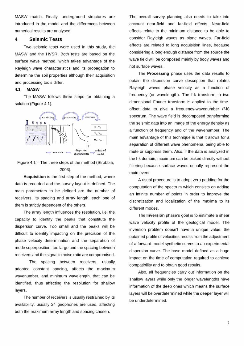
The MASW follows three steps for obtaining a

solution (Figure 4.1).

Figure 4.1 – The three steps of the method (Strobbia,

2003).

Acquisition is the first step of the method, where

data is recorded and the survey layout is defined. The

main parameters to be defined are the number of

receivers, its spacing and array length, each one of

them is strictly dependent of the others.

The array length influences the resolution, i.e. the

capacity to identify the peaks that constitute the

dispersion curve. Too small and the peaks will be

difficult to identify impacting on the precision of the

phase velocity determination and the separation of

mode superposition, too large and the spacing between

receivers and the signal to noise ratio are compromised.

The spacing between receivers, usually

adopted constant spacing, affects the maximum

wavenumber, and minimum wavelength, that can be

identified, thus affecting the resolution for shallow

layers.

The number of receivers is usually restrained by its

availability, usually 24 geophones are used, affecting

both the maximum array length and spacing chosen.

The overall survey planning also needs to take into

account near-field and far-field effects. Near-field

effects relate to the minimum distance to be able to

consider Rayleigh waves as plane waves. Far-field

effects are related to long acquisition lines, because

considering a long enough distance from the source the

wave field will be composed mainly by body waves and

not surface waves.

The Processing phase uses the data results to

obtain the dispersion curve description that relates

Rayleigh waves phase velocity as a function of

frequency (or wavelength). The f-k transform, a two

dimensional Fourier transform is applied to the time-

offset data to give a frequency-wavenumber (f-k)

spectrum. The wave field is decomposed transforming

the seismic data into an image of the energy density as

a function of frequency and of the wavenumber. The

main advantage of this technique is that it allows for a

separation of different wave phenomena, being able to

mute or suppress them. Also, if the data is analyzed in

the f-k domain, maximum can be picked directly without

filtering because surface waves usually represent the

main event.

A usual procedure is to adopt zero padding for the

computation of the spectrum which consists on adding

an infinite number of points in order to improve the

discretization and localization of the maxima to its

different modes.

The Inversion phase’s goal is to estimate a shear

wave velocity profile of the geological model. The

inversion problem doesn’t have a unique value: the

obtained profile of velocities results from the adjustment

of a forward model synthetic curves to an experimental

dispersion curve. The base model defined as a huge

impact on the time of computation required to achieve

compatibility and to obtain good results.

Also, all frequencies carry out information on the

shallow layers while only the longer wavelengths have

information of the deep ones which means the surface

layers will be overdetermined while the deeper layer will

be underdetermined.

3

4.2 HVSR

The HVSR is a method proposed by Nakamura

(2000) based on the spectral ratio between the

horizontal and vertical components of ambient noise

recorded at the surface. Its main objective is to estimate

the value of the fundamental frequency of soft soils.

It is a passive method, requiring no active source

to be applied but with longer acquisition time, taking

advantage of the properties of the elipticity and phase

velocity of Rayleigh waves when they interact with

layers of different stiffness.

The elipticity is also a function of the frequency, if

stiffness contrasts between layers are present, the H/V

curve will exhibit peaks (maximums) due to the

nullification of the vertical component and minimums

when the horizontal component nullifies. If the stiffness

contrast is high enough, infinite maximums and zeros

are detected and also a reversal of the movement of the

particles from retrograde to progressive.

The frequency at which the curve exhibits peaks is

close to the fundamental frequency of the S waves,

which indicates the overall fundamental frequency of

the deposits. An estimate of the amplification factor can

also be obtained analysing the peaks value, although

the method tends to underestimate it.

This method can provide a way for detection of the

depth of the bedrock and an indicator of the degree of

stiffness of the soil deposit since it relies on

considerable stiffness contrast, usually located on the

interface between the bedrock and the soil deposits.

Project SESAME, elaborated by Bard et al. (2004)

designed some recommended procedures regarding

survey layout, number of tests, time of day, etc. in order

to retrieve the best possible results from the location.

5 Case Study

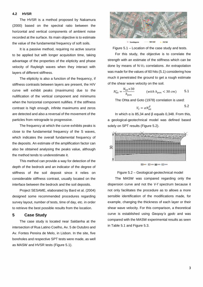
The case study is located near Saldanha at the

intersection of Rua Latino Coelho, Av. 5 de Outubro and

Av. Fontes Pereira de Melo, in Lisbon. In the site, five

boreholes and respective SPT tests were made, as well

as MASW and HVSR tests (Figure 5.1).

Figure 5.1 – Location of the case study and tests.

For this study, the objective is to correlate the

strength with an estimate of the stiffness which can be

done by means of N-VS correlations. An extrapolation

was made for the values of 60 hits (5.1) considering how

much it penetrated the ground to get a rough estimate

of the shear wave velocity on the soil.

𝑁60∗ =

𝑁60×30

ℎ𝑝𝑒𝑛

(𝑤𝑖𝑡ℎ ℎ𝑝𝑒𝑛 < 30 𝑐𝑚) 5.1

The Ohta and Goto (1978) correlation is used:

𝑉𝑆 = 𝛼𝑁60𝛽

5.2

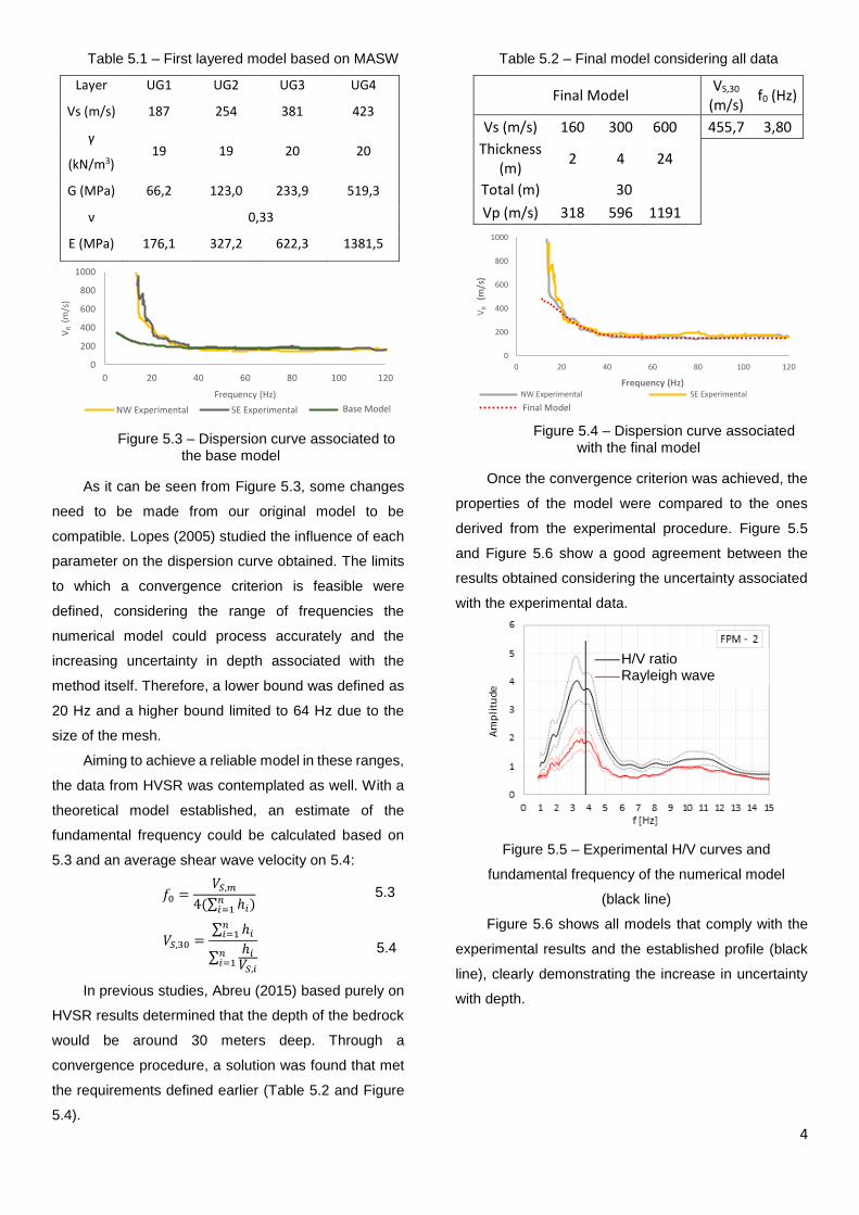
In which α is 85,34 and β equals 0,348. From this,

a geological-geotechnical model was defined based

solely on SPT results (Figure 5.2).

Figure 5.2 – Geological-geotechnical model

The MASW was compared regarding only the

dispersion curve and not the V-f spectrum because it

not only facilitates the procedure as to allows a more

sensible identification of the modifications made, for

example, changing the thickness of each layer or their

shear wave velocity. For this comparison, a theoretical

curve is established using Geopsy’s gpdc and was

compared with the MASW experimental results as seen

in Table 5.1 and Figure 5.3.

4

Table 5.1 – First layered model based on MASW

Layer UG1 UG2 UG3 UG4

Vs (m/s) 187 254 381 423

γ

(kN/m3) 19 19 20 20

G (MPa) 66,2 123,0 233,9 519,3

ν 0,33

E (MPa) 176,1 327,2 622,3 1381,5

Figure 5.3 – Dispersion curve associated to the base model

As it can be seen from Figure 5.3, some changes

need to be made from our original model to be

compatible. Lopes (2005) studied the influence of each

parameter on the dispersion curve obtained. The limits

to which a convergence criterion is feasible were

defined, considering the range of frequencies the

numerical model could process accurately and the

increasing uncertainty in depth associated with the

method itself. Therefore, a lower bound was defined as

20 Hz and a higher bound limited to 64 Hz due to the

size of the mesh.

Aiming to achieve a reliable model in these ranges,

the data from HVSR was contemplated as well. With a

theoretical model established, an estimate of the

fundamental frequency could be calculated based on

5.3 and an average shear wave velocity on 5.4:

𝑓0 =𝑉𝑆,𝑚

4(∑ ℎ𝑖)𝑛𝑖=1

5.3

𝑉𝑆,30 =∑ ℎ𝑖

𝑛𝑖=1

∑ℎ𝑖

𝑉𝑆,𝑖

𝑛𝑖=1

5.4

In previous studies, Abreu (2015) based purely on

HVSR results determined that the depth of the bedrock

would be around 30 meters deep. Through a

convergence procedure, a solution was found that met

the requirements defined earlier (Table 5.2 and Figure

5.4).

Table 5.2 – Final model considering all data

Final Model VS,30

(m/s) f0 (Hz)

Vs (m/s) 160 300 600 455,7 3,80

Thickness (m)

2 4 24

Total (m) 30

Vp (m/s) 318 596 1191

Figure 5.4 – Dispersion curve associated with the final model

Once the convergence criterion was achieved, the

properties of the model were compared to the ones

derived from the experimental procedure. Figure 5.5

and Figure 5.6 show a good agreement between the

results obtained considering the uncertainty associated

with the experimental data.

Figure 5.5 – Experimental H/V curves and

fundamental frequency of the numerical model

(black line)

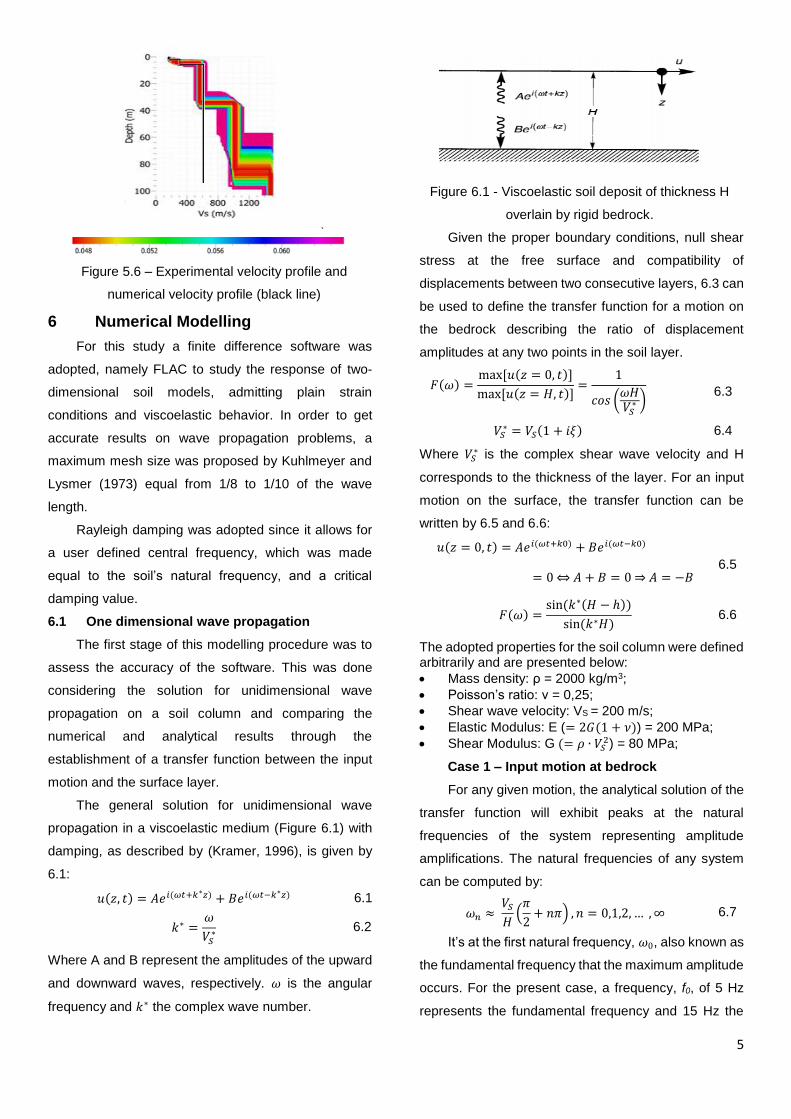
Figure 5.6 shows all models that comply with the

experimental results and the established profile (black

line), clearly demonstrating the increase in uncertainty

with depth.

0

200

400

600

800

1000

0 20 40 60 80 100 120

VR

(m

/s)

Frequency (Hz)

NW Experimental SE Experimental Teórica 1

0

200

400

600

800

1000

0 20 40 60 80 100 120

VR

(m

/s)

Frequency (Hz)NW Experimental SE Experimental

Curva Dispersão Modelo Final

H/V ratio Rayleigh wave

elipticity

Base Model Final Model

5

Figure 5.6 – Experimental velocity profile and

numerical velocity profile (black line)

6 Numerical Modelling

For this study a finite difference software was

adopted, namely FLAC to study the response of two-

dimensional soil models, admitting plain strain

conditions and viscoelastic behavior. In order to get

accurate results on wave propagation problems, a

maximum mesh size was proposed by Kuhlmeyer and

Lysmer (1973) equal from 1/8 to 1/10 of the wave

length.

Rayleigh damping was adopted since it allows for

a user defined central frequency, which was made

equal to the soil’s natural frequency, and a critical

damping value.

6.1 One dimensional wave propagation

The first stage of this modelling procedure was to

assess the accuracy of the software. This was done

considering the solution for unidimensional wave

propagation on a soil column and comparing the

numerical and analytical results through the

establishment of a transfer function between the input

motion and the surface layer.

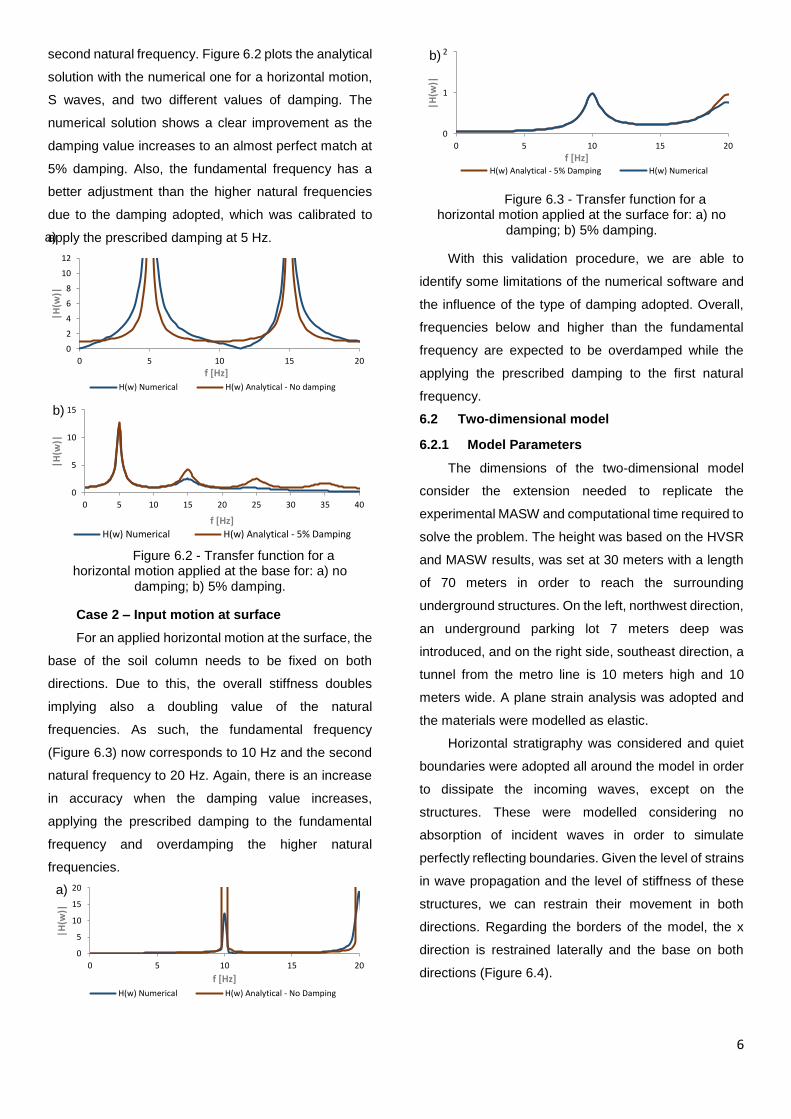
The general solution for unidimensional wave

propagation in a viscoelastic medium (Figure 6.1) with

damping, as described by (Kramer, 1996), is given by

6.1:

𝑢(𝑧, 𝑡) = 𝐴𝑒𝑖(𝜔𝑡+𝑘∗𝑧) + 𝐵𝑒𝑖(𝜔𝑡−𝑘∗𝑧) 6.1

𝑘∗ =𝜔

𝑉𝑆∗ 6.2

Where A and B represent the amplitudes of the upward

and downward waves, respectively. 𝜔 is the angular

frequency and 𝑘∗ the complex wave number.

Figure 6.1 - Viscoelastic soil deposit of thickness H

overlain by rigid bedrock.

Given the proper boundary conditions, null shear

stress at the free surface and compatibility of

displacements between two consecutive layers, 6.3 can

be used to define the transfer function for a motion on

the bedrock describing the ratio of displacement

amplitudes at any two points in the soil layer.

𝐹(𝜔) =max [𝑢(𝑧 = 0, 𝑡)]

max [𝑢(𝑧 = 𝐻, 𝑡)]=

1

𝑐𝑜𝑠 (𝜔𝐻𝑉𝑆

∗ )

6.3

𝑉𝑆∗ = 𝑉𝑆(1 + 𝑖𝜉) 6.4

Where 𝑉𝑆∗ is the complex shear wave velocity and H

corresponds to the thickness of the layer. For an input

motion on the surface, the transfer function can be

written by 6.5 and 6.6:

𝑢(𝑧 = 0, 𝑡) = 𝐴𝑒𝑖(𝜔𝑡+𝑘0) + 𝐵𝑒𝑖(𝜔𝑡−𝑘0)

= 0 ⇔ 𝐴 + 𝐵 = 0 ⇒ 𝐴 = −𝐵 6.5

𝐹(𝜔) =sin (𝑘∗(𝐻 − ℎ))

sin (𝑘∗𝐻) 6.6

The adopted properties for the soil column were defined arbitrarily and are presented below:

Mass density: ρ = 2000 kg/m3;

Poisson’s ratio: ν = 0,25;

Shear wave velocity: VS = 200 m/s;

Elastic Modulus: E (= 2𝐺(1 + 𝜈)) = 200 MPa;

Shear Modulus: G (= 𝜌 ∙ 𝑉𝑆2) = 80 MPa;

Case 1 – Input motion at bedrock

For any given motion, the analytical solution of the

transfer function will exhibit peaks at the natural

frequencies of the system representing amplitude

amplifications. The natural frequencies of any system

can be computed by:

𝜔𝑛 ≈ 𝑉𝑆

𝐻(

𝜋

2+ 𝑛𝜋) , 𝑛 = 0,1,2, … , ∞ 6.7

It’s at the first natural frequency, 𝜔0, also known as

the fundamental frequency that the maximum amplitude

occurs. For the present case, a frequency, f0, of 5 Hz

represents the fundamental frequency and 15 Hz the

6

second natural frequency. Figure 6.2 plots the analytical

solution with the numerical one for a horizontal motion,

S waves, and two different values of damping. The

numerical solution shows a clear improvement as the

damping value increases to an almost perfect match at

5% damping. Also, the fundamental frequency has a

better adjustment than the higher natural frequencies

due to the damping adopted, which was calibrated to

apply the prescribed damping at 5 Hz.

Figure 6.2 - Transfer function for a horizontal motion applied at the base for: a) no

damping; b) 5% damping.

Case 2 – Input motion at surface

For an applied horizontal motion at the surface, the

base of the soil column needs to be fixed on both

directions. Due to this, the overall stiffness doubles

implying also a doubling value of the natural

frequencies. As such, the fundamental frequency

(Figure 6.3) now corresponds to 10 Hz and the second

natural frequency to 20 Hz. Again, there is an increase

in accuracy when the damping value increases,

applying the prescribed damping to the fundamental

frequency and overdamping the higher natural

frequencies.

Figure 6.3 - Transfer function for a horizontal motion applied at the surface for: a) no

damping; b) 5% damping.

With this validation procedure, we are able to

identify some limitations of the numerical software and

the influence of the type of damping adopted. Overall,

frequencies below and higher than the fundamental

frequency are expected to be overdamped while the

applying the prescribed damping to the first natural

frequency.

6.2 Two-dimensional model

6.2.1 Model Parameters

The dimensions of the two-dimensional model

consider the extension needed to replicate the

experimental MASW and computational time required to

solve the problem. The height was based on the HVSR

and MASW results, was set at 30 meters with a length

of 70 meters in order to reach the surrounding

underground structures. On the left, northwest direction,

an underground parking lot 7 meters deep was

introduced, and on the right side, southeast direction, a

tunnel from the metro line is 10 meters high and 10

meters wide. A plane strain analysis was adopted and

the materials were modelled as elastic.

Horizontal stratigraphy was considered and quiet

boundaries were adopted all around the model in order

to dissipate the incoming waves, except on the

structures. These were modelled considering no

absorption of incident waves in order to simulate

perfectly reflecting boundaries. Given the level of strains

in wave propagation and the level of stiffness of these

structures, we can restrain their movement in both

directions. Regarding the borders of the model, the x

direction is restrained laterally and the base on both

directions (Figure 6.4).

0

2

4

6

8

10

12

0 5 10 15 20

|H(w

)|

f [Hz]

H(w) Numerical H(w) Analytical - No damping

0

5

10

15

0 5 10 15 20 25 30 35 40

|H(w

)|

f [Hz]

H(w) Numerical H(w) Analytical - 5% Damping

0

5

10

15

20

0 5 10 15 20

|H(w

)|

f [Hz]

H(w) Numerical H(w) Analytical - No Damping

0

1

2

0 5 10 15 20

|H(w

)|

f [Hz]H(w) Analytical - 5% Damping H(w) Numerical

a)

b)

b)

a)

7

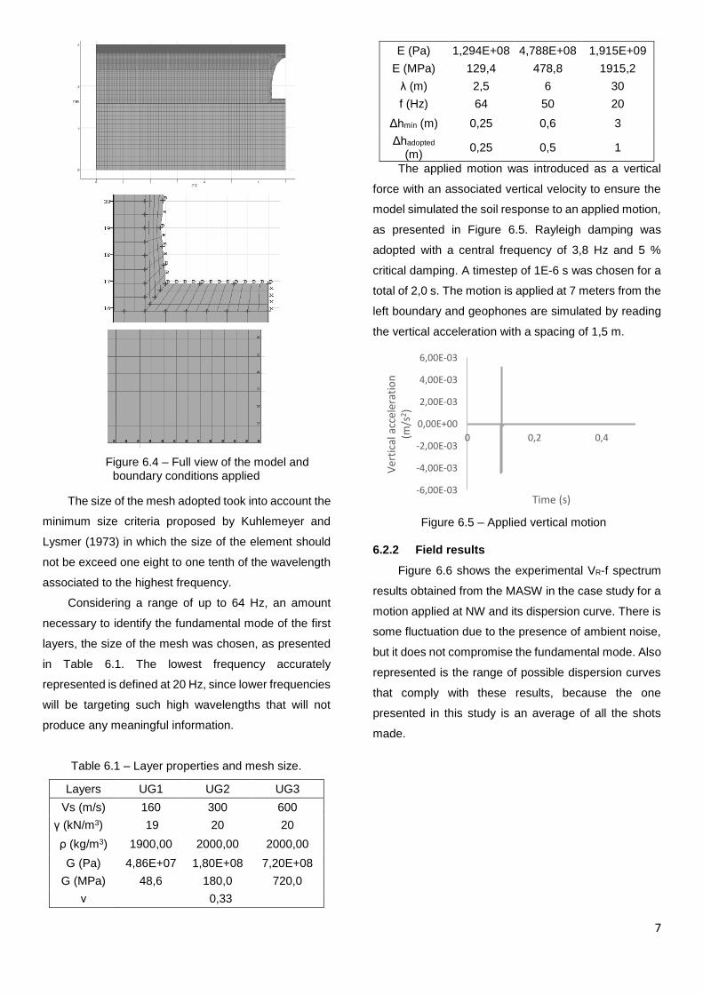
Figure 6.4 – Full view of the model and boundary conditions applied

The size of the mesh adopted took into account the

minimum size criteria proposed by Kuhlemeyer and

Lysmer (1973) in which the size of the element should

not be exceed one eight to one tenth of the wavelength

associated to the highest frequency.

Considering a range of up to 64 Hz, an amount

necessary to identify the fundamental mode of the first

layers, the size of the mesh was chosen, as presented

in Table 6.1. The lowest frequency accurately

represented is defined at 20 Hz, since lower frequencies

will be targeting such high wavelengths that will not

produce any meaningful information.

Table 6.1 – Layer properties and mesh size.

Layers UG1 UG2 UG3

Vs (m/s) 160 300 600

γ (kN/m3) 19 20 20

ρ (kg/m3) 1900,00 2000,00 2000,00

G (Pa) 4,86E+07 1,80E+08 7,20E+08

G (MPa) 48,6 180,0 720,0

ν 0,33

E (Pa) 1,294E+08 4,788E+08 1,915E+09

E (MPa) 129,4 478,8 1915,2

λ (m) 2,5 6 30

f (Hz) 64 50 20

Δhmín (m) 0,25 0,6 3

Δhadopted (m)

0,25 0,5 1

The applied motion was introduced as a vertical

force with an associated vertical velocity to ensure the

model simulated the soil response to an applied motion,

as presented in Figure 6.5. Rayleigh damping was

adopted with a central frequency of 3,8 Hz and 5 %

critical damping. A timestep of 1E-6 s was chosen for a

total of 2,0 s. The motion is applied at 7 meters from the

left boundary and geophones are simulated by reading

the vertical acceleration with a spacing of 1,5 m.

Figure 6.5 – Applied vertical motion

6.2.2 Field results

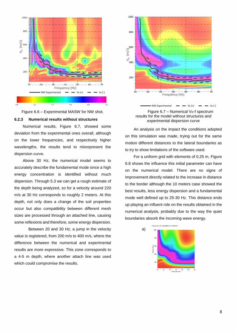
Figure 6.6 shows the experimental VR-f spectrum

results obtained from the MASW in the case study for a

motion applied at NW and its dispersion curve. There is

some fluctuation due to the presence of ambient noise,

but it does not compromise the fundamental mode. Also

represented is the range of possible dispersion curves

that comply with these results, because the one

presented in this study is an average of all the shots

made.

-6,00E-03

-4,00E-03

-2,00E-03

0,00E+00

2,00E-03

4,00E-03

6,00E-03

0 0,2 0,4

Ver

tica

l acc

eler

atio

n

(m/s

2 )

Time (s)

8

Figure 6.6 – Experimental MASW for NW shot.

6.2.3 Numerical results without structures

Numerical results, Figure 6.7, showed some

deviation from the experimental ones overall, although

on the lower frequencies, and respectively higher

wavelengths, the results tend to misrepresent the

dispersion curve.

Above 30 Hz, the numerical model seems to

accurately describe the fundamental mode since a high

energy concentration is identified without much

dispersion. Through 5.3 we can get a rough estimate of

the depth being analyzed, so for a velocity around 220

m/s at 30 Hz corresponds to roughly 2 meters. At this

depth, not only does a change of the soil properties

occur but also compatibility between different mesh

sizes are processed through an attached line, causing

some reflexions and therefore, some energy dispersion.

Between 20 and 30 Hz, a jump in the velocity

value is registered, from 200 m/s to 400 m/s, where the

difference between the numerical and experimental

results are more expressive. This zone corresponds to

a 4-5 m depth, where another attach line was used

which could compromise the results.

Figure 6.7 – Numerical VR-f spectrum results for the model without structures and

experimental dispersion curve

An analysis on the impact the conditions adopted

on this simulation was made, trying out for the same

motion different distances to the lateral boundaries as

to try to show limitations of the software used.

For a uniform grid with elements of 0,25 m, Figure

6.8 shows the influence this initial parameter can have

on the numerical model. There are no signs of

improvement directly related to the increase in distance

to the border although the 10 meters case showed the

best results, less energy dispersion and a fundamental

mode well defined up to 25-30 Hz. This distance ends

up playing an influent role on the results obtained in the

numerical analysis, probably due to the way the quiet

boundaries absorb the incoming wave energy.

VR

(m/s

)

Frequency (Hz)NW Experimental Vs (+) Vs (-)

VR

(m/s

)

Frequêncy (Hz)

NW Experimental Vs (+) Vs (-)

a)

9

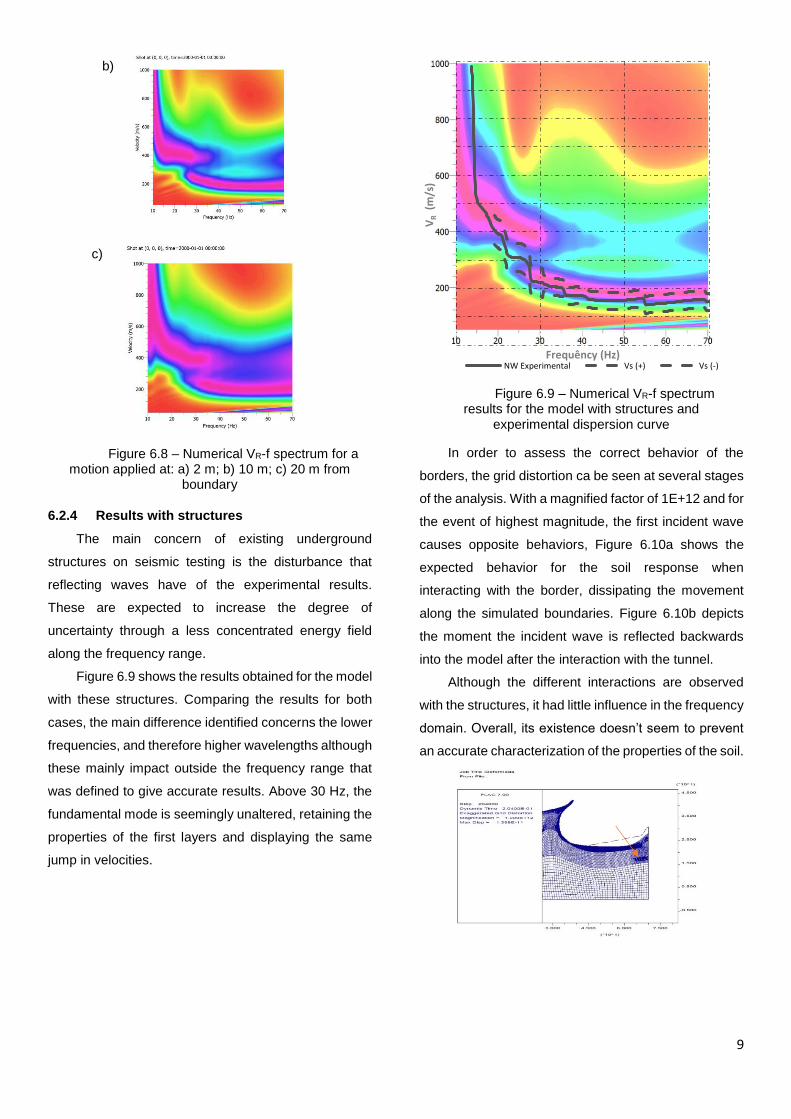
Figure 6.8 – Numerical VR-f spectrum for a motion applied at: a) 2 m; b) 10 m; c) 20 m from

boundary

6.2.4 Results with structures

The main concern of existing underground

structures on seismic testing is the disturbance that

reflecting waves have of the experimental results.

These are expected to increase the degree of

uncertainty through a less concentrated energy field

along the frequency range.

Figure 6.9 shows the results obtained for the model

with these structures. Comparing the results for both

cases, the main difference identified concerns the lower

frequencies, and therefore higher wavelengths although

these mainly impact outside the frequency range that

was defined to give accurate results. Above 30 Hz, the

fundamental mode is seemingly unaltered, retaining the

properties of the first layers and displaying the same

jump in velocities.

Figure 6.9 – Numerical VR-f spectrum results for the model with structures and

experimental dispersion curve

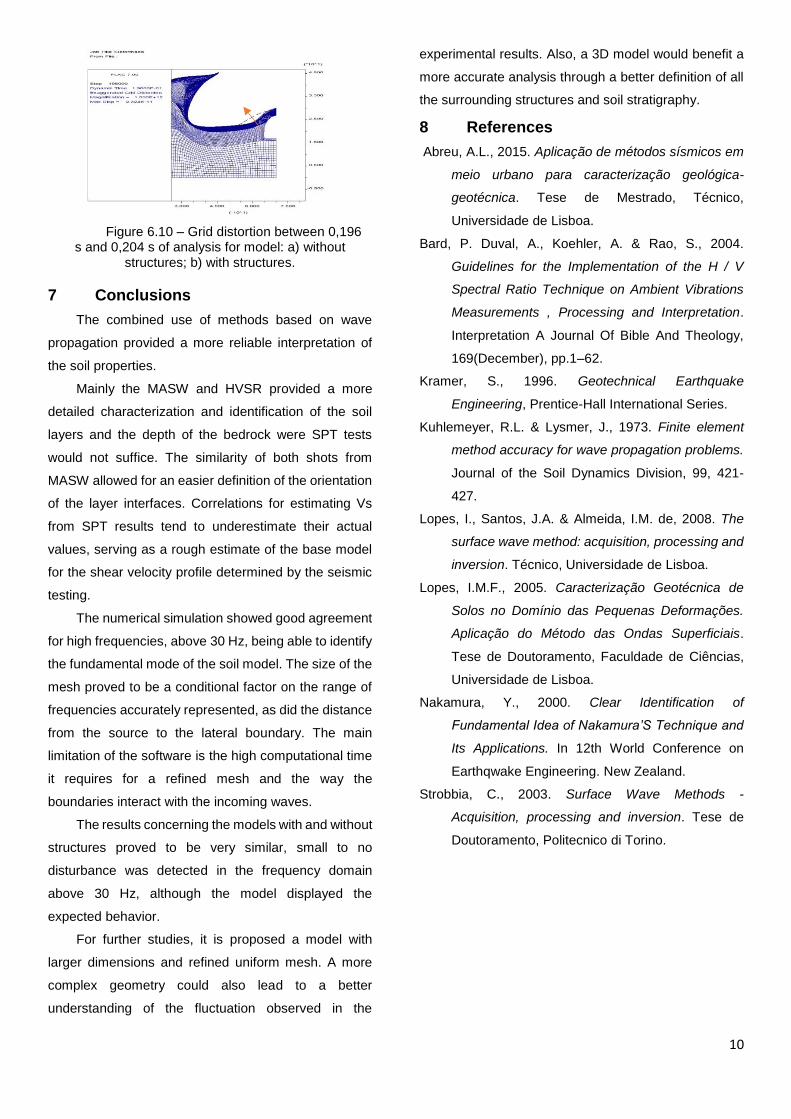
In order to assess the correct behavior of the

borders, the grid distortion ca be seen at several stages

of the analysis. With a magnified factor of 1E+12 and for

the event of highest magnitude, the first incident wave

causes opposite behaviors, Figure 6.10a shows the

expected behavior for the soil response when

interacting with the border, dissipating the movement

along the simulated boundaries. Figure 6.10b depicts

the moment the incident wave is reflected backwards

into the model after the interaction with the tunnel.

Although the different interactions are observed

with the structures, it had little influence in the frequency

domain. Overall, its existence doesn’t seem to prevent

an accurate characterization of the properties of the soil.

VR

(m/s

)

Frequêncy (Hz)NW Experimental Vs (+) Vs (-)

b)

c)

10

Figure 6.10 – Grid distortion between 0,196 s and 0,204 s of analysis for model: a) without

structures; b) with structures.

7 Conclusions

The combined use of methods based on wave

propagation provided a more reliable interpretation of

the soil properties.

Mainly the MASW and HVSR provided a more

detailed characterization and identification of the soil

layers and the depth of the bedrock were SPT tests

would not suffice. The similarity of both shots from

MASW allowed for an easier definition of the orientation

of the layer interfaces. Correlations for estimating Vs

from SPT results tend to underestimate their actual

values, serving as a rough estimate of the base model

for the shear velocity profile determined by the seismic

testing.

The numerical simulation showed good agreement

for high frequencies, above 30 Hz, being able to identify

the fundamental mode of the soil model. The size of the

mesh proved to be a conditional factor on the range of

frequencies accurately represented, as did the distance

from the source to the lateral boundary. The main

limitation of the software is the high computational time

it requires for a refined mesh and the way the

boundaries interact with the incoming waves.

The results concerning the models with and without

structures proved to be very similar, small to no

disturbance was detected in the frequency domain

above 30 Hz, although the model displayed the

expected behavior.

For further studies, it is proposed a model with

larger dimensions and refined uniform mesh. A more

complex geometry could also lead to a better

understanding of the fluctuation observed in the

experimental results. Also, a 3D model would benefit a

more accurate analysis through a better definition of all

the surrounding structures and soil stratigraphy.

8 References

Abreu, A.L., 2015. Aplicação de métodos sísmicos em

meio urbano para caracterização geológica-

geotécnica. Tese de Mestrado, Técnico,

Universidade de Lisboa.

Bard, P. Duval, A., Koehler, A. & Rao, S., 2004.

Guidelines for the Implementation of the H / V

Spectral Ratio Technique on Ambient Vibrations

Measurements , Processing and Interpretation.

Interpretation A Journal Of Bible And Theology,

169(December), pp.1–62.

Kramer, S., 1996. Geotechnical Earthquake

Engineering, Prentice-Hall International Series.

Kuhlemeyer, R.L. & Lysmer, J., 1973. Finite element

method accuracy for wave propagation problems.

Journal of the Soil Dynamics Division, 99, 421-

427.

Lopes, I., Santos, J.A. & Almeida, I.M. de, 2008. The

surface wave method: acquisition, processing and

inversion. Técnico, Universidade de Lisboa.

Lopes, I.M.F., 2005. Caracterização Geotécnica de

Solos no Domínio das Pequenas Deformações.

Aplicação do Método das Ondas Superficiais.

Tese de Doutoramento, Faculdade de Ciências,

Universidade de Lisboa.

Nakamura, Y., 2000. Clear Identification of

Fundamental Idea of Nakamura’S Technique and

Its Applications. In 12th World Conference on

Earthqwake Engineering. New Zealand.

Strobbia, C., 2003. Surface Wave Methods -

Acquisition, processing and inversion. Tese de

Doutoramento, Politecnico di Torino.