Ground-based retrieval of continental and marine warm ... · Indeed, the albedo controls the amount of reﬂected and ab- sorbed solar radiation and is then responsible for the mech-

Atmos. Meas. Tech., 4, 2749–2765, 2011www.atmos-meas-tech.net/4/2749/2011/doi:10.5194/amt-4-2749-2011© Author(s) 2011. CC Attribution 3.0 License.

AtmosphericMeasurement

Techniques

Ground-based retrieval of continental and marine warmcloud microphysics

G. Martucci and C. D. O’Dowd

School of Physics & Centre for Climate and Air Pollution Studies, Ryan Institute, National University of Ireland Galway,University Road, Galway, Ireland

Received: 7 June 2011 – Published in Atmos. Meas. Tech. Discuss.: 29 July 2011Revised: 6 December 2011 – Accepted: 7 December 2011 – Published: 15 December 2011

Abstract. A technique for retrieving warm cloud micro-physics using synergistic ground based remote sensing in-struments is presented. The SYRSOC (SYnergistic RemoteSensing Of Cloud) technique utilises a Ka-band Dopplercloud RADAR, a LIDAR (or ceilometer) and a multichan-nel microwave radiometer. SYRSOC retrieves the main mi-crophysical parameters such as cloud droplet number con-centration (CDNC), droplets effective radius (reff), cloud liq-uid water content (LWC), and the departure from adiabaticconditions within the cloud. Two retrievals are presentedfor continental and marine stratocumulus advected over theMace Head Atmospheric Research Station. Whilst the con-tinental case exhibited high CDCN (N = 382 cm−3; 10th-to-90th percentile [9.4–842.4] cm−3) and small mean effectiveradius (reff = 4.3; 10th-to-90th percentile [2.9–6.5] µm), themarine case showed low CDNC and large mean effectiveradius (N = 25 cm−3, 10th-to-90th percentile [1.5–69] cm−3;reff = 28.4 µm, 10th-to-90th percentile [11.2–42.7] µm) as ex-pected since continental air at this location is typically morepolluted than marine air. The mean LWC was compa-rable for the two cases (continental: 0.19 g m−3; marine:0.16 g m−3) but the 10th–90th percentile range was widerin marine air (continental: 0.11–0.22 g m−3; marine: 0.01–0.38 g m−3). The calculated algorithm uncertainty for thecontinental and marine case for each variable was, respec-tively, σN = 161.58 cm−3 and 12.2 cm−3, σreff = 0.86 µm and5.6 µm, σLWC = 0.03 g m−3 and 0.04 g m−3. The retrievedCDNC are compared to the cloud condensation nuclei con-centrations and the best agreement is achieved for a supersat-uration of 0.1 % in the continental case and between 0.1 %–0.75 % for the marine stratocumulus. The retrievedreff at thetop of the clouds are compared to the MODIS satellitereff:7 µm (MODIS) vs. 6.2 µm (SYRSOC) and 16.3 µm (MODIS)

Correspondence to:G. Martucci([email protected])

vs. 17 µm (SYRSOC) for continental and marine cases, re-spectively. The combined analysis of the CDNC and thereff, for the marine case shows that the drizzle modifies thedroplet size distribution andreff especially if compared torMODeff . The study of the cloud subadiabaticity and the LWC

shows the general sub-adiabatic character of both clouds withmore pronounced departure from adiabatic conditions in thecontinental case than in the marine.

1 Introduction

At the global scale clouds increase the reflection of incom-ing solar radiation from 15 % to 30 % with an overall forcingof about−44 W m−2. On the other hand, the reduced cloudthermal emission below clear-sky values enhances the cloudgreenhouse effect by about 31 W m−2 thus determining a netcooling effect of about 13 W m−2 (Ramanathan et al., 1989).The determination of the global cloud radiative forcing in-tended as the difference between the radiation budget com-ponents for cloudy conditions and clear-sky conditions is achallenging task which remains affected by a large uncer-tainty. The increase in global surface temperature of 0.6◦Cthat occurred in the last century corresponds to a change ofless than 1 % in the radiative energy balance between shortwave (SW) absorption and long wave (LW) emission fromthe Earth system (Kaufman et al., 2002). Despite the criticalrole of this energy mechanism, the balance between coolingand warming effect due to LW and SW net fluxes in cloudyregions remains one of the largest uncertainties when assess-ing the aerosol indirect effect. The fact that the greenhouseeffect due to cloud is orders of magnitude larger than the onethat would result from a hundredfold increase in CO2 mix-ing ratio as well as the fact that hydrometeors size and con-centration affect the cloud albedo are amongst the primarilyreasons why in the last 50 yr studying cloud microphysicsbecame paramount in order to understand climate changes.

Published by Copernicus Publications on behalf of the European Geosciences Union.

http://creativecommons.org/licenses/by/3.0/

2750 G. Martucci and C. D. O’Dowd: Retrieval of continental and marine warm cloud microphysics

Numerical models and observations can improve the knowl-edge of cloud microphysics both at global and regional scale;especially for the description of cloud formation, numericalsimulations at the regional and micro-scale (cloud-resolvedscale) permit to resolve with explicit integration schemes thecloud microphysical processes and to assess the aerosol in-direct effect. On the other hand, cloud and aerosols observa-tions can either be in situ or remotely sensed. In situ mea-surements represent typically a reference for the microphys-ical variables retrieved using ground-based remote sensinginstrumentation. The need of references becomes importantespecially when the microphysics is retrieved by the remotesensing instrumentation using integrated profiles and com-bined methods based on multiple sensors which introducea number of assumptions and large uncertainty. In situ ob-servations of cloud microphysical parameters are limited byboth the cost of performing the measurements and the avail-ability of the infrastructures. Ground-based remote sens-ing instrumentation can perform the retrieval of cloud mi-crophysics with cost-effective and continuous measurements.An efficient system of measurements must ensure the oper-ational retrieval of the main cloud microphysics parameterssuch as cloud droplet number concentration (CDNC), effec-tive radius (reff), liquid water content (LWC) and the albedo.Indeed, the albedo controls the amount of reflected and ab-sorbed solar radiation and is then responsible for the mech-anisms that initiates, maintains or inhibits the global cool-ing/warming. Alteration of the cloud albedo can occur byanthropogenic action: seeding experiments on marine stratusclouds by controlled release of aerosols (Durkee et al., 2000;Salter et al., 2008; Korhonen et al., 2010) demonstrate thecapability to modify the cloud albedo and to alter the cloudforcing at local scales. The cloud albedo is non-linearly re-lated to the cloud thickness, the LWC and the CDNC (Ack-erman et al., 2000; Seinfeld and Pandis, 2006). The level ofwater vapour supersaturation and the number of cloud con-densation nuclei (CCN) is also indirectly related to the cloudalbedo. In polluted air the number of CCN is supposed to in-crease rapidly leading to increased CDNC (Twomey, 1977),nevertheless the efficiency in activating CCN into CDNC de-pends on a number of factors including CCN size, chem-ical compositions and cloud dynamics (updraft and down-draft). There are instead no evidences of the impact of theentrainment-mixing on the activation process, although re-cent studies indicate homogeneous and inhomogeneous mix-ing as depleting mechanism for CDNC formation especiallyin warm cumuli (e.g. Morales et al., 2011). Several stud-ies in the last two decades showed different methodologiescapable to retrieve some microphysical parameters of liq-uid clouds by means of both independent and synergistic re-mote sensing instrumentation (Fox and Illingworth, 1997;Dong et al., 1997; Boers et al., 2000, 2006; Liljegren etal., 2001; Dong and Mace, 2003; Illingworth et al., 2007;Turner et al., 2007; Brandau et al., 2010). None of the citedmethodologies, however, provide the full set of microphys-

ical parameters (i.e. LWC, CDNC andreff). The state-of-the-art suggests that using synergistic information from pas-sive and active co-located remote sensors can provide suffi-cient cloud input parameters in order to retrieve cloud micro-physics with only a few assumptions. A synergistic suite ofremote sensors, namely a Ka-band Doppler cloud RADAR, aLIDAR-ceilometer and a multichannel microwave radiome-ter (MWR) installed at the GAW Atmospheric Station ofMace Head, Ireland, has been used to provide the input datato the SYRSOC (SYnergistic Remote Sensing Of Cloud)multi-module technique and to retrieve the three primary mi-crophysical parameters from liquid clouds. In addition to thethree main microphysical variables, SYRSOC can provide anumber of parameters describing the cloud droplet spectralproperties (relative dispersion) and cloud degree of subadi-abaticity. SYRSOC has been applied to two cases of warmstratocumulus clouds formed in continental and marine airto analyze how the different air masses and aerosol load in-fluence the cloud microphysics in determining CDNC,reff,LWC.

2 Site, instruments and cases selection

2.1 The site

Located on the west coast of Ireland, the Atmospheric Re-search Station at Mace Head (O’Connor et al., 2008), Carna,County Galway is unique in Europe in that its location offerswesterly exposure to the North Atlantic Ocean through theclean sector (190◦ N–300◦ N) and the opportunity to studyatmospheric composition under northern hemispheric back-ground conditions as well as European continental emissionswhen the winds favour transport from that region. The sitelocation (53◦ 20′ N and 9◦ 54′ W) is in the path of the mid-latitude cyclones which frequently traverse the North At-lantic. The instruments are located 300 m from the shore lineon a gently-sloping hill (4◦ incline).

2.2 The instruments

The CLOUDNET programme (Illingworth et al., 2007) hasaimed to provide near-continuous and near-real-time cloudproperties for both forecasting objectives and for advanc-ing of cloud-climate interactions. CLOUDNET promotes thesynergistic retrieval of cloud properties from a combinationof three instruments, namely a LIDAR (or a ceilometer), amicrowave humidity and temperature profiler and a K- toE-band cloud RADAR. The Atmospheric Station of MaceHead is part of the CLOUDNET programme since 2009;data from the Jenoptik CHM15K LIDAR ceilometer (Heeseet al., 2010; Martucci et al., 2010a) with 1064-nm wave-length and 15-km vertical range, the RPG-HATPRO (Crewelland Lohnert, 2003; Lohnert and Crewell, 2003; Lohnertet al., 2009) water vapour and oxygen multi-channel mi-crowave profiler and the MIRA36, 35 GHz Ka-band Doppler

Atmos. Meas. Tech., 4, 2749–2765, 2011 www.atmos-meas-tech.net/4/2749/2011/

G. Martucci and C. D. O’Dowd: Retrieval of continental and marine warm cloud microphysics 2751

cloud RADAR (Bauer-Pfundstein and Goersdorf, 2007; Mel-chionna et al., 2008) are used to retrieve the cloud micro-physics using SYRSOC and CLOUDNET.

2.3 Case selection

Cases are selected based on SYRSOC requirements, namely:(1) the studied cloud layer must be unique along the atmo-spheric column to ensure that the MWR-retrieved Liquid Wa-ter Path (LWP) belongs entirely to the studied cloud; (2) eventhough many clouds remain in the liquid state even when theyform well above the freezing height (Mason, 1971; Prup-pacher and Klett, 1978), the cloud layer should be locatedno more than 1000 m above the freezing level (∼ −6.5◦C instandard atmosphere) and preferably below it; (3) liquid pre-cipitation (LWP> 1000 g m−2), must be avoided for a cor-rect interpretation of the MWR data (Lohnert and Crewell,2003). If they occur, short rain events must be excluded forthe microphysical analysis. On the other hand, SYRSOC hasno limitations working in drizzle, which represents an advan-tage when dealing with stratocumulus forming in marine aircharacterized by large droplets growing fast by coalescenceand forming drizzle in most of the cases. Care must be usedwhen studying drizzle clouds in order to include the area withdrizzle within the actual cloud boundaries (see Sect. 3.1).In fact, the contribution of drizzle to the total liquid watermust be always considered in order to avoid errors in thefinal calculation of the cloud liquid water content. Basedon these requirements two cases of liquid clouds have beenselected for which the air masses originated from oppositesectors (Fig. 1): a continental drizzle-free stratiform cloud(28 May 2008) and a marine stratiform cloud with drizzle(10 December 2010). In-situ observations have been used tocompare the microphysics retrieved by SYRSOC with satel-lite reff and CCN sampled at the ground level.

3 Physics of SYRSOC

SYRSOC retrieves the microphysics of liquid clouds provid-ing CDNC, reff, relative dispersion and LWC. SYRSOC isa three-level algorithm (Fig. 2) acquiring off-line input datafrom the same suite of instrument as CLOUDNET. At eachlevel SYRSOC generates microphysical outputs which areused for the next computational level: the first level’s out-puts consist of the cloud boundaries, the LIDAR extinctionand the cloud subadiabaticity. The three outputs are calcu-lated using the reflectivity from the cloud RADAR, the atten-uated backscatter from the LIDAR and the temperature andthe integrated cloud liquid water from the MWR. The secondlevel’s output is the CDNC from the LIDAR extinction, thecloud depth and the cloud subadiabaticity. The third level’soutputs are thereff and the cloud LWC – both of which areretrieved using the CDNC, the level of cloud subadiabaticityand the droplet size distribution.

Fig. 1. 72-h backward trajectories (BT) calculated by NOAA HYS-PLIT model and based on GDAS Meteorological 1000-m BT on28 May 2008 (left) and 10 December 2010 (right).

3.1 Level 1: cloud boundaries determination

Detection of the cloud boundaries plays an important role inthe retrieval of cloud microphysics. Errors of few tens ofmeters in the detection of the cloud base can lead to errorsin the calculation of the CDNC. The extinction efficiencyQ,which will appear in the equation to calculate the CDNC,is sensitive to the cloud base height, its value quickly re-sponds to variations in the droplet size at the cloud base.Q

can be regarded as constant only when the mode of the size

www.atmos-meas-tech.net/4/2749/2011/ Atmos. Meas. Tech., 4, 2749–2765, 2011


Fig. 2. Outline of SYRSOC: three-level (blue-orange-red) retrievalscheme of cloud microphysical variables.

distribution exceeds 1 µm, i.e. the cloud base has to be care-fully detected in order not to include large aerosols below thereal cloud base. In drizzle-free conditions, the LIDAR (andceilometer) is the optimal remote sensor to detect the cloudbase, while the cloud RADAR is more reliable to providethe cloud top and the lower boundary of drizzle below theLIDAR-detected cloud base. The automated algorithm Tem-poral Height Tracking, THT, (Martucci et al., 2010a, b) hasbeen developed to detect the cloud base and top with highaccuracy. For this study the THT algorithm has been appliedto the LIDAR and RADAR profiles to determine the cloudboundaries.

3.2 Level 1: LIDAR extinction

The LIDAR extinction is expressed in terms of the extinc-tion coefficientσ (z) calculated by inverting the 1.064-µmLIDAR profiles (Klett, 1981; Ferguson and Stephens, 1983)in the lower part of the cloud where the LIDAR signal isnot completely attenuated, i.e. 100 up to 200 m above thecloud base (depending on the cloud optical thickness). LI-DAR calibration for molecular signal component is essentialto invert the LIDAR signal; it is performed between 4 and8 km above the LIDAR receiver preferably during night andfor integration time not shorter than 1 h. The LIDAR hasbeen calibrated in clear-sky condition by a multi-wavelengthsun photometer at the extrapolated wavelength of 1.064 µm,the LIDAR return has then been inverted between cloud baseand top assuming a LIDAR ratio ofS = 18.2± 1.8 sr (Pinnicket al., 1983). The assumed constant LIDAR ratio affects thederivation of the extinction by propagating through the stablesolution obtained by Klett (1981, Eq. 9). Because the numer-ical procedure used in this study to invert the LIDAR return(Ferguson and Stephens, 1983) is normalized byS, the mi-crophysical variables retrieved in the following sections are

physically independent ofS. However, as the LIDAR returnis mathematically divided byS, theS-error propagates to theextinction and to the other determinations and must be con-sidered when assessing the total uncertainty. In order to usethe entire extinction profile to retrieve the CDNC a curve fit isused to regress in least-squares sense the not-fully-attenuatedpart of theσ -profile and to extrapolate theσ -points (and thenthe CDNC) in the fully-attenuated region (see Sect. 3.4).

3.3 Level 1: subadiabaticity

In adiabatic conditions the LWC increases linearly from thebase to the top of the cloud. In order to provide a realis-tic representation of the liquid water profile through liquidclouds, a subadiabatic function is considered to describe theadiabatic departure at each heightz:

LWC(z) =4

3π ρw N(z)

⟨r3(z)

⟩= f (z) Aadz (1a)

The middle term in Eq. (1a) is proportional to the concen-tration of cloud dropletsN (N indicates CDNC in all equa-tions) and to the third moment of the droplets size distribu-tion (DSD). The term on the far-right introduces the suba-diabatic functionf (z) which depends on the heightz alongthe cloud layer and which modifies the vertical gradient ofthe adiabatic LWC,Aad, by providing the subadiabatic de-parture along the LWC profile. Different approaches to cal-culate the departure functionf (z) have been suggested inthe recent literature (Boers et al., 2000, 2006; Brandau et al.,2010): an expression forf (z) can be set up starting from thefar-right term in Eq. (1a) in saturated irreversible pseudoadi-abatic conditions:

LWC(z) = D ·A(z)SAT z (1b)

Here, the termD is a correction factor related to the subadi-abaticity and whose meaning will become clear with Eq. (2).The termASAT is the vertical rate of change of condensablewater during a saturated irreversible pseudoadiabatic process(Iribarne and Godson, 1973; Pruppacher and Klett, 1978)and depends on the temperature vertical profile through thecloud. Combining Eq. (1a) and (1b) we obtain the expressionof the departure functionf (z):

f (z) =D ·ASAT(z)

Aad(1c)

In contrast to the gradientAad, which has a constant valuewith height,ASAT slowly varies with height from cloud baseto cloud top and is a function of temperature and humid-ity. The change in condensable water in saturated condi-tions is then better represented byASAT =ASAT (T (z),P (z))

which can be calculated directly using the temperature fromthe MWR. Numerical derivation of the main parameters in-volved to calculate the dependence ofASAT on the pressure,P , and the saturation vapour pressure,es, can be obtained



from the parameterizations suggested by, amongst others,Richards (1971) and Rogers and Yau (1989).

In order to obtainf (z), the correction factorD must be de-termined by integration of Eq. (1b) over the cloud thickness.The measured LWP can then be used to obtain an expressionfor D:

LWP = D

zt∫zb

ASAT(z) zdz = D

[[ASAT(z)

∫zdz

]zt

zb

−

zt∫zb

(∫zdz

)A′

SAT(z)dz

(2)

SYRSOC inverts Eq. (2) with respect toD between the cloudbase (zb) and the cloud top (zt) at each time step.D accountsfor the departure of the calculated LWP (right-hand side ofEq. 2) from the measured LWP (left-hand side of Eq. 2). ThetermD is then a correction factor and accounts for the over-estimation (D < 1) or underestimation (D > 1) of the inte-grated termASAT · z with respect to the instrumental LWP.

3.4 Level 2: CDNC

The first microphysical variable retrieved by SYRSOC is theCDNC. The retrieval technique is based on the inherent linkbetween the CDNC, the LIDAR extinction,σ , and the LWCoutlined by Boers and colleagues in 1994, 2000 and 2006.We do not repeat here their calculations but only show theresult of their analysis assuming the DSD to be adequatelydescribed by a Gamma distribution. Then the number ofdropletsN at time t and heightz above the cloud base (zb)

can be written as

N(z) =

σ(z)

π1/3Qk2

(43ρw

)−2/3

f (z)2/3A

2/3ad (z−zb)

2/3

3

(3)

Here,ρw is the density of liquid water;σ is the extinctioncoefficient;Q is the extinction efficiency, which, in Mie ap-proximation for Gamma-type water DSD and for a LIDARwavelength of 1.06 µm, can be assumed constant,Q ≈ 2(Pinnick et al., 1983). The coefficientk2 is function of thesize parameterα of the Gamma distribution which describesthe droplet spectrum. It is convenient to adopt the alreadyknown and extensively used Gamma distribution (Boers andMitchell, 1994) to describe the size droplet spectrum forcases of liquid water clouds:

n (r, z) = a(z)r (z)α exp(−b(z)r (z)) (4)

where n is the droplet concentration density,r is the ra-dius of the droplets,b(z) is called rate parameter anda(z)

is a function of the rate parameter and the Gamma function(0(α)). The values ofα depend on the air mass in which thecloud forms and can be parameterized byα = 3 andα = 7 in

Fig. 3. Black solid: log-normal ideal extinction profile through thecloud layer; red crosses: lidar-retrievedσ -points; green dashed: notfully attenuated extinction profile; blue crosses: power-law extrap-olatedσ -points; black dashed: cloud top and base levels.

marine and continental air, respectively (Miles et al., 2000;Goncalves et al., 2008). Depending on the vertical resolu-tion of the extinction profile a limited number ofσ -points(normally 10–15 points with 15-m resolution) can be used toregress in a least-squares sense Eq. (3) to each extinction pro-file with N as a free parameter. The model used to fit Eq. (3)is a power-law of typey =C xb where the independent vari-ablex is the relative height above the cloud base multipliedby f (z) while N is kept constant and embedded into the con-stantC. Figure 3 shows a hypothetical case of cloud layerextending∼300 m above the cloud base. Four representa-tions of extinction profiles are pictured: a LIDAR-retrievedσ -profile in the not-fully-attenuated region (red crosses), thetheoretical LIDAR profile through the cloud layer (blacksolid), the not-attenuated extinction profile through the entirecloud layer (green dashed) as it could be retrieved by mea-surements made by particulate spectrometers carried aloft bytethered balloons (e.g. Lindberg et al., 1984) and the extrap-olatedσ -points as a result of they =C xb curve-fit (bluescrosses). The error related to the curve-fit to retrieveN rep-resents a major source of uncertainty, i.e. the extrapolatedσ -points can deviate from the not-attenuated extinction profilethrough the cloud (difference between the green curve andblue crosses in Fig. 3). Differences of both signs can lead toeither underestimated or overestimated values ofN produc-ing an uncertainty which propagates to the other microphys-ical variables (see Sect. 5). Once calculated, the CDNC isassumed to remain constant with height in the region of fullattenuation (using the mean value of blue crosses in Fig. 3).



3.5 Level 3:reff

The second microphysical variable calculated by SYRSOCis the reff, defined as the ratio of the third to the secondmoment of the DSD (Frisch et al., 1998, 2000). Fox andIllingworth (1997) found an almost one-to-one relation be-tween the RADAR reflectivity factor andreff. Based on thisrelation, reff can be expressed as the sixth root of the ratiobetween the detected RADAR reflectivity and the retrievedCDNC. Following Brandau’s calculations (2010)reff can bewritten as:

reff(z) =

⟨r(z)3

⟩⟨r(z)2

⟩ = k−12 f (z)

1/3⟨r(z)3

⟩1/3,

k2 =α

13 (α+1)

13

(α+2)23

(5)

Here, the termk2 is the same as in Eq. (3) and expressesthe constant relation between the second and the third mo-ment of the DSD. In case of Rayleigh approximation, therelation between〈r(z)6

〉 and the RADAR reflectivity factorZ [mm6 m−3] is:

〈r(z)6〉 =

Z(z)

64N(z)(6)

Using the relation between the third and the sixth moment ofthe DSD (Atlas, 1954; Frisch et al., 1998):

⟨r(z)3

⟩=

[ ⟨r(z)6

⟩k6f (z)2

]1/2, k6 =

(α+3)(α+4)(α+5)

α(α+1)(α+2)(7)

The coefficientk6 depends also on the shape parameterα

and expresses the constant relation between the sixth and thethird moment of the DSD.

Then, using Eqs. (5) and (6) and by combining withEq. (4),reff can be written as:

reff(z) = k−12 k

−16

6

(Z(z)

64N(z)

)1/6(8)

3.6 Level 3: LWC

The third microphysical variable calculated by SYRSOC isthe LWC which can be retrieved, as shown in Eq. (1a), as afunction of the third moment of the DSD and the retrievedCDNC. In the approximation of particles larger than the (LI-DAR) wavelength, the extinction can be related to the secondmoment of the DSD by (Boers and Mitchell, 1994):

σ(z) = 2π N(z)⟨r(z)2

⟩(9)

By combination of Eqs. (1a), (7) and (8) the LWC [g m−3]can be expressed in the form:

LWC(z) =1

3ρw N(z)−

16 k−1

2 k−

16

6 Z(z)16 σ(z) (10)

4 Results

All microphysical variables are calculated by SYRSOC andshown in two-panel figures for the continental and the ma-rine cases in the following sub-sections. A table at the endof Sect. 5 summarizes the comparison of the retrieved micro-physics with the related uncertainty for the two cases.

4.1 Subadiabatic functionf (z)

Subadiabatic conditions are mainly determined by entrain-ment of dry air at the top of the cloud and by mixing of di-luted and undiluted air at the cloud base due to updrafts anddowndrafts and to precipitation processes. The entrainmentat the cloud top enhances the droplets evaporation thus de-creasing their average radius; the CDNC at the cloud top canalso be depleted by the entrainment. By solving Eqs. (1–2)the subadiabatic functionf (z) can be determined and dis-played as in Fig. 4 for the case study 28 May 2008 (top panel)and the case 10 December 2010 (bottom panel). For the con-tinental case, the layer-averaged departure functionf (at thebottom of each panel) shows little variations throughout theduration of the Sc with overall values remaining slightly be-low 0.1. In the vertical direction,f (z) decreases with heightthrough the cloud asASAT becomes smaller compared toAad.During the first part of the Sc (21:30–22:30 UTC)f (z) isin the range 0.05–0.08 (f = 0.063); correspondingly to theincreased cloud thickness during 22:30–24:00 UTCf (z) in-creases showing values between 0.06 and 0.13 (f = 0.085).

The bottom panel shows the values off (z) for the ma-rine case: the Sc can be divided into three parts, from 11:00to 12:45 UTC, from 12:45 to 13:45 UTC and from 13:45 to16:00 UTC. The three intervals correspond to the periodsover which the cloud is more homogeneous. The overallvalue off (z) during the entire event is higher than in the con-tinental case, mainly due to the increased cloud thickness andthe reduced entrainment in the inner part of the cloud. Dur-ing the first and third partsf (z) ranges between 0.1 and 0.4(f = 0.24) and 0.1 and 0.3 (f = 0.2), respectively. During thecentral part (f = 0.09) the cloud most likely undergoes signif-icant entrainment and mixing with free-tropospheric air lead-ing to more subadiabatic conditions compared to the othercloud parts. BothAad andASAT are higher compared to thecontinental case showing that the rate of growth of the adia-batic LWC through the cloud is larger in marine than in con-tinental air. The relative and absolute humidity retrieved bythe MWR showed for both cases that the entrainment can re-duce the level of supersaturation and initiate the evaporationof cloud droplets while decreasing the amount of liquid waterespecially at the cloud top.



Fig. 4. Continental (top) and marine (bottom) case: subadiabatic function,f (z). Black solid lines at the bottom of top and bottom panels(right-hand y-axis) are the layer-averaged and 7.5-min averagedf (z).

4.2 CDNC

The results shown in Fig. 5 are obtained using Eq. (3). Con-tinental case: the mean CDNC is 382 cm−3, the medianis 180 cm−3 and the 10th to 90th-percentile range is 9.4–842.2 cm−3. The layer-averaged CDNC (black-solid line)has values mainly between 0 and 800 droplets cm−3 withpeaks at 1200 cm−3. The layer- and 7.5-min averaged CDNC(red-dashed line) remains around 500 droplets cm−3 duringthe period when the cloud is thicker (22:45–23:45 UTC). Incontinental Sc clouds the mean CDNC normally ranges be-tween 300 and 400 cm−3 (Miles et al., 2000) leading to smallreff and brighter clouds. The RADAR reflectivityZ dependson the sixth moment of the droplet size distribution, caus-ing continental clouds with high CDNC and smallreff to beassociated with smallZ-values. This is confirmed by thelow mean reflectivity factorZ =−44 dBZ and the low meanLWP = 40 g m−2. Drizzle is not present during the period ofobservation indicating that the coalescence process throughthe cloud layer is not as efficient as to generate droplets largeenough to fall out of the cloud. The layer-averaged CDNCshow significant variability at the temporal resolution of 0.5-min while almost all variability disappears reducing the tem-poral resolution to 7.5 min. The different temporal resolutionallows to study the effect of averaging on the indirectly re-

trieved cloud dynamics. The updraft and downdraft velocitycan be derived by the cloud RADAR Doppler velocity thatfor the continental and the marine cases is on the order of|0.5| m s−1 and∼ |1| m s−1, respectively. Because the meancloud depth where the cloud is thicker is∼0.5 km and∼1 kmfor the continental and marine clouds, this leads to∼15 minfor both cases to have the full ascent/descent of an air parcelthrough the cloud depth. The 7.5-min temporal resolution al-lows then to observe (where the process can be detected) thecloud dynamics while reducing significantly the noise. Theeffect of averaging will become even clearer when the re-trieved CDNC will be compared to the measured CCN at 10-min resolution (Sect. 4.2.1). The number of droplets remainssubstantially constant through the central and upper part ofthe layer with a net increase of CDNC occurring only in thebottom part of the cloud and leading to an average total ver-tical variability of about 10 % (CDNC variability only cor-responds to the not-fully-attenuated region, i.e. red crossesin Fig. 3). Conversely, the temporal variability of CDNC issignificant (10th to 90th-percentile range of variability cor-responds to the 218 % of the mean value) and is partiallyrelated to the updraft and downdraft cycle within the cloud.

Marine case: Fig. 5b shows the clean marine stratocu-mulus with mean CDNC as low as 25 cm−3, the me-dian is 10.5 cm−3 and the 10th to 90th-percentile range is



Fig. 5. Continental (top) and marine (bottom) case: time-height cross section of the CDNC [cm−3]. Layer-averaged black and red curves ateach panel’s bottom (right y-scale in [cm−3]) have 0.5-min and 7.5-min temporal resolution, respectively.

1.5–69 cm−3. The increased (compared to the continental)cloud vertical extent which includes the area with the driz-zle leads to the mean cloud thickness of 687 m (246 m forthe polluted). The lowest part of the cloud is the area whereonly the drizzle drops with very few counts (∼1 cm−3) arepresent; the depletion of CDNC in correspondence to thedrizzle affects the vertical variability which is as high as88 % (but it drops to 8 % if the drizzle region is not consid-ered). The temporal variability is as well considerably highand higher than the continental case, (10th to 90th-percentilerange of variability corresponds to the 270 % of the meanvalue). The small number of droplets combined with thepresence of drizzle is in agreement with the efficient pro-duction of large droplets, also supported by the high meanreflectivity factorZ =−8 dBZ.

4.2.1 CDNC-CCN

For boundary-layer clouds like the presented continental andmarine cases it is possible to perform an evaluation of theretrieved CDNC by comparing with in-situ measured CCN,notwithstanding the fact that such evaluation is difficult inits own right. In fact, with no in-situ CDNC available, wecompared the SYRSOC-retrieved CDNC with the surface-measured CCN (NCCN). The comparison has been per-

formed based on the fact that the boundary layer was well-mixed and that the surface CCN should reproduce well theCCN concentrations at cloud base (O’Dowd et al., 1992,1999). The CDNC-NCCN comparison provides a qualita-tive estimation of the supersaturation (ss) achieved within thecloud. Each ss scan lasts 5 min and, depending on the case,the selected ss values ranged from 0.1–0.25–0.5–0.75–1 %.The outcome of the comparison is shown at 10-min of tem-poral resolution in Fig. 6 for the continental (left) and themarine (right) case: for both cases the CDNC closely matchtheNCCN at one or more ss values. Whilst for the continen-tal case the comparison clearly suggests that the level of sswithin the cloud does not exceed 0.1 % (i.e. 100.1 %), forthe marine case the CDNC curve lays between 0.1 % and0.75 % ss. The average ss within the continental cloud islower than the marine cloud suggesting a larger entrainmentfor the continental case. The lower ss for the continental casecan be explained partly by the cloud dynamics and partly bythe largerNCCN that tends to reduce peak ss (Hudson et al.,2010). It should also be noticed that for the marine cloud thederived ss is influenced by droplet removal due to entrain-ment and coalescence scavenging (drizzle formation). As aconsequence, the derived ss is an underestimate of the peakss reached during the activation phase. The 10-min reso-lution suggests different reasons for the CDNC variability



Fig. 6. Continental (left) and marine (right) case: comparison be-tween CDNC and CCN at supersaturation levels of 0.1 %–0.25 %–0.5 %–0.75 %. Temporal resolution is 10 min.

during the retrieval time in the two cases: while for the con-tinental case the 0.1 % ssNCCN is very stable, for the marinecase theNCCN at all ss-levels vary up to 300 % of their meanvalue. The CDNC follow theNCCN changes in the marinecase which suggests that the variability does not come fromthe cloud dynamics. On the other hand, for the continen-tal case, the CDNC show∼30-min timescale variability thatcould depend primarily on the updraft and downdraft cycle.

4.3 reff

Thereff values shown in Fig. 7 are retrieved using Eq. (7), inthe right-hand frames are shown examples of near-adiabaticand sub-adiabaticreff mean profiles corresponding to relativemaximum and minimum off (z), respectively. Continentalcase: sincereff depends directly on the RADAR reflectivity

factor, in drizzle-free conditions the lowest part of the cloudwhere the smallest droplets are confined is often not detectedby the cloud RADAR. This happens normally with dropletsreff smaller than 2 µm which are found at the cloud base.When, like for this case, the entrainment at the top of thecloud is significant the cloud droplets can partially evaporatedue to the lower relative humidity leading to smaller droplets.For this reason in the top panel of Fig. 7 thereff data are miss-ing immediately below and above the cloud top and base, re-spectively. The meanreff is 4.3 µm, the median is 3.95 µmand the 10th to 90th-percentile range is 2.91–6.45 µm. Thesmall mean (and median) effective radius is in agreementwith the low value ofZ discussed in the previous section.Moreover, the low mean LWP (LWP = 40 g m−2) suggeststhat not too much water vapour was available for condensa-tion onto the CCN, thus limiting their condensational growthinto largereff. The nearly-adiabaticreff profile shows a con-stant increase in radius from cloud base to cloud top, on theother hand the sub-adiabaticreff profile has more irregularvertical trend with a peak at the cloud base probably due todrizzle onset.

Marine case: the meanreff value is 28.4 µm, the median is23.6 and the 10th to 90th-percentile range is 11.2–42.7 µm.The very large meanreff results from including the drizzlereff in the average, and it is then not representative of theCDNC-weightedreff distribution. The mean number of driz-zle drops is, as stated above,N = 1 cm−3 then a correct mea-sure of the modalreff must come from CDNC-weighted anal-ysis of the effective DSD. Differently from the continentalcase, both the near-adiabatic and subadiabatic profiles have avery large peak (reff > 40 µm) corresponding to fully devel-oped drizzle. Compared to the subadiabatic, with approxi-mately 19-µm profile through the cloud, the near-adiabaticprofile shows much larger radii through the actual cloud(40> reff > 80 µm). The trend decreases from base to topof the cloud suggesting that coalescence dominates thereffduring that time interval.

4.3.1 MODIS effective radius

A comparison between SYRSOC-retrieved and satellite-retrievedreff has been performed for the continental and ma-rine stratocumuli. L2reff products from TERRA and AQUAModerate-resolution Imaging Spectroradiometer (MODIS)satellites have been extracted for the overpasses containingthe Mace Head station (53.33◦ N, 9.9◦ W). For the continen-tal case (28 May 2008) no overpass was available duringthe retrieval period 21:30–24:00 UTC; the (temporally) clos-est overpass was then selected at 12:20 UTC when a similarcloud field was present over Mace Head. The 12:20 UTCTERRA-overpass can be used as qualitative indication ofthe reff a few hours later since the air mass did not changeand the number of CCN remained fairly constant duringthe period 12:00–24:00 UTC. Figure 8 shows the two over-passes for the continental (left) and marine (right) case with



Fig. 7. Continental (top) and marine (bottom) case: time-height cross section of the effective radiusreff [µm]. Layer-averaged black andred curves at each panel’s bottom (right y-scale in [µm]) have 0.5-min and 7.5-min temporal resolution, respectively. Profiles in highlightedframes show near-adiabatic (solid red) and sub-adiabatic (dashed blue)reff profiles corresponding to, respectively, maxima and minima ofthe departure functionf (z).

highlighted 0.6× 0.6-degrees box embedding the Mace Headgeographical position. The two box-averagedreff valuesare compared with the mean cloud topreff for the conti-nental and marine cases. The 14:00–14:30 UTC time in-terval has been selected to compare SYRSOC and MODISreff. In daytime, effective radius from MODIS is calculatedfrom the combination of reflectances in two channels in thevery-near infrared, and in the near-infrared. Therefore, theMODIS measurement ofreff comes from the cloud emittingregion in the very-near and near-infrared (Platnick, 2000).If it is assumed that the dominant region for emission inthis band is similar to the region where the cloud is opti-cally thick, then, for the downward observation, this wouldbe the top couple of hundred metres of a liquid layer. TheMODIS-retrievedreff would then be more representative ofthe cloud upper layer and should then be compared with theSYRSOC-retrieved meanreff from the upper 100-m cloudlayer. For the continental case, the satellite-retrievedreff was7 µm to be compared with the upper layer SYRSOC-retrievedreff which was 6.2 µm. The SYRSOC-retrievedreff resultsfrom an average over the period when the cloud was opti-cally thicker (22:40–24:00 UTC). For the marine case, the

satellite-retrievedreff was 16.2 µm and 17 µm was the upperlayer SYRSOC-retrievedreff during 14:00–14:30 UTC.

4.3.2 Effective DSD analysis

The vertical profiles ofreff show very low degree of variabil-ity in the drizzle region and higher within the cloud. Thereffvertical variability can be expressed as the ratio of the stan-dard deviation to the meanreff where the variability givesinformation on the droplet spectral dispersion. Both, theCDNC-weightedreff modal value and relative dispersion areshown in Fig. 9 for both the continental and the marine case.Figure 9 shows the relative dispersion index (Lu and Sein-feld, 2006; Lu et al., 2009), thereff Frequency Distribution(RFD) normalized by the total cloud CDNC and the relationbetween the available cloud water (in terms of LWP) and theactivated particles. The indexd is the ratio of the standard de-viation (droplet spectral width) to the meanreff of the cloudDSD:

d = σreff

/reff (11)



Fig. 8. MODIS-TERRA cloud effective radius from 12:20 UTCoverpass on 28 May 2008 (left) and MODIS-AQUA cloud effectiveradius from 14:20 UTC overpass on 10 December 2010 (right). Inenlarged frames are shown the 0.6× 0.6 deg box containing MaceHead Station (53.33◦ N, −9.9◦ E).

Continental case: the left panel shows the relative dis-persion indexd as function of the layer-averaged CDNC.The scatter diagram shows the relative dispersion decreas-ing with increasing CDNC, i.e. the spectral width of thedroplet distribution become narrower when the number ofparticles increases. The middle panel shows the RFD ver-sus thereff between 0 and 30 µm. The RFD represents theCDNC-weightedreff distribution and shows that the modalreff (rMOD

eff = 4.7 µm) is almost in a 1:1 relation withreff. Thenarrow RDF and the correspondence between modal andmeanreff is due to the drizzle-free conditions in which thecontinental Sc formed, more information will be added tothe interpretation of this result after the analysis of the ma-rine case. The right panel shows the Equivalent CDNC, i.e.

the ratio between the activated particles and the total amountof liquid water in the cloud (CDNC/LWP). The ratio providesinformation on the efficiency to generate the CDNC. Therelatively high mean Equivalent CDNC (9.94 cm−3 g−1 m2,dashed horizontal line) gives an alternative representation ofthe continental conditions in which the cloud formed.

Marine case: in contrast to the continental case, the rel-ative dispersiond does not show correlation with the aver-aged CDNC. In correspondence with the drizzle the relativedispersion is high suggesting a broad spectral width. Thedispersion remains uncorrelated with the CDNC also whenthe CDNC increases. A reason for that is the low CDNC inthe cloud, i.e. the relative dispersion normally starts decreas-ing for CDNC> 100 cm−3 (e.g. continental case), but for thestudied marine case the CDNC do not exceed the value of80 cm−3 unless by a negligible fraction of occurrences. Inthe middle panel it is shown a much broader RDF than thecontinental case with occurrences over the entire 0–30 µmspectrum and modalrMOD

eff = 12 µm. In contrast to the conti-nental case, thereff (28.4 µm) does not correspond torMOD

effbeing twice its value. The departure is due to the marginal(in terms of occurrences) contribution of drizzle to the cloudreff. The right panel shows the Equivalent CDNC which, es-pecially when compared with the continental case, well de-scribes the marine characteristic of the studied Sc with verylow equivalent CDNC (0.16 cm−3 g−1 m2).

4.4 LWC

The results shown in Fig. 10 are obtained using Eq. (9). Con-tinental case: the mean LWC is 0.19 g m−3, the median is0.15 g m−3 and the 10th to 90th-percentile range is 0.11–0.22 g m−3. In purely adiabatic conditions the LWC wouldincrease linearly with the slopeAad, leading to higher con-tent of liquid water at the cloud top than in subadiabatic con-ditions (slopeASAT). In agreement with the calculated valuesof f (z), the vertical LWC profiles are subadiabatic duringmost of the Sc with only short near-adiabatic periods. Toppanel of Fig. 10 shows in highlighted frames an example ofnear-adiabatic and sub-adiabatic LWC mean profiles corre-sponding to relative maximum and minimum off (z), re-spectively. Equation (9) expresses the LWC in terms of boththe LIDAR extinctionσ and the RADAR reflectivity factorZ, so that the LWC depends on the optical cloud propertiesat different wavelengths. The dependence on both Mie andRayleigh scattering ensures a correct representation of thecontribution from both small and large droplets to the LWC.

Marine case: the mean LWC is 0.16 g m−3, the medianis 0.13 g m−3 and the 10th to 90th-percentile range is 0.01–0.38 g m−3. Compared to the continental case the meanvalue is smaller due to the small contribution of drizzle tothe total amount of liquid water. Compared to the con-tinental case, the larger cloud depth over which the ris-ing air parcel can grow in liquid water determines a largerpeak LWC (0.37 g m−3 for the continental and 1.25 g m−3



Fig. 9. Continental (top) and marine (bottom) case: relative dispersion indexd (%, left); normalizedreff Frequency Distribution (RDF)versus dropletreff between 0 and 30 µm (middle); right panel: equivalent CDNC (cm−3 g−1 m2, right).

for the marine case). The larger degree of LWC vari-ability is then responsible for the larger standard deviation(σmarine/σcontinental= 400 %). Also the overall larger values off (z) suggests a more efficient LWC growth for the marinecase than for the continental. The LWC is indeed showingnear-adiabatic growth (bottom panel Fig. 10) and local peaksin correspondence to thef (z) local maxima (11:45–12:15and 14:10–14:30 UTC). Conversely, during the time intervalswhenf (z) shows a minimum the LWC peaks are located be-low the cloud top or even at mid-height between base andtop.

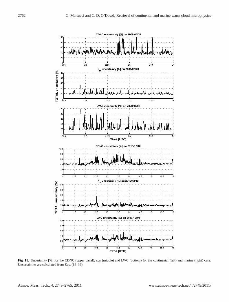
5 Error analysis and method sensitivity

An error analysis and method sensitivity study is needed inorder to asses SYRSOC. Three assumptions are made onthe parameters in Eq. (3): (i) the extinction efficiency co-efficient Q at the wavelength 1.064 µm is set to the con-stant valueQ = 2 (Bohren and Huffman, 1983); based onthe calculations of Nussenzveig and Wiscombe (1980) andPinnick and colleagues (1983), in the range of droplet radii1–15 µm, the error introduced assuming constantQ = 2, is1Q =−0.15 (6.8 %) at 1 µm and1Q = +0.106 (4.8 %) at15 µm. At larger radii the error rapidly drops below 1 %.(ii) The termk2 depends on the exponent of the size param-eter of the assumed Gamma distribution which describes the

DSD. The value ofα depends on the type of air mass and candouble from marine to continental air (Miles et al., 2000).Nonetheless, the method is sufficiently stable with respect tothe variations ofα: whenα is in the range from 2 to 50 therelative changes in the retrieved CDNC are between 0 and14 %. (iii) The correction termD in Eq. (2) depends on therate of change of condensable water during irreversible satu-rated pseudoadiabatic process (ASAT) which in turn, dependson the radiometric cloud base temperature that has an accu-racy of±0.7 K in the first 1000 m. The overall uncertainty onthe CDNC due toASAT can be regarded as systematic and itscontribution as large as 6 %. Assuming all the terms in (i)–(iii) as independent, the total contribution to the (maximum)uncertainty is the systematic error1Nsyst= 16.7 %.

The retrieval of the CDNC using Eq. (3) suffers the un-certainty introduced by the curve-fit regression of the extinc-tion (1σfit) in the region where the LIDAR signal is fullyattenuated and by the assumption of the constant LIDARratio, S. Both errors propagate also toreff and LWC de-terminations. The error introduced normalizing the LIDARsignal byS (1σS) propagates non-linearly first to the ex-tinction’s stable solution (Klett, 1981, Eq. 9) and then tothe other microphysical variables. The total uncertainty re-lated the calculation of the extinction can then be written as1σ =

√(1σfit)2 + (1σS)2. The error1σfit is determined by

the goodness-of-fit (GOF); the statistical parameters defin-ing the GOF are the degrees of freedom, the coefficient of



Fig. 10. Continental (top) and marine (bottom) case: time-height cross section of the liquid water content [g m−3]. Layer-averaged blackand red curves at each panel’s bottom (right y-scale in [g cm−3]) have 0.5-min and 7.5-min temporal resolution, respectively. Profiles inhighlighted frames show near-adiabatic (red) and sub-adiabatic (blue) LWC profiles corresponding to, respectively, maxima and minima ofthe departure functionf (z).

determination and the root mean square error (RMSE) of thefit, but only the RMSE is retained to determine1σfit .

The other source of uncertainty regards the departure func-tion f (z) calculated as the ratio of the product betweenASAT

and the correction termD to the adiabatic rateAad. The re-trieval of the termD depends on the total (integrated) contentof water through the cloud and on the cloud thickness. In-verting the integrated relation in Eq. (2) to obtainD it is pos-sible to shelve any dependence ofD on the vertical profileof the LWC excluding all a-priori assumption on the valueof LWC. Nevertheless, the termD depends on the MWR-retrieved LWP which suffers a maximum±15 g m−2 error.The error onD propagates then to the retrieval off (z) (1f )

through Eq. (1c) and finally toN and the other microphysicalvariables through Eqs. (3), (7) and (9). The total uncertaintyintroduced by the two sources of statistical (1σ and1f ) andsystematic (1Nsyst) error can be calculated by standard errorpropagation theory. Based on Eqs. (3), (10) and (12) the rela-tive uncertainties for CDNC,reff and LWC are, respectively:

1N =

[(3N

σ1σ

)2

+

(3N

f1f

)2

+(1Nsyst

)2

]1/2(12)

1reff =1

6

reff

N1N (13)

1LWC =

[(−

1

6

LWC

N1N

)2

+

(LWC

σ1σ

)2]1/2

(14)

The CDNC retrievals show the largest uncertainty for boththe continental and the marine case. Both1σ and1f areassumed to have zero-covariance matrix when they propa-gate to the other variables. Figure 11 shows the total uncer-tainty (in %) for the CDNC (upper panel),reff (middle panel)and the LWC (bottom panel) for the continental (left) and themarine (right) case, respectively.

For both the continental and marine case, the CDNC isaffected by the largest uncertainty with an average value of42 % (continental) and 49 % (marine). Thereff has aver-age uncertainty 20 % (continental) and 19.1 % (marine); theLWC uncertainty has values in between the two other re-trievals, 18.4 % (continental) and 25 % (marine). The meanvalue, the uncertainty and statistical variability of each mi-crophysical variable is summarized in Table 1 for the con-tinental and marine case. For each variable the table shows



Fig. 11. Uncertainty [%] for the CDNC (upper panel),reff (middle) and LWC (bottom) for the continental (left) and marine (right) case.Uncertainties are calculated from Eqs. (14–16).



Table 1. For each microphysical variable (1st column) the tableshows the mean valuex with the related total uncertainty1x (2ndand 4th column) and the 10th–90th percentile range of variabilityover the cloud lifetime (3rd and 5th column).

Microphysical Continental Continental Marine Marinevariable x ±1x 10th–90th x ±1x 10th–90th

percentile percentile

CDNC [cm−3] 382± 161.58 9.8–842.4 25± 12.2 1.5–69reff [µm] 4.3± 0.86 2.9–6.5 28.4± 5.6 11.2–42.7LWC [g m−3] 0.19± 0.03 0.11–0.22 0.16± 0.04 0.01–0.38

the mean valuex with the related uncertainty1x (2nd and4th column) and the variability in terms of the 10th–90th per-centile range (3rd and 5th column).

6 Conclusions

An assessment of the new technique SYRSOC (SYnergis-tic Remote Sensing Of Cloud) has been performed by deter-mining the microphysics of two liquid stratocumulus cloudswhich formed in continental and marine air masses. The con-tinental event occurred on the 28 May 2008 from 21:30 UTCto 24:00 UTC while the marine occurred on the 10 Decem-ber 2010 from 11:00 UTC to 16:00 UTC. The mean blackcarbon concentration (as a proxy for pollution) during thetwo events was 300 ng m−3 and 2.5 ng m−3 for the conti-nental and the marine event, respectively. The aim of thestudy is to provide the full cloud microphysics by apply-ing SYRSOC to the synergistic suite of three remote sen-sors, namely cloud RADAR, LIDAR and MWR installed atthe GAW Atmospheric Station of Mace Head, Ireland. Forgiven vertical and temporal resolutions SYRSOC retrievesthe three main microphysical variables, namely CDNC,reffand LWC at all heights above the cloud base and instantsin time. The retrieved CDNC have been compared to theconcentration of CCN sampled few meters above the groundlevel at different supersaturations. The comparison showedgood matching between the retrieved number of dropletsand the sampled CCN suggesting that the studied boundary-layer stratocumuli had ss≈ 0.1 % for the continental and0.1 %≤ ss≤ 0.75 % for the marine case. A combined anal-ysis of the CDNC and thereff showed that whilst in marineconditions the drizzle modified the retrieval of the mean ef-fective radius determining a large mean value (28.4 µm) morethan two times larger than the modereff (12 µm), in continen-tal condition the absence of drizzle led to almost 1:1 relationbetween mean and modereff (4.3 µm vs. 4.7 µm). Moreover,in continental conditions the spectral width of the effectiveDSD becomes narrower when the droplets concentration in-creases (dispersion index). On the contrary, the relation be-tween the relative dispersion and the CDNC does not showcorrelation for the marine case most likely because the very

low CDNC (N = 25 cm−3) where the relative dispersion nor-mally starts to decrease for CDNC> 100 cm−3. The RDFanalysis showed that the RDF is mono-modal in both caseswith narrow spectral width centred onrMOD

eff in the continen-tal case and broad spectral width in the marine case with anextended tail at the drizzle radii. The mode radiusrMOD

eff forthe two cases confirms the Twomey theory about the depen-dence of the DSD on the number of droplets in the cloud. Theretrievedreff at the top layer of the clouds have been com-pared with the MODIS satellitereff showing good matching:7 µm (MODIS) vs. 6.2 µm (SYRSOC) and 16.3 µm (MODIS)vs. 17 µm (SYRSOC) for continental and marine cases, re-spectively.

The study of the departure functionf (z) and the LWC pro-files shows a general subadiabatic character of both cloudswith more pronounced departure in the continental case dueto the shallower cloud depth and the significant mixing withdry tropospheric air.

Finally, an error analysis has been performed to as-sess the method accuracy. The CDNC retrieval suffersthe largest uncertainty compared toreff and LWC re-trievals. The error-corrected values of the retrieved mi-crophysical variables are for the continental and marinecase, respectively, 382± 161.58 cm−3 and 25± 12.2 cm−3

for the CDNC; 4.3± 0.86 µm and 28.4± 5.6 µm for reff;0.019± 0.035 g m−3 and 0.016± 0.042 g m−3. The retrievedmean values of the microphysical variables are in agreementwith the results shown by Miles et al. (2000) for continentaland marine stratocumulus clouds.

Acknowledgements.The authors would like to acknowledgeHerman W. J. Russchenberg and Christine Brandau from DelftUniversity of Technology (The Netherlands) for their precious sci-entific support as well as David Donovan and Rob Roebeling fromKNMI (The Netherlands) and Domenico Cimini from IMAA-CNR(Italy) for supplying satellite data and for the important support intheir interpretation. This study was supported by the 4th HigherEducation Authority Programme for Research in Third LevelInstitutions (HEA PRTLI4) and by EPA Ireland through the CCRPFellowship “Research Support for Mace Head”. This work wasalso conducted as part of COST Action ES0702 (EG-CLIMET).

Edited by: A. Kokhanovsky

References

Ackerman, A. S., Toon, O. B., Taylor, J. P., Johnson, D. W., Hobbs,P. V., Ferek, R. J.: Effects of Aerosols on Cloud Albedo: Evalu-ation of Twomey’s Parameterization of Cloud Susceptibility Us-ing Measurements of Ship Tracks, J. Atmos. Sci., 57, 2684–2695, 2000.

Albrecht, B. A., Fairall, C. W., Thomson, D. W., White, A. B.,Sauder, J. B., and Schubert, W. H.: Surface-based remote sensingof the observed and adiabatic liquid water content of stratocumu-lus, Geophys. Res. Lett., 17, 89–92, 1990.

Atlas, D.: The estimation of cloud parameters by radar, J. Meteorol.,11, 309–317, 1954.



Boers, R. and Mitchell, R. M.: Absorption feedback in stratocumu-lus clouds: Influence on cloud top albedo, Tellus, 46A, 229–241,1994.

Boers, R., Russchenberg, H., Erkelens, J., and Venema, V.:Ground-based remote sensing of stratocumulus properties duringCLARA, 1996, J. Appl. Meteorol., 39, 169–181, 2000.

Boers, R., Acarreta, J. R., and Gras, J. L.: Satellite Monitoringof the First Indirect Aerosol Effect: Retrieval of Droplet Con-centration of Water Clouds, J. Geophys. Res., 111, D22208,doi:10.1029/2005JD006838, 2006.

Bohren, C. F. and Huffman, D.: Absorption and scattering of lightby small particles, Wiley, New York, 530 pp., 1983.

Brandau, C. L., Russchenberg, H. W. J., and Knap, W. H.: Evalu-ation of ground-based remotely sensed liquid water cloud prop-erties using shortwave radiation measurements, Atmos. Res., 96,366-377,doi:10.1016/j.atmosres.2010.01.009, 2010.

Brenguier, J. L: Parameterization of the condensation process: Atheoretical approach, J. Atmos. Sci., 48, 264–282, 1991.

Chylek, P. and Ramaswamy, V.: Simple approximation for infraredemissivity of water clouds. J. Atmos. Sci., 39, 171–177, 1982.

Chylek, P.: Extinction and liquid water content of fogs and clouds,J. Atmos. Sci., 35, 296–300, 1978.

Crewell, S. and Lohnert, U.: Accuracy of cloud liquid water pathfrom ground-based microwave radiometry 2. Sensor accuracyand synergy, Radio Sci., 38, 8042,doi:10.1029/2002RS002634,2003.

Dong, X., Ackerman, T. P., Clothiaux, E. E., Pilewskie, P., andHan, Y.: Microphysical and radiative properties of stratiformclouds deduced from ground-based measurements, J. Geophys.Res., 102, 23829–23843, 1997.

Dong, X. and Mace, G. G.: Profiles of low-level stratus cloud mi-crophysics deduced from ground-based measurements, J. Atmos.Ocean. Tech., 20, 42–53, 2003.

Durkee, P. A., Noone, K. J., Ferek, R. J., Johnson, D. W., Tay-lor, J. P., Garrett, T. J., Hobbs, P. V., Hudson, J. G., Bretherton,C. S., Innis, G., Frick, G. M., Hoppel, W. A., O’Dowd, C. D.,Russell, L. M., Gasparovic, R., Nielsen, K. E., Tessmer, S. A.,Ostrom, E., Osborne, S. R., Flagan, R. C., Seinfeld, J. H., andRand, H.: The Impact of Ship-Produced Aerosols on the Mi-crostructure and Albedo of Warm Marine Stratocumulus Clouds.A Test of the MAST Hypothesis 1i and 1ii, J. Atmos. Sci, 57,2554–2569, 2000.

Ferguson, J. A. and Stephens, D. H.: Algorithm For Inverting LidarReturns, Appl. Optics, 22, 3673–3675, 1983.

Frisch, A. S., Feingold, G., Fairall, C. W., Uttal, T., and Snider, J.B.: On cloud RADAR and microwave radiometer measurementsof stratus cloud liquid water profiles, J. Geophys. Res., 103, 195–197, 1998.

Fox, N. I. and Illingworth, A. J.: The retrieval of stratocumuluscloud properties by ground-based cloud RADAR, J. Appl. Mete-orol., 36, 485–492, 1997.

Goncalves, F. L. T., Martins, J. A., and Silva Dias, M. A.: Shapeparameter analysis using cloud spectra and gamma functions inthe numerical modeling RAMS during LBA Project at Amazo-nian region, Brazil, Atmos. Res., 89, 1–11, ISSN 0169-8095,doi:10.1016/j.atmosres.2007.12.005, 2008.

Haeffelin, M., Angelini, F., Morille, Y., Martucci, G., O’Dowd, C.D., Xueref-Remy, I., Wastine, B., Frey, S., and Sauvage, L.:Evaluation of mixing depth retrievals from automatic profiling

lidars and ceilometers in view of future integrated networks inEurope, Bound.-Lay. Meteorol.,doi:10.1007/s10546-011-9643-z, 2011.

Hale, G. M. and Querry, M. R.: Optical Constants of Water in the200-nm to 200-µm Wavelength Region, Appl. Opt., 12, 555–563,1973.

Heese, B., Flentje, H., Althausen, D., Ansmann, A., and Frey,S.: Ceilometer lidar comparison: backscatter coefficient retrievaland signal-to-noise ratio determination, Atmos. Meas. Tech., 3,1763–1770,doi:10.5194/amt-3-1763-2010, 2010.

Hudson, J. G., Noble, S., and Jha, V.: Stratus cloudsupersaturations, Geophys. Res. Lett., 37, L21813,doi:10.1029/2010GL045197, 2010.

Illingworth, A. J., Hogan, R. J., O’Connor, E. J., Bouniol, D.,Brooks, M. E., Delanoe, J., Donovan, D. P., Gaussiat, N., God-dard, J. W. F., Haeffelin, M., Klein Baltink, H., Krasnov, O. A.,Pelon, J., Piriou, J. M., and van Zadelhoff, G. J.:Cloudnet – con-tinuous evaluation of cloud profiles in seven operational mod-els using ground-based observations, B. Am. Meteorol. Soc., 88,883–898, 2007.

Iribarne, J. V. and Godson, W. L.: Atmospheric Thermodynamics,1st ed., D. Reidel, 222 pp., 1973.

Kaufman, Y. J., Tanre, D., and Boucher, O.: A satellite view ofaerosols in the climate system, Nature, 419, 215–223, 2002.

Klett, J. D.: Stable analytical inversion solution for processing lidarreturns, Appl. Opt., 20, 211–220, 1981.

Korhonen, H., Carslaw, K. S., and Romakkaniemi, S.: Enhance-ment of marine cloud albedo via controlled sea spray injections:a global model study of the influence of emission rates, mi-crophysics and transport, Atmos. Chem. Phys., 10, 4133–4143,doi:10.5194/acp-10-4133-2010, 2010.

Liljegren, J. C., Clothiaux, E. E., Mace, G. G., Kato, S., and Dong,X.: A new retrieval for cloud liquid water path using a ground-based microwave radiometer and measurements of cloud temper-ature, J. Geophys. Res., 106, 14485–14500, 2001.

Lindberg, J. D., Lentz, W. J., Measure, E. M., and Rubio, R.: Lidardeterminations of extinction in stratus clouds, Appl. Opt., 23,2172–2177, 1984.

Lohnert, U. and Crewell, S.: Accuracy of cloud liquid wa-ter path from ground-based microwave radiometry 1. De-pendency on cloud model statistics, Radio Sci., 38, 8041,doi:10.1029/2002RS002654, 2003.

Lohnert, U., Turner, D. D., Crewell, S.: Ground-Based Temper-ature and Humidity Profiling Using Spectral Infrared and Mi-crowave Observations. Part I: Simulated Retrieval Performancein Clear-Sky Conditions, J. Appl. Meteorol. Clim., 48, 1017–1032,doi:10.1175/2008JAMC2060.1, 2009.

Lu, M.-L., Sorooshian, A., Jonsson, H. H., Feingold, G., Flagan,R. C., and Seinfeld, J. H.: Marine stratocumulus aerosol-cloudrelationships in the MASE-II experiment: Precipitation suscepti-bility in eastern Pacific marine stratocumulus, J. Geophys. Res.,114, D24203,doi:10.1029/2009JD012774, 2009.

Mason, B. J.: The physics of clouds Clarendon press, Oxford Uni-versity Press, 2nd Ed., 1971.

Martucci, G., Milroy, C., O’Dowd, C. D.: Detection of Cloud BaseHeight Using Jenoptik CHM15K and Vaisala CL31 Ceilometers,J. Atmos. Ocean. Tech., 27, 305–318, 2010a.

Martucci, G., Matthey, R., Mitev, V., and Richner, H.: Frequencyof Boundary-Layer-Top Fluctuations in Convective and Stable


http://dx.doi.org/10.1029/2005JD006838

http://dx.doi.org/10.1016/j.atmosres.2010.01.009

http://dx.doi.org/10.1029/2002RS002634

http://dx.doi.org/10.1016/j.atmosres.2007.12.005

http://dx.doi.org/10.1007/s10546-011-9643-z

http://dx.doi.org/10.1007/s10546-011-9643-z

http://dx.doi.org/10.5194/amt-3-1763-2010

http://dx.doi.org/10.1029/2010GL045197

http://dx.doi.org/10.5194/acp-10-4133-2010

http://dx.doi.org/10.1029/2002RS002654

http://dx.doi.org/10.1175/2008JAMC2060.1

http://dx.doi.org/10.1029/2009JD012774


Conditions Using Laser Remote Sensing, Bound.-Lay. Meteo-rol., 135, 313–331,doi:10.1007/s10546-010-9474-3, 2010b.

Melchionna, S., Bauer, M., and Peters, G.: A new algorithm forthe extraction of cloud parameters using multipeak analysis ofcloud radar data. First application and results, Meteorol. Z., 17,613–620, 2008.

Miles, L., Verlinde, J., and Clothiaux, E. E.: Cloud droplet size dis-tribution in low-level stratiform clouds, J. Atmos. Sci., 57, 295–311, 2000.

Milroy, C., Martucci, G., Lolli, S., Loaec, S., Sauvage, L., Xueref-Remy, I., Lavric, J. V., Ciais, P., and O’Dowd, C. D.: On theability of pseudo-operational ground-based light detection andranging (LIDAR) sensors to determine boundary-layer structure:intercomparison and comparison with in-situ radiosounding, At-mos. Meas. Tech. Discuss., 4, 563–597,doi:10.5194/amtd-4-563-2011, 2011.

Nussenzveig, H. M. and Wiscombe, W. J.: Efficiency factors in Miescattering, Phys. Rev. Lett., 45, 1490–1494, 1980.

O’Dowd, C., Lowe, J. A., and Smith, M. H.: Observations andmodelling of aerosol growth in marine stratocumulus – casestudy, Atmos. Environ., 33, 3053–3062,doi:10.1016/S1352-2310(98)00213-1, 1999.

Pinnick, R. G., Jennings, S. G., and Chylek, P.: Relationships Be-tween ion, Absorption, Backscattering and Mass Content of Sul-phuric Acid Aerosols, J. Geophys. Res., 85, 4059–4066, 1980.

Pinnick, R. G., Jennings, S. G., Chylek, P., Ham, C., and Grandy Jr.,W. T.: Backscatter and extinction in Water Clouds, J. Geophys.Res., 88, 6787–6796, 1983.

Platnick, S.: Vertical photon transport in cloud remote sensing prob-lems, J. Geophys. Res., 105, 22919–22935, 2000.

Pruppacher, H. R. and Klett, J. D.: Microphysics of Clouds andPrecipitation, D. Reidel, 714 pp., 1978.

Ramanathan, V., Cess, R. D., Harrison, E. F., Minnis, P., Barkstrom,B. R., Ahmad, E., and Hartmann, D.: Cloud-radiative forcingand climate: results from the earth radiation budget experiment,Science, 243, 57–63,doi:10.1126/science.243.4887.57, 1989.

Richards, J. M.: A simple expression for the saturation vapour pres-sure of water in the range−50 to 140◦C, J. Phys. D Appl. Phys.,4, L15–L18, 1971.

Rogers, R. R. and Yau, M. K.: A Short Course in Cloud Physics,3e, Pergamon press, 1989.

Salter, S., Sortino, G., and Latham, J.: Sea-going hardware for thecloud albedo method of reversing global warming, Philos. T. R.Soc. A, 366, 3989–4006, 2008.

Seinfeld, J. H. and Pandis, S. N.: Atmospheric Chemistry andPhysics: From Air Pollution to Climate Change, 2nd edition, J.Wiley, New York, 2006.

Stephens, G. L., Tsay, S. C., Stackhouse, P. W., and Flatau, P. J.:The Relevance of the Microphysical and Radiative Properties ofCirrus Clouds to Climate and Climatic Feedback, J. Atmos. Sci.,47, 1742–1753, 1990.

Turner, D. D., Vogelmann, A. M., Austin, R., Barnard, J. C., Cady-Pereira, K., Chiu, C., Clough, S. A., Flynn, C. J., Khaiyer, M.M., Liljegren, J. C., Johnson, K., Lin, B., Long, C. N., Marshak,A., Matrosov, S. Y., McFarlane, S. A., Miller, M. A., Min, Q.,Minnis, P., O’Hirok, W., Wang, Z., and Wiscombe, W.: Thinliquid water clouds: their importance and our challenge, B. Am.Meteorol. Soc., 88, 177–190, 2007.

Twomey, S. A.: The influence of pollution on the short wave albedoof clouds, J. Atmos. Sci., 34, 1149–1152, 1977.


http://dx.doi.org/10.1007/s10546-010-9474-3

http://dx.doi.org/10.5194/amtd-4-563-2011

http://dx.doi.org/10.5194/amtd-4-563-2011

http://dx.doi.org/10.1016/S1352-2310(98)00213-1

http://dx.doi.org/10.1016/S1352-2310(98)00213-1

http://dx.doi.org/10.1126/science.243.4887.57

Documents

Ground-based retrieval of continental and marine warm ... · Indeed, the albedo controls the amount of reﬂected and ab- sorbed solar radiation and is then responsible for the mech-