Grobner bases for codes

Mario de Boer and Ruud Pellikaan ∗

Appeared in Some tapas of computer algebra(A.M. Cohen, H. Cuypers and H. Sterk eds.),

Chap. 10, Grobner bases for codes, pp. 237-259,Springer, Berlin 1999,

after the EIDMA/Galois minicourse on Computer Algebra,September 27-30, 1995, Eindhoven.

∗Both authors are from the Department of Mathematics and Computing Science, Eind-hoven University of Technology, P.O. Box 513, 5600 MB Eindhoven, The Netherlands.

1

Contents

1 Introduction 3

2 Basic facts from coding theory 32.1 Hamming distance . . . . . . . . . . . . . . . . . . . . . . . . . . 32.2 Linear codes . . . . . . . . . . . . . . . . . . . . . . . . . . . . . . 42.3 Weight distribution . . . . . . . . . . . . . . . . . . . . . . . . . . 52.4 Automorphisms and isometries of codes . . . . . . . . . . . . . . 5

3 Determining the minimum distance 63.1 Exhaustive search . . . . . . . . . . . . . . . . . . . . . . . . . . . 63.2 Linear algebra . . . . . . . . . . . . . . . . . . . . . . . . . . . . . 73.3 Finite geometry . . . . . . . . . . . . . . . . . . . . . . . . . . . . 73.4 Arrangements of hyperplanes . . . . . . . . . . . . . . . . . . . . 93.5 Algebra . . . . . . . . . . . . . . . . . . . . . . . . . . . . . . . . 11

4 Cyclic codes 124.1 The Mattson-Solomon polynomial . . . . . . . . . . . . . . . . . 144.2 Codewords of minimal weight . . . . . . . . . . . . . . . . . . . . 16

5 Codes from varieties 175.1 Order and weight functions . . . . . . . . . . . . . . . . . . . . . 175.2 A bound on the minimum distance . . . . . . . . . . . . . . . . . 20

6 Notes 22

2

1 Introduction

Coding theory deals with the following topics:

- Cryptography or cryptology. Transmission of secret messages or electronicmoney, eavesdropping, intruders, authentication and privacy.

- Source coding or data compression. Most data have redundant information,and can be compressed, to save space or to speed up the transmission.

- Error-correcting codes. If the channel is noisy one adds redundant infor-mation in a clever way to correct a corrupted message.

In this and the following chapter we are concerned with Grobner bases anderror-correcting codes and their decoding. In Sections 2 and 3 a kaleidoscopicintroduction is given to error-correcting codes centered around the question offinding the minimum distance and the weight enumerator of a code. Section4 uses the theory of Grobner bases to get all codewords of minimum weight.Section 5 gives an elementary introduction to algebraic geometry codes.

All references and suggestions for further reading will be given in the notesof Section 6. The beginning of this chapter is elementary and the level is grad-ually more demanding towards the end.

Notation: The ring of integers is denoted by Z, the positive integers by N andthe non-negative integers by N0. The ring of integers modulo n is denoted byZn. The number of elements of a set S is denoted by #S. A field is denoted by Fand its set of nonzero elements by F∗. The finite field with q elements is denotedby Fq. Vectors are row vectors. The transpose of a matrix M is written as MT .The inner product of the vectors x and y is defined as x · y = xyT =

∑xiyi.

The projective space of dimension m over Fq is denoted by PG(m, q). Variablesare denoted in capitials such as X, Y, Z,X1, . . . , Xm. If I is an ideal and F anelement of Fq[X1, . . . , Xm], then V (I, F) denotes the zero set of I in Fm, andthe coset of F modulo I is denoted by f .

2 Basic facts from coding theory

Words have a fixed length n, and the letters are from an alphabet Q of q elements.Thus words are elements of Qn. A code (dictionary) is a subset of Qn. Theelements of the code are called codewords.

2.1 Hamming distance

Two distinct words of a code should differ as much as possible. To give thisa precise meaning the Hamming distance between two words is introduced. Ifx,y ∈ Qn, then

d(x,y) = #{i | xi 6= yi}.

3

Exercise 2.1 Show that the Hamming distance is a metric. In particular thatit satisfies the triangle inequality.

d(x, z) ≤ d(x,y) + d(y, z).

The minimum distance of a code C is defined as

d = d(C) = min{d(x,y) | x,y ∈ C, x 6= y}.

2.2 Linear codes

If the alphabet is a finite field, which is the case for instance when Q = {0, 1},then Qn is a vector space. A linear code is a linear subspace of Fn

q . If a code islinear of dimension k, then the encoding

E : Fkq −→ Fn

q ,

from message or source word x ∈ Fkq to encoded word c ∈ Fn

q can be doneefficiently by a matrix multiplication.

c = E(x) = xG,

where G is a k × n matrix with entries in Fq. Such a matrix G is called agenerator matrix of the code.

For a word x ∈ Fnq its support is defined as the set of non-zero coordinate

positions, and its weight as the number of elements of its support and denoteit by wt(x). The minimum distance of a linear code C is equal to its minimumweight

d(C) = min{wt(c) | c ∈ C, c 6= 0}.In this chapter a code will always be linear.

The parameters of a code C in Fnq of dimension k and minimum distance d will

be denoted by [n, k, d]q or [n, k, d]. Then n− k is called the redundancy. For an[n, k, d] code C we define the dual code C⊥ as

C⊥ = {x ∈ Fnq | c · x = 0 for all c ∈ C}.

Exercise 2.2 Let C be a code of length n and dimension k. Show that C⊥ hasdimension n − k. Let H be a generator matrix for C⊥. Prove that C = {c ∈Fn

q | HcT = 0}. Therefore H is called a parity check matrix for C.

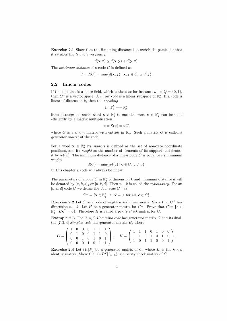
Example 2.3 The [7, 4, 3] Hamming code has generator matrix G and its dual,the [7, 3, 4] Simplex code has generator matrix H, where

G =

1 0 0 0 1 1 10 1 0 0 1 1 00 0 1 0 1 0 10 0 0 1 0 1 1

, H =

1 1 1 0 1 0 01 1 0 1 0 1 01 0 1 1 0 0 1

.

Exercise 2.4 Let (Ik|P ) be a generator matrix of C, where Ik is the k × kidentity matrix. Show that (−PT |In−k) is a parity check matrix of C.

4

2.3 Weight distribution

Apart from the minimum distance, a code has other important invariants. Oneof these is the weight distribution {(i, αi) | i = 0, 1, . . . n}, where αi denotes thenumber of codewords in C of weight i. The polynomials WC(X, Y ) and WC(X),defined as

WC(X, Y ) =n∑

i=0

αiXn−iY i and WC(X) =

n∑i=0

αiXn−i

are called the (homogeneous) weight enumerators of C. Although there is noapparent relation between the minimum distance of a code and its dual, theweight enumerators satisfy the MacWilliams identity.

Theorem 2.5 Let C be an [n, k] code over Fq. Then

WC⊥(X, Y ) = q−kWC(X + (q − 1)Y, X − Y ).

2.4 Automorphisms and isometries of codes

Other important invariants of a code are its group of automorphisms and itsgroup of isometries.

Let Perm(n, q) be the subgroup of GL(n, q) consisting of permutations of co-ordinates. Let Diag(n, q) be the subgroup of GL(n, q) consisting of diagonalmatirices. Let Iso(n, q) be the subgroup of GL(n, q) which is generated byPerm(n, q) and Diag(n, q).

A code that is the image of C under an element of Perm(n, q) is said tobe equivalent to C. The subgroup of Perm(n, q) that leaves C invariant is theautomorphism group of C, Aut(C).

A code that is the image of C under an element of Iso(n, q) is said to beisometric to C. The subgroup of Iso(n, q) that leaves C invariant is the isometrygroup of C, Iso(C).

Exercise 2.6 Show that Aut(C) = Aut(C⊥) and similarly for Iso(C).

Exercise 2.7 Show that a linear map ϕ : Fnq → Fn

q is an isometry if and onlyif ϕ leaves the Hamming metric invariant, that means that

d(ϕ(x), ϕ(y)) = d(x,y)

for all x,y ∈ Fnq .

A code of length n is called cyclic if the cyclic permutation of coordinatesσ(i) = i− 1 modulo n leaves the code invariant. See Section 4.

Exercise 2.8 Show that the [7, 4, 3] Hamming code, as defined in Example 2.3,is not cyclic, but that it is equivalent to a cyclic code.

5

3 Determining the minimum distance

Given a generator matrix of a code, the problem is to determine the minimumdistance of the code. We will give five possible solutions here. All these methodsdo not have polynomial complexity in n, the lenght of the code. One cannothope for a polynomial algorithm, since recently it has been proved that thisproblem is NP complete.

3.1 Exhaustive search

This is the first approach that comes to mind. It is the brute force method:generate all codewords and check for their weights.

Since one generates the whole code, other invariants, like the weight distribution,are easy to determine at the same expence. But going through all codewords isthe most inefficient way of dealing with the problem.

It is not necessary to consider all scalar multiples λc of a codeword c anda nonzero λ ∈ Fq, since they all have the same weight. This improves thecomplexity by a factor q − 1. One can speed up the procedure if one knowsmore about the code at forehand, for example the automorphism group, inparticular for cyclic codes.

By the MacWilliams relations, knowing the weight distribution of a code,one can determine the weight distribution of the dual code by solving linearequations. Therefore it is good to do exhaustive search on whatever code (C orC⊥) has lowest dimension.

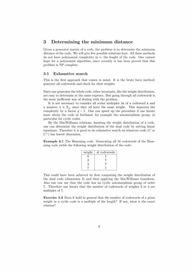
Example 3.1 The Hamming code. Generating all 16 codewords of the Ham-ming code yields the following weight distribution of the code:

weight # codewords0 13 74 77 1

This could have been achieved by first computing the weight distribution ofthe dual code (dimension 3) and then applying the MacWilliams transform.Also one can use that the code has an cyclic automorphism group of order7. Therefore one knows that the number of codewords of weights 3 or 4 aremultiples of 7.

Exercise 3.2 Does it hold in general that the number of codewords of a givenweight in a cyclic code is a multiple of the length? If not, what is the exactrelation?

6

3.2 Linear algebra

In a sense the theory of linear codes is ”just linear algebra”. The determinationof the minimum distance can be phrased in these terms as the following exerciseshows.

Exercise 3.3 The minimum distance is the minimal number of dependentcolumns in a parity check matrix.

But also for this method one has to look at all possible combinations of columns,and this number grows exponentially.

We give a sketch how the minimum distance of linear codes is determined bythe algorithm of Brouwer. Let G be a k × n generator matrix of G. After apermutation of the columns and rowreductions we may suppose that the firstk columns form the k × k identity matrix. Any linear combination of w rowswith non-zero coefficients gives a codeword of weight at least w. In particular,if the code has minimum distance 1, then we will notice this by the fact thatone of the rows of G has weight 1. More generaly, we look at all possible linearcombinations of w rows for w = 1, 2, . . . and keep track of the codeword ofsmallest weight. If we have found a codeword of weight v, then we can restrictthe possible number of rows we have to consider to v − 1. The lower bound wfor the weight of the codewords we generate is raised, and the lowest weight vof a codeword found in the process so far is lowered. Finally v and w meet.

An improvement of this method is obtained if G is of the form (G1 · · ·Gl)where G1, . . . , Gl are matrices such that the first k columns of Gj form thek × k identity matrix for all j = 1, . . . , l. In this way we know that any linearcombination of w rows with non-zero coefficients gives a codeword of weight atleast lw.

Exercise 3.4 Show that the maximum length of a binary code of dimension4 and dual distance 3 is 7. What is the maximum length of a q-ary code ofdimension k and dual distance 3 ? Hint: use Exercise 3.3 and read the nextsection on finite geometry first.

3.3 Finite geometry

It is possible to give the minimum distance of a code a geometric interpretation.

Suppose that the code is nondegenerate, this means that there is not a coordinatej such that cj = 0 for all codewords c. For the determination of the minimumdistance this is not an important restriction. So every column of the generatormatrix G of a [n, k, d] code is not zero and its homogeneous coordinates can beconsidered as a point in projective space of dimension k − 1 over Fq. If twocolumns are dependent, then they give rise to the same point. In this way weget a set P of n points (counted with multplicities) in PG(k − 1, q), that arenot all contained in a hyperplane. This is called a projective system.

7

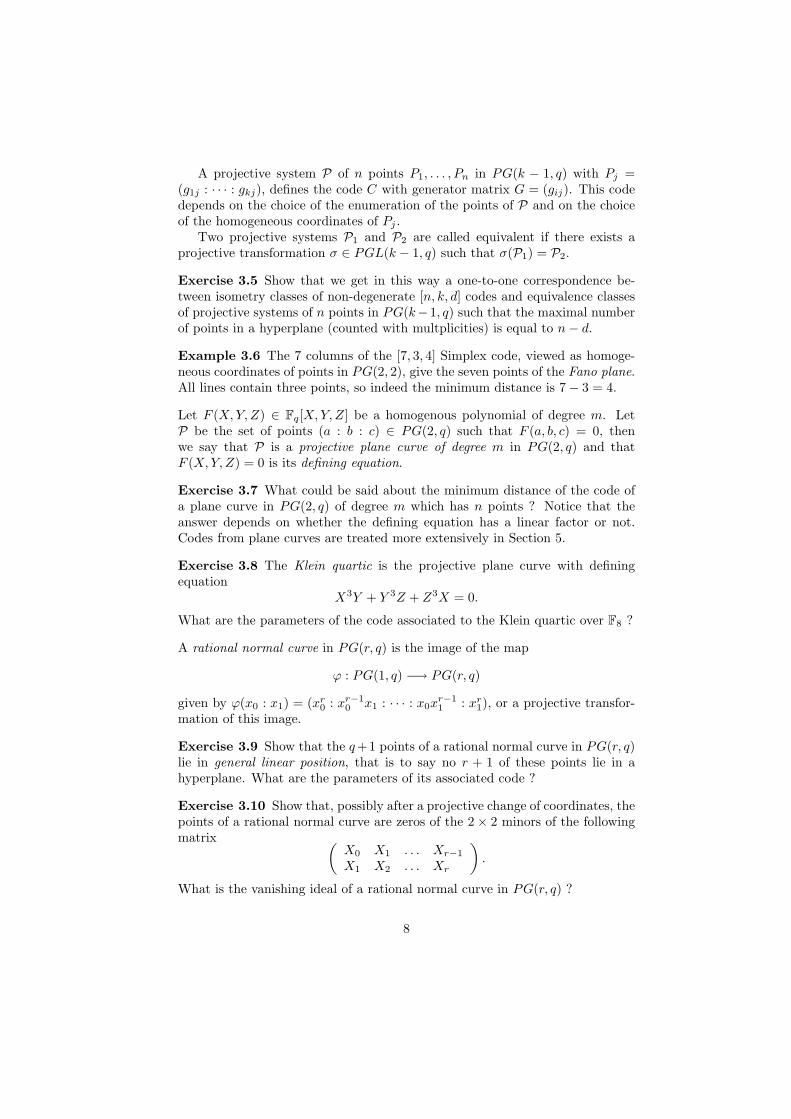
A projective system P of n points P1, . . . , Pn in PG(k − 1, q) with Pj =(g1j : · · · : gkj), defines the code C with generator matrix G = (gij). This codedepends on the choice of the enumeration of the points of P and on the choiceof the homogeneous coordinates of Pj .

Two projective systems P1 and P2 are called equivalent if there exists aprojective transformation σ ∈ PGL(k − 1, q) such that σ(P1) = P2.

Exercise 3.5 Show that we get in this way a one-to-one correspondence be-tween isometry classes of non-degenerate [n, k, d] codes and equivalence classesof projective systems of n points in PG(k−1, q) such that the maximal numberof points in a hyperplane (counted with multplicities) is equal to n− d.

Example 3.6 The 7 columns of the [7, 3, 4] Simplex code, viewed as homoge-neous coordinates of points in PG(2, 2), give the seven points of the Fano plane.All lines contain three points, so indeed the minimum distance is 7− 3 = 4.

Let F (X, Y, Z) ∈ Fq[X, Y, Z] be a homogenous polynomial of degree m. LetP be the set of points (a : b : c) ∈ PG(2, q) such that F (a, b, c) = 0, thenwe say that P is a projective plane curve of degree m in PG(2, q) and thatF (X, Y, Z) = 0 is its defining equation.

Exercise 3.7 What could be said about the minimum distance of the code ofa plane curve in PG(2, q) of degree m which has n points ? Notice that theanswer depends on whether the defining equation has a linear factor or not.Codes from plane curves are treated more extensively in Section 5.

Exercise 3.8 The Klein quartic is the projective plane curve with definingequation

X3Y + Y 3Z + Z3X = 0.

What are the parameters of the code associated to the Klein quartic over F8 ?

A rational normal curve in PG(r, q) is the image of the map

ϕ : PG(1, q) −→ PG(r, q)

given by ϕ(x0 : x1) = (xr0 : xr−1

0 x1 : · · · : x0xr−11 : xr

1), or a projective transfor-mation of this image.

Exercise 3.9 Show that the q+1 points of a rational normal curve in PG(r, q)lie in general linear position, that is to say no r + 1 of these points lie in ahyperplane. What are the parameters of its associated code ?

Exercise 3.10 Show that, possibly after a projective change of coordinates, thepoints of a rational normal curve are zeros of the 2× 2 minors of the followingmatrix (

X0 X1 . . . Xr−1

X1 X2 . . . Xr

).

What is the vanishing ideal of a rational normal curve in PG(r, q) ?

8

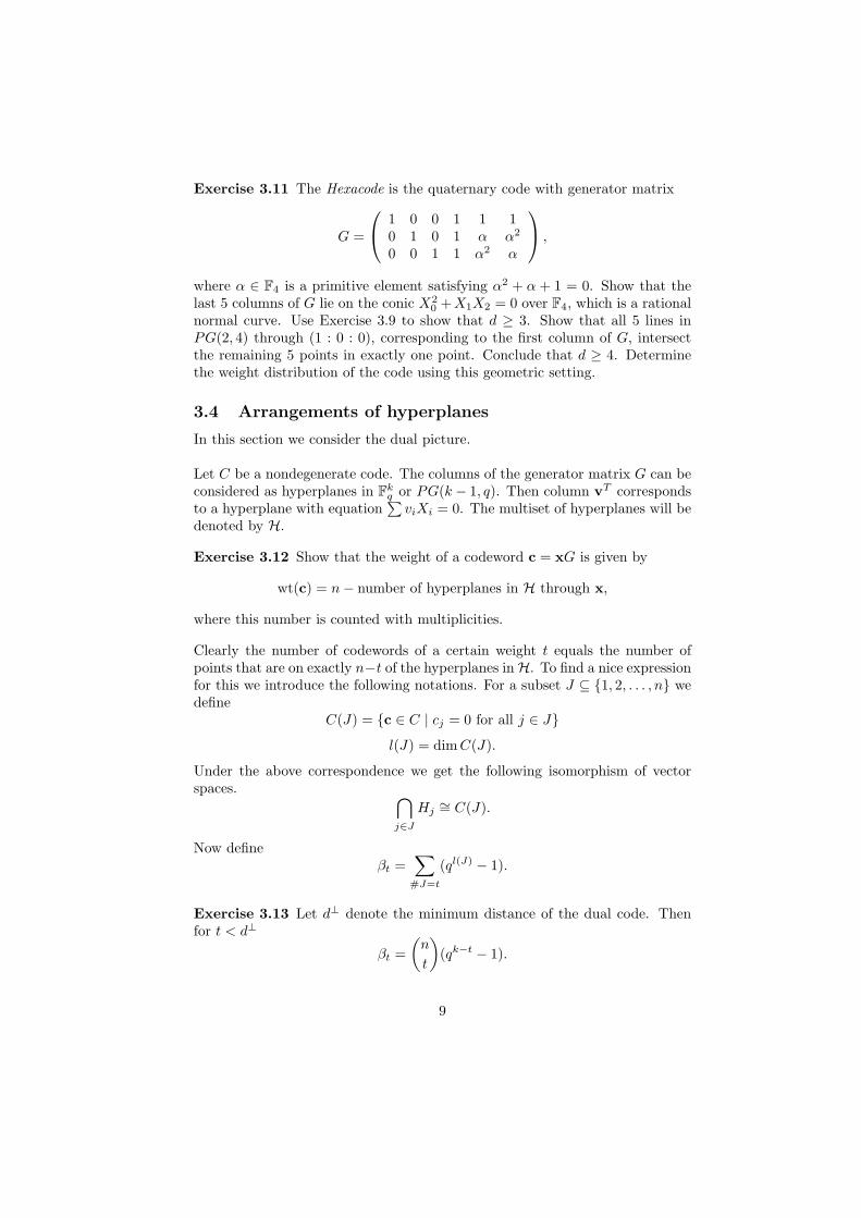
Exercise 3.11 The Hexacode is the quaternary code with generator matrix

G =

1 0 0 1 1 10 1 0 1 α α2

0 0 1 1 α2 α

,

where α ∈ F4 is a primitive element satisfying α2 + α + 1 = 0. Show that thelast 5 columns of G lie on the conic X2

0 +X1X2 = 0 over F4, which is a rationalnormal curve. Use Exercise 3.9 to show that d ≥ 3. Show that all 5 lines inPG(2, 4) through (1 : 0 : 0), corresponding to the first column of G, intersectthe remaining 5 points in exactly one point. Conclude that d ≥ 4. Determinethe weight distribution of the code using this geometric setting.

3.4 Arrangements of hyperplanes

In this section we consider the dual picture.

Let C be a nondegenerate code. The columns of the generator matrix G can beconsidered as hyperplanes in Fk

q or PG(k − 1, q). Then column vT correspondsto a hyperplane with equation

∑viXi = 0. The multiset of hyperplanes will be

denoted by H.

Exercise 3.12 Show that the weight of a codeword c = xG is given by

wt(c) = n− number of hyperplanes in H through x,

where this number is counted with multiplicities.

Clearly the number of codewords of a certain weight t equals the number ofpoints that are on exactly n−t of the hyperplanes inH. To find a nice expressionfor this we introduce the following notations. For a subset J ⊆ {1, 2, . . . , n} wedefine

C(J) = {c ∈ C | cj = 0 for all j ∈ J}

l(J) = dim C(J).

Under the above correspondence we get the following isomorphism of vectorspaces. ⋂

j∈J

Hj∼= C(J).

Now defineβt =

∑#J=t

(ql(J) − 1).

Exercise 3.13 Let d⊥ denote the minimum distance of the dual code. Thenfor t < d⊥

βt =(

n

t

)(qk−t − 1).

9

Exercise 3.14 Recall that αs is the number of codewords of weight s. Provethe following formula

βt =n−t∑s=d

(n− s

t

)αs.

by computing the number of elements of the set of pairs

{(J, c) | J ⊆ {1, 2, . . . , n},#J = t, c ∈ C(J), c 6= 0}

in two different ways.

Exercise 3.15 Show that the weight enumerator of C can be expressed in termsof the βt as follows.

WC(X) = Xn +n−d∑t=0

βt(X − 1)t.

Exercise 3.16 Prove the following identity either by inverting the formula ofExercise 3.14 or by an inclusion/exclusion argument.

αs =n−d∑

t=n−s

(−1)n+s+t

(t

n− s

)βt.

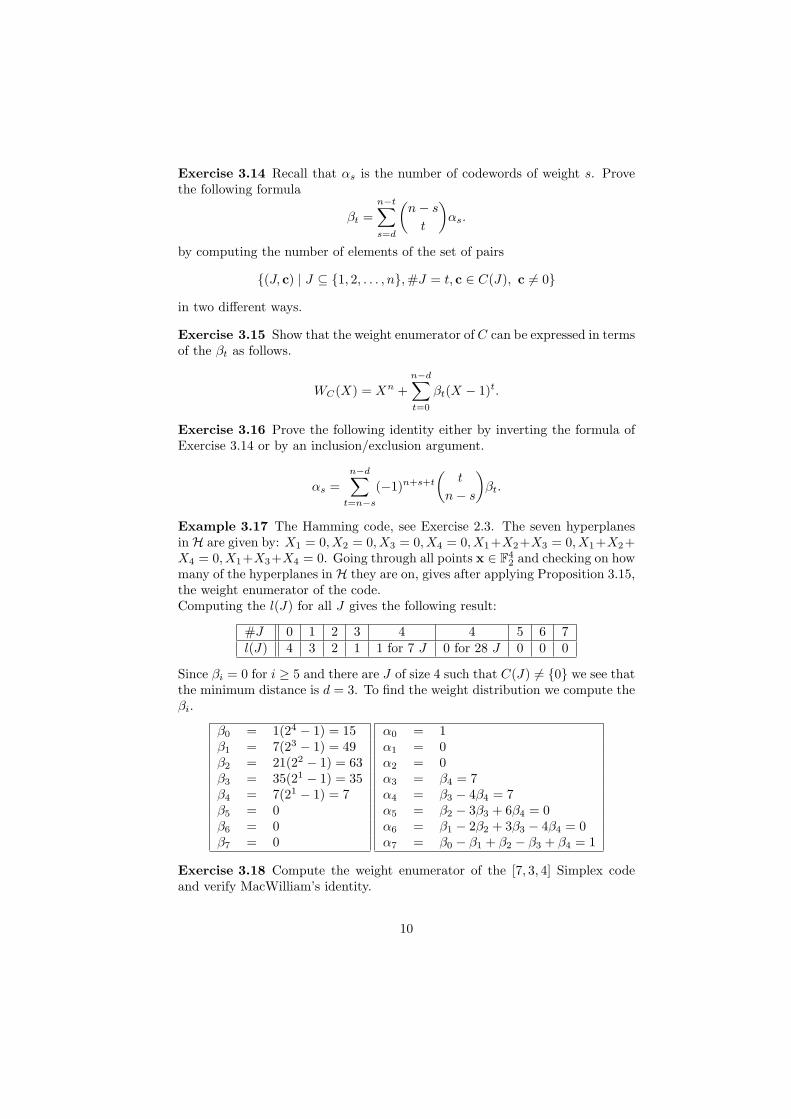
Example 3.17 The Hamming code, see Exercise 2.3. The seven hyperplanesin H are given by: X1 = 0, X2 = 0, X3 = 0, X4 = 0, X1+X2+X3 = 0, X1+X2+X4 = 0, X1+X3+X4 = 0. Going through all points x ∈ F4

2 and checking on howmany of the hyperplanes in H they are on, gives after applying Proposition 3.15,the weight enumerator of the code.Computing the l(J) for all J gives the following result:

#J 0 1 2 3 4 4 5 6 7l(J) 4 3 2 1 1 for 7 J 0 for 28 J 0 0 0

Since βi = 0 for i ≥ 5 and there are J of size 4 such that C(J) 6= {0} we see thatthe minimum distance is d = 3. To find the weight distribution we compute theβi.

β0 = 1(24 − 1) = 15β1 = 7(23 − 1) = 49β2 = 21(22 − 1) = 63β3 = 35(21 − 1) = 35β4 = 7(21 − 1) = 7β5 = 0β6 = 0β7 = 0

α0 = 1α1 = 0α2 = 0α3 = β4 = 7α4 = β3 − 4β4 = 7α5 = β2 − 3β3 + 6β4 = 0α6 = β1 − 2β2 + 3β3 − 4β4 = 0α7 = β0 − β1 + β2 − β3 + β4 = 1

Exercise 3.18 Compute the weight enumerator of the [7, 3, 4] Simplex codeand verify MacWilliam’s identity.

10

Exercise 3.19 Compute the weight enumerator of the code on the Klein quar-tic of Exercise 3.8.

Exercise 3.20 Let C be an [n, k, n − k + 1] code. Show that l(J) = n − #Jfor all J . Compute the weight enumerator of such a code.

Exercise 3.21 Prove that the number l(J) is the same for the codes C andFqeC in Fn

qe for any extension Fqe of Fq.

Using the Exercises 3.14, 3.16 and 3.21 it is immediate to find the weight distri-bution of a code over any extension Fqe if one knows the l(J) over the groundfield Fq for all subsets J of {1, . . . , n}. Computing the C(J) and l(J) for a fixedJ is just linear algebra. The large complexity for the computation of the weightenumerator and the minimum distance in this way stems from the exponentialgrowth of the number of all possible subsets of {1, . . . , n}.

Exercise 3.22 Let C be the code over Fq, with q even, with generator matrixH of Exercise 2.3. For which q does this code contain a word of weight 7 ?

Exercise 3.23 Compare the complexity of the methods ”exhaustive search”and ”arrangements of hyperplanes” to compute the weight enumerator as afunction of q and the parameters [n, k, d] and d⊥.

3.5 Algebra

Let the n hyperplanes in H have equations

L1(X) = L2(X) = · · · = Ln(X) = 0,

where the Li are linear forms in the variables X1, X2, . . . , Xk as in the previoussection. Then a general codeword is of the form

c = (L1(x), L2(x), . . . , Ln(x)),

where x ∈ Fkq . Now let It be the ideal generated by all products of t distinct

Li(X), so

It =

(t∏

s=1

Lis(X) | 1 ≤ i1 < i2 < · · · < it ≤ n

).

If Φt is the ideal generated by all homogeneous forms of degree t in k variablesX1, . . . , Xk, then clearly It ⊆ Φt. We have the following.

Exercise 3.24 Show that

V (It, Fq) = {x ∈ Fkq | wt(c) < t, with c = xG}.

Exercise 3.25 Show that

d = min{t | V (It+1, Fq) 6= {0}}.

11

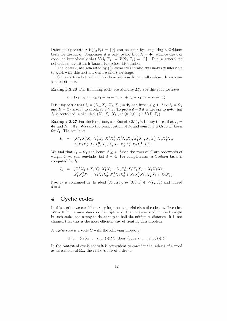
Determining whether V (It, Fq) = {0} can be done by computing a Grobnerbasis for the ideal. Sometimes it is easy to see that It = Φt, whence one canconclude immediately that V (It, Fq) = V (Φt, Fq) = {0}. But in general nopolynomial algorithm is known to decide this question.

The ideals It are generated by(nt

)elements and also this makes it infeasible

to work with this method when n and t are large.Contrary to what is done in exhaustive search, here all codewords are con-

sidered at once.

Example 3.26 The Hamming code, see Exercise 2.3. For this code we have

c = (x1, x2, x3, x4, x1 + x2 + x3, x1 + x2 + x4, x1 + x3 + x4).

It is easy to see that I1 = (X1, X2, X3, X4) = Φ1 and hence d ≥ 1. Also I2 = Φ2

and I3 = Φ3 is easy to check, so d ≥ 3. To prove d = 3 it is enough to note thatI4 is contained in the ideal (X1, X2, X3), so (0, 0, 0, 1) ∈ V (I4, F2).

Example 3.27 For the Hexacode, see Exercise 3.11, it is easy to see that I1 =Φ1 and I2 = Φ2. We skip the computation of I3 and compute a Grobner basisfor I4. The result is:

I4 = (X41 , X3

1X2, X31X3, X

21X2

2 , X21X2X3, X

21X2

3 , X1X32 , X1X

22X3,

X1X2X23 , X1X

33 , X4

2 , X32X3, X

22X2

3 , X2X33 , X4

3 ).

We find that I4 = Φ4 and hence d ≥ 4. Since the rows of G are codewords ofweight 4, we can conclude that d = 4. For completeness, a Grobner basis iscomputed for I5:

I5 = (X41X2 + X1X

42 , X4

1X3 + X1X43 , X3

1X2X3 + X1X22X2

3 ,

X21X2

2X3 + X1X2X33 , X2

1X2X23 + X1X

32X3, X

42X3 + X2X

43 ).

Now I5 is contained in the ideal (X1, X2), so (0, 0, 1) ∈ V (I5, F4) and indeedd = 4.

4 Cyclic codes

In this section we consider a very important special class of codes: cyclic codes.We will find a nice algebraic description of the codewords of minimal weightin such codes and a way to decode up to half the minimum distance. It is notclaimed that this is the most efficient way of treating this problem.

A cyclic code is a code C with the following property:

if c = (c0, c1 . . . , cn−1) ∈ C, then (cn−1, c0 . . . , cn−2) ∈ C.

In the context of cyclic codes it is convenient to consider the index i of a wordas an element of Zn, the cyclic group of order n.

12

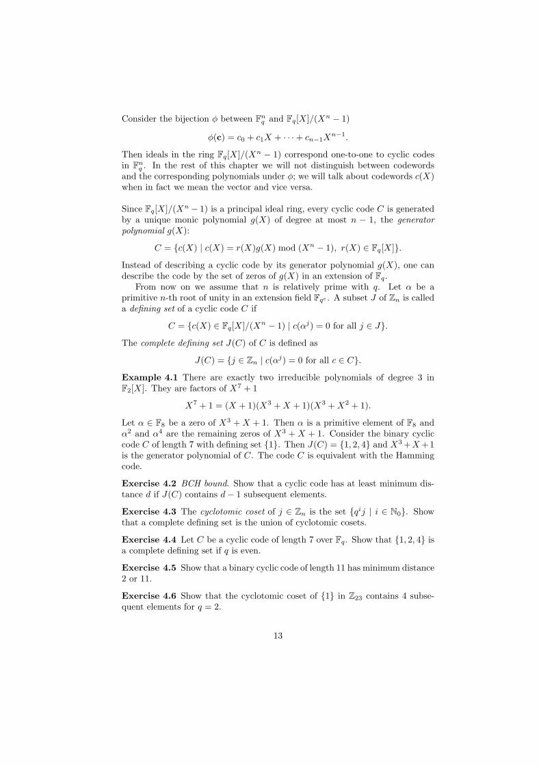
Consider the bijection φ between Fnq and Fq[X]/(Xn − 1)

φ(c) = c0 + c1X + · · ·+ cn−1Xn−1.

Then ideals in the ring Fq[X]/(Xn − 1) correspond one-to-one to cyclic codesin Fn

q . In the rest of this chapter we will not distinguish between codewordsand the corresponding polynomials under φ; we will talk about codewords c(X)when in fact we mean the vector and vice versa.

Since Fq[X]/(Xn − 1) is a principal ideal ring, every cyclic code C is generatedby a unique monic polynomial g(X) of degree at most n − 1, the generatorpolynomial g(X):

C = {c(X) | c(X) = r(X)g(X) mod (Xn − 1), r(X) ∈ Fq[X]}.

Instead of describing a cyclic code by its generator polynomial g(X), one candescribe the code by the set of zeros of g(X) in an extension of Fq.

From now on we assume that n is relatively prime with q. Let α be aprimitive n-th root of unity in an extension field Fqe . A subset J of Zn is calleda defining set of a cyclic code C if

C = {c(X) ∈ Fq[X]/(Xn − 1) | c(αj) = 0 for all j ∈ J}.

The complete defining set J(C) of C is defined as

J(C) = {j ∈ Zn | c(αj) = 0 for all c ∈ C}.

Example 4.1 There are exactly two irreducible polynomials of degree 3 inF2[X]. They are factors of X7 + 1

X7 + 1 = (X + 1)(X3 + X + 1)(X3 + X2 + 1).

Let α ∈ F8 be a zero of X3 + X + 1. Then α is a primitive element of F8 andα2 and α4 are the remaining zeros of X3 + X + 1. Consider the binary cycliccode C of length 7 with defining set {1}. Then J(C) = {1, 2, 4} and X3 +X +1is the generator polynomial of C. The code C is equivalent with the Hammingcode.

Exercise 4.2 BCH bound. Show that a cyclic code has at least minimum dis-tance d if J(C) contains d− 1 subsequent elements.

Exercise 4.3 The cyclotomic coset of j ∈ Zn is the set {qij | i ∈ N0}. Showthat a complete defining set is the union of cyclotomic cosets.

Exercise 4.4 Let C be a cyclic code of length 7 over Fq. Show that {1, 2, 4} isa complete defining set if q is even.

Exercise 4.5 Show that a binary cyclic code of length 11 has minimum distance2 or 11.

Exercise 4.6 Show that the cyclotomic coset of {1} in Z23 contains 4 subse-quent elements for q = 2.

13

4.1 The Mattson-Solomon polynomial

Let a(X) be a word in Fnq . Let α ∈ Fqe be a primitive n-th root of unity. Then

the Mattson-Solomon (MS) polynomial of a(X) is defined as

A(Z) =n∑

i=1

AiZn−i, Ai = a(αi) ∈ Fqe .

Here too we adopt the convention that the index i is an element of Zn, soAn+i = Ai.

The MS polynomial A(Z) is the discrete Fourier transform of the word a(X).Notice that An ∈ Fq.

Proposition 4.71. The inverse is given by aj = 1

nA(αj).2. A(z) is the MS polynomial of a word a(X) if and only if Ajq = Aq

j for allj ∈ Zn.3. A(z) is the MS polynomial of a codeword a(X) of the cyclic code C if andonly if Aj = 0 for all j ∈ J(C) and Ajq = Aq

j for all j = 1, . . . , n.

Exercise 4.8 Let β ∈ Fqe be a zero of Xn − 1. Show thatn∑

i=1

βi ={

n if β = 10 if β 6= 1.

Expand A(αi) using the definitions and use the above fact to prove Proposition4.7(1). Prove the remaining assertions of Proposition 4.7.

Let a(X) be a word of weight w. Then the locators x1, x2, . . . , xw of a(X) aredefined as

{x1, x2, . . . , xw} = {αi | ai 6= 0}.Let yj = ai if xj = αi. Then

Ai = a(αi) =w∑

j=1

yjxij .

Consider the product

σ(Z) =w∏

j=1

(1− xjZ).

Then σ(Z) has as zeros the reciprocals of the locators, and is sometimes calledthe locator polynomial. In this chapter and the following on decoding this nameis reserved for the polynomial that has the locators as zeros.

Let σ(Z) =∑w

i=0 σiZi. Then σi is the ith elementary symmetric function

in these locators:

σt = (−1)t∑

1≤j1<j2<···<jt≤w

xj1xj2 · · ·xjt.

14

The following property of the MS polynomial is called the generalized Newtonidentity and gives the reason for these definitions.

Proposition 4.9 For all i it holds that

Ai+w + σ1Ai+w−1 + · · ·+ σwAi = 0.

Exercise 4.10 Substitute Z = 1/xj in the equation

1 + σ1Z + · · ·+ σwZw =w∏

j=1

(1− xjZ)

and multiply by yjxi+wj . This gives

yjxi+wj + σ1yjx

i+w−1j + · · ·+ σwyjx

ij = 0.

Check that summing on j = 1, . . . , w yields the desired result of Proposition4.9.

Example 4.11 Let C be the cyclic code of length 5 over F16 with defining set{1, 2}. Then this defining set is complete. The polynomial

X4 + X3 + X2 + X + 1

is irreducible over F2. Let β be a zero of this polynomial in F16. Then the orderof β is 5. The generator polynomial of C is

(X + β)(X + β2) = X2 + (β + β2)X + β3.

So (β3, β + β2, 1, 0, 0) ∈ C and

(β + β2 + β3, 1 + β, 0, 1, 0) = (β + β2)(β3, β + β2, 1, 0, 0) + (0, β3, β + β2, 1, 0)

is an element of C. These codewords together with their cyclic shifts and theirnonzero scalar multiples give (5 + 5) ∗ 15 = 150 words of weight 3.

Using Propositions 4.7 and 4.9 it will be shown that these are the onlycodewords of weight 3. Consider the set of equations:

A4 + σ1A3 + σ2A2 + σ3A1 = 0A5 + σ1A4 + σ2A3 + σ3A2 = 0A1 + σ1A5 + σ2A4 + σ3A3 = 0A2 + σ1A1 + σ2A5 + σ3A4 = 0A3 + σ1A2 + σ2A1 + σ3A5 = 0

If A1, A2, A3, A4 and A5 are the coefficients of the MS polynomial of a codeword,then A1 = A2 = 0. If A3 = 0, then Ai = 0 for all i. So we may assume thatA3 6= 0. The above equations imply A4 = σ1A3, A5 = (σ2

1 + σ2)A3 and σ31 + σ3 = 0

σ21σ2 + σ2

2 + σ1σ3 = 0σ2

1σ3 + σ2σ3 + 1 = 0.

15

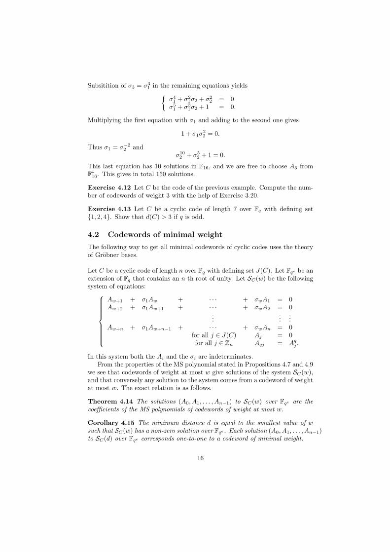
Subsitition of σ3 = σ31 in the remaining equations yields{

σ41 + σ2

1σ2 + σ22 = 0

σ51 + σ3

1σ2 + 1 = 0.

Multiplying the first equation with σ1 and adding to the second one gives

1 + σ1σ22 = 0.

Thus σ1 = σ−22 and

σ102 + σ5

2 + 1 = 0.

This last equation has 10 solutions in F16, and we are free to choose A3 fromF∗16. This gives in total 150 solutions.

Exercise 4.12 Let C be the code of the previous example. Compute the num-ber of codewords of weight 3 with the help of Exercise 3.20.

Exercise 4.13 Let C be a cyclic code of length 7 over Fq with defining set{1, 2, 4}. Show that d(C) > 3 if q is odd.

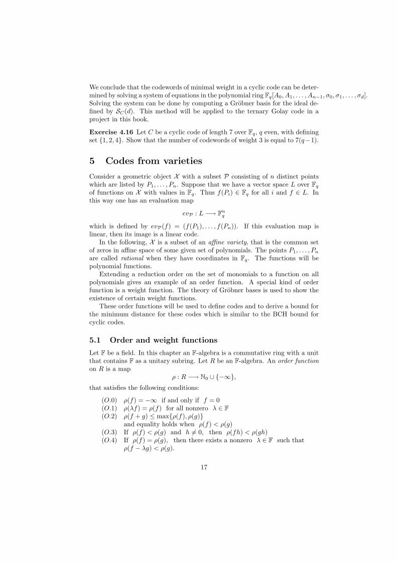
4.2 Codewords of minimal weight

The following way to get all minimal codewords of cyclic codes uses the theoryof Grobner bases.

Let C be a cyclic code of length n over Fq with defining set J(C). Let Fqe be anextension of Fq that contains an n-th root of unity. Let SC(w) be the followingsystem of equations:

Aw+1 + σ1Aw + · · · + σwA1 = 0Aw+2 + σ1Aw+1 + · · · + σwA2 = 0

......

...Aw+n + σ1Aw+n−1 + · · · + σwAn = 0

for all j ∈ J(C) Aj = 0for all j ∈ Zn Aqj = Aq

j .

In this system both the Ai and the σi are indeterminates.From the properties of the MS polynomial stated in Propositions 4.7 and 4.9

we see that codewords of weight at most w give solutions of the system SC(w),and that conversely any solution to the system comes from a codeword of weightat most w. The exact relation is as follows.

Theorem 4.14 The solutions (A0, A1, . . . , An−1) to SC(w) over Fqe are thecoefficients of the MS polynomials of codewords of weight at most w.

Corollary 4.15 The minimum distance d is equal to the smallest value of wsuch that SC(w) has a non-zero solution over Fqe . Each solution (A0, A1, . . . , An−1)to SC(d) over Fqe corresponds one-to-one to a codeword of minimal weight.

16

We conclude that the codewords of minimal weight in a cyclic code can be deter-mined by solving a system of equations in the polynomial ring Fq[A0, A1, . . . , An−1, σ0, σ1, . . . , σd].Solving the system can be done by computing a Grobner basis for the ideal de-fined by SC(d). This method will be applied to the ternary Golay code in aproject in this book.

Exercise 4.16 Let C be a cyclic code of length 7 over Fq, q even, with definingset {1, 2, 4}. Show that the number of codewords of weight 3 is equal to 7(q−1).

5 Codes from varieties

Consider a geometric object X with a subset P consisting of n distinct pointswhich are listed by P1, . . . , Pn. Suppose that we have a vector space L over Fq

of functions on X with values in Fq. Thus f(Pi) ∈ Fq for all i and f ∈ L. Inthis way one has an evaluation map

evP : L −→ Fnq

which is defined by evP(f) = (f(P1), . . . , f(Pn)). If this evaluation map islinear, then its image is a linear code.

In the following, X is a subset of an affine variety, that is the common setof zeros in affine space of some given set of polynomials. The points P1, . . . , Pn

are called rational when they have coordinates in Fq. The functions will bepolynomial functions.

Extending a reduction order on the set of monomials to a function on allpolynomials gives an example of an order function. A special kind of orderfunction is a weight function. The theory of Grobner bases is used to show theexistence of certain weight functions.

These order functions will be used to define codes and to derive a bound forthe minimum distance for these codes which is similar to the BCH bound forcyclic codes.

5.1 Order and weight functions

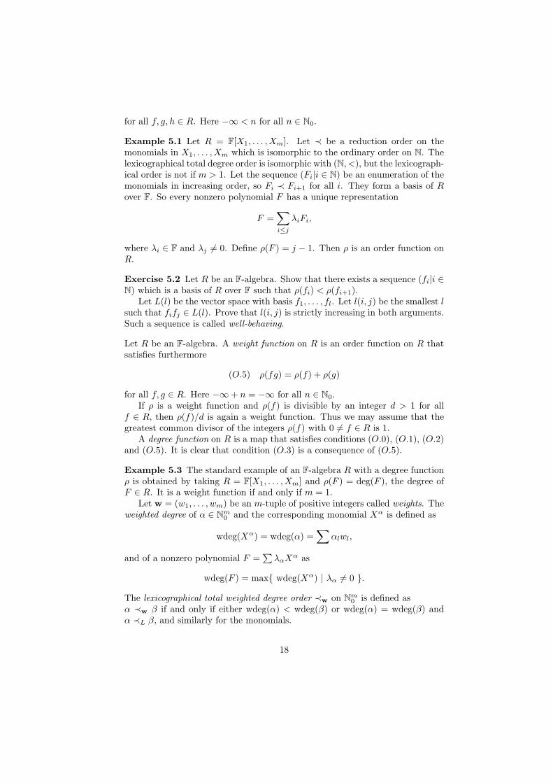
Let F be a field. In this chapter an F-algebra is a commutative ring with a unitthat contains F as a unitary subring. Let R be an F-algebra. An order functionon R is a map

ρ : R −→ N0 ∪ {−∞},that satisfies the following conditions:

(O.0) ρ(f) = −∞ if and only if f = 0(O.1) ρ(λf) = ρ(f) for all nonzero λ ∈ F(O.2) ρ(f + g) ≤ max{ρ(f), ρ(g)}

and equality holds when ρ(f) < ρ(g)(O.3) If ρ(f) < ρ(g) and h 6= 0, then ρ(fh) < ρ(gh)(O.4) If ρ(f) = ρ(g), then there exists a nonzero λ ∈ F such that

ρ(f − λg) < ρ(g).

17

for all f, g, h ∈ R. Here −∞ < n for all n ∈ N0.

Example 5.1 Let R = F[X1, . . . , Xm]. Let ≺ be a reduction order on themonomials in X1, . . . , Xm which is isomorphic to the ordinary order on N. Thelexicographical total degree order is isomorphic with (N, <), but the lexicograph-ical order is not if m > 1. Let the sequence (Fi|i ∈ N) be an enumeration of themonomials in increasing order, so Fi ≺ Fi+1 for all i. They form a basis of Rover F. So every nonzero polynomial F has a unique representation

F =∑i≤j

λiFi,

where λi ∈ F and λj 6= 0. Define ρ(F ) = j − 1. Then ρ is an order function onR.

Exercise 5.2 Let R be an F-algebra. Show that there exists a sequence (fi|i ∈N) which is a basis of R over F such that ρ(fi) < ρ(fi+1).

Let L(l) be the vector space with basis f1, . . . , fl. Let l(i, j) be the smallest lsuch that fifj ∈ L(l). Prove that l(i, j) is strictly increasing in both arguments.Such a sequence is called well-behaving.

Let R be an F-algebra. A weight function on R is an order function on R thatsatisfies furthermore

(O.5) ρ(fg) = ρ(f) + ρ(g)

for all f, g ∈ R. Here −∞+ n = −∞ for all n ∈ N0.If ρ is a weight function and ρ(f) is divisible by an integer d > 1 for all

f ∈ R, then ρ(f)/d is again a weight function. Thus we may assume that thegreatest common divisor of the integers ρ(f) with 0 6= f ∈ R is 1.

A degree function on R is a map that satisfies conditions (O.0), (O.1), (O.2)and (O.5). It is clear that condition (O.3) is a consequence of (O.5).

Example 5.3 The standard example of an F-algebra R with a degree functionρ is obtained by taking R = F[X1, . . . , Xm] and ρ(F ) = deg(F ), the degree ofF ∈ R. It is a weight function if and only if m = 1.

Let w = (w1, . . . , wm) be an m-tuple of positive integers called weights. Theweighted degree of α ∈ Nm

0 and the corresponding monomial Xα is defined as

wdeg(Xα) = wdeg(α) =∑

αlwl,

and of a nonzero polynomial F =∑

λαXα as

wdeg(F ) = max{ wdeg(Xα) | λα 6= 0 }.

The lexicographical total weighted degree order ≺w on Nm0 is defined as

α ≺w β if and only if either wdeg(α) < wdeg(β) or wdeg(α) = wdeg(β) andα ≺L β, and similarly for the monomials.

18

Exercise 5.4 Show that wdeg is a degree function on F[X1, . . . , Xm] and that≺w is a reduction order that is isomorphic with (N, <).

Exercise 5.5 Let R be an F-algebra with a weight function. Show that the setof elements of weight zero is equal to F∗.

Example 5.6 Consider the F-algebra

R = F[X, Y ]/(X5 − Y 4 − Y ).

Assume that R has a weight function ρ. Let x and y be the cosets in R of Xand Y , respectively. Then x5 = y4 + y. Now y 6∈ F, so ρ(y) > 0 by Exercise 5.5,and ρ(y4) = 4ρ(y) > ρ(y) by (O.5). Thus ρ(y4 +y) = ρ(y4) by (O.2). Therefore

5ρ(x) = ρ(x5) = ρ(y4 + y) = 4ρ(y)

Thus the only possible solution is ρ(x) = 4 and ρ(y) = 5.

Exercise 5.7 Let R = F[X, Y ]/(X3Y + Y 3 + X). Show by the same reasoningas in the example above that ρ(x) = 2 and ρ(y) = 3 if there exists a weightfunction ρ on R. Prove that there exists no weight function on R.

Let M be the set of monomials in X1, . . . , Xm. The footprint or ∆-set of afinite set B of polynomials is defined by

∆(B) = M\ {lm(BM)|B ∈ B, B 6= 0,M ∈M}.

If B is a Grobner basis for the ideal I in R, then the cosets modulo I of theelements of the footprint ∆(B) form a basis of R/I.

Exercise 5.8 Let ≺w be the lexicographical total weighted degree order on themonomials in X and Y with weights 4 and 5 for X and Y , respectively. Showthat

{XiY j |i, j ∈ N0, j < 4}is the footprint of X5 + Y 4 + Y with respect to the reduction order ≺w.

Prove that the degree function wdeg is injective on this footprint. Let (Fl|l ∈N) be an enumeration of this footprint such that wdeg(Fl) < wdeg(Fl+1) forall l. Let R = F[X, Y ]/(X5 + Y 4 + Y ). Let fi be the coset of Fi in R. Thus(fl|l ∈ N) is a basis of R over F. Define ρl = 4i + 5j if fl = xiyj .

Let L(l) be the vector space with f1, . . . , fl as basis. Let l(i, j) be the smallestl such that fifj ∈ L(l). Prove that ρl = ρi + ρj if l = l(i, j).

Show that there exists a weight function on R as a conclusion of the aboveresults or as a special case of the following.

Theorem 5.9 Let I be an ideal in F[X1, . . . , Xm] with Grobner basis B withrespect to ≺w. Suppose that the elements of the footprint of I have mutuallydistinct weighted degrees and that every element of B has two monomials ofhighest weighted degree in its support. Then there exists a weight function ρ onR = F[X1, . . . , Xm]/I with the property that ρ(f) = wdeg(F ), where f is thecoset of F modulo I, for all polynomials F .

19

Exercise 5.10 Let R = F[X, Y ]/(Xa +Y b +G(X, Y )), where gcd(a, b) = 1 anddeg(G) < b < a. Show that R has a weight function ρ such that ρ(x) = b andρ(y) = a.

Exercise 5.11 Let ρ be a weight function. Let Γ = {ρ(f)|f ∈ R, f 6= 0}.We may assume that the greatest common divisor of Γ is 1. Then Γ is calledthe set of non-gaps, and the complement of Γ in N0 is the set of gaps. Showthat the number of gaps of the weight function of Example 5.10 is equal to(a− 1)(b− 1)/2.

5.2 A bound on the minimum distance

We denote the coordinatewise multiplication on Fnq by ∗. Thus a∗b = (a1b1, . . . , anbn)

for a = (a1, . . . , an) and b = (b1, . . . , bn). The vector space Fnq becomes an Fq-

algebra with the multiplication ∗.

Let R be an affine Fq-algebra. That is to say R = Fq[X1, . . . , Xm]/I, where Iis an ideal of Fq[X1, . . . , Xm]. Let P = {P1, . . . , Pn} consist of n distinct pointsof the zero set of I in Fm

q . Consider the evaluation map

evP : R −→ Fnq ,

defined as evP(f) = (f(P1), . . . , f(Pn)).

Exercise 5.12 Show that evP is well defined and a morphism of Fq-algebras,that means that this map is Fq-linear and evP(fg) = evP(f) ∗ evP(g) for allf, g ∈ R. Prove that the evaluation map is surjective.

Assume that R has an order function ρ. Then there exists a well-behavingsequence (fi | i ∈ N) of R over Fq by Exercise 5.2. So ρ(fi) < ρ(fi+1) for all i.Let hi = evP(fi). Define

C(l) = {c ∈ Fnq |c · hj = 0 for all j ≤ l}.

The map evP is surjective, so there exists an N such that C(l) = 0 for all l ≥ N .

Let y ∈ Fnq . Consider

sij(y) = y · (hi ∗ hj).

Then S(y) = (sij(y)|1 ≤ i, j ≤ N) is the matrix of syndromes of y.

Exercise 5.13 Prove that

S(y) = HDHT ,

where D is the n×n diagonal matrix with y on the diagonal and H is the N×nmatrix with rows h1, . . . ,hN . Use this fact to show that

rank S(y) = wt(y).

20

Let L(l) be the vector space with basis f1, . . . , fl. Let l(i, j) be the smallest lsuch that fifj ∈ L(l). Define

N(l) = {(i, j) | l(i, j) = l + 1}.

Let ν(l) be the number of elements of N(l).

Exercise 5.14 Show that i1 < · · · < it ≤ r and jt < · · · < j1 ≤ r, if(i1, j1), . . . , (it, jt) is an enumeration of the elements of N(l) in increasing orderwith respect to the lexicographical order.

Exercise 5.15 Suppose that y ∈ C(l) \ C(l + 1). Prove that

siujv(y) =

{0 if u + v ≤ tnot zero if u + v = t + 1.

Use this fact together with Exercises 5.13 and 5.14 to prove that

wt(y) ≥ ν(l).

DefinedORD(l) = min{ν(l′)|l′ ≤ l}

dORD,P(l) = min{ν(l′)|l′ ≥ l, C(l′) 6= C(l′ + 1)}.As a consequence of the definitions and Exercise 5.15 we get the following the-orem.

Theorem 5.16 The numbers dORD,P(l) and dORD(l) are lower bounds for theminimum distance of C(l):

d(C(l)) ≥ dORD,P(l) ≥ dORD(l).

Exercise 5.17 Reed-Solomon codes. Let R = Fq[X]. Let ρ be the order func-tion defined as ρ(f) = deg(f). Let α be a primitive element of Fq. Let n = q−1and P = {α0, . . . , αn−1}.

Prove that (Xi−1|i ∈ N) is a well-behaving sequence and l(i, j) = i + j − 1.Show that C(l) is a cyclic code with defining set {0, 1, . . . , l−1} and dORD(l) =

l + 1. Thus the BCH bound is obtained.

Exercise 5.18 Let ρ be a weight function and (fi|i ∈ N) a well-behaving se-quence. Let ρi = ρ(fi). Show that N(l) = {(i, j)|ρi + ρj = ρl+1}.

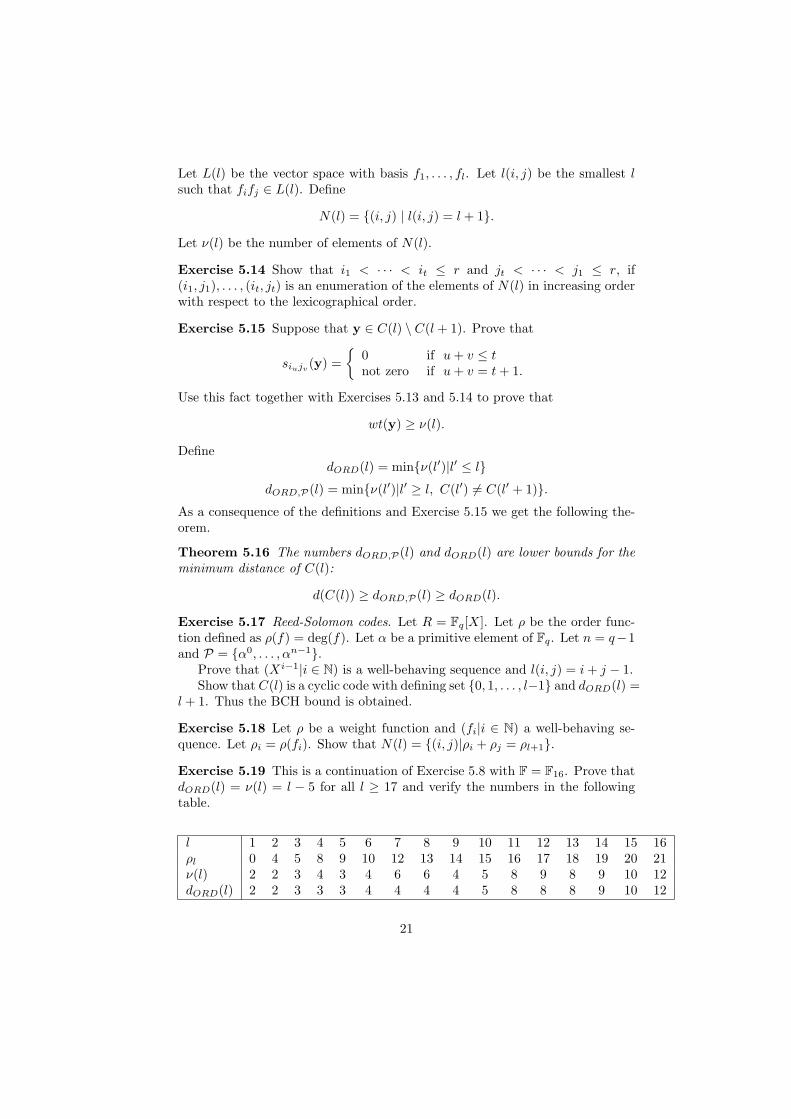
Exercise 5.19 This is a continuation of Exercise 5.8 with F = F16. Prove thatdORD(l) = ν(l) = l − 5 for all l ≥ 17 and verify the numbers in the followingtable.

l 1 2 3 4 5 6 7 8 9 10 11 12 13 14 15 16ρl 0 4 5 8 9 10 12 13 14 15 16 17 18 19 20 21ν(l) 2 2 3 4 3 4 6 6 4 5 8 9 8 9 10 12dORD(l) 2 2 3 3 3 4 4 4 4 5 8 8 8 9 10 12

21

Show that there are exactly 64 zeros of the ideal X5 + Y 4 + Y with coordinatesin F16. Denote this zero set by P. Determine dORD,P(l) for all l.

Exercise 5.20 Suppose that ρ is a weight function. Let γ be the number ofgaps. Show that dORD(l) ≥ l + 1− γ.

Exercise 5.21 Reed-Muller codes. Let R = Fq[X1, . . . , Xm] and let ρ be theorder function associated to the lexicographical total degree order on the mono-mials of R. Let n = qm. Let P = {P1, . . . , Pn} be an enumeration of the qm

points of Fmq .

Show that ν(l) =∏

(εi + 1) and dORD(l) = (∑

εi) + 1 when fl+1 =∏

Xεii .

Now suppose that fl+1 = Xr+1m . Then {fi|i ≤ l} is the set of monomials

of degree at most r. The corresponding words {hi|i ≤ l} generate RMq(r, m),the Reed-Muller code over Fq of order r in m variables. So C(l) is the dual ofRMq(r, m)which is in fact equal to RMq((q − 1)m− r − 1, r).

Write r + 1 = ρ(q − 1) + µ with ρ, µ ∈ N0 such that µ < q − 1. Prove thatd(C(l)) = dORD,P(l) = (µ + 1)qρ.

6 Notes

We use [9, 14, 15] as a reference for the theory of Grobner bases, and [33, 34]for the theory of error-correcting codes. The computer algebra packages Axiom[29], GAP [20] and Macaulay [38] are used for the computations.

The weightenumerator and MacWilliams identity is treated in [33, 34].See [16] and the project on Golay codes in this book for more about auto-

morphism groups of codes and its connection with designs.For an algorithm to compute the automorphism group of a code we refer to

[32].

For questions concerning complexity issues in coding theory we refer to [7]. Therecent proof of the NP completeness of finding the minimum distance of a linearcode is in [41]. This answers a problem posed in [11]. For cyclic codes there isan algorithm [8] to compute the weight enumerator that is much faster than themethods presented here.

See [13] for the tables of optimal q-ary codes for q = 2, 3 and 4. There isan online connection to the latest state of the table [12] which can also be usedto propose a new worldrecord. The algorithm of Brouwer is incorporated in thecoding theory package GUAVA [6, 37].

For finite geometry and projective system we refer to [27, 40].The treatment of the weight enumerator in Section 3.4 is from [30, 40] and

this way of computing the weight distribution has been implemented by [10].

The treatment of the Mattson-Solomon polynomial can be found in [33, 34].The proof of Proposition 4.7 is from [33, Chap 6] or [34, Chap 8 §6]. The proofof Proposition 4.9 is from [34, Chap 8 §6 Theorem 24]. The relation with theordinary Newton identies is explained in [34, Chap 8 §6 (52)].

22

The method in Section 4.2 to get the minimal codewords of cyclic codes isfrom [1, 2, 3, 4, 5]. This can be generalized to all linear codes as will be ex-plained in the next chapter.

Goppa [21, 22, 23, 24, 25] used algebraic curves to construct codes. These codesare called nowadays geometric Goppa codes or algebraic geometry codes, andgive asymptotically good codes, even better than the Gilbert-Varshamov bound[40]. The mathematics is quite deep and abstract. For the construction and theparameters of these codes one needs the theory of algebraic curves or algebraicfunction fields of one variable [39], in particular the Theorem of Riemann-Roch.The asymptotically good codes require the knowledge of modular curves. Sev-eral authors [17, 18, 19, 28, 31] have proposed a more elementary approach toalgebraic geometry codes and this new method has much to do with Grobnerbases [36].

The notion of order order and weight functions and its relation with codingtheory is developped in [26, 36].

Section 5 is from [28, 31, 36]. Theorem 5.9 is from [36]. The values of aorder function form a semigroup in case of a weight function. The order boundis called the Feng-Rao bound and is computed in terms of the properties of thesemigroup [31]. The way Reed-Muller codes are treated in Exercise 5.21 is from[26, 35].

A classical treatment of algebraic geometry codes is given in [39, 40].

References

[1] D. Augot, ”Description of minimum weight codewords of cyclic codes byalgebraic systems,” Un. de Sherbrooke, preprint Aug. 1994.

[2] D. Augot, ”Algebraic characterization of minimum codewords of cycliccodes,” Proc. IEEE ISIT’94, Trondheim, Norway, June 1994.

[3] D. Augot, ”Newton’s identities for minimum codewords of a family ofalternant codes,” preprint 1995.

[4] D. Augot, P. Charpin and N. Sendrier, ”Weights of some binary cycliccodewords throughout Newton’s identities,” Eurocode ’90, Springer-Verlag, Berlin 1990.

[5] D. Augot, P. Charpin and N. Sendrier, ”Studying the locator polynomialof minimum weight codewords of BCH codes,” IEEE Trans. Inform. The-ory, vol. -38, pp. 960-973, 1992.

[6] R. Baart, J. Cramwinckel and E. Roijackers, ”GUAVA, a coding theorypackage,” Delft Un. Techn., June 1994.

[7] A. Barg, ”Complexity issues in coding theory,” to appear in Handbookof Coding Theory, (V.S. Pless, W.C. Huffman and R.A. Brualdi eds.),Elsevier.

23

[8] A. Barg and I. Dumer, ”on computing the weight spectrum of cycliccodes,” IEEE Trans. Inform. Theory, vol. 38, pp. 1382-1386, 1992.

[9] T. Becker and V. Weispfenning, Grobner basis; a computational approachto commutative algebra, Springer, Berlin 1993.

[10] M. Beckker and J. Cramwinckel, ”Implementation of an algorithm for theweight distribution of block codes,” Modelleringcolloquium, EindhovenUn. Techn., Sept. 1995.

[11] E.R. Berlekamp, R.J. McEliece and H.C.A. van Tilborg, ”On the inherentintractibility of certain coding problems,” IEEE Trans. Inform. Theory,vol. -24, pp. 384-386, 1978.

[12] A.E. Brouwer, http://www.win.tue.nl/win/math.dw.voorlincod.html

[13] A.E. Brouwer and T. Verhoeff, ”An updated table of minimum-distancebounds for binary linear codes,” IEEE Trans. Inform. Theory, vol. -39,pp. 662-677, Mar. 1993.

[14] A.M. Cohen, ”Grobner bases, an introduction,” this volume.

[15] D. Cox, J. Little and D. O’Shea, Ideals, varieties and algorithms; an in-troduction to computational algebraic geometry and commutative algebra,Springer, Berlin 1992.

[16] H. Cuypers and H. Sterk, ”Working with permutation groups,” this vol-ume.

[17] G.-L. Feng and T.R.N. Rao, ”A simple approach for construction ofalgebraic-geometric codes from affine plane curves,” IEEE Trans. Inform.Theory, vol. -40, pp. 1003-1012, July 1994.

[18] G.-L. Feng and T.R.N. Rao, ”Improved geometric Goppa codes Part I,Basic Theory,” IEEE Trans. Inform. Theory, vol. -41, pp. 1678-1693, Nov.1995.

[19] G.-L. Feng, V. Wei, T.R.N. Rao and K.K. Tzeng, ”Simplified understand-ing and efficient decoding of a class of algebraic-geometric codes,” IEEETrans. Inform. Theory, vol. -40, pp. 981-1002, July 1994.

[20] GAP: Group algorithms and programming, Math. Dept. RWTH Aachen,gap-forum@math.rwth.aachen

[21] V.D. Goppa, ”Codes associated with divisors,” Probl. Peredachi Inform.vol. 13 (1), pp. 33-39, 1977. Translation: Probl. Inform. Transmission,vol. 13, pp. 22-26, 1977.

[22] V.D. Goppa, ”Codes on algebraic curves,” Dokl. Akad. Nauk SSSR, vol.259, pp. 1289-1290, 1981. Translation: Soviet Math. Dokl., vol. 24, pp.170-172, 1981.

24

[23] V.D. Goppa, ”Algebraico-geometric codes,” Izv. Akad. Nauk SSSR, vol.46, 1982. Translation: Math. USSR Izvestija, vol. 21, pp. 75-91, 1983.

[24] V.D. Goppa, ”Codes and information,” Russian Math. Surveys, vol. 39,pp. 87-141, 1984.

[25] V.D. Goppa, Geometry and codes, Mathematics and its Applications, vol.24, Kluwer Acad. Publ., Dordrecht 1991.

[26] P. Heijnen and R. Pellikaan, ”Geneneralized Hamming weights of q-aryReed-Muller codes,” to appear in IEEE Trans. Inform. Theory.

[27] J.W.P. Hirschfeld and J.A. Thas, General Galois geometries, Oxford Uni-versity Press, Oxford 1991.

[28] T. Høholdt, J.H. van Lint and R. Pellikaan, ”Algebraic geometry codes,”to appear in Handbook of Coding Theory, (V.S. Pless, W.C. Huffman andR.A. Brualdi eds.), Elsevier.

[29] R.D. Jenks and R.S. Sutor, Axiom. The scientific computation system,Springer-Verlag, New York 1992.

[30] G.L. Katsman and M.A. Tsfasman, ”Spectra of algebraic-geometriccodes,” Probl. Peredachi Inform, vol. 23 (4), pp. 19-34, 1987. Translation:Probl. Inform. Transmission, vol. 23, pp. 262-275, 1987.

[31] C. Kirfel and R. Pellikaan, ”The minimum distance of codes in an arraycoming from telescopic semigroups,” IEEE Trans. Inform. Theory, vol.41, pp. 1720-1732, Nov. 1995.

[32] J. Leon, ”Computing the automorphism groups of error-correcting codes,”IEEE Trans. Inform. Theory, vol. 28, pp. 496-511, 1982.

[33] J.H. van Lint, Introduction to coding theory, Graduate Texts in Math. 86,Springer-Verlag, Berlin 1982.

[34] F.J. MacWilliams and N.J.A. Sloane, The theory of error-correcting codes,North-Holland Math. Library vol. 16, North-Holland, Amsterdam 1977.

[35] R. Pellikaan, ”The shift bound for cyclic, Reed-Muller and geometricGoppa codes,” Proceedings AGCT-4, Luminy 1993, Walter de Gruyter,Berlin 1996, pp. 155-175.

[36] R. Pellikaan, ”On the existence of order functions,” submitted to theproceedings of the Second Shanghai Conference on Designs, Codes andFinte Geometry, 1996.

[37] J. Simonis, ”GUAVA: A computer algebra package for coding theory,”Proc Fourth Int. Workshop Algebraic Combinatorial Coding Theory, Nov-gorod, Russia, Sept. 11-17, 1994, pp. 165-166.

25

[38] Ma. Stillman, Mi. Stillman and D. Bayer, Macaulay user manual.

[39] H. Stichtenoth, Algebraic function fields and codes, Universitext, Springer-Verlag, Berlin 1993.

[40] M.A. Tsfasman and S.G. Vladut, Algebraic-geometric codes, Mathematicsand its Application vol. 58, Kluwer Acad. Publ., Dordrecht 1991.

[41] A. Vardy, ”The intractibility of computing the minimum distance of acode,” to appear in IEEE Trans. Inform. Theory.

26