Grobner bases and wavelet design¨ - New York University

Journal of Symbolic Computation 37 (2004) 227–259

www.elsevier.com/locate/jsc

Grobner bases and wavelet design

Jerome Lebruna,∗, Ivan Selesnickb

aLaboratoire I3S, CNRS/UNSA, Sophia Antipolis, FrancebDepartment of Electrical Engineering, Polytechnic University, Brooklyn, USA

Received 5 September 2000; accepted 11 June 2002

Abstract

In this paper, we detail the use of symbolic methods in order to solve some advanced designproblems arising in signal processing. Our interest lies especially in the construction of wavelet filtersfor which the usual spectral factorization approach (used for example to construct the well-knownDaubechies filters) is not applicable. In these problems, we show how the design equations can bewritten as multivariate polynomial systems of equations and accordingly how Gröbner algorithmsoffer an effective way to obtain solutions in some of these cases.© 2003 Elsevier Ltd. All rights reserved.

Keywords:Discrete wavelet transform (DWT); Conjugate quadrature filters (CQFS)

0. Introduction

Wavelets and filter banks have become useful in digital signal processing in part becauseof their ability to represent piecewise smooth signals with relative efficiency. For suchsignals, the discrete wavelet transform (DWT) of ann-point vector is again ann-pointvector, but one for which the energy is compacted into fewer values. In as far as this istrue, the DWT is useful for signal compression (JPEG 2000), fast algorithms, and signalestimation and modeling (noise suppression and image segmentation, etc). The DWT isusually implemented as an iterated digital filter bank tree, so the design of a wavelettransform amounts to the design of a filter bank.

While the spectral factorization approach is the most convenient method to constructthe classic wavelets (Daubechies, 1992) (and the corresponding digital filters), it is not

∗ Corresponding author.E-mail addresses:[email protected] (J. Lebrun), [email protected] (I. Selesnick).URLs:http://www.i3s.unice.fr/∼lebrun, http://www.taco.poly.edu/selesi.

0747-7171/$ - see front matter © 2003 Elsevier Ltd. All rights reserved.doi:10.1016/j.jsc.2002.06.002

http://www.i3s.unice.fr/~lebrun

http://www.taco.poly.edu/selesi

http://www.elsevier.com/locate/jsc

228 J. Lebrun, I. Selesnick / Journal of Symbolic Computation 37 (2004) 227–259

applicable to many of the other wavelet design problems where additional constraints areimposed. However, for many of these design problems, the design equations can be writtenas a multivariate polynomial system of equations. Accordingly, Gröbner basis algorithmsoffer a way to obtain solutions in these cases. This paper describes the general waveletdesign problem from the perspective of filter banks and explains the derivation of the coredesign equations. In addition, it is noted that the design of wavelet bases is intriguing inpart for its limitations—specifically, in many cases it is not possible to obtain waveletshaving all the properties one desires. This has motivated the development, for example, ofmultiwavelet bases, which are developed inSections 5and6, and of wavelet frames (ofovercompletebases) which are described inSection 7. For both multiwavelet bases andsome wavelet frames, the spectral factorization approach which is key in the constructionof Daubechies wavelets, cannot be used anymore. However, as described in the followingrespective sections, it becomes possible to derive solutions to these new problems usingGrobner bases.

Recently, major advances have been achieved in the field of computational algebraicgeometry that lead to new efficient ways to deal with one of the central applications ofcomputer algebra: solving systems of multivariate polynomial equations. Using the newalgorithms that have been developed, practical problems like (multi)wavelet design cannow be solved exactly in a way that is very competitive with numerical methods. One of themost promising schemes to solve systems of polynomial equations has been by computingGrobner bases. At the same time, even though the computation of a Gröbner basis is thecrucial point in our approach, one should not forget that it is only the first step in the solvingprocess. Methods to implement change of ordering of the Gröbner basis, and alternativeapproaches like triangular systems and rational univariate representation of the systemare also key tools. We will discuss some of these methods in the following. For previousapplications of Gröbner bases to the design of wavelets and digital filters, see for examplethe works ofPark et al.(1997), Faugere et al.(1998), Lebrun(2000), Lebrun and Vetterli(2001), Selesnick and Burrus(1998), Selesnick(1999) andSelesnick(2000b).

Following a filter bank perspective, we introduce filter banks based on conjugatequadrature filters (CQFs), and we give a simple introduction to wavelets. Iteration of thefilter bank on the lowpass analysis generates discrete-time wavelet bases. In the limit, weend up with wavelet bases and the concept of multiresolution analysis. We also highlightthe motivation for introducing multiwavelets as a way to overcome some limitationsof CQFs. Readers interested in a more detailed presentation of filter bank and wavelettheory are referred to the classical books ofDaubechies(1992), Vaidyanathan(1993),Vetterli and Kovaˇcevic (1995), Strang and Nguyen(1996), Burrus et al.(1998) andMallat(1998).

1. Preliminaries

The Z-transform of a discrete-time signal, defined as

X(z) = Z{x(n)} =∑

n

x(n)z−n

J. Lebrun, I. Selesnick / Journal of Symbolic Computation 37 (2004) 227–259 229

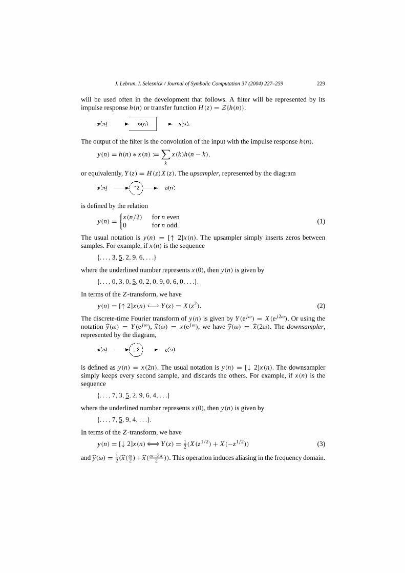
will be used often in the development that follows. A filter will be represented by itsimpulse responseh(n) or transfer functionH (z) = Z{h(n)}.

The output of the filter is the convolution of the input with the impulse responseh(n).

y(n) = h(n) ∗ x(n) :=∑

k

x(k)h(n− k),

or equivalently,Y(z) = H (z)X(z). Theupsampler, represented by the diagram

is defined by the relation

y(n) ={

x(n/2) for n even0 for n odd.

(1)

The usual notation isy(n) = [↑ 2]x(n). The upsampler simply inserts zeros betweensamples. For example, ifx(n) is the sequence

{. . . ,3,5,2,9,6, . . .}where the underlined number representsx(0), theny(n) is given by

{. . . ,0,3,0,5,0,2,0,9,0,6,0, . . .}.In terms of theZ-transform, we have

y(n) = [↑ 2]x(n) Y(z) = X(z2). (2)

The discrete-time Fourier transform ofy(n) is given byY(ejω) = X(ej 2ω). Or using thenotation y(ω) = Y(ejω), x(ω) = x(ejω), we havey(ω) = x(2ω). The downsampler,represented by the diagram,

is defined asy(n) = x(2n). The usual notation isy(n) = [↓ 2]x(n). The downsamplersimply keeps every second sample, and discards the others. For example, ifx(n) is thesequence

{. . . ,7,3,5,2,9,6,4, . . .}where the underlined number representsx(0), theny(n) is given by

{. . . ,7,5,9,4, . . .}.In terms of theZ-transform, we have

y(n) = [↓ 2]x(n) Y(z) = 12(X(z

1/2)+ X(−z1/2)) (3)

andy(ω) = 12 (x(

ω2 )+ x(ω−2π

2 )). This operation induces aliasing in the frequency domain.


1.1. Filter banks

The basic principle of filter banks is to decompose signals into lowpass and highpasscomponents at half the rate of the input signal (so as to keep the same amount of data) insuch a way that it is possible to exactly reconstruct the input signal from these components.This subject of interest,subband coding with multirate filter banks, became an activetopic whenCroisier et al.(1976) showed it was possible to construct filter banks withaliasing cancellation using quadrature mirror filters (QMF) and simple downsampling andupsampling operations.

An analysis filter bank decomposes a signalx0 into two subband signalsx1 andd1 asshown in the diagram.

Consequently, a two-channel multirate filter bank first convolves the input signalx0 with alowpass filterg0 and a highpass filterg1 to minimize aliasing and then downsamples thesetwo signals.

x1 = [↓ 2](g0 ∗ x0) and d1 = [↓ 2](g1 ∗ x0). (4)

Explicitly, we have

x1(n) =∑

k

x0(k)g0(2n− k) and d1(n) =∑

k

x0(k)g1(2n− k). (5)

A synthesis filter bank combines the subband signals into a single signal.

The output signal is then reconstructed by upsamplingx1 andd1 and filtering again witha lowpass filterh0 and a highpass filterh1 to reject the out-of-band components in thespectrum. The synthesis is given by

y0 = h0 ∗ ([↑ 2]x1)+ h1 ∗ ([↑ 2]d1). (6)

Explicitly, we have

y0(n) =∑

k

x1(k)h0(n− 2k)+∑

k

d1(k)h1(n− 2k). (7)

A perfect reconstruction (PR) filter bank is one where the synthesis filter bank perfectlyreconstructs the inputx0 from the subband signalsx1 andd1; that is, one wherey0 = x0.


For a PR filter bank, the synthesis filtersh0, h1 together with their translates by evenintegers form a basis forl 2(Z) and (7) can be written as

x0(n) =∑

k

〈x0, h0,k〉h0,k(n)+∑

k

〈x0, h1,k〉h1,k(n) (8)

where

hi,k(n) = hi (n− 2k) and hi,k(n) = gi (2k− n) for i = 0,1. (9)

The dual basis{hi,k} is comprised of the reversed versions of the analysis filtergi (n) andtheir translates by even integers.

Vetterli gave the necessary and sufficient conditions in thez-domain for PR (in factgeneralized PR, since delays of the formz−l are allowed):

G0(z)H0(z)+ G1(z)H1(z) = 2z−l (10)

G0(z)H0(−z)+ G1(z)H1(−z) = 0. (11)

For filters satisfying these PR conditions, the signalx0 can be recovered fromx1 andd1.In this case the subband signals provide an alternate representation of the input signalx0. The goal is to design the four filters such that the filter bank is PR and such thatthe new representation ofx0 is more efficient and thus facilitates signal processing tasks.Although the PR conditions do not demand it, applications of the subband decomposition(Crochiere et al., 1976) generally call for the filtersh0 andg0 to be lowpass, and the filtersh1 andg1 to be highpass so thatx1 andd1 have more or less disjoint spectrums.

From the PR conditions, we get thatg0 andg1 are uniquely determined fromh0 andh1

by rewriting the previous equations[H0(z) H1(z)

H0(−z) H1(−z)

] [G0(z)G1(z)

]=[

2z−l

0

]. (12)

IntroducingD(z) := H0(z)H1(−z) − H0(−z)H1(z), supposed to be non-vanishing onT,we get

G0(z) = 2z−l

D(z)H1(−z) and G1(z) = − 2z−l

D(z)H0(−z). (13)

Now, if we require further that all filters have finite impulse response (FIR, i.e. a finitenumber of taps), then essentially only two choices are possible forD(z) andz−l . Namely,

Quadrature mirror (QMF). D(z) = 2z−l .This gives G0(z) = H1(−z) and G1(z) = −H0(−z). Now, Croisier et al. (1976)additionally imposedh0 andh1 to be mirror filters (H1(z) := H0(−z)), we then get

H 20 (z)− H 2

0 (−z) = 2z−l (14)

where l is necessarily odd. The solutions of this equation are naturally called QMF.Unfortunately, the only solutions being FIR QMF are variations of the Haar filterH0(z) =1/√

2(1+ z−1). The interest of these filters is rather limited.


Conjugated quadrature filters (CQF). D(z) = 2z−l−1.We get G0(z) = zH1(−z) and G1(z) = −zH0(−z). Smith and Barnwell(1984) andMintzer (1985) were able to overcome the major limitation of QMF by imposingh0 andh1 to be CQFs:H1(z) := −z−1H0(−z−1). We get

H0(z)H0(z−1)+ H0(−z)H0(−z−1) = 2z−l , (15)

wherel is necessarily even. With this slight change, FIR solutions are now possible. Andas we will see, these filters are closely linked to wavelets.

1.2. Zero moments

The filter bank provides an efficient representation of piece-wise smooth signals if thesubband signald1 is close to zero for smooth signalsx0 and if the filterh1 is short. That is,for signal compression, we wantd1 ≈ 0 wheneverx0 is smooth. As a vehicle for achievingthis, it is common to ask thatd1 = 0 wheneverx0 is a discrete-time polynomial of specifieddegree.

It can be shown that the filterG1(z) annihilates polynomial signals of degreeK − 1 ifand only if(z− 1)K dividesG1(z), or equivalently, if∑

n

nk(−1)ng1(n) = 0, for 0≤ k ≤ K − 1.

That is, the filterg1 hasK zero moments.

1.3. Orthonormal filter banks

If the analysis filtersg0, g1 of a PR filter bank are related to synthesis filterh0, h1 by atime-reversal,

g0(n) = h0(−n), g1(n) = h1(−n),

or equivalently

G0(z) = H0(z−1), G1(z) = H1(z

−1),

then the filter bank is said to be anorthonormal filter bank. Orthonormal filter banks havedesirable statistical properties. In this case, the PR conditions become

H0(z)H0(z−1)+ H1(z)H1(z

−1) = 2 (16)

H0(−z)H0(z−1)+ H1(−z)H1(z

−1) = 0. (17)

It is easily verified that settingh1 to the CQF filter ofh0, i.e. h1(n) = (−1)nh0(1− n)or equivalentlyH1(z) = z−1H0(−z−1), it supplies a solution to the second of the two PRconditions. With this form forH1(z), the first PR condition becomes

H0(z)H0(z−1)+ H0(−z)H0(−z−1) = 2, (18)

or equivalently∑n

h0(n)h0(n− 2k) = 2δ(k) ={

2 k = 00 k �= 0.


For an orthonormal filter bank, all the filters are determined byH0(z):

H1(z) := −z−1H0(−z−1), G0(z) = H0(z−1), G1(z) = zH0(−z).

Moreover, the decomposition of a signalx0 by an orthonormal filter bank may beinterpreted as its expansion in an orthonormal basis of2. Namely the expansion (8)is an orthonormal one. This result can be generalized to IIR (non-FIR) filter banks.Besides, if the filters are not imposed to be CQF then we get biorthogonal bases of2

(Vetterli and Herley, 1992).Note that if(z− 1)K dividesG1(z), thenG1(1) = 0, and so for an orthonormal filter

bank we haveH0(−1) = 0. Substitutingz= 1 in (18) gives

H 20 (1) = 2. (19)

Furthermore, if(z−1)K dividesG1(z), then(z+1)K dividesH0(z). Daubechies’ problemis the following. GivenK , find H (z) of minimal degree such that

1.∑

n h(n)h(n− 2k) = 2δ(k)

2. (z+ 1)K dividesH (z).

It turns out that the solutionsh(n) of minimal degree can be most conveniently found bydefining a product filterP(z). Letting P(z) := H (z)H (z−1), we have the requirement thatP(z) + P(−z) = 2. Hence, orthonormal filter banks can be obtained by designingP(z)satisfying thislinear condition. BecauseP(ejω) = |H (ejω)|2, P(z) must be non-negativefor all z = ejω, otherwise it does not admit the factorizationP(z) = H (z)H (z−1). Alsonote that if(z+ 1)K dividesH (z), then(z+ 1)2K dividesP(z).

Gathering these conditions together gives an alternate form of Daubechies’ designproblem: givenK , find P(z) of minimal degree such that

1. P(ejω) ≥ 0 for allω

2. P(z) = P(z−1)

3. P(z)+ P(−z) = 2

4. (z+ 1)2K dividesP(z).

The solution is given by

P(z) = 2(1− y)KK−1∑k=0

(K + k − 1

k

)yk (20)

wherez= ejω andy = 1/2(1− cosω).The key to this solution is (1) that all constraints onH (z) can be converted into linear

constraints onP(z), and (2) thatH (z) can be obtained fromP(z) by the Fejer–Riesztheorem and spectral factorization. For other design problems where additional constraintsare imposed, it is not possible to convert the constraints onH (z) into linear constraintson P(z). It is in those cases that Gröbner bases can be used to investigate the existence ofsolutions having various desired properties.


2. Daubechies solution

To illustrate the Gröbner basis-design of orthonormal filter banks we begin by showingan example of the design of Daubechies filters of length 8. Although they can be obtainedthrough simpler means, it is a good example with which to begin.

Let R(z) be the remainder obtained after dividingH (z) by (z + 1)K . Then therequirement that(z + 1)K divides H (z) can be written asR(z) = 0. To simplify thenotation, we denoteh(n) by hn. WhenK = 4, the minimal lengthh(n) that satisfies theorthonormality condition is of length 8 (the degree ofH (z) is 7). ForK = 4, length 8, thedesign equations forh(n) are:

// Orthonormality conditions

h20 + h2

1+ h22+ h2

3 + h24+ h2

5 + h26+ h2

7− 2= 0

h7h5 + h6h4+ h2h0 + h3h1+ h4h2+ h5h3 = 0

h6h2 + h7h3+ h4h0 + h5h1 = 0

h6h0 + h7h1 = 0.

// Zero-moment conditions

h0 − h4+ 20h7− 10h6+ 4h5 = 0

h1 + 15h5+ 70h7− 36h6− 4h4 = 0

h2 − 45h6+ 84h7+ 20h5− 6h4 = 0

h3 + 35h7− 20h6+ 10h5− 4h4 = 0.

Note that the first condition∑

n h2n = 2 is the only non-homogeneous equation. We can

replace it by the equationH 2(1) = 2 without affecting the set of solutions. In addition,the negation of each solution vector is also a solution (ifhn is a solution, then so is−hn).Therefore, we can reduce the number of solutions by replacing the constraintH 2(1) = 2with the constraintH (1) = +√2. To simplify the Grobner basis calculations, we canreplace the equationH (1) = +√2 by H (1) = 1, then the equations are in terms ofrationals only. This has the effect only of scaling all solution vectors by 1/

√2. The solution

can be rescaled afterwards to obtain the correct normalization. This procedure reduces thedegree of the set of equations by a factor of two.

If the first equation above is replaced by the equation

h0 + h1+ h2+ h3 + h4+ h5 + h6+ h7− 1= 0

then lexicographic Gröbner basis is


h(n)

–0.5

0

0.5

1

–0.5

0

0.5

1

–0.5

0

0.5

1

–0.5

0

0.5

1

0

0.5

1

1.5

0

0.5

1

1.5

0

0.5

1

1.5

0

0.5

1

1.5

|H(ejω)|

0 2 4 6 8 0 0.2 0.4 0.6 0.8 1

0 2 4 6 8 0 0.2 0.4 0.6 0.8 1

0 2 4 6 8 0 0.2 0.4 0.6 0.8 1

0 2 4 6 8 0 0.2 0.4 0.6 0.8 1

Fig. 1. The 4 orthonormal filters of length 8 with 4 zero moments.

Appending the following equation

h1 + 2h2+ 3h3+ 4h4+ 5h5+ 6h6+ 7h7− A (21)

yields a more compact Gröbner basis:

4A8 − 112A7 + 1344A6 − 9016A5 + 36904A4 − 94080A3 + 145096A2 − 122500A+ 423854480h7 − 16A7 + 392A6 − 4004A5 + 22050A4 − 70476A3 + 130074A2 − 126910A+ 489654480h6 − 16A7 + 392A6 − 4004A5 + 22050A4 − 70476A3 + 129934A2 − 126210A+ 482654480h5 + 48A7 − 1176A6 + 12012A5 − 66150A4 + 211428A3 − 390502A2 + 381850A− 1477354480h4 + 48A7 − 1176A6 + 12012A5 − 66150A4 + 211428A3 − 390082A2 + 379190A− 1447954480h3 − 48A7 + 1176A6 − 12012A5 + 66150A4 − 211428A3 + 390782A2 − 384090A+ 1496954480h2 − 48A7 + 1176A6 − 12012A5 + 66150A4 − 211428A3 + 390362A2 − 380870A+ 1447954480h1 + 16A7 − 392A6 + 4004A5 − 22050A4 + 70476A3 − 130354A2 + 129150A− 531654480h0 + 16A7 − 392A6 + 4004A5 − 22050A4 + 70476A3 − 130214A2 + 127890A− 50505.

The lexicographic Gröbner basis can be obtained from the degree-Gröbner basis using theFGLM algorithm, as described below in the Appendix.

Of the eight solutions, four are real-valued, four are complex-valued. The four real-valued solutions are shown inFig. 1. Notice that the reverse of each solution is also asolution. Not counting negation and reversal, there are two distinct solutions.

As noted above, the Daubechies filters can be obtained via the spectral factorizationof a suitably designed (Laurent) polynomialP(z), as described by Daubechies. In thisprocedure, Gröbner bases are not required, as the design ofP(z) is a linear problem and


spectral factorization requires finding the roots of a univariate polynomial only. However,if it is desired that the filterh(n) satisfy additional constraints, it is likely that the spectralfactorization approach cannot be used. For example, if it is desired thath(n) be nearlysymmetrich(no − n) ≈ h(n) then the design problem becomes more complicated andGrobner bases can be utilized. (For image processing, it is desirable that a filter bank consistof symmetric filters because the distortion introduced by filtering with non-symmetricfilters is sometimes visible.) It is well-known that exactly symmetric finite-length solutionsdo not exist for the orthonormal two-channel filter bank design problem, for the exceptionof the Haar solution withH (z) = 1√

2(1+ z−1).

For this reason, it is common to use (1) orthonormal PR filter banks with nearlysymmetric filters or (2) symmetric PR filter banks that are nearly orthonormal. Whilethe design of these types of filter banks can be approximately carried out by differentfactorizations ofP(z) in (20), many algorithms have been suggested for these two classesthat designh(n) directly rather thanp(n).

The design of nearly symmetric orthonormal PR filter banks is described in the nextsection, where Gröbner bases are used to obtain the filters. An alternative is to usemultiwavelets, for which orthonormality and symmetry are simultaneously possible. Thedesign of multiwavelets is detailed inSections 5and6.

3. Nearly symmetric orthonormal filter bank

While the classic Daubechies filters can be obtained without having to solve anymultivariate nonlinear equations, many generalizations and specialized designs that satisfyadditional constraints cannot be obtained so easily. As an example, consider the design of alength 8 filterh(n) satisfying the orthonormality condition (18), with some zero momentsand some degree of symmetry (Abdelnour and Selesnick, 2001). To enforce a degree ofsymmetry, we ask that

h(no + n) = h(no − n)

for some selected range ofn. If there were no symmetry constraints, then the filter bankcould have at most four zero moments. Because of the symmetry constraints, the filter bankwill have fewer zero moments. TakingK = 2, no = 2.5, we can get the following designproblem. DesignH (z) of minimal degree such that,

1. h(2) = h(3), h(1) = h(4).2. (z+ 1)2 dividesH (z).3.∑

n hnhn−2k = δ(k).This design problem gives rise to the following design equations.

// Orthonormality conditions

h0 + h1+ h2+ h3 + h4+ h5 + h6+ h7− 1

h2h0 + h3h1+ h4h2 + h5h3+ h6h4+ h7h5

h6h2 + h4h0+ h5h1 + h7h3

h6h0 + h7h1.


// Zero-moment conditions

h0 − h2− 3h4− 5h6+ 6h7+ 4h5+ 2h3

h1 + 3h3+ 5h5+ 7h7− 6h6− 4h4− 2h2.

// Partial symmetry conditions

h2 − h3

h1 − h4.

As above, appending Eq. (21) has the effect of simplifying the coefficients appearingin the Grobner basis. It turns out that the lexicographic Gröbner basis then factors intotwo parts. We used thefacstd command inSingular(Greuel et al., 2000) to perform thefactorization. The first Gröbner basis is

40A6− 984A5+ 9796A4− 49888A3+ 135314A2− 183246A+ 95445,

106688h7+ 800A5− 18060A4+ 156848A3− 646136A2+ 1231488A− 828755,

320064h6− 800A5+ 18060A4− 156848A3+ 646136A2− 1284832A+ 962115,

26672h5− 400A5+ 9030A4− 78424A3+ 321401A2− 607409A+ 405209,

32h4− 2A2+ 18A− 35,

106688h3+ 800A5− 18060A4+ 156848A3− 632800A2+ 1138136A− 728735,

106688h2+ 800A5− 18060A4+ 156848A3− 632800A2+ 1138136A− 728735,

32h1− 2A2+ 18A− 35,

80016h0− 400A5+ 9030A4− 78424A3+ 318067A2− 577403A+ 353532.

The second Gröbner basis is

2A2− 18A+ 33,

16h7− 2A+ 5,

16h6− 2A+ 5,

16h5+ 1,

16h4− 1,

16h3+ 2A− 13,

16h2+ 2A− 13,

16h1− 1,

16h0+ 1.

The first part has four real-valued solutions and two complex-valued solutions. Thesecond part has two real-valued solutions. The six real solutions are shown inFig. 2. Thefrequency responses|H (ejω)| are also shown in the figure. Only the last solution is areasonable lowpass filter. The other five solutions can be considered parasitic solutions.They would not be favored in practice because they do not have acceptable lowpassfrequency responses.


0 2 4 6 8 0 0.2 0.4 0.6 0.8 1

0 2 4 6 8 0 0.2 0.4 0.6 0.8 1

0 2 4 6 8 0 0.2 0.4 0.6 0.8 1

0 2 4 6 8 0 0.2 0.4 0.6 0.8 1

–0.5

0

0.5

1

0

0.5

1

1.5

0

0.5

1

1.5

0

0.5

1

1.5

0

0.5

1

1.5

0

0.5

1

1.5

0

0.5

1

1.5

–0.5

0

0.5

1

–0.5

0

0.5

1

–0.5

0

0.5

1

–0.5

0

0.5

1

–0.5

0

0.5

1

0 2 4 6 8 0 0.2 0.4 0.6 0.8 1

0 2 4 6 8 0 0.2 0.4 0.6 0.8 1

h(n) |H(ejω)|

Fig. 2. The 6 orthonormal filters of length 8 with 2 zero moments and partial symmetry aboutn0 = 2.5.

It is seen in the figure, that the sixth solution, while not exactly symmetric, ismore symmetric than the solutions shown inFig. 1. Furthermore, the solution has moresymmetry than requested in the design problem; we haveh(0) = h(5) as well.

Other formulations of the nearly symmetric orthonormal filter bank design problem arebased on moments ofh(n), and the corresponding wavelets are calledCoiflets(Daubechies,1992; Tian et al., 1997; Wei and Bovik, 1998). The design of Coiflets also requires thesolution to nonlinear design equations and usually the solutions are found through iterativenumerical optimization. As detailed inSection 6.2, Grobner bases can also be used toobtain Coiflets (in fact multiCoiflets).


4. Iterated filter banks

The filter bank structure described above is often used in an iterated manner. Indeed,the analysis of a signal over several scales (multiresolution analysis) can be accomplishedby iterating the filter bank on the first subband. The idea of filter bank trees is to cascadethis iteration up to a certain levell . We then havel + 1 signals: the coarse signalxl and thedetails signalsdl , . . . ,d1.

The original signalx0 can be reconstructed from these subband signals by the iteratedsynthesis filter bank.

If (z−1)K dividesG1(z), then not only isd1 = 0 wheneverx0 is a polynomial signal ofdegree less thanK , butd2 = 0 andd3 = 0 also. This is clarified as follows. LetPK denotethe set of discrete-time polynomials of degreeK and less; then we can write the following.If

1. x0(n) ∈ PK−1, and2. (z− 1)K dividesG1(z)

then

1. x1(n) ∈ PK−1, and2. d1(n) = 0.

Note that polynomial signals are preserved; ifx0 is a polynomial signal, then so isx1.Therefore, if G1(z) annihilates polynomials of a specified degreeK , then all of thesubbandsdi are zero whenever the input is a polynomial of the same degree.

Now, if we omit some detail signals,di (n), in the reconstruction (this is the principleof compression), the “quality” of the signal reconstructed will depend largely on the


“smoothness” (Mallat, 1989; Daubechies, 1992; Rioul, 1993) of the basis vectors withwhich the reconstruction is performed.

4.1. Wavelet bases

The transformation of a signalx0 by anl -level iterated filter bank into subband signalsd1,d2, . . . ,dl , xl constitutes the DWT. A wavelet basis forL2(R) is closely related tothe DWT. In particular, given an orthonormal DWT (fully determined byh0(n)), anorthonormal wavelet basis forL2(R) is given by

{φ(t − k), 2 j /2ψ(2 j t − k) : j , k ∈ Z, j ≥ 0}where the scaling functionφ(t) is defined through the dilation equation (or two-scalerelation):

φ(t) = √2∑

n

h0(n)φ(2t − n)

and the wavelet is defined by

ψ(t) := √2∑

n

h1(n)φ(2t − n).

Furthermore, if(z+ 1)K dividesH0(z) then∫tkψ(t) dt = 0 for 0≤ k ≤ K − 1

and ∑n

nkφ(t − k) ∈ Pk.

Therefore, the design of an orthonormal wavelet basis forL2(R) is equivalent to thedesign of an orthonormal filter bank. Implementation is nearly always performed usingfilter banks, but the functionsφ(t) andψ(t) are useful because they indicate how thefilter bank behaves when the filter bank is iterated indefinitely. For example, if the filterbank is not designed so that(z + 1)2 divides H0(z), thenφ(t) will not be continuous.The smoothness ofφ(t) is important because it reflects what artifacts may appear in thesynthesized signaly(n).

The scaling functionsφ(t) for the examples above are shown inFigs. 3and4, fromwhich the comparative symmetry of the second problem is also visible.

It should be noted that a solution (in theL2 sense) to the dilation equation (a scalingfunction) does not always exist. However, if inf|ω|<π3

|h0(ω)| > 0, then the convergence

is in L2 norm (Cohen, 1992) to a bona-fideL2 function. In that case, these two functionsgenerate a multiresolution analysis ofL2 as defined byMallat (1989). Defining Vk :=span{φ(2−kt − n) | n ∈ Z}, we get by the two-scale equations, a nested sequence ofsubspaces ofL2 satisfying

• Vn ⊂ Vn−1.• ∩nVn = {0} and∪nVn = L2.


–0.5

0

0.5

1

1.5

–0.5

0

0.5

1

1.5

0 2 4 6

0 2 4 6

Fig. 3. The scaling functions generated by the first two filters shown inFig. 1.

–0.5

0

0.5

1

1.5

0 2 4 6

Fig. 4. The scaling function generated by the sixth filter shown inFig. 2.

• f ∈ Vn ⇔ f (2t) ∈ Vn−1.• f ∈ V0⇔ f (t − k) ∈ V0, ∀k ∈ Z.• {φ(t − k) | k ∈ Z} is an orthonormal basis ofV0.

IntroducingWk := span{ψ(2−kt − n) | n ∈ Z}, we getVn−1 = Vn ⊕ Wn and so⊕nWn = L2. It is easily proven that{ψ(2kt − n) | k,n ∈ Z} is an orthonormal basisof L2. Starting from a CQF, we have constructed a basis ofL2 from dyadic dilationsand translations of a single function.ψ is called an orthonormal wavelet,φ is called theassociated scaling function. Again, thequality of the multiresolution analysis is measuredby the numberK of zeros atπ of H0(ejω) since it implies that 1, t, . . . , t K−1 can be exactlyreconstructed from integer translates of the scaling function, thus giving approximationorderK (Jia and Lei, 1993).

This way of constructing wavelets from iterated filter banks was pioneered byDaubechies(1988). It became since, a standard way to derive orthonormal and bi-orthogonal wavelet bases. The underlying CQF filter banks are now well-studied, thedesign procedure is well-understood. By the structure of the problem, certain solutionsare however ruled out: since it is impossible to design FIR linear-phase CQF with realcoefficients other than the Haar filter, this implies that the only orthonormal wavelet withcompact support and symmetry is the Haar wavelet.

For multiwavelets, however, the relation betweenφ(t),ψ(t) and the corresponding filterbank is more complicated. In the next section, the design of multiwavelets is consideredin detail. It turns out that Gröbner bases are very useful in investigating the existence ofmultiwavelets having properties that are not possible in the scalar-wavelet framework.


5. Multiwavelets

Generalizing the wavelet case, one can allow a multiresolution analysis{Vn}n∈Zof L2(R) to be generated by a finite orthonormal set of scaling functionsφ0(t),φ1(t), . . . , φr−1(t) and their integer translates. In this framework, the so-calledmultiscaling functionφ(t) := [φ0(t), . . . , φr−1(t)]� satisfies now a matrix two-scaleequation

φ(t) =∑

k

M(k)φ(2t − k) (22)

where now{M(k)}k is a sequence ofr ×r matrices of real coefficients. The multiresolutionanalysis structure givesV−1 = V0 ⊕ W0 whereW0 is the orthogonal complement ofV0 in V−1. Again, starting from the orthonormal basis,φ0(t), φ1(t), . . . , φr−1(t) andtheir integer translates, we can construct an orthonormal basis ofW0 generated byψ0(t), ψ1(t), . . . , ψr−1(t) and their integer translates with the so-called multiwaveletψ(t) := [ψ0(t), . . . , ψr−1(t)]� derived by

ψ(t) :=∑

k

N(k)φ(2t − k) (23)

where{N(k)}k is a sequence ofr × r matrices of real coefficients obtained by orthonormalcompletion(Lawton et al., 1996) of {M(k)}k. Introducing in thez-domain, the refinementmasksM(z) := 1/2

∑n M(n)z−n and N(z) := 1/2

∑n N(n)z−n, Eqs. (22) and (23)

translate in Fourier domain into

φ(2ω) =M(ejω)φ(ω) and ψ(2ω) = N(ejω)φ(ω). (24)

Under some natural conditions of convergence (detailed inCohen et al.(1997) andLebrun(2000)), and similarly to the wavelet case, we can derive the behavior of the multiscalingfunction by iterating the first product above. We get at the limit

φ(ω) =M∞(ω)φ(0) =∞∏

i=1

M(ejω/2i)φ(0). (25)

In the sequel, we will impose that the sequences{M(k)}k and {N(k)}k have finitesupport and thus thatφ(t) andψ(t) have compact support (Massopust et al., 1996). Theorthonormality of the multiscaling function translates also into a matrix orthonormalitycondition onM(z): for all z on the unit circle,

M(z)M�(z−1)+M(−z)M�(−z−1) = I. (26)

With this approach, one is finally able to overcome some of the limitations ofCQF filter banks. It is now possible to get finitely generated multiresolution analysiswith all the scaling functions and wavelets being orthogonal, compactly supported and(anti)symmetric.

The first multiwavelets were designed byAlpert (1993) using methods fromnumerical analysis (finite elements and splines methods). A construction using fractalinterpolation of a multiresolution analysis having approximation order 2 (1 andt can bereconstructed from the translates of the scaling functions) using two symmetric, compactly


supported, orthogonal scaling functions (that are furthermore Lipschitz) byGeronimo et al.(1994) (DGHM) triggered many other attempts to construct new multiwavelet bases(Vetterli and Strang, 1994; Strang and Strela, 1995; Donovan et al., 1996; Chui and Lian,1996) and motivated a thorough study of the theory of multiwavelets (Heil et al., 1996;Cohen et al., 1997; Plonka, 1997; Plonka and Strela, 1998).

Considering a finitely generated multiresolution analysis with orthonormal multiscalingfunction φ(t) and multiwaveletψ(t), from V0 = V1 ⊕ W1, we get for s(t) =∑

n s�0 (n)φ(t − n) ∈ V0,

s(t) =∑

n

s�1 (n)φ(

t

2− n

)+ d�1 (n)ψ

(t

2− n

). (27)

Hence, we derive the well-knownMallat (1989) algorithm for multiwavelets. At theanalysis,

s1(n) =∑

k

M(k− 2n)s0(k) and d1(n) =∑

k

N(k − 2n)s0(k) (28)

and at the synthesis, we get

s0(n) =∑

k

M�(n− 2k)s1(k)+ N�(n− 2k)d1(k). (29)

These relations enable us to construct a multi-input multi-output filter bank (multifilterbank) as shown below.

Because of their inherent vector nature, in order to process scalar signal, multifilter banksrequire a vectorization of the input signal to produce anr -dimensional input signal.A simple way to do this vectorization is to split scalar signals into their polyphasecomponents. Introducing

m0(z)m1(z)...

mr−1(z)

:= 2M(zr )

1

z−1

...

z−(r−1)

(30)

and in the same wayn0(z),n1(z), . . . ,nr−1(z), the system can then be rewritten as a2r channel time-varying filter bank as shown inFig. 5. Intuitively, this is a filter bankwith relaxed requirements on the time invariance. In each filtering block, we periodicallyalternate between different filters.Lebrun and Vetterli(1998) andSelesnick(1998) pointedout that if the componentsm0(z),m1(z), . . . ,mr−1(z) of the lowpass branch have differentspectral behavior, e.g. lowpass behavior for one, highpass for another, this will lead tounbalanced channels that will mix the coarse resolution signal and detail coefficients and


↑4↑ 2

↑4

↑4

↑4

↑2

↑2

↑2

↑2

x1,k

x0,k x0,k

d1,k

Analysis Synthesis

↑ 2

↑ 2

↑ 2

↑ 4

↑ 4

↑ 4

↑ 4

m0(z–1)

m1(z–1)

n0(z–1)

n1(z–1)

m0(z)

m1(z)

n0(z)

n1(z)

z

z

z–1

z–1

Fig. 5. Multifilter bank seen as a time-varying filter bank.

will create strong oscillations in the reconstructed signal. This leads us to introduce theconcept of balanced multiwavelets.

5.1. Balancing

This problem relates also to the basic principle of filter banks: one expects a reasonableclass of smooth signals (typically piecewise polynomial signals) to be preserved by thelowpass branch and annihilated by the highpass one. In the wavelet case, the two importantissues of the reproduction of polynomials by the associated multiresolution analysis(approximation theory issue) and the preservation/cancellation of discrete-time polynomialsignals by the associated filter bank (subband coding and compression issue) are tightlyconnected since they have been proved to be equivalent to the Strang-Fix conditions:the number of zeros atπ in the factorization of the lowpass filterH0(ejω) of the filterbank. This is however not the case anymore for multiwavelets (Lebrun and Vetterli, 1998).The preservation/annihilation of constant signals by the lowpass/highpass branches of themultifilters (calledbalancingof order 1) is proved to be equivalent (Lebrun and Vetterli,1998; Selesnick, 1998) to any of the following conditions:

• [1,1, . . . ,1] is a left eigenvector ofM(1) with eigenvalueλ0(1) = 1.

• φ(0) = [1,1, . . . ,1]�.

• ∑r−1i=0 mi (z) has zeros on the unit circle atz= ej kπ/r for k = 1, . . . ,2r − 1.

• One can factorizeM(z) = 1/2�(z2)M0(z)�−1(z) with

�(z) :=

1 −1 0 . . . 0

0 1 −1. . .

......

. . .. . .

. . . 0

0. . .

. . . 1 −1−z−1 0 . . . 0 1

and M0(1)

1...

1

=1...

1

.

These conditions can be generalized to higher orders of balancing (preser-vation/annihilation of polynomials signals of higher degree). Introducing the polynomialinterpolation vector filters (Selesnick, 1998; Lebrun, 2000),

α�n (z) :=1

r[α(n)0,r (z), α

(n)1,r (z), . . . , α

(n)r−1,r (z)]


where

α(n)i,r (z) = 1+

n∑k=1

Γ (k+ ir )

Γ (k+ 1)Γ ( ir )(1− z−1)k,

we get the following equivalent conditions:

• ∑r−1k=0 α

(p−1)k,r (z2r )mk(z) has zeros of orderp at z= ej kπ/r for k = 1, . . . ,2r − 1.

• M(z) can be factored forn = 1, . . . , p as

M(z) = 1

2n�n(z2)Mn−1(z)�

−n(z) (31)

with Mn−1(1)

1...

1

=1...

1

and�(z) defined as before.

These two conditions are furthermore convenient to deal with in the practical design ofmultiwavelets.

Besides, one also proves that balancing of orderp is equivalent toφ(t) having anapproximation order ofp and fori = 0, . . . , r − 1, the shifted analysis scaling functionsφi (t + i /r ) having identicalp first moments i.e.

∫φi (t + i /r )tndt = ∫

φ0(t)tn dt fori = 0, . . . , r − 1 and n = 0, . . . , p − 1. Intuitively, this says that the condition ofbalancing of orderp imposes multiwavelets to behave like wavelets up to the orderpof approximation. One can in fact show that the shortest length orthonormal multiwaveletsfor a given order of balancing are indeed the Daubechies orthonormal wavelets (Lebrun,2000; Lebrun and Vetterli, 2001).

6. Algebraic design of multiwavelets

We are now able to deal with and solve the systems of polynomial equations that appearwhen designing high order balanced multifilters. Using the results obtained in the previoussection (especially the factorization of the refinement mask) and inspired by the techniquesused byPark et al.(1997) andFaugere et al.(1998) on similar problems of design, we arenow ready to investigate the construction of orthonormal multifilters of arbitrary balancingorder in a similar way to whatDaubechies(1992) did for her well-known filters.

6.1. Symmetry oriented design: the Bat family

Given a balancing orderp, we are looking for the shortest length orthonormalmultifilters with real coefficients and symmetries. The symmetries on the filters allow easyand practical implementations on finite length signals. The scheme of construction is thenthe following.

First, we construct the refinement maskM(z), by putting degrees of freedom on a matrixMp−1(z).


1. Impose the order of balancing to bep, i.e. forn = 1, . . . , p,

M(z) = 1

2n�n(z2)Mn−1(z)�

−n(z)

with Mn−1(1)[1, . . . ,1]� = [1, . . . ,1]�. This way we reduce the number of degreesof freedom in the design.

2. Impose the conditionO (orthonormality) onM(z),

M(z)M�(z−1)+M(−z)M�(−z−1) = I.

This gives quadratic equations on the free variables ofMp−1(z) (the idea is tointroduce the Laurent polynomial matrix)

Vp−1(z) := 2−p(1− z−r )pMp−1(z)�−p(z)

and translate the orthonormality condition on this matrix.3. Impose conditions of symmetry. Here we look for flipping property:m1(z) =

z−2L+1m0(z−1). The flipping property enables an easy lossless symmetrization(detailed inLebrun(2000)) of finite length input signals.

4. We now have a system of polynomial equations. We compute the algebraicdimension of the system using a drl Gröbner basis approach and increase the degreesof freedom until we get solutions (and a drl Gröbner basis of dimension 0). We usedhere the programsSingular (Greuel et al., 2000) for order p = 1,2,3 and FGb(Faugere, 1999) for the orderp = 4. We now have a zero-dimensional drl GröbnerbasisG<drl that we can either transform into a lex Gröbner basisG<lex using FGLMin the casep = 1,2,3 or in the casep = 4, where FGLM showed its limits, wecompute a rational univariate representation ofG<drl by a modified version of theprogram RealSolving (Rouillier, 1999). We can then factorize the leading polynomialof the lex Grobner basisG<lex in Maple and thus get rid of the multiplicities of thesolutions. This means we factorize the Gröbner basis in local algebras that are mucheasier to solve exactly. In the casep = 4, we deal with a RUR and a similar idea isapplied to the characteristic polynomialχu(t). We then have the set of solutions forthe system.

5. Among this finite number of solutions, we can look for the one leadingto the smoothest scaling functions using an estimate by invariant cycles(Lebrun and Vetterli, 2001).

Then, we easily derive the highpass filtersn0(z),n1(z) from the lowpass filtersm0(z),m1(z) by imposing n0(z) to be symmetric andn1(z) to be antisymmetric. Theorthonormality conditions give a unique solution up to a change of sign.

Using this approach, we have been able to construct all the minimal lengthorthonormal multiwavelets with compact support and flipped scaling functions,symmetric/antisymmetric wavelets for order 1, 2, 3 and 4 of balancing.Fig. 6 shows thesmoothest scaling functions associated to these high order balanced multiwavelets. Thecoefficients are available from the webpage of J.L. For order 4 of balancing, because ofthe degree of the characteristic polynomial in the RUR, a real roots localization program(included in RealSolving) has been used and only numerical solutions (in fact exactintervals containing the solutions) have been obtained.


xx–0.5

0

0.5

1

1.5

2

–0.2

0

0.2

0.4

0.6

0.8

1

1.2

1.4

–0.2

0

0.2

0.4

0.6

0.8

1

1.2

1.4

1.6

1.8

–0.2

0

0.2

0.4

0.6

0.8

1

1.2

1.4

1.6

1 2 3 40.5 1 1.5 2

x

1 32 4 65x

2 64 8 10

Bat O1 - Scaling functions




Fig. 6. Order 1 (resp. 2, 3 and 4) balanced orthogonal multiwavelet: the scaling functions are flipped around 1(resp. 2, 4 and 8), the wavelets (not shown here) are symmetric/antisymmetric, the length is 3 (resp. 5, 7 and 11)taps (2× 2).

6.2. Interpolation oriented design: M-Coiflets

Now, if the scaling functionφ0(t) has furthermorep − 1 vanishing moments, we geta multiwavelet generalization of Coiflets.MultiCoifletsare thus constructed as balancedmultiwavelets with more stringent conditions on the moments ofφ0(t). For practicaldesign, we will use the following extension of the balanced vanishing moments condition.Forn = 0, . . . , p− 1, we have

dn

dωn[α�p−1(e

j 2ω)M(ejω)]|ω=0 = dn

dωn[α�p−1(e

jω)]|ω=0

dn

dωn[α�p−1(e

j 2ω)M(ejω)]|ω=π = 0�.

The design procedure is then very similar to the one for the Bat family above. Two newconditions are added:

1. The filtersm0(z) andm1(z) are supposed to be odd length and symmetric.

2. M(z) satisfies the multiCoiflet conditions above forn = 0, . . . , p− 1.


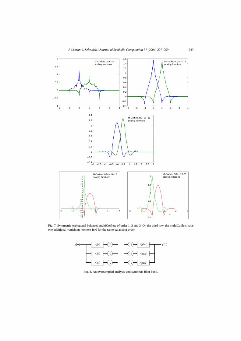
Using this approach, we have been able to construct all the minimal length ortho-normal multiCoiflets with compact support, symmetric scaling functions, symmet-ric/antisymmetric wavelets for order 1, 2 and 3 of balancing.Fig. 7 shows the smoothestscaling functions associated to multiCoiflets with these properties. More details are avail-able inLebrun(2000), Lebrun(2003) and alsoSelesnick(1999) where a family of cardinalmultiwavelets is constructed (these can be seen as generalized multiCoiflets with the centerof mass of the scaling functions not on the integer grid anymore).

7. Wavelet tight frames

This section describes a family of wavelet tight frames, or ‘overcomplete’ bases in-troduced inSelesnick(2000a) andSelesnick and Sendur(2000). With frames some fun-damental properties can be better realized than is possible with bases. For example, bet-ter time-frequency localization can be achieved. In addition, wavelet frames can be shift-invariant, while wavelet bases cannot be. In general, frames provide more degrees of free-dom to carry out design. Several applications have benefited from the use of frames, for ex-ample, denoising (Coifman and Donoho, 1995; Guo et al., 1995; Lang et al., 1995, 1996).

This section describes the design of frames that are analogous to theDaubechies(1992) orthonormal wavelets—that is, the design of minimal length filters with polynomialproperties, but now in the case of oversampled filter banks. The wavelets presented beloware much smoother than what can be achieved in the critically sampled case.

The nonlinear design equations that arise are then solved using Gröbner bases.As Grobner bases are used here, we are able to obtain zero wavelet moments forwavelets of minimal length, in contrast to earlier work on wavelet tight frames of thistype (Chui and He, 2000; Ron and Shen, 1997). Some later works (Chui et al., 2002;Daubechies et al., 2001) also describe other methods not based on Gröbner bases.

7.1. Preliminaries

The wavelet tight frames developed in this section are based on a single scaling functionφ(t) and two distinct waveletsψ1(t) andψ2(t). Following the multiresolution framework,φ, ψ1, ψ2 satisfy the dilation and wavelet equations

φ(t) = √2∑

n

h0(n)φ(2t − n)

ψi (t) =√

2∑

n

hi (n)φ(2t − n), i = 1,2.

Corresponding toφ, ψ1, ψ2, we have the scaling filterh0(n), the two wavelet filtersh1(n)andh2(n), and the oversampled filter bank illustrated inFig. 8.

Let φk(t) = φ(t − k) andψi, j ,k(t) = ψi (2 j t − k) for i = 1,2. Then{φk(t), ψi, j ,k(t) :j , k ∈ Z, j ≥ 0, i ∈ {0,1}} forms a tight frame forL2(R) if any square integrable signalf (t) can be expanded as

f (t) =∞∑

k=−∞c(k)φk(t)+

∞∑j=0

∞∑k=−∞

(d1( j , k)ψ1, j ,k(t)+ d2( j , k)ψ2, j ,k(t)) (32)


M-Coiflets O1+3–7scaling functions

M-Coiflets O2+ 7–11scaling functions

scaling functions M-Coiflets O3+15–19

–1

–0.5

0

0.5

1

1.5

2

–0.4

–0.2

0

0.2

0.4

0.6

0.8

1

1.2

1.4

1.6

–0.4

–0.2

0

0.2

0.4

0.6

0.8

1

1.2

1.4

–2 –1 0 1 2 3 4 –3 –2 –1 0 1 2 3 4

–1.5 –1 –0.5 –0 0.5 1 1.5 2 2.5 3–2

x

M-Coiflets O2++ 11–15scaling functions

–0.8–0.6–0.4–0.2

00.20.40.60.8

11.21.41.61.8

22.22.42.62.8

–2 –1 1 2 3 –2 –1 1 2 3x

M-Coiflets O3++ 19-23scaling functions

–0.5

0.5

1

1.5

2

Fig. 7. Symmetric orthogonal balanced multiCoiflets of order 1, 2 and 3. On the third row, the multiCoiflets haveone additional vanishing moment in 0 for the same balancing order.

y(n)x(n)↑ 2 ↑2

↑ 2 ↑2

↑ 2 ↑2

H0(z) H0(1/z)

H1(1/z)

H2(1/z)

H1(z)

H2(z)

Fig. 8. An oversampled analysis and synthesis filter bank.


where

c(k) =∫

f (t)φk(t) dt, di ( j , k) =∫

f (t)ψi, j ,k(t) dt, i = 1,2.

That is, a function can be expanded in a tight frame in a way that resembles an expansionin an orthonormal basis. Like orthonormal bases, tight frames have a Parseval’s relation:

‖ f ‖2 =∞∑

k=−∞|c(k)|2+

∞∑j=0

∞∑k=−∞

(|d1( j , k)|2+ |d2( j , k)|2).

By standard multirate identities, the PR conditions can be written as

H0(z)H0(z−1)+ H1(z)H1(z

−1)+ H2(z)H2(z−1) = 2 (33)

H0(−z)H0(z−1)+ H1(−z)H1(z

−1)+ H2(−z)H2(z−1) = 0. (34)

7.2. Zeros atω = 0, ω = πLet K0 denote the number of zerosH0(ejω) has atω = π . For i = 1,2, let Ki denote

the number of zerosHi (ejω) has atω = 0.

(z+ 1)K0 | H0(z), (z− 1)K1 | H1(z), (z− 1)K2 | H2(z). (35)

For orthonormal bases (ψ2(t) = 0), it is necessary thatK0 = K1, so no distinction needbe made betweenK0 andK1. However, for tight wavelet frames of the form (32), it is notnecessary thatK0 = K1 = K2. K0 denotes the degree of polynomials representable byshifts ofφ(t). K1 andK2 denote the number of zero moments of the wavelet filtersh1(n)andh2(n), providedK0 ≥ K1, andK0 ≥ K2.

The value ofK0 influences the degree of smoothness ofφ (and therefore ofψi ). On theother hand, the valuesK1 andK2 indicate what polynomials are annihilated (compressed)by the given signal expansion. In contrast to orthonormal wavelet bases, with a tight frameone has the possibility to control these parameters more freely. If it is desired for a givenclass of signals that the wavelets have two zero moments (for example), then the remainingdegrees of freedom can be used to achieve a higher degree of smoothness by makingK0greater thanK1 andK2.

7.3. Example

We seek to design FIR filtersh0,h1,h2 that generate tight frames of the form describedin (32). We seek the shortest filtershi having a prescribed number of zeros atz = −1 andz = 1 (specified by the valuesKi ) that satisfy the tight frame conditions (33) and (34). Inthe examples, we ask thatK1 = K2. If they are unequal, then one wavelet annihilates morepolynomials than the other, or one wavelet is doing ‘more work’ than the other.

Note that the conditions (33) and (34) are nonlinear equations in the filter coefficientshi (n). For the design problems considered below, these nonlinear design equations arehandled using Gröbner bases.

We ask thatK0 = 5, K1 = K2 = 2. It was found that the shortest filtersh0, h1,h2 satisfying (33) and (34) are of length 7, 7, and 5, respectively. By utilizing Gröbnerbasis methods it is possible to obtain exact expressions forhi (n). (Singular(Greuel et al.,2000) was used for the Gröbner basis calculations.) The original design equations have


φ

ψ1

ψ2

h0

h1

h2

–0.5

0

0.5

1

–0.5

–0.5

–1

0

0.5

1

–1

0

0.5

1

–0.5

0

0.5

1

–0.5

–0.5

–1

0

0.5

1

–1

0

0.5

1

0

0.5

1

1.5

0

0.5

1

1.5

0

0.5

1

1.5

0 1 2 3 4 5 6 0 1 2 3 4 5 6 0 0.2 0.4 0.6 0.8 1

0 1 2 3 4 5 6 0 1 2 3 4 5 6 0 0.2 0.4 0.6 0.8 1

0 1 2 3 4 5 6 0 1 2 3 4 5 6 0 0.2 0.4 0.6 0.8 1

|H0|

|H1|

|H2|

Fig. 9. The generators of a wavelet tight frame with parametersK0 = 5, K1 = K2 = 2.

only rational coefficients, and we were able to obtainexplicit expressions forhi (n) interms of radicals. The expressions obtained forhi (n) are too long to include here, but areavailable from I.S.

The filtersh0, h1, h2 were found by converting the nonlinear design equations into a drlGrobner basis, then converting that into a lex Gröbner basis, and factorizing that into twoGrobner bases. Then the ordering of the variables was changed, to obtain two lex Gröbnerbases which are more compact. However, if this ordering is used from the beginning, thenthe original lex Gröbner basis does not factor. All minimal-length pairs of scaling filterscan be found by solving these 2 Gröbner bases. The Gröbner bases indicate that there are32 solutions to the nonlinear design equations (16 solutions from each part).

As in the orthonormal case, there are multiple solutions to this problem. However,in contrast to the orthonormal case, (i) the distinct solutions do not all share the sameautocorrelation, and (ii) not all of the spectral factors of each autocorrelation are solutions.In this example, there are 4 distinct solutions, not counting their time-reversals (hi (−n))and negations (−hi (n)). One of those 4 solutions is shown inFig. 9. The other 3 solutionsare tabulated on the webpage of I.S.

8. Conclusion

In conclusion, for many of the design problems arising in the construction of specializedwavelets and filter banks, Gröbner bases are a natural tool. And although the highcomputational and memory cost of Gröbner bases limits their utility, we are able to obtainsolutions of practical interest, as illustrated in this paper. Indeed, we have introducedexamples of multiwavelet bases and wavelet frames that we could not have obtainedwithout them. As software for Gröbner bases, and the related theory, is advancing withtime, we expect Gröbner bases will be no less useful for future problems arising in thedesign of filters and transforms for signal processing.


Acknowledgements

J.L. warmly thanks Martin Vetterli for having made Gröbner Basesunavoidablefromthe start of his Ph.D. thesis. A big credit has to be given also to Jean-Charles Faugèreand Fabrice Rouillier for making their wonderful software available and a very specialthank you goes to Gil Strang and Thierry Blu for their useful remarks and fruitful help.This work was partly supported by the Swiss National Science Foundation under grant2100-043136.95/1. I.S. would like to thank Richard Baraniuk and Rob Nowak for bringingGrobner bases to his attention in 1995. He also gratefully acknowledges support by theNSF under CAREER grantCCR-987452.

Appendix A. Computation algebra digest

A.1. Introducing Grobner bases

In this paragraph, we will review the major ideas involved in the computation ofGrobner bases. We will not go much into the details, since many good books ranging fromintroductory (Froberg, 1997) to advanced level (Cox et al., 1992, 1998) have been writtenon this now popular subject. We will rather develop an intuitive understanding of what aGrobner basis is and describe some ways to compute them by using analogies to linearalgebra.We define a multivariate polynomialp to be a finite sum of terms

∑α cαxα, where a term

cαxα is the product of a coefficientcα and a monomialxα. One can draw an analogybetween solving linear systems that can be seen as the study of the associated vectorsubspace and solving a polynomial system that can be seen as the study of the associatedideal. Namely, a polynomial system of equations is defined by a list{p1, . . . , pN} ofmultivariate polynomials with rational coefficients (p1, . . . , pN ∈ Q[x1, . . . , xn]). Weassociate to this system the generated idealI = 〈p1, . . . , pN〉 i.e. the smallest idealcontaining p1, . . . , pN as well as

∑Nk=1 hk pk, for any h1, . . . ,hN ∈ Q[x1, . . . , xn].

Intuitively, the idea is that the polynomialsp1, . . . , pN have a common zero iff anypolynomial of the idealI vanishes also at that location. It is then equivalent to study asystem of polynomial equations or the ideal generated by the polynomials.For a set of linear equations, the Gauss elimination algorithm enables us to compute anequivalent triangular system by canceling the leading term of each equation. A similaralgorithm (called theBuchbergeralgorithm) can be developed for the case of multivariatepolynomials. An important aspect of the Gauss elimination algorithm is in the choice ofthe pivots that are used during the triangularization of the system. For the same reasons, thefirst thing we have to define is an ordering on the monomials (that needs to be compatiblewith polynomial multiplication). We introduce here two monomial orderings:

• Thelexicographicordering, abbreviatedlex. This is the ordering used in dictionaries.• Thedegree reverse lexicographicorder, abbreviateddrl. This is a modified reversed

lexicographic ordering taking first into account the total degree of the polynomials.

We then introduce the leading term lt(p,<) of a polynomialp as its term with thehighest order according to the ordering<, we also introduce the leading monomial


lm(p,<) as the leading term with a coefficient normalized to 1 and lc(p,<) as the leadingcoefficient. Notice that when no doubt remains, we will omit to mention the ordering. Ina very similar way to what is done in the Gauss elimination algorithm, we introduce theS-polynomialas a monomial combination of two polynomials so as to cancel their leadingterms.

Spol(p1, p2) := lcm(lt(p1), lt(p2))

lt(p1)p1− lcm(lt(p1), lt(p2))

lt(p2)p2 (36)

where lcm stands for theleast common multipleof a set of polynomials. For example,with the<lex ordering(x > y > z), p1 = 2x3y + · · · and p2 = x2y2 + · · ·, we getSpol(p1, p2) = yp1−2xp2. We have canceled the leading terms ofp1 andp2. Of particularinterest is when Spol(p1, p2) = p1−qp2 for some polynomialq (e.g.p1 = 3x3y+· · · andp2 = xy+ · · ·). In that case, we say thatp1 is reducibleby p2 and thatq is thereductionof p1 by p2. This reduction can easily be extended to the reduction of a polynomial by anordered list of polynomials,L = [q1, . . . ,qN ].

We shall emphasize the importance of the order in which the reductions are done: thesame set of polynomials reordered in a different list will usually give rise to a differentoutput of the reduction process. However, for any list of polynomials there exists anequivalent list such that the order has no influence anymore.

The famous Buchberger algorithm transforms by a progressive reduction process ageneral ordered list of polynomials generating the idealI into an equivalent one that makesit much easier to deal with the ideal generated. The list of polynomials obtained by theBuchberger algorithm is called a Gröbner basis. One of the major properties of Gröbnerbases is that it makes it algorithmically easy to verify if a given polynomial belongs or notto the ideal generated.

The major features of the Buchberger algorithm is that the list obtainedG := [g1, . . . ,gN ] still generatesI and satisfies the following Gröbner basis definition:Spol(gi , gj ) reduces to 0 moduloG, for everygi , gj ∈ G. It is easily seen that Gröbnerbases have the following equivalent characterizations:

• f ∈ I iff f reduces to 0 moduloG (Reduce( f,G) = 0).• The leading term of any element ofI is divisible by at least one leading term lt(gi )

of G.

For an idealI , let 〈LT(I )〉 denote the ideal of leading terms ofI , i.e. the ideal generatedby the set of leading terms LT(I ) := {cxα | ∃ f ∈ I , lt( f ) = cxα}. We then get thatG := [g1, . . . , gN ] is a Grobner basis ofI iff the ideal of leading terms ofI is generatedby the leading terms ofG i.e. 〈LT(I )〉 = 〈lt(g1), . . . , lt(gN)〉.

Usually, one can compute infinitely many Gröbner bases. However, among all these,one satisfies some nicer properties: every elementgi of the basisG has its leading termnormalized (coefficient equal to 1) and∀gi ∈ G, no term ofgi is divisible by a leadingmonomial lm(gj )( j �= i ). This particular basis is called thereducedGrobner basis: oneverifies that for a given monomial ordering monomial<, a non-empty polynomial idealalways has a unique reduced Gröbner basis. With the reduced Gröbner basis, we get thevery nice feature that the output of Reduce(p,G) does not depend anymore on the orderof the polynomials in the list: Reduce(·,G) becomes thecanonical reductionmoduloI .


In the case< is lexicographic, the reduced Gröbner basis has a very nice structure.Namely, the reduced Buchberger algorithm gives a union of triangular arrays ofpolynomials of the following form:

h(d+1)0 (x1, . . . , xd)

(x

kd+1d+1 +

h(d+1)1 (x1,...,xd )

h(d+1)0 (x1,...,xd )

xkd+1−1d+1 + h(d+1)

2 (x1,...,xd)

h(d+1)0 (x1,...,xd)

xkd+1−2d+1 + · · ·

)

h(d+2)0 (x1, . . . , xd+1)

(x

kd+2d+2 +

h(d+2)1 (x1,...,xd+1)

h(d+2)0 (x1,...,xd+1)

xkd+2−1d+2 + h(d+2)

2 (x1,...,xd+1)

h(d+2)0 (x1,...,xd+1)

xkd+2−2d+2 + · · ·

). . .

h(n)0 (x1, . . . , xn−1)

(xknn + h(n)1 (x1,...,xn−1)

h(n)0 (x1,...,xn−1)xkn−1n + h(n)2 (x1,...,xn−1)

h(n)0 (x1,...,xn−1)xkn−2n + · · ·

)(37)

whered gives the number of remaining degrees of freedom of the system when all of theequations are satisfied (x1, . . . , xd are now parameters).d is called the algebraic dimensionof the ideal: the solutions of a system of polynomial equations can be seen as a geometricvariety that can be classified by its algebraic dimension:d = 0: finite number of isolatedpoints,d = 1: curves,d = 2: surfaces and so on. In case the system has different kindsof solutions (e.g. isolated points and curves), the global dimension is just the maximumdimension of each component.

Whend = 0, i.e. when the system has a finite number of solutions, we get that the firstequation becomes a univariate polynomial equation and we can then rewrite the reducedGrobner basis as:

xk11 + g1(x1) degx1

(g1) < k1

xk22 + g2(x1, x2) degx2

(g2) < k2

· · · · · ·xkn

n + gn(x1, x2, . . . , xn) degxn(gn) < kn.

(38)

On such a system, it is now easy to carry out many operations like counting exactly allcomplex/real solutions including the multiplicity, isolating the real roots with the desiredprecision or approximating the complex roots (Gonzalez-Vega et al., 1999). For example,to numerically solve the system: first solve the univariate equationxk1

1 + g1(x1) = 0, thenrecursively substitute and solve the next equations. Moreover, in the case the variablex1is separating (intuitively two solutions cannot have the same first component; a rigorousdefinition is given in the next section), we get thatk2 = k3 = · · · = kn = 1. The system isthen of the form

g1(x1)

x2+ g2(x1)

· · · · · ·xn + gn(x1).

(39)

and all we have to do is to solveg1(x1) = 0 and substitute in the other equations. This iscalled theShape lemmacase (Rouillier, 1999).

A.2. Linear algebra methods

The necessary time to compute a reduced Gröbner basis by the Buchberger algorithmdepends strongly on the monomial ordering that is used. In general, computing a


reduced Gröbner basis for the lexicographic ordering is much more time and memoryconsuming than computing the corresponding drl Gröbner basis. However, this additionalcomputational cost may be worth it because, as seen before, the lexicographic orderingprovides a triangular like structure (similar to the one obtained by Gauss elimination) thatis really suitable for further processing. Fortunately, recent algorithms enable the efficientcomputation of lexicographic Gröbner bases by using an alternative approach:

• First, we compute a Gröbner basis for the drl ordering, using, for example, thestandard Buchberger algorithm (note that the algorithm can be highly improved byusing heuristics for the choice of the critical pairs and the reductors in the reducingprocess). An even better approach is to completely suppress the influence of thesechoices, by in factnot choosinganymore as introduced byFaugere (1999) in hisF4 algorithm: instead of choosing one critical pair, we take a subset of criticalpairs and reduce this set. By using a linear algebra approach to deal with the pairs,the algorithm can be made extremely efficient for the computation of drl Gröbnerbases. An implementation named FGb of this algorithm can be tested on the web athttps://www-calfor.lip6.fr• Finally, we compute the lexicographic Gröbner basis from the drl one by a change of

ordering. For the case when the ideal is zero-dimensional, a very efficient algorithmcalled FGLM (Faugere et al., 1994) has been developed using again a linear algebraapproach. Implementations of this algorithm are now available in most of thecomputer algebra programs.

We will now give some details on how the linear algebra approach works. Again, formore details, the reader can read the survey on the subject byMourrain (1999). Startingfrom a list P of polynomials such that the generated idealI = 〈P〉 is zero-dimensional,we show that the quotient spaceA := Q[x1, . . . , xn]/I inherits a structure of finite-dimensional algebra. Namely, assuming a reduced Gröbner basisG := [g1, . . . , gN ] forsome ordering< (typically drl), any element ofA has the formp = Reduce(p,G) forsome p ∈ Q[x1, . . . , xn]. Since〈LT(I )〉 = 〈lt(g1), . . . , lt(gN)〉, we easily construct alinear basis ofA from the set of monomials{xα | xα /∈ 〈LT(I )〉}, by taking in increasingorder the monomials under the staircase, i.e. thexα that are not a multiple of lt(gi ) (sincethis implies thatxα = Reduce(xα,G) = xα). The linear basisB := {ω1, . . . , ωd} obtainedthis way is called themonomial basisof A. Finally, constructing the multiplication table[ωiω j ]i, j of A, we get a full description of the linear algebraic framework in which wewill deal with the polynomials.

Now, any elementp ∈ A can be expressed as a vector[p] since p = ∑dk=1[p]iωi .

The FGLM algorithm can then be described using linear algebra inA. The lexicographicGrobner basis is obtained by detecting linear combinations of monomials inA. The ideais to construct in parallel the lex Gröbner basisG<lex and a full rankd × d matrix G,by scanning the monomialsxα in increasing lex ordering (starting from 1). There are twopossibilities:

1. [xα] is linearly dependent of the previous vectors put inG (i.e. we can write[xα] = ∑

k ck[xβk]), then we addgα := xα −∑k ckxβk to G<lex (namely,gα ∈ Iand lt(gα) = xα).

2. [xα] is linearly independent of the previous vectors put inG, then add[xα] to G.

https://www-calfor.lip6.fr


Repeat the scan until rank(G) = d; G<lex is then a lex Gröbner basis ofI .

A.3. The rational univariate representation

In many situations, the computation of a lex Gröbner basis of the idealI is a bit ofan overkill in the sense that in fact, all we are really interested in, is a good descriptionof the set of solutions of the system,ZC(I ) := {α ∈ Cn | ∀p ∈ P, p(α) = 0}(we will denote byµ(α) the multiplicity of a solutionα). In the approach, alternativeto FGLM, developed byRouillier (1999) andGonzalez-Vega et al.(1999), one constructsa list {χu(t), gu(1, t), gu(x1, t), . . . , gu(x1, t)} of polynomials ofQ[x1, . . . , xn] such that:if α is a solution of the system, thenu(α) is a root ofχu(t) with the same multiplicity andconversely, ifζ is a root ofχu(t), then[

gu(x1, ζ )

gu(1, ζ ),

gu(x2, ζ )

gu(1, ζ ), . . . ,

gu(xn, ζ )

gu(1, ζ )

](40)

is a solution of the system with the same multiplicity. Hence,ZC(I ) is fully characterized.The basic tool of this method is the computation of linear operatorMu onA associated topolynomialsu,

Mu : A→ Af &→Mu f := u f . (41)

We identify Mu with its Cd×d matrix representation in the monomial basis of A. Thismatrix is easily computed by expressinguωi in the monomial basis, which gives the ithcolumn ofMu.The computations ofMu give much important information onZC(I ) and the system ingeneral. From these matrices, we can construct a bijection betweenZC(P), the set ofsolutions of the system, and the roots of the univariate polynomialχu(t). All we have todo now to getZC(P) is to isolate the roots ofχu(t). We then derive the solutions of thesystem using the RUR. The isolation of roots is usually a difficult problem. However, inthe case we are only interested in the real solutions of the system, we can locate them veryefficiently by computing the signature of trace matrices (Pedersen et al., 1993).Alternatively, we can also factorizeχu(t). We construct this way local algebras that enableus to simplify the problem of isolating the roots by lowering the degrees of characteristicpolynomials in the RURs.In short, the RUR approach appears to be a very efficient alternative to the computation ofa lexicographic Gröbner basis: as detailed inRouillier (1999), it is computationally easierto compute a RUR than to apply the FGLM algorithm and the characteristic polynomialχu(t) is usually easier to deal with thang1(x1), the leading polynomial of the lexicographicGrobner basis. Besides, when the polynomial system is overdetermined, similar linearalgebra methods (Giusti and Schost, 1999) have been developed to completely avoid thecomputation of Gröbner bases.

References

Abdelnour, A.F., Selesnick, I.W., 2001. Nearly symmetric orthogonal wavelet bases. In: ICASSP,Proc. IEEE Int. Conf. Acoust., Speech, Signal Processing, May, 2001.


Alpert, B., 1993. A class of bases in2 for the sparse representation of integral operators. SIAM J.Math. Anal. 24 (1), 246–262.

Burrus, C.S., Gopinath, R.A., Guo, H., 1998. Introduction to Wavelets and Wavelets Transforms—A Primer. Prentice-Hall.

Chui, C.K., He, W., 2000. Compactly supported tight frames associated with refinable functions.Appl. Comput. Harmon. Anal. 8 (3), 293–319.

Chui, C.K., He, W., Stöckler, J., 2002. Compactly supported tight and sibling frames with maximumvanishing moments. Appl. Comp. Harmonic Anal. 13, 224–262.

Chui, C.K., Lian, J.-A., 1996. A study of orthonormal multi-wavelets. Appl. Numer. Math. 20 (3),273–298.

Cohen, A., 1992. Biorthogonal wavelets. In: Chui, C.K. (Ed.), Wavelets: A Tutorial in Theory andApplications. Academic Press, New York.

Cohen, A., Daubechies, I., Plonka, G., 1997. Regularity of refinable function vectors. J. FourierAnal. Appl. 3, 295–324.

Coifman, R.R., Donoho, D.L., 1995. Translation-invariant de-noising. In: Antoniadis, A. (Ed.),Wavelets and Statistics. Springer-Verlag Lecture Notes.

Cox, D., Little, J., O’Shea, D., 1992. Ideals, Varieties and Algorithms. Springer-Verlag.Cox, D., Little, J., O’Shea, D., 1998. Using Algebraic Geometry. Springer-Verlag.Crochiere, R.E., Webber, S.A., Flanagan, J.L., 1976. Digital coding of speech in sub-bands. Bell

Syst. Tech. J. 55 (8), 1069–1085.Croisier, A., Esteban, D., Galand, C., 1976. Perfect channel splitting by use of interpola-

tion/decimation/tree decomposition techniques. In: Int. Conf. on Inform. Sciences and Systems,Patras, Greece, 1976, pp. 443–446.

Daubechies, I., 1988. Orthonormal bases of compactly supported wavelets. Commun. Pure Appl.Math. 41, 909–996.

Daubechies, I., 1992. Ten Lectures on Wavelets. SIAM.Daubechies, I., Han, B., Ron, A., Shen, Z., 2001. Framelets: MRA-based constructions of wavelet

frames (preprint).Donovan, G.C., Geronimo, J.S., Hardin, D.P., Massopust, P.R., 1996. Construction of orthogonal

wavelets using fractal interpolation functions. SIAM J. Math. Anal. 27 (4), 1158–1192.Faugere, J.-C., 1999. A new efficient algorithm for computing Gröbner bases (F4). J. Pure Appl.

Algebra 139, 61–88. Available fromhttps://www-calfor.lip6.fr.Faugere, J.-C., de Saint-Martin, F.M., Rouillier, F., 1998. Design of regular nonseparable bidi-

mensional wavelets using Gröbner basis techniques. IEEE Trans. Signal Proc. 46 (4), 845–857.Faugere, J.-C., Gianni, P., Lazard, D., Mora, T., 1994. Efficient computation of zero-dimensional

Grobner bases by change of ordering. J. Symbolic Comput. 16 (4), 329–344.Froberg, R., 1997. An Introduction to Gröbner Bases. John Wiley & Sons.Geronimo, J.S., Hardin, D.P., Massopust, P.R., 1994. Fractal functions and wavelet expansions

based on several scaling functions. J. Approx. Theory 78.Gonzalez-Vega, L., Rouillier, F., Roy, M.-F., 1999. Symbolic recipes for polynomial system

solving. In: Some Tapas of Computer Algebra. Springer-Verlag.Greuel, G.-M., Pfister, G., Schönemann, H., 2000. Singular reference manual. University of

Kaiserslautern. Available fromhttp://www.singular.uni-kl.de.Giusti, M., Schost, E., 1999. Solving some overdetermined polynomial systems. In: ISSAC, Proc.

Int. Symp. on Symbolic and Algebraic Computation, July 1999.Guo, H., Lang, M., Odegard, J.E., Burrus, C.S., 1995. Nonlinear shrinkage of undecimated

DWT for noise reduction and data compression. In: Proc. Int. Conf. on Digital Signal Processing,Limassol, June 1995.

Heil, C., Strang, G., Strela, V., 1996. Approximations by translates of refinable functions. Numer.Math. 73, 75–94.

https://www-calfor.lip6.fr

http://www.singular.uni-kl.de


Jia, R.Q., Lei, J.J., 1993. Approximation by multi-integer translates of functions having globalsupport. J. Approx. Theory 72, 2–23.

Lang, M., Guo, H., Odegard, J.E., Burrus, C.S., Wells Jr., R.O., 1995. Nonlinear processing ofa shift-invariant DWT for noise reduction. SPIE Conference on Wavelet Applications, Orlando,FL, April, 1995, vol. 2491.

Lang, M., Guo, H., Odegard, J.E., Burrus, C.S., Wells Jr., R.O., 1996. Noise reduction using anundecimated discrete wavelet transform. IEEE Signal Process. Lett. 3 (1), 10–12.

Lawton, W., Lee, S.L., Shen, Z., 1996. An algorithm for matrix extension and wavelet construction.Math. Comp. 65, 723–737.

Lebrun, J., 2000. Balancing MultiWavelets. Ph.D. Thesis, Swiss Federal Institute of Technology(EPFL), Lausanne.

Lebrun, J., Vetterli, M., 1998. Balanced multiwavelets—Theory and design. IEEE Trans. SignalProc. 46 (4), 119–125.

Lebrun, J., 2003. Theory and design of multiCoiflets, submitted.Lebrun, J., Vetterli, M., 2001. High order balanced multiwavelets: theory, factorization and design.

IEEE Trans. Signal Proc. 49 (9), 1918–1930.Mallat, S., 1989. A theory for multiresolution signal decomposition: the wavelet representation.

IEEE Trans. Pattern Anal. Mach. Int. 11 (7), 674–693.Mallat, S., 1998. A Wavelet Tour of Signal Processing. Academic Press.Massopust, P.R., Ruch, D.K., Van Fleet, P., 1996. On the support properties of scaling vectors.

Appl. Comput. Harmon. Anal. 3, 229–238.Mintzer, F., 1985. Filters for distortion-free two-band multirate filter banks. IEEE Trans. Acoust.

Speech Signal Proc. 33 (3), 626–630.Mourrain, B., 1999. An introduction to linear algebra methods for solving polynomial equations.

In: Lipitakis, E.A. (Ed.), Proc. HERCMA’ 9, pp. 179–200.Park, H., Kalker, T., Vetterli, M., 1997. Groebner bases and multidimensional FIR multirate

systems. J. Multidim. Syst. Signal Proc. 8, 11–30.Pedersen, P., Roy, M.-F., Szpirglas, A., 1993. Computational Algebraic Geometry. Birkhauser,

pp. 203–223.Plonka, G., 1997. Approximation order provided by refinable function vectors. Const. Approx. 13,

221–244.Plonka, G., Strela, V., 1998. Construction of multi-scaling functions with approximation and

symmetry. SIAM J. Math. Anal. 29, 481–510.Rioul, O., 1993. A discrete-time multiresolution theory. IEEE Trans. Signal Proc. 41 (8), 2591–2606.Ron, A., Shen, Z., 1997. Affine systems inL2(R

d): the analysis of the analysis operator. J. Funct.Anal. 148, 408–447.

Rouillier, F., 1999. Solving zero-dimensional systems through the rational univariate representation.J. Appl. Alg. Eng., Comm. Comp. 9, 433–461.

Selesnick, I.W., 1998. Multiwavelet bases with extra approximation properties. IEEE Trans. SignalProc. 46, 2898–2908.

Selesnick, I.W., 1999. Interpolating multiwavelet bases and the sampling theorem. IEEE Trans.Signal Proc. 47 (6), 1615–1621.

Selesnick, I.W., 2000a. Smooth wavelet tight frames with zero moments: design and properties.In: Proc. of the Ninth IEEE DSP Workshop.

Selesnick, I.W., 2000b. Balanced multiwavelet bases based on symmetric FIR filters. IEEE Trans.Signal Proc. 48 (1), 184–191.

Selesnick, I.W., Burrus, C.S., 1998. Maximally flat low-pass FIR filters with reduced delay. IEEETrans. Circuits Syst. II 45 (1), 53–68.

Selesnick, I.W., Sendur, L., 2000. Iterated oversampled filter banks and wavelet frames. In: SPIEConference on Wavelet Applications, San Diego, August, 2000.


Smith, M.J.T., Barnwell, T.P., 1984. A procedure for designing exact reconstruction filter banks fortree structured sub-band coders. In: Proc. IEEE Int. Conf. Acoust., Speech, and Signal Proc., SanDiego, CA, March, 1984.

Strang, G., Nguyen, T., 1996. Wavelets and Filter Banks, Wellesley Cambridge Press, Boston.Strang, G., Strela, V., 1995. Short wavelets and matrix dilation equations. IEEE Trans. Signal Proc.

43, 108–115.Tian, J., Wells Jr., R.O., Odegard, J.E., Burrus, C.S., 1997. Coifman wavelet systems:

approximation, smoothness, and computational algorithms. In: Bristeau, M-O. et al. (Eds.),Computational Science for the 21st Century. John Wiley & Sons.

Vaidyanathan, P.P., 1993. Multirate Systems and Filter Banks. Prentice-Hall, Englewood Cliffs, NJ.Vetterli, M., Herley, C., 1992. Wavelets and filter banks: theory and design. IEEE Trans. Signal

Proc. 40 (9), 2207–2232.Vetterli, M., Kovacevic, J., 1995. Wavelets and Subband Coding. Prentice-Hall, Englewood Cliffs,

NJ.Vetterli, M., Strang, G., 1994. Time-varying filter banks and multiwavelets. In: Proc. of the Sixth

IEEE DSP Workshop, Yosemite.Wei, D., Bovik, A.C., 1998. Generalized coiflets with nonzero-centered vanishing moments. IEEE

Trans. Circuits Syst. II 45 (8), 988–1001.

Documents

Grobner bases and wavelet design¨ - New York University