Embed Size (px)
DESCRIPTION
A TOOLBOX USING MATLAB TO CONTROL OPENDSS. This is the last version from ERPE concerning distributed generators and pvs
Citation preview
SANDIA REPORT SAND2014-20141 Unlimited Release Printed November 2014
Grid Integrated Distributed PV (GridPV) Version 2
Matthew J. Reno, Kyle Coogan
Prepared by Sandia National Laboratories Albuquerque, New Mexico 87185 and Livermore, California 94550
Sandia National Laboratories is a multi-program laboratory managed and operated by Sandia Corporation, a wholly owned subsidiary of Lockheed Martin Corporation, for the U.S. Department of Energy's National Nuclear Security Administration under contract DE-AC04-94AL85000. Approved for public release; further dissemination unlimited.

2
Issued by Sandia National Laboratories, operated for the United States Department of Energy
by Sandia Corporation.
NOTICE: This report was prepared as an account of work sponsored by an agency of the
United States Government. Neither the United States Government, nor any agency thereof,
nor any of their employees, nor any of their contractors, subcontractors, or their employees,
make any warranty, express or implied, or assume any legal liability or responsibility for the
accuracy, completeness, or usefulness of any information, apparatus, product, or process
disclosed, or represent that its use would not infringe privately owned rights. Reference herein
to any specific commercial product, process, or service by trade name, trademark,
manufacturer, or otherwise, does not necessarily constitute or imply its endorsement,
recommendation, or favoring by the United States Government, any agency thereof, or any of
their contractors or subcontractors. The views and opinions expressed herein do not
necessarily state or reflect those of the United States Government, any agency thereof, or any
of their contractors.
Printed in the United States of America. This report has been reproduced directly from the best
available copy.
Available to DOE and DOE contractors from
U.S. Department of Energy
Office of Scientific and Technical Information
P.O. Box 62
Oak Ridge, TN 37831
Telephone: (865) 576-8401
Facsimile: (865) 576-5728
E-Mail: [email protected]
Online ordering: http://www.osti.gov/bridge
Available to the public from
U.S. Department of Commerce
National Technical Information Service
5285 Port Royal Rd.
Springfield, VA 22161
Telephone: (800) 553-6847
Facsimile: (703) 605-6900
E-Mail: [email protected]
Online order: http://www.ntis.gov/help/ordermethods.asp?loc=7-4-0#online

3
SAND2014-20141
Unlimited Release
Printed November 2014
Grid Integrated Distributed PV (GridPV) Version 2
Matthew J. Reno
Photovoltaics and Distributed Systems Integration
Sandia National Laboratories
P.O. Box 5800
Albuquerque, New Mexico 87185-1033
Kyle Coogan
School of Electrical and Computer Engineering
Georgia Institute of Technology
777 Atlantic Drive NW
Atlanta, GA 30332-0250
Abstract
This manual provides the documentation of the MATLAB toolbox of functions for
using OpenDSS to simulate the impact of solar energy on the distribution system. The
majority of the functions are useful for interfacing OpenDSS and MATLAB, and they
are of generic use for commanding OpenDSS from MATLAB and retrieving
information from simulations. A set of functions is also included for modeling PV
plant output and setting up the PV plant in the OpenDSS simulation. The toolbox
contains functions for modeling the OpenDSS distribution feeder on satellite images
with GPS coordinates. Finally, example simulations functions are included to show
potential uses of the toolbox functions. Each function in the toolbox is documented
with the function use syntax, full description, function input list, function output list,
example use, and example output.

4
5
CONTENTS
1. Introduction ................................................................................................................................. 9 1.1. Objectives .......................................................................................................................... 9 1.2. Overview of GridPV Features ......................................................................................... 10
2. Download and Installation ........................................................................................................ 11
2.1. OpenDSS Installation....................................................................................................... 11 2.2. GridPV Installation Instructions ...................................................................................... 11 2.3. License Agreement .......................................................................................................... 11
2.4. GridPV Uninstall Instructions.......................................................................................... 13
3. OpenDSS................................................................................................................................... 15 3.1. OpenDSS Resources ........................................................................................................ 15
3.1.1. Websites ............................................................................................................. 15
3.1.2. Documents .......................................................................................................... 16
4. Getting Started with the Toolbox .............................................................................................. 17
4.1. OpenDSS COM Object Interface..................................................................................... 18 4.1.1. Initiating the COM Interface .............................................................................. 18
4.1.2. Compiling the Circuit ......................................................................................... 18 4.1.3. Getting Data into MATLAB from OpenDSS ..................................................... 19
4.1.4. Active Elements ................................................................................................. 21 4.1.5. Running Commands ........................................................................................... 21
4.1.6. Adding/Editing Elements ................................................................................... 22 4.2. Circuit Information Retrieval Using GridPV ................................................................... 22
4.2.1. Using the GridPV Get Functions ........................................................................ 23
4.2.2. Working with Structures from the Toolbox ....................................................... 23 4.3. Circuit Check Function .................................................................................................... 24
4.3.1. Running Circuit Check Function ........................................................................ 25 4.3.2. Interpreting Circuit Check Output ...................................................................... 25
4.4. Plotting Tutorial ............................................................................................................... 31
4.4.1. Plotting Circuits .................................................................................................. 31 4.4.2. User Interaction with Plots ................................................................................. 32 4.4.3. Plot Editing ......................................................................................................... 34
4.4.4. Plot Handles ....................................................................................................... 35 4.5. Coordinate Conversion Tutorial ...................................................................................... 37
4.5.1. Manual Conversion ............................................................................................ 38 4.5.2. UTM Conversion ................................................................................................ 40
4.6. Solar Tutorial ................................................................................................................... 41
4.6.1. Placing PV on the Circuit ................................................................................... 41 4.6.2. Adding Central PV ............................................................................................. 42 4.6.3. Adding Distributed PV ....................................................................................... 43
4.6.4. Editing Plant Info ............................................................................................... 43 4.6.5. Editing Power Factor .......................................................................................... 43 4.6.6. Creating the PV DSS Files ................................................................................. 46
4.7. Example Analyses ............................................................................................................ 47
4.7.1. Static Analysis .................................................................................................... 47
6
4.7.2. Time-Series Analysis in OpenDSS .................................................................... 48 4.7.3. Time-Series Analysis in MATLAB ................................................................... 49
5. Distribution System Models ..................................................................................................... 51 5.1. Example Circuit ............................................................................................................... 51
5.2. Links to Other Circuits ..................................................................................................... 52
6. Function Help Files ................................................................................................................... 53 6.1. OpenDSS Functions ......................................................................................................... 55
6.1.1. DSSStartup ......................................................................................................... 56 6.1.2. getBusCoordinatesArray .................................................................................... 57
6.1.3. getBusInfo .......................................................................................................... 58 6.1.4. getCapacitorInfo ................................................................................................. 60
6.1.5. getCoordinates .................................................................................................... 63 6.1.6. getGeneratorInfo ................................................................................................ 64 6.1.7. getLineInfo ......................................................................................................... 67 6.1.8. getLoadInfo ........................................................................................................ 71
6.1.9. getPVInfo ........................................................................................................... 75 6.1.10. getTransformerInfo .......................................................................................... 78
6.1.11. isinterfaceOpenDSS ......................................................................................... 83 6.2. Circuit Analysis Functions ............................................................................................... 84
6.2.1. circuitCheck ........................................................................................................ 85
6.2.2. findDownstreamBuses ........................................................................................ 86
6.2.3. findHighestImpedanceBus ................................................................................. 87 6.2.4. findLongestDistanceBus .................................................................................... 88 6.2.5. findSubstationLocation ...................................................................................... 89
6.2.6. findUpstreamBuses ............................................................................................ 90 6.3. Plotting Functions ............................................................................................................ 91
6.3.1. plotAmpProfile ................................................................................................... 92 6.3.2. plotCircuitLines .................................................................................................. 94 6.3.3. plotCircuitLinesOptions ................................................................................... 101
6.3.4. plotKVARProfile .............................................................................................. 103
6.3.5. plotKWProfile .................................................................................................. 106
6.3.6. plotMonitor ....................................................................................................... 109 6.3.7. plotVoltageProfile ............................................................................................ 111
6.4. Geographic Mapping Functions ..................................................................................... 116 6.4.1. initCoordConversion ........................................................................................ 117
6.4.2. createCircuitCoordConversion ......................................................................... 118 6.4.3. createCircuitCoordConversionUTM ................................................................ 119 6.4.4. plotGoogleMap ................................................................................................. 120
6.5. Solar Modeling Functions .............................................................................................. 123 6.5.1. placePVplant .................................................................................................... 124
6.5.2. createPVscenarioFiles ...................................................................................... 126
6.5.3. distributePV ...................................................................................................... 127
6.5.4. findMaxPenetrationTime .................................................................................. 128 6.5.5. IneichenClearSkyModel ................................................................................... 129 6.5.6. makePFoutputFunction .................................................................................... 130 6.5.7. makePFprofile .................................................................................................. 131
7
6.5.8. makePFschedule ............................................................................................... 133 6.5.9. makeVVCcurve ................................................................................................ 134 6.5.10. pvl_WVM ....................................................................................................... 135
6.6. Example Simulations ..................................................................................................... 139
6.6.1. examplePeakTimeAnalysis .............................................................................. 140 6.6.2. exampleTimeseriesAnalyses ............................................................................ 143 6.6.3. exampleVoltageAnalysis .................................................................................. 150
7. References ............................................................................................................................... 153
8. Distribution ............................................................................................................................. 155
FIGURES
Figure 1. Selecting an Element with Left Click. ........................................................................... 32 Figure 2. Selecting an Element with Left Click with Node View turned on. ............................... 32
Figure 3. Selecting an Element with Right Click. ........................................................................ 33 Figure 4. Using the toggle button to turn the secondary systems on/off. ..................................... 34
Figure 5. Avoid Using Plot Tools. ................................................................................................ 34 Figure 6. Use Property Editor to Modify. ..................................................................................... 35 Figure 7. Returning to the Default View. ..................................................................................... 35
Figure 8. Default plot and after using the handles structure to modify the capacitor markers. .... 36
Figure 9. Plotting your own buses. ............................................................................................... 37 Figure 10. Coordinate Conversion Initializer. .............................................................................. 37 Figure 11. Manual Coordinate Conversion GUI........................................................................... 38
Figure 12. Satellite Image Map Tools........................................................................................... 38 Figure 13. Feeder Map Tools. ....................................................................................................... 39
Figure 14. Coordinate File Backup Warning. ............................................................................... 39 Figure 15. Coordinate Conversion Successful. ............................................................................. 40 Figure 16. UTM Coordinate Conversion GUI. ............................................................................. 40
Figure 17. GUI of placePVPlant. .................................................................................................. 42
Figure 18. Central PV Location Prompt. ...................................................................................... 42 Figure 19. Distributed PV Location Prompt. ................................................................................ 43
Figure 20. Create Schedule GUI. .................................................................................................. 44 Figure 21. Create Function GUI. .................................................................................................. 45 Figure 22. Create VV Control GUI............................................................................................... 45 Figure 23. Circuit diagram for GridPV example circuit (EPRI Test Ckt24). ............................... 51 Figure 24. MATLAB Help Browser. ............................................................................................ 53
Figure 25. MATLAB GridPV Help Browser. .............................................................................. 53
TABLES
Table 1. Summary of EPRI Test Ckt24. ....................................................................................... 51
8
NOMENCLATURE
COM Component Object Model
DG Distributed Generation
DOE Department of Energy
EPRI Electric Power Research Institute
GUI Graphical user interface
IEEE Institute of Electrical and Electronics Engineers
LDC Line Drop Compensation
LTC Load Tap Changer
MW Megawatts (AC)
OpenDSS Open Distribution System Simulator™
PCC Point of Common Coupling
pu per unit
PV Photovoltaic
UTM Universal Transverse Mercator
VBA Visual Basic for Applications
WVM Wavelet Variability Model
9
1. INTRODUCTION
The power industry is seeing large amounts of distributed generation being added onto the
electric power distribution system. This presents a new set of issues, especially for renewable
generation with variable intermittent power output. It is important to precisely model the impact
of solar energy on the grid and to help distribution planners perform the necessary
interconnection impact studies. The variability in the load, throughout the day and year, and the
variability of solar, throughout the year and because of clouds, makes the analysis increasingly
complex. Both accurate data and timeseries simulations are required to fully understand the
impact of variability on distribution system operations and reliability.
This manual describes the functionality and use of a MATLAB toolbox for using OpenDSS to
model the variable nature of the distribution system load and solar energy. OpenDSS is an
electric power distribution system simulator that is open source software from the Electric Power
Research Institute (EPRI) [1]. OpenDSS is used to model the distribution system with
MATLAB providing the frontend user interface through a COM interface. OpenDSS is designed
for distribution system analysis and is very good at timeseries analysis with changing variables
and dynamic control. OpenDSS is command based and has limited visualization capabilities.
By bringing control of OpenDSS to MATLAB, the functionality of OpenDSS is utilized while
adding the looping, advanced analysis, and visualization abilities of MATLAB.
GridPV Toolbox is a well-documented tool for Matlab that can be used to build distribution grid
performance models using OpenDSS. Simulations with this tool can be used to evaluate the
impact of solar energy on the distribution system [2, 3]. The majority of the functions are useful
for interfacing OpenDSS and Matlab, and they are of generic use for commanding OpenDSS
from Matlab and retrieving information from simulations. A set of functions is also included for
modeling PV plant output and setting up the PV plant in the OpenDSS simulation. The toolbox
contains functions for modeling the OpenDSS distribution feeder on satellite images with GPS
coordinates.
The functions in the toolbox are categorized into five main sections in the manual: OpenDSS
functions, Solar Modeling functions, Plotting functions, Geographic Mapping functions, and
Example Simulations. Each function is documented with the function use syntax, full
description, function input list, function output list, and an example use. The function example
also includes an example output of the function.
1.1. Objectives
The GridPV Toolbox for MATLAB provides a set of well-documented functions for simulating
the performance of photovoltaic energy systems. Version 2 contains functions, example scripts,
and sample data files.
The toolbox was developed at Georgia Institute of Technology and Sandia National
Laboratories. It implements many of the models and methods developed at the Labs. Future
versions are planned that will add more functions and capability.
10
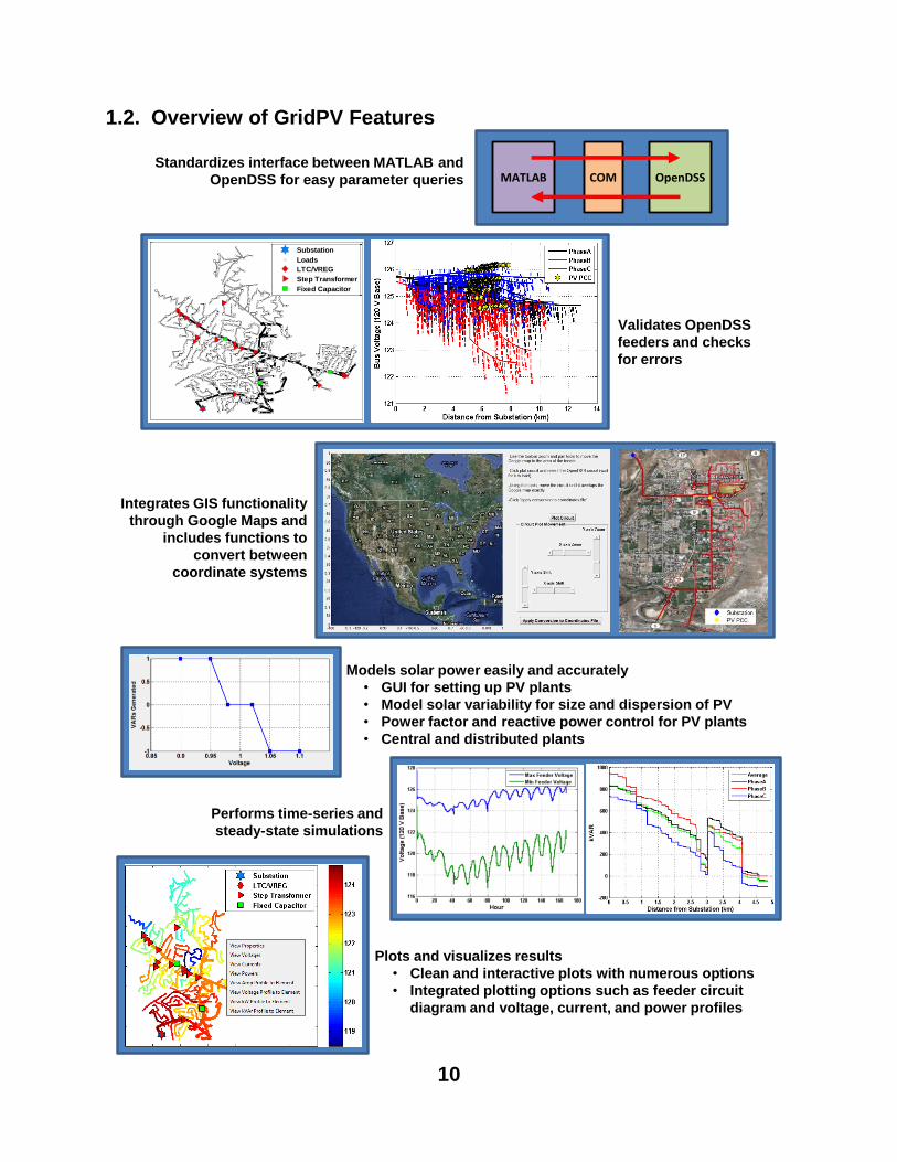
1.2. Overview of GridPV Features
Integrates GIS functionality
through Google Maps and
includes functions to
convert between
coordinate systems
Standardizes interface between MATLAB and
OpenDSS for easy parameter queries
Validates OpenDSS
feeders and checks
for errors
Performs time-series and
steady-state simulations
Models solar power easily and accurately
• GUI for setting up PV plants
• Model solar variability for size and dispersion of PV
• Power factor and reactive power control for PV plants
• Central and distributed plants
Plots and visualizes results
• Clean and interactive plots with numerous options
• Integrated plotting options such as feeder circuit
diagram and voltage, current, and power profiles
Substation
Loads
LTC/VREG
Step Transformer
Fixed Capacitor
Substation
Loads
LTC/VREG
Step Transformer
Fixed Capacitor
MATLAB COM OpenDSS
11
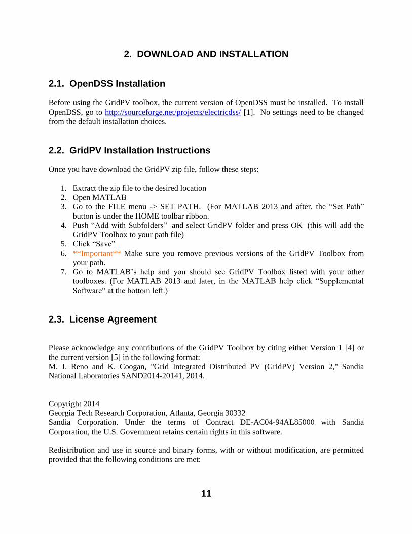
2. DOWNLOAD AND INSTALLATION
2.1. OpenDSS Installation
Before using the GridPV toolbox, the current version of OpenDSS must be installed. To install
OpenDSS, go to http://sourceforge.net/projects/electricdss/ [1]. No settings need to be changed
from the default installation choices.
2.2. GridPV Installation Instructions
Once you have download the GridPV zip file, follow these steps:
1. Extract the zip file to the desired location
2. Open MATLAB
3. Go to the FILE menu -> SET PATH. (For MATLAB 2013 and after, the “Set Path”
button is under the HOME toolbar ribbon.
4. Push “Add with Subfolders” and select GridPV folder and press OK (this will add the
GridPV Toolbox to your path file)
5. Click “Save”
6. **Important** Make sure you remove previous versions of the GridPV Toolbox from
your path.
7. Go to MATLAB’s help and you should see GridPV Toolbox listed with your other
toolboxes. (For MATLAB 2013 and later, in the MATLAB help click “Supplemental
Software” at the bottom left.)
2.3. License Agreement
Please acknowledge any contributions of the GridPV Toolbox by citing either Version 1 [4] or
the current version [5] in the following format:
M. J. Reno and K. Coogan, "Grid Integrated Distributed PV (GridPV) Version 2," Sandia
National Laboratories SAND2014-20141, 2014.
Copyright 2014
Georgia Tech Research Corporation, Atlanta, Georgia 30332
Sandia Corporation. Under the terms of Contract DE-AC04-94AL85000 with Sandia
Corporation, the U.S. Government retains certain rights in this software.
Redistribution and use in source and binary forms, with or without modification, are permitted
provided that the following conditions are met:
12
1. Redistributions of source code must retain the above copyright notice, this list of conditions
and the following disclaimer.
2. Redistributions in binary form must reproduce the above copyright notice, this list of
conditions and the following disclaimer in the documentation and/or other materials provided
with the distribution.
3. Neither the name of the Sandia National Laboratories nor the names of its contributors may be
used to endorse or promote products derived from this software without specific prior written
permission.
THIS SOFTWARE IS PROVIDED BY THE COPYRIGHT HOLDERS AND
CONTRIBUTORS "AS IS" AND ANY EXPRESS OR IMPLIED WARRANTIES,
INCLUDING, BUT NOT LIMITED TO, THE IMPLIED WARRANTIES OF
MERCHANTABILITY AND FITNESS FOR A PARTICULAR PURPOSE ARE
DISCLAIMED. IN NO EVENT SHALL THE COPYRIGHT HOLDER OR CONTRIBUTORS
BE LIABLE FOR ANY DIRECT, INDIRECT, INCIDENTAL, SPECIAL, EXEMPLARY, OR
CONSEQUENTIAL DAMAGES (INCLUDING, BUT NOT LIMITED TO, PROCUREMENT
OF SUBSTITUTE GOODS OR SERVICES; LOSS OF USE, DATA, OR PROFITS; OR
BUSINESS INTERRUPTION) HOWEVER CAUSED AND ON ANY THEORY OF
LIABILITY, WHETHER IN CONTRACT, STRICT LIABILITY, OR TORT (INCLUDING
NEGLIGENCE OR OTHERWISE) ARISING IN ANY WAY OUT OF THE USE OF THIS
SOFTWARE, EVEN IF ADVISED OF THE POSSIBILITY OF SUCH DAMAGE.
NOTICE:
For five (5) years from 07/15/2014, the United States Government is granted for itself and others
acting on its behalf a paid-up, nonexclusive, irrevocable worldwide license in this data to
reproduce, prepare derivative works, and perform publicly and display publicly, by or on behalf
of the Government. There is provision for the possible extension of the term of this license.
Subsequent to that period or any extension granted, the United States Government is granted for
itself and others acting on its behalf a paid-up, nonexclusive, irrevocable worldwide license in
this data to reproduce, prepare derivative works, distribute copies to the public, perform publicly
and display publicly, and to permit others to do so. The specific term of the license can be
identified by inquiry made to Sandia Corporation or DOE.
NEITHER THE UNITED STATES GOVERNMENT, NOR THE UNITED STATES
DEPARTMENT OF ENERGY, NOR SANDIA CORPORATION, NOR ANY OF THEIR
EMPLOYEES, MAKES ANY WARRANTY, EXPRESS OR IMPLIED, OR ASSUMES ANY
LEGAL RESPONSIBILITY FOR THE ACCURACY, COMPLETENESS, OR USEFULNESS
OF ANY INFORMATION, APPARATUS, PRODUCT, OR PROCESS DISCLOSED, OR
REPRESENTS THAT ITS USE WOULD NOT INFRINGE PRIVATELY OWNED RIGHTS.
Any licensee of this software has the obligation and responsibility to abide by the applicable
export control laws, regulations, and general prohibitions relating to the export of technical data.
Failure to obtain an export control license or other authority from the Government may result in
criminal liability under U.S. laws.
13
2.4. GridPV Uninstall Instructions
1. Open MATLAB
2. Go to the FILE menu -> SET PATH. (For MATLAB 2013 and later, “Set Path” button
under the HOME toolbar ribbon.
3. Select the main folder and all sub-folders where you previously installed the GridPV
toolbox.
4. Click “Remove”
5. Click “Save”
6. You can now navigate to the location of the toolbox files and delete them.

15
3. OPENDSS
OpenDSS is an open source electric power distribution system simulator from the Electric Power
Research Institute (EPRI) [1]. It is a 3-phase distribution system analysis power flow solver that
can handle unbalanced phases. OpenDSS is commonly used to model solar on the grid because
of its high-resolution time series analysis capabilities [6-10]. Currently available utility-standard
simulation tools are not generally well suited for sequential or dynamic simulations needed to
fully characterize the effects of PV output variability on distribution feeders. The program was
designed to help distribution planners analyze various issues with distributed generation
integration and future smart grid applications.
The GridPV toolbox uses OpenDSS to run all electrical simulations and to solve the power
flows. Each electrical component in the circuit is modeled in OpenDSS. To perform analysis,
the feeder must be setup and compiled into OpenDSS memory. This can be done through
MATLAB, but the easiest way is to setup a circuit is through the OpenDSS program and file
structure independently. One example feeder is seen in the toolbox documentation folder
(Section 5), and other feeders can also be downloaded from the OpenDSS website [1]. These
other feeders are included in the OpenDSS installation in two folders: one for the EPRI feeders,
and another for the IEEE feeders. Existing feeder models can be converted from other software
into the OpenDSS format. OpenDSS is very flexible with respect to scenario analysis; however,
it has a basic interface that supports a manual, script-based study process. To facilitate analysis
in OpenDSS, this toolbox provides supplemental tools for research and customized analysis
through MATLAB.
3.1. OpenDSS Resources
There are many online sources for help and documentation on OpenDSS, so this manual
provides very little material or training on using OpenDSS. A few references have been included
here for assistance in getting started with OpenDSS or learning more details. The OpenDSS
Help Menu is also a very good reference for DSS commands and properties. Specific details
about using the OpenDSS COM interface are discussed in Section 4, but for more information on
the details, models, or syntax of OpenDSS, see the references below.
3.1.1. Websites
Main OpenDSS Sourceforge
http://sourceforge.net/projects/electricdss/
Help Forum
http://sourceforge.net/p/electricdss/discussion/
OpenDSS Training Materials from Dr. Luis Ochoa
https://sites.google.com/site/luisfochoa/research/opendss-training
16
3.1.2. Documents
OpenDSS Manual
http://sourceforge.net/p/electricdss/code/HEAD/tree/trunk/Distrib/Doc/OpenDSSManual.pdf
OpenDSS New User Primer
http://sourceforge.net/p/electricdss/code/HEAD/tree/trunk/Distrib/Doc/OpenDSSPrimer.pdf
Introduction to OpenDSS
http://sourceforge.net/p/electricdss/code/HEAD/tree/trunk/Distrib/Doc/Introduction%20to%2
0the%20OpenDSS.pdf
Training Presentation
http://sourceforge.net/p/electricdss/code/HEAD/tree/trunk/Distrib/Training/AtlantaWorkshop
17
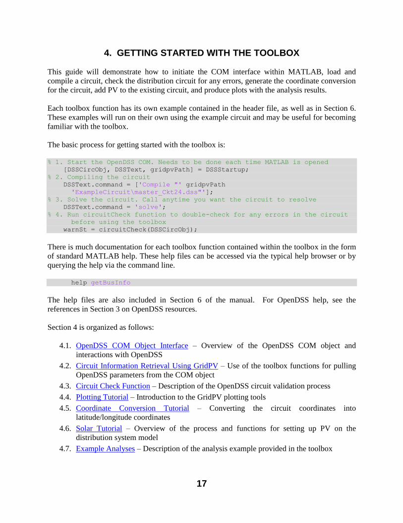
4. GETTING STARTED WITH THE TOOLBOX
This guide will demonstrate how to initiate the COM interface within MATLAB, load and
compile a circuit, check the distribution circuit for any errors, generate the coordinate conversion
for the circuit, add PV to the existing circuit, and produce plots with the analysis results.
Each toolbox function has its own example contained in the header file, as well as in Section 6.
These examples will run on their own using the example circuit and may be useful for becoming
familiar with the toolbox.
The basic process for getting started with the toolbox is:
% 1. Start the OpenDSS COM. Needs to be done each time MATLAB is opened [DSSCircObj, DSSText, gridpvPath] = DSSStartup; % 2. Compiling the circuit DSSText.command = ['Compile "' gridpvPath
'ExampleCircuit\master_Ckt24.dss"']; % 3. Solve the circuit. Call anytime you want the circuit to resolve DSSText.command = 'solve'; % 4. Run circuitCheck function to double-check for any errors in the circuit
before using the toolbox warnSt = circuitCheck(DSSCircObj);
There is much documentation for each toolbox function contained within the toolbox in the form
of standard MATLAB help. These help files can be accessed via the typical help browser or by
querying the help via the command line.
help getBusInfo
The help files are also included in Section 6 of the manual. For OpenDSS help, see the
references in Section 3 on OpenDSS resources.
Section 4 is organized as follows:
4.1. OpenDSS COM Object Interface – Overview of the OpenDSS COM object and
interactions with OpenDSS
4.2. Circuit Information Retrieval Using GridPV – Use of the toolbox functions for pulling
OpenDSS parameters from the COM object
4.3. Circuit Check Function – Description of the OpenDSS circuit validation process
4.4. Plotting Tutorial – Introduction to the GridPV plotting tools
4.5. Coordinate Conversion Tutorial – Converting the circuit coordinates into
latitude/longitude coordinates
4.6. Solar Tutorial – Overview of the process and functions for setting up PV on the
distribution system model
4.7. Example Analyses – Description of the analysis example provided in the toolbox
18
4.1. OpenDSS COM Object Interface
This section provides an overview of the interaction between MATLAB and OpenDSS through
the COM server object. The features and methods described in Section 4.1 are built in to the
OpenDSS COM server and can be accessed from other programs such as VBA in Excel. The
purpose is to give the reader a basic understanding of the OpenDSS COM, and further
information about the OpenDSS COM server can be found in the OpenDSS resources in Section
3.
4.1.1. Initiating the COM Interface
The first step is to initiate the COM interface. A MATLAB function in the toolbox does this for
the user by calling DSSStartup:
[DSSCircObj, DSSText, gridpvPath] = DSSStartup;
DSSStartup starts up OpenDSS in the background and returns the handle pointer to MATLAB
for interface. DSSStartup returns three outputs:
DSSCircObj, which is the pointer to the COM interface. This contains the active circuit
(DSSCircObj.ActiveCircuit), which is not yet compiled, and the text interface to
OpenDSS (DSSCircObj.Text). DSSCircObj will be empty until a circuit is compiled, as
discussed in Section 4.1.2 Compiling the Circuit.
DSSText is the text interface contained within DSSCircObj. It has been redefined in this
manner for easier use within the MATLAB command window.
DSSCircObj.Text.Command and Text.command point to the same text interface, except
the latter requires less typing.
gridpvPath is a string containing the toolbox path location on your computer.
DSSStartup will return an error if MATLAB was unable to create a link to OpenDSS. The most
common reasons for this error are if OpenDSS is not installed on the computer or if an older
version of OpenDSS was installed.
Note that the OpenDSS program that MATLAB interfaces with via the COM server is different
than the graphical interface window of the OpenDSS executable. Any information, circuits,
solutions, or parameters set in the graphical interface window of OpenDSS will not show up in
the COM server version of OpenDSS, and vice versa.
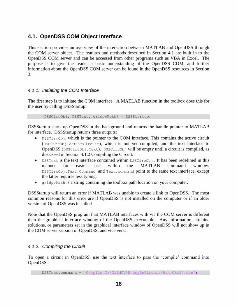
4.1.2. Compiling the Circuit
To open a circuit in OpenDSS, use the text interface to pass the ‘compile’ command into
OpenDSS. DSSText.command = 'Compile C:\GridPV\ExampleCircuit\Run_Ckt24.dss';

19
Relative file paths can be used in the compile command, but the OpenDSS directory will change
to the folder that contains the .dss file during the compile command. To ensure that the compile
command works every time, it is recommended to use the full file path.
When working with the example circuit in the toolbox, the gridpvPath returned from
DSSStartup can be used to link to the circuit. For example, use
DSSText.command = ['Compile "', gridpvPath,
'ExampleCircuit\master_Ckt24.dss"'];
IMPORTANT NOTE: At this point you have opened an instance of OpenDSS in the background
and compiled a circuit. This instance of OpenDSS is entirely unassociated with any visible
instance of OpenDSS (the GUI) that you may already have open. Changes to a circuit in the
OpenDSS GUI will not be reflected in the MATLAB OpenDSS circuit.
To make changes to the circuit, use either the DSSText interface inside MATLAB. Alternatively,
manually edit the .dss files, save them, and recompile the circuit in MATLAB.
4.1.3. Getting Data into MATLAB from OpenDSS
Now that the COM interface has been started and the circuit has been solved, you can begin to
use the Command Window to interact with the COM interface structure.
Call DSSCircObj.methods to view the available methods with which you can use to interact
with the interface. Use the DSSCircObj.get method to view the main interface. For information
on the rest of the methods, refer to OpenDSS documentation and resources in Section 3.
In the return for DSSCircObj.get, notice that there are several other pointers to OpenDSS
interface COM objects. One such sub-pointer is the ActiveCircuit interface. The ActiveCircuit
refers to the compiled circuit in OpenDSS and contains all parameters and power flow solutions.
Since the ActiveCircuit pointer will be used regularly, redefining the active circuit interface as its
own, separate handle can save on the amount of typing in the future:
DSSCircuit = DSSCircObj.ActiveCircuit;
Now call DSSCircuit.methods to view the methods pertaining to the solved circuit. Again, use
the DSSCircuit.get method to view all the different fields and interfaces present in the circuit
interface:
DSSCircuit.methods
DSSCircuit.get
In the return after calling DSSCircuit.get, you will notice several more OpenDSS COM
interface pointers, each referring to specific elements in the circuit. You can also view the
methods of any of these interfaces that appear as fields of DSSCircuit. Notice the fields that

20
show up in the return. Now that you are aware of what the lines interface contains, you can query
a specific field.
DSSCircuit.Lines.methods
DSSCircuit.Lines.get
DSSCircuit.Lines.LineCode
DSSCircuit.Capacitors.get
DSSCircuit.Capacitors.Name
However, you should also notice that most of these fields in these interfaces are populated with
information about an individual line. The fields refer to data about the element that you are
currently viewing, which is initially the first element by default.
This is an important observation to understanding how iteration is used to retrieve all the data
about a circuit. The .first and .next methods that were present in the return for
DSSCircuit.Lines.get are used to change the index of the object. Use the .first method to
be certain that you have reset the current line, capacitor, etc. to the first one in the list. Then, use
the .next method while iterating to step through the list. This is true for each type of circuit
element present in the OpenDSS COM, such as Lines, Capacitors, Transformers, etc.
% Set transformer element to beginning DSSCircuit.Transformers.first; % Get total number of transformers numXfmr = DSSCircuit.Transformers.count; % Preallocate xfmrNames = cell(numXfmr, 1); % Iterate for ii = 1:numXfmr %Get current transformer name xfmrNames{ii} = DSSCircuit.Transformers.Name; % Advance to next transformer DSSCircuit.Transformers.Next;
end
Notice the use of the numXfmr variable. Initially, it may seem useful to save this line of code and
just use DSSCircuit.Transformers.count in the two locations that numXfmr appears.
However, DSSCircuit.Transformers.count has to go through the COM server and takes more
time; therefore, it is most efficient to call this just once and then use the workspace variable
going forward.
The above transformer example is solely for demonstration of using iteration with the interfaces.
It is not the easiest way to obtain all of the transformer names. This highlights another point
about these element interfaces: even though many of the fields will be specific to a single
element, there are several methods and fields that return or contain global information. Be sure to
look over what methods and fields are available, as they can save resources by avoiding iteration.
Notice that the following method is effectively the same as the above loop:
xfmrNames = DSSCircuit.Transformers.AllNames;
21
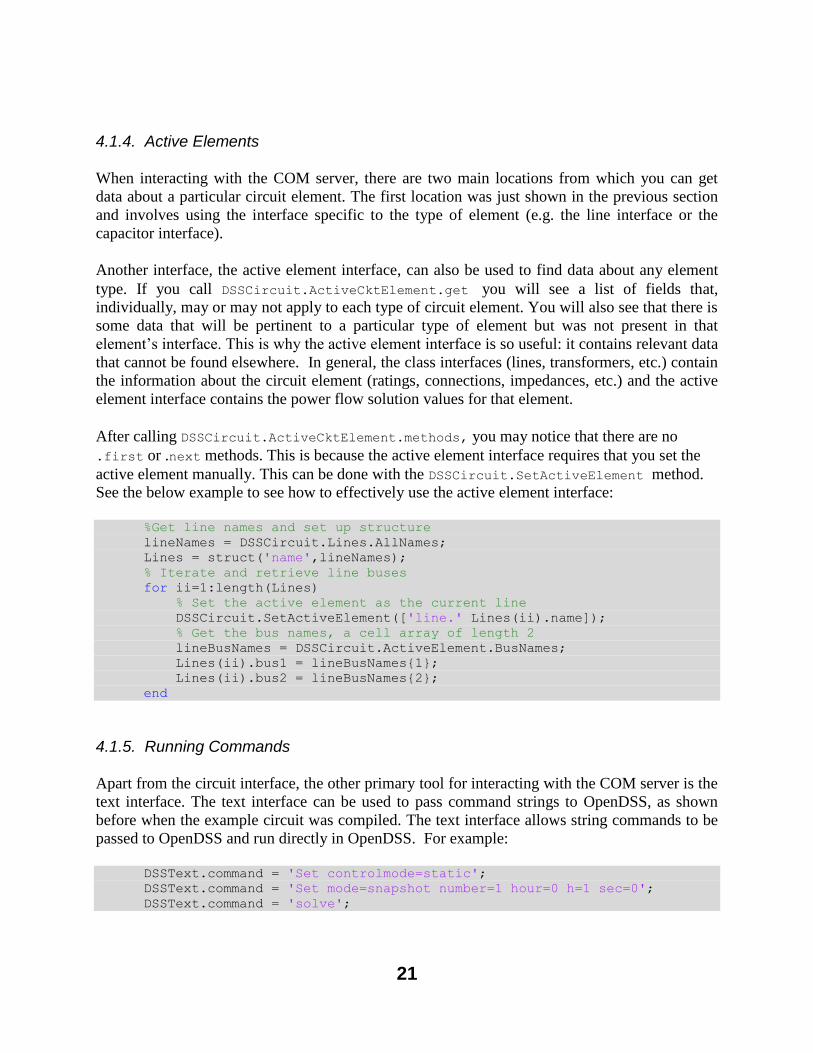
4.1.4. Active Elements
When interacting with the COM server, there are two main locations from which you can get
data about a particular circuit element. The first location was just shown in the previous section
and involves using the interface specific to the type of element (e.g. the line interface or the
capacitor interface).
Another interface, the active element interface, can also be used to find data about any element
type. If you call DSSCircuit.ActiveCktElement.get you will see a list of fields that,
individually, may or may not apply to each type of circuit element. You will also see that there is
some data that will be pertinent to a particular type of element but was not present in that
element’s interface. This is why the active element interface is so useful: it contains relevant data
that cannot be found elsewhere. In general, the class interfaces (lines, transformers, etc.) contain
the information about the circuit element (ratings, connections, impedances, etc.) and the active
element interface contains the power flow solution values for that element.
After calling DSSCircuit.ActiveCktElement.methods, you may notice that there are no
.first or .next methods. This is because the active element interface requires that you set the
active element manually. This can be done with the DSSCircuit.SetActiveElement method.
See the below example to see how to effectively use the active element interface:
%Get line names and set up structure
lineNames = DSSCircuit.Lines.AllNames;
Lines = struct('name',lineNames);
% Iterate and retrieve line buses
for ii=1:length(Lines)
% Set the active element as the current line
DSSCircuit.SetActiveElement(['line.' Lines(ii).name]);
% Get the bus names, a cell array of length 2
lineBusNames = DSSCircuit.ActiveElement.BusNames;
Lines(ii).bus1 = lineBusNames{1};
Lines(ii).bus2 = lineBusNames{2};
end
4.1.5. Running Commands
Apart from the circuit interface, the other primary tool for interacting with the COM server is the
text interface. The text interface can be used to pass command strings to OpenDSS, as shown
before when the example circuit was compiled. The text interface allows string commands to be
passed to OpenDSS and run directly in OpenDSS. For example:
DSSText.command = 'Set controlmode=static'; DSSText.command = 'Set mode=snapshot number=1 hour=0 h=1 sec=0'; DSSText.command = 'solve';
22
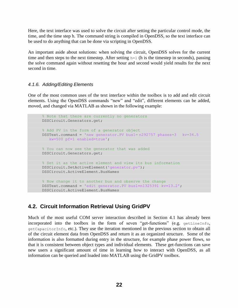
Here, the text interface was used to solve the circuit after setting the particular control mode, the
time, and the time step h. The command string is compiled in OpenDSS, so the text interface can
be used to do anything that can be done via scripting in OpenDSS.
An important aside about solutions: when solving the circuit, OpenDSS solves for the current
time and then steps to the next timestep. After setting h=1 (h is the timestep in seconds), passing
the solve command again without resetting the hour and second would yield results for the next
second in time.
4.1.6. Adding/Editing Elements
One of the most common uses of the text interface within the toolbox is to add and edit circuit
elements. Using the OpenDSS commands “new” and “edit”, different elements can be added,
moved, and changed via MATLAB as shown in the following example:
% Note that there are currently no generators DSSCircuit.Generators.get;
% Add PV in the form of a generator object
DSSText.command = 'new generator.PV bus1= n292757 phases=3 kv=34.5
kw=500 pf=1 enabled=true';
% You can now see the generator that was added DSSCircuit.Generators.get;
% Set it as the active element and view its bus information DSSCircuit.SetActiveElement('generator.pv'); DSSCircuit.ActiveElement.BusNames
% Now change it to another bus and observe the change DSSText.command = 'edit generator.PV bus1=n1325391 kv=13.2'; DSSCircuit.ActiveElement.BusNames
4.2. Circuit Information Retrieval Using GridPV
Much of the most useful COM server interaction described in Section 4.1 has already been
incorporated into the toolbox in the form of seven “get-functions” (e.g. getLineInfo,
getCapacitorInfo, etc.). They use the iteration mentioned in the previous section to obtain all
of the circuit element data from OpenDSS and return it as an organized structure. Some of the
information is also formatted during entry in the structure, for example phase power flows, so
that it is consistent between object types and individual elements. These get-functions can save
new users a significant amount of time in learning how to interact with OpenDSS, as all
information can be queried and loaded into MATLAB using the GridPV toolbox.
23
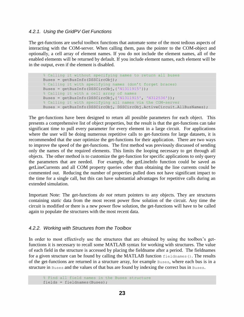
4.2.1. Using the GridPV Get Functions
The get-functions are useful toolbox functions that automate some of the most tedious aspects of
interacting with the COM-server. When calling them, pass the pointer to the COM-object and
optionally, a cell array of element names. If you do not include the element names, all of the
enabled elements will be returned by default. If you include element names, each element will be
in the output, even if the element is disabled.
% Calling it without specifying names to return all buses Buses = getBusInfo(DSSCircObj);
% Calling it with specifying names (don’t forget braces) Buses = getBusInfo(DSSCircObj,{'N1311915'});
% Calling it with a cell array of names Buses = getBusInfo(DSSCircObj,{'N1311915', 'N312536'});
% Calling it with specifying all names via the COM-server Buses = getBusInfo(DSSCircObj, DSSCircObj.ActiveCircuit.AllBusNames);
The get-functions have been designed to return all possible parameters for each object. This
presents a comprehensive list of object properties, but the result is that the get-functions can take
significant time to pull every parameter for every element in a large circuit. For applications
where the user will be doing numerous repetitive calls to get-functions for large datasets, it is
recommended that the user optimize the get-functions for their application. There are two ways
to improve the speed of the get-functions. The first method was previously discussed of sending
only the names of the required elements. This limits the looping necessary to get through all
objects. The other method is to customize the get-function for specific applications to only query
the parameters that are needed. For example, the getLineInfo function could be saved as
getLineCurrents and all COM property queries other than obtaining the line currents could be
commented out. Reducing the number of properties pulled does not have significant impact to
the time for a single call, but this can have substantial advantages for repetitive calls during an
extended simulation.
Important Note: The get-functions do not return pointers to any objects. They are structures
containing static data from the most recent power flow solution of the circuit. Any time the
circuit is modified or there is a new power flow solution, the get-functions will have to be called
again to populate the structures with the most recent data.
4.2.2. Working with Structures from the Toolbox
In order to most effectively use the structures that are obtained by using the toolbox’s get-
functions it is necessary to recall some MATLAB syntax for working with structures. The value
of each field in the structure is accessed by placing the fieldname after a period. The fieldnames
for a given structure can be found by calling the MATLAB function fieldnames(). The results
of the get-functions are returned in a structure array, for example Buses, where each bus is in a
structure in Buses and the values of that bus are found by indexing the correct bus in Buses.
% Find all field names in the Buses structure
fields = fieldnames(Buses);
24
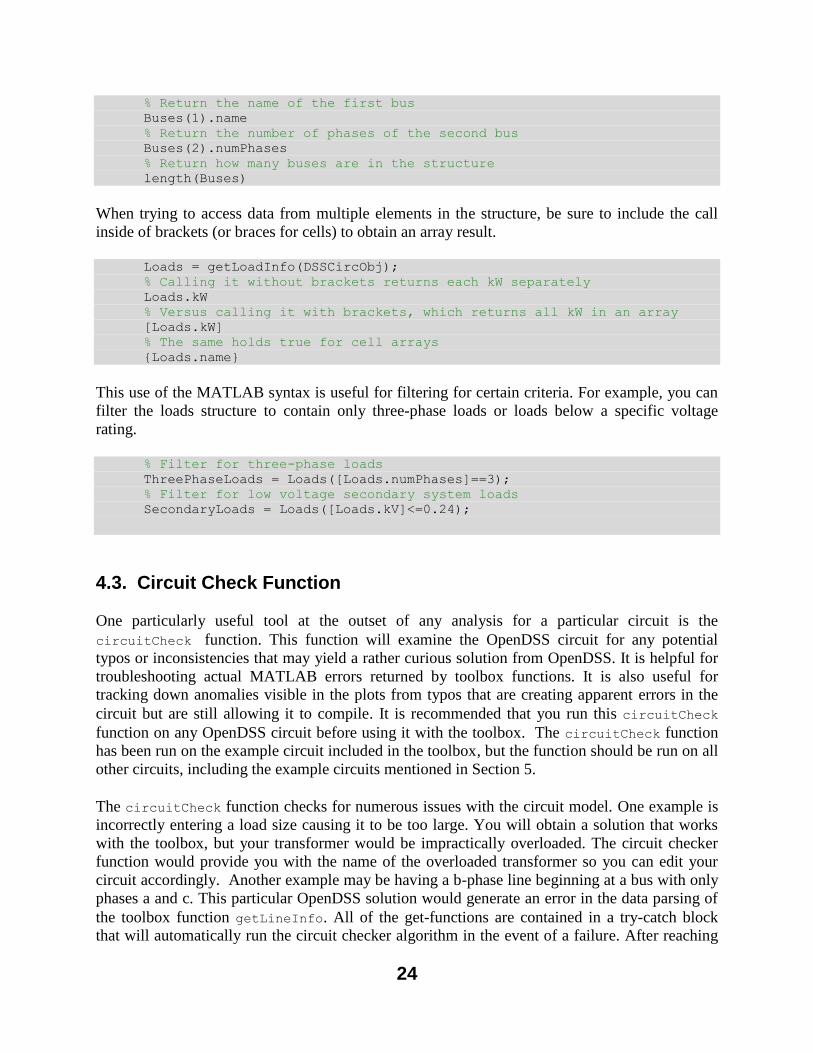
% Return the name of the first bus Buses(1).name % Return the number of phases of the second bus Buses(2).numPhases
% Return how many buses are in the structure length(Buses)
When trying to access data from multiple elements in the structure, be sure to include the call
inside of brackets (or braces for cells) to obtain an array result.
Loads = getLoadInfo(DSSCircObj);
% Calling it without brackets returns each kW separately Loads.kW % Versus calling it with brackets, which returns all kW in an array [Loads.kW] % The same holds true for cell arrays
{Loads.name}
This use of the MATLAB syntax is useful for filtering for certain criteria. For example, you can
filter the loads structure to contain only three-phase loads or loads below a specific voltage
rating.
% Filter for three-phase loads ThreePhaseLoads = Loads([Loads.numPhases]==3);
% Filter for low voltage secondary system loads SecondaryLoads = Loads([Loads.kV]<=0.24);
4.3. Circuit Check Function
One particularly useful tool at the outset of any analysis for a particular circuit is the
circuitCheck function. This function will examine the OpenDSS circuit for any potential
typos or inconsistencies that may yield a rather curious solution from OpenDSS. It is helpful for
troubleshooting actual MATLAB errors returned by toolbox functions. It is also useful for
tracking down anomalies visible in the plots from typos that are creating apparent errors in the
circuit but are still allowing it to compile. It is recommended that you run this circuitCheck
function on any OpenDSS circuit before using it with the toolbox. The circuitCheck function
has been run on the example circuit included in the toolbox, but the function should be run on all
other circuits, including the example circuits mentioned in Section 5.
The circuitCheck function checks for numerous issues with the circuit model. One example is
incorrectly entering a load size causing it to be too large. You will obtain a solution that works
with the toolbox, but your transformer would be impractically overloaded. The circuit checker
function would provide you with the name of the overloaded transformer so you can edit your
circuit accordingly. Another example may be having a b-phase line beginning at a bus with only
phases a and c. This particular OpenDSS solution would generate an error in the data parsing of
the toolbox function getLineInfo. All of the get-functions are contained in a try-catch block
that will automatically run the circuit checker algorithm in the event of a failure. After reaching
25
this error, the toolbox would identify the cause and return the original error along with the circuit
checker result, which would contain the offending line name.
4.3.1. Running Circuit Check Function
To run circuitCheck manually, first compile and solve the circuit. Then, include the pointer to
the COM-object as well as the warning option in a call to circuitCheck. The warnings field is
optional, and the default value is to have warnings on.
warnSt = circuitCheck(DSSCircObj, 'Warnings', 'off');
warnSt = circuitCheck(DSSCircObj);
If warnings are on, the warnSt.str will be printed to the Command Window after completing
the check. Regardless of the warnings setting, the warnSt.offenders will always have to be
accessed via the workspace. Open the warnSt variable from the MATLAB workspace by double
clicking on it and browsing the errors found in the circuit.
The circuitCheck function is automatically called in any of the get-functions if an error is
encountered.
If there are major issues in the circuit, OpenDSS may not be able to return a valid power flow
solution for the circuit. Without a valid power flow solution, circuitCheck will check for
several potential errors, but there are many pieces that cannot be analyzed.
4.3.2. Interpreting Circuit Check Output
With warnings turned on, any issues with the circuit will show as a warning in the Command
Window. Regardless of whether or not warnings are on, circuitCheck will always output a
warning structure. By checking this structure you can view any of warnings caught by the
function. Each element of the structure corresponds to a single warning and will contain a string
describing the warning as well as a list of elements that violate that error-check. After receiving
warnings, you should always check this structure to begin troubleshooting your circuit (or if
warnings are set to off, always check to see whether the output structure is empty).
The default thresholds for each check can be changed by editing the thresholds towards the top
of the circuitCheck.m file.
The purpose of circuitCheck is to identify potential issues. Not every warning returned by
circuitCheck is necessarily something that is wrong with the circuit. The user will have to
inspect the output to determine which of the warnings are actually errors in the circuit that should
be corrected.
The warnings that may be shown are listed below:
26
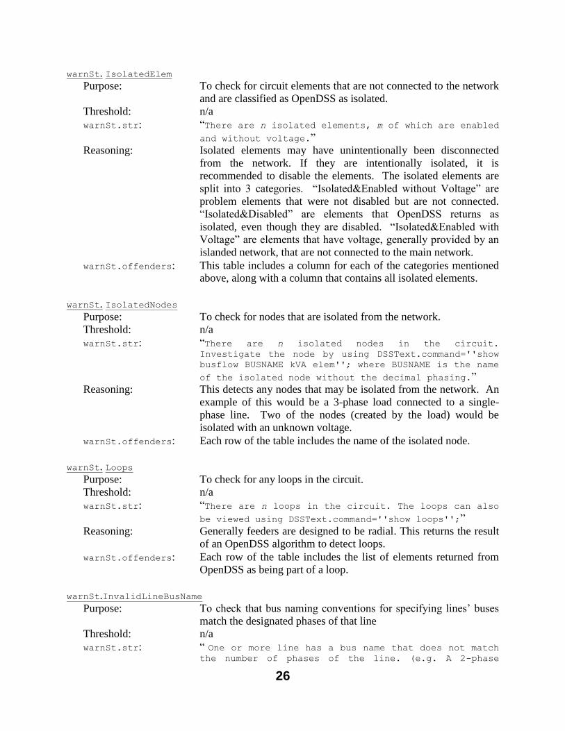
warnSt. IsolatedElem
Purpose: To check for circuit elements that are not connected to the network
and are classified as OpenDSS as isolated.
Threshold: n/a
warnSt.str: “There are n isolated elements, m of which are enabled
and without voltage.”
Reasoning: Isolated elements may have unintentionally been disconnected
from the network. If they are intentionally isolated, it is
recommended to disable the elements. The isolated elements are
split into 3 categories. “Isolated&Enabled without Voltage” are
problem elements that were not disabled but are not connected.
“Isolated&Disabled” are elements that OpenDSS returns as
isolated, even though they are disabled. “Isolated&Enabled with
Voltage” are elements that have voltage, generally provided by an
islanded network, that are not connected to the main network.
warnSt.offenders: This table includes a column for each of the categories mentioned
above, along with a column that contains all isolated elements.
warnSt. IsolatedNodes
Purpose: To check for nodes that are isolated from the network.
Threshold: n/a
warnSt.str: “There are n isolated nodes in the circuit.
Investigate the node by using DSSText.command=''show
busflow BUSNAME kVA elem''; where BUSNAME is the name
of the isolated node without the decimal phasing.”
Reasoning: This detects any nodes that may be isolated from the network. An
example of this would be a 3-phase load connected to a single-
phase line. Two of the nodes (created by the load) would be
isolated with an unknown voltage.
warnSt.offenders: Each row of the table includes the name of the isolated node.
warnSt. Loops
Purpose: To check for any loops in the circuit.
Threshold: n/a
warnSt.str: “There are n loops in the circuit. The loops can also
be viewed using DSSText.command=''show loops'';”
Reasoning: Generally feeders are designed to be radial. This returns the result
of an OpenDSS algorithm to detect loops.
warnSt.offenders: Each row of the table includes the list of elements returned from
OpenDSS as being part of a loop.
warnSt.InvalidLineBusName
Purpose: To check that bus naming conventions for specifying lines’ buses
match the designated phases of that line
Threshold: n/a
warnSt.str: “ One or more line has a bus name that does not match the number of phases of the line. (e.g. A 2-phase
27
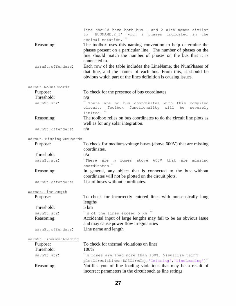
line should have both bus 1 and 2 with names similar
to ‘BUSNAME.2.3’ with 2 phases indicated in the
decimal notation. ”
Reasoning: The toolbox uses this naming convention to help determine the
phases present on a particular line. The number of phases on the
line should match the number of phases on the bus that it is
connected to.
warnSt.offenders: Each row of the table includes the LineName, the NumPhases of
that line, and the names of each bus. From this, it should be
obvious which part of the lines definition is causing issues.
warnSt.NoBusCoords
Purpose: To check for the presence of bus coordinates
Threshold: n/a
warnSt.str: “ There are no bus coordinates with this compiled
circuit. Toolbox functionality will be severely
limited. ”
Reasoning: The toolbox relies on bus coordinates to do the circuit line plots as
well as for any solar integration.
warnSt.offenders: n/a
warnSt. MissingBusCoords
Purpose: To check for medium-voltage buses (above 600V) that are missing
coordinates.
Threshold: n/a
warnSt.str: “There are n buses above 600V that are missing
coordinates.”
Reasoning: In general, any object that is connected to the bus without
coordinates will not be plotted on the circuit plots.
warnSt.offenders: List of buses without coordinates.
warnSt.LineLength
Purpose: To check for incorrectly entered lines with nonsensically long
lengths
Threshold: 5 km
warnSt.str: “ n of the lines exceed 5 km. ”
Reasoning: Accidental input of large lengths may fail to be an obvious issue
and may cause power flow irregularities
warnSt.offenders: Line name and length
warnSt.LineOverLoading
Purpose: To check for thermal violations on lines
Threshold: 100%
warnSt.str: “ n Lines are load more than 100%. Visualize using
plotCircuitLines(DSSCircObj,'Coloring','lineLoading')”
Reasoning: Notifies you of line loading violations that may be a result of
incorrect parameters in the circuit such as line ratings
28
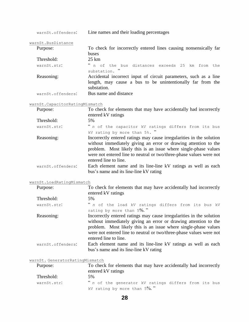
warnSt.offenders: Line names and their loading percentages
warnSt.BusDistance
Purpose: To check for incorrectly entered lines causing nonsensically far
buses
Threshold: 25 km
warnSt.str: “ n of the bus distances exceeds 25 km from the
substation. ”
Reasoning: Accidental incorrect input of circuit parameters, such as a line
length, may cause a bus to be unintentionally far from the
substation.
warnSt.offenders: Bus name and distance
warnSt.CapacitorRatingMismatch
Purpose: To check for elements that may have accidentally had incorrectly
entered kV ratings
Threshold: 5%
warnSt.str: “ n of the capacitor kV ratings differs from its bus
kV rating by more than 5%. ”
Reasoning: Incorrectly entered ratings may cause irregularities in the solution
without immediately giving an error or drawing attention to the
problem. Most likely this is an issue where single-phase values
were not entered line to neutral or two/three-phase values were not
entered line to line.
warnSt.offenders: Each element name and its line-line kV ratings as well as each
bus’s name and its line-line kV rating
warnSt.LoadRatingMismatch
Purpose: To check for elements that may have accidentally had incorrectly
entered kV ratings
Threshold: 5%
warnSt.str: “ n of the load kV ratings differs from its bus kV
rating by more than 5%. ”
Reasoning: Incorrectly entered ratings may cause irregularities in the solution
without immediately giving an error or drawing attention to the
problem. Most likely this is an issue where single-phase values
were not entered line to neutral or two/three-phase values were not
entered line to line.
warnSt.offenders: Each element name and its line-line kV ratings as well as each
bus’s name and its line-line kV rating
warnSt. GeneratorRatingMismatch
Purpose: To check for elements that may have accidentally had incorrectly
entered kV ratings
Threshold: 5%
warnSt.str: “ n of the generator kV ratings differs from its bus
kV rating by more than 5%. ”
29
Reasoning: Incorrectly entered ratings may cause irregularities in the solution
without immediately giving an error or drawing attention to the
problem. Most likely this is an issue where single-phase values
were not entered line to neutral or two/three-phase values were not
entered line to line.
warnSt.offenders: Each element name and its line-line kV ratings as well as each
bus’s name and its line-line kV rating
warnSt.PVRatingMismatch
Purpose: To check for elements that may have accidentally had incorrectly
entered kV ratings
Threshold: 5%
warnSt.str: “ n of the PV kV ratings differs from its bus kV
rating by more than 5%. ”
Reasoning: Incorrectly entered ratings may cause irregularities in the solution
without immediately giving an error or drawing attention to the
problem. Most likely this is an issue where single-phase values
were not entered line to neutral or two/three-phase values were not
entered line to line.
warnSt.offenders: Each element name and its line-line kV ratings as well as each
bus’s name and its line-line kV rating
warnSt.TransformerRatingMismatch
Purpose: To check for elements that may have accidentally had incorrectly
entered kV ratings on either side of the transformer
Threshold: 5%
warnSt.str: “ n of the transformer kV ratings differs from its bus
kV rating by more than 5%. ”
Reasoning: Incorrectly entered ratings may cause irregularities in the solution
without immediately giving an error or drawing attention to the
problem. Most likely this is an issue where single-phase values
were not entered line to neutral or two/three-phase values were not
entered line to line.
warnSt.offenders: Each element name and its line-line kV ratings as well as each
bus’s name and its line-line kV rating
warnSt.TransformerOverloaded
Purpose: To check for thermal violations on the transformers
Threshold: 5%
warnSt.str: “ n of the transformer kVA ratings differs from its bus1 power by more than %. Check that the loads on
the transformer are entered correctly. ”
Reasoning: Notifies you of transformer loading violations that may be a result
of incorrect parameters in the circuit
warnSt.offenders: Transformer names and their loading percentages
30
warnSt. TransformerNoLoad
Purpose: To check for transformers that do not have any loads downstream
of them.
Threshold: power flow in transformer less than 1% of the transformer rating
and no loads downstream of the transformer
warnSt.str: “n of the transformer have no load on them. Check that
the loads on that transformer are entered correctly.”
Reasoning: This detects any issues during the load allocation process where
loads were not assigned to a service transformer.
warnSt.offenders: Transformer names and their kVA ratings
warnSt. TransformerLowLoad
Purpose: To check for transformers that do not have much power flowing
through it proportional to its rating.
Threshold: power flow in transformer less than 1% of the transformer rating
warnSt.str: “n of the transformer have less than %d percent power flow of their kVA rating. Check that the loads on
that transformer are entered correctly.”
Reasoning: This detects any issues during the load allocation process where
loads were not assigned to a service transformer.
warnSt.offenders: Transformer names, their kVA ratings, sum of the kW ratings for
all loads downstream of the transformer, and the list of loads
downstream of the transformer.
warnSt.BusVoltage
Purpose: To check for over/under voltage violations
Threshold: 1 +/- 0.05 pu
warnSt.str: “ n of the enabled bus voltages are outside of the range 1+/- 0.05 pu. Visualize using
plotVoltageProfile(DSSCircObj)”
Reasoning: Notifies you of voltage violations that may be a result of incorrect
parameters in the circuit causing large voltage changes
warnSt.offenders: Bus name and voltage (both pu and kV) along with rated kV
warnSt.LineRatingMismatch
Purpose: To check for elements that may have accidentally had incorrectly
entered line codes
Threshold: 150%
warnSt.str: “ n of the line ratings are 150% the size of the immediately upstream line. Visualize using
plotCircuitLines(DSSCircObj,'Thickness','lineRating')”
Reasoning: Line ratings that increase downstream may be indicative of
incorrectly entered linecodes (or may be by design)
31
warnSt.offenders: The upstream line name (smaller line) and the downstream line
name (larger line), followed by each line respective line rating as
well as each lines respective line code.
4.4. Plotting Tutorial
This section includes an overview of the plotting features in the GridPV toolbox. Many of the
examples are shown for plotCircuitLines, but the descriptions apply to all plotting function
from section 6.3.
It is important to recall the fact that the OpenDSS COM server in MATLAB is an entirely
separate entity from the OpenDSS GUI that you are able to use independently apart from
MATLAB. This means that any circuit that you may have solved and plotted in your OpenDSS
program outside of MATLAB is irrelevant. Furthermore, any changes to a circuit file will only
take affect once the circuit is recompiled.
4.4.1. Plotting Circuits
Generating the plots is relatively straight forward and is fully demonstrated in section 6.3;
however, there are some particularities that are worth mentioning when generating and using the
toolbox plots.
Firstly, the plots that are generated are representative of the most recent time step power flow
solution. When in doubt, reset the time step to the specific time of interest:
DSSText.command = 'Set mode=duty number=10 hour=13 h=1 sec=1800'; DSSText.command = 'Set controlmode = static'; DSSText.command = 'solve';
figure; plotCircuitLines(DSSCircObj);
As stated in section 6, calling plotCircuitLines in this manner without assigning any property
values will default to opening the GUI by calling plotCircuitLinesOptions.
plotCircuitLinesOptions is the function associated with the GUI and can also be called on its
own in the same manner; however, it does not accept and other parameters.
figure; plotCircuitLinesOptions(DSSCircObj);
It is also possible to call plotCircuitLines with any number of possible parameters described
in Section 6.3.2.
figure;
plotCircuitLines(DSSCircObj,'Coloring','PerPhase','Thickness',3,'Mappin
gBackground','hybrid');
The plotting functions use the MATLAB parameter name and value argument pair notation for
all input options after the handle to the DSSCircObj. If you are unfamiliar with this method of
32
passing parameters into a MATLAB function, note that while the order of specific options does
not matter, each option requires a pair of inputs: the string denoting which option you are about
to define as well as the corresponding specification for that option. For example, in the line
above, the 'Coloring' parameter is being set to 'PerPhase' and the 'Thickness' parameter
will equal 3.
4.4.2. User Interaction with Plots
Using any of the GridPV plotting functions, there are some user interactions available that make
accessing and viewing the OpenDSS power flow data extremely simple. Any line, transformer,
capacitor, load, or PV system is capable of being left and right clicked.
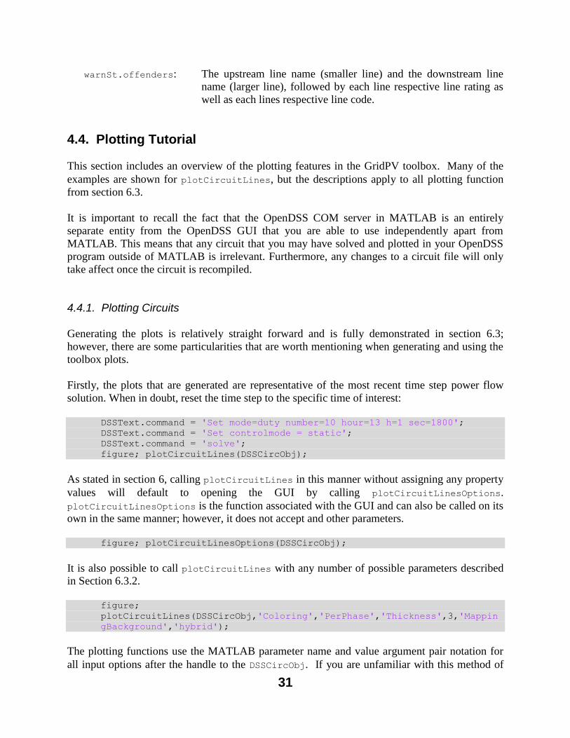
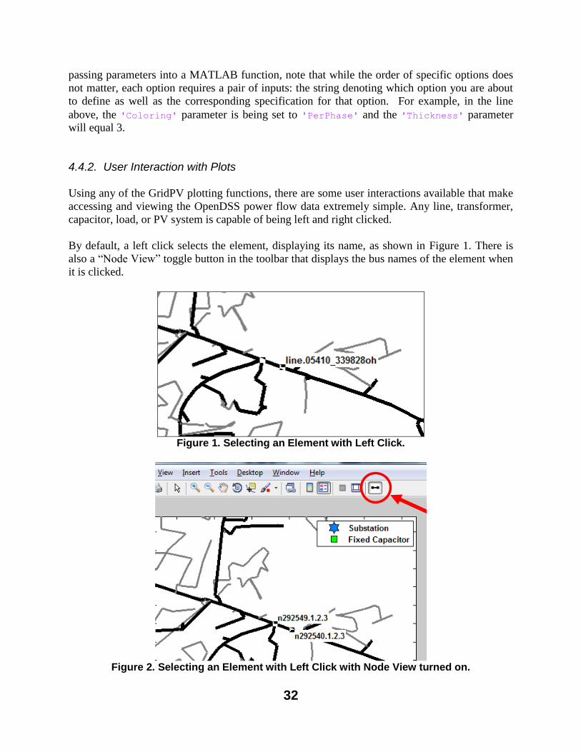
By default, a left click selects the element, displaying its name, as shown in Figure 1. There is
also a “Node View” toggle button in the toolbar that displays the bus names of the element when
it is clicked.
Figure 1. Selecting an Element with Left Click.
Figure 2. Selecting an Element with Left Click with Node View turned on.
33
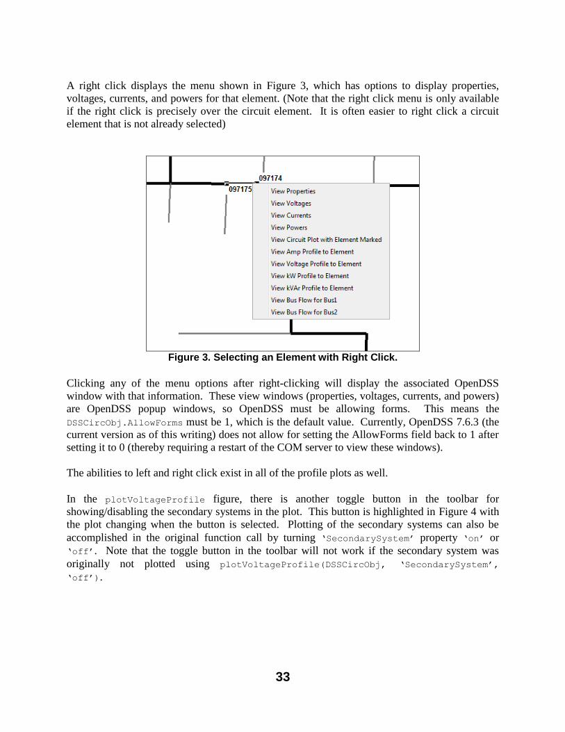
A right click displays the menu shown in Figure 3, which has options to display properties,
voltages, currents, and powers for that element. (Note that the right click menu is only available
if the right click is precisely over the circuit element. It is often easier to right click a circuit
element that is not already selected)
Figure 3. Selecting an Element with Right Click.
Clicking any of the menu options after right-clicking will display the associated OpenDSS
window with that information. These view windows (properties, voltages, currents, and powers)
are OpenDSS popup windows, so OpenDSS must be allowing forms. This means the
DSSCircObj.AllowForms must be 1, which is the default value. Currently, OpenDSS 7.6.3 (the
current version as of this writing) does not allow for setting the AllowForms field back to 1 after
setting it to 0 (thereby requiring a restart of the COM server to view these windows).
The abilities to left and right click exist in all of the profile plots as well.
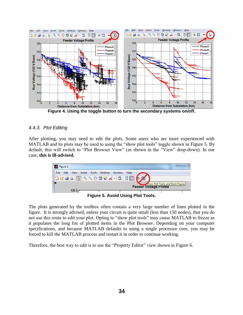
In the plotVoltageProfile figure, there is another toggle button in the toolbar for
showing/disabling the secondary systems in the plot. This button is highlighted in Figure 4 with
the plot changing when the button is selected. Plotting of the secondary systems can also be
accomplished in the original function call by turning ‘SecondarySystem’ property ‘on’ or
‘off’. Note that the toggle button in the toolbar will not work if the secondary system was
originally not plotted using plotVoltageProfile(DSSCircObj, ‘SecondarySystem’,
‘off’).
34
Figure 4. Using the toggle button to turn the secondary systems on/off.
4.4.3. Plot Editing
After plotting, you may need to edit the plots. Some users who are more experienced with
MATLAB and its plots may be used to using the “show plot tools” toggle shown in Figure 5. By
default, this will switch to “Plot Browser View” (as shown in the “View” drop-down). In our
case, this is ill-advised.
Figure 5. Avoid Using Plot Tools.
The plots generated by the toolbox often contain a very large number of lines plotted in the
figure. It is strongly advised, unless your circuit is quite small (less than 150 nodes), that you do
not use this route to edit your plot. Opting to “show plot tools” may cause MATLAB to freeze as
it populates the long list of plotted items in the Plot Browser. Depending on your computer
specifications, and because MATLAB defaults to using a single processor core, you may be
forced to kill the MATLAB process and restart it in order to continue working.
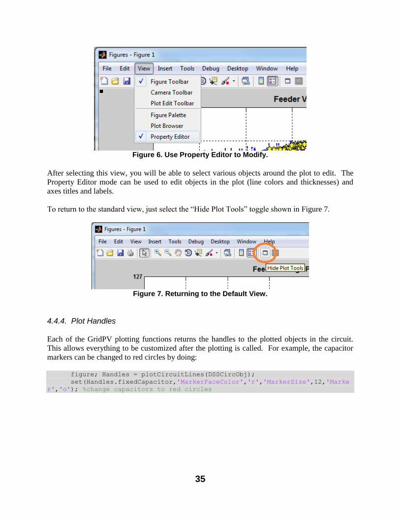
Therefore, the best way to edit is to use the “Property Editor” view shown in Figure 6.
35
Figure 6. Use Property Editor to Modify.
After selecting this view, you will be able to select various objects around the plot to edit. The
Property Editor mode can be used to edit objects in the plot (line colors and thicknesses) and
axes titles and labels.
To return to the standard view, just select the “Hide Plot Tools” toggle shown in Figure 7.
Figure 7. Returning to the Default View.
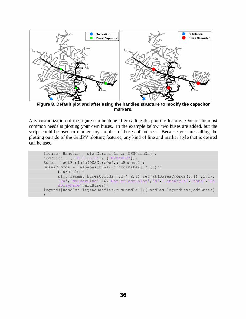
4.4.4. Plot Handles
Each of the GridPV plotting functions returns the handles to the plotted objects in the circuit.
This allows everything to be customized after the plotting is called. For example, the capacitor
markers can be changed to red circles by doing:
figure; Handles = plotCircuitLines(DSSCircObj);
set(Handles.fixedCapacitor,'MarkerFaceColor','r','MarkerSize',12,'Marke
r','o'); %change capacitors to red circles
36
Substation
Fixed Capacitor
Substation
Fixed Capacitor
Figure 8. Default plot and after using the handles structure to modify the capacitor
markers.
Any customization of the figure can be done after calling the plotting feature. One of the most
common needs is plotting your own buses. In the example below, two buses are added, but the
script could be used to marker any number of buses of interest. Because you are calling the
plotting outside of the GridPV plotting features, any kind of line and marker style that is desired
can be used.
figure; Handles = plotCircuitLines(DSSCircObj); addBuses = [{'N1311915'}, {'N284022'}]; Buses = getBusInfo(DSSCircObj,addBuses,1); BusesCoords = reshape([Buses.coordinates],2,[])'; busHandle =
plot(repmat(BusesCoords(:,2)',2,1),repmat(BusesCoords(:,1)',2,1),
'ko','MarkerSize',10,'MarkerFaceColor','c','LineStyle','none','Di
splayName',addBuses); legend([Handles.legendHandles,busHandle'],[Handles.legendText,addBuses]
)
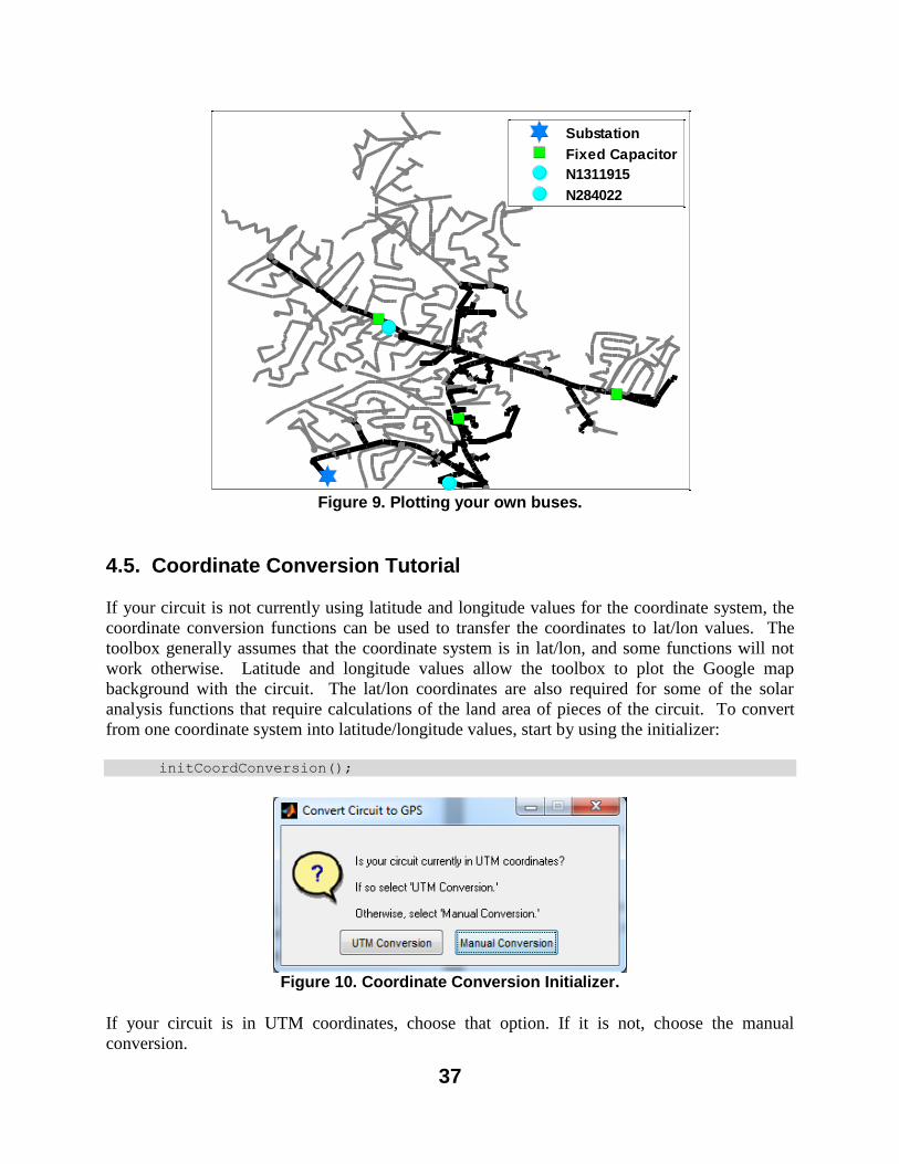
37
Substation
Fixed Capacitor
N1311915
N284022
Figure 9. Plotting your own buses.
4.5. Coordinate Conversion Tutorial
If your circuit is not currently using latitude and longitude values for the coordinate system, the
coordinate conversion functions can be used to transfer the coordinates to lat/lon values. The
toolbox generally assumes that the coordinate system is in lat/lon, and some functions will not
work otherwise. Latitude and longitude values allow the toolbox to plot the Google map
background with the circuit. The lat/lon coordinates are also required for some of the solar
analysis functions that require calculations of the land area of pieces of the circuit. To convert
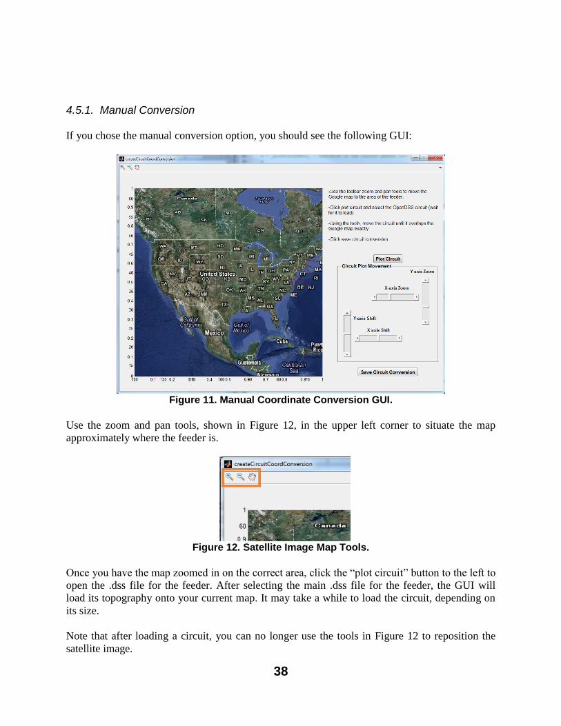
from one coordinate system into latitude/longitude values, start by using the initializer:
initCoordConversion();
Figure 10. Coordinate Conversion Initializer.
If your circuit is in UTM coordinates, choose that option. If it is not, choose the manual
conversion.
38
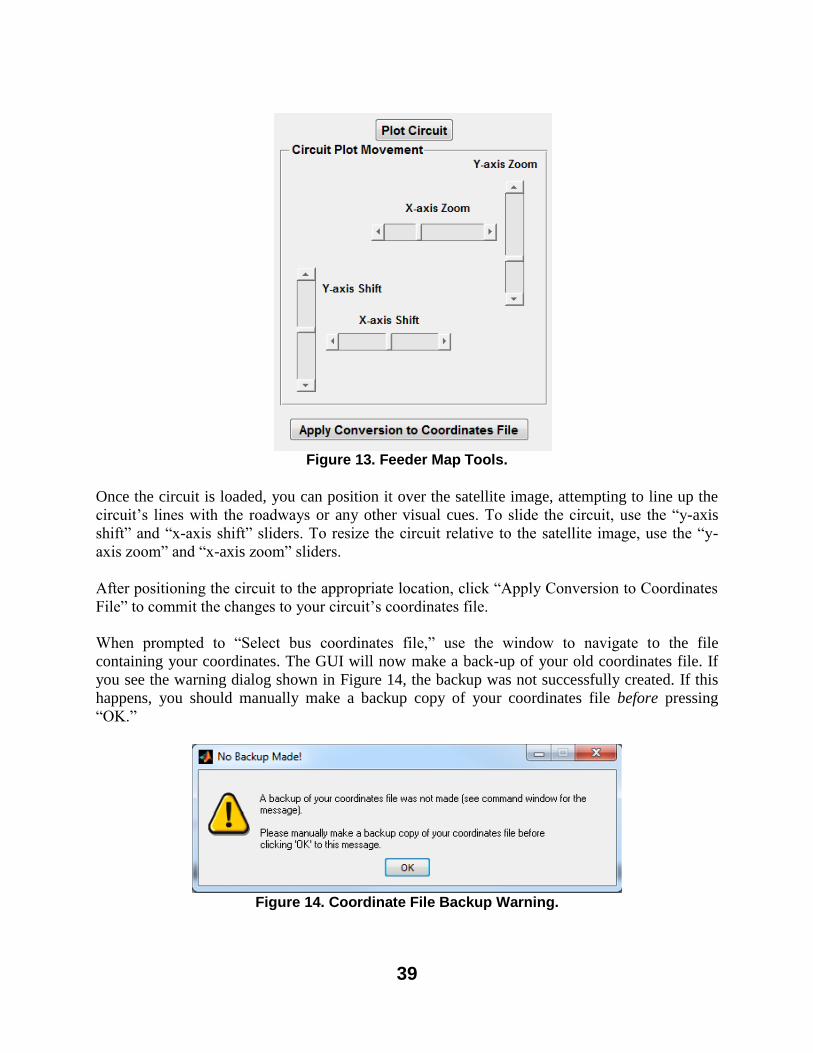
4.5.1. Manual Conversion
If you chose the manual conversion option, you should see the following GUI:
Figure 11. Manual Coordinate Conversion GUI.
Use the zoom and pan tools, shown in Figure 12, in the upper left corner to situate the map
approximately where the feeder is.
Figure 12. Satellite Image Map Tools.
Once you have the map zoomed in on the correct area, click the “plot circuit” button to the left to
open the .dss file for the feeder. After selecting the main .dss file for the feeder, the GUI will
load its topography onto your current map. It may take a while to load the circuit, depending on
its size.
Note that after loading a circuit, you can no longer use the tools in Figure 12 to reposition the
satellite image.
39
Figure 13. Feeder Map Tools.
Once the circuit is loaded, you can position it over the satellite image, attempting to line up the
circuit’s lines with the roadways or any other visual cues. To slide the circuit, use the “y-axis
shift” and “x-axis shift” sliders. To resize the circuit relative to the satellite image, use the “y-
axis zoom” and “x-axis zoom” sliders.
After positioning the circuit to the appropriate location, click “Apply Conversion to Coordinates
File” to commit the changes to your circuit’s coordinates file.
When prompted to “Select bus coordinates file,” use the window to navigate to the file
containing your coordinates. The GUI will now make a back-up of your old coordinates file. If
you see the warning dialog shown in Figure 14, the backup was not successfully created. If this
happens, you should manually make a backup copy of your coordinates file before pressing
“OK.”
Figure 14. Coordinate File Backup Warning.
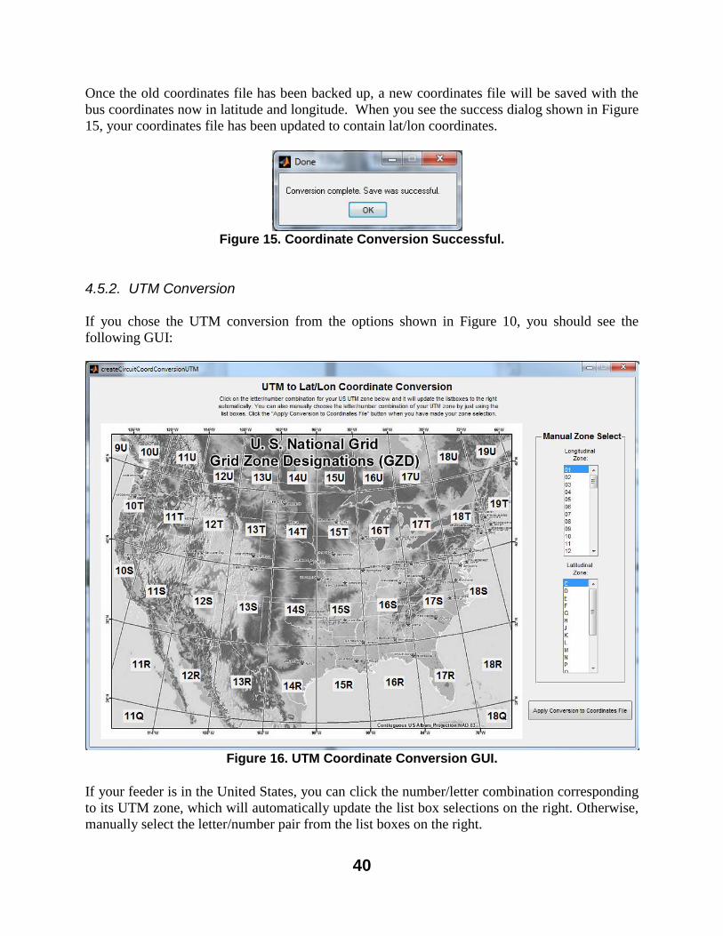
40
Once the old coordinates file has been backed up, a new coordinates file will be saved with the
bus coordinates now in latitude and longitude. When you see the success dialog shown in Figure
15, your coordinates file has been updated to contain lat/lon coordinates.
Figure 15. Coordinate Conversion Successful.
4.5.2. UTM Conversion
If you chose the UTM conversion from the options shown in Figure 10, you should see the
following GUI:
Figure 16. UTM Coordinate Conversion GUI.
If your feeder is in the United States, you can click the number/letter combination corresponding
to its UTM zone, which will automatically update the list box selections on the right. Otherwise,
manually select the letter/number pair from the list boxes on the right.
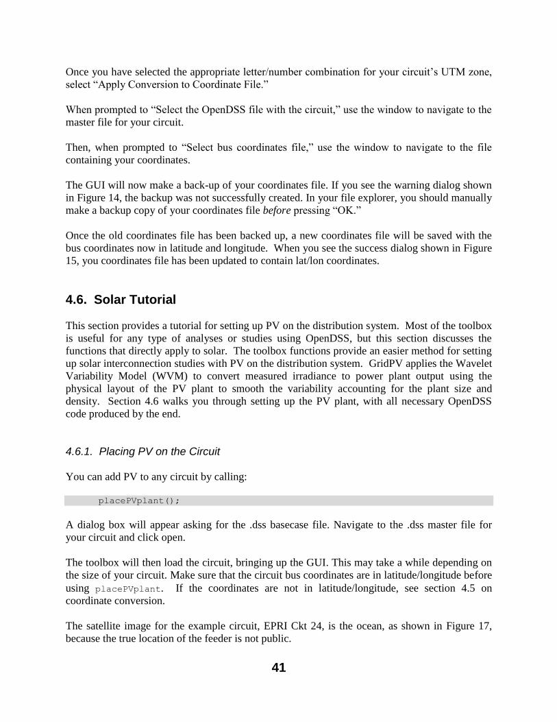
41
Once you have selected the appropriate letter/number combination for your circuit’s UTM zone,
select “Apply Conversion to Coordinate File.”
When prompted to “Select the OpenDSS file with the circuit,” use the window to navigate to the
master file for your circuit.
Then, when prompted to “Select bus coordinates file,” use the window to navigate to the file
containing your coordinates.
The GUI will now make a back-up of your coordinates file. If you see the warning dialog shown
in Figure 14, the backup was not successfully created. In your file explorer, you should manually
make a backup copy of your coordinates file before pressing “OK.”
Once the old coordinates file has been backed up, a new coordinates file will be saved with the
bus coordinates now in latitude and longitude. When you see the success dialog shown in Figure
15, you coordinates file has been updated to contain lat/lon coordinates.
4.6. Solar Tutorial
This section provides a tutorial for setting up PV on the distribution system. Most of the toolbox
is useful for any type of analyses or studies using OpenDSS, but this section discusses the
functions that directly apply to solar. The toolbox functions provide an easier method for setting
up solar interconnection studies with PV on the distribution system. GridPV applies the Wavelet
Variability Model (WVM) to convert measured irradiance to power plant output using the
physical layout of the PV plant to smooth the variability accounting for the plant size and
density. Section 4.6 walks you through setting up the PV plant, with all necessary OpenDSS
code produced by the end.
4.6.1. Placing PV on the Circuit
You can add PV to any circuit by calling:
placePVplant();
A dialog box will appear asking for the .dss basecase file. Navigate to the .dss master file for
your circuit and click open.
The toolbox will then load the circuit, bringing up the GUI. This may take a while depending on
the size of your circuit. Make sure that the circuit bus coordinates are in latitude/longitude before
using placePVplant. If the coordinates are not in latitude/longitude, see section 4.5 on
coordinate conversion.
The satellite image for the example circuit, EPRI Ckt 24, is the ocean, as shown in Figure 17,
because the true location of the feeder is not public.
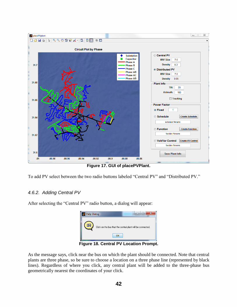
42
Figure 17. GUI of placePVPlant.
To add PV select between the two radio buttons labeled “Central PV” and “Distributed PV.”
4.6.2. Adding Central PV
After selecting the “Central PV” radio button, a dialog will appear:
Figure 18. Central PV Location Prompt.
As the message says, click near the bus on which the plant should be connected. Note that central
plants are three phase, so be sure to choose a location on a three phase line (represented by black
lines). Regardless of where you click, any central plant will be added to the three-phase bus
geometrically nearest the coordinates of your click.
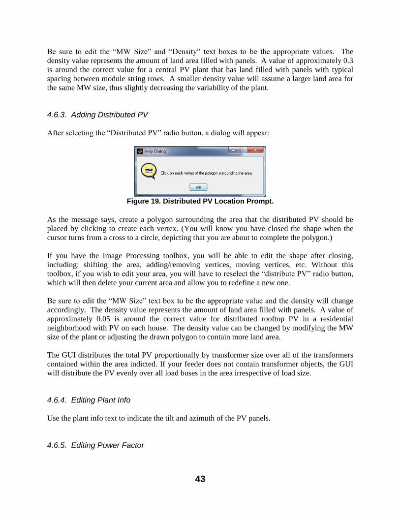
43
Be sure to edit the “MW Size” and “Density” text boxes to be the appropriate values. The
density value represents the amount of land area filled with panels. A value of approximately 0.3
is around the correct value for a central PV plant that has land filled with panels with typical
spacing between module string rows. A smaller density value will assume a larger land area for
the same MW size, thus slightly decreasing the variability of the plant.
4.6.3. Adding Distributed PV
After selecting the “Distributed PV” radio button, a dialog will appear:
Figure 19. Distributed PV Location Prompt.
As the message says, create a polygon surrounding the area that the distributed PV should be
placed by clicking to create each vertex. (You will know you have closed the shape when the
cursor turns from a cross to a circle, depicting that you are about to complete the polygon.)
If you have the Image Processing toolbox, you will be able to edit the shape after closing,
including: shifting the area, adding/removing vertices, moving vertices, etc. Without this
toolbox, if you wish to edit your area, you will have to reselect the “distribute PV” radio button,
which will then delete your current area and allow you to redefine a new one.
Be sure to edit the “MW Size” text box to be the appropriate value and the density will change
accordingly. The density value represents the amount of land area filled with panels. A value of
approximately 0.05 is around the correct value for distributed rooftop PV in a residential
neighborhood with PV on each house. The density value can be changed by modifying the MW
size of the plant or adjusting the drawn polygon to contain more land area.
The GUI distributes the total PV proportionally by transformer size over all of the transformers
contained within the area indicted. If your feeder does not contain transformer objects, the GUI
will distribute the PV evenly over all load buses in the area irrespective of load size.
4.6.4. Editing Plant Info
Use the plant info text to indicate the tilt and azimuth of the PV panels.
4.6.5. Editing Power Factor
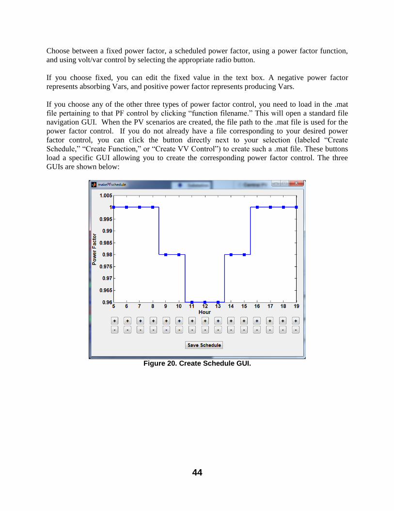
44
Choose between a fixed power factor, a scheduled power factor, using a power factor function,
and using volt/var control by selecting the appropriate radio button.
If you choose fixed, you can edit the fixed value in the text box. A negative power factor
represents absorbing Vars, and positive power factor represents producing Vars.
If you choose any of the other three types of power factor control, you need to load in the .mat
file pertaining to that PF control by clicking “function filename.” This will open a standard file
navigation GUI. When the PV scenarios are created, the file path to the .mat file is used for the
power factor control. If you do not already have a file corresponding to your desired power
factor control, you can click the button directly next to your selection (labeled “Create
Schedule,” “Create Function,” or “Create VV Control”) to create such a .mat file. These buttons
load a specific GUI allowing you to create the corresponding power factor control. The three
GUIs are shown below:
Figure 20. Create Schedule GUI.
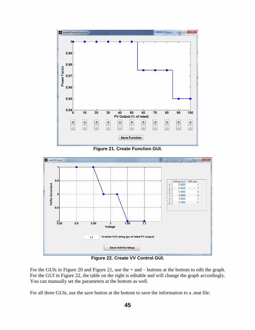
45
Figure 21. Create Function GUI.
Figure 22. Create VV Control GUI.
For the GUIs in Figure 20 and Figure 21, use the + and – buttons at the bottom to edit the graph.
For the GUI in Figure 22, the table on the right is editable and will change the graph accordingly.
You can manually set the parameters at the bottom as well.
For all three GUIs, use the save button at the bottom to save the information to a .mat file.
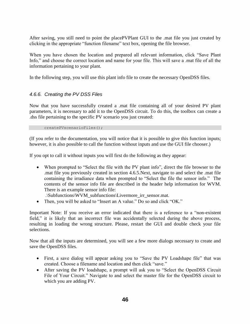
46
After saving, you still need to point the placePVPlant GUI to the .mat file you just created by
clicking in the appropriate “function filename” text box, opening the file browser.
When you have chosen the location and prepared all relevant information, click “Save Plant
Info,” and choose the correct location and name for your file. This will save a .mat file of all the
information pertaining to your plant.
In the following step, you will use this plant info file to create the necessary OpenDSS files.
4.6.6. Creating the PV DSS Files
Now that you have successfully created a .mat file containing all of your desired PV plant
parameters, it is necessary to add it to the OpenDSS circuit. To do this, the toolbox can create a
.dss file pertaining to the specific PV scenario you just created:
createPVscenarioFiles();
(If you refer to the documentation, you will notice that it is possible to give this function inputs;
however, it is also possible to call the function without inputs and use the GUI file chooser.)
If you opt to call it without inputs you will first do the following as they appear:
When prompted to “Select the file with the PV plant info”, direct the file browser to the
.mat file you previously created in section 4.6.5.Next, navigate to and select the .mat file
containing the irradiance data when prompted to “Select the file the sensor info.” The
contents of the sensor info file are described in the header help information for WVM.
There is an example sensor info file:
.\Subfunctions\WVM_subfunctions\Livermore_irr_sensor.mat.
Then, you will be asked to “Insert an A value.” Do so and click “OK.”
Important Note: If you receive an error indicated that there is a reference to a “non-existent
field,” it is likely that an incorrect file was accidentally selected during the above process,
resulting in loading the wrong structure. Please, restart the GUI and double check your file
selections.
Now that all the inputs are determined, you will see a few more dialogs necessary to create and
save the OpenDSS files.
First, a save dialog will appear asking you to “Save the PV Loadshape file” that was
created. Choose a filename and location and then click “save.”
After saving the PV loadshape, a prompt will ask you to “Select the OpenDSS Circuit
File of Your Circuit.” Navigate to and select the master file for the OpenDSS circuit to
which you are adding PV.
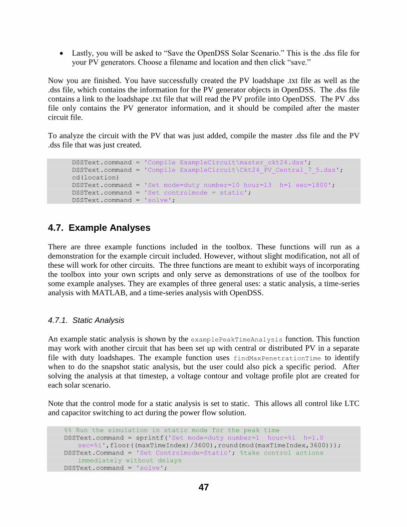
47
Lastly, you will be asked to “Save the OpenDSS Solar Scenario.” This is the .dss file for
your PV generators. Choose a filename and location and then click “save.”
Now you are finished. You have successfully created the PV loadshape .txt file as well as the
.dss file, which contains the information for the PV generator objects in OpenDSS. The .dss file
contains a link to the loadshape .txt file that will read the PV profile into OpenDSS. The PV .dss
file only contains the PV generator information, and it should be compiled after the master
circuit file.
To analyze the circuit with the PV that was just added, compile the master .dss file and the PV
.dss file that was just created.
DSSText.command = 'Compile ExampleCircuit\master_ckt24.dss'; DSSText.command = 'Compile ExampleCircuit\Ckt24_PV_Central_7_5.dss'; cd(location) DSSText.command = 'Set mode=duty number=10 hour=13 h=1 sec=1800'; DSSText.command = 'Set controlmode = static'; DSSText.command = 'solve';
4.7. Example Analyses
There are three example functions included in the toolbox. These functions will run as a
demonstration for the example circuit included. However, without slight modification, not all of
these will work for other circuits. The three functions are meant to exhibit ways of incorporating
the toolbox into your own scripts and only serve as demonstrations of use of the toolbox for
some example analyses. They are examples of three general uses: a static analysis, a time-series
analysis with MATLAB, and a time-series analysis with OpenDSS.
4.7.1. Static Analysis
An example static analysis is shown by the examplePeakTimeAnalysis function. This function
may work with another circuit that has been set up with central or distributed PV in a separate
file with duty loadshapes. The example function uses findMaxPenetrationTime to identify
when to do the snapshot static analysis, but the user could also pick a specific period. After
solving the analysis at that timestep, a voltage contour and voltage profile plot are created for
each solar scenario.
Note that the control mode for a static analysis is set to static. This allows all control like LTC
and capacitor switching to act during the power flow solution.
%% Run the simulation in static mode for the peak time DSSText.command = sprintf('Set mode=duty number=1 hour=%i h=1.0
sec=%i',floor((maxTimeIndex)/3600),round(mod(maxTimeIndex,3600))); DSSText.Command = 'Set Controlmode=Static'; %take control actions
immediately without delays DSSText.command = 'solve';
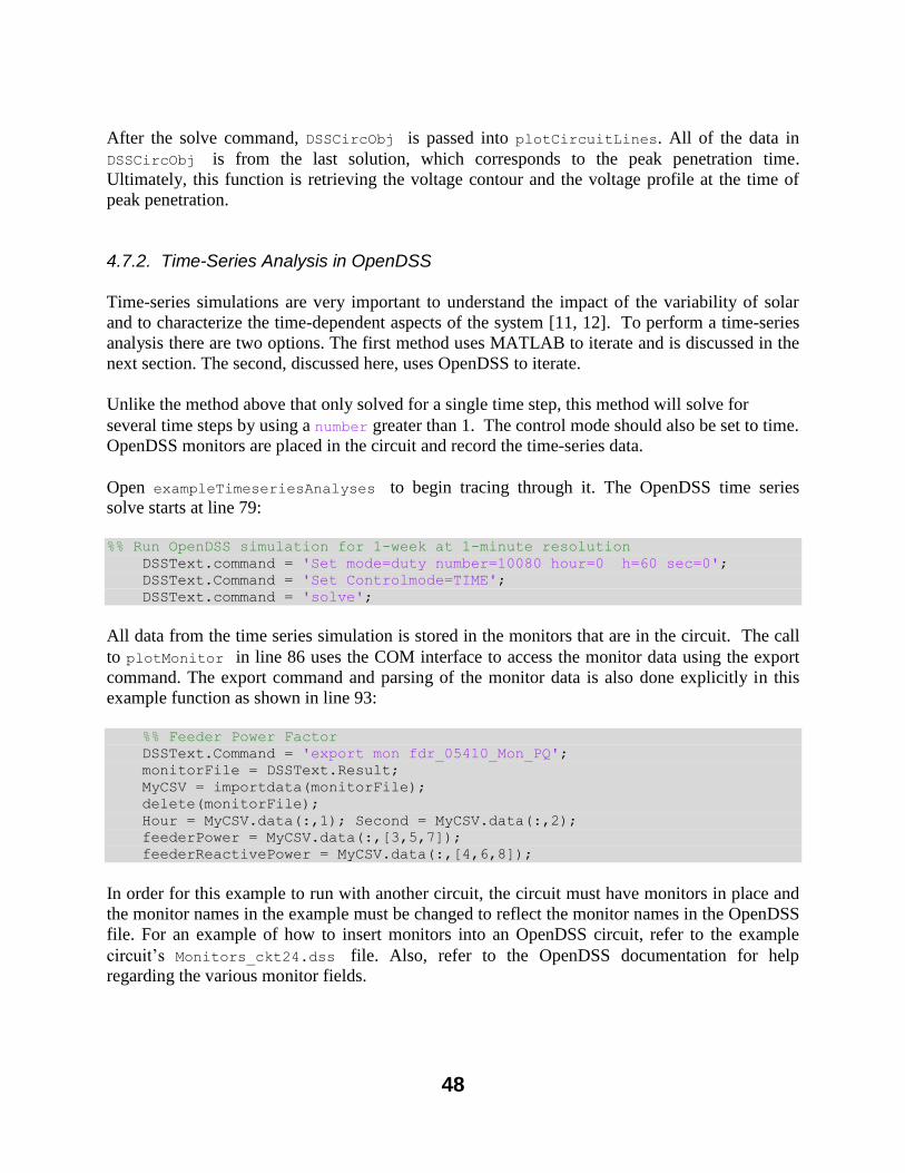
48
After the solve command, DSSCircObj is passed into plotCircuitLines. All of the data in
DSSCircObj is from the last solution, which corresponds to the peak penetration time.
Ultimately, this function is retrieving the voltage contour and the voltage profile at the time of
peak penetration.
4.7.2. Time-Series Analysis in OpenDSS
Time-series simulations are very important to understand the impact of the variability of solar
and to characterize the time-dependent aspects of the system [11, 12]. To perform a time-series
analysis there are two options. The first method uses MATLAB to iterate and is discussed in the
next section. The second, discussed here, uses OpenDSS to iterate.
Unlike the method above that only solved for a single time step, this method will solve for
several time steps by using a number greater than 1. The control mode should also be set to time.
OpenDSS monitors are placed in the circuit and record the time-series data.
Open exampleTimeseriesAnalyses to begin tracing through it. The OpenDSS time series
solve starts at line 79:
%% Run OpenDSS simulation for 1-week at 1-minute resolution DSSText.command = 'Set mode=duty number=10080 hour=0 h=60 sec=0'; DSSText.Command = 'Set Controlmode=TIME'; DSSText.command = 'solve';
All data from the time series simulation is stored in the monitors that are in the circuit. The call
to plotMonitor in line 86 uses the COM interface to access the monitor data using the export
command. The export command and parsing of the monitor data is also done explicitly in this
example function as shown in line 93:
%% Feeder Power Factor DSSText.Command = 'export mon fdr_05410_Mon_PQ'; monitorFile = DSSText.Result; MyCSV = importdata(monitorFile); delete(monitorFile); Hour = MyCSV.data(:,1); Second = MyCSV.data(:,2); feederPower = MyCSV.data(:,[3,5,7]); feederReactivePower = MyCSV.data(:,[4,6,8]);
In order for this example to run with another circuit, the circuit must have monitors in place and
the monitor names in the example must be changed to reflect the monitor names in the OpenDSS
file. For an example of how to insert monitors into an OpenDSS circuit, refer to the example
circuit’s Monitors_ckt24.dss file. Also, refer to the OpenDSS documentation for help
regarding the various monitor fields.
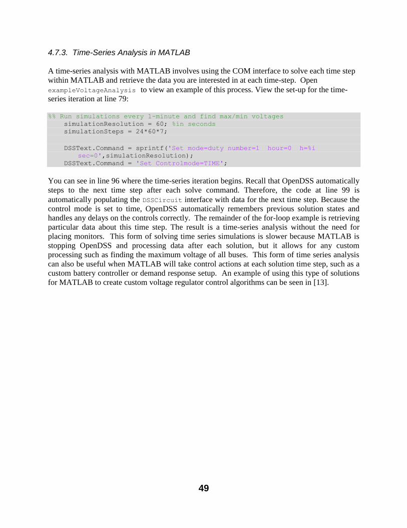
49
4.7.3. Time-Series Analysis in MATLAB
A time-series analysis with MATLAB involves using the COM interface to solve each time step
within MATLAB and retrieve the data you are interested in at each time-step. Open
exampleVoltageAnalysis to view an example of this process. View the set-up for the time-
series iteration at line 79:
%% Run simulations every 1-minute and find max/min voltages simulationResolution = 60; %in seconds simulationSteps = 24*60*7;
DSSText.Command = sprintf('Set mode=duty number=1 hour=0 h=%i
sec=0',simulationResolution); DSSText.Command = 'Set Controlmode=TIME';
You can see in line 96 where the time-series iteration begins. Recall that OpenDSS automatically
steps to the next time step after each solve command. Therefore, the code at line 99 is
automatically populating the DSSCircuit interface with data for the next time step. Because the
control mode is set to time, OpenDSS automatically remembers previous solution states and
handles any delays on the controls correctly. The remainder of the for-loop example is retrieving
particular data about this time step. The result is a time-series analysis without the need for
placing monitors. This form of solving time series simulations is slower because MATLAB is
stopping OpenDSS and processing data after each solution, but it allows for any custom
processing such as finding the maximum voltage of all buses. This form of time series analysis
can also be useful when MATLAB will take control actions at each solution time step, such as a
custom battery controller or demand response setup. An example of using this type of solutions
for MATLAB to create custom voltage regulator control algorithms can be seen in [13].

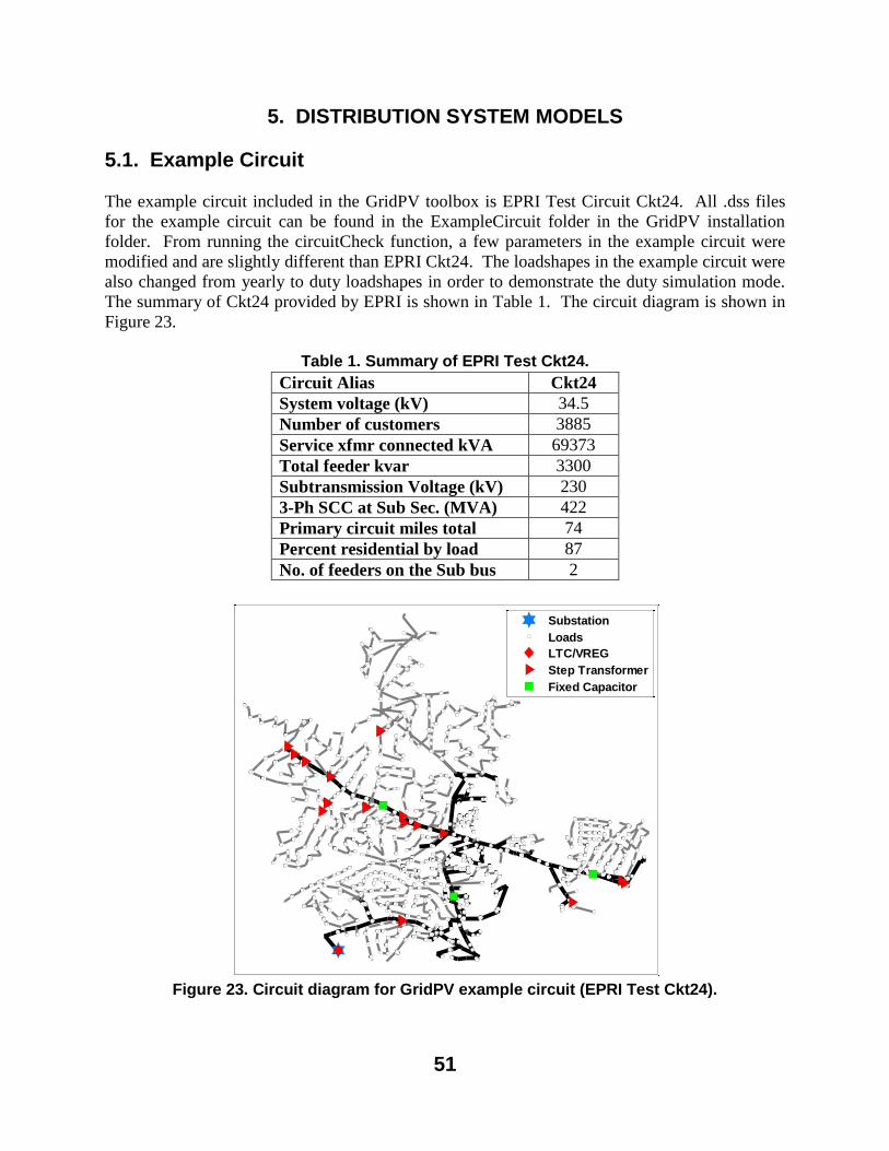
51
5. DISTRIBUTION SYSTEM MODELS
5.1. Example Circuit
The example circuit included in the GridPV toolbox is EPRI Test Circuit Ckt24. All .dss files
for the example circuit can be found in the ExampleCircuit folder in the GridPV installation
folder. From running the circuitCheck function, a few parameters in the example circuit were
modified and are slightly different than EPRI Ckt24. The loadshapes in the example circuit were
also changed from yearly to duty loadshapes in order to demonstrate the duty simulation mode.
The summary of Ckt24 provided by EPRI is shown in Table 1. The circuit diagram is shown in
Figure 23.
Table 1. Summary of EPRI Test Ckt24.
Circuit Alias Ckt24
System voltage (kV) 34.5
Number of customers 3885
Service xfmr connected kVA 69373
Total feeder kvar 3300
Subtransmission Voltage (kV) 230
3-Ph SCC at Sub Sec. (MVA) 422
Primary circuit miles total 74
Percent residential by load 87
No. of feeders on the Sub bus 2
Substation
Loads
LTC/VREG
Step Transformer
Fixed Capacitor
Figure 23. Circuit diagram for GridPV example circuit (EPRI Test Ckt24).
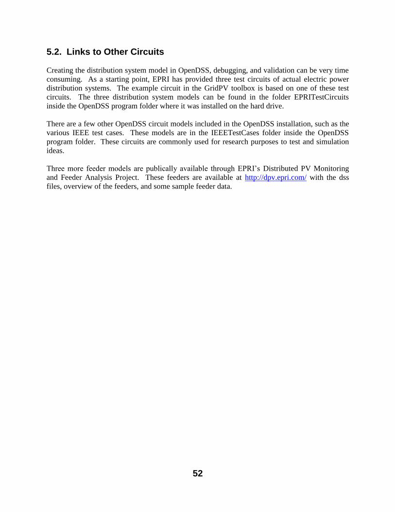
52
5.2. Links to Other Circuits
Creating the distribution system model in OpenDSS, debugging, and validation can be very time
consuming. As a starting point, EPRI has provided three test circuits of actual electric power
distribution systems. The example circuit in the GridPV toolbox is based on one of these test
circuits. The three distribution system models can be found in the folder EPRITestCircuits
inside the OpenDSS program folder where it was installed on the hard drive.
There are a few other OpenDSS circuit models included in the OpenDSS installation, such as the
various IEEE test cases. These models are in the IEEETestCases folder inside the OpenDSS
program folder. These circuits are commonly used for research purposes to test and simulation
ideas.
Three more feeder models are publically available through EPRI’s Distributed PV Monitoring
and Feeder Analysis Project. These feeders are available at http://dpv.epri.com/ with the dss
files, overview of the feeders, and some sample feeder data.
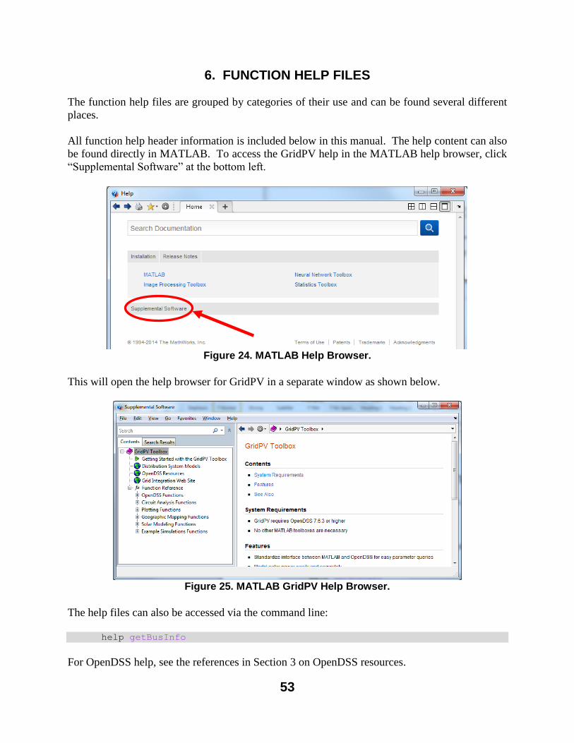
53
6. FUNCTION HELP FILES
The function help files are grouped by categories of their use and can be found several different
places.
All function help header information is included below in this manual. The help content can also
be found directly in MATLAB. To access the GridPV help in the MATLAB help browser, click
“Supplemental Software” at the bottom left.
Figure 24. MATLAB Help Browser.
This will open the help browser for GridPV in a separate window as shown below.
Figure 25. MATLAB GridPV Help Browser.
The help files can also be accessed via the command line:
help getBusInfo
For OpenDSS help, see the references in Section 3 on OpenDSS resources.
54
The functions by category are:
6.1. OpenDSS Functions ............................................................................................................... 55
6.2. Circuit Analysis Functions ..................................................................................................... 84
6.3. Plotting Functions .................................................................................................................. 91
6.4. Geographic Mapping Functions ........................................................................................... 116
6.5. Solar Modeling Functions .................................................................................................... 123
6.6. Example Simulations ........................................................................................................... 139
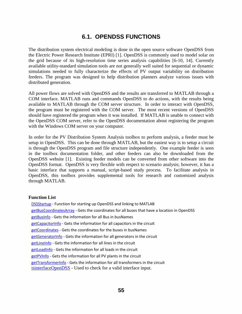
55
6.1. OPENDSS FUNCTIONS
The distribution system electrical modeling is done in the open source software OpenDSS from
the Electric Power Research Institute (EPRI) [1]. OpenDSS is commonly used to model solar on
the grid because of its high-resolution time series analysis capabilities [6-10, 14]. Currently
available utility-standard simulation tools are not generally well suited for sequential or dynamic
simulations needed to fully characterize the effects of PV output variability on distribution
feeders. The program was designed to help distribution planners analyze various issues with
distributed generation.
All power flows are solved with OpenDSS and the results are transferred to MATLAB through a
COM interface. MATLAB runs and commands OpenDSS to do actions, with the results being
available to MATLAB through the COM server structure. In order to interact with OpenDSS,
the program must be registered with the COM server. The most recent versions of OpenDSS
should have registered the program when it was installed. If MATLAB is unable to connect with
the OpenDSS COM server, refer to the OpenDSS documentation about registering the program
with the Windows COM server on your computer.
In order for the PV Distribution System Analysis toolbox to perform analysis, a feeder must be
setup in OpenDSS. This can be done through MATLAB, but the easiest way is to setup a circuit
is through the OpenDSS program and file structure independently. One example feeder is seen
in the toolbox documentation folder, and other feeders can also be downloaded from the
OpenDSS website [1]. Existing feeder models can be converted from other software into the
OpenDSS format. OpenDSS is very flexible with respect to scenario analysis; however, it has a
basic interface that supports a manual, script-based study process. To facilitate analysis in
OpenDSS, this toolbox provides supplemental tools for research and customized analysis
through MATLAB.
Function List
DSSStartup - Function for starting up OpenDSS and linking to MATLAB
getBusCoordinatesArray - Gets the coordinates for all buses that have a location in OpenDSS
getBusInfo - Gets the information for all Bus in busNames
getCapacitorInfo - Gets the information for all capacitors in the circuit
getCoordinates - Gets the coordinates for the buses in busNames
getGeneratorInfo - Gets the information for all generators in the circuit
getLineInfo - Gets the information for all lines in the circuit
getLoadInfo - Gets the information for all loads in the circuit
getPVInfo - Gets the information for all PV plants in the circuit
getTransformerInfo - Gets the information for all transformers in the circuit isinterfaceOpenDSS - Used to check for a valid interface input.
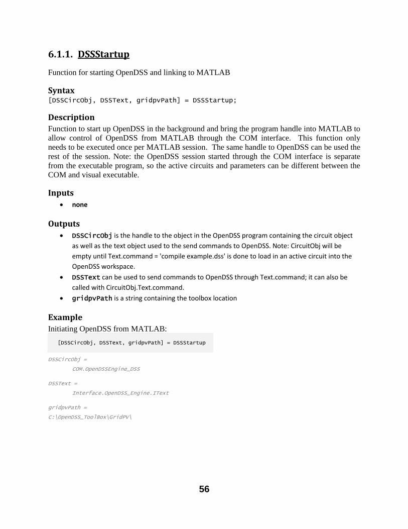
56
6.1.1. DSSStartup
Function for starting OpenDSS and linking to MATLAB
Syntax [DSSCircObj, DSSText, gridpvPath] = DSSStartup;
Description
Function to start up OpenDSS in the background and bring the program handle into MATLAB to
allow control of OpenDSS from MATLAB through the COM interface. This function only
needs to be executed once per MATLAB session. The same handle to OpenDSS can be used the
rest of the session. Note: the OpenDSS session started through the COM interface is separate
from the executable program, so the active circuits and parameters can be different between the
COM and visual executable.
Inputs
none
Outputs
DSSCircObj is the handle to the object in the OpenDSS program containing the circuit object
as well as the text object used to the send commands to OpenDSS. Note: CircuitObj will be
empty until Text.command = 'compile example.dss' is done to load in an active circuit into the
OpenDSS workspace.
DSSText can be used to send commands to OpenDSS through Text.command; it can also be
called with CircuitObj.Text.command.
gridpvPath is a string containing the toolbox location
Example
Initiating OpenDSS from MATLAB:
DSSCircObj = COM.OpenDSSEngine_DSS DSSText = Interface.OpenDSS_Engine.IText gridpvPath = C:\OpenDSS_ToolBox\GridPV\
[DSSCircObj, DSSText, gridpvPath] = DSSStartup
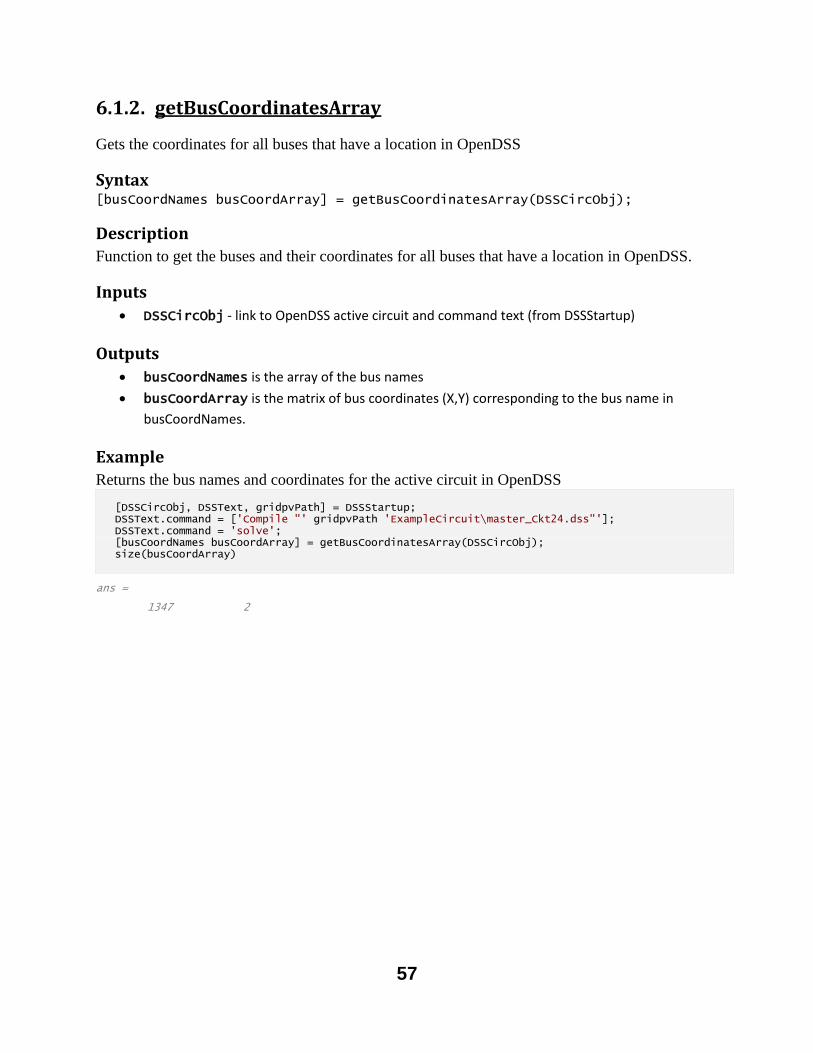
57
6.1.2. getBusCoordinatesArray
Gets the coordinates for all buses that have a location in OpenDSS
Syntax [busCoordNames busCoordArray] = getBusCoordinatesArray(DSSCircObj);
Description
Function to get the buses and their coordinates for all buses that have a location in OpenDSS.
Inputs
DSSCircObj - link to OpenDSS active circuit and command text (from DSSStartup)
Outputs
busCoordNames is the array of the bus names
busCoordArray is the matrix of bus coordinates (X,Y) corresponding to the bus name in
busCoordNames.
Example
Returns the bus names and coordinates for the active circuit in OpenDSS
ans = 1347 2
[DSSCircObj, DSSText, gridpvPath] = DSSStartup; DSSText.command = ['Compile "' gridpvPath 'ExampleCircuit\master_Ckt24.dss"']; DSSText.command = 'solve'; [busCoordNames busCoordArray] = getBusCoordinatesArray(DSSCircObj); size(busCoordArray)
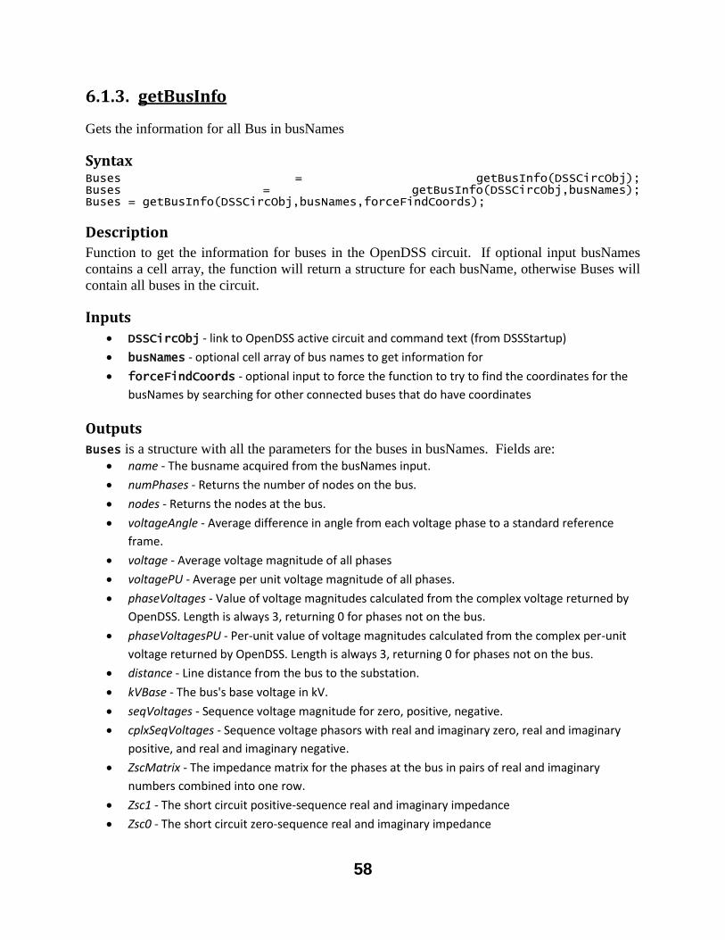
58
6.1.3. getBusInfo
Gets the information for all Bus in busNames
Syntax Buses = getBusInfo(DSSCircObj); Buses = getBusInfo(DSSCircObj,busNames); Buses = getBusInfo(DSSCircObj,busNames,forceFindCoords);
Description
Function to get the information for buses in the OpenDSS circuit. If optional input busNames
contains a cell array, the function will return a structure for each busName, otherwise Buses will
contain all buses in the circuit.
Inputs
DSSCircObj - link to OpenDSS active circuit and command text (from DSSStartup)
busNames - optional cell array of bus names to get information for
forceFindCoords - optional input to force the function to try to find the coordinates for the
busNames by searching for other connected buses that do have coordinates
Outputs
Buses is a structure with all the parameters for the buses in busNames. Fields are:
name - The busname acquired from the busNames input.
numPhases - Returns the number of nodes on the bus.
nodes - Returns the nodes at the bus.
voltageAngle - Average difference in angle from each voltage phase to a standard reference
frame.
voltage - Average voltage magnitude of all phases
voltagePU - Average per unit voltage magnitude of all phases.
phaseVoltages - Value of voltage magnitudes calculated from the complex voltage returned by
OpenDSS. Length is always 3, returning 0 for phases not on the bus.
phaseVoltagesPU - Per-unit value of voltage magnitudes calculated from the complex per-unit
voltage returned by OpenDSS. Length is always 3, returning 0 for phases not on the bus.
distance - Line distance from the bus to the substation.
kVBase - The bus's base voltage in kV.
seqVoltages - Sequence voltage magnitude for zero, positive, negative.
cplxSeqVoltages - Sequence voltage phasors with real and imaginary zero, real and imaginary
positive, and real and imaginary negative.
ZscMatrix - The impedance matrix for the phases at the bus in pairs of real and imaginary
numbers combined into one row.
Zsc1 - The short circuit positive-sequence real and imaginary impedance
Zsc0 - The short circuit zero-sequence real and imaginary impedance

59
YscMatrix - The admittance matrix for the phases at the bus in pairs of real and imaginary
numbers combined into one row.
coordinates - Returns coordinates stored in OpenDSS for the active bus. If coordinates do not
exist and forceFindCoords is 1, it returns coordinates of the coordinates of the nearest upstream
element.
Example
Returns bus information
Buses = 6058x1 struct array with fields: name numPhases nodes voltageAngle voltage voltagePU phaseVoltages phaseVoltagesPU distance kVBase seqVoltages cplxSeqVoltages ZscMatrix Zsc1 Zsc0 YscMatrix coordinates Buses = name: 'N1311915' numPhases: 1 nodes: 1 voltageAngle: 0.6600 voltage: 2.0362e+04 voltagePU: 1.0223 phaseVoltages: [2.0362e+04 0 0] phaseVoltagesPU: [1.0223 0 0] distance: 2.3813 kVBase: 19.9186 seqVoltages: [-1 -1 -1] cplxSeqVoltages: [-1 -1 -1 -1 -1 -1] ZscMatrix: 0 Zsc1: [0 0] Zsc0: [0 0] YscMatrix: 0 coordinates: [31.6145 -80.9461]
[DSSCircObj, DSSText, gridpvPath] = DSSStartup; DSSText.command = ['Compile "' gridpvPath 'ExampleCircuit\master_Ckt24.dss"']; DSSText.command = 'solve'; Buses = getBusInfo(DSSCircObj) %Get information for all buses Buses = getBusInfo(DSSCircObj,{'N1311915'}) %Get information for one bus
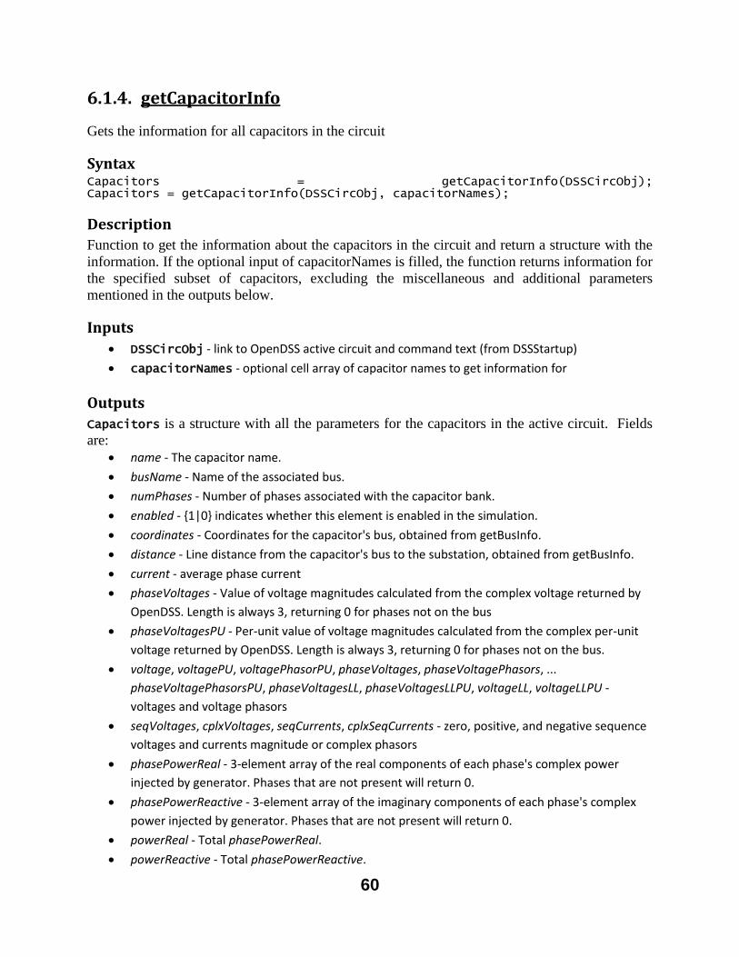
60
6.1.4. getCapacitorInfo
Gets the information for all capacitors in the circuit
Syntax Capacitors = getCapacitorInfo(DSSCircObj); Capacitors = getCapacitorInfo(DSSCircObj, capacitorNames);
Description
Function to get the information about the capacitors in the circuit and return a structure with the
information. If the optional input of capacitorNames is filled, the function returns information for
the specified subset of capacitors, excluding the miscellaneous and additional parameters
mentioned in the outputs below.
Inputs
DSSCircObj - link to OpenDSS active circuit and command text (from DSSStartup)
capacitorNames - optional cell array of capacitor names to get information for
Outputs
Capacitors is a structure with all the parameters for the capacitors in the active circuit. Fields
are:
name - The capacitor name.
busName - Name of the associated bus.
numPhases - Number of phases associated with the capacitor bank.
enabled - {1|0} indicates whether this element is enabled in the simulation.
coordinates - Coordinates for the capacitor's bus, obtained from getBusInfo.
distance - Line distance from the capacitor's bus to the substation, obtained from getBusInfo.
current - average phase current
phaseVoltages - Value of voltage magnitudes calculated from the complex voltage returned by
OpenDSS. Length is always 3, returning 0 for phases not on the bus
phaseVoltagesPU - Per-unit value of voltage magnitudes calculated from the complex per-unit
voltage returned by OpenDSS. Length is always 3, returning 0 for phases not on the bus.
voltage, voltagePU, voltagePhasorPU, phaseVoltages, phaseVoltagePhasors, ...
phaseVoltagePhasorsPU, phaseVoltagesLL, phaseVoltagesLLPU, voltageLL, voltageLLPU -
voltages and voltage phasors
seqVoltages, cplxVoltages, seqCurrents, cplxSeqCurrents - zero, positive, and negative sequence
voltages and currents magnitude or complex phasors
phasePowerReal - 3-element array of the real components of each phase's complex power
injected by generator. Phases that are not present will return 0.
phasePowerReactive - 3-element array of the imaginary components of each phase's complex
power injected by generator. Phases that are not present will return 0.
powerReal - Total phasePowerReal.
powerReactive - Total phasePowerReactive.
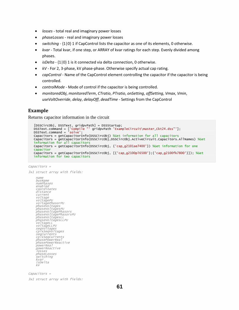
61
losses - total real and imaginary power losses
phaseLosses - real and imaginary power losses
switching - {1|0} 1 if CapControl lists the capacitor as one of its elements, 0 otherwise.
kvar - Total kvar, if one step, or ARRAY of kvar ratings for each step. Evenly divided among
phases.
isDelta - {1|0} 1 is it connected via delta connection, 0 otherwise.
kV - For 2, 3-phase, kV phase-phase. Otherwise specify actual cap rating.
capControl - Name of the CapControl element controlling the capacitor if the capacitor is being
controlled.
controlMode - Mode of control if the capacitor is being controlled.
monitoredObj, monitoredTerm, CTratio, PTratio, onSetting, offSetting, Vmax, Vmin,
useVoltOverride, delay, delayOff, deadTime - Settings from the CapControl
Example
Returns capacitor information in the circuit
Capacitors = 3x1 struct array with fields: name busName numPhases enabled coordinates distance current voltage voltagePU voltagePhasorPU phaseVoltages phaseVoltagesPU phaseVoltagePhasors phaseVoltagePhasorsPU phaseVoltagesLL phaseVoltagesLLPU voltageLL voltageLLPU seqVoltages cplxSeqVoltages seqCurrents cplxSeqCurrents phasePowerReal phasePowerReactive powerReal powerReactive losses phaseLosses switching kvar isDelta kV Capacitors = 3x1 struct array with fields:
[DSSCircObj, DSSText, gridpvPath] = DSSStartup; DSSText.command = ['Compile "' gridpvPath 'ExampleCircuit\master_Ckt24.dss"']; DSSText.command = 'solve'; Capacitors = getCapacitorInfo(DSSCircObj) %Get information for all capacitors Capacitors = getCapacitorInfo(DSSCircObj,DSSCircObj.ActiveCircuit.Capacitors.AllNames) %Get information for all capacitors Capacitors = getCapacitorInfo(DSSCircObj, {'cap_g2101ae7400'}) %Get information for one capacitor Capacitors = getCapacitorInfo(DSSCircObj, [{'cap_g2100pl6500'};{'cap_g2100fk7800'}]); %Get information for two capacitors
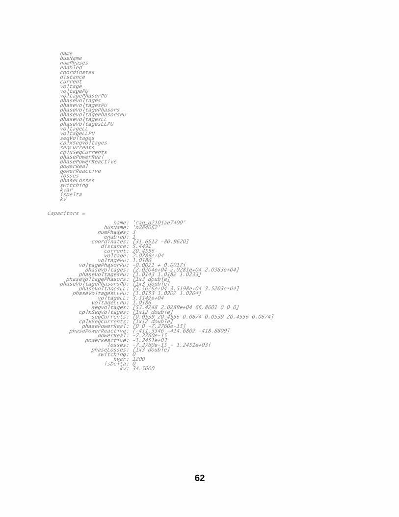
62
name busName numPhases enabled coordinates distance current voltage voltagePU voltagePhasorPU phaseVoltages phaseVoltagesPU phaseVoltagePhasors phaseVoltagePhasorsPU phaseVoltagesLL phaseVoltagesLLPU voltageLL voltageLLPU seqVoltages cplxSeqVoltages seqCurrents cplxSeqCurrents phasePowerReal phasePowerReactive powerReal powerReactive losses phaseLosses switching kvar isDelta kV Capacitors = name: 'cap_g2101ae7400' busName: 'n284062' numPhases: 3 enabled: 1 coordinates: [31.6512 -80.9620] distance: 5.4491 current: 20.4556 voltage: 2.0289e+04 voltagePU: 1.0186 voltagePhasorPU: -0.0021 + 0.0017i phaseVoltages: [2.0204e+04 2.0281e+04 2.0383e+04] phaseVoltagesPU: [1.0143 1.0182 1.0233] phaseVoltagePhasors: [1x3 double] phaseVoltagePhasorsPU: [1x3 double] phaseVoltagesLL: [3.5026e+04 3.5198e+04 3.5203e+04] phaseVoltagesLLPU: [1.0153 1.0202 1.0204] voltageLL: 3.5142e+04 voltageLLPU: 1.0186 seqVoltages: [53.4248 2.0289e+04 66.8601 0 0 0] cplxSeqVoltages: [1x12 double] seqCurrents: [0.0539 20.4556 0.0674 0.0539 20.4556 0.0674] cplxSeqCurrents: [1x12 double] phasePowerReal: [0 0 -7.2760e-15] phasePowerReactive: [-411.5546 -414.6802 -418.8809] powerReal: -7.2760e-15 powerReactive: -1.2451e+03 losses: -7.2760e-15 - 1.2451e+03i phaseLosses: [1x3 double] switching: 0 kvar: 1200 isDelta: 0 kV: 34.5000
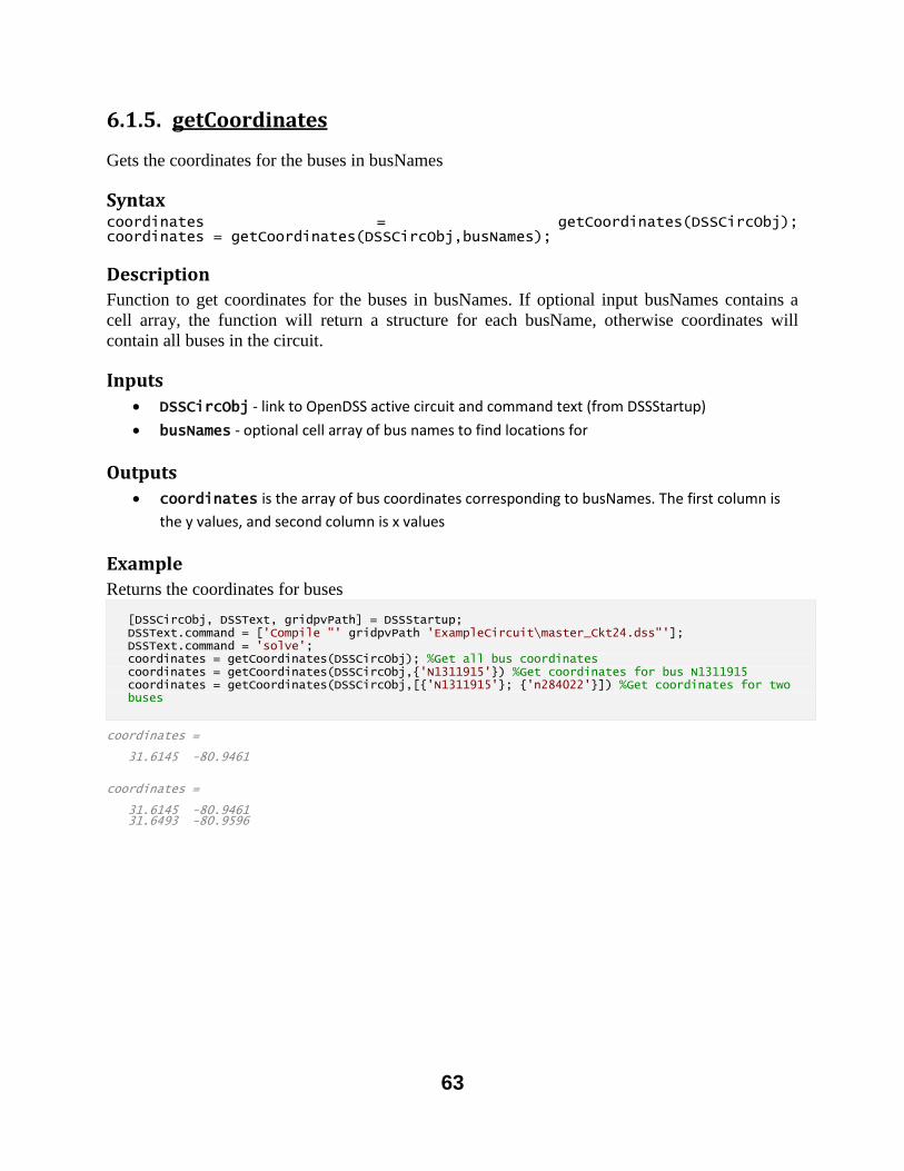
63
6.1.5. getCoordinates
Gets the coordinates for the buses in busNames
Syntax coordinates = getCoordinates(DSSCircObj); coordinates = getCoordinates(DSSCircObj,busNames);
Description
Function to get coordinates for the buses in busNames. If optional input busNames contains a
cell array, the function will return a structure for each busName, otherwise coordinates will
contain all buses in the circuit.
Inputs
DSSCircObj - link to OpenDSS active circuit and command text (from DSSStartup)
busNames - optional cell array of bus names to find locations for
Outputs
coordinates is the array of bus coordinates corresponding to busNames. The first column is
the y values, and second column is x values
Example
Returns the coordinates for buses
coordinates = 31.6145 -80.9461 coordinates = 31.6145 -80.9461 31.6493 -80.9596
[DSSCircObj, DSSText, gridpvPath] = DSSStartup; DSSText.command = ['Compile "' gridpvPath 'ExampleCircuit\master_Ckt24.dss"']; DSSText.command = 'solve'; coordinates = getCoordinates(DSSCircObj); %Get all bus coordinates coordinates = getCoordinates(DSSCircObj,{'N1311915'}) %Get coordinates for bus N1311915 coordinates = getCoordinates(DSSCircObj,[{'N1311915'}; {'n284022'}]) %Get coordinates for two buses

64
6.1.6. getGeneratorInfo
Gets the information for all generators in the circuit
Syntax Generators = getGeneratorInfo(DSSCircObj); Generators = getGeneratorInfo(DSSCircObj, generatorNames);
Description
Function to get the information about the generators in the circuit and return a structure with the
information. If the optional input of generatorNames is filled, the function returns information
for the specified subset of generators, excluding the miscellaneous parameters mentioned in the
outputs below.
Inputs
DSSCircObj - link to OpenDSS active circuit and command text (from DSSStartup)
generatorNames - optional cell array of generator names to get information for
Outputs
Generators is a structure with all the parameters for the generators in the active circuit. Fields
are:
name - Name of the generator.
busName - Name of the associated bus.
numPhases - Number of phases associated with the generator.
enabled - {1|0} indicates whether this element is enabled in the simulation.
nodes - the connection nodes at the bus
current - average phase current output
coordinates - Coordinates for the bus
distance - Line distance from the bus to the substation
phaseVoltages - Value of voltage magnitudes calculated from the complex voltage returned by
OpenDSS. Length is always 3, returning 0 for phases not on the bus
phaseVoltagesPU - Per-unit value of voltage magnitudes calculated from the complex per-unit
voltage returned by OpenDSS. Length is always 3, returning 0 for phases not on the bus.
voltage, voltagePU, voltagePhasorPU, phaseVoltages, phaseVoltagePhasors, ...
phaseVoltagePhasorsPU, phaseVoltagesLL, phaseVoltagesLLPU, voltageLL, voltageLLPU -
voltages and voltage phasors
phasePowerReal - 3-element array of the real components of each phase's complex power
injected by generator. Phases that are not present will return 0.
phasePowerReactive - 3-element array of the imaginary components of each phase's complex
power injected by generator. Phases that are not present will return 0.
powerReal - Total phasePowerReal.
powerReactive - Total phasePowerReactive.
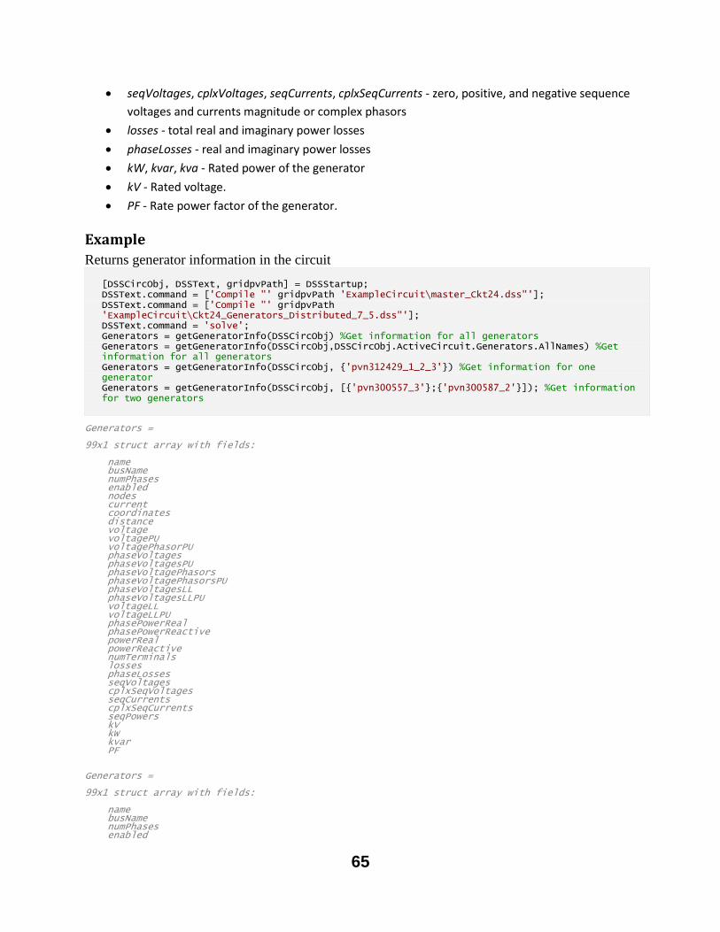
65
seqVoltages, cplxVoltages, seqCurrents, cplxSeqCurrents - zero, positive, and negative sequence
voltages and currents magnitude or complex phasors
losses - total real and imaginary power losses
phaseLosses - real and imaginary power losses
kW, kvar, kva - Rated power of the generator
kV - Rated voltage.
PF - Rate power factor of the generator.
Example
Returns generator information in the circuit
Generators = 99x1 struct array with fields: name busName numPhases enabled nodes current coordinates distance voltage voltagePU voltagePhasorPU phaseVoltages phaseVoltagesPU phaseVoltagePhasors phaseVoltagePhasorsPU phaseVoltagesLL phaseVoltagesLLPU voltageLL voltageLLPU phasePowerReal phasePowerReactive powerReal powerReactive numTerminals losses phaseLosses seqVoltages cplxSeqVoltages seqCurrents cplxSeqCurrents seqPowers kV kW kvar PF Generators = 99x1 struct array with fields: name busName numPhases enabled
[DSSCircObj, DSSText, gridpvPath] = DSSStartup; DSSText.command = ['Compile "' gridpvPath 'ExampleCircuit\master_Ckt24.dss"']; DSSText.command = ['Compile "' gridpvPath 'ExampleCircuit\Ckt24_Generators_Distributed_7_5.dss"']; DSSText.command = 'solve'; Generators = getGeneratorInfo(DSSCircObj) %Get information for all generators Generators = getGeneratorInfo(DSSCircObj,DSSCircObj.ActiveCircuit.Generators.AllNames) %Get information for all generators Generators = getGeneratorInfo(DSSCircObj, {'pvn312429_1_2_3'}) %Get information for one generator Generators = getGeneratorInfo(DSSCircObj, [{'pvn300557_3'};{'pvn300587_2'}]); %Get information for two generators
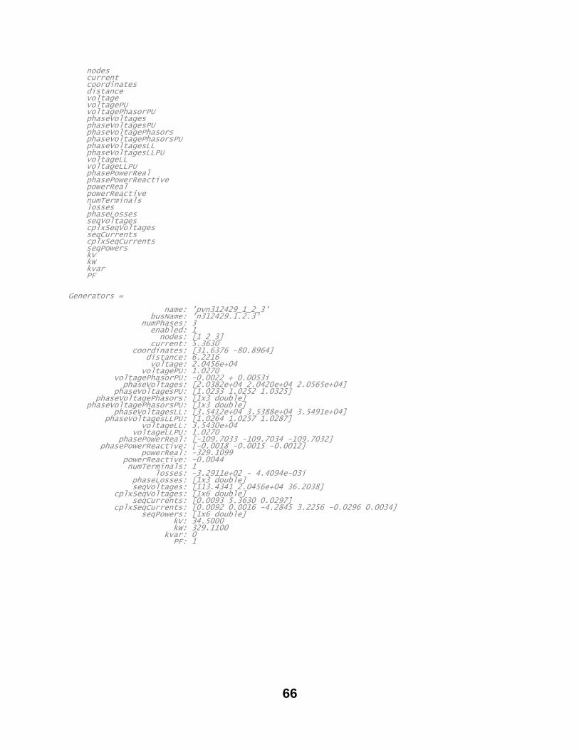
66
nodes current coordinates distance voltage voltagePU voltagePhasorPU phaseVoltages phaseVoltagesPU phaseVoltagePhasors phaseVoltagePhasorsPU phaseVoltagesLL phaseVoltagesLLPU voltageLL voltageLLPU phasePowerReal phasePowerReactive powerReal powerReactive numTerminals losses phaseLosses seqVoltages cplxSeqVoltages seqCurrents cplxSeqCurrents seqPowers kV kW kvar PF Generators = name: 'pvn312429_1_2_3' busName: 'n312429.1.2.3' numPhases: 3 enabled: 1 nodes: [1 2 3] current: 5.3630 coordinates: [31.6376 -80.8964] distance: 6.2216 voltage: 2.0456e+04 voltagePU: 1.0270 voltagePhasorPU: -0.0022 + 0.0053i phaseVoltages: [2.0382e+04 2.0420e+04 2.0565e+04] phaseVoltagesPU: [1.0233 1.0252 1.0325] phaseVoltagePhasors: [1x3 double] phaseVoltagePhasorsPU: [1x3 double] phaseVoltagesLL: [3.5412e+04 3.5388e+04 3.5491e+04] phaseVoltagesLLPU: [1.0264 1.0257 1.0287] voltageLL: 3.5430e+04 voltageLLPU: 1.0270 phasePowerReal: [-109.7033 -109.7034 -109.7032] phasePowerReactive: [-0.0018 -0.0015 -0.0012] powerReal: -329.1099 powerReactive: -0.0044 numTerminals: 1 losses: -3.2911e+02 - 4.4094e-03i phaseLosses: [1x3 double] seqVoltages: [113.4341 2.0456e+04 36.2038] cplxSeqVoltages: [1x6 double] seqCurrents: [0.0093 5.3630 0.0297] cplxSeqCurrents: [0.0092 0.0016 -4.2845 3.2256 -0.0296 0.0034] seqPowers: [1x6 double] kV: 34.5000 kW: 329.1100 kvar: 0 PF: 1
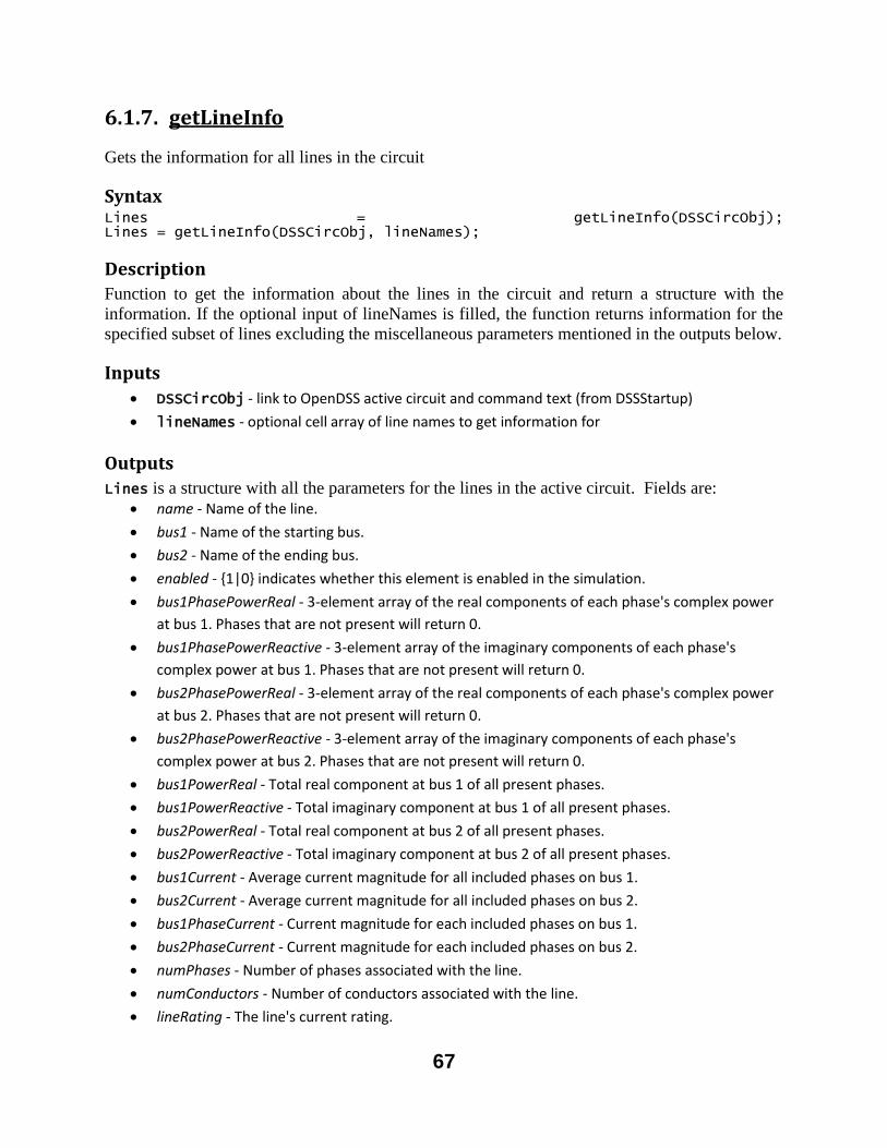
67
6.1.7. getLineInfo
Gets the information for all lines in the circuit
Syntax Lines = getLineInfo(DSSCircObj); Lines = getLineInfo(DSSCircObj, lineNames);
Description
Function to get the information about the lines in the circuit and return a structure with the
information. If the optional input of lineNames is filled, the function returns information for the
specified subset of lines excluding the miscellaneous parameters mentioned in the outputs below.
Inputs
DSSCircObj - link to OpenDSS active circuit and command text (from DSSStartup)
lineNames - optional cell array of line names to get information for
Outputs
Lines is a structure with all the parameters for the lines in the active circuit. Fields are:
name - Name of the line.
bus1 - Name of the starting bus.
bus2 - Name of the ending bus.
enabled - {1|0} indicates whether this element is enabled in the simulation.
bus1PhasePowerReal - 3-element array of the real components of each phase's complex power
at bus 1. Phases that are not present will return 0.
bus1PhasePowerReactive - 3-element array of the imaginary components of each phase's
complex power at bus 1. Phases that are not present will return 0.
bus2PhasePowerReal - 3-element array of the real components of each phase's complex power
at bus 2. Phases that are not present will return 0.
bus2PhasePowerReactive - 3-element array of the imaginary components of each phase's
complex power at bus 2. Phases that are not present will return 0.
bus1PowerReal - Total real component at bus 1 of all present phases.
bus1PowerReactive - Total imaginary component at bus 1 of all present phases.
bus2PowerReal - Total real component at bus 2 of all present phases.
bus2PowerReactive - Total imaginary component at bus 2 of all present phases.
bus1Current - Average current magnitude for all included phases on bus 1.
bus2Current - Average current magnitude for all included phases on bus 2.
bus1PhaseCurrent - Current magnitude for each included phases on bus 1.
bus2PhaseCurrent - Current magnitude for each included phases on bus 2.
numPhases - Number of phases associated with the line.
numConductors - Number of conductors associated with the line.
lineRating - The line's current rating.
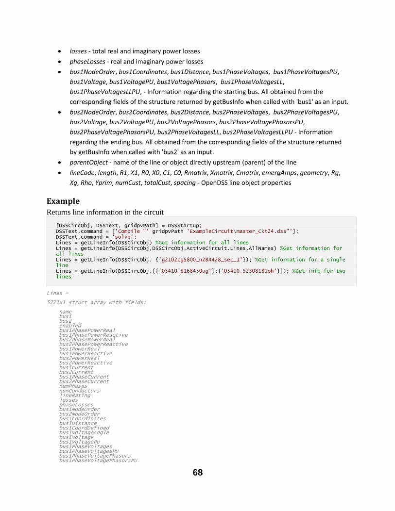
68
losses - total real and imaginary power losses
phaseLosses - real and imaginary power losses
bus1NodeOrder, bus1Coordinates, bus1Distance, bus1PhaseVoltages, bus1PhaseVoltagesPU,
bus1Voltage, bus1VoltagePU, bus1VoltagePhasors, bus1PhaseVoltagesLL,
bus1PhaseVoltagesLLPU, - Information regarding the starting bus. All obtained from the
corresponding fields of the structure returned by getBusInfo when called with 'bus1' as an input.
bus2NodeOrder, bus2Coordinates, bus2Distance, bus2PhaseVoltages, bus2PhaseVoltagesPU,
bus2Voltage, bus2VoltagePU, bus2VoltagePhasors, bus2PhaseVoltagePhasorsPU,
bus2PhaseVoltagePhasorsPU, bus2PhaseVoltagesLL, bus2PhaseVoltagesLLPU - Information
regarding the ending bus. All obtained from the corresponding fields of the structure returned
by getBusInfo when called with 'bus2' as an input.
parentObject - name of the line or object directly upstream (parent) of the line
lineCode, length, R1, X1, R0, X0, C1, C0, Rmatrix, Xmatrix, Cmatrix, emergAmps, geometry, Rg,
Xg, Rho, Yprim, numCust, totalCust, spacing - OpenDSS line object properties
Example
Returns line information in the circuit
Lines = 5221x1 struct array with fields: name bus1 bus2 enabled bus1PhasePowerReal bus1PhasePowerReactive bus2PhasePowerReal bus2PhasePowerReactive bus1PowerReal bus1PowerReactive bus2PowerReal bus2PowerReactive bus1Current bus2Current bus1PhaseCurrent bus2PhaseCurrent numPhases numConductors lineRating losses phaseLosses bus1NodeOrder bus2NodeOrder bus1Coordinates bus1Distance bus1CoordDefined bus1VoltageAngle bus1Voltage bus1VoltagePU bus1PhaseVoltages bus1PhaseVoltagesPU bus1PhaseVoltagePhasors bus1PhaseVoltagePhasorsPU
[DSSCircObj, DSSText, gridpvPath] = DSSStartup; DSSText.command = ['Compile "' gridpvPath 'ExampleCircuit\master_Ckt24.dss"']; DSSText.command = 'solve'; Lines = getLineInfo(DSSCircObj) %Get information for all lines Lines = getLineInfo(DSSCircObj,DSSCircObj.ActiveCircuit.Lines.AllNames) %Get information for all lines Lines = getLineInfo(DSSCircObj, {'g2102cg5800_n284428_sec_1'}); %Get information for a single line Lines = getLineInfo(DSSCircObj,[{'05410_8168450ug'};{'05410_52308181oh'}]); %Get info for two lines
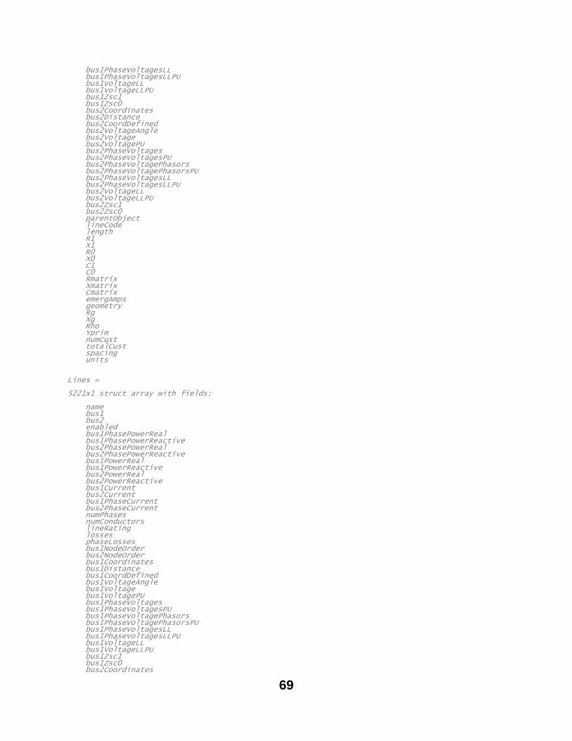
69
bus1PhaseVoltagesLL bus1PhaseVoltagesLLPU bus1VoltageLL bus1VoltageLLPU bus1Zsc1 bus1Zsc0 bus2Coordinates bus2Distance bus2CoordDefined bus2VoltageAngle bus2Voltage bus2VoltagePU bus2PhaseVoltages bus2PhaseVoltagesPU bus2PhaseVoltagePhasors bus2PhaseVoltagePhasorsPU bus2PhaseVoltagesLL bus2PhaseVoltagesLLPU bus2VoltageLL bus2VoltageLLPU bus2Zsc1 bus2Zsc0 parentObject lineCode length R1 X1 R0 X0 C1 C0 Rmatrix Xmatrix Cmatrix emergAmps geometry Rg Xg Rho Yprim numCust totalCust spacing units Lines = 5221x1 struct array with fields: name bus1 bus2 enabled bus1PhasePowerReal bus1PhasePowerReactive bus2PhasePowerReal bus2PhasePowerReactive bus1PowerReal bus1PowerReactive bus2PowerReal bus2PowerReactive bus1Current bus2Current bus1PhaseCurrent bus2PhaseCurrent numPhases numConductors lineRating losses phaseLosses bus1NodeOrder bus2NodeOrder bus1Coordinates bus1Distance bus1CoordDefined bus1VoltageAngle bus1Voltage bus1VoltagePU bus1PhaseVoltages bus1PhaseVoltagesPU bus1PhaseVoltagePhasors bus1PhaseVoltagePhasorsPU bus1PhaseVoltagesLL bus1PhaseVoltagesLLPU bus1VoltageLL bus1VoltageLLPU bus1Zsc1 bus1Zsc0 bus2Coordinates
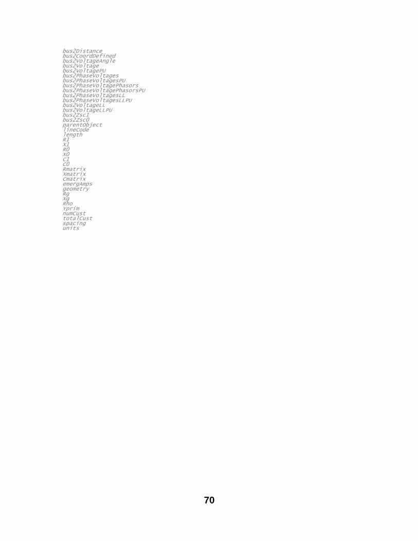
70
bus2Distance bus2CoordDefined bus2VoltageAngle bus2Voltage bus2VoltagePU bus2PhaseVoltages bus2PhaseVoltagesPU bus2PhaseVoltagePhasors bus2PhaseVoltagePhasorsPU bus2PhaseVoltagesLL bus2PhaseVoltagesLLPU bus2VoltageLL bus2VoltageLLPU bus2Zsc1 bus2Zsc0 parentObject lineCode length R1 X1 R0 X0 C1 C0 Rmatrix Xmatrix Cmatrix emergAmps geometry Rg Xg Rho Yprim numCust totalCust spacing units

71
6.1.8. getLoadInfo
Gets the information for all loads in the circuit
Syntax Loads = getLoadInfo(DSSCircObj) Loads = getLoadInfo(DSSCircObj, loadNames)
Description
Function to get the information about the loads in the circuit and return a structure with the
information. If the optional input of loadNames is filled, the function returns information for the
specified subset of loads, excluding the miscellaneous parameters mentioned in the outputs
below.
Inputs
DSSCircObj - link to OpenDSS active circuit and command text (from DSSStartup)
loadNames - optional cell array of line names to get information for
Outputs
Loads is a structure with all the parameters for the loads in the active circuit. Fields are:
name - Name of the load.
busName - Name of the associated bus.
numPhases - Number of phases associated with the load.
enabled - {1|0} indicates whether this element is enabled in the simulation.
coordinates - Coordinates for the load's bus, obtained from getBusInfo.
distance - Line distance from the load's bus to the substation, obtained from getBusInfo.
current - average phase current
phaseVoltages - Value of voltage magnitudes calculated from the complex voltage returned by
OpenDSS. Length is always 3, returning 0 for phases not on the bus
phaseVoltagesPU - Per-unit value of voltage magnitudes calculated from the complex per-unit
voltage returned by OpenDSS. Length is always 3, returning 0 for phases not on the bus.
voltage, voltagePU, voltagePhasorPU, phaseVoltages, phaseVoltagePhasors, ...
phaseVoltagePhasorsPU, phaseVoltagesLL, phaseVoltagesLLPU, voltageLL, voltageLLPU -
voltages and voltage phasors
seqVoltages, cplxVoltages, seqCurrents, cplxSeqCurrents - zero, positive, and negative sequence
voltages and currents magnitude or complex phasors
phasePowerReal - 3-element array of the real components of each phase's complex power
injected by generator. Phases that are not present will return 0.
phasePowerReactive - 3-element array of the imaginary components of each phase's complex
power injected by generator. Phases that are not present will return 0.
powerReal - Total phasePowerReal.
powerReactive - Total phasePowerReactive.
losses - total real and imaginary power losses
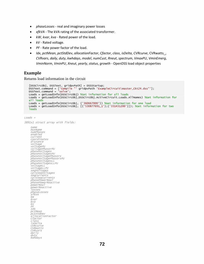
72
phaseLosses - real and imaginary power losses
xfkVA - The kVA rating of the associated transformer.
kW, kvar, kva - Rated power of the load.
kV - Rated voltage.
PF - Rate power factor of the load.
Idx, pctMean, pctStdDev, allocationFactor, Cfactor, class, isDelta, CVRcurve, CVRwatts_,
CVRvars, daily, duty, kwhdays, model, numCust, Rneut, spectrum, VmaxPU, VminEmerg,
VminNorm, VminPU, Xneut, yearly, status, growth - OpenDSS load object properties
Example
Returns load information in the circuit
Loads = 3891x1 struct array with fields: name busName numPhases enabled current coordinates distance voltage voltagePU voltagePhasorPU phaseVoltages phaseVoltagesPU phaseVoltagePhasors phaseVoltagePhasorsPU phaseVoltagesLL phaseVoltagesLLPU voltageLL voltageLLPU seqVoltages cplxSeqVoltages seqCurrents cplxSeqCurrents phasePowerReal phasePowerReactive powerReal powerReactive losses phaseLosses xfkVA kW kvar kva kV PF Idx pctMean pctStdDev allocationFactor Cfactor class isDelta CVRcurve CVRwatts CVRvars daily duty kwhdays
[DSSCircObj, DSSText, gridpvPath] = DSSStartup; DSSText.command = ['Compile "' gridpvPath 'ExampleCircuit\master_Ckt24.dss"']; DSSText.command = 'solve'; Loads = getLoadInfo(DSSCircObj) %Get information for all loads Loads = getLoadInfo(DSSCircObj,DSSCircObj.ActiveCircuit.Loads.AllNames) %Get information for all loads Loads = getLoadInfo(DSSCircObj, {'360667000'}) %Get information for one load Loads = getLoadInfo(DSSCircObj, [{'530877691_1'};{'331431200'}]); %Get information for two loads
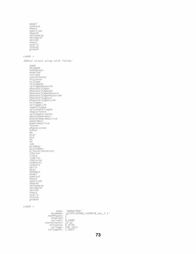
73
model numCust Rneut spectrum VmaxPU VminEmerg VminNorm VminPU Xneut yearly status growth Loads = 3891x1 struct array with fields: name busName numPhases enabled current coordinates distance voltage voltagePU voltagePhasorPU phaseVoltages phaseVoltagesPU phaseVoltagePhasors phaseVoltagePhasorsPU phaseVoltagesLL phaseVoltagesLLPU voltageLL voltageLLPU seqVoltages cplxSeqVoltages seqCurrents cplxSeqCurrents phasePowerReal phasePowerReactive powerReal powerReactive losses phaseLosses xfkVA kW kvar kva kV PF Idx pctMean pctStdDev allocationFactor Cfactor class isDelta CVRcurve CVRwatts CVRvars daily duty kwhdays model numCust Rneut spectrum VmaxPU VminEmerg VminNorm VminPU Xneut yearly status growth Loads = name: '360667000' busName: 'g2101ra0900_n300678_sec_2.1' numPhases: 1 enabled: 1 current: 0.0489 coordinates: [0 0] distance: 6.9739 voltage: 240.1923 voltagePU: 1.0025
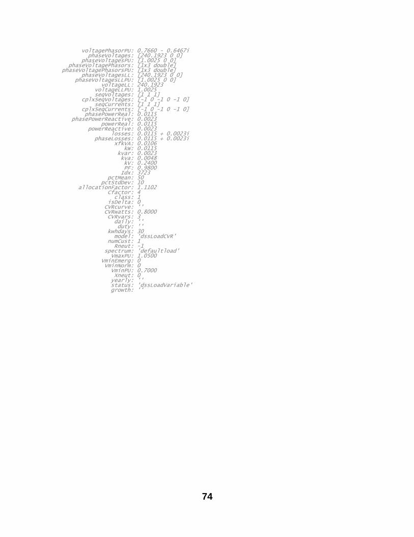
74
voltagePhasorPU: 0.7660 - 0.6467i phaseVoltages: [240.1923 0 0] phaseVoltagesPU: [1.0025 0 0] phaseVoltagePhasors: [1x3 double] phaseVoltagePhasorsPU: [1x3 double] phaseVoltagesLL: [240.1923 0 0] phaseVoltagesLLPU: [1.0025 0 0] voltageLL: 240.1923 voltageLLPU: 1.0025 seqVoltages: [1 1 1] cplxSeqVoltages: [-1 0 -1 0 -1 0] seqCurrents: [1 1 1] cplxSeqCurrents: [-1 0 -1 0 -1 0] phasePowerReal: 0.0115 phasePowerReactive: 0.0023 powerReal: 0.0115 powerReactive: 0.0023 losses: 0.0115 + 0.0023i phaseLosses: 0.0115 + 0.0023i xfkVA: 0.0106 kW: 0.0115 kvar: 0.0023 kva: 0.0048 kV: 0.2400 PF: 0.9800 Idx: 3723 pctMean: 50 pctStdDev: 10 allocationFactor: 1.1102 Cfactor: 4 class: 1 isDelta: 0 CVRcurve: '' CVRwatts: 0.8000 CVRvars: 3 daily: '' duty: '' kwhdays: 30 model: 'dssLoadCVR' numCust: 1 Rneut: -1 spectrum: 'defaultload' VmaxPU: 1.0500 VminEmerg: 0 VminNorm: 0 VminPU: 0.7000 Xneut: 0 yearly: '' status: 'dssLoadVariable' growth: ''
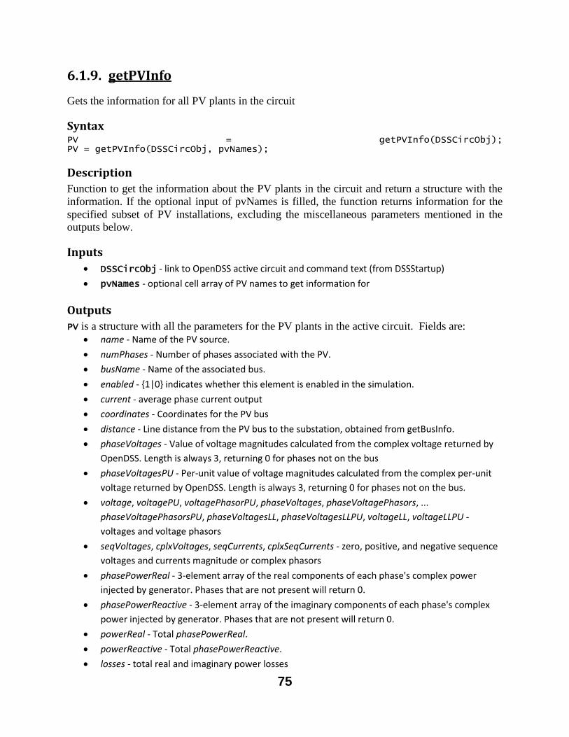
75
6.1.9. getPVInfo
Gets the information for all PV plants in the circuit
Syntax PV = getPVInfo(DSSCircObj); PV = getPVInfo(DSSCircObj, pvNames);
Description
Function to get the information about the PV plants in the circuit and return a structure with the
information. If the optional input of pvNames is filled, the function returns information for the
specified subset of PV installations, excluding the miscellaneous parameters mentioned in the
outputs below.
Inputs
DSSCircObj - link to OpenDSS active circuit and command text (from DSSStartup)
pvNames - optional cell array of PV names to get information for
Outputs
PV is a structure with all the parameters for the PV plants in the active circuit. Fields are:
name - Name of the PV source.
numPhases - Number of phases associated with the PV.
busName - Name of the associated bus.
enabled - {1|0} indicates whether this element is enabled in the simulation.
current - average phase current output
coordinates - Coordinates for the PV bus
distance - Line distance from the PV bus to the substation, obtained from getBusInfo.
phaseVoltages - Value of voltage magnitudes calculated from the complex voltage returned by
OpenDSS. Length is always 3, returning 0 for phases not on the bus
phaseVoltagesPU - Per-unit value of voltage magnitudes calculated from the complex per-unit
voltage returned by OpenDSS. Length is always 3, returning 0 for phases not on the bus.
voltage, voltagePU, voltagePhasorPU, phaseVoltages, phaseVoltagePhasors, ...
phaseVoltagePhasorsPU, phaseVoltagesLL, phaseVoltagesLLPU, voltageLL, voltageLLPU -
voltages and voltage phasors
seqVoltages, cplxVoltages, seqCurrents, cplxSeqCurrents - zero, positive, and negative sequence
voltages and currents magnitude or complex phasors
phasePowerReal - 3-element array of the real components of each phase's complex power
injected by generator. Phases that are not present will return 0.
phasePowerReactive - 3-element array of the imaginary components of each phase's complex
power injected by generator. Phases that are not present will return 0.
powerReal - Total phasePowerReal.
powerReactive - Total phasePowerReactive.
losses - total real and imaginary power losses
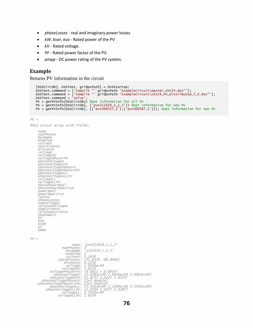
76
phaseLosses - real and imaginary power losses
kW, kvar, kva - Rated power of the PV
kV - Rated voltage.
PF - Rated power factor of the PV.
pmpp - DC power rating of the PV system.
Example
Returns PV information in the circuit
PV = 99x1 struct array with fields: name numPhases busName enabled current coordinates distance voltage voltagePU voltagePhasorPU phaseVoltages phaseVoltagesPU phaseVoltagePhasors phaseVoltagePhasorsPU phaseVoltagesLL phaseVoltagesLLPU voltageLL voltageLLPU phasePowerReal phasePowerReactive powerReal powerReactive losses phaseLosses seqVoltages cplxSeqVoltages seqCurrents cplxSeqCurrents seqPowers kV kVA kVAR pf pmpp PV = name: 'pvn312429_1_2_3' numPhases: 3 busName: 'n312429.1.2.3' enabled: 1 current: 5.3630 coordinates: [31.6376 -80.8964] distance: 6.2216 voltage: 2.0456e+04 voltagePU: 1.0270 voltagePhasorPU: -0.0022 + 0.0053i phaseVoltages: [2.0382e+04 2.0420e+04 2.0565e+04] phaseVoltagesPU: [1.0233 1.0252 1.0325] phaseVoltagePhasors: [1x3 double] phaseVoltagePhasorsPU: [1x3 double] phaseVoltagesLL: [3.5412e+04 3.5388e+04 3.5491e+04] phaseVoltagesLLPU: [1.0264 1.0257 1.0287] voltageLL: 3.5430e+04 voltageLLPU: 1.0270
[DSSCircObj, DSSText, gridpvPath] = DSSStartup; DSSText.command = ['Compile "' gridpvPath 'ExampleCircuit\master_Ckt24.dss"']; DSSText.command = ['Compile "' gridpvPath 'ExampleCircuit\Ckt24_PV_Distributed_7_5.dss"']; DSSText.command = 'solve'; PV = getPVInfo(DSSCircObj) %Get information for all PV PV = getPVInfo(DSSCircObj, {'pvn312429_1_2_3'}) %Get information for one PV PV = getPVInfo(DSSCircObj, [{'pvn300557_3'};{'pvn300587_2'}]); %Get information for two PV
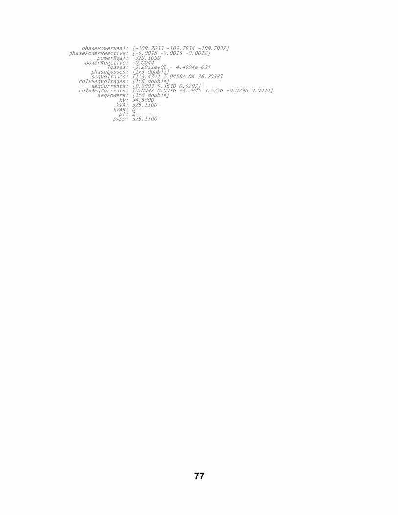
77
phasePowerReal: [-109.7033 -109.7034 -109.7032] phasePowerReactive: [-0.0018 -0.0015 -0.0012] powerReal: -329.1099 powerReactive: -0.0044 losses: -3.2911e+02 - 4.4094e-03i phaseLosses: [1x3 double] seqVoltages: [113.4341 2.0456e+04 36.2038] cplxSeqVoltages: [1x6 double] seqCurrents: [0.0093 5.3630 0.0297] cplxSeqCurrents: [0.0092 0.0016 -4.2845 3.2256 -0.0296 0.0034] seqPowers: [1x6 double] kV: 34.5000 kVA: 329.1100 kVAR: 0 pf: 1 pmpp: 329.1100
78
6.1.10. getTransformerInfo
Gets the information for all transformers in the circuit
Syntax Transformers = getTransformerInfo(DSSCircObj) Transformers = getTransformerInfo(DSSCircObj, transformerNames)
Description
Function to get the information about the transformers in the circuit and return a structure with
the information. If the optional input of transformerNames is filled, the function returns
information for the specified subset of transformers, excluding the miscellaneous parameters
mentioned in the outputs below.
Inputs
DSSCircObj - link to OpenDSS active circuit and command text (from DSSStartup)
transformerNames - optional cell array of transformer names to get information for
Outputs
Transformers is a structure with all the parameters for the transformers in the active circuit.
Fields are:
name - Name of the transformer.
bus1 - Primary bus.
bus2 - Secondary bus.
numPhases - Number of phases associated with the transformer.
enabled - {1|0} indicates whether this element is enabled in the simulation.
bus1PhasePowerReal - 3-element array of the real components of each phase's complex power
at bus 1. Phases that are not present will return 0.
bus1PhasePowerReactive - 3-element array of the imaginary components of each phase's
complex power at bus 1. Phases that are not present will return 0.
bus2PhasePowerReal - 3-element array of the real components of each phase's complex power
at bus 2. Phases that are not present will return 0.
bus2PhasePowerReactive - 3-element array of the imaginary components of each phase's
complex power at bus 2. Phases that are not present will return 0.
bus1PowerReal - Total real component at bus 1 of all present phases.
bus1PowerReactive - Total imaginary component at bus 1 of all present phases.
bus2PowerReal - Total real component at bus 2 of all present phases.
bus2PowerReactive - Total imaginary component at bus 2 of all present phases.
bus1NodeOrder, bus1Coordinates, bus1Distance, bus1PhaseVoltages, bus1PhaseVoltagesPU,
bus1Voltage, bus1VoltagePU, bus1VoltagePhasors, bus1PhaseVoltagesLL,
bus1PhaseVoltagesLLPU, - Information regarding the starting bus. All obtained from the
corresponding fields of the structure returned by getBusInfo when called with 'bus1' as an input.
79
bus2NodeOrder, bus2Coordinates, bus2Distance, bus2PhaseVoltages, bus2PhaseVoltagesPU,
bus2Voltage, bus2VoltagePU, bus2VoltagePhasors, bus2PhaseVoltagePhasorsPU,
bus2PhaseVoltagePhasorsPU, bus2PhaseVoltagesLL, bus2PhaseVoltagesLLPU - Information
regarding the ending bus. All obtained from the corresponding fields of the structure returned
by getBusInfo when called with 'bus2' as an input.
losses - total real and imaginary power losses
phaseLosses - real and imaginary power losses
seqVoltages, cplxVoltages, seqCurrents, cplxSeqCurrents - zero, positive, and negative sequence
voltages and currents magnitude or complex phasors
inputkva - apparent power magnitude coming into the transformer
controlled - Whether or not the transformer is tap-controlled.
kva - Transformer power rating.
XfmrCode - name of the transformer code if one is assigned
wdg1R, wdg1Tap, wdg1minTap, wdg1maxTap, wdg1numTaps, bus1kV, isDelta - properties for
the first winding of the transformer. All properties exist for the wdg2 side as well
Xneut, Rneut, Xhl, Xht, PCTnoLoadLoss - OpenDSS Transformer properties
CTPrimary, delay, forwardBand, forwardR, forwardVreg, forwardX, isInverseTime, _isReversible,
maxTapChange, monitoredBus, PTratio, reverseBand, reverseR, reverseVreg, reverseX, tapDelay,
tapWinding, voltageLimit, winding - OpenDSS properties for the RegControl object for
transformers on which one is present
Example
Returns transformer information in the circuit
Transformers = 843x1 struct array with fields: name bus1 bus2 numPhases enabled bus1PhasePowerReal bus1PhasePowerReactive bus2PhasePowerReal bus2PhasePowerReactive bus1PowerReal bus1PowerReactive bus2PowerReal bus2PowerReactive bus1NodeOrder bus2NodeOrder bus1Voltage bus1VoltagePU bus1PhaseVoltages bus1PhaseVoltagesPU bus1PhaseVoltagePhasors
[DSSCircObj, DSSText, gridpvPath] = DSSStartup; DSSText.command = ['Compile "' gridpvPath 'ExampleCircuit\master_Ckt24.dss"']; DSSText.command = 'solve'; Transformers = getTransformerInfo(DSSCircObj) %Get information for all transformers Transformers = getTransformerInfo(DSSCircObj,DSSCircObj.ActiveCircuit.Transformers.AllNames) %Get information for all transformers Transformers = getTransformerInfo(DSSCircObj, {'05410_g2101ak7700'}) %Get information for one transformer Transformers = getTransformerInfo(DSSCircObj, [{'05410_g2101ah4300'};{'05410_g2101ae2300'}]); %Get information for two transformers
80
bus1PhaseVoltagePhasorsPU bus1PhaseVoltagesLL bus1PhaseVoltagesLLPU bus1VoltageLL bus1VoltageLLPU bus2Voltage bus2VoltagePU bus2PhaseVoltages bus2PhaseVoltagesPU bus2PhaseVoltagePhasors bus2PhaseVoltagePhasorsPU bus2PhaseVoltagesLL bus2PhaseVoltagesLLPU bus2VoltageLL bus2VoltageLLPU bus1Distance bus2Distance losses phaseLosses seqVoltages cplxSeqVoltages seqCurrents cplxSeqCurrents seqPower inputkva controlled kva XfmrCode wdg1R wdg1Tap wdg1minTap wdg1maxTap wdg1numTaps bus1kV Xneut Rneut wdg1IsDelta Xhl Xht bus2kV wdg2R wdg2Tap wdg2minTap wdg2maxTap wdg2numTaps wdg2IsDelta PCTloadLoss PCTnoLoadLoss controller CTPrimary delay forwardBand forwardR forwardVreg forwardX isInverseTime isReversible maxTapChange monitoredBus PTratio reverseBand reverseR reverseVreg reverseX tapDelay tapWinding voltageLimit winding Transformers = 843x1 struct array with fields: name bus1 bus2 numPhases enabled bus1PhasePowerReal bus1PhasePowerReactive bus2PhasePowerReal bus2PhasePowerReactive bus1PowerReal bus1PowerReactive bus2PowerReal bus2PowerReactive bus1NodeOrder bus2NodeOrder bus1Voltage
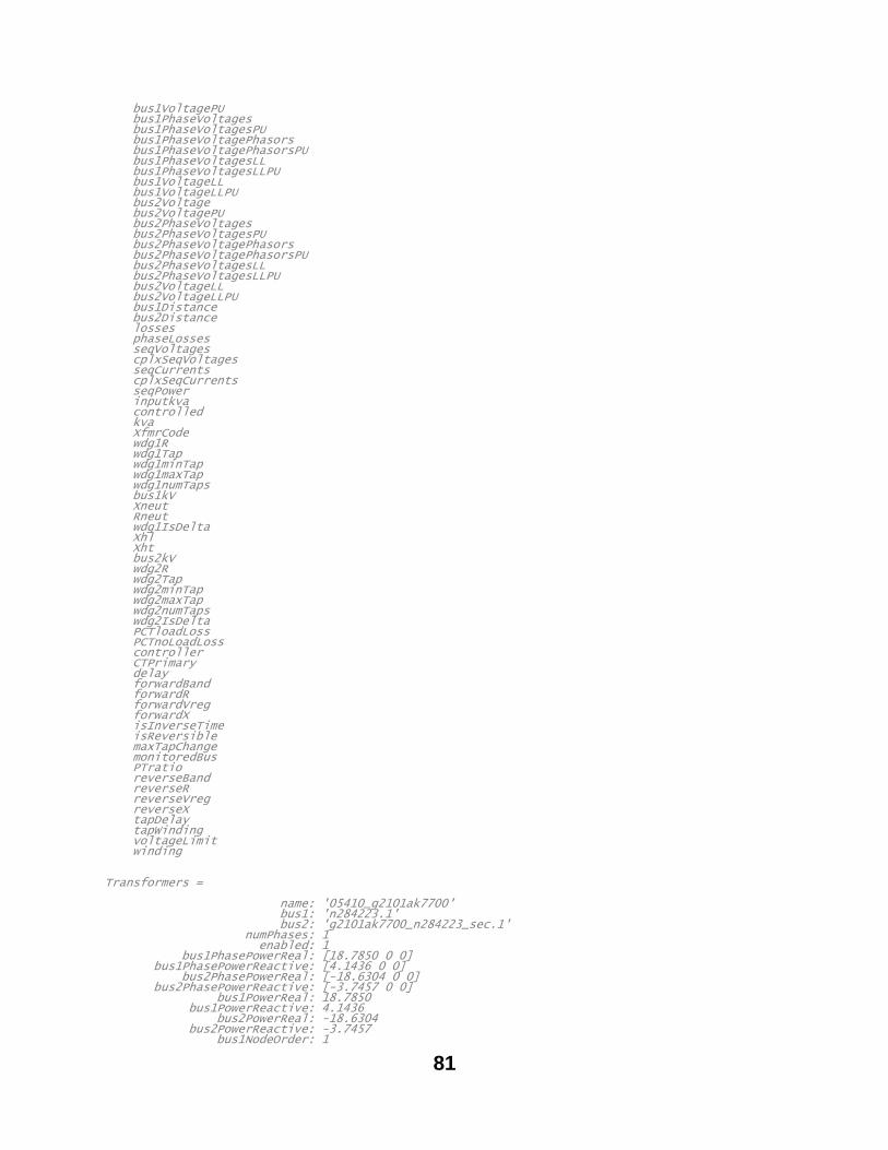
81
bus1VoltagePU bus1PhaseVoltages bus1PhaseVoltagesPU bus1PhaseVoltagePhasors bus1PhaseVoltagePhasorsPU bus1PhaseVoltagesLL bus1PhaseVoltagesLLPU bus1VoltageLL bus1VoltageLLPU bus2Voltage bus2VoltagePU bus2PhaseVoltages bus2PhaseVoltagesPU bus2PhaseVoltagePhasors bus2PhaseVoltagePhasorsPU bus2PhaseVoltagesLL bus2PhaseVoltagesLLPU bus2VoltageLL bus2VoltageLLPU bus1Distance bus2Distance losses phaseLosses seqVoltages cplxSeqVoltages seqCurrents cplxSeqCurrents seqPower inputkva controlled kva XfmrCode wdg1R wdg1Tap wdg1minTap wdg1maxTap wdg1numTaps bus1kV Xneut Rneut wdg1IsDelta Xhl Xht bus2kV wdg2R wdg2Tap wdg2minTap wdg2maxTap wdg2numTaps wdg2IsDelta PCTloadLoss PCTnoLoadLoss controller CTPrimary delay forwardBand forwardR forwardVreg forwardX isInverseTime isReversible maxTapChange monitoredBus PTratio reverseBand reverseR reverseVreg reverseX tapDelay tapWinding voltageLimit winding Transformers = name: '05410_g2101ak7700' bus1: 'n284223.1' bus2: 'g2101ak7700_n284223_sec.1' numPhases: 1 enabled: 1 bus1PhasePowerReal: [18.7850 0 0] bus1PhasePowerReactive: [4.1436 0 0] bus2PhasePowerReal: [-18.6304 0 0] bus2PhasePowerReactive: [-3.7457 0 0] bus1PowerReal: 18.7850 bus1PowerReactive: 4.1436 bus2PowerReal: -18.6304 bus2PowerReactive: -3.7457 bus1NodeOrder: 1
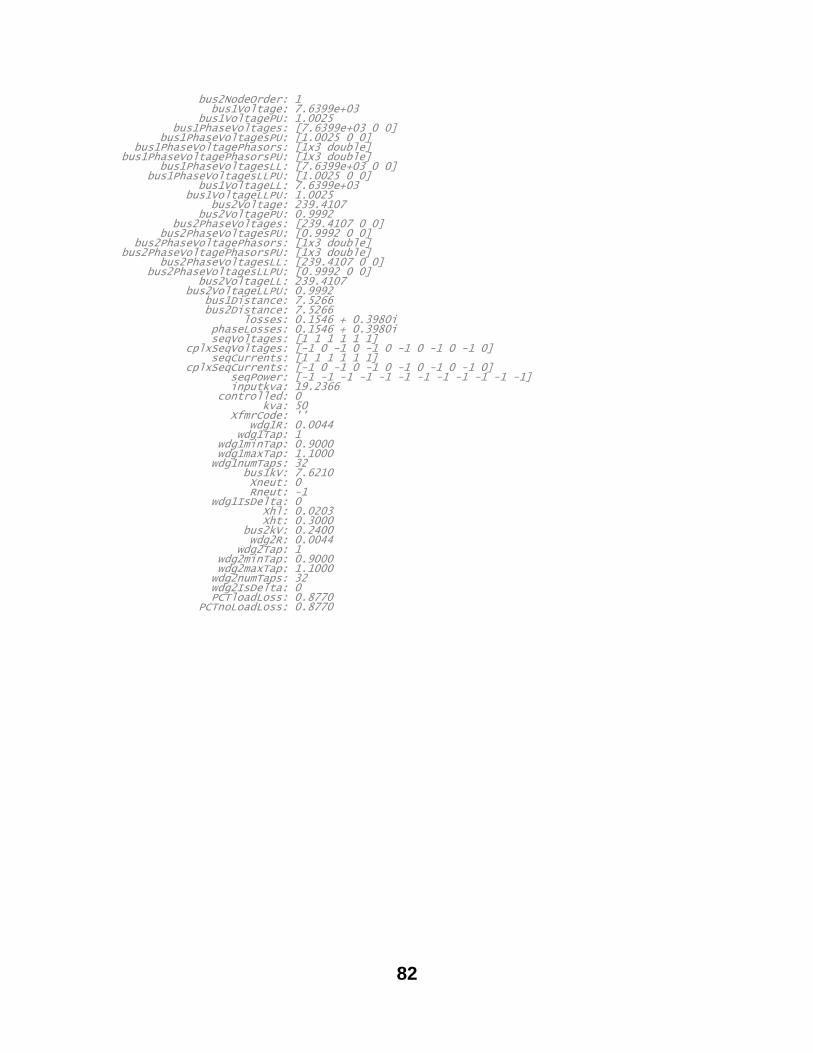
82
bus2NodeOrder: 1 bus1Voltage: 7.6399e+03 bus1VoltagePU: 1.0025 bus1PhaseVoltages: [7.6399e+03 0 0] bus1PhaseVoltagesPU: [1.0025 0 0] bus1PhaseVoltagePhasors: [1x3 double] bus1PhaseVoltagePhasorsPU: [1x3 double] bus1PhaseVoltagesLL: [7.6399e+03 0 0] bus1PhaseVoltagesLLPU: [1.0025 0 0] bus1VoltageLL: 7.6399e+03 bus1VoltageLLPU: 1.0025 bus2Voltage: 239.4107 bus2VoltagePU: 0.9992 bus2PhaseVoltages: [239.4107 0 0] bus2PhaseVoltagesPU: [0.9992 0 0] bus2PhaseVoltagePhasors: [1x3 double] bus2PhaseVoltagePhasorsPU: [1x3 double] bus2PhaseVoltagesLL: [239.4107 0 0] bus2PhaseVoltagesLLPU: [0.9992 0 0] bus2VoltageLL: 239.4107 bus2VoltageLLPU: 0.9992 bus1Distance: 7.5266 bus2Distance: 7.5266 losses: 0.1546 + 0.3980i phaseLosses: 0.1546 + 0.3980i seqVoltages: [1 1 1 1 1 1] cplxSeqVoltages: [-1 0 -1 0 -1 0 -1 0 -1 0 -1 0] seqCurrents: [1 1 1 1 1 1] cplxSeqCurrents: [-1 0 -1 0 -1 0 -1 0 -1 0 -1 0] seqPower: [-1 -1 -1 -1 -1 -1 -1 -1 -1 -1 -1 -1] inputkva: 19.2366 controlled: 0 kva: 50 XfmrCode: '' wdg1R: 0.0044 wdg1Tap: 1 wdg1minTap: 0.9000 wdg1maxTap: 1.1000 wdg1numTaps: 32 bus1kV: 7.6210 Xneut: 0 Rneut: -1 wdg1IsDelta: 0 Xhl: 0.0203 Xht: 0.3000 bus2kV: 0.2400 wdg2R: 0.0044 wdg2Tap: 1 wdg2minTap: 0.9000 wdg2maxTap: 1.1000 wdg2numTaps: 32 wdg2IsDelta: 0 PCTloadLoss: 0.8770 PCTnoLoadLoss: 0.8770
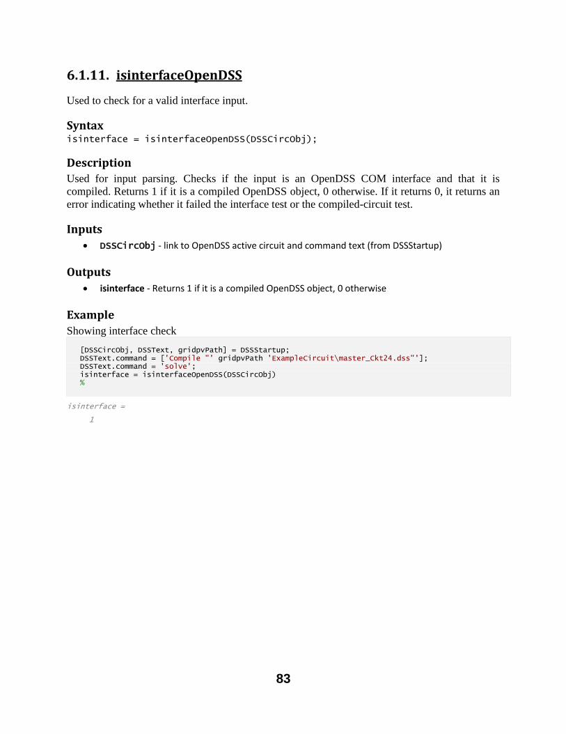
83
6.1.11. isinterfaceOpenDSS
Used to check for a valid interface input.
Syntax isinterface = isinterfaceOpenDSS(DSSCircObj);
Description
Used for input parsing. Checks if the input is an OpenDSS COM interface and that it is
compiled. Returns 1 if it is a compiled OpenDSS object, 0 otherwise. If it returns 0, it returns an
error indicating whether it failed the interface test or the compiled-circuit test.
Inputs
DSSCircObj - link to OpenDSS active circuit and command text (from DSSStartup)
Outputs
isinterface - Returns 1 if it is a compiled OpenDSS object, 0 otherwise
Example
Showing interface check
isinterface = 1
[DSSCircObj, DSSText, gridpvPath] = DSSStartup; DSSText.command = ['Compile "' gridpvPath 'ExampleCircuit\master_Ckt24.dss"']; DSSText.command = 'solve'; isinterface = isinterfaceOpenDSS(DSSCircObj) %
84
6.2. CIRCUIT ANALYSIS FUNCTIONS
Certain pieces of the circuit analysis can better be performed in MATLAB. OpenDSS solves the
power flow and returns the state of the system, but custom queries about features of the circuit
can be accomplished in MATLAB.
Function List
circuitCheck - Used to error-check the circuit for any obvious abnormalities
findDownstreamBuses - Finds all buses downstream of the busName
findHighestImpedanceBus - Finds the highest impedance bus for each phase to the source bus
findLongestDistanceBus - Finds the bus for each phase that is farthest distance away
findSubstationLocation - Locates the substation coordinates
findUpstreamBuses - Finds all buses upstream of the busName
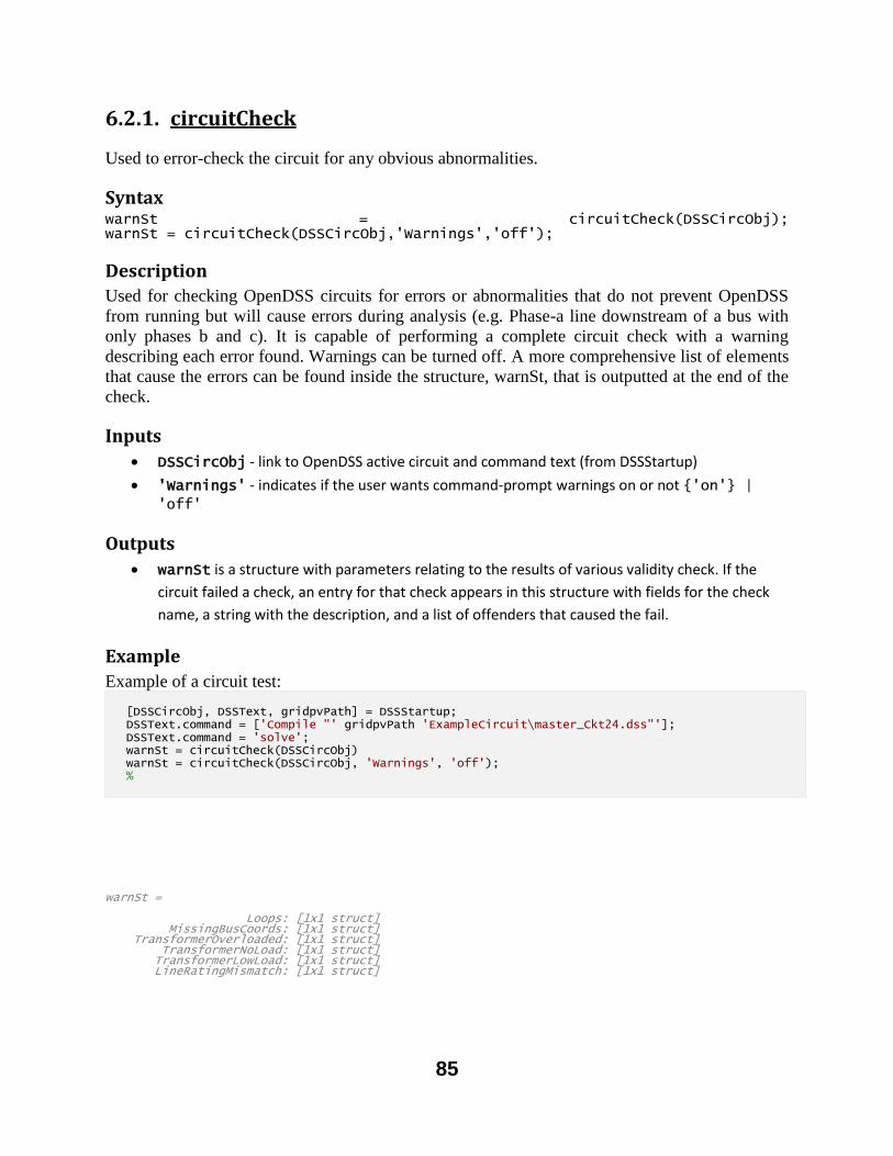
85
6.2.1. circuitCheck
Used to error-check the circuit for any obvious abnormalities.
Syntax warnSt = circuitCheck(DSSCircObj); warnSt = circuitCheck(DSSCircObj,'Warnings','off');
Description
Used for checking OpenDSS circuits for errors or abnormalities that do not prevent OpenDSS
from running but will cause errors during analysis (e.g. Phase-a line downstream of a bus with
only phases b and c). It is capable of performing a complete circuit check with a warning
describing each error found. Warnings can be turned off. A more comprehensive list of elements
that cause the errors can be found inside the structure, warnSt, that is outputted at the end of the
check.
Inputs
DSSCircObj - link to OpenDSS active circuit and command text (from DSSStartup)
'Warnings' - indicates if the user wants command-prompt warnings on or not {'on'} | 'off'
Outputs
warnSt is a structure with parameters relating to the results of various validity check. If the
circuit failed a check, an entry for that check appears in this structure with fields for the check
name, a string with the description, and a list of offenders that caused the fail.
Example
Example of a circuit test:
warnSt = Loops: [1x1 struct] MissingBusCoords: [1x1 struct] TransformerOverloaded: [1x1 struct] TransformerNoLoad: [1x1 struct] TransformerLowLoad: [1x1 struct] LineRatingMismatch: [1x1 struct]
[DSSCircObj, DSSText, gridpvPath] = DSSStartup; DSSText.command = ['Compile "' gridpvPath 'ExampleCircuit\master_Ckt24.dss"']; DSSText.command = 'solve'; warnSt = circuitCheck(DSSCircObj) warnSt = circuitCheck(DSSCircObj, 'Warnings', 'off'); %
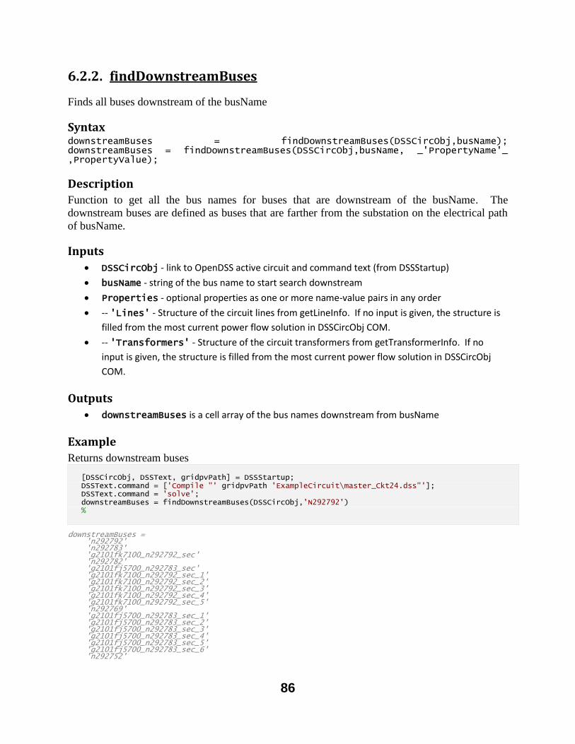
86
6.2.2. findDownstreamBuses
Finds all buses downstream of the busName
Syntax downstreamBuses = findDownstreamBuses(DSSCircObj,busName); downstreamBuses = findDownstreamBuses(DSSCircObj,busName, _'PropertyName'_ ,PropertyValue);
Description
Function to get all the bus names for buses that are downstream of the busName. The
downstream buses are defined as buses that are farther from the substation on the electrical path
of busName.
Inputs
DSSCircObj - link to OpenDSS active circuit and command text (from DSSStartup)
busName - string of the bus name to start search downstream
Properties - optional properties as one or more name-value pairs in any order
-- 'Lines' - Structure of the circuit lines from getLineInfo. If no input is given, the structure is
filled from the most current power flow solution in DSSCircObj COM.
-- 'Transformers' - Structure of the circuit transformers from getTransformerInfo. If no
input is given, the structure is filled from the most current power flow solution in DSSCircObj
COM.
Outputs
downstreamBuses is a cell array of the bus names downstream from busName
Example
Returns downstream buses
downstreamBuses = 'n292792' 'n292783' 'g2101fk7100_n292792_sec' 'n292782' 'g2101fj5700_n292783_sec' 'g2101fk7100_n292792_sec_1' 'g2101fk7100_n292792_sec_2' 'g2101fk7100_n292792_sec_3' 'g2101fk7100_n292792_sec_4' 'g2101fk7100_n292792_sec_5' 'n292769' 'g2101fj5700_n292783_sec_1' 'g2101fj5700_n292783_sec_2' 'g2101fj5700_n292783_sec_3' 'g2101fj5700_n292783_sec_4' 'g2101fj5700_n292783_sec_5' 'g2101fj5700_n292783_sec_6' 'n292752'
[DSSCircObj, DSSText, gridpvPath] = DSSStartup; DSSText.command = ['Compile "' gridpvPath 'ExampleCircuit\master_Ckt24.dss"']; DSSText.command = 'solve'; downstreamBuses = findDownstreamBuses(DSSCircObj,'N292792') %
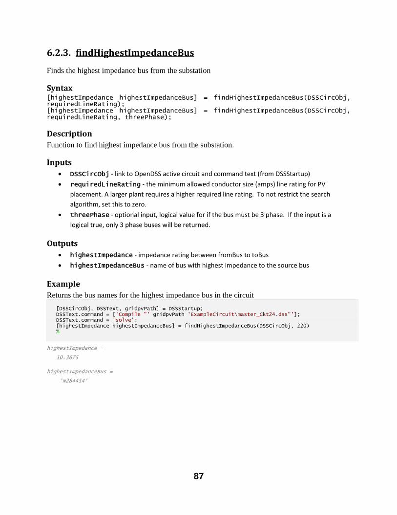
87
6.2.3. findHighestImpedanceBus
Finds the highest impedance bus from the substation
Syntax [highestImpedance highestImpedanceBus] = findHighestImpedanceBus(DSSCircObj, requiredLineRating); [highestImpedance highestImpedanceBus] = findHighestImpedanceBus(DSSCircObj, requiredLineRating, threePhase);
Description
Function to find highest impedance bus from the substation.
Inputs
DSSCircObj - link to OpenDSS active circuit and command text (from DSSStartup)
requiredLineRating - the minimum allowed conductor size (amps) line rating for PV
placement. A larger plant requires a higher required line rating. To not restrict the search
algorithm, set this to zero.
threePhase - optional input, logical value for if the bus must be 3 phase. If the input is a
logical true, only 3 phase buses will be returned.
Outputs
highestImpedance - impedance rating between fromBus to toBus
highestImpedanceBus - name of bus with highest impedance to the source bus
Example
Returns the bus names for the highest impedance bus in the circuit
highestImpedance = 10.3675 highestImpedanceBus = 'N284454'
[DSSCircObj, DSSText, gridpvPath] = DSSStartup; DSSText.command = ['Compile "' gridpvPath 'ExampleCircuit\master_Ckt24.dss"']; DSSText.command = 'solve'; [highestImpedance highestImpedanceBus] = findHighestImpedanceBus(DSSCircObj, 220) %
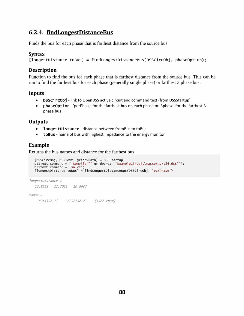
88
6.2.4. findLongestDistanceBus
Finds the bus for each phase that is farthest distance from the source bus
Syntax [longestDistance toBus] = findLongestDistanceBus(DSSCircObj, phaseOption);
Description
Function to find the bus for each phase that is farthest distance from the source bus. This can be
run to find the farthest bus for each phase (generally single phase) or farthest 3 phase bus.
Inputs
DSSCircObj - link to OpenDSS active circuit and command text (from DSSStartup)
phaseOption - 'perPhase' for the farthest bus on each phase or '3phase' for the farthest 3 phase bus
Outputs
longestDistance - distance between fromBus to toBus
toBus - name of bus with highest impedance to the energy monitor
Example
Returns the bus names and distance for the farthest bus
longestDistance = 12.8993 11.2051 10.9983 toBus = 'n284397.1' 'n292752.2' [1x27 char]
[DSSCircObj, DSSText, gridpvPath] = DSSStartup; DSSText.command = ['Compile "' gridpvPath 'ExampleCircuit\master_Ckt24.dss"']; DSSText.command = 'solve'; [longestDistance toBus] = findLongestDistanceBus(DSSCircObj, 'perPhase')
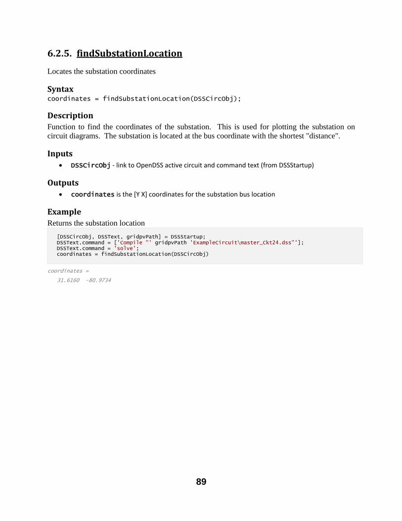
89
6.2.5. findSubstationLocation
Locates the substation coordinates
Syntax coordinates = findSubstationLocation(DSSCircObj);
Description
Function to find the coordinates of the substation. This is used for plotting the substation on
circuit diagrams. The substation is located at the bus coordinate with the shortest "distance".
Inputs
DSSCircObj - link to OpenDSS active circuit and command text (from DSSStartup)
Outputs
coordinates is the [Y X] coordinates for the substation bus location
Example
Returns the substation location
coordinates = 31.6160 -80.9734
[DSSCircObj, DSSText, gridpvPath] = DSSStartup; DSSText.command = ['Compile "' gridpvPath 'ExampleCircuit\master_Ckt24.dss"']; DSSText.command = 'solve'; coordinates = findSubstationLocation(DSSCircObj)
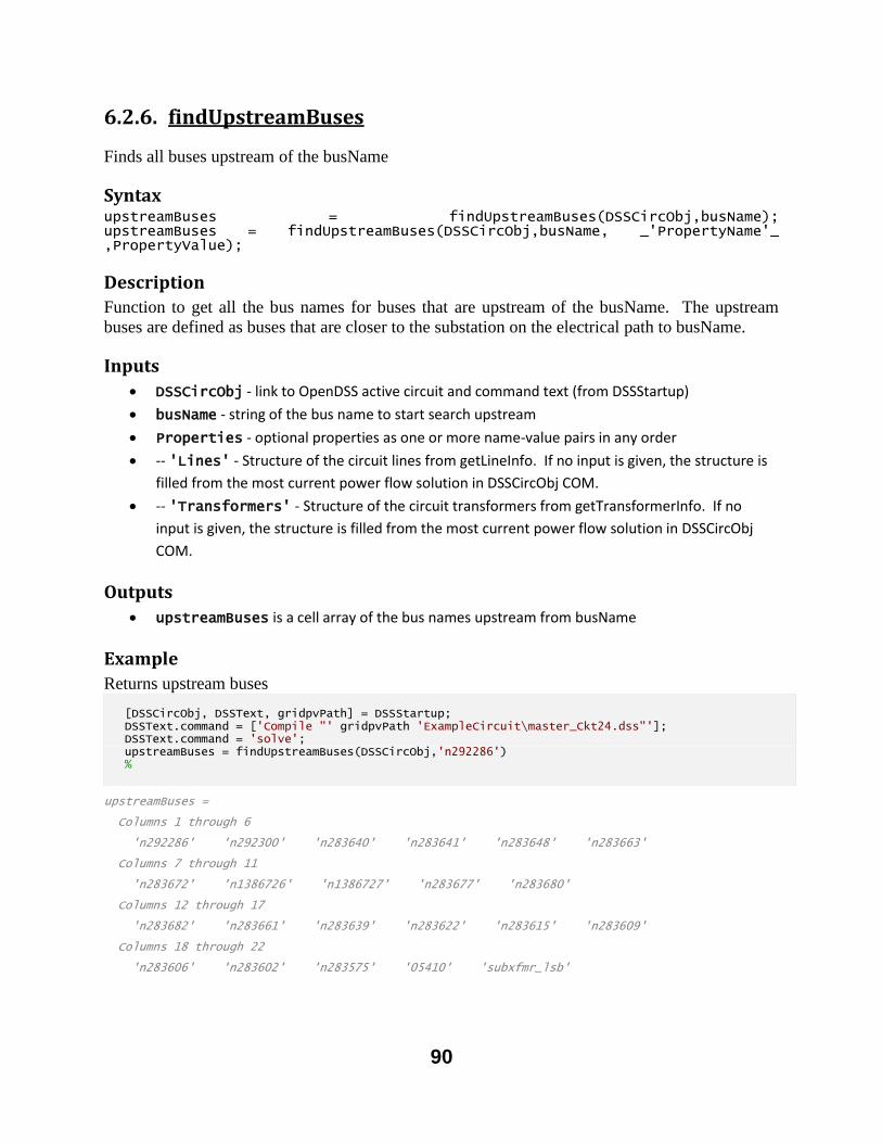
90
6.2.6. findUpstreamBuses
Finds all buses upstream of the busName
Syntax upstreamBuses = findUpstreamBuses(DSSCircObj,busName); upstreamBuses = findUpstreamBuses(DSSCircObj,busName, _'PropertyName'_ ,PropertyValue);
Description
Function to get all the bus names for buses that are upstream of the busName. The upstream
buses are defined as buses that are closer to the substation on the electrical path to busName.
Inputs
DSSCircObj - link to OpenDSS active circuit and command text (from DSSStartup)
busName - string of the bus name to start search upstream
Properties - optional properties as one or more name-value pairs in any order
-- 'Lines' - Structure of the circuit lines from getLineInfo. If no input is given, the structure is
filled from the most current power flow solution in DSSCircObj COM.
-- 'Transformers' - Structure of the circuit transformers from getTransformerInfo. If no
input is given, the structure is filled from the most current power flow solution in DSSCircObj
COM.
Outputs
upstreamBuses is a cell array of the bus names upstream from busName
Example
Returns upstream buses
upstreamBuses = Columns 1 through 6 'n292286' 'n292300' 'n283640' 'n283641' 'n283648' 'n283663' Columns 7 through 11 'n283672' 'n1386726' 'n1386727' 'n283677' 'n283680' Columns 12 through 17 'n283682' 'n283661' 'n283639' 'n283622' 'n283615' 'n283609' Columns 18 through 22 'n283606' 'n283602' 'n283575' '05410' 'subxfmr_lsb'
[DSSCircObj, DSSText, gridpvPath] = DSSStartup; DSSText.command = ['Compile "' gridpvPath 'ExampleCircuit\master_Ckt24.dss"']; DSSText.command = 'solve'; upstreamBuses = findUpstreamBuses(DSSCircObj,'n292286') %
91
6.3. PLOTTING FUNCTIONS
These functions create plots in MATLAB from the OpenDSS system. While some of these plots
can be created directly in OpenDSS, plotting in MATLAB provides more customization and
functionality. These plot functions can be called at any time during an OpenDSS simulation, and
they will plot the current state of the OpenDSS feeder. If there are any solar generators in the
simulation, the functions will identify the location and mark the PV in the plots.
Function List
plotAmpProfile - Plots the line currents profile and line rating vs. distance
plotCircuitLines - Plots the feeder circuit diagram
plotCircuitLinesOptions - GUI for providing options for how to plot the feeder circuit diagram
plotKVARProfile - Plots the feeder profile for the kVAR power flow on the lines
plotKWProfile - Plots the feeder profile for the kW power flow on the lines
plotMonitor - Plots a monitor from the simulation
plotVoltageProfile - Plots the voltage profile for the feeder (spider plot)
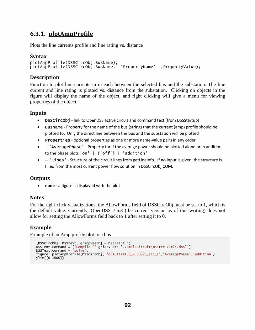
92
6.3.1. plotAmpProfile
Plots the line currents profile and line rating vs. distance
Syntax plotAmpProfile(DSSCircObj,BusName); plotAmpProfile(DSSCircObj,BusName, _'PropertyName'_ ,PropertyValue);
Description
Function to plot line currents in in each between the selected bus and the substation. The line
current and line rating is plotted vs. distance from the substation. Clicking on objects in the
figure will display the name of the object, and right clicking will give a menu for viewing
properties of the object.
Inputs
DSSCircObj - link to OpenDSS active circuit and command text (from DSSStartup)
BusName - Property for the name of the bus (string) that the current (amp) profile should be
plotted to. Only the direct line between the bus and the substation will be plotted
Properties - optional properties as one or more name-value pairs in any order
-- 'AveragePhase' - Property for if the average power should be plotted alone or in addition
to the phase plots 'on' | {'off'} | 'addition'
-- 'Lines' - Structure of the circuit lines from getLineInfo. If no input is given, the structure is
filled from the most current power flow solution in DSSCircObj COM.
Outputs
none - a figure is displayed with the plot
Notes
For the right-click visualizations, the AllowForms field of DSSCircObj must be set to 1, which is
the default value. Currently, OpenDSS 7.6.3 (the current version as of this writing) does not
allow for setting the AllowForms field back to 1 after setting it to 0.
Example
Example of an Amp profile plot to a bus
[DSSCircObj, DSSText, gridpvPath] = DSSStartup; DSSText.command = ['Compile "' gridpvPath 'ExampleCircuit\master_Ckt24.dss"']; DSSText.command = 'solve'; figure; plotAmpProfile(DSSCircObj, 'G2101JK1400_N300995_sec_1','AveragePhase','addition') ylim([0 1000])

93
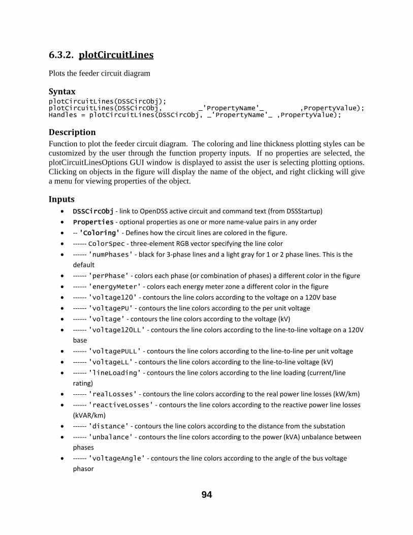
94
6.3.2. plotCircuitLines
Plots the feeder circuit diagram
Syntax plotCircuitLines(DSSCircObj); plotCircuitLines(DSSCircObj, _'PropertyName'_ ,PropertyValue); Handles = plotCircuitLines(DSSCircObj, _'PropertyName'_ ,PropertyValue);
Description
Function to plot the feeder circuit diagram. The coloring and line thickness plotting styles can be
customized by the user through the function property inputs. If no properties are selected, the
plotCircuitLinesOptions GUI window is displayed to assist the user is selecting plotting options.
Clicking on objects in the figure will display the name of the object, and right clicking will give
a menu for viewing properties of the object.
Inputs
DSSCircObj - link to OpenDSS active circuit and command text (from DSSStartup)
Properties - optional properties as one or more name-value pairs in any order
-- 'Coloring' - Defines how the circuit lines are colored in the figure.
------ ColorSpec - three-element RGB vector specifying the line color
------ 'numPhases' - black for 3-phase lines and a light gray for 1 or 2 phase lines. This is the
default
------ 'perPhase' - colors each phase (or combination of phases) a different color in the figure
------ 'energyMeter' - colors each energy meter zone a different color in the figure
------ 'voltage120' - contours the line colors according to the voltage on a 120V base
------ 'voltagePU' - contours the line colors according to the per unit voltage
------ 'voltage' - contours the line colors according to the voltage (kV)
------ 'voltage120LL' - contours the line colors according to the line-to-line voltage on a 120V
base
------ 'voltagePULL' - contours the line colors according to the line-to-line per unit voltage
------ 'voltageLL' - contours the line colors according to the line-to-line voltage (kV)
------ 'lineLoading' - contours the line colors according to the line loading (current/line
rating)
------ 'realLosses' - contours the line colors according to the real power line losses (kW/km)
------ 'reactiveLosses' - contours the line colors according to the reactive power line losses
(kVAR/km)
------ 'distance' - contours the line colors according to the distance from the substation
------ 'unbalance' - contours the line colors according to the power (kVA) unbalance between
phases
------ 'voltageAngle' - contours the line colors according to the angle of the bus voltage
phasor
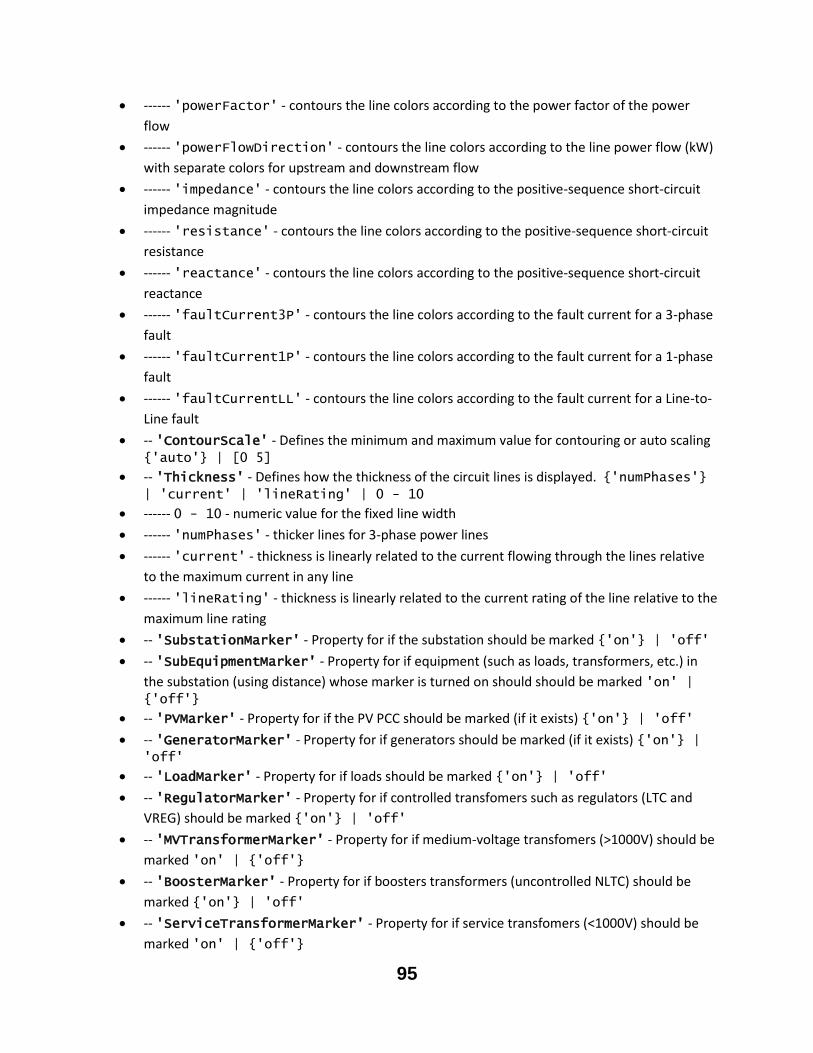
95
------ 'powerFactor' - contours the line colors according to the power factor of the power
flow
------ 'powerFlowDirection' - contours the line colors according to the line power flow (kW)
with separate colors for upstream and downstream flow
------ 'impedance' - contours the line colors according to the positive-sequence short-circuit
impedance magnitude
------ 'resistance' - contours the line colors according to the positive-sequence short-circuit
resistance
------ 'reactance' - contours the line colors according to the positive-sequence short-circuit
reactance
------ 'faultCurrent3P' - contours the line colors according to the fault current for a 3-phase
fault
------ 'faultCurrent1P' - contours the line colors according to the fault current for a 1-phase
fault
------ 'faultCurrentLL' - contours the line colors according to the fault current for a Line-to-
Line fault
-- 'ContourScale' - Defines the minimum and maximum value for contouring or auto scaling {'auto'} | [0 5]
-- 'Thickness' - Defines how the thickness of the circuit lines is displayed. {'numPhases'} | 'current' | 'lineRating' | 0 - 10
------ 0 - 10 - numeric value for the fixed line width
------ 'numPhases' - thicker lines for 3-phase power lines
------ 'current' - thickness is linearly related to the current flowing through the lines relative
to the maximum current in any line
------ 'lineRating' - thickness is linearly related to the current rating of the line relative to the
maximum line rating
-- 'SubstationMarker' - Property for if the substation should be marked {'on'} | 'off'
-- 'SubEquipmentMarker' - Property for if equipment (such as loads, transformers, etc.) in
the substation (using distance) whose marker is turned on should should be marked 'on' | {'off'}
-- 'PVMarker' - Property for if the PV PCC should be marked (if it exists) {'on'} | 'off'
-- 'GeneratorMarker' - Property for if generators should be marked (if it exists) {'on'} | 'off'
-- 'LoadMarker' - Property for if loads should be marked {'on'} | 'off'
-- 'RegulatorMarker' - Property for if controlled transfomers such as regulators (LTC and
VREG) should be marked {'on'} | 'off'
-- 'MVTransformerMarker' - Property for if medium-voltage transfomers (>1000V) should be
marked 'on' | {'off'}
-- 'BoosterMarker' - Property for if boosters transformers (uncontrolled NLTC) should be
marked {'on'} | 'off'
-- 'ServiceTransformerMarker' - Property for if service transfomers (<1000V) should be
marked 'on' | {'off'}
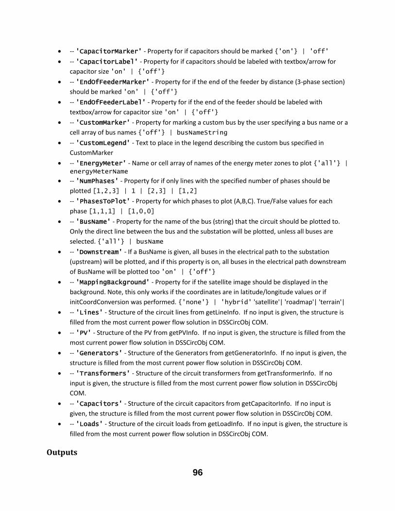
96
-- 'CapacitorMarker' - Property for if capacitors should be marked {'on'} | 'off'
-- 'CapacitorLabel' - Property for if capacitors should be labeled with textbox/arrow for
capacitor size 'on' | {'off'}
-- 'EndOfFeederMarker' - Property for if the end of the feeder by distance (3-phase section)
should be marked 'on' | {'off'}
-- 'EndOfFeederLabel' - Property for if the end of the feeder should be labeled with
textbox/arrow for capacitor size 'on' | {'off'}
-- 'CustomMarker' - Property for marking a custom bus by the user specifying a bus name or a
cell array of bus names {'off'} | busNameString
-- 'CustomLegend' - Text to place in the legend describing the custom bus specified in
CustomMarker
-- 'EnergyMeter' - Name or cell array of names of the energy meter zones to plot {'all'} | energyMeterName
-- 'NumPhases' - Property for if only lines with the specified number of phases should be
plotted [1,2,3] | 1 | [2,3] | [1,2]
-- 'PhasesToPlot' - Property for which phases to plot (A,B,C). True/False values for each
phase [1,1,1] | [1,0,0]
-- 'BusName' - Property for the name of the bus (string) that the circuit should be plotted to.
Only the direct line between the bus and the substation will be plotted, unless all buses are
selected. {'all'} | busName
-- 'Downstream' - If a BusName is given, all buses in the electrical path to the substation
(upstream) will be plotted, and if this property is on, all buses in the electrical path downstream
of BusName will be plotted too 'on' | {'off'}
-- 'MappingBackground' - Property for if the satellite image should be displayed in the
background. Note, this only works if the coordinates are in latitude/longitude values or if
initCoordConversion was performed. {'none'} | 'hybrid' 'satellite'| 'roadmap'| 'terrain'|
-- 'Lines' - Structure of the circuit lines from getLineInfo. If no input is given, the structure is
filled from the most current power flow solution in DSSCircObj COM.
-- 'PV' - Structure of the PV from getPVInfo. If no input is given, the structure is filled from the
most current power flow solution in DSSCircObj COM.
-- 'Generators' - Structure of the Generators from getGeneratorInfo. If no input is given, the
structure is filled from the most current power flow solution in DSSCircObj COM.
-- 'Transformers' - Structure of the circuit transformers from getTransformerInfo. If no
input is given, the structure is filled from the most current power flow solution in DSSCircObj
COM.
-- 'Capacitors' - Structure of the circuit capacitors from getCapacitorInfo. If no input is
given, the structure is filled from the most current power flow solution in DSSCircObj COM.
-- 'Loads' - Structure of the circuit loads from getLoadInfo. If no input is given, the structure is
filled from the most current power flow solution in DSSCircObj COM.
Outputs
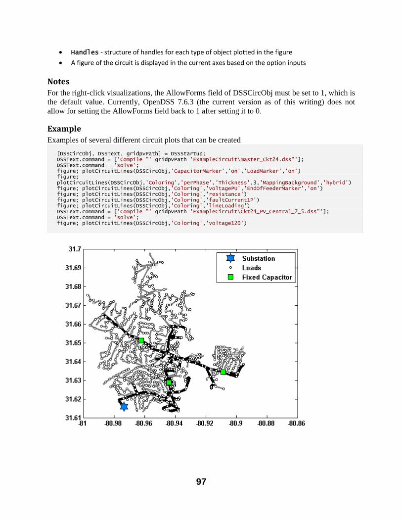
97
Handles - structure of handles for each type of object plotted in the figure
A figure of the circuit is displayed in the current axes based on the option inputs
Notes
For the right-click visualizations, the AllowForms field of DSSCircObj must be set to 1, which is
the default value. Currently, OpenDSS 7.6.3 (the current version as of this writing) does not
allow for setting the AllowForms field back to 1 after setting it to 0.
Example
Examples of several different circuit plots that can be created
[DSSCircObj, DSSText, gridpvPath] = DSSStartup; DSSText.command = ['Compile "' gridpvPath 'ExampleCircuit\master_Ckt24.dss"']; DSSText.command = 'solve'; figure; plotCircuitLines(DSSCircObj,'CapacitorMarker','on','LoadMarker','on') figure; plotCircuitLines(DSSCircObj,'Coloring','perPhase','Thickness',3,'MappingBackground','hybrid') figure; plotCircuitLines(DSSCircObj,'Coloring','voltagePU','EndOfFeederMarker','on') figure; plotCircuitLines(DSSCircObj,'Coloring','resistance') figure; plotCircuitLines(DSSCircObj,'Coloring','faultCurrent1P') figure; plotCircuitLines(DSSCircObj,'Coloring','lineLoading') DSSText.command = ['Compile "' gridpvPath 'ExampleCircuit\Ckt24_PV_Central_7_5.dss"']; DSSText.command = 'solve'; figure; plotCircuitLines(DSSCircObj,'Coloring','voltage120')
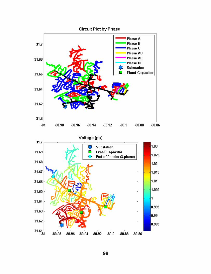
98

99
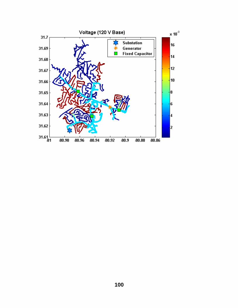
100
101
6.3.3. plotCircuitLinesOptions
GUI for providing options for how to plot the feeder circuit diagram
Syntax plotCircuitLinesOptions(DSSCircObj);
Description
plotCircuitLines plots the feeder circuit diagram and has many different input argument
parameters for changing coloring, line thickness, background, etc. This function provides a GUI
for selecting the plotting styles for plotCircuitLines instead of through text arguments. This
function can be called directly with the OpenDSS circuit object, or plotCircuitLines.m will call
this function if no input arguments were selected.
Inputs
DSSCircObj - link to OpenDSS active circuit and command text (from DSSStartup)
Outputs
none - a figure of the circuit is displayed based on the option inputs
Example
Examples of calling the GUI for plotCircuitLinesOptions
[DSSCircObj, DSSText, gridpvPath] = DSSStartup; DSSText.command = ['Compile "' gridpvPath 'ExampleCircuit\master_Ckt24.dss"']; DSSText.command = 'solve'; figure; plotCircuitLinesOptions(DSSCircObj) %
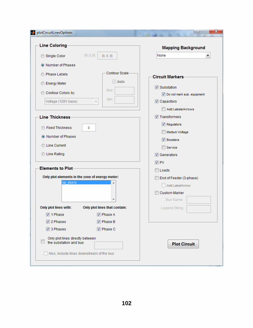
102
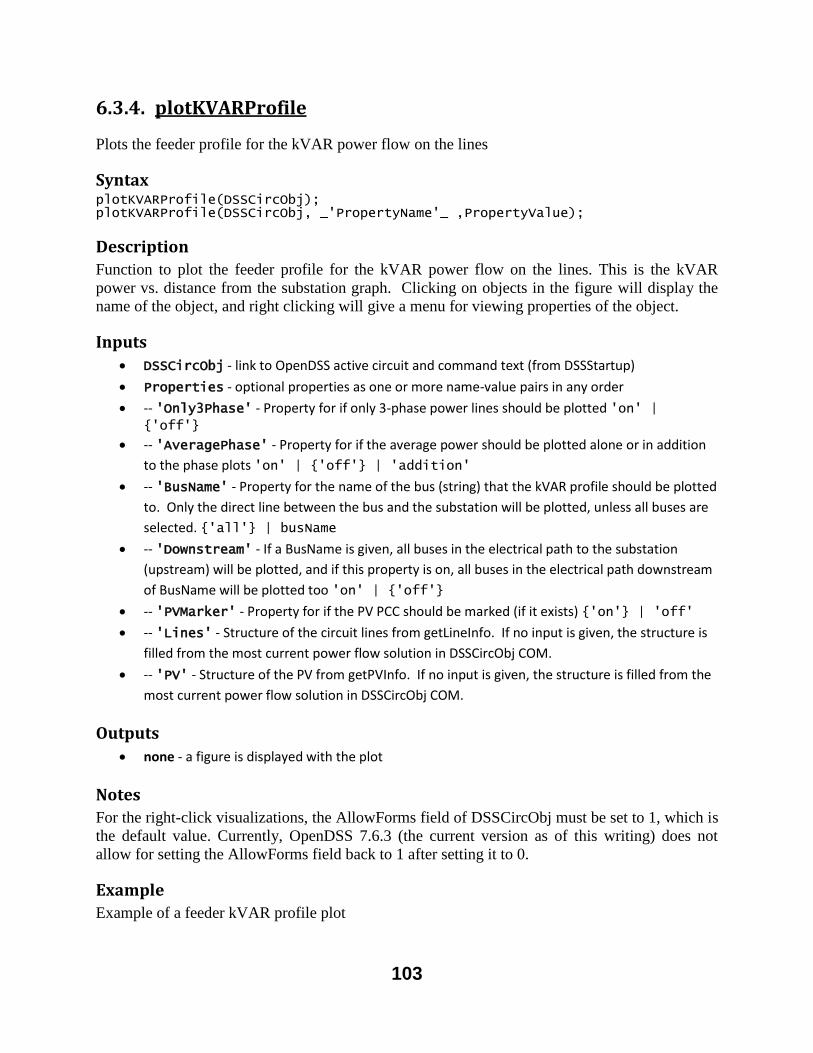
103
6.3.4. plotKVARProfile
Plots the feeder profile for the kVAR power flow on the lines
Syntax plotKVARProfile(DSSCircObj); plotKVARProfile(DSSCircObj, _'PropertyName'_ ,PropertyValue);
Description
Function to plot the feeder profile for the kVAR power flow on the lines. This is the kVAR
power vs. distance from the substation graph. Clicking on objects in the figure will display the
name of the object, and right clicking will give a menu for viewing properties of the object.
Inputs
DSSCircObj - link to OpenDSS active circuit and command text (from DSSStartup)
Properties - optional properties as one or more name-value pairs in any order
-- 'Only3Phase' - Property for if only 3-phase power lines should be plotted 'on' | {'off'}
-- 'AveragePhase' - Property for if the average power should be plotted alone or in addition
to the phase plots 'on' | {'off'} | 'addition'
-- 'BusName' - Property for the name of the bus (string) that the kVAR profile should be plotted
to. Only the direct line between the bus and the substation will be plotted, unless all buses are
selected. {'all'} | busName
-- 'Downstream' - If a BusName is given, all buses in the electrical path to the substation
(upstream) will be plotted, and if this property is on, all buses in the electrical path downstream
of BusName will be plotted too 'on' | {'off'}
-- 'PVMarker' - Property for if the PV PCC should be marked (if it exists) {'on'} | 'off'
-- 'Lines' - Structure of the circuit lines from getLineInfo. If no input is given, the structure is
filled from the most current power flow solution in DSSCircObj COM.
-- 'PV' - Structure of the PV from getPVInfo. If no input is given, the structure is filled from the
most current power flow solution in DSSCircObj COM.
Outputs
none - a figure is displayed with the plot
Notes
For the right-click visualizations, the AllowForms field of DSSCircObj must be set to 1, which is
the default value. Currently, OpenDSS 7.6.3 (the current version as of this writing) does not
allow for setting the AllowForms field back to 1 after setting it to 0.
Example
Example of a feeder kVAR profile plot
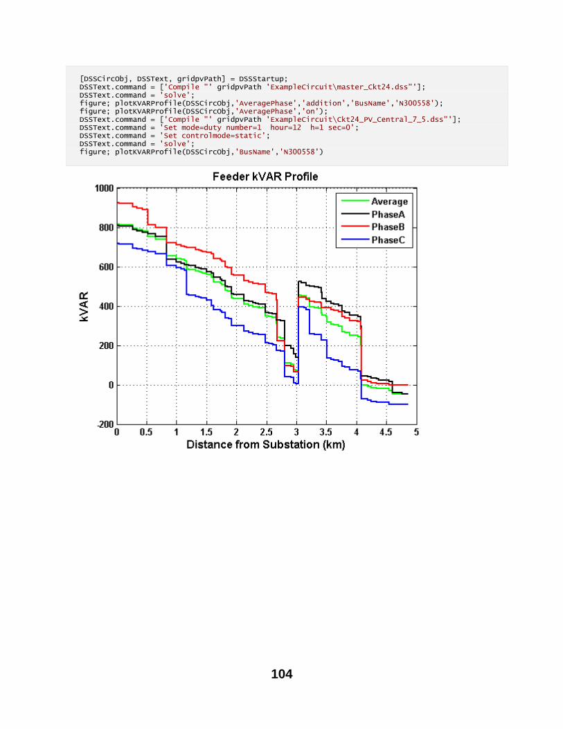
104
[DSSCircObj, DSSText, gridpvPath] = DSSStartup; DSSText.command = ['Compile "' gridpvPath 'ExampleCircuit\master_Ckt24.dss"']; DSSText.command = 'solve'; figure; plotKVARProfile(DSSCircObj,'AveragePhase','addition','BusName','N300558'); figure; plotKVARProfile(DSSCircObj,'AveragePhase','on'); DSSText.command = ['Compile "' gridpvPath 'ExampleCircuit\Ckt24_PV_Central_7_5.dss"']; DSSText.command = 'Set mode=duty number=1 hour=12 h=1 sec=0'; DSSText.command = 'Set controlmode=static'; DSSText.command = 'solve'; figure; plotKVARProfile(DSSCircObj,'BusName','N300558')
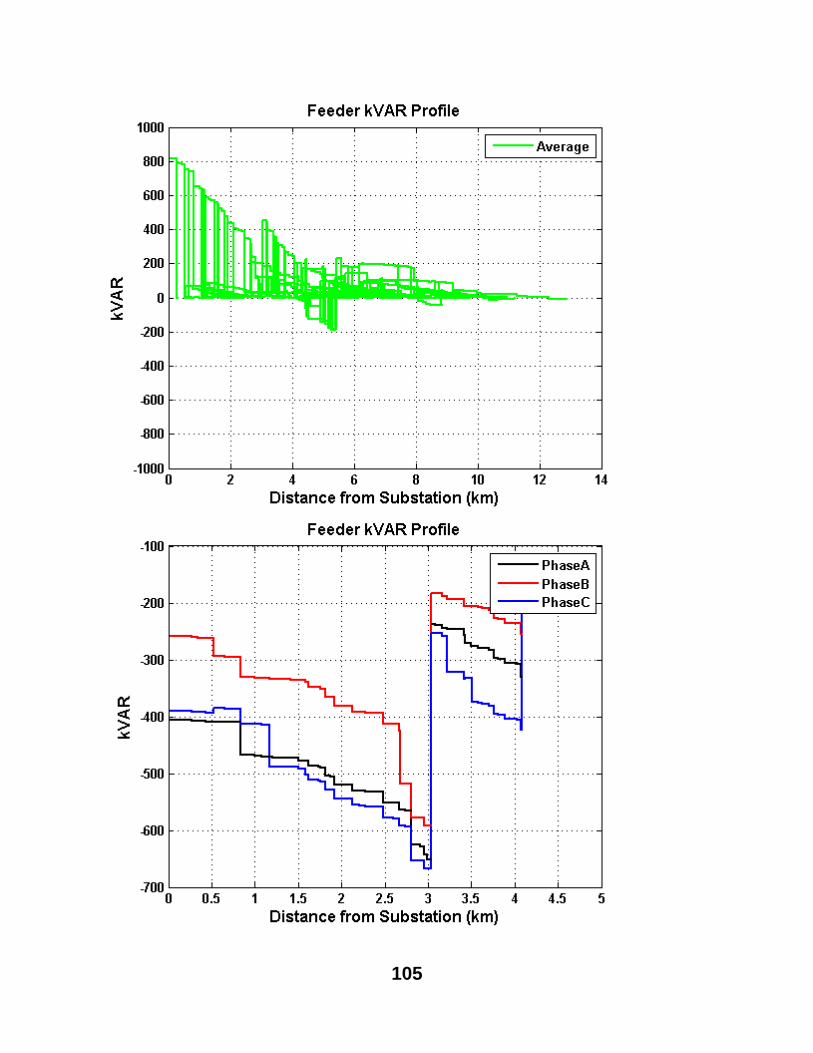
105

106
6.3.5. plotKWProfile
Plots the feeder profile for the kW power flow on the lines
Syntax plotKWProfile(DSSCircObj); plotKWProfile(DSSCircObj, _'PropertyName'_ ,PropertyValue);
Description
Function to plot the feeder profile for the kW power flow on the lines. This is the kW power vs.
distance from the substation graph. Clicking on objects in the figure will display the name of the
object, and right clicking will give a menu for viewing properties of the object.
Inputs
DSSCircObj - link to OpenDSS active circuit and command text (from DSSStartup)
Properties - optional properties as one or more name-value pairs in any order
-- 'Only3Phase' - Property for if only 3-phase power lines should be plotted 'on' | {'off'}
-- 'AveragePhase' - Property for if the average power should be plotted alone or in addition
to the phase plots 'on' | {'off'} | 'addition'
-- 'BusName' - Property for the name of the bus (string) that the kW profile should be plotted
to. Only the direct line between the bus and the substation will be plotted, unless all buses are
selected. {'all'} | busName
-- 'Downstream' - If a BusName is given, all buses in the electrical path to the substation
(upstream) will be plotted, and if this property is on, all buses in the electrical path downstream
of BusName will be plotted too 'on' | {'off'}
-- 'PVMarker' - Property for if the PV PCC should be marked (if it exists) {'on'} | 'off'
-- 'Lines' - Structure of the circuit lines from getLineInfo. If no input is given, the structure is
filled from the most current power flow solution in DSSCircObj COM.
-- 'PV' - Structure of the PV from getPVInfo. If no input is given, the structure is filled from the
most current power flow solution in DSSCircObj COM.
Outputs
none - a figure is displayed with the plot
Notes
For the right-click visualizations, the AllowForms field of DSSCircObj must be set to 1, which is
the default value. Currently, OpenDSS 7.6.3 (the current version as of this writing) does not
allow for setting the AllowForms field back to 1 after setting it to 0.
Example
Example of a feeder kW profile plot
107
[DSSCircObj, DSSText, gridpvPath] = DSSStartup; DSSText.command = ['Compile "' gridpvPath 'ExampleCircuit\master_Ckt24.dss"']; DSSText.command = 'solve'; figure; plotKWProfile(DSSCircObj,'AveragePhase','addition','BusName','N300558'); figure; plotKWProfile(DSSCircObj,'AveragePhase','on'); DSSText.command = ['Compile "' gridpvPath 'ExampleCircuit\Ckt24_PV_Central_7_5.dss"']; DSSText.command = 'Set mode=duty number=1 hour=12 h=1 sec=0'; DSSText.command = 'Set controlmode=static'; DSSText.command = 'solve'; figure; plotKWProfile(DSSCircObj,'BusName','N300558')
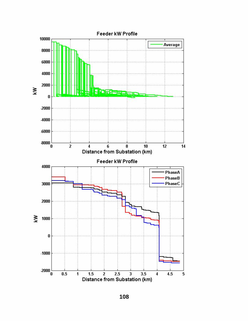
108
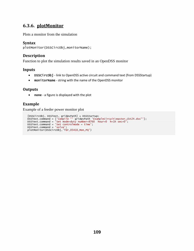
109
6.3.6. plotMonitor
Plots a monitor from the simulation
Syntax plotMonitor(DSSCircObj,monitorName);
Description
Function to plot the simulation results saved in an OpenDSS monitor
Inputs
DSSCircObj - link to OpenDSS active circuit and command text (from DSSStartup)
monitorName - string with the name of the OpenDSS monitor
Outputs
none - a figure is displayed with the plot
Example
Example of a feeder power monitor plot
[DSSCircObj, DSSText, gridpvPath] = DSSStartup; DSSText.command = ['Compile "' gridpvPath 'ExampleCircuit\master_Ckt24.dss"']; DSSText.command = 'Set mode=duty number=8760 hour=0 h=1h sec=0'; DSSText.command = 'Set controlmode = time'; DSSText.command = 'solve'; plotMonitor(DSSCircObj,'fdr_05410_Mon_PQ')
110
111
6.3.7. plotVoltageProfile
Plots the voltage profile for the feeder (spider plot)
Syntax plotVoltageProfile(DSSCircObj); plotVoltageProfile(DSSCircObj, _'PropertyName'_ ,PropertyValue); Handles = plotVoltageProfile(DSSCircObj, _'PropertyName'_ ,PropertyValue);
Description
Function to plot the voltage profile for the feeder. This is the bus voltage vs. distance from the
substation plot. Also called a spider plot. Clicking on objects in the figure will display the name
of the object, and right clicking will give a menu for viewing properties of the object.
Inputs
DSSCircObj - link to OpenDSS active circuit and command text (from DSSStartup)
Properties - optional properties as one or more name-value pairs in any order
-- 'SecondarySystem' - Property for if the secondary system (<600V) should be plotted (if it
exists) {'on'} | 'off'
-- 'Only3Phase' - Property for if only 3-phase power lines should be plotted 'on' | {'off'}
-- 'AveragePhase' - Property for if the average voltage should be plotted alone or in addition
to the phase plots 'on' | {'off'} | 'addition'
-- 'LineToLine' - Property for if the voltage should be line-to-neutral or line-to-line 'on' | {'off'}
-- 'VoltScale' - Property for the y-axis voltage scale {'120'} | 'pu'
-- 'DistanceScale' - Property for the x-axis distance scale {'km'} | 'mi' | 'ft'
-- 'BackgroundShade' - Property for if the range of voltage values should be shaded as an
area 'on' | {'off'}
-- 'BusName' - Property for the name of the bus (string) that the voltage profile should be
plotted to. Only the direct line between the bus and the substation will be plotted, unless all
buses are selected. {'all'} | busName
-- 'Downstream' - If a BusName is given, all buses in the electrical path to the substation
(upstream) will be plotted, and if this property is on, all buses in the electrical path downstream
of BusName will be plotted too 'on' | {'off'}
-- 'PVMarker' - Property for if the PV PCC should be marked {'on'} | 'off'
-- 'CapacitorMarker' - Property for if capacitors should be marked 'on' | {'off'}
-- 'Lines' - Structure of the circuit lines from getLineInfo. If no input is given, the structure is
filled from the most current power flow solution in DSSCircObj COM.
-- 'Transformers' - Structure of the circuit transformers from getTransformerInfo. If no
input is given, the structure is filled from the most current power flow solution in DSSCircObj
COM.
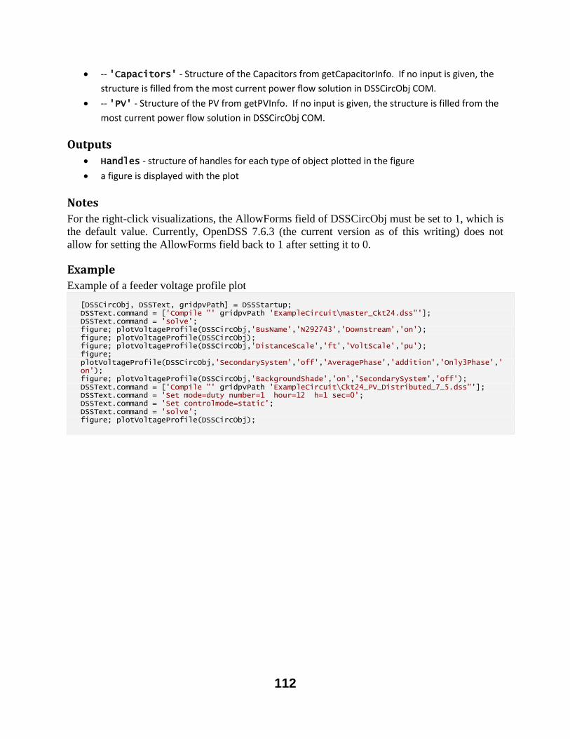
112
-- 'Capacitors' - Structure of the Capacitors from getCapacitorInfo. If no input is given, the
structure is filled from the most current power flow solution in DSSCircObj COM.
-- 'PV' - Structure of the PV from getPVInfo. If no input is given, the structure is filled from the
most current power flow solution in DSSCircObj COM.
Outputs
Handles - structure of handles for each type of object plotted in the figure
a figure is displayed with the plot
Notes
For the right-click visualizations, the AllowForms field of DSSCircObj must be set to 1, which is
the default value. Currently, OpenDSS 7.6.3 (the current version as of this writing) does not
allow for setting the AllowForms field back to 1 after setting it to 0.
Example
Example of a feeder voltage profile plot
[DSSCircObj, DSSText, gridpvPath] = DSSStartup; DSSText.command = ['Compile "' gridpvPath 'ExampleCircuit\master_Ckt24.dss"']; DSSText.command = 'solve'; figure; plotVoltageProfile(DSSCircObj,'BusName','N292743','Downstream','on'); figure; plotVoltageProfile(DSSCircObj); figure; plotVoltageProfile(DSSCircObj,'DistanceScale','ft','VoltScale','pu'); figure; plotVoltageProfile(DSSCircObj,'SecondarySystem','off','AveragePhase','addition','Only3Phase','on'); figure; plotVoltageProfile(DSSCircObj,'BackgroundShade','on','SecondarySystem','off'); DSSText.command = ['Compile "' gridpvPath 'ExampleCircuit\Ckt24_PV_Distributed_7_5.dss"']; DSSText.command = 'Set mode=duty number=1 hour=12 h=1 sec=0'; DSSText.command = 'Set controlmode=static'; DSSText.command = 'solve'; figure; plotVoltageProfile(DSSCircObj);
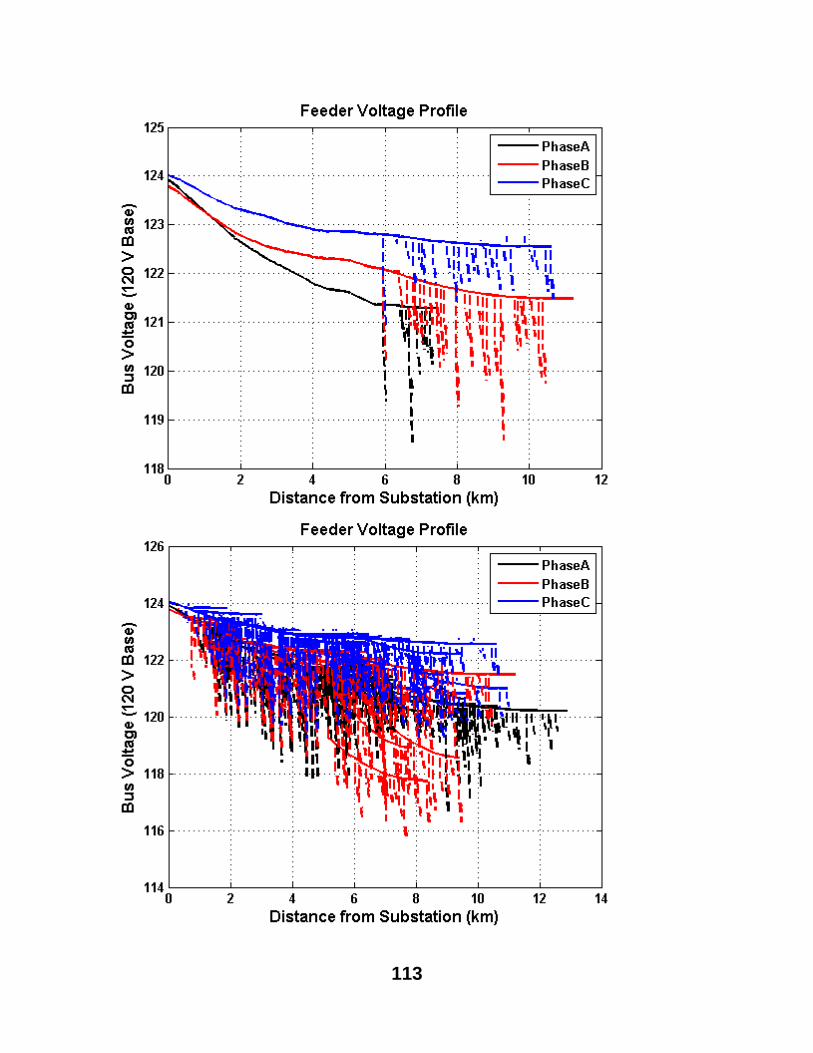
113
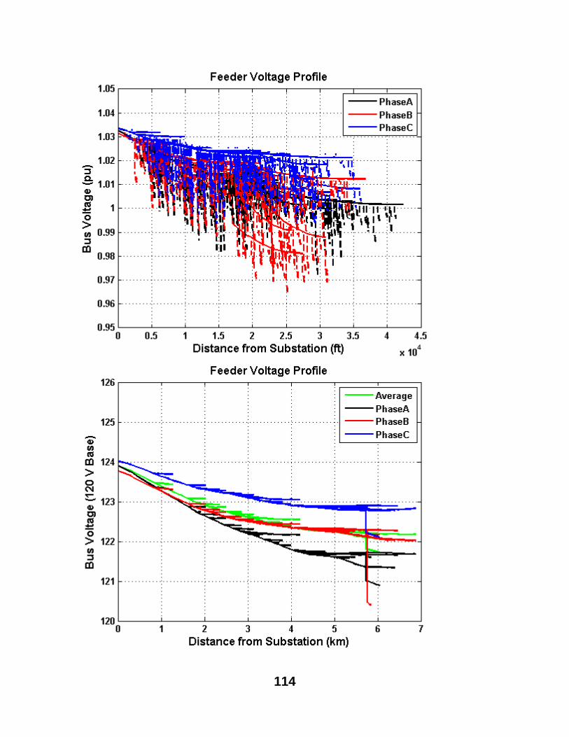
114
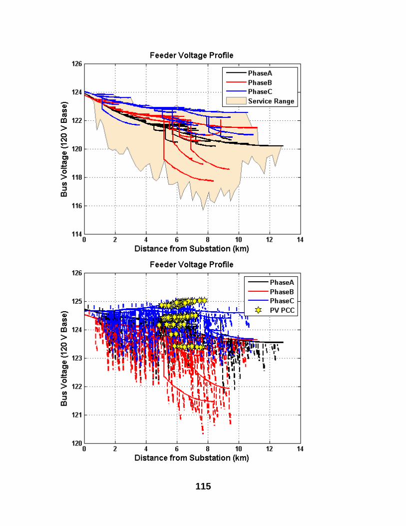
115

116
6.4. GEOGRAPHIC MAPPING FUNCTIONS
If the OpenDSS feeder has geographical information, this can be used to map the feeder to the
real world. The OpenDSS feeder coordinates are generally located in a file called
“Buscoords.dss” and links each bus to an X and Y coordinate. This information comes from the
utility’s coordinate system, which can be UTM, a state coordinate system, or their own
coordinates. If the conversion from the utility coordinate system is unknown, the
createCircuitCoordConversion function tool can be used to visually match the feeder layout to
satellite images.
With a known coordinate system, certain GIS or map plotting features are available in the
toolbox to visualize the location of the distribution system power lines. Google Maps is used to
display streets, location names, and satellite images. The API for Google Maps allows
MATLAB to interact and download maps with location specific data, including elevation [15].
The figure displays an example distribution system demonstrating the GIS functionality [9].
Function List
initCoordConversion - Function to initialize the coordinate conversion process
createCircuitCoordConversion - Function to create conversion of circuit coordinates to GPS coordinates
createCircuitCoordConversionUTM - Function to create conversion of circuit coordinates in UTM to GPS coordinates
plotGoogleMap - Plots a Google map on the current axes using the Google Static Maps API
117
6.4.1. initCoordConversion
Function to initialize the coordinate conversion process
Syntax initCoordConversion();
Description
Function to allow the user to pick between coordinate conversion methods: manual creation or
UTM conversion.
Inputs
None
Outputs
None
Example
initCoordConversion();
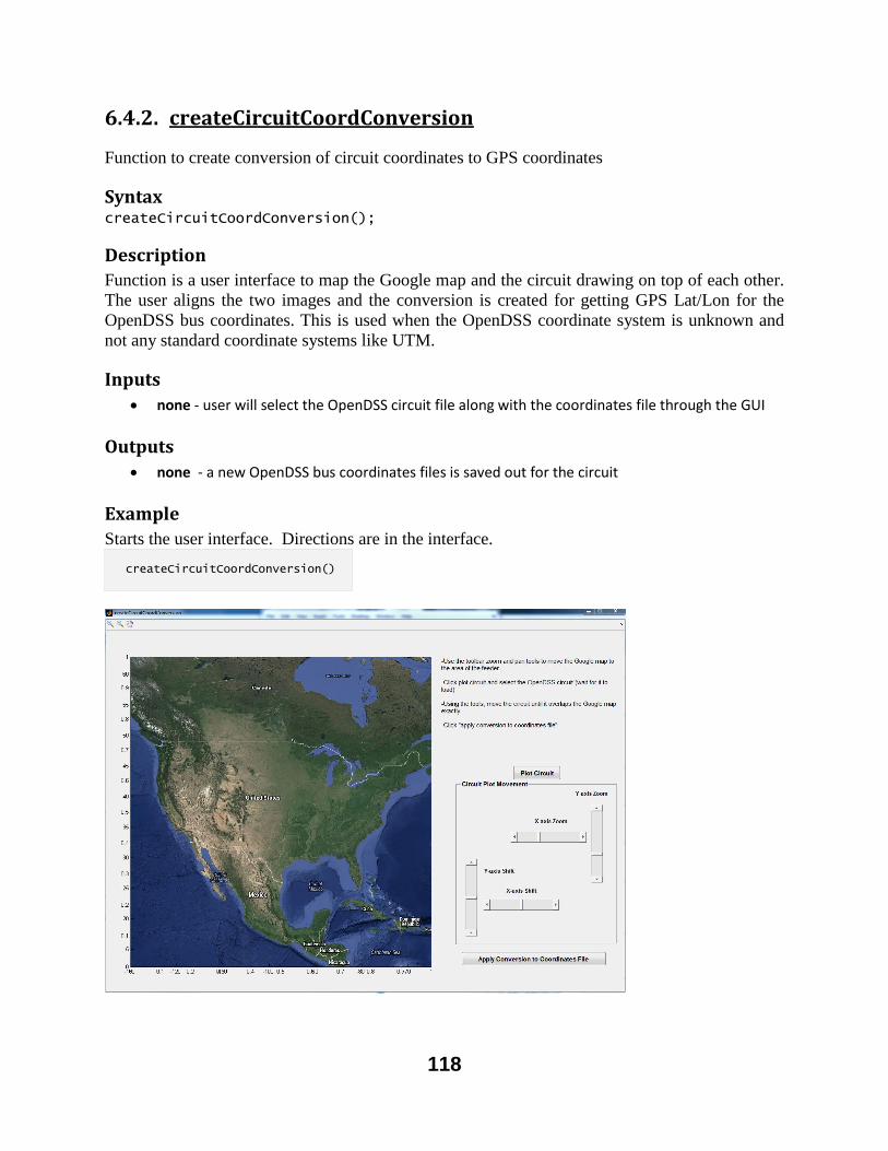
118
6.4.2. createCircuitCoordConversion
Function to create conversion of circuit coordinates to GPS coordinates
Syntax createCircuitCoordConversion();
Description
Function is a user interface to map the Google map and the circuit drawing on top of each other.
The user aligns the two images and the conversion is created for getting GPS Lat/Lon for the
OpenDSS bus coordinates. This is used when the OpenDSS coordinate system is unknown and
not any standard coordinate systems like UTM.
Inputs
none - user will select the OpenDSS circuit file along with the coordinates file through the GUI
Outputs
none - a new OpenDSS bus coordinates files is saved out for the circuit
Example
Starts the user interface. Directions are in the interface.
createCircuitCoordConversion()

119
6.4.3. createCircuitCoordConversionUTM
Function to create conversion of circuit coordinates in UTM to GPS coordinates
Syntax createCircuitCoordConversionUTM();
Description
Function is a user interface that allows the user to select the UTM zone the circuit coordinates
are currently in. The conversion is created for getting GPS Lat/Lon for the OpenDSS bus
coordinates and the new Lat/Lon OpenDSS buscoords are saved.
Inputs
none
Outputs
none - a Circuit Conversion file is saved for any future plotting
Example
Starts the user interface. Directions are in the interface.
createCircuitCoordConversionUTM();
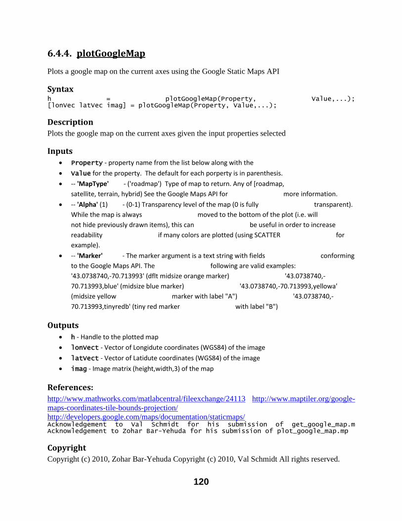
120
6.4.4. plotGoogleMap
Plots a google map on the current axes using the Google Static Maps API
Syntax h = plotGoogleMap(Property, Value,...); [lonVec latVec imag] = plotGoogleMap(Property, Value,...);
Description
Plots the google map on the current axes given the input properties selected
Inputs
Property - property name from the list below along with the
Value for the property. The default for each porperty is in parenthesis.
-- 'MapType' - ('roadmap') Type of map to return. Any of [roadmap,
satellite, terrain, hybrid) See the Google Maps API for more information.
-- 'Alpha' (1) - (0-1) Transparency level of the map (0 is fully transparent).
While the map is always moved to the bottom of the plot (i.e. will
not hide previously drawn items), this can be useful in order to increase
readability if many colors are plotted (using SCATTER for
example).
-- 'Marker' - The marker argument is a text string with fields conforming
to the Google Maps API. The following are valid examples:
'43.0738740,-70.713993' (dflt midsize orange marker) '43.0738740,-
70.713993,blue' (midsize blue marker) '43.0738740,-70.713993,yellowa'
(midsize yellow marker with label "A") '43.0738740,-
70.713993,tinyredb' (tiny red marker with label "B")
Outputs
h - Handle to the plotted map
lonVect - Vector of Longidute coordinates (WGS84) of the image
latVect - Vector of Latidute coordinates (WGS84) of the image
imag - Image matrix (height,width,3) of the map
References:
http://www.mathworks.com/matlabcentral/fileexchange/24113 http://www.maptiler.org/google-
maps-coordinates-tile-bounds-projection/
http://developers.google.com/maps/documentation/staticmaps/ Acknowledgement to Val Schmidt for his submission of get_google_map.m Acknowledgement to Zohar Bar-Yehuda for his submission of plot_google_map.mp
Copyright
Copyright (c) 2010, Zohar Bar-Yehuda Copyright (c) 2010, Val Schmidt All rights reserved.

121
Redistribution and use in source and binary forms, with or without modification, are permitted
provided that the following conditions are met: * Redistributions of source code must retain the above copyright notice, this list of conditions and the following disclaimer. * Redistributions in binary form must reproduce the above copyright notice, this list of conditions and the following disclaimer in the documentation and/or other materials provided with the distribution THIS SOFTWARE IS PROVIDED BY THE COPYRIGHT HOLDERS AND
CONTRIBUTORS "AS IS" AND ANY EXPRESS OR IMPLIED WARRANTIES,
INCLUDING, BUT NOT LIMITED TO, THE IMPLIED WARRANTIES OF
MERCHANTABILITY AND FITNESS FOR A PARTICULAR PURPOSE ARE
DISCLAIMED. IN NO EVENT SHALL THE COPYRIGHT OWNER OR CONTRIBUTORS
BE LIABLE FOR ANY DIRECT, INDIRECT, INCIDENTAL, SPECIAL, EXEMPLARY, OR
CONSEQUENTIAL DAMAGES (INCLUDING, BUT NOT LIMITED TO, PROCUREMENT
OF SUBSTITUTE GOODS OR SERVICES; LOSS OF USE, DATA, OR PROFITS; OR
BUSINESS INTERRUPTION) HOWEVER CAUSED AND ON ANY THEORY OF
LIABILITY, WHETHER IN CONTRACT, STRICT LIABILITY, OR TORT (INCLUDING
NEGLIGENCE OR OTHERWISE) ARISING IN ANY WAY OUT OF THE USE OF THIS
SOFTWARE, EVEN IF ADVISED OF THE POSSIBILITY OF SUCH DAMAGE.
Example
Plot a map showing some capitals in Europe:
lat = [48.8708 51.5188 41.9260 40.4312 52.523 37.982]; lon = [2.4131 -0.1300 12.4951 -3.6788 13.415 23.715]; plot(lon,lat,'.r','MarkerSize',20) plotGoogleMap
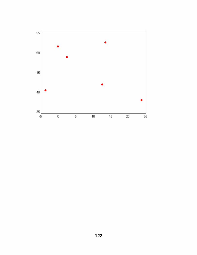
122
123
6.5. SOLAR MODELING FUNCTIONS
Simulating the impact of solar on the distribution system requires an accurate timeseries of PV
plant power output. The OpenDSS model is used to model the feeder and the loads, but
MATLAB is used to setup the PV plant model. The process of modeling solar plant output
begins with measured irradiance data. Generally, a specific day or time of year is used for
simulation. The IneichenClearSkyModel function can be used to generate a Global Horizontal
Irradiance time-series for a clear day for any location and dates to simulate the maximum output
from PV on the system each day [16]. Another method would be to identify a highly variable
day from measured irradiance data to simulate the impact of PV variability [17].
To simulate a PV plant from irradiance data, the PV plant information is setup using the user
interface in the placePVplant function. The interface allows the user to draw the location of a
PV plant directly on the Google map and feeder layout. The drawn PV plant is used for
smoothing the plant variability using the Wavelet Variability Model (WVM) [18-20]. There are
also several options for controlling the power factor of the PV output, such as a power factor
schedule, power factor function of output, and volt/var control [14, 21, 22]. The function
createPVscenarioFiles will run the WVM model and create the OpenDSS solar scenario case
files with the correct loadshape for solar output and PV generators placed on the correct bus
locations.
Function List
placePVplant - Draw PV on the circuit diagram and save plant info for WVM input
createPVscenarioFiles - Runs the WVM model and puts out the OpenDSS PV scenario files
distributePV - Allocates PV based off of the load transformer size (kva)
findMaxPenetrationTime - Finds the max penetration time
IneichenClearSkyModel - Generates the clear sky irradiance using Ineichen and Perez model
makePFoutputFunction - GUI for creating power factor as a function of PV power output
makePFprofile - Creates varying Power Factor profile by schedule or PV output
makePFschedule - GUI for creating a power factor daily schedule
makeVVCcurve - GUI for setting up the OpenDSS VVControl function parameters
pvl_WVM - WVM Wavelet Variability Model
124
6.5.1. placePVplant
Draw PV on the circuit diagram and save plant info for WVM input
Syntax placePVplant()
Description
This function is a user interface where the PV plant can be drawn on the circuit diagram. The
user will setup all the PV plant info and save it to a file for running WVM.
Inputs
none
Outputs
none saves a *.mat file with the structure plantinfo for input to WVM
Example
Showing the user interface:
placePVplant() %
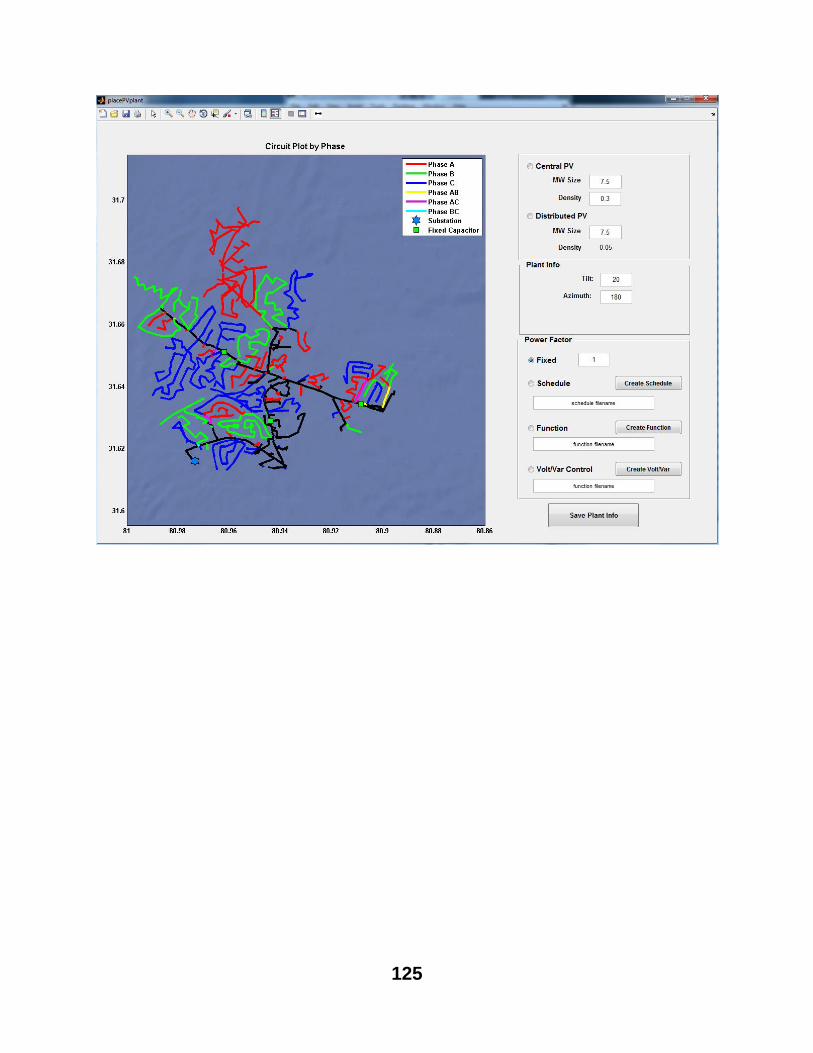
125
126
6.5.2. createPVscenarioFiles
Runs the WVM model and puts out the OpenDSS PV scenario files
Syntax index = createPVscenarioFiles(plantInfoFile,irradianceFile,A_value,circuitFile); index = createPVscenarioFiles();
Description
Function to load in the inputs to the WVM (plant info and irradiance sensor info), run WVM,
create the loadshape file, and the solar scenario OpenDSS file.
Inputs
plantInfoFile - optional input with the link to the MAT file with the require PV plant
information structure for WVM (see WVM.m and placePVplant.m)
irradianceFile - optional input with the link to the MAT file with the require irradiance
sensor information structure for WVM (see pvl_WVM.m)
cloud_speed - optional input with a single value of the daily cloud speed
circuitFile - optional input with the link to the file with the OpenDSS circuit
Outputs
none - outputs both a .txt loadshape file and a .dss solar scenario OpenDSS file
Example
Example run of createPVscenarioFiles
createPVscenarioFiles('./ExampleCircuit/Ckt24_PV_Central_7_5.mat','./Subfunctions/WVM_subfunctions/Livermore_irr_sensor.mat',10,'.\ExampleCircuit\master_ckt24.dss'); %
127
6.5.3. distributePV
Allocates PV based off of the load transformer size (kva)
Syntax distributePV(totalPVSize,area)
Description
Allocates distributed PV spread out around a designated area. PV is placed at each transformer
in the area based off of the load transformer size (kva). The user is asked to select the OpenDSS
circuit through the GUI.
Inputs
totalPVSize - total size of the distributed PV system in kW
area - matrix of vertices defining the area to distribute the PV inside, 1 row per vertex with [X,Y]
Outputs
text file allocatedPV.txt with the OpenDSS text for PV systems as generators
Example
Distributes the total PV size around the given area.
area = [1.1732e7 3.708e6; 1.1732e6 3.728e6; 1.1748e7 3.708e6; 1.1748e7 3.728e6]; totalPVSize = 2e3; distributePV(totalPVSize,area);
128
6.5.4. findMaxPenetrationTime
Finds the max penetration time
Syntax index = findMaxPenetrationTime(loadFile,pvFile); index = findMaxPenetrationTime();
Description
Function to calculate when the max penetration (PV output / load) time occurs. User inputs the
load file and PV output profile, max time is calculated.
Inputs
loadFile - optional input with the link to the file with the load data
pvFile - optional input with the link to the file with the PV output data
Outputs
index - the index in the array with the maximum penetration
Example
Finds the maximum penetration time for sample files
index = 39125
index = findMaxPenetrationTime('ExampleCircuit\LS_ThreePhase.txt','ExampleCircuit\PVloadshape_7_5MW_Central.txt')
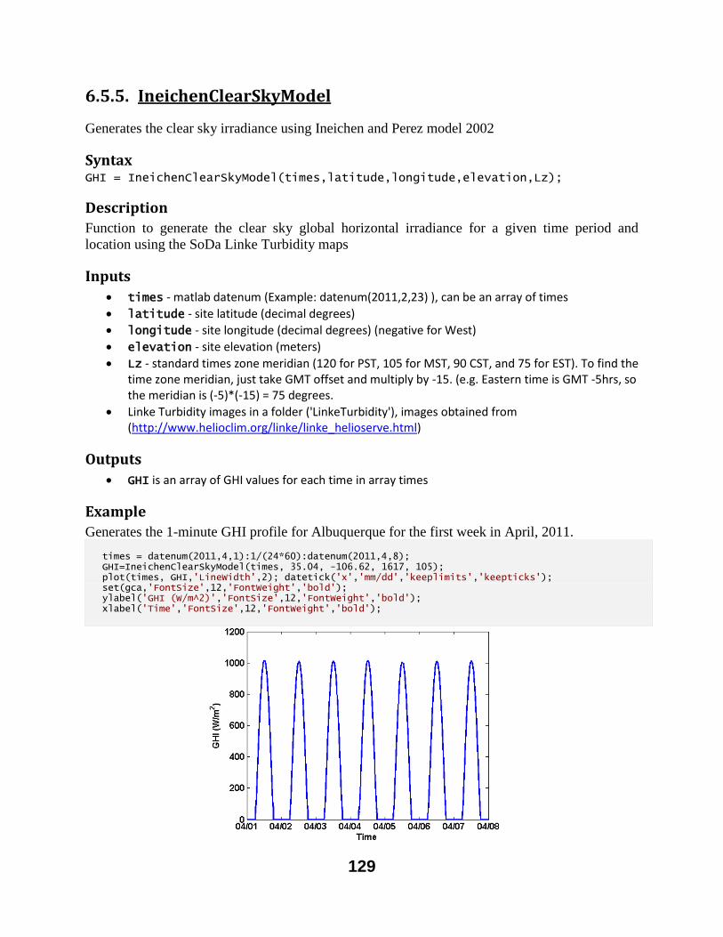
129
6.5.5. IneichenClearSkyModel
Generates the clear sky irradiance using Ineichen and Perez model 2002
Syntax GHI = IneichenClearSkyModel(times,latitude,longitude,elevation,Lz);
Description
Function to generate the clear sky global horizontal irradiance for a given time period and
location using the SoDa Linke Turbidity maps
Inputs
times - matlab datenum (Example: datenum(2011,2,23) ), can be an array of times
latitude - site latitude (decimal degrees)
longitude - site longitude (decimal degrees) (negative for West)
elevation - site elevation (meters)
Lz - standard times zone meridian (120 for PST, 105 for MST, 90 CST, and 75 for EST). To find the time zone meridian, just take GMT offset and multiply by -15. (e.g. Eastern time is GMT -5hrs, so the meridian is (-5)*(-15) = 75 degrees.
Linke Turbidity images in a folder ('LinkeTurbidity'), images obtained from (http://www.helioclim.org/linke/linke_helioserve.html)
Outputs
GHI is an array of GHI values for each time in array times
Example
Generates the 1-minute GHI profile for Albuquerque for the first week in April, 2011.
times = datenum(2011,4,1):1/(24*60):datenum(2011,4,8); GHI=IneichenClearSkyModel(times, 35.04, -106.62, 1617, 105); plot(times, GHI,'LineWidth',2); datetick('x','mm/dd','keeplimits','keepticks'); set(gca,'FontSize',12,'FontWeight','bold'); ylabel('GHI (W/m^2)','FontSize',12,'FontWeight','bold'); xlabel('Time','FontSize',12,'FontWeight','bold');
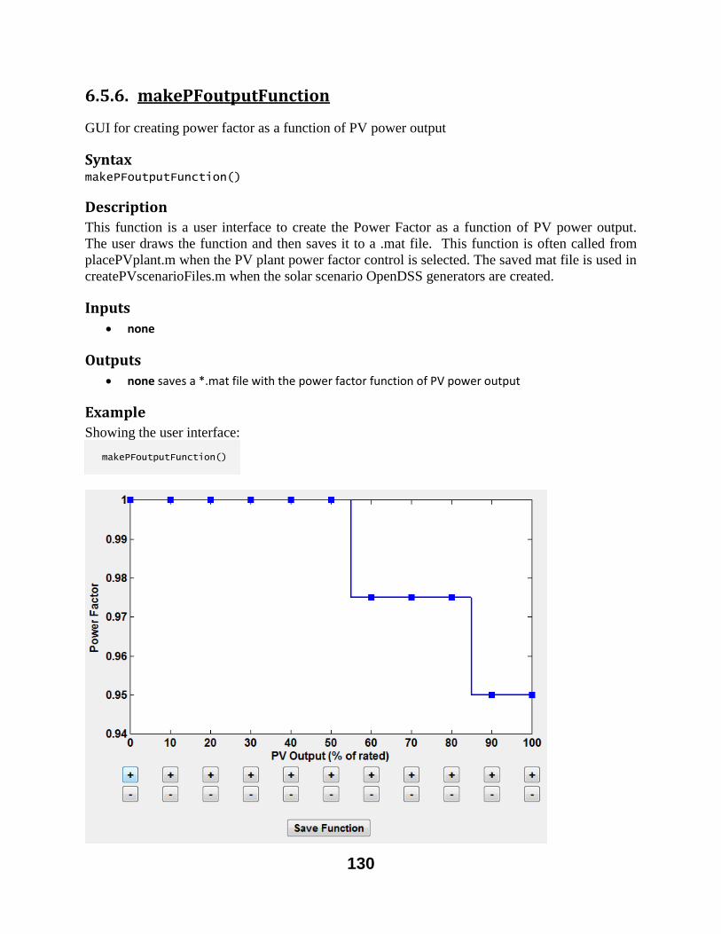
130
6.5.6. makePFoutputFunction
GUI for creating power factor as a function of PV power output
Syntax makePFoutputFunction()
Description
This function is a user interface to create the Power Factor as a function of PV power output.
The user draws the function and then saves it to a .mat file. This function is often called from
placePVplant.m when the PV plant power factor control is selected. The saved mat file is used in
createPVscenarioFiles.m when the solar scenario OpenDSS generators are created.
Inputs
none
Outputs
none saves a *.mat file with the power factor function of PV power output
Example
Showing the user interface:
makePFoutputFunction()
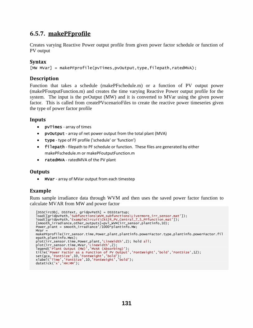
131
6.5.7. makePFprofile
Creates varying Reactive Power output profile from given power factor schedule or function of
PV output
Syntax [MW MVar] = makePFprofile(pvTimes,pvOutput,type,filepath,ratedMVA);
Description
Function that takes a schedule (makePFschedule.m) or a function of PV output power
(makePFoutputFunction.m) and creates the time varying Reactive Power output profile for the
system. The input is the pvOutput (MW) and it is converted to MVar using the given power
factor. This is called from createPVscenarioFiles to create the reactive power timeseries given
the type of power factor profile
Inputs
pvTimes - array of times
pvOutput - array of net power output from the total plant (MVA)
type - type of PF profile ('schedule' or 'function')
filepath - filepath to PF schedule or function. These files are generated by either
makePFschedule.m or makePFoutputFunction.m
ratedMVA - ratedMVA of the PV plant
Outputs
MVar - array of MVar output from each timestep
Example
Runs sample irradiance data through WVM and then uses the saved power factor function to
calculate MVAR from MW and power factor
[DSSCircObj, DSSText, gridpvPath] = DSSStartup; load([gridpvPath,'Subfunctions\WVM_subfunctions\Livermore_irr_sensor.mat']); load([gridpvPath,'ExampleCircuit\Ckt24_PV_Central_7_5_PFfunction.mat']); [smooth_irradiance,other_outputs]=pvl_WVM(irr_sensor,plantinfo,10); Power_plant = smooth_irradiance'/1000*plantinfo.MW; MVar = makePFprofile(irr_sensor.time,Power_plant,plantinfo.powerFactor.type,plantinfo.powerFactor.filepath,plantinfo.MWs); plot(irr_sensor.time,Power_plant,'LineWidth',2); hold all; plot(irr_sensor.time,MVar,'LineWidth',2); legend('Plant Output (MW)','MVAR (Absorbing)'); title('Power Factor as a Function of PV Output','FontWeight','bold','FontSize',12); set(gca,'FontSize',10,'FontWeight','bold'); xlabel('Time','FontSize',10,'FontWeight','bold'); datetick('x','HH:MM');
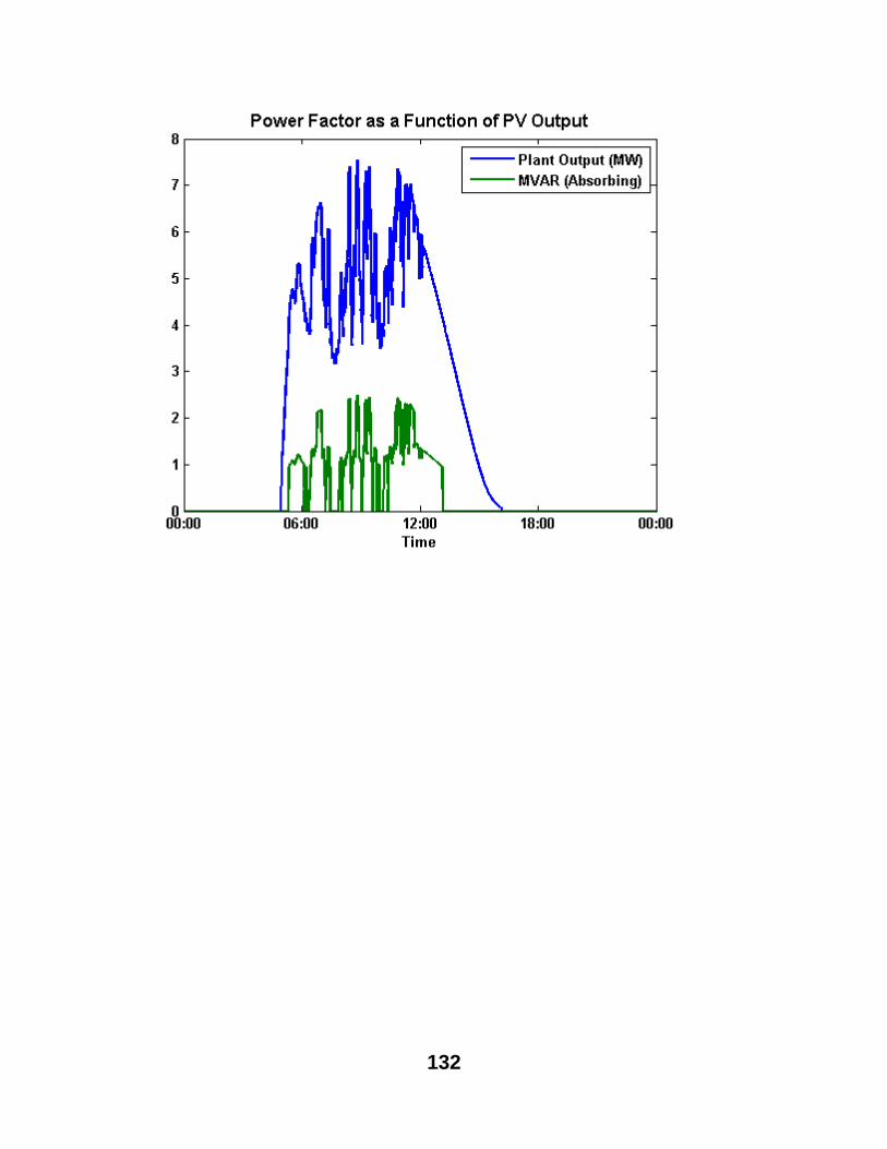
132
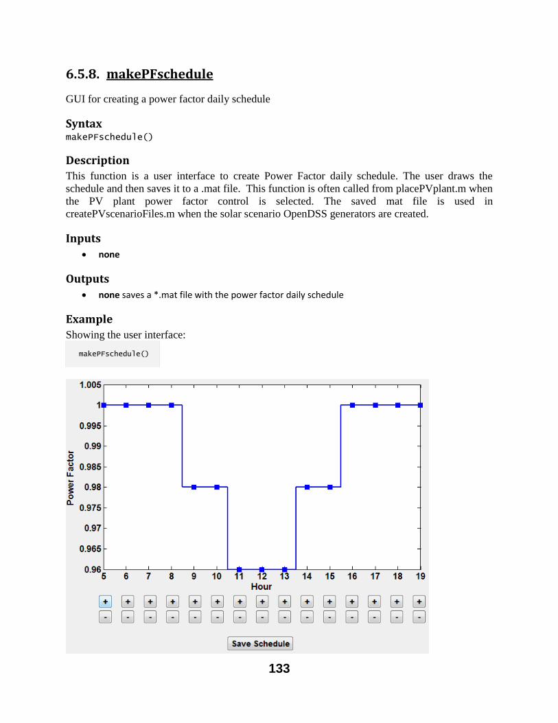
133
6.5.8. makePFschedule
GUI for creating a power factor daily schedule
Syntax makePFschedule()
Description
This function is a user interface to create Power Factor daily schedule. The user draws the
schedule and then saves it to a .mat file. This function is often called from placePVplant.m when
the PV plant power factor control is selected. The saved mat file is used in
createPVscenarioFiles.m when the solar scenario OpenDSS generators are created.
Inputs
none
Outputs
none saves a *.mat file with the power factor daily schedule
Example
Showing the user interface:
makePFschedule()
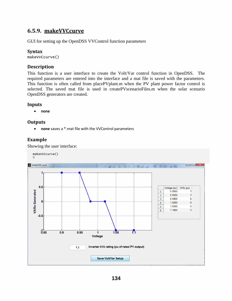
134
6.5.9. makeVVCcurve
GUI for setting up the OpenDSS VVControl function parameters
Syntax makeVVCcurve()
Description
This function is a user interface to create the Volt/Var control function in OpenDSS. The
required parameters are entered into the interface and a mat file is saved with the parameters.
This function is often called from placePVplant.m when the PV plant power factor control is
selected. The saved mat file is used in createPVscenarioFiles.m when the solar scenario
OpenDSS generators are created.
Inputs
none
Outputs
none saves a *.mat file with the VVControl parameters
Example
Showing the user interface:
makeVVCcurve() %

135
6.5.10. pvl_WVM
Wavelet Variability Model
Syntax:
smooth_irradiance = pvl_wvm(irr_sensor,plantinfo,cloud_speed);
Description
Computes the spatially-smoothed irradiance to convert a point irradiance sensor to represent a
large PV array with decreased ramps. The method uses the wavelet variability model at different
time scales to provide all cooresponding smoothing.
Inputs
irr_sensor is a struct with variables:
irr_sensor.irr: the irradiance measurement
irr_sensor.time: the time stamps (Matlab time vector) for irr_sensor.irr
irr_sensor.Lat: latitude of the sensor
irr_sensor.Lon: longitude of the sensor
irr_sensor.alt: altitude of the sensor
irr_sensor.tilt: tilt angle of the sensor, 0 = flat (e.g., GHI)
irr_sensor.azimuth: azimuth angle of the sensor, 180 = due south
irr.sensor.clear_sky_irradiance: (optional input) manually enter the clear-sky irradiance (e.g.,
for an irradiance sensor on a tracking system)
irr_sensor.UTCoffset=UTC offset
plantinfo is a struct describing the plant to simulate with variables:
plantinfo.tilt: tilt angle of plant modules
plantinfo.azimuth: azimuth angle of plant modules
plantinfo.clear_sky_irrPOA: (optional input) manually enter the clear-sky irradiance in the
module POA (e.g., for tracking systems)
plantinfo.type: 'square','polygon',' or 'discrete' 'square' square PV plant with specified
number of MWs and PV density 'polygon' custom PV plant shape (define vetiticies in lat/lon)
'discrete' simulate only certain points (e.g., to replicate output of multiple point sensors)
plantinfo.MW: = MW of PV installed (not necessary for 'discrete' type)
plantinfo.PVdensity: = W PV installed per m2 in plant area (e.g., 41 W/m2 is 1MW per 6 acres)
(not necessary for 'discrete' type)
plantinfo.Lat: (only needed for type 'polygon' or 'discrete') latitude of polygon verticies or
discrete points
plantinfo.Lon: (only needed for type 'polygon' or 'discrete') longitude of polygon verticies or
discrete points
cloud_speed is a single value of the daily cloud speed
Outputs
136
|smooth_irradiance| is the WVM smoothed irradiance representing the average irradiance over
the plant footprint. It maintains the time stamps of the input irradiance (irr_sensor.time).
BSD License:
Copyright (c) 2012, The Regents of the University of California All rights reserved.
Redistribution and use in source and binary forms, with or without modification, are permitted
provided that the following conditions are met: Redistributions of source code must retain the
above copyright notice, this list of conditions and the following disclaimer. Redistributions in
binary form must reproduce the above copyright notice, this list of conditions and the following
disclaimer in the documentation and/or other materials provided with the distribution. Neither
the name The Regents of the University of California, the names of its campuses nor any
abbreviation thereof, nor the names of the contributors may be used to endorse or promote
products derived from this software without specific prior written permission. THIS
SOFTWARE IS PROVIDED BY THE COPYRIGHT HOLDERS AND CONTRIBUTORS "AS
IS" AND ANY EXPRESS OR IMPLIED WARRANTIES, INCLUDING, BUT NOT LIMITED
TO, THE IMPLIED WARRANTIES OF MERCHANTABILITY AND FITNESS FOR A
PARTICULAR PURPOSE ARE DISCLAIMED. IN NO EVENT SHALL THE COPYRIGHT
HOLDER OR CONTRIBUTORS BE LIABLE FOR ANY DIRECT, INDIRECT,
INCIDENTAL, SPECIAL, EXEMPLARY, OR CONSEQUENTIAL DAMAGES
(INCLUDING, BUT NOT LIMITED TO, PROCUREMENT OF SUBSTITUTE GOODS OR
SERVICES; LOSS OF USE, DATA, OR PROFITS; OR BUSINESS INTERRUPTION)
HOWEVER CAUSED AND ON ANY THEORY OF LIABILITY, WHETHER IN
CONTRACT, STRICT LIABILITY, OR TORT (INCLUDING NEGLIGENCE OR
OTHERWISE) ARISING IN ANY WAY OUT OF THE USE OF THIS SOFTWARE, EVEN IF
ADVISED OF THE POSSIBILITY OF SUCH DAMAGE.
Example
This example uses May 18th, 2014 irradiance data collected at Sandia National Laboratories in
Livermore, CA to demonstrate use of the wavelet variability model (WVM).
Livermore=load('.\WVM_subfunctions\Livermore_Sample_GHI.mat'); irr_sensor.irr=Livermore.GHI; %measured irradiance irr_sensor.time=Livermore.dt; %timestamps irr_sensor.Lat=37.676208; %sensor latitude irr_sensor.Lon=-121.703118; %sensor longitude irr_sensor.alt=200; %sensor altitude (in meters) irr_sensor.tilt=0; %tilt = 0 for GHI sensor irr_sensor.azimuth=180; %180 = due south irr_sensor.UTCoffset=-8; %sensor UTC offset plantinfo.tilt=37; %assume modules tilted 37 degrees (approximately latitude tilt) plantinfo.azimuth=180; %assume modules facing south plantinfo.type='square'; %assume a square-shaped PV plant plantinfo.MW=30; %assume a 30MW plant plantinfo.PVdensity=41; %41 W/m2 = 1MW per 6 acres, which is a standard rule of thumb cloud_speed=10; %assume cloud speed of 10 m/s [smooth_irradiance,other_outputs]=pvl_WVM(irr_sensor,plantinfo,cloud_speed); plot(irr_sensor.time,irr_sensor.irr,'b',irr_sensor.time,smooth_irradiance,'r'); %Zoomed in plot comparing the measured GHI to the WVM output of smoothed POA irradiance. legend('measured GHI','WVM smoothed POA'); set(gca,'xtick',floor(nanmean(irr_sensor.time)):1/(24*12):ceil(nanmean(irr_sensor.time))); datetick('x','HH:MM','keepticks','keeplimits'); xlabel('time of day [HH:MM]');ylabel('Irradiance [W m^{-2}]'); xlim([floor(nanmean(irr_sensor.time))+10.75/24 floor(nanmean(irr_sensor.time))+11.25/24]); title(datestr(nanmean(irr_sensor.time),'mmm-dd-yyyy'));
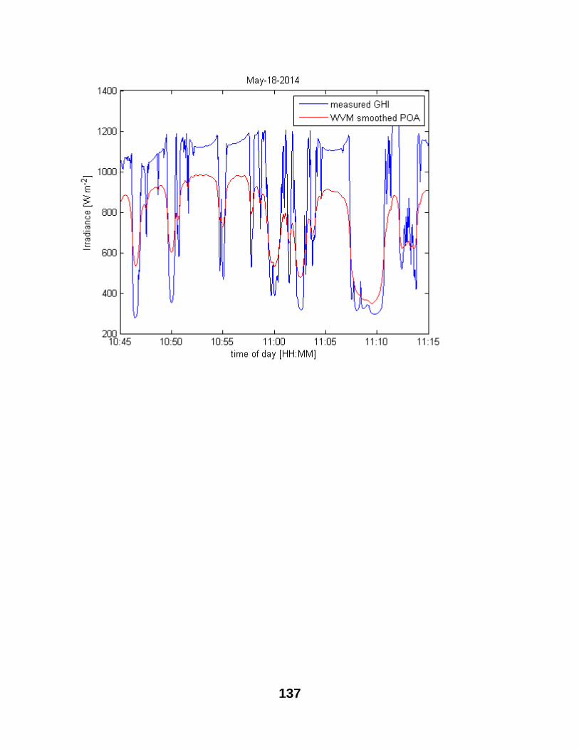
137

139
6.6. EXAMPLE SIMULATIONS
These functions serve as examples for running simulations and analysis of solar on the
distribution system in OpenDSS. Once the feeder is setup in OpenDSS and the solar scenarios
are created, these functions can loop through the different predefined cases and perform analysis
during the simulations. As examples, these functions can be modified to perform any other
research analysis in the same framework with snapshot analyses or timeseries analyses.
Function List
examplePeakTimeAnalysis - Runs simulation during peak penetration time and generates plots
exampleTimeseriesAnalyses - Timeseries analysis and plots monitor values from the simulation
exampleVoltageAnalysis - Example analysis of maximum and minimum feeder voltages through time
140
6.6.1. examplePeakTimeAnalysis
Runs simulation during peak penetration time and generates plots
Syntax examplePeakTimeAnalysis(basecaseFile,solarScenarioFiles); examplePeakTimeAnalysis();
Description
Function to calculate when the max penetration (PV output / load) time occurs. A snapshot
analysis is performed at this peak time, with both a voltage contour plot and voltage profile plot
being generated.
Inputs
basecaseFile - optional input with the link to the OpenDSS file with the circuit.
solarScenarioFiles - optional input with a cell array of links to the OpenDSS files with the
solar scenarios to run
Outputs
none - generates 2 figures for each analysis scenario and saves them
Example
Runs the basecase circuit and the distributed solar case
examplePeakTimeAnalysis('ExampleCircuit\master_ckt24.dss',{'ExampleCircuit\Ckt24_PV_Distributed_7_5.dss'})
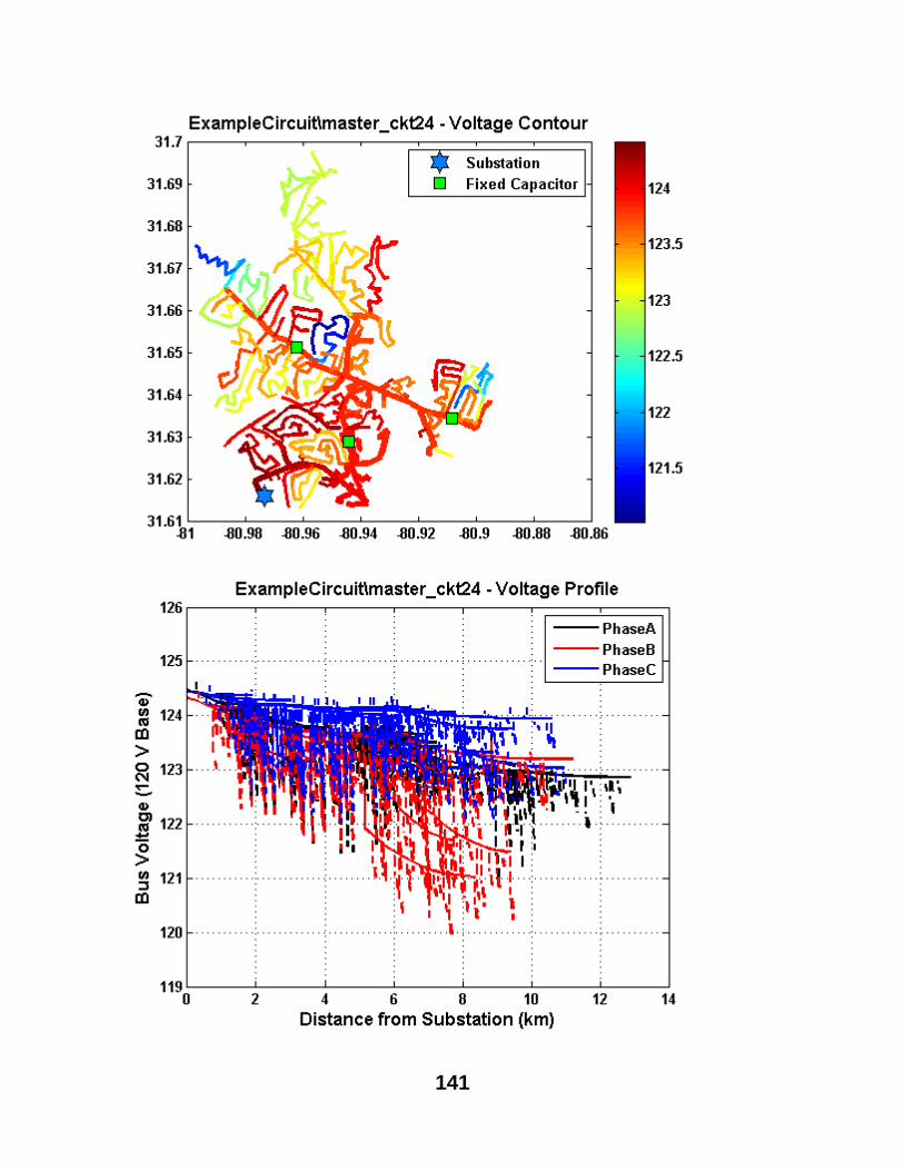
141
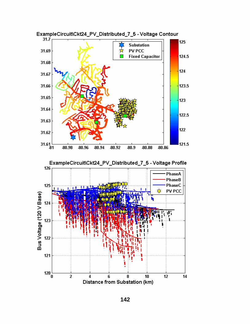
142
143
6.6.2. exampleTimeseriesAnalyses
Timeseries analysis and plots monitor values from the simulation
Syntax exampleTimeseriesAnalyses(basecaseFile,solarScenarioFiles); exampleTimeseriesAnalyses();
Description
Example function for timeseries analysis and monitor plotting for net feeder power and
switching components like LTC and capacitors. Monitors must be setup in the basecaseFile
circuit definition. Place monitors in the desired locations, then use the same names in the code in
this function.
Inputs
basecaseFile - optional input with the link to the OpenDSS file with the circuit.
solarScenarioFiles - optional input with a cell array of links to the OpenDSS files with the
solar scenarios to run
Outputs
none - generates several figures and saves them
Example
Runs the basecase circuit and the distributed solar case
exampleTimeseriesAnalyses('ExampleCircuit\master_ckt24.dss',{'ExampleCircuit\Ckt24_PV_Central_7_5.dss'})
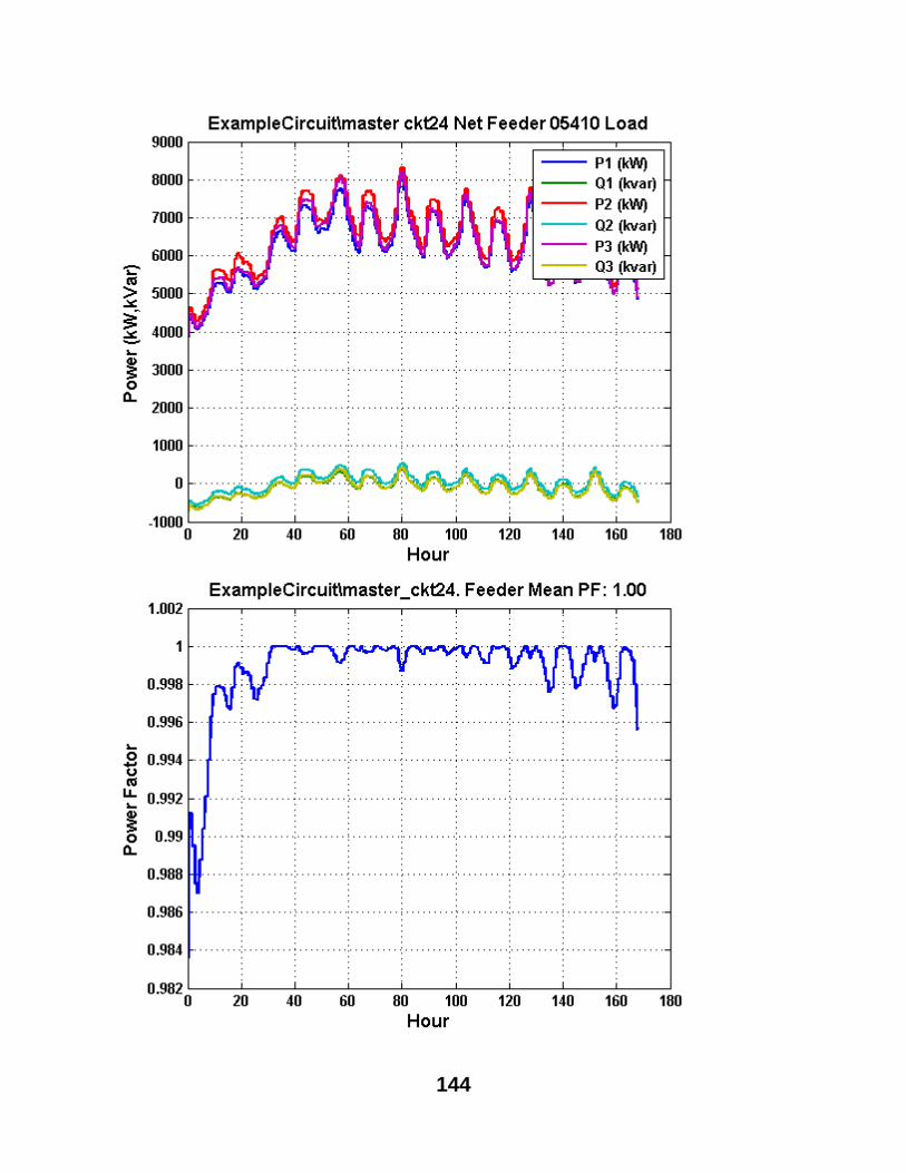
144
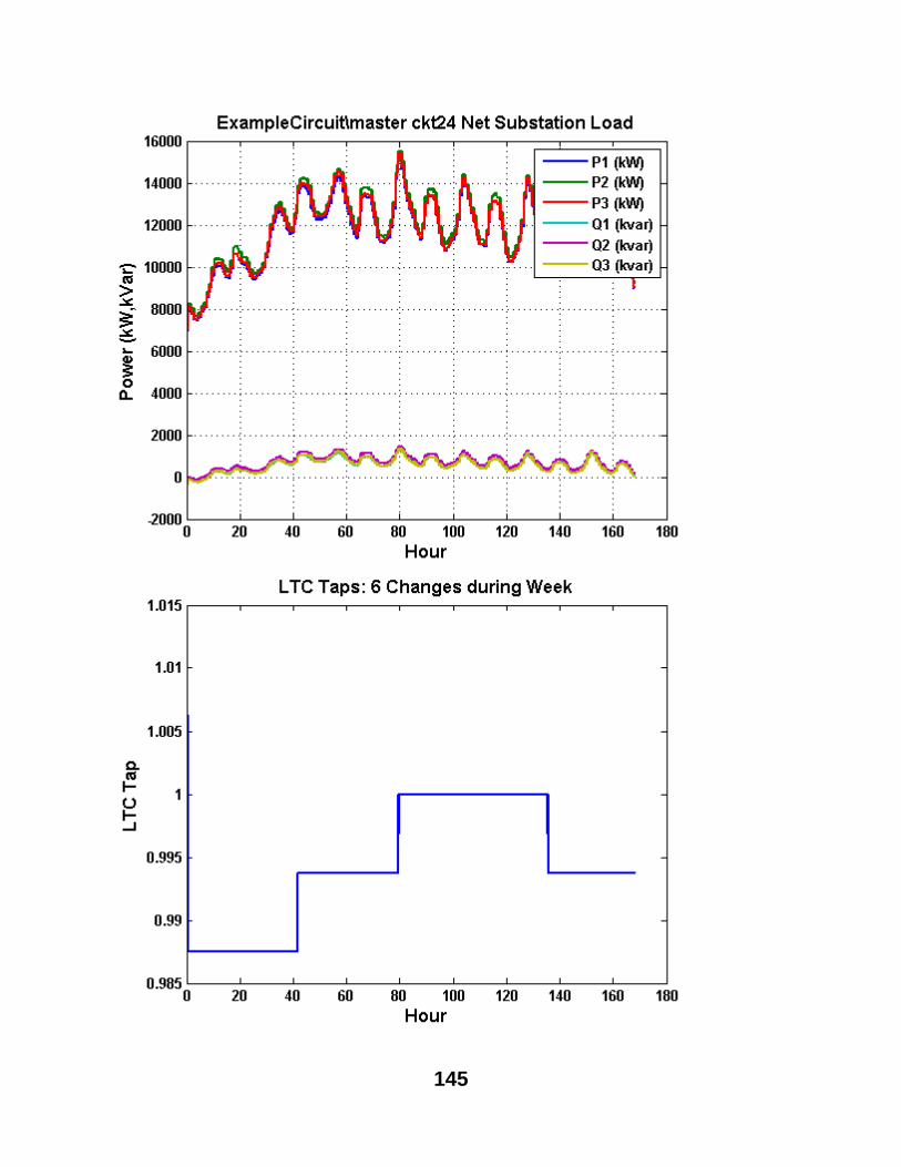
145
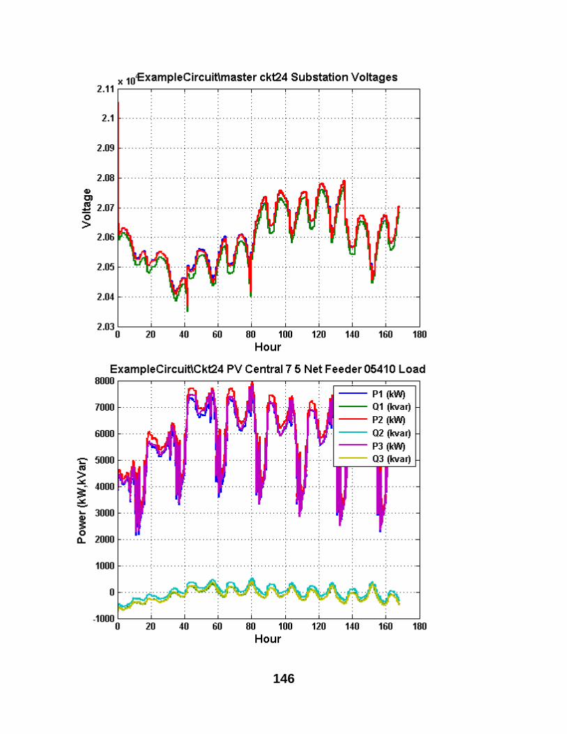
146
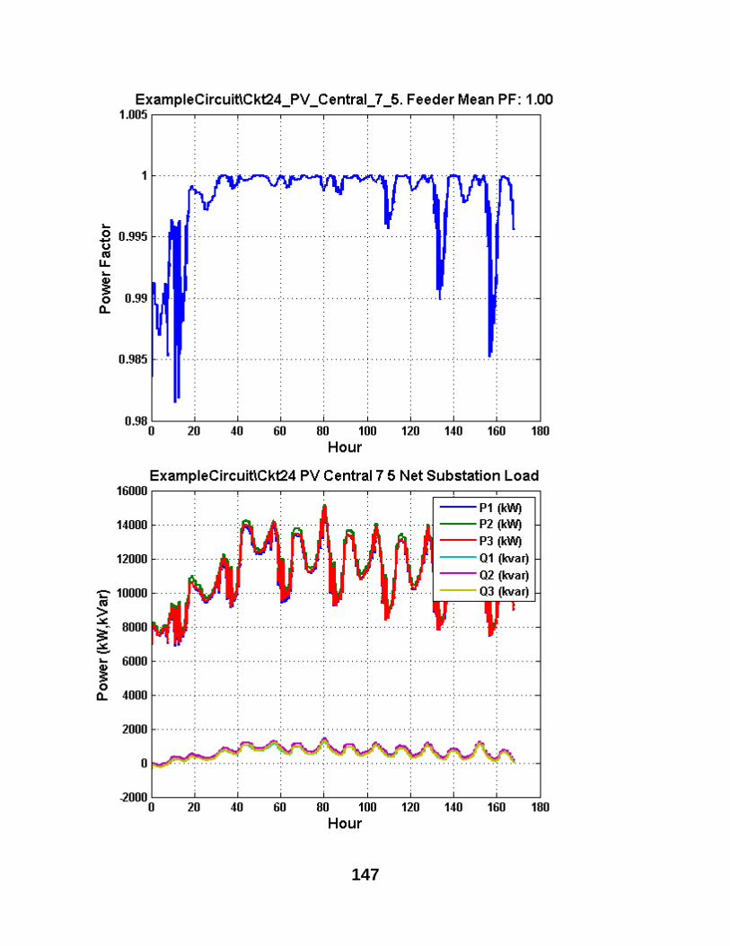
147
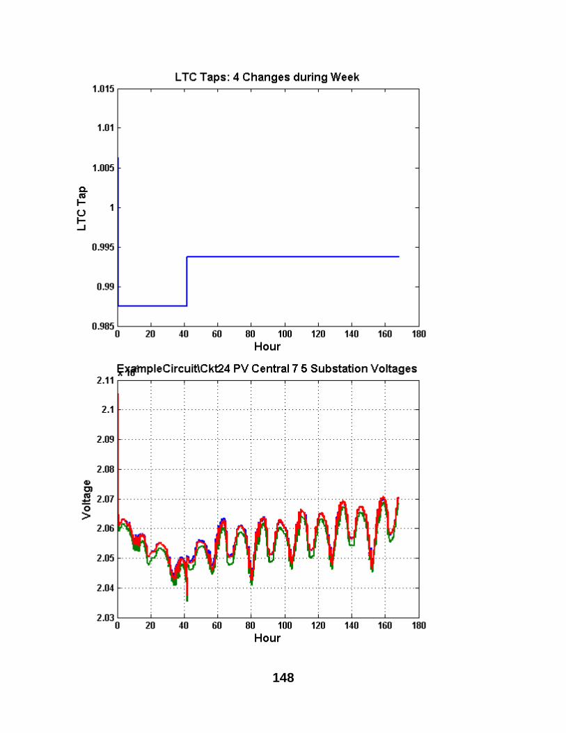
148
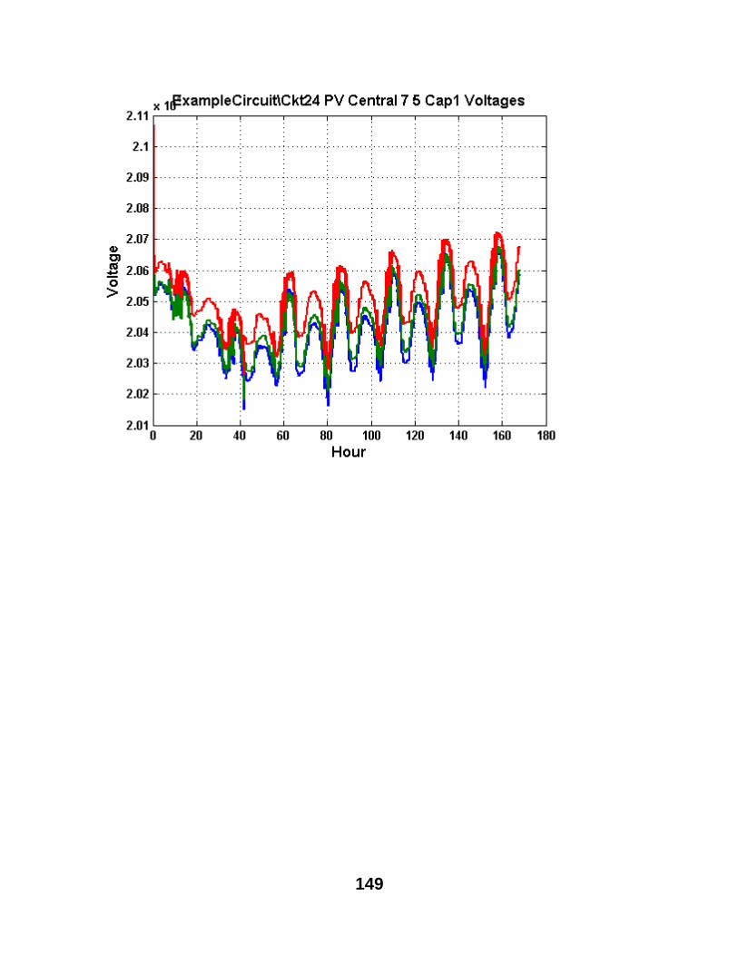
149
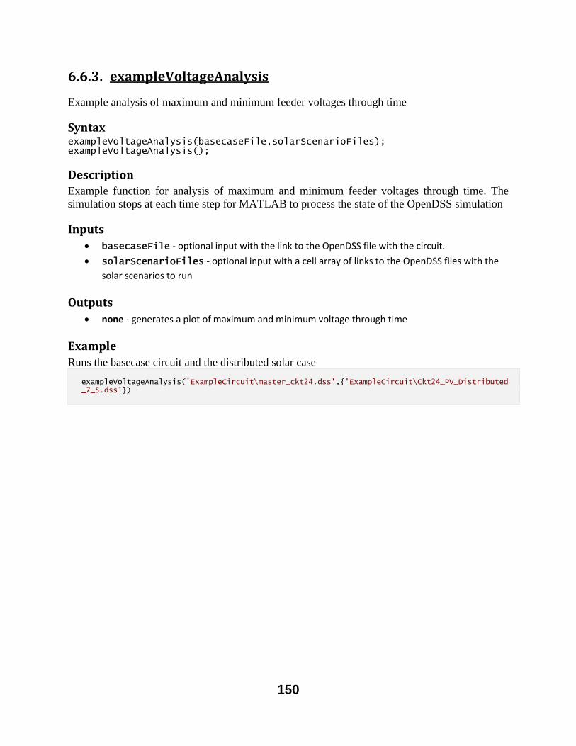
150
6.6.3. exampleVoltageAnalysis
Example analysis of maximum and minimum feeder voltages through time
Syntax exampleVoltageAnalysis(basecaseFile,solarScenarioFiles); exampleVoltageAnalysis();
Description
Example function for analysis of maximum and minimum feeder voltages through time. The
simulation stops at each time step for MATLAB to process the state of the OpenDSS simulation
Inputs
basecaseFile - optional input with the link to the OpenDSS file with the circuit.
solarScenarioFiles - optional input with a cell array of links to the OpenDSS files with the
solar scenarios to run
Outputs
none - generates a plot of maximum and minimum voltage through time
Example
Runs the basecase circuit and the distributed solar case
exampleVoltageAnalysis('ExampleCircuit\master_ckt24.dss',{'ExampleCircuit\Ckt24_PV_Distributed_7_5.dss'})
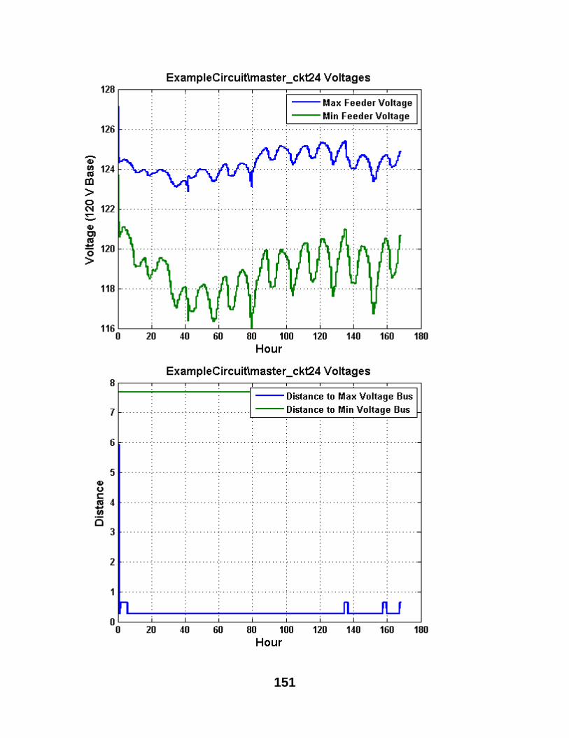
151
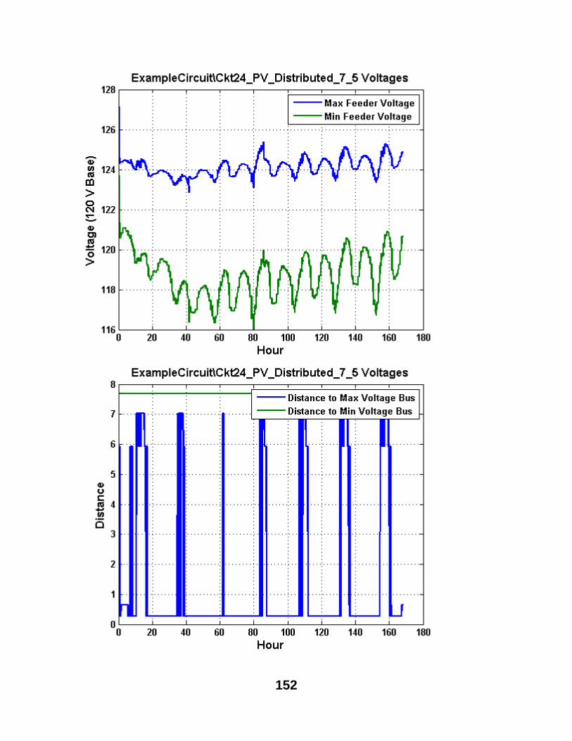
152
153
7. REFERENCES [1] EPRI. (2014). Open Distribution System Simulator. Available:
http://sourceforge.net/projects/electricdss/
[2] K. Coogan, M. J. Reno, and S. Grijalva, "Locational Dependence of PV Hosting Capacity
Correlated with Feeder Load," in IEEE PES Transmission & Distribution Conference &
Exposition, 2014.
[3] M. J. Reno, K. Coogan, S. Grijalva, R. J. Broderick, and J. E. Quiroz, "PV Interconnection Risk
Analysis through Distribution System Impact Signatures and Feeder Zones," in IEEE PES General
Meeting, National Harbor, MD, 2014.
[4] M. J. Reno and K. Coogan, "Grid Integrated Distributed PV (GridPV)," Sandia National Labs
SAND2013-6733, 2013.
[5] M. J. Reno and K. Coogan, "Grid Integrated Distributed PV (GridPV) Version 2," Sandia National
Labs SAND2014-20141, 2014.
[6] J. W. Smith, R. Dugan, and W. Sunderman, "Distribution modeling and analysis of high
penetration PV," in Power and Energy Society General Meeting, 2011 IEEE, 2011, pp. 1-7.
[7] V. Ramachandran, S. K. Solanki, and J. Solanki, "Steady state analysis of three phase unbalanced
distribution systems with interconnection of photovoltaic cells," in Power Systems Conference and
Exposition (PSCE), 2011 IEEE/PES, 2011, pp. 1-7.
[8] J. E. Quiroz and C. P. Cameron, "Technical Analysis of Prospective Photovoltaic Systems in Utah,"
Sandia National Laboratories SAND2012-1366, 2012.
[9] M. J. Reno, A. Ellis, J. Quiroz, and S. Grijalva, "Modeling Distribution System Impacts of Solar
Variability and Interconnection Location," in World Renewable Energy Forum, 2012.
[10] J. Quiroz and M. J. Reno, "Detailed Grid Integration Analysis of Distributed PV," in IEEE
Photovoltaic Specialists Conference, 2012.
[11] R. J. Broderick, J. E. Quiroz, M. J. Reno, A. Ellis, J. Smith, and R. Dugan, "Time Series Power
Flow Analysis for Distribution Connected PV Generation," Sandia National Laboratories
SAND2013-0537, 2013.
[12] M. J. Reno, R. J. Broderick, J. Quiroz, and S. Grijalva, "PV Distribution Interconnection Study
Analysis," in 3rd European American Solar Deployment Conference, 2013.
[13] J. E. Quiroz, M. J. Reno, and R. J. Broderick, "Time Series Simulation of Voltage Regulation
Device Control Modes," in IEEE Photovoltaic Specialists Conference, 2013.
[14] J. W. Smith, W. Sunderman, R. Dugan, and B. Seal, "Smart inverter volt/var control functions for
high penetration of PV on distribution systems," in Power Systems Conference and Exposition
(PSCE), 2011 IEEE/PES, 2011, pp. 1-6.
[15] Google. Google Maps API Family. Available: http://code.google.com/apis/maps/index.html
[16] M. J. Reno, C. W. Hansen, and J. S. Stein, "Global Horizontal Irradiance Clear Sky Models:
Implementation and Analysis," Sandia National Laboratories SAND2012-2389, 2012.
[17] J. S. Stein, C. W. Hansen, and M. J. Reno, "The Variability Index: A New and Novel Metric for
Quantifying Irradiance and PV Output Variability," in World Renewable Energy Forum, 2012.
[18] M. Lave, J. Kleissl, and J. S. Stein, "A Wavelet-Based Variability Model (WVM) for Solar PV
Power Plants," IEEE Transactions on Sustainable Energy, pp. 1-9, 2012.
[19] M. Lave and J. Kleissl, "Testing a wavelet-based variability model (WVM) for solar PV power
plants," in Power and Energy Society General Meeting, 2012 IEEE, 2012, pp. 1-6.
[20] M. Lave and J. Kleissl, "Cloud speed impact on solar variability scaling – Application to the
wavelet variability model," Solar Energy, vol. 91, pp. 11-21, 2013.
[21] M. J. Reno, R. J. Broderick, and S. Grijalva, "Smart Inverter Capabilities for Mitigating Over-
Voltage on Distribution Systems with High Penetrations of PV," in IEEE Photovoltaic Specialists
Conference, Tampa, FL, 2013.

154
[22] J. Seuss, M. J. Reno, R. J. Broderick, and R. G. Harley, "Evaluation of Reactive Power Control
Capabilities of Residential PV in an Unbalanced Distribution Feeder," in IEEE Photovoltaic
Specialists Conference, 2014.
155
8. DISTRIBUTION
1 MS1033 Robert J. Broderick 6112
1 MS1033 Jimmy Quiroz 6112
1 MS1033 Matthew J. Reno 6112
1 MS1033 Abraham Ellis 6112
1 MS0899 Technical Library 9536 (electronic copy)

156