A Demonstration of the Scientific Value of GRUAN Data: the use of GRUAN Uncertainty Estimates in

Trend Analyses

Greg Bodeker and Stefanie KremserBodeker Scientific, Alexandra, New Zealand

Presented at 17th Symposium on Meteorological Observation and Instrumentation, Westminster, 10

June 2014

Overview• Very brief overview of GRUAN

• GRUAN RS92 radiosonde data availability

• RS92 radiosonde measurements at the Lindenberg site which is also the GRUAN Lead Centre

• Things to worry about with trend analyses

• Very first GRUAN trends (but too early)

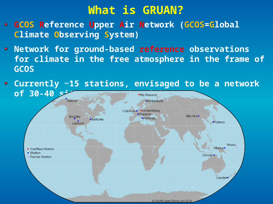
GCOS Reference Upper Air Network (GCOS=Global Climate Observing System)

Network for ground-based reference observations for climate in the free atmosphere in the frame of GCOS

Currently ~15 stations, envisaged to be a network of 30-40 sites across the globe

What is GRUAN?

The goals of GRUAN

The purpose of GRUAN is to:

• Provide long-term high quality climate records;

• Constrain and calibrate data from more spatially-comprehensive global observing systems (including satellites and current radiosonde networks); and

• Fully characterize the properties of the atmospheric column.

Four key user groups of GRUAN data products are identified:

• The climate detection and attribution community.

• The satellite community.

• The atmospheric process studies community.

• The numerical weather prediction (NWP) community.

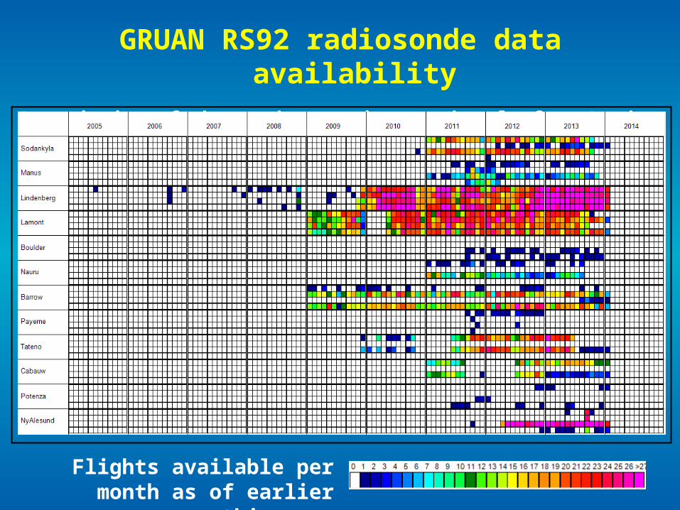
GRUAN RS92 radiosonde data availability

Description of the product coming up shortly from Ruud Dirksen

Flights available per month as of earlier this

year

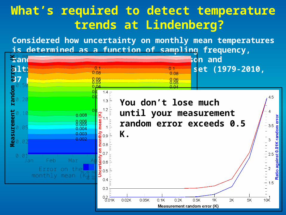
Considered how uncertainty on monthly mean temperatures is determined as a function of sampling frequency, random error on each measurement, season and altitude/pressure. Used NCEPCFSR data set (1979-2010, 37 pressure levels, every 6 hours).

What’s required to detect temperature trends at Lindenberg?

Mea

sure

men

t ra

nd

om

err

or

(K)

0.01

0.02

0.05

0.10

0.20

0.50

1.00

2.00

Jan Feb Mar Apr May Jun Jul Aug Sep Oct Nov Dec

0 0.001

0.002

0.003

0.004

0.005

0.006

0.008

0.01

0.02

0.03

0.04

0.05

0.06

0.08

0.1

0.12

0.14

0.16

0.18

Error on the monthly mean (K)

You don’t lose much until your measurement random error exceeds 0.5 K.

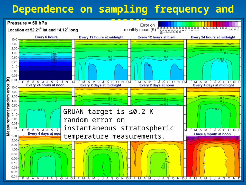
Dependence on sampling frequency and season

GRUAN target is ≤0.2 K random error on instantaneous stratospheric temperature measurements.

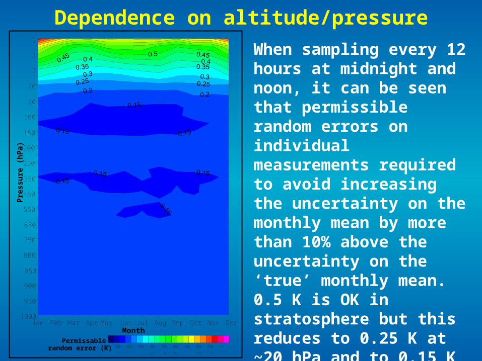
Dependence on altitude/pressure

Month

Pre

ssu

re (

hP

a)

1000

950

900

850

800

750

650

550

450

350

250

200

150

100

50

20

7

3

1

Jan Feb Mar Apr May Jun Jul Aug Sep Oct Nov Dec

0 0.1

0.2

0.3

0.4

0.5

0.6

0.7

0.8

0.9

1Permissablerandom error (K)

When sampling every 12 hours at midnight and noon, it can be seen that permissible random errors on individual measurements required to avoid increasing the uncertainty on the monthly mean by more than 10% above the uncertainty on the ‘true’ monthly mean. 0.5 K is OK in stratosphere but this reduces to 0.25 K at ~20 hPa and to 0.15 K in the free troposphere.

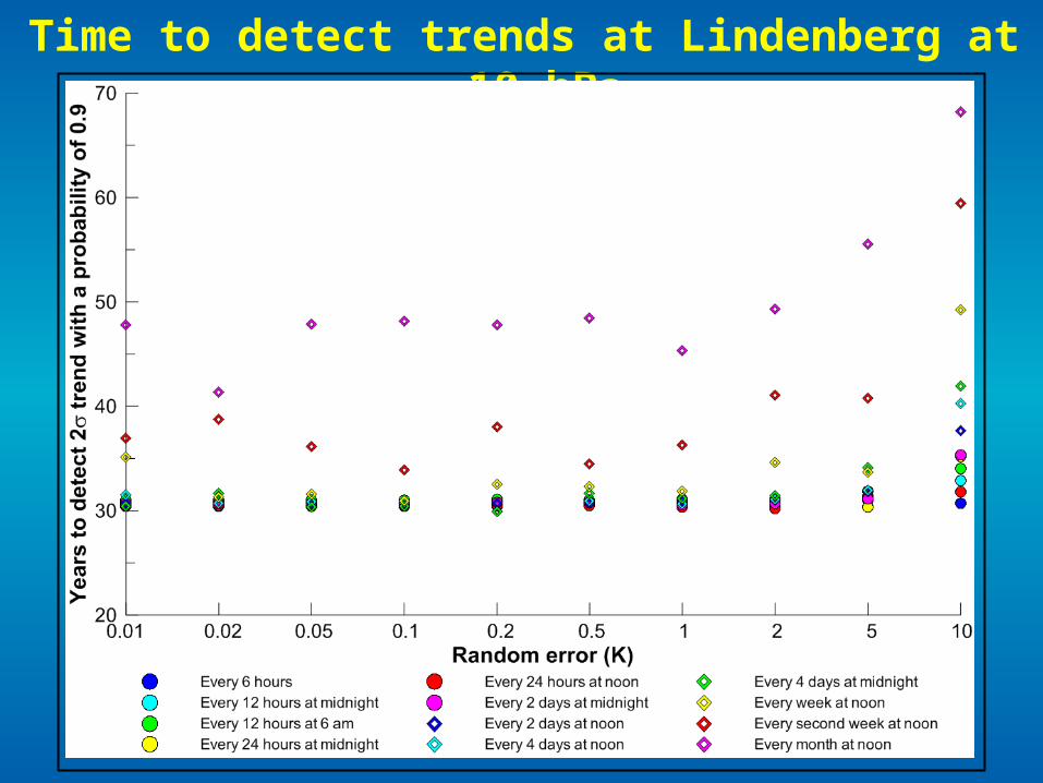
Time to detect trends at Lindenberg at 10 hPa

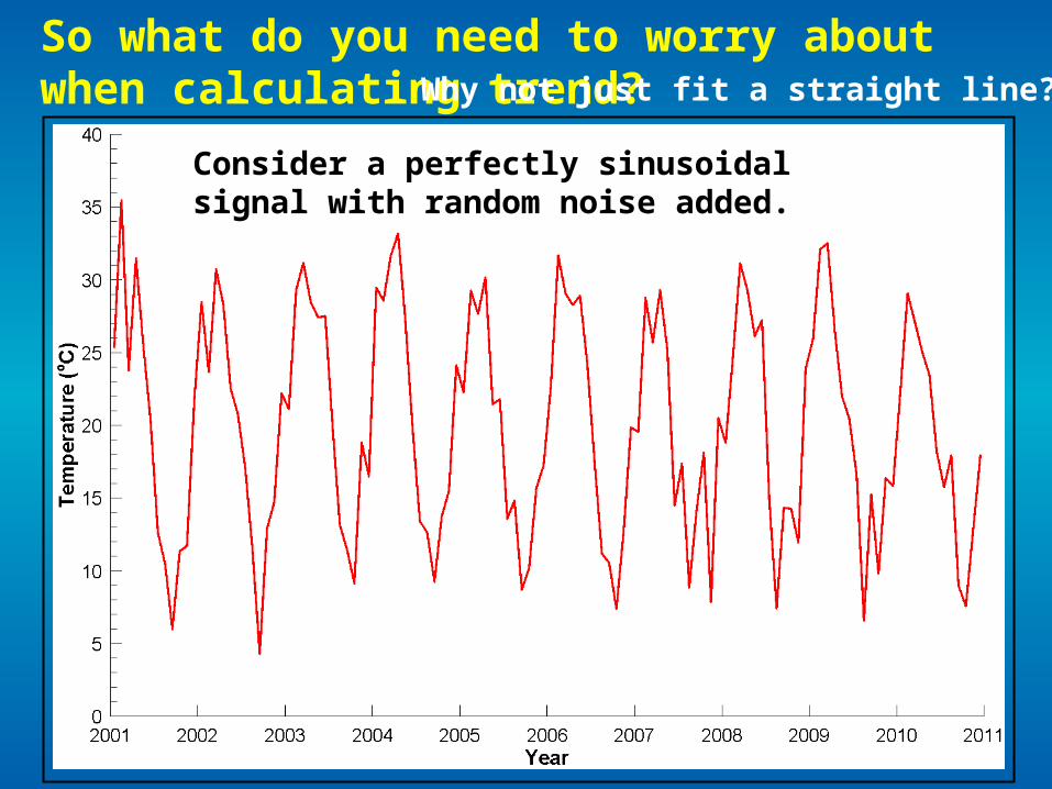
So what do you need to worry about when calculating trend? Why not just fit a straight line?

Consider a perfectly sinusoidal signal with random noise added.

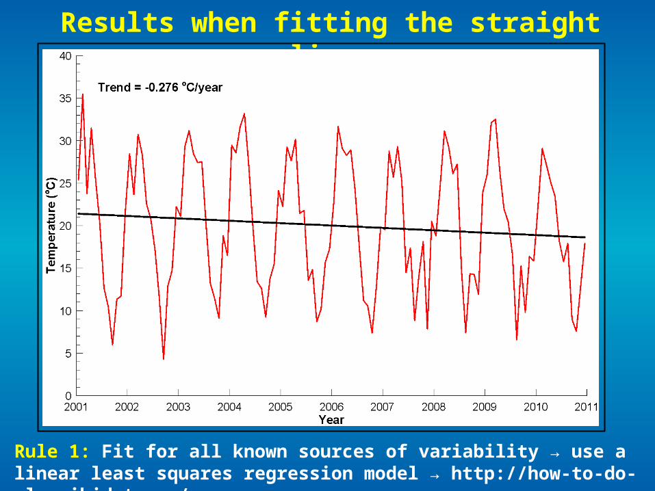
Results when fitting the straight line…

Rule 1: Fit for all known sources of variability → use a linear least squares regression model → http://how-to-do-mlr.wikidot.com/

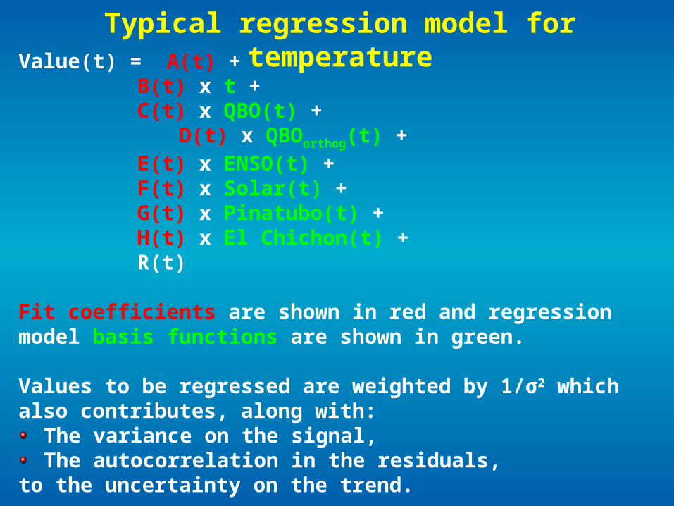
Typical regression model for temperatureValue(t) = A(t) +

B(t) x t +C(t) x QBO(t) +

D(t) x QBOorthog(t) +E(t) x ENSO(t) +F(t) x Solar(t) +G(t) x Pinatubo(t) +H(t) x El Chichon(t) +R(t)

Fit coefficients are shown in red and regression model basis functions are shown in green.

Values to be regressed are weighted by 1/σ2 which also contributes, along with:

The variance on the signal,The autocorrelation in the residuals,

to the uncertainty on the trend.

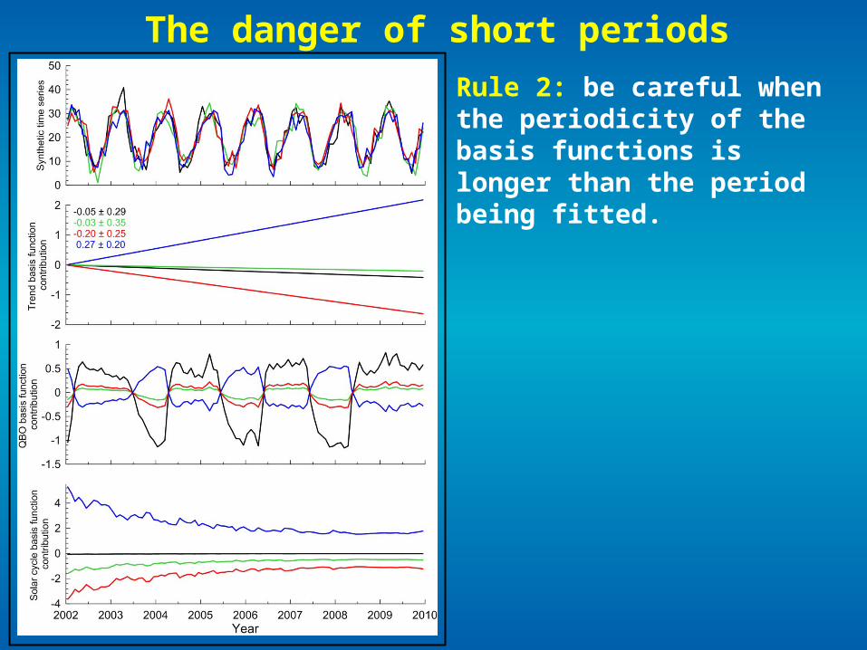
The danger of short periods

Rule 2: be careful when the periodicity of the basis functions is longer than the period being fitted.

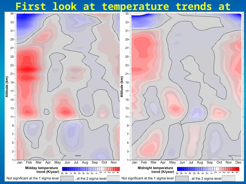
First look at temperature trends at Lindenberg

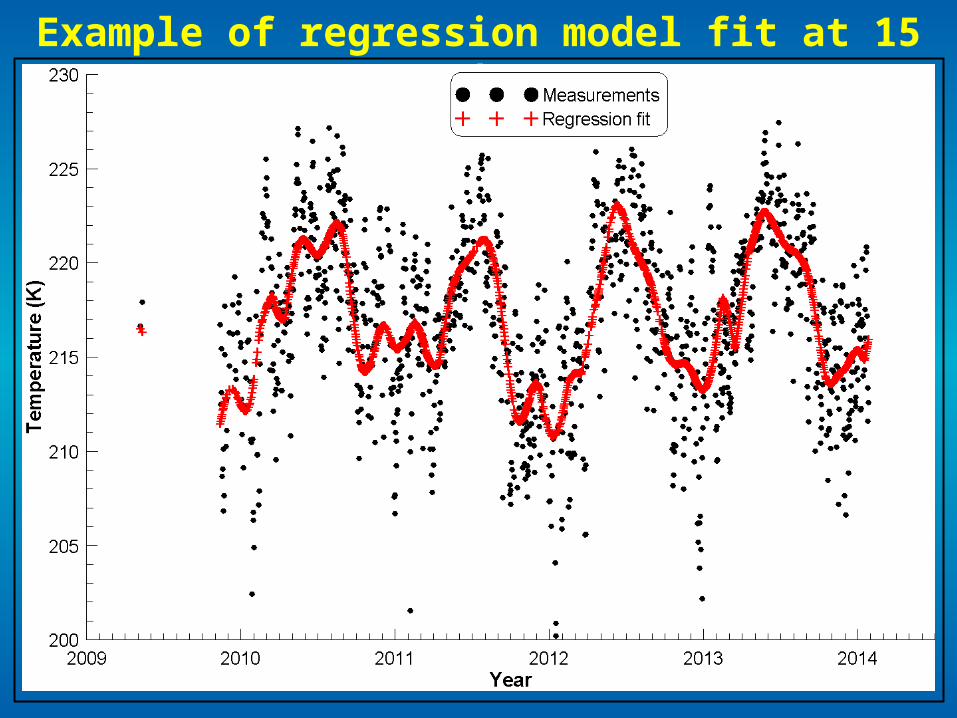
Example of regression model fit at 15 km

Conclusions• There are lots of pitfalls on the path to robust trend

determination. Be careful!

• Uncertainties on GRUAN data allow for trend evaluation including robust uncertainties on the trends.

• Reduced uncertainties on night-time temperature measurements from radiosondes should permit earlier detection of long-term trends.

• The current GRUAN data record is still too short for trend detection.