Chapter 1Introduction

A Green’s function is the response of a medium to a point source and because anyload or charge can be considered a sum of infinitely many such point sources theGreen’s functions play a fundamental role in linear systems. Green’s functions can beconsidered “physically based basis functions adapted to a particular geometry andparticular constraints” [1], and what we do in FE-analysis is that we approximatethese physical basis functions with piecewise polynomials. This is all there is toFE-analysis of linear problems—of course put aside the delicate question of howto choose the best approximate. Testimony to this tight connection between finiteelements and potential theory is the fact that the columns of the inverse stiffnessmatrix are the discrete Green’s functions of the nodal values.

Any (or nearly any) value an FE-program outputs has been processed by thesenumerical influence functions and the kernel in these influence functions are theapproximate Green’s functions pieced together from the nodal basis functions.

The better an FE-mesh can react to the point loads which generate the Green’sfunctions the better the accuracy of the FE-solution. That is the shapes a mesh canassume, its kinematics, the quality of the Green’s functions which can be generatedon the mesh, ultimately determines the quality of an FE-solution.

And because any Green’s function strongly depends on the model parameters, theslightest change in a coefficient, say on a stretch of only 0.1 m, will affect the wholefunction, the sensitivities of a model can be made visible by plotting the updatedGreen’s function and so the user gets an impression of the difficulties involved inevaluating certain functionals. The machinery, so to speak, which the FE-programuses, can be laid bare. FE-analysis becomes transparent, becomes visual.

What is nice about Green’s functions and finite elements is that the calculation ofGreen’s functions is easy to implement in any existing code. Detailed instructionson how to calculate influence functions with FE-programs close the chapter.

F. Hartmann, Green’s Functions and Finite Elements, 1DOI: 10.1007/978-3-642-29523-2_1, © Springer-Verlag Berlin Heidelberg 2013

2 1 Introduction

1.1 What are Green’s Functions?

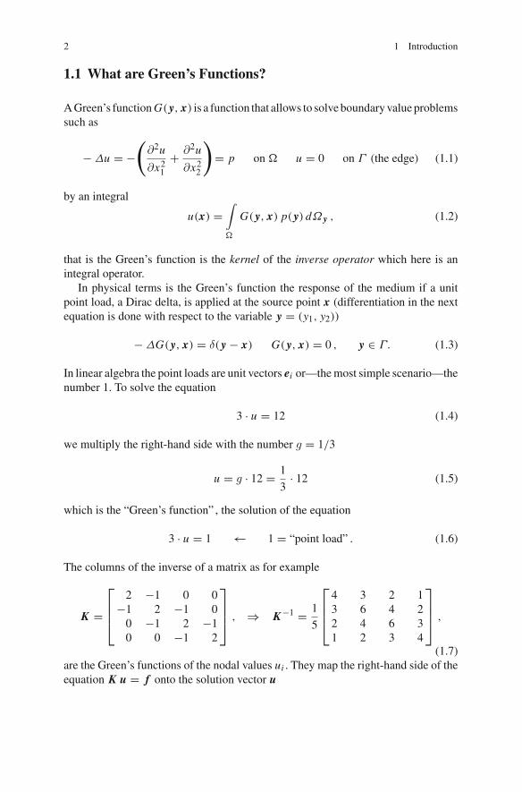
A Green’s function G( y, x) is a function that allows to solve boundary value problemssuch as

−Δu = −(∂2u

∂x21

+ ∂2u

∂x22

)= p on � u = 0 on Γ (the edge) (1.1)

by an integral

u(x) =∫�

G( y, x) p( y) dΩ y , (1.2)

that is the Green’s function is the kernel of the inverse operator which here is anintegral operator.

In physical terms is the Green’s function the response of the medium if a unitpoint load, a Dirac delta, is applied at the source point x (differentiation in the nextequation is done with respect to the variable y = (y1, y2))

−ΔG( y, x) = δ( y − x) G( y, x) = 0 , y ∈ Γ. (1.3)

In linear algebra the point loads are unit vectors ei or—the most simple scenario—thenumber 1. To solve the equation

3 · u = 12 (1.4)

we multiply the right-hand side with the number g = 1/3

u = g · 12 = 1

3· 12 (1.5)

which is the “Green’s function” , the solution of the equation

3 · u = 1 ← 1 = “point load” . (1.6)

The columns of the inverse of a matrix as for example

K =

⎡⎢⎢⎣

2 −1 0 0−1 2 −1 0

0 −1 2 −10 0 −1 2

⎤⎥⎥⎦ , ⇒ K−1 = 1

5

⎡⎢⎢⎣

4 3 2 13 6 4 22 4 6 31 2 3 4

⎤⎥⎥⎦ ,

(1.7)are the Green’s functions of the nodal values ui . They map the right-hand side of theequation K u = f onto the solution vector u

1.1 What are Green’s Functions? 3

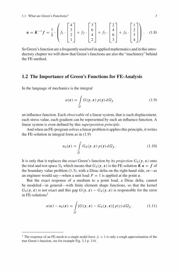
u = K−1 f = 1

5·

⎛⎜⎜⎝ f1 ·

⎡⎢⎢⎣

4321

⎤⎥⎥⎦+ f2 ·

⎡⎢⎢⎣

3642

⎤⎥⎥⎦+ f3 ·

⎡⎢⎢⎣

2463

⎤⎥⎥⎦+ f4 ·

⎡⎢⎢⎣

1234

⎤⎥⎥⎦

⎞⎟⎟⎠ . (1.8)

So Green’s function are a frequently used tool in applied mathematics and in this intro-ductory chapter we will show that Green’s functions are also the “machinery” behindthe FE-method.

1.2 The Importance of Green’s Functions for FE-Analysis

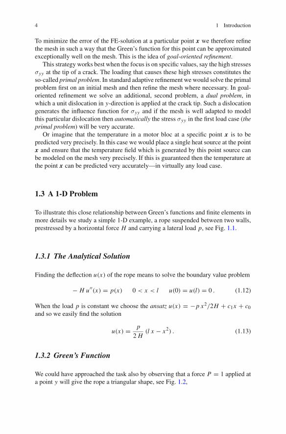
In the language of mechanics is the integral

u(x) =∫Ω

G( y, x) p( y) dΩ y (1.9)

an influence function. Each observable of a linear system, that is each displacement,each stress value, each gradient can be represented by such an influence function. Alinear system is even defined by this superposition principle.

And when an FE-program solves a linear problem it applies this principle, it writesthe FE-solution in integral form as in (1.9)

uh(x) =∫Ω

Gh( y, x) p( y) dΩ y . (1.10)

It is only that it replaces the exact Green’s function by its projection Gh( y, x) ontothe trial and test space Vh which means that Gh( y, x) is the FE-solution K u = f ofthe boundary value problem (1.3), with a Dirac delta on the right-hand side, or—asan engineer would say—when a unit load P = 1 is applied at the point x.

But the exact response of a medium to a point load, a Dirac delta, cannotbe modeled—in general—with finite element shape functions, so that the kernelGh( y, x) is not exact and this gap G( y, x) − Gh( y, x) is responsible for the errorin FE-solutions1

u(x)− uh(x) =∫Ω

[G( y, x)− Gh( y, x)] p(y) dΩ y . (1.11)

1 The response of an FE-mesh to a single nodal force fi = 1 is only a rough approximation of thetrue Green’s function, see for example Fig. 3.3 p. 114.

4 1 Introduction

To minimize the error of the FE-solution at a particular point x we therefore refinethe mesh in such a way that the Green’s function for this point can be approximatedexceptionally well on the mesh. This is the idea of goal-oriented refinement.

This strategy works best when the focus is on specific values, say the high stressesσyy at the tip of a crack. The loading that causes these high stresses constitutes theso-called primal problem. In standard adaptive refinement we would solve the primalproblem first on an initial mesh and then refine the mesh where necessary. In goal-oriented refinement we solve an additional, second problem, a dual problem, inwhich a unit dislocation in y-direction is applied at the crack tip. Such a dislocationgenerates the influence function for σyy and if the mesh is well adapted to modelthis particular dislocation then automatically the stress σyy in the first load case (theprimal problem) will be very accurate.

Or imagine that the temperature in a motor bloc at a specific point x is to bepredicted very precisely. In this case we would place a single heat source at the pointx and ensure that the temperature field which is generated by this point source canbe modeled on the mesh very precisely. If this is guaranteed then the temperature atthe point x can be predicted very accurately—in virtually any load case.

1.3 A 1-D Problem

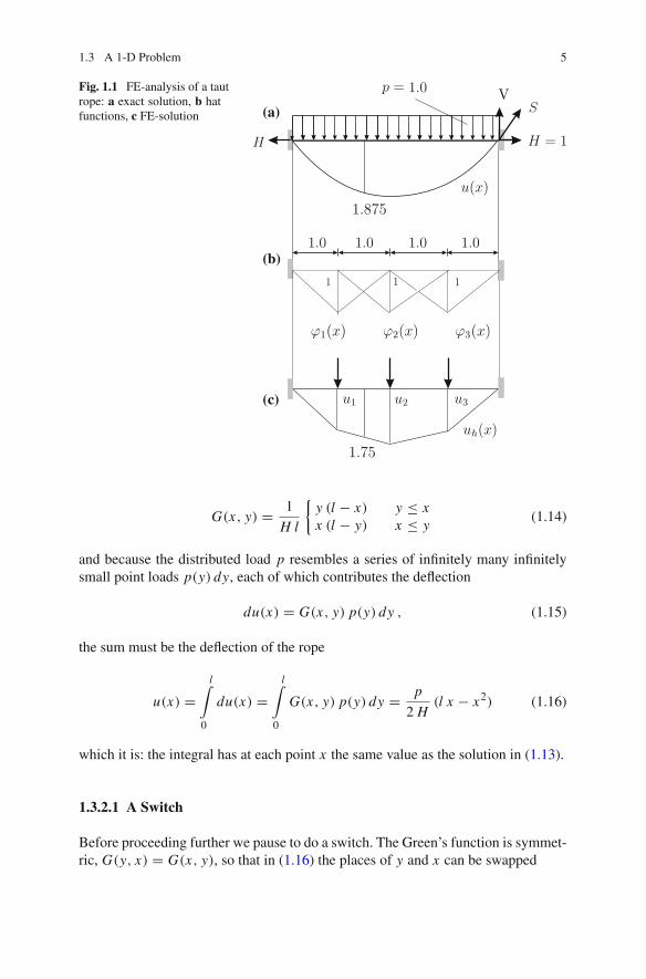
To illustrate this close relationship between Green’s functions and finite elements inmore details we study a simple 1-D example, a rope suspended between two walls,prestressed by a horizontal force H and carrying a lateral load p, see Fig. 1.1.

1.3.1 The Analytical Solution

Finding the deflection u(x) of the rope means to solve the boundary value problem

− H u′′(x) = p(x) 0 < x < l u(0) = u(l) = 0 . (1.12)

When the load p is constant we choose the ansatz u(x) = −p x2/2H + c1x + c0and so we easily find the solution

u(x) = p

2 H(l x − x2) . (1.13)

1.3.2 Green’s Function

We could have approached the task also by observing that a force P = 1 applied ata point y will give the rope a triangular shape, see Fig. 1.2,

1.3 A 1-D Problem 5

Fig. 1.1 FE-analysis of a tautrope: a exact solution, b hatfunctions, c FE-solution (a)

(b)

(c)

G(x, y) = 1

H l

{y (l − x) y ≤ xx (l − y) x ≤ y

(1.14)

and because the distributed load p resembles a series of infinitely many infinitelysmall point loads p(y) dy, each of which contributes the deflection

du(x) = G(x, y) p(y) dy , (1.15)

the sum must be the deflection of the rope

u(x) =l∫

0

du(x) =l∫

0

G(x, y) p(y) dy = p

2 H(l x − x2) (1.16)

which it is: the integral has at each point x the same value as the solution in (1.13).

1.3.2.1 A Switch

Before proceeding further we pause to do a switch. The Green’s function is symmet-ric, G(y, x) = G(x, y), so that in (1.16) the places of y and x can be swapped

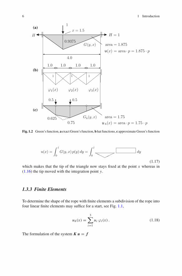
6 1 Introduction

u

(a)

(b)

(c)

Fig. 1.2 Green’s function, a exact Green’s function, b hat functions, c approximate Green’s function

(1.17)which makes that the tip of the triangle now stays fixed at the point x whereas in(1.16) the tip moved with the integration point y.

1.3.3 Finite Elements

To determine the shape of the rope with finite elements a subdivision of the rope intofour linear finite elements may suffice for a start, see Fig. 1.1,

uh(x) =3∑

i=1

ui ϕi (x) . (1.18)

The formulation of the system K u = f

1.3 A 1-D Problem 7⎡⎣ 2 −1 0−1 2 −1

0 −1 2

⎤⎦

⎡⎣ u1

u2u3

⎤⎦ =

⎡⎣ 1

11

⎤⎦ . (1.19)

and finding its solutionu1 = u3 = 1.5 u2 = 2.0 (1.20)

is standard and so we easily determine that

uh(x) = 1.5 · ϕ1(x)+ 2.0 · ϕ2(x)+ 1.5 · ϕ3(x) (1.21)

is the best approximation to u(x) with four elements in terms of the strain energymetric.

1.3.4 Finite Elements and Green’s Function

Now let us try a novel approach, a combination of finite elements and Green’s func-tion.

The Green’s function G(y, x) is the shape of the rope when a force P = 1is applied at x that is the Green’s function is the solution of the boundary valueproblem

− Hd2

dy2 G(y, x) = δ(y − x) G(0, x) = G(l, x) = 0 . (1.22)

What happens if this boundary value problem is solved with finite elements andthe FE-solution Gh(y, x) instead of the exact kernel G(y, x) is substituted into theinfluence function (1.16)? Which effect does this have on the influence function?

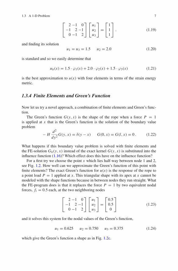
For a first try we choose the point x which lies half-way between node 1 and 2,see Fig. 1.2. How well can we approximate the Green’s function of this point withfinite elements? The exact Green’s function for u(x) is the response of the rope toa point load P = 1 applied at x . This triangular shape with its apex at x cannot bemodeled with the shape functions because in between nodes they run straight. Whatthe FE-program does is that it replaces the force P = 1 by two equivalent nodalforces, fi = 0.5 each, at the two neighboring nodes

⎡⎣ 2 −1 0−1 2 −1

0 −1 2

⎤⎦

⎡⎣ u1

u2u3

⎤⎦ =

⎡⎣ 0.5

0.50

⎤⎦ (1.23)

and it solves this system for the nodal values of the Green’s function,

u1 = 0.625 u2 = 0.750 u3 = 0.375 (1.24)

which give the Green’s function a shape as in Fig. 1.2c.

8 1 Introduction

This is of course not the correct shape, the peak under the point load is missing,and so the substitute influence function (1.16) the integral

1.75 =l∫

0

Gh(y, x) p(y) dy (1.25)

gives a wrong value—the true value is 1.875. But when we look closer then wefind—to our surprise—that the value 1.75 is exactly the value of the FE-solution atthis point, see Fig. 1.1c.

And if we repeat this experiment at other points of the rope we always find thatthe integral of the approximate Green’s function Gh(y, x) and the distributed loadp is exactly the value of the FE-solution at this point

uh(x) =3∑

i=1

ui ϕi (x) =l∫

0

Gh(y, x) p(y) dy . (1.26)

So it must be true that an FE-program uses the approximate Green’s functions tocalculate the deflection uh(x) of the rope.

But does’nt an FE-program calculate the nodal values u—and therewith alsoindirectly the values in between—by solving the equation K u = f ? This is trueas well but it does not contradict the previous statement. Both statements are true.2

The nodal values ui the FE-program outputs—and any other value in between aswell—are as large as if the FE-program had calculated them with the approximateGreen’s function which can be generated on the mesh.

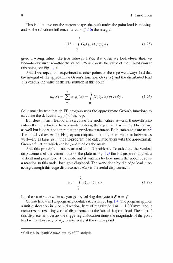
And this principle is not restricted to 1-D problems. To calculate the verticaldisplacement of the center node of the plate in Fig. 1.3 the FE-program applies avertical unit point load at the node and it watches by how much the upper edge asa reaction to this nodal load gets displaced. The work done by the edge load p onacting through this edge displacement η(x) is the nodal displacement

uy =l∫

0

p(x) η(x) dx . (1.27)

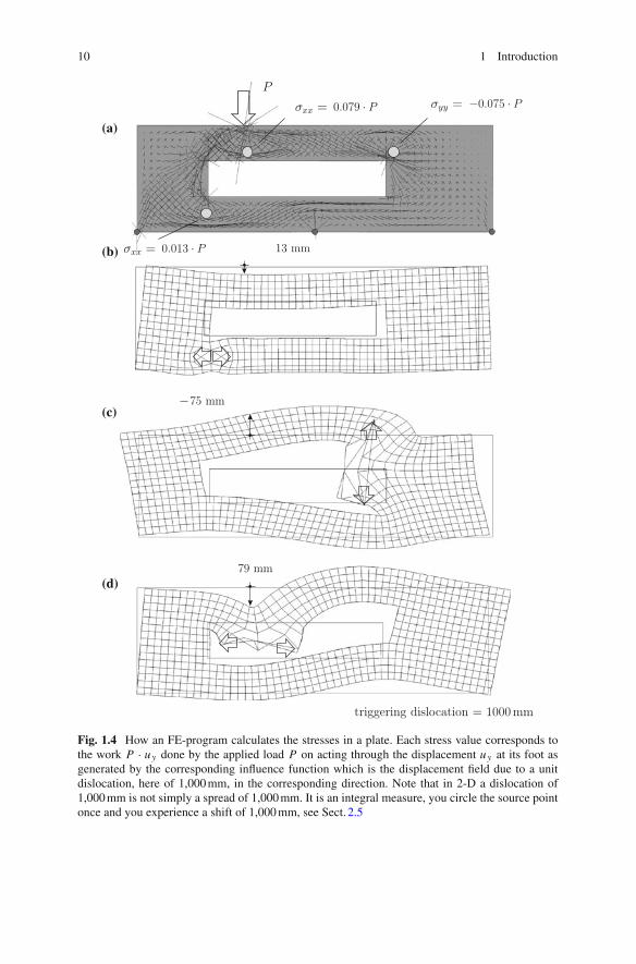
It is the same value ui = uy you get by solving the system K u = f .Or watch how an FE-program calculates stresses, see Fig. 1.4. The program applies

a unit dislocation in x or y direction, here of magnitude 1 m = 1,000 mm, and itmeasures the resulting vertical displacement at the foot of the point load. The ratio ofthis displacement versus the triggering dislocation times the magnitude of the pointload is the stress σxx or σyy respectively at the source point

2 Call this the “particle-wave” duality of FE-analysis.

1.3 A 1-D Problem 9

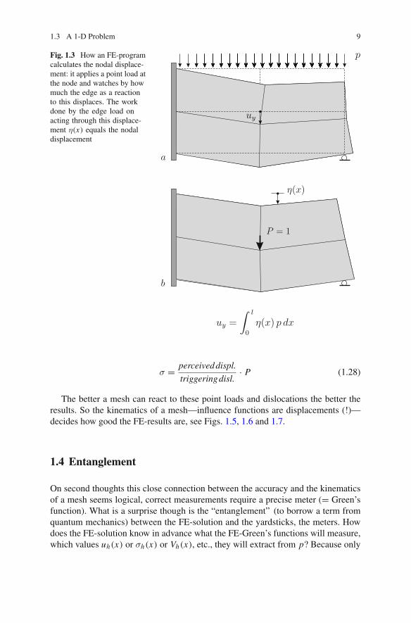
Fig. 1.3 How an FE-programcalculates the nodal displace-ment: it applies a point load atthe node and watches by howmuch the edge as a reactionto this displaces. The workdone by the edge load onacting through this displace-ment η(x) equals the nodaldisplacement

σ = perceiveddispl.

triggeringdisl.· P (1.28)

The better a mesh can react to these point loads and dislocations the better theresults. So the kinematics of a mesh—influence functions are displacements (!)—decides how good the FE-results are, see Figs. 1.5, 1.6 and 1.7.

1.4 Entanglement

On second thoughts this close connection between the accuracy and the kinematicsof a mesh seems logical, correct measurements require a precise meter (= Green’sfunction). What is a surprise though is the “entanglement” (to borrow a term fromquantum mechanics) between the FE-solution and the yardsticks, the meters. Howdoes the FE-solution know in advance what the FE-Green’s functions will measure,which values uh(x) or σh(x) or Vh(x), etc., they will extract from p? Because only

10 1 Introduction

(a)

(b)

(c)

(d)

Fig. 1.4 How an FE-program calculates the stresses in a plate. Each stress value corresponds tothe work P · uy done by the applied load P on acting through the displacement uy at its foot asgenerated by the corresponding influence function which is the displacement field due to a unitdislocation, here of 1,000 mm, in the corresponding direction. Note that in 2-D a dislocation of1,000 mm is not simply a spread of 1,000 mm. It is an integral measure, you circle the source pointonce and you experience a shift of 1,000 mm, see Sect. 2.5

1.4 Entanglement 11

(a)

(b)

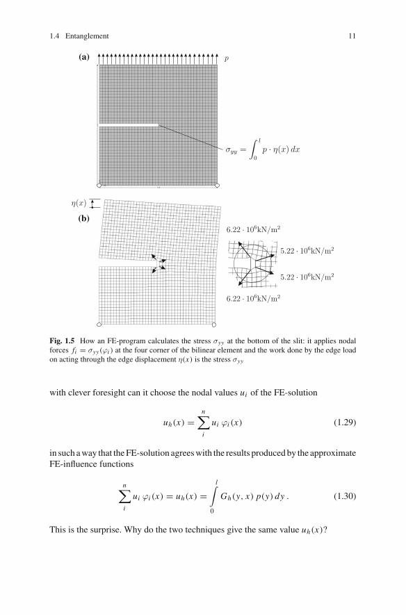
Fig. 1.5 How an FE-program calculates the stress σyy at the bottom of the slit: it applies nodalforces fi = σyy(ϕi ) at the four corner of the bilinear element and the work done by the edge loadon acting through the edge displacement η(x) is the stress σyy

with clever foresight can it choose the nodal values ui of the FE-solution

uh(x) =n∑i

ui ϕi (x) (1.29)

in such a way that the FE-solution agrees with the results produced by the approximateFE-influence functions

n∑i

ui ϕi (x) = uh(x) =l∫

0

Gh(y, x) p(y) dy . (1.30)

This is the surprise. Why do the two techniques give the same value uh(x)?

12 1 Introduction

(a)

(b)

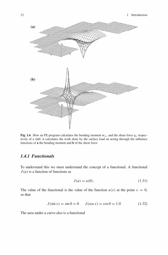
Fig. 1.6 How an FE-program calculates the bending moment mxx and the shear force qx respec-tively of a slab: it calculates the work done by the surface load on acting through the influencefunctions of a the bending moment and b of the shear force

1.4.1 Functionals

To understand this we must understand the concept of a functional. A functionalJ (u) is a function of functions as

J (u) = u(0) . (1.31)

The value of the functional is the value of the function u(x) at the point x = 0,so that

J (sin x) = sin 0 = 0 J (cos x) = cos 0 = 1.0 (1.32)

The area under a curve also is a functional

1.4 Entanglement 13

J (u) =π∫

0

u(x) dx J (sin x) =π∫

0

sin x dx = 2 . (1.33)

Assume you are learning a new programming language and your first assignment isto write a small program to calculate the deflection of a rope subjected to varioustypes of loads p. For a test the instructor asks you for the deflection at a specificpoint x . In an abstract sense the teacher is asking for the value of the functional

J (u) = u(x) . (1.34)

How does the program calculate u(x)? You—as the author of the program—will saythat the program calls the subroutine where u(x) is stored and that it simply looksup the value of u.

But a point value such as u(x) can also be thought to come from the applicationof a Dirac delta to the function u

1 · u(x) =l∫

0

δ(y − x) u(y) dy (1.35)

that is when a unit point load acts through u(x). On first view this seems to complicatematters unnecessarily: “What sense is there in interpreting a function call—the simpleevaluation of a function—an application of a Dirac delta?”

But Betti would argue that when a Dirac delta is applied to the solution u thenthis is the same as if the product of the Green’s function and the right-hand side p,the applied load, is integrated

1 · u(x) =l∫

0

δ(y − x) u(y) dy =l∫

0

G(y, x) p(y) dy . (1.36)

And Betti is right, indeed, the work done by the point load δ(y − x) on actingthrough u(x) is equal to the work done by the distributed load p on acting throughthe displacement G(y, x) caused by the point load. This is the important step.

Saying a solution has at a point x the value u(x) is saying the functional J (u) =u(x) has the value u(x). Each observable is identical with a functional. A supportreaction RA, the shear force V (x), the second derivative u′′(x), a nodal value ui , allthese are functionals.

How can Betti’s logic be extended to handle these various functionals? To do thiswe first generalize the idea of the Dirac delta by claiming that any linear functional,as the following three functionals

14 1 Introduction

50 cm

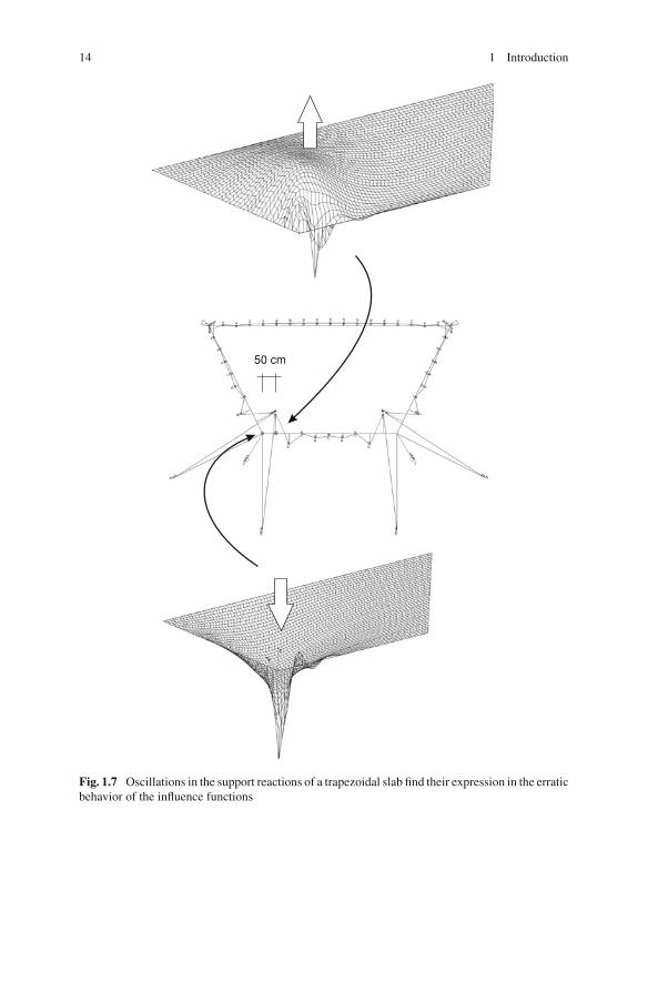
Fig. 1.7 Oscillations in the support reactions of a trapezoidal slab find their expression in the erraticbehavior of the influence functions

1.4 Entanglement 15

Ja(u) = u′(0) =l∫

0

δa(y − x) u(y) dy (1.37)

Jb(u) =l∫

0

u(x) dx =l∫

0

δb(y − x) u(y) dy (1.38)

Jc(u) = u′(x)+ u(x) =l∫

0

δc(y − x) u(y) dy etc. , (1.39)

can be written as integrals between certain Dirac deltas and the solution u. Whatthese Dirac deltas δa, δb, δc look like is not important. It suffices to postulate thatthey exist.

What is important is that each of these integrals can be interpreted as an expressionof exterior work: a certain point load δ(y − x) is acting through u and contributes acertain amount of work W1,2 = J (u). And according to Betti’s theorem this workmust be equal to the work W2,1, (we switch the indices), done by the right-hand sidep, belonging to u, on acting through the shape G(y, x) produced by the Dirac deltaδ(y − x)

J (u) =l∫

0

δ(y − x) u(y) dy = W1,2 = W2,1 =l∫

0

G(y, x) p(y) dy . (1.40)

This is the basic logic. This is duality.The function G(y, x) (or kernel) is called the Riesz element of J (u). In physical

terms it is the response of the medium to the “point load”δ(y − x), the Dirac delta.It is essential that (1.40) remains valid3 if the two exact solutions G and u are

replaced by their FE-approximations while the loads δ and p stay the same

W h1,2 =

l∫0

δ(y − x) uh↑(y) dy =

l∫0

Gh↑(y, x) p(y) dy = W h

2,1 (1.41)

because this invariance implies, see Tottenham’s equation p. 116,

J (uh) =l∫

0

Gh(y, x) p(y) dy (1.42)

3 see Betti’s Theorem Extended, p. 114.

16 1 Introduction

which is the key result. It means that in linear FE-analysis any observable is theL2-scalar product (integral) between the right-hand side p and the projection Gh ofthe Green’s function belonging to the observable onto the test and trial space Vh .

In this sense FE-analysis is “consistent” . While the exact solution u is projectedonto the FE-solution uh and—parallel to this—the exact kernels G onto FE-kernelsGh , the bond between u and the kernels G is never lost. It is inherited by uh and thekernels Gh . While the kernel G maps p onto J (u), the projected kernel Gh maps ponto J (uh), the functional value of the projection uh

J (u) =l∫

0

G(y, x) p(y) dy (1.43)

J (uh) =l∫

0

Gh(y, x) p(y) dy . (1.44)

It is only that in FE-analysis the mapping is distorted. The “lens” Gh(y, x) shouldsend the “beam” p onto the point J (u) but instead it sends it to a slightly differentspot J (uh) on the real axis.

1.4.2 Proof

What we call entanglement is of course simply a consequence of the fact that theunderlying differential equation is self-adjoint and therefore the FE-matrix K sym-metric. This guarantees (1.42).

To exemplify this let the J be the point functional J (u) = u(x). The Green’sfunction G(y, x) of this functional is the solution of the boundary value problem

− Hd2

dy2 G(y, x) = δ(y − x) G(0, x) = G(l, x) = 0 (1.45)

where the Dirac delta represents a point force in the weak sense. Like a real pointforce it is zero almost everywhere and the work done by δ(y − x) on acting througha virtual displacement v is v(x)

δ(y − x) = 0 y �= x (1.46)l∫

0

δ(y − x) v(y) dy = v(x) x ∈ (0, l) . (1.47)

This is what weak means, one studies something by observing its effect on a set oftest functions, i.e. virtual displacements.

1.4 Entanglement 17

The FE-solution of the boundary value problem (1.45), the FE-Green’s function,has the form

Gh(y, x) =∑

i

gi (x)ϕi (y) (1.48)

where the vector g of the nodal displacements (gi ≡ ui ) is the solution of the system

K g = j (1.49)

and where j is the vector of equivalent nodal forces for the Green’s function,

ji = J (ϕi ) (1.50)

or given that J (u) = u(x)

ji = J (ϕi ) = ϕi (x) . (1.51)

So in contrast to the standard FE-notation we use gi for the nodal values of the Green’sfunction and the equivalent nodal forces which generate the Green’s function we callji because the forces are just the values of the functional applied to the single shapefunctions ϕi .

The following theorem summarizes these results.

Theorem 1.1 (The central equation).

uh(x) =l∫

0

Gh(y, x) p(y) dy =l∫

0

∑i

gi (x)ϕi (y) p(y) dy =∑

i

gi (x) fi

= gT f = gT K u = gT K T u = j T u =∑

i

ji ui

=∑

i

ϕi (x) ui =l∫

0

∑i

ui ϕi (y) δ(y − x) dy =l∫

0

uh(y) δ(y − x) dy .

(1.52)

The displacement uh(x) is the scalar product, gT f , between the nodal displacementsof the Green’s function and the equivalent nodal forces of the load p or—vice versa—the scalar product, j T u, between the nodal displacements of the FE-solution uh andthe nodal forces ji of the Green’s function

18 1 Introduction

uh(x) =

⎧⎪⎪⎪⎪⎪⎪⎨⎪⎪⎪⎪⎪⎪⎩

∑i

ϕi (x) ui =l∫

0

uh(y) δ(y − x) dy = j T u

l∫0

Gh(y, x) p(y) dy = gT f .

(1.53)

The important point is that any linear functional J (u) can be written in this way

J (uh) =

⎧⎪⎪⎪⎪⎪⎪⎨⎪⎪⎪⎪⎪⎪⎩

∑i

J (ϕi ) ui =l∫

0

uh(y) δ(y − x) dy = j T u

l∫0

Gh(y, x) p(y) dy = gT f .

(1.54)

The equivalent nodal force ji is the value of the functional applied to the nodal shapefunction ϕi

ji = J (ϕi ) (1.55)

and the vector g is the solution of the system

K g = j . (1.56)

The first equation is evident

J (u) = J

(∑i

ui ϕi

)=

∑i

J (ϕi ) ui = j T u = gT f , (1.57)

the second is Betti.

Remark 1.1 The symbol δ(y− x) in (1.54) is used in a generic sense, it is that Diracdelta which extracts the value J (uh) from uh whatever J (uh) is, a displacement, astress or else.

1.5 Goal Oriented Refinement

Obviously does the accuracy the FE-Green’s functions Gh achieves in mapping ponto the observables onto the values J (u)

1.5 Goal Oriented Refinement 19

J (uh) =l∫

0

Gh(y, x) p(y) dy , (1.58)

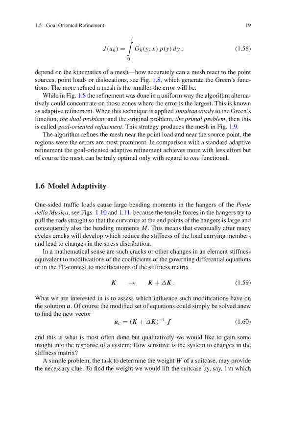
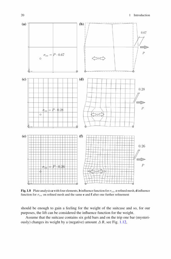
depend on the kinematics of a mesh—how accurately can a mesh react to the pointsources, point loads or dislocations, see Fig. 1.8, which generate the Green’s func-tions. The more refined a mesh is the smaller the error will be.

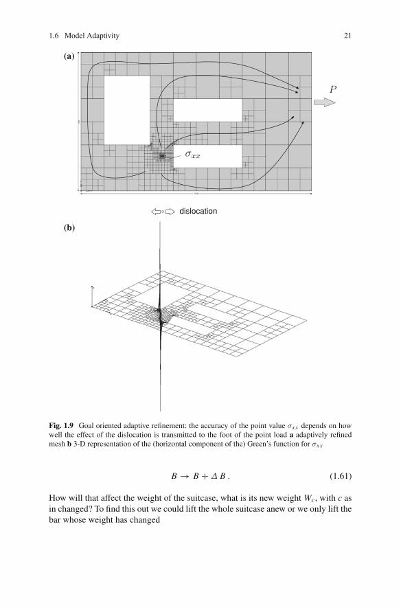
While in Fig. 1.8 the refinement was done in a uniform way the algorithm alterna-tively could concentrate on those zones where the error is the largest. This is knownas adaptive refinement. When this technique is applied simultaneously to the Green’sfunction, the dual problem, and the original problem, the primal problem, then thisis called goal-oriented refinement. This strategy produces the mesh in Fig. 1.9.

The algorithm refines the mesh near the point load and near the source point, theregions were the errors are most prominent. In comparison with a standard adaptiverefinement the goal-oriented adaptive refinement achieves more with less effort butof course the mesh can be truly optimal only with regard to one functional.

1.6 Model Adaptivity

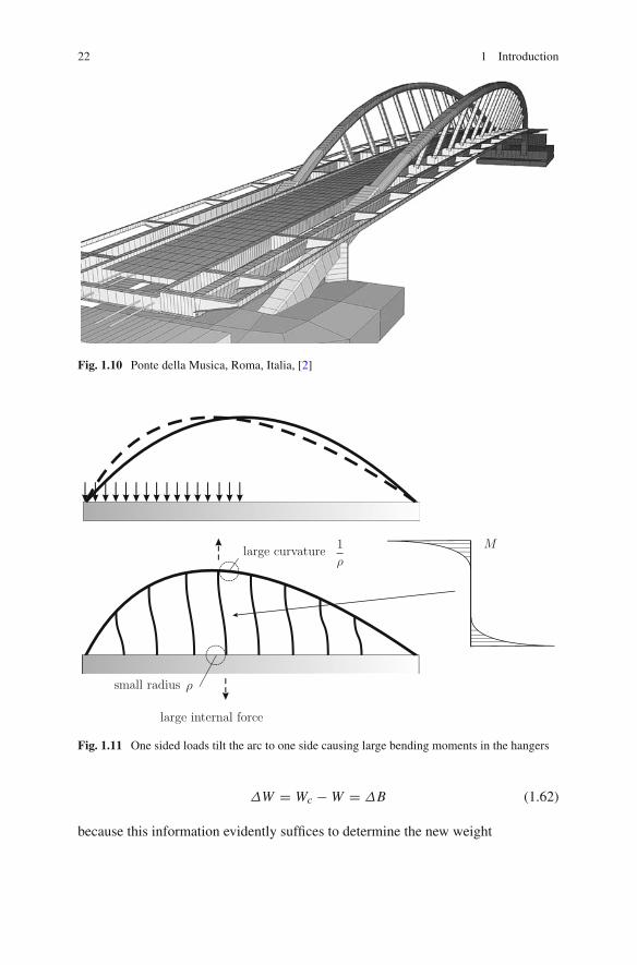
One-sided traffic loads cause large bending moments in the hangers of the Pontedella Musica, see Figs. 1.10 and 1.11, because the tensile forces in the hangers try topull the rods straight so that the curvature at the end points of the hangers is large andconsequently also the bending moments M . This means that eventually after manycycles cracks will develop which reduce the stiffness of the load carrying membersand lead to changes in the stress distribution.

In a mathematical sense are such cracks or other changes in an element stiffnessequivalent to modifications of the coefficients of the governing differential equationsor in the FE-context to modifications of the stiffness matrix

K → K +ΔK . (1.59)

What we are interested in is to assess which influence such modifications have onthe solution u. Of course the modified set of equations could simply be solved anewto find the new vector

uc = (K +ΔK )−1 f (1.60)

and this is what is most often done but qualitatively we would like to gain someinsight into the response of a system: How sensitive is the system to changes in thestiffness matrix?

A simple problem, the task to determine the weight W of a suitcase, may providethe necessary clue. To find the weight we would lift the suitcase by, say, 1 m which

20 1 Introduction

(a) (b)

(c) (d)

(f)(e)

Fig. 1.8 Plate analysis a with four elements, b influence function forσxx , c refined mesh, d influencefunction for σxx on refined mesh and the same e and f after one further refinement

should be enough to gain a feeling for the weight of the suitcase and so, for ourpurposes, the lift can be considered the influence function for the weight.

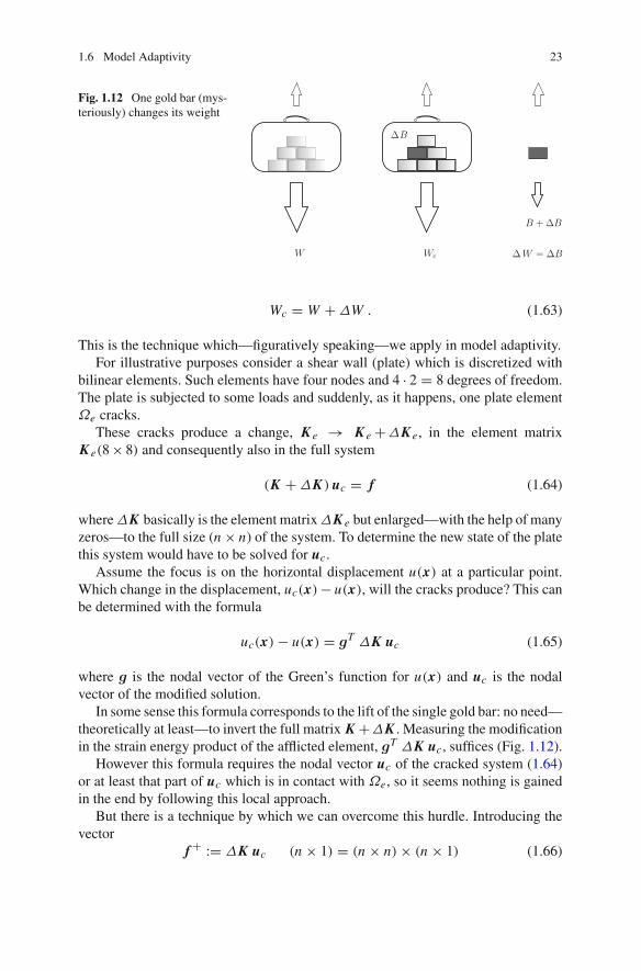
Assume that the suitcase contains six gold bars and on the trip one bar (mysteri-ously) changes its weight by a (negative) amount Δ B, see Fig. 1.12,

1.6 Model Adaptivity 21

dislocation

(a)

(b)

Fig. 1.9 Goal oriented adaptive refinement: the accuracy of the point value σxx depends on howwell the effect of the dislocation is transmitted to the foot of the point load a adaptively refinedmesh b 3-D representation of the (horizontal component of the) Green’s function for σxx

B → B +Δ B . (1.61)

How will that affect the weight of the suitcase, what is its new weight Wc, with c asin changed? To find this out we could lift the whole suitcase anew or we only lift thebar whose weight has changed

22 1 Introduction

Fig. 1.10 Ponte della Musica, Roma, Italia, [2]

Fig. 1.11 One sided loads tilt the arc to one side causing large bending moments in the hangers

ΔW = Wc −W = ΔB (1.62)

because this information evidently suffices to determine the new weight

1.6 Model Adaptivity 23

Fig. 1.12 One gold bar (mys-teriously) changes its weight

Wc = W +ΔW . (1.63)

This is the technique which—figuratively speaking—we apply in model adaptivity.For illustrative purposes consider a shear wall (plate) which is discretized with

bilinear elements. Such elements have four nodes and 4 · 2 = 8 degrees of freedom.The plate is subjected to some loads and suddenly, as it happens, one plate elementΩe cracks.

These cracks produce a change, K e → K e+ΔK e, in the element matrixK e(8× 8) and consequently also in the full system

(K +ΔK ) uc = f (1.64)

where ΔK basically is the element matrix ΔK e but enlarged—with the help of manyzeros—to the full size (n× n) of the system. To determine the new state of the platethis system would have to be solved for uc.

Assume the focus is on the horizontal displacement u(x) at a particular point.Which change in the displacement, uc(x)− u(x), will the cracks produce? This canbe determined with the formula

uc(x)− u(x) = gT ΔK uc (1.65)

where g is the nodal vector of the Green’s function for u(x) and uc is the nodalvector of the modified solution.

In some sense this formula corresponds to the lift of the single gold bar: no need—theoretically at least—to invert the full matrix K +ΔK . Measuring the modificationin the strain energy product of the afflicted element, gT ΔK uc, suffices (Fig. 1.12).

However this formula requires the nodal vector uc of the cracked system (1.64)or at least that part of uc which is in contact with Ωe, so it seems nothing is gainedin the end by following this local approach.

But there is a technique by which we can overcome this hurdle. Introducing thevector

f+ := ΔK uc (n × 1) = (n × n)× (n × 1) (1.66)

24 1 Introduction

the equation takes the form

uc(x)− u(x) = gT f+ (1× n) (n × 1) . (1.67)

This vector

f+ = {0, 0, . . . , 0, ∗, ∗, ∗, ∗, ∗, ∗, ∗, ∗︸ ︷︷ ︸f+e

, 0, . . . , 0, 0}T (1.68)

has only eight non-zero entries because the matrix ΔK is essentially the 8× 8 elementmatrix ΔK e and not much else and so only those parts of the vectors g and uc whichare in contact with the defective element Ωe enter the equation

uc(x)− u(x) = gTe f+e (1× 8) (8× 1) . (1.69)

Here ge and f+e designate the parts of g and f which have contact with Ωe.As will be shown later f+e can be determined by solving a small system of size

8× 8(Fe +ΔK−1

e ) f+e = ue (1.70)

where ue(8 × 1) are the nodal displacements of the element �e before the cracksdeveloped. The matrix Fe is the local part, (8 × 8), of the flexibility matrix ofthe system, that is the inverse K−1 of the full system matrix; for details, how the(normally) singular element matrix ΔK e can be inverted and how the entries of Fe

can be found without calculating the inverse K−1, see Chap. 5.Adding the vector f+ to the right-hand side of the original equation

K uc = f + f+ (1.71)

produces the vector uc, the displacement vector of the cracked system! This implies—and this is the important part—that the Green’s function of the uncracked system(vector g) allows to predict the displacements (and all other observables as well) ofthe cracked system

uc(x) = gT ( f + f+) . (1.72)

Whether this approach has any advantage over the “brute force” approach wherethe modified system (K + ΔK ) uc = f is simply solved for uc depends on thecircumstances.

But irrespective of the computational merits of the equation

uc(x)− u(x) = gT ΔK uc (1.73)

1.6 Model Adaptivity 25

(a)

(b)

(c)

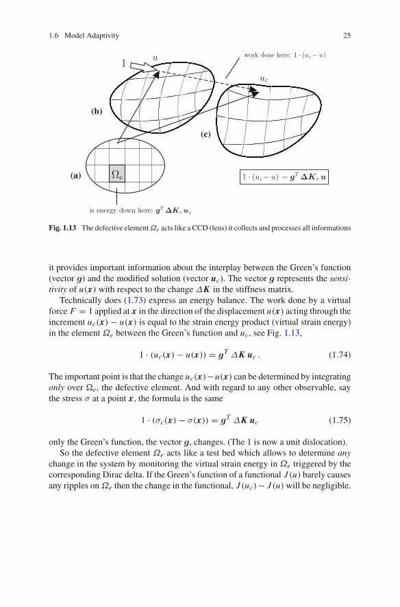
Fig. 1.13 The defective element Ωe acts like a CCD (lens) it collects and processes all informations

it provides important information about the interplay between the Green’s function(vector g) and the modified solution (vector uc). The vector g represents the sensi-tivity of u(x) with respect to the change ΔK in the stiffness matrix.

Technically does (1.73) express an energy balance. The work done by a virtualforce F = 1 applied at x in the direction of the displacement u(x) acting through theincrement uc(x)− u(x) is equal to the strain energy product (virtual strain energy)in the element Ωe between the Green’s function and uc, see Fig. 1.13,

1 · (uc(x)− u(x)) = gT ΔK uc . (1.74)

The important point is that the change uc(x)−u(x) can be determined by integratingonly over �e, the defective element. And with regard to any other observable, saythe stress σ at a point x, the formula is the same

1 · (σc(x)− σ(x)) = gT ΔK uc (1.75)

only the Green’s function, the vector g, changes. (The 1 is now a unit dislocation).So the defective element Ωe acts like a test bed which allows to determine any

change in the system by monitoring the virtual strain energy in Ωe triggered by thecorresponding Dirac delta. If the Green’s function of a functional J (u) barely causesany ripples on Ωe then the change in the functional, J (uc)− J (u) will be negligible.

26 1 Introduction

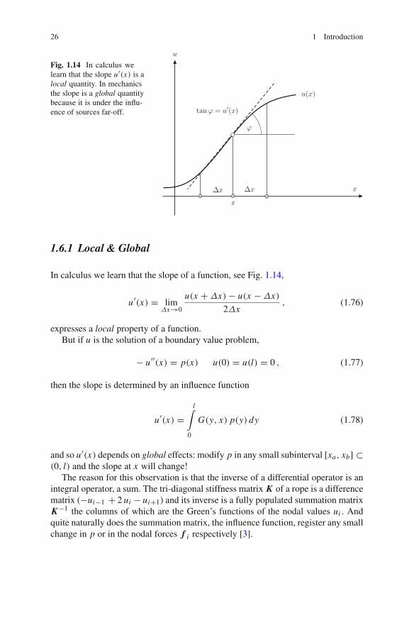
Fig. 1.14 In calculus welearn that the slope u′(x) is alocal quantity. In mechanicsthe slope is a global quantitybecause it is under the influ-ence of sources far-off.

1.6.1 Local & Global

In calculus we learn that the slope of a function, see Fig. 1.14,

u′(x) = limΔx→0

u(x +Δx)− u(x −Δx)

2Δx, (1.76)

expresses a local property of a function.But if u is the solution of a boundary value problem,

− u′′(x) = p(x) u(0) = u(l) = 0 , (1.77)

then the slope is determined by an influence function

u′(x) =l∫

0

G(y, x) p(y) dy (1.78)

and so u′(x) depends on global effects: modify p in any small subinterval [xa, xb] ⊂(0, l) and the slope at x will change!

The reason for this observation is that the inverse of a differential operator is anintegral operator, a sum. The tri-diagonal stiffness matrix K of a rope is a differencematrix (−ui−1 + 2 ui − ui+1) and its inverse is a fully populated summation matrixK−1 the columns of which are the Green’s functions of the nodal values ui . Andquite naturally does the summation matrix, the influence function, register any smallchange in p or in the nodal forces f i respectively [3].

1.7 How to Calculate Influence Functions with Finite Elements 27

1.7 How to Calculate Influence Functionswith Finite Elements

Influence functions are displacements, they have nodal values ui as ordinary functionsdo and these nodal values are the solution of the system K u = f just as in standardFE-analysis. The only question is: which nodal forces fi (or ji as we usually callthem) do generate the influence functions?

Two examples may suffice to give the idea. (1) The equivalent nodal forces fi

which generate the influence function for the value u(x) of the solution at a point xare the values of the shape functions at this point x

fi = ϕi (x) . (1.79)

(2) The forces fi which generate the influence function for the stress σ(x) at a pointx are the stresses

fi = σ(ϕi )(x) (1.80)

of the shape functions at the point x—and so on. So the rule is easy:

Theorem 1.2 (Nodal forces for influence functions) The Green’s function for alinear functional J (u) is generated by applying the values fi = J (ϕi ) of the shapefunctions ϕi as equivalent nodal forces

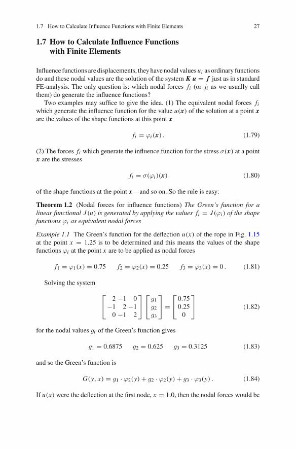
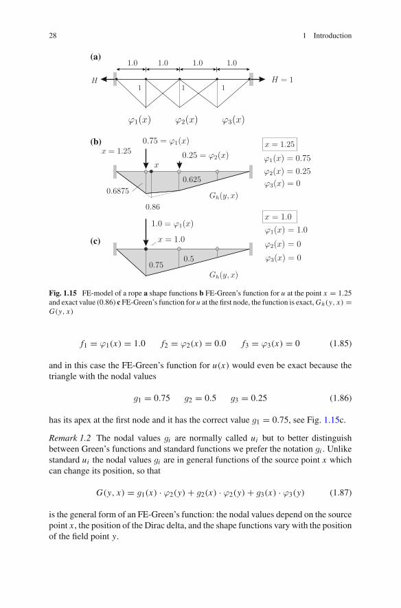
Example 1.1 The Green’s function for the deflection u(x) of the rope in Fig. 1.15at the point x = 1.25 is to be determined and this means the values of the shapefunctions ϕi at the point x are to be applied as nodal forces

f1 = ϕ1(x) = 0.75 f2 = ϕ2(x) = 0.25 f3 = ϕ3(x) = 0 . (1.81)

Solving the system

⎡⎣ 2 −1 0−1 2 −1

0 −1 2

⎤⎦

⎡⎣ g1g2g3

⎤⎦ =

⎡⎣ 0.75

0.250

⎤⎦ (1.82)

for the nodal values gi of the Green’s function gives

g1 = 0.6875 g2 = 0.625 g3 = 0.3125 (1.83)

and so the Green’s function is

G(y, x) = g1 · ϕ2(y)+ g2 · ϕ2(y)+ g3 · ϕ3(y) . (1.84)

If u(x) were the deflection at the first node, x = 1.0, then the nodal forces would be

28 1 Introduction

(a)

(b)

(c)

Fig. 1.15 FE-model of a rope a shape functions b FE-Green’s function for u at the point x = 1.25and exact value (0.86) c FE-Green’s function for u at the first node, the function is exact, Gh(y, x) =G(y, x)

f1 = ϕ1(x) = 1.0 f2 = ϕ2(x) = 0.0 f3 = ϕ3(x) = 0 (1.85)

and in this case the FE-Green’s function for u(x) would even be exact because thetriangle with the nodal values

g1 = 0.75 g2 = 0.5 g3 = 0.25 (1.86)

has its apex at the first node and it has the correct value g1 = 0.75, see Fig. 1.15c.

Remark 1.2 The nodal values gi are normally called ui but to better distinguishbetween Green’s functions and standard functions we prefer the notation gi . Unlikestandard ui the nodal values gi are in general functions of the source point x whichcan change its position, so that

G(y, x) = g1(x) · ϕ2(y)+ g2(x) · ϕ2(y)+ g3(x) · ϕ3(y) (1.87)

is the general form of an FE-Green’s function: the nodal values depend on the sourcepoint x , the position of the Dirac delta, and the shape functions vary with the positionof the field point y.

1.7 How to Calculate Influence Functions with Finite Elements 29

In some books the source point is denoted by the Greek letter ξ, allowing the x tobe the field variable, but that would make the solution u to be a function of ξ whenthe influence function is evaluated

u(ξ) =l∫

0

G(x, ξ) p(x) dx . (1.88)

This is the reason why we prefer the combination x and y.

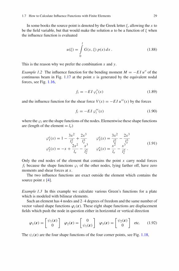
Example 1.2 The influence function for the bending moment M = −E I u′′ of thecontinuous beam in Fig. 1.17 at the point x is generated by the equivalent nodalforces, see Fig. 1.16,

fi = −E I ϕ′′i (x) (1.89)

and the influence function for the shear force V (x) = −E I u′′′(x) by the forces

fi = −E I ϕ′′′i (x) (1.90)

where theϕi are the shape functions of the nodes. Elementwise these shape functionsare (length of the element = le)

ϕe1(x) = 1− 3x2

l2e+ 2x3

l3e

ϕe2(x) = −x + 2x2

le− x3

l2e

ϕe3(x) = 3x2

l2e− 2x3

l3e

ϕe4(x) = x2

le− x3

l2e

.

(1.91)

Only the end nodes of the element that contains the point x carry nodal forcesfi because the shape functions ϕi of the other nodes, lying farther off, have zeromoments and shear forces at x .

The two influence functions are exact outside the element which contains thesource point x [4].

Example 1.3 In this example we calculate various Green’s functions for a platewhich is modeled with bilinear elements.

Such an element has 4 nodes and 2 ·4 degrees of freedom and the same number ofvector valued shape functions ϕi (x). These eight shape functions are displacementfields which push the node in question either in horizontal or vertical direction

ϕ1(x) =[ψ1(x)

0

]ϕ2(x) =

[0

ψ1(x)

]ϕ3(x) =

[ψ2(x)

0

]etc. (1.92)

The ψi (x) are the four shape functions of the four corner points, see Fig. 1.18,

30 1 Introduction

Fig. 1.16 Beam element a the four shape functions ϕi and b the corresponding bending momentsM and c shear forces V . The values at the quarter point x = 0.25 l are the nodal forces fi whichgenerate the influence functions for M and V respectively in the next figure

(a)

(b)

Fig. 1.17 FE-Green’s function for a the bending moment M and b the shear force V at the point x

ψ1(x) = 1

4 a b(a − 2x)(b − 2y) ψ2(x) = 1

4 a b(a + 2x)(b − 2y)

(1.93)

ψ3(x) = 1

4 a b(a + 2x)(b + 2y) ψ4(x) = 1

4 a b(a − 2x)(b + 2y) .

(1.94)

1.7 How to Calculate Influence Functions with Finite Elements 31

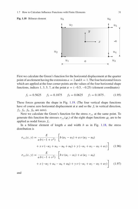
Fig. 1.18 Bilinear element

First we calculate the Green’s function for the horizontal displacement at the quarterpoint of an element having the extensions a = 2 and b = 1. The four horizontal forceswhich are applied at the four corner points are the values of the four horizontal shapefunctions, indices 1, 3, 5, 7, at the point x = (−0.5,−0.25) (element coordinates)

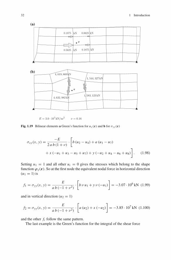
f1 = 0.5625 f3 = 0.1875 f5 = 0.0625 f7 = 0.1875 . (1.95)

These forces generate the shape in Fig. 1.19. (The four vertical shape functionshave of course zero horizontal displacement at x and so the fi in vertical direction,f2, f4, f6, f8, are zero).

Next we calculate the Green’s function for the stress σyy at the same point. Togenerate this function the stresses σyy(ϕi ) of the eight shape functions ϕi are to beapplied as nodal forces fi .

In a bilinear element of length a and width b as in Fig. 1.18, the stressdistribution is

σxx (x, y) = E

a b (−1+ ν2)·[

b (u1 − u3)+ a ν (u2 − u8)

+ x ν (−u2 + u4 − u6 + u8)+ y (−u1 + u3 − u5 + u7)

](1.96)

σyy(x, y) = E

a b (−1+ ν2)·[

b ν (u1 − u3)+ a (u2 − u8)

+ x (−u2 + u4 − u6 + u8)+ y ν (−u1 + u3 − u5 + u7)

](1.97)

and

32 1 Introduction

(a)

(b)

Fig. 1.19 Bilinear elements a Green’s function for ux (x) and b for σyy(x)

σxy(x, y) = −E

2 a b (1+ ν) ·[

b (u2 − u4)+ a (u1 − u7)

+ x (−u1 + u3 − u5 + u7)+ y (−u2 + u4 − u6 + u8)

]. (1.98)

Setting u1 = 1 and all other ui = 0 gives the stresses which belong to the shapefunction ϕ1(x). So at the first node the equivalent nodal force in horizontal direction(u1 = 1) is

f1 = σyy(x, y) = E

a b (−1+ ν2)·[

b ν u1+ y ν (−u1)

]= −3.07 · 106 kN (1.99)

and in vertical direction (u2 = 1)

f2 = σyy(x, y) = E

a b (−1+ ν2)·[

a (u2)+ x (−u2)

]= −3.85 · 107 kN (1.100)

and the other fi follow the same pattern.The last example is the Green’s function for the integral of the shear force

1.7 How to Calculate Influence Functions with Finite Elements 33

(a)

(b)

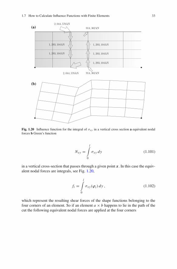
Fig. 1.20 Influence function for the integral of σxy in a vertical cross section a equivalent nodalforces b Green’s function

Nxy =l∫

0

σxy dy (1.101)

in a vertical cross-section that passes through a given point x. In this case the equiv-alent nodal forces are integrals, see Fig. 1.20,

fi =l∫

0

σxy(ϕi ) dy , (1.102)

which represent the resulting shear forces of the shape functions belonging to thefour corners of an element. So if an element a × b happens to lie in the path of thecut the following equivalent nodal forces are applied at the four corners

34 1 Introduction

f ei =

b∫0

σxy(ϕi ) dy = −E

2 a (1+ ν) ·[

b (u2 − u4)+ a (u1 − u7)

+ x (−u1 + u3 − u5 + u7)+ b

2(−u2 + u4 − u6 + u8)

](1.103)

where x is the x-coordinate of the cut.For f e

1 set u1 = 1 and all other ui = 0. For f e2 set u2 = 1 and all other ui = 0, etc.

The notation f ei is to indicate that these are element forces, element contributions.

The total nodal force fi is the sum of the single element contributions to a node.

References

1. James DL (2001) Multiresolution green’s function methods for interactive simulations of large-scale elastostatic objects and other physical systems in equilibrium, Ph.D. Thesis, Inst ApplMath, University of British Columbia

2. Ponte della Musica, Roma, Italia, Ing. Giorgio Rizzo, Software: SOFiSTiK3. Strang G (2007) Computational science and engineering. Wellesley-Cambridge Press, Wellesley4. Hartmann F, Katz C (2007) Structural analysis with finite elements. 2nd ed. Springer-Verlag,

Berlin