Greening of the Earth and its drivers - Nature · 1 Greening of the Earth and its drivers 2 Zaichun Zhu 1,2 , Shilong Piao * , Ranga B. Myneni 3 , Mengtian Huang 2 , Zhenzhong 3 Zeng

SUPPLEMENTARY INFORMATIONDOI: 10.1038/NCLIMATE3004

NATURE CLIMATE CHANGE | www.nature.com/natureclimatechange 1

1

Greening of the Earth and its drivers 1

Zaichun Zhu1,2, Shilong Piao1,2*, Ranga B. Myneni3, Mengtian Huang2, Zhenzhong 2

Zeng2, Josep G. Canadell4, Philippe Ciais5,2, Stephen Sitch6, Pierre Friedlingstein7, 3

Almut Arneth8, Chunxiang Cao9, Lei Cheng10, Etsushi Kato11, Charles Koven12, Yue 4

Li2, Xu Lian2, Yongwen Liu2, Ronggao Liu13, Jiafu Mao14, Yaozhong Pan15, Shushi 5

Peng2, Josep Peñuelas16,17, Benjamin Poulter18, Thomas A. M. Pugh8,19, Benjamin D. 6

Stocker20,21, Nicolas Viovy5, Xuhui Wang2, Yingping Wang22, Zhiqiang Xiao23, Hui 7

Yang2, Sönke Zaehle24, Ning Zeng25 8

9

1 Key Laboratory of Alpine Ecology and Biodiversity, Institute of Tibetan Plateau 10

Research, CAS Center for Excellence in Tibetan Plateau Earth Science, Chinese 11

Academy of Sciences, Beijing 100085, China. 12

2 Sino-French Institute for Earth System Science, College of Urban and Environmental 13

Sciences, Peking University, Beijing 100871, China. 14

3 Department of Earth and Environment, Boston University, Boston, Massachusetts 15

02215, USA. 16

4 Global Carbon Project, CSIRO Oceans and Atmosphere, GPO Box 3023, Canberra, 17

ACT 2601, Australia. 18

5 Laboratoire des Sciences du Climat et de l’Environnement (LSCE), CEA CNRS UVSQ, 19

91191 Gif Sur Yvette, France. 20

6 College of Life and Environmental Sciences, University of Exeter, Exeter EX4 4QF, 21

Greening of the Earth and its drivers

© 2016 Macmillan Publishers Limited. All rights reserved.

http://dx.doi.org/10.1038/nclimate3004

2

UK. 1

7 College of Engineering, Mathematics and Physical Sciences, University of Exeter, 2

Exeter EX4 4QF, UK. 3

8 Institute of Meteorology and Climate Research, Atmospheric Environmental Research, 4

Karlsruhe Institute of Technology, 82467 Garmisch-Partenkirchen, Germany. 5

9 State Key Laboratory of Remote Sensing Science, Institute of Remote Sensing and 6

Digital Earth, Chinese Academy of Sciences, Beijing 100101, China. 7

10 CSIRO Land and Water, Black Mountain, Canberra, ACT 2601, Australia. 8

11 Institute of Applied Energy (IAE), Minato-ku, Tokyo 105-0003, Japan. 9

12 Earth Sciences Division, Lawrence Berkeley National Lab, 1 Cyclotron Road, 10

Berkeley, CA 94720, USA. 11

13 LREIS, Institute of Geographic Sciences and Natural Resources Research, Chinese 12

Academy of Sciences, Beijing, 100101, China. 13

14 Climate Change Science Institute and Environmental Sciences Division, Oak Ridge 14

National Laboratory, Oak Ridge, Tennessee 37831, USA. 15

15 College of Resources Science & Technology, State Key Laboratory of Earth 16

Processes and Resource Ecology, Beijing Normal University, Beijing 100875, China. 17

16 CSIC, Global Ecology Unit CREAF-CEAB-UAB, Cerdanyola del Vallès, 08193 18


3

Catalonia, Spain. 1

17 CREAF, Cerdanyola del Vallès, 08193 Catalonia, Spain. 2

18 Montana State University, Institute on Ecosystems and the Department of Ecology, 3

Bozeman, Montana 59717, USA. 4

19 School of Geography, Earth and Environmental Science, University of Birmingham, 5

B15 2TT, UK. 6

20 Department of Life Sciences, Imperial College London, Silwood Park, Ascot, SL5 7

7PY, UK. 8

21 Climate and Environmental Physics, and Oeschger Centre for Climate Change 9

Research, University of Bern, 3012 Bern, Switzerland. 10

22 CSIRO Oceans and Atmosphere, PMB #1, Aspendale, Victoria 3195, Australia. 11

23 State Key Laboratory of Remote Sensing Science, School of Geography, Beijing 12

Normal University, Beijing 100875, China. 13

24 Max-Planck-Institut für Biogeochemie, P.O. Box 600164, Hans-Knöll-Str. 10, 07745 14

Jena, Germany. 15

25 Department of Atmospheric and Oceanic Science, University of Maryland, College 16

Park, MD 20742, USA. 17

*Correspondence to: Shilong Piao, [email protected] 18


4

Supplementary Information 1

2

S1. GIMMS LAI3g 3

The Global Inventory Modeling and Mapping Studies (GIMMS) LAI was 4

generated by an Artificial Neural Network (ANN) model and the third generation 5

AVHRR GIMMS NDVI data set1, 2. The ANN model was first trained with overlapping 6

AVHRR GIMMS NDVI3g data set and best-quality MODIS LAI, and then generate the 7

full temporal coverage GIMMS LAI3g data set using AVHRR GIMMS NDVI3g. The 8

quality and research applicability of GIMMS LAI3g data set were evaluated through 9

direct comparisons with field data and indirectly through inter-comparisons with 10

similar satellite-data products and statistical analysis with climatic variables and 11

ENSO/AO indices1. The GIMMS LAI3g data set, that provides LAI observations at 15-12

day temporal resolution and 1/12 degree spatial resolution for the global vegetation 13

from July 1981 to December 2014, has been widely used in various research purposes3, 14

4, 5, 6. We first composited the 15-day GIMMS LAI3g data to monthly temporal 15

resolution by averaging the two composites in the same month, and then resampled the 16

GIMMS LAI3g data to 0.5° spatial resolution using the bicubic method. 17

S2. GLASS LAI 18

The Global Land Surface Satellite (GLASS) LAI data set was derived from 19

AVHRR, MODIS and CYCLOPES reflectance and LAI products using general 20

regression neural networks7. The GLASS LAI provides global LAI products at 8-day 21

temporal resolution and 1km spatial resolution from 1981 to 2012 in the Integer zed 22

Sinusoidal projection (http://www.bnu-datacenter.com/). The validation against 23

CYCLOPES and MODIS LAI products, as well as field measurements confirms the 24

applicability of GLASS LAI product in long-term study of global vegetation dynamics. 25

We first composited the 8-day GIMMS LAI3g data to monthly temporal resolution by 26

averaging the composites in the same month. Before the averaging process, we 27

weighted each composite by the number of days that the composites fall in the given 28

month. Then, we resampled the GLASS LAI3g data to 0.5° spatial resolution using the 29


http://www.bnu-datacenter.com/

5

bicubic method. 1

S3. GLOBMAP LAI 2

The Global Mapping LAI product was generated by quantitative fusion of MODIS 3

and historical AVHRR data8. The pixel-level relationship between AVHRR and MODIS 4

LAI was first established for the overlapping period 2000-2006 and then used to 5

construct AVHRR LAI back to 1981. The constructed AVHRR LAI and MODIS LAI 6

were combined, which provide a global LAI data set at 15-day temporal resolution and 7

8km spatial resolution for the period 1981 to 2009 8

(http://www.globalmapping.org/globalLAI/). We preprocessed the GLOBMAP LAI 9

using the same method as we used to preprocess the GIMMS LAI3g data set. 10

S4. MEaSUREs FT-ESDR 11

The Freeze/Thaw Earth System Data Record (FT-ESDR) is a NASA Making Earth 12

System Data Records for Use in Research Environments (MEaSUREs) funded effort to 13

provide a consistent daily global data record of land surface freeze/thaw (FT) state 14

dynamics for all vegetated regions that extends 34 years (1979 to 2012)9, 10. The FT-15

ESDR data set was derived from overlapping daily radiometric brightness temperature 16

measurements at 37 GHz frequency from the Scanning Multichannel Microwave 17

Radiometer (SMMR), Special Sensor Microwave Imager (SSM/I) sensor series and the 18

Advanced Microwave Scanning Radiometer for EOS (AMSR-E). 19

S5. Growing season integrated leaf area index 20

The growing season integrated leaf area index (hereafter refer to LAI) has been 21

found to be a good proxy of vegetation primary production11. The growing season 22

duration is evaluated in each vegetated pixel as follows. The Savitzky-Golay filter is 23

first used to smooth the LAI3g data because it maintains the distinctive vegetation time 24

series trajectories and minimizes various atmospheric effects12, 13. The smoothed 15-25

day LAI3g time series is interpolated to daily LAI3g time series using linear 26

interpolation. From the daily LAI3g time series, the LAI-based growing season is 27

determined as: (a) the “start day” is the day when the LAI value is greater than 0.1 and 28


6

has increased by 15% of the amplitude of the growing season; (b) the “end day” is the 1

day when the LAI value is greater than 0.1 and has decreased by 15% of the amplitude 2

of the growing season; (c) the length of growing season is the duration between start 3

day and end day of the growing season. This threshold-based growing season requires 4

refinement in the northern latitudes because the vegetation may remain green during 5

the dormant season due to sub-optimal temperatures and low sunlight levels. The period 6

when the vegetation is actually photosynthetically active is determined by the 7

freeze/thaw state of the ground14, which can be assessed from satellite measurements 8

of passive microwave brightness temperatures10. Fig. S1 shows the global spatial 9

distributions of average start date and duration of growing season for the period 1982 10

to 2009. A comparison of LAI3g integrated over the growing season thus defined with 11

up-scaled flux tower measurements of gross primary production (GPP) showed good 12

correspondence (Fig. S2). This correspondence gives confidence in treating LAI as a 13

proxy for GPP. 14

S6. Uncertainties in satellite observed LAI 15

GIMMS LAI3g, GLASS LAI and GLOBMAP LAI are 3 widely used long-term 16

LAI products that provide global LAI records start from the middle of 1981. These 3 17

LAI data were derived from the legacy AVHRR and MODIS data using different 18

methodologies15. All 3 LAI products have been extensively validated against field 19

measurements and other satellite products, which warrant their suitability of long-term 20

vegetation research. However, we should also pay attention to uncertainties in the 3 21

LAI products. Although all the 3 LAI products consistently show the dominant greening 22

trends over global vegetated area, the spatial distribution and magnitudes of LAI trends 23

are somewhat different (Fig. 1). There are several reasons that may account for the 24

discrepancies and uncertainties in the 3 LAI products. First, the 3 LAI products were 25

generated using different strategies and different AVHRR products1, 7, 8 . Second, the 26

AVHRR sensors lack of on-board calibration and have orbital loss problem, which 27

caused biases that are difficult to be quantified2, 16. Third, although GLASS LAI and 28

GLOBMAP LAI proposed their own methods to merge LAI derived from AVHRR 29


7

sensors and MODIS, it is still difficult to create a consistent LAI time series because 1

AVHRR and MODIS sensors have different spectral characteristics16, 17. These 2

problems are supposed to be solved by generating accurate and consistent LAI time 3

series data in the future. Nevertheless, at present, the 3 LAI products have irreplaceable 4

value to study long-term vegetation research. The 3 LAI data sets were used for 5

detection and attribution of trends in LAI during 1982 to 2009. Specifically, GIMMS 6

LAI3g, the longest remotely sensed LAI data we have, were used to illustrate a 7

continued greening (up to 2014) of global vegetation. 8

S7. Process-based ecosystem models 9

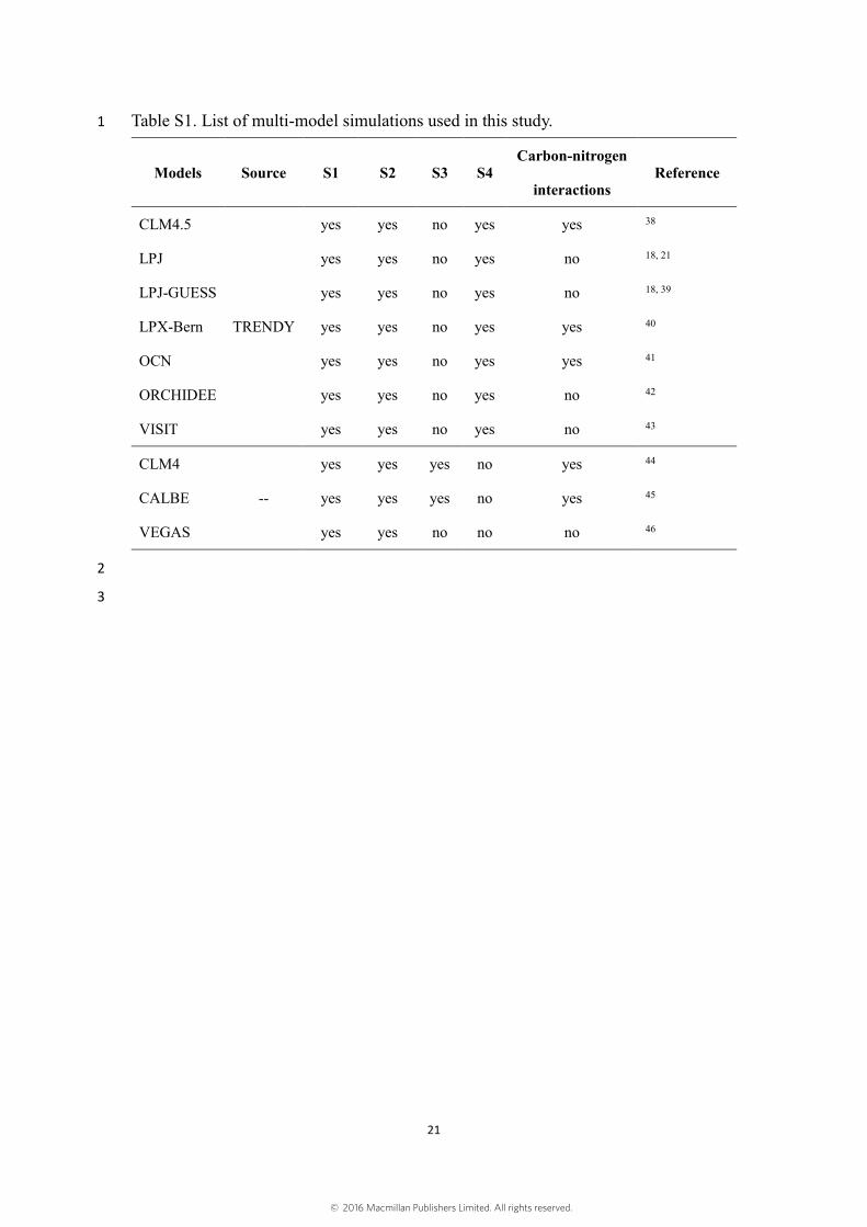
Global monthly LAI for the period 1982 to 2009 simulated by 10 ecosystem 10

models were used in this analysis (Table S1). Seven of the models were coordinated by 11

the project “Trends and drivers of the regional scale sources and sinks of carbon dioxide” 12

(TRENDY, http://dgvm.ceh.ac.uk/node/9)18. Simulations of other 3 models (CLM4, 13

CABLE and VEGAS) were performed under the similar protocol but for the period 14

1982 to 2009. We analyzed data for the period 1982-2009 for which we had access to 15

both satellite observation and outputs from model simulations. All the model outputs 16

were resampled to a common spatial resolution (0.5°) using the nearest neighbor 17

method. 18

The global ecosystem models were forced with historical changes in atmospheric 19

CO2 concentration, climate, nitrogen deposition (in 5 models, Table S1) and land cover 20

change (in 7 models, Table S1). Generally, most ecosystem models that used in our 21

study represented photosynthesis based on Farquhar model. The Farquhar model is a 22

well-established biochemical model that estimates the enzyme kinetics of Rubisco, the 23

main enzyme limiting photosynthesis, based on availability of light, temperature and 24

CO2 concentration in leaf. Although the ecosystem models used similar photosynthesis 25

model, they differ a lot in subcomponents. For example, stomatal conductance model 26

varies between the global ecosystem models. The global ecosystem models represent 27

phenology through the growing degree day (GDD) concept that controlled by 28


http://dgvm.ceh.ac.uk/node/9

8

temperature and soil moisture. However, the parameterizations of their phenology 1

module can differ greatly and affect growing season integrated leaf are index. The Plant 2

Function Type (PFT) is a key concept that allowing for the reduction of thousands of 3

species to a small set of functional groups defined by their phenology type, 4

physiognomy, photosynthetic pathway, and climate zone. PFTs that used by global 5

ecosystem models are sometimes different19. For example, ORCHIDEE defined 12 6

PFTs and used a PFT map that generated by combining simplified Olson biomes with 7

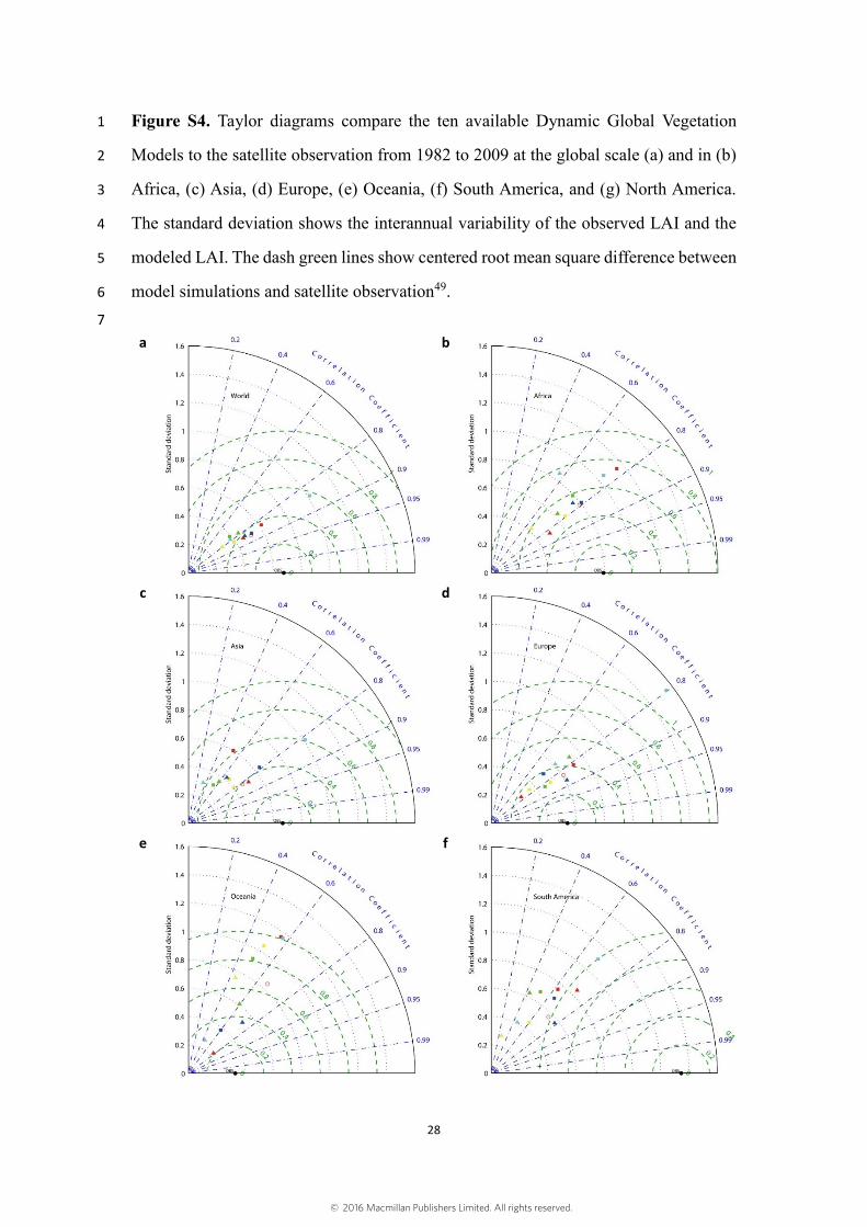
IGBP GLCC data20, while LPJ defined 10 PFTs21. Fig. S4 shows the Taylor diagrams 8

that compare the ten available ecosystem models to the satellite observation from 1982 9

to 2009 at the global scales and continental scales. Fig. S5 shows trends in global 10

averaged LAI derived from individual model simulations driven by rising CO2, climate 11

change, nitrogen deposition and land cover change using Mann-Kendal test. Fig. S6 12

shows the spatial pattern of trends in LAI simulated by individual models under the 13

same scenario S2 (varying CO2 and climate). Both of these figures indicate that there 14

are obvious differences in modeling LAI among the ecosystem models used in our study. 15

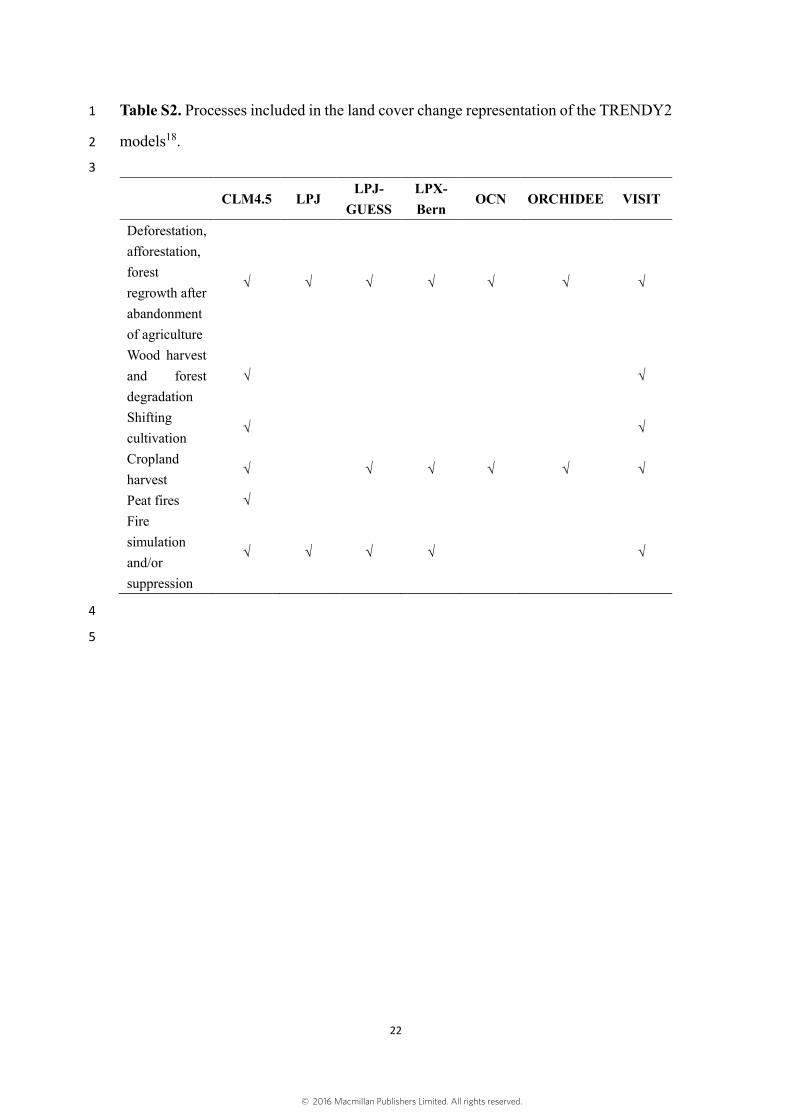
All the 7 global ecosystem models in TRENDY group represent deforestation, 16

afforestation and to some extent regrowth (Table S2) 18. These processes are the most 17

important component of land cover change. The global ecosystem models used a 18

consistent land cover change data22. This land cover change data set not only provides 19

annual fractional data on primary vegetation and secondary vegetation at 0.5 degree 20

spatial resolution, but also underlines transitions between land cover states. Typically, 21

the models only used the information about changes in agricultural areas although the 22

land cover change data also provides the information about changes in the non-23

agricultural areas. The models generally implement this processes differently. For 24

example, an increased cropland fraction in a grid cell can either be at the expense of 25

grassland, or forest (i.e. deforestation)18. 26

All models performed simulations S1 and S2 using global atmospheric CO2 27

concentration23 and historical climate fields from CRU-NCEP data set24. In simulation 28

S1, models were forced with changing atmospheric CO2 concentration, while climate 29


9

was held constant (recycling climate mean and variability from 1901 to 1920). Both 1

atmospheric CO2 concentration and climate were varied in simulation S2. Two models 2

(CLM4 and CABLE) performed an additional simulation (S3) that atmospheric CO2 3

concentration, climate, and nitrogen deposition were all varied. The average difference 4

of S3 and S2 of CLM4 and CABLE was used to assess the relative contribution of 5

nitrogen deposition. The 7 TRENDY models performed an additional scenario that CO2 6

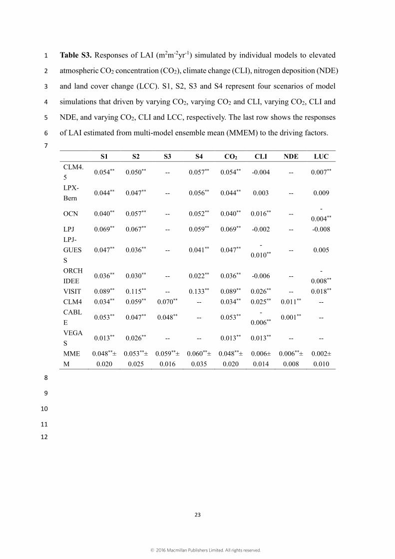
concentration, climate and land-cover were all varied (S4). The difference of S4 and S2 7

were used to evaluate the response of vegetation growth to land use and land cover 8

change. Table S3 lists the responses of LAI that simulated by each individual model to 9

CO2, climate change, nitrogen deposition and land cover change. 10

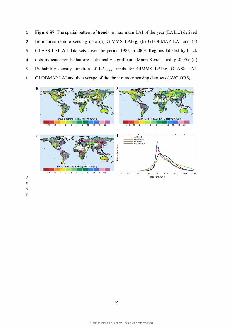
S8. Changes in observed maximum LAI (LAImax) 11

We performed similar trend analyses for the observed LAImax. The results show 12

that LAImax from 3 long-term satellite LAI data sets also consistently show positive 13

trends over a large portion of the global vegetated area during the study period (Figure 14

S7). The patterns of trends in LAImax are similar to that of the trends in growing season 15

LAI. The global greening trend in LAImax estimated from the three data sets is 16

0.012±0.005 m2m-2yr-1. The regions with the largest LAImax greening trends, consistent 17

across the 3 data sets, are in Northern Amazon, Europe, Central Africa and Southeast 18

Asia. The GLASS LAImax data shows the most extensive statistically significant 19

increases (Mann-Kendal test, p<0.05) over 58.6% of vegetated lands, followed by 20

GLOBMAP LAImax (43.5%) and GIMMS LAI3gmax (29.3%). All 3 LAI data sets also 21

consistently show a decreasing LAImax trend over less than 3% of global vegetated land. 22

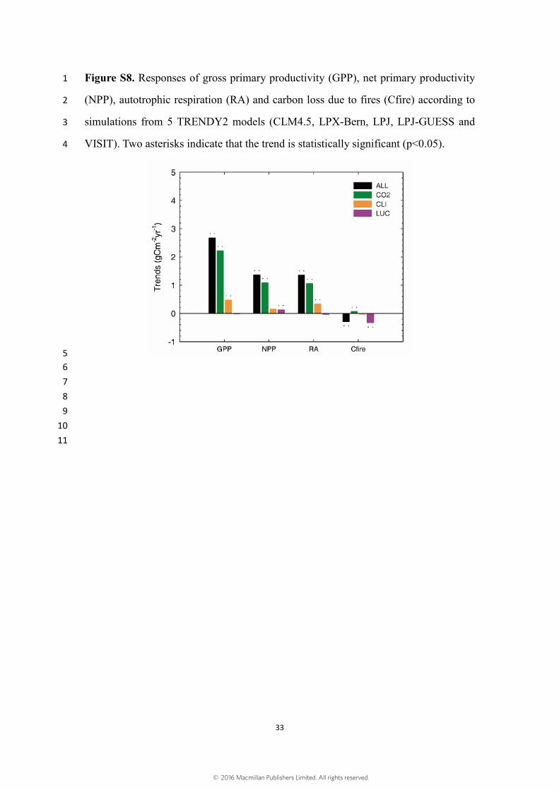
S9. Trends in biosphere parameters that may affect LAI trends 23

Five of the TRENDY2 models (CLM4.5, LPX-Bern, LPJ, LPJ-GUESS and VISIT) 24

provided outputs of gross primary productivity (GPP), net primary productivity (NPP), 25

autotrophic respiration (RA) and carbon emissions due to fires (Cfire). With these 26

outputs, we were able to explore which of these variables exhibit trends related to those 27

of LAI (Fig. S8). According to model simulations, we found that GPP, NPP and RA all 28


10

show statistically significant (p<0.05) increasing trends, while Cfire show statistically 1

significant decreasing trend. The model simulations suggest that increasing GPP, 2

although partly neutralized by increasing RA, and decreasing Cfire are responsible for 3

the increasing LAI during 1982 to 2009. 4

According to model simulations, increases in GPP, NPP and RA and decreases in 5

Cfire due to direct and indirect effects of increasing atmospheric CO2 concentration are 6

all statistically significant (p<0.05). The models also show that increasing atmospheric 7

CO2 concentration contributes the most to increases in GPP, NPP and RA, while LCC 8

effects were the major factor that caused the decrease in Cfire. Climate change 9

statistically significantly stimulated GPP of global vegetation during our study period. 10

However, RA change caused by climate change also statistically significantly increased. 11

These trends almost compensate each other, making the climate-induced change of NPP 12

statistically not significant. The magnitude of Cfire trends is much smaller than trends 13

in GPP, NPP or RA during 1982 to 2009, which suggests that decreasing fires loss was 14

not a major cause of LAI increase. Satellite-based burned area data show that the ratio 15

of global annual burned area to global vegetated area is about 3% and trend in global 16

burned area is about -1% per year 25. Such a small fraction combined with its small 17

trends also suggest the limited role of Satellite-observed burned area data also 18

confirmed the limited role of Cfire in affecting global vegetation. 19

S10. Differences between the spatial pattern of trends in modeled LAI and observed 20

LAI 21

We noticed that the inconsistencies between observations and models are mainly 22

in the Southwestern United States, Southern South American countries, and Mongolia 23

(Fig. 3a and b). In these regions, MMEM suggests that LAI has strongly decreased for 24

the period 1982 to 2009, whereas observation suggests little decreasing or even slightly 25

increasing trends. To investigate the possible reason that caused the differences, we first 26

checked the model fractional simulations. We found that these negative trends were 27

mainly caused by climate change (Fig. S11b). We further investigated which climatic 28


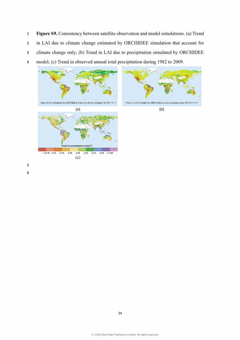
11

factor is most responsible for the negative trends using an additional simulation 1

experiment with ORCHIDEE (Section S13). ORCHIDEE simulation driven by climate 2

change only generally captured the strong negative trends as shown in Fig. S9a. The 3

fractional simulations of ORCHIDEE suggest that trends in precipitation are the 4

dominant driving factor that account for the strong decreasing trends in model-5

simulated LAI (Fig. S9b). We also investigated the global pattern of annual total 6

precipitation using observed precipitation data (CRU). The results show that the (red) 7

regions where simulated LAI decreased in MMEM model simulations match well with 8

the regions where annual total precipitation significantly decreased (Fig. S9c). 9

Such pronounced negative trends were not captured by any of the three satellite 10

products. Our analysis indicated that models may be over-sensitive to trends in 11

precipitation as soil water holding capacities maybe under-estimated in models, and 12

deep rooting, ecosystem composition changes (e.g. shrubification) are not modeled, 13

which is consistent with previous studies26. 14

S11. Optimal Fingerprints Analysis 15

We used an optimal fingerprint method to detect the relative contribution of each 16

external driving factor to the observed change in vegetation activity27, 28. The optimal 17

fingerprint expresses the observation (Y ) as a linear combination of scaled (𝛽𝑖 ) 18

responses to external driving factors (𝑥𝑖 ), which were estimated using ecosystem 19

models, and internal variability (𝜀): 20

Y =∑𝛽𝑖𝑥𝑖 + 𝜀

𝑛

𝑖=1

21

In this study, the LAI simulated by ecosystem models was used to estimate the 22

vegetation change response to external forcing, i.e. CO2 fertilization, climate change, 23

nitrogen deposition and land cover change. Specifically, we used 3 satellite data to 24

calculate the mean LAI. And 10, 10, 2 and 7 simulations (Table S1) were used to 25

calculate the ensemble mean LAI signals driven by CO2 fertilization, climate change, 26

nitrogen deposition and land cover change, respectively. Satellite observed LAI and 27


12

multi-model ensemble mean LAI driven by each external forcing were first aggregated 1

onto global or continental scale and then averaged over 2-year window. The internal 2

variability of changes in vegetation growth was estimated using CMIP5 model control 3

run simulations (Table S4) and preprocessed similar to the signals of external forcings. 4

All the satellite observed LAI and model simulated LAI are centered by subtracting 5

their mean value. We regressed the satellite observed change in LAI onto the multi-6

model ensemble mean LAI driven by CO2 fertilization, climate change, nitrogen 7

deposition and land cover change and estimated their scaling factors using the total least 8

square method28. We also performed similar analysis for the simulated LAI under 9

scenarios S1, S2, S3 and S4. The 95% confidence interval of the estimated scaling 10

factor lies above zero indicates that the signal of the corresponding driving factor is 11

detected. And the corresponding signal is suitable for attribution if the 95% confidence 12

interval contains 1. 13

S12. Analysis of CO2 fertilization effects based on simple concept model 14

The water-use efficiency of photosynthesis is defined as the ratio of the rates of 15

assimilation (A) and transpiration (E) per unit of leaf area29: 16

W =𝐴

𝐸=

𝐶𝑎

1.6𝑣(1 −

𝐶𝑖

𝐶𝑎) (1) 17

where v, Ci and Ca are the leaf-to-air water vapor-pressure deficit and the intercellular 18

and atmospheric CO2 concentrations, respectively. The relative effect of a change in Ca 19

on W is given by: 20

𝑑𝑊

𝑊=

𝑑𝐴

𝐴−

𝑑𝐸

𝐸=

𝑑𝐶𝑎

𝐶𝑎−

𝑑𝑣

𝑣+

𝑑(1−𝐶𝑖𝐶𝑎)

(1−𝐶𝑖𝐶𝑎)

(2) 21

The quantity (1 − 𝐶𝑖 𝐶𝑎⁄ ) has been modeled and observed as being proportional to the 22

square root of the vapor-pressure deficit (√𝑣)30, 31,32. Thus: 23

𝑑𝑊

𝑊=

𝑑𝐴

𝐴−

𝑑𝐸

𝐸=

𝑑𝐶𝑎

𝐶𝑎−

1

2

𝑑𝑣

𝑣 (3) 24

E can be written as: 25


13

E = 1.6𝑔𝑠𝑣 (4) 1

The relative effects of changes in gs and v can be expressed as: 2

𝑑𝐸

𝐸=

𝑑𝑔𝑠

𝑔𝑠+

𝑑𝑣

𝑣 (5) 3

Equation 3 can thus be written as: 4

𝑑𝑊

𝑊=

𝑑𝐴

𝐴−

𝑑𝑔𝑠

𝑔𝑠−

𝑑𝑣

𝑣=

𝑑𝐶𝑎

𝐶𝑎−

1

2

𝑑𝑣

𝑣 (6) 5

and 6

𝑑𝐴

𝐴=

𝑑𝐶𝑎

𝐶𝑎+

1

2

𝑑𝑣

𝑣+

𝑑𝑔𝑠

𝑔𝑠 (7) 7

Atmospheric CO2 concentrations (Ca) increased from 341 to 387 ppm (~46 ppm) 8

during 1982-200933, i.e. 𝑑𝐶𝑎 𝐶𝑎⁄ was 13.5%. We also calculated monthly vapor-9

pressure deficits for the study period using the CRU time-series data 34. The vapor-10

pressure deficit was calculated from the difference between saturated vapor pressure, 11

which was calculated using monthly mean temperature, and the monthly mean vapor-12

pressure data provided by the CRU time series. The results suggested that the relative 13

change of annual mean vapor-pressure deficit over vegetated areas globally (𝑑𝑣 𝑣⁄ ) was 14

about 2.3% for 1982-2009. The experimentally measured response of stomatal 15

conductance to elevated Ca suggested that an increase in Ca of 46 ppm would cause a 16

relative change in stomatal conductance (𝑑𝑔𝑠 𝑔𝑠⁄ ) of -5.0 to -3.0%35, 36. We estimated 17

from equation (7) a relative change of A of about 9.7-11.7% (or 21.1-25.4% per 100 18

ppm). We also estimated from equation (6) a relative change of W of about 12.3%. The 19

results indicated that the direct (𝑑𝐶𝑎 𝐶𝑎⁄ ) and indirect (𝑑𝑔𝑠 𝑔𝑠⁄ ) effects of an increase 20

in Ca were the major factors that affected the change in A during 1982-2009 (8.5-10.5%, 21

or 18.5-22.8% per 100 ppm). 22

We also estimated the relative change of global GPP using the 7 TRENDY2 23

models. The TRENDY2 models suggested that the relative change of GPP during the 24

study period was 5.2-8.3% (11.3-18.0% per 100 ppm), which is comparable to the 25

relative change of GPP estimated by the above simple conceptual leaf-scale model. The 26


14

simulated modeled results were also comparable to the relative changes inferred from 1

the Free-Air CO2 Enrichment (FACE) experiments. The increase in Ca during 1982-2

2009 from the FACE experiment37 led to an increase in NPP of 6.1-9.4% (or 9.5-20.4% 3

per 100 ppm) and an increase in LAI of 0.3-11.1% (or 0.6-24.1% per 100 ppm), and the 4

TRENDY2 models estimated relative increases in global NPP and LAI of 5.2-9.0% (or 5

11.3-19.6% per 100 ppm) and 4.7-9.5% (or 10.2-20.7% per 100 ppm), respectively. Our 6

study, however, referenced few FACE experimental sites, which were mainly in 7

forested regions and thus did not represent the heterogeneity of the CO2 fertilization 8

effects across all representative vegetation types (or model PFTs). 9

The generally comparable relative changes of global vegetation growth estimated 10

from the simple conceptual models, the ecosystem models, and the FACE experiments 11

lend credibility to our estimates of the response of global vegetation to elevated Ca 12

during 1982-2009. Various complex mechanisms control the responses of vegetation 13

growth to Ca, which are (to some extent) represented in our models. Analyzing all these 14

mechanisms from model simulations under predefined scenarios, however, is difficult. 15

The simple conceptual model identified some major mechanisms that control the 16

responses of vegetation to Ca. The theoretical method, however, assumes the absence 17

of other factors such as nutrient limitations or disturbances. Further research on the 18

interactive mechanisms between the CO2 fertilization effects and other factors is needed. 19

S13. Partitioning climate change effects 20

To further understand the response of vegetation trend to climate change, we 21

designed an additional set of scenarios for ORCHIDEE: (ORC_S1) varying 22

atmospheric CO2 concentration and varying climate; (ORC_S2) varying CO2, 23

precipitation and radiation; (ORC_S3) varying CO2, temperature and radiation; 24

(ORC_S4) varying CO2, temperature and precipitation. We accessed the effects of 25

temperature, precipitation and radiation by subtracting ORC_S2, ORC_S3 and 26

ORC_S4 from ORC_S1, respectively. 27

Given that there were large differences in model-simulated responses to changing 28


15

environmental factors, we implemented a two-step analysis to decompose the dominant 1

role of climate change in driving LAI trends. First, we used MMEM to determine the 2

dominant factor that accounts for increasing/decreasing trend in LAI for each vegetated 3

pixel (Fig. 3c). From this analysis, we can determine the pixels where trends (increasing 4

or decreasing) in LAI were dominated by ‘climate change’. Then, we further 5

decomposed ‘climate change’ into climate variables (temperature, precipitation and 6

radiation) in pixels that were dominated by ‘climate change’ using additional specific 7

simulations from ORCHIDEE (Fig. S13). This analysis helped determine the dominant 8

climate variables in the pixels where climate change is the dominant factor as suggested 9

by the MMEM simulations. 10

11


16

References 1

1. Zhu ZC, Bi J, Pan YZ, Ganguly S, Anav A, Xu L, et al. Global data sets of 2

vegetation leaf area index (LAI)3g and fraction of photosynthetically active 3

radiation (FPAR)3g derived from global inventory modeling and mapping studies 4

(GIMMS) normalized difference vegetation index (NDVI3g) for the period 1981 5

to 2011. Remote Sens-Basel 5, 927-948 (2013). 6

2. Pinzon J, Tucker C. A non-stationary 1981–2012 AVHRR NDVI3g time series. 7

Remote Sens-Basel 6, 6929-6960 (2014). 8

3. Anav A, Friedlingstein P, Kidston M, Bopp L, Ciais P, Cox P, et al. Evaluating the 9

land and ocean components of the global carbon cycle in the CMIP5 earth system 10

models. J. Climate 26, 6801-6843 (2013). 11

4. Cook BI, Pau S. A global assessment of long-term greening and browning trends 12

in pasture lands using the GIMMS LAI3g dataset. Remote Sens-Basel 5, 2492-13

2512 (2013). 14

5. Poulter B, Frank D, Ciais P, Myneni RB, Andela N, Bi J, et al. Contribution of 15

semi-arid ecosystems to interannual variability of the global carbon cycle. Nature 16

509, 600-603 (2014). 17

6. Piao S, Nan H, Huntingford C, Ciais P, Friedlingstein P, Sitch S, et al. Evidence 18

for a weakening relationship between interannual temperature variability and 19

northern vegetation activity. Nat. Commun. 5, 5018-5018 (2014). 20

7. Xiao ZQ, Liang SL, Wang JD, Chen P, Yin XJ, Zhang LQ, et al. Use of general 21

regression neural networks for generating the GLASS leaf area index product from 22

time-series modis surface reflectance. IEEE T. Geosci. Remote 52, 209-223 (2014). 23

8. Liu Y, Liu RG, Chen JM. Retrospective retrieval of long-term consistent global 24

leaf area index (1981-2011) from combined AVHRR and MODIS data. J. Geophys. 25

Res. Biogeosci. 117, 440-440 (2012). 26

9. Kim Y, Kimball JS, Zhang K, McDonald KC. Satellite detection of increasing 27

northern hemisphere non-frozen seasons from 1979 to 2008: Implications for 28

regional vegetation growth. Remote Sens. Environ. 121, 472-487 (2012). 29


17

10. Kim Y, Kimball JS, McDonald KC, Glassy J. Developing a global data record of 1

daily landscape freeze/thaw status using satellite passive microwave remote 2

sensing. IEEE T. Geosci. Remote 49, 949-960 (2011). 3

11. Prince SD. Satellite remote-sensing of primary production - comparison of results 4

for sahelian grasslands 1981-1988. Int. J. Remote Sens. 12, 1301-1311 (1991). 5

12. Chen J, Jonsson P, Tamura M, Gu ZH, Matsushita B, Eklundh L. A simple method 6

for reconstructing a high-quality ndvi time-series data set based on the Savitzky-7

Golay filter. Remote Sens. Environ. 91, 332-344 (2004). 8

13. Jonsson P, Eklundh L. Timesat - a program for analyzing time-series of satellite 9

sensor data. Comput. Geosci-UK 30, 833-845 (2004). 10

14. McDonald KC, Kimball JS, Njoku E, Zimmermann R, Zhao MS. Variability in 11

springtime thaw in the terrestrial high latitudes: Monitoring a major control on the 12

biospheric assimilation of atmospheric CO2 with spaceborne microwave remote 13

sensing. Earth Interact. 8, 1-23 (2004). 14

15. Fang H, Jiang C, Li W, Wei S, Baret F, Chen JM, et al. Characterization and 15

intercomparison of global moderate resolution leaf area index (LAI) products: 16

analysis of climatologies and theoretical uncertainties. J. Geophys. Res. Biogeosci. 17

118, 529-548 (2013). 18

16. Tucker CJ, Pinzon JE, Brown ME, Slayback DA, Pak EW, Mahoney R, et al. An 19

extended AVHRR 8-km NDVI dataset compatible with modis and spot vegetation 20

ndvi data. Int. J. Remote Sens. 26, 4485-4498 (2005). 21

17. Guay KC, Beck PSA, Berner LT, Goetz SJ, Baccini A, Buermann W. Vegetation 22

productivity patterns at high northern latitudes: A multi-sensor satellite data 23

assessment. Glob. Change Biol. 20, 3147-3158 (2014). 24

18. Le Quéré C, Peters GP, Andres RJ, Andrew RM, Boden T, Ciais P, et al. Global 25

carbon budget 2013. Earth Syst. Sci. Data Discuss. 6, 689-760 (2013). 26

19. Poulter B, Ciais P, Hodson E, Lischke H, Maignan F, Plummer S, et al. Plant 27

functional type mapping for earth system models. Geosci. Model Dev. 4, 993-1010 28

(2011). 29

20. Krinner G, Viovy N, de Noblet-Ducoudre N, Ogee J, Polcher J, Friedlingstein P, 30


18

et al. A dynamic global vegetation model for studies of the coupled atmosphere-1

biosphere system. Glob. Biogeochem. Cycles 19, GB1015 (2005). 2

21. Sitch S, Smith B, Prentice IC, Arneth A, Bondeau A, Cramer W, et al. Evaluation 3

of ecosystem dynamics, plant geography and terrestrial carbon cycling in the LPJ 4

dynamic global vegetation model. Glob. Change Biol. 9, 161-185 (2003). 5

22. Hurtt GC, Chini LP, Frolking S, Betts RA, Feddema J, Fischer G, et al. 6

Harmonization of land-use scenarios for the period 1500–2100: 600 years of 7

global gridded annual land-use transitions, wood harvest, and resulting secondary 8

lands. Climatic Change, 109, 117-161 (2011). 9

23. Keeling, C. D. & Whorf, T. P. Atmospheric CO2 records from sites in the SIO air 10

sampling network. In Trends: A Compendium of Data on Global Change (Carbon 11

Dioxide Information Analysis Center, Oak Ridge National Laboratory, US DOE, 12

2005) 13

24. New M, Hulme M, Jones P. Representing twentieth-century space-time climate 14

variability. Part ii: Development of 1901-96 monthly grids of terrestrial surface 15

climate. J. Climate, 13, 2217-2238 (2000). 16

25. Giglio L, Randerson JT, van der Werf GR. Analysis of daily, monthly, and annual 17

burned area using the fourth-generation global fire emissions database (GFED4). 18

J. Geophys. Res. Biogeosci. 118, 317-328 (2013). 19

26. Piao SL, Sitch S, Ciais P, Friedlingstein P, Peylin P, Wang XH, et al. Evaluation of 20

terrestrial carbon cycle models for their response to climate variability and to CO2 21

trends. Glob. Change Biol. 19, 2117-2132 (2013). 22

27. Allen MR, Stott PA. Estimating signal amplitudes in optimal fingerprinting, part 23

i: Theory. Clim. Dynam. 21, 477-491 (2003). 24

28. Allen MR, Tett SFB. Checking for model consistency in optimal fingerprinting. 25

Clim. Dynam. 15, 419-434 (1999). 26

29. Wong SC, Cowan IR, Farquhar GD. Stomatal conductance correlates with 27

photosynthetic capacity. Nature 282, 424-426 (1979). 28

30. Farquhar GD, Lloyd J, Taylor JA, Flanagan LB, Syvertsen JP, Hubick KT, et al. 29

Vegetation effects on the isotope composition of oxygen in atmospheric CO2. 30


19

Nature 363, 439-443 (1993). 1

31. Medlyn BE, Duursma RA, Eamus D, Ellsworth DS, Prentice IC, Barton CVM, et 2

al. Reconciling the optimal and empirical approaches to modelling stomatal 3

conductance. Glob. Change Biol. 17, 2134-2144 (2011). 4

32. Donohue RJ, Roderick ML, McVicar TR, Farquhar GD. Impact of CO2 5

fertilization on maximum foliage cover across the globe's warm, arid 6

environments. Geophys. Res. Lett. 40, 3031-3035 (2013). 7

33. Tans P. Trends in atmospheric carbon dioxide. 2015, Available from: 8

www.esrl.noaa.gov/gmd/ccgg/trends/ 9

34. Harris I, Jones PD, Osborn TJ, Lister DH. Updated high-resolution grids of 10

monthly climatic observations - the CRU TS3.10 dataset. Int. J. Climatol. 34, 623-11

642 (2014). 12

35. Ainsworth EA, Rogers A. The response of photosynthesis and stomatal 13

conductance to rising CO2: Mechanisms and environmental interactions. Plant 14

Cell Environ. 30, 258-270 (2007). 15

36. Field CB, Jackson RB, Mooney HA. Stomatal responses to increased CO2 - 16

implications from the plant to the global-scale. Plant Cell Environ. 18, 1214-1225 17

(1995). 18

37. Norby RJ, DeLucia EH, Gielen B, Calfapietra C, Giardina CP, King JS, et al. 19

Forest response to elevated CO2 is conserved across a broad range of productivity. 20

Proc. Natl Acad. Sci. USA 102, 18052-18056 (2005). 21

38. Oleson K, Lawrence DM, Bonan GB, Levis S, Swenson S, Thornton PE, et al. 22

Technical description of version 4.5 of the community land model (CLM); 2013 23

July, 01. Report No. NCAR/TN-503+STR. 24

39. Lindeskog M, Arneth A, Bondeau A, Waha K, Seaquist J, Olin S, et al. 25

Implications of accounting for land use in simulations of ecosystem carbon cycling 26

in africa. Earth Syst. Dynam. 4, 385-407 (2013). 27

40. Stocker BD, Strassmann K, Joos F. Sensitivity of holocene atmospheric CO2 and 28

the modern carbon budget to early human land use: Analyses with a process-based 29

model. Biogeosciences 8, 69-88 (2011). 30


20

41. Zaehle S, Friend AD. Carbon and nitrogen cycle dynamics in the O-CN land 1

surface model: 1. Model description, site-scale evaluation, and sensitivity to 2

parameter estimates. Global Biogeochem. Cycles 24, GB1006 (2010). 3

42. Krinner G, Viovy N, de Noblet-Ducoudré N, Ogée J, Polcher J, Friedlingstein P, 4

et al. A dynamic global vegetation model for studies of the coupled atmosphere-5

biosphere system. Global Biogeochem. Cycles 19, GB1015 (2005). 6

43. Kato E, Kinoshita T, Ito A, Kawamiya M, Yamagata Y. Evaluation of spatially 7

explicit emission scenario of land-use change and biomass burning using a 8

process-based biogeochemical model. J. Land Use Sci. 8, 104-122 (2013). 9

44. Lawrence DM, Oleson KW, Flanner MG, Thornton PE, Swenson SC, Lawrence 10

PJ, et al. Parameterization improvements and functional and structural advances 11

in version 4 of the community land model. J. Adv. Model. Earth Syst. 3, M03001 12

(2011). 13

45. Wang YP, Law RM, Pak B. A global model of carbon, nitrogen and phosphorus 14

cycles for the terrestrial biosphere. Biogeosciences 7, 2261-2282 (2010). 15

46. Zeng N, Neelin JD, Chou C. A quasi-equilibrium tropical circulation model - 16

implementation and simulation. J. Atmos. Sci. 57, 1767-1796 (2000). 17

47. Beer C, Reichstein M, Tomelleri E, Ciais P, Jung M, Carvalhais N, et al. Terrestrial 18

gross carbon dioxide uptake: Global distribution and covariation with climate. 19

Science 329, 834-838 (2010). 20

48. Olson DM, Dinerstein E, Wikramanayake ED, Burgess ND, Powell GVN, 21

Underwood EC, et al. Terrestrial ecoregions of the worlds: A new map of life on 22

earth. Bioscience 51, 933-938 (2001). 23

49. Taylor KE. Summarizing multiple aspects of model performance in a single 24

diagram. J. Geophys. Res. Atmos. 106, 7183-7192 (2001). 25

26

27

28


21

Table S1. List of multi-model simulations used in this study. 1

Models Source S1 S2 S3 S4 Carbon-nitrogen

interactions Reference

CLM4.5

TRENDY

yes yes no yes yes 38

LPJ yes yes no yes no 18, 21

LPJ-GUESS yes yes no yes no 18, 39

LPX-Bern yes yes no yes yes 40

OCN yes yes no yes yes 41

ORCHIDEE yes yes no yes no 42

VISIT yes yes no yes no 43

CLM4

--

yes yes yes no yes 44

CALBE yes yes yes no yes 45

VEGAS yes yes no no no 46

2

3


22

Table S2. Processes included in the land cover change representation of the TRENDY2 1

models18. 2

3

CLM4.5 LPJ

LPJ-

GUESS

LPX-

Bern OCN ORCHIDEE VISIT

Deforestation,

afforestation,

forest

regrowth after

abandonment

of agriculture

√ √ √ √ √ √ √

Wood harvest

and forest

degradation

√ √

Shifting

cultivation √ √

Cropland

harvest √ √ √ √ √ √

Peat fires √

Fire

simulation

and/or

suppression

√ √ √ √ √

4

5


23

Table S3. Responses of LAI (m2m-2yr-1) simulated by individual models to elevated 1

atmospheric CO2 concentration (CO2), climate change (CLI), nitrogen deposition (NDE) 2

and land cover change (LCC). S1, S2, S3 and S4 represent four scenarios of model 3

simulations that driven by varying CO2, varying CO2 and CLI, varying CO2, CLI and 4

NDE, and varying CO2, CLI and LCC, respectively. The last row shows the responses 5

of LAI estimated from multi-model ensemble mean (MMEM) to the driving factors. 6

7

S1 S2 S3 S4 CO2 CLI NDE LUC

CLM4.

5 0.054** 0.050** -- 0.057** 0.054** -0.004 -- 0.007**

LPX-

Bern 0.044** 0.047** -- 0.056** 0.044** 0.003 -- 0.009

OCN 0.040** 0.057** -- 0.052** 0.040** 0.016** -- -

0.004**

LPJ 0.069** 0.067** -- 0.059** 0.069** -0.002 -- -0.008

LPJ-

GUES

S

0.047** 0.036** -- 0.041** 0.047** -

0.010** -- 0.005

ORCH

IDEE 0.036** 0.030** -- 0.022** 0.036** -0.006 --

-

0.008**

VISIT 0.089** 0.115** -- 0.133** 0.089** 0.026** -- 0.018**

CLM4 0.034** 0.059** 0.070** -- 0.034** 0.025** 0.011** --

CABL

E 0.053** 0.047** 0.048** -- 0.053**

-

0.006** 0.001** --

VEGA

S 0.013** 0.026** -- -- 0.013** 0.013** -- --

MME

M

0.048**±

0.020

0.053**±

0.025

0.059**±

0.016

0.060**±

0.035

0.048**±

0.020

0.006±

0.014

0.006**±

0.008

0.002±

0.010

8

9

10

11

12


24

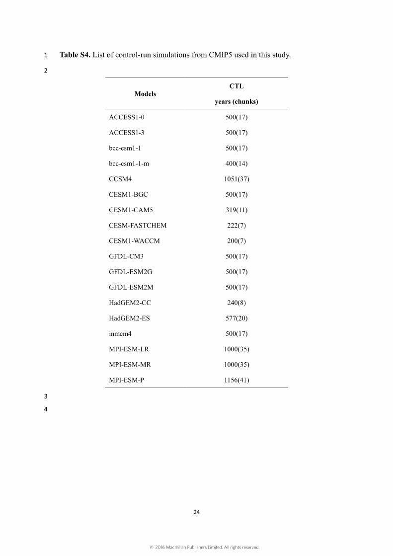
Table S4. List of control-run simulations from CMIP5 used in this study. 1

2

Models CTL

years (chunks)

ACCESS1-0 500(17)

ACCESS1-3 500(17)

bcc-csm1-1 500(17)

bcc-csm1-1-m 400(14)

CCSM4 1051(37)

CESM1-BGC 500(17)

CESM1-CAM5 319(11)

CESM-FASTCHEM 222(7)

CESM1-WACCM 200(7)

GFDL-CM3 500(17)

GFDL-ESM2G 500(17)

GFDL-ESM2M 500(17)

HadGEM2-CC 240(8)

HadGEM2-ES 577(20)

inmcm4 500(17)

MPI-ESM-LR 1000(35)

MPI-ESM-MR 1000(35)

MPI-ESM-P 1156(41)

3

4


25

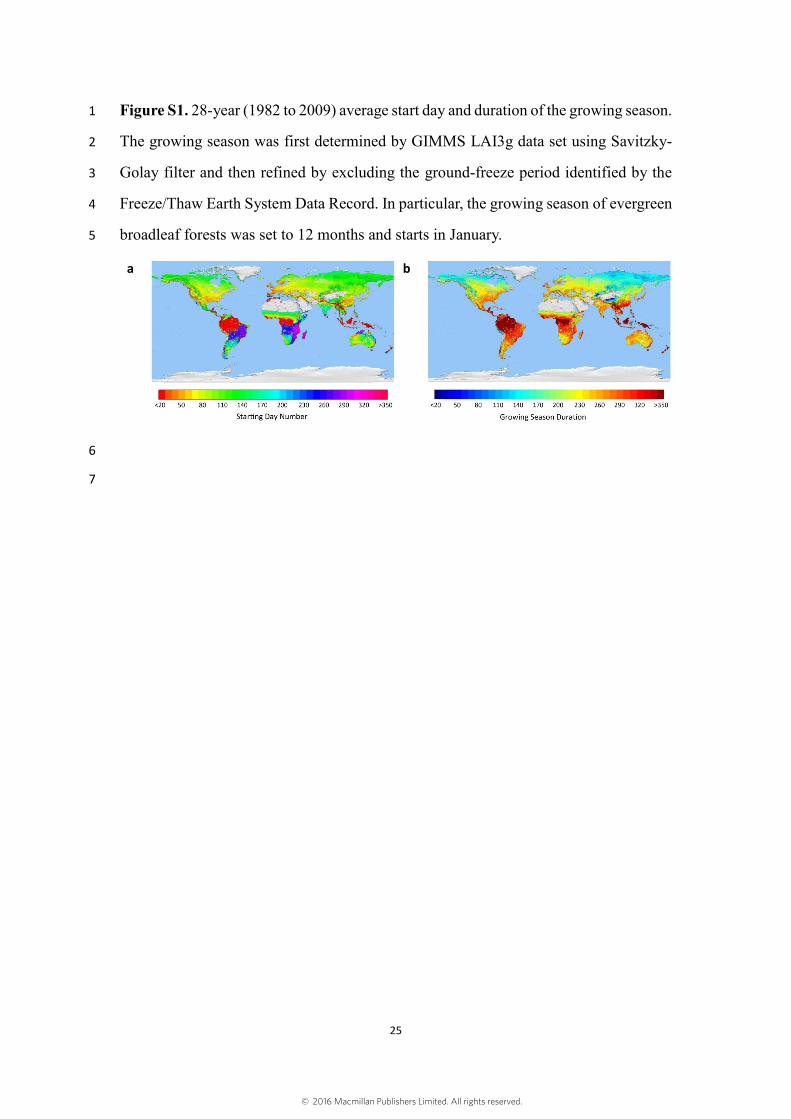
Figure S1. 28-year (1982 to 2009) average start day and duration of the growing season. 1

The growing season was first determined by GIMMS LAI3g data set using Savitzky-2

Golay filter and then refined by excluding the ground-freeze period identified by the 3

Freeze/Thaw Earth System Data Record. In particular, the growing season of evergreen 4

broadleaf forests was set to 12 months and starts in January. 5

a

b

6

7


26

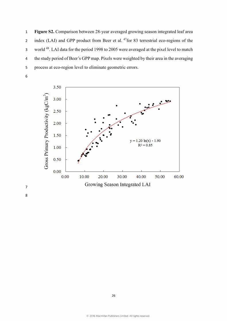
Figure S2. Comparison between 28-year averaged growing season integrated leaf area 1

index (LAI) and GPP product from Beer et al. 47for 83 terrestrial eco-regions of the 2

world 48. LAI data for the period 1998 to 2005 were averaged at the pixel level to match 3

the study period of Beer’s GPP map. Pixels were weighted by their area in the averaging 4

process at eco-region level to eliminate geometric errors. 5

6

7

8


27

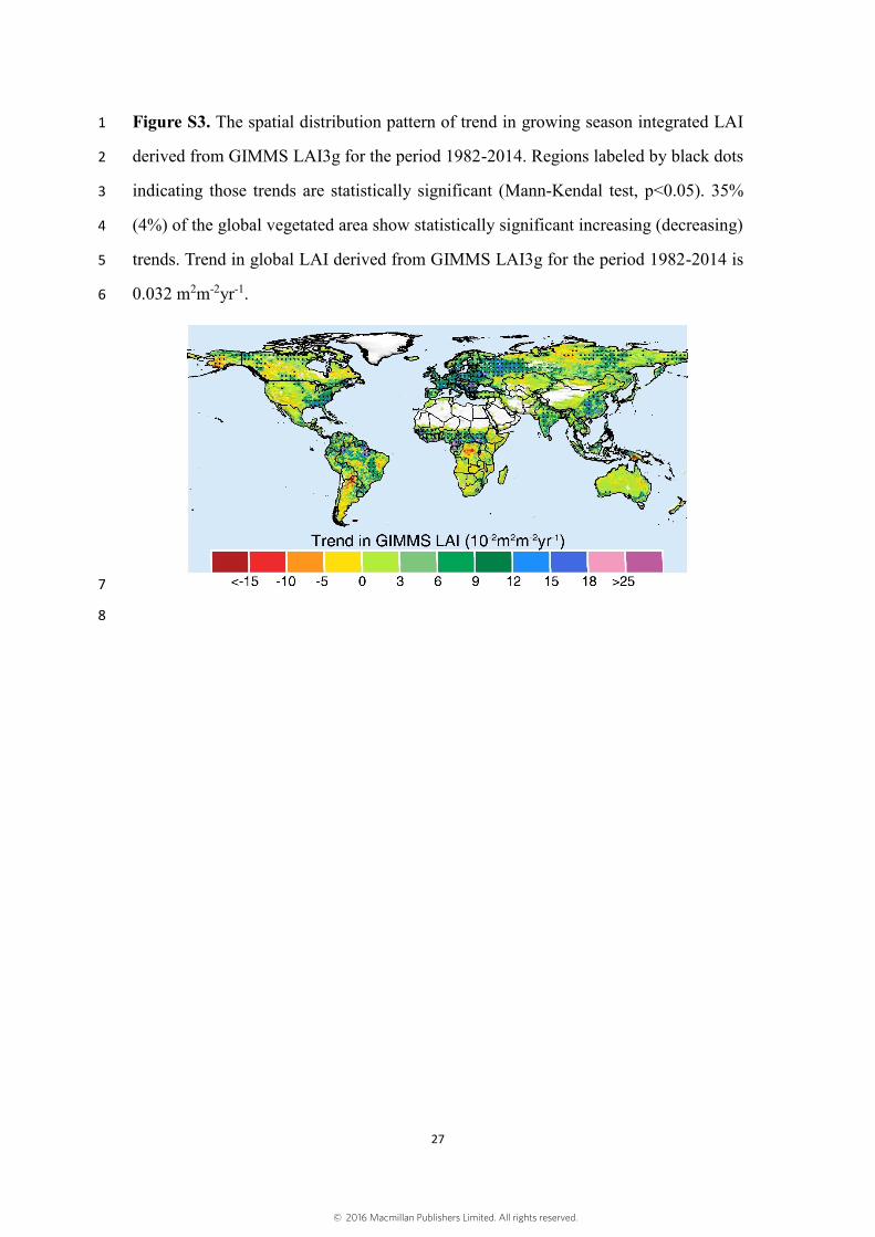
Figure S3. The spatial distribution pattern of trend in growing season integrated LAI 1

derived from GIMMS LAI3g for the period 1982-2014. Regions labeled by black dots 2

indicating those trends are statistically significant (Mann-Kendal test, p<0.05). 35% 3

(4%) of the global vegetated area show statistically significant increasing (decreasing) 4

trends. Trend in global LAI derived from GIMMS LAI3g for the period 1982-2014 is 5

0.032 m2m-2yr-1. 6

7

8


28

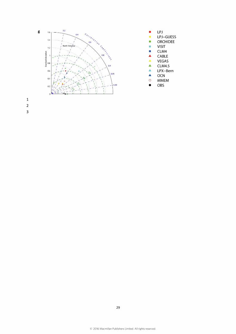
Figure S4. Taylor diagrams compare the ten available Dynamic Global Vegetation 1

Models to the satellite observation from 1982 to 2009 at the global scale (a) and in (b) 2

Africa, (c) Asia, (d) Europe, (e) Oceania, (f) South America, and (g) North America. 3

The standard deviation shows the interannual variability of the observed LAI and the 4

modeled LAI. The dash green lines show centered root mean square difference between 5

model simulations and satellite observation49. 6

7

a

b

c

d

e

f


29

g

1

2

3


30

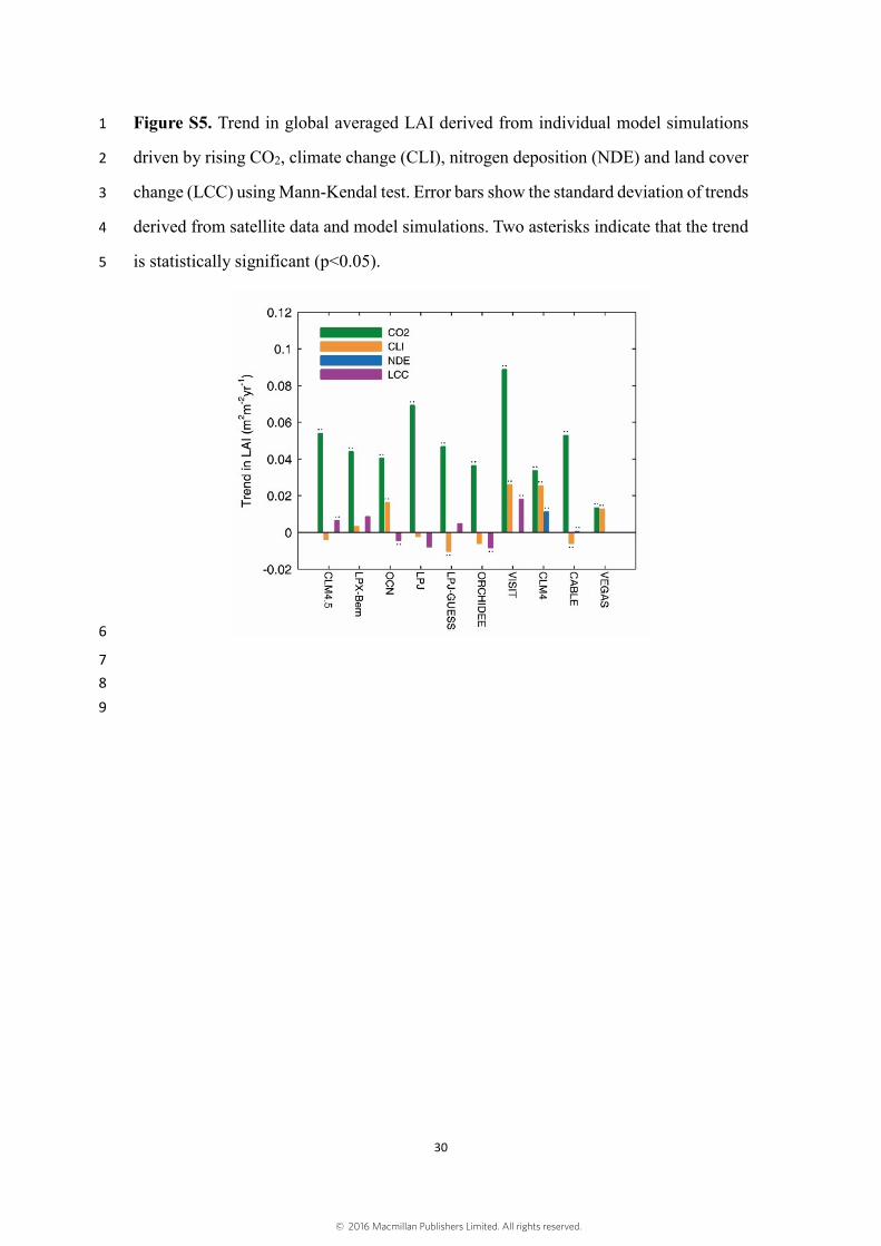
Figure S5. Trend in global averaged LAI derived from individual model simulations 1

driven by rising CO2, climate change (CLI), nitrogen deposition (NDE) and land cover 2

change (LCC) using Mann-Kendal test. Error bars show the standard deviation of trends 3

derived from satellite data and model simulations. Two asterisks indicate that the trend 4

is statistically significant (p<0.05). 5

6

7

8

9


31

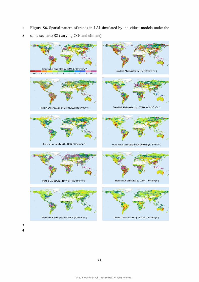
Figure S6. Spatial pattern of trends in LAI simulated by individual models under the 1

same scenario S2 (varying CO2 and climate). 2

3

4


32

Figure S7. The spatial pattern of trends in maximum LAI of the year (LAImax) derived 1

from three remote sensing data (a) GIMMS LAI3g, (b) GLOBMAP LAI and (c) 2

GLASS LAI. All data sets cover the period 1982 to 2009. Regions labeled by black 3

dots indicate trends that are statistically significant (Mann-Kendal test, p<0.05). (d) 4

Probability density function of LAImax trends for GIMMS LAI3g, GLASS LAI, 5

GLOBMAP LAI and the average of the three remote sensing data sets (AVG OBS). 6

7

8

9

10


33

Figure S8. Responses of gross primary productivity (GPP), net primary productivity 1

(NPP), autotrophic respiration (RA) and carbon loss due to fires (Cfire) according to 2

simulations from 5 TRENDY2 models (CLM4.5, LPX-Bern, LPJ, LPJ-GUESS and 3

VISIT). Two asterisks indicate that the trend is statistically significant (p<0.05). 4

5

6

7

8

9

10

11


34

Figure S9. Consistency between satellite observation and model simulations. (a) Trend 1

in LAI due to climate change estimated by ORCHIDEE simulation that account for 2

climate change only; (b) Trend in LAI due to precipitation simulated by ORCHIDEE 3

model; (c) Trend in observed annual total precipitation during 1982 to 2009. 4

(a) (b)

(c)

5

6


35

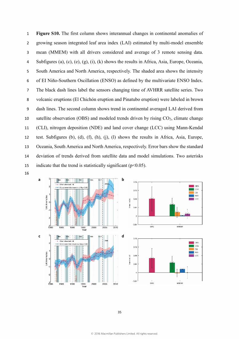
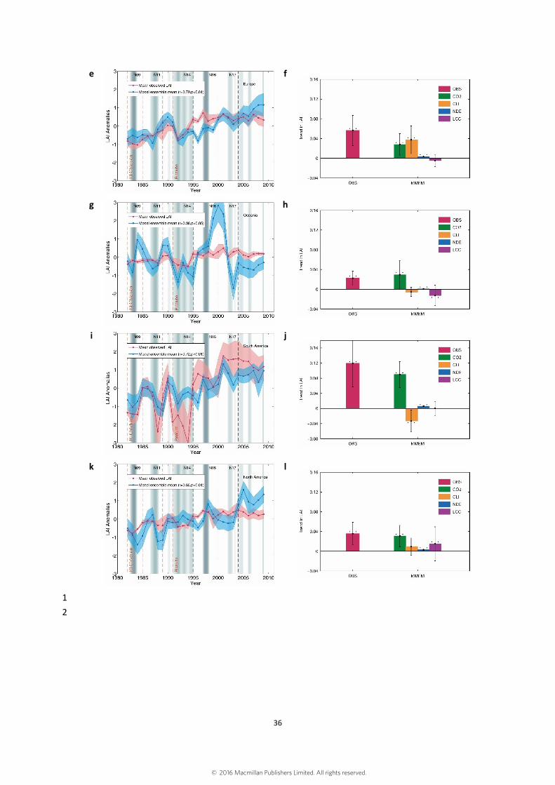
Figure S10. The first column shows interannual changes in continental anomalies of 1

growing season integrated leaf area index (LAI) estimated by multi-model ensemble 2

mean (MMEM) with all drivers considered and average of 3 remote sensing data. 3

Subfigures (a), (c), (e), (g), (i), (k) shows the results in Africa, Asia, Europe, Oceania, 4

South America and North America, respectively. The shaded area shows the intensity 5

of EI Niño-Southern Oscillation (ENSO) as defined by the multivariate ENSO Index. 6

The black dash lines label the sensors changing time of AVHRR satellite series. Two 7

volcanic eruptions (El Chichón eruption and Pinatubo eruption) were labeled in brown 8

dash lines. The second column shows trend in continental averaged LAI derived from 9

satellite observation (OBS) and modeled trends driven by rising CO2, climate change 10

(CLI), nitrogen deposition (NDE) and land cover change (LCC) using Mann-Kendal 11

test. Subfigures (b), (d), (f), (h), (j), (l) shows the results in Africa, Asia, Europe, 12

Oceania, South America and North America, respectively. Error bars show the standard 13

deviation of trends derived from satellite data and model simulations. Two asterisks 14

indicate that the trend is statistically significant (p<0.05). 15

16

a

b

c

d


36

e

f

g

h

i

j

k

l

1

2


37

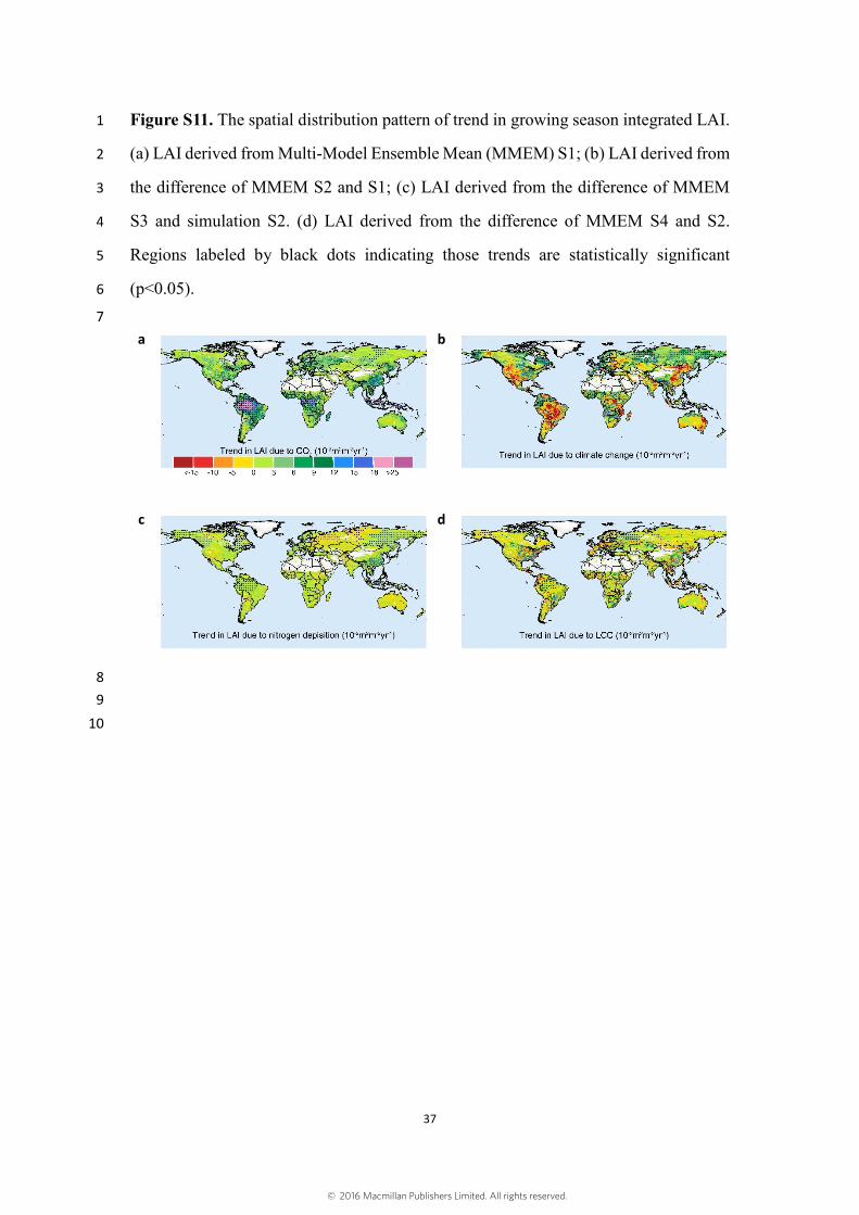
Figure S11. The spatial distribution pattern of trend in growing season integrated LAI. 1

(a) LAI derived from Multi-Model Ensemble Mean (MMEM) S1; (b) LAI derived from 2

the difference of MMEM S2 and S1; (c) LAI derived from the difference of MMEM 3

S3 and simulation S2. (d) LAI derived from the difference of MMEM S4 and S2. 4

Regions labeled by black dots indicating those trends are statistically significant 5

(p<0.05). 6

7

a

b

c

d

8

9

10


38

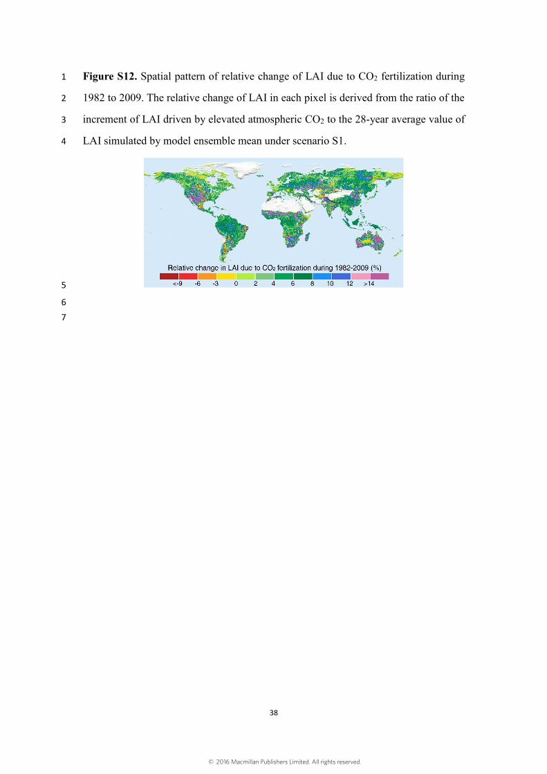
Figure S12. Spatial pattern of relative change of LAI due to CO2 fertilization during 1

1982 to 2009. The relative change of LAI in each pixel is derived from the ratio of the 2

increment of LAI driven by elevated atmospheric CO2 to the 28-year average value of 3

LAI simulated by model ensemble mean under scenario S1. 4

5

6

7


39

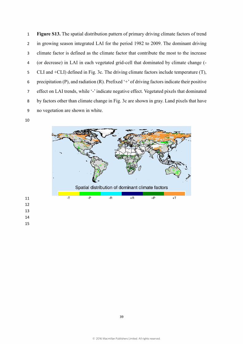
Figure S13. The spatial distribution pattern of primary driving climate factors of trend 1

in growing season integrated LAI for the period 1982 to 2009. The dominant driving 2

climate factor is defined as the climate factor that contribute the most to the increase 3

(or decrease) in LAI in each vegetated grid-cell that dominated by climate change (-4

CLI and +CLI) defined in Fig. 3c. The driving climate factors include temperature (T), 5

precipitation (P), and radiation (R). Prefixed ‘+’ of driving factors indicate their positive 6

effect on LAI trends, while ‘-’ indicate negative effect. Vegetated pixels that dominated 7

by factors other than climate change in Fig. 3c are shown in gray. Land pixels that have 8

no vegetation are shown in white. 9

10

11

12

13

14

15


Documents

Greening of the Earth and its drivers - Nature · 1 Greening of the Earth and its drivers 2 Zaichun Zhu 1,2 , Shilong Piao * , Ranga B. Myneni 3 , Mengtian Huang 2 , Zhenzhong 3 Zeng