Embed Size (px)
Citation preview
DRAFT
December 14, 2010
Greenhouse Gas Emissions Estimation Methodologies for Biogenic Emissions
from Selected Source Categories: Solid Waste Disposal
Wastewater Treatment Ethanol Fermentation
Submitted to:
U.S. Environmental Protection Agency Sector Policies and Programs Division
Measurement Policy Group
Submitted by:
RTI International 3040 Cornwallis Road
Research Triangle Park, NC 27709-2194
EPA Contract No. EP-D-06-118 Work Assignment 4-18
RTI Project Number 0210426.004.018
*RTI International is a Trade Name of Research Triangle Institute

[This page intentionally left blank]
DRAFT GHG Emissions Estimation Methodology for Selected Biogenic Source Categories
iii
Table of Contents Acronyms and Abbreviations ...................................................................................................................... iv
1. Background and Scope ........................................................................................................................ 1-1
2. Solid Waste Disposal ........................................................................................................................... 2-1 2.1 Landfills .................................................................................................................................... 2-1
2.1.1 CH4 Generation ............................................................................................................. 2-2 2.1.2 CO2 Emissions for Landfills without Gas Collection Systems ..................................... 2-5 2.1.3 CO2 Emissions for Landfills with Gas Collection Systems .......................................... 2-6
2.2 Composting Operations .......................................................................................................... 2-11 2.3 Land Treatment Units ............................................................................................................. 2-13
3. Wastewater Treatment ........................................................................................................................ 3-1 3.1 Biological Treatment Processes ................................................................................................ 3-1
3.1.1 Aerobic Treatment Processes ....................................................................................... 3-1 3.1.2 Anaerobic Treatment Processes .................................................................................... 3-2 3.1.3 Facultative Treatment Processes................................................................................... 3-2
3.2 Estimating CH4 and CO2 Emissions ......................................................................................... 3-2 3.2.1 Estimating CH4 and CO2 Emissions from Wastewater and Sludge Treatment
Units ............................................................................................................... 3-4 3.2.2 Estimating CH4 and CO2 Emissions from Combustion of Biogas ............................. 3-10
3.3 Estimating N2O Emissions ..................................................................................................... 3-10
4. Ethanol Fermentation .......................................................................................................................... 4-1 4.1 CO2 Emissions from Sugar- and Starch-based Ethanol Fermentation ..................................... 4-1 4.2 CO2 Emissions from Cellulosic Ethanol Fermentation ............................................................ 4-4 4.3 CO2 Emissions from Direct Measurement Data ....................................................................... 4-5
5. References ........................................................................................................................................... 5-1
List of Figures Figure 3-1. Activated sludge wastewater treatment flow diagram. ........................................................... 3-2 Figure 3-2. Simplified stoichiometric equation for the biochemical oxidation of organic
constituents in wastewater. ...................................................................................................... 3-3 Figure 3-3. Simplified reaction mechanisms for nitrification and denitrification N2O formation. .......... 3-10
List of Tables Table 1-1. Global Warming Potentials for 100-Year Time Horizona ........................................................ 1-3 Table 2-1. Recommended DOC (Degradable Organic Carbon) and Decay Rate Values for
Landfillsa .................................................................................................................................. 2-3 Table 2-2. Additional Landfill Model Defaults ......................................................................................... 2-4 Table 2-3. Default Landfill Gas Collection Efficiencies ........................................................................... 2-8 Table 2-4. Default Emission Factors for Composting ............................................................................. 2-12 Table 3-1. Default Values for Methane Correction Factor and Biomass Yield ......................................... 3-5 Table 3-2. Correction Factors for Equations 3-2 through 3-4 for Different Measurement Method .......... 3-7
DRAFT GHG Emissions Estimation Methodology for Selected Biogenic Source Categories
iv
Acronyms and Abbreviations °R degrees Rankine (= °F + 460) acf actual cubic feet atm atmospheres BACT best available control technology BOD biochemical oxygen demand BOD5 5-day biochemical oxygen demand C carbon CAA Clean Air Act CFR Code of Federal Regulations CH4 methane cm centimeter cBOD carbonaceous biochemical oxygen demand CO carbon monoxide CO2 carbon dioxide CO2e carbon dioxide equivalents COD chemical oxygen demand dscf dry standard cubic feet EPA U.S. Environmental Protection Agency EtOH ethanol FR Federal Register g gram gal gallon Gg gigagram GHG greenhouse gas GWP global warming potential H2 hydrogen H2S hydrogen sulfide IPCC Intergovernmental Panel on Climate Change kg kilogram L liter lb pound m3 cubic meter Mg megagram (= 1 metric ton) mg milligram MLVSS mixed liquor volatile suspended solids mol mole MSW municipal solid waste N2 nitrogen N2O nitrous oxide O2 oxygen POTW publicly owned treatment works PSD Prevention of Significant Deterioration psig pounds per square inch, gauge scf standard cubic feet t short ton Tg teragram (= 106 metric ton) TKN total Kjeldahl nitrogen TN total nitrogen TOC total organic carbon
DRAFT GHG Emissions Estimation Methodology for Selected Biogenic Source Categories
v
tpy tons per year (short tons) WWTP wastewater treatment plant yr year
DRAFT GHG Emissions Estimation Methodology for Selected Biogenic Source Categories
1-1
1. Background and Scope This technical guidance document describes emissions estimation techniques for greenhouse gas (GHG) air emissions from solid waste disposal, wastewater treatment, and ethanol fermentation, all anthropogenic source categories that can produce GHG emissions through biological processes involving living organisms (i.e., biogenic emissions).
In reviewing the general availability of GHG emissions estimation methods for different source categories that may be potentially affected by Clean Air Act (CAA) requirements, the U.S. Environmental Protection Agency (EPA) identified several gaps in the availability of technical guidance for the estimation of emissions for certain biogenic emissions. For example, while EPA’s mandatory reporting rule for GHGs contains estimation methods for methane (CH4) from landfills, it does not contain methods for carbon dioxide (CO2) emissions from landfills. To address these gaps, this technical guidance document provides emissions estimation techniques for the following GHG emissions sources:
Solid Waste Disposal – CO2 from landfill biogas – CO2 from biogas combustion – CO2, CH4, and nitrous oxide (N2O) from composting operations – CO2 from land treatment units.
Wastewater Treatment (publicly owned treatment works [POTWs] and industrial) – CO2, CH4, and N2O from wastewater treatment processes – CO2 and CH4 from sludge digesters – CO2 from digester gas combustion.
Ethanol Fermentation – CO2 from ethanol fermentation processes.
Reference sources considered in developing this technical guidance included the results of EPA’s July 15, 2010, Call for Information: Information on Greenhouse Gas Emissions Associated with Bioenergy and Other Biogenic Sources, used to solicit information and viewpoints from interested parties on approaches to accounting for GHG emissions from bioenergy and other biogenic sources (75 FR 41173). The purpose of this Call for Information was to request comment on possible accounting approaches for biogenic emissions, as well as to receive data submissions about these sources and their emissions, general technical comments on accounting for these emissions, and comments on the underlying science that should inform any such accounting approach. In this notice, EPA identified bioenergy and other biogenic sources as those with GHG emissions that are generated during the combustion or decomposition of biologically based material, and include sources such as utilization of forest or agricultural products for energy; wastewater treatment and livestock management facilities; landfills; and fermentation processes for ethanol production.
In this notice, EPA specifically requested the following information on other biogenic sources of CO2:
“Other biogenic sources of CO2 (i.e., sources not related to energy production and consumption) such as landfills, manure management, wastewater treatment, livestock respiration, fermentation processes in ethanol production, and combustion of biogas not resulting in energy production (e.g., flaring of collected landfill gas) may be covered under certain provisions of the CAA, and guidance will be needed about exactly how to estimate them. How should these ‘‘other’’ biogenic CO2 emission sources be considered

DRAFT GHG Emissions Estimation Methodology for Selected Biogenic Source Categories
1-2
and quantified? In what ways are these sources similar to and different from bioenergy sources?” (75 FR 41173)
Where available, using measured data to estimate emissions for sources is always preferable to using the emission-estimating methods presented in this report. The information presented in this document does not represent an official EPA position on the emissions estimation procedures. It is not intended to be an official statement of policy and standards and does not establish any prescriptive requirements to apply such methods under various program areas covered by the CAA, such as for air permitting applicability determinations; such requirements are proposed and confirmed on a case-by-case basis through discussions with the applicable permitting or regulatory authority. In addition, this document is not intended to be an endorsement of any method for calculating emissions, nor does it necessarily represent all potentially available methods for calculating emissions. Accordingly, the information in this document is presented for informational purposes only. In using these methods, it is important to note that this guidance does not make or infer any policy determination on the part of EPA as to whether, or what part of, emissions from any of these sources may be determined to be considered “fugitive” emissions for the purposes of accounting and applicability under air permitting requirements. Such determinations are not the scope of this technical guidance document and are part of the case-by-case application and review process established under the regulations covering these permitting requirements. As such, the methods included in this guidance do not differentiate whether the estimated emissions may or may not be considered fugitive. For convenience, Table 1-1 provides the global warming potentials (GWP) for the GHG considered in this technical guidance document; these values are needed to convert emissions of CH4 and N2O to CO2 equivalents as follows.
( )∑=
×=n
iiie GWPGHGCO
12 (1-1)
where
CO2e = Emissions in carbon dioxide equivalents (short tons per year [tpy]) GHGi = Emissions of GHG pollutant “i” (tpy) GWPi = GWP of GHG pollutant “i” (from Table 1-1) n = Number of GHG emitted from the source. Emissions estimation methodologies provided in this document calculate emissions in units of tpy. These units agree with the thresholds established by the Tailoring Rule requirements for determining permit applicability. Where intermediate calculations in this document include metric measurements, such as megagrams (Mg), in order to provide consistency with previously published calculation methodologies such as those in use by the Intergovernmental Panel on Climate Change (IPCC). Final emissions results are converted to tpy using the following conversion:
tpy = Mg x 1.1
DRAFT GHG Emissions Estimation Methodology for Selected Biogenic Source Categories
1-3
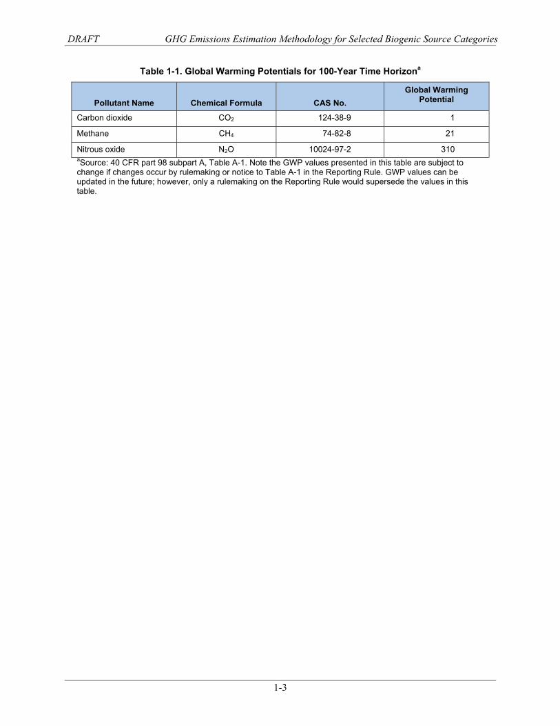
Table 1-1. Global Warming Potentials for 100-Year Time Horizona
Pollutant Name Chemical Formula CAS No. Global Warming
Potential
Carbon dioxide CO2 124-38-9 1
Methane CH4 74-82-8 21
Nitrous oxide N2O 10024-97-2 310 aSource: 40 CFR part 98 subpart A, Table A-1. Note the GWP values presented in this table are subject to change if changes occur by rulemaking or notice to Table A-1 in the Reporting Rule. GWP values can be updated in the future; however, only a rulemaking on the Reporting Rule would supersede the values in this table.
DRAFT GHG Emissions Estimation Methodology for Selected Biogenic Source Categories
1-4
[This page intentionally left blank]
DRAFT GHG Emissions Estimation Methodology for Selected Biogenic Source Categories
2-1
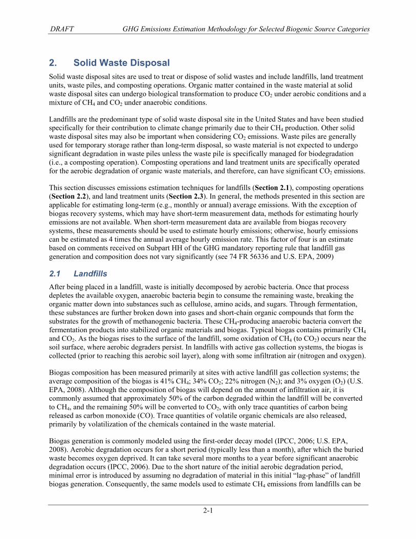
2. Solid Waste Disposal Solid waste disposal sites are used to treat or dispose of solid wastes and include landfills, land treatment units, waste piles, and composting operations. Organic matter contained in the waste material at solid waste disposal sites can undergo biological transformation to produce CO2 under aerobic conditions and a mixture of CH4 and CO2 under anaerobic conditions.
Landfills are the predominant type of solid waste disposal site in the United States and have been studied specifically for their contribution to climate change primarily due to their CH4 production. Other solid waste disposal sites may also be important when considering CO2 emissions. Waste piles are generally used for temporary storage rather than long-term disposal, so waste material is not expected to undergo significant degradation in waste piles unless the waste pile is specifically managed for biodegradation (i.e., a composting operation). Composting operations and land treatment units are specifically operated for the aerobic degradation of organic waste materials, and therefore, can have significant CO2 emissions.
This section discusses emissions estimation techniques for landfills (Section 2.1), composting operations (Section 2.2), and land treatment units (Section 2.3). In general, the methods presented in this section are applicable for estimating long-term (e.g., monthly or annual) average emissions. With the exception of biogas recovery systems, which may have short-term measurement data, methods for estimating hourly emissions are not available. When short-term measurement data are available from biogas recovery systems, these measurements should be used to estimate hourly emissions; otherwise, hourly emissions can be estimated as 4 times the annual average hourly emission rate. This factor of four is an estimate based on comments received on Subpart HH of the GHG mandatory reporting rule that landfill gas generation and composition does not vary significantly (see 74 FR 56336 and U.S. EPA, 2009)
2.1 Landfills After being placed in a landfill, waste is initially decomposed by aerobic bacteria. Once that process depletes the available oxygen, anaerobic bacteria begin to consume the remaining waste, breaking the organic matter down into substances such as cellulose, amino acids, and sugars. Through fermentation, these substances are further broken down into gases and short-chain organic compounds that form the substrates for the growth of methanogenic bacteria. These CH B4-producing anaerobic bacteria convert the fermentation products into stabilized organic materials and biogas. Typical biogas contains primarily CH4 and CO2. As the biogas rises to the surface of the landfill, some oxidation of CH4 (to CO2) occurs near the soil surface, where aerobic degraders persist. In landfills with active gas collection systems, the biogas is collected (prior to reaching this aerobic soil layer), along with some infiltration air (nitrogen and oxygen).
Biogas composition has been measured primarily at sites with active landfill gas collection systems; the average composition of the biogas is 41% CH4; 34% CO2; 22% nitrogen (N2); and 3% oxygen (O2) (U.S. EPA, 2008). Although the composition of biogas will depend on the amount of infiltration air, it is commonly assumed that approximately 50% of the carbon degraded within the landfill will be converted to CH4, and the remaining 50% will be converted to CO2, with only trace quantities of carbon being released as carbon monoxide (CO). Trace quantities of volatile organic chemicals are also released, primarily by volatilization of the chemicals contained in the waste material.
Biogas generation is commonly modeled using the first-order decay model (IPCC, 2006; U.S. EPA, 2008). Aerobic degradation occurs for a short period (typically less than a month), after which the buried waste becomes oxygen deprived. It can take several more months to a year before significant anaerobic degradation occurs (IPCC, 2006). Due to the short nature of the initial aerobic degradation period, minimal error is introduced by assuming no degradation of material in this initial “lag-phase” of landfill biogas generation. Consequently, the same models used to estimate CH4 emissions from landfills can be
DRAFT GHG Emissions Estimation Methodology for Selected Biogenic Source Categories
2-2
used to estimate CO2 emissions from landfills. The Landfill Gas Emission Model (LandGEM, v3.02; U.S. EPA, 2005) calculates CO2 emissions from landfills assuming that the volume of CO2 released equals the volume of CH4 as a default (CH4 content = 50% by volume). LandGEM does not specifically account for additional soil oxidation of CH4. In developing the U.S. inventory of CH4 emissions from landfills, it was assumed that 10% of the CH4 in uncaptured landfill gas is converted to CO2 (U.S. EPA, 2010a).
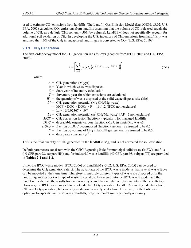
2.1.1 CH4 Generation The first-order decay model for CH4 generation is as follows (adapted from IPCC, 2006 and U.S. EPA, 2008):
( ){ }⎥⎦
⎤⎢⎣
⎡−= ∑
−
=
−−−−−1
)()1('T
Sx
xTkxTkxx eeLWA (2-1)
where
A = CH4 generation (Mg/yr) x = Year in which waste was disposed S = Start year of inventory calculation T = Inventory year for which emissions are calculated Wx = the quantity of waste disposed at the solid waste disposal site (Mg) L’ = CH4 generation potential (Mg CH4/Mg waste) = MCF × DOC × DOCF × F × 16 / 12 [IPCC nomenclature] = L0 × 16/0.02367 × 10-6 L0 = CH4 generation potential (m3 CH4/Mg waste) [AP-42 nomenclature] MCF = CH4 correction factor (fraction), typically 1 for managed landfills DOC = degradable organic carbon [fraction (Mg C in waste/Mg waste)] DOCF = fraction of DOC decomposed (fraction), generally assumed to be 0.5 F = fraction by volume of CH4 in landfill gas, generally assumed to be 0.5 k = decay rate constant (yr-1).
This is the total quantity of CH4 generated in the landfill in Mg, and is not corrected for soil oxidation.
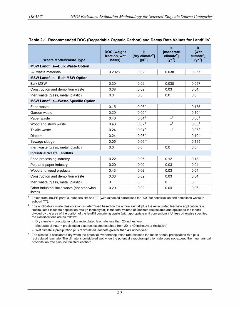
Default parameters consistent with the GHG Reporting Rule for municipal solid waste (MSW) landfills (40 CFR part 98, subpart HH) and for industrial waste landfills (40 CFR part 98, subpart TT) are provided in Tables 2-1 and 2-2.
Either the IPCC waste model (IPCC, 2006) or LandGEM (v3.02; U.S. EPA, 2005) can be used to determine the CH4 generation rate, A. The advantage of the IPCC waste model is that several waste types can be modeled at the same time. Therefore, if multiple different types of waste are disposed of in the landfill, quantities for each type of waste material can be entered into the IPCC waste model and the model will calculate the results for each waste type and the cumulative total quantity in the Results tab. However, the IPCC waste model does not calculate CO2 generation. LandGEM directly calculates both CH4 and CO2 generation, but can only model one waste type at a time. However, for the bulk waste option or for specific industrial waste landfills, only one model run is generally necessary.
DRAFT GHG Emissions Estimation Methodology for Selected Biogenic Source Categories
2-3
Table 2-1. Recommended DOC (Degradable Organic Carbon) and Decay Rate Values for Landfillsa
Waste Model/Waste Type
DOC (weight fraction, wet
basis)
k [dry climateb]
(yr-1)
k [moderate climateb]
(yr-1)
k [wet
climateb] (yr-1)
MSW Landfills—Bulk Waste Option All waste materials 0.2028 0.02 0.038 0.057 MSW Landfills—Bulk MSW Option Bulk MSW 0.30 0.02 0.038 0.057 Construction and demolition waste 0.08 0.02 0.03 0.04 Inert waste (glass, metal, plastic) 0.0 0.0 0.0 0.0 MSW Landfills—Waste-Specific Option Food waste 0.15 0.06 c –c 0.185 c Garden waste 0.20 0.05 c –c 0.10 c Paper waste 0.40 0.04 c –c 0.06 c Wood and straw waste 0.43 0.02 c –c 0.03 c Textile waste 0.24 0.04 c –c 0.06 c Diapers 0.24 0.05 c –c 0.10 c Sewage sludge 0.05 0.06 c –c 0.185 c Inert waste (glass, metal, plastic) 0.0 0.0 0.0 0.0 Industrial Waste Landfills Food processing industry 0.22 0.06 0.12 0.18 Pulp and paper industry 0.20 0.02 0.03 0.04 Wood and wood products 0.43 0.02 0.03 0.04 Construction and demolition waste 0.08 0.02 0.03 0.04 Inert waste (glass, metal, plastic) 0 0 0 0 Other industrial solid waste (not otherwise listed)
0.20 0.02 0.04 0.06
a Taken from 40CFR part 98, subparts HH and TT (with expected corrections for DOC for construction and demolition waste in subpart TT).
b The applicable climate classification is determined based on the annual rainfall plus the recirculated leachate application rate. Recirculated leachate application rate (in inches/year) is the total volume of leachate recirculated and applied to the landfill divided by the area of the portion of the landfill containing waste (with appropriate unit conversions). Unless otherwise specified, the classifications are as follows: – Dry climate = precipitation plus recirculated leachate less than 20 inches/year – Moderate climate = precipitation plus recirculated leachate from 20 to 40 inches/year (inclusive) – Wet climate = precipitation plus recirculated leachate greater than 40 inches/year.
c The climate is considered dry when the potential evapotranspiration rate exceeds the mean annual precipitation rate plus recirculated leachate. The climate is considered wet when the potential evapotranspiration rate does not exceed the mean annual precipitation rate plus recirculated leachate.
DRAFT GHG Emissions Estimation Methodology for Selected Biogenic Source Categories
2-4
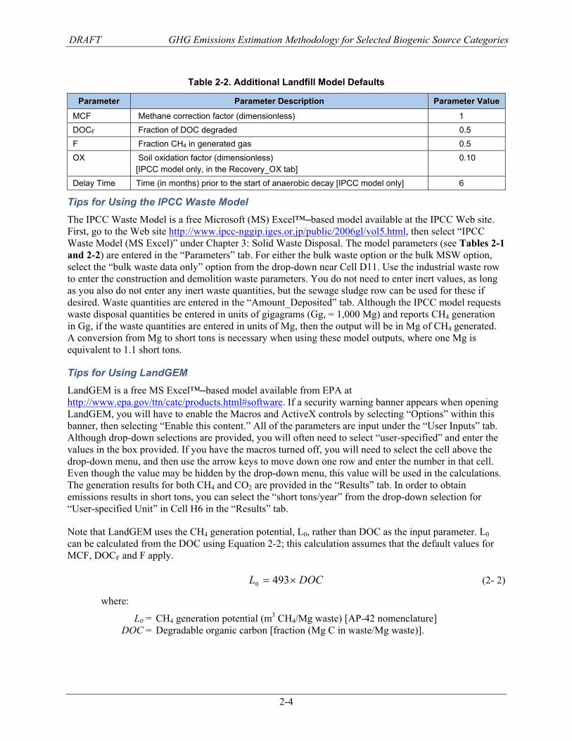
Table 2-2. Additional Landfill Model Defaults
Parameter Parameter Description Parameter Value
MCF Methane correction factor (dimensionless) 1 DOCF Fraction of DOC degraded 0.5 F Fraction CH4 in generated gas 0.5 OX Soil oxidation factor (dimensionless)
[IPCC model only, in the Recovery_OX tab] 0.10
Delay Time Time (in months) prior to the start of anaerobic decay [IPCC model only] 6
Tips for Using the IPCC Waste Model The IPCC Waste Model is a free Microsoft (MS) Excel™–based model available at the IPCC Web site. First, go to the Web site http://www.ipcc-nggip.iges.or.jp/public/2006gl/vol5.html, then select “IPCC Waste Model (MS Excel)” under Chapter 3: Solid Waste Disposal. The model parameters (see Tables 2-1 and 2-2) are entered in the “Parameters” tab. For either the bulk waste option or the bulk MSW option, select the “bulk waste data only” option from the drop-down near Cell D11. Use the industrial waste row to enter the construction and demolition waste parameters. You do not need to enter inert values, as long as you also do not enter any inert waste quantities, but the sewage sludge row can be used for these if desired. Waste quantities are entered in the “Amount_Deposited” tab. Although the IPCC model requests waste disposal quantities be entered in units of gigagrams (Gg, = 1,000 Mg) and reports CH4 generation in Gg, if the waste quantities are entered in units of Mg, then the output will be in Mg of CH4 generated. A conversion from Mg to short tons is necessary when using these model outputs, where one Mg is equivalent to 1.1 short tons.
Tips for Using LandGEM LandGEM is a free MS Excel™–based model available from EPA at http://www.epa.gov/ttn/catc/products.html#software. If a security warning banner appears when opening LandGEM, you will have to enable the Macros and ActiveX controls by selecting “Options” within this banner, then selecting “Enable this content.” All of the parameters are input under the “User Inputs” tab. Although drop-down selections are provided, you will often need to select “user-specified” and enter the values in the box provided. If you have the macros turned off, you will need to select the cell above the drop-down menu, and then use the arrow keys to move down one row and enter the number in that cell. Even though the value may be hidden by the drop-down menu, this value will be used in the calculations. The generation results for both CH4 and CO2 are provided in the “Results” tab. In order to obtain emissions results in short tons, you can select the “short tons/year” from the drop-down selection for “User-specified Unit” in Cell H6 in the “Results” tab.
Note that LandGEM uses the CH4 generation potential, L0, rather than DOC as the input parameter. L0 can be calculated from the DOC using Equation 2-2; this calculation assumes that the default values for MCF, DOCF and F apply.
DOCL ×= 4930 (2- 2)
where:
L0 = CH4 generation potential (m3 CH4/Mg waste) [AP-42 nomenclature] DOC = Degradable organic carbon [fraction (Mg C in waste/Mg waste)].

DRAFT GHG Emissions Estimation Methodology for Selected Biogenic Source Categories
2-5
Note also that LandGEM calculates only CH4 and CO2 generation without accounting for soil oxidation. It is generally assumed that 10% of the CH4 generated is oxidized to CO2 near the surface of the landfill (U.S. EPA, 2010a), so that CH4 emissions (with no gas collection) are 90% of CH4 generation.
2.1.2 CO2 Emissions for Landfills without Gas Collection Systems For landfills without gas collection systems, CO2 emissions can be calculated from the CH4 generation as follows:
16441
×⎟⎠⎞
⎜⎝⎛ +−
×= OXF
FAB (2- 3)
where:
B = CO2 emissions (Mg/yr) A = CH4 generation from Equation 2-1 (Mg CH4/yr) F = Fraction by volume of CH4 in landfill gas, generally assumed to be 0.5
Sample Calculation for CH4 Generation at Landfills Problem: A food processing plant disposes of 10,000 Mg of waste a year in an on-site landfill. The landfill is in a moderate climate, has been accepting waste since 1983, and has no gas collection system. What are the CH4 emissions from the landfill in 2010? Solution: The following inputs are given:
S = 1983 T = 2010 Wx = 10,000 Mg for each year from 1983 through 2010
From Table 2-1, we have DOC = 0.22 (Industrial waste landfill, food processing industry) k = 0.12 yr-1 (Industrial waste landfill, food processing industry, moderate climate)
Use Equation 2-2 to convert DOC to L0 for use in LandGEM: L0 = 493 × 0.22 = 108.5 m3 CH4/Mg waste
Select the “User Inputs” tab. Enter “1983” in Cell D5; enter “2010” or larger number in Cell D6; enter 0.12 for k and 108.5 for L0. The selection of the concentration of non-methane organic compounds (NMOC concentration) will not affect the CH4 or CO2 calculations; use the default value for CH4 content, F, of 50%. Make sure the drop down box at Cell K4 indicates waste quantities in Mg/yr, then enter 10,000 in Cells K8 through K35 (the latter should indicate year 2010). Use the default reporting profile under the section “Selected Gases/Pollutants” (this will provide output for both CH4 and CO2). Select the “Results” tab. CH4 generation, A, for 2010 is reported in Cell I-36 (using the default pollutant reporting profile).
A = 700 Mg CH4 in 2010 It is assumed that 10% of the CH4 generated will oxidize near the landfill surface, so the CH4 emissions would be 700 × (1 – 0.1) = 630 Mg CH4/yr for 2010. Converting the CH4 emissions (GWP = 21) to CO2e:
CH4 emissions are 630 × 21 = 13,230 Mg CO2e/yr Converting to short tons:
CH4 emissions are 13,230 Mg CO2e/yr × 1.1 t/Mg = 14,553 tpy CO2e = 14,600 tpy CO2e rounded to three significant figures.
DRAFT GHG Emissions Estimation Methodology for Selected Biogenic Source Categories
2-6
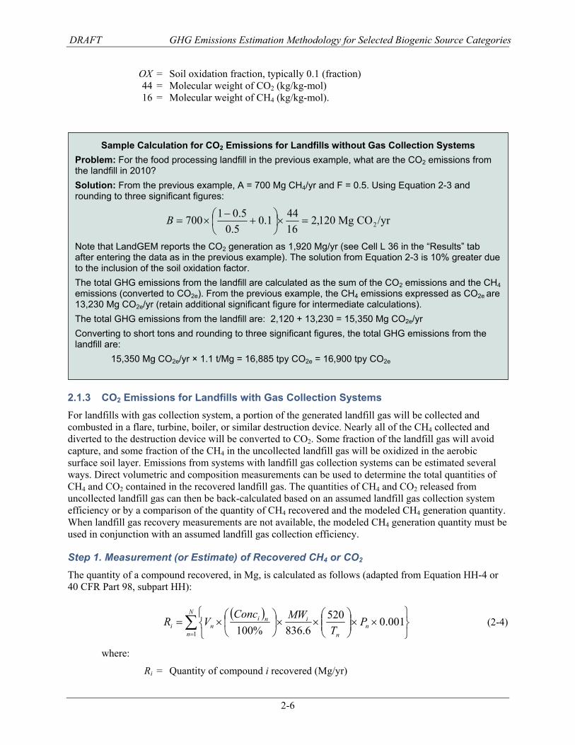
OX = Soil oxidation fraction, typically 0.1 (fraction) 44 = Molecular weight of CO2 (kg/kg-mol) 16 = Molecular weight of CH4 (kg/kg-mol).
2.1.3 CO2 Emissions for Landfills with Gas Collection Systems For landfills with gas collection system, a portion of the generated landfill gas will be collected and combusted in a flare, turbine, boiler, or similar destruction device. Nearly all of the CH4 collected and diverted to the destruction device will be converted to CO2. Some fraction of the landfill gas will avoid capture, and some fraction of the CH4 in the uncollected landfill gas will be oxidized in the aerobic surface soil layer. Emissions from systems with landfill gas collection systems can be estimated several ways. Direct volumetric and composition measurements can be used to determine the total quantities of CH4 and CO2 contained in the recovered landfill gas. The quantities of CH4 and CO2 released from uncollected landfill gas can then be back-calculated based on an assumed landfill gas collection system efficiency or by a comparison of the quantity of CH4 recovered and the modeled CH4 generation quantity. When landfill gas recovery measurements are not available, the modeled CH4 generation quantity must be used in conjunction with an assumed landfill gas collection efficiency.
Step 1. Measurement (or Estimate) of Recovered CH4 or CO2
The quantity of a compound recovered, in Mg, is calculated as follows (adapted from Equation HH-4 or 40 CFR Part 98, subpart HH):
( )
∑= ⎭
⎬⎫
⎩⎨⎧
××⎟⎟⎠
⎞⎜⎜⎝
⎛××⎟
⎠
⎞⎜⎝
⎛×=
N
nn
n
inini P
TMWConc
VR1
001.05206.836%100
(2-4)
where:
Ri = Quantity of compound i recovered (Mg/yr)
Sample Calculation for CO2 Emissions for Landfills without Gas Collection Systems Problem: For the food processing landfill in the previous example, what are the CO2 emissions from the landfill in 2010? Solution: From the previous example, A = 700 Mg CH4/yr and F = 0.5. Using Equation 2-3 and rounding to three significant figures:
/yrCOMg120,216441.0
5.05.01700 2=×⎟
⎠⎞
⎜⎝⎛ +−
×=B
Note that LandGEM reports the CO2 generation as 1,920 Mg/yr (see Cell L 36 in the “Results” tab after entering the data as in the previous example). The solution from Equation 2-3 is 10% greater due to the inclusion of the soil oxidation factor. The total GHG emissions from the landfill are calculated as the sum of the CO2 emissions and the CH4 emissions (converted to CO2e). From the previous example, the CH4 emissions expressed as CO2e are 13,230 Mg CO2e/yr (retain additional significant figure for intermediate calculations). The total GHG emissions from the landfill are: 2,120 + 13,230 = 15,350 Mg CO2e/yr Converting to short tons and rounding to three significant figures, the total GHG emissions from the landfill are:
15,350 Mg CO2e/yr × 1.1 t/Mg = 16,885 tpy CO2e = 16,900 tpy CO2e
DRAFT GHG Emissions Estimation Methodology for Selected Biogenic Source Categories
2-7
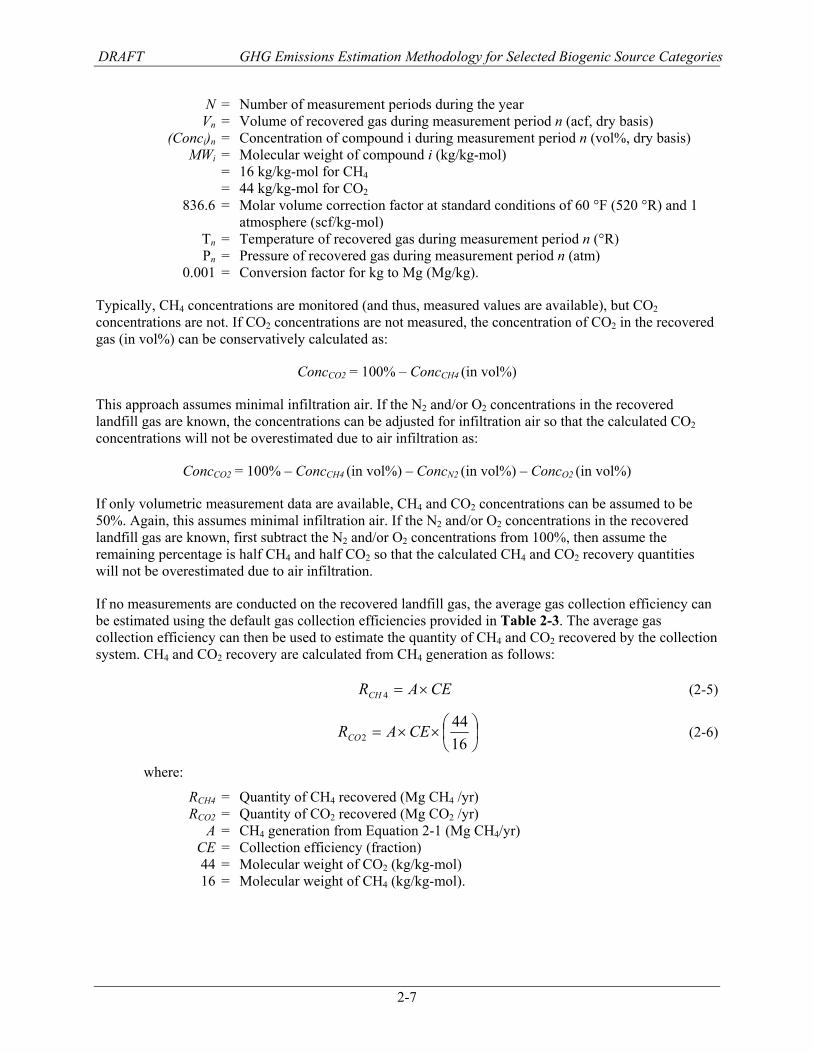
N = Number of measurement periods during the year Vn = Volume of recovered gas during measurement period n (acf, dry basis) (Conci)n = Concentration of compound i during measurement period n (vol%, dry basis) MWi = Molecular weight of compound i (kg/kg-mol) = 16 kg/kg-mol for CH4 = 44 kg/kg-mol for CO2 836.6 = Molar volume correction factor at standard conditions of 60 °F (520 °R) and 1
atmosphere (scf/kg-mol) Tn = Temperature of recovered gas during measurement period n (°R) Pn = Pressure of recovered gas during measurement period n (atm) 0.001 = Conversion factor for kg to Mg (Mg/kg).
Typically, CH4 concentrations are monitored (and thus, measured values are available), but CO2 concentrations are not. If CO2 concentrations are not measured, the concentration of CO2 in the recovered gas (in vol%) can be conservatively calculated as:
ConcCO2 = 100% – ConcCH4 (in vol%)
This approach assumes minimal infiltration air. If the N2 and/or O2 concentrations in the recovered landfill gas are known, the concentrations can be adjusted for infiltration air so that the calculated CO2 concentrations will not be overestimated due to air infiltration as:
ConcCO2 = 100% – ConcCH4 (in vol%) – ConcN2 (in vol%) – ConcO2 (in vol%)
If only volumetric measurement data are available, CH4 and CO2 concentrations can be assumed to be 50%. Again, this assumes minimal infiltration air. If the N2 and/or O2 concentrations in the recovered landfill gas are known, first subtract the N2 and/or O2 concentrations from 100%, then assume the remaining percentage is half CH4 and half CO2 so that the calculated CH4 and CO2 recovery quantities will not be overestimated due to air infiltration.
If no measurements are conducted on the recovered landfill gas, the average gas collection efficiency can be estimated using the default gas collection efficiencies provided in Table 2-3. The average gas collection efficiency can then be used to estimate the quantity of CH4 and CO2 recovered by the collection system. CH4 and CO2 recovery are calculated from CH4 generation as follows:
CEARCH ×=4 (2-5)
⎟⎠⎞
⎜⎝⎛××=
1644
2 CEARCO (2-6)
where:
RCH4 = Quantity of CH4 recovered (Mg CH4 /yr) RCO2 = Quantity of CO2 recovered (Mg CO2 /yr) A = CH4 generation from Equation 2-1 (Mg CH4/yr) CE = Collection efficiency (fraction) 44 = Molecular weight of CO2 (kg/kg-mol) 16 = Molecular weight of CH4 (kg/kg-mol).
DRAFT GHG Emissions Estimation Methodology for Selected Biogenic Source Categories
2-8
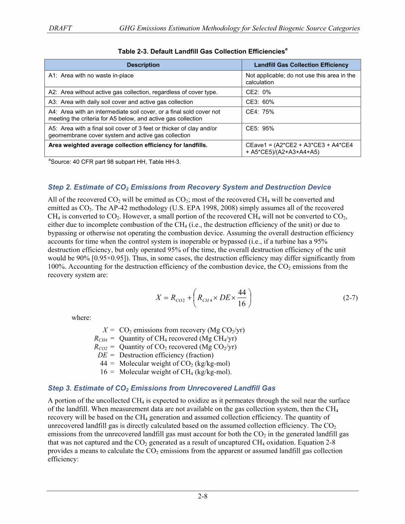
Table 2-3. Default Landfill Gas Collection Efficienciesa
Description Landfill Gas Collection Efficiency
A1: Area with no waste in-place Not applicable; do not use this area in the calculation
A2: Area without active gas collection, regardless of cover type. CE2: 0% A3: Area with daily soil cover and active gas collection CE3: 60% A4: Area with an intermediate soil cover, or a final sold cover not meeting the criteria for A5 below, and active gas collection
CE4: 75%
A5: Area with a final soil cover of 3 feet or thicker of clay and/or geomembrane cover system and active gas collection
CE5: 95%
Area weighted average collection efficiency for landfills. CEave1 = (A2*CE2 + A3*CE3 + A4*CE4 + A5*CE5)/(A2+A3+A4+A5)
aSource: 40 CFR part 98 subpart HH, Table HH-3.
Step 2. Estimate of CO2 Emissions from Recovery System and Destruction Device All of the recovered CO2 will be emitted as CO2; most of the recovered CH4 will be converted and emitted as CO2. The AP-42 methodology (U.S. EPA 1998, 2008) simply assumes all of the recovered CH4 is converted to CO2. However, a small portion of the recovered CH4 will not be converted to CO2, either due to incomplete combustion of the CH4 (i.e., the destruction efficiency of the unit) or due to bypassing or otherwise not operating the combustion device. Assuming the overall destruction efficiency accounts for time when the control system is inoperable or bypassed (i.e., if a turbine has a 95% destruction efficiency, but only operated 95% of the time, the overall destruction efficiency of the unit would be 90% [0.95×0.95]). Thus, in some cases, the destruction efficiency may differ significantly from 100%. Accounting for the destruction efficiency of the combustion device, the CO2 emissions from the recovery system are:
⎟⎠⎞
⎜⎝⎛ ××+=
1644
42 DERRX CHCO (2-7)
where:
X = CO2 emissions from recovery (Mg CO2/yr) RCH4 = Quantity of CH4 recovered (Mg CH4/yr) RCO2 = Quantity of CO2 recovered (Mg CO2/yr) DE = Destruction efficiency (fraction) 44 = Molecular weight of CO2 (kg/kg-mol) 16 = Molecular weight of CH4 (kg/kg-mol).
Step 3. Estimate of CO2 Emissions from Unrecovered Landfill Gas A portion of the uncollected CH4 is expected to oxidize as it permeates through the soil near the surface of the landfill. When measurement data are not available on the gas collection system, then the CH4 recovery will be based on the CH4 generation and assumed collection efficiency. The quantity of unrecovered landfill gas is directly calculated based on the assumed collection efficiency. The CO2 emissions from the unrecovered landfill gas must account for both the CO2 in the generated landfill gas that was not captured and the CO2 generated as a result of uncaptured CH4 oxidation. Equation 2-8 provides a means to calculate the CO2 emissions from the apparent or assumed landfill gas collection efficiency:
DRAFT GHG Emissions Estimation Methodology for Selected Biogenic Source Categories
2-9
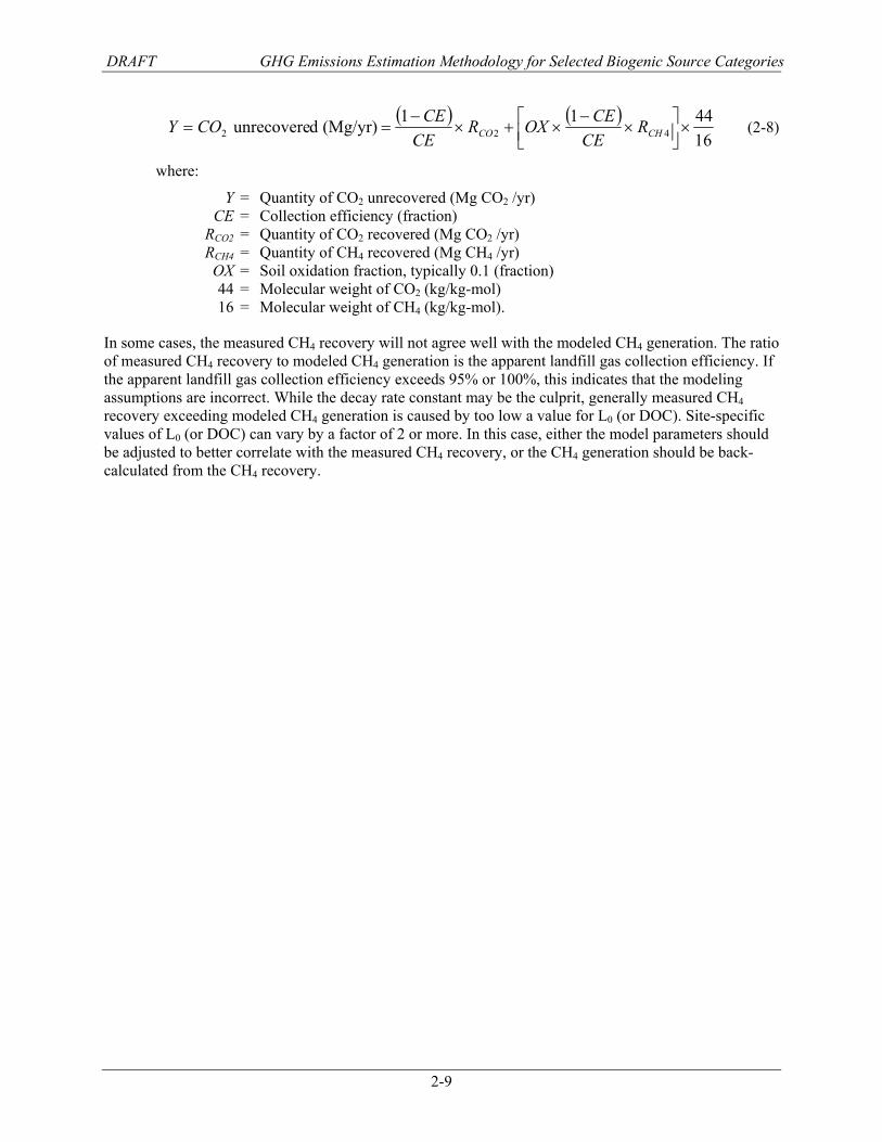
( ) ( )
164411(Mg/yr)dunrecovere 422 ×⎥⎦
⎤⎢⎣⎡ ×
−×+×
−== CHCO R
CECEOXR
CECECOY (2-8)
where:
Y = Quantity of CO2 unrecovered (Mg CO2 /yr) CE = Collection efficiency (fraction) RCO2 = Quantity of CO2 recovered (Mg CO2 /yr) RCH4 = Quantity of CH4 recovered (Mg CH4 /yr) OX = Soil oxidation fraction, typically 0.1 (fraction) 44 = Molecular weight of CO2 (kg/kg-mol) 16 = Molecular weight of CH4 (kg/kg-mol).
In some cases, the measured CH4 recovery will not agree well with the modeled CH4 generation. The ratio of measured CH4 recovery to modeled CH4 generation is the apparent landfill gas collection efficiency. If the apparent landfill gas collection efficiency exceeds 95% or 100%, this indicates that the modeling assumptions are incorrect. While the decay rate constant may be the culprit, generally measured CH4 recovery exceeding modeled CH4 generation is caused by too low a value for L0 (or DOC). Site-specific values of L0 (or DOC) can vary by a factor of 2 or more. In this case, either the model parameters should be adjusted to better correlate with the measured CH4 recovery, or the CH4 generation should be back-calculated from the CH4 recovery.
DRAFT GHG Emissions Estimation Methodology for Selected Biogenic Source Categories
2-10
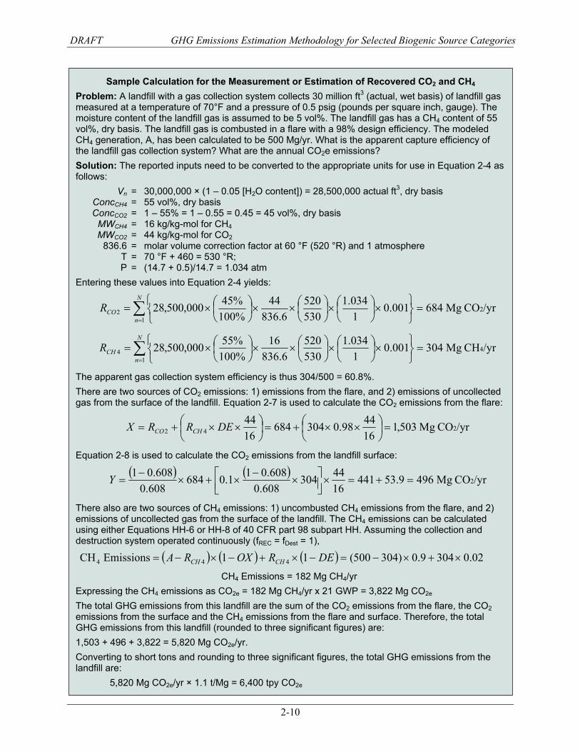
Sample Calculation for the Measurement or Estimation of Recovered CO2 and CH4 Problem: A landfill with a gas collection system collects 30 million ft3 (actual, wet basis) of landfill gas measured at a temperature of 70°F and a pressure of 0.5 psig (pounds per square inch, gauge). The moisture content of the landfill gas is assumed to be 5 vol%. The landfill gas has a CH4 content of 55 vol%, dry basis. The landfill gas is combusted in a flare with a 98% design efficiency. The modeled CH4 generation, A, has been calculated to be 500 Mg/yr. What is the apparent capture efficiency of the landfill gas collection system? What are the annual CO2e emissions? Solution: The reported inputs need to be converted to the appropriate units for use in Equation 2-4 as follows: Vn = 30,000,000 × (1 – 0.05 [H2O content]) = 28,500,000 actual ft3, dry basis ConcCH4 = 55 vol%, dry basis ConcCO2 = 1 – 55% = 1 – 0.55 = 0.45 = 45 vol%, dry basis MWCH4 = 16 kg/kg-mol for CH4 MWCO2 = 44 kg/kg-mol for CO2 836.6 = molar volume correction factor at 60 °F (520 °R) and 1 atmosphere T = 70 °F + 460 = 530 °R; P = (14.7 + 0.5)/14.7 = 1.034 atm Entering these values into Equation 2-4 yields:
/yrCO Mg684001.01034.1
530520
6.83644
%100%45000,500,28 2
12 =
⎭⎬⎫
⎩⎨⎧
×⎟⎠⎞
⎜⎝⎛×⎟
⎠⎞
⎜⎝⎛××⎟
⎠⎞
⎜⎝⎛×= ∑
=
N
nCOR
/yrCH Mg304001.01034.1
530520
6.83616
%100%55000,500,28 4
14 =
⎭⎬⎫
⎩⎨⎧
×⎟⎠⎞
⎜⎝⎛×⎟
⎠⎞
⎜⎝⎛××⎟
⎠⎞
⎜⎝⎛×= ∑
=
N
nCHR
The apparent gas collection system efficiency is thus 304/500 = 60.8%. There are two sources of CO2 emissions: 1) emissions from the flare, and 2) emissions of uncollected gas from the surface of the landfill. Equation 2-7 is used to calculate the CO2 emissions from the flare:
/yrCO Mg503,1164498.0304684
1644
242 =⎟⎠⎞
⎜⎝⎛ ××+=⎟
⎠⎞
⎜⎝⎛ ××+= DERRX CHCO
Equation 2-8 is used to calculate the CO2 emissions from the landfill surface:
( ) ( ) /yrCO Mg4969.53441
1644304
608.0608.011.0684
608.0608.01
2=+=×⎥⎦⎤
⎢⎣⎡ ×
−×+×
−=Y
There also are two sources of CH4 emissions: 1) uncombusted CH4 emissions from the flare, and 2) emissions of uncollected gas from the surface of the landfill. The CH4 emissions can be calculated using either Equations HH-6 or HH-8 of 40 CFR part 98 subpart HH. Assuming the collection and destruction system operated continuously (fREC = fDest = 1),
( ) ( ) ( ) 02.03049.0)304500(11Emissions CH 444 ×+×−=−×+−×−= DEROXRA CHCH
CH4 Emissions = 182 Mg CH4/yr Expressing the CH4 emissions as CO2e = 182 Mg CH4/yr x 21 GWP = 3,822 Mg CO2e The total GHG emissions from this landfill are the sum of the CO2 emissions from the flare, the CO2 emissions from the surface and the CH4 emissions from the flare and surface. Therefore, the total GHG emissions from this landfill (rounded to three significant figures) are: 1,503 + 496 + 3,822 = 5,820 Mg CO2e/yr. Converting to short tons and rounding to three significant figures, the total GHG emissions from the landfill are:
5,820 Mg CO2e/yr × 1.1 t/Mg = 6,400 tpy CO2e
DRAFT GHG Emissions Estimation Methodology for Selected Biogenic Source Categories
2-11
2.2 Composting Operations
Composting is a specific waste management process by which organic waste is aerobically converted to a stabilized solid product called compost, which can then be used a fertilizer or soil amendment. There are three common methods of composting:
Windrow composting—waste material is placed in rows of long piles called "windrows" and aerated by turning the pile periodically by either manual or mechanical means.
Aerated static pile composting—waste materials are placed in a single waste pile with layers of loosely piled bulking agents (e.g., wood chips, shredded newspaper) so that air can pass from the bottom to the top of the pile. The piles also can be placed over a network of pipes that deliver air into or draw air out of the pile.
In-vessel composting—organic materials are fed into a drum, silo, or similar equipment where the environmental conditions (including temperature, moisture, and aeration) are closely controlled. The apparatus usually has a mechanism to turn or agitate the material for proper aeration.
Composting facilities manage waste on a short-term basis (compared to landfills), so there is no need to track the quantity of waste managed over historic years. Additionally, while a small fraction of carbon in the waste may be converted to CH4 in anaerobic sections within composting piles when there is excessive moisture or inadequate aeration (or mixing), most of the generated CH4 is oxidized in the aerobic sections of the compost. As such, most of the carbon degraded within the compost pile will be converted to CO2. Generally, there will be a reduction in both the mass and carbon content of material in the compost pile.
One approach to determining CO2 emissions from composting is to perform a careful carbon balance, considering carbon content and initial mass of raw waste materials and bulking materials added to the compost pile and a total mass and carbon content of the final compost. Typically, these data are not measured or available at most composting facilities. Volatile solids content can be used as a proxy for carbon content, but careful mass and volatile solids measurements would be required for all waste material, bulking agents, and final compost. These measurements are needed on a dry basis, so that changes in moisture content would not affect the results. In a study by Das et al. (1998), composting achieved approximately a 15% dry solids mass reduction and a 10% reduction in volatile solids content (of the dry solids) from the initial solids content. Therefore, composting achieved a 23.5% reduction in the initial mass of volatile solids (1 – 0.85×0.9). Based on data from Barlaz (1998), Das et al. (1998), and Zhang et al. (2007), the average ratio of carbon content to volatile solids content in waste materials (including bulking agents) is 0.53 (see U.S. EPA, 2010b for additional information on the derivation of this value). Using this carbon to volatile solids ratio and the mass reductions measured by Das et al. (1998), we estimate that 12% (23.5% × 0.53) of the total dry weight of solids added to a compost pile is carbon that is degraded during the composting process. Accounting for molecular weight of CO2, these data suggest that an appropriate CO2 emission factor for composting operations is 0.44 kg/kg dry solids (12% × 44/12). Therefore, when more direct mass balance measurements are not available, the annual CO2 emissions from composting facility can be estimated as:
( )∑=
××=N
nnncompostcompostCO TSMEFE
1,2 (2-9)
where:
ECO2 = CO2 emissions (Mg CO2/yr) EFcompost = CO2 emission factor for composted material (kg CO2/kg dry solids) = 0.44 kg CO2/kg dry solids n = Index for the waste material or bulking agent
DRAFT GHG Emissions Estimation Methodology for Selected Biogenic Source Categories
2-12
N = Total number of different waste materials added to the compost pile or process Mcompost,n = Annual mass of material n added or fed to the compost process (Mg/yr, wet
basis) TSn = Total solids content of material n when added or fed to the compost process (kg
dry solids/kg wet solids).
CH4 and N2O emissions from composting may be calculated using the total mass of waste composted and the emission factors provided in Table 2-4. Note that the emission factors for CH4 and N2O are provided on a wet basis, so the emissions are calculated directly from the mass of material composted on a wet basis as:
compostCHcompostCH MEFE ×= 4,4 (2-10)
compostONcompostON MEFE ×= 2,2 (2-11)
where:
ECH4 = CH4 emissions (Mg CH4/yr) EN2O = N2O emissions (Mg N2O/yr) EFcompost,CH4 = CH4 emission factor for composted material (kg CH4/kg wet waste) = 0.004 kg CH4/kg wet waste (see Table 2-4) EFcompost,N2O = N2O emission factor for composted material (kg N2O/kg wet waste) = 0.0003 kg N2O/kg wet waste (see Table 2-4) Mcompost = Annual mass of material added or fed to the compost process (Mg/yr, wet basis).
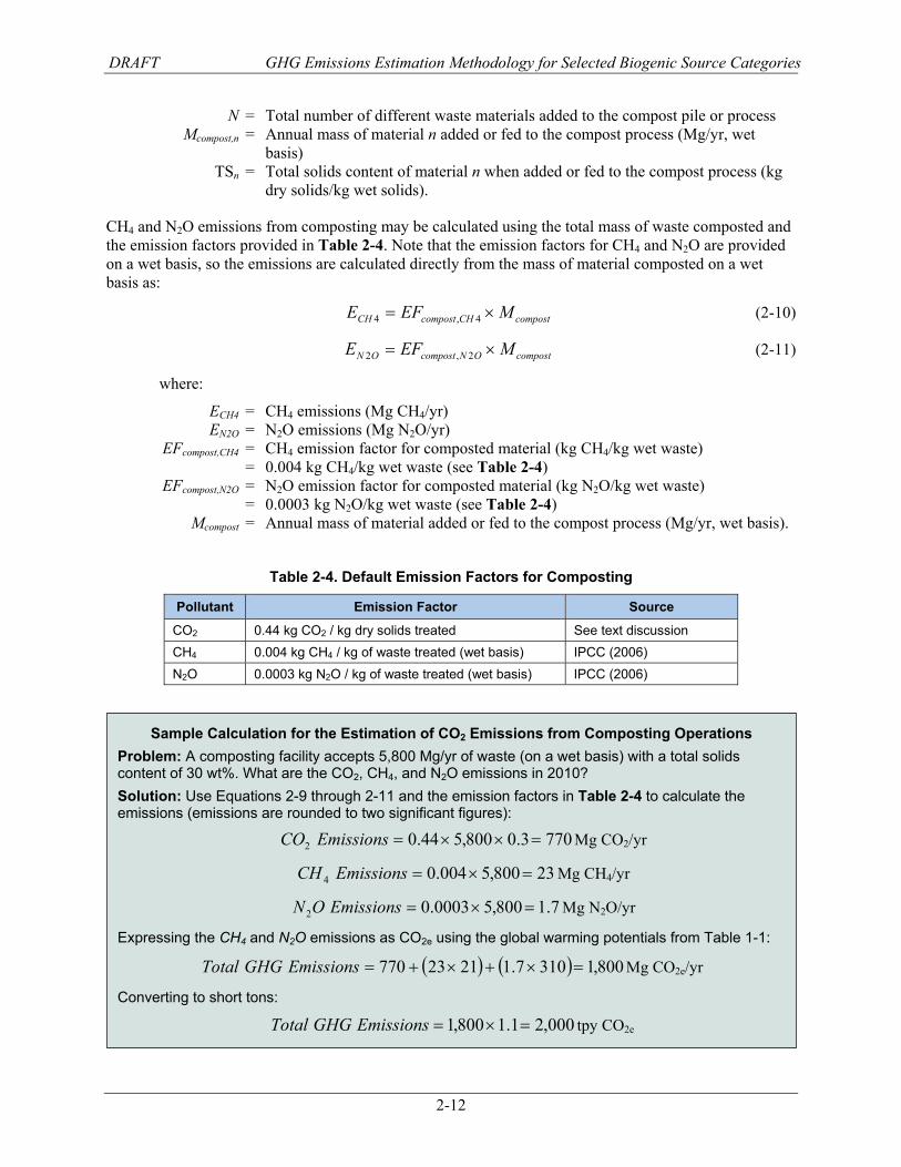
Table 2-4. Default Emission Factors for Composting
Pollutant Emission Factor Source
CO2 0.44 kg CO2 / kg dry solids treated See text discussion CH4 0.004 kg CH4 / kg of waste treated (wet basis) IPCC (2006) N2O 0.0003 kg N2O / kg of waste treated (wet basis) IPCC (2006)
Sample Calculation for the Estimation of CO2 Emissions from Composting Operations Problem: A composting facility accepts 5,800 Mg/yr of waste (on a wet basis) with a total solids content of 30 wt%. What are the CO2, CH4, and N2O emissions in 2010? Solution: Use Equations 2-9 through 2-11 and the emission factors in Table 2-4 to calculate the emissions (emissions are rounded to two significant figures):
7703.0800,544.02 =××=EmissionsCO Mg CO2/yr
23800,5004.04 =×=EmissionsCH Mg CH4/yr
7.1800,50003.02 =×=EmissionsON Mg N2O/yr
Expressing the CH4 and N2O emissions as CO2e using the global warming potentials from Table 1-1:
( ) ( ) 800,13107.12123770 =×+×+=EmissionsGHGTotal Mg CO2e/yr
Converting to short tons:
000,21.1800,1 =×=EmissionsGHGTotal tpy CO2e
DRAFT GHG Emissions Estimation Methodology for Selected Biogenic Source Categories
2-13
2.3 Land Treatment Units Land treatment units (also known as land application units) are large areas of land where waste is applied or incorporated with the soil near the surface of the land (tilling depth of 6 to 12 inches). The soil is commonly re-tilled at fixed intervals to help aerate and further mix the waste/soil layer. Unlike composting, a land treatment unit is used for the final disposal of the waste material. Land treatment units are often used for the disposal of biosolids and petroleum sludge. Carbon in the applied wastes is converted to CO2 and new biomass. Assuming a constant biomass population (dying and decaying biomass equaling new biomass growth), the CO2 generation rate from the land treatment unit will be directly proportional to the carbon application rate to the land treatment unit:
1244
2 ×××= wwwCO CCTSME (2-12)
where:
ECO2 = Annual CO2 emissions (Mg CO2/yr) Mw = Annual mass of waste applied to the land treatment unit (Mg/yr, wet basis); TSw = Total solids content of waste material applied to the land treatment unit (kg dry
solids/kg wet solids). CCw = Carbon content of waste material applied to the land treatment unit (kg C/kg dry
solids) 44 = Molecular weight of CO2 (kg/kg-mol) 12 = Molecular weight of carbon (kg/kg-mol).
Sample Calculation for the Estimation of CO2 Emissions from Land Treatment Units Problem: A facility applies 500,000 Mg/yr of waste to a land treatment unit. The applied waste has a moisture content of 20 wt% and a carbon content of 40 wt% (dry basis). What are the annual CO2 emissions from the land treatment unit? Solution: First, calculate the solids content as 1 – moisture content = 0.80 kg/kg waste, then apply Equation 2-11, as follows:
Mg/yr587,000
124440.080.0000,500)/(2 =×××=yrMgEmissionsCO
Converting to short tons:
tpy646,0001.1000,587)(2 =×=tpyEmissionsCO
DRAFT GHG Emissions Estimation Methodology for Selected Biogenic Source Categories
2-14
[This page intentionally left blank]
DRAFT GHG Emissions Estimation Methodology for Selected Biogenic Source Categories
3-1
3. Wastewater Treatment Wastewater treatment systems are designed to remove soluble organic matter, suspended solids, pathogenic organisms, and chemical contaminants in wastewaters before the water can be discharged into natural water systems. Wastewater treatment systems used to treat household wastewater and sewage are referred to as municipal wastewater treatment systems. Wastewater treatment systems used to treat wastewater generated at an industrial facility are referred to as industrial wastewater treatment systems. Both municipal and industrial wastewater treatment systems may include a variety of processes, ranging from primary treatment for solids removal to secondary biological treatment (e.g., activated sludge, lagoons) for organics reduction to tertiary treatment for nutrient removal, disinfection, and more discrete filtration. Biological treatment is an effective process for reducing, removing, or transforming organic constituents and nutrients typically found in wastewaters to an acceptable form or concentration prior to discharge or reuse. As such, biological treatment systems are widely used in the United States for both municipal and industrial wastewater treatment.
When considering CO2 emissions from wastewater treatment systems, there are two primary classes of biological treatment units: aerobic treatment units and anaerobic treatment units. Some treatment units, such as facultative lagoons, may be a mixture of the two, with aerobic zones near the surface of the lagoon and anaerobic zones in the lower depths of the lagoon. Regardless of the type of biological treatment employed, the biochemical reactions are similar, with organic carbon compounds being oxidized to form new cells, CO2 and/or CH4, and water. This section provides a basic introduction to some of the primary types of biological wastewater treatment systems (Section 3.1), a method of estimating CO2 and CH4 emissions from biological wastewater treatment systems (Section 3.2), and a method of estimating N2O emissions (Section 3.3).
3.1 Biological Treatment Processes
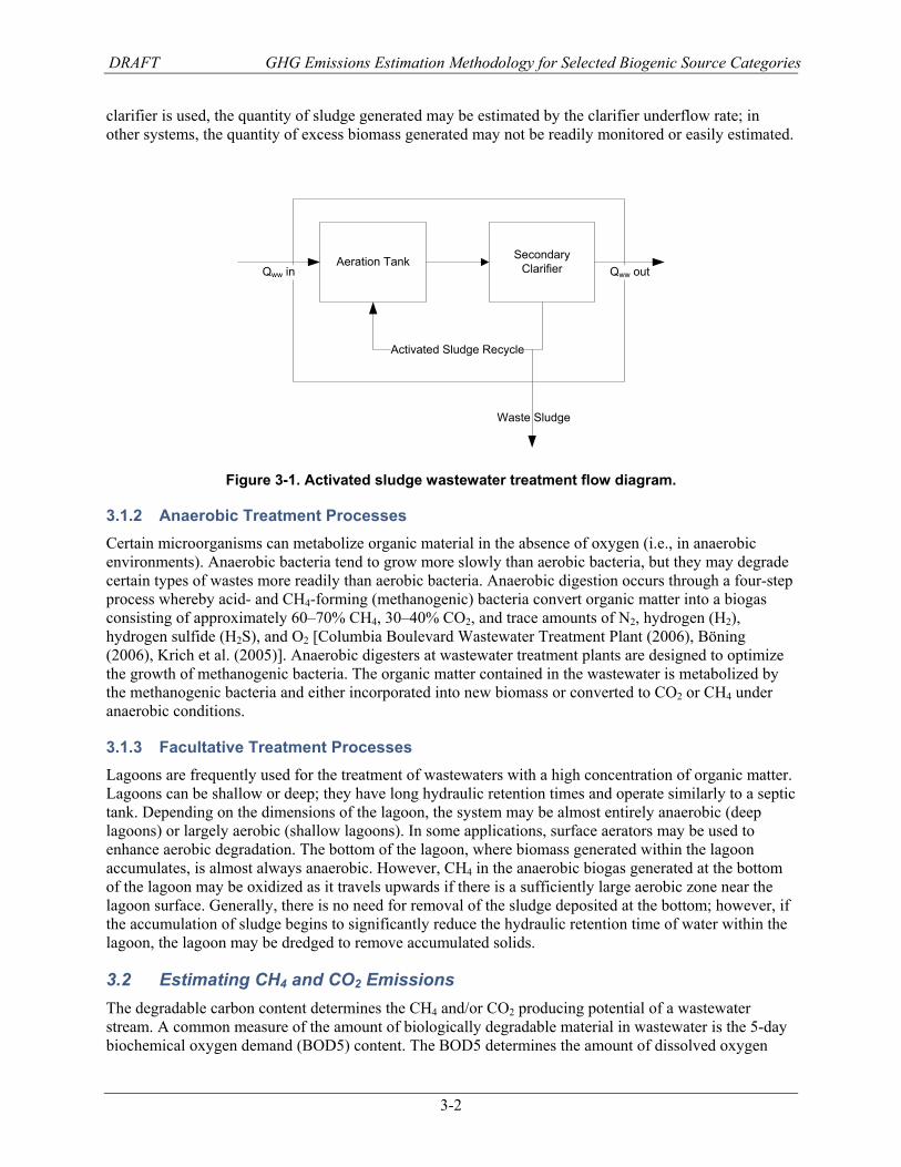
3.1.1 Aerobic Treatment Processes The activated sludge treatment process is one of the most commonly used biological wastewater treatment processes at both municipal and industrial wastewater treatment plants. There are many variations of activated sludge biological wastewater treatment processes, but they generally consist of two linked units: an aeration tank and a secondary clarifier. Oxygen is introduced into the aeration tank, either by diffused, submerged aeration or by surface aerators, to maintain the health of the microorganisms and ensure adequate oxidation of the organic compounds. A relatively high concentration of aerobic bacteria (“biomass”) is maintained in the aeration tank by settling out the aerobic bacteria in the secondary clarifier and recycling the majority of the biomass back to the aeration tank (Figure 3-1). A small amount of biomass is removed from the system (or “wasted”) to maintain the health of the biomass and maintain the desired biomass concentration in the aeration tank. The material balance around the system is simplified by considering the activated sludge process to be the combination of these two process units. There is a single influent wastewater flow to the aeration tank, and two effluent flows: the clarifier overflow and the wasted sludge stream. Neglecting minor losses, the clarifier overflow (or effluent) flow rate is equal to the influent flow rate. The wasted sludge is typically sent to either an aerobic or anaerobic digester, in which the bacteria feed upon themselves to reduce the quantity of biomass that requires ultimate disposal.
Some biological treatment units maintain high biomass concentrations without the use of clarifiers by providing high surface areas for biomass to grow on. These attached-growth or fixed-film systems include trickling filters and rotating biological contactors. Some of the biomass produced will eventually die or otherwise “slough off” from the support material and become entrained in the effluent. If a secondary
DRAFT GHG Emissions Estimation Methodology for Selected Biogenic Source Categories
3-2
clarifier is used, the quantity of sludge generated may be estimated by the clarifier underflow rate; in other systems, the quantity of excess biomass generated may not be readily monitored or easily estimated.
Aeration Tank Secondary Clarifier
Activated Sludge Recycle
Qww in Qww out
Waste Sludge
Figure 3-1. Activated sludge wastewater treatment flow diagram.
3.1.2 Anaerobic Treatment Processes Certain microorganisms can metabolize organic material in the absence of oxygen (i.e., in anaerobic environments). Anaerobic bacteria tend to grow more slowly than aerobic bacteria, but they may degrade certain types of wastes more readily than aerobic bacteria. Anaerobic digestion occurs through a four-step process whereby acid- and CH4-forming (methanogenic) bacteria convert organic matter into a biogas consisting of approximately 60–70% CH4, 30–40% CO2, and trace amounts of N2, hydrogen (H2), hydrogen sulfide (H2S), and O2 [Columbia Boulevard Wastewater Treatment Plant (2006), Böning (2006), Krich et al. (2005)]. Anaerobic digesters at wastewater treatment plants are designed to optimize the growth of methanogenic bacteria. The organic matter contained in the wastewater is metabolized by the methanogenic bacteria and either incorporated into new biomass or converted to CO2 or CH4 under anaerobic conditions.
3.1.3 Facultative Treatment Processes Lagoons are frequently used for the treatment of wastewaters with a high concentration of organic matter. Lagoons can be shallow or deep; they have long hydraulic retention times and operate similarly to a septic tank. Depending on the dimensions of the lagoon, the system may be almost entirely anaerobic (deep lagoons) or largely aerobic (shallow lagoons). In some applications, surface aerators may be used to enhance aerobic degradation. The bottom of the lagoon, where biomass generated within the lagoon accumulates, is almost always anaerobic. However, CH4 in the anaerobic biogas generated at the bottom of the lagoon may be oxidized as it travels upwards if there is a sufficiently large aerobic zone near the lagoon surface. Generally, there is no need for removal of the sludge deposited at the bottom; however, if the accumulation of sludge begins to significantly reduce the hydraulic retention time of water within the lagoon, the lagoon may be dredged to remove accumulated solids.
3.2 Estimating CH4 and CO2 Emissions The degradable carbon content determines the CH4 and/or CO2 producing potential of a wastewater stream. A common measure of the amount of biologically degradable material in wastewater is the 5-day biochemical oxygen demand (BOD5) content. The BOD5 determines the amount of dissolved oxygen
DRAFT GHG Emissions Estimation Methodology for Selected Biogenic Source Categories
3-3
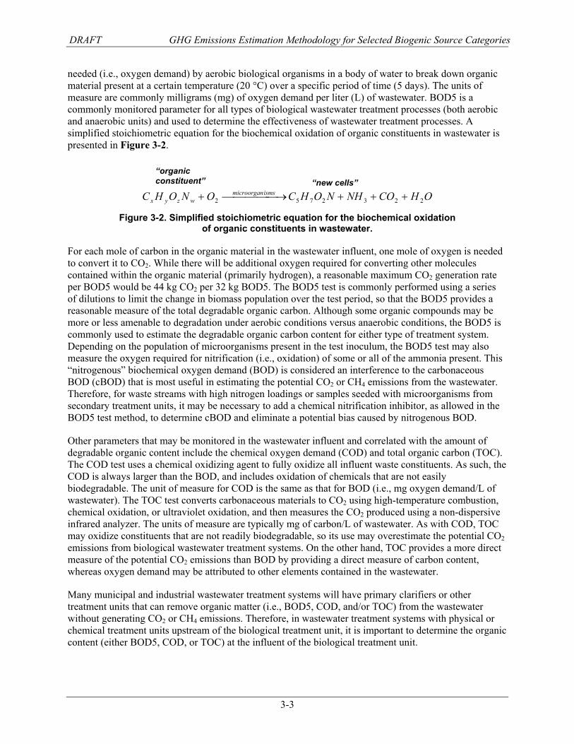
needed (i.e., oxygen demand) by aerobic biological organisms in a body of water to break down organic material present at a certain temperature (20 °C) over a specific period of time (5 days). The units of measure are commonly milligrams (mg) of oxygen demand per liter (L) of wastewater. BOD5 is a commonly monitored parameter for all types of biological wastewater treatment processes (both aerobic and anaerobic units) and used to determine the effectiveness of wastewater treatment processes. A simplified stoichiometric equation for the biochemical oxidation of organic constituents in wastewater is presented in Figure 3-2.
OHCONHNOHCONOHC ismsmicroorganwzyx 2232752 +++⎯⎯⎯⎯ →⎯+
Figure 3-2. Simplified stoichiometric equation for the biochemical oxidation of organic constituents in wastewater.
For each mole of carbon in the organic material in the wastewater influent, one mole of oxygen is needed to convert it to CO2. While there will be additional oxygen required for converting other molecules contained within the organic material (primarily hydrogen), a reasonable maximum CO2 generation rate per BOD5 would be 44 kg CO2 per 32 kg BOD5. The BOD5 test is commonly performed using a series of dilutions to limit the change in biomass population over the test period, so that the BOD5 provides a reasonable measure of the total degradable organic carbon. Although some organic compounds may be more or less amenable to degradation under aerobic conditions versus anaerobic conditions, the BOD5 is commonly used to estimate the degradable organic carbon content for either type of treatment system. Depending on the population of microorganisms present in the test inoculum, the BOD5 test may also measure the oxygen required for nitrification (i.e., oxidation) of some or all of the ammonia present. This “nitrogenous” biochemical oxygen demand (BOD) is considered an interference to the carbonaceous BOD (cBOD) that is most useful in estimating the potential CO2 or CH4 emissions from the wastewater. Therefore, for waste streams with high nitrogen loadings or samples seeded with microorganisms from secondary treatment units, it may be necessary to add a chemical nitrification inhibitor, as allowed in the BOD5 test method, to determine cBOD and eliminate a potential bias caused by nitrogenous BOD.
Other parameters that may be monitored in the wastewater influent and correlated with the amount of degradable organic content include the chemical oxygen demand (COD) and total organic carbon (TOC). The COD test uses a chemical oxidizing agent to fully oxidize all influent waste constituents. As such, the COD is always larger than the BOD, and includes oxidation of chemicals that are not easily biodegradable. The unit of measure for COD is the same as that for BOD (i.e., mg oxygen demand/L of wastewater). The TOC test converts carbonaceous materials to CO2 using high-temperature combustion, chemical oxidation, or ultraviolet oxidation, and then measures the CO2 produced using a non-dispersive infrared analyzer. The units of measure are typically mg of carbon/L of wastewater. As with COD, TOC may oxidize constituents that are not readily biodegradable, so its use may overestimate the potential CO2 emissions from biological wastewater treatment systems. On the other hand, TOC provides a more direct measure of the potential CO2 emissions than BOD by providing a direct measure of carbon content, whereas oxygen demand may be attributed to other elements contained in the wastewater.
Many municipal and industrial wastewater treatment systems will have primary clarifiers or other treatment units that can remove organic matter (i.e., BOD5, COD, and/or TOC) from the wastewater without generating CO2 or CH4 emissions. Therefore, in wastewater treatment systems with physical or chemical treatment units upstream of the biological treatment unit, it is important to determine the organic content (either BOD5, COD, or TOC) at the influent of the biological treatment unit.
“new cells” “organic constituent”
DRAFT GHG Emissions Estimation Methodology for Selected Biogenic Source Categories
3-4
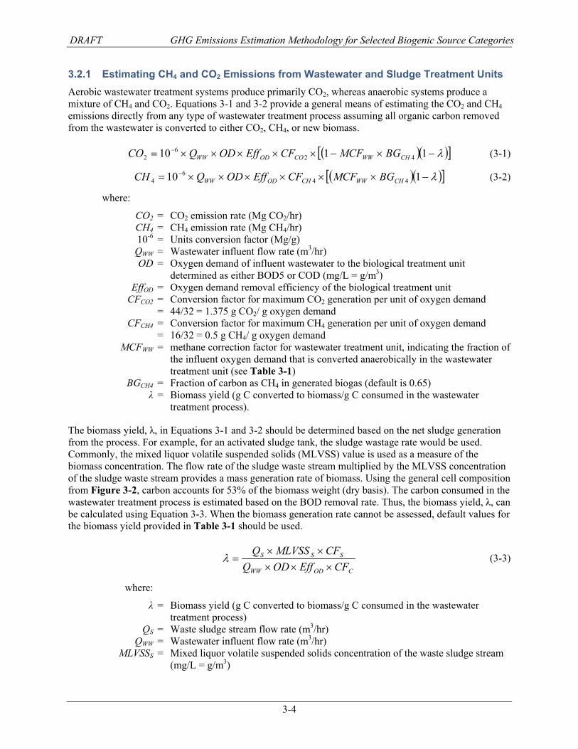
3.2.1 Estimating CH4 and CO2 Emissions from Wastewater and Sludge Treatment Units Aerobic wastewater treatment systems produce primarily CO2, whereas anaerobic systems produce a mixture of CH4 and CO2. Equations 3-1 and 3-2 provide a general means of estimating the CO2 and CH4 emissions directly from any type of wastewater treatment process assuming all organic carbon removed from the wastewater is converted to either CO2, CH4, or new biomass.
( )( )[ ]λ−×−×××××= − 1110 426
2 CHWWCOODWW BGMCFCFEffODQCO (3-1)
( )( )[ ]λ−××××××= − 110 446
4 CHWWCHODWW BGMCFCFEffODQCH (3-2)
where:
CO2 = CO2 emission rate (Mg CO2/hr) CH4 = CH4 emission rate (Mg CH4/hr) 10-6 = Units conversion factor (Mg/g) QWW = Wastewater influent flow rate (m3/hr) OD = Oxygen demand of influent wastewater to the biological treatment unit
determined as either BOD5 or COD (mg/L = g/m3) EffOD = Oxygen demand removal efficiency of the biological treatment unit CFCO2 = Conversion factor for maximum CO2 generation per unit of oxygen demand = 44/32 = 1.375 g CO2/ g oxygen demand CFCH4 = Conversion factor for maximum CH4 generation per unit of oxygen demand = 16/32 = 0.5 g CH4/ g oxygen demand MCFWW = methane correction factor for wastewater treatment unit, indicating the fraction of
the influent oxygen demand that is converted anaerobically in the wastewater treatment unit (see Table 3-1)
BGCH4 = Fraction of carbon as CH4 in generated biogas (default is 0.65) λ = Biomass yield (g C converted to biomass/g C consumed in the wastewater
treatment process).
The biomass yield, λ, in Equations 3-1 and 3-2 should be determined based on the net sludge generation from the process. For example, for an activated sludge tank, the sludge wastage rate would be used. Commonly, the mixed liquor volatile suspended solids (MLVSS) value is used as a measure of the biomass concentration. The flow rate of the sludge waste stream multiplied by the MLVSS concentration of the sludge waste stream provides a mass generation rate of biomass. Using the general cell composition from Figure 3-2, carbon accounts for 53% of the biomass weight (dry basis). The carbon consumed in the wastewater treatment process is estimated based on the BOD removal rate. Thus, the biomass yield, λ, can be calculated using Equation 3-3. When the biomass generation rate cannot be assessed, default values for the biomass yield provided in Table 3-1 should be used.
CODWW
SSS
CFEffODQCFMLVSSQ×××
××=λ (3-3)
where:
λ = Biomass yield (g C converted to biomass/g C consumed in the wastewater treatment process)
QS = Waste sludge stream flow rate (m3/hr) QWW = Wastewater influent flow rate (m3/hr) MLVSSS = Mixed liquor volatile suspended solids concentration of the waste sludge stream
(mg/L = g/m3)
DRAFT GHG Emissions Estimation Methodology for Selected Biogenic Source Categories
3-5
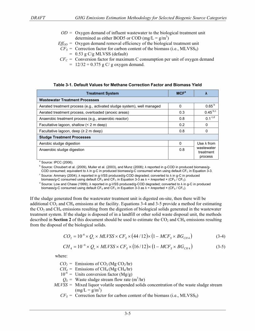
OD = Oxygen demand of influent wastewater to the biological treatment unit determined as either BOD5 or COD (mg/L = g/m3)
EffOD = Oxygen demand removal efficiency of the biological treatment unit CFS = Correction factor for carbon content of the biomass (i.e., MLVSSS) = 0.53 g C/g MLVSS (default) CFC = Conversion factor for maximum C consumption per unit of oxygen demand = 12/32 = 0.375 g C/ g oxygen demand.
Table 3-1. Default Values for Methane Correction Factor and Biomass Yield
Treatment System MCFa λ
Wastewater Treatment Processes Aerated treatment process (e.g., activated sludge system), well managed 0 0.65 b Aerated treatment process, overloaded (anoxic areas) 0.3 0.45 b,c Anaerobic treatment process (e.g., anaerobic reactor) 0.8 0.1 c,d Facultative lagoon, shallow (< 2 m deep) 0.2 0 Facultative lagoon, deep (≥ 2 m deep) 0.8 0 Sludge Treatment Processes Aerobic sludge digestion 0 Use λ from
wastewater treatment process
Anaerobic sludge digestion 0.8
a Source: IPCC (2006). b Source: Choubert et al. (2009), Muller et al. (2003), and Munz (2008); λ reported in g-COD in produced biomass/g-
COD consumed; equivalent to λ in g-C in produced biomass/g-C consumed when using default CFC in Equation 3-3. c Source: Ammary (2004); λ reported in g-VSS produced/g-COD degraded; converted to λ in g-C in produced
biomass/g-C consumed using default CFS and CFC in Equation 3-3 as λ = λreported × (CFS / CFC). d Source: Low and Chase (1999); λ reported in g-VSS produced/g-COD degraded; converted to λ in g-C in produced
biomass/g-C consumed using default CFS and CFC in Equation 3-3 as λ = λreported × (CFS / CFC).
If the sludge generated from the wastewater treatment unit is digested on-site, then there will be additional CO2 and CH4 emissions at the facility. Equations 3-4 and 3-5 provide a method for estimating the CO2 and CH4 emissions resulting from the digestion of biological solids generated in the wastewater treatment system. If the sludge is disposed of in a landfill or other solid waste disposal unit, the methods described in Section 2 of this document should be used to estimate the CO2 and CH4 emissions resulting from the disposal of the biological solids.
( ) ( )4-6
2 112/44 10 CHSSs BGMCFCFMLVSSQCO ×−×××××= (3-4)
( ) ( )46
4 112/1610 CHSSs BGMCFCFMLVSSQCH ×−×××××= − (3-5)
where:
CO2 = Emissions of CO2 (Mg CO2/hr) CH4 = Emissions of CH4 (Mg CH4/hr) 10-6 = Units conversion factor (Mg/g) QS = Waste sludge stream flow rate (m3/hr) MLVSS = Mixed liquor volatile suspended solids concentration of the waste sludge stream
(mg/L = g/m3) CFS = Correction factor for carbon content of the biomass (i.e., MLVSSS)
DRAFT GHG Emissions Estimation Methodology for Selected Biogenic Source Categories
3-6
= 0.53 g C/g MLVSS (default) MCFS = methane correction factor for sludge digestion, indicating the fraction of the
treated sludge that is converted anaerobically (see Table 3-1) BGCH4 = Fraction of carbon as CH4 in generated biogas (default is 0.65)
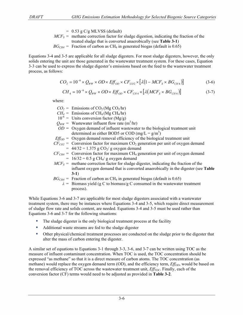
Equations 3-4 and 3-5 are applicable for all sludge digesters. For most sludge digesters, however, the only solids entering the unit are those generated in the wastewater treatment system. For these cases, Equation 3-3 can be used to express the sludge digester’s emissions based on the feed to the wastewater treatment process, as follows:
( )[ ]426
2 110 CHSCOODWW BGMCFCFEffODQCO ×−×××××= − λ (3-6)
( )[ ]446
4 10 CHSCHODWW BGMCFCFEffODQCH ××××××= − λ (3-7)
where:
CO2 = Emissions of CO2 (Mg CO2/hr) CH4 = Emissions of CH4 (Mg CH4/hr) 10-6 = Units conversion factor (Mg/g) QWW = Wastewater influent flow rate (m3/hr) OD = Oxygen demand of influent wastewater to the biological treatment unit
determined as either BOD5 or COD (mg/L = g/m3) EffOD = Oxygen demand removal efficiency of the biological treatment unit CFCO2 = Conversion factor for maximum CO2 generation per unit of oxygen demand = 44/32 = 1.375 g CO2/ g oxygen demand CFCH4 = Conversion factor for maximum CH4 generation per unit of oxygen demand = 16/32 = 0.5 g CH4/ g oxygen demand MCFS = methane correction factor for sludge digester, indicating the fraction of the
influent oxygen demand that is converted anaerobically in the digester (see Table 3-1)
BGCH4 = Fraction of carbon as CH4 in generated biogas (default is 0.65) λ = Biomass yield (g C to biomass/g C consumed in the wastewater treatment
process).
While Equations 3-6 and 3-7 are applicable for most sludge digesters associated with a wastewater treatment system, there may be instances where Equations 3-4 and 3-5, which require direct measurement of sludge flow rate and solids content, are needed. Equations 3-4 and 3-5 must be used rather than Equations 3-6 and 3-7 for the following situations:
The sludge digester is the only biological treatment process at the facility Additional waste streams are fed to the sludge digester Other physical/chemical treatment processes are conducted on the sludge prior to the digester that
alter the mass of carbon entering the digester.
A similar set of equations to Equations 3-1 through 3-3, 3-6, and 3-7 can be written using TOC as the measure of influent contaminant concentration. When TOC is used, the TOC concentration should be expressed “as methane” so that it is a direct measure of carbon atoms. The TOC concentration (as methane) would replace the oxygen demand term (OD), and the efficiency term, EffOD, would be based on the removal efficiency of TOC across the wastewater treatment unit, EffTOC. Finally, each of the conversion factor (CF) terms would need to be adjusted as provided in Table 3-2.
DRAFT GHG Emissions Estimation Methodology for Selected Biogenic Source Categories
3-7
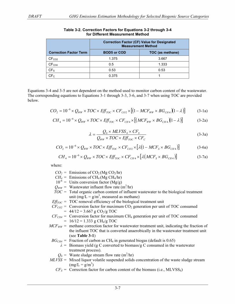
Table 3-2. Correction Factors for Equations 3-2 through 3-4 for Different Measurement Method
Correction Factor Term
Correction Factor (CF) Value for Designated Measurement Method
BOD5 or COD TOC (as methane)
CFCO2 1.375 3.667 CFCH4 0.5 1.333 CFS 0.53 0.53 CFC 0.375 1
Equations 3-4 and 3-5 are not dependent on the method used to monitor carbon content of the wastewater. The corresponding equations to Equations 3-1 through 3-3, 3-6, and 3-7 when using TOC are provided below.
( )( )[ ]λ−×−×××××= − 1110 426
2 CHWWCOTOCWW BGMCFCFEffTOCQCO (3-1a)
( )( )[ ]λ−××××××= − 110 446
4 CHWWCHTOCWW BGMCFCFEffTOCQCH (3-2a)
CTOCWW
SSS
CFEffTOCQCFMLVSSQ×××
××=λ (3-3a)
( )[ ]426
2 110 CHSCOTOCWW BGMCFCFEffTOCQCO ×−×××××= − λ (3-6a)
( )[ ]446
4 10 CHSCHTOCWW BGMCFCFEffTOCQCH ××××××= − λ (3-7a)
where:
CO2 = Emissions of CO2 (Mg CO2/hr) CH4 = Emissions of CH4 (Mg CH4/hr) 10-6 = Units conversion factor (Mg/g) QWW = Wastewater influent flow rate (m3/hr) TOC = Total organic carbon content of influent wastewater to the biological treatment
unit (mg/L = g/m3, measured as methane) EffTOC = TOC removal efficiency of the biological treatment unit CFCO2 = Conversion factor for maximum CO2 generation per unit of TOC consumed = 44/12 = 3.667 g CO2/g TOC CFCH4 = Conversion factor for maximum CH4 generation per unit of TOC consumed = 16/12 = 1.333 g CH4/g TOC MCFWW = methane correction factor for wastewater treatment unit, indicating the fraction of
the influent TOC that is converted anaerobically in the wastewater treatment unit (see Table 3-1)
BGCH4 = Fraction of carbon as CH4 in generated biogas (default is 0.65) λ = Biomass yield (g C converted to biomass/g C consumed in the wastewater
treatment process). QS = Waste sludge stream flow rate (m3/hr) MLVSS = Mixed liquor volatile suspended solids concentration of the waste sludge stream
(mg/L = g/m3) CFS = Correction factor for carbon content of the biomass (i.e., MLVSSS)
DRAFT GHG Emissions Estimation Methodology for Selected Biogenic Source Categories
3-8
= 0.53 g C/g MLVSS (default) CFC = Conversion factor for maximum C consumption per unit of TOC consumed = 12/12 = 1.0 g C/g TOC MCFS = methane correction factor for sludge digester, indicating the fraction of the
influent TOC that is converted anaerobically in the digester (see Table 3-1)
If measurement data are available on a daily or hourly basis, the emissions for each hour or day can be calculated and all the values for the year summed to calculate the annual emissions, and the largest short-term emissions rate can be used to calculate or estimate the worst-case hourly emissions rate. When these measurement data are not available, typical or average flow rates and concentrations should be used along with the annual operating hours to calculate the annual average emissions. To estimate the hourly emission rate when frequent measurement data are not available, the maximum anticipated flow rate (or wastewater treatment system capacity) and highest anticipated organic load (as BOD, COD, or TOC) to the system should be used.
DRAFT GHG Emissions Estimation Methodology for Selected Biogenic Source Categories
3-9
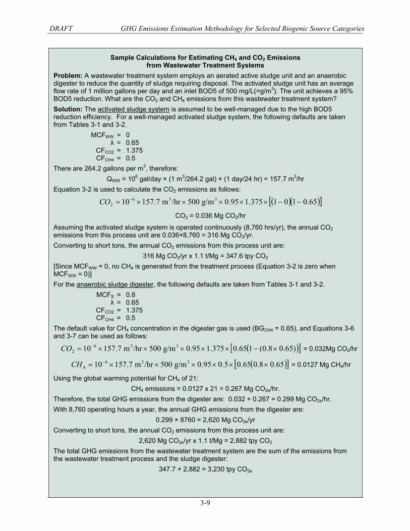
Sample Calculations for Estimating CH4 and CO2 Emissions from Wastewater Treatment Systems
Problem: A wastewater treatment system employs an aerated active sludge unit and an anaerobic digester to reduce the quantity of sludge requiring disposal. The activated sludge unit has an average flow rate of 1 million gallons per day and an inlet BOD5 of 500 mg/L(=g/m3). The unit achieves a 95% BOD5 reduction. What are the CO2 and CH4 emissions from this wastewater treatment system? Solution: The activated sludge system is assumed to be well-managed due to the high BOD5 reduction efficiency. For a well-managed activated sludge system, the following defaults are taken from Tables 3-1 and 3-2. MCFWW = 0 λ = 0.65 CFCO2 = 1.375 CFCH4 = 0.5 There are 264.2 gallons per m3, therefore:
QWW = 106 gal/day × (1 m3/264.2 gal) × (1 day/24 hr) = 157.7 m3/hr Equation 3-2 is used to calculate the CO2 emissions as follows:
( )( )[ ]65.0101375.195.0g/m500/hrm7.15710 3362 −−×××××= −CO
CO2 = 0.036 Mg CO2/hr
Assuming the activated sludge system is operated continuously (8,760 hrs/yr), the annual CO2 emissions from this process unit are 0.036×8,760 = 316 Mg CO2/yr. Converting to short tons, the annual CO2 emissions from this process unit are:
316 Mg CO2/yr x 1.1 t/Mg = 347.6 tpy CO2 [Since MCFWW = 0, no CH4 is generated from the treatment process (Equation 3-2 is zero when MCFWW = 0)] For the anaerobic sludge digester, the following defaults are taken from Tables 3-1 and 3-2. MCFS = 0.8 λ = 0.65 CFCO2 = 1.375 CFCH4 = 0.5 The default value for CH4 concentration in the digester gas is used (BGCH4 = 0.65), and Equations 3-6 and 3-7 can be used as follows:
( )[ ])65.08.0(165.0375.195.0g/m500/hrm7.15710 3362 ×−×××××= −CO = 0.032Mg CO2/hr
( )[ ]65.08.065.05.095.0g/m500/hrm7.15710 3364 ××××××= −CH = 0.0127 Mg CH4/hr
Using the global warming potential for CH4 of 21: CH4 emissions = 0.0127 x 21 = 0.267 Mg CO2e/hr.
Therefore, the total GHG emissions from the digester are: 0.032 + 0.267 = 0.299 Mg CO2e/hr. With 8,760 operating hours a year, the annual GHG emissions from the digester are:
0.299 × 8760 = 2,620 Mg CO2e/yr Converting to short tons, the annual CO2 emissions from this process unit are:
2,620 Mg CO2e/yr x 1.1 t/Mg = 2,882 tpy CO2 The total GHG emissions from the wastewater treatment system are the sum of the emissions from the wastewater treatment process and the sludge digester:
347.7 + 2,882 = 3,230 tpy CO2e
DRAFT GHG Emissions Estimation Methodology for Selected Biogenic Source Categories
3-10
3.2.2 Estimating CH4 and CO2 Emissions from Combustion of Biogas If the CH4 generated by anaerobic wastewater treatment process or anaerobic sludge digestion process is captured and combusted (in a flare or other combustion device), then there will be a conversion of CH4 to CO2 in the biogas combustion unit. The methods for calculating the CO2 and CH4 emissions based on measurement of the volume and CH4 concentration of the biogas are presented in Section 2.1.3 of this document.
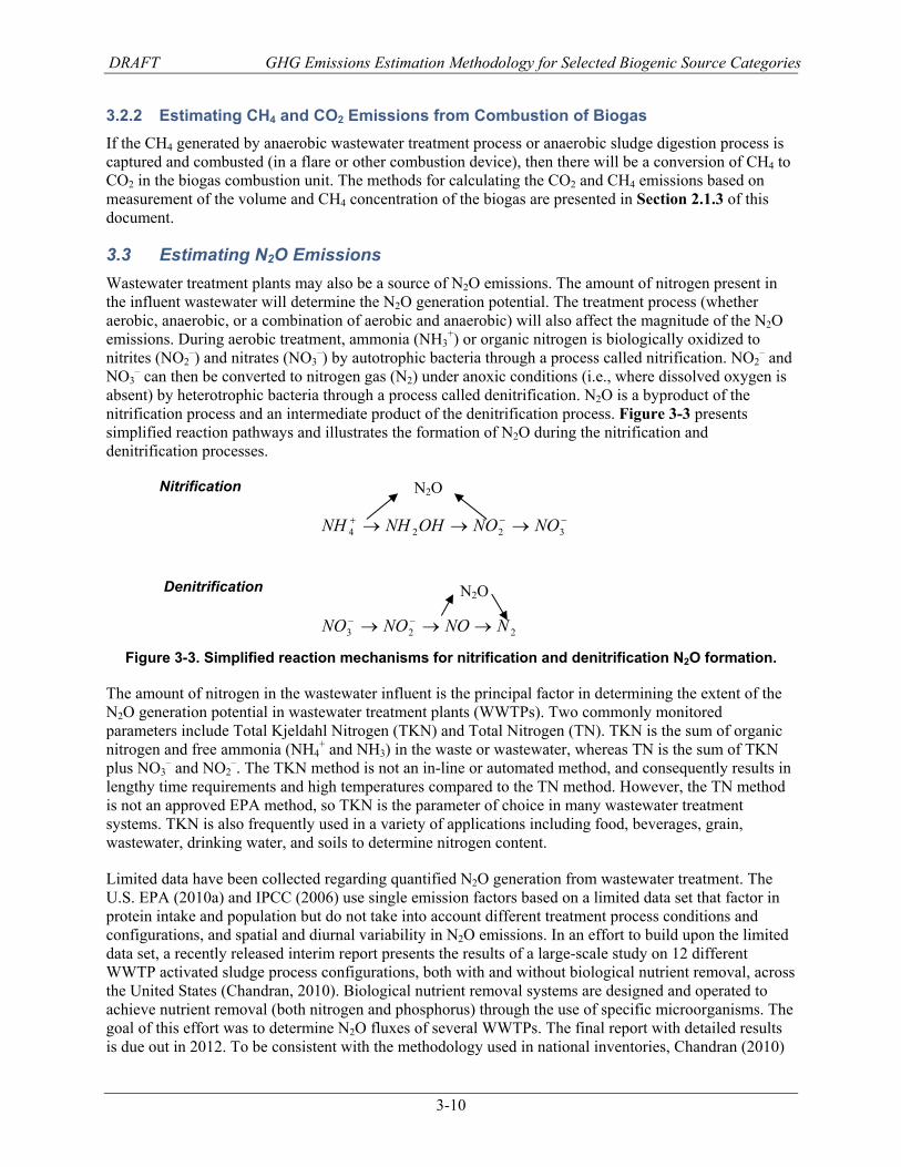
3.3 Estimating N2O Emissions Wastewater treatment plants may also be a source of N2O emissions. The amount of nitrogen present in the influent wastewater will determine the N2O generation potential. The treatment process (whether aerobic, anaerobic, or a combination of aerobic and anaerobic) will also affect the magnitude of the N2O emissions. During aerobic treatment, ammonia (NH3
+) or organic nitrogen is biologically oxidized to nitrites (NO2
–) and nitrates (NO3–) by autotrophic bacteria through a process called nitrification. NO2
– and NO3
– can then be converted to nitrogen gas (N2) under anoxic conditions (i.e., where dissolved oxygen is absent) by heterotrophic bacteria through a process called denitrification. N2O is a byproduct of the nitrification process and an intermediate product of the denitrification process. Figure 3-3 presents simplified reaction pathways and illustrates the formation of N2O during the nitrification and denitrification processes.
Nitrification
−−+ →→→ 3224 NONOOHNHNH
Denitrification
223 NNONONO →→→ −−
Figure 3-3. Simplified reaction mechanisms for nitrification and denitrification N2O formation.
The amount of nitrogen in the wastewater influent is the principal factor in determining the extent of the N2O generation potential in wastewater treatment plants (WWTPs). Two commonly monitored parameters include Total Kjeldahl Nitrogen (TKN) and Total Nitrogen (TN). TKN is the sum of organic nitrogen and free ammonia (NH4
+ and NH3) in the waste or wastewater, whereas TN is the sum of TKN plus NO3
– and NO2–. The TKN method is not an in-line or automated method, and consequently results in
lengthy time requirements and high temperatures compared to the TN method. However, the TN method is not an approved EPA method, so TKN is the parameter of choice in many wastewater treatment systems. TKN is also frequently used in a variety of applications including food, beverages, grain, wastewater, drinking water, and soils to determine nitrogen content.
Limited data have been collected regarding quantified N2O generation from wastewater treatment. The U.S. EPA (2010a) and IPCC (2006) use single emission factors based on a limited data set that factor in protein intake and population but do not take into account different treatment process conditions and configurations, and spatial and diurnal variability in N2O emissions. In an effort to build upon the limited data set, a recently released interim report presents the results of a large-scale study on 12 different WWTP activated sludge process configurations, both with and without biological nutrient removal, across the United States (Chandran, 2010). Biological nutrient removal systems are designed and operated to achieve nutrient removal (both nitrogen and phosphorus) through the use of specific microorganisms. The goal of this effort was to determine N2O fluxes of several WWTPs. The final report with detailed results is due out in 2012. To be consistent with the methodology used in national inventories, Chandran (2010)
N2O
N2O
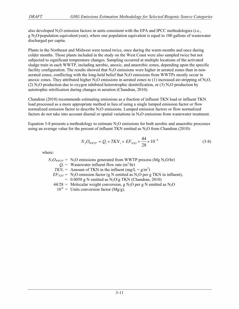
DRAFT GHG Emissions Estimation Methodology for Selected Biogenic Source Categories
3-11
also developed N2O emission factors in units consistent with the EPA and IPCC methodologies (i.e., g N2O/population equivalent/year), where one population equivalent is equal to 100 gallons of wastewater discharged per capita.
Plants in the Northeast and Midwest were tested twice, once during the warm months and once during colder months. Those plants included in the study on the West Coast were also sampled twice but not subjected to significant temperature changes. Sampling occurred at multiple locations of the activated sludge train in each WWTP, including aerobic, anoxic, and anaerobic zones, depending upon the specific facility configuration. The results showed that N2O emissions were higher in aerated zones than in non-aerated zones, conflicting with the long-held belief that N2O emissions from WWTPs mostly occur in anoxic zones. They attributed higher N2O emissions in aerated zones to (1) increased air-stripping of N2O, (2) N2O production due to oxygen inhibited heterotrophic denitrification, or (3) N2O production by autotrophic nitrification during changes in aeration (Chandran, 2010).
Chandran (2010) recommends estimating emissions as a fraction of influent TKN load or influent TKN load processed as a more appropriate method in lieu of using a single lumped emission factor or flow normalized emission factor to describe N2O emissions. Lumped emission factors or flow normalized factors do not take into account diurnal or spatial variations in N2O emissions from wastewater treatment.
Equation 3-8 presents a methodology to estimate N2O emissions for both aerobic and anaerobic processes using an average value for the percent of influent TKN emitted as N2O from Chandran (2010):
6N2O2 10
2844 −××××= EFTKNQON iiWWTP (3-8)
where:
N2OWWTP = N2O emissions generated from WWTP process (Mg N2O/hr) Qi = Wastewater influent flow rate (m3/hr) TKNi = Amount of TKN in the influent (mg/L = g/m3) EFN2O = N2O emission factor (g N emitted as N2O per g TKN in influent), = 0.0050 g N emitted as N2O/g TKN (Chandran, 2010) 44/28 = Molecular weight conversion, g N2O per g N emitted as N2O 10-6 = Units conversion factor (Mg/g).
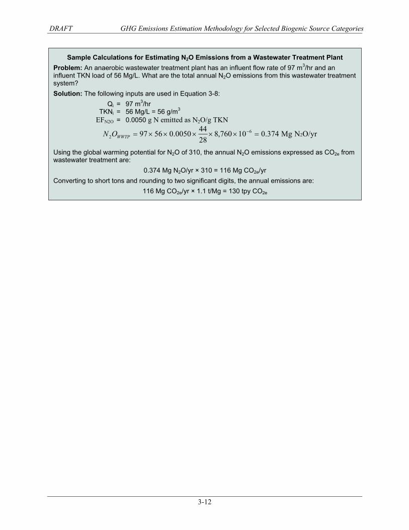
DRAFT GHG Emissions Estimation Methodology for Selected Biogenic Source Categories
3-12
Sample Calculations for Estimating N2O Emissions from a Wastewater Treatment Plant Problem: An anaerobic wastewater treatment plant has an influent flow rate of 97 m3/hr and an influent TKN load of 56 Mg/L. What are the total annual N2O emissions from this wastewater treatment system? Solution: The following inputs are used in Equation 3-8: Qi = 97 m3/hr TKNi = 56 Mg/L = 56 g/m3 EFN2O = 0.0050 g N emitted as N2O/g TKN
O/yrN Mg374.010760,828440050.05697 2
62 =×××××= −
WWTPON
Using the global warming potential for N2O of 310, the annual N2O emissions expressed as CO2e from wastewater treatment are:
0.374 Mg N2O/yr × 310 = 116 Mg CO2e/yr Converting to short tons and rounding to two significant digits, the annual emissions are:
116 Mg CO2e/yr × 1.1 t/Mg = 130 tpy CO2e
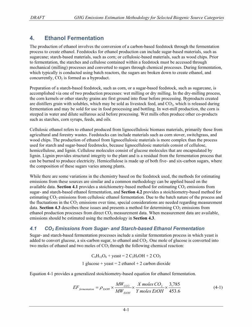
DRAFT GHG Emissions Estimation Methodology for Selected Biogenic Source Categories
4-1
4. Ethanol Fermentation The production of ethanol involves the conversion of a carbon-based feedstock through the fermentation process to create ethanol. Feedstocks for ethanol production can include sugar-based materials, such as sugarcane; starch-based materials, such as corn; or cellulosic-based materials, such as wood chips. Prior to fermentation, the starches and cellulose contained within a feedstock must be accessed through mechanical (milling) processes and converted to sugars through chemical processes. During fermentation, which typically is conducted using batch reactors, the sugars are broken down to create ethanol, and concurrently, CO2 is formed as a byproduct.
Preparation of a starch-based feedstock, such as corn, or a sugar-based feedstock, such as sugarcane, is accomplished via one of two production processes: wet milling or dry milling. In the dry-milling process, the corn kernels or other starchy grains are first ground into flour before processing. Byproducts created are distillers grain with solubles, which may be sold as livestock feed, and CO2, which is released during fermentation and may be sold for use in food processing and bottling. In wet-mill production, the corn is steeped in water and dilute sulfurous acid before processing. Wet mills often produce other co-products such as starches, corn syrups, feeds, and oils.
Cellulosic ethanol refers to ethanol produced from lignocellulosic biomass materials, primarily those from agricultural and forestry wastes. Feedstocks can include materials such as corn stover, switchgrass, and wood chips. The production of ethanol from lignocellulosic materials is more complex than the process used for starch and sugar-based feedstocks, because lignocellulosic materials consist of cellulose, hemicellulose, and lignin. Cellulose molecules consist of glucose molecules that are encapsulated by lignin. Lignin provides structural integrity to the plant and is a residual from the fermentation process that can be burned to produce electricity. Hemicellulose is made up of both five- and six-carbon sugars, where the composition of these sugars varies among plants.
While there are some variations in the chemistry based on the feedstock used, the methods for estimating emissions from these sources are similar and a common methodology can be applied based on the available data. Section 4.1 provides a stoichiometry-based method for estimating CO2 emissions from sugar- and starch-based ethanol fermentation, and Section 4.2 provides a stoichiometry-based method for estimating CO2 emissions from cellulosic ethanol fermentation. Due to the batch nature of the process and the fluctuations in the CO2 emissions over time, special considerations are needed regarding measurement data. Section 4.3 describes these issues and presents a method for determining CO2 emissions from ethanol production processes from direct CO2 measurement data. When measurement data are available, emissions should be estimated using the methodology in Section 4.3.
4.1 CO2 Emissions from Sugar- and Starch-based Ethanol Fermentation Sugar- and starch-based fermentation processes include a similar fermentation process in which yeast is added to convert glucose, a six-carbon sugar, to ethanol and CO2. One mole of glucose is converted into two moles of ethanol and two moles of CO2 through the following chemical reaction:
C6H12O6 + yeast = 2 C2H5OH + 2 CO2
1 glucose + yeast = 2 ethanol + 2 carbon dioxide
Equation 4-1 provides a generalized stoichiometry-based equation for ethanol fermentation.
6.453
785,322 ×××=EtOHmolesYCOmolesX
MWMWEF
EtOH
COEtOHonfermentati ρ (4-1)
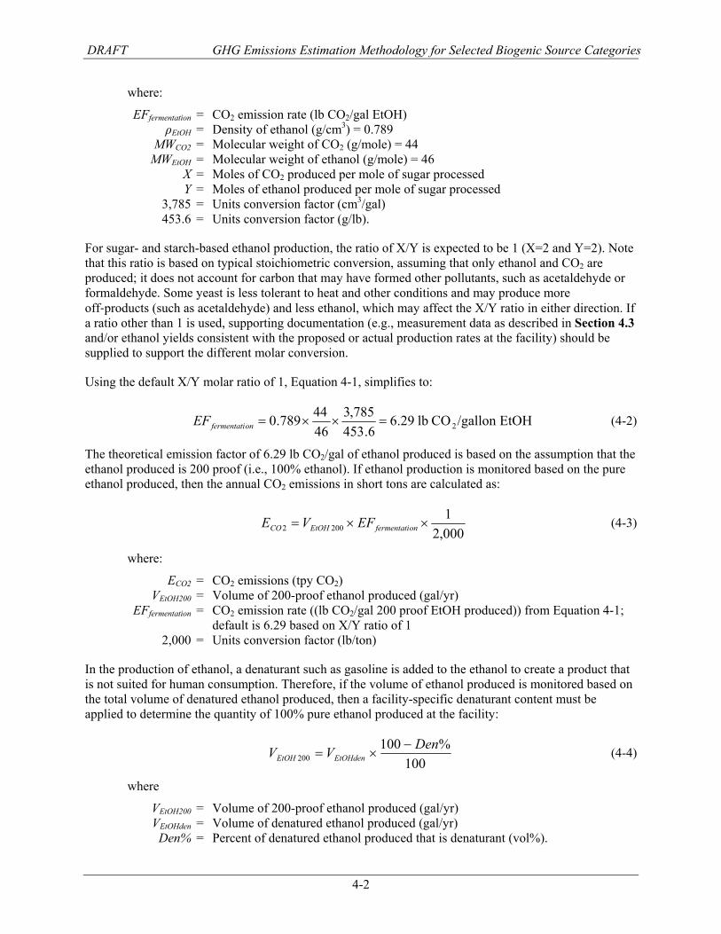
DRAFT GHG Emissions Estimation Methodology for Selected Biogenic Source Categories
4-2
where:
EFfermentation = CO2 emission rate (lb CO2/gal EtOH) ρEtOH = Density of ethanol (g/cm3) = 0.789 MWCO2 = Molecular weight of CO2 (g/mole) = 44 MWEtOH = Molecular weight of ethanol (g/mole) = 46 X = Moles of CO2 produced per mole of sugar processed Y = Moles of ethanol produced per mole of sugar processed 3,785 = Units conversion factor (cm3/gal) 453.6 = Units conversion factor (g/lb).
For sugar- and starch-based ethanol production, the ratio of X/Y is expected to be 1 (X=2 and Y=2). Note that this ratio is based on typical stoichiometric conversion, assuming that only ethanol and CO2 are produced; it does not account for carbon that may have formed other pollutants, such as acetaldehyde or formaldehyde. Some yeast is less tolerant to heat and other conditions and may produce more off‐products (such as acetaldehyde) and less ethanol, which may affect the X/Y ratio in either direction. If a ratio other than 1 is used, supporting documentation (e.g., measurement data as described in Section 4.3 and/or ethanol yields consistent with the proposed or actual production rates at the facility) should be supplied to support the different molar conversion.
Using the default X/Y molar ratio of 1, Equation 4-1, simplifies to:
EtOH/gallon COlb29.66.453
785,34644789.0 2=××=onfermentatiEF (4-2)
The theoretical emission factor of 6.29 lb CO2/gal of ethanol produced is based on the assumption that the ethanol produced is 200 proof (i.e., 100% ethanol). If ethanol production is monitored based on the pure ethanol produced, then the annual CO2 emissions in short tons are calculated as:
000,21
2002 ××= onfermentatiEtOHCO EFVE (4-3)
where:
ECO2 = CO2 emissions (tpy CO2) VEtOH200 = Volume of 200-proof ethanol produced (gal/yr) EFfermentation = CO2 emission rate ((lb CO2/gal 200 proof EtOH produced)) from Equation 4-1;
default is 6.29 based on X/Y ratio of 1 2,000 = Units conversion factor (lb/ton)
In the production of ethanol, a denaturant such as gasoline is added to the ethanol to create a product that is not suited for human consumption. Therefore, if the volume of ethanol produced is monitored based on the total volume of denatured ethanol produced, then a facility-specific denaturant content must be applied to determine the quantity of 100% pure ethanol produced at the facility:
100
%100200
DenVV EtOHdenEtOH−
×= (4-4)
where
VEtOH200 = Volume of 200-proof ethanol produced (gal/yr) VEtOHden = Volume of denatured ethanol produced (gal/yr) Den% = Percent of denatured ethanol produced that is denaturant (vol%).
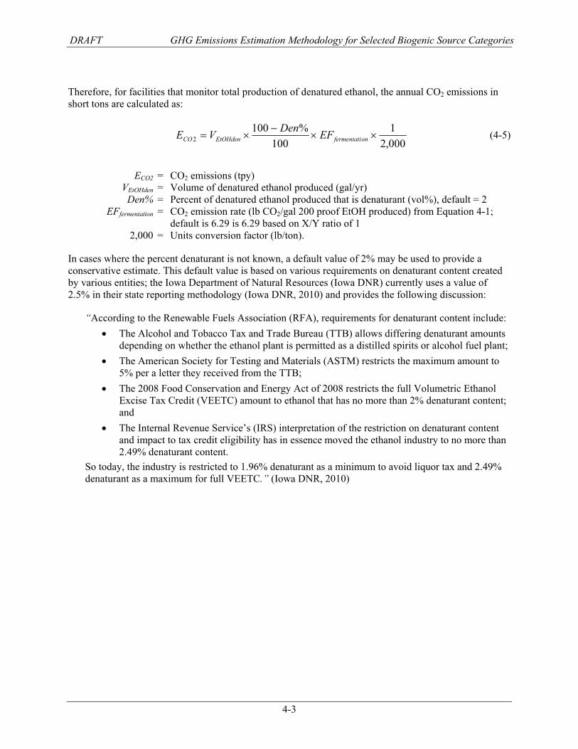
DRAFT GHG Emissions Estimation Methodology for Selected Biogenic Source Categories
4-3
Therefore, for facilities that monitor total production of denatured ethanol, the annual CO2 emissions in short tons are calculated as:
000,21
100%100
2 ××−
×= onfermentatiEtOHdenCO EFDenVE (4-5)
ECO2 = CO2 emissions (tpy) VEtOHden = Volume of denatured ethanol produced (gal/yr) Den% = Percent of denatured ethanol produced that is denaturant (vol%), default = 2 EFfermentation = CO2 emission rate (lb CO2/gal 200 proof EtOH produced) from Equation 4-1;
default is 6.29 is 6.29 based on X/Y ratio of 1 2,000 = Units conversion factor (lb/ton).
In cases where the percent denaturant is not known, a default value of 2% may be used to provide a conservative estimate. This default value is based on various requirements on denaturant content created by various entities; the Iowa Department of Natural Resources (Iowa DNR) currently uses a value of 2.5% in their state reporting methodology (Iowa DNR, 2010) and provides the following discussion:
“According to the Renewable Fuels Association (RFA), requirements for denaturant content include: • The Alcohol and Tobacco Tax and Trade Bureau (TTB) allows differing denaturant amounts
depending on whether the ethanol plant is permitted as a distilled spirits or alcohol fuel plant; • The American Society for Testing and Materials (ASTM) restricts the maximum amount to
5% per a letter they received from the TTB; • The 2008 Food Conservation and Energy Act of 2008 restricts the full Volumetric Ethanol
Excise Tax Credit (VEETC) amount to ethanol that has no more than 2% denaturant content; and
• The Internal Revenue Service’s (IRS) interpretation of the restriction on denaturant content and impact to tax credit eligibility has in essence moved the ethanol industry to no more than 2.49% denaturant content.
So today, the industry is restricted to 1.96% denaturant as a minimum to avoid liquor tax and 2.49% denaturant as a maximum for full VEETC.” (Iowa DNR, 2010)
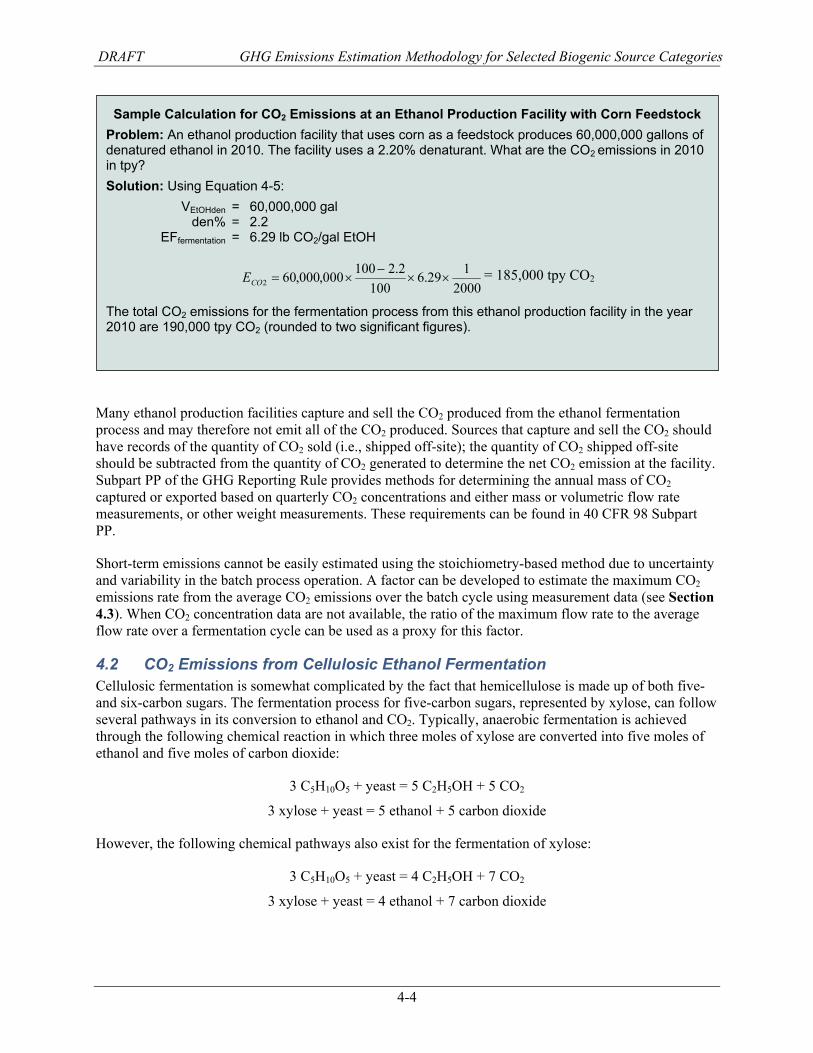
DRAFT GHG Emissions Estimation Methodology for Selected Biogenic Source Categories
4-4
Many ethanol production facilities capture and sell the CO2 produced from the ethanol fermentation process and may therefore not emit all of the CO2 produced. Sources that capture and sell the CO2 should have records of the quantity of CO2 sold (i.e., shipped off-site); the quantity of CO2 shipped off-site should be subtracted from the quantity of CO2 generated to determine the net CO2 emission at the facility. Subpart PP of the GHG Reporting Rule provides methods for determining the annual mass of CO2 captured or exported based on quarterly CO2 concentrations and either mass or volumetric flow rate measurements, or other weight measurements. These requirements can be found in 40 CFR 98 Subpart PP.
Short-term emissions cannot be easily estimated using the stoichiometry-based method due to uncertainty and variability in the batch process operation. A factor can be developed to estimate the maximum CO2 emissions rate from the average CO2 emissions over the batch cycle using measurement data (see Section 4.3). When CO2 concentration data are not available, the ratio of the maximum flow rate to the average flow rate over a fermentation cycle can be used as a proxy for this factor.
4.2 CO2 Emissions from Cellulosic Ethanol Fermentation Cellulosic fermentation is somewhat complicated by the fact that hemicellulose is made up of both five- and six-carbon sugars. The fermentation process for five-carbon sugars, represented by xylose, can follow several pathways in its conversion to ethanol and CO2. Typically, anaerobic fermentation is achieved through the following chemical reaction in which three moles of xylose are converted into five moles of ethanol and five moles of carbon dioxide:
3 C5H10O5 + yeast = 5 C2H5OH + 5 CO2
3 xylose + yeast = 5 ethanol + 5 carbon dioxide
However, the following chemical pathways also exist for the fermentation of xylose:
3 C5H10O5 + yeast = 4 C2H5OH + 7 CO2
3 xylose + yeast = 4 ethanol + 7 carbon dioxide
Sample Calculation for CO2 Emissions at an Ethanol Production Facility with Corn Feedstock Problem: An ethanol production facility that uses corn as a feedstock produces 60,000,000 gallons of denatured ethanol in 2010. The facility uses a 2.20% denaturant. What are the CO2 emissions in 2010 in tpy? Solution: Using Equation 4-5: VEtOHden = 60,000,000 gal den% = 2.2 EFfermentation = 6.29 lb CO2/gal EtOH
2000
129.6100
2.2100000,000,602 ××−
×=COE = 185,000 tpy CO2
The total CO2 emissions for the fermentation process from this ethanol production facility in the year 2010 are 190,000 tpy CO2 (rounded to two significant figures).
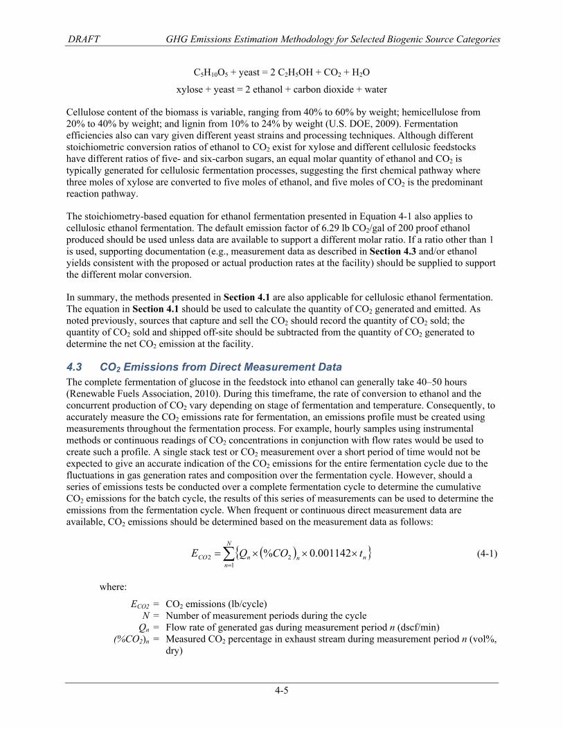
DRAFT GHG Emissions Estimation Methodology for Selected Biogenic Source Categories
4-5
C5H10O5 + yeast = 2 C2H5OH + CO2 + H2O
xylose + yeast = 2 ethanol + carbon dioxide + water
Cellulose content of the biomass is variable, ranging from 40% to 60% by weight; hemicellulose from 20% to 40% by weight; and lignin from 10% to 24% by weight (U.S. DOE, 2009). Fermentation efficiencies also can vary given different yeast strains and processing techniques. Although different stoichiometric conversion ratios of ethanol to CO2 exist for xylose and different cellulosic feedstocks have different ratios of five- and six-carbon sugars, an equal molar quantity of ethanol and CO2 is typically generated for cellulosic fermentation processes, suggesting the first chemical pathway where three moles of xylose are converted to five moles of ethanol, and five moles of CO2 is the predominant reaction pathway.
The stoichiometry-based equation for ethanol fermentation presented in Equation 4-1 also applies to cellulosic ethanol fermentation. The default emission factor of 6.29 lb CO2/gal of 200 proof ethanol produced should be used unless data are available to support a different molar ratio. If a ratio other than 1 is used, supporting documentation (e.g., measurement data as described in Section 4.3 and/or ethanol yields consistent with the proposed or actual production rates at the facility) should be supplied to support the different molar conversion.
In summary, the methods presented in Section 4.1 are also applicable for cellulosic ethanol fermentation. The equation in Section 4.1 should be used to calculate the quantity of CO2 generated and emitted. As noted previously, sources that capture and sell the CO2 should record the quantity of CO2 sold; the quantity of CO2 sold and shipped off-site should be subtracted from the quantity of CO2 generated to determine the net CO2 emission at the facility.
4.3 CO2 Emissions from Direct Measurement Data The complete fermentation of glucose in the feedstock into ethanol can generally take 40–50 hours (Renewable Fuels Association, 2010). During this timeframe, the rate of conversion to ethanol and the concurrent production of CO2 vary depending on stage of fermentation and temperature. Consequently, to accurately measure the CO2 emissions rate for fermentation, an emissions profile must be created using measurements throughout the fermentation process. For example, hourly samples using instrumental methods or continuous readings of CO2 concentrations in conjunction with flow rates would be used to create such a profile. A single stack test or CO2 measurement over a short period of time would not be expected to give an accurate indication of the CO2 emissions for the entire fermentation cycle due to the fluctuations in gas generation rates and composition over the fermentation cycle. However, should a series of emissions tests be conducted over a complete fermentation cycle to determine the cumulative CO2 emissions for the batch cycle, the results of this series of measurements can be used to determine the emissions from the fermentation cycle. When frequent or continuous direct measurement data are available, CO2 emissions should be determined based on the measurement data as follows:
( ){ }∑=
×××=N
nnnnCO tCOQE
122 001142.0% (4-1)
where:
ECO2 = CO2 emissions (lb/cycle) N = Number of measurement periods during the cycle Qn = Flow rate of generated gas during measurement period n (dscf/min) (%CO2)n = Measured CO2 percentage in exhaust stream during measurement period n (vol%,
dry)
DRAFT GHG Emissions Estimation Methodology for Selected Biogenic Source Categories
4-6
0.001142 = Units conversion factor for CO2 (lb CO2/dscf per vol% CO2); uses 68°F and 1 atmosphere as standard conditions
tn = Time interval associated with measurement period n (min).
The emissions from each batch processed can be calculated using Equation 4-1, and these values can be summed to calculate the annual emissions from the ethanol production process. If measurement data are available for only one cycle, a site-specific emission factor (lb CO2 emitted/ gal EtOH produced) can be developed for that cycle and used rather than the stoichiometry-based emission factor in Equation 4-1 or default emission factor from Equation 4-2. Individual measurement period data can also be evaluated to determine the maximum hourly emission rate during the fermentation cycle. This value can be used directly if the measurement is made during maximum ethanol production. Otherwise, the data can be used to develop a ratio of the maximum CO2 emission rate to the average CO2 emissions rate over the cycle. The maximum hourly rate can then be estimated based on the average CO2 emissions (from Section 4.1) at maximum ethanol production rates.
DRAFT GHG Emissions Estimation Methodology for Selected Biogenic Source Categories
5-1
5. References Ammary, B.Y. 2004. Nutrient requirements in biological industrial wastewater treatment. African Journal
of Biotechnology 3(4):236–238.
Barlaz, M.A. 1998. Carbon storage during biodegradation of municipal solid waste components in laboratory-scale landfills. Global Biogeochemical Cycles 12(2):373–380.
Böning, Rainer. 2006. Presentation entitled: Producing and Using Digester Gas at a Wastewater Treatment Plant. December 5. Available at http://www.erftverband.de/digester-gas.pdf
Chandran, K. 2010. Greenhouse Nitrogen Emission from Wastewater Treatment Operations: Interim Report. Water Environment Research Foundation (WERF), Report Number U4R07a.
Choubert, J-M., A. Marquot, A-E. Stricker, Y. Racault, S. Gillot, and A. Héduit. 2009. Anoxic and aerobic values for the yield coefficient of the heterotrophic biomass: determination at full-scale plants and consequences on simulations. Water SA 35(1):103–109.
Columbia Boulevard Wastewater Treatment Plant, Portland, OR. 2006. Presentation entitled: Energy Management Using Microturbine Technology. September. Available at http://www.naseo.org/committees/energyproduction/documents/Energy_Management_Using_Microturbine_Technology.pdf
Das, K.C., E.W. Tollner, and T.G. Tornabene. 1998. Composting pulp and paper industry wastes: process design and product evaluation. In Compost in the Southeast: Proceedings of the 1998 Conference. Athens, GA. Pp. 129–123. Available at http://www.p2pays.org/ref/12/11563.pdf.
Iowa DNR (Department of Natural Resources). 2010. 2009 Greenhouse Gas Emissions from Selected Iowa Source Categories. August 31. Available at http://www.iowadnr.gov/air/prof/ghg/files/2009_Greenhouse_Gas_Inventory.pdf.
IPCC (Intergovernmental Panel on Climate Change). 2006. 2006 IPCC Guidelines for National Greenhouse Gas Inventories, Volume 5. Waste. Report and associated Excel® waste model are available at http://www.ipcc-nggip.iges.or.jp/public/2006gl/vol5.html.
Krich, K.; Augenstein, D.; Batmale, JP; Rutledge, B.; Salour, D. 2005. Biomethane from Dairy Waste: A Sourcebook for the Production and Use of Renewable Natural Gas in California: Chapter 2: Production of Biogas by Anaerobic Digestion. July. Available at http://www.suscon.org/cowpower/biomethaneSourcebook/biomethanesourcebook.php
Low, E.W., and H.A. Chase. 1999. Reducing production of excess biomass during wastewater treatment. Water Research 37(5):1119–1132.
Muller, A., M.C. Wentzel, R.E. Loewenthal, and G.A. Ekama. 2003. Heterotroph anoxic yield in anoxic aerobic activated sludge systems treating municipal wastewater. Water Research 37(10):2435–2441.
Munz, G., R. Gori, L. Cammil, and C. Lubello. 2008. Characterization of tannery wastewater and biomass in a membrane bioreactor using respirometric analysis. Bioresource Technology 99(19):8612–8618.
DRAFT GHG Emissions Estimation Methodology for Selected Biogenic Source Categories
5-2
Renewable Fuels Association. 2010. How Ethanol is Made. Web page: http://www.ethanolrfa.org/pages/how-ethanol-is-made/ (accessed October 4, 2010).
U.S. DOE (Department of Energy). 2009. ABC’s of Biofuels, Office of Energy Efficiency and Renewable Energy Biomass Program. Web page: http://www1.eere.energy.gov/biomass/abcs_biofuels.html (accessed October 4, 2010).
U.S. EPA (Environmental Protection Agency). 1998. Compilation of Air Pollutant Emission Factors. Supplement E of Volume 1: Stationary Point and Area Sources. Section 2.4: Municipal Solid Waste Landfills. Office of Air Quality Planning and Standards, Research Triangle Park, NC.
U.S. EPA (Environmental Protection Agency). 2005. Landfill Gas Emissions Model (LandGEM) Version 3.02 User’s Guide. EPA-600/R-05/047. Office of Research and Development, Washington, DC. May. Report and associated Excel® model are available at http://www.epa.gov/ttn/catc/products.html#software.
U.S. EPA (Environmental Protection Agency). 2008. Background Information Document for Updating AP42 Section 2.4 for Estimating Emissions from Municipal Solid Waste Landfills. EPA-600/R-08-116. Office of Research and Development, Washington, DC. September.
U.S. EPA (Environmental Protection Agency). 2009. Mandatory Greenhouse Gas Reporting Rule: EPA’s Response to Public Comments. Volume No. 36; Subpart HH – Landfills. Office of Atmospheric Programs, Washington, DC. September.
U.S. EPA (Environmental Protection Agency). 2010a. 2010 U.S. Greenhouse Gas Inventory Report: Inventory of U.S. Greenhouse Gas Emissions and Sinks: 1990–2008. EPA-430-R-10-006. Office of Atmospheric Programs, Washington, DC. April 15.
U.S. EPA (Environmental Protection Agency). 2010b. Technical Support Document for the Industrial Waste Landfill Sector: Final Rule for Mandatory Reporting of Greenhouse Gases. Docket Item EPA-HQ-OAR-2008-0508-2310. Office of Atmospheric Programs, Washington, DC. June 9.
Zhang, Y., H. Cui, R. Ozao, Y. Cao, B. Chen, C. Wang, and W. Pan. 2007. Characterization of activated carbon prepared from chicken waste and coal. Energy & Fuels 21(6):3735–3739.