GreenGPS: A Participatory Sensing Fuel-Efficient MapsApplication

Raghu K. Ganti, Nam Pham, Hossein Ahmadi, Saurabh Nangia, and Tarek F. AbdelzaherDepartment of Computer Science, University of Illinois, Urbana-Champaign

rganti2, nampham2, hahmadi2, nangia1, zaher@illinois.edu

ABSTRACTThis paper develops a navigation service, called GreenGPS ,that uses participatory sensing data to map fuel consump-tion on city streets, allowing drivers to find the most fuel-efficient routes for their vehicles between arbitrary end-points.The service exploits measurements of vehicular fuel con-sumption sensors, available via the OBD-II interface stan-dardized in all vehicles sold in the US since 1996. The in-terface gives access to most gauges and engine instrumenta-tion. The most fuel-efficient route does not always coincidewith the shortest or fastest routes, and may be a functionof vehicle type. Our experimental study shows that a par-ticipatory sensing system can influence routing decisions ofindividual users and also answers two questions related tothe viability of the new service. First, can it survive condi-tions of sparse deployment? Second, how much fuel can itsave? A challenge in participatory sensing is to generalizefrom sparse sampling of high-dimensional spaces to producecompact descriptions of complex phenomena. We illustratethis by developing models that can predict fuel consumptionof a set of sixteen different cars on the streets of the city ofUrbana-Champaign. We provide experimental results fromdata collection suggesting that a 1% average prediction erroris attainable and that an average 10% savings in fuel can beachieved by choosing the right route.

Categories and Subject DescriptorsJ.0 [Computer Applications]: General; K.4 [ComputingMilieux]: Computers and Society

General TermsExperimentation, Measurement

KeywordsParticipatory sensing, green navigation, green GPS, modelclustering

Permission to make digital or hard copies of all or part of this work forpersonal or classroom use is granted without fee provided that copies arenot made or distributed for profit or commercial advantage and that copiesbear this notice and the full citation on the first page. To copy otherwise, torepublish, to post on servers or to redistribute to lists, requires prior specificpermission and/or a fee.MobiSys’10, June 15–18, 2010, San Francisco, California, USA.Copyright 2010 ACM 978-1-60558-985-5/10/06 ...$10.00.

1. INTRODUCTIONIn this paper, we develop a novel GPS-based navigation

service, called GreenGPS, that gives drivers the most fuel-efficient route for their vehicle as opposed to the shortestor fastest route. GreenGPS relies on data collected by indi-viduals from their vehicles and a generalization frameworkthat predicts the fuel consumption of an arbitrary car on anarbitrary street. The service is an example of an emergingcategory of sensing applications, called participatory sens-ing [2, 9, 12, 23, 24], that rely on voluntary data collectionand sharing within a community for common purposes suchas mapping of physical phenomena or computing communitystatistics of interest.

GreenGPS is possible thanks to the On-Board Diagnostic(OBD-II) interface, standardized in all vehicles that havebeen sold in the United States after 1996. The OBD-II is adiagnostic system that monitors the health of the automobileusing sensors that measure approximately 100 different en-gine parameters. Examples of monitored measurements in-clude fuel consumption, engine RPM, coolant temperature,vehicle speed, and engine idle time. A comprehensive list ofmeasured parameters can be obtained from standard spec-ifications as well as manufacturers of OBD-II scanners [4].Several commercial OBD-II scanner tools are available [3, 4,5, 6], that can read and record these sensor values. Apartfrom such scanners, remote diagnostic systems such as GM’sOnStar, BMW’s ConnectedDrive, and Lexus Link are capa-ble of monitoring the car’s engine parameters from a remotelocation (e.g. home of driver of the car).

GreenGPS utilizes a vehicle’s OBD-II system and a typicalscanner tool in conjunction with a participatory data collec-tion framework to enable collection and upload of fuel con-sumption data. In contrast to traditional mapping and nav-igation tools, such as Google maps [19] and MapQuest [26],which provide either the fastest or the shortest route be-tween two points, GreenGPS collects the necessary informa-tion to compute and answer queries on the most fuel-efficientroute. The most fuel-efficient route between two points maybe different from the shortest and fastest routes. For exam-ple, a fastest route that uses a freeway may consume morefuel than the most fuel-efficient route because fuel consump-tion increases non-linearly with speed or because it is longer.Similarly, the shortest route that traverses busy city streetsmay be suboptimal because of downtown traffic.

The motivation for GreenGPS does not need elaboration.GreenGPS users might be driven by benefits such as savingson fuel or reducing CO2 emissions and the carbon footprint.With the increase in the use of Bluetooth devices (e.g., cell-

151

phones) and in-vehicle Wi-Fi, GreenGPS can be easily sup-ported by inexpensive OBD-II-to-Bluetooth or OBD-II-to-WiFi adaptors that can upload OBD-II measurements op-portunistically, for example, to applications running on thedriver’s cell phone [30]. It can also be supported by scanningtools that read and store OBD-II measurements on storagemedia such as SD cards. At the time of writing, OBD-IIBluetooth adaptors, such as the ELM327 Bluetooth OBD-IIWireless Transceiver Dongle, are available for approximately$50, together with software that interfaces them to phonesand handhelds.

GreenGPS supports two types of users; members and non-members. Members are those who own OBD-II adaptors orscanning tools and contribute their data to the GreenGPSrepository from the OBD-II sensors described above. Theyhave GreenGPS accounts and benefit from more accurateestimates of route fuel-efficiency, customized to the perfor-mance of their individual vehicles.

Non-members can use GreenGPS to query for fuel-efficientroutes as well. Since GreenGPS does not have measure-ments from their specific vehicles, it answers queries basedon the average estimated performance for their vehicle’smake, model, and year (or some subset thereof, as avail-able).

The paper makes two general contributions. First, wedemonstrate how to use participatory sensing to develop afuel-saving navigation service that relies on voluntary datacollection by individuals to influence their routing decisions.Second, we provide a brief experimental evaluation of thesystem, where users are shown to save 6% on average overthe shortest route and 13% over the fastest.

A related contribution is to demonstrate how sparse sam-ples of high-dimensional spaces can be generalized to de-velop models of complex nonlinear phenomena, where onesize (i.e., model) does not fit all. We develop prediction mod-els that enable us to extrapolate from fuel-efficiency data ofsome vehicles on some streets to the fuel consumption ofarbitrary vehicles on arbitrary streets. While, in this case,the utility of such extrapolation may be short-term (soonall cars will be able to measure their own fuel-efficiency),the basic mechanisms and principles behind it can be usedfor a variety of other participatory sensing applications thatshare the need for generalizing from sparse data.

GreenGPS utilizes prediction models, developed in thispaper, to abstract vehicles and routes by a set of param-eters such that fuel efficiency can be computed simply byplugging in the parameters of the right car and route. Us-ing Dijkstra’s algorithm, the minimum-fuel route can thenbe computed. An experimental study is performed over thecourse of three months using sixteen different cars with dif-ferent drivers (and a total of over 1000 miles driven) to de-termine the accuracy of prediction models. It is shown thata prediction accuracy of 1% is attainable.

The rest of this paper is divided into nine sections. Sec-tion 2 presents a feasibility study that investigates the amountof fuel savings that can be achieved by using GreenGPS andby following fuel-efficient routes. The details of GreenGPSsystem are described in Section 3. Models for estimatingfuel consumption are presented in Section 4. Implementa-tion details and evaluation results are presented in Section 5and Section 6, respectively. Section 7 discusses the resultsand lessons learned. Section 8 reviews related work. Finally,we conclude with directions for future work in Section 9.

2. A FEASIBILITY STUDYIn this Section, we present a feasibility study that provides

the reader with a proof of concept estimate of fuel savingsthat can be achieved by driving on the most fuel efficientroutes.

We compute fuel consumption between landmarks in Urbana-Champaign for three different cars (and drivers) and com-pare these values across multiple routes between the samepairs of landmarks. The landmarks chosen were frequentlyvisited destinations such as the work place of the authors, amajor shopping center, and a football stadium. Three land-marks were initially chosen. The shortest and fastest routeswere obtained using MapQuest [26] 1. In Figure 1, we plotthe fuel consumption for the shortest route, the fastest route,and the route that consumes the least fuel (as computedfrom our models) for the aforementioned landmarks.

We observe, from Figure 1, that in the first experiment,the fastest route is also the most fuel-efficient route. In thesecond experiment, the shortest route consumes the leastamount of fuel. In the third experiment, the most fuel-efficient route is different from both the shortest and thefastest routes. We conclude from the above observationsthat simply choosing the shortest or the fastest route willnot always be fuel-optimal.

For example, if the user always chooses the fastest route,their extra fuel consumption compared to taking the optimalroute is 0%, 24%, and 10% for the three landmarks, respec-tively (an average of about 11% overhead). Similarly, if theuser always chooses the shortest route, their average extrafuel consumption is about 11.5%. Hence, following the fuel-optimal route can translate (at the current national averagegas price, which at the time of writing this paper was USD2.86 [1]) into savings of at least 30 cents per gallon, whichis not bad for “cash back”.

The above results are only a proof of concept. They sim-ply show that there may exist situations where using a fuel-optimal route can save money. A more extensive study ofroute models and savings is presented in the evaluation sec-tion.

To estimate the amount of savings that can be achievedon a global scale, we provide back of the envelope calcu-lations based on data from the Environmental ProtectionAgency (EPA) [13]. An estimated 200 million light vehi-cles (passenger cars and light trucks) are on the road in theUS. Each of them is driven, on an average, 12000 miles ina year. The average mile-per-gallon (mpg) rating for lightvehicles is 20.3 mpg. Even if 5% of these vehicles adoptedGreenGPS and 10% fuel savings were achieved on only aquarter of the routes traveled by each of these vehicles, theamount of overall fuel savings is nearly 177 million gallonsof fuel ((12000/20.3) ∗ 0.3 ∗ (0.05 ∗ 200M) ∗ 0.1). This trans-lates into nearly half a billion dollars in savings at the pump(based on the current national average pump prices for a gal-lon of gasoline). The authors consider the above prospectivesavings acceptable. The rest of the paper presents details ofthe GreenGPS service and a more extensive evaluation.

1Google maps provides only the shortest route. MapQuestprovides both fastest and shortest routes. Hence, we useMapQuest to get route information.

152

3. THE GREENGPS SYSTEMThe service provided by GreenGPS is similar to a regu-

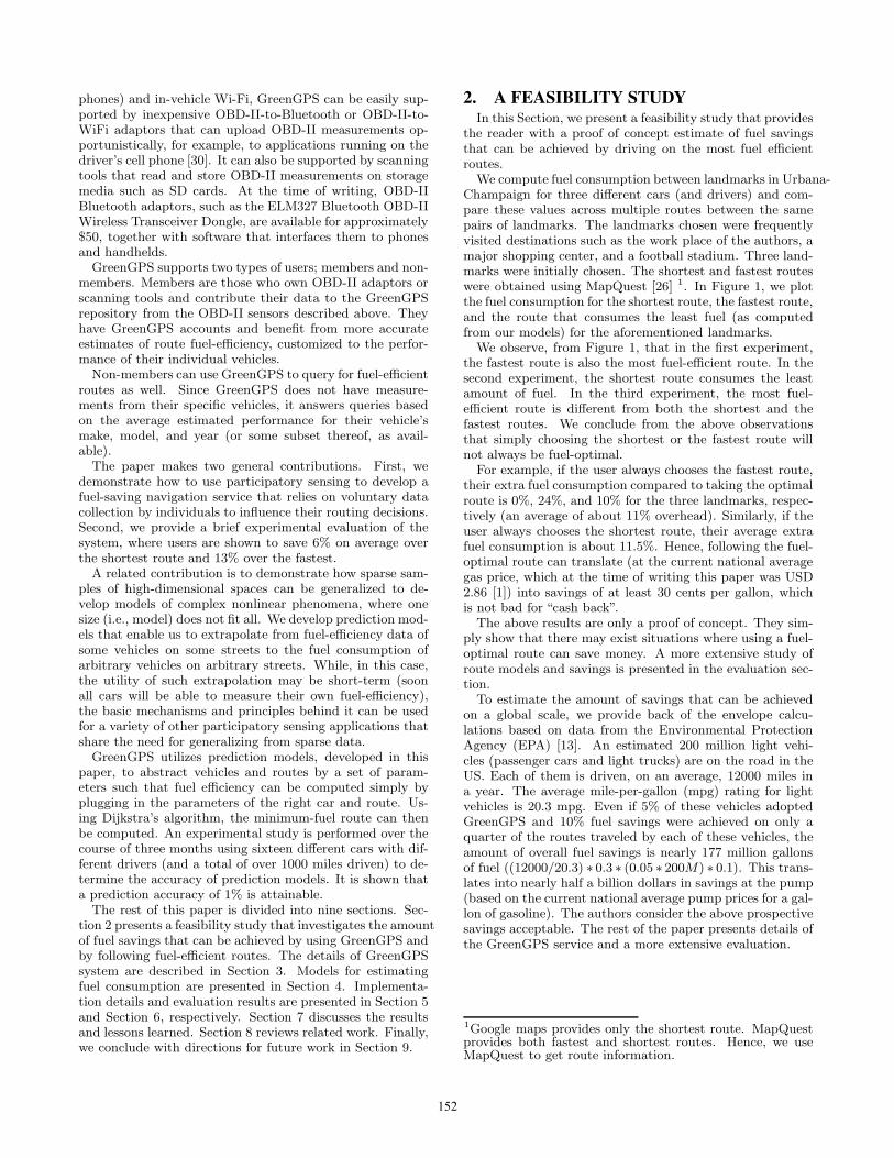
lar map application, such as Google maps [19] or MapQuest[26]. Google maps and MapQuest provide the shortest orfastest routes between two points, whereas GreenGPS com-putes the most fuel-efficient route. A snapshot of the Web-based GreenGPS’s user interface is shown in Figure 2 alongwith the most fuel efficient route between two points for auser with a Toyota Celica, 2001. In the following subsec-tions, we will discuss the GreenGPS concept, then presentthe participatory sensing framework that we utilize for datacollection and data sharing and the specifics of the hardwareused for the purpose of data collection.

3.1 The GreenGPS ConceptIndividuals who want to compute the most fuel-efficient

route between two points enter the source and destinationaddress via the interface provided by GreenGPS. Membersof GreenGPS (i.e., those individuals who contributed partic-ipatory data) can register their vehicles that were used fordata collection. Hence, GreenGPS can compute the routespecifically for the registered vehicle. Other users may en-ter their vehicle’s make, model, and year of manufacture.Since different vehicles have different fuel consumption char-acteristics, these car details are used to compute the mostfuel-efficient route for the given vehicle brand. The advan-tage for the users who contribute data is that the systemprovides better estimates of the most fuel-efficient routes tothese individuals, thus allowing them to have higher savings.

Currently, it is impractical to assume that GreenGPS mem-bers will measure all city streets and cover all vehicle types.Instead, measurements of GreenGPS members are used tocalibrate generalized fuel-efficiency prediction models. Thesemodels, discussed in Section 4, show that the fuel consump-tion on an arbitrary street can be predicted accurately fromset of static street parameters (e.g., the number of trafficlights and the number of stop signs) and a set of dynamicstreet parameters (such as the average speed on the streetor the average congestion level), plus of course the vehicleparameters (e.g., weight and frontal area). It is the mathe-matical model describing the relation between these generalparameters and fuel-efficiency that gets estimated from par-ticipant data. Hence, the larger and more diverse is the setof participants, the better the generalized model.

0

0.05

0.1

0.15

0.2

0.25

1 2 3

Fue

l con

sum

ed (

gallo

ns)

Experiment number

Shortest routeFastest route

Fuel-efficient route

Figure 1: Figure showing fuel consumption for mul-tiple routes between multiple selected landmarks fordifferent cars and drivers

Figure 2: Figure showing the user interface ofGreenGPS with the most fuel efficient route be-tween two points on the map for a Toyota Celica,2001.

For most streets, static street parameters can be readilyobtained from traffic databases. For example, the numberof traffic lights and the number of stop signs on streets canbe obtained from the red light database [20]. Dynamicallychanging parameters such as the congestion levels or averagespeed are more tricky to obtain. In larger cities, real-timetraffic monitoring services can supply these parameters [35].Many GPS device vendors, such as TomTom, also collectand provide congestion information. Finally, participatorysensing applications, such as Traffic Analyzer [17] and Car-Tel [24], have been described in prior literature that havethe potential to provide congestion and speed data.

In this paper, speed information is obtained from the col-lected data using the hardware described in the next sec-tion. The speed data is aggregated for different city blocks,based on the GPS data. Thus, given a street name (or thelatitude/longitude of a location), GreenGPS provides theaverage speed information for the corresponding block.

3.2 A Participatory Sensing FrameworkWe utilize a participatory sensing framework developed in

our prior work, called PoolView [17], to implement GreenGPS.PoolView facilitates developing data collection applications.It provides a client-side interface for data upload and deliv-ers all data to a central server called the aggregation server ,that is application-specific. We implemented GreenGPS bywriting our aggregation server for PoolView. An individ-ual who wants to share their OBD-II sensor data can thusdownload the client side software of PoolView, and use it toupload their data to the GreenGPS aggregation server. Theaggregation server uses these data to calibrate models thatrelate street and vehicle parameters to fuel-efficiency andoffers the GreenGPS query interface for fuel-efficient routes.

Individuals who wish to contribute OBD-II data to GreenGPSinstall, in their vehicle, a commercial OBD-II scanner alongwith a GPS unit. In our deployment, we use one such off-the-shelf device for data collection purposes, called Dash-Dyno [4], shown in Figure 3. The DashDyno’s OBD-II scan-ner is interfaced to a Garmin eTrex Legend GPS [18] to getlocation data. The DashDyno records trip data (including

153

Garmin’s GPS location) on an SD card that the user lateruploads it to the GreenGPS server.

Figure 3: Hardware used for data collection

A total of 16 parameters are obtained from the car and theGPS, the most important of them being instantaneous vehi-cle speed, total fuel consumption, rate of fuel consumption,latitude, longitude, and time.

4. GENERALIZING FROM SPARSE DATAIn this section, we demonstrate the foundations of one

of the key mechanisms in participatory sensing applicationsthat are tolerant to conditions of sparse deployment; namely,the generalization from sparse multidimensional data. Suchgeneralization is complicated by the fact that, in high-dimensionaldata sets, one size does not fit all. Hence, for example, devel-oping a single regression model to represent all data is highlysuboptimal. In the case of GreenGPS, the lack of widespreadavailability of OBD-II scanner tools suggests that the datacontributed by users of our participatory sensing applicationwill be a sparse sampling of routes and cars. Hence, we aimto use data collected by a smaller population to build modelscapable of predicting the fuel consumption characteristics ofa larger population. Admittedly, the conditions of sparsedeployment are typically temporary, making the above con-tribution short-lived in nature. Nevertheless, it solves a keyproblem at a critical phase of most newly deployed systems,which makes it important. Before we explain the detailsof the generalization mechanism, we will provide a brief de-scription of our data collection for the purpose of developingmodels.

4.1 Data CollectionThe vision for GreenGPS, when fully deployed, is to col-

lect data from everyday users, which can be employed toupdate and refine predictions of fuel consumption when suchusers (or others with similar vehicles) embark on new itineraries.Having said so, for the purposes of this paper, we con-ducted a limited proof-of-concept study involving sixteenusers (with different cars) over the course of three months.A total of over 1000 miles were driven by our users to con-struct the initial models. Figure 4 shows a partial map ofthe paths on which data were collected. The details of thecar make, model, year, and the number of miles of datacollected for each car are summarized in Table 1.

In the aforementioned experiments, each user was asked todrive among a specific set of landmarks in the city. We split

Figure 4: Coverage map for the paths on which datawere collected

Car make Car model Car year Miles drivenFord Taurus 2001 135

Toyota Solara 2001 45BMW 325i 2006 70Toyota Prius 2004 140Ford Taurus 2001 136Ford Focus 2009 95

Toyota Corolla 2009 45Honda Accord 2003 102Ford Contour 1999 22

Honda Accord 2001 18Pontiac Grand Prix 1997 25Honda Civic 2002 11

Chevrolet Prizm 1998 16Ford Taurus 2001 10

Mazda 626 2001 9Toyota Celica 2001 120

Hyundai Santa Fe 2008 22

Table 1: Table summarizing the cars used and theamount of data collected

each drive into smaller segments to capture the variation inthe fuel consumption on individual streets. These segmentswere the “samples” used to capture the variables affectingfuel consumption and develop initial prediction models.

4.2 Derivation of Model StructureThe first part of data generalization is to derive a model

structure. The structure describes how various parametersare related, but does not evaluate the various constants andproportionality coefficients. In this case, we derive the struc-ture of fuel prediction models from physical analysis. Theanalysis is straightforward but is included for completeness.

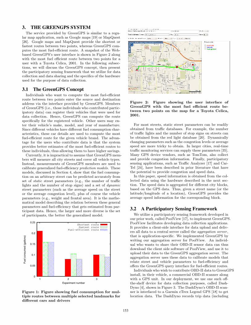
To motivate the need for modeling, we plot the distribu-tion of miles per gallon (mpg) for all the data collected inFigure 5. We observe from this figure that the distribution isnearly uniform with the mpg values varying between 5 and50. The standard deviation of the mpg distribution is 9.12mpg, which is pretty high. Hence, an appropriate modelis needed to estimate the fuel consumption on various seg-ments.

154

10 20 30 40 500

0.01

0.02

0.03

0.04

0.05

0.06

0.07

MPG

MP

G D

istr

ibut

ion

Figure 5: Figure showing the real mpg distributionfor all the sixteen users

The inputs to our prediction model include segment pa-rameters and car parameters. We do not consider driverfactors in the model because the sample size of drivers wassmall in our dataset. We will explore the effect of driverfactors on fuel consumption in our future work. Note that,we are interested in predicting long-term fuel consumptiononly. While actual savings of a user on individual commutesto work may vary, the user might be more concerned withtheir net long-term savings. Hence, it is important to cap-ture only the statistical averages of fuel consumption. Aslong as the errors have near zero mean, the savings are ac-curate in the long term. As a given user drives more seg-ments, a value of interest is the total end-to-end predictionerror that results (which improves over time as the individ-ual positive and negative segment errors cancel out). Wecall that end-to-end error the cumulative error . It is usefulto normalize that error to the total distance driven. We callthe result cumulative percentage error . It represents how farwe are off in our estimate of total fuel consumption.

We derive the model structure for fuel consumption fromthe basic principles of physics. Many such models exist inprior literature [7, 15, 36], which simplifies the task. Wedivide the parameters that affect fuel consumption into (i)static segment parameters, namely, numbers of stop signs(ST ), numbers of traffic lights (TL), distance traveled (Δd)and slope (θ), (ii) dynamic segment parameters, namely, av-erage speed (v̄), and car specific parameters, namely, weightof the car (m) and car frontal area (A).

The approximated fuel consumption model as a functionof the above parameters was derived and can be found in theAppendix. It is given as follows (where gpm is the inverseof mpg and the unit of measure is gallons per mile):

gpm = k1mv̄2 (ST + νTL)

Δd+ k2m

v̄2

Δd

+ k3mcos(θ) + k4Av̄2 + k5msin(θ) (1)

We plot the distributions for various parameters (for indi-vidual segments) in Equation 1 for the data that we collectedin Figure 6. In the next section, we show that the coefficientsof our model, k1, k2, k3, k4 and k5 differ among different ve-hicles making it harder to generalize from vehicles we havedata for to those we do not.

4.3 Model Evaluation: One Size Fits All?Regression analysis is a standard technique for estimating

coefficients of models with known structure. In this section,

we demonstrate that a single regression model is a bad fitfor our data. Said differently, while a regression model thataccurately predicts fuel consumption can be found for eachcar from data of that one car, the model found from thecollective data pool of all cars is not a good predictor forany single vehicle. Hence, in a sparse data set (where datais not available for all cars); it is not trivial to generalize. Weillustrate that challenge by first evaluating the performanceof car models obtained from their own data (which is good),then comparing it to the trivial generalization approach: onethat finds a single model based on all car data then uses itto predict fuel consumption of other cars. A solution to thechallenge is presented in the next section.

One should add that while the generalization challengeis common to many participatory sensing applications, ourevaluation is not intended to be a definitive study on vehic-ular fuel consumption. For example, we evaluate fuel con-sumption in Urbana-Champaign only, which is quite flat.Hence, θ = 0 is a good approximation. (We therefore setthe last term, k5msin(θ), of our physical model to zero, sok5 is no longer needed.) Furthermore, the city is rarely con-gested. Moreover, the range of cars used in the study israther skewed towards sedans, and hence not representativeof the diversity of cars on the streets. Fortunately, eventhis rather homogeneous data set is sufficient to show thatgeneralization is hard.

First, we determine the length of the segment empirically.We vary the segment length from 0.5 miles to 2 miles in in-crements of 0.5 miles and evaluate the accuracy of our modelin each of these cases. We observed that the accuracy of themodel is best when the segment length is 1 mile. Hence, wefix the segment length to be 1 mile in the rest of our exper-iments. We evaluate the accuracy of models derived fromvehicle data using a cross validation approach. We choose arandom data point (i.e., a given segment of a street drivenby some car) to predict fuel consumption for. We then useother points to train a model. We distinguish models basedon other segments of the same car from models based ondata from other cars in predicting the fuel consumption ofthe one segment. The 4th and 5th columns of Table 2 sum-marize the resulting errors, respectively, for a fraction of theused cars.

Car Car Car Individual Generalmake model year cumulative cumulative

error % error %(magnitude) (magnitude)

Hyundai Santa Fe 2008 2.89 23.63Honda Accord 2003 0.89 15.3Ford Contour 1999 0.83 91.4Ford Focus 2009 0.12 27.35Ford Taurus 2001 0.75 24.85

Toyota Corolla 2009 0.61 89.97Ford Taurus 2001 0.56 6.9

Table 2: Table summarizing the cumulative percent-age errors for the individual car models and the gen-eralized case when all the data (except one car) isused to obtain the model

We also plot the error distribution for individual segments(for one car) in Figure 7. We observe that this distribution is

155

−1 0 1 2 3 4 5 60

0.05

0.1

0.15

0.2

0.25

0.3

0.35

0.4

Number of traffic lights

Tra

ffic

light

dis

trib

utio

n

(a) Traffic light distribution

−1 0 1 2 3 4 5 60

0.1

0.2

0.3

0.4

0.5

0.6

0.7

0.8

Number of stop signs

Sto

p si

gn d

istr

ibut

ion

(b) Stop sign distribution

0 20 40 60 800

0.05

0.1

0.15

0.2

Speed (mph)

Spe

ed d

istr

ibut

ion

(c) Average speed distribution

Figure 6: Figures showing the distributions of number of traffic lights, stop signs, and average speed

near normal and the mean is near zero (0.26%). We observea similar distribution for other cars too.

−20 −10 0 10 200

0.02

0.04

0.06

0.08

0.1

Percentage segment errors

Seg

men

t err

or d

istr

ibut

ion

Figure 7: Figure showing the segment error distri-bution for one car

We also observe from the Table 2 that the cumulative per-centage error for individual car models are quite good. Mostof them are below 2%. On the other hand, when we predictone car’s consumption using data from other cars, the errorsare quite high. This suggests the existence of non-trivial biasin error that does not cancel out by aggregation. In the nextsection, we propose a way to mitigate this problem based ongrouping cars into clusters, such that prediction can be donebased on other similar cars by some metric of similarity.

4.4 Model ClusteringThe above suggests a need for better generalization over

vehicle data. Different car types behave differently. Eventhough the model is parameterized by factors such as carweight and frontal area, they are not enough to account fordifferences among cars. This is a common problem in high-dimensional data sets collected in participatory sensing ap-plications. The question becomes, if we cannot generalizeover the whole set, can we generalize over a subset of di-mensions?

A solution is borrowed from the general literature on datacubes [21]. Data cubes are structures for Online Analyt-ical Processing (OLAP) that are widely used for multidi-mensional data analysis. They group data using multipleattributes and extract similarities within each group. Forexample, previous work showed how to efficiently construct

regression models for various subsets of data [10]. The datacube framework can thus help compute the optimal gener-alization hierarchy in that it can help generalize data basedon those dimensions that results in the minimum modelingerror.

We consider three major attributes (data dimensions) ofa given car: make, year, and class. Based on these threeattributes, data can be grouped in eight ways. At one ex-treme, all cars may be grouped together, thus producing asingle regression model (which we have shown is not accept-able). At the other extreme, cars can be partitioned intoclusters based on their (make, year, class) tuple. A separatemodel is derived for each cluster. Therefore, a 2001 com-pact Ford is modeled differently from a 2001 mid-size Ford,a 2002 compact Ford or a 2001 compact Toyota.

0

1

2

3

4

5

6

Clustering

AllM

akeYear

Make/Year

Class

Make/Class

Year/Class

Ave

rage

cum

ulat

ive

erro

r pe

rcen

tage

Figure 8: Cumulative error percentage of the modelsobtained from various clustering approaches

Between these two extremes, to find out which clusteringscheme gives the best accuracy, we obtain the cumulativepercentage error for each scheme. The results, summarizedin Figure 8, show that different generalizations have differ-ent quality. These generalizations are somewhat better thanusing all car data lumped together. While our data set istoo small to make general conclusions (from only 16 cars),as more data are collected in a deployed participatory sens-ing application (e.g., say deployment reaches 100s of cars),progressively better generalizations can be attained.

To use results of Figure 8, one would build models for eachpair of make and year (the lowest error clustering scheme).If a car is encountered for which we do not have data on

156

its (make, year) cluster, we go one level up and use (make)clusters or (year) clusters as generalizations for the (make,year) cluster. If there are no models corresponding to eithermake or year of a given car, we have no recourse but togo one level up and use the model computed from all data.Figure 9 depicts the generalization process among variousmodel clusters.

Make Year

All

Make, Year

Figure 9: Model generalization from fine grainedclusters

Car Car Car Cumulativemake model year error %

Hyundai Santa Fe 2008 0.73Honda Accord 2003 1.01Ford Contour 1999 1.42Ford Focus 2009 2.7Ford Taurus 2001 3.38

Toyota Corolla 2009 1.28

Table 3: Table showing the cumulative error per-centage for each individual car when model cluster-ing is used

We evaluate the performance of our model clustering tech-nique by measuring how accurately an individual car can bemodeled using the data from cars with similar make or year.Specifically, we construct the model cluster while removingdata of a certain car type. We use the model cluster to es-timate the fuel consumption for a given car. The resultingcumulative error percentage is presented in Table 3.

To put the above results in perspective, the reader is re-minded that the nature of the landscape in Urbana-Champaignlimits our study in that we do not have data on hilly terrain.The study would have been more interesting if conducted onuneven grounds, where changes in incline modulate fuel con-sumption. We expect that future data collected will be usedto evolve our current model by considering the terrain (θ inEquation 1) parameter. Further, new data collected will beused to update the model. Another limitation of our model-ing approach arises from the class of cars for which data hasbeen collected. We observe from Table 1 that the majorityof the cars are sedans (with the exception of one SUV). Weobserve that the generalization tree (Figure 9) does not usethe class of the car. This generalization tree is specific to

the dataset collected. The point of this section is to illus-trate an approach to improve prediction in the temporarybut important conditions of sparse deployment. Ultimately,when all cars have their own OBD-II readers supplying datato drivers’ cell-phones, we shall not need the generalizationscheme described above.

5. IMPLEMENTING GREENGPSThe GreenGPS server combines several open source soft-

ware services to provide the fuel-efficient route computationservice. The various modules that are part of the GreenGPSimplementation are depicted in Figure 10. GreenGPS main-tains the map of a given area as an OpenStreetMap (OSM) [29].OSM is the equivalent of Wikipedia for maps, where data arecollected from various free sources (such as the US TIGERdatabase [37], Landsat 7 [27], and user contributed GPSdata) and an editable street map of the given area is createdin an XML format. The OSM map is essentially a directedgraph, which is composed of three basic object types, nodes,ways, and relations. A node has fixed coordinates and ex-presses points of interest (e.g. junction of roads, Marriotthotel). A way is an ordered list of nodes with tags to spec-ify the meaning of the way, e.g. a road, a river, a park.A relation models the relationship between objects, whereeach member of the relation has a specific role. Relationsare used in specifying routes (e.g. bus routes, cycle routes),enforcing traffic (e.g. one way routes).

GreenGPS maintains the street variables affecting fuelconsumption as additional parameters in the OSM map.This information is stored as a tag/value pair in the wayobject, where tag is a street parameter and value is the corre-sponding value of the parameter. We are currently workingon populating the street variables into the OSM databasefor Urbana-Champaign in an automated manner. Further,the car and driver specific parameters are maintained in aseparate database. The model to compute fuel consumptionon a given way (for a given car and driver) queries thesedatabases and computes the fuel consumption on the way.

The OBD-II data shared by individuals is used to com-pute regression models that predict the fuel consumptionon specific streets given the car details (e.g. make, model,age) and driver behavior. The regression variables which arestreet specific are stored in the OSM map database, whereasthe car and driver specific variables are stored in a similardatabase.

5.1 Model Clustering ImplementationGreenGPS implements the model clustering technique de-

scribed in Section 4.4 using Data Cubes [21].We implement a 3-dimensional (make, class, year) regres-

sion cube [10] in C++. Each one mile segment is organizedas a row in a database where five of its attributes are thevalues of physical model parameters (see Section 4.2) andare used for regression. Three other attributes (make, class,year) are used for grouping. After computing the regres-sion models for all clusters (i.e. materializing the cube),search for a specific triple of (make, class, year) is done con-secutively within the (make, year) cluster, the (make) clus-ter, and the (year) cluster. The first regression model thatmatches the query is used for prediction.

5.2 Routing in GreenGPSRouting is achieved in GreenGPS by customizing the open

source routing software, Gosmore [28]. Gosmore is a C++

157

routes

Querymapdatabase

Update mapdatabase

Users contributetheir OBD−II data

databasecar/driver Query

Update car/driver database

GUI frontend

Start and

Fuel−optimal route and estimated fuel consumedDisplay routes

User input

destination address

Convert street

Geocoder

addresses tolatitude/longitude latitude/longitude

Start, destination

GosmoreRouting to findfuel−optimal,

shortest and fastest

GreenGPS Server

Map OBD−II fuel

OBD−II Mapper

data to OSM data

Maintain map dataOSM Database

street parametersin XML format parameters

driver specificMaintain car and

Car/DriverDatabase

Figure 10: Figure depicting the various modules of GreenGPS

based implementation of a generic routing algorithm thatprovides shortest and fastest routes between two arbitraryend-points. Gosmore uses OSM XML map data for doingrouting. Gosmore’s routing algorithm is a heuristic that bydefault computes the shortest route. This routing algorithmcan be thought of as a weighted Dijkstra’s algorithm on theOSM map, where the nodes of the graph are OSM nodes andthe edges of the graph are OSM ways and the weights of theedges are the lengths (distance) of the ways. The fastestroute is computed by multiplying the distance by an inversespeed factor (thus giving lower weights to faster ways). Ourfuel-optimal routing algorithm multiplies the distance by aninverse mpg (miles per gallon) metric that results in lowerweights for fuel-optimal ways.

5.3 Other Implementation IssuesStreet address inputs provided by the user are translated

into latitude/longitude pairs using the open source geocod-ing perl module, Geo::Coder::US. This module is used forgeocoding US addresses only. Geocoding is the process offinding corresponding latitude/longitude data given a streetaddress, intersection, or zipcode.

The GUI frontend to display the fuel-optimal route (shownin Figure 2) utilizes Microsoft Bing maps. Routes are colorcoded and rendered as polylines on Bing maps. For example,the fuel-optimal route is a “green” color polyline.

When a query is posed to GreenGPS for the fuel-optimalroute between the start address and destination address, theaddresses are first geocoded into their corresponding latitudeand longitude pairs using the geocoder module. The latitudeand longitude pairs of the start and destination addressesare then fed to the routing module which computes the fuel-optimal route (along with the shortest and fastest routes)using the OSM XML database and the prediction modelsof fuel consumption on streets (computed from the OBD-IIsensor data contributed by users). The computed routes arethen displayed on the Bing maps based GUI frontend.

6. EVALUATIONWe evaluate the performance of GreenGPS in two stages.

First, we evaluate the performance of our model by using itto predict the end-to-end fuel consumption for long routes.Second, we evaluate the potential fuel savings of an individ-ual using GreenGPS.

6.1 Model AccuracyWe first evaluate the accuracy of our prediction model in

estimating fuel consumption on long routes. These routesare continuous sequences of segments that individuals drove.Only six cars are used in this experiment2 because the data

2Ford Focus, 2009; Ford Taurus 2001; Toyota Corolla, 2009;

158

from the rest of the cars did not include multiple paths (andhence we would not be able to do path-based cross valida-tion, where data collected on one path is used to predictfuel consumption on another). We consider the path erroras the end-to-end prediction error for the given path (whichis the metric used for evaluation in Section 4). For cross val-idation, we remove the data points associated with a givenpath and obtain a model for the car, then obtain the errorin predicting fuel consumption for this path based on thecomputed model. We repeat the above for all the paths.

The entire path error distribution corresponding to theabove experiment when prediction for each car is used basedon data of the same car (on other paths) is shown in Fig-ure 11. We observe that the path error distribution is nearlynormal and that the mean of this distribution is near zero(<1%). We conduct a similar experiment to derive the patherror distribution that is achieved by employing clusteringsuch that fuel consumption of cars is predicted from that ofother cars in the nearest cluster. To experiment with predic-tion accuracy of clusters, we remove the data points for eachcar (as if that car was not known to the system) and clusterthe rest of data points, as described in Section 4.4, based onmake, year, and both. Fuel consumption of the removed caris then predicted using the nearest cluster. Namely, we firstcheck if a cluster exists with the same car make and year.If no such cluster exists, we check for a cluster of the samemake or the same year, respectively. Finally, a model basedon all car data is used if all the previous steps fail. Theprediction error for each path is computed as before and thedistribution is presented in Figure 12. Again, a normal dis-tribution of the path errors is observed with near zero mean(<4%).

−20 −10 0 10 200

0.02

0.04

0.06

0.08

0.1

0.12

0.14

0.16

0.18

Path error percentage

Pat

h er

ror

perc

enta

ge d

istr

ibut

ion

Figure 11: Distribution of path error percentageswhen training is done using individual cars

In order to understand how path errors vary with pathlengths, we bin the paths based on their length and computethe average of the absolute path errors as a function of pathlength. We repeat this experiment for the case where modelsare derived for each car individually and the case where mod-els are derived for clusters and the nearest cluster is used.We plot the mean of the absolute path errors for varyingpath lengths in Figure 13. We observe from Figure 13 thatthe error decreases with increasing path length for both theindividual and cluster based models. As expected, models

Ford Taurus, 2001, Honda Accord, 2001; and Ford Taurus,2001.

−20 −10 0 10 200

0.05

0.1

0.15

0.2

0.25

0.3

0.35

Path error percentage

Pat

h er

ror

perc

enta

ge d

istr

ibut

ion

Figure 12: Distribution of path error percentagesfor the clustering approach

0 5 10 15 200

5

10

15

20

25

30

35

Path length (miles)

Pat

h pe

rcen

tage

err

or

ClusteringIndividual

Figure 13: Mean path error when path length isvaried for individual car models and cluster basedmodels

based on the owner’s car do better than models based onthe nearest cluster, but the cumulative error continues todecrease with distance driven, which is what we want. Wehave not explored if this holds true when the commutes havelarge dynamics in speeds, such as in larger cities. The cur-rent data set is limited in that it was collected in a fairlyquiet town.

From the perspective of building participatory sensingapplications, the above suggests the importance of findingmodels that do not have biased error . Since the models of-ten try to predict aggregate or long-term behavior (such aslong term exposure to pollutants, annual cost of energy con-sumption, eventual weight-loss on a given diet, etc), if theerror in day-by-day predictions is normally distributed withzero mean, the long-term estimates will remain accurate.Hence, rather than worrying about exact models, GreenGPSattempts to find unbiased models, which is easier.

159

6.2 Fuel SavingsIn this section, we evaluate the fuel savings achieved when

using the GreenGPS system. As we outlined in the imple-mentation section, we are integrating the street parameterssuch as the stop signs, traffic lights, and average speed infor-mation into the OSM database. To evaluate fuel savings, wechose landmarks in the city of Urbana-Champaign that theauthors visit in their daily commutes, such as work, gym,frequently visited restaurants, and shopping complexes. Toeliminate subjective choice of routes between the selectedlandmarks, each of the authors selected a pair of landmarksthen looked up both the shortest route and fastest routebetween these landmarks on MapQuest. The person thendrove eight round trips (of approximately 20-40 minuteseach) between their selected pair of landmarks; four on theshortest route and four on the fastest route, recording ac-tual fuel consumption for each round trip. The landmarkstogether with the shortest and fastest routes are shown inFigure 14. We then used the GreenGPS system to predictwhich of the two compared routes for each pair of landmarksis the better route, which it did correctly in every case.

The fuel consumption data for each roundtrip on the short-est and fastest routes for all the cars in this experiment areshown in Table 4.

We observe from Table 4 that the fuel-optimal route fordestinations of the Honda Accord and Ford Taurus was theshortest route, whereas, for the other three destinations itwas the fastest route. Hence, picking the shortest or fastestroutes consistently is not optimal. To confirm that the dif-ferences in fuel consumption between the compared routesare not due to measurement noise, we tested the statisticalsignificance of the difference in means using the two pairedt-test. The test yielded that the differences are statisticallysignificant with a confidence level of at least 90%. The av-erage savings (by choosing the correct route over the alter-native) for each pair of landmarks and car are summarizedin Table 4.

Comparing the total fuel consumed on the optimal routeto the average of that consumed on the shortest route andfastest route (assuming the driver guesses at random in theabsence of GreenGPS), the savings achieved are roughly 6%over the shortest path and 13% over the fastest, which isconsistent with data we reported earlier in the feasibilitystudy.3. This is by no means statistically significant, sinceonly a handful of routes were used in the experiments above,but it nevertheless shows promise as a proof of concept.

7. LESSONS LEARNEDThis section presents, in its two respective subsections,

a brief discussion of our experiences with the GreenGPSservice and the limitations of the current study.

7.1 Experiences with GreenGPSSeveral lessons were learned from GreenGPS, as an exam-

ple of participatory sensing applications. First, we observedthat data cleaning is an important problem and it is appli-cation dependent. We had several occasions when severalfields were missing from the data. For example, the GPSsometimes failed to communicate with the DashDyno andthe location fields were then empty. A simple scheme was

3The feasibility study used different routes from those re-ported above

used to filter complete datasets from those that were missingvalues. Another data-related issue was the presence of noisein the data. For example, in our setup, we observed that (insome car models) whenever the GPS communicated withthe DashDyno, the fuel rate measurement had a large spike.This was likely due to improper use of sensor IDs, which ledto data overwriting. Solutions have to be developed thatfilter the noise at the source. For example, we developed asimple filter (as a plugin to PoolView) that removes outliersfrom the data before storing it. An application-specific chal-lenge was observed due to the slight variations in the OBD-IIstandards among different cars. For example, we observedthat the Toyota Prius (by default) outputs the speed and fuelmeasurements in the metric system, rather than the Imperialsystem (which happens to be the default for the remainingcars in our dataset). It is harder to propose generic solu-tions to such problems. They suggest, however, that unlikesmall embedded systems, participatory sensing applicationsinvolve a much larger number of heterogeneous components(e.g., different car types in GreenGPS). As such componentsinteract with each other or with aggregation services, subtlecompatibility problems will play an increasing role. Trou-bleshooting techniques are needed that are good at identify-ing problems resulting from unexpected or bad interactionsamong different individually well-behaved components. Thisis to be contrasted, for example, with debugging tools thatattempt to find bugs in individual components.

Next, privacy challenges come to the forefront in par-ticipatory sensing systems. A large class of participatorysensing systems monitor location information continuously,which poses significant privacy issues. Simple anonymiza-tion of data will not work in such situations, as the GPStraces can lead to privacy breaches (e.g., reveal the homelocation of the user and thus uncover their identity). Tech-niques such as the ones proposed in [17] and [31], which relyon data perturbation can be used to preserve privacy, whilestill allowing accurate modeling. In our current study, indi-vidual users simply switch off data collection devices whenthey feel the need for privacy.

Finally, another lesson learned relates to the initial ex-perimental deployment of participatory sensing systems. Amajor hurdle in getting participatory sensing systems off theground is to provide the right incentives to the individuals(who are part of the system) [32]. We believe that the initialdeployment, which tends to be sparse, should be carefullydesigned in order to provide incentives for larger adoption.It should therefore be useful from the very early stages.

7.2 Limitations of Current StudyApart from the limitations arising from the small size of

the data set, discussed earlier, we also make the follow-ing observations. As expected, the main factors affectingfuel consumption of a vehicle on a path are the averagespeed, the speed variability (estimated by averaging thespeed squared), and the engine idle time (estimated fromthe number of stop signs and stop lights on the path). Alimitation of the study is that we did not explore the use ofreal-time traffic conditions for purposes of fuel estimation.Rather, we opted to use statistical averages of speed, speedvariability and idle time. It is easy to see how such sta-tistical averages can be computed for different hours of theday and different days of the week given a sufficient amountof historical data, yielding expected fuel consumption (in

160

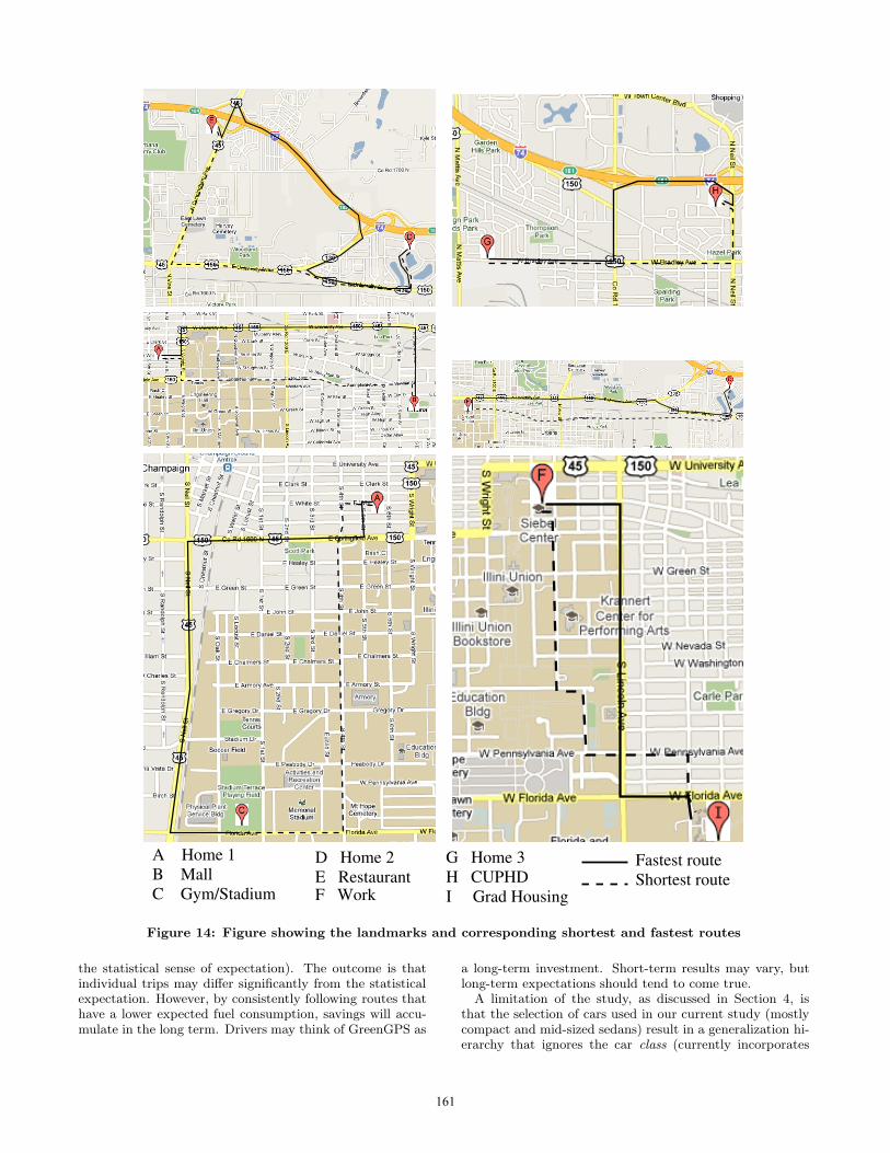
A Home 1B MallC Gym/Stadium

D Home 2E Restaurant F Work

G Home 3

I Grad HousingH CUPHD

Fastest routeShortest route

Figure 14: Figure showing the landmarks and corresponding shortest and fastest routes

the statistical sense of expectation). The outcome is thatindividual trips may differ significantly from the statisticalexpectation. However, by consistently following routes thathave a lower expected fuel consumption, savings will accu-mulate in the long term. Drivers may think of GreenGPS as

a long-term investment. Short-term results may vary, butlong-term expectations should tend to come true.

A limitation of the study, as discussed in Section 4, isthat the selection of cars used in our current study (mostlycompact and mid-sized sedans) result in a generalization hi-erarchy that ignores the car class (currently incorporates

161

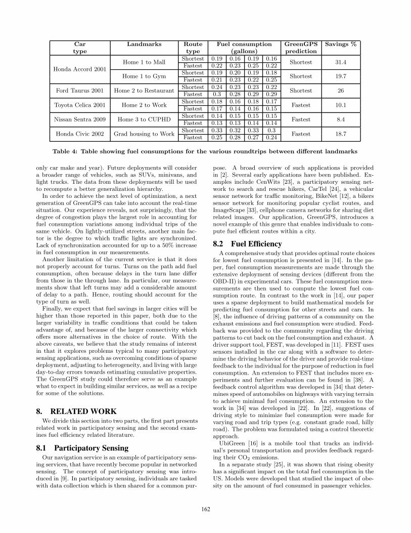
Car Landmarks Route Fuel consumption GreenGPS Savings %type type (gallons) prediction

Honda Accord 2001Home 1 to Mall

Shortest 0.19 0.16 0.19 0.16Shortest 31.4

Fastest 0.22 0.23 0.25 0.22

Home 1 to GymShortest 0.19 0.20 0.19 0.18

Shortest 19.7Fastest 0.21 0.23 0.22 0.25

Ford Taurus 2001 Home 2 to RestaurantShortest 0.24 0.23 0.23 0.22

Shortest 26Fastest 0.3 0.28 0.29 0.29

Toyota Celica 2001 Home 2 to WorkShortest 0.18 0.16 0.18 0.17

Fastest 10.1Fastest 0.17 0.14 0.16 0.15

Nissan Sentra 2009 Home 3 to CUPHDShortest 0.14 0.15 0.15 0.15

Fastest 8.4Fastest 0.13 0.13 0.14 0.14

Honda Civic 2002 Grad housing to WorkShortest 0.33 0.32 0.33 0.3

Fastest 18.7Fastest 0.25 0.28 0.27 0.24

Table 4: Table showing fuel consumptions for the various roundtrips between different landmarks

only car make and year). Future deployments will considera broader range of vehicles, such as SUVs, minivans, andlight trucks. The data from these deployments will be usedto recompute a better generalization hierarchy.

In order to achieve the next level of optimization, a nextgeneration of GreenGPS can take into account the real-timesituation. Our experience reveals, not surprisingly, that thedegree of congestion plays the largest role in accounting forfuel consumption variations among individual trips of thesame vehicle. On lightly-utilized streets, another main fac-tor is the degree to which traffic lights are synchronized.Lack of synchronization accounted for up to a 50% increasein fuel consumption in our measurements.

Another limitation of the current service is that it doesnot properly account for turns. Turns on the path add fuelconsumption, often because delays in the turn lane differfrom those in the through lane. In particular, our measure-ments show that left turns may add a considerable amountof delay to a path. Hence, routing should account for thetype of turn as well.

Finally, we expect that fuel savings in larger cities will behigher than those reported in this paper, both due to thelarger variability in traffic conditions that could be takenadvantage of, and because of the larger connectivity whichoffers more alternatives in the choice of route. With theabove caveats, we believe that the study remains of interestin that it explores problems typical to many participatorysensing applications, such as overcoming conditions of sparsedeployment, adjusting to heterogeneity, and living with largeday-to-day errors towards estimating cumulative properties.The GreenGPS study could therefore serve as an examplewhat to expect in building similar services, as well as a recipefor some of the solutions.

8. RELATED WORKWe divide this section into two parts, the first part presents

related work in participatory sensing and the second exam-ines fuel efficiency related literature.

8.1 Participatory SensingOur navigation service is an example of participatory sens-

ing services, that have recently become popular in networkedsensing. The concept of participatory sensing was intro-duced in [9]. In participatory sensing, individuals are taskedwith data collection which is then shared for a common pur-

pose. A broad overview of such applications is providedin [2]. Several early applications have been published. Ex-amples include CenWits [23], a participatory sensing net-work to search and rescue hikers, CarTel [24], a vehicularsensor network for traffic monitoring, BikeNet [12], a bikerssensor network for monitoring popular cyclist routes, andImageScape [33], cellphone camera networks for sharing dietrelated images. Our application, GreenGPS, introduces anovel example of this genre that enables individuals to com-pute fuel efficient routes within a city.

8.2 Fuel EfficiencyA comprehensive study that provides optimal route choices

for lowest fuel consumption is presented in [14]. In the pa-per, fuel consumption measurements are made through theextensive deployment of sensing devices (different from theOBD-II) in experimental cars. These fuel consumption mea-surements are then used to compute the lowest fuel con-sumption route. In contrast to the work in [14], our paperuses a sparse deployment to build mathematical models forpredicting fuel consumption for other streets and cars. In[8], the influence of driving patterns of a community on theexhaust emissions and fuel consumption were studied. Feed-back was provided to the community regarding the drivingpatterns to cut back on the fuel consumption and exhaust. Adriver support tool, FEST, was developed in [11]. FEST usessensors installed in the car along with a software to deter-mine the driving behavior of the driver and provide real-timefeedback to the individual for the purpose of reduction in fuelconsumption. An extension to FEST that includes more ex-periments and further evaluation can be found in [38]. Afeedback control algorithm was developed in [34] that deter-mines speed of automobiles on highways with varying terrainto achieve minimal fuel consumption. An extension to thework in [34] was developed in [22]. In [22], suggestions ofdriving style to minimize fuel consumption were made forvarying road and trip types (e.g. constant grade road, hillyroad). The problem was formulated using a control theoreticapproach.

UbiGreen [16] is a mobile tool that tracks an individ-ual’s personal transportation and provides feedback regard-ing their CO2 emissions.

In a separate study [25], it was shown that rising obesityhas a significant impact on the total fuel consumption in theUS. Models were developed that studied the impact of obe-sity on the amount of fuel consumed in passenger vehicles.

162

Our work represents the first participatory sensing servicethat aims at improving fuel consumption. Using data col-lected from volunteer participants, models are built and con-tinuously updated that enable navigation on the minimum-fuel route.

9. CONCLUSIONS AND FUTURE WORKIn this paper, we developed a navigation service, called

GreenGPS, that computes fuel efficient routes. This servicerelies on OBD-II data collected and shared by a set of usersvia a participatory sensing framework, called PoolView. Lessonswere described that extrapolate from experiences with thisservice to broad issues with participatory sensing service de-sign in general. This paper shows that significant fuel sav-ings can be achieved by using GreenGPS, which not onlyreduces the cost of fuel, but also has a positive impact onthe environment by reducing CO2 emissions. An importantissue addressed was surviving conditions of sparse deploy-ment. GreenGPS achieves this by using a hierarchy of mod-els developed in this paper to estimate the fuel consumption,and shooting for models that are unbiased, if not accurate.Our future work will address the challenges associated withreal-time prediction, as well as experiences from a longer-term deployment. We will also explore the use of data cubesin the context of building generalized hierarchical models.

10. ACKNOWLEDGEMENTSThe authors thank the shepherds, Dr. Maria Ebling and

Prof. Brian Noble, and the anonymous reviewers for provid-ing valuable feedback that significantly improved the paper.We would also like to thank all the drivers who volunteeredto collect data, without whom this paper would have notbeen possible. The work described in this paper was fundedin part by NSF grant CNS 05-54759, Microsoft Research,and the Siebel Foundation.

11. REFERENCES[1] AAA. National average gas prices.

http://www.fuelgaugereport.com/, April 2010.

[2] T. Abdelzaher et al. Mobiscopes for human spaces.IEEE Pervasive Computing, 6(2):20–29, 2007.

[3] Actron. Elite autoscanner.http://www.actron.com/product category.php?id=249.

[4] Auterra. Dashdyno.http://www.auterraweb.com/dashdynoseries.html.

[5] AutoTap. Autotap reader.http://www.autotap.com/products.asp.

[6] AutoXRay. Ez-scan.http://www.autoxray.com/product category.php?id=338.

[7] D. M. Bevly, R. Sheridan, and J. C. Gerdes.Integrating ins sensors with gps velocity measurementsfor continuous estimation of vehicle sideslip and tirecornering stiffness. In Proc. of American ControlConference, pages 25–30, 2001.

[8] K. Brundell-Freij and E. Ericsson. Influence of streetcharacteristics, driver category and car performanceon urban driving patterns. Transportation Research,Part D, 10(3):213–229, 2005.

[9] J. Burke et al. Participatory sensing. Workshop onWorld-Sensor-Web, co-located with ACM SenSys,2006.

[10] Y. Chen et al. Regression cubes with losslesscompression and aggregation. IEEE Transactions onKnowledge and Data Engineering, 18(12):1585–1599,2006.

[11] V. der Voort. Fest - a new driver support tool thatreduces fuel consumption and emissions. IEEConference Publication, 483:90–93, 2001.

[12] S. B. Eisenman et al. The bikenet mobile sensingsystem for cyclist experience mapping. In Proc. ofSenSys, November 2007.

[13] EPA. Emission facts: Greenhouse gas emissions from atypical passenger vehicle.http://www.epa.gov/OMS/climate/420f05004.htm.

[14] E. Ericsson, H. Larsson, and K. Brundell-Freij.Optimizing route choice for lowest fuel consumption -potential effects of a new driver support tool.Transportation Research, Part C, 14(6):369–383, 2006.

[15] J. Farrelly and P. Wellstead. Estimation of vehiclelateral velocity. In Proc. of IEEE Conference onControl Applications, pages 552–557, 1996.

[16] J. E. Froehlich et al. Ubigreen: Investigating a mobiletool for tracking and supporting green transportationhabits. In In Proc. of Conference on Human Factorsin Computing, pages 1043–1052, 2009.

[17] R. K. Ganti, N. Pham, Y.-E. Tsai, and T. F.Abdelzaher. Poolview: Stream privacy for grassrootsparticipatory sensing. In Proc. of SenSys ’08, pages281–294, 2008.

[18] Garmin eTrex Legend.www8.garmin.com/products/etrexlegend.

[19] Google. Google maps. http://maps.google.com.

[20] GPS POI. Red light database.http://www.gps-poi-us.com/.

[21] J. Gray et al. Data cube: A relational aggregationoperator generalizing group-by, cross-tab andsub-totals. Data Mining and Knowledge Discovery,1(1):29–54, 1997.

[22] J. N. Hooker. Optimal driving for single-vehicle fueleconomy. Transportation Research, Part A,22A(3):183–201, 1988.

[23] J.-H. Huang, S. Amjad, and S. Mishra. Cenwits: asensor-based loosely coupled search and rescue systemusing witnesses. In Proc. of SenSys, pages 180–191,2005.

[24] B. Hull et al. Cartel: a distributed mobile sensorcomputing system. In Proc. of SenSys, pages 125–138,2006.

[25] S. H. Jacobson and L. A. McLay. The economicimpact of obesity on automobile fuel consumption.Engineering Economist, 51(4):307–323, 2006.

[26] MapQuest. http://www.mapquest.com.

[27] National Aeronautics and Space Administration(NASA). Landsat data.http://landsat.gsfc.nasa.gov/data/.

[28] Nic Roets. Gosmore.http://wiki.openstreetmap.org/wiki/Gosmore.

[29] OpenStreetMap. Openstreet map.http://wiki.openstreetmap.org/.

[30] Owen Brotherwood. Symbtelm.http://sourceforge.net/apps/trac/symbtelm/.

[31] N. Pham, R. Ganti, Y. Sarwar, S. Nath, and

163

T. Abdelzaher. Privacy-preserving reconstruction ofmultidimensional data maps in vehicular participatorysensing. In LNCS Proc. of EWSN, pages 114–130,2010.

[32] S. Reddy, D. Estrin, and M. Srivastava. Recruitmentframework for participatory sensing data collections.In To Appear in Proc. of Intnl. Conference onPervasive Computing, 2010.

[33] S. Reddy et al. Image browsing, processing, andclustering for participatory sensing: Lessons from adietsense prototype. In Proc of EmNets, pages 13–17,2007.

[34] A. B. Schwarzkopf and R. B. Leipnik. Control ofhighway vehicles for minimum fuel consumption overvarying terrain. Transportation Research,11(4):279–286, 1977.

[35] Traffic. Real-time traffic conditions.http://www.traffic.com/.

[36] H. E. Tseng. Dynamic estimation of road bank angle.Vehicle System Dynamics, 36(4-5):307–328, 2001.

[37] US Census Bureau. Tiger database.http://www.census.gov/geo/www/tiger/.

[38] M. van der Voort, M. S. Dougherty, and M. vanMaarseveen. A prototype fuel-efficiency support tool.Transportation Research, Part C, 9(4):279–296, 2001.

Appendix: Deriving the physical model for fuelconsumptionAssuming that the engine RPM is ωs−1, the torque gener-ated by the engine is Γ(ω), the final drive ratio is G, the k−thgear ratio is gk, and the radius of the tire is r, then Fengine

is given by the following equation: Fengine = Γ(ω)Ggkr

.The frictional force Ffriction is characterized by the grav-

itational force acting on the car, given by mgcos(θ), wherem is the mass of the vehicle and g is the gravitational accel-eration and the coefficient of friction, crr. The equation forfrictional force is: Ffriction = crrmgcos(θ).

The gravitational force, Fg, due to the slope is given bythe following equation: Fg = mgsin(θ).

Finally, the force due to air resistance, Fair, is given bythe following equation: Fair = 1

2cdAρv2.

In the above equation, cd is the coefficient of air resistance,A is the frontal area of the car, ρ is the air density, and v isthe current speed of the car.

Assuming that the car is on an upslope, the final forceacting on the car is given by the following equation: Fcar =Fengine − Ffriction − Fair − Fg .

In order to obtain a relation between the fuel consumedand the above forces, we note that the fuel consumed isrelated to the power generated by the engine at any instanceof time t. If fr is the fuel rate (fuel consumption at a giventime instance) and P is the instantaneous power, then fr ∝P . Power is related to the torque function, Γ(ω), and engineRPM, ω as follows: P = 2πΓ(ω)ω. Hence, we obtain fr =βΓ(ω)ω.

In the above equation, β is a constant. Further, we alsohave the relationship v = rω from rotational dynamics.From the above equations, we obtain the fuel consumptionrate as a function of the forces acting on the car shown be-

low:

Fcar = ma

=frGgk

rωβ− crrmgcos(θ) − 1

2cdAρv2

−mgsin(θ)

mav = β′fr − crrmgcos(θ)v

−1

2cdAρv3 − mgvsin(θ)

fr = k1mav + k2mvcos(θ)

+k3Av3 + k4mvsin(θ)

Finally, we can obtain the equation for the fuel consumed,fc by integrating the rate of fuel consumption with respectto time. We obtain the following equation:

fc =

Z t2

t1

fr(t) dt

=

Z t2

t1

(k1mav + k2mvcos(θ) + k3Av3

+ k4mvsin(θ)) dt

In order to further derive a model that can be used forregression analysis, we will detail the various componentsthat are part of the fuel consumption of a car. As shownin the above equation, a moving car at a constant speed ona straight road which does not encounter any stop lights ortraffic will only need to overcome the frictional forces causedby the road, the air, and gravity. These are represented byR t2

t1k2mvcos(θ),

R t2t1

k3Av3, andR t2

t1k4mvsin(θ), respectively.

On the other hand, the first componentR t2

t1k1mav can be

broken down further into two components, one is the ex-tra fuel consumed due to encountering stop signs (ST) andtraffic lights (TL) and the second one is the extra fuel con-sumed due to congestion. Hence, the previous equation nowbecomes the following:

fc =

Z t2

t1

(k11mav(ST + νTL)

+ k12mav) + k2mvcos(θ)

+ k3Av3 + k4mvsin(θ)) dt

If we replace v with v̄, the average speed, assume that θremains constant, and we know a = dv/dt, we can furthersimplify the above integral to the following:

fc = k11mv̄2(ST + νTL) +k12mv̄2

2

+ k2mΔdcos(θ) + k3Av̄3Δt

+ k4mΔdsin(θ)

In the above equation, Δd is the distance traveled andΔt is the time traveled. Dividing the above equation byΔd gives us the metric fuel consumed per mile (gpm), whichis appropriate for our analysis purposes. Hence, our finalmodel will now be:

gpm = k11mv̄2 (ST + νTL)

Δd+ k12m

v̄2

2Δd

+ k2mcos(θ) + k3Av̄2 + k4msin(θ)

164