Embed Size (px)
Citation preview
Green WLANs: On-demand WLAN Infrastructures
Amit P. Jardosh§, Konstantina Papagiannaki†, Elizabeth M. Belding§,
Kevin C. Almeroth§, Gianluca Iannaccone†, Bapi Vinnakota‡
§UC Santa Barbara †Intel Research ‡Intel [email protected], [email protected], [email protected],
[email protected], [email protected], [email protected]
Abstract
Enterprise wireless local area networks (WLANs) that consist of a high-density of hundreds to thousands of access
points (APs) are being deployed rapidly in corporate offices and university campuses. The primary purpose of these
deployments is to satisfy user demands for high bandwidth, mobility, and reliability. However, our recent study of two
such WLANs showed that these networks are rarely used at their peak capacity, and the majority of their resources are
frequently idle. In this paper, we bring to attention that a large fraction of idle WLAN resources results in significant
energy losses. Thousands of WLANs world-wide collectively compound this problem, while raising serious concerns
about the energy losses that will occur in the future.
In response to this compelling problem, we propose the adoption of resource on-demand (RoD) strategies for
WLANs. RoD strategies power on or off WLAN APs dynamically, based on the volume and location of user demand.
As a specific solution, we propose SEAR, a practical and elegant RoD strategy for high-density WLANs. We implement
SEAR on two wireless networks to show that SEAR is easy to integrate in current WLANs, while it ensures no adverse
impact on end-user connectivity and performance. In our experiments, SEAR reduces power consumption to 46%.
Using our results we discuss several interesting problems that open future directions of research in RoD WLANs.
1 Introduction
WLANs have become indispensable for flexible Internet connectivity in corporate offices [4], university campuses [1],
and municipal downtowns1. Each of these enterprises typically deploys hundreds to thousands of APs inside their
buildings and across their campuses. Moreover, many WLAN vendors such as Aruba Networks, Meru Networks,
Symbol Technologies, and Trapeze Networks2 have adopted the centralized approach to WLAN management, making
high-density WLANs cheaper, easier to manage, and simpler to secure.
This practice of centralized management has fueled the growth and proliferation of WLANs. The number of
enterprise deployments and the average number of APs in each enterprise WLAN is increasing exponentially every
year [1, 5, 4]. With increasing budgets, enterprises have now shifted their deployment objective from providing
just basic complete coverage to designing dense WLANs with redundant layers of APs. These redundant APs are
dimensioned to provide very high bandwidth in situations where hundreds of enterprise clients simultaneously run
bandwidth-intensive and delay-sensitive applications. One example of such an enterprise WLAN is installed at Intel
1http://www.muniwifi.org2arubanetworks.com,merunetworks.com,symbol.com,trapezenetworks.com
1
Corporation’s buildings in Portland, Oregon, where 125 APs have been deployed at distances of about five meters from
each other, within a single four floor building. Another example is the Microsoft campus at Redmond, WA, which will
soon have a 5000 AP centralized WLAN on their campus [4].
Although redundant capacity benefits enterprise users during times of peak demands, our recent studies show that
peak demand rarely occurs [10]. In fact, only a small fraction of APs are utilized during the day, and even fewer during
nights and weekends. The majority of the APs frequently remain idle, which means they serve no users in the network.
In this paper, we extend these studies to show that not only do the majority of the APs remain idle at any instant, they
remain idle for long time intervals - on the order of up to several hours. We believe these studies are representative of
the usage of thousands of WLANs deployed worldwide. Moreover, as more enterprises add redundancy within their
networks, the number of idle APs will increase.
Unfortunately, idle WLAN resources mean wastage of the energy consumed while they remain idle. Tens of
thousands of idle APs worldwide are collectively wasting a significant volume of energy every day. This is a significant
problem that has received little attention - and as the number and size of enterprise WLANs increase, energy wastage
is bound to escalate. A similar escalation of power consumption has been observed in Internet-related equipment and
in storage and data-centers in the past 20 years [8, 7, 9, 16]. Internet-related equipment now consumes 74TWh of
electricity every year costing $6 billion in the United States alone. This escalation of power has recently become a
serious concern. The rapid expansion and proliferation of WLANs at a compound annual growth rate of 32%3 are
adding to these costs.
In this paper, we propose that the basic design of enterprise WLANs must change soon and that WLANs must
adopt power conservation as a fundamental design goal. Most importantly, we believe that power conservation should
be made a design goal today, so that the high-density enterprise WLANs that are being rapidly deployed worldwide
can soon have power conservation as a built-in feature. This will mitigate the harder task of retrofitting all WLANs
with power conservation strategies.
Towards achieving power conservation in high-density WLANs, we advocate the adoption of highly-efficient re-
source management strategies. These strategies must enable WLANs to scale power consumption with user demand.
In other words, WLAN resources should be made available to users on-demand, when and where they need them,
without hampering coverage and/or client performance. APs, switches, and controllers should be powered off when
no users are present, and powered on based on the volume and location of user demand. However, to ensure complete
coverage, resources should be powered off in only those areas serviced by multiple layers of APs so that a single layer
of complete coverage can be maintained at all times. Such a policy will also ensure that enterprise clients will always
have access to the WLAN in the enterprise, independent of the time of day.
3More statistics are located at http://www.itfacts.biz
2
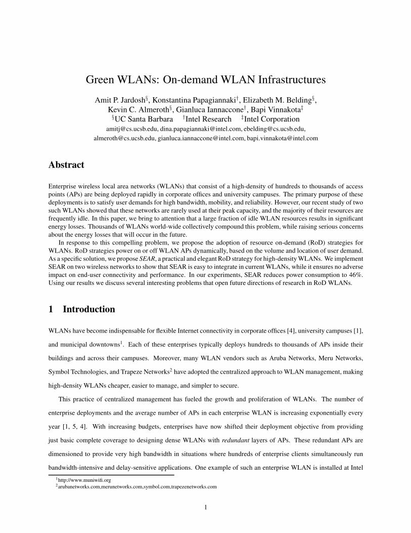
Internet
CentralController
Users
Switches
APs
Router
GRE Tunnel
Figure 1: A centralized WLAN infrastructure.
To this end, we propose and implement SEAR (Survey, Evaluate, Adapt, and Repeat), a practical policy-driven
RoD strategy for high-density WLANs. SEAR uses real online measurements to provide a necessary but sufficient set
of resources that ensures complete coverage and provides sufficient bandwidth to enterprise users. SEAR’s main ob-
jective is to maintain client connectivity and performance while reducing power wastage. SEAR can save power in any
WLAN relative to the WLAN’s usage characteristics and/or topology. In other words, on one hand, a highly redundant
WLAN with several layers of overlapping coverage that is not utilized thoroughly is a candidate for higher power sav-
ings. On the other hand, a heavily utilized network with a single layer of basic wireless coverage can save very little.
WLAN administrators can choose to adopt conservative or aggressive policies of SEAR to trade-off power savings
with client performance. Regardless of the policy chosen by individual WLAN administrators, the use of SEAR in
the thousands of WLANs will collectively save a significant volume of energy. SEAR is the first step towards saving
energy in WLANs and opens several new research directions, as discussed in Section 6.
In a position paper we published earlier [10], we identified the power wastage problem in high-density WLANs
and estimated the power savings from a simple distance-based clustering algorithm implemented in a custom Perl
simulator. In this paper, we significantly extend our initial proposal, with the following specific contributions:
• Detailed discussion of the problem of energy wastage in large-scale WLANs due to the hundreds to thousands
of idle APs world-wide.
• Description of resource management strategies for power conservation in WLANs and the impact of design
choices.
• The design of a new practical policy-driven RoD strategy called SEAR. SEAR uses measurements to dynami-
cally power on or off WLAN APs based on the location and volume of user demand, and manages user associ-
ations to ensure complete coverage and sufficient bandwidth to users.
• Demonstration of SEAR’s deployment feasibility through its implementation on two wireless networks in our
department building, using simple modifications to the current WLAN AP device drivers and network architec-
ture.
• Determination of SEAR’s deployment success through the study of three key metrics: coverage, client perfor-
mance, and client (re-)associations.
3
2 High-density WLANs
In this section we discuss the architecture of a typical high-density, centralized WLAN. We present case studies of two
enterprise WLANs, highlighting their active and idle usage patterns. These case studies show that enterprise WLANs
in different scenarios experience significant idle times. Because of these idle times, a RoD strategy such as SEAR can
be used to save energy.
2.1 Architecture
0 1 2 3 40
20
40
60
80
100
Time (Week)
Per
cent
age
of id
le A
Ps
(a) Percentage idle APs in Intel WLAN.
0 1 2 3 4 50
20
40
60
80
100
Time (Week)
Per
cent
age
of id
le A
Ps
(b) Percentage idle APs in Dartmouth WLAN.
0
0.1
0.2
0.3
0.4
0.5
0.6
0.7
0.8
0.9
1
AP idle time (Minutes)
CC
DF
(P
[X >
x])
Intel WLANDartmouth WLAN
1 hour
1 day
1 2 3 4 510 10 1010 10
(c) AP idle times in both WLANs.
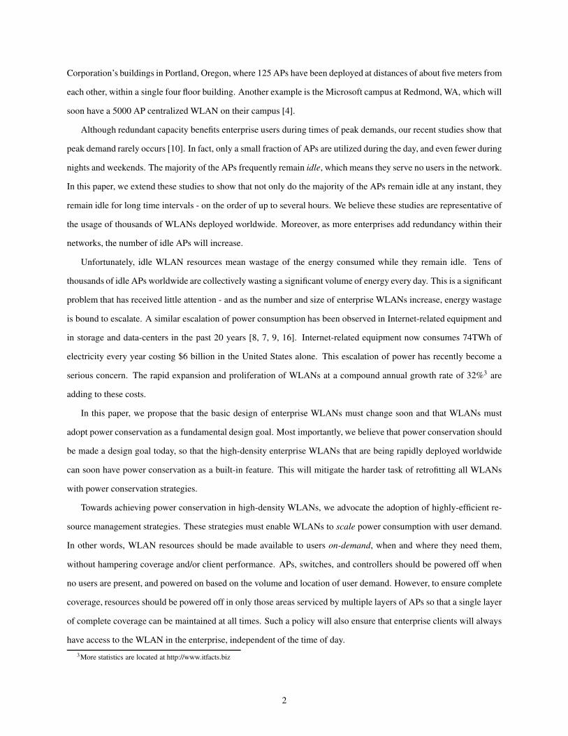
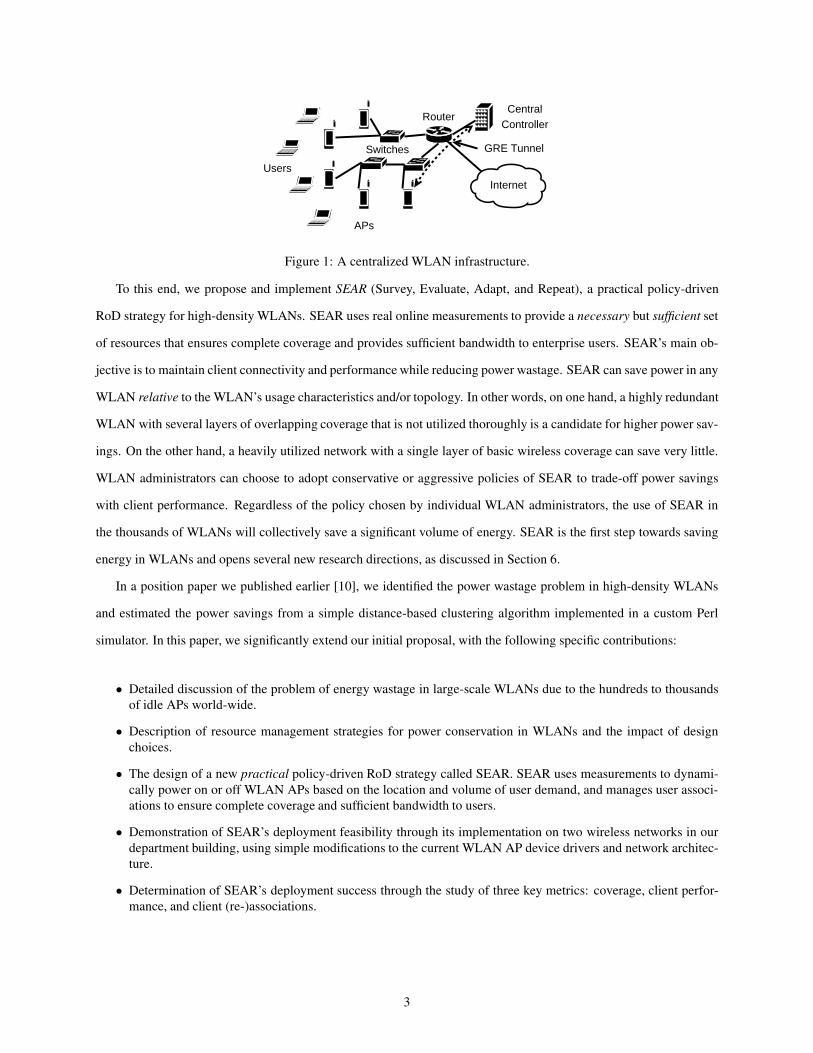
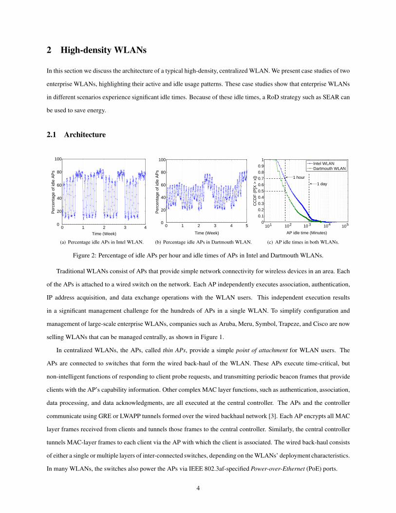
Figure 2: Percentage of idle APs per hour and idle times of APs in Intel and Dartmouth WLANs.
Traditional WLANs consist of APs that provide simple network connectivity for wireless devices in an area. Each
of the APs is attached to a wired switch on the network. Each AP independently executes association, authentication,
IP address acquisition, and data exchange operations with the WLAN users. This independent execution results
in a significant management challenge for the hundreds of APs in a single WLAN. To simplify configuration and
management of large-scale enterprise WLANs, companies such as Aruba, Meru, Symbol, Trapeze, and Cisco are now
selling WLANs that can be managed centrally, as shown in Figure 1.
In centralized WLANs, the APs, called thin APs, provide a simple point of attachment for WLAN users. The
APs are connected to switches that form the wired back-haul of the WLAN. These APs execute time-critical, but
non-intelligent functions of responding to client probe requests, and transmitting periodic beacon frames that provide
clients with the AP’s capability information. Other complex MAC layer functions, such as authentication, association,
data processing, and data acknowledgments, are all executed at the central controller. The APs and the controller
communicate using GRE or LWAPP tunnels formed over the wired backhaul network [3]. Each AP encrypts all MAC
layer frames received from clients and tunnels those frames to the central controller. Similarly, the central controller
tunnels MAC-layer frames to each client via the AP with which the client is associated. The wired back-haul consists
of either a single or multiple layers of inter-connected switches, depending on the WLANs’ deployment characteristics.
In many WLANs, the switches also power the APs via IEEE 802.3af-specified Power-over-Ethernet (PoE) ports.
4
2.2 Redundancy
The objective of enterprise WLAN deployments has moved beyond just ensuring basic coverage to all areas of the
enterprise. Now, enterprise WLANs provide several additional, or redundant layers of non-interfering APs with
overlapping coverage areas. Such redundant layers of APs provide sufficient capacity for high bandwidth demands
and also protect the network against faults and failures. The number of redundant layers of APs varies based on the
usage characteristics, design policies, and budget restrictions of the enterprise.
2.3 Case Studies
In this section we present case studies from two different large-scale enterprise WLANs. The first WLAN, deployed
inside a building of the Intel Corporation in Oregon, consists of 125 APs deployed on four adjacent floors of a single
building. Each floor of the building is 80 meters × 38 meters. The APs are deployed such that one AP serves four
to six office cubicles in the immediate proximity of the AP. This results in a high-density of APs in the building.
The WLAN’s purpose is to provide sufficient capacity for the four closest users using voice, data and multimedia
applications simultaneously. The second WLAN, deployed on the Dartmouth college campus [1], consists of 500 APs
spread across 188 buildings in a 4 km× 5 km area. The purpose of this WLAN is to provide basic Internet connectivity
to users.
To understand the usage patterns of the APs in each WLAN, we use Simple Network Management Protocol
(SNMP) logs collected from each AP at 5-minute intervals for a period of one month in June 2006 for the Intel
WLAN and November 2004 for the Dartmouth WLAN [13]. Each SNMP log contains a record of the number of users
associated with the AP, and the number of traffic bytes sent and received between each user and the AP. We use this
information to compute two metrics, the percentage of idle APs and the idle AP duration, to better understand the
usage characteristics of the APs in both WLANs.
Percentage of idle APs: WLAN APs are considered idle when no users are associated with the APs and therefore
the APs are not sending or receiving data traffic. We compute the percentage of idle APs throughout each time interval
out of all APs in each WLAN using the SNMP logs. Figures 2(a) and 2(b) show the percentage of idle APs per hour in
WLANs A and B. The peaks and troughs in the figures indicate night and day times, respectively. We observe that 10
to 80% of the APs in the Intel WLAN are idle during the month, whereas 20 to 65% of the APs are idle in Dartmouth
WLAN. A smaller percentage of Dartmouth WLAN APs remain idle because of its lower density of APs; users have
fewer choices of APs for association. As a result, an AP is more likely to be used by one or more users.
AP idle duration: The AP idle duration metric indicates how long each AP remains idle before at least a single
user associates with the AP. Using SNMP logs from both WLANs, we show in Figure 2(c) the CCDF of the lengths
of time each AP remains idle during the data collection period of 1-month. We observe that more than 70% of the
5
Intel WLAN APs are idle for more than 60 contiguous minutes, while more than 50% of the Dartmouth WLAN APs
are idle for more than 60 minutes. Some of the APs remain idle for more than a full day. These idle times can also be
attributed to nights and weekends when few or no users associate with the APs.
2.4 Power Consumption: How much?
In centralized WLANs, the three main consumers of energy are APs, switches, and controllers. Each AP typically
draws up to 10W power from PoE ports on PoE-compatible switches, from the 15.4W allocated per port by PoE
specifications. Each WLAN switch, with 24 to 72 PoE ports, consumes up to 350W each per hour. This consumption
of 350W is in addition to the power the switches supply to the APs connected to them. Commercial central controllers
of centralized WLANs provided by Aruba, Meru, Trapeze, Symbol, and Cisco, that can manage up to 512 APs and
8192 users, consume up to 466W.
Based on these numbers alone, 100 APs consume about 8.76 MWh of energy per year. Such energy consumption
in tens of thousands of APs is far from negligible even today - and will continue to increase as WLAN densities
increase.
2.5 Power Wastage: Does it matter?
Today, 74TWh of electricity is consumed by Internet-related equipment installed in the United States alone [8]. This
consumption of energy has increased dramatically only in the past 20 years. Research institutions and universities
are currently devising techniques to reduce consumption in such networks and devices. Similar trends in the wireless
networking industry are adding to this power consumption. The enterprise WLAN market is growing at the compound
annual growth rate of 32%4, with more than 50% of the organizations in the US deploying WLANs. Because WLANs
are known to increase work productivity, enterprises are investing in denser deployments of WLAN APs. Aruba
Networks, the leading WLAN vendor, has reported acquiring 100 new customers for their centralized WLANs per
quarter, with an average of 75 APs per WLAN5. Tropos, a leading wireless mesh network vendor, has deployed more
than 500 mesh networks in city downtowns and other municipal areas with hundreds of routers6. As millions of dollars
are spent on dense WLAN deployments, the aggregate power wasted in each of those WLANs will rapidly increase
since they are unlikely to be used at their peak capacity at all times.
4http://www.itfacts.biz/5http://www.arubanetworks.com/ company/press/2005/07/186http://www.tropos.com
6
2.6 Power Conservation: Why now?
We believe that serious steps need to be taken as soon as possible to reduce energy consumption before more access
points and routers are deployed around the world. If energy conservation is not given a serious thought today, wireless
devices will continue to waste energy. Moreover, rewiring a four-storey building costs five times more than a new
deployment itself7. As a result, a significant amount of power could be saved if WLANs were designed with power
conservation as a design goal [10].
While wireless networks of different usage characteristics are likely to save different volumes of energy, we believe
that any power savings within a network will contribute to large cumulative savings worldwide. For that matter, even
if all the wireless access points deployed in homes adopt power conservation strategies, the cumulative savings will
be enormous. Power conservation in WLANs is similar to the Energy Star initiative where close to negligible savings
within 300 million household products have cumulatively saved $14 billion in the year 2006 alone 8.
3 Resource On-demand WLANs
To reduce the unnecessary wastage of energy in large-scale and high-density WLANs, we introduce the notion of
Resource On-Demand (RoD) WLANs. The main objective of RoD WLANs is to efficiently manage WLAN resources
to save energy while ensuring scenario-specific end-user performance guarantees. When user demand is scarce, RoD
WLANs reduce resource redundancy by strategically powering off WLAN resources (APs, switches, and routers).
As a result, WLAN coverage is still maintained; only redundant coverage is reduced. When user demand increases,
WLAN resources are powered on to scale resource and coverage redundancy proportionately. In high-density WLANs,
RoD strategies will thus reduce energy wastage without adversely impacting coverage and end-user performance.
3.1 RoD Strategy Classes
RoD WLANs can adopt two different classes of operating strategies, as described below.
Demand-driven: Using demand-driven RoD strategies, WLANs can power on or off resources based on the user
demand assessed by the WLAN at a given time. The determination of demand is based on the computation of one
or more appropriate parameters, such as the number of active users in the network and the volume of offered traffic
load. In typical demand-driven strategies, the WLAN’s central controller periodically collects information from the
APs, estimates user demand using scenario-specific parameters, and then computes the best set of APs, switches, and
routers that will satisfy the estimated user demand. The advantage of these strategies is that the WLAN can, at all
times, ensure high energy savings and satisfy end-user performance. However, the trade-off is in the overhead of
7http://www.arubanetworks.com/technology/8http://www.energystar.gov/
7
assessing user demands and continuously reconfiguring the APs. Therefore, demand-driven strategies are suitable in
scenarios where the user demand may vary significantly over time. For instance, demand-driven RoD strategies may
be used on university campuses wherein user demand is expected to vary significantly on a daily, as well as seasonal,
basis.
Schedule-driven: Schedule-driven RoD strategies use pre-determined schedules to power on and off specific
WLAN resources. These schedules can either be determined from WLAN historical usage patterns or can be based
on the administrators’ experience. The advantage of using schedules stems from their minimal processing overhead.
However, the trade-off is that they fail to power on or off the necessary and sufficient set of resources during times
of unexpected change in user demand. As a result, schedule-driven solutions are suitable for scenarios where user
demand is closely predictable. For instance, during most conferences and meetings, schedules are predetermined and
users are expected to primarily be present during meeting times [11]. In such scenarios, network managers may decide
to power all the APs before a meeting begins and power all of them off shortly after the meeting is over.
3.2 RoD WLAN Design Requirements
To ensure the successful adoption of RoD solutions in today’s WLANs, both classes of RoD strategies should follow
a set of design requirements. These requirements allow RoD strategies to achieve their objective of conserving energy
without adversely impacting end-user performance. The requirements for an RoD strategy are the following:
Requirement 1: Ensure coverage: A good RoD strategy is required to maintain the same coverage as its always-on
counterpart. In other words, powering off APs must not create coverage holes where users cannot receive service.
Requirement 2: Maintain client performance: A good RoD strategy should offer the same service to clients even
when part of the infrastructure is off. Client service levels can be maintained by avoiding WLAN topologies in which
clients are far away from their closest AP or in which an AP is required to support so many clients that congestion
occurs. Within such topologies, clients may experience an increase in packet loss or reduction in the sustainable
transmission rate due to weak wireless links or congestion. A good RoD strategy should be able to deliver performance
equivalent to that of an always-on network.
Requirement 3: Avoid frequent client re-associations: The powering on and off of WLAN APs by RoD strategies
can force clients to change their associations between APs. Frequent re-associations are undesirable because re-
association delays can break clients’ traffic flows and thereby impact their performance. A good RoD strategy should
avoid frequent client disconnections from the WLAN.
Based on these requirements, we develop a RoD strategy called Survey, Evaluate, Adapt, and Repeat (SEAR). In
the following section, we discuss in detail the design of SEAR, and feasibility of deploying SEAR in current WLANs.
8
�Topology ManagementPower on or off APs
based on estimated demand [Section 4.3]
Demand EstimationEstimate user traffic volume
and/or performance [Section 4.2]
�User Management(Re-)Associate clients
based on topology changes [Section 4.4]
Green ClusteringForm AP clusters
& select the cluster-lead APs[Section 4.1]
SEAR
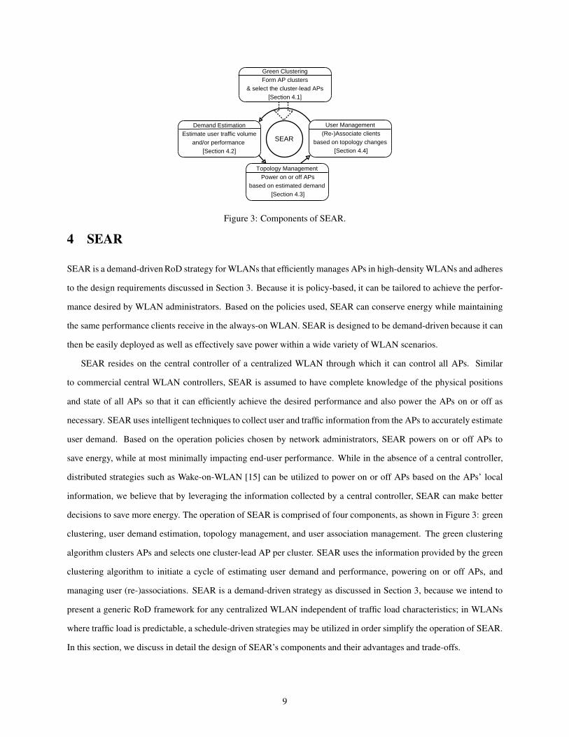
Figure 3: Components of SEAR.
4 SEAR
SEAR is a demand-driven RoD strategy for WLANs that efficiently manages APs in high-density WLANs and adheres
to the design requirements discussed in Section 3. Because it is policy-based, it can be tailored to achieve the perfor-
mance desired by WLAN administrators. Based on the policies used, SEAR can conserve energy while maintaining
the same performance clients receive in the always-on WLAN. SEAR is designed to be demand-driven because it can
then be easily deployed as well as effectively save power within a wide variety of WLAN scenarios.
SEAR resides on the central controller of a centralized WLAN through which it can control all APs. Similar
to commercial central WLAN controllers, SEAR is assumed to have complete knowledge of the physical positions
and state of all APs so that it can efficiently achieve the desired performance and also power the APs on or off as
necessary. SEAR uses intelligent techniques to collect user and traffic information from the APs to accurately estimate
user demand. Based on the operation policies chosen by network administrators, SEAR powers on or off APs to
save energy, while at most minimally impacting end-user performance. While in the absence of a central controller,
distributed strategies such as Wake-on-WLAN [15] can be utilized to power on or off APs based on the APs’ local
information, we believe that by leveraging the information collected by a central controller, SEAR can make better
decisions to save more energy. The operation of SEAR is comprised of four components, as shown in Figure 3: green
clustering, user demand estimation, topology management, and user association management. The green clustering
algorithm clusters APs and selects one cluster-lead AP per cluster. SEAR uses the information provided by the green
clustering algorithm to initiate a cycle of estimating user demand and performance, powering on or off APs, and
managing user (re-)associations. SEAR is a demand-driven strategy as discussed in Section 3, because we intend to
present a generic RoD framework for any centralized WLAN independent of traffic load characteristics; in WLANs
where traffic load is predictable, a schedule-driven strategies may be utilized in order simplify the operation of SEAR.
In this section, we discuss in detail the design of SEAR’s components and their advantages and trade-offs.
9
E D
A
B
C
(a) (b)
C
DE
A
B
AP coverage regions Cluster coverage region
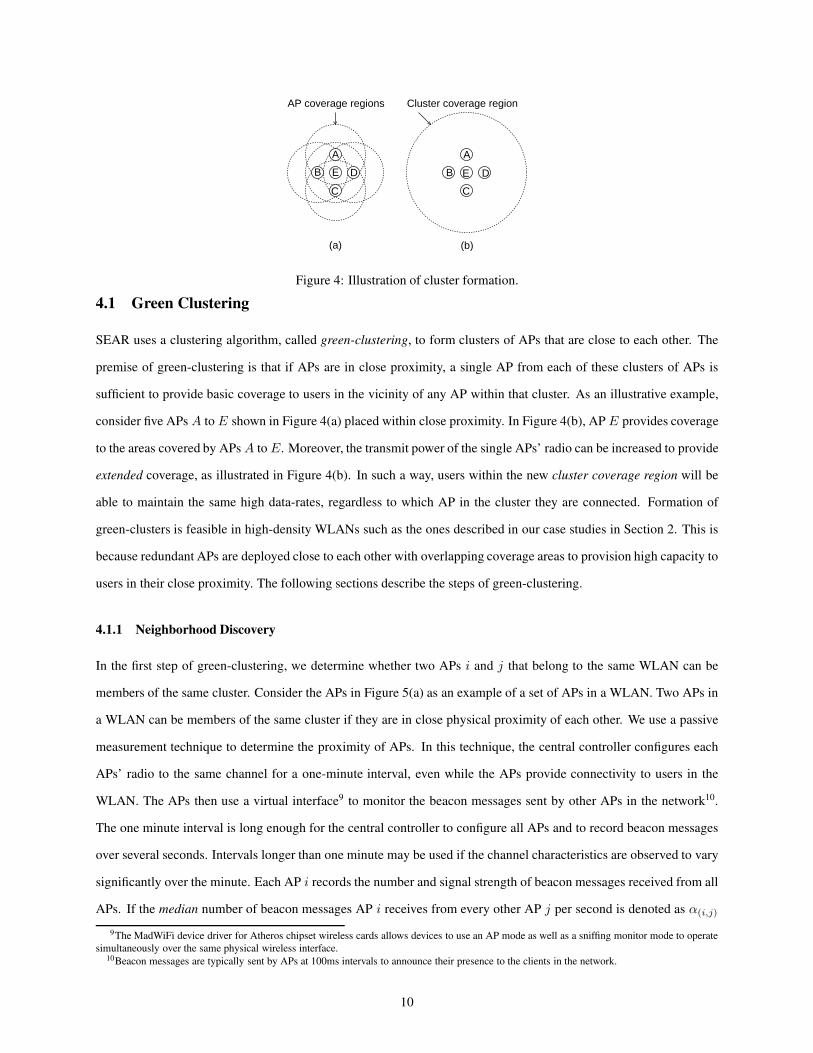
Figure 4: Illustration of cluster formation.
4.1 Green Clustering
SEAR uses a clustering algorithm, called green-clustering, to form clusters of APs that are close to each other. The
premise of green-clustering is that if APs are in close proximity, a single AP from each of these clusters of APs is
sufficient to provide basic coverage to users in the vicinity of any AP within that cluster. As an illustrative example,
consider five APs A to E shown in Figure 4(a) placed within close proximity. In Figure 4(b), AP E provides coverage
to the areas covered by APs A to E. Moreover, the transmit power of the single APs’ radio can be increased to provide
extended coverage, as illustrated in Figure 4(b). In such a way, users within the new cluster coverage region will be
able to maintain the same high data-rates, regardless to which AP in the cluster they are connected. Formation of
green-clusters is feasible in high-density WLANs such as the ones described in our case studies in Section 2. This is
because redundant APs are deployed close to each other with overlapping coverage areas to provision high capacity to
users in their close proximity. The following sections describe the steps of green-clustering.
4.1.1 Neighborhood Discovery
In the first step of green-clustering, we determine whether two APs i and j that belong to the same WLAN can be
members of the same cluster. Consider the APs in Figure 5(a) as an example of a set of APs in a WLAN. Two APs in
a WLAN can be members of the same cluster if they are in close physical proximity of each other. We use a passive
measurement technique to determine the proximity of APs. In this technique, the central controller configures each
APs’ radio to the same channel for a one-minute interval, even while the APs provide connectivity to users in the
WLAN. The APs then use a virtual interface9 to monitor the beacon messages sent by other APs in the network10.
The one minute interval is long enough for the central controller to configure all APs and to record beacon messages
over several seconds. Intervals longer than one minute may be used if the channel characteristics are observed to vary
significantly over the minute. Each AP i records the number and signal strength of beacon messages received from all
APs. If the median number of beacon messages AP i receives from every other AP j per second is denoted as α(i,j)
9The MadWiFi device driver for Atheros chipset wireless cards allows devices to use an AP mode as well as a sniffing monitor mode to operate
simultaneously over the same physical wireless interface.10Beacon messages are typically sent by APs at 100ms intervals to announce their presence to the clients in the network.
10
(a) (b)
(c) (d)
2 4 2
3
1 1
3
1
1
2
0
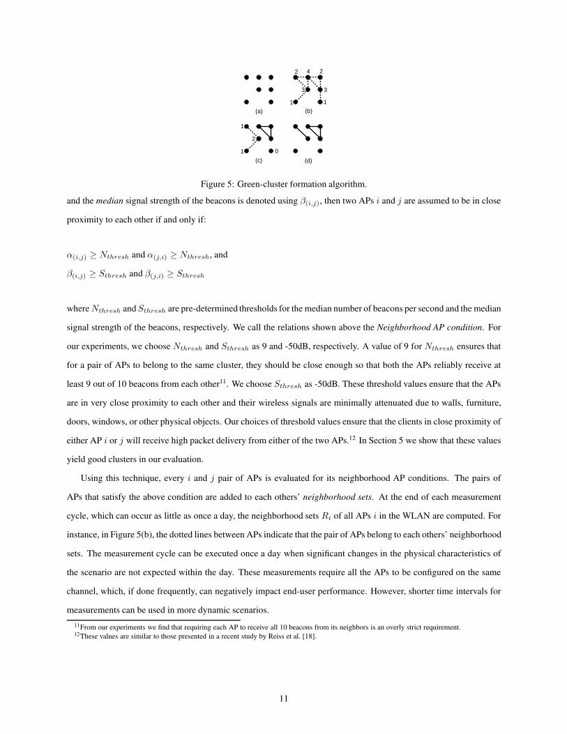
Figure 5: Green-cluster formation algorithm.
and the median signal strength of the beacons is denoted using β(i,j), then two APs i and j are assumed to be in close
proximity to each other if and only if:
α(i,j) ≥ Nthresh and α(j,i) ≥ Nthresh, and
β(i,j) ≥ Sthresh and β(j,i) ≥ Sthresh
where Nthresh and Sthresh are pre-determined thresholds for the median number of beacons per second and the median
signal strength of the beacons, respectively. We call the relations shown above the Neighborhood AP condition. For
our experiments, we choose Nthresh and Sthresh as 9 and -50dB, respectively. A value of 9 for Nthresh ensures that
for a pair of APs to belong to the same cluster, they should be close enough so that both the APs reliably receive at
least 9 out of 10 beacons from each other11. We choose Sthresh as -50dB. These threshold values ensure that the APs
are in very close proximity to each other and their wireless signals are minimally attenuated due to walls, furniture,
doors, windows, or other physical objects. Our choices of threshold values ensure that the clients in close proximity of
either AP i or j will receive high packet delivery from either of the two APs.12 In Section 5 we show that these values
yield good clusters in our evaluation.
Using this technique, every i and j pair of APs is evaluated for its neighborhood AP conditions. The pairs of
APs that satisfy the above condition are added to each others’ neighborhood sets. At the end of each measurement
cycle, which can occur as little as once a day, the neighborhood sets Ri of all APs i in the WLAN are computed. For
instance, in Figure 5(b), the dotted lines between APs indicate that the pair of APs belong to each others’ neighborhood
sets. The measurement cycle can be executed once a day when significant changes in the physical characteristics of
the scenario are not expected within the day. These measurements require all the APs to be configured on the same
channel, which, if done frequently, can negatively impact end-user performance. However, shorter time intervals for
measurements can be used in more dynamic scenarios.
11From our experiments we find that requiring each AP to receive all 10 beacons from its neighbors is an overly strict requirement.12These values are similar to those presented in a recent study by Reiss et al. [18].
11
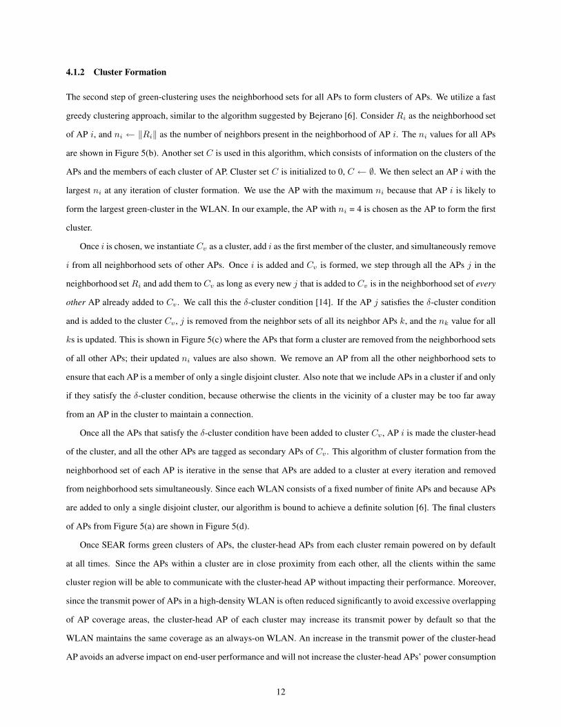
4.1.2 Cluster Formation
The second step of green-clustering uses the neighborhood sets for all APs to form clusters of APs. We utilize a fast
greedy clustering approach, similar to the algorithm suggested by Bejerano [6]. Consider Ri as the neighborhood set
of AP i, and ni ← ‖Ri‖ as the number of neighbors present in the neighborhood of AP i. The ni values for all APs
are shown in Figure 5(b). Another set C is used in this algorithm, which consists of information on the clusters of the
APs and the members of each cluster of AP. Cluster set C is initialized to 0, C ← ∅. We then select an AP i with the
largest ni at any iteration of cluster formation. We use the AP with the maximum ni because that AP i is likely to
form the largest green-cluster in the WLAN. In our example, the AP with ni = 4 is chosen as the AP to form the first
cluster.
Once i is chosen, we instantiate Cv as a cluster, add i as the first member of the cluster, and simultaneously remove
i from all neighborhood sets of other APs. Once i is added and Cv is formed, we step through all the APs j in the
neighborhood set Ri and add them to Cv as long as every new j that is added to Cv is in the neighborhood set of every
other AP already added to Cv . We call this the δ-cluster condition [14]. If the AP j satisfies the δ-cluster condition
and is added to the cluster Cv , j is removed from the neighbor sets of all its neighbor APs k, and the nk value for all
ks is updated. This is shown in Figure 5(c) where the APs that form a cluster are removed from the neighborhood sets
of all other APs; their updated ni values are also shown. We remove an AP from all the other neighborhood sets to
ensure that each AP is a member of only a single disjoint cluster. Also note that we include APs in a cluster if and only
if they satisfy the δ-cluster condition, because otherwise the clients in the vicinity of a cluster may be too far away
from an AP in the cluster to maintain a connection.
Once all the APs that satisfy the δ-cluster condition have been added to cluster Cv , AP i is made the cluster-head
of the cluster, and all the other APs are tagged as secondary APs of Cv . This algorithm of cluster formation from the
neighborhood set of each AP is iterative in the sense that APs are added to a cluster at every iteration and removed
from neighborhood sets simultaneously. Since each WLAN consists of a fixed number of finite APs and because APs
are added to only a single disjoint cluster, our algorithm is bound to achieve a definite solution [6]. The final clusters
of APs from Figure 5(a) are shown in Figure 5(d).
Once SEAR forms green clusters of APs, the cluster-head APs from each cluster remain powered on by default
at all times. Since the APs within a cluster are in close proximity from each other, all the clients within the same
cluster region will be able to communicate with the cluster-head AP without impacting their performance. Moreover,
since the transmit power of APs in a high-density WLAN is often reduced significantly to avoid excessive overlapping
of AP coverage areas, the cluster-head AP of each cluster may increase its transmit power by default so that the
WLAN maintains the same coverage as an always-on WLAN. An increase in the transmit power of the cluster-head
AP avoids an adverse impact on end-user performance and will not increase the cluster-head APs’ power consumption
12
significantly either. In the next step of SEAR, we explain how other secondary APs are powered on within clusters
based on the location and estimated volume of user demand in the network.
4.1.3 Trade-offs of Clustering Thresholds
SEAR’s measurements-based technique of forming green clusters ensures that APs that form clusters are in close
proximity of each other. The constraints on the closeness of the APs can be varied based on thresholds of signal
attenuation Sthresh and packet loss rate Nthresh between APs. The choice of thresholds is a trade-off between power
savings and client performance. In other words, low thresholds are indicative of closer proximity between APs, which
means smaller sizes of clusters, smaller power savings, but better client performance. Conversely, higher thresholds
relax the clustering constraints, which results in larger clusters and more power savings - although, client performance
may deteriorate. Based on the acceptable performance bounds of WLANs, administrators can individually choose
their thresholds and thereby control the relative power savings within their WLANs. In Section 5 of this paper, we use
low thresholds of 9 and -50 dB to ensure that APs that are extremely close to each other are clustered.
4.2 Demand Estimation
One of the foremost tasks of any demand-driven RoD strategy is user demand estimation within each green-cluster.
User demand estimation assists SEAR in making strategic decisions to power on or off the WLAN APs within each
cluster. An accurate estimate of user demand is helpful in maintaining client performance, while achieving significant
power savings.
The accuracy of the estimate is determined by a set of metrics as well as the usage characteristics of the WLAN.
For instance, the count of users in a cluster is a simple metric to estimate user demand. However, the problem with a
simple count of users is that it can over- or under-estimate user demand within a cluster if many users generate little
traffic or few users generate heavy traffic load, respectively. Alternatively, a metric such as the data-rates of frames
sent by clients can be used because low frame data-rates indicate the occurrence of frame collisions due to heavy traffic
load within the cluster. Unfortunately, frame data-rates are not a direct measure of the user demand in the network.
In this paper we use channel utilization (channel busy time) to estimate user demand [12, 19], because it encom-
passes the user demand estimation properties of user count as well as data-rates. Channel utilization is defined as the
percentage of time the medium remains busy due to the transmission of bytes in the network or due to inter-frame
spacings.
Each AP in the WLAN continuously sniffs MAC layer data and control frames transmitted by all the clients
and APs in its vicinity on the same channel, and computes both the aggregate channel utilization of the medium in the
vicinity of each AP, and the channel utilization per client connected to that AP [12]. Since the MadWifi wireless device
13
drivers for Atheros wireless cards allow a single radio interface to be configured in AP mode as well as monitor mode,
the APs may sniff traffic without interrupting or impacting AP operations. The APs periodically send their computed
channel utilization values to SEAR’s central controller, along with the count of the number of clients associated with
the AP and the channel utilization values for each client connected to that AP.
Using all this information sent by APs in the WLAN, SEAR establishes the area in the network with excess
demand, based on the cluster to which the APs belong, and the volume of user demand based on the channel utilization
metric values computed at each AP. In the next step, we describe how SEAR uses this channel utilization information
to power on and off APs in the WLAN.
4.3 Topology Management
At regular reconfiguration intervals Ireconf , SEAR uses the information on channel utilization values per AP and the
number of clients connected to an AP to power on or off secondary APs within a cluster. If the aggregate channel
utilization value at any AP i exceeds a pre-configured trigger threshold Tthresh and the number of clients connected
to that AP is greater than one, SEAR powers on an additional secondary AP within i’s the cluster. The intuition
behind this policy is that if more than a single client causes the aggregate channel utilization at an AP i to increase to
a value greater than Tthresh, then the cluster of APs to which i belongs experiences excess traffic load. As a result,
SEAR should power on another AP within the same cluster so that the clients have an additional AP to which they can
connect. If the number of clients connected to the AP is one, then powering on an additional AP will not reduce the
load per AP because a single user’s load cannot be distributed between two APs13.
Once the secondary AP within the same cluster is powered on, SEAR ensures that the APs within the same cluster
are configured to appropriate channels, that minimize overlap. SEAR distributes the load from the clients between all
the APs within the cluster so that the clients receive better performance, as described in the following section. If a
secondary AP in the WLAN does not have any clients connected to it for an interval of Tidle, the AP reports this to
SEAR’s central controller. The central controller powers off this AP so that power can be saved.
Transmit power settings: The transmit powers of APs in high-density WLANs are often decreased in order to
service clients only in their close vicinity. An RoD strategy such as SEAR can therefore increase the transmit power
of APs when fewer APs per cluster are powered on, and decrease the power as more APs are utilized. A detailed
algorithm for transmit power control in RoD WLANs is not discussed in this paper, and forms interesting future work.
In our experiments, we maintain the transmit power of all APs to their radios’ maximum of 19 dBm (= 79mW) at all
times.
13Note that a client in the WLAN is identified by the unique MAC address of its device’s wireless interface. As a result, devices with more than
one wireless interface will be considered as more than one client.
14
In the following section we discuss the technique SEAR uses to distribute users and load within APs of a cluster
once it powers on or off a secondary AP.
4.4 User Management
As discussed in Section 3, one of the requirements of a RoD strategy such as SEAR is to reduce association instability
and maintain client performance. Because of this requirement, SEAR carefully manages the association of users
within the WLAN by reducing excessive roaming of users between APs. SEAR proactively switches clients between
APs in a cluster of APs to balance the load detected within a cluster so that each client in the cluster experiences better
performance.
Load balancing: At Ireconf intervals, SEAR powers on an additional AP within a cluster if any AP within the
cluster reports “overload” to the controller. Let us call the aggregate channel utilization reported by an AP i as Ui; the
number of clients connected with the same AP i as Ni; and the channel utilization per client c connected with an AP i
as Pc,i. SEAR’s central controller generates a sorted list of clients per AP i based on the Pc,i values.
The SEAR central controller’s next step is to move half the load from AP i to the new AP, say, AP j. SEAR moves
half the load to the new AP in order to evenly balance the load between the two APs so that the clients connected with
either AP experience an equally better performance. To achieve this movement of load, SEAR iteratively moves the
client with the greatest traffic load in the sorted list of clients from AP i to AP j. As the SEAR controller moves a
client to the new AP j, it updates the aggregate utilization of AP i by subtracting the per-client channel utilization of
that client. The new aggregate channel utilization for AP i after the subtraction is denoted as U ′
i , and utilization on
AP j is denoted as Uj . SEAR continues to move clients from AP i to AP j until: U ′
i ≤12 × Ui and Uj ≤ Tthresh.
If a move of a user from i to j leads to the violation of the second condition, then we proceed down the ranked list
until we satisfy the terminating condition. The SEAR central controller repeats this process of balancing load for all
the APs that report an aggregate channel utilization value greater than Tthresh. SEAR chooses to move the topmost
client in the sorted list first because such a move is likely to cause the fewest number of clients to handoff from one
AP to another. This strategy thus complies with the requirement of an RoD strategy avoiding significant association
instability.
We use the above load diversion strategy because it satisfies the third requirement of a good RoD strategy and is
easy to implement and deploy. However, the design and implementation of more efficient load diversion mechanisms
is interesting future work.
Enforcing user association: SEAR uses access control black lists to enforce a client handoff between APs. The
MadWifi Atheros chipset wireless driver allows an AP to use such black lists of MAC addresses of clients. If the MAC
address of a client is present in that list, the AP will not allow the client to associate with it. The advantage of using
15
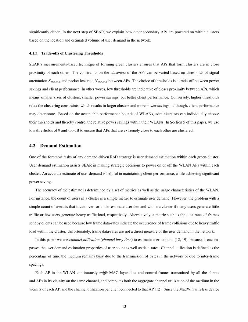
Figure 6: The floor map of two adjacent floors of our building, indicating the locations of APs, cluster-head APs, and
clients.
black-lists on APs is that the clients are forced to associate with only those APs on which they are not black-listed. As
a client is moved from an AP i to AP j, the client is added to AP i’s black-list. This forces the client to disconnect
from AP i and associate with the new AP j.
While a black list-based strategy was effective in re-associating users in our implementation of SEAR, we could
replace it by using the upcoming IEEE 802.11v [2] standard where APs can explicitly ask users to re-associate with
an alternate AP.
5 Evaluation
In this section we first justify the use of a centralized RoD strategy through the evaluation of a simple distributed
strategy. Our evaluation demonstrates the weaknesses of a distributed approach. We then implement and evaluate
SEAR in two wireless networks to show that it satisfies the three requirements of a good RoD strategy. The main
objectives of implementing SEAR in real networks are to: (a) understand the effectiveness of implementing green
clustering within current wireless devices; (b) study the impact of green clustering on end-user performance; and (c)
evaluate the feasibility of user and topology management strategies to successfully power on and off APs for energy
savings under realistic traffic conditions.
5.1 Sniff-n-Sleep RoD Strategy
To begin, we first evaluate a simple distributed strategy for RoD WLANs. We call this strategy Sniff-n-Sleep. Our
objective is to show that a simple-to-implement distributed strategy similar to Wake-on-WLAN [15] can be used to
save energy in a WLAN, but has limitations that are likely to degrade the performance achieved by clients.
16
0 10 20 30 40 50 600
0.1
0.2
0.3
0.4
0.5
0.6
0.7
0.8
0.9
1
Number of Seconds
CD
F
tsleep
= 60 seconds, tsniff
= 10 seconds
tsleep
= 60 seconds, tsniff
= 30 seconds
tsleep
= 60 seconds, tsniff
= 60 seconds
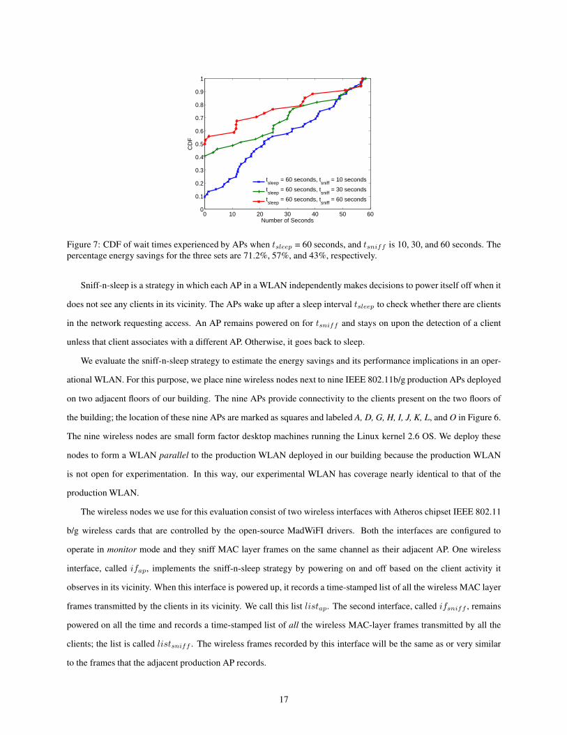
Figure 7: CDF of wait times experienced by APs when tsleep = 60 seconds, and tsniff is 10, 30, and 60 seconds. The
percentage energy savings for the three sets are 71.2%, 57%, and 43%, respectively.
Sniff-n-sleep is a strategy in which each AP in a WLAN independently makes decisions to power itself off when it
does not see any clients in its vicinity. The APs wake up after a sleep interval tsleep to check whether there are clients
in the network requesting access. An AP remains powered on for tsniff and stays on upon the detection of a client
unless that client associates with a different AP. Otherwise, it goes back to sleep.
We evaluate the sniff-n-sleep strategy to estimate the energy savings and its performance implications in an oper-
ational WLAN. For this purpose, we place nine wireless nodes next to nine IEEE 802.11b/g production APs deployed
on two adjacent floors of our building. The nine APs provide connectivity to the clients present on the two floors of
the building; the location of these nine APs are marked as squares and labeled A, D, G, H, I, J, K, L, and O in Figure 6.
The nine wireless nodes are small form factor desktop machines running the Linux kernel 2.6 OS. We deploy these
nodes to form a WLAN parallel to the production WLAN deployed in our building because the production WLAN
is not open for experimentation. In this way, our experimental WLAN has coverage nearly identical to that of the
production WLAN.
The wireless nodes we use for this evaluation consist of two wireless interfaces with Atheros chipset IEEE 802.11
b/g wireless cards that are controlled by the open-source MadWiFI drivers. Both the interfaces are configured to
operate in monitor mode and they sniff MAC layer frames on the same channel as their adjacent AP. One wireless
interface, called ifap, implements the sniff-n-sleep strategy by powering on and off based on the client activity it
observes in its vicinity. When this interface is powered up, it records a time-stamped list of all the wireless MAC layer
frames transmitted by the clients in its vicinity. We call this list listap. The second interface, called ifsniff , remains
powered on all the time and records a time-stamped list of all the wireless MAC-layer frames transmitted by all the
clients; the list is called listsniff . The wireless frames recorded by this interface will be the same as or very similar
to the frames that the adjacent production AP records.
17
We performed three sets of experiments, each for a duration of 7 days. In all experiments, we use tsleep = 60
seconds. This value is short enough to avoid long client wait times and long enough to avoid rapid powering on and
off of the AP. The problems with powering on and off APs rapidly is that it can cause several client re-associations.
We used three values of tsniff , 10, 30, and 60 seconds, for each of the three sets of experiments. The energy savings
in each experiment are computed as the percentage of time the ifap interface is powered off over the total time for the
experiment. We compare the two lists listap and listsniff for each wireless node to identify the frames ifap missed
while it was asleep. The difference twait between the time when a missed frame was detected by ifsniff and the time
at which ifap wakes up is defined as the wait time for the user in the network. We call this interval the wait time
because a wireless client may have to wait twait before it detects an AP in its vicinity.
Figure 7 shows the CDF of wait times for users for the three sets of experiments. Not surprisingly, there is a clear
trade-off between the energy savings and user wait times for all three sets of experiments. In other words, short tsniff
results in more energy savings but higher user wait times. With a short tsniff , the AP sleeps more often and does not
spend enough time checking for the presence of users. Thus, users must wait for a longer duration before they can
connect with the AP again.
The evaluation of the sniff-n-sleep strategy shows that even though energy savings can be achieved by deploying
a simple strategy, the trade-off is that users must wait up to tsleep time before they can even detect the presence of
a WLAN. This wait time negatively impacts the user experience. Based on this conclusion, we believe that a well-
coordinated strategy such as SEAR should be used to ensure complete coverage in the network and prevent long
association wait times.
5.2 Performance Evaluation of SEAR
We evaluate SEAR to ensure that it satisfies each of the three requirements of a good RoD strategy listed in Section 3.2.
Since one of the primary objectives of this paper is to understand the feasibility of implementing a RoD strategy using
current devices and software, instead of simulation, we use two wireless networks for our evaluation.
The first network is a WLAN consisting of 15 APs and nine clients deployed on two adjacent floors of our depart-
ment building. The locations of these APs are marked as black squares and labeled AP A to AP O in Figure 6; there
are six more APs deployed for this experiment than in the previous section. We deploy these extra APs to create a
denser WLAN for the rest of our evaluation. Using this network, we evaluate the impact of SEAR’s green-clustering
on WLAN coverage and client throughput, and compute the power savings achieved using SEAR.
The second network of three APs and nine client laptops is deployed within a single room. We use this network to
closely evaluate the impact of SEAR’s user association management mechanisms on the performance of a high density
of clients.
18
Clie
nt N
umbe
r
A B C D E F G H I J K L M N O
AP Label
5
6
7
8
4
3
2
1
9
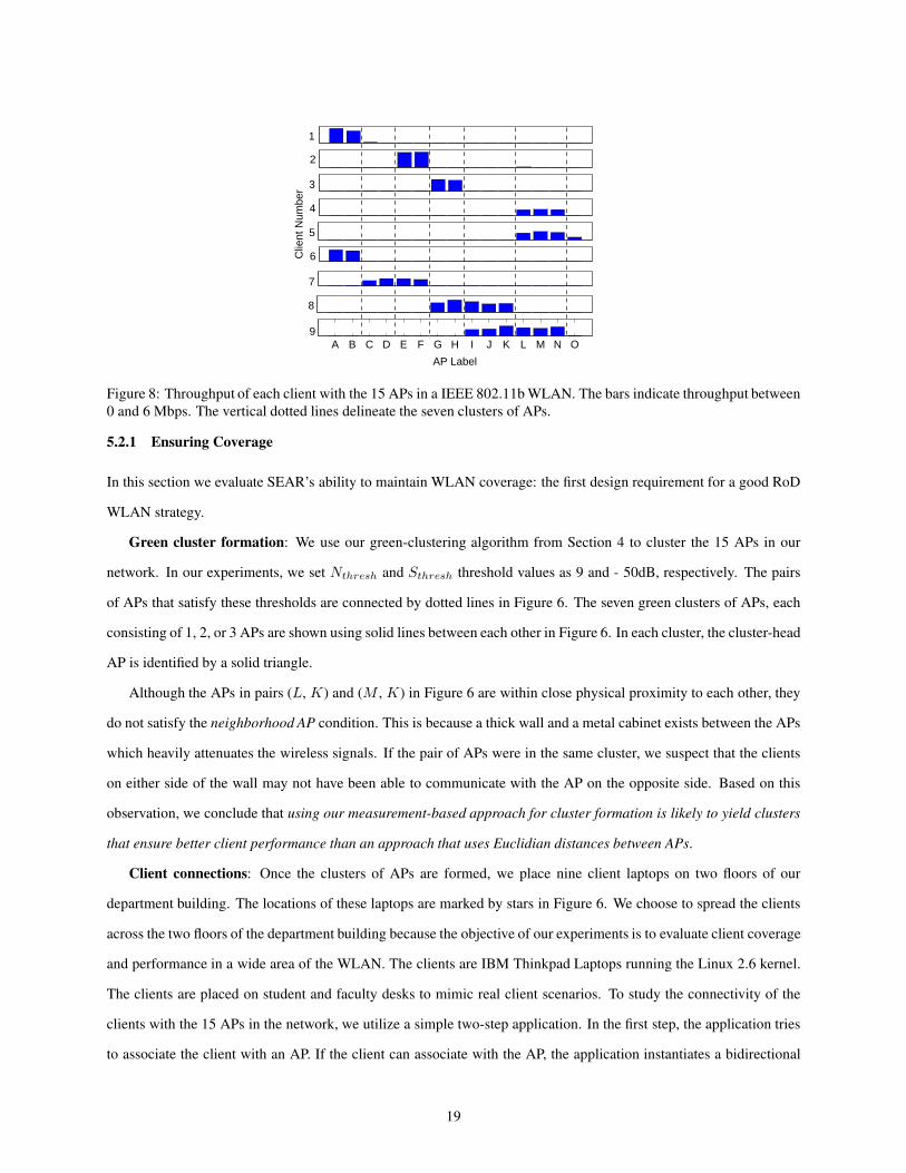
Figure 8: Throughput of each client with the 15 APs in a IEEE 802.11b WLAN. The bars indicate throughput between
0 and 6 Mbps. The vertical dotted lines delineate the seven clusters of APs.
5.2.1 Ensuring Coverage
In this section we evaluate SEAR’s ability to maintain WLAN coverage: the first design requirement for a good RoD
WLAN strategy.
Green cluster formation: We use our green-clustering algorithm from Section 4 to cluster the 15 APs in our
network. In our experiments, we set Nthresh and Sthresh threshold values as 9 and - 50dB, respectively. The pairs
of APs that satisfy these thresholds are connected by dotted lines in Figure 6. The seven green clusters of APs, each
consisting of 1, 2, or 3 APs are shown using solid lines between each other in Figure 6. In each cluster, the cluster-head
AP is identified by a solid triangle.
Although the APs in pairs (L, K) and (M , K) in Figure 6 are within close physical proximity to each other, they
do not satisfy the neighborhood AP condition. This is because a thick wall and a metal cabinet exists between the APs
which heavily attenuates the wireless signals. If the pair of APs were in the same cluster, we suspect that the clients
on either side of the wall may not have been able to communicate with the AP on the opposite side. Based on this
observation, we conclude that using our measurement-based approach for cluster formation is likely to yield clusters
that ensure better client performance than an approach that uses Euclidian distances between APs.
Client connections: Once the clusters of APs are formed, we place nine client laptops on two floors of our
department building. The locations of these laptops are marked by stars in Figure 6. We choose to spread the clients
across the two floors of the department building because the objective of our experiments is to evaluate client coverage
and performance in a wide area of the WLAN. The clients are IBM Thinkpad Laptops running the Linux 2.6 kernel.
The clients are placed on student and faculty desks to mimic real client scenarios. To study the connectivity of the
clients with the 15 APs in the network, we utilize a simple two-step application. In the first step, the application tries
to associate the client with an AP. If the client can associate with the AP, the application instantiates a bidirectional
19
UDP flow. The UDP flow is used to compute the average throughput of the link between the client and the AP. The
same application is used to iteratively compute the throughput between each of the nine clients and 15 APs.
Figure 8 shows the throughput of all the nine clients with the 15 APs. Each bar is a value between 0 and 6 Mbps
and represents the client’s throughput to the AP. The vertical dashed lines delineate the clusters of APs. We utilize
the throughput received by a client as a metric for evaluation because throughput quantifies the quality of the clients’
connections with the WLAN.
We make three key observations from the figure: (1) Each client can achieve a non-zero average throughput from
more than one AP; (2) the throughput achieved by any client to any AP within the same cluster is almost the same;
and (3) each client can connect to at least one cluster of APs. These three observations lead to three corresponding
key conclusions about client coverage: (1) A client receives connectivity from at least one AP in our WLAN; (2) If
any single AP within each of the seven clusters was continuously powered on, each client will still receive almost the
same throughput; and (3) One AP within each cluster is sufficient to provide connectivity to clients placed in a wide
area of the two department building floors.
5.2.2 Maintaining Client Performance
In this section, we use the same 15 AP WLAN shown in Figure 6, to ensure that clients receive the same performance
with and without SEAR: the second requirement of a good RoD strategy. However, we now utilize realistic traffic
traces on each of the nine client laptops to facilitate the evaluation of SEAR in a realistic network environment. We
compute the average throughout achieved by each client as a representative metric for client performance.
Application traffic traces: The traffic traces used for this experiment are derived from the SNMP logs of APs in
one building of the Dartmouth College WLAN [13]. During one randomly chosen day, we select a 1-hour interval of
operation representing the highest volume of traffic exchanged between the clients and the APs. We select such an
interval to show that if power savings can be achieved in during an hour of heavy traffic load, similar or larger power
savings can easily be achieved during longer intervals of lower traffic load. We then select the nine clients that generate
the largest volume of traffic. The difference between two consecutive SNMP logs is used to compute the offered load,
or the number of data bytes sent by and received from each of the nine clients. Because SNMP logs do not reveal the
exact traffic rate used by the clients, we assume that the traffic rate is uniform throughout the interval between the two
SNMP logs.
In the wireless testbed, the nine laptops mimic the nine clients in the SNMP logs. A client instantiates a bidirec-
tional UDP flow with the AP to which it is connected, at a traffic rate derived from the SNMP logs. The aggregate load
offered by each of the clients is shown in Figure 9(a). In this network, Tthresh is set to 60%; our initial experiments
showed that 60% channel utilization was a large enough value to not trigger the powering of extra APs too early, and
was small enough to not allow the AP to become highly loaded before the load on the AP is diverted to an extra AP.
20
1 2 3 4 5 6 7 8 90246
Client NumberAvg
. Thr
ough
put (
Kbp
s)
0 600 1200 1800 2400 3000 3600
2
4
Time (Seconds)
Clie
nt L
oad
(Kbp
s)
With SEAR Without SEARA A E E
G GM N M N
A AD C
I J K N
Client 1
Client 2Client 3
(a)
(b)
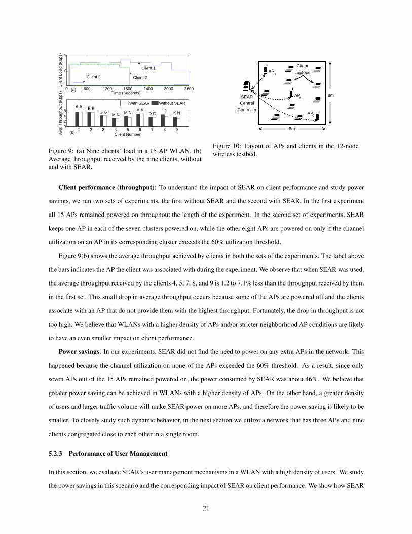
Figure 9: (a) Nine clients’ load in a 15 AP WLAN. (b)
Average throughput received by the nine clients, without
and with SEAR.
AP
AP
AP
A
B
C
SEARCentral
Controller
8m
8m
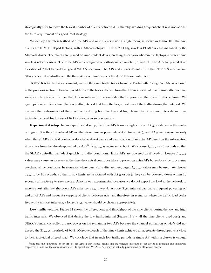
ClientLaptops
Figure 10: Layout of APs and clients in the 12-node
wireless testbed.
Client performance (throughput): To understand the impact of SEAR on client performance and study power
savings, we run two sets of experiments, the first without SEAR and the second with SEAR. In the first experiment
all 15 APs remained powered on throughout the length of the experiment. In the second set of experiments, SEAR
keeps one AP in each of the seven clusters powered on, while the other eight APs are powered on only if the channel
utilization on an AP in its corresponding cluster exceeds the 60% utilization threshold.
Figure 9(b) shows the average throughput achieved by clients in both the sets of the experiments. The label above
the bars indicates the AP the client was associated with during the experiment. We observe that when SEAR was used,
the average throughput received by the clients 4, 5, 7, 8, and 9 is 1.2 to 7.1% less than the throughput received by them
in the first set. This small drop in average throughput occurs because some of the APs are powered off and the clients
associate with an AP that do not provide them with the highest throughput. Fortunately, the drop in throughput is not
too high. We believe that WLANs with a higher density of APs and/or stricter neighborhood AP conditions are likely
to have an even smaller impact on client performance.
Power savings: In our experiments, SEAR did not find the need to power on any extra APs in the network. This
happened because the channel utilization on none of the APs exceeded the 60% threshold. As a result, since only
seven APs out of the 15 APs remained powered on, the power consumed by SEAR was about 46%. We believe that
greater power saving can be achieved in WLANs with a higher density of APs. On the other hand, a greater density
of users and larger traffic volume will make SEAR power on more APs, and therefore the power saving is likely to be
smaller. To closely study such dynamic behavior, in the next section we utilize a network that has three APs and nine
clients congregated close to each other in a single room.
5.2.3 Performance of User Management
In this section, we evaluate SEAR’s user management mechanisms in a WLAN with a high density of users. We study
the power savings in this scenario and the corresponding impact of SEAR on client performance. We show how SEAR
21
strategically tries to move the fewest number of clients between APs, thereby avoiding frequent client re-associations:
the third requirement of a good RoD strategy.
We deploy a wireless testbed of three APs and nine clients inside a single room, as shown in Figure 10. The nine
clients are IBM Thinkpad laptops, with a Atheros-chipset IEEE 802.11 b/g wireless PCMCIA card managed by the
MadWifi driver. The clients are placed on nine student desks, creating a scenario wherein the laptops represent nine
wireless network users. The three APs are configured on orthogonal channels 1, 6, and 11. The APs are placed at an
elevation of 7 feet to model a typical WLAN scenario. The APs and clients do not utilize the RTS/CTS mechanism.
SEAR’s central controller and the three APs communicate via the APs’ Ethernet interface.
Traffic traces: In this experiment, we use the same traffic traces from the Dartmouth College WLAN as we used
in the previous section. However, in addition to the traces derived from the 1 hour interval of maximum traffic volume,
we also utilize traces from another 1 hour interval of the same day that experienced the lowest traffic volume. We
again pick nine clients from the low traffic interval that have the largest volume of the traffic during that interval. We
evaluate the performance of the nine clients during both the low and high 1-hour traffic volume intervals and thus
motivate the need for the use of RoD strategies in such scenarios.
Experimental setup: In our experimental setup, the three APs form a single cluster. APA, as shown in the center
of Figure 10, is the cluster-head AP and therefore remains powered on at all times. APB and APC are powered on only
when the SEAR’s central controller decides to divert users and user load on to an extra AP based on the information
it receives from the already-powered on APs14. Tthresh is again set to 60%. We choose Ireconf as 5 seconds so that
the SEAR controller can adapt quickly to traffic conditions. Extra APs are powered on if needed. Longer Ireconf
values may cause an increase in the time the central controller takes to power on extra APs but reduces the processing
overhead at the controller. In scenarios where bursts of traffic are rare, larger Ireconf values may be used. We choose
Tidle to be 10 seconds, so that if no clients are associated with APB or APC they can be powered down within 10
seconds of inactivity to save energy. Also, in our experimental scenarios we do not expect the load in the network to
increase just after we shutdown APs after the Tidle interval. A short Tidle interval can cause frequent powering on
and off of APs and frequent swapping of clients between APs, and therefore, in scenarios where the traffic load peaks
frequently in short intervals, a longer Tidle value should be chosen appropriately.
Low traffic volume: Figure 11 shows the offered load and throughput of the nine clients during the low and high
traffic intervals. We observed that during the low traffic interval (Figure 11(a)), all the nine clients used APA and
SEAR’s central controller did not power on the remaining two APs because the channel utilization on APA did not
exceed the Tthresh threshold of 60%. Moreover, each of the nine clients achieved an aggregate throughput very close
to their individual offered load. We conclude that in such low traffic periods, a single AP within a cluster is enough
14Note that the “powering on or off” of the APs in our testbed means that the wireless interface of the device is activated and shutdown,
respectively - and not the entire device itself. In operational WLANs, APs may be actually powered on or off to save energy.
22
1 2 3 4 5 6 7 8 90
50
100
Meg
aByt
es
1 2 3 4 5 6 7 8 9
50010001500200025003000
Client Number
Meg
aByt
es
Offered Load
Client Throughput
Client Throughput with Load Diversion
(b)
(a)
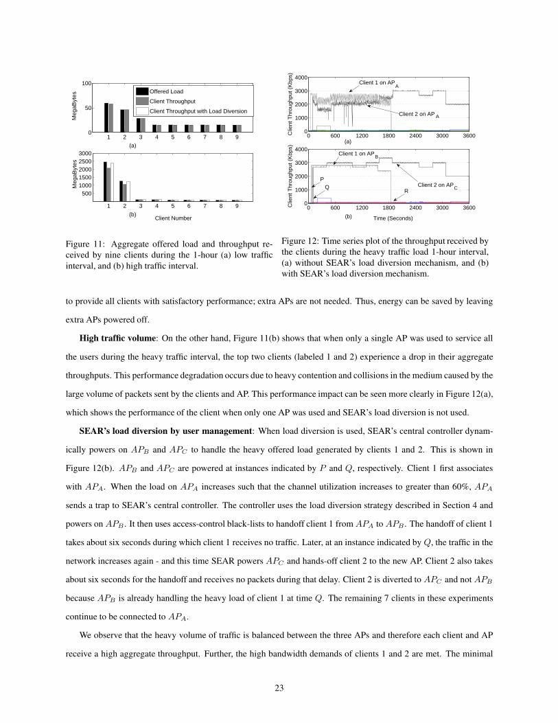
Figure 11: Aggregate offered load and throughput re-
ceived by nine clients during the 1-hour (a) low traffic
interval, and (b) high traffic interval.
0 600 1200 1800 2400 3000 36000
1000
2000
3000
4000
Clie
nt T
hrou
ghpu
t (K
bps)
0 600 1200 1800 2400 3000 36000
1000
2000
3000
4000
Time (Seconds)
Clie
nt T
hrou
ghpu
t (K
bps)
Client 1 on AP
Client 2 on AP
Client 2 on AP
Client 1 on AP
PQ
R
(a)
(b)
A
A
B
C
Figure 12: Time series plot of the throughput received by
the clients during the heavy traffic load 1-hour interval,
(a) without SEAR’s load diversion mechanism, and (b)
with SEAR’s load diversion mechanism.
to provide all clients with satisfactory performance; extra APs are not needed. Thus, energy can be saved by leaving
extra APs powered off.
High traffic volume: On the other hand, Figure 11(b) shows that when only a single AP was used to service all
the users during the heavy traffic interval, the top two clients (labeled 1 and 2) experience a drop in their aggregate
throughputs. This performance degradation occurs due to heavy contention and collisions in the medium caused by the
large volume of packets sent by the clients and AP. This performance impact can be seen more clearly in Figure 12(a),
which shows the performance of the client when only one AP was used and SEAR’s load diversion is not used.
SEAR’s load diversion by user management: When load diversion is used, SEAR’s central controller dynam-
ically powers on APB and APC to handle the heavy offered load generated by clients 1 and 2. This is shown in
Figure 12(b). APB and APC are powered at instances indicated by P and Q, respectively. Client 1 first associates
with APA. When the load on APA increases such that the channel utilization increases to greater than 60%, APA
sends a trap to SEAR’s central controller. The controller uses the load diversion strategy described in Section 4 and
powers on APB . It then uses access-control black-lists to handoff client 1 from APA to APB . The handoff of client 1
takes about six seconds during which client 1 receives no traffic. Later, at an instance indicated by Q, the traffic in the
network increases again - and this time SEAR powers APC and hands-off client 2 to the new AP. Client 2 also takes
about six seconds for the handoff and receives no packets during that delay. Client 2 is diverted to APC and not APB
because APB is already handling the heavy load of client 1 at time Q. The remaining 7 clients in these experiments
continue to be connected to APA.
We observe that the heavy volume of traffic is balanced between the three APs and therefore each client and AP
receive a high aggregate throughput. Further, the high bandwidth demands of clients 1 and 2 are met. The minimal
23
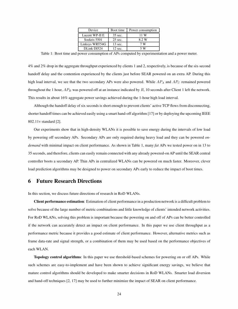
Device Boot time Power consumption
Lucent WP-II E 35 sec. 11 W
Soekris 5501 25 sec. 8.2 W
Linksys WRT54G 13 sec. 7 W
DLink DI524 12 sec. 5 W
Table 1: Boot time and power consumption of APs computed by experimentation and a power meter.
4% and 2% drop in the aggregate throughput experienced by clients 1 and 2, respectively, is because of the six-second
handoff delay and the contention experienced by the clients just before SEAR powered on an extra AP. During this
high load interval, we see that the two secondary APs were also powered. While APA and APC remained powered
throughout the 1 hour, APB was powered off at an instance indicated by R, 10 seconds after Client 1 left the network.
This results in about 16% aggregate power savings achieved during the 1-hour high load interval.
Although the handoff delay of six seconds is short enough to prevent clients’ active TCP flows from disconnecting,
shorter handoff times can be achieved easily using a smart hand-off algorithm [17] or by deploying the upcoming IEEE
802.11v standard [2].
Our experiments show that in high-density WLANs it is possible to save energy during the intervals of low load
by powering off secondary APs. Secondary APs are only required during heavy load and they can be powered on-
demand with minimal impact on client performance. As shown in Table 1, many fat APs we tested power on in 13 to
35 seconds, and therefore, clients can easily remain connected with any already powered-on AP until the SEAR central
controller boots a secondary AP. Thin APs in centralized WLANs can be powered on much faster. Moreover, clever
load prediction algorithms may be designed to power on secondary APs early to reduce the impact of boot times.
6 Future Research Directions
In this section, we discuss future directions of research in RoD WLANs.
Client performance estimation: Estimation of client performance in a production network is a difficult problem to
solve because of the large number of metric combinations and little knowledge of clients’ intended network activities.
For RoD WLANs, solving this problem is important because the powering on and off of APs can be better controlled
if the network can accurately detect an impact on client performance. In this paper we use client throughput as a
performance metric because it provides a good estimate of client performance. However, alternative metrics such as
frame data-rate and signal strength, or a combination of them may be used based on the performance objectives of
each WLAN.
Topology control algorithms: In this paper we use threshold-based schemes for powering on or off APs. While
such schemes are easy-to-implement and have been shown to achieve significant energy savings, we believe that
mature control algorithms should be developed to make smarter decisions in RoD WLANs. Smarter load diversion
and hand-off techniques [2, 17] may be used to further minimize the impact of SEAR on client performance.
24
Client participation: We envision future WLAN scenarios wherein clients actively participate in conserving
energy by informing the WLAN about when they need resources, how many, and for how long. In such scenarios,
WLANs can generate schedules and power on APs only during predetermined intervals of time.
Infrastructure support: Extra energy savings can be achieved if power-hungry switches and controllers in the
WLAN can also be powered off during intervals of low demand. The powering off of switches and controllers may
require WLAN managers to strategically re-wire APs to different switches so that the powering off of APs and the
switches can be coordinated efficiently [10].
Hardware modifications: Better hardware-based power standby modes can be used to save more energy and even
further minimize the impact on client performance. Strategies such as SEAR can utilize specialized standby modes on
APs for faster powering on of the APs.
7 Conclusions
This paper proposes the adoption of resource on-demand (RoD) WLAN strategies that can efficiently reduce energy
consumption of a WLAN without adversely impacting the performance of clients in the network. We stress that
energy-efficient mechanisms for large-scale and high-density WLANs should be designed and developed today - to
save energy in future WLANs and thus avoid the escalation of energy wastage.
We have proposed a practical RoD strategy, called SEAR. We have demonstrated that SEAR can be easily imple-
mented using current devices, and the on-demand powering of APs is a feasible strategy that does not adversely impact
end-user performance. We have also discussed several interesting problems as future research directions towards the
wide-spread deployment of RoD WLANs. Our next step is to evaluate the performance of SEAR in large-scale
WLANs.
The most important message of this paper is that the energy wasted in large-scale and high-density WLANs is
a new and serious concern. This paper makes the first attempt at designing strategies to reduce energy wastage in
WLANs. However, additional work is still needed to avoid the escalation of energy wastage in the future.
References
[1] Dartmouth College WLAN. http://crawdad.cs.dartmouth.edu.
[2] IEEE 802.11v: Wireless Network Management. http://grouper.ieee.org/groups/802/11/Reports/tgv update.htm.
[3] IETF CAPWAP WG: http://www.ietf.org/html.charters/capwap-charter.html.
[4] Aruba Selected by Microsoft For Next Generation Wireless LAN. http://www.arubanetworks.com/news/release/2005/06/13, 2005.
[5] Forrester Research. http://www.forrester.com, 2006.
[6] Y. Bejerano. Efficient Integration of Multi-hop Wireless and Wired Networks with QoS constraints. In ACM Mobicom, Atlanta, GA, September 2002.
25
[7] J. S. Chase, D. C. Anderson, P. N. Thakar, A. Vahdat, and R. P. Doyle. Managing Energy and Server Resources in Hosting Centres. In SOSP, Banff, Canada,October 2001.
[8] K. J. Christensen, C. Gunaratne, B. Nordman, and A. D. George. The Next Frontier for Communications Networks: Power Management. Elsevier Computer
Communications, 27:1758–1770, June 2004.
[9] M. Gupta and S. Singh. Greening of the Internet. In ACM SIGCOMM, Karlsruhe, Germany, August 2003.
[10] A. P. Jardosh, G. Iannaccone, K. Papagiannaki, and B. Vinnakota. Towards an Energy-Star WLAN Infrastructure. In HotMobile, Tucson, AZ, February 2007.
[11] A. P. Jardosh, K. N. Ramachandran, K. C. Almeroth, and E. M. Belding. Understanding Link-Layer Behavior in Highly Congested IEEE 802.11b WirelessNetworks. In Proceedings of ACM SIGCOMM Workshop E-WIND, Philadelphia, PA, August 2005.
[12] A. P. Jardosh, K. N. Ramchandran, K. C. Almeroth, and E. M. Belding. Understanding Congestion in IEEE 802.11b Wireless Networks. In Proceedings of
USENIX IMC, Berkeley, CA, October 2005.
[13] D. Kotz, T. Henderson, and I. Abyzov. CRAWDAD trace set dartmouth/campus/snmp (v. 2004-11-09). Downloaded fromhttp://crawdad.cs.dartmouth.edu/dartmouth/campus/snmp, Nov. 2004.
[14] A. Meka and A. K. Singh. Distributed Spatial Clustering in Sensor Networks. In EDBT, Munich, Germany, March 2006.
[15] N. Mishra, K. Chebrolu, B. Raman, and A. Pathak. Wake-on-WLAN. In ACM WWW, Edinburgh, UK, May 2006.
[16] E. Pinheiro, R. Bianchini, and C. Dubnicki. Exploiting Redundancy to Conserve Energy in Storage Systems. In Sigmetrics, Saint Malo, France, June 2006.
[17] I. Ramani and S. Savage. SyncScan: Practical Fast Handoff for 802.11 Infrastructure Networks. In Proceedings of IEEE Infocom, Miami, FL, March 2005.
[18] C. Reis, R. Mahajan, M. Rodrig, D. Wetherall, and J. Zahorjan. Measurement-Based Models of Delivery and Interference in Static Wireless Networks. In ACM
Sigcomm, Pisa, Italy, September 2006.
[19] M. Rodrig, C. Reis, R. Mahajan, D. Wetherall, and J. Zahorjan. Measurement-based Characterization of 802.11 in a Hotspot Setting. In Proceedings of EWIND,Philadelphia, PA, August 2005.
26