Embed Size (px)
Citation preview
Computing Society
14th INFORMS Computing Society ConferenceRichmond, Virginia, January 11–13, 2015pp. 134–148
http://dx.doi.org/10.1287/ics.2015.0010Creative Commons License
This work is licensed under aCreative Commons Attribution 3.0 License
Green Vehicle Routing Problem withTime-Varying Traffic Congestion
Yiyong Xiao and Abdullah KonakSchool of Reliability and System Engineering, Beihang University, Beijing, China,[email protected]
Information Sciences and Technology, Penn State Berks, Reading, PA 19610, [email protected]
Abstract We present a linear mixed integer programming model for the time-dependent hetero-geneous green vehicle routing and scheduling problem (GVRSP) with the objective ofminimizing total carbon dioxide emissions and weighted tardiness. Instead of discretetime intervals, the proposed model takes the traveled distances of arcs in differenttime periods as decision variables to determine the travel schedules of vehicles. Wepropose an exact dynamic programming method to calculate the optimal discretedeparture/arriving time for the GVRSP. The dynamic programming method signifi-cantly reduces the computational complexity of the GVRSP when applying existingheuristic algorithms to solve large-sized problems. A genetic algorithm with dynamicprogramming (GA-DP) is developed to solve the formulated problem. Computationalexperiments are carried out to study the efficiency of the proposed hybrid solutionapproach with promising results.
Keywords CO2 emissions, vehicle routing, mixed integer programming, dynamic programming,genetics algorithms, hybrid optimization
1. Introduction
It is well recognized that carbon dioxide (CO2) is the major contributor of the global warm-ing effect of the Earth during the past decades. Since it was first measured in 1958, theconcentration of CO2 in Earth’s atmosphere has been continuously increasing [27]. Accord-ing to the International Energy Agency (IEA), the transportation sector, after electricitygeneration and heating, was the second-largest contributor of CO2 emissions, representing22% of the global CO2 emissions in 2010, and almost three-quarters of the emissions fromtransportation were due to road transportation [1]. Traffic congestion, which results in lowspeeds with fluctuations on roads, often companied with frequent acceleration and decel-eration, had greatly contributed to CO2 emissions [2, 15]. Therefore, reducing fossil fuelconsumption and CO2 emissions due to road transportation through optimizing transporta-tion operations is important for controlling the global warming. The objective of this paper isto develop new mathematical models and optimization methods for reducing CO2 emissionsin the context of the Vehicle Routing Problem (VRP) with traffic congestion considerations.
The Vehicle Routing Problem (VRP) has been a classic and important optimization prob-lem in road transportation applications since its introduction by Dantzig and Ramser [6]. Ingeneral, the VRP is concerned with determining the optimal routes used by a fleet of vehi-cles, stationed at one or multiple depots, with the objective of fulfilling customers’ demandsat minimum cost. Various versions of the VRP have been developed for different applica-tions in the past half century, such as pickup and delivery VRP, capacitated VRP, VRPwith multiple depots, VRP with time windows, split delivery VRP, time-dependent VRP,
134
Xiao and Konak: Green Vehicle Routing ProblemICS-2015—Richmond, pp. 134–148, c© 2015 INFORMS 135
etc. Surveys on various VRP formulations and algorithms can be found in Laporte et al.[23], Toth and Vigo [29], Golden et al. [18], and Eksioglu et al. [11].
In the recent decade, Green VRP [24, 10], which is characterized by the objective of bal-ancing environmental and operational costs, has attracted the attention of researchers inthe VRP literature. Ericsson et al. [13] identified the impact of traffic disturbances on fuelconsumption and proposed a model for estimating the potential reduction in fuel consump-tion through route optimization. Kara et al. [20] proposed a cost function in terms of energyconsumption for the VRP and named it as the Energy Minimizing VRP (EMVRP), whichminimizes the total energy consumption in the route (instead of the total distance) to reducefuel consumption and CO2 emissions. Reducing CO2 emissions also helps to save fuel costbecause CO2 emissions are usually proportional to the amount of fuel consumption [26].Tavares et al. [28] took into account the effect of both road inclination and vehicle load onfuel consumption in waste collection operations. Kuo [21] proposed a mathematical model tocalculate the total fuel consumption for the time-dependent VRP, considering both loadingweight and the “non-passing” property. Figliozzi [14] proposed a partial-emissions minimiz-ing VRP (EVRP) model to optimize the departure times of vehicles on the routes foundby a time-dependent VRP algorithm. Xiao et al. [30] incorporated the fuel consumptionrate resulted from a vehicle’s load (which is decreasing/increasing along the tour) into theVRP and proposed a mathematical model considering fuel consumption rate. Erdogan andMiller-Hooks [12] presented a Green VRP and developed solution techniques to aid organi-zations with alternative fuel vehicles working in a long driving range in conjunction with alimited refueling infrastructure. Kwon et al. [22] developed a heterogeneous fixed fleet VRPmodel that considers the CO2 emissions trade cost in the objective function. Gaur et al. [16]studied the cumulative VRP where vehicles have finite capacity and an arbitrary numberof depot offloads are allowed and proposed an approximation algorithm to minimize fuelconsumption. Demir et al. [9] proposed an adaptive large neighborhood search algorithm(ALNS) to minimize the fuel consumption and the driving time with Pareto optimality.
Traffic congestion usually causes road conditions to be time-dependent, and the VRPunder this case is called the time-dependent VRP (TDVRP) [25, 4, 14]. Compared with thedistance-based VRP, the TDVRP considers the departure time at each node as a decisionvariable. Because the total travel time depends on node departure times as well as routes, theTDVRP is usually studied with an alternative objective such as minimizing the total traveltime, fuel consumption, or CO2 emissions [14, 21]. The TDVRP is a much more challengingproblem to solve than the traditional VRP because the solution space is exponentiallyincreased by the introduction of node departure time decisions which are often modeled asinteger variables.
Recently, Bektas and Laporte [3] presented the pollution routing problem (PRP) byextending the classical VRP with time windows (VRPTW) as well as with a more compre-hensive objective function including fuel, emission, and driver costs. In the PRP, the vehicleload and speed on each route segment are considered as decision variables. Demir et al. [8]developed a two-stage heuristic algorithm to solve the PRP of large-size instances with up to200 nodes. In this two-stage approach, a large neighborhood search (LNS) heuristic is usedto solve traditional VRPTW in the first stage, and the optimal speed for each arc of theroute is determined optimally in the second state. Franceschetti et al. [15] extended the PRPto Time-Dependent PRP (TDPRP) by considering traffic congestion. In their approach, theplanning horizon is divided into two periods: (1) the initial period of traffic congestion witha lower and constant speed and (2) the period with a speed range where the travel timelinearly depends on the departure time.
In this paper, we consider a general case of the time-dependency for vehicle routing andmultiple time periods for vehicle scheduling, with the objective of minimizing the total CO2
emissions and tardiness. A tardiness objective is considered for the first time in the contextof the green VRP. Tardiness objectives are frequently used in the scheduling literature to
Xiao and Konak: Green Vehicle Routing Problem136 ICS-2015—Richmond, pp. 134–148, c© 2015 INFORMS
model the timeliness of a service where it is impossible to satisfy all customer orders on timedue to capacity limits. In such cases, the time that a customer is serviced late is penalizedby a tardiness penalty coefficient representing the loss of customer goodwill. The magnitudeof tardiness penalty represents the relative importance of customers. In this paper, roads areassumed to have various patterns of traffic congestion, and the scheduling horizon may havemultiple periods and arbitrary departing times. The problem is formulated to optimize green-house gas emissions through both arcs routing and time scheduling. Therefore, it is referredto as the Green Vehicle Routing and Scheduling Problem (GVRSP). The proposed GVRSPformulation contributes to the existing body of research on the green time-dependent VRPin several ways. Compared to most green time-dependent VRP where only node departuretimes are considered as decision variables, in the GVRSP herein we consider: (i) multipletime periods for traveling arcs, (ii) the total traveled distances of arcs in each time period,and (iii) the optimal departure time and arrival times for arcs in each time period. In otherwords, we present an alternative formulation for modeling time-dependency using the totaltraveled distance of an arc in each period as the primary decision variable instead of thedeparture time of an arc. Thereby, an arc can be traveled in multiple time periods. Theproposed GVRSP formulation is linear and can be solved optimally by most existing MIPsolvers for small-sized problems. In this sense, the proposed formulation is a more generalmodel for combined routing and scheduling decisions in the context of the GVRSP. In addi-tion to a more flexible way of modeling time-dependency, we also consider multiple vehicletypes in the proposed formulation. The existing GVRSP models in the literature generallyassume a single vehicle type. However, CO2 emissions highly depend on the vehicle type.
To solve the GVRSP efficiently, we propose a hybrid approach of a genetic algorithm(GA) and dynamic programming for the two groups of the decision variables, routing andscheduling. The GA searches for the routing and vehicle selection decisions, and dynamicprogramming is used to optimize the scheduling decision of the selected vehicles and routes.Therefore, the proposed hybrid approach is called the GA-DP. We demonstrate that theproposed approach can solve large-sized problem instances.
2. Problem Description and Formulation
The GVRSP herein is described as follows. A set of heterogeneous vehicles is going to visitn customers randomly located in a region, starting from and ending at a depot. Let set Hbe the set of vehicles and q denote the cardinality of set H. Each vehicle h has a maximumcapacity of Ch and a maximum travel range of Lh depending on its type. The problem isdefined on a complete directed network G(N,A) where N = {0,1, ..., n} is the node set, andA= {(i, j) : i 6= j, i, j ∈N} is the set of arcs. Node 0 represents the depot, and N ′ =N \ {0}is the set of customers. Each arc (i, j) represents the path between nodes i and j, and thedistance of arc (i, j) is denoted by Dij . Each customer i has a demand Ri and requires aservice time gi within the time-window [0,Ei] where Ei is the due-time of customer i suchthat a late visit will result in a tardiness penalty ωi per unit time tardy.
The time horizon is divided arbitrarily into m time periods such that the traffic speeds onroads are assumed to be fixed within a time period but may be different between two timeperiods. Let set K represent the set of time periods, and each period k ∈K is identified byits beginning time bk and ending time ek. The travel speed of vehicles on arc (i, j) in timeperiod k (vijk) is also assumed to be known, and the CO2 emissions rate (Lb/mile) of vehicleh when traveling on arc (i, j) in time period k (cijkh) can be calculated using emissionsmodels from the literature. Note that all road and vehicle conditions such as speed, slope,traffic congestion, vehicle weight, can be factored into the calculation of cijkh.
The problem involves four decisions for each vehicle as follows: (1) whether to use a vehicleor not, (2) the route to visit customers if a vehicle is used, (3) the departure and arrival timeschedule for each node in the tour, and (4) the distances to be traveled on each arc in each
Xiao and Konak: Green Vehicle Routing ProblemICS-2015—Richmond, pp. 134–148, c© 2015 INFORMS 137
time period. The objective of the problem is to minimize the total amount of CO2 emissions
and tardiness penalties. Comparing to the traditional TD-VRP, the GVRSP formulated in
this paper is more general as idle time can be scheduled anywhere in the tour to avoid traffic
congestions. The decision variables of the model are as follows:
Xij binary variable indicating whether arc (i, j) is traveled (Xij = 1) or not (Xij = 0)yijh binary variable indicating whether arc (i, j) is traveled by vehicle h (in any period)
(yijh = 1) or not (yijh = 0)xijkh binary variable indicating whether arc (i, j) is traveled by vehicle h in period k
(xijkh = 1) or not (xijkh = 0)dijkh continuous variable indicating the traveled distance of arc (i, j) in time period k by
vehicle hτijkh continuous variable indicating the travel time of vehicle h on arc (i, j) in time period k
li continuous variable indicating the departure time from node i (the earliest departuretime for i= 0)
ai continuous variable indicating the arrival time at node i (the latest arrival time fori= 0)
Oi tardiness of node i
Problem GVRSP:
Minimize F =
q∑h=1
n∑i=0
n∑j=0:i 6=j
m∑k=1
dijkh · cijkh +
n∑i=1
ωi ·Oi
Subject to:n∑
j=0
Xij = 1 ∀i∈N ′ (1)
n∑i=0
Xij = 1 ∀j ∈N ′ (2)
Xij =
q∑h=1
yijh ∀(i, j)∈A (3)
yijh ≥ xijkh ∀(i, j)∈A,k ∈K,h∈H (4)
yijh ≤m∑
k=1
xijkh ∀(i, j)∈A,h∈H (5)
n∑i=0:i 6=j
yijh =
n∑i=0:i 6=j
yjih ∀h∈H,j ∈N (6)
n∑j=1
y0jh ≤ 1 ∀h∈H (7)
dijkh ≤Dij ·xijkh ∀(i, j)∈A,k ∈K,h∈H (8)m∑
k=1
q∑h=1
dijkh =Xij ·Dij ∀(i, j)∈A (9)
τijkh = 60 · dijkh/vijk ∀(i, j)∈A,k ∈K,h∈H (10)∑(i,j)∈A
τijkh ≤ ek − bk ∀k ∈K,h∈H (11)
li ≤ ek − τijkh+em · (1−xijkh) ∀(i, j)∈A,k ∈K,h∈H (12)
Xiao and Konak: Green Vehicle Routing Problem138 ICS-2015—Richmond, pp. 134–148, c© 2015 INFORMS
aj ≥ bk + τijkh− em · (1−xijkh) ∀(i, j)∈A,k ∈K,h∈H (13)
aj ≥ li +
m∑k=1
q∑h=1
τijkh− em · (1−Xij) ∀(i, j)∈A (14)
ai + gi ≤ li ∀i∈N ′ (15)
a0 ≤ em (16)n∑
j=1
n∑i=0
Rj · yijh ≤Ch ∀h (17)
∑(i,j)∈A
Dij · yijh ≤Oh ∀h (18)
Oi ≥ ai−Ei ∀i∈N ′ (19)
dijkh, τijkh ≥ 0
li, ai,Oi ≥ 0
Xij , yijh, xijkh ∈ {0,1}
In Problem GVRSP, Constraints (1) and (2) ensure that each customer is visited only once.Constraint (3) states that a selected arc can be traveled only by one vehicle. Constraints(4) and (5) force variable yijh to be consistent with variable xijkh. Constraint (6) is thenode balance constraint for each vehicle, ensuring that each vehicle enters and departs fromeach node in equal number of times. Constraint (7) indicates that each vehicle leaves thedepot at most only one time (i.e., a vehicle cannot be used again after it returns back to thedepot). Constraints (8) ensures that dijkh becomes zero if xijkh = 0. On the other hand, ifxijkh = 1, the value of dijkh is bounded to Dij by Constraints (8). Constraint (9) guaranteesthat the total distance of arc (i, j) must be traveled once the arc is selected. Constraint(10) calculates the travel time of dijkh (the travel time is measured in seconds, and thetravel speed unit is miles-per-hour). Note that Constraint (10) is linear because vijk is acalculated parameter. Thereby, it is possible to express the non-linear relationship betweenCO2 emissions and the travel-speed as linear constraints without requiring auxiliary binaryvariables for linearization. Constraint (11) ensures that the total travel time of each vehiclein each time period is less than the duration of the time period. Constraint (12) ensuresthat if arc (i, j) is traveled in time period k, the departure time of node i must be beforethe end time of time period k subtracted by the travel time of arc (i, j) in time period k.Similarly, Constraint (13) states that the arrival time of node j must be greater than orequal to the start time of time period k plus the travel time of arc (i, j) in time period k.These two constraints are only active for xijkh = 1. Note that for xijkh=0, Constraints (12)and (13) still hold because em is a large enough number that guarantees the validity of theinequities. Constraint (14) is a disjunctive constraint to calculate the earliest arrival timeat node j. Note that Constraint (14) is only active for the arcs that are selected in a tour(i.e., Xij = 1). Constraint (15) ensures that the vehicle’s departure time must be after itsarrival time plus the service time on each customer node i. Constraints (14) and (15) alsoeliminate any sub-tours among customers. Constraint (16) requires that the return time tothe depot must not exceed the end time of the last period. Constraints (17) and (18) are forvehicles’ capacity and travel length limits, respectively. Constraint (19) is a linear expressionfor calculating the tardiness value.
It should be noted that although there are 10 different types of decision variables inProblem GVRSP, most of them are tightly bounded (directly or indirectly) to independentdecision dijkh variables. In addition, all mathematical expressions in the model are linear.Therefore, it is possible to optimally solve Problem GVRSP using existing off-the-shelfsolvers. In the experimental section, we used AMPL/CPLEX (version 12.4.0.1) to optimallysolve Problem GVRSP for small-sized problem instances.
Xiao and Konak: Green Vehicle Routing ProblemICS-2015—Richmond, pp. 134–148, c© 2015 INFORMS 139
3. Description of the Hybrid Genetic Algorithm and DynamicProgramming
Problem GVRP can be optimally solved only for small-sized problems. In this section, wepropose an exact dynamic programming (DP) procedure to calculate the optimal depar-ture and arrival time of each vehicle at each node for a given set of tours. Since the DPmethod has polynomial computational complexity, the complexity of the GVRSP can bereduced significantly by dividing the problem in two parts, routing and scheduling. Oneof the challenges of applying meta-heuristic algorithms to solve the GVRSP is devisingan encoding schema to effectively represent the problem’s binary and continuous decisionvariables. Note that the continuous schedule decision variables depend on the binary routedecision variables. Therefore, when the routes of a solution are perturbed by local or globalsearch operators, the schedule decision variables must also be modified accordingly. Oth-erwise, the structure of the solution will be destroyed. This makes the GVRSP difficult tosolve by meta-heuristics. If the problem is solved in two phases as routing and scheduling asproposed in this paper, the solution encoding is significantly simplified because the scheduledecision variables can be determined by the DP procedure for a given set of routes.
3.1. Solution Encoding
In the GA, the routes of a solution are encoded as an ordered-string vector. We use Sh ={shp : p= 1,2, ..., nh−1} to represent the sequence of the customer nodes visited by vehicle h,starting from and returning back to depot 0, where
nh the number of arcs traveled by vehicle h (e.g., if a vehicle h visits only onecustomer and returns back to the depot, then nh = 2),
shp the index of the customer node at the pth position of vehicle h’s tour,p node index of a vehicle’s tour.
For a problem with a maximum of q vehicles, S is constructed as S = {0+S1 +0+S2 +0+...+0+Sq +0} with zeroes between the route strings representing the start of a new tour. Forexample in a problem with three vehicles and five customers, if a solution has S1 = {3,5,2},S2 = {}, S3 = {1,4}, then the solution in the GA is represented as S = {0,3,5,2,0,0,1,4,0}.
3.2. Dynamic Programming
Let r denote the index of arcs traveled by a vehicle for r= 1,2, ..., nh (e.g., (sh0 , sh1 ) is the first
arc traveled by vehicle h). For each vehicle h, we use integer variables lhr and ahr to representthe departure time (vehicle h starts traveling the rth arc of Sh) and the arrival time (vehicleh finishes traveling the rth arc of Sh) of arc r, respectively. Note that in Problem GVRSP,variables li and ai are defined in the continuous domain, but they are discretized as integervariables for DP. If the time unit is small enough, the difference between the schedulesbased on continuous and discrete times will be very small and can be ignored in real-lifeapplications.
In this section, we introduce a DP procedure to determine the optimal departure timelhr and arrival time ahr for a given Sh. The planning horizon is divided into T integer unitsof time, t = 0,1,2, ..., T , which represent the discretized time points when the vehicle candepart from a node and arrive at the next one according to route Sh. For a given Sh, theDP model has nh stages. In stage r, the state of vehicle h is defined by t and t′, representingthe departure and arrival times of the rth arc such that t, t′ ∈ [0, T ] and t≤ t′. For vehicle h,we use the following notations in the DP model.
Xiao and Konak: Green Vehicle Routing Problem140 ICS-2015—Richmond, pp. 134–148, c© 2015 INFORMS
zhrtt′ the optimal objective function value caused by traveling the rth arc between times tand t′.
fhrt the optimal objective function value for starting at time t and traveling the rth,(r+ 1)th,..., (nh)th arcs.
ηhrt the corresponding arrival time of traveling the rth arc for each of fhrt.Fh the optimal objective function value of vehicle h.j(r) the index of the head node of the rth arc.vrk the traffic speed of the rth arc in time period k.crkh CO2 emission rate of vehicle h when traveling on the rth arc in time period k.µktt′ the length of the time interval overlapped between time period k and interval [t, t′].drkh the distance travelled on the rth arc in time period k by vehicle h.
The zhrtt′ can be optimally determined by solving the following trivial linear programmingproblem.
Minimize zhrtt′ =∑k∈K
crkh · drkh + max{0, ωj(r) · (t′−Ej(r))}
Subject to:
drkh ≤ vrk ·µktt′ ∀k ∈K (20)
Dr =∑k∈K
drkh (21)
drkh ≥ 0
The tardiness part of the objective function, i.e. max{0, ωj(r) · (t′−Ej(r))}, is a constantbased only on t′. The CO2 emissions part of the objective function can be optimally deter-mined by assigning the maximum possible value to variable drkh with the smallest valueof crkh until constraint Dr =
∑k∈K drkh is satisfied. If there is no feasible solution to the
problem because time interval [t, t′] is not long enough to cover distance Dr, then zhrtt′ =∞.After determining zhrtt′ , the recursive backward equation for the DP model is given asfollows:
fhrt =
{min{zhrtt′ : t′ = 0,1,2, ..., T} r= nh
min{zhrtt′ + fh(r+1)t′ : t′ = 0,1,2, ..., T} r= nh− 1, ...,2,1
(22)
By using equation (22), all values of fhrt and ηhrt can be deduced starting from r = nh to1 for each time point t= 0,1,2, ..., T . Thus, we can determine the optimal objective valuefor vehicle h as Fh = min{fh1t : t = 0,1,2, ..., T}, and the corresponding departure time lh1for the first arc. After that, the optimal ahr and lhr can be determined from r = 2 to nh.Using the same procedure, the optimal departure times and arriving times can be calculatedfor all used vehicles, and the total optimal objective value of all used vehicles is given asF =
∑qh=1F
h.The worst case computational complexity of the dynamic programming procedure is
O((nT )2). For each sub-tour h of a solution, the calculation of zhrtt′ is computationallyexpensive although it can be done in polynomial time. Fortunately, the calculation of zhrtt′can be omitted using a pre-calculated matrix Zh
ijtt′ -the optimal objective function value oftraveling arc (i, j) by vehicle h if the vehicle departs from node i at time t and arrives atnode j at time t′. In the actual implementation of the DP procedure, zhrtt′ is not calculatedfor each individual sub-tour of a candidate solution as it can be obtained by directly froma pre-calculated matrix Zh
ijtt′ . In Algorithm 1, the procedure for pre-calculating Zhijtt′ is
provided. Note that this procedure finds the optimum solution for the linear programmingmodel given above. The procedure always selects the period that leads to minimum CO2
emissions for the vehicle to travel. In Algorithm 1, Line 1 calculates the length of the time
Xiao and Konak: Green Vehicle Routing ProblemICS-2015—Richmond, pp. 134–148, c© 2015 INFORMS 141
interval that [t, t′] and [bk, ek] overlap for each time period k. Between Lines 3 and 17, vehicleh travels arc (i, j) on the time periods with minimum possible CO2 emissions. In Lines 18and 19, the tardiness penalty part of the objective function is calculated. A drawback of thisapproach is that matrix Zh
ijtt′ can be very large. Nonetheless, matrix Zhijtt′ is also a sparse
matrix which can be efficiently stored in the computer memory using sparse matrix storagetechniques. As shown in the computational experiment section, large-sized problems can besolved efficiently.
Algorithm 1 Calculation the optimal objective value for Zhijtt′
1: Set µktt′←max(0,min(ek, t′)−max(bk, t)) ∀k ∈K
2: obj← 0, dis←Dij
3: while dis > 0 do4: k∗← arg min
k∈K(cijkh : µktt′ > 0)
5: if k∗ does not exits then return −16: end if7: if dis > vijk∗ ·µk∗tt′/60 then8: dijk∗h← vijk∗ ·µk∗tt′/609: obj← obj+ cijk∗h · dijk∗h
10: µk∗tt′← 011: dis← dis− dijk∗h12: else13: dijk∗h← dis14: obj← obj+ cijk∗h · dis15: dis← 016: end if17: end while18: if t′ >Ej(r) then19: obj← obj+ωj(r) · (t′−Ej(r))20: end if21: Return obj
The following two properties on Zhijtt′ and fhrt can be used to further improve the compu-
tational efficiency of the DP procedure further.Property 1 Zh
ijt1t′, if exists, is a monotonically increasing function of t as follows:
Zhijt1t′ ≥Z
hijt2t′ ∀h, i, j, t
′ and t1 < t2 (23)
Property 2 For a tour Sh, fhrt1 , if exists, is a monotonically increasing function of thedeparture time t of arc r as follows:
fhrt1 ≤ fhrt2 ∀h, r and t1 < t2 (24)
Using the above two properties, for each arc r in Sh, the earliest arrival time t∗ (denotedas t∗1) that leads to optimal zhrtt∗ can be pre-calculated for each departure time t in [0, T ].In addition, the latest departure time (denoted as t∗2) that leads to optimal fhrt can be pre-determined in the previous calculation for arc r+ 1. Therefore, fhrt can be calculated moreefficiently using the following recursive backward equation:
fhrt =
{zhrtt∗1 if t∗1 ≤ t∗2 or r= nh
min(zhrtt′ + f(t+1)t′ : t∗2 ≤ t′ ≤ t∗1) if t∗1 > t
∗2 and r < nh
(25)
Xiao and Konak: Green Vehicle Routing Problem142 ICS-2015—Richmond, pp. 134–148, c© 2015 INFORMS
Thus, the calculation of fhrt can be either obtained directly from pre-calculated matrix (forthe cases t∗1 ≤ t∗2 or r = nh) or from the minimum zhrtt′ + fhr+1,t′ such that t′ is within[t∗2, t
∗1]. This approach further simplifies the computational complexity of the DP procedure.
Note that if t∗1 ≤ t∗2, then the vehicle can have an idle time of t∗2− t∗1 before starting to travelthe rth arc in Sh, which does not impact the objective function value. If fhrt cannot becomputed for t= 0 (i.e., the rth arc cannot be traveled before completing the route within[0, T ]), then the route is infeasible. For this case, in order to include infeasible solutions inthe evolution process of the GA, we set fhrt = β ·max{zhrtt′ : ∀t, t′}+ fh(r+1)t∗2
for the rth arc
and all arcs before it in Sh, where β is a dynamic penalty coefficient which is introduced inthe following section. In other words, the worst objective value of traveling the rth arc isused as a penalty term if it cannot be traversed completely.
3.3. Description of the Genetic Algorithm
3.3.1. Solution Initialization. We use a random construction heuristic to initialize thepopulation as follows: (1) initialize S with only q+ 1 zeros (vehicles), i.e., S = 0,0,0, ...,0,(2) find a customer i who has the least increase in the objective function value and insert itinto a position p in S, (3) repeat step 2 until all customers are inserted into S, (4) use Insertand Swap operators to randomly perturb the tour. After S is initialized, the DP procedureis called to calculate the schedule of the vehicles.
3.3.2. Genetic Operators. Three genetic operators, which are Insert, Swap, and Cross-over, are used in turn to reproduce new routes from the existing ones in the population. TheInsert operator relocates a randomly selected node to a randomly selected position in S.The Swap operator swaps the positions of two randomly selected nodes in S.
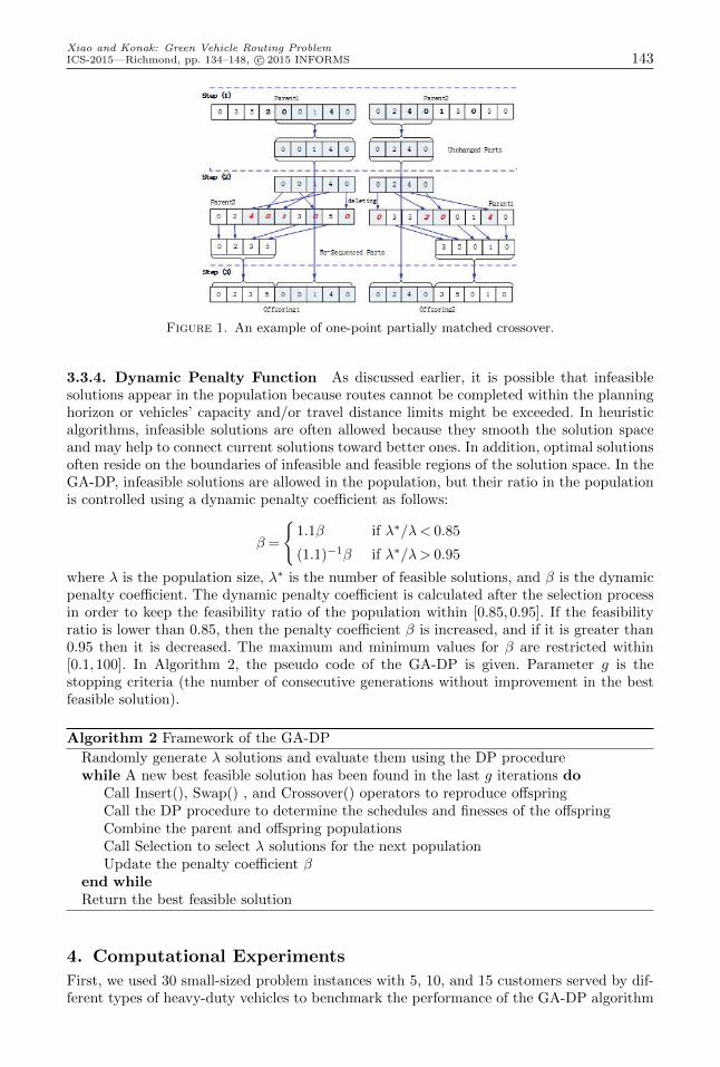
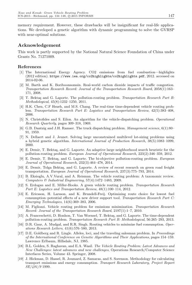
The Crossover operator is a one-point partially matched crossover [17], which recom-bines two randomly selected parents to produce two offspring. Each of the two offspringinherits an unchanged-part from one parent and a re-sequenced-part from the other par-ent as shown in Figure 1. The unchanged part is transferred from one parent to an off-spring exactly. The genes of the re-sequenced-part are transferred to the offspring afterrearranging them according to the sequence of the same genes in the other parent. Anexample of the crossover operator is given in Figure 1, where Parent 1={0,3,5,2,0,0,1,4,0}and Parent 2={0,2,4,0,1,3,0,5,0} are recombined at a point p to generate two offspring{0,2,3,4,0,0,1,4,0} and {0,2,4,0,3,5,0,1,0}. In the figure, the genes indicated by italictypefaces in Parent 1 and Parent 2 are the genes in one parent that have the same sequencein the other parent, and deleting them produces the re-sequenced part of the offspring.
The three operators are used in turn to reproduce a new population of solutions. Therefore,the size of the population expands to 5λ from λ after all operators are applied.
3.3.3. Fitness Calculation and Selection. The fitness of solution i is defined as follows:
Pi = exp
(− Fi−Fmin
Favg−Fmin
)where Fi is solution i’s objective function value calculated by the DP procedure, and Fmin
and Favg are respectively the minimum and average objective function values in the pop-ulation. Pi is the probability for solution i to stay in the population during the selectionprocedure. For a solution with the average objective function value, the fitness probabilityis exp(−1)≈ 0.37.
Selection is the procedure of reducing the size of the expanded population (due to repro-duction by mutation and crossover) to a fixed size by deleting individuals based on theirfitness probabilities. To maintain the diversity of the population, we use the clusteringmethod introduced by Dellaert and Jeunet [7] to group individuals with identical objectivevalues as one cluster and retain at most 10 individuals in the best cluster and only one indi-vidual in any other clusters. Therefore, an individual can be removed from the populationeither because it is not fit enough or because of the size of its cluster.
Xiao and Konak: Green Vehicle Routing ProblemICS-2015—Richmond, pp. 134–148, c© 2015 INFORMS 143
Figure 1. An example of one-point partially matched crossover.
3.3.4. Dynamic Penalty Function As discussed earlier, it is possible that infeasiblesolutions appear in the population because routes cannot be completed within the planninghorizon or vehicles’ capacity and/or travel distance limits might be exceeded. In heuristicalgorithms, infeasible solutions are often allowed because they smooth the solution spaceand may help to connect current solutions toward better ones. In addition, optimal solutionsoften reside on the boundaries of infeasible and feasible regions of the solution space. In theGA-DP, infeasible solutions are allowed in the population, but their ratio in the populationis controlled using a dynamic penalty coefficient as follows:
β =
{1.1β if λ∗/λ< 0.85
(1.1)−1β if λ∗/λ> 0.95
where λ is the population size, λ∗ is the number of feasible solutions, and β is the dynamicpenalty coefficient. The dynamic penalty coefficient is calculated after the selection processin order to keep the feasibility ratio of the population within [0.85,0.95]. If the feasibilityratio is lower than 0.85, then the penalty coefficient β is increased, and if it is greater than0.95 then it is decreased. The maximum and minimum values for β are restricted within[0.1,100]. In Algorithm 2, the pseudo code of the GA-DP is given. Parameter g is thestopping criteria (the number of consecutive generations without improvement in the bestfeasible solution).
Algorithm 2 Framework of the GA-DP
Randomly generate λ solutions and evaluate them using the DP procedurewhile A new best feasible solution has been found in the last g iterations do
Call Insert(), Swap() , and Crossover() operators to reproduce offspringCall the DP procedure to determine the schedules and finesses of the offspringCombine the parent and offspring populationsCall Selection to select λ solutions for the next populationUpdate the penalty coefficient β
end whileReturn the best feasible solution
4. Computational Experiments
First, we used 30 small-sized problem instances with 5, 10, and 15 customers served by dif-ferent types of heavy-duty vehicles to benchmark the performance of the GA-DP algorithm
Xiao and Konak: Green Vehicle Routing Problem144 ICS-2015—Richmond, pp. 134–148, c© 2015 INFORMS
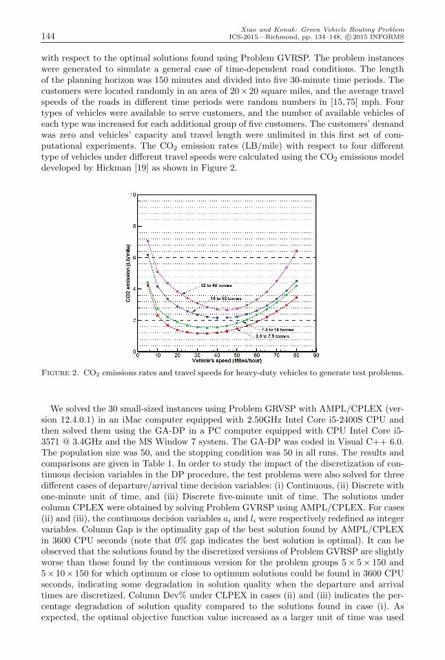
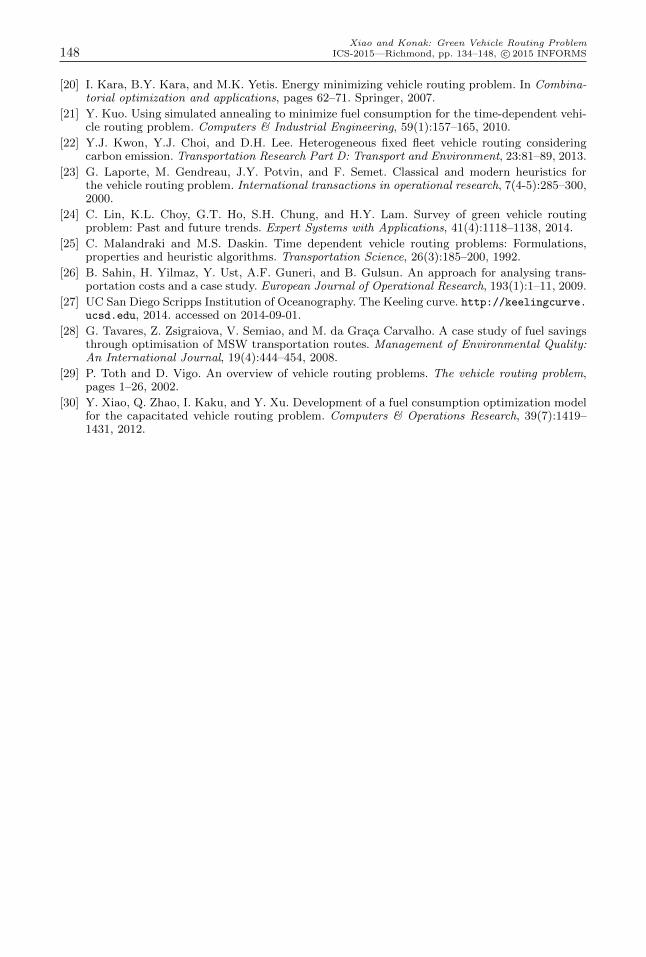
with respect to the optimal solutions found using Problem GVRSP. The problem instanceswere generated to simulate a general case of time-dependent road conditions. The lengthof the planning horizon was 150 minutes and divided into five 30-minute time periods. Thecustomers were located randomly in an area of 20× 20 square miles, and the average travelspeeds of the roads in different time periods were random numbers in [15,75] mph. Fourtypes of vehicles were available to serve customers, and the number of available vehicles ofeach type was increased for each additional group of five customers. The customers’ demandwas zero and vehicles’ capacity and travel length were unlimited in this first set of com-putational experiments. The CO2 emission rates (LB/mile) with respect to four differenttype of vehicles under different travel speeds were calculated using the CO2 emissions modeldeveloped by Hickman [19] as shown in Figure 2.
Figure 2. CO2 emissions rates and travel speeds for heavy-duty vehicles to generate test problems.
We solved the 30 small-sized instances using Problem GRVSP with AMPL/CPLEX (ver-sion 12.4.0.1) in an iMac computer equipped with 2.50GHz Intel Core i5-2400S CPU andthen solved them using the GA-DP in a PC computer equipped with CPU Intel Core i5-3571 @ 3.4GHz and the MS Window 7 system. The GA-DP was coded in Visual C++ 6.0.The population size was 50, and the stopping condition was 50 in all runs. The results andcomparisons are given in Table 1. In order to study the impact of the discretization of con-tinuous decision variables in the DP procedure, the test problems were also solved for threedifferent cases of departure/arrival time decision variables: (i) Continuous, (ii) Discrete withone-minute unit of time, and (iii) Discrete five-minute unit of time. The solutions undercolumn CPLEX were obtained by solving Problem GVRSP using AMPL/CPLEX. For cases(ii) and (iii), the continuous decision variables ai and li were respectively redefined as integervariables. Column Gap is the optimality gap of the best solution found by AMPL/CPLEXin 3600 CPU seconds (note that 0% gap indicates the best solution is optimal). It can beobserved that the solutions found by the discretized versions of Problem GVRSP are slightlyworse than those found by the continuous version for the problem groups 5× 5× 150 and5× 10× 150 for which optimum or close to optimum solutions could be found in 3600 CPUseconds, indicating some degradation in solution quality when the departure and arrivaltimes are discretized. Column Dev% under CLPEX in cases (ii) and (iii) indicates the per-centage degradation of solution quality compared to the solutions found in case (i). Asexpected, the optimal objective function value increased as a larger unit of time was used
Xiao and Konak: Green Vehicle Routing ProblemICS-2015—Richmond, pp. 134–148, c© 2015 INFORMS 145
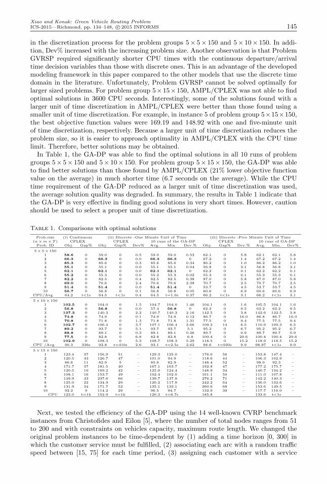
in the discretization process for the problem groups 5× 5× 150 and 5× 10× 150. In addi-tion, Dev% increased with the increasing problem size. Another observation is that ProblemGVRSP required significantly shorter CPU times with the continuous departure/arrivaltime decision variables than those with discrete ones. This is an advantage of the developedmodeling framework in this paper compared to the other models that use the discrete timedomain in the literature. Unfortunately, Problem GVRSP cannot be solved optimally forlarger sized problems. For problem group 5×15×150, AMPL/CPLEX was not able to findoptimal solutions in 3600 CPU seconds. Interestingly, some of the solutions found with alarger unit of time discretization in AMPL/CPLEX were better than those found using asmaller unit of time discretization. For example, in instance 5 of problem group 5×15×150,the best objective function values were 169.19 and 148.92 with one and five-minute unitof time discretization, respectively. Because a larger unit of time discretization reduces theproblem size, so it is easier to approach optimality in AMPL/CPLEX with the CPU timelimit. Therefore, better solutions may be obtained.
In Table 1, the GA-DP was able to find the optimal solutions in all 10 runs of problemgroups 5× 5× 150 and 5× 10× 150. For problem group 5× 15× 150, the GA-DP was ableto find better solutions than those found by AMPL/CPLEX (21% lower objective functionvalue on the average) in much shorter time (6.7 seconds on the average). While the CPUtime requirement of the GA-DP reduced as a larger unit of time discretization was used,the average solution quality was degraded. In summary, the results in Table 1 indicate thatthe GA-DP is very effective in finding good solutions in very short times. However, cautionshould be used to select a proper unit of time discretization.
Table 1. Comparisons with optimal solutions
Prob.size (i) Continuous (ii) Discrete -One Minute Unit of Time (iii) Discrete -Five Minute Unit of Time(n×m×T ) CPLEX CPLEX 10 runs of the GA-DP CPLEX 10 runs of GA-DP
Prob. ID Obj. Gap% Obj. Gap% Dev% Avg. Min. Dev.% Obj. Gap% Dev.% Avg. Min. Dev%
5× 5× 1501 58.6 0 59.0 0 0.5 59.0 59.0 0.53 62.1 0 5.8 62.1 62.1 5.82 66.3 0 66.3 0 0.0 66.3 66.3 0 67.2 0 1.4 67.2 67.2 1.43 85.3 0 85.6 0 0.3 85.6 85.6 0.34 86.2 0 1.0 86.2 86.2 1.04 55.1 0 55.1 0 0.0 55.1 55.1 0.04 56.8 0 3.1 56.8 56.8 3.15 62.1 0 62.1 0 0.0 62.1 62.1 0 62.2 0 0.1 62.2 62.2 0.16 55.2 0 55.3 0 0.0 55.3 55.3 0.02 55.3 0 0.1 55.3 55.3 0.17 82.2 0 82.5 0 0.4 82.5 82.5 0.38 87.0 0 5.8 87.0 87.0 5.88 69.0 0 70.6 0 2.4 70.6 70.6 2.38 70.7 0 2.5 70.7 70.7 2.59 51.4 0 51.4 0 0.0 51.4 51.4 0 53.7 0 4.5 53.7 53.7 4.510 56.7 0 56.8 0 0.1 56.8 56.8 0.05 60.6 0 6.9 60.6 60.6 6.9
CPU/Avg 64.2 t<1s 64.5 t<1s 0.4 64.5 t=1.0s 0.37 66.2 t<1s 3.1 66.2 t<1s 3.1
5× 10× 1501 102.5 0 104.0 0 1.5 104.7 104.0 1.46 104.1 0 1.6 105.5 104.1 1.62 56.8 0 56.8 0 0.0 57.4 56.8 0 62.2 0 9.5 62.2 62.2 9.53 137.3 0 140.3 0 2.2 140.7 140.3 2.16 142.5 0 3.8 142.6 142.5 3.84 74.8 0 74.9 0 0.1 74.9 74.9 0.12 86.7 0 16.0 86.8 86.7 16.05 70.8 0 71.8 0 1.3 71.8 71.8 1.31 77.5 0 9.4 77.5 77.5 9.46 102.7 0 106.4 0 3.7 107.1 106.4 3.66 109.3 14 6.5 110.9 109.3 6.57 89.2 0 93.7 0 5.1 93.7 93.7 5.1 95.2 0 6.7 95.2 95.2 6.78 88.8 0 89.1 0 0.3 89.1 89.1 0.26 89.7 0 0.9 89.7 89.7 0.99 77.5 0 82.8 0 6.8 82.8 82.8 6.8 100.4 0 29.6 100.4 100.4 29.610 102.9 0 108.3 0 5.3 108.7 108.3 5.29 118.5 0 15.2 118.9 118.5 15.2
CPU /Avg 90.3 336s 92.8 t=410s 2.6 93.1 t=2.5s 2.62 98.6 t=930s 9.9 98.97 t<1s 9.9
5× 15× 1501 123.4 37 156.9 51 – 129.3 125.0 – 176.0 56 – 153.8 147.4 –2 120.5 43 126.7 47 – 101.0 94.9 – 118.6 44 – 106.3 102.9 –3 86.6 11 82.9 5 – 85.6 82.9 – 148.4 52 – 98.0 92.3 –4 171.7 37 181.5 40 – 167.1 163.7 – 192.8 47 – 177.2 175.7 –5 120.5 10 169.2 42 – 125.9 124.4 – 148.9 34 – 140.7 134.2 –6 108.1 16 153.7 49 – 102.4 102.0 – 161.1 50 – 111.0 107.8 –7 149.9 43 237.6 66 – 139.7 137.9 – 276.2 71 – 142.2 140.3 –8 125.0 22 134.9 29 – 120.2 117.9 – 242.2 64 – 136.0 132.6 –9 131.9 34 171.7 52 – 135.1 133.1 – 260.6 68 – 153.6 149.5 –10 92.2 9 114.2 29 – 96.5 94.7 – 132.9 39 – 117.7 116.0 –
CPU 123.0 t=1h 152.9 t=1h 120.3 t=6.7s 185.8 133.6 t<1s
Next, we tested the efficiency of the GA-DP using the 14 well-known CVRP benchmarkinstances from Christofides and Eilon [5], where the number of total nodes ranges from 51to 200 and with constraints on vehicles capacity, maximum route length. We changed theoriginal problem instances to be time-dependent by (1) adding a time horizon [0, 300] inwhich the customer service must be fulfilled, (2) associating each arc with a random trafficspeed between [15, 75] for each time period, (3) assigning each customer with a service
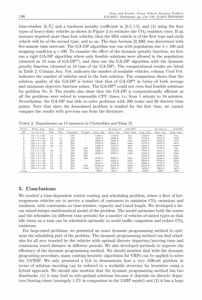
Xiao and Konak: Green Vehicle Routing Problem146 ICS-2015—Richmond, pp. 134–148, c© 2015 INFORMS
time-window [0, Ti] and a tardiness penalty coefficient in [0.5,1.5], and (4) using the fourtypes of heavy-duty vehicles as shown in Figure 2 to estimate the CO2 emission rates. If aninstance required more than four vehicles, then the fifth vehicle is of the first type and sixthvehicle will be of the second type, and so on. The time horizon [0,300] was discretized withfive-minute time intervals. The GA-DP algorithm was run with population size λ= 100 andstopping condition g= 100. To examine the effect of the dynamic penalty function, we firstran a rigid GA-DP algorithm where only feasible solutions were allowed in the population(denoted as 10 runs of GA-DP*), and then ran the GA-DP algorithm with the dynamicpenalty function (denoted as 10 runs of the GA-DP). The computational results are listedin Table 2. Column Ava. Veh. indicates the number of available vehicles, column Used Veh.indicates the number of vehicles used in the best solution. The comparison shows that thesolution quality of the GA-DP is better that that of GA-DP* in terms of both averageand minimum objective function values. The GA-DP* could not even find feasible solutionsfor problem No. 9. The results also show that the GA-DP is computationally efficient asall the problems were solved in reasonable CPU times, i.e, from 1 minute to 18 minutes.Nevertheless, the GA-DP was able to solve problems with 200 nodes and 60 discrete timepoints. Note that since the formulated problem is studied for the first time, we cannotcompare the results with previous one from the literature.
Table 2. Experiments on 14 instances in Christofides and Eilon [5]
Prob. Prob. size Ava. Used 10 runs of GA-DP* 10 runs of GA-DP
ID n×m×T Veh. Veh. Capacity Length Avg. obj. Min. obj. Avg. time Avg. obj. Min. obj. Avg. time
1 50× 5× 60 7 7 160 – 1187.1 1148.9 31s 1189.5 1099.1 51s2 75× 5× 60 13 11 140 – 1824.7 1696.9 70s 1728.0 1615.6 159s3 100× 5× 60 12 10 200 – 2038.0 1925.9 182s 2108.7 1953.8 177s4 150× 5× 60 16 14 200 – 2724.2 2601.2 444s 2772.2 2555.0 567s5 199× 5× 60 20 18 200 – 3429.5 3353.0 452s 3444.1 3115.0 1055s6 50× 5× 60 7 6 160 200 1296.7 1245.6 54s 1251.7 1178.5 44s7 75× 5× 60 13 11 140 160 1888.3 1750.0 109s 1705.0 1631.4 160s8 100× 5× 60 11 9 200 230 2088.0 1965.5 149s 1939.0 1814.0 199s9 150× 5× 60 15 13 200 200 – – – 2794.2 2536.8 545s10 199× 5× 60 21 18 200 200 3178.4 3099.5 554s 3210.3 3028.7 628s11 120× 5× 60 11 9 200 – 3905.1 3594.6 279s 3943.8 3700.2 325s12 100× 5× 60 12 10 200 – 2034.0 1795.6 153s 2088.5 1773.8 134s13 120× 5× 60 12 10 200 720 10304.2 4007.5 250s 6019.9 3879.4 313s14 100× 5× 60 22 10 200 1040 2047.8 1861.4 227s 1958.0 1800.8 347s
Avg 2919 2311 227 2582 2263 336
5. Conclusions
We studied a time-dependent vehicle routing and scheduling problem, where a fleet of het-erogeneous vehicles are to service a number of customers to minimize CO2 emissions andtardiness, with constraints on time-window, capacity and travel length. We developed a lin-ear mixed-integer mathematical model of the problem. The model optimizes both the routesand the schedules (in different time periods) for a number of vehicles of mixed types so thatidle times on a tour can be scheduled optimally to avoid traffic congestion and reduce CO2
emissions.For large-sized problems, we presented an exact dynamic programming method to opti-
mize the scheduling part of the problem. The dynamic programming method can find sched-ules for all arcs traveled by the vehicles with optimal discrete departure/arriving time andcontinuous travel distance in different periods. We also developed methods to improve theefficiency of the dynamic programming method. We should mention that with the dynamicprograming procedure, many existing heuristic algorithms for VRPs can be applied to solvethe GVRSP. We only presented a GA to demonstrate how a very difficult problem interms of solution encoding can be reduced to a workable structure for heuristics using ahybrid approach. We should also mention that the dynamic programming method has twodrawbacks: (1) it may lead to sub-optimal solutions because it depends on discrete depar-ture/leaving times (averagely 1.5% in comparison to the LMIP model) and (2) it has a large
Xiao and Konak: Green Vehicle Routing ProblemICS-2015—Richmond, pp. 134–148, c© 2015 INFORMS 147
memory requirement. However, these drawbacks will be insignificant for real-life applica-tions. We developed a genetic algorithm with dynamic programming to solve the GVRSPwith near-optimal solutions.
Acknowledgement
This work is partly supported by the National Natural Science Foundation of China underGrants No. 71271009.
References[1] The International Energy Agency. CO2 emissions from fuel combustion—highlights
(2012 edition). https://www.iea.org/co2highlights/co2highlights.pdf, 2012. accessed on2014-02-06.
[2] M. Barth and K. Boriboonsomsin. Real-world carbon dioxide impacts of traffic congestion.Transportation Research Record: Journal of the Transportation Research Board, 2058(1):163–171, 2008.
[3] T. Bektas and G. Laporte. The pollution-routing problem. Transportation Research Part B:Methodological, 45(8):1232–1250, 2011.
[4] H.K. Chen, C.F Hsueh, and M.S. Chang. The real-time time-dependent vehicle routing prob-lem. Transportation Research Part E: Logistics and Transportation Review, 42(5):383–408,2006.
[5] N. Christofides and S. Eilon. An algorithm for the vehicle-dispatching problem. OperationalResearch Quarterly, pages 309–318, 1969.
[6] G.B. Dantzig and J.H. Ramser. The truck dispatching problem. Management science, 6(1):80–91, 1959.
[7] N. Dellaert and J. Jeunet. Solving large unconstrained multilevel lot-sizing problems usinga hybrid genetic algorithm. International Journal of Production Research, 38(5):1083–1099,2000.
[8] E. Demir, T. Bektas, and G. Laporte. An adaptive large neighborhood search heuristic for thepollution-routing problem. European Journal of Operational Research, 223(2):346–359, 2012.
[9] E. Demir, T. Bektas, and G. Laporte. The bi-objective pollution-routing problem. EuropeanJournal of Operational Research, 232(3):464–478, 2014.
[10] E. Demir, Tolga Bektas, and G. Laporte. A review of recent research on green road freighttransportation. European Journal of Operational Research, 237(3):775–793, 2014.
[11] B. Eksioglu, A.V.Vural, and A. Reisman. The vehicle routing problem: A taxonomic review.Computers & Industrial Engineering, 57(4):1472–1483, 2009.
[12] S. Erdogan and E. Miller-Hooks. A green vehicle routing problem. Transportation ResearchPart E: Logistics and Transportation Review, 48(1):100–114, 2012.
[13] E. Ericsson, H. Larsson, and K. Brundell-Freij. Optimizing route choice for lowest fuelconsumption–potential effects of a new driver support tool. Transportation Research Part C:Emerging Technologies, 14(6):369–383, 2006.
[14] M. Figliozzi. Vehicle routing problem for emissions minimization. Transportation ResearchRecord: Journal of the Transportation Research Board, 2197(1):1–7, 2010.
[15] A. Franceschetti, D. Honhon, T. Van Woensel, T. Bektas, and G. Laporte. The time-dependentpollution-routing problem. Transportation Research Part B: Methodological, 56:265–293, 2013.
[16] D.R. Gaur, A. Mudgal, and R.R. Singh. Routing vehicles to minimize fuel consumption. Oper-ations Research Letters, 41(6):576–580, 2013.
[17] D.E. Goldberg and R. Lingle. Alleles, loci, and the traveling salesman problem. In Proceedingsof the International Conference on Genetic Algorithms and Their Applications, pages 154–159.Lawrence Erlbaum, Hillsdale, NJ, 1985.
[18] B.L. Golden, S. Raghavan, and E.A. Wasil. The Vehicle Routing Problem: Latest Advances andNew Challenges: latest advances and new challenges, Operations Research/Computer ScienceInterfaces Series, Volume 43. Springer, 2008.
[19] J. Hickman, D. Hassel, R. Joumard, Z. Samaras, and S. Sorenson. Methodology for calculatingtransport emissions and energy consumption. Transport Research Laboratory, Project ReportSE/491/9 1999.
Xiao and Konak: Green Vehicle Routing Problem148 ICS-2015—Richmond, pp. 134–148, c© 2015 INFORMS
[20] I. Kara, B.Y. Kara, and M.K. Yetis. Energy minimizing vehicle routing problem. In Combina-torial optimization and applications, pages 62–71. Springer, 2007.
[21] Y. Kuo. Using simulated annealing to minimize fuel consumption for the time-dependent vehi-cle routing problem. Computers & Industrial Engineering, 59(1):157–165, 2010.
[22] Y.J. Kwon, Y.J. Choi, and D.H. Lee. Heterogeneous fixed fleet vehicle routing consideringcarbon emission. Transportation Research Part D: Transport and Environment, 23:81–89, 2013.
[23] G. Laporte, M. Gendreau, J.Y. Potvin, and F. Semet. Classical and modern heuristics forthe vehicle routing problem. International transactions in operational research, 7(4-5):285–300,2000.
[24] C. Lin, K.L. Choy, G.T. Ho, S.H. Chung, and H.Y. Lam. Survey of green vehicle routingproblem: Past and future trends. Expert Systems with Applications, 41(4):1118–1138, 2014.
[25] C. Malandraki and M.S. Daskin. Time dependent vehicle routing problems: Formulations,properties and heuristic algorithms. Transportation Science, 26(3):185–200, 1992.
[26] B. Sahin, H. Yilmaz, Y. Ust, A.F. Guneri, and B. Gulsun. An approach for analysing trans-portation costs and a case study. European Journal of Operational Research, 193(1):1–11, 2009.
[27] UC San Diego Scripps Institution of Oceanography. The Keeling curve. http://keelingcurve.ucsd.edu, 2014. accessed on 2014-09-01.
[28] G. Tavares, Z. Zsigraiova, V. Semiao, and M. da Graca Carvalho. A case study of fuel savingsthrough optimisation of MSW transportation routes. Management of Environmental Quality:An International Journal, 19(4):444–454, 2008.
[29] P. Toth and D. Vigo. An overview of vehicle routing problems. The vehicle routing problem,pages 1–26, 2002.
[30] Y. Xiao, Q. Zhao, I. Kaku, and Y. Xu. Development of a fuel consumption optimization modelfor the capacitated vehicle routing problem. Computers & Operations Research, 39(7):1419–1431, 2012.