Green Technology Adoption: An Empirical Study of the

Southern California Garment Cleaning Industry ∗

Bryan Bollinger, Stanford University

September 6, 2010

JOB MARKET PAPER

Abstract

New technologies are crucial in dealing with the problem of air and water pollution, which

is an increasingly important issue with serious health and environmental consequences. Adop-

tion of environmentally friendly technologies can be slow if the new technologies are not supe-

rior in terms of the firms’ private incentives, if firms have long equipment replacement cycles,

or if firms do not have sufficient information to evaluate whether or not a switch to a green

technology is in their private interests. To evaluate these potential explanations and the policies

designed to address them, this paper uses importance sampling to estimate a dynamic durable

good replacement model for garment cleaning firms in southern California. The standard dry

cleaning technology uses perchloroethylene (perc), a toxic air and ground contaminant, and

the alternative technologies have seen only limited adoption to date. The model controls for

and exploits changing legislation to estimate the effect of fees and incentives on green equip-

ment purchases, as well as the effect of product demonstrations. The estimated model is used

to compare the predicted adoption and entry/exit decisions by firms under different regula-

tory regimes. While the model is tailored to the garment cleaning industry, it can be adapted

to other applications involving the diffusion of socially better technologies.

∗I would like to thank Harikesh Nair, Sridhar Narayanan, and Peter Reiss for their helpful comments. I would like

to especially thank Wesley Hartmann for his invaluable support and guidance throughout. All remaining mistakes are

my own.

1 Introduction

The adoption of new, cleaner technologies is essential in reducing pollution. Even if the technolo-

gies have already been developed, the empirical technology diffusion literature has demonstrated

that the diffusion of new technologies can be slow (Bass 1969, Mahajan, Muller & Bass 1990, Han-

nan & McDowell 1984, Mulligan 2003, Baker 2001, Engers, Hartmann & Stern 2009). There are a

variety of potential explanations for slow adoption: i) firms do not realize the full societal bene-

fits of using the green technology and the green technology is not superior in terms of the firms’

private incentives; ii) firms may have long equipment replacement cycles which have slowed the

migration to a socially and privately better technology; or iii) firms may not have sufficient in-

formation to evaluate whether or not a switch to a green technology is in their private interests.1

Government intervention is often used to expedite the adoption of the cleaner technologies, in

order to reduce the difference in the private and social values of adoption. Firm decisions are

therefore affected by a mix of firm variables including product quality, pricing and advertising in

concert with government pricing, advertising, and possibly regulation.

When there are important dynamics to consider, as in the case of durable goods, it is becom-

ing more common in the marketing and economics literature to structurally model an agent’s

decision to adopt a new technology (Gowrisankaran & Stavins 2004, Tucker 2008, Gordon 2009).

A structural analysis of firms’ adoption decisions allows for the estimation of policy-invariant

profit function parameters which can be used to assess the different tools used by policymakers,

or firms, to expedite the adoption of the different technologies. The application studied here is

garment cleaning, which i) involves the purchase of durable goods and faces just such a mix of

policies to drive adoption; ii) has readily available public data; and iii) has experienced variation

in policies over time that have altered both current variables and the expectations of the future,

which drive the identification of dynamic models.

I construct and estimate a single agent, dynamic durable good adoption model adapted from

Rust (1987) that explicitly solves for firms’ solutions to their dynamic optimization problems, as is

1The theory literature on technology adoption has demonstrated that uncertainty in new technologies may createbarriers to adoption, which are even larger in the case of durable goods (Jensen 1982, Farzin, Huisman & Kort 1998,Doraszelski 2001).

1

common in the literature (Nair 2007, Hartmann & Nair 2009, Smith 2010).2 I estimate the structural

primitives of the model using importance sampling (Ackerberg 2009) as done in Hartmann (2006),

Bajari, Hong & Ryan (2009), and Goettler & Clay (2010) in order to include rich heterogeneity

which I would expect due to the environmental nature of the application. Potential reasons for

heterogeneity in profits when using different types of equipment include differences in marginal

costs or in the prices firms are able to charge consumers for cleaning since the demand for cleaning

equipment reflects the demand for garment cleaning. This is the only application of importance

sampling of which I am aware that includes entry and exit in a dynamic setting with heterogeneity

and controls for the endogeneity of the initial market conditions regarding which agents are in the

market at the start of the panel.

In this paper, I use the exogenously changing environmental policies in southern California

to help identify the distribution of heterogeneity in firms’ profit parameters, which I then use to

evaluate the California policies with several alternatives. Although I use California data, I am able

to assess how outcomes would have changed if other policies, such as those in a neighboring state,

Oregon, were used instead. The dynamic, structural model allows firms and/or governments

to predict green technology adoption under varying combinations of pricing for equipment and

inputs, product demonstrations, and potentially, outright bans. The two examples, California and

Oregon, allow me to compare one set of policies that uses a mixture of policy tools including a ban

on the polluting technologies with another that only uses a market-based incentive (a tax on the

polluting solvent). To preview my results, both sets of policies lead to increased adoption of the

green technologies, and while there is a large effect of demonstration sites on the adoption of the

demonstrated technology, most of this extra adoption is by firms who would have adopted one of

the other green technologies. There is less exit under California’s policies which is mostly offset

by reduced entry.

The rest of the paper is organized as follows: In the next section, I provide background regard-

ing the garment cleaning industry and the policies designed to phase out perc, and in section 3 I

describe the data. My model and estimation strategy are outlined in section 4 and the results are

2Two-stage methods such as Hotz & Miller (1993) and Bajari, Benkard & Levin (2007) are unsuited to this applicationsince there are a limited number of adoptions of the green technologies, significant heterogeneity, and lots of variationin the policies.

2

presented in section 5. Section 6 provides a discussion of the results and I use the structural pa-

rameter estimates to perform counterfactual market simulations which are presented in 7. Section

8 concludes.

2 Background

2.1 Industry Background

Laundry services and garment cleaning is a $22.6 billion dollar per year industry, according to

the 2007 U.S. Census Bureau’s Annual Services Survey (Hambric 2008). The standard technology

used in garment cleaning requires the use of perchloroethylene (perc), a toxic, cancer-causing air

and ground contaminant used by approximately 28,000 U.S. dry cleaners nationwide according

to the Environmental Protection Agency (EPA). The issue is of such importance that the State

Coalition for Remediation of Drycleaners was established in 1998, with support from the EPA, in

order to aid in the development of remediation programs to clean up contamination caused by the

use of perc.3 A document was released by the EPA in 1992 summarizing the hazards associated

with exposure to perc, and since then the use of the chemical has come under more and more

scrutiny. Currently, the EPA is considering whether to compel dry cleaners to phase out perc

nationwide, according to a recent article in the Washington Post.4 The California Dry Cleaning

Industry Technical Assessment Report was published in 2006 as part of the 1993 Airborne Toxic

Control Measure for Emissions of Perchloroethylene from Dry Cleaning Operations and provides

a detailed description of the California garment cleaning industry(Fong, Chowdhury, Houghton,

Komlenic & Villalobos 2006). The California Air Resources Board (CAARB) 2003 facility surveys

estimated that there were around 5040 cleaners, 4670 of which used perc.

Most types of equipment that use perc (and most of the alternative solvents) are closed-loop

machines meaning that the washing, extraction and drying of the garments all occur within the

3Thirteen states are members of the coalition.4Washington Post, Wednesday, April 8, 2009, page A03. http://www.washingtonpost.com/wp-

dyn/content/article/2009/04/07/AR2009040703748.html

3

same machine. To dry the clothes, air is pulled in from outside and then released. Different con-

trol methods have been developed to reduce the emission of perc into the air during the drying

process, primarily refrigerated condensers which cool the air before emitting it back into the at-

mosphere. Perc emissions also occur at the end of the cleaning cycle when the drum is opened to

remove the clothes. Secondary control methods help to trap perc before the clothes are removed.

However, despite the control technologies, a significant amount of perc still escapes during the

cleaning process.

Although the majority of cleaners use perc equipment, alternative cleaning technologies are

available. Some equipment use hydrocarbon or fluorocarbon solvents (also known as mineral spir-

its) instead of perc. The process is quite similar to perc cleaning. There are a few other solvents

used as perc replacements but most of them also have health or environmental risks associated

with them. Decamethylcyclopentasiloxane, the chemical found in the silicon-based GreenEarth

solvent has been found to have similar efficacy to perc and has low solubility in water, thus reduc-

ing water pollution.5

Carbon dioxide (CO2) and wet cleaning are considered to be the cleanest perc alternatives.

CO2 cleaning is a closed-loop process that uses pressurized carbon dioxide, a non-toxic, naturally-

occurring gas. The liquid CO2 and detergent are circulated through the clothes with the use of jets

inside the cleaning equipment. The dirt is removed with the CO2 during the drying process. It

is a gentle cleaning process with a longer drying cycle than perc cleaning. There are three U.S.

manufacturers of CO2 equipment.

Wet cleaning was developed in 1991 and requires special equipment and a higher level of

control throughout the cleaning process that the other types of cleaning. The washer and dryer

are separate pieces of equipment, and like CO2 cleaning, the drying process is longer than for

perc cleaning. Unlike when using the previously discussed technologies, tensioning equipment is

needed to restore the clothes after wet cleaning to their original shape. More training is required

for employees when using wet cleaning equipment in order to understand the process and ensure

efficacy.

5Research is ongoing as to whether it is a carcinogen.

4

The road to perc regulation began in 1991 when the CAARB determined that perc is a toxic

air contaminant which falls under California’s Toxic Air Contaminant Identification and Control

Program. In 1993, the CAARB adopted the Airborne Toxic Control Measure for Emissions of Perc

from Dry Cleaning Operations (Dry Cleaning ATCM) and the Environmental Training Program

for perc dry cleaning operations. These measures set new requirements for cleaners in an effort to

reduce air contamination.

The South Coast Air Quality Management District (SCAQMD) is the air pollution control

agency for all of Orange County and the urban portions of Los Angeles, Riverside and San Bernardino

counties. It has the largest number of cleaners in the state and has been very aggressive in its plan

to phase out perc, even more so than the CAARB. The SCAQMD is looking to eliminate the use of

perc machines by the end of 2020, recognizing the durable nature of the equipment in its phase-

out plan. SCAQMD Rule 1421 was first passed on December 9, 1994, but the final version was

updated December 6, 2002. It states that ”On or after January 1, 2003, an owner or operator of a

new facility may not operate a perchloroethylene dry cleaning system. On or after December 6,

2002, an owner or operator of an existing facility shall be allowed to operate its perchloroethylene

dry cleaning system(s) until the end of its useful life6 and, upon replacement, shall be allowed to

operate no more than one perchloroethylene dry cleaning system per facility until December 31,

2020.”

In December 2002, the SCAQMD also instituted a grant program for dry cleaners willing to

upgrade to cleaner technologies, including carbon dioxide, wet cleaning, hydrocarbon and Gree-

nEarth. There is no consensus as to which technologies should be labeled as green. In this paper, I

refer to all non-perc cleaning technologies as green technologies although carbon dioxide and wet

cleaning are the most environmentally-friendly. The SCAQMD grants give $10,000 to dry clean-

ers willing to switch to carbon dioxide cleaning,7 $10,000 to switch to wet cleaning, and $5,000 to

switch to hydrocarbon or GreenEarth.8

6The “useful life” of the equipment is something that came under rigorous debate between the SCAQMD and theCalifornia Cleaners Association(CCA), the SCAQMD wishing to set the useful life at ten years, the CCA at 20. A 15year useful life was the compromise.

7The CO2 incentive was recently changed to $20,000.8The grants for GreenEarth were soon discontinued, in 2003, and hydrocarbon grants were discontinued in 2007.

5

In addition, the state of California passed Assembly Bill 998 (AB 998) in August 2004 which

established the CAARB’s own non-toxic dry cleaning incentive program. The CAARB incentive

program gives $10,000 grants to dry cleaners using perc if they are willing to switch to either

carbon-dioxide or wet cleaning technologies. The Air Resources Board plans to completely phase

out perc dry cleaning machines state-wide by the year 2023. The CAARB grants were not available

for the purchase of hydrocarbon or GreenEarth equipment. The majority of the funding for the

CAARB dry cleaning program comes from fees imposed on the purchase of perc solvent (under

AB 998). The fees began in 2004 at three dollars per gallon of solvent and increase by one dollar

annually until 2013, when they are $12 per gallon.

AB 998 also requires the CAARB to use its funds to support a demonstration program which

provides dry cleaners with the opportunity to learn about green cleaning technology, primarily

wet cleaning, at various locations across California. Technical assistance and training are pro-

vided through the program in an attempt to reduce the costs and supply information regarding

the benefits and overall effectiveness of carbon dioxide and wet cleaning technologies, although

I only observe wet cleaning demonstration sites in southern California. The sites are usually gar-

ment cleaning firms who receive a subsidy to become a demonstration site. On one day, other

cleaners are invited to come walk through the wet cleaning process to see for themselves how to

use the new cleaning method and how effective the cleaning is. These sites have the ability to re-

duce uncertainty in the new technologies or may lead firms to update their prior beliefs regarding

the effectiveness of the new technology. The time-dependent geographic proximity of demonstra-

tion sites (as they are established) to potential adopters can be used to estimate the barriers to

adoption which are eliminated by the provision of this information and training. According to the

CAARB website, ”Demonstration sites ultimately will, in time, create the regional and statewide

infrastructure necessary for the long-term diffusion of these technologies.” Lastly, on January 25,

2007, California legislators amended the Dry Cleaning ATCM. The amended ATCM prohibits the

sale or lease of new perc dry cleaning machines beginning on January 1, 2008.9 This was a drastic

policy shift away from the gradual phase-out plan and is reflected in the data.

9In addition, it forbids the use of existing perc machines at co-residential facilities and requires the removal of percmachines that are 15 years or older by July 1, 2010. All other perc machines must be removed from service once theybecome 15 years old or by January 1, 2023, whichever is sooner. The law also requires expanded record keeping by percfacilities and manufacturers.

6

According to the president of the California Cleaners Association (CCA), the cleaners have

been working with the California Air Quality Management Districts across the state to try to limit

the financial costs of the phase-out. However, the many changes in the regulations were unan-

ticipated by the cleaners who had limited ability to alter the legislation. Even the compromise

of 15 years as the regulated useful life of perc cleaning equipment is now potentially going to be

altered by the San Francisco Bay Area AQMD which is considering legislation to change the legal

useful life of perc equipment to 10 years. The cleaners are being forced into the transition away

from perc, and the CCA is now concerned that new legislation might force cleaners away from the

use of hydrocarbon cleaning as well, which is considered by many cleaners to be the most cost-

effective technology after perc, according to anecdotal evidence. According to the CCA, cleaners

are already being forced out of business by the new regulations and more restrictions will make

the problem considerably worse.

3 Data

3.1 Data Sources

Permits This paper uses permiting data available through the SCAQMD. I have the dates at

which all permits were granted to perc and hydrocarbon dry cleaners in the SCAQMD which

encompasses most of southern California. These permit data also track changes of firm ownership

since new owners need to re-permit their equipment. A total of 14,877 permit applications by

4,270 cleaners were filed with the SCAQMD between 1956 and 2008, resulting in 13,172 permits.

In this analysis I treat cleaners after an ownership change as the same firm. Most of the cleaners

that appear in the SCAQMD data have perc equipment but some fraction of the cleaners have

equipment that uses hydrocarbon or other petroleum solvent.

The data include each facility’s name, address and phone number, as well as the type of equip-

ment, whether a permit was issued (usually the case) and the date the permit was issued. Since

1996, the SCAQMD has also kept track of whether facilities have gone out of business or become

7

inactive for some other reason. I also have access to permit diary files which track firm actions in

1982 and later. I can use these data to determine whether firms exited the market prior to 1996,

assuming that firms that inactivated a permit with no new permit left the market. Unfortunately,

these diary files are not complete. If a firm is included in the data and has not purchased equip-

ment since before 1983, I assume it is inactive and use the last SCAQMD inspection date as the

exit date. It is important to include the firms that exited to make sure I do not underestimate the

probability of exit under the new policies.10

Green Cleaners The data on cleaners using wet, carbon dioxide or GreenEarth cleaning come

from a variety of sources. The first source is the list of SCAQMD grant recipients. The grants

began in 2003 and included incentives for adopting hydrocarbon, wet cleaning, carbon dioxide,

and GreenEarth cleaning technologies. The GreenEarth grants were discontinued after one year

and the hydrocarbon grants were eliminated after 2007. Only the incentives for wet cleaning

and carbon dioxide are still in place, and in 2007, the carbon dioxide grants were retroactively

increased to $20,000. There were 596 SCAQMD grant recipients by the end of 2008.

The second data source is the list of CAARB grant recipients. In 2005, the CAARB began their

garment cleaning grant program, but only for cleaners switching to wet cleaning and carbon diox-

ide. In addition, cleaners taking the CAARB grants are required to remove their perc equipment

from the facility and commit to not purchasing perc equipment in the future. There have been 85

recipients between 2005 and 2008 from all of California.

In addition, a list of green cleaners was acquired from the Urban & Environmental Policy

Institute (UEPI), a community oriented research and advocacy organization based at Occidental

College in Los Angeles, CA. The UEPI website allows consumers to search for green cleaners

(which they define to be wet or carbon dioxide cleaners) that are within a given radius of a user-

provided address. Their database includes 166 wet and carbon dioxide cleaners in California. The

ability for consumers to search for cleaners using the cleaner technologies is one potential benefit

10I first remove superfluous actions when a firm inactivates and actives a piece of equipment in the same or adjacentyears, presuming it is the same piece of equipment. I also remove firms which I assume are inactive but cannot establishan exit date, which is the case for 23 firms. I also remove a few firms which do not do anything for a span of at leastthirty years, and I therefore assume I have missing exit actions. There are 6 of these firms.

8

to adoption.

Finally, I use the SCAQMD permit diary files to identify if a permit was inactivated in order

to switch to a different technology. This identification of green cleaners depends on the diary de-

scription variable and provides me with information for cleaners who purchased green equipment

before the incentives were available.

Demonstration Sites Under the CAARB demonstration program, there were 26 demonstrations

of either wet cleaning or carbon dioxide cleaning before 2009 at 18 different sites in California.

Of these demonstration sites, 17 of them were cleaners who chose to become demonstration sites

and received a CAARB incentive to purchase wet or carbon dioxide cleaning equipment and an

additional incentive to become a demonstration site. The UEPI also sponsors a green cleaning

demonstration program, in cooperation with the CAARB. There have been 30 total demonstra-

tion sites in California, thirteen of which are located in the SCAQMD region and which occurred

during my period of study (1999-2008). These thirteen demonstration sites were all wet cleaning

locations.

Other Data I include firm data from Reference USA to explain some of the heterogeneity in

profit parameters across firms. These data include variables from 2008 including sales, number of

employees, credit rating, and square footage of the facility. Except for credit rating, the variables

are in bins of discrete size with only a few realized values for each variable, which limits their

value. I also only have data for currently active firms. I merged the cleaners from the above data

with the Reference USA data, which include garment cleaning drop-off locations in addition to

cleaners who do their own cleaning. There were 2,225 matches; the Reference USA data only

include information for cleaners which are currently active. There are 2,701 cleaners who do not

appear in the permitting data; most likely, they are cleaners who outsource their cleaning.

In addition to the firm-specific variables available through Reference USA, I include zip-code

level variables which may explain heterogeneity in demand for garment cleaning or green clean-

ing specifically. These variables include income, family size, ethnicity and age, as well as variables

9

that may indicate a preference for green alternatives, such as the fraction of commuters who car-

pool, walk or use public transportation and the relative number of hybrid vehicle purchases. These

data were assembled from American Factfinder, Sourcebook America and a proprietary dataset on

vehicle registrations from R.L. Polk and Company.

3.2 Data Summary

I combine the different data files by doing an address match between firms in the SCAQMD data

and in the other data sets. Of the different technologies, my data include cleaners which have

adopted hydrocarbon, wet, carbon dioxide, and GreenEarth cleaning equipment. The estimated

costs for these different types of equipment can be found in Table 1, along with average annual

operating costs exclusive of labor.11

I geocode the firm and demonstration site locations to calculate the distances between the firms

and all of the demonstration sites in every given year. I limit the analysis to the years 1999-2008

for a variety of reasons. First, I do not have complete facility action data before 1996. Second,

this is after firms are aware of the issues surrounding perc cleaning since the period follows the

CAARB’s formal classification of perc as a toxic air contaminant in 1991, the 1993 passing of the

CAARB ATCM, and the SCAQMD’s passing of the original version of Rule 1421 in 1994. Finally,

it is desirable because CAARB Rule 1421 forbids the use of transfer or vented perc machines after

1998, and as a result, I see a relatively large number of firms (388) exit the market in that year. Since

I cannot identify which perc machines are of these types, I cannot control for this strict command-

and-control regulation since there is no way to determine if firms that bought new equipment or

exited the market did so because of the mandate. In the analysis, I do still assume a stationary

equilibrium in 1999, which is reasonable considering that firms can convert their vented machines

to closed loop machines.

11More detail can be found in the CAARB California Dry Cleaning Industry Technical Assessment Report. Opera-tional costs follow the same trends as the machinery costs: Carbon dioxide cleaning has high capital and operationalcosts but wet cleaning actually has lower costs than traditional perc cleaning. However, this does not account for the ex-tra training required to use the greener technologies or the fact that wet cleaning is more labor intensive than traditionaldry cleaning.

10

I use the permit data to compute the age of each cleaner’s equipment over time. I keep track

of the age of their most current equipment only. There are 3,534 cleaners in the combined data

set, but not all of these cleaners are active at the same time. In any year, there are just over 3,000

active cleaners. To get a sense of the current industry size and level of green technology adoption,

Table 2 breaks down the technology used by those cleaners which were active at the end of 2008.

In addition, it includes the average distance to the nearest demonstration site.12 While there has

been considerable adoption of hydrocarbon cleaning, and some adoption of wet cleaning, there

has been little adoption of GreenEarth and only four firms have adopted carbon dioxide. Not

surprisingly, the average distance to the nearest demonstration site is smaller for cleaners who are

now using wet (or carbon dioxide) cleaning.

Due to the limited number of observations for cleaners choosing the cleaner technologies, it

is useful to tabulate the cleaners’ actions by current equipment type and age, as well as by year.

Table 3 shows how the actions of cleaners depend on the current type of equipment owned. This

table will determine what I can actually identify in estimation. Since I do not observe cleaners

who have purchased wet, carbon dioxide or GreenEarth equipment exit the market or purchase

other equipment in subsequent years, I will be restricted in my ability to separately identify the

utility of purchasing equipment from the utility of utilizing the equipment.

Table 4 separates the actions by the age of the previous equipment. There are more purchase

actions than I would expect when the age of the existing equipment is low. Some of this is likely a

result of assuming new permits are for new equipment, when in fact the permitted equipment may

be used. I try to limit these errors by ignoring new permits if I observe the previous equipment

being deactivated in the permit diary files. Also, according to garment cleaning facility survey

results in the 2006 CAARB technical assessment report, 89% of machines are bought new and 96%

of owners said they would buy a new machine in the future, these errors should be kept to a

minimum and not have a discernable impact on the results.

Another explanation for the large number of new equipment purchases when the previous

equipment is only a few years old is the changing regulations. In particular, the CAARB restriction

12Other than themselves if they became a demonstration site.

11

against perc purchases after 2007 likely led cleaners to purchase new equipment when they may

have otherwise waited. Many of the perc equipment purchases when the previous equipment was

relatively new took place in 2007. A final explanation could be that age simply does not matter

much, either because there is limited machine depreciation or because there is relatively efficient

secondary market for used equipment, in which case depreciation would be reflected in the scrap

value upon exiting as well as when cleaners use their old equipment.

Table 5 shows which actions occurred in which years. There are a few features of the data that

are notable. One is that in 2003, the year in which both the 2004 Assembly Bill was announced

and the SCAQMD incentives began, I observe many more green equipment purchases. There

appears to be a large effect of the SCAQMD and CAARB incentives in the years they are offered; in

particular, most GreenEarth purchases occur in 2003, the only year the incentives were available;

there is also a drop in the average age of firms who buy wet cleaning equipment and exit the

market in this year, and the age for firms who buy GreenEarth equipment is also at its lowest

point.

One of the most striking observations in the data is what occurred in 2007 when it was an-

nounced that cleaners would not be able to purchase perc equipment in later years. There is a

large spike in perc purchases in 2007. One would expect some increase since it was announced at

the beginning of the year that it is the last year to purchase perc equipment, but the magnitude

of the increases seem to indicate that there are some firms who are very reluctant to switch tech-

nologies. The average age of firms buying perc equipment drops by two years, which provides

evidence that firms are purchasing perc before they would have done so due to this new regula-

tion forbidding perc purchases after that year. Hydrocarbon purchases also experience a modest

spike in this year, possibly since this was the last year the hydrocarbon grants were available.

12

4 Model and Estimation

4.1 Firm Profits

I expect firm profits to depend on the type of technology used. Differences in profits across the

technology types could be from a variety of sources including equipment purchase costs, fixed

costs, operating costs such as solvent and electricity use, and markup which will depend on con-

sumers’ willingness to pay for cleaning performed by that type of equipment. A firm’s ability

to charge a different markup depending on the type of technology would imply quality or per-

ceived quality differences between the technologies. The firms which have adopted carbon diox-

ide cleaning are all located in affluent areas where consumers may be willing to pay a premium

for environmentally friendly cleaning. On the other hand, wet cleaning, although environmen-

tally friendly, may have negative connotations if consumers are concerned about the efficacy of

the cleaning or potential damage to the clothes by this more radical technology.

Because of the large capital costs and the durable nature of cleaning equipment, as well as the

changing regulatory environment, cleaners are modeled as forward-looking profit maximizers.

The model developed in this paper is a single-agent, regenerative optimal stopping model adapted

from Rust (1987), allowing for entry and exit. In each period, a dry cleaner faces the decision

whether or not to remain in the market, whether to invest in new machinery, and if so, what type

to invest in. Let the choice-specific profit function for cleaner i be given as:

π(xiτ , jiτ , ψt, sit|βi) + εijτ , (1)

where jiτ is the choice at time τ . The choice set Ct(τ) includes the following choices: j = 0 (exit), 1

(no investment), 2 (purchase perc equipment), 3 (purchase hydrocarbon equipment), 4 (purchase

wet cleaning equipment), 5 (purchase carbon dioxide equipment), 6 (purchase GreenEarth equip-

ment). After 2007, the choice to purchase perc equipment is removed from the choice set. I assume

that the unobserved profit shock, εijτ , enters the profit function linearly and follows an iid type 1

extreme value distribution.13

13Since I impose the condition of conditional independence of the unobservable state variable I assume that all de-

13

I define x = {e, w, t} as the vector of observable state variables including e, the current technol-

ogy used by the firm (or if the firm is a potential entrant), equipment age w which I define as the

number of years since purchase within which the equipment is operating (w = 1 if the equipment

is new), and the year t. A firm’s technology and the age of its equipment evolve according to the

following laws of motion, where Pt is a dummy variable indicating an equipment purchase:

wt = wt−1 + 1 if Pt = 0 (2)

et = et−1 if Pt = 0

wt = 1 if Pt = 1.

et = jt if Pt = 1.

This simply says that the equipment age increases by one and the type of equipment stays the same

if no new equipment is purchased, and the age is immediately reset to one and the equipment type

changes to the purchased equipment if new equipment is purchased. This assumes that cleaners

can use newly purchased equipment immediately. The age variable is set to one for potential

entrants, and in each period I assume there is a new set of potential entrants.

Time enters the firms’ value functions due to the changing environmental legislation, ψt(e, τ) =

{ft(e, τ), gt(e, τ), Ct(τ)}, which includes the equipment-specific fees, equipment-specific grants,

and the consideration set, respectively, all of which depend on the year τ . However, since the

policies change over time, the policies are actually expected policies based on the information

available to cleaners in year t, and they affect profits in all current and later τ . In other words,

(1) is the expression for expected profits in any year τ ≥ t, where the expectation is taken in the

current year t. Firms maximize their total profits over the current and future years given their ex-

pectations of future grants, fees, and technology restrictions. In addition, st is an unobserved state

variable which is equal to one for wet cleaning only, if the owner of the cleaner has attended a wet

cleaning demonstration by current year t.

To allow firms to be forward-looking profit maximizers, I need to make some assumptions

pendence of the unobservables are accounted for through the observable state vector. Although I do acknowledge thatthere may be serial correlation in the error terms, I hope that any correlation will be accounted for with the inclusion offirm heterogeneity.

14

regarding cleaners’ expectations. I assume that firms do not anticipate the entry of demonstration

sites or the policy changes before the public hearings are held to announce the proposed changes.

Indeed, one of the biggest complaints by cleaners is that the regulations are always changing

and cannot be anticipated. I use the years of these hearings as the years in which firms learn

about the future policies, and I assume that firms maximize their expected future profits under

the new policy regime (with no uncertainty). After talking with individuals in the industry, I feel

that these are reasonable assumptions. However, although it seems reasonable to assume that

the restrictions and fees in the new policies are considered by firms to be permanent changes,

the same is not necessarily true for green technology purchase grants. The SCAQMD does not

specify its funding source and makes clear the fact that grants will be awarded on a first-come,

first-served basis. The CAARB receives its funds from the perc fees, some of which are required

by AB 998 to support the demonstration program. It is not clear whether firms expect these grants

to be available in later years, although I was told by an administrator at the CAARB that cleaners

may not take future grants as a given. I estimate the model under both assumptions and utilize a

likelihood ratio test to evaluate them.

I assume the deterministic component of expected profits in year τ ≥ t under the year t policies

are equipment specific and given by the following expression:

π(xiτ , jiτ , ψt, st|βi) = βe+βvsit+βw log wiτ−βfft(eiτ , τ)+(−βK(Ke − gt(eiτ , τ)) + βP ) Piτ +βBBiτ .

Again, ft(eiτ , τ) are the announced solvent fees for equipment eiτ at time τ (perc is the only taxed

solvent in California) and gt(eiτ , τ) are the equipment grants, which reduce the capital costs Ke

when the cleaners purchase new equipment, as indicated by the purchase dummy variable, Piτ .

The units are in $10,000, and the perc fees are the fees per 46,600 pounds of clothes cleaned, the

average annual amount by one cleaner. Since the fees and equipment costs will lead to lower

profits, I include negative signs for these terms and constrain the parameters to be positive. Biτ

is a dummy variable indicating if the cleaner in a new entrant in which case it faces an additional

entry cost.14 The scrap value received upon exiting the market is normalized to zero.15

14I assume that potential entrants have the information and training that is acquired by visiting a demonstration sitei.e. viτ = 1 since it is likely they are well informed regarding the use of the new technologies.

15After 2003, firms with perc equipment older than 15 years old have to discontinue use of the equipment. I do not

15

The profit function when firms use their existing equipment depends on the equipment age,

reflecting the fact that there are maintenance costs and/or expected losses from machine failure

associated with using older equipment but not with new equipment (in which case the age term is

equal to zero, by construction). I assume age enters through a concave function to allow for rapid

initial declines in value (which is consistent with secondary market values for durable goods). As

a robustness check, I allowed age to enter in a more flexible manner, but I found the same, concave

effect so I report the results using the log specification.16

The profit intercepts depend on the type of equipment being used, siτ . However, since the

costs of each type of equipment are not the same, I include the average fixed cost of each type of

equipment, Ke17 when firms purchase new equipment; I also allow for unobserved purchase costs,

βiP which I assume are not equipment-specific. I use known average equipment costs because I

cannot separately identify the utility of utilizing equipment from that of purchasing equipment.

Since I am studying the industry as it just begins to evolve towards the use of alternative tech-

nologies, I observe very limited behavior by cleaners with green equipment. Although I observe

wet, carbon dioxide and GreenEarth cleaners in the market, they make no subsequent purchases

in the years after their green purchases and they do not exit, and so I cannot separately identify

the utility of owning versus purchasing these green types of equipment; at most I can put an up-

per bound on the purchase utility of the green equipment. However, because I observe cleaners

using perc exit, operate existing equipment, and purchase new perc equipment, I can separately

identify the purchase and utilization utility for perc equipment, so if I assume that the unobserved

purchase costs βiP are not equipment-specific, then I am able to separately identify this parameter

through the behavior of perc firms.

Equation 3 allows wet cleaning profits to be different if the owner of a cleaning facility has

attended a wet cleaning demonstration. However, I do not observe whether or not this is the case,

always observe these firms immediately exit the market or buy new equipment, so I allow for this small minority offirms to remain in the market with profits equal to an estimated intercept. These firms may be outsourcing the cleaningor actually be inactive, waiting to purchase new equipment in a later year, and I do not attempt to distinguish betweenthe two.

16I also tried allowing equipment age to enter into the profit function when purchasing new equipment since theremay be age-dependent scrap value which differs from that when exiting the market, but I found this coefficient to beimprecisely estimated and close to zero.

17As reported in the 2006 CAARB report.

16

i.e. siτ is unobserved. I solve for firms’ value functions under both conditions and use a sepa-

rate model of demonstration site visitation to incorporate the probability a cleaner has attended a

demonstration in the estimation procedure.

4.2 Value Function Computation

I solve for the value function explicitly. Cleaners’ expected total profits are calculated by summing

up the current and discounted future profits:

V (xit, ψt, sit|βi) = E

[ ∞∑τ=t

ρτ−t supjiτ∈Ct(τ)

[π(xiτ , jiτ , ψt, vit|βi) + εijτ ]

]. (3)

The time subscript on ψ and v on the right hand side is t since the policies in future years are

expected to be the same as the current announced policies, and the cleaners are assumed to not

anticipate more demonstrations in future years. In the years before the state regulations began

in late 2002 and after the 2020 phase-out, there is a stationary equilibrium i.e. the value function

is time-independent and is the fixed point solution to the following Bellman equation (dropping

subscripts for notational convenience):

V (x, j, ψ, s|β) = π(x, j, ψ, s|β) + ρEx ′,ε′|x ,j

[max

j ′∈Ct (t)

[V (x ′, j ′, ψ, s|β)

]], (4)

where ρ is the discount factor. Expected total profits before realization of ε are:

V (x, ψ, s|β) = Eε

[max

j∈Ct(t)V (x, j, ψ, s|β) + εj

].

Given a particular policy regime, I solve for the fixed point to the above Bellman equation for

what the industry will look like in 2020, when the SCAQMD has said that perc machines may

no longer be used, and for the pre-2003 period before any of the new incentives or fees were an-

nounced. Then I calculate the non-stationary value functions for the years between 2003 and 2020

using equation (4), working backwards from my fixed point solution for the value function in

2020. I have to recompute these value functions every time there is a policy change. Before any

17

policies are announced, cleaners’ stationary value functions for all years are those calculated for

the pre-regulation period since the cleaners do not anticipate the future regulations. The value

functions are different in 2003 when the policies are first announced. In the aforementioned exam-

ple, before it was announced in January 2007 that no sales of perc machines for use in California

would be allowed after 2007, firms expected that they would be able to continue to buy perc ma-

chinery until 2020 and the value functions were computed under these expectations. Firms’ value

functions in 2006 were quite different than in 2007 when firms’ expectations changed as a result of

the announcement.

4.3 The Effect of Demonstration Sites

I solve the value function for firms whose owners have and have not visited a demonstration site,

setting sit to be equal to one and zero, respectively. The probability that a firm i takes action j at

time t can be expressed as:

P (jit|xit, ψt, sit, βi) =eV (xit,jit,ψt,sit|βi)

∑k∈Ct

eV (xit,kit,ψt,sit|βi), (5)

where sit = 1 for wet cleaning if the owner visited a demonstration site and zero otherwise.

The probability that the owner of a cleaning facility visits a demonstration site will depend on

the value of visiting relative to the costs imposed. The value for visiting a site will depend on the

current state: firms who are more likely to replace equipment in the current period will have a

higher value from visiting. The value of attending demonstration site k if the cleaner has not yet

attended a demonstration is:

V s(xit, ψt|βi) = V (xit, ψt, sit = 1|βi)− V (xit, ψt, sit = 0|βi) + βddik + ηit, (6)

where dik is the distance to the demonstration site and ηit is assumed to be a logit error. Without

observations of actual visits, I cannot identify the scale of the error term. I normalize the vari-

ance to be that of εit, the error term when choosing between equipment types. The results are

fairly robust to alternative assumptions on the variance of ηit, although if I assume deterministic

18

probabilities (i.e. no error term) then I eliminate the possibility of contributions from multiple

demonstration sites in the probability of visiting, since the probability of visiting each site will

be zero or one, and the benefit from visiting only depends on having visited at least one site.

The probability of attending demonstration k (occurring in year t) if the cleaner has not already

attended one is given by:

P sik =

eV sk (xit,ψt|βi)

1 + eV sk (xit,ψt|βi)

.

The probability a cleaner has visited at least one demonstration site by time t is given by:

P sit = P s

iK , (7)

where K is the most recent demonstration and I define P sK , the probability that the owner of a

cleaner has visited at least one demonstration site at time t, recursively:

P sK = P s

K−1 + (1− P sK−1)P

skt, (8)

P s0 = 0.

This formulation of how demonstration sites affect profits has a couple of desirable features.

First, by letting a demonstration site affect firm profits in the current and later periods, I allow

for owners to attend a demonstration in one year to acquire information and training in the use

of wet cleaning, and their profits will be affected if they then switch to wet cleaning in a later

year. Although this could have been done by including the distance to the nearest demonstration

site as another observable state variable that directly enters profits, my implementation is more

realistic. The owner of a cleaner either will or will not visit each demonstration site, depending on

the distance to the demonstration site. The farther the demonstration site, the less likely an owner

will be aware of it or able to make the trip, but the benefit from visiting should not not depend on

the distance.

The probability that firm i takes action j at time t can now be expressed as the sum of the

choice probabilities conditional on having visited or not visited a demonstration site, multiplied

19

by the probability that the firm owner did or did not visit at least one demonstration site:

P (jit|xit, ψt, βi) = P (jit|xit, ψt, sit = 1, βi)P sit + P (jit|xit, ψt, sit = 0, βi)(1− P s

it). (9)

4.4 Estimation

I first estimate the model under the assumption of homogenous, myopic firms, i.e. I set the dis-

count factor to ρ = 0 and βi = β. Estimation proceeds using simple maximum likelihood esti-

mation; I maximize the likelihood function over possible values of the profit function parameters.

The estimation procedure is the same for the case of homogenous, forward-looking cleaners. In

the case of forward-looking firms, I assume an annual discount factor of ρ = 0.9. Let a firm’s

observed actions at time t be given by Yit and state by Xit. The likelihood of all cleaners’ actions

(incumbents and potential entrants) conditional on β can be expressed as:

L(Yit|Xit, β) =I∏

i=1

T∏

t=1

P (Yit|Xit, ψt, β), (10)

where the capital letters indicate observed data and I is the total number of incumbent firms and

potential entrants. I assume that in any year, there are 100 potential entrants, approximately 1/30

of the number of incumbent firms. I assume that these firms either enter the market or disappear,

to replaced by 100 new potential entrants in the next year. The likelihood expression includes

the probability that the new entrants enter and that one hundred minus the number of actual

new entrants in each year choose to not enter the market, as well as the probabilities of all of the

incumbents’ actions. By including potential entrants in the likelihood function, I allow for the

endogenous entry of cleaners in the model of technology adoption. The choice of the number of

potential entrants will expect the estimate of the entry costs but should not appreciably affect the

estimates of the other parameters.

When including firm heterogeneity, the likelihood of cleaner i’s actions conditional on βi is

given by:

Li(Yit|Xit, βi) =T∏

t=1

P (Yit|Xit, ψt, βi). (11)

20

To determine the unconditional likelihood of cleaner i, I need to integrate over the distribution of

βi for observed cleaners:

Li(Yit|Xit, βi) =∫ T∏

t=1

P (Yit|Xit, ψt, β)dF̂ (βi), (12)

where F̂ (βi) is the cummulative probability distribution of βi.

Maximizing the simulated log likelihood function with standard numerical integration would

involve drawing from the distribution of βi and recomputing the value functions for all states and

draws every iteration of the optimization process. To alleviate the computational burden, I instead

use importance sampling as described in Ackerberg (2009). The insight of importance sampling is

that it is only necessary to compute the value functions and individual likelihoods once, for each

draw of the parameter vector. Instead of changing the simulation draws for each iteration of the

optimization process, which are given equal weight in evaluating the integral using traditional

numerical integration, I use the same set of draws throughout optimization and simply change

the weights on each of the R draws by maximizing the likelihood function over the parameters of

the distribution of βi. The simulated likelihood takes the following form:

Li(Yit|Xit, βi) =R∑

r=1

f̂(βr)T∏

t=0

P (Yit|Xit, ψt, βr). (13)

It is important to note that when including heterogeneity, there is an initial conditions problem

which must be addressed. I assume that the distribution of βi for potential garment cleaners

follows a multivariate normal distribution:

βi ∼ N(Ziθ, Σ), (14)

where θ and Σ are parameters to be estimated and Zi includes exogenous, time-invariant de-

mographic demand variables and firm variables which explain some of the heterogeneity. This

distribution is not the same as the empirical distribution of parameters for firms in the data. It

is necessary to control for sample selection: Cleaners with more favorable profit parameters are

21

more likely to be in the data. The distribution f̂(βi) is equal to the probability that cleaner i has

profit parameter vector βi and is in the panel data at time t = 0, which is equal to the following:

f̂(βi) = P (Xi0, βi) = p(Xi0|βi)f(βi|Ziθ, Σ). (15)

The traditional challenge in controlling for the initial conditions is the calculation of p(Xi0|βi).

However, I can calculate the stationary probability distribution of the state variables at the start of

my panel p(Xi0|βi) by iteratively multiplying the state transition matrix by itself until the solution

converges, for every draw of βr. The deterministic state transition matrix is equal to the state tran-

sition matrix conditional on the firm’s actions multiplied by the probability of the firm’s actions,

which are conditional on the state Xit and parameter draw βr:

χ(x −→ x|βr) : P (x′|x, βr) = P (x′|x, j)P (j|x, βr),

P (xi0|βr) = χ∞.

This method of calculating the initial conditions’ stationary distribution is computationally feasi-

ble since it only has to be performed once for each draw βr when using importance sampling.

For all of the firms in the data, the probability of the parameter draw is conditioned on the

observables Zi. One final complication is that I do not observe the values of the Zi variables for

the potential entrants who do not enter the market. I cannot use the distribution of incumbent

cleaners since the Zi values for the incumbent firms may not be representative of the population

distribution; like with the draws of the βi, cleaners with more favorable observable characteristics

are more likely to have entered the market at some point and be in the data. Fortunately, from the

Reference USA data, I have the values for the firms which do not have equipment permits and

so must be outsourcing firms. I assume that the potential entrants who do not enter in each year

have Zi variables which are drawn from the empirical distribution of the outsourcing firms. I draw

Rp = 100 values of Zi from the outsourcing firms for the potential entrants. The probability of the

draw of βi for the potential entrants who do not enter is calculated by numerically integrating

over these Zi, f(βi) = 1Rp

∑Rp

rp=1 f(βi|Zrp).

For notational convenience, I define P (Xi0|βi) = 1 for those cleaners who are not present in

22

the data set at the beginning of the panel. The likelihood of the data can be written as:

L =I∏

i=1

R∑

r=1

wirP (Xi0|βr)T∏

t=0

P (Yit|Xit, ψt; βr), (16)

where the weights for each draw are the product of the probability of the draw multiplied by the

probability that that draw would be present in the data prior to the beginning of the panel at t = 0,

for those cleaners who are present at the beginning of the panel. The values of w are equal to the

normalized ratio of the probability distribution functions f(.) and the sampling distribution f0(.):

wir ∝ f(βr|Ziθ, Σ)f0(βr|θ0, Σ0)

,R∑

r=1

wir = 1. (17)

I estimate the model by maximizing the log likelihood over the parameters θ and Σ using R =

1000. I use a normal distribution for the sampling distribution with the homogenous firm pa-

rameter estimates as the mean and the identity matrix multiplied by a scale factor of two as the

covariance matrix. I then rerun the estimation using these parameter estimates as the parameters

of the new sampling distribution, multiplying the variance matrix by a scale factor of three to

ensure sufficient coverage of the parameter space.

4.5 Identification

Identification of the model parameters is dependent on what actions the cleaners have made in

which states. As previously mentioned, I observe cleaners enter, make the choice to buy new

equipment, operate using their existing equipment, or leave the market but there are no cleaners

who adopt wet cleaning, carbon dioxide, or GreenEarth equipment who then exit the market or

purchase new equipment in a later year.

The timing of firms exiting the market and purchasing new equipment allows me to identify

the effect of equipment age on a firm’s utility in each period both when using existing equipment

and purchasing new equipment. In addition, I can identify utility intercepts for each type of

technology I observe being purchased in the data. Before 2001, there are no observed purchases of

23

wet, carbon dioxide, or GreenEarth cleaning equipment. In case I may not have included all green

cleaners who adopted these technologies before 2001, and because I do not want to assume that

cleaner awareness and beliefs regarding these technologies and the costs were the same before

and after this date of first adoption, I include a large, negative utility intercept for these three

green cleaning technologies before 2001. This allows me to use the data before 2001 in identifying

most of the profit function coefficients, but only use the data in and after 2001 to identify the profit

function intercepts for wet, carbon dioxide, and GreenEarth cleaning.

The inclusion of this disutility of using these types of equipment before 2001 means that to

separately identify purchase and utilization intercepts, I would need to have observed firms with

each type of equipment make subsequent purchase decisions in 2001 or later, which is not the

case. To address this issue, I include observable average equipment costs for the different types

of equipment. The coefficient on these costs is identified from the variation across technologies. I

can also identify an equipment-independent purchase intercept, βiP , using the fact that I can sep-

arately identify utilization and purchase utility for perc owners since I observe repeat purchases.

The costs of entry coefficient is identified, after specifying a number of potential entrants each

period, by the number that actually enter.

Identification of the perc fee coefficient is possible from the time-series variation in the perc

fees, which begin at $3 per gallon of perc in 2004 and increase annually by one dollar to a maxi-

mum of $12 in 2013 (this was known to firms in 2003). I can get identification from the different

behavior of firms in these years as well as the fact that there were no announced fees before 2003.

Because the effect of the perc fees can be identified and they are measured in today’s dollars, I

can scale the parameter estimates so that firm profits are given in dollar amounts. Without this

or similar variation, the profit function parameters are only identified with a normalization of the

variance in the error term.

I can identify the added utility from visiting a demonstration site from the time series and

cross-sectional variation in the state-dependent value functions when visiting and not visiting.

Whether a firm has visited a demonstration site or not will lead to different values of the value

function. Firms who are more likely to replace their equipment will be more likely to visit a

24

demonstration site. Recall that the effect of a demonstration site enters in a discrete manner in the

computation of the value functions, since a cleaner either does or does not visit a site. Because of

this, I estimate two coefficients: the magnitude of the effect of visiting a demonstration site and

the effect of distance to the demonstration sites on the probability of visiting.

The ability to identify the magnitude of the effect of demonstration sites would be possible

even without geographic proximity being a factor becasue I observe adoption decisions before

and after the entry of the first demonstration site. Determining the effect of geographic proxim-

ity is possible using the geographic variation in locations. However, since I am using a single

moment condition to identify two coefficients, the scale of the second coefficient is not identi-

fied. Functional form is what allows me to identify both coefficients: the probability of visiting a

demonstration site is constrained to be on the [0, 1] interval, and the scaling is determined by my

selection of the variance of ηit.

The identification of firm heterogeneity is possible due to the panel structure of the data, but it

is aided by the changing regulations and incentives. With every policy change, the relative utili-

ties of firm choices are changed, leading to different probabilities for each alternative. The choices

different firms make as not only their states but their value functions change identify the distribu-

tion of heterogeneity. With inclusion of firm heterogeneity, I allow for and estimate the correlation

between some of the profit function parameters. The policy changes also help to identify these

correlations. For example, the large spike in perc purchases in 2007 implies that there is a sizeable

fraction of firms who prefer perc so much more in comparison to the green alternatives that they

are willing to purchase new equipment earlier than they would otherwise. The magnitude of this

spike is what helps to identify the correlation of profits when using perc in comparison to the al-

ternatives. However, not all correlations can be estimated.Becasue I do not observe wet cleaning

firms also purchase carbon dioxide cleaning, I cannot estimate a correlation parameter for profits

when using the two types of equipment. However, I do see firms with both perc and hydrocarbon

equipment purchase the other technologies. If I assume that the correlation in profits when using

the different types of green equipment is the same for all types of green equipment, the correlation

in the profit parameters can be estimated from the choices of hydrocarbon cleaners who switch to

the other green technologies.

25

Additional correlations I estimate include the correlation between the profit intercepts and the

effect of the perc fees, as well as the equipment age coefficient and the effect of the perc fees.

Identification is possible using cross sectional variation in how much firms are affected by the

perc fees, ones with newer or older equipment, and their resulting purchase behavior. I can also

estimate the correlation between the green equipment profit parameters and the demonstration

site parameters by determining whether it is the firms with perc or hydrocarbon equipment which

are more likely to visit and benefit from a demonstration site. While in theory these correlations

would be identifiable from the variation in demonstration site locations, it is the changing relative

values of the technology alternatives that result from the significant policy changes which allow

for more precise estimation of these values.

5 Results

5.1 Homogenous Firm Estimates

I estimate the model with firm profits given in (3) for three alternative assumptions: the first

assumption is that firms are myopic, the second is that firms are forward-looking and expect the

incentives to be available only for the current year, and the third is that firms are forward-looking

and expect the green equipment incentives to be available in future years. Using a chi-squared

likelihood ratio test I can easily reject both the first two assumptions at 1% significance in favor

of the third assumption: forward looking firms who assume that the green equipment purchase

incentives are available in future years. I constrain the parameters on the fees and purchase costs

to be positive so that their effect on profits must be negative by estimating the log of the parameter,

since I know a priori that these costs should decrease profits.18 I report the log values, so that a

value of zero implies that these costs are scaled by a factor of one.

The estimation results are in Table 6 for the assumption of forward looking cleaners, both

if they assume there are no future grants and if they do. The results are similar except for the

18The results are robust to the non-restricted case, although with the inclusion of heterogeneity, outlying draws of βi

would imply benefits from increasing costs without the constraint.

26

effect of a demonstration site which is estimated to be more than half again as large under the

assumption of future incentives. The following discussion applies to the second column estimates

under the assumption of future grants. In addition to the estimated values whose scale depends

on the normalization of the error term, I include the monetary equivalents for the coefficients

where appropriate, which are calculated by scaling the coefficient on the changing perc fees to be

equal to one.

All of the coefficients are significant at 1% except for the distance to the demonstration sites,

which is of the expected sign. Unexpectedly, the age coefficient is positive and almost equal to

zero. However, this does not mean that profits increase with age, since the effect of age is relative to

the scrap value of exiting the market. The coefficient estimate of approximately zero indicates that

the effect of equipment age is approximately the same when using old equipment or when buying

new equipment or exiting the market, which I would expect if there was an efficient secondary

market for equipment.

The relative profits when using the different types of equipment are not surprising given the

overall adoption of the different types of technology and the differences in equipment costs. Prof-

its are highest when using perc and hydrocarbon equipment, the closest perc substitute. These

are followed by GreenEarth and carbon dioxide equipment, and wet cleaning is by far the least

profitable. This is not surprising given the data; the lack of widespread adoption of wet cleaning,

considering there may actually be cost benefits, points to industry sceptism. Although the CAARB

has conducted efficacy tests for wet cleaning and found that over 99.5 percent of the garments that

are usually dry cleaned are able to be wet cleaned, this does not mean that the owners of cleaning

establishments are convinced that wet cleaning is a sufficient substitute for traditional dry clean-

ing. Individuals in the industry I have spoken with have conveyed doubt regarding the efficacy of

wet cleaning, and cleaners using wet cleaning will often outsource some garments to traditional

perc facilities. However, if the firm has visited a demonstration site, the added value from the

visit actually increases the profitability when using wet cleaning to be much more comparable to

GreenEarth and carbon dioxide. The effect of distance to the demonstration sites, as expected,

decreases the value of visiting.

27

The relative sizes of the coefficients on the purchase costs and the perc fees give me an idea of

how important the two are. Differences in equipment costs have only 40% the effect that the perc

fees have on purchase probabilities. This is likely due to the fact that in actuality, firms can finance

their equipment costs. The ability to delay payment of the equipment purchase costs should not

affect the other parameter estimates in a meaningful way but will lead to different coefficients on

the perc fees and the equipment costs, which otherwise should be the same.

When using the homogenous coefficient estimates to calculate the probability of the different

cleaner actions in each year, some of the peculiarities of the data are are not well explained. In

particular, the 2007 policy change to prevent perc purchases after that year increases the prob-

ability that a perc firm buys new perc equipment the last time it is available in 2007, but only

marginally (The same is true for firm exit in 2003 and 2007). What I have not yet accounted for is

firm heterogeneity; if some firms value perc cleaning much more than the alternatives, the policy

change would lead them to buy perc equipment in 2007 even if they would have waited without

the policy change. With the inclusion of firm heterogeneity, firms will be affected by the changing

policies by dramatically different amounts, which will be reflected in a greater aggregate response

to the changing incentives and regulations.

5.2 Heterogeneous Firm Estimates

As described earlier, firm heterogeneity is included with the use of importance sampling, where

I draw the parameters from a multivariate normal distribution. I estimate the mean and covari-

ance matrix of the multivariate normal distribution from which the parameters are drawn. Again,

I constrain the coefficients on the equipment purchase costs and perc fees to be positive by esti-

mating the log of the parameter, which leads to a negative effect of fees and purchase costs on

profits. This constraint with the inclusion of heterogenous parameters is equivalent to assuming a

log-normal distribution for these two parameters.

I do not allow for a fully flexible covariance matrix which would not be identified, although

I do estimate certain elements of the covariance matrix in a coherent manner. In addition to the

28

diagonal elements of the covariance matrix, I estimate the correlation between some of the key

profit parameters which I believe a priori might be related. In the estimation procedure, if I esti-

mate a correlation between one parameter and several other variables, I include all of the implied

correlations for these other variables. For example, I estimate the correlation between the green

equipment profit parameters and the utility derived from visiting a demonstration site, setting this

to be the same for all green equipment types. This correlation then naturally implies correlation

between the green equipment parameters with each other. The non-diagonal elements of the co-

variance matrix depend on the estimated correlations as well as the estimated diagonal elements

of the covariance matrix.

The parameters are estimated under the assumption that firms expect the green technology

incentives to be present for the current and future years. I estimate the model under the alternative

assumption that the cleaners assume the grants will be available only in the current year, but this

assumption is rejected with a likelihood ratio test. The estimation results can be found in Table 7.

In my base result, I do not include firm and market variables in the expression for the mean of the

distribution of the parameters, i.e. Zi includes only an intercept, although I do include them later.

Again, I include the monetary equivalent for the estimated coefficients in the table by dividing by

the average effect of the perc fees.

As with the estimates using homogenous cleaners, I find that there is not a large average ef-

fect of equipment age on profits when using existing equipment or purchasing new equipment,

relative to the scrap value when exiting the market. The purchase intercept and barrier to entry

intercept are negative as expected, although the barrier to entry is estimated imprecisely. There

is limited interpretability of this parameter since it is identifiable only by specifying a priori the

number of potential entrants.

Perc cleaning is considered the most profitable technology by cleaning firms on average. How-

ever, although the average profits are largest when using perc cleaning, for a subset of firms, perc

cleaning may not be the most profitable option. It is these cleaners who are more likely to adopt

one of the new technologies. Wet cleaning is the least profitable type of cleaning on average if the

cleaners’ owner has not visited a demonstration site, but there is lots of heterogeneity in the profit

29

intercept, more so than for the other types of cleaning. In addition, the benefit from visiting a

demonstration site also exhibits considerable heterogeneity, and the average benefit from attend-

ing a demonstration makes wet cleaning about as profitable as carbon dioxide and GreenEarth

cleaning. These results means that there is a non-negligible subset of firms who would actually

prefer wet cleaning after having visited a demonstration site.

The coefficient on the perc fees can be interpreted as the average annual volume of clothes

cleaned (up to a scale parameter) since the perc fees are are per-volume fee, so long as the solvent

costs are the same across firms. Variance in this parameter would then be caused by variance in

the volume of clothes cleaned by different firms. This means I can use the correlation between the

equipment-specific intercepts and the fee coefficient to disentangle firm variable and fixed profits.

If the correlation is large, then firm profits are mostly variable profits, whereas the opposite is

true if the correlation is small.19 Table 8 shows the estimated correlations for different parameters

in column 3. The total estimated correlations between the parameters, inclusive of the implied

correlations, is in the fourth column of the table.

As expected, there is positive, significant correlation between the perc fee coefficient and firm

profits using perc or green equipment. This is as expected, since in general I would expect that

firms which clean more clothes per year would be more profitable. In addition, I would expect the

effect of equipment age to be negatively correlated with the perc fee coefficient since the volume

of clothes cleaned should lead to more machine depreciation when using old equipment, and I

find that this is in fact the case. There is a positive correlation between the green equipment profit

intercepts and both the probability of visiting a demonstration site and the benefits from the visit

(conditional on visiting), again, not surprising if firms that believe the alternative technologies are

more profitable are more likely to seek out and benefit from the information and training available

at the sites. The hypothesis that a subset of cleaners are more profitable using perc relative to using

the other technologies is confirmed by the estimated correlation of cleaners’ profit parameters for

the different equipment types. There is a negative correlation in profits when using perc and the

other types of equipment of -0.23 (not including the implied correlations from the other profit

parameters), which helps to explain the spike in perc purchases in 2007. There is a negligible,

19This statement depends on the assumption of a homoscedastic error.

30

positive correlation in profits when using the different types of green technologies (again, not

including the implied correlations from the other profit parameters).

These findings have important implications for policymakers’ abilities to phase out the use of

perc without strict command-and-control legislation. If a subset of cleaners are unwilling to switch

to one of the alternative technologies even with large monetary incentives, then command-and-

control legislation may be necessary to force them to switch. On the other hand, such regulation

could instead drive these firms out of the market, since exit may be preferred to operating using

one of the alternative technologies. In addition, it may be the case that there is significant over-

subsidization for another subset of firms who would have adopted the new technologies even

without the incentives.

The large amount of heterogeneity is hardly surprising. It is reasonable to expect that different

firms would make different profits using different types of equipment. Accounting for this hetero-

geneity is crucial in accurately forecasting the adoption of the perc alternatives. To try to explain

some of the heterogeneity in firm profits, I estimate the model including firm variables such as

credit rating, sales, and square footage available from the Reference USA data, as well as market

demographic variables. The zip-code level demographic variables are intended to capture con-

sumer demand shifters for garment cleaning, or environmentally-friendly cleaning specifically,

and include median income, average household size, the fraction of vehicles registrations from

2001-2008 which are hybrids, and the fraction of the population who are male, white, aged 20-

44, aged 45-64, unemployed, have a college degree, and use clean transit to commute to work.

In general the coefficient estimates are not significant for any of these variables in explaining the

heterogeneity in firms’ profit parameters.

5.3 Robustness Checks

In including the structure necessary to estimate the model primitives, several assumptions were

made. The first assumption regarded cleaners’ expectations regarding the availability of future

equipment grants. I found that the assumption that firms do not expect future grants to be rejected

31

for the assumption that they assume grants will be available in future years using a likelihood

ratio test. In addition, I assumed a particular value of the annual discount rate, 0.9, a value often

used in the literature. As robustness checks, I estimated the model using a range of values from

0.75 to 0.95, with similar results. The coefficient that was affected the most was the profits for

carbon dioxide cleaning, not surprising considering the high, up-front capital costs. The more

the cleaners discount future profits (lower ρ) the higher the profits necessary for carbon dioxide

cleaning to justify the large capital expense. In addition to trying different values of the discount

factor, I estimated the model while estimating a heterogeneous discount factor for cleaners. The

policy changes which lead to variation in the value functions for firms over time can be used to

identify the discount rate. Not surprisingly, I find the average discount rate is around 0.9.

Another key assumption was the scaling of the error term in the model of demonstration site

visitation. I estimated the model using a range of values with similar results. I also used different

reduced form specifications for the probability of visiting a demonstration site that did not depend

on the state variables, including a linear and exponential probability function and a discrete cutoff

distance. In all cases, there was a positive benefit of the demonstration site which declined with

distance to the site.

An assumption needed to estimate the entry costs was the number of potential entrants. While

changing the number of potential entrants does lead to different estimates of the entry costs, the

other parameter estimates are largely unchanged. As previously mentioned, I did use more flexi-

ble specifications for the effect of equipment age as well, but found that the estimated coefficients

led to a function similarly shaped to the concave logarithmic function. While in theory it is possi-

ble to allow the effect of equipment age of the existing equipment to enter when purchasing new

equipment, I found the estimated coefficient to be imprecisely estimated and close to zero, indicat-

ing that any age-dependent scrap value for the old equipment when purchasing new equipment

is about the same as when exiting the market.

One potential concern is the possible endogeneity of the demonstration sites. For this to be an

issue, cleaners electing to be demonstration sites would need to be unproportionately represented

in areas where cleaners are more likely to purchase green equipment. I do find correlation in the

32

green profit parameters and the effect of distance on the probability of visiting a site, but no cor-

relation between the green profit parameters and the effect of visiting. If there is endogeneity of

the locations, this would impact the estimate of the effect of distance to the sites, but should not

significantly impact the parameter measuring the effect of the sites which is primarily identified

using the period before and after there were any sites, or the other parameters. Allowing hetero-

geneity in the parameters will also help mitigate bias from endogeneity since the effect of distance

to the demonstration sites are cleaner-specific.

In case endogenity of demonstration sites is still a concern, I estimated the base model with

heterogeneity using fit values of the distances to demonstration sites variables, regressing the dis-

tances on exogenous instruments. For instruments, I used a dummy variable indicating if the

zip code is a low-income, cancer risk area where there was extra effort to get cleaners to become

demonstration sites, as well as the number of total dry cleaners within a 5 kilometer radius, since

most demonstration sites are cleaners and a high number of nearby cleaners increases the proba-

bility of one becoming a demonstration site. While one could anticipate cleaners being reluctant

to share the information with their competitors, I have found that cleaners actually welcome the

chance to share their knowledge by speaking at educational meetings, and they are compensated

for becoming a demonstration site. The results using the fitted distance variable are similar to

those using the actual distances for the other coefficient values.

In order to test for the suitability of a single agent model, I compare the number of cleaners and

green cleaners who are nearby entering and exiting firms. Not unexpectedly, cleaners are more

likely to enter in regions with a lower concentration of firms than the areas with exiting firms.

However, the distinction between perc and non-perc cleaners does not appear to be important,

since the fraction of nearby cleaners who are green are similar for entering and exiting firms.

Also, it does not appear that the geographic proximity of other cleaners has a large effect on the

adoption decisions. On the other hand, geographic proximity of demonstration sites does help

explain which cleaners have adopted wet cleaning since these cleaners are on average closer to a

demonstration site than those who have not adopted these technologies. I have confirmed these

findings using a descriptive logit model where the regressors include the number of nearby firms,

the equipment age, the distance to the nearest demonstration site, and dummy variables for year,

33

county, and the cleaners’ current type of equipment. There does not appear to be any systematic

effect of nearby firms on the utility of adopting the green types of equipment.

6 Discussion

Because of both the durable nature of the equipment and the changing incentives and regulations,

it is necessary to account for possible state dependence in cleaners’ adoption decisions, both on

current equipment type and age, as well as on the current year. As expected, the static model is

easily rejected with a likelihood ratio test, as is the model under the assumption of green equip-

ment grants for the current year only. The value functions for cleaners vary considerably as new

incentives are added, the perc fee increases, and as the industry moves closer to the mandatory

perc phase-out date.

Although I find that the average effect of equipment age does not factor into firms’ profits rel-

ative to the scrap value, there is heterogeneity in the age parameter which is positively correlated

with the parameter on the per volume perc fees, which captures the heterogeneity in the volume

of clothes cleaned. Cleaners which are more affected by the fees and therefore likely clean a higher

volume of clothes per year are more likely to have profits decrease with equipment age relative to

the scrap value, due to machine depreciation.

In addition, I find that cleaners’ profits when using perc equipment are negatively correlated

with profits using the alternative technologies, a finding that results in higher costs for firms who

prefer perc significantly over the alternatives, and may imply over-subsidization of the green

equipment types since some firms would have adopted the new technologies anyway. There is a

large effect of the demonstration sites in increasing cleaner profits when using wet cleaning which

varies considerably by cleaner, and the probability of visiting a demonstration site is correlated

with the profits when using the green technologies and decreases with distance to the demonstra-

tion site. Not surprisingly, New York and Massachusetts are also implementing demonstration

site programs to help increase adoption of green cleaning technologies.

34

In addition to the effectiveness of the demonstration sites, I find that the effect of the perc fees

is significantly larger than that of the equipment purchase grants, possibly since the equipment

can be financed. Not only should the manufacturers of the alternative technologies supply infor-

mation and training to garment cleaners, they may also want to subsidize the alternative solvents,

even if this means that the equipment costs would be higher.20

The heterogeneity in the profit parameters can be explained either through cost differences,

volume heterogeneity, or through prices. It may be the case that garment cleaning firms have

the ability to differentiate themselves along an environmental dimension. One limitation of the

model used in this paper is that it does not account for strategic behavior by firms in the timing

of adoption of new technologies. However, descriptive regressions do not find any evidence that

firms are strategic in their adoption decisions; if they are, then it is a second order effect. This is not

surprising, since the policies in California have been changing so much that cleaners are having

enough trouble keeping current on the restrictions and incentives. In talking with the owners of

cleaning establishments and from questions posed at a cleaning information session sponsored by

the San Francisco Department of the Environment, owners were far more interested and worried

about constantly changing and unanticipated regulations, and the efficacy of the new technologies

than they were about how consumers would react to the use of the new technologies.

That being said, there may still be a significant portion of consumers who would be willing to

pay for cleaner technologies. Unfortunately, although there has been a great deal of effort to edu-

cate the owners of cleaning establishments about the perc cleaning alternatives, consumers for the

most part are not informed about these alternatives and there is no control or oversight regarding

environmental claims by cleaners. Some cleaners do change their names after purchasing one of

the cleaner technologies, and the word ”organic” appears often in the windows of cleaners, but it

is a meaningless term. All organic means in the context of garment cleaning is that carbon-based

chemicals are used, which include perc. Because there is little consumer education and no over-

sight in environmental claims, it is up to the consumer to figure out which cleaners actually use

20There is evidence that equipment manufacturers are trying to help provide the information to cleaners from theirpresence at informational sessions on the use of the new technologies sponsored by the different air quality manage-ment districts in the state and by the CAARB, along with the San Francisco Department of the Environment and otherlocal organizations.

35

environmentally friendly technologies.

Although I do not believe that California firms are behaving strategically in their adoption de-

cisions, this would not necessarily be the case if there was more certainty in the future regulations

as well as consumer education and oversight in the environmental claims made by cleaners. The

primary reason for a lack of strategic behavior may simply be because the current system makes

it very hard for firms using the clean technologies to convey that information to consumers. The

Green Cleaning Council was recently established in 2008, with the help of the National Cleaners

Association, to help provide information to consumers and to provide an environmental rating

system for garment cleaners. This may help, but the rating system is voluntary and relies on the

statements made by individual businesses. A reliable, non-voluntary third party verification and

rating system could help allow consumers to make educated choices between cleaners based on

their environmental commitment, which could be an alternative way to increase green technology

adoption without relying solely on grants, fees and restrictions.

7 Counterfactual Analysis

While California’s policies are designed to both phase out perc and favor carbon dioxide and wet-

cleaning, the state of Oregon is simply trying to reduce the use of perc cleaning equipment. Unlike

in California, in Oregon there are no grants for the purchase of the alternative types of equipment.

In this section I use the heterogenous profit estimates to perform market simulations in order to

predict the future state of the southern California garment cleaning industry under the Oregon

policy as well as under no policy. I do this with and without firms receiving the benefits from the

demonstration sites. Interestingly, while the California cleaners opposed additional regulation, in

Oregon, the legislation was actually proposed by the garment cleaning industry. This was because

cleaners were thus able to avoid individual liability under Oregon’s cleanup law, which requires

responsible parties to pay for cleaning up contaminated property.

In 1995, the Oregon Legislature passed Oregon’s Dry Cleaner Statute, House Bill 3216 (ORS

465.500). The Dry Cleaner Statute requires all dry cleaners to implement waste minimization and

36

hazardous waste management practices designed to eliminate future releases of hazardous waste

to the environment – the solvents used are heavier than water and can easily get into the ground.

In return, individual dry cleaners who pay fees will not be liable under Oregon law for the cost

of cleaning up a site contaminated due to past practices. Since January 1, 1996, dry cleaners have

been paying a ten dollar per gallon fee on the use or perc and a two dollar per gallon fee on the

use of any other solvent to support the cleanup program.21

As shown in Figure 1(a) and 1(b), I find that both the Oregon and California policies will induce

firms to purchase more hydrocarbon or GreenEarth cleaning equipment than no policy.22 Until

2007, when California announced that firms would no longer be able to purchase perc equipment

after that year, the expected levels of adoption of hydrocarbon or GreenEarth equipment under the

two policies were about the same, so the distant ban on perc in California with the lower perc fees

have a comparable effect to the higher perc fees and alternative solvent fees in Oregon. However,

after this year, the predicted adoption of hydrocarbon equipment continues to increase under the

California policy as firms’ perc equipment becomes unusable, either from breakdown or because

the equipment reaches 15 years of age. Under the Oregon policy, the rate of hydrocarbon and

GreenEarth adoption decreases considerably.

Without the demonstration sites, under either policy or no policy, there is limited adoption of

the technologies considered to be the cleanest: wet and carbon dioxide. However, with the infor-

mation and training provided by the demonstration sites, I find that the expected fraction of firms

which adopt wet or carbon dioxide equipment by 2021 to increase from almost zero adoption to

almost 15%, under the California policy. Even with no perc fees or green equipment incentives, I

find that the demonstration sites will lead to considerably more adoption of these two technolo-

gies.

Unfortunately, while the demonstration sites may lead to much more adoption of wet cleaning,

the overall level of adoption for all of the green technologies is not affected to the same degree

21All cleaners who used any solvents prior to January 1998 also had to pay a one-time fee of $500.22It must be noted that in the California data, I do observe firms after 2003 with perc equipment older than 15 years

old, which cannot be used. In my simulations, I force these firms to either purchase new equipment or exit the market. Ialso run the simulations allowing them to remain in the market (either as inactive or outsourcing firms), and the resultsare qualitatively the same.

37

since many of the firms which would purchase wet cleaning are those that would have purchased

hydrocarbon or GreenEarth cleaning equipment without the demonstration sites. In Figures 2(a)

and 2(b), I show the fraction of firms owning perc equipment in each year under the different

policies. The demonstration sites have little effect on the final fraction of firms using perc under the

Oregon policy or under no policy, and of course under the California policy, all firms eventually

must discontinue the use of perc.

Although both the California and Oregon policies have the ability to increase the level of over-

all green technology adoption, the policies come with different costs. The perc fees obviously

increase firms’ costs, and the fees are higher in Oregon. The green technology incentives in Cal-

ifornia may offset these costs for firms, but must be paid for with taxpayer money (and with the

perc fees). Although there are higher perc fees in Oregon, firms still have the option to continue

to use perc if they are willing to pay the fees. Figure 3(a) shows the extent of firm exit under the

different policies. Interestingly, while the amount of exit is initially higher under the California

policies, by 2009 it decreases below that predicted under Oregon’s policies and by the phase out,

around that of no policy. That being said, the reduced amount of exit by 2021 is offset by reduced

entry under the California policy as shown in Figure 3(b). The tradeoff between the policies is

clear: the higher marginal costs in Oregon due to the large perc fees and the fees on the other

solvents leads to more exit of cleaners over time. However, the restriction against entry of new

perc cleaners, even if they would be profitable with the large fees, is forbidden under the Califor-

nia policy leading to less overall entry. The net effect of entry and exit is a small increase in the

number of firms under no policy (expected due to the new available technologies which increase

the profits for some firms), almost no effect under the California policy, and small decrease in the

number of firms under the Oregon policy. The costs of the California policy are of course higher

than the Oregon policy: In addition to costs imposed on firms, less revenue is generated by the

fees than in Oregon and there are the costs of the green equipment as well.

Finally, Figure 4 shows how the average age of the perc equipment being used changes un-

der the different policies. This is important because older machines tend to pollute more. The

California policy leads to the use of younger perc equipment initially since perc equipment older

than 15 years old cannot be used in or after 2003, and from the spike in perc purchases in 2007.

38

However, these cleaners are likely to use this perc equipment until the phase-out, so while the

number of perc machines being used is lower under the California policies, the average age of the

perc equipment continues to increase.

8 Concluding Remarks

Using a dynamic, structural model of durable good replacement for garment cleaning firms in

southern California, I am able to estimate policy-invariant profit parameters. The model controls

for and exploits changing legislation to decompose profits and measure the impact of fees and in-

centives on green equipment purchases. In addition, I use the changing proximity of wet cleaning

demonstration sites to measure the value of information and training for a new technology whose

efficacy is uncertain.

I find that firm heterogeneity is important in explaining key characteristics of the data, and

so must be accounted for in estimation. I estimate cleaners’ heterogenous profit parameters us-

ing importance sampling, controlling for the initial market conditions by calculating the stationary

equilibrium for the market before any of the policies are enacted for each draw of the profit param-

eter vector. In addition, I estimate significant correlation in many of the profit function parameters.

The correlation between the perc fee coefficient and the equipment profit intercepts is larger for

perc cleaning, providing evidence that profits are more variable in nature for perc cleaning. I find

a large correlation in the effect of equipment age and the perc fees, leading me to conclude that

machine depreciation increases with volume of clothes cleaned. Finally, there is a negative corre-

lation between the profits using perc equipment and green equipment which has implications for

both the effectiveness and the costs of the grants, fees and command-and-control regulations.

I find that both the California and Oregon policies will help increase and expedite the adoption

of green technologies. The demonstration sites have a great effect in increasing the adoption of

wet cleaning, but overall green technology adoption is affected only a little since it is the cleaners

adopting the other alternative technologies who are likely to adopt wet cleaning. One limitation

of the analysis is that I do not include outsourcing firms in the analysis, and I do not explicitly

39

model the choice to outsource.23

Although there is a comparable amount of exit under the Oregon and California policies, there

is far less entry of new cleaners under the California regulations. The welfare effect of this reduc-

tion in the total number of cleaners will depend on the transportation costs of consumers and the

effect on cleaners’ decisions to outsource. The impact may be mitigated some if consumers receive

higher utility for environmentally friendly cleaning. With adoption and entry/exit decision only,

I cannot separate revenues and costs and so cannot determine whether consumers are willing to

pay more for environmentally friendly cleaning. One potential area of future research would be

to study consumers’ willingness to pay for green services such as garment cleaning, and whether

this willingness to pay would increase with better control over environmental claims made by

firms.

By structurally modeling firms’ technology adoption decisions under unanticipated regula-

tion changes, I am able to exploit an exogenous source of variation in estimating heterogenous

profit parameters and perform counterfactual analyses. I conclude that the command-and-control

regulations are needed to phase out the use of perc, especially considering the firm heterogeneity

in profits using the different types of equipment. These regulations also lead to more firm exit,

although whether that has positive or negative welfare consequences depends on the tradeoff

between the environmental benefits and the costs to firms and consumers from the policies.

This is just one of many potential applications in which the adoption of a new technology or

technologies may provide some social benefit but adoption is slowed due to the state dependence

of the adoption decision. The approach allows me to incorporate the heterogeneity one would ex-

pect in utility for the new technologies while controlling for the endogeneity of the initial market

conditions. It allows for the tractable estimation of a dynamic model when two-stage estimation

is not feasible, in this case due to the heterogeneity and the non-stationarity of firms’ value func-

tions as a result of changing incentives and regulations, variation which allows for more precise

estimation of the heterogeneity in the first place.

23Nevertheless, I do not take the strong position requiring firms to exit or purchase new equipment after 2003 whentheir perc equipment is 15 years old, allowing them to remain in the market in some capacity.

40

References

Ackerberg, D. A. (2009), ‘A new use of importance sampling to reduce computational burden in

simulation estimation’, Quantitative Marketing and Economics 7, 343–376.

Bajari, P., Benkard, C. L. & Levin, J. (2007), ‘Estimating dynamic models of imperfect competition’,

Econometrica 75(5), 1331–1370.

Bajari, P., Hong, H. & Ryan, S. (2009), ‘Identification and estimation of discrete games of complete

information’, Econometrica (forthcoming) . forthcoming in Econometrica.

Baker, L. C. (2001), ‘Managed care and technology adoption in health care: evidence from magnetic

resonance imaging’, Journal of Health Economics 20(3), 395–421.

Bass, F. M. (1969), ‘A new product growth model for consumer durables’, Management Science

15, 215–227.

Doraszelski, U. (2001), ‘The net present value method versus the option value of waiting: A note

on Farzin, Huisman and Kort (1998)’, Journal of Economic Dynamics and Control 25(25), 1109–

1115.

Engers, M., Hartmann, M. & Stern, S. (2009), ‘Are lemons really hot potatoes?’, International Journal

of Industrial Organization 27(2), 250–263.

Farzin, Y. H., Huisman, K. J. M. & Kort, P. M. (1998), ‘Optimal timing of technology adoption’,

Journal of Economic Dynamics and Control 22(5), 779–799.

Fong, M., Chowdhury, H. R., Houghton, M., Komlenic, M. & Villalobos, S. (2006), California dry

cleaning industry technical assessment report, Technical report, State of California Air Re-

sources Board.

Goettler, R. L. & Clay, K. (2010), ‘Tariff choice with consumer learning and switching costs’, working

paper .

Gordon, B. (2009), ‘A dynamic model of consumer replacement cycles in the PC processor indus-

try’, Marketing Science 28(5), 846–867.

41

Gowrisankaran, G. & Stavins, J. (2004), ‘Network externalities and technology adoption: Lessons

from electronic payments’, The RAND Journal of Economics 35(2), 260–276.

Hambric, D. (2008), Service annual survey 2007, Technical report, U.S. Census Bureau.

Hannan, T. H. & McDowell, J. M. (1984), ‘Market concentration and the diffusion of new technol-

ogy in the banking industry’, The Review of Economics and Statistics 66, 686–691.

Hartmann, W. R. (2006), ‘Intertemporal effects of consumption and their implications for demand

elasticity estimates’, Quantitative Marketing and Economics 4, 1570–7156.

Hartmann, W. R. & Nair, H. (2009), ‘Retail competition and the dynamics of demand for tied

goods’, Marketing Science (recently accepted) .

Hotz, V. J. & Miller, R. A. (1993), ‘Conditional choice probabilities and the estimation of dynamic

models’, The Review of Economic Studies 60(3), 497–529.

Jensen, R. (1982), ‘Adoption and diffusion of an innovation of uncertain profitability’, Journal of

Economic Theory 27(1), 182–193.

Mahajan, V., Muller, E. & Bass, F. M. (1990), ‘New product diffusion models in marketing: A

review and directions for research’, The Journal of Marketing 54(1), 1–26.

Mulligan, J. G. (2003), ‘Market segmentation and the diffusion of quality-enhancing innovations:

The case of downhill skiing’, Review of Economics and Statistics 85(3), 493–501.

Nair, H. (2007), ‘Intertemporal price discrimination with forward-looking consumers: Application

to the us market for console video-games’, Quantitative Marketing and Economics 5(3), 239–292.

Rust, J. (1987), ‘Optimal replacement of gmc bus engines: An empirical model of Harold Zurcher’,

Econometrica 55(5), 999–1033.

Smith, L. (2010), ‘Dynamics and equilibrium in a structural model of wide-body commercial air-

craft markets’, Journal of Applied Econometrics (forthcoming) .

Tucker, C. (2008), ‘Identifying formal and informal influence in technology adoption with network

externalities’, Management Science 55(12), 2024–2039.

42

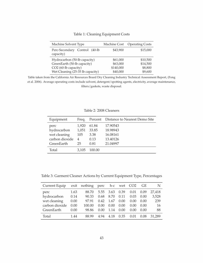
Table 1: Cleaning Equipment Costs

Machine Solvent Type Machine Cost Operating Costs

Perc-Secondary Control (40-lbcapacity)

$43,900 $15,000

Hydrocarbon (50-lb capacity) $61,000 $10,500GreenEarth (50-lb capacity) $63,000 $14,500CO2 (60-lb capacity) $140,000 $8,800Wet Cleaning (25-35 lb capacity) $40,000 $9,600

Table taken from the California Air Resources Board Dry Cleaning Industry Technical Assessment Report, (Fonget al. 2006). Average operating costs include solvent, detergent/spotting agents, electricity, average maintenance,

filters/gaskets, waste disposal.

Table 2: 2008 Cleaners

Equipment Freq. Percent Distance to Nearest Demo Site

perc 1,920 61.84 17.90543hydrocarbon 1,051 33.85 18.98943wet cleaning 105 3.38 16.08161carbon dioxide 4 0.13 13.40126GreenEarth 25 0.81 21.04997

Total 3,105 100.00

Table 3: Garment Cleaner Actions by Current Equipment Type, Percentages

Current Equip exit nothing perc h-c wet CO2 GE N

perc 1.63 88.70 5.55 3.63 0.39 0.01 0.09 27,418hydrocarbon 0.14 90.33 0.68 8.70 0.11 0.03 0.00 3,528wet cleaning 0.00 97.91 0.42 1.67 0.00 0.00 0.00 239carbon dioxide 0.00 100.00 0.00 0.00 0.00 0.00 0.00 16GreenEarth 0.00 98.86 0.00 1.14 0.00 0.00 0.00 88

Total 1.44 88.99 4.94 4.18 0.35 0.01 0.08 31,289

43

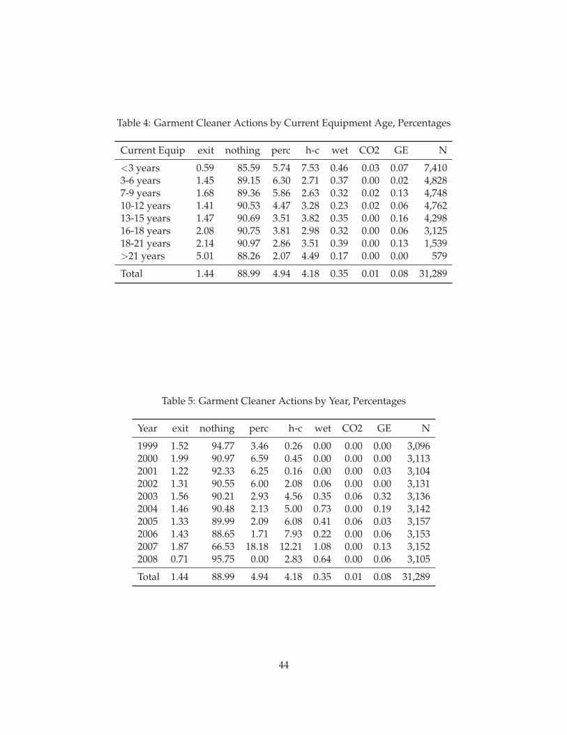
Table 4: Garment Cleaner Actions by Current Equipment Age, Percentages

Current Equip exit nothing perc h-c wet CO2 GE N

<3 years 0.59 85.59 5.74 7.53 0.46 0.03 0.07 7,4103-6 years 1.45 89.15 6.30 2.71 0.37 0.00 0.02 4,8287-9 years 1.68 89.36 5.86 2.63 0.32 0.02 0.13 4,74810-12 years 1.41 90.53 4.47 3.28 0.23 0.02 0.06 4,76213-15 years 1.47 90.69 3.51 3.82 0.35 0.00 0.16 4,29816-18 years 2.08 90.75 3.81 2.98 0.32 0.00 0.06 3,12518-21 years 2.14 90.97 2.86 3.51 0.39 0.00 0.13 1,539>21 years 5.01 88.26 2.07 4.49 0.17 0.00 0.00 579

Total 1.44 88.99 4.94 4.18 0.35 0.01 0.08 31,289

Table 5: Garment Cleaner Actions by Year, Percentages

Year exit nothing perc h-c wet CO2 GE N

1999 1.52 94.77 3.46 0.26 0.00 0.00 0.00 3,0962000 1.99 90.97 6.59 0.45 0.00 0.00 0.00 3,1132001 1.22 92.33 6.25 0.16 0.00 0.00 0.03 3,1042002 1.31 90.55 6.00 2.08 0.06 0.00 0.00 3,1312003 1.56 90.21 2.93 4.56 0.35 0.06 0.32 3,1362004 1.46 90.48 2.13 5.00 0.73 0.00 0.19 3,1422005 1.33 89.99 2.09 6.08 0.41 0.06 0.03 3,1572006 1.43 88.65 1.71 7.93 0.22 0.00 0.06 3,1532007 1.87 66.53 18.18 12.21 1.08 0.00 0.13 3,1522008 0.71 95.75 0.00 2.83 0.64 0.00 0.06 3,105

Total 1.44 88.99 4.94 4.18 0.35 0.01 0.08 31,289

44

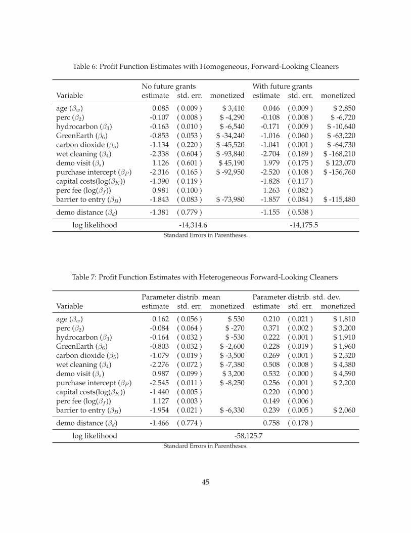
Table 6: Profit Function Estimates with Homogeneous, Forward-Looking Cleaners

No future grants With future grantsVariable estimate std. err. monetized estimate std. err. monetized

age (βw) 0.085 ( 0.009 ) $ 3,410 0.046 ( 0.009 ) $ 2,850perc (β2) -0.107 ( 0.008 ) $ -4,290 -0.108 ( 0.008 ) $ -6,720hydrocarbon (β3) -0.163 ( 0.010 ) $ -6,540 -0.171 ( 0.009 ) $ -10,640GreenEarth (β6) -0.853 ( 0.053 ) $ -34,240 -1.016 ( 0.060 ) $ -63,220carbon dioxide (β5) -1.134 ( 0.220 ) $ -45,520 -1.041 ( 0.001 ) $ -64,730wet cleaning (β4) -2.338 ( 0.604 ) $ -93,840 -2.704 ( 0.189 ) $ -168,210demo visit (βs) 1.126 ( 0.601 ) $ 45,190 1.979 ( 0.175 ) $ 123,070purchase intercept (βP ) -2.316 ( 0.165 ) $ -92,950 -2.520 ( 0.108 ) $ -156,760capital costs(log(βK)) -1.390 ( 0.119 ) -1.828 ( 0.117 )perc fee (log(βf )) 0.981 ( 0.100 ) 1.263 ( 0.082 )barrier to entry (βB) -1.843 ( 0.083 ) $ -73,980 -1.857 ( 0.084 ) $ -115,480

demo distance (βd) -1.381 ( 0.779 ) -1.155 ( 0.538 )

log likelihood -14,314.6 -14,175.5Standard Errors in Parentheses.

Table 7: Profit Function Estimates with Heterogeneous Forward-Looking Cleaners

Parameter distrib. mean Parameter distrib. std. dev.Variable estimate std. err. monetized estimate std. err. monetized

age (βw) 0.162 ( 0.056 ) $ 530 0.210 ( 0.021 ) $ 1,810perc (β2) -0.084 ( 0.064 ) $ -270 0.371 ( 0.002 ) $ 3,200hydrocarbon (β3) -0.164 ( 0.032 ) $ -530 0.222 ( 0.001 ) $ 1,910GreenEarth (β6) -0.803 ( 0.032 ) $ -2,600 0.228 ( 0.019 ) $ 1,960carbon dioxide (β5) -1.079 ( 0.019 ) $ -3,500 0.269 ( 0.001 ) $ 2,320wet cleaning (β4) -2.276 ( 0.072 ) $ -7,380 0.508 ( 0.008 ) $ 4,380demo visit (βs) 0.987 ( 0.099 ) $ 3,200 0.532 ( 0.000 ) $ 4,590purchase intercept (βP ) -2.545 ( 0.011 ) $ -8,250 0.256 ( 0.001 ) $ 2,200capital costs(log(βK)) -1.440 ( 0.005 ) 0.220 ( 0.000 )perc fee (log(βf )) 1.127 ( 0.003 ) 0.149 ( 0.006 )barrier to entry (βB) -1.954 ( 0.021 ) $ -6,330 0.239 ( 0.005 ) $ 2,060

demo distance (βd) -1.466 ( 0.774 ) 0.758 ( 0.178 )

log likelihood -58,125.7Standard Errors in Parentheses.

45

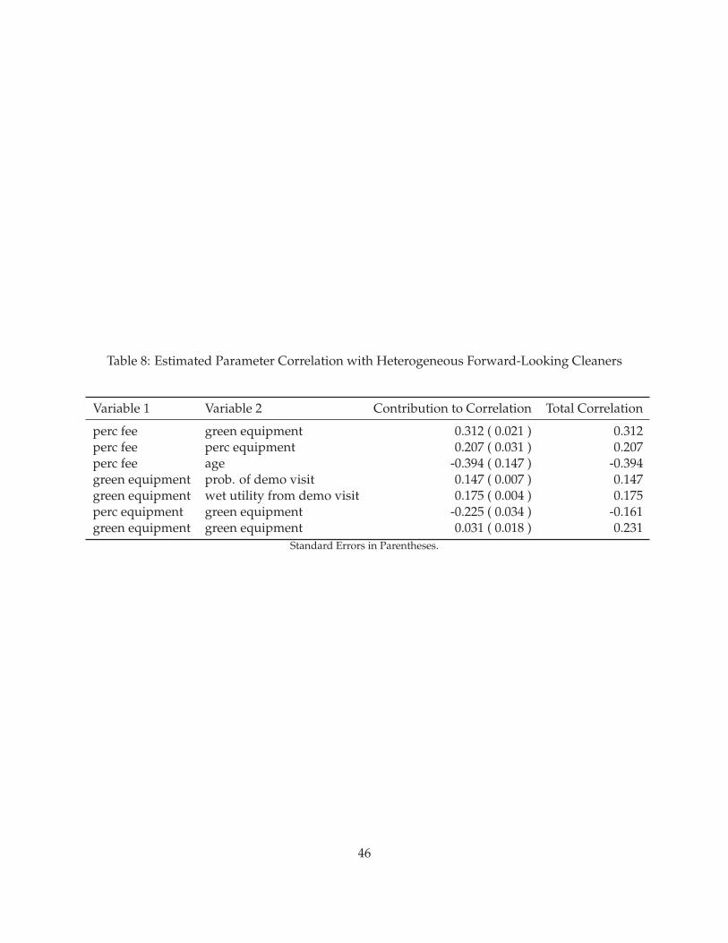
Table 8: Estimated Parameter Correlation with Heterogeneous Forward-Looking Cleaners

Variable 1 Variable 2 Contribution to Correlation Total Correlation

perc fee green equipment 0.312 ( 0.021 ) 0.312perc fee perc equipment 0.207 ( 0.031 ) 0.207perc fee age -0.394 ( 0.147 ) -0.394green equipment prob. of demo visit 0.147 ( 0.007 ) 0.147green equipment wet utility from demo visit 0.175 ( 0.004 ) 0.175perc equipment green equipment -0.225 ( 0.034 ) -0.161green equipment green equipment 0.031 ( 0.018 ) 0.231

Standard Errors in Parentheses.

46

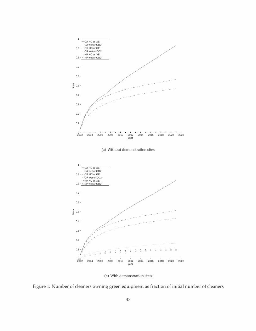
2002 2004 2006 2008 2010 2012 2014 2016 2018 2020 20220

0.1

0.2

0.3

0.4

0.5

0.6

0.7

0.8

0.9

1

year

firm

s

CA HC or GECA wet or CO2OR HC or GEOR wet or CO2NP HC or GENP wet or CO2

(a) Without demonstration sites

2002 2004 2006 2008 2010 2012 2014 2016 2018 2020 20220

0.1

0.2

0.3

0.4

0.5

0.6

0.7

0.8

0.9

1

year

firm

s

CA HC or GECA wet or CO2OR HC or GEOR wet or CO2NP HC or GENP wet or CO2

(b) With demonstration sites

Figure 1: Number of cleaners owning green equipment as fraction of initial number of cleaners

47

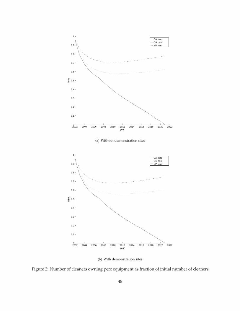
2002 2004 2006 2008 2010 2012 2014 2016 2018 2020 20220

0.1

0.2

0.3

0.4

0.5

0.6

0.7

0.8

0.9

1

year

firm

s

CA percOR percNP perc

(a) Without demonstration sites

2002 2004 2006 2008 2010 2012 2014 2016 2018 2020 20220

0.1

0.2

0.3

0.4

0.5

0.6

0.7

0.8

0.9

1

year

firm

s

CA percOR percNP perc

(b) With demonstration sites

Figure 2: Number of cleaners owning perc equipment as fraction of initial number of cleaners

48

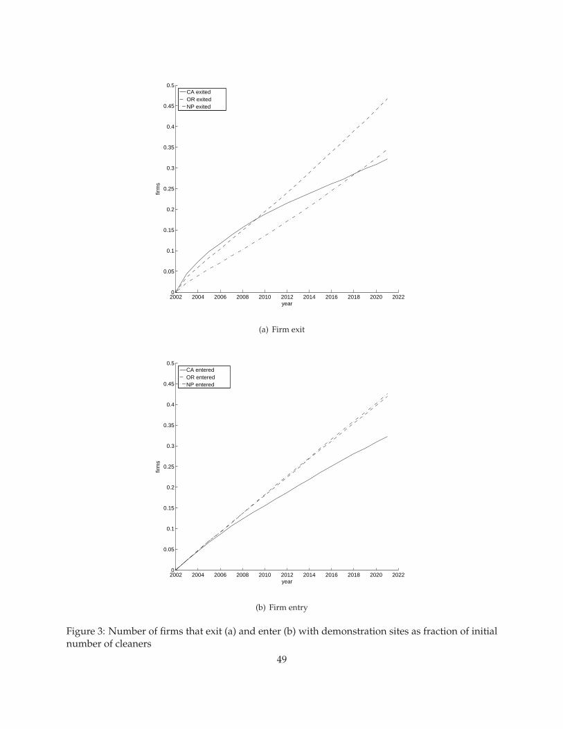
2002 2004 2006 2008 2010 2012 2014 2016 2018 2020 20220

0.05

0.1

0.15

0.2

0.25

0.3

0.35

0.4

0.45

0.5

year

firm

s

CA exitedOR exitedNP exited

(a) Firm exit

2002 2004 2006 2008 2010 2012 2014 2016 2018 2020 20220

0.05

0.1

0.15

0.2

0.25

0.3

0.35

0.4

0.45

0.5

year

firm

s

CA enteredOR enteredNP entered

(b) Firm entry

Figure 3: Number of firms that exit (a) and enter (b) with demonstration sites as fraction of initialnumber of cleaners

49

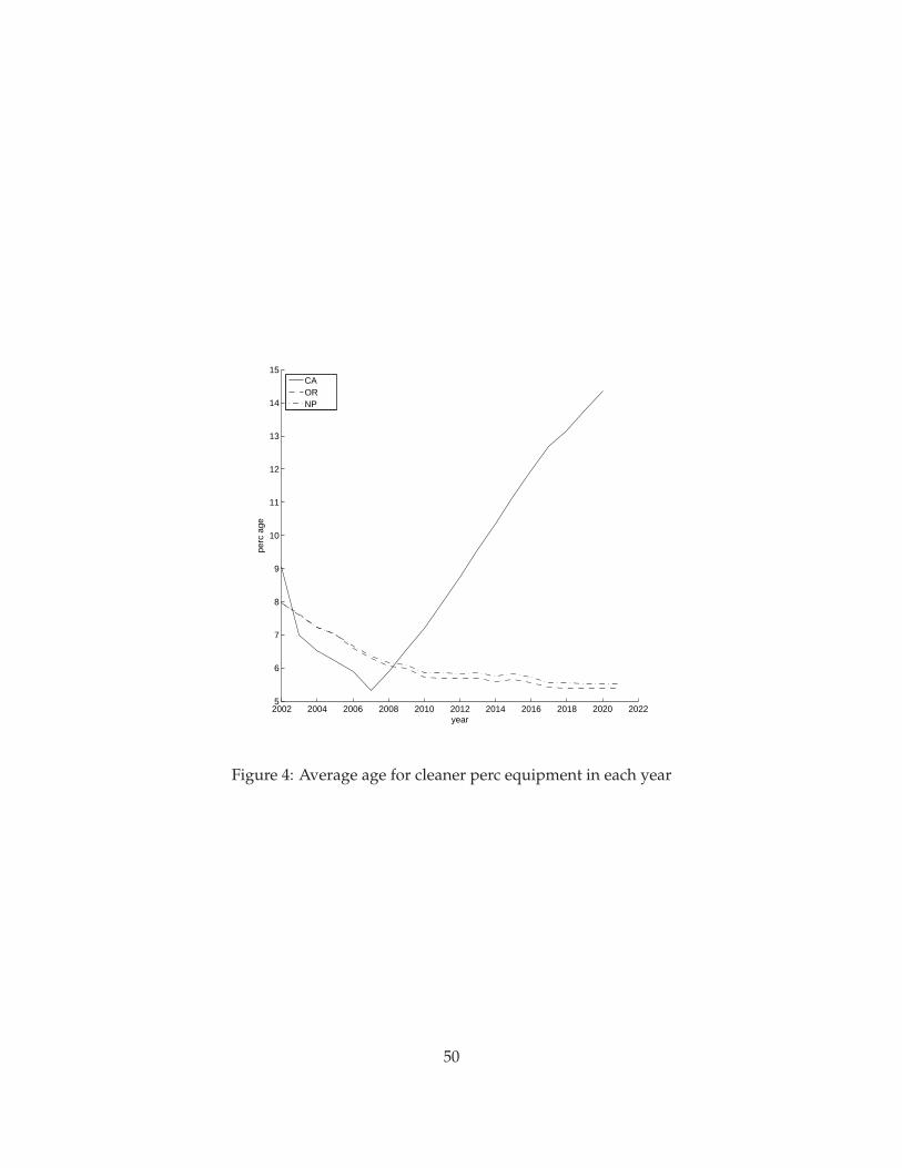
2002 2004 2006 2008 2010 2012 2014 2016 2018 2020 20225

6

7

8

9

10

11

12

13

14

15

year

perc

age

CAORNP

Figure 4: Average age for cleaner perc equipment in each year

50