Embed Size (px)
Citation preview
Master of Science ThesisStockholm, Sweden 2013
TRITA-ICT-EX-2013:97
D A V I D P E I N A D O G U T I E R R E Z
Green DAS
Green Distributed Antenna Systems
K T H I n f o r m a t i o n a n d
C o m m u n i c a t i o n T e c h n o l o g y

ii
iii
Green Distributed Antenna System (Green DAS)
David Peinado Gutiérrez
Master Thesis in Information and Communication Technology,
June 2013
Examiner: Anders Västberg
Internal Advisor: Mats Nilson
External Advisors: Mikhail Popov (Acreo AB)
Tord Sjölund (Mic Nordic AB)

iv
KTH, School of Information and Communications Technology (ICT)
Department of Communication Systems (COS)
© David Peinado Gutiérrez, May 2013
v
Abstract
Energy saving is an important factor which must be taken into account when planning a
mobile distribution network.
Distributed Antenna System (DAS) is a part of mobile distribution infrastructure which
is used to extend the coverage of mobile base stations. DAS is a subject of the present
study whose goal is to optimize DAS solutions for indoor and outdoor scenarios in
terms of energy consumption while preserving the required Quality-of-Service (QoS).
The project outdoor scenario is built on an example of a football stadium (Friends Arena
in Stockholm) and the indoor scenario on an example of an office building (Electrum).
The propagation model is build under realistic assumptions. The energy efficiency is
defined as Joule/bit.
Taking into account the radio part only, it is shown that increasing the number of
antennas allows to improve the energy efficiency. It is also shown that by adjusting the
positions of the antennas using an optimization algorithm, one can further improve the
energy efficiency. It is finally shown that taking into account both radio and optical
parts, there is an upper bound for the energy efficiency (as a function of the number of
antennas), i.e. there is generally an optimal number of antennas which provide the best
energy efficiency with a fixed QoS for the system.
This thesis is a part of the joint project “Green Distributed Antenna Systems” between
Wireless@KTH, Acreo AB and MIC Nordic AB

vi
Acknowledgments
First of all I would like to express my gratitude to my internal advisors Anders Västberg
and Mats Nilson for helping me with the technical questions and for making my
adaptation to the pace work in the Wireless@KTH department become more easy and
more comfortable in these fantastic facilities.
I also would like to thank each and every one of those who were present at some time in
the many meetings held during the semester, for providing their valuable knowledge
and good advices. Special mention to Tord Sjölund, is pleasing to see that a
businessman attend meetings in order to contribute and collaborate on the project.
But if there is anyone who deserves special thanks, that is Mikhail Popov. I would like
to thank him for his continued support, for helping me in each and every one of the
times that I needed and for teaching me how is the day to day on the tight world of real
work. I also think that some meetings have never been as productive as ours. “Gracias
amigo”.
Last but not least, of course, I would like to mention my family, especially my parents
Rafael and Aurelia, my brother Víctor and my girlfriend Núria, who have been a
continuous and unconditional support during my career in general and, particularly, this
year despite the distance that has separated us.
vii
Contents:
Abstract ............................................................................................................. v
Acknowledgments ........................................................................................... vi
List of Figures ................................................................................................... x
List of Tables ................................................................................................. xiii
Chapter 1 Introduction ............................ ......................................................... 1
1.1 Background ....................................................................................................... 1
1.2 Thesis Motivation .............................................................................................. 2
1.3 Problem Formulation ......................................................................................... 2
1.4 Report Outline ................................................................................................... 2
Chapter 2 Introduction to DAS ..................... ................................................... 4
2.1 Distributed Antenna System Solutions ............................................................... 4
2.2 Passive Distributed Antenna System ................................................................. 4
2.2.1 Passive DAS Architecture ...................................................................... 4
2.3 Active Distributed Antenna System .................................................................... 6
2.3.1 Active DAS Architecture ......................................................................... 6
2.4 DAS Architecture studied in the thesis ............................................................... 8
Chapter 3 DAS System Modeling ..................... ............................................. 10
3.1 Component Characteristics ............................................................................. 10
3.2 Link Budget ..................................................................................................... 10
viii
3.2.1 Components in the Link Budget ........................................................... 11
3.2.2 The Path Loss Model ........................................................................... 14
3.3 Signal to Noise Ratio ....................................................................................... 16
3.3.1 Interference Behavior ........................................................................... 17
3.4 Channel Capacity ............................................................................................ 17
3.5 Energy Efficiency Factor .................................................................................. 17
3.6 Overview of UMTS .......................................................................................... 18
Chapter 4 Scenario Modeling ....................... ................................................. 20
4.1 Outdoor Case .................................................................................................. 20
4.2 Indoor Case ..................................................................................................... 22
Chapter 5 Simulation .............................. ....................................................... 24
5.1 About MATLAB® .............................................................................................. 24
5.2 Simulation Process .......................................................................................... 24
5.2.1 Scenarios and Observation Points ....................................................... 25
5.2.2 Antenna Positions ................................................................................ 26
5.2.3 Calculation of QoS Parameters ............................................................ 27
5.2.4 Phase Diagram .................................................................................... 27
Chapter 6 Optimization ............................ ...................................................... 29
6.1 Overview of Genetic Algorithm ........................................................................ 29
6.2 Optimization Process ....................................................................................... 30
6.2.1 Parameters Involved ............................................................................ 30
6.2.2 Cost Function ....................................................................................... 31
6.2.3 Applying Genetic Algorithm .................................................................. 32
Chapter 7 Showcases and Results ................... ............................................ 34
ix
7.1 Required Quality of Service ............................................................................. 34
7.2 Showcases Description ................................................................................... 34
7.2.1 Efficiency Trends Case ........................................................................ 34
7.2.2 Optimization Case ................................................................................ 34
7.2.3 Optical-Wireless Case .......................................................................... 35
7.3 Simulations ...................................................................................................... 35
7.3.1 Efficiency Trends Case ........................................................................ 35
7.3.1.1 Results ..................................................................................... 49
7.3.1.2 Conclusion on the results .......................................................... 50
7.3.2 Optimization Case ................................................................................ 51
7.3.2.1 Outdoor Case ........................................................................... 51
7.3.2.2 Results ..................................................................................... 61
7.3.2.3 Conclusion on the results .......................................................... 62
7.3.2.4 Indoor Case Results ................................................................. 62
7.3.2.5 Interference Study Results ........................................................ 65
7.3.2.6 Conclusion on the results .......................................................... 67
7.3.3 Optical-Wireless Case .......................................................................... 69
7.3.3.1 Conclusion on the results .......................................................... 73
Chapter 8 Conclusion and Future Work .............. ......................................... 76
References ........................................ .............................................................. 78
x
List of Figures Figure 2.1 Typical indoor Passive DAS architecture
Figure 2.2 Typical active dual band DAS architecture
Figure 3.1 Isotropic ideal radiation patterns
Figure 3.2 180o directive ideal radiation patterns
Figure 3.3 90o directive ideal radiation patterns
Figure 3.4 Even coax power splitters
Figure 3.5 Taps, adjustable and fixed
Figure 3.6 Example of a path loss slope, based on measurement samples
Figure 3.7 Distance between two points in a 3D plane
Figure 3.8 FDMA, TDMA and CDMA schemes
Figure 3.9 UMTS UL and DL frequencies distribution
Figure 3.10 UMTS codes distribution
Figure 4.1 View of the Stadium #1
Figure 4.2 View of the Stadium #2 with omnidirectional antennas
Figure 4.3 View of the 2 floors building
Figure 4.4 Distribution at indoor building
Figure 5.1 Components distribution in each simulation
Figure 5.2 Indoor scenario model and distribution of observation points
Figure 5.3 Outdoor scenario model and distribution of observation points
Figure 5.4 Block Diagram of Simulation Process
Figure 6.1 One-point & N-point crossover operators
Figure 6.2 Chromosome Composition
Figure 6.3 Optimization Phases Diagram
Figure 7.1.1 One Antenna Scenario
Figure 7.1.2 SNR Measured with One Antenna
Figure 7.1.3 Capacity Measured with One Antenna
Figure 7.1.4 Two Antennas Scenario
Figure 7.1.5 Capacity with Two Omnidirectional Antennas neglecting LCOAX
Figure 7.1.6 Capacity with Two Omnidirectional Antennas considering LCOAX
Figure 7.1.7 Capacity with Two 180º Directive Antennas neglecting LCOAX
Figure 7.1.8 Capacity with Two 180º Directive Antennas considering LCOAX
xi
Figure 7.1.9 Four Antennas Scenario
Figure 7.1.10 SNR with Four Omnidirectional Antennas neglecting LCOAX
Figure 7.1.11 Capacity with Four Omnidirectional Antennas neglecting LCOAX
Figure 7.1.12 SNR with Four Omnidirectional Antennas considering LCOAX
Figure 7.1.13 Capacity with Four Omnidirectional Antennas considering LCOAX
Figure 7.1.14 SNR with Four 180º Directive Antennas neglecting LCOAX
Figure 7.1.15 Capacity with Four 180º Directive Antennas neglecting LCOAX
Figure 7.1.16 SNR with Four 180º Directive Antennas considering LCOAX
Figure 7.1.17 Capacity with Four 180º Directive Antennas considering LCOAX
Figure 7.1.18 Four Antennas in the corners Scenario
Figure 7.1.19 SNR with Four 90º Directive Antennas neglecting LCOAX
Figure 7.1.20 Capacity with Four 90º Directive Antennas neglecting LCOAX
Figure 7.1.21 SNR with Four 90º Directive Antennas considering LCOAX
Figure 7.1.22 Capacity with Four 90º Directive Antennas considering LCOAX
Figure 7.1.23 Power values graph when neglecting coax losses
Figure 7.1.24 Power values graph when considering coax losses
Figure 7.2.1 SNR with Antennas in the corners neglecting LCOAX
Figure 7.2.2 Capacity with Antennas in the corners neglecting LCOAX
Figure 7.2.3 Optimal Positions of Antennas when neglecting LCOAX
Figure 7.2.4 Evolution of the Cost Function in the Optimization Process
Figure 7.2.5 SNR with Antennas in the corners considering LCOAX
Figure 7.2.6 Capacity with Antennas in the corners considering LCOAX
Figure 7.2.7 Optimal Positions of Antennas when considering LCOAX
Figure 7.2.8 SNR with Antennas in optimal positions considering LCOAX
Figure 7.2.9 Capacity with Antennas in optimal positions considering LCOAX
Figure 7.2.10 Capacity with Antennas in the corners neglecting LCOAX
Figure 7.2.11 Optimal Positions of Antennas when neglecting LCOAX
Figure 7.2.12 Evolution of the Cost Function in the Optimization Process
Figure 7.2.13 Capacity with Antennas in optimal positions neglecting LCOAX
Figure 7.2.14 Capacity with Antennas in the corners considering LCOAX
Figure 7.2.15 Optimal Positions of Antennas when considering LCOAX
Figure 7.2.16 Evolution of the Cost Function in the Optimization Process
Figure 7.2.17 Capacity with Antennas in optimal positions considering LCOAX
xii
Figure 7.2.18 Capacity with Antennas in the corners
Figure 7.2.19 Optimal Positions of Antennas for Indoor case
Figure 7.2.20 Evolution of the Cost Function in the Optimization Process
Figure 7.2.21 Capacity with Antennas in the optimal positions
Figure 7.2.22 Capacity neglecting the interferences effect from the second floor
Figure 7.2.23 Capacity considering the interferences effect from the second floor
Figure 7.3.1 Capacity levels with 1 Antenna-RU
Figure 7.3.2 Capacity levels with 2 Antenna-RU
Figure 7.3.3 Capacity levels with 4 Antenna-RU
Figure 7.3.4 Scenario with the distribution of 6 Antennas-RU
Figure 7.3.5 Capacity levels with 6 Antenna-RU
Figure 7.3.6 Scenario with the distribution of 8 Antenna-RU
Figure 7.3.7 Capacity levels with 8 Antenna-RU
Figure 7.3.8 Total Power consumption VS Number of Antennas (I)
Figure 7.3.9 Total Power consumption VS Number of Antennas (II)
Figure 7.3.10 Total Power consumption VS Number of Antennas (III)

xiii
List of Tables
Table 3.1 Typical attenuation of coaxial cable
Table 3.2 PLS constants for different environments
Table 3.3 Free Space Losses at 1 m for different frequencies
Table 4.1 Wall losses at different operating frequencies
Table 7.1 Required Power in each case
Table 7.2 Values of Powers and Energy Savings in Optimization Case (I)
Table 7.3 Values of Powers and Energy Savings in Optimization Case (II)
Table 7.4 Values of Capacity and required Powers in indoor case
Table 7.5 Values of Capacity with and without interferences
Table 7.6 Total Power Consumption (I)
Table 7.7 Total Power Consumption (II)
Table 7.8 Total Power Consumption (III)
1
Chapter 1 Introduction 1.1 Background
Thanks to the implacable development of the communication sector, it is allowed to
establish connections in ways that were unthinkable only 20 years ago.
In 1982, during the European Conference of Postal and Telecommunications
Administrations (CEPT), 26 European companies of telecommunications created the
GSM (Group Special Mobile) group, whose tasks were to develop a European standard
for digital cellular voice telephony [1].
In 1990 and 1991, there were created the standards GSM-900 and DCS-1800
respectively. Nowadays, GSM is the most extended standard all over the world with
more than the 80 % of the mobile terminals in use. It has about 3000 million users in
212 different countries, being the predominant standard in Europe, South America, Asia
and Oceania besides having a huge extension in North America [1].
Encompassing the GSM system as 2G (second generation) system, it was during the
first years of the 21st century when the 3G made its appearance. This new
communication standard allows the transmission of voice and data over the mobile
telephony through the UMTS (Universal Mobile Telecommunications System).
Improving the GSM features, this standard allows introducing more users into the
global network of the system and increases the speed up to 2 Mbps per user. UMTS
combines GSM with more efficient bandwidth and uses CDMA (Code Division
Multiple Access) architecture. Because of that, it was possible to move from the original
rate of 9.6 Kbps to rates that are close to 14 Mbps in one of the latest evolution provided
by UMTS, HSPDA (High-Speed Downlink Packet Access). Currently the HSPA+
technology is available providing speeds of up to 84 Mbps in downlink and 22 Mbps in
uplink [2].
With such advances in rates, to provide a service with a certain minimum of quality to
as many users as possible has become challenging for the operators when planning their
networks. Demand of service from users keeps growing and it is clear that the radio
network capacity has to increase.
2
There are implemented already solutions that allow to improve the quality of service in
terms of capacity and coverage. The most common solutions consist on include
additional frequency carriers, add/increase the sectorization or use signal-repeaters [3].
However, these solutions are far from being the optimal ones in terms of energy saving
due to the corresponding high power consumption. The implementation of DAS will
offer improvements in terms of energy efficiency and provided QoS. [4, 5].
By studying the features of distributed antennas and with analytic methods of
calculation and optimization, we will be guided to find the optimal solution that achieve
an energy saving retaining the quality of service of the system.
1.2 Thesis Motivation DAS (Distributed Antenna System) are used to improve the coverage of a single or
multiple base stations by using a distributed infrastructure of remote antenna connected
to the base station or base stations (2G, 3G or LTE) via fibers or coaxial cables [4].
So far, the architecture, planning and deployment of DAS do not take the energy
consumption into consideration. It is still an open general question on how the
architecture and other parameters of F-DAS (Fiber-based DAS) can affect its total
energy consumption [6].
An important aspect is that a re-designed architecture can provide the required quality
of service (QoS) over a defined area with better energy use than the original planning.
1.3 Problem Formulation The actual scope of the thesis is to investigate the energy efficient DAS and its main
components with the goal to optimize the energy consumption in the radio access
segment of mobile communication networks.
The thesis answers the following questions:
• Is the energy saving possible retaining the quality of service?
• Can the signal-to-noise-ratio, and respectively channel capacity that the system
is able to provide, be improved without increasing the supplied power by the
base station?
3
• Given that the environment is known, what is the optimal balance between the
number of nodes and their power to provide a defined QoS?
• How do the different components of the system affect when planning the
architecture?
1.4 Report Outline
Chapter #2: An introduction to Distribute Antenna System architectures: typical
solutions that are implemented in indoor and outdoor cases. The design
of the studied DAS is presented providing also the pros and cons of the
passive and active architectures
.
Chapter #3: Explanation of how all the components from MU (Master Unit) till the
antenna work. Which parameters are taken into account in the link
budget calculation and related formulas and the used methods (SNR,
path losses model) in the project are explained.
Chapter #4: Two real-life scenarios are presented. This chapter covers how the
scenarios have been modeled and the approximations that have been
done in order to create the models that allow us to work within the
simulation software.
Chapter #5: Information about how the simulations have been done. Detailed
processes and explanation of how the used MATLAB functions work
are covered in this chapter.
Chapter #6: Explanation of how the global optimization method works and how it
can help to achieve the goal in the thesis. One optimization method, the
Genetic Algorithm in particular, is detailed.
Chapter #7: Results before and after the simulations and optimization processes in
terms of power consumption and energy saving.
Chapter #8: Conclusion: what goals have been achieved and possible future work
lines in the area.
4
Chapter 2 Introduction to DAS 2.1 Distributed Antenna System Solutions
There are different possibilities of how a system with a certain uniform coverage level
can be designed. During this work are studied the passive distribution, the active
distribution and the hybrid solutions [2]. Each of these DAS has their pros and cons,
depending on the corresponding environment where they work and the required quality
of service.
Normally it is chosen the solution that offers a good balance between the most downlink
signal power at the outputs of the antennas, the least noise measured in the entire link
and the most uniform coverage provided by the entire system. Other parameters such as
power consumption and costs are taken into account when deciding the optimal
implementation [2, 4]. Furthermore, in particular for the project, one of the most
important parameter that will be taken into consideration will be the energy saving
factor that can be achieved.
2.2 Passive Distributed Antenna System The passive DAS is typically used for indoor scenarios such as small buildings. One of
the best advantages is that they are relatively easy to plan and install. The principal
requirement to comply when planning an indoor DAS is to know the maximum loss
than can be accumulated until the antennas in order to ensure that the system will
provide the required power, even in the worst conditions case. Typically, the passive
DAS consists of passive components such as coax cables, splitters, attenuators, couplers
or circulators [2].
2.2.1 Passive DAS Architecture
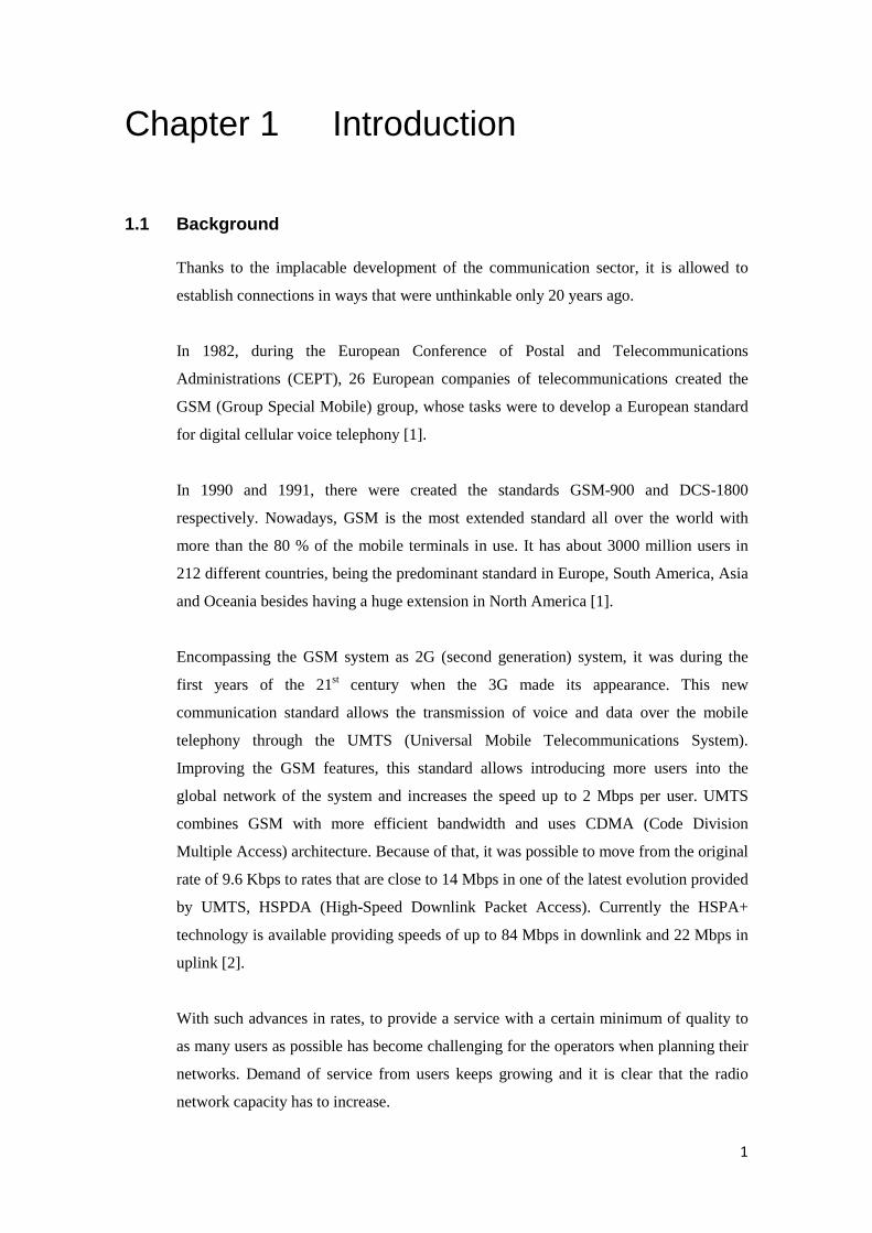
These kinds of systems are provided of a micro or macro high power base
station that feeds all the distributed antennas via the coaxial cables.
Obviously the coax cable will attenuate the signal from the base station till
the antenna depending on its thickness and the operating frequency. The
filters are responsible for selecting one frequency or another.
5
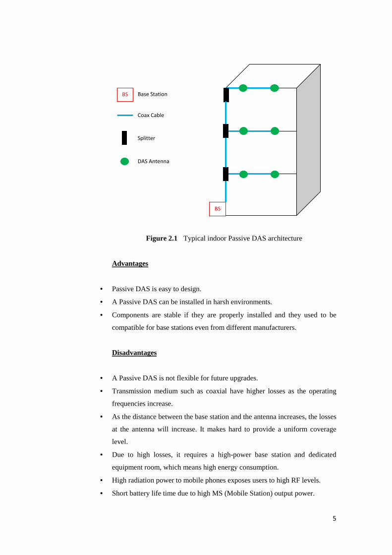
Figure 2.1 Typical indoor Passive DAS architecture
Advantages
• Passive DAS is easy to design.
• A Passive DAS can be installed in harsh environments.
• Components are stable if they are properly installed and they used to be
compatible for base stations even from different manufacturers.
Disadvantages
• A Passive DAS is not flexible for future upgrades.
• Transmission medium such as coaxial have higher losses as the operating
frequencies increase.
• As the distance between the base station and the antenna increases, the losses
at the antenna will increase. It makes hard to provide a uniform coverage
level.
• Due to high losses, it requires a high-power base station and dedicated
equipment room, which means high energy consumption.
• High radiation power to mobile phones exposes users to high RF levels.
• Short battery life time due to high MS (Mobile Station) output power.
BS
BS Base Station
Coax Cable
Splitter
DAS Antenna
6
• It is hard to provide good service for 3G case in particular: high operating
frequencies and high data rates require better RF link requirements (low
losses and higher signal level).
2.3 Active Distributed Antenna System
There are differences in how an active distributed antenna system distributes the signal
to the antennas in comparison with the passive DAS. The active DAS normally relies on
optical fibers, making the installation work easier compared with the usually thick rigid
cables used for passive systems [4].
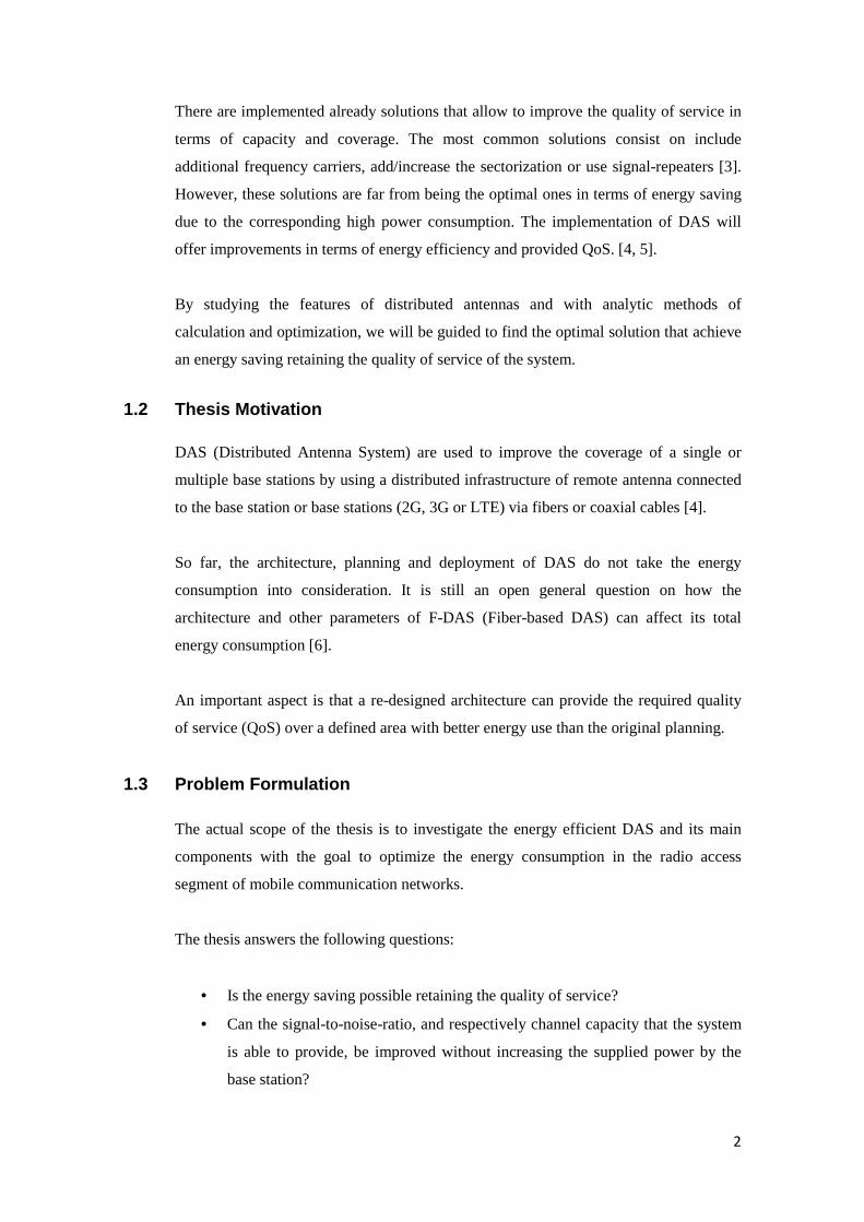
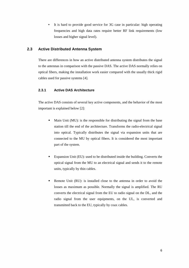
2.3.1 Active DAS Architecture
The active DAS consists of several key active components, and the behavior of the most
important is explained below [2]:
� Main Unit (MU): is the responsible for distributing the signal from the base
station till the end of the architecture. Transforms the radio-electrical signal
into optical. Typically distributes the signal via expansion units that are
connected to the MU by optical fibers. It is considered the most important
part of the system.
� Expansion Unit (EU): used to be distributed inside the building. Converts the
optical signal from the MU to an electrical signal and sends it to the remote
units, typically by thin cables.
� Remote Unit (RU): is installed close to the antenna in order to avoid the
losses as maximum as possible. Normally the signal is amplified. The RU
converts the electrical signal from the EU to radio signal on the DL, and the
radio signal from the user equipments, on the UL, is converted and
transmitted back to the EU, typically by coax cables.
7
Figure 2.2 Typical active dual band DAS architecture
Advantages
• The total losses in active DAS are lower than in the passive DAS.
• The signal power that feeds the DAS is the same that is measured at the
output of the antennas plus the gain of the system.
• Users experience less RF exposure levels when using active DAS as
compared to passive DAS. This is due to the fact that, active DAS use
optical fiber and active components, which compensates for the
transmission path loss.
• Active DAS provides a uniform coverage throughout the network: an
antenna at 2 meters away from the BS radiates the same signal level if the
same antenna is at 100 meters away from the BS (without taking into
consideration the effect of the RU in the signal power). This is due to no
perceived losses in the optical fibers.
• Active DAS needs less power from the base station. This is an important
point to take into consideration in terms of energy saving since the power
consumption is being reduced substantially.
Optical Fiber (Up to 6 km)
GSM
UMTS
MU
EU
EU
RU
RU
RU
RU
RU
RU
…
…
…
Thin cables (Up to 6 km) Coax Cable
Antennas
• Higher battery life time than in the passive DAS due to the lower MS output
power required.
• In active DAS
any degradation
there is no need to use excessive downlink power from the base stati
compensate for the losses.
Disadvantages
• An Active DAS is more difficult to design and sometimes results hard to
access to the components.
• More expensive equipment.
• Less compatibility between components.
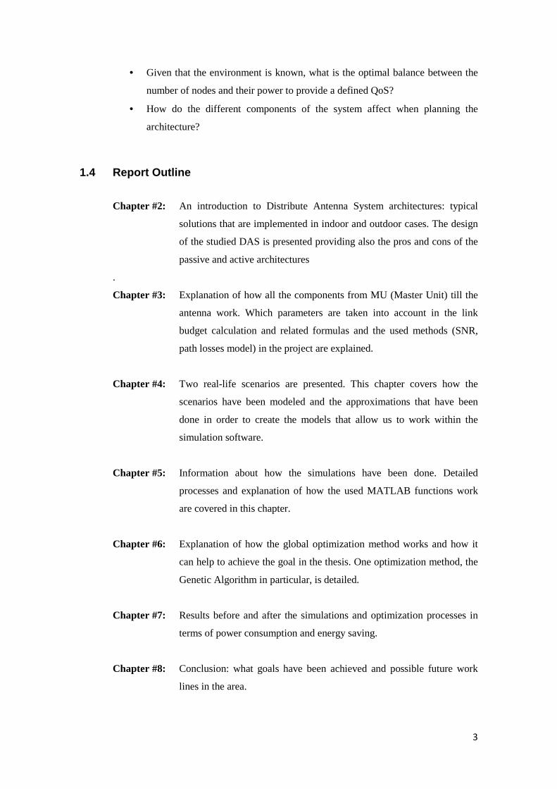
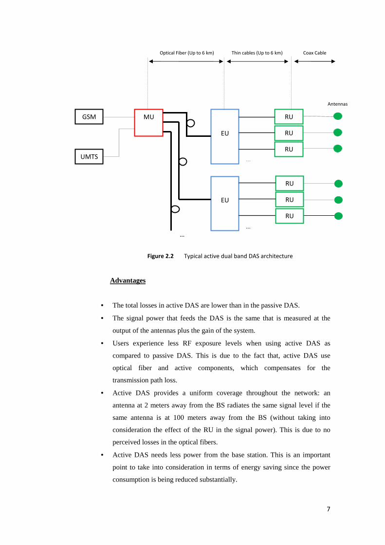
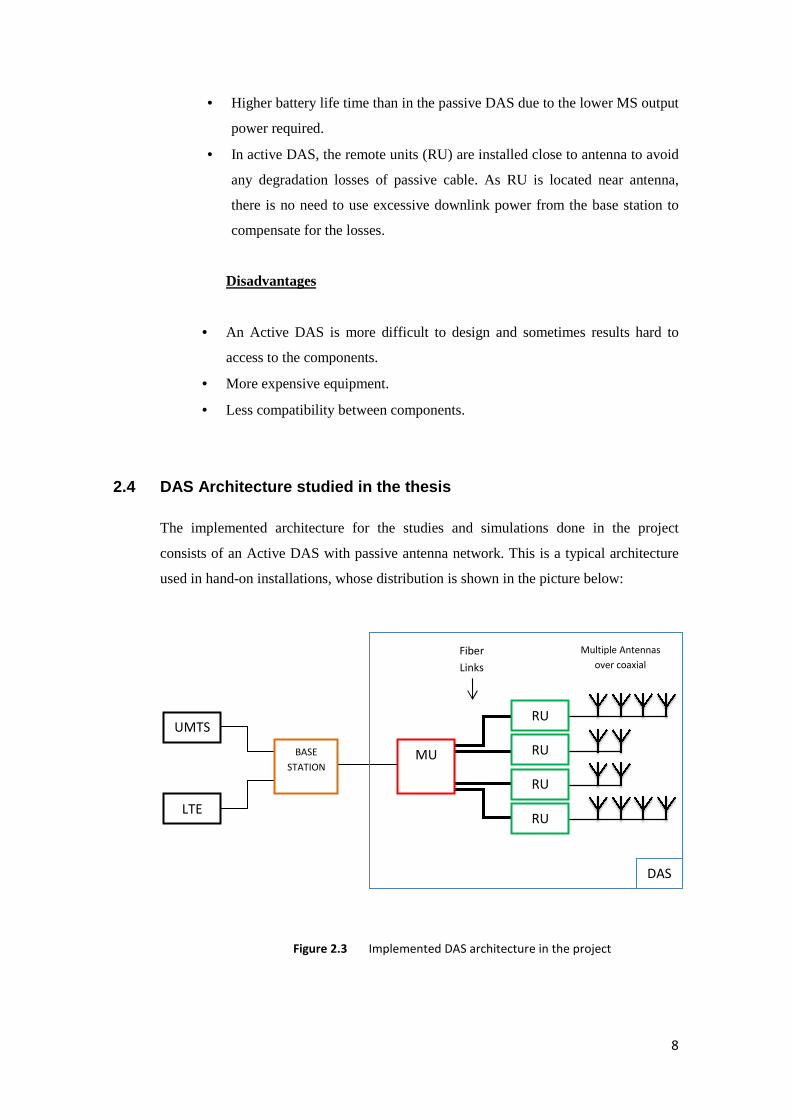
2.4 DAS Architecture The implemented architecture for the studies
consists of an Active D
used in hand-on installations,
UMTS
LTE
Higher battery life time than in the passive DAS due to the lower MS output
power required.
In active DAS, the remote units (RU) are installed close to antenna to avoid
any degradation losses of passive cable. As RU is located near antenna,
there is no need to use excessive downlink power from the base stati
compensate for the losses.
Disadvantages
An Active DAS is more difficult to design and sometimes results hard to
the components.
More expensive equipment.
Less compatibility between components.
DAS Architecture studied in the thesis
architecture for the studies and simulations done in the project
an Active DAS with passive antenna network. This is a typical architecture
on installations, whose distribution is shown in the picture below:
Figure 2.3 Implemented DAS architecture in the project
BASE
STATION MU
RU
RU
RU
RU
Fiber
Links
8
Higher battery life time than in the passive DAS due to the lower MS output
remote units (RU) are installed close to antenna to avoid
losses of passive cable. As RU is located near antenna,
there is no need to use excessive downlink power from the base station to
An Active DAS is more difficult to design and sometimes results hard to
done in the project
network. This is a typical architecture
whose distribution is shown in the picture below:
Implemented DAS architecture in the project
DAS
Multiple Antennas
over coaxial
9
The fiber links allow connecting the MU and the RU (in this case, there is no EU
between the MU and the RUs) without taking into consideration the losses in the coaxial
cable. By this way, it is possible to have an architecture where the MU and RU are
separated by long distances.
Since the wireless (or radio) part consists on a passive antenna network that are
interconnected by coax cable and splitters, one of the principal goals is to reduce the
loss effect that they have in the final power consumption results.
10
Chapter 3 DAS System Modeling 3.1 Component Characteristics
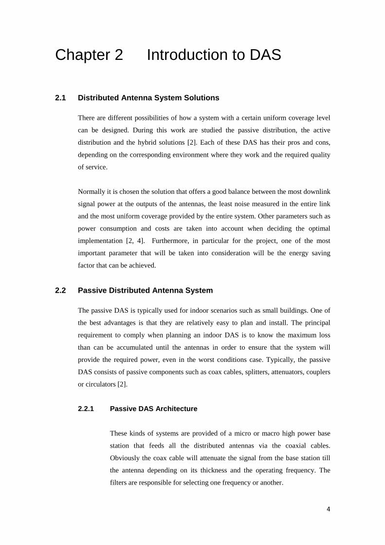
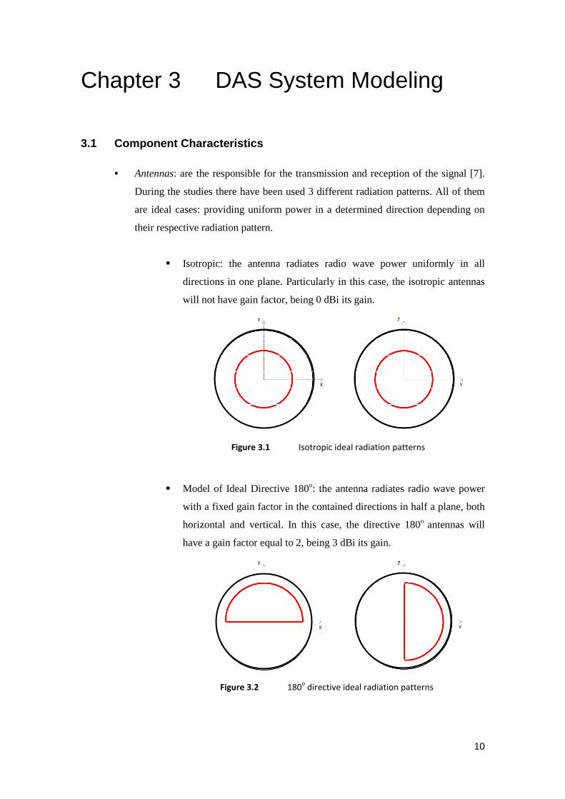
• Antennas: are the responsible for the transmission and reception of the signal [7].
During the studies there have been used 3 different radiation patterns. All of them
are ideal cases: providing uniform power in a determined direction depending on
their respective radiation pattern.
� Isotropic: the antenna radiates radio wave power uniformly in all
directions in one plane. Particularly in this case, the isotropic antennas
will not have gain factor, being 0 dBi its gain.
� Model of Ideal Directive 180o: the antenna radiates radio wave power
with a fixed gain factor in the contained directions in half a plane, both
horizontal and vertical. In this case, the directive 180o antennas will
have a gain factor equal to 2, being 3 dBi its gain.
Figure 3.1 Isotropic ideal radiation patterns
Figure 3.2 180o directive ideal radiation patterns
11
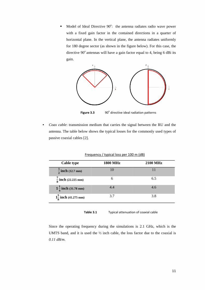
� Model of Ideal Directive 90o: the antenna radiates radio wave power
with a fixed gain factor in the contained directions in a quarter of
horizontal plane. In the vertical plane, the antenna radiates uniformly
for 180 degree sector (as shown in the figure below). For this case, the
directive 90o antennas will have a gain factor equal to 4, being 6 dBi its
gain.
• Coax cable: transmission medium that carries the signal between the RU and the
antenna. The table below shows the typical losses for the commonly used types of
passive coaxial cables [2].
Frequency / typical loss per 100 m (dB)
Cable type 1800 MHz 2100 MHz
��inch (12.7 mm) 10 11
�� inch (22.225 mm) 6 6.5
� �� inch (31.78 mm) 4.4 4.6
1�� inch (41.275 mm) 3.7 3.8
Table 3.1 Typical attenuation of coaxial cable
Since the operating frequency during the simulations is 2.1 GHz, which is the
UMTS band, and it is used the ½ inch cable, the loss factor due to the coaxial is
0.11 dB/m.
Figure 3.3 90o directive ideal radiation patterns
12
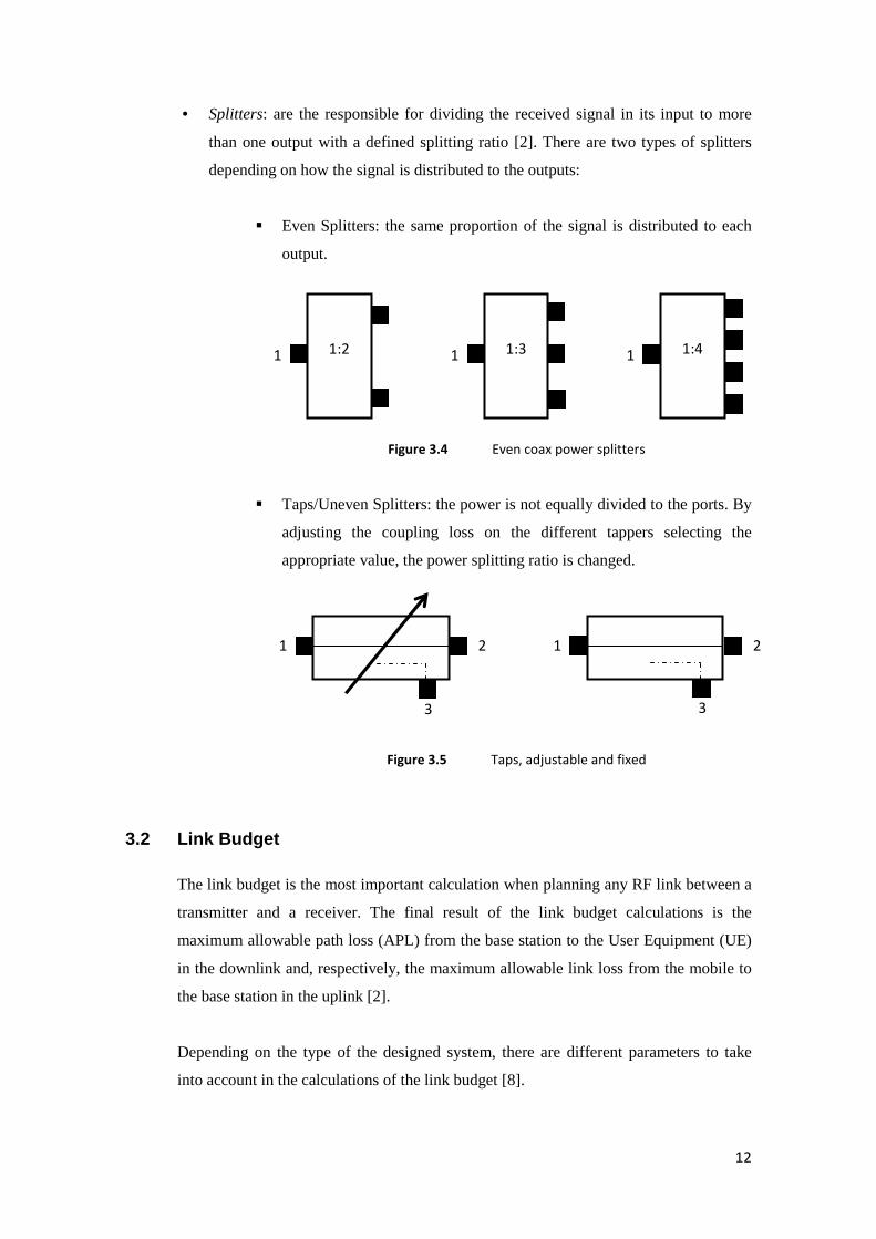
• Splitters: are the responsible for dividing the received signal in its input to more
than one output with a defined splitting ratio [2]. There are two types of splitters
depending on how the signal is distributed to the outputs:
� Even Splitters: the same proportion of the signal is distributed to each
output.
Figure 3.4 Even coax power splitters
� Taps/Uneven Splitters: the power is not equally divided to the ports. By
adjusting the coupling loss on the different tappers selecting the
appropriate value, the power splitting ratio is changed.
Figure 3.5 Taps, adjustable and fixed
3.2 Link Budget The link budget is the most important calculation when planning any RF link between a
transmitter and a receiver. The final result of the link budget calculations is the
maximum allowable path loss (APL) from the base station to the User Equipment (UE)
in the downlink and, respectively, the maximum allowable link loss from the mobile to
the base station in the uplink [2].
Depending on the type of the designed system, there are different parameters to take
into account in the calculations of the link budget [8].
1:3
1:2
1:4
1 2
3
1 2
3
1 1 1
13
3.2.1 Components in the Link Budget
The first parameter that is necessary to figure out in order to calculate the
maximum APL is the effective isotropic radiated power by the antenna,
EiRP:
EiRP (dBm) = PBS (dBm) – LC (dB) + GDAS (dB) (1)
It consists on measuring the power at the antenna taking into account the
attenuation due to the coaxial and the gain of the own antenna that affects
the pumped signal from the base station.
The second required parameter represents the minimum level at cell edge,
PRXmin:
PRXmin (dBm) = SMOB (dBm) + FMTOTAL (dB) (2)
The first expression, SMOB, represents the mobile (user equipment)
sensitivity. It takes into consideration the interferences due to the signals
transmitting on the same frequency (I), the noise floor of the mobile
(NF(dB)), the thermal noise floor (TNF(dBm)), the gain of the antenna
mobile (GMOB(dBi)) and the required SNR (dB) in order for the RF service to
work:
SMOB (dBm) = 10log(10I/f+TNF) + NF – GMOB + SNRREQ (3)
The corresponding expressions of each parameter are:
• TNF (at 17º) = -174 (dBm/Hz) + 10log(BW(Hz)) (4)
• Mobile noise floor, NF(dBm) = NFMOBILE(dB) + TNF(dBm) (5)
• SNRREQ(dB) = NF(dBm) – PREQ(dBm) (6)
The second term represents the total design margin:
FMTOTAL(dB) = FM + LB (7)
This parameter takes into account the fading of the signal due to reflections
and diffractions in the environment, FM (dB), and the factor called Body
Loss. This has to be taken into consideration since the users act as a ‘clutter’
between the mobile and the base station. The typical value used in the
UMTS case is LB = 3 dB, but it is an average value not a constant.
Finally, by subtracting the equations (1) and (2) it is calculated de maximum
allowable path loss in a determinate scenario:
APL (dB) = EiRP (dBm) – PRXmin (dBm) (8)
14
3.2.2 The Path Loss Model
One of the most important components in the link budget is the path loss
between the base station and the receivers. This loss factor depends on the
distance between both antennas and the environment where the signal must
travel.
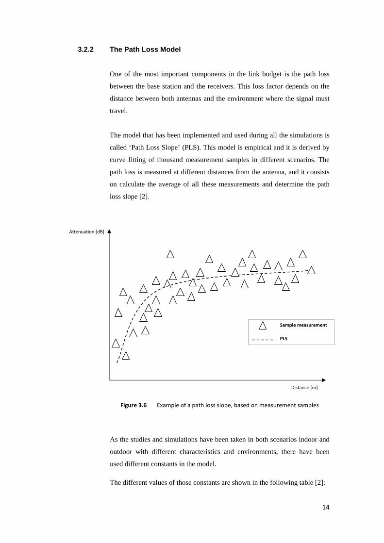
The model that has been implemented and used during all the simulations is
called ‘Path Loss Slope’ (PLS). This model is empirical and it is derived by
curve fitting of thousand measurement samples in different scenarios. The
path loss is measured at different distances from the antenna, and it consists
on calculate the average of all these measurements and determine the path
loss slope [2].
Figure 3.6 Example of a path loss slope, based on measurement samples
As the studies and simulations have been taken in both scenarios indoor and
outdoor with different characteristics and environments, there have been
used different constants in the model.
The different values of those constants are shown in the following table [2]:
Attenuation [dB]
Sample measurement
PLS
Distance [m]
15
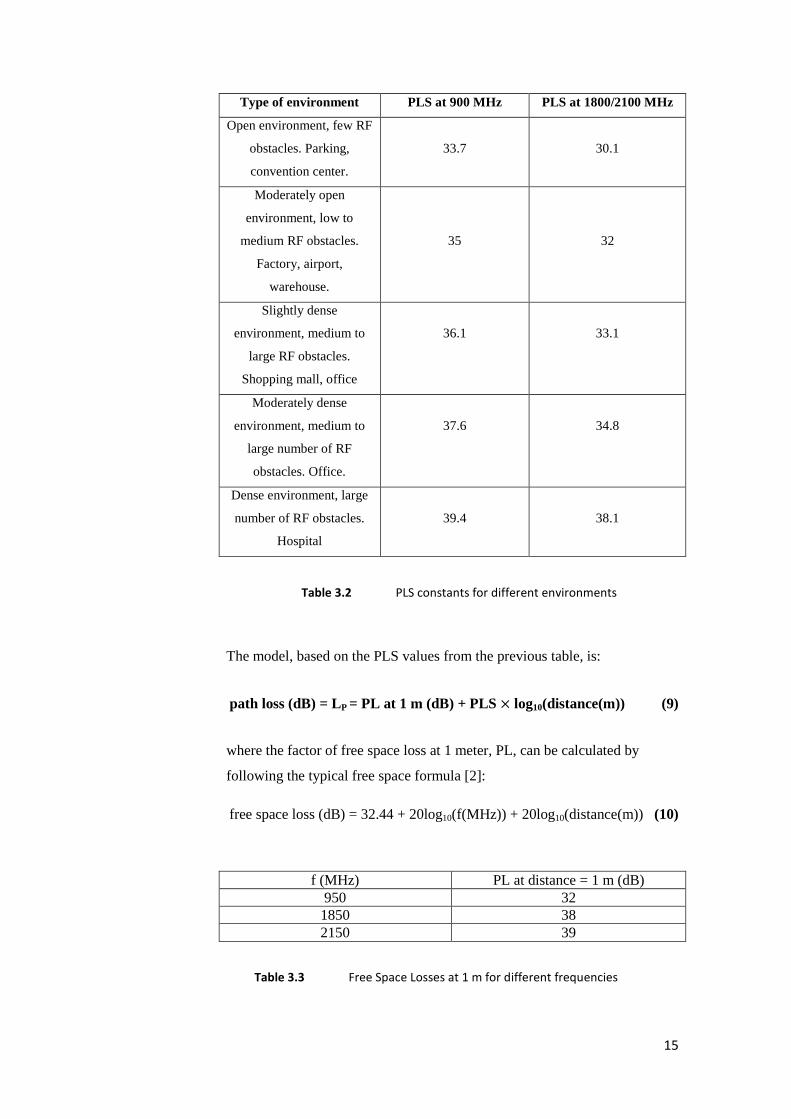
Type of environment PLS at 900 MHz PLS at 1800/2100 MHz
Open environment, few RF
obstacles. Parking,
convention center.
33.7
30.1
Moderately open
environment, low to
medium RF obstacles.
Factory, airport,
warehouse.
35
32
Slightly dense
environment, medium to
large RF obstacles.
Shopping mall, office
36.1
33.1
Moderately dense
environment, medium to
large number of RF
obstacles. Office.
37.6
34.8
Dense environment, large
number of RF obstacles.
Hospital
39.4
38.1
Table 3.2 PLS constants for different environments
The model, based on the PLS values from the previous table, is:
path loss (dB) = LP = PL at 1 m (dB) + PLS × log10(distance(m)) (9)
where the factor of free space loss at 1 meter, PL, can be calculated by
following the typical free space formula [2]:
free space loss (dB) = 32.44 + 20log10(f(MHz)) + 20log10(distance(m)) (10)
f (MHz) PL at distance = 1 m (dB) 950 32 1850 38 2150 39
Table 3.3 Free Space Losses at 1 m for different frequencies
16
3.3 Signal to Noise Ratio Since all the possible parameters that can play a role in the communication channel
between the transmitter and the receiver have been already defined in the Link Budget
section, the SNR formula can be expressed using these parameters as:
� = ��∙����∙�����∙�∙�∙��∙��∙��∙��∙��
(11)
For the particular case of the project carried out, these parameters are:
• PBS: actually in the simulations this parameter is the power measured at
the output of the connector of the remote unit (RU), PRU .
• GDAS: depending on antenna type.
• GMOB: in the simulations is supposed that the mobile antenna has no
gain.
• k: Boltzmann constant, = 1,38 × 10&'()*&+. • T: temperature, - = 290*.
• B: total available bandwidth per users. For the UMTS case, it is equal to
5 MHz per carrier.
• NF: noise figure of the mobile. Depends on the features of each mobile,
for all cases it is supposed that NF = 5 dB.
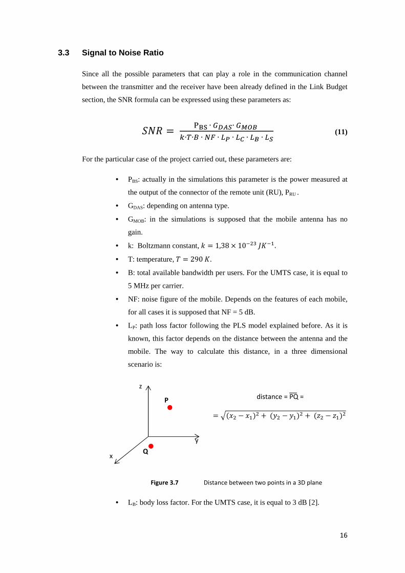
• LP: path loss factor following the PLS model explained before. As it is
known, this factor depends on the distance between the antenna and the
mobile. The way to calculate this distance, in a three dimensional
scenario is:
Figure 3.7 Distance between two points in a 3D plane
• LB: body loss factor. For the UMTS case, it is equal to 3 dB [2].
Q
P
z
y
x
distance = PQ =
= 0(2' − 2+)' +(6' − 6+)' +(7' − 7+)'
17
• LS: splitter loss factor due to the power distribution.
3.3.1 Interference Behavior
There are two different cases of interferences: additive constructively, when
all the signals from different antennas received in the User Equipment are
added; and destructive interferences, when the level of the signal in the
receiver is reduced due to the reception of other signals that come from other
antennas.
Since in this work it is modeled a one base station architecture, the signals
from the different antennas received at the User Equipment are additive.
3.4 Channel Capacity The channel capacity measures the “usable” data rate by the users. This rate will depend
on the available SNR ante available modulation and coding schemes in the system.
The expression for the capacity of the channel, C, is based on the Shannon–Hartley
theorem which states that [9], “the ideal channel capacity , meaning the theoretical
tightest upper bound on the information rate (excluding error correcting codes) of clean
(or arbitrarily low bit error rate) data that can be sent with a given average signal
power S through an analog communication channel subject to additive white Gaussian
noise of power N, is: [10]”
8 = 9 :;<' =1 + >�? = 9 :;<'(1 + �)(12)
where C is measured in bits per second, bps; B (bandwidth of the channel) in hertz, Hz,
and the SNR in linear units.
3.5 Energy Efficiency Factor The energy efficiency factor will depend on the total power required to achieve the
minimum quality value, particularly in our case, the required capacity of the channel. It
represents the required power to provide a certain capacity and it is expressed in the
following way:
@@ = A�BCB�D�EFGHDBFG�
(J/bit)(13)
18
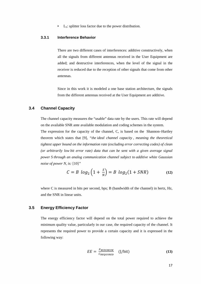
3.6 Overview of UMTS The UMTS (Universal Mobile Telecommunications System) technology offers several
advantages over its antecedent technology, GSM [3]. Meanwhile GSM is based on
using TDMA (Time Division Multiple Access) and FDMA (Frequency Division
Multiple Access) to separate users in time frequency domain, offering eight physical
channels or slots per carrier (8 users / carrier), the UMTS uses WCDMA (Wideband
Code Division Multiple Access) which is based on separating users in code domain.
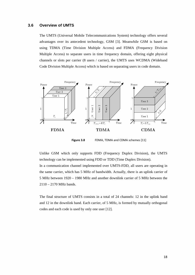
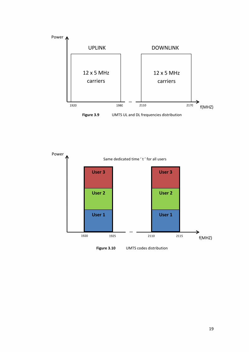
Unlike GSM which only supports FDD (Frequency Duplex Division), the UMTS
technology can be implemented using FDD or TDD (Time Duplex Division).
In a communication channel implemented over UMTS-FDD, all users are operating in
the same carrier, which has 5 MHz of bandwidth. Actually, there is an uplink carrier of
5 MHz between 1920 – 1980 MHz and another downlink carrier of 5 MHz between the
2110 – 2170 MHz bands.
The final structure of UMTS consists in a total of 24 channels: 12 in the uplink band
and 12 in the downlink band. Each carrier, of 5 MHz, is formed by mutually orthogonal
codes and each code is used by only one user [12].
Figure 3.8 FDMA, TDMA and CDMA schemes [11]
19
Figure 3.9 UMTS UL and DL frequencies distribution
Figure 3.10 UMTS codes distribution
Same dedicated time ‘ t ’ for all users
Power
f(MHZ) 1920 1925 2110 2115
1920 1980 2110 2170
Power
f(MHZ)
UPLINK DOWNLINK
12 x 5 MHz
carriers
12 x 5 MHz
carriers
User 3
User 2
User 1
User 3
User 2
User 1
User 3
User 2
User 1
…
…
Chapter 4 4.1 Outdoor Case
For the outdoor case
scenario modeling has been done looking the struct
of ‘Friends Arena Stadium’ in
This stadium has capacity for 50.000 spectators
are 105 x 68 m [13].
length of a metal structure w
to offer service to the users in the stadium. For the different simulations, it is necessary
to take the following considerations:
• The RU is connected by coax to a fixed feeder which is connecte
of the first antenna. The distance between the RU and the feeder is 10 m.
• For the path loss modeling, the scenario has been considered as an open
environment with few RF obstacles therefore the PLS constant is 30.1. Since
the operating
m factor is equal to 39
results:
• The spectators can be sitting in a space of 30 meters behind the 4 sides of the
football field as is shown in the pictures below.
Figure 4.1
30 m
30 m
Scenario Modeling
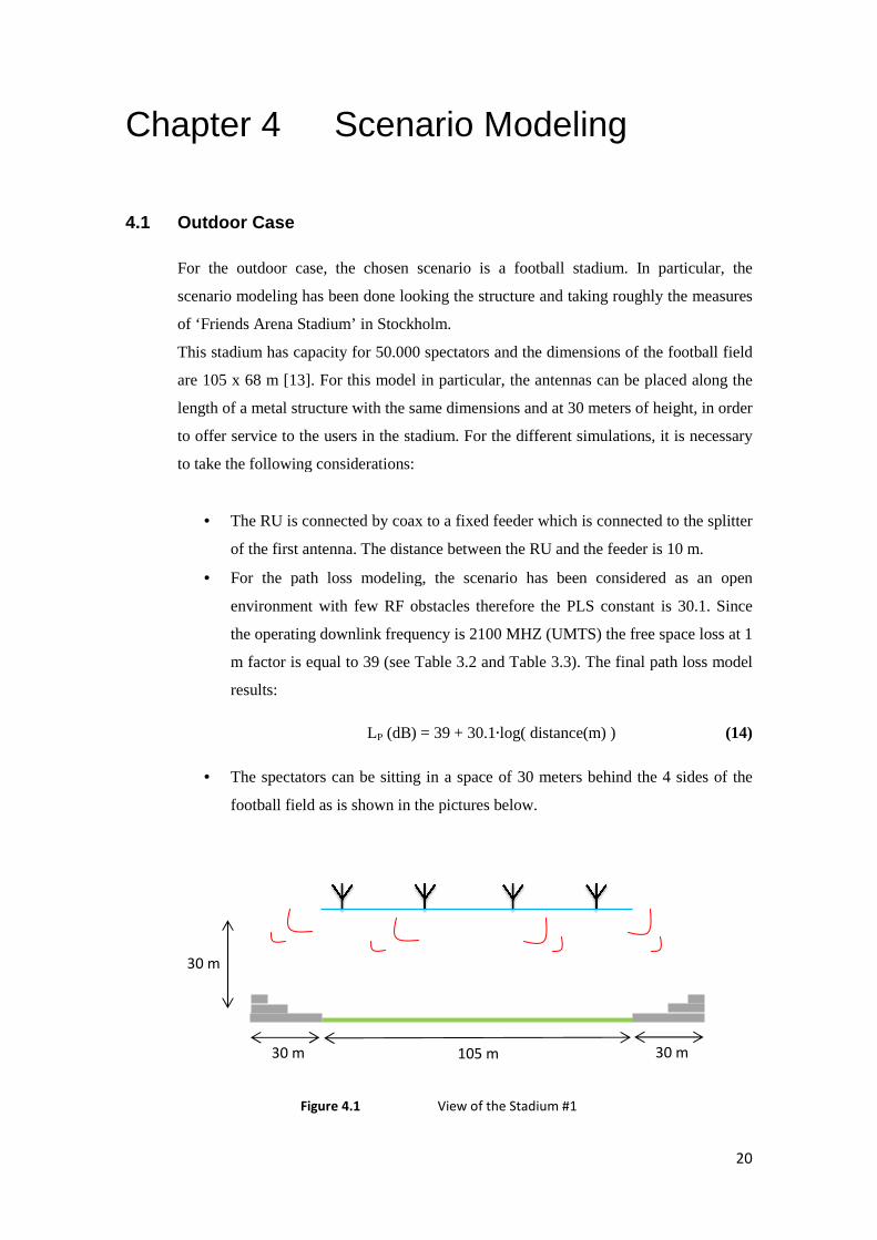
For the outdoor case, the chosen scenario is a football stadium. In particular, the
scenario modeling has been done looking the structure and taking roughly the
of ‘Friends Arena Stadium’ in Stockholm.
This stadium has capacity for 50.000 spectators and the dimensions of the football field
. For this model in particular, the antennas can be placed along
of a metal structure with the same dimensions and at 30 meters of height, in order
to offer service to the users in the stadium. For the different simulations, it is necessary
to take the following considerations:
The RU is connected by coax to a fixed feeder which is connecte
of the first antenna. The distance between the RU and the feeder is 10 m.
For the path loss modeling, the scenario has been considered as an open
environment with few RF obstacles therefore the PLS constant is 30.1. Since
downlink frequency is 2100 MHZ (UMTS) the free space loss at 1
m factor is equal to 39 (see Table 3.2 and Table 3.3). The final path loss model
LP (dB) = 39 + 30.1∙log( distance(m) )
The spectators can be sitting in a space of 30 meters behind the 4 sides of the
football field as is shown in the pictures below.
Figure 4.1 View of the Stadium #1
105 m
20
the chosen scenario is a football stadium. In particular, the
ure and taking roughly the measures
and the dimensions of the football field
For this model in particular, the antennas can be placed along the
ith the same dimensions and at 30 meters of height, in order
to offer service to the users in the stadium. For the different simulations, it is necessary
The RU is connected by coax to a fixed feeder which is connected to the splitter
of the first antenna. The distance between the RU and the feeder is 10 m.
For the path loss modeling, the scenario has been considered as an open
environment with few RF obstacles therefore the PLS constant is 30.1. Since
frequency is 2100 MHZ (UMTS) the free space loss at 1
. The final path loss model
(14)
The spectators can be sitting in a space of 30 meters behind the 4 sides of the
30 m
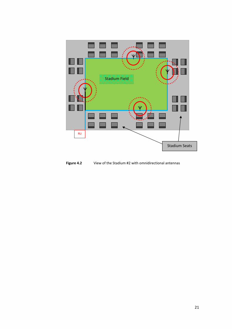
Figure 4.2
RU
View of the Stadium #2 with omnidirectional antennas
Stadium Field
Stadium Seats
21
2 with omnidirectional antennas
Stadium Seats
22
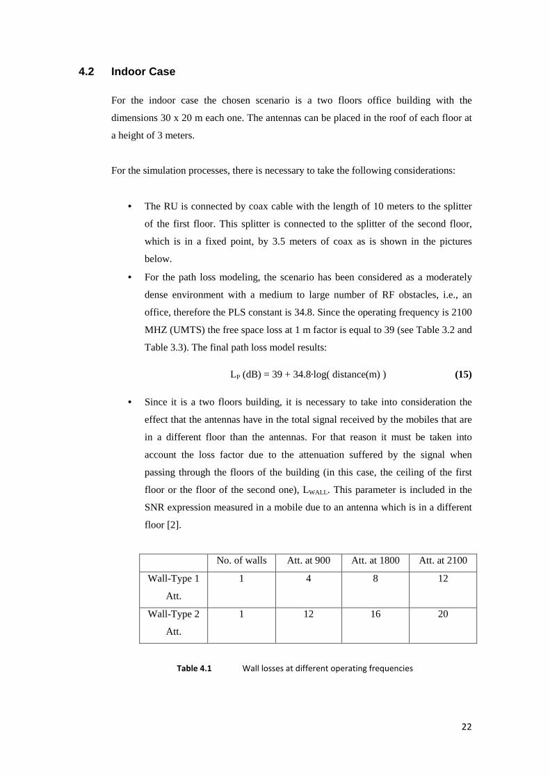
4.2 Indoor Case For the indoor case the chosen scenario is a two floors office building with the
dimensions 30 x 20 m each one. The antennas can be placed in the roof of each floor at
a height of 3 meters.
For the simulation processes, there is necessary to take the following considerations:
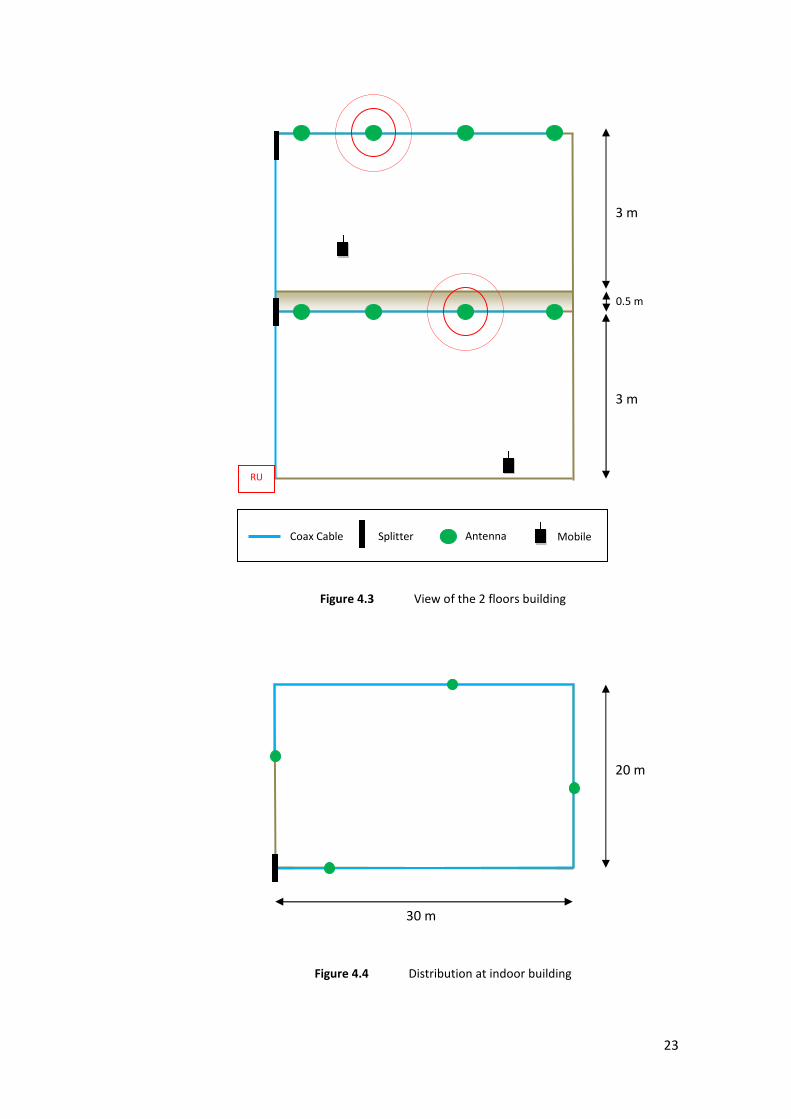
• The RU is connected by coax cable with the length of 10 meters to the splitter
of the first floor. This splitter is connected to the splitter of the second floor,
which is in a fixed point, by 3.5 meters of coax as is shown in the pictures
below.
• For the path loss modeling, the scenario has been considered as a moderately
dense environment with a medium to large number of RF obstacles, i.e., an
office, therefore the PLS constant is 34.8. Since the operating frequency is 2100
MHZ (UMTS) the free space loss at 1 m factor is equal to 39 (see Table 3.2 and
Table 3.3). The final path loss model results:
LP (dB) = 39 + 34.8∙log( distance(m) ) (15)
• Since it is a two floors building, it is necessary to take into consideration the
effect that the antennas have in the total signal received by the mobiles that are
in a different floor than the antennas. For that reason it must be taken into
account the loss factor due to the attenuation suffered by the signal when
passing through the floors of the building (in this case, the ceiling of the first
floor or the floor of the second one), LWALL . This parameter is included in the
SNR expression measured in a mobile due to an antenna which is in a different
floor [2].
No. of walls Att. at 900 Att. at 1800 Att. at 2100
Wall-Type 1
Att.
1 4 8 12
Wall-Type 2
Att.
1 12 16 20
Table 4.1 Wall losses at different operating frequencies
RU
Figure 4.3 View of the 2 floors building
Figure 4.4 Distribution at indoor building
30 m
Coax Cable Splitter MobileAntenna
23
0.5 m
Distribution at indoor building
20 m
3 m
3 m
Mobile
24
Chapter 5 Simulations 5.1 About MATLAB ®
The software used to create the different scenarios, analyze the data, develop
algorithms, run the simulations and obtain the results has been MATLAB®.
This is a high-level language and interactive environment for numerical computation,
visualization and programming [14].
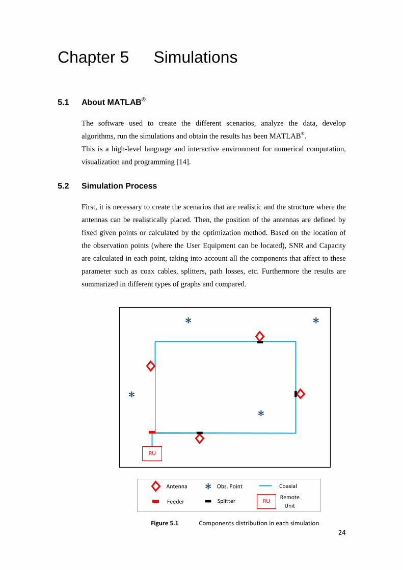
5.2 Simulation Process
First, it is necessary to create the scenarios that are realistic and the structure where the
antennas can be realistically placed. Then, the position of the antennas are defined by
fixed given points or calculated by the optimization method. Based on the location of
the observation points (where the User Equipment can be located), SNR and Capacity
are calculated in each point, taking into account all the components that affect to these
parameter such as coax cables, splitters, path losses, etc. Furthermore the results are
summarized in different types of graphs and compared.
Figure 5.1 Components distribution in each simulation
*
RU
* Antenna Obs. Point Coaxial
Feeder Splitter Remote
Unit RU
*
*
*
25
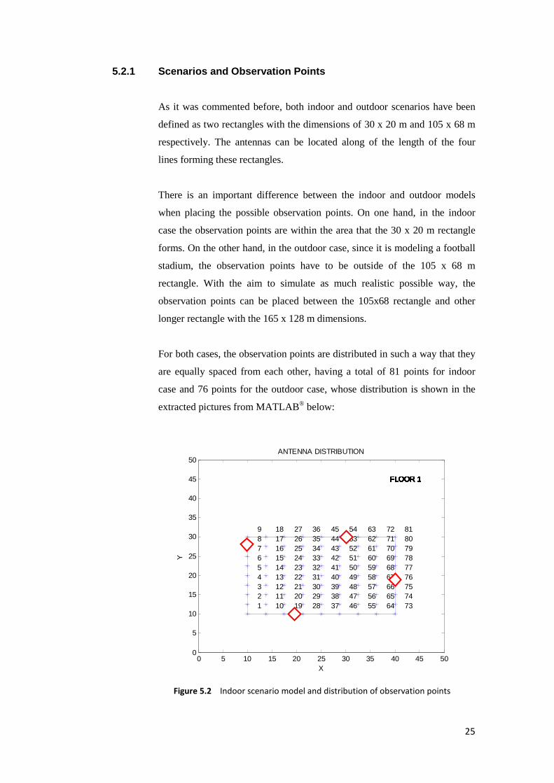
5.2.1 Scenarios and Observation Points
As it was commented before, both indoor and outdoor scenarios have been
defined as two rectangles with the dimensions of 30 x 20 m and 105 x 68 m
respectively. The antennas can be located along of the length of the four
lines forming these rectangles.
There is an important difference between the indoor and outdoor models
when placing the possible observation points. On one hand, in the indoor
case the observation points are within the area that the 30 x 20 m rectangle
forms. On the other hand, in the outdoor case, since it is modeling a football
stadium, the observation points have to be outside of the 105 x 68 m
rectangle. With the aim to simulate as much realistic possible way, the
observation points can be placed between the 105x68 rectangle and other
longer rectangle with the 165 x 128 m dimensions.
For both cases, the observation points are distributed in such a way that they
are equally spaced from each other, having a total of 81 points for indoor
case and 76 points for the outdoor case, whose distribution is shown in the
extracted pictures from MATLAB® below:
0 5 10 15 20 25 30 35 40 45 50
0
5
10
15
20
25
30
35
40
45
50ANTENNA DISTRIBUTION
X
Y
1
FLOOR 1
2
FLOOR 1
3
FLOOR 1
4
FLOOR 1
5
FLOOR 1
6
FLOOR 1
7
FLOOR 1
8
FLOOR 1
9
FLOOR 1
10
FLOOR 1
11
FLOOR 1
12
FLOOR 1
13
FLOOR 1
14
FLOOR 1
15
FLOOR 1
16
FLOOR 1
17
FLOOR 1
18
FLOOR 1
19
FLOOR 1
20
FLOOR 1
21
FLOOR 1
22
FLOOR 1
23
FLOOR 1
24
FLOOR 1
25
FLOOR 1
26
FLOOR 1
27
FLOOR 1
28
FLOOR 1
29
FLOOR 1
30
FLOOR 1
31
FLOOR 1
32
FLOOR 1
33
FLOOR 1
34
FLOOR 1
35
FLOOR 1
36
FLOOR 1
37
FLOOR 1
38
FLOOR 1
39
FLOOR 1
40
FLOOR 1
41
FLOOR 1
42
FLOOR 1
43
FLOOR 1
44
FLOOR 1
45
FLOOR 1
46
FLOOR 1
47
FLOOR 1
48
FLOOR 1
49
FLOOR 1
50
FLOOR 1
51
FLOOR 1
52
FLOOR 1
53
FLOOR 1
54
FLOOR 1
55
FLOOR 1
56
FLOOR 1
57
FLOOR 1
58
FLOOR 1
59
FLOOR 1
60
FLOOR 1
61
FLOOR 1
62
FLOOR 1
63
FLOOR 1
64
FLOOR 1
65
FLOOR 1
66
FLOOR 1
67
FLOOR 1
68
FLOOR 1
69
FLOOR 1
70
FLOOR 1
71
FLOOR 1
72
FLOOR 1
73
FLOOR 1
74
FLOOR 1
75
FLOOR 1
76
FLOOR 1
77
FLOOR 1
78
FLOOR 1
79
FLOOR 1
80
FLOOR 1
81
FLOOR 1
Figure 5.2 Indoor scenario model and distribution of observation points
26
0 20 40 60 80 100 120 140 1600
20
40
60
80
100
120
STADIUM
X
Y
1
2
3
4
5
6
7
8
9
10
11
12
13
14
15
16
17
18
19
20
21
22
23
24
25
26
27
28
29
30
31
32
33
34
35
36
37
38
39
40
41
42
43
44
45
46
47
48
49
50
51
52
53
54
55
56
57
58
59
60
61
62
63
64
65
66
67
68
69
70
71
72
73
74
75
76
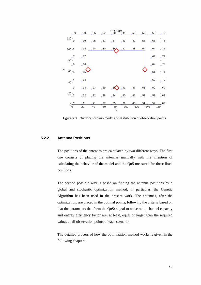
5.2.2 Antenna Positions
The positions of the antennas are calculated by two different ways. The first
one consists of placing the antennas manually with the intention of
calculating the behavior of the model and the QoS measured for these fixed
positions.
The second possible way is based on finding the antenna positions by a
global and stochastic optimization method. In particular, the Genetic
Algorithm has been used in the present work. The antennas, after the
optimization, are placed in the optimal points, following the criteria based on
that the parameters that form the QoS: signal to noise ratio, channel capacity
and energy efficiency factor are, at least, equal or larger than the required
values at all observation points of each scenario.
The detailed process of how the optimization method works is given in the
following chapters.
Figure 5.3 Outdoor scenario model and distribution of observation points

27
5.2.3 Calculation of QoS Parameters
Once the antenna positions and observation points are known, the final step
is to calculate the parameters that define the quality of service by applying
the formulas detailed before. All the calculations are made by different
MATLAB ® functions, whose results will be different depending on the type
of scenario selected and on the given input parameters. When calculating the
SNR values in each observation point there are a few parameters that vary
depending on the positions of the antennas and the measurement points, such
as losses factors.
The positions of the antennas and the observation points allow to:
i. Calculate the path losses, LP, depending on the distances between
each antenna and each observation point.
The antenna positions allow to:
ii. Calculate the losses due to coaxial, LC, depending on the different
distances between each antenna. It is also taken into account the 10
meters of coax between the RU and the feeder.
The number of the antennas allow to:
iii. Calculate the losses due to the splitters, LS, depending also on the
different power distribution ratio of each splitter
Once the SNR values are calculated, one can immediately find out the
corresponding capacity values and then the energy saving factor.
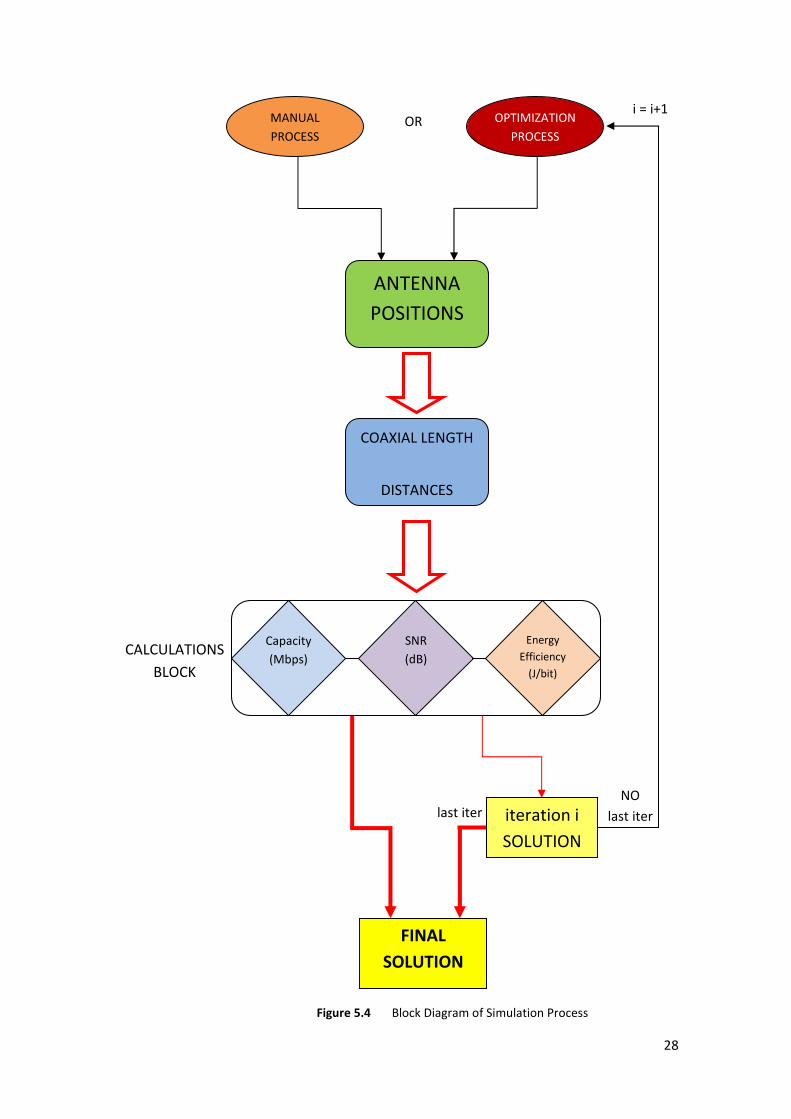
5.2.4 Phase Diagram
For a better explanation of how the simulations are done and what its phases
and functions are, it is attached the blocks diagram below:
28
Figure 5.4 Block Diagram of Simulation Process
CALCULATIONS
BLOCK
last iter
i = i+1 MANUAL
PROCESS
OPTIMIZATION
PROCESS
COAXIAL LENGTH
DISTANCES
ANTENNA
POSITIONS
SNR
(dB)
Energy
Efficiency
(J/bit)
Capacity
(Mbps)
FINAL
SOLUTION
OR
iteration i
SOLUTION
NO
last iter
29
Chapter 6 Optimization 6.1 Overview of Genetic Algorithm
The main idea of the genetic algorithm came from Charles Darwin’s theory of
evolution: natural selection or survival of the fittest [15]. A genetic algorithm is a
stochastic method that searches for the global minimum in a discrete search space. As
an optimizer, the powerful heuristic of the genetic algorithm is effective at solving
complex, combinational and related problems [16].
Genes are the basic building blocks in a genetic algorithm and each of them consists of
a binary encoding of a parameter. The number of genes per parameter is determined by
the accuracy with which the parameter should be reconstructed. When all the
parameters that should be determined have been translated into the genes, they comprise
a chromosome [16]. Each chromosome is associated with a value of objective
functional, in other words, a value of a previously defined cost function.
The genetic algorithm starts from an initial population which is generated randomly.
Then, the values of the cost function are evaluated for each chromosome in the
population, and the chromosomes are sorted in the order of the cost function values
(ranking), depending on if the goal is to maximize or minimize that cost function. The
part of the chromosomes which have the worst objective functional values is discarded
and the rest of the chromosomes are used for mating, which is a process where the
chromosomes exchange genes to produce new chromosomes called offspring [16].
Correspondingly, the chromosomes which are used for the mating are referred to as
parents. To produce the offspring, two chromosomes are chosen from the parents by a
selection procedure, for example, proportional (roulette-wheel) or tournament selection
[15]. The selected chromosomes are then used to produce two offspring by the
crossover operator, for example, one-point, N-point or uniform crossover operators.
30
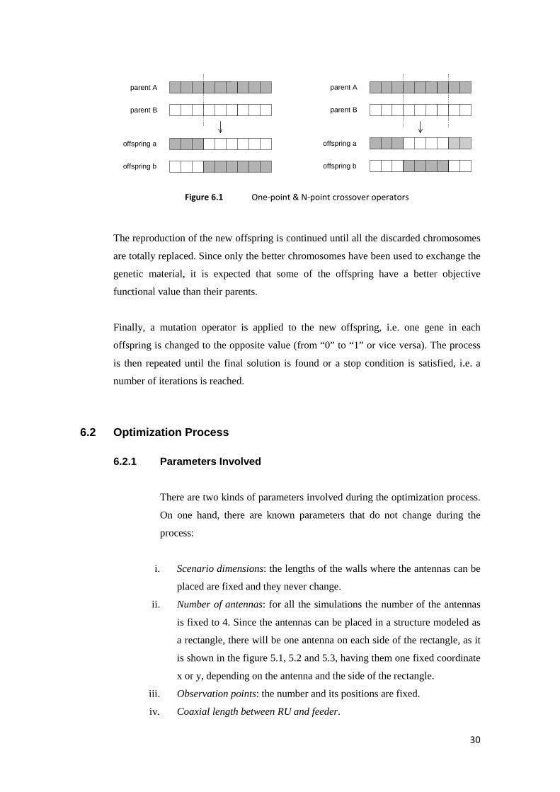
Figure 6.1 One-point & N-point crossover operators
The reproduction of the new offspring is continued until all the discarded chromosomes
are totally replaced. Since only the better chromosomes have been used to exchange the
genetic material, it is expected that some of the offspring have a better objective
functional value than their parents.
Finally, a mutation operator is applied to the new offspring, i.e. one gene in each
offspring is changed to the opposite value (from “0” to “1” or vice versa). The process
is then repeated until the final solution is found or a stop condition is satisfied, i.e. a
number of iterations is reached.
6.2 Optimization Process
6.2.1 Parameters Involved
There are two kinds of parameters involved during the optimization process.
On one hand, there are known parameters that do not change during the
process:
i. Scenario dimensions: the lengths of the walls where the antennas can be
placed are fixed and they never change.
ii. Number of antennas: for all the simulations the number of the antennas
is fixed to 4. Since the antennas can be placed in a structure modeled as
a rectangle, there will be one antenna on each side of the rectangle, as it
is shown in the figure 5.1, 5.2 and 5.3, having them one fixed coordinate
x or y, depending on the antenna and the side of the rectangle.
iii. Observation points: the number and its positions are fixed.
iv. Coaxial length between RU and feeder.
parent A
parent B
offspring a
offspring b
parent A
parent B
offspring a
offspring b
31
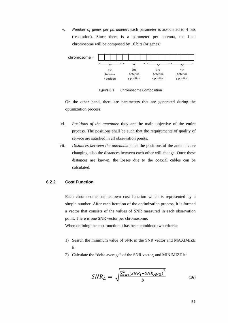
v. Number of genes per parameter: each parameter is associated to 4 bits
(resolution). Since there is a parameter per antenna, the final
chromosome will be composed by 16 bits (or genes):
Figure 6.2 Chromosome Composition
On the other hand, there are parameters that are generated during the
optimization process:
vi. Positions of the antennas: they are the main objective of the entire
process. The positions shall be such that the requirements of quality of
service are satisfied in all observation points.
vii. Distances between the antennas: since the positions of the antennas are
changing, also the distances between each other will change. Once these
distances are known, the losses due to the coaxial cables can be
calculated.
6.2.2 Cost Function
Each chromosome has its own cost function which is represented by a
simple number. After each iteration of the optimization process, it is formed
a vector that consists of the values of SNR measured in each observation
point. There is one SNR vector per chromosome.
When defining the cost function it has been combined two criteria:
1) Search the minimum value of SNR in the SNR vector and MAXIMIZE
it.
2) Calculate the “delta average” of the SNR vector, and MINIMIZE it:
�∆ =O∑ (>�QR&>�Q�ST)URVWX
Y (16)
chromosome =
1st
Antenna
x position
2nd
Antenna
y position
3rd
Antenna
x position
4th
Antenna
y position
32
where:
�∆ = Z[:\]_]_[`]<[;a�
�bc� = �]_[`]<[ d = efgd[`;a;dh[`_]\i;ehj;ie\h
The second criterion is introduced with the aim to do not have notable
differences between the maximum and minimum SNR values, providing a
more uniform coverage. However, since the principal objective is to
maximize the minimum SNR value it is added a scaling coefficient α, whose
values vary between 0 and 1, in order to emphasize the first criterion over
the second one.
In this manner, the cost function is constructed as follows:
8k = �lm� − n ∙ �∆ (17)
With this definition, the goal is to find such positions of the antennas that
maximize the cost function.
6.2.3 Applying Genetic Algorithm
As it was described earlier, the first step consists of generating what is called
random population. For all cases in the simulations, this population is
composed by a total of 100 chromosomes of 16 bits each one. With this
population it is calculated the corresponding antennas positions and the
measured SNR in the observation points.
The second step is to compute the cost function associated to the population.
It is calculated the cost function values of each chromosome following the
two criteria explained before. Then, the chromosomes are sorted, being the
chromosome with the highest cost function value at the top of this rank.
The next step consists of selecting the parents by rejecting the second half of
the population, which has the worst cost function values. Once the parents
are selected, the offspring is formed by choosing pairs of chromosomes
randomly using the one-point crossover method (see Figure 6.1).
33
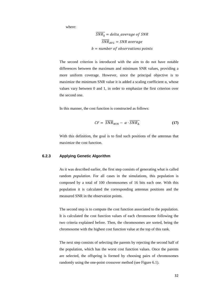
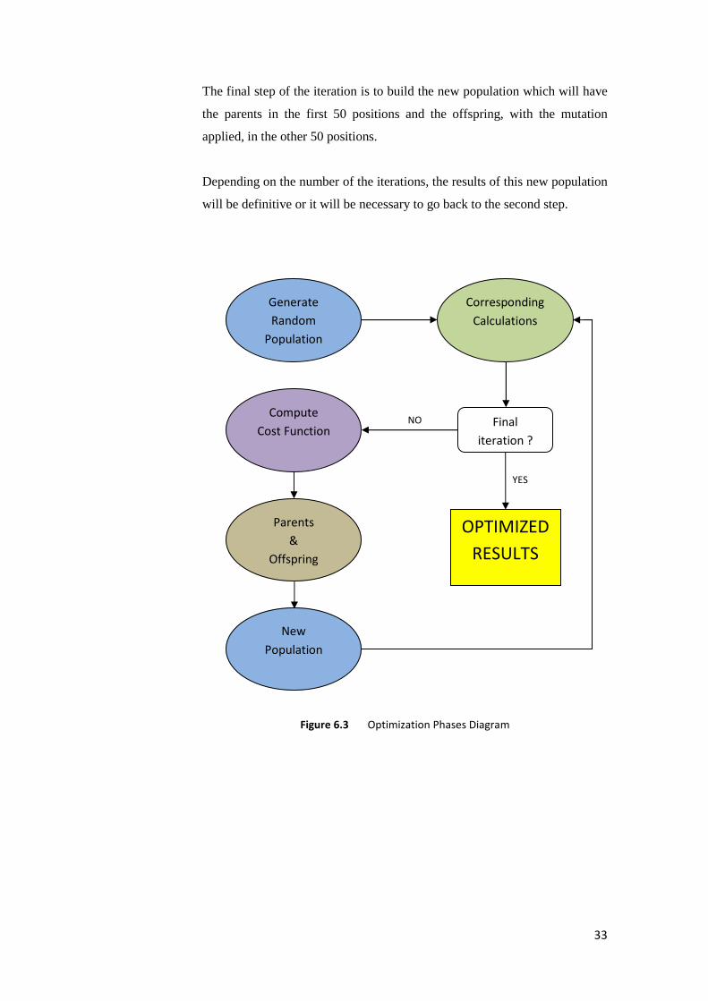
The final step of the iteration is to build the new population which will have
the parents in the first 50 positions and the offspring, with the mutation
applied, in the other 50 positions.
Depending on the number of the iterations, the results of this new population
will be definitive or it will be necessary to go back to the second step.
Figure 6.3 Optimization Phases Diagram
YES
NO
Generate
Random
Population
Compute
Cost Function
Parents
&
Offspring
New
Population
Corresponding
Calculations
OPTIMIZED
RESULTS
Final
iteration ?
34
Chapter 7 Showcases & Results 7.1 Required Quality of Service
The selected criterion, since it is being studied a 3G connection, has been that the
measured level of capacity in the worst case (single point to point link) has to be no less
than 10 Mbps. In most of cases, unless otherwise indicated, there is one base station,
one MU and only one RU which is emitting the same frequency channel through the
antenna system. Since the available bandwidth for this case (UMTS) is 5 MHz, applying
the Shannon Theorem as it is shown in the formula 10, the minimum SNR level must be
4.77 dB in the worst case. This criterion is applied in all the cases that have been
simulated and optimized.
7.2 Showcases Description Below, is explained in detail what is calculated in each simulated case and the purposes
of why the simulations have been carried out during the project. Also it is given the
description of the scenarios and the different considerations that are taken in each case.
7.2.1 Efficiency Trends Case
The objective of this case is to compare the minimum power values required
to achieve the defined quality of service. It is studied in both scenarios,
outdoor and indoor.
The simulation consists of investigating the minimum power levels required
for the different cases of one, two and four antennas distributed along the
scenario. Furthermore, the effects of the coax cable losses, the splitting ratios
of the splitters and the directivity of the antennas, are presented.
7.2.2 Optimization Case
With the elaboration of this case, the intention is to investigate the effect of
the position of the antennas on the energy saving. The optimal positions of
the antennas, by using the global optimization method, are obtained by
following the criteria explained before. For all cases, the term ‘α’ of the
35
second criterion is equal to 0 with the aim of using the cost function to
maximize the minimum SNR value. Then, it is calculated the minimum
power to achieve the required conditions of quality and it is compared to the
obtained values when the positions of the antennas are fixed manually, i.e. in
the corners, in the middle of each wall, etc.
This model is implemented for both indoor and outdoor cases, taking into
account and not taking into account the losses due to the coaxial and using
different types of splitters. By using the outdoor case the aim is to analyze
the different power consumptions in relation with the position of the
antennas. Moreover, by using the indoor case the goal is to investigate the
effect that the interferences have in a two floors building and how they could
affect when calculating the antenna positions with the optimization process.
7.2.3 Optical – Wireless Case
Since the entire architecture of this DAS in the outdoor case is composed by
an optical and a wireless part, in this case both parts have been taken into
consideration when calculating the total power consumption.
For the optical part, it is taken into account the power required by an optical
fiber to feed the remote unit that belongs to the wireless part. In this case,
unlike the rest, there is one remote unit per antenna and they are connected
by a very short coax cable whose losses can be neglected. The cases of one,
two, four, six and eight antennas are analyzed.
7.3 Simulations In each simulation it is shown the scenario with the positions of the antennas and the
distribution of the total observation points. Besides, the SNR values are shown in a level
graph representing the value in each observation point and the capacity values are
indicated in a levels curves graph, where it is easy to identify the measured level by the
attached color scale. The corresponding distribution of the observation points is
available in the previous pictures Figure 5.2 and Figure 5.3.
36
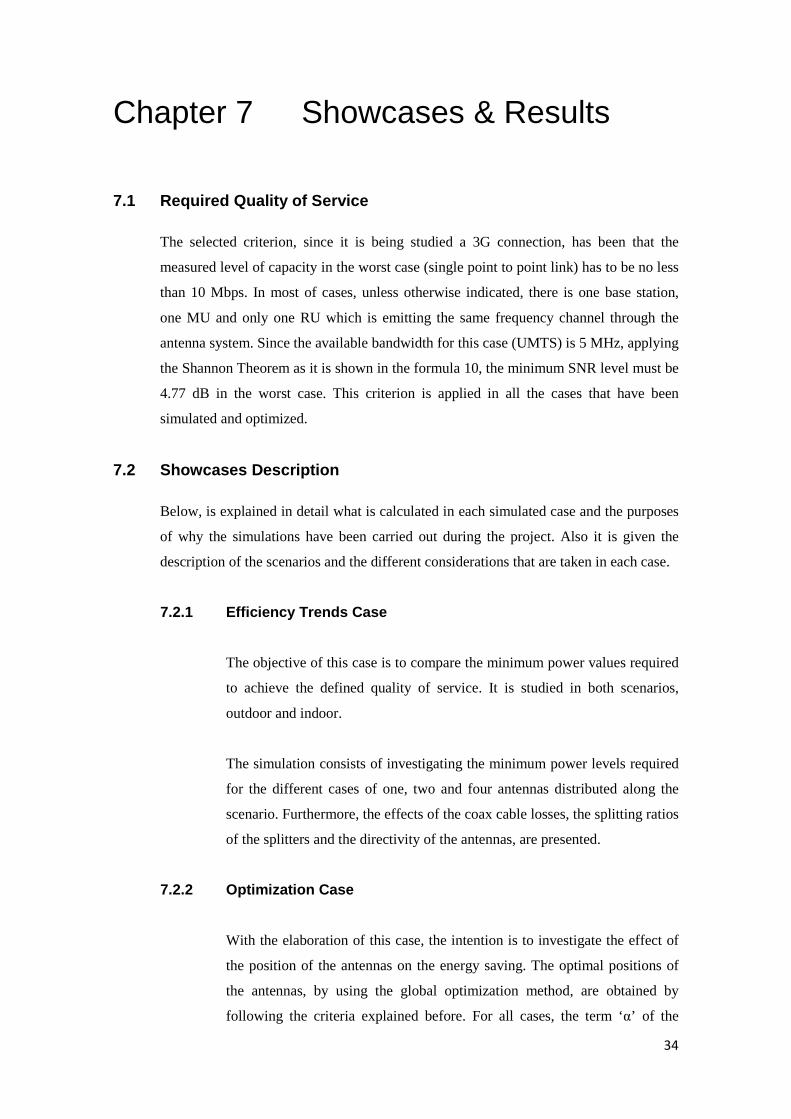
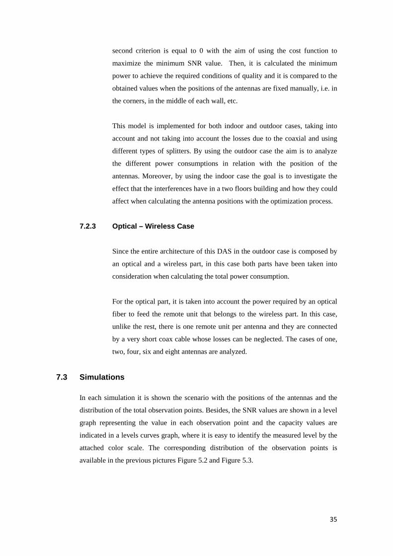
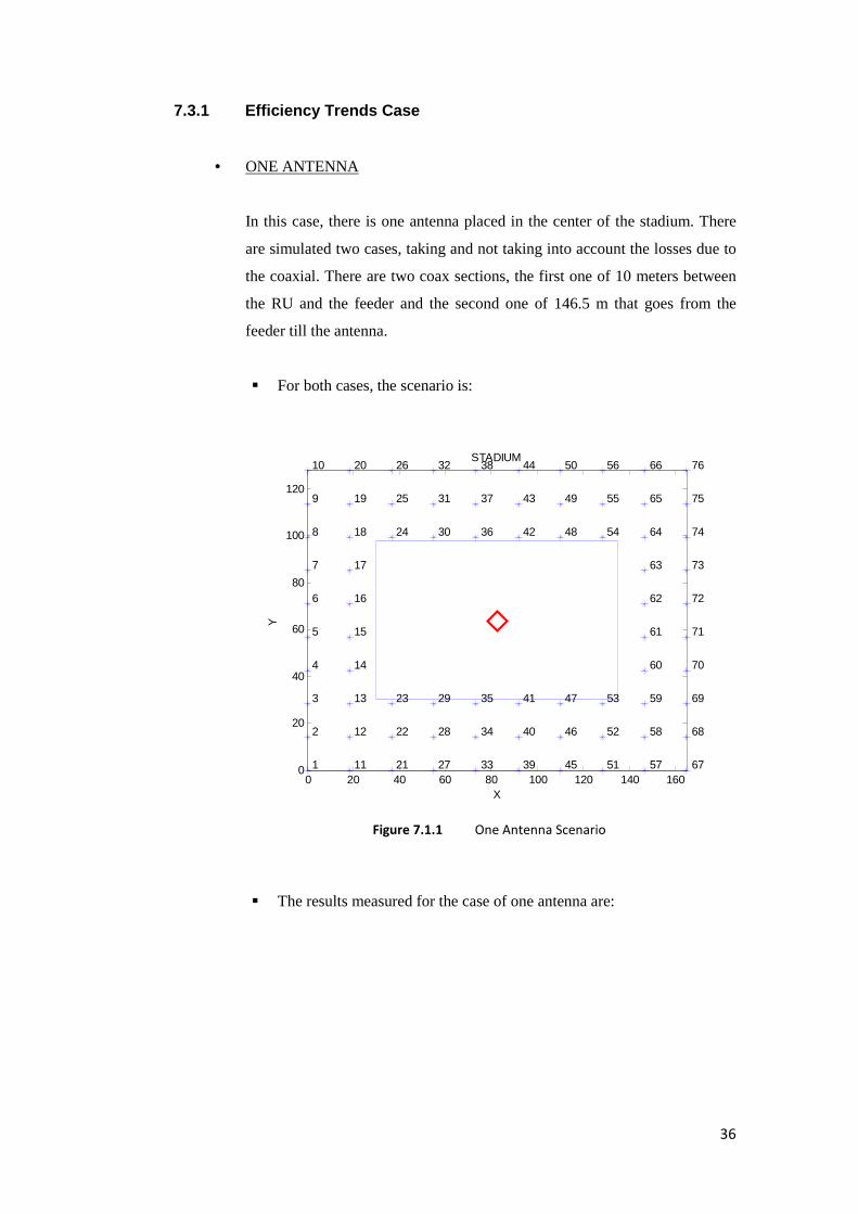
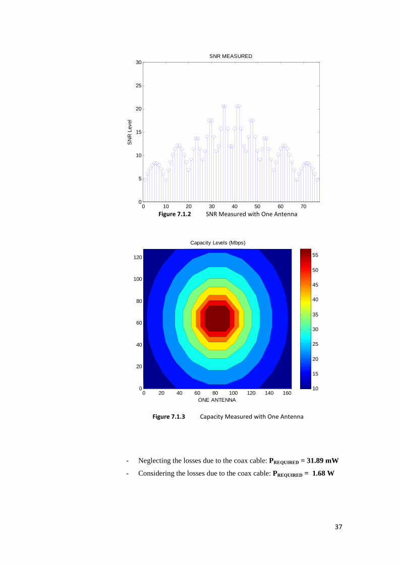
7.3.1 Efficiency Trends Case
• ONE ANTENNA
In this case, there is one antenna placed in the center of the stadium. There
are simulated two cases, taking and not taking into account the losses due to
the coaxial. There are two coax sections, the first one of 10 meters between
the RU and the feeder and the second one of 146.5 m that goes from the
feeder till the antenna.
� For both cases, the scenario is:
� The results measured for the case of one antenna are:
0 20 40 60 80 100 120 140 1600
20
40
60
80
100
120
STADIUM
X
Y
1
2
3
4
5
6
7
8
9
10
11
12
13
14
15
16
17
18
19
20
21
22
23
24
25
26
27
28
29
30
31
32
33
34
35
36
37
38
39
40
41
42
43
44
45
46
47
48
49
50
51
52
53
54
55
56
57
58
59
60
61
62
63
64
65
66
67
68
69
70
71
72
73
74
75
76
Figure 7.1.1 One Antenna Scenario
37
0 10 20 30 40 50 60 700
5
10
15
20
25
30SNR MEASURED
Observation Points
SN
R L
evel
- Neglecting the losses due to the coax cable: PREQUIRED = 31.89 mW
- Considering the losses due to the coax cable: PREQUIRED = 1.68 W
ONE ANTENNA
Capacity Levels (Mbps)
0 20 40 60 80 100 120 140 1600
20
40
60
80
100
120
10
15
20
25
30
35
40
45
50
55
Figure 7.1.2 SNR Measured with One Antenna
Figure 7.1.3 Capacity Measured with One Antenna
38
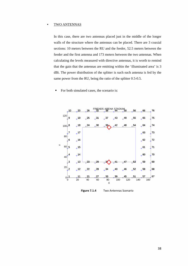
• TWO ANTENNAS
In this case, there are two antennas placed just in the middle of the longer
walls of the structure where the antennas can be placed. There are 3 coaxial
sections: 10 meters between the RU and the feeder, 52.5 meters between the
feeder and the first antenna and 173 meters between the two antennas. When
calculating the levels measured with directive antennas, it is worth to remind
that the gain that the antennas are emitting within the ‘illuminated area’ is 3
dBi. The power distribution of the splitter is such each antenna is fed by the
same power from the RU, being the ratio of the splitter 0.5-0.5.
� For both simulated cases, the scenario is:
0 20 40 60 80 100 120 140 1600
20
40
60
80
100
120
FRIENDS ARENA STADIUM
X
Y
1
2
3
4
5
6
7
8
9
10
11
12
13
14
15
16
17
18
19
20
21
22
23
24
25
26
27
28
29
30
31
32
33
34
35
36
37
38
39
40
41
42
43
44
45
46
47
48
49
50
51
52
53
54
55
56
57
58
59
60
61
62
63
64
65
66
67
68
69
70
71
72
73
74
75
76
1
2
3
4
5
6
7
8
9
10
11
12
13
14
15
16
17
18
19
20
21
22
23
24
25
26
27
28
29
30
31
32
33
34
35
36
37
38
39
40
41
42
43
44
45
46
47
48
49
50
51
52
53
54
55
56
57
58
59
60
61
62
63
64
65
66
67
68
69
70
71
72
73
74
75
76
Figure 7.1.4 Two Antennas Scenario
39
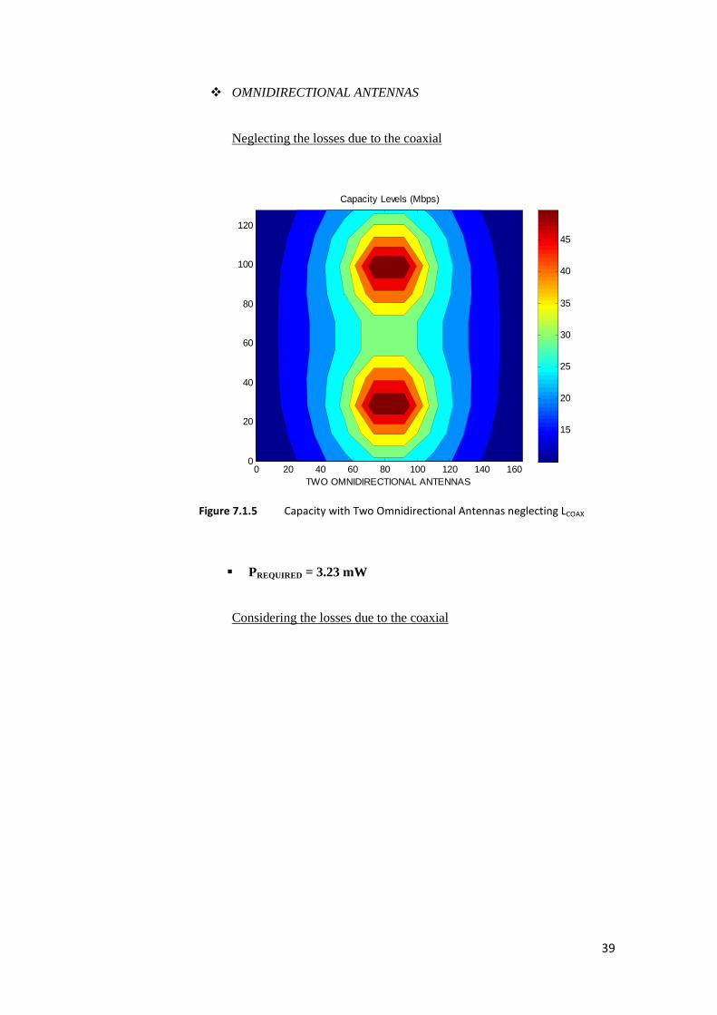
� OMNIDIRECTIONAL ANTENNAS
Neglecting the losses due to the coaxial
� PREQUIRED = 3.23 mW
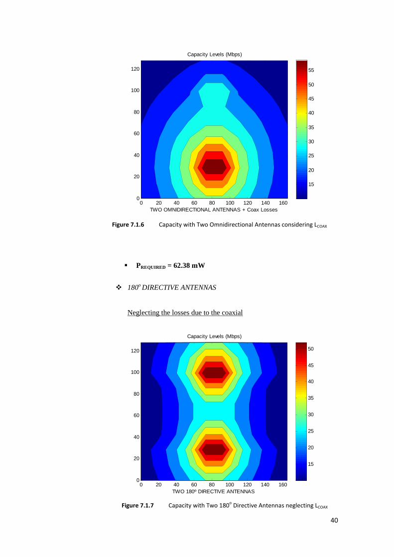
Considering the losses due to the coaxial
TWO OMNIDIRECTIONAL ANTENNAS
Capacity Levels (Mbps)
0 20 40 60 80 100 120 140 1600
20
40
60
80
100
120
15
20
25
30
35
40
45
Figure 7.1.5 Capacity with Two Omnidirectional Antennas neglecting LCOAX
40
� PREQUIRED = 62.38 mW
� 180o DIRECTIVE ANTENNAS
Neglecting the losses due to the coaxial
TWO OMNIDIRECTIONAL ANTENNAS + Coax Losses
Capacity Levels (Mbps)
0 20 40 60 80 100 120 140 1600
20
40
60
80
100
120
15
20
25
30
35
40
45
50
55
TWO 180º DIRECTIVE ANTENNAS
Capacity Levels (Mbps)
0 20 40 60 80 100 120 140 1600
20
40
60
80
100
120
15
20
25
30
35
40
45
50
Figure 7.1.6 Capacity with Two Omnidirectional Antennas considering LCOAX
Figure 7.1.7 Capacity with Two 180o Directive Antennas neglecting LCOAX
41
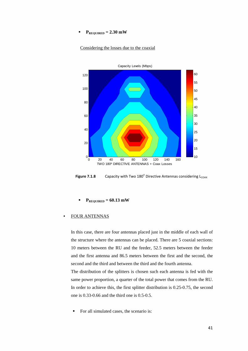
� PREQUIRED = 2.30 mW
Considering the losses due to the coaxial
� PREQUIRED = 60.13 mW
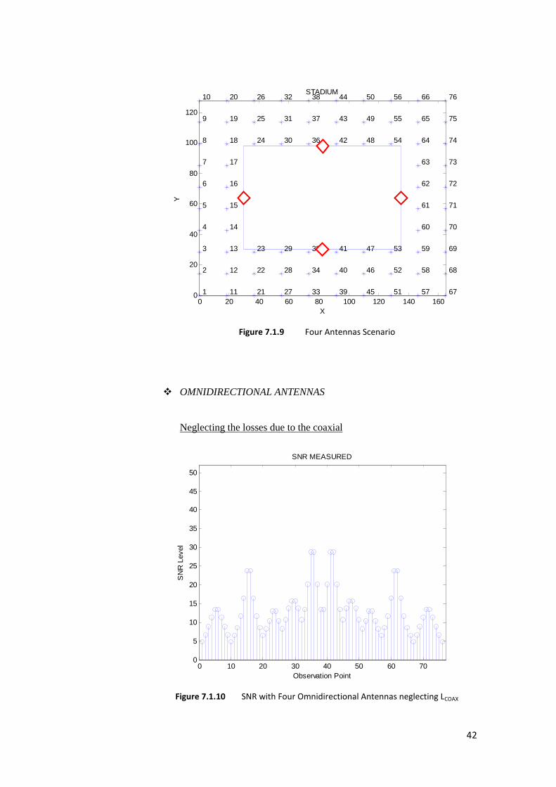
• FOUR ANTENNAS
In this case, there are four antennas placed just in the middle of each wall of
the structure where the antennas can be placed. There are 5 coaxial sections:
10 meters between the RU and the feeder, 52.5 meters between the feeder
and the first antenna and 86.5 meters between the first and the second, the
second and the third and between the third and the fourth antenna.
The distribution of the splitters is chosen such each antenna is fed with the
same power proportion, a quarter of the total power that comes from the RU.
In order to achieve this, the first splitter distribution is 0.25-0.75, the second
one is 0.33-0.66 and the third one is 0.5-0.5.
� For all simulated cases, the scenario is:
TWO 180º DIRECTIVE ANTENNAS + Coax Losses
Capacity Levels (Mbps)
0 20 40 60 80 100 120 140 1600
20
40
60
80
100
120
10
15
20
25
30
35
40
45
50
55
60
Figure 7.1.8 Capacity with Two 180o Directive Antennas considering LCOAX
42
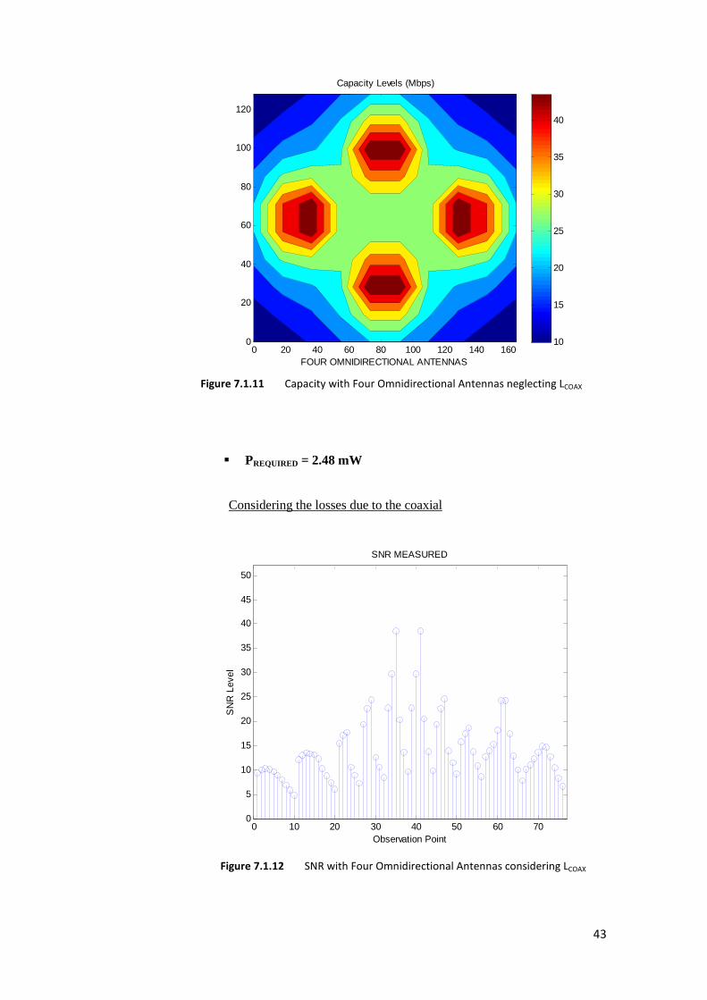
� OMNIDIRECTIONAL ANTENNAS
Neglecting the losses due to the coaxial
0 20 40 60 80 100 120 140 1600
20
40
60
80
100
120
STADIUM
X
Y
1
2
3
4
5
6
7
8
9
10
11
12
13
14
15
16
17
18
19
20
21
22
23
24
25
26
27
28
29
30
31
32
33
34
35
36
37
38
39
40
41
42
43
44
45
46
47
48
49
50
51
52
53
54
55
56
57
58
59
60
61
62
63
64
65
66
67
68
69
70
71
72
73
74
75
76
0 10 20 30 40 50 60 700
5
10
15
20
25
30
35
40
45
50
SNR MEASURED
Observation Point
SN
R L
evel
Figure 7.1.9 Four Antennas Scenario
Figure 7.1.10 SNR with Four Omnidirectional Antennas neglecting LCOAX
43
� PREQUIRED = 2.48 mW
Considering the losses due to the coaxial
FOUR OMNIDIRECTIONAL ANTENNAS
Capacity Levels (Mbps)
0 20 40 60 80 100 120 140 1600
20
40
60
80
100
120
10
15
20
25
30
35
40
0 10 20 30 40 50 60 700
5
10
15
20
25
30
35
40
45
50
SNR MEASURED
Observation Point
SN
R L
evel
Figure 7.1.11 Capacity with Four Omnidirectional Antennas neglecting LCOAX
Figure 7.1.12 SNR with Four Omnidirectional Antennas considering LCOAX
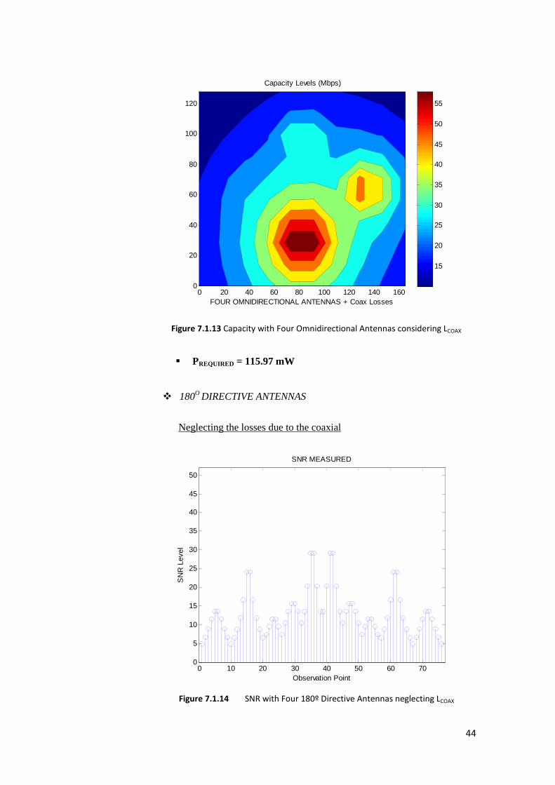
44
� PREQUIRED = 115.97 mW
� 180O DIRECTIVE ANTENNAS Neglecting the losses due to the coaxial
FOUR OMNIDIRECTIONAL ANTENNAS + Coax Losses
Capacity Levels (Mbps)
0 20 40 60 80 100 120 140 1600
20
40
60
80
100
120
15
20
25
30
35
40
45
50
55
0 10 20 30 40 50 60 700
5
10
15
20
25
30
35
40
45
50
SNR MEASURED
Observation Point
SN
R L
evel
Figure 7.1.13 Capacity with Four Omnidirectional Antennas considering LCOAX
Figure 7.1.14 SNR with Four 180º Directive Antennas neglecting LCOAX
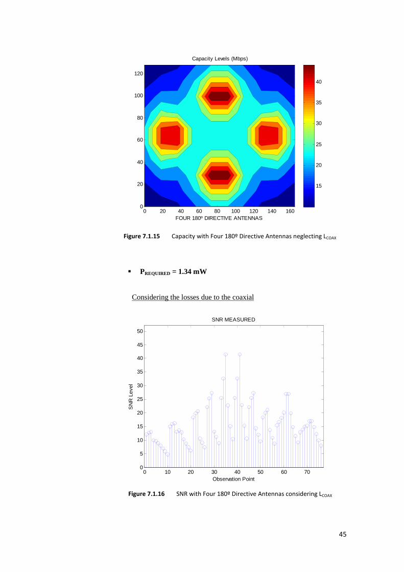
45
0 10 20 30 40 50 60 700
5
10
15
20
25
30
35
40
45
50
SNR MEASURED
Observation Point
SN
R L
evel
� PREQUIRED = 1.34 mW
Considering the losses due to the coaxial
FOUR 180º DIRECTIVE ANTENNAS
Capacity Levels (Mbps)
0 20 40 60 80 100 120 140 1600
20
40
60
80
100
120
15
20
25
30
35
40
Figure 7.1.15 Capacity with Four 180º Directive Antennas neglecting LCOAX
Figure 7.1.16 SNR with Four 180º Directive Antennas considering LCOAX
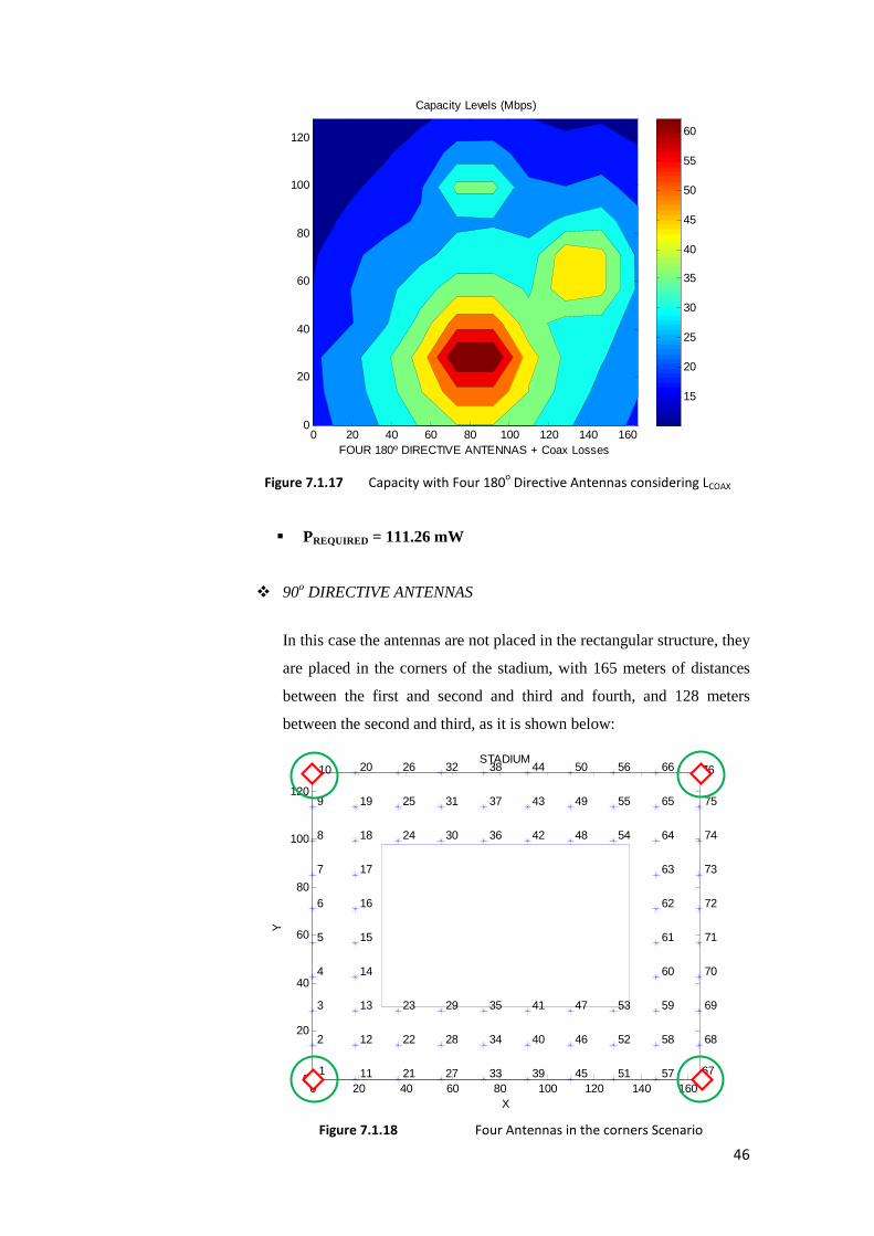
46
0 20 40 60 80 100 120 140 1600
20
40
60
80
100
120
STADIUM
X
Y
1
2
3
4
5
6
7
8
9
10
11
12
13
14
15
16
17
18
19
20
21
22
23
24
25
26
27
28
29
30
31
32
33
34
35
36
37
38
39
40
41
42
43
44
45
46
47
48
49
50
51
52
53
54
55
56
57
58
59
60
61
62
63
64
65
66
67
68
69
70
71
72
73
74
75
76
� PREQUIRED = 111.26 mW
� 90o DIRECTIVE ANTENNAS
In this case the antennas are not placed in the rectangular structure, they
are placed in the corners of the stadium, with 165 meters of distances
between the first and second and third and fourth, and 128 meters
between the second and third, as it is shown below:
FOUR 180º DIRECTIVE ANTENNAS + Coax Losses
Capacity Levels (Mbps)
0 20 40 60 80 100 120 140 1600
20
40
60
80
100
120
15
20
25
30
35
40
45
50
55
60
Figure 7.1.17 Capacity with Four 180o Directive Antennas considering LCOAX
Figure 7.1.18 Four Antennas in the corners Scenario
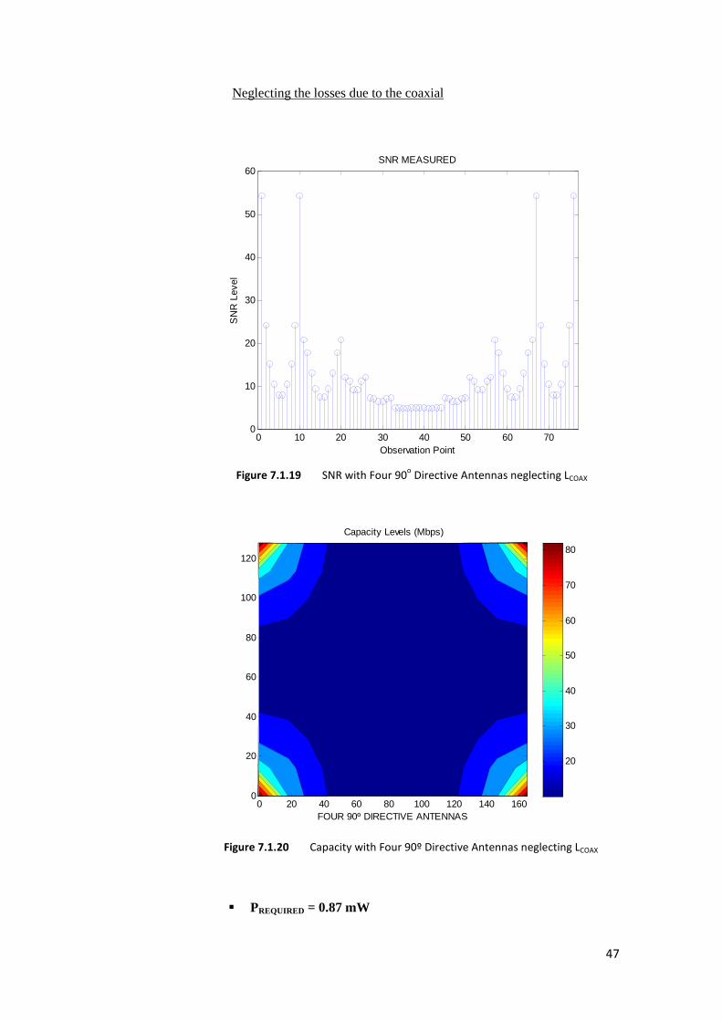
47
Neglecting the losses due to the coaxial
�
� PREQUIRED = 0.87 mW
0 10 20 30 40 50 60 700
10
20
30
40
50
60SNR MEASURED
Observation Point
SN
R L
evel
FOUR 90º DIRECTIVE ANTENNAS
Capacity Levels (Mbps)
0 20 40 60 80 100 120 140 1600
20
40
60
80
100
120
20
30
40
50
60
70
80
Figure 7.1.20 Capacity with Four 90º Directive Antennas neglecting LCOAX
Figure 7.1.19 SNR with Four 90o Directive Antennas neglecting LCOAX
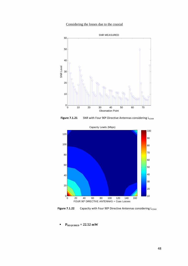
48
Considering the losses due to the coaxial
� PREQUIRED = 22.52 mW
0 10 20 30 40 50 60 700
10
20
30
40
50
60SNR MEASURED
Observation Point
SN
R L
evel
FOUR 90º DIRECTIVE ANTENNAS + Coax Losses
Capacity Levels (Mbps)
0 20 40 60 80 100 120 140 1600
20
40
60
80
100
120
10
20
30
40
50
60
70
80
90
100
Figure 7.1.21 SNR with Four 90º Directive Antennas considering LCOAX
Figure 7.1.22 Capacity with Four 90º Directive Antennas considering LCOAX
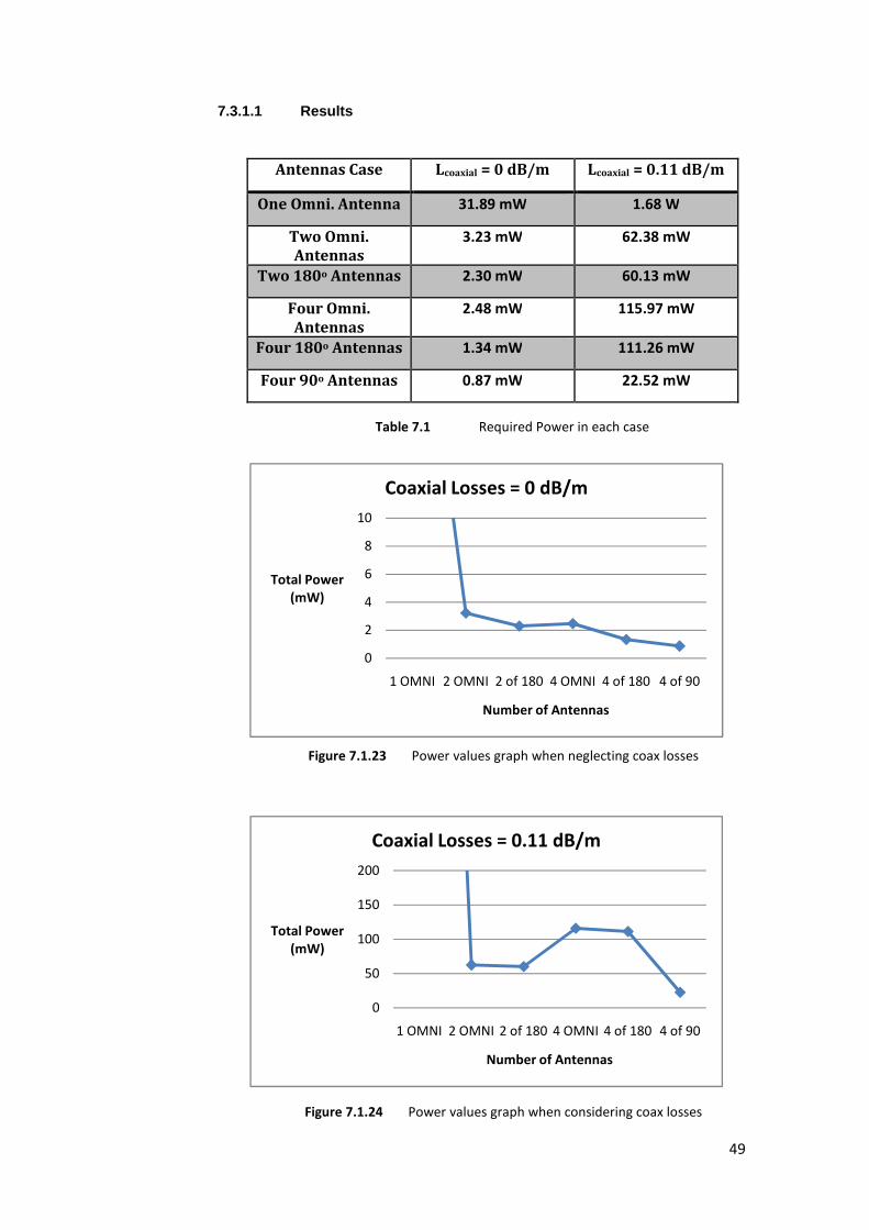
49
7.3.1.1 Results
Antennas Case Lcoaxial = 0 dB/m Lcoaxial = 0.11 dB/m
One Omni. Antenna 31.89 mW 1.68 W
Two Omni.
Antennas
3.23 mW 62.38 mW
Two 180o Antennas 2.30 mW 60.13 mW
Four Omni.
Antennas
2.48 mW 115.97 mW
Four 180o Antennas 1.34 mW 111.26 mW
Four 90o Antennas 0.87 mW 22.52 mW
Table 7.1 Required Power in each case
0
2
4
6
8
10
1 OMNI 2 OMNI 2 of 180 4 OMNI 4 of 180 4 of 90
Total Power
(mW)
Number of Antennas
Coaxial Losses = 0 dB/m
0
50
100
150
200
1 OMNI 2 OMNI 2 of 180 4 OMNI 4 of 180 4 of 90
Total Power
(mW)
Number of Antennas
Coaxial Losses = 0.11 dB/m
Figure 7.1.23 Power values graph when neglecting coax losses
Figure 7.1.24 Power values graph when considering coax losses
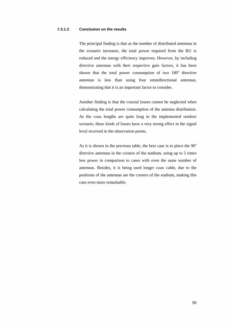
50
7.3.1.2 Conclusion on the results
The principal finding is that as the number of distributed antennas in
the scenario increases, the total power required from the RU is
reduced and the energy efficiency improves. However, by including
directive antennas with their respective gain factors, it has been
shown that the total power consumption of two 180o directive
antennas is less than using four omnidirectional antennas,
demonstrating that it is an important factor to consider.
Another finding is that the coaxial losses cannot be neglected when
calculating the total power consumption of the antenna distribution.
As the coax lengths are quite long in the implemented outdoor
scenario, these kinds of losses have a very strong effect in the signal
level received in the observation points.
As it is shown in the previous table, the best case is to place the 90o
directive antennas in the corners of the stadium, using up to 5 times
less power in comparison to cases with even the same number of
antennas. Besides, it is being used longer coax cable, due to the
positions of the antennas are the corners of the stadium, making this
case even more remarkable.
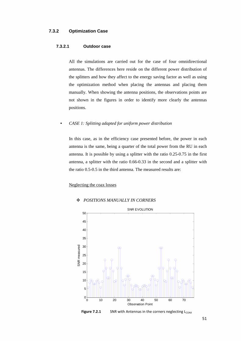
51
7.3.2 Optimization Case
7.3.2.1 Outdoor case
All the simulations are carried out for the case of four omnidirectional
antennas. The differences here reside on the different power distribution of
the splitters and how they affect to the energy saving factor as well as using
the optimization method when placing the antennas and placing them
manually. When showing the antenna positions, the observations points are
not shown in the figures in order to identify more clearly the antennas
positions.
• CASE 1: Splitting adapted for uniform power distribution
In this case, as in the efficiency case presented before, the power in each
antenna is the same, being a quarter of the total power from the RU in each
antenna. It is possible by using a splitter with the ratio 0.25-0.75 in the first
antenna, a splitter with the ratio 0.66-0.33 in the second and a splitter with
the ratio 0.5-0.5 in the third antenna. The measured results are:
Neglecting the coax losses
� POSITIONS MANUALLY IN CORNERS
0 10 20 30 40 50 60 700
5
10
15
20
25
30
35
40
45
50SNR EVOLUTION
Observation Point
SN
R m
easu
red
Figure 7.2.1 SNR with Antennas in the corners neglecting LCOAX
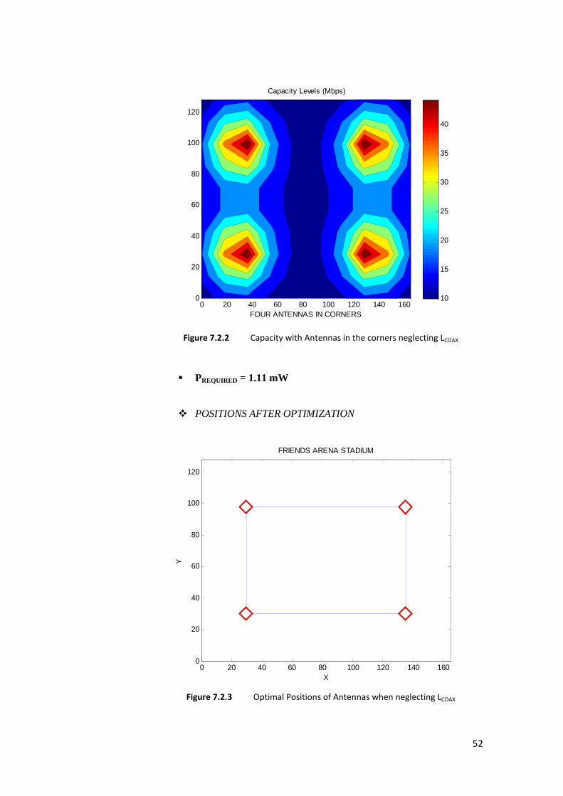
52
� PREQUIRED = 1.11 mW
� POSITIONS AFTER OPTIMIZATION
FOUR ANTENNAS IN CORNERS
Capacity Levels (Mbps)
0 20 40 60 80 100 120 140 1600
20
40
60
80
100
120
10
15
20
25
30
35
40
0 20 40 60 80 100 120 140 1600
20
40
60
80
100
120
FRIENDS ARENA STADIUM
X
Y
Figure 7.2.2 Capacity with Antennas in the corners neglecting LCOAX
Figure 7.2.3 Optimal Positions of Antennas when neglecting LCOAX
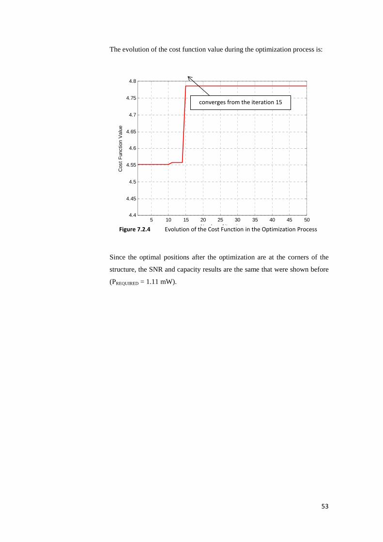
53
The evolution of the cost function value during the optimization process is:
Since the optimal positions after the optimization are at the corners of the
structure, the SNR and capacity results are the same that were shown before
(PREQUIRED = 1.11 mW).
5 10 15 20 25 30 35 40 45 504.4
4.45
4.5
4.55
4.6
4.65
4.7
4.75
4.8
Number of iterarion
Cos
t F
unct
ion
Val
ue
Figure 7.2.4 Evolution of the Cost Function in the Optimization Process
converges from the iteration 15
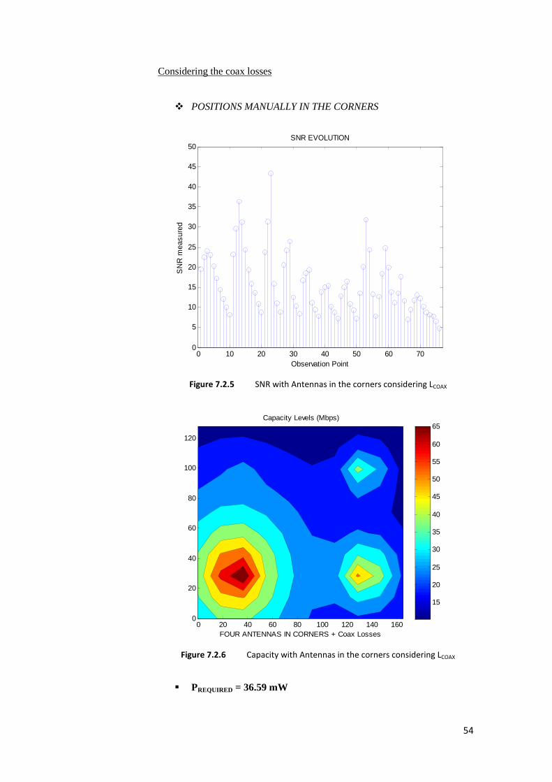
54
Considering the coax losses
� POSITIONS MANUALLY IN THE CORNERS
� PREQUIRED = 36.59 mW
0 10 20 30 40 50 60 700
5
10
15
20
25
30
35
40
45
50SNR EVOLUTION
Observation Point
SN
R m
easu
red
FOUR ANTENNAS IN CORNERS + Coax Losses
Capacity Levels (Mbps)
0 20 40 60 80 100 120 140 1600
20
40
60
80
100
120
15
20
25
30
35
40
45
50
55
60
65
Figure 7.2.5 SNR with Antennas in the corners considering LCOAX
Figure 7.2.6 Capacity with Antennas in the corners considering LCOAX
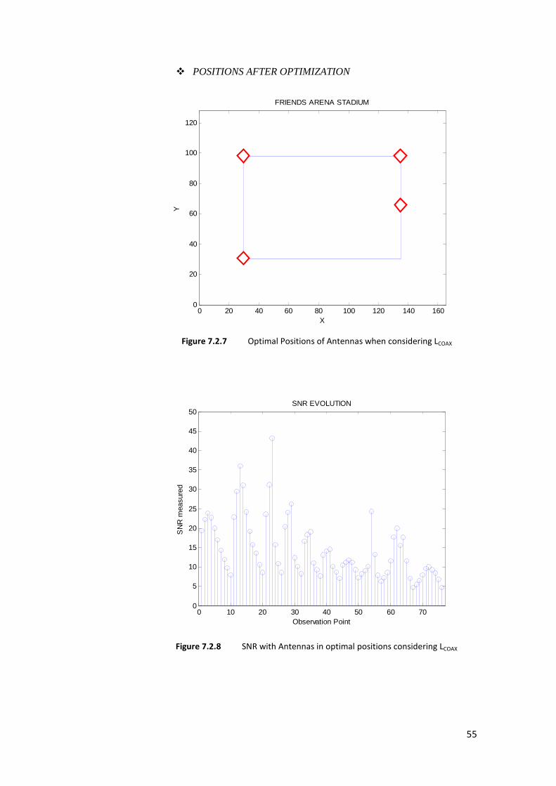
55
� POSITIONS AFTER OPTIMIZATION
0 20 40 60 80 100 120 140 1600
20
40
60
80
100
120
FRIENDS ARENA STADIUM
X
Y
0 10 20 30 40 50 60 700
5
10
15
20
25
30
35
40
45
50SNR EVOLUTION
Observation Point
SN
R m
easu
red
Figure 7.2.7 Optimal Positions of Antennas when considering LCOAX
Figure 7.2.8 SNR with Antennas in optimal positions considering LCOAX
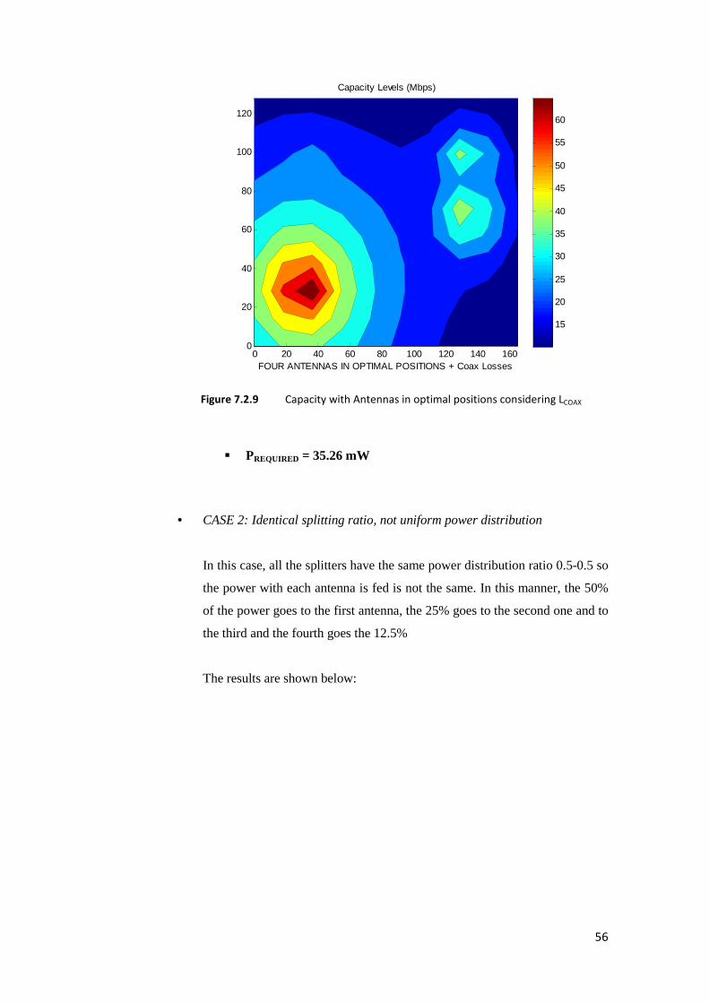
56
� PREQUIRED = 35.26 mW
• CASE 2: Identical splitting ratio, not uniform power distribution
In this case, all the splitters have the same power distribution ratio 0.5-0.5 so
the power with each antenna is fed is not the same. In this manner, the 50%
of the power goes to the first antenna, the 25% goes to the second one and to
the third and the fourth goes the 12.5%
The results are shown below:
FOUR ANTENNAS IN OPTIMAL POSITIONS + Coax Losses
Capacity Levels (Mbps)
0 20 40 60 80 100 120 140 1600
20
40
60
80
100
120
15
20
25
30
35
40
45
50
55
60
Figure 7.2.9 Capacity with Antennas in optimal positions considering LCOAX
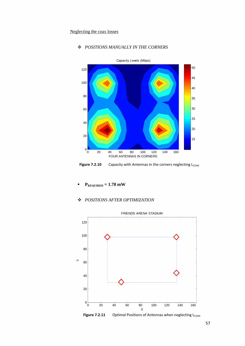
57
Neglecting the coax losses
� POSITIONS MANUALLY IN THE CORNERS
� PREQUIRED = 1.78 mW
� POSITIONS AFTER OPTIMIZATION
FOUR ANTENNAS IN CORNERS
Capacity Levels (Mbps)
0 20 40 60 80 100 120 140 1600
20
40
60
80
100
120
15
20
25
30
35
40
45
50
0 20 40 60 80 100 120 140 1600
20
40
60
80
100
120
FRIENDS ARENA STADIUM
X
Y
Figure 7.2.10 Capacity with Antennas in the corners neglecting LCOAX
Figure 7.2.11 Optimal Positions of Antennas when neglecting LCOAX
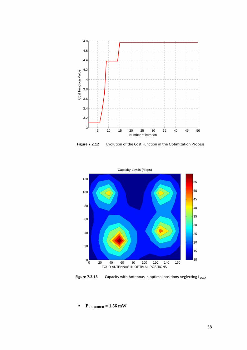
58
� PREQUIRED = 1.56 mW
FOUR ANTENNAS IN OPTIMAL POSITIONS
Capacity Levels (Mbps)
0 20 40 60 80 100 120 140 1600
20
40
60
80
100
120
10
15
20
25
30
35
40
45
50
55
5 10 15 20 25 30 35 40 45 503
3.2
3.4
3.6
3.8
4
4.2
4.4
4.6
4.8
Number of iterarion
Cos
t F
unct
ion
Val
ue
Figure 7.2.13 Capacity with Antennas in optimal positions neglecting LCOAX
Figure 7.2.12 Evolution of the Cost Function in the Optimization Process
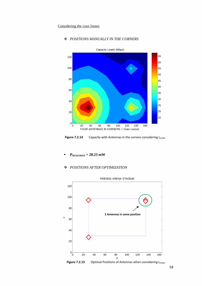
59
Considering the coax losses
� POSITIONS MANUALLY IN THE CORNERS
� PREQUIRED = 28.23 mW
� POSITIONS AFTER OPTIMIZATION
FOUR ANTENNAS IN CORNERS + Coax Losses
Capacity Levels (Mbps)
0 20 40 60 80 100 120 140 1600
20
40
60
80
100
120
15
20
25
30
35
40
45
50
55
60
65
0 20 40 60 80 100 120 140 1600
20
40
60
80
100
120
FRIENDS ARENA STADIUM
X
Y
Figure 7.2.14 Capacity with Antennas in the corners considering LCOAX
Figure 7.2.15 Optimal Positions of Antennas when considering LCOAX
2 Antennas in same position
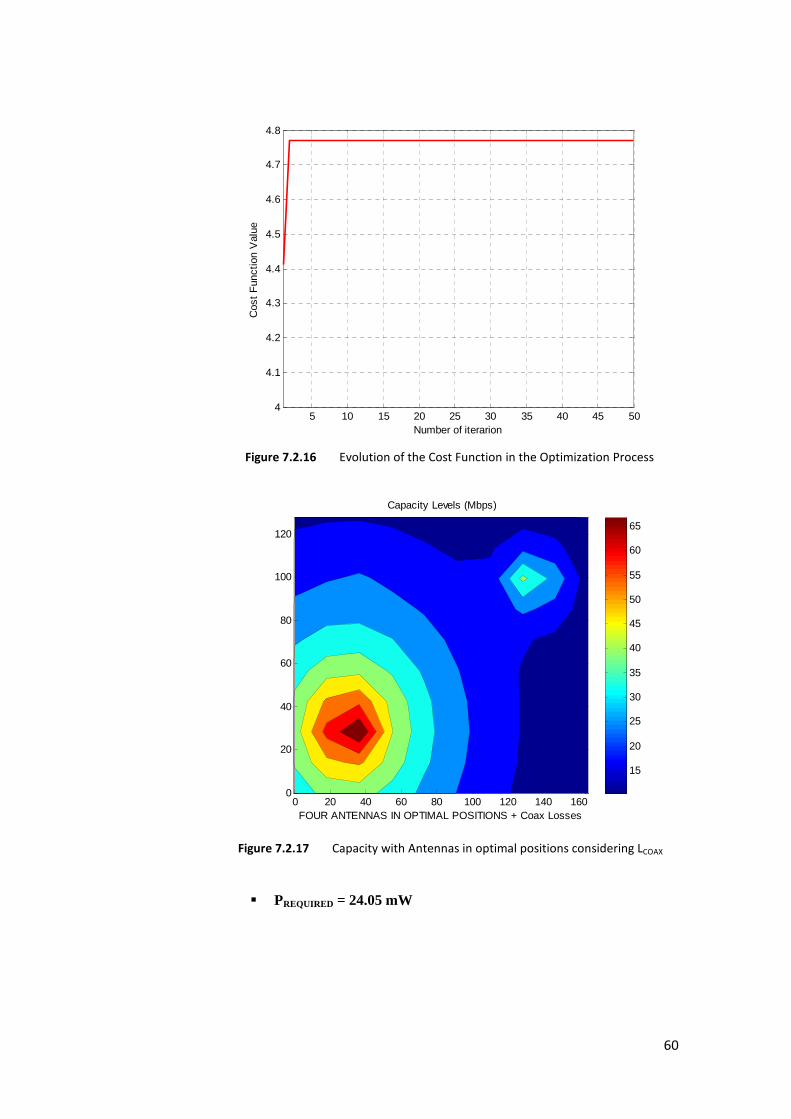
60
FOUR ANTENNAS IN OPTIMAL POSITIONS + Coax Losses
Capacity Levels (Mbps)
0 20 40 60 80 100 120 140 1600
20
40
60
80
100
120
15
20
25
30
35
40
45
50
55
60
65
� PREQUIRED = 24.05 mW
5 10 15 20 25 30 35 40 45 504
4.1
4.2
4.3
4.4
4.5
4.6
4.7
4.8
Number of iterarion
Cos
t F
unct
ion
Val
ue
Figure 7.2.17 Capacity with Antennas in optimal positions considering LCOAX
Figure 7.2.16 Evolution of the Cost Function in the Optimization Process
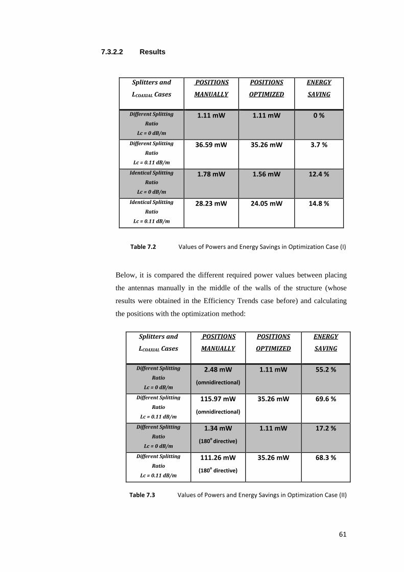
61
7.3.2.2 Results
Splitters and
LCOAXIAL Cases
POSITIONS
MANUALLY
POSITIONS
OPTIMIZED
ENERGY
SAVING
Different Splitting
Ratio
Lc = 0 dB/m
1.11 mW 1.11 mW 0 %
Different Splitting
Ratio
Lc = 0.11 dB/m
36.59 mW 35.26 mW 3.7 %
Identical Splitting
Ratio
Lc = 0 dB/m
1.78 mW 1.56 mW 12.4 %
Identical Splitting
Ratio
Lc = 0.11 dB/m
28.23 mW 24.05 mW 14.8 %
Table 7.2 Values of Powers and Energy Savings in Optimization Case (I)
Below, it is compared the different required power values between placing
the antennas manually in the middle of the walls of the structure (whose
results were obtained in the Efficiency Trends case before) and calculating
the positions with the optimization method:
Splitters and
LCOAXIAL Cases
POSITIONS
MANUALLY
POSITIONS
OPTIMIZED
ENERGY
SAVING
Different Splitting
Ratio
Lc = 0 dB/m
2.48 mW
(omnidirectional)
1.11 mW 55.2 %
Different Splitting
Ratio
Lc = 0.11 dB/m
115.97 mW
(omnidirectional)
35.26 mW 69.6 %
Different Splitting
Ratio
Lc = 0 dB/m
1.34 mW
(180o
directive)
1.11 mW 17.2 %
Different Splitting
Ratio
Lc = 0.11 dB/m
111.26 mW
(180o directive)
35.26 mW 68.3 %
Table 7.3 Values of Powers and Energy Savings in Optimization Case (II)
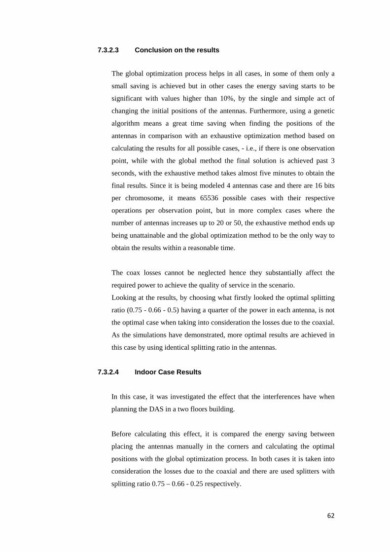
62
7.3.2.3 Conclusion on the results
The global optimization process helps in all cases, in some of them only a
small saving is achieved but in other cases the energy saving starts to be
significant with values higher than 10%, by the single and simple act of
changing the initial positions of the antennas. Furthermore, using a genetic
algorithm means a great time saving when finding the positions of the
antennas in comparison with an exhaustive optimization method based on
calculating the results for all possible cases, - i.e., if there is one observation
point, while with the global method the final solution is achieved past 3
seconds, with the exhaustive method takes almost five minutes to obtain the
final results. Since it is being modeled 4 antennas case and there are 16 bits
per chromosome, it means 65536 possible cases with their respective
operations per observation point, but in more complex cases where the
number of antennas increases up to 20 or 50, the exhaustive method ends up
being unattainable and the global optimization method to be the only way to
obtain the results within a reasonable time.
The coax losses cannot be neglected hence they substantially affect the
required power to achieve the quality of service in the scenario.
Looking at the results, by choosing what firstly looked the optimal splitting
ratio (0.75 - 0.66 - 0.5) having a quarter of the power in each antenna, is not
the optimal case when taking into consideration the losses due to the coaxial.
As the simulations have demonstrated, more optimal results are achieved in
this case by using identical splitting ratio in the antennas.
7.3.2.4 Indoor Case Results
In this case, it was investigated the effect that the interferences have when
planning the DAS in a two floors building.
Before calculating this effect, it is compared the energy saving between
placing the antennas manually in the corners and calculating the optimal
positions with the global optimization process. In both cases it is taken into
consideration the losses due to the coaxial and there are used splitters with
splitting ratio 0.75 – 0.66 - 0.25 respectively.
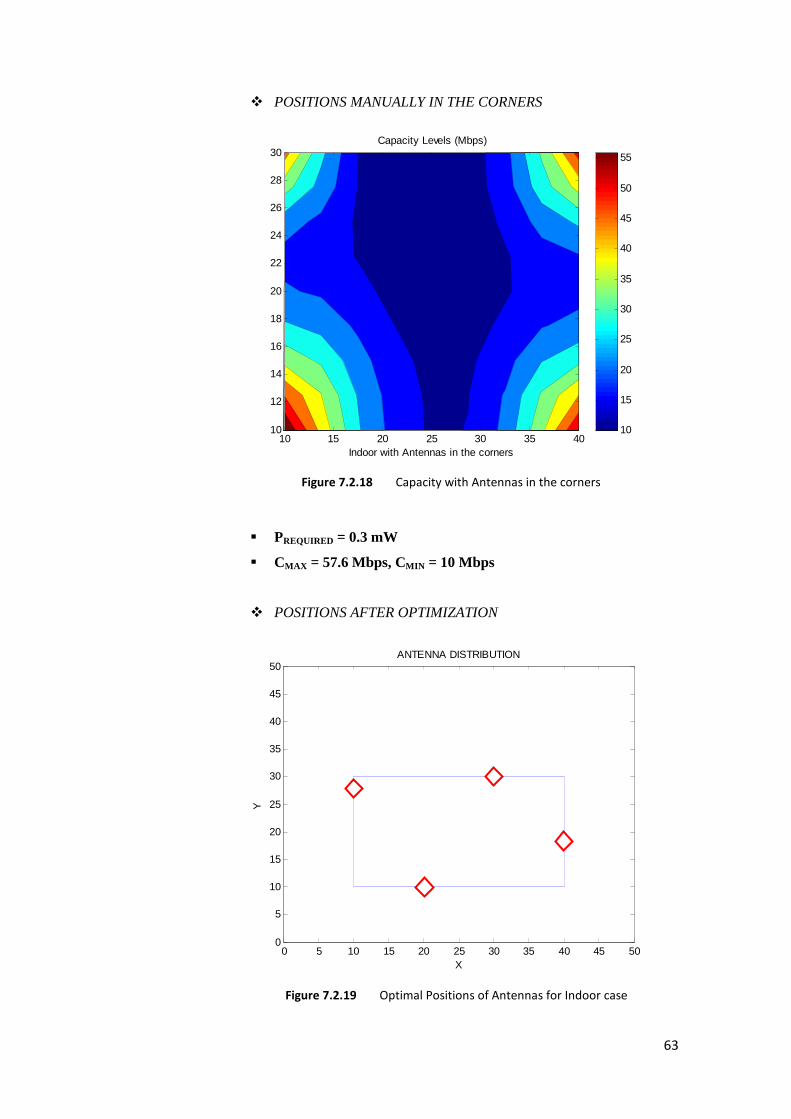
63
Indoor with Antennas in the corners
Capacity Levels (Mbps)
10 15 20 25 30 35 4010
12
14
16
18
20
22
24
26
28
30
10
15
20
25
30
35
40
45
50
55
� POSITIONS MANUALLY IN THE CORNERS
Figure 7.2.18 Capacity with Antennas in the corners
� PREQUIRED = 0.3 mW
� CMAX = 57.6 Mbps, CMIN = 10 Mbps
� POSITIONS AFTER OPTIMIZATION
0 5 10 15 20 25 30 35 40 45 500
5
10
15
20
25
30
35
40
45
50ANTENNA DISTRIBUTION
X
Y
Figure 7.2.19 Optimal Positions of Antennas for Indoor case
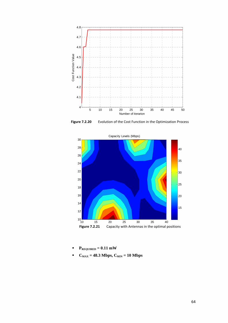
64
� PREQUIRED = 0.11 mW
� CMAX = 48.3 Mbps, CMIN = 10 Mbps
1st FLOOR WITHOUT 2nd FLOOR EFFECT
Capacity Levels (Mbps)
10 15 20 25 30 35 4010
12
14
16
18
20
22
24
26
28
30
15
20
25
30
35
40
5 10 15 20 25 30 35 40 45 504
4.1
4.2
4.3
4.4
4.5
4.6
4.7
4.8
Number of iterarion
Cos
t F
unct
ion
Val
ue
Figure 7.2.21 Capacity with Antennas in the optimal positions
Figure 7.2.20 Evolution of the Cost Function in the Optimization Process
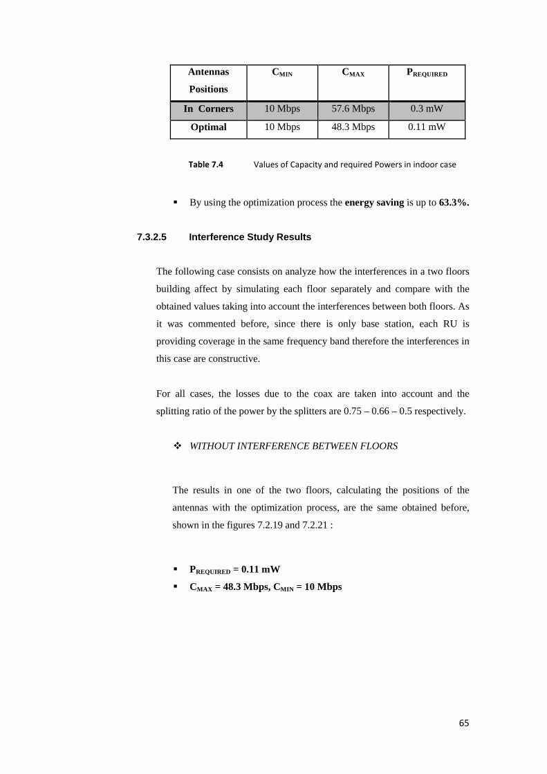
65
Antennas
Positions
CMIN CMAX PREQUIRED
In Corners 10 Mbps 57.6 Mbps 0.3 mW
Optimal 10 Mbps 48.3 Mbps 0.11 mW
Table 7.4 Values of Capacity and required Powers in indoor case
� By using the optimization process the energy saving is up to 63.3%.
7.3.2.5 Interference Study Results
The following case consists on analyze how the interferences in a two floors
building affect by simulating each floor separately and compare with the
obtained values taking into account the interferences between both floors. As
it was commented before, since there is only base station, each RU is
providing coverage in the same frequency band therefore the interferences in
this case are constructive.
For all cases, the losses due to the coax are taken into account and the
splitting ratio of the power by the splitters are 0.75 – 0.66 – 0.5 respectively.
� WITHOUT INTERFERENCE BETWEEN FLOORS
The results in one of the two floors, calculating the positions of the
antennas with the optimization process, are the same obtained before,
shown in the figures 7.2.19 and 7.2.21 :
� PREQUIRED = 0.11 mW
� CMAX = 48.3 Mbps, CMIN = 10 Mbps
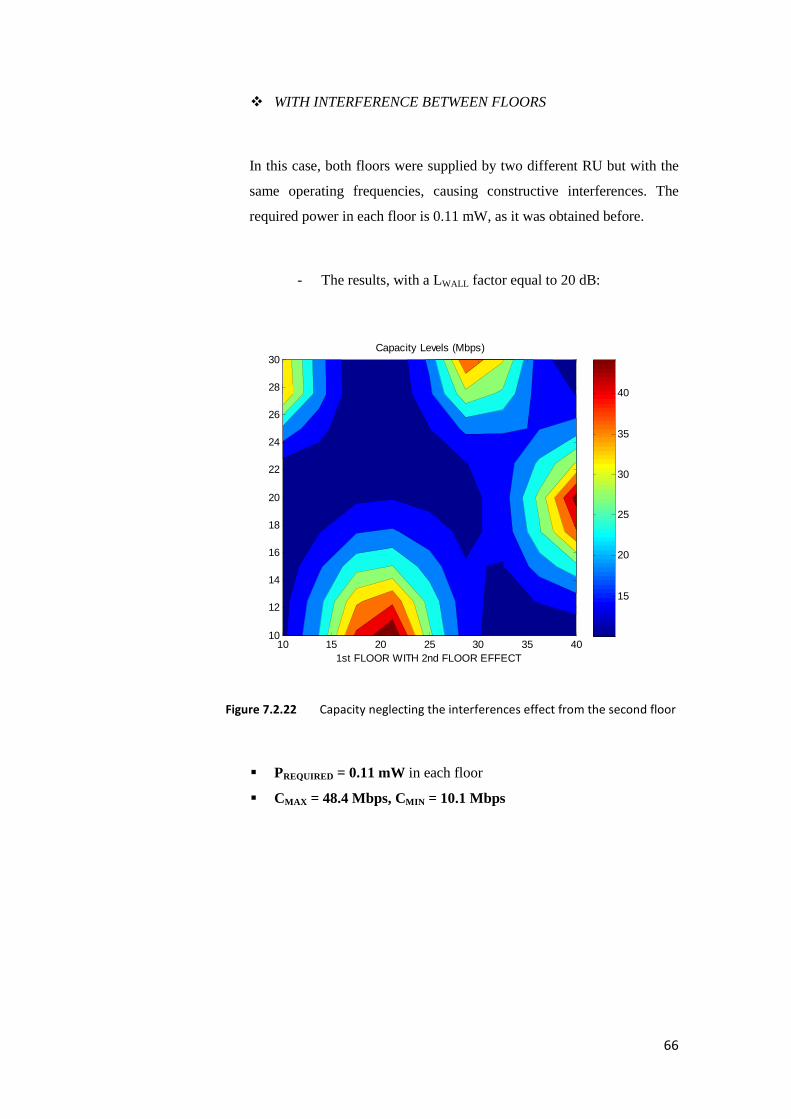
66
� WITH INTERFERENCE BETWEEN FLOORS
In this case, both floors were supplied by two different RU but with the
same operating frequencies, causing constructive interferences. The
required power in each floor is 0.11 mW, as it was obtained before.
- The results, with a LWALL factor equal to 20 dB:
� PREQUIRED = 0.11 mW in each floor
� CMAX = 48.4 Mbps, CMIN = 10.1 Mbps
1st FLOOR WITH 2nd FLOOR EFFECT
Capacity Levels (Mbps)
10 15 20 25 30 35 4010
12
14
16
18
20
22
24
26
28
30
15
20
25
30
35
40
Figure 7.2.22 Capacity neglecting the interferences effect from the second floor
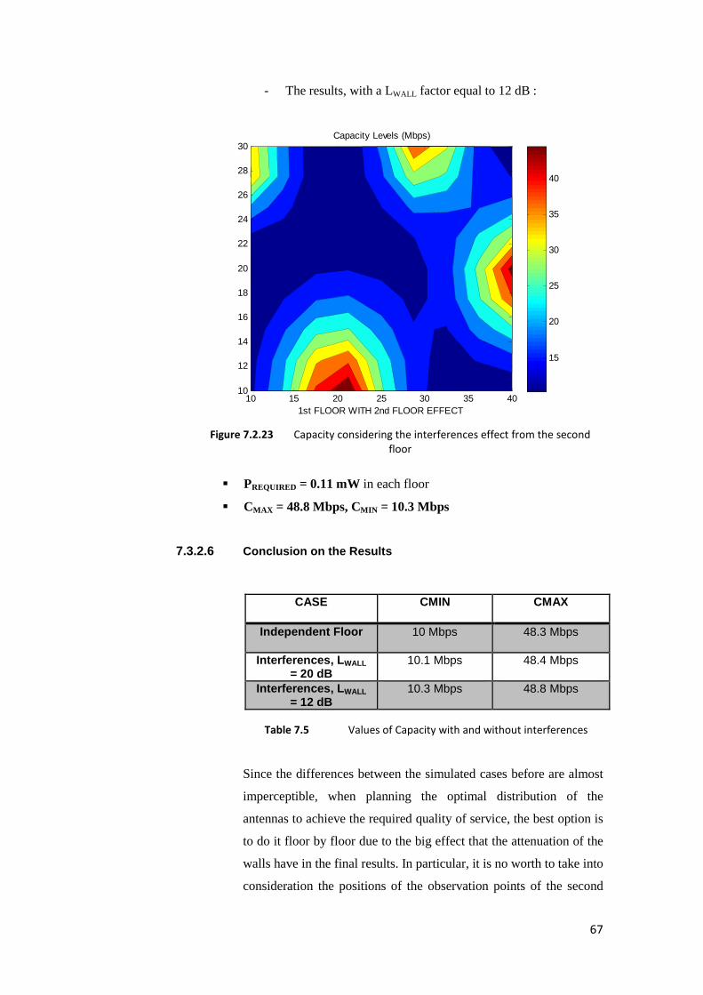
67
- The results, with a LWALL factor equal to 12 dB :
� PREQUIRED = 0.11 mW in each floor
� CMAX = 48.8 Mbps, CMIN = 10.3 Mbps
7.3.2.6 Conclusion on the Results
Since the differences between the simulated cases before are almost
imperceptible, when planning the optimal distribution of the
antennas to achieve the required quality of service, the best option is
to do it floor by floor due to the big effect that the attenuation of the
walls have in the final results. In particular, it is no worth to take into
consideration the positions of the observation points of the second
CASE
CMIN CMAX
Independent Floor
10 Mbps 48.3 Mbps
Interferences, L WALL = 20 dB
10.1 Mbps 48.4 Mbps
Interferences, L WALL = 12 dB
10.3 Mbps 48.8 Mbps
Table 7.5 Values of Capacity with and without interferences
1st FLOOR WITH 2nd FLOOR EFFECT
Capacity Levels (Mbps)
10 15 20 25 30 35 4010
12
14
16
18
20
22
24
26
28
30
15
20
25
30
35
40
Figure 7.2.23 Capacity considering the interferences effect from the second
floor
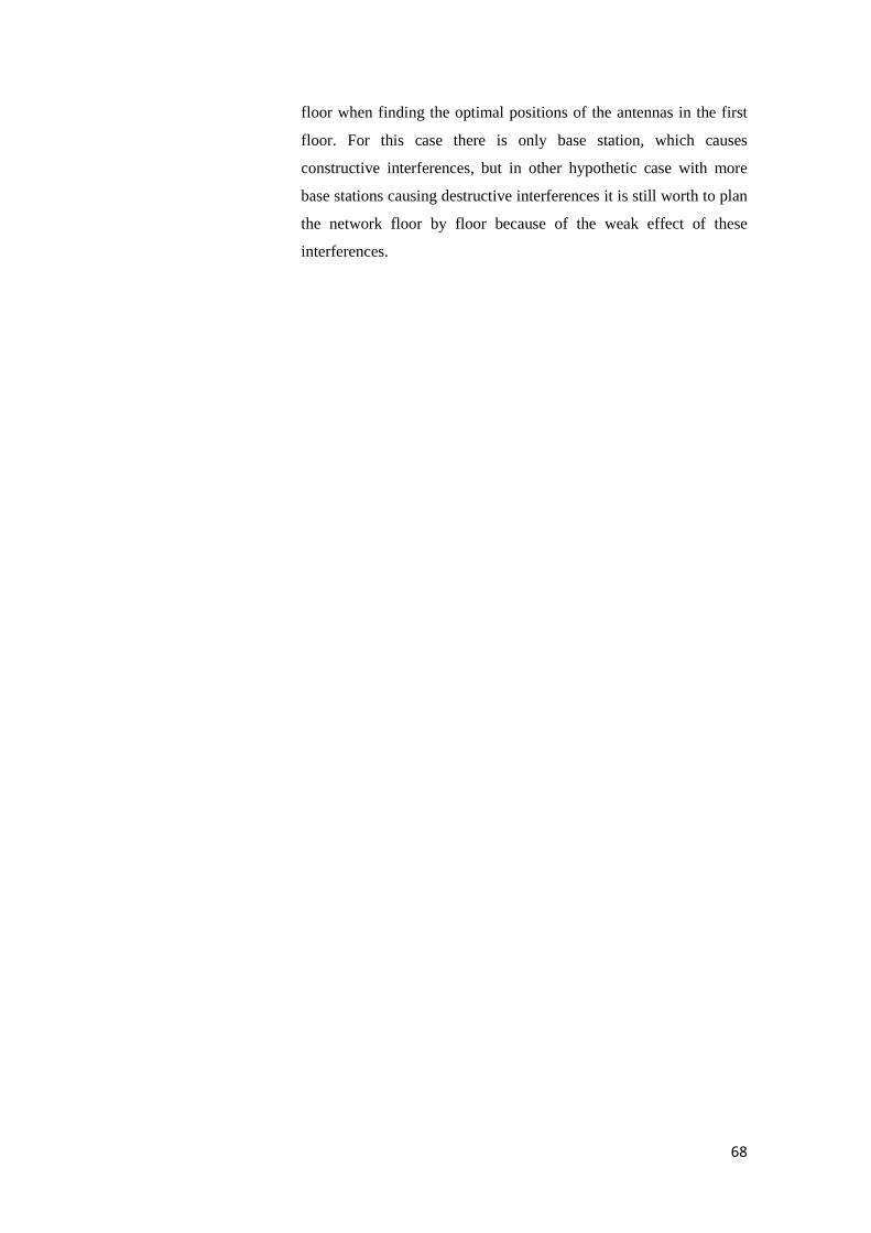
68
floor when finding the optimal positions of the antennas in the first
floor. For this case there is only base station, which causes
constructive interferences, but in other hypothetic case with more
base stations causing destructive interferences it is still worth to plan
the network floor by floor because of the weak effect of these
interferences.
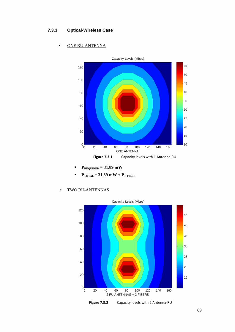
69
7.3.3 Optical-Wireless Case
• ONE RU-ANTENNA
� PREQUIRED = 31.89 mW
� PTOTAL = 31.89 mW + P1_FIBER
• TWO RU-ANTENNAS
ONE ANTENNA
Capacity Levels (Mbps)
0 20 40 60 80 100 120 140 1600
20
40
60
80
100
120
10
15
20
25
30
35
40
45
50
55
2 RU-ANTENNAS + 2 FIBERS
Capacity Levels (Mbps)
0 20 40 60 80 100 120 140 1600
20
40
60
80
100
120
15
20
25
30
35
40
45
Figure 7.3.1 Capacity levels with 1 Antenna-RU
Figure 7.3.2 Capacity levels with 2 Antenna-RU
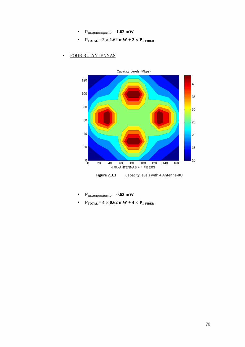
70
� PREQUIREDperRU = 1.62 mW
� PTOTAL = 2×1.62 mW + 2×P1_FIBER
• FOUR RU-ANTENNAS
� PREQUIREDperRU = 0.62 mW
� PTOTAL = 4×0.62 mW + 4×P1_FIBER
4 RU-ANTENNAS + 4 FIBERS
Capacity Levels (Mbps)
0 20 40 60 80 100 120 140 1600
20
40
60
80
100
120
10
15
20
25
30
35
40
Figure 7.3.3 Capacity levels with 4 Antenna-RU
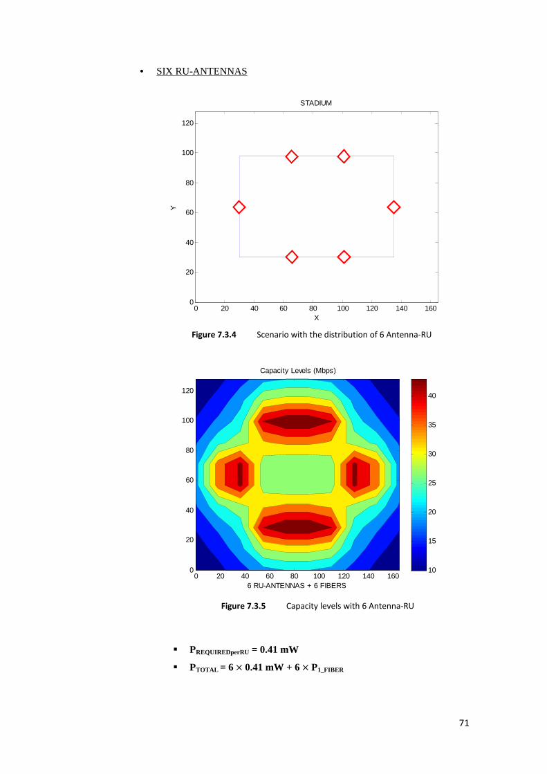
71
• SIX RU-ANTENNAS
� PREQUIREDperRU = 0.41 mW
� PTOTAL = 6×0.41 mW + 6×P1_FIBER
0 20 40 60 80 100 120 140 1600
20
40
60
80
100
120
STADIUM
X
Y
6 RU-ANTENNAS + 6 FIBERS
Capacity Levels (Mbps)
0 20 40 60 80 100 120 140 1600
20
40
60
80
100
120
10
15
20
25
30
35
40
Figure 7.3.4 Scenario with the distribution of 6 Antenna-RU
Figure 7.3.5 Capacity levels with 6 Antenna-RU
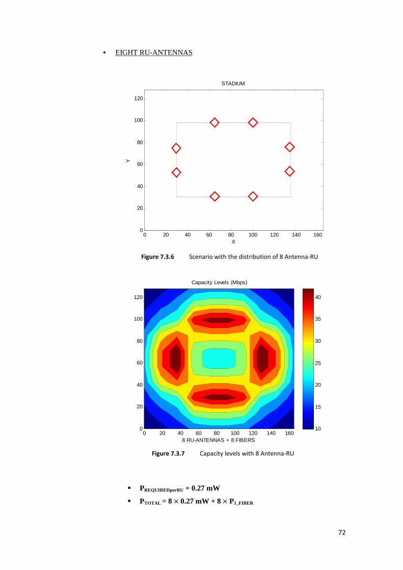
72
• EIGHT RU-ANTENNAS
� PREQUIREDperRU = 0.27 mW
� PTOTAL = 8×0.27 mW + 8×P1_FIBER
0 20 40 60 80 100 120 140 1600
20
40
60
80
100
120
STADIUM
X
Y
8 RU-ANTENNAS + 8 FIBERS
Capacity Levels (Mbps)
0 20 40 60 80 100 120 140 1600
20
40
60
80
100
120
10
15
20
25
30
35
40
Figure 7.3.6 Scenario with the distribution of 8 Antenna-RU
Figure 7.3.7 Capacity levels with 8 Antenna-RU
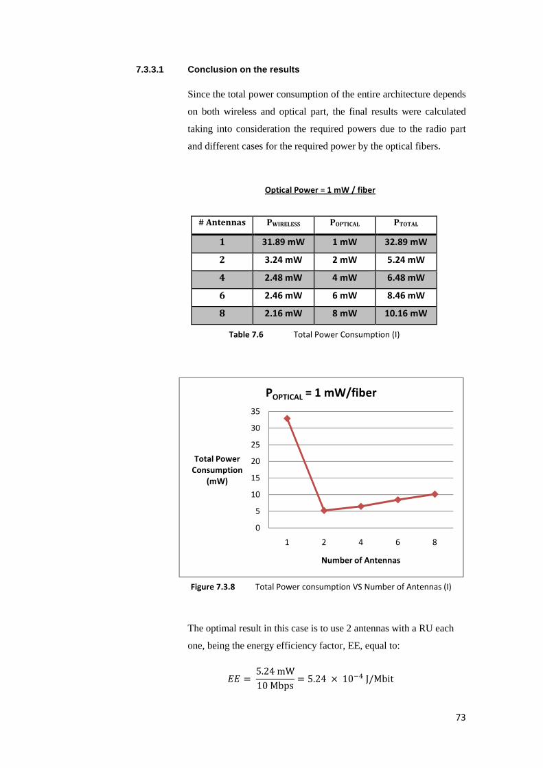
73
7.3.3.1 Conclusion on the results Since the total power consumption of the entire architecture depends
on both wireless and optical part, the final results were calculated
taking into consideration the required powers due to the radio part
and different cases for the required power by the optical fibers.
Optical Power = 1 mW / fiber
The optimal result in this case is to use 2 antennas with a RU each
one, being the energy efficiency factor, EE, equal to:
@@ =5.24mW10Mbps = 5.24 ×10&vJ/Mbit
# Antennas PWIRELESS POPTICAL PTOTAL
1 31.89 mW 1 mW 32.89 mW
2 3.24 mW 2 mW 5.24 mW
4 2.48 mW 4 mW 6.48 mW
6 2.46 mW 6 mW 8.46 mW
8 2.16 mW 8 mW 10.16 mW
Table 7.6 Total Power Consumption (I)
0
5
10
15
20
25
30
35
1 2 4 6 8
Total Power
Consumption
(mW)
Number of Antennas
POPTICAL = 1 mW/fiber
Figure 7.3.8 Total Power consumption VS Number of Antennas (I)
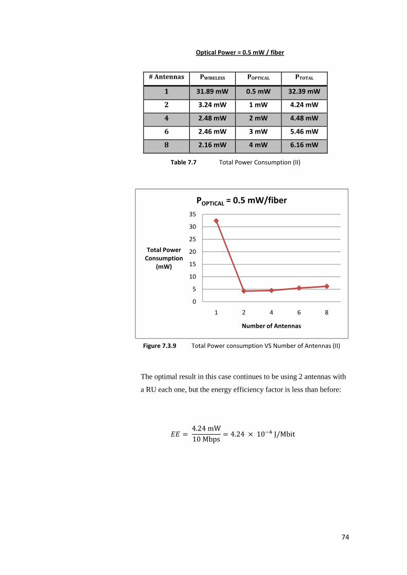
74
Optical Power = 0.5 mW / fiber
The optimal result in this case continues to be using 2 antennas with
a RU each one, but the energy efficiency factor is less than before:
@@ =4.24mW10Mbps = 4.24 ×10&vJ/Mbit
# Antennas PWIRELESS POPTICAL PTOTAL
1 31.89 mW 0.5 mW 32.39 mW
2 3.24 mW 1 mW 4.24 mW
4 2.48 mW 2 mW 4.48 mW
6 2.46 mW 3 mW 5.46 mW
8 2.16 mW 4 mW 6.16 mW
Table 7.7 Total Power Consumption (II)
0
5
10
15
20
25
30
35
1 2 4 6 8
Total Power
Consumption
(mW)
Number of Antennas
POPTICAL = 0.5 mW/fiber
Figure 7.3.9 Total Power consumption VS Number of Antennas (II)
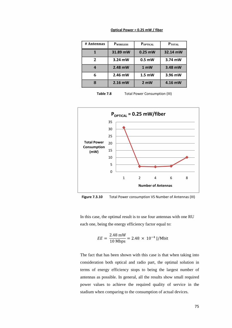
75
Optical Power = 0.25 mW / fiber
In this case, the optimal result is to use four antennas with one RU
each one, being the energy efficiency factor equal to:
@@ =2.48mW10Mbps = 2.48 ×10&vJ/Mbit
The fact that has been shown with this case is that when taking into
consideration both optical and radio part, the optimal solution in
terms of energy efficiency stops to being the largest number of
antennas as possible. In general, all the results show small required
power values to achieve the required quality of service in the
stadium when comparing to the consumption of actual devices.
# Antennas PWIRELESS POPTICAL PTOTAL
1 31.89 mW 0.25 mW 32.14 mW
2 3.24 mW 0.5 mW 3.74 mW
4 2.48 mW 1 mW 3.48 mW
6 2.46 mW 1.5 mW 3.96 mW
8 2.16 mW 2 mW 4.16 mW
Table 7.8 Total Power Consumption (III)
0
5
10
15
20
25
30
35
1 2 4 6 8
Total Power
Consumption
(mW)
Number of Antennas
POPTICAL = 0.25 mW/fiber
Figure 7.3.10 Total Power consumption VS Number of Antennas (III)
76
Chapter 8 Conclusion and Future Work
During the different steps carried out in the project it has been shown that the quality of
service can be retained meanwhile achieving an energy saving, in other words, by using
less power to assure the required QoS and, conversely by using the same power obtain a
better QoS.
Taking into account only the radio part may suggest that the more antennas are used the
better the energy efficiency. However, by taking into account both the optical and radio
power consumption can set up an upper bound for energy efficiency, and the optimal
balance between the number of nodes and the total power needed will vary depending
on both optical and radio parts. It is worth to remind that the actual radiated power
required to achieve, in particular for our studies, 10 Mb/s in the stadium is in the order
of mW, whereas the consumption of actual devices can be 100 or even 1000 time larger.
It means that there is a substantial room for improvement, in terms of energy
consumption, for the current equipment.
When designing a distributed antenna network system it is important not to ignore the
following factors: the losses due to the coax cable, the directivity and gain factors of the
antennas or the power splitting ratio of the splitters play an important role in the final
results.
The use of the global optimization has resulted to be an efficient tool when planning the
positions of the antennas in terms of time and energy saving. In this case, the resolution
of each parameter was 4 bits, but a future improvement could be to upgrade the
resolution by increasing the number of bits per parameter. Furthermore, the
optimization process could be also responsible for calculating the optimal number of the
antennas depending on the specific scenario and environment.
The simulations are implemented under the assumption that there is only one base
station used with the DAS. One of the future developments of the model is to
implement the multi-BS case. In this case, there will be necessary to consider that in the
same scenario, different antenna systems are emitting in different frequency bands. The
interferences, both constructive and destructive, will play an important role when
looking for the optimal planning for such a multi-base station case in terms of energy
efficiency.
77
Finally, one of the most interesting developments in a future model is to create and test
a model for Dynamic Capacity Allocation. It consists of a smarter DAS architecture that
will dynamically regulate the capacity depending on the conditions to which the
scenario is exposed: enable/disable RU, use same/different coverage frequencies or
increase/decrease required power by differentiating, for example, when the stadium is
full of people or not, when it is being used for a sport event or for a concert when the
people are not allocated in the same places, if it is a day or night event, etc.
Any improvement in the implemented models will be welcome since those upgrades
have been found for the benefit of something such important as the energy efficiency.
78
References
[1] Website: < http://www.gsmworld.com/about/history.shtml >, last visited February 2013.
[2] M.Tolstrup. “Indoor Radio Planning: A practical guide for GSM, DCS, UMTS and HSPA”,
Wiley, 2008.
[3] J.Laiho, A.Wacker, T.Novosad. “Radio Network Planning and Optimization for UMTS”,
Wiley, 2006.
[4] A.Ali Bajwa. “Investigation on Radiation Conditions using Active DAS compared to
Passive DAS”, Master of Science Thesis, 2008.
[5] Y.Josse, B.Fracasso, P.Pajusco. “Model for energy efficiency in radio over fiber
distributed indoor antenna Wi-Fi network”, The 14th International Symposium on Wireless
Personal Multimedia Communications, 2011.
[6] Green DAS project, https://www.acreo.se/Green-DAS , May 2013.
[7] S.R.Saunders. “Antennas and Propagation for Wireless Communication Systems”, Wiley,
1999.
[8] E. Semaan, “Operator Diversity in Forest and Rural Applications”, Master of Science
Thesis, 2011.
[9] L.Ahlin, J.Zander, B.Slimane. “Principles of Wireless Communications”, Studenlitteratur,
2006.
[10] Website: < https://www.classle.net/book/shannon-limit-information-capacity >, last visited
May 2013
[11] N.Shabbir, H. Kashif. “Radio Resource Management in WiMax”, Master of Science in
Electrical Engineering, 2009
79
[12] D.Tipper. “UMTS Overview”, Graduate Telecommunications and Networking Program,
University of Pittsburgh, available at
<http://www.sis.pitt.edu/~dtipper/2720/2720_Slides12.pdf>, last visited May 2013.
[13] Website: < http://friendsarena.se/Arenan/ >, last visited May 2013.
[14] Website: < http://www.mathworks.se/products/matlab/ >, last visited May 2013.
[15] M.Popov. “Analytic and Numerical Methods for the Solution of Electromagnetic Inverse
Source Problems”, Division of Electromagnetic Theory Department of Signals, Sensors and
Systems, Royal Institute of Technology, Stockholm, 2001.
[16] J.Michael Johnson, Y. Rahmat-Samii. “Genetic Algorithms in Engineering
Electromagnetics”, IEEE Antennas and Propagation Magazine, Vol. 39, No. 4, August 1997.

80

www.kth.se
TRITA-ICT-EX-2013:97