GREATER SAGE-GROUSE (Centrocercus urophasianus) … · 1 Holloran, Matthew J., Greater Sage-Grouse (Centrocercus urophasianus) Population Response to Natural Gas Field Development

GREATER SAGE-GROUSE (Centrocercus urophasianus) POPULATION RESPONSE TO NATURAL GAS FIELD DEVELOPMENT IN WESTERN WYOMING

by Matthew J. Holloran

A dissertation submitted to the Department of Zoology and Physiology and The Graduate School of The University of Wyoming

in partial fulfillment of the requirements for the degree of

DOCTOR OF PHILOSOPHY in

ZOOLOGY AND PHYSIOLOGY

Laramie, Wyoming December, 2005

To The Graduate School:

The members of the committee approve the dissertation of Matthew J. Holloran presented on

October 20,2005.

Stanley H. Anderson, Chair in Memoriam

Archie F. Reeve

(0 ~WJ C. t:I;Daniel C. Rule

APPROVED:

Graham Mitchell, Head, Department of Zoology and Physiology

Don A. Roth, Dean, The Graduate School

1

Holloran, Matthew J., Greater Sage-Grouse (Centrocercus urophasianus) Population Response to Natural Gas Field Development in Western Wyoming. PhD, Department of Zoology and Physiology, December, 2005.

Sage-grouse (Centrocercus spp.) populations have declined dramatically throughout the western

United States since the 1960s. Increased gas and oil development during this time has potentially

contributed to the declines. I investigated impacts of development of natural gas fields on greater sage-

grouse (C. urophasianus) breeding behavior, seasonal habitat selection, and population growth in the

upper Green River Basin of western Wyoming. Greater sage-grouse in western Wyoming appeared to

be excluded from attending leks situated within or near the development boundaries of natural gas

fields. Declines in the number of displaying males were positively correlated with decreased distance

from leks to gas-field-related sources of disturbance, increased levels of development surrounding leks,

increased traffic volumes within 3 km of leks, and increased potential for greater noise intensity at leks.

Displacement of adult males and low recruitment of juvenile males contributed to declines in the

number of breeding males on impacted leks. Additionally, responses of predatory species to

development of gas fields could be responsible for decreased male survival on leks situated near the

edges of developing fields and could extend the range-of-influence of gas fields. Generally, nesting

females avoided areas with high densities of producing wells, and brooding females avoided producing

wells. However, the relationship between selected nesting sites and proximity to gas field infrastructure

shifted between 2000 – 2003 and 2004, with females selecting nesting habitat farther from active

drilling rigs and producing wells in 2004. This suggests that the long-term response of nesting

populations is avoidance of natural gas development. Most of the variability in population growth

between populations that were impacted and non-impacted by natural gas development was explained

by lower annual survival buffered to some extent by higher productivity in impacted populations.

Seasonal survival differences between impacted and non-impacted individuals indicates that a lag

period occurs between when an individual is impacted by an anthropogenic disturbance and when

survival probabilities are influenced, suggesting negative fitness consequences for females subjected to

natural gas development during the breeding or nesting periods. I suggest that currently imposed

development stipulations are inadequate to protect greater sage-grouse, and that stipulations need to be

modified to maintain populations within natural gas fields.

ii

TABLE OF CONTENTS

Acknowledgments x

Preface 1

Goals and Objectives 2

Dissertation Organization 3

Literature Cited 5

Chapter 1: GREATER SAGE-GROUSE POPULATION RESPONSE TO NATURAL GAS FIELD

DEVELOPMENT IN WESTERN WYOMING: ARE REGIONAL POPULATIONS AFFECTED BY

RELATIVELY LOCALIZED DISTURBANCES?

Introduction 6

Greater Sage-grouse Population Response to Gas Development 8

Are Regional Populations Affected? 10

Concluding Comments 11

Acknowledgments 13

References 13

Chapter 2: GREATER SAGE-GROUSE RESPONSE TO NATURAL GAS FIELD DEVELOPMENT

IN WESTERN WYOMING.

Introduction 16

Study Area 18

Field Methods

Lek Analyses 19

Lek Counts 19

Trapping 19

Male Habitat Selection 19

Female Habitat Selection and Demographic Analyses 20

Female Nesting Habitat Selection 20

Female Brood-rearing Habitat Selection and Productivity 21

Female Annual Survival 21

Female Chick Winter Survival 21

iii

Statistical Methods

Lek Analyses 21

Male Habitat Selection 23

First Level: Initial Determination of Treatment and Control

Leks 24

Second Level: Refinement of Potential Treatment Effect and Within

Treatment Level Influences 25

Drilling Rig 25

Producing Well 26

Main Haul Road 26

Third Level: Inclusive Gas Field Infrastructure Impacts 27

Female Habitat Selection Analyses 28

Consecutive Years’ Nests 29

Adult versus Yearling Nest 30

Used versus Available and Successful versus Unsuccessful Nest

Locations 30

Used versus Available and Successful versus Unsuccessful Early

Brood-rearing Locations 32

Female Demographic Analyses

Vital Rate Estimation 33

Deterministic Analysis 35

Life Table Response Experiment 37

Stochastic Simulations 37

Results

Lek Analyses 38

First Level: Initial Determination of Treatment and Control

Leks 38

Second Level: Refinement of Potential Treatment Effect and Within

Treatment Level Influences

Drilling Rig 39

Producing Well 39

Main Haul Road 40

Third Level: Inclusive Gas Field Infrastructure Impacts 42

iv


Consecutive years’ nests 43

Adult versus Yearling Nest 43

Used versus Available Nests 44

Successful versus Unsuccessful Nests 44

Used versus Available and Successful versus Unsuccessful Early

Brood-rearing Locations 45

Female Demographic Analyses 45

Vital Rate Estimation 45

Deterministic Analysis 47

Life Table Response Experiment 48

Stochastic Simulations 48

Discussion

Lek Analyses 49


Female Demographic Analyses 54

Summary 56

Management Implications 57

Acknowledgements 60

Literature Cited 60

Tables

Table 1. List of acronyms. 68

Table 2. Mean annual declines in the number of greater sage-grouse males attending

leks in western Wyoming, 1998-2004 by the total number of potential natural gas field-

related impacts occurring within specified distances of the lek. 70

Table 3. Mean nest-to-natural gas field related disturbance distances for adult and

yearling greater sage-grouse in western Wyoming, 2000-2004. 71

Table 4. Parameter coefficients for AICc weighted logistic regression models comparing

selected nesting sites and random locations for greater sage-grouse in western Wyoming,

2000-2004. 72

Table 5. Parameter coefficients and cumulative AICc weights for independent variables

included in AICc weighted logistic regression models comparing successful to

unsuccessful nesting sites for greater sage-grouse in western Wyoming,

v

2000-2004. 73

Table 6. Mean distances to natural gas field related disturbances for early brood-rearing

used and available sites, and mean nest-to-disturbance source distances for successful

and unsuccessful brooding greater sage-grouse in western Wyoming,

2000-2004. 74

Table 7. Apparent nest propensity, adjusted nest success probabilities, and brood

survival probabilities for adult and yearling greater sage-grouse females in southwestern

Wyoming, 1998-2004. 75

Table 8. Investigation of year, age and breeding status effect on annual survival of

greater sage-grouse broods and females in southwestern Wyoming,

1998-2004. 76

Table 9. Annual survival estimates for yearling and adult female greater sage-grouse

based on nesting status in southwestern Wyoming, 1998-2004. 77

Table 10. Annual survival estimates for female greater sage-grouse based on brooding

status in southwestern Wyoming, 1998-2004. 78

Table 11. Seasonal period survival estimates for female greater sage-grouse in

southwestern Wyoming, 1998-2004. 79

Table 12. Lower level vital rate estimates for female greater sage-grouse in

southwestern Wyoming, 1998-2004. 80

Table 13. Upper level elacticities and stable age distribution for matrix population

growth models analyzing demographic information collected from female greater sage-

grouse in southwestern Wyoming, 1998-2004. 81

Table 14. Population growth rate estimates (λ) and treatment effect for matrix

population growth models analyzing demographic information collected from female

greater sage-grouse in southwestern Wyoming, 1998-2004. 83

Table 15. Mean extinction time and estimated change in population growth (λ) with the

addition of stochasticity to demographic information collected from female greater sage-


Figures

Figure 1. Greater sage-grouse study location in southwestern Wyoming,

1998-2004. 85

vi

Figure 2. Greater sage-grouse study location in southwestern Wyoming, 1998-2004

(illustrating the level of natural gas development that occurred during the duration of the

study). 87

Figure 3. Greater sage-grouse study location in southwestern Wyoming, 1998-2004

(representing the spatial area used for nesting and early brood-rearing habitat selection

analyses). 89

Figure 4. Regression relationship between overall change in the number of greater sage-

grouse males attending leks in southwestern Wyoming, 1998-2004 and principal

component 1 scores. 91

Figure 5. Regression relationships between overall change in the number of greater

sage-grouse males attending leks in southwestern Wyoming, 1998-2004 and average

annual distance from leks to closest drilling rig active during the breeding season, closest

producing natural gas well, and closest point on a main haul road. 93

Figure 6. Mean annual change in the number of greater sage-grouse males attending

leks in southwestern Wyoming, 1998-2004 by lek-to-closest drilling rig active during

the breeding season distance categories, lek-to-closest producing natural gas well

distance categories, and lek-to-closest point on a main haul road distance

categories. 95

Figure 7. Nest probabilities relative to natural gas development levels generated from an

AICc weighted logistic regression model comparing selected nesting sites and random

locations for greater sage-grouse nesting in southwestern Wyoming,

2000-2004. 97

Figure 8. Annual sample size and percent normal precipitation for female greater sage-


Figure 9. Life-cycle diagram and matrix for a 5 stage population growth model of

female greater sage-grouse in southwestern Wyoming, 1998-2004. 101

Figure 10. Life table response experiment results from population growth models

analyzing demographic information collected from female greater sage-grouse in

southwestern Wyoming, 1998-2004 (groups considering all

individuals). 103

Figure 11. Life table response experiment results from population growth models

analyzing demographic information collected from female greater sage-grouse in

southwestern Wyoming, 1998-2004 (groups considering nesting

vii

individuals). 105

Chapter 3: NATURAL GAS DEVELOPMENT IMPACTS TO GREATER SAGE-GROUSE

POPULATIONS: A SUMMARY OF RESEARCH CONDUCTED IN WESTERN WYOMING WITH

THOUGHTS ON MANAGEMENT AND FUTURE RESEARCH OPTIONS.

Introduction 107

Results 108

Discussion 109

Management Considerations 111

Research Needs 112

Literature Cited 113

Appendix A: SPATIAL DISTRIBUTION OF GREATER SAGE-GROUSE NESTS IN

RELATIVELY CONTIGUOUS SAGEBRUSH HABITATS. A1 - A18

Abstract A1

Introduction A2

Methods

Study Area A4

Field Techniques A4

Statistical Analysis A5

Results A7

Discussion A9

Acknowledgments A13

Literature Cited A13

Figures

Figure 1. Distribution of Greater Sage-Grouse nests based on lek-of-capture to nest

distances in central and western Wyoming, 1994-2003 and expected numbers assuming

uniformly distributed nests within 8.5 km of a lek. A17

Appendix B: GREATER SAGE-GROUSE EARLY BROOD-REARING HABITAT USE

AND PRODUCTIVITY IN WYOMING. B1 - B19

Abstract B1

Introduction B2

viii

Study Area B4

Methods B4

Statistical Analysis B6

Habitat Use B6

Productivity B7

Results B8

Habitat Use B8

Productivity B9

Discussion B9

Acknowledgments B13

Literature Cited B13

Tables

Table 1. Candidate models used to explain early brood-rearing habitat use of greater

sage-grouse in Pinedale (1999-00, 2002-03), Lander (2001-2003), and Kemmerer

(2002), WY. B18

Table 2. Total and standardized cumulative AICc weights of variables used to predict

juveniles per female and the proportion of females with confirmed chicks 14 days post-

hatch of greater sage-grouse in Pinedale (1999-00, 2002-03), Lander (2001-2003), and

Kemmerer (2002), WY. B19

Appendix C: GREATER SAGE-GROUSE RESEARCH IN WYOMING: AN OVERVIEW OF

STUDIES CONDUCTED BY THE WYOMING COOPERATIVE FISH AND WILDLIFE

RESEARCH UNIT BETWEEN 1994 AND 2005. C1 - C59

Abstract C1

Acknowledgements C2

Table of Contents C3

Introduction C4

Historical Sage-grouse Information C6

Factors Potentially Contributing to Historic Population Changes C8

Study Areas and Objectives by Study

Farson C10

Rawlins C10

Casper C11

ix

Pinedale C12

Kemmerer C12

Jackson C13

Lander C14

Pinedale C15

Seasonal Habitat Selection

Nesting Habitat Selection C15

Nesting Success C18

Early Brood-rearing Habitat Selection and Success C20

Late Brood-rearing Habitat Selection and Success C22

Winter Habitat Selection C23

Seasonal Adult Survival C25

Livestock Grazing C26

Sagebrush Manipulation C29

Mineral Extractive Activities C32

Predator Control C36

Future Sage-grouse Research in Wyoming C39

Literature Cited C41

Tables

Table 1. Productivity estimates for greater sage-grouse populations studied by the

Wyoming Cooperative Research Unit in central and western Wyoming,

1994-2004. C57

Figures

Figure 1. Study area locations for greater sage-grouse research projects conducted by

the Wyoming Cooperative Research Unit, 1994-2005. C58

x

ACKNOWLEDGMENTS

I have specifically acknowledged those that made each portion of this dissertation possible

within each chapter; thus I will use this space to acknowledge those that made the entire project

successful. The students and faculty associated with the Wyoming Cooperative Research Unit have

been a tremendous help from the beginning. I would especially like to thank Linda Ohler, Amanda

Barry, and Laurie Kempert for all of their technical assistance. Mark McKinstry, Michael Quist, Steven

Slater, Charles Anderson, and David Edmunds deserve special recognition. Kristen Thompson has

been especially helpful during the long writing process. I also want to give special recognition to my

advisor, Stanley H. Anderson; his guidance throughout the process was invaluable. My original

committee members, Dr. David Legg, Dr. David McDonald, Dr. Daniel Rule, Dr. Archie Reeve, and

Dr. Elizabeth Williams have assisted greatly in their own unique ways, even if it was to make me sweat

during my prelims. Additionally, Dr. Wayne Hubert assisted when times were difficult towards the end

of the dissertation. Most of all, I would like to thank my beautiful family. Alison and Sage have

provided the emotional support necessary to bring this ordeal to fruition.

PREFACE

According to the U.S. Department of Energy (www.doe.gov), natural gas consumption in North

America is projected to increase by 1.5% annually between 2002 and 2025. The American Gas

Association (AGA; www.aga.org) reports that domestic natural gas production is expected to account

for at least 60% of the total U.S. supply through 2025. Much of the onshore natural gas in the 48

contiguous states is in the Uinta-Piceance Basin of Colorado and Utah, the Green River Basin of

southwestern Wyoming, the San Juan Basin of New Mexico and Colorado, the Montana Thrust Belt,

and the Powder River Basin of Wyoming and Montana (Connelly et al. 2004). Most of these

Intermountain West reserves are under Bureau of Land Management (BLM) jurisdiction (Connelly et

al. 2004) and in sagebrush dominated landscapes (Knick et al. 2003). The Federal Land Policy and

Management Act of 1976 established the BLM’s multiple-use mandate to serve present and future

generations. Multiple-use includes natural resource conservation, recreation, livestock grazing, and

resource extraction (www.blm.gov).

The Energy Policy Act of 2005 was signed into law by President George W. Bush in August of

2005, and represents the first major energy legislation passed by Congress since the original Energy

Policy Act of 1992. One of the primary focuses of the new law is to increase production of domestic

fossil fuels (natural gas, oil and coal). According to the AGA, the law will result in increased domestic

oil and gas production on non-park federal lands by increasing leasing, expediting the permitting

process in the Intermountain West, and removing stipulations on exploration and development

operations.

Currently, Wyoming’s economy depends heavily upon natural resource industries, with mining

(including oil and gas extraction) generating approximately 23% of the state’s gross state product for

2001 (Federal Deposit Insurance Corporation; www.fdic.gov). According to the Petroleum Association

of Wyoming (www.pawyo.org), in fiscal year 2004 Wyoming’s petroleum industry directly employed

18,000 people with an annual payroll of $730 million, and oil and gas production contributed $1.27

billion to state and local governments. However, natural gas, oil, and coal are non-renewable natural

resources. Although the Wyoming state government is attempting to ensure that the current petroleum-

based “boom” is not followed by a “bust” as has been historically experienced by the state, this type of

cycle is inevitable given the non-renewable nature of fossil fuels.

Quantifying the monetary value of Wyoming’s wildlife and open spaces is difficult, but these

natural resources are vital for long-term sustainable state revenue. The Wyoming state office of travel

and tourism (www.wyomingbusiness.org) estimated that in 2004 tourists spent $2 billion in Wyoming,

and the tourism industry employed over 28,600 people with an annual payroll of $540 million. Of the

1

marketable overnight stays, between 51 and 73% of those visiting the state were interested in outdoor

type experiences including wildlife, natural environments, and wilderness areas. Additionally, the

Wyoming Game and Fish Department estimated that over 230,000 hunting and fishing licenses were

sold, hunting accounted for 3.36 million recreation days, and hunters spent $380 million in license fees

and expenditures in Wyoming in 2004 (2005 Annual Report; Wyoming Game and Fish Department,

Cheyenne, WY, USA).

Sagebrush ecosystems dominate much of Wyoming, and they are critical to the survival of many

of the state’s most charismatic wildlife. Approximately 100 bird species and 70 mammal species rely

on sagebrush-dominated habitats during at least portions of their life-cycle (Braun et al. 1976, Paige and

Ritter 1999). Many of the state’s big game herds (including elk [Cervus canadensis], mule deer

[Odocoileus hemionus], and pronghorn [Antilocapra americana]) depend on sagebrush habitats during

the winter. Additionally, several species of concern within the state are sagebrush obligates (including

greater sage-grouse [Centrocercus urophasianus] and pygmy rabbits [Brachylagus idahoensis]) and

rely on sagebrush habitats throughout all life stages.

The magnitude of energy development impacts on wildlife resources throughout North America

is relatively unknown. Generally, gregarious species are more severely affected by disturbances than

are solitary species, and hunted species will exhibit a greater avoidance of road-related disturbances

than will their unhunted conspecifics (PRISM Environmental Management Consultants 1982).

Sagebrush-obligate bird species may be important indicators of the health of an ecosystem, and changes

in their population levels may be symptomatic of long-term regional habitat condition (Knick et al.

2003, Crawford et al. 2004). Given that the health of sagebrush-dominated ecosystems is paramount to

maintaining viable populations of many species of wildlife, the reaction of greater sage-grouse

populations to habitat alterations caused by energy development could imply reactions of a wide array

of wildlife species.

Goals and Objectives

This study investigating the potential impacts of natural gas development to greater sage-grouse

was initiated by the U.S. Department of Energy and the Bureau of Land Management in 1998. The

goal was to determine if and how the development of natural gas resources was influencing greater

sage-grouse populations in the upper Green River Basin of western Wyoming. The study was designed

to compare differences between areas where natural gas disturbance potentially influenced greater sage-

grouse behavior (i.e., treatment areas) and areas where there was no gas related disturbance (i.e., control

areas). The assumption was made that the behavior of birds in control areas mimicked that of birds in a

2

natural setting with natural variation, thus the study could identify changes in behavior resulting from

gas development regardless of annual variations in habitat conditions, weather, grazing, or other factors.

Each question and hypothesis was centered on control versus treatment comparisons, thereby isolating

the measured effects of the potential impacts of natural gas field development on greater sage-grouse.

I organized the objectives based on several increasingly specific questions: Are breeding

greater sage-grouse populations impacted by natural gas development? What aspects of a developing

field are influencing breeding populations? Are individuals dispersing from natural gas development or

are population sizes declining?

Objective 1: Determine if breeding populations of greater sage-grouse are negatively influenced by the

development of a natural gas field.

Objective 2: Determine responses of breeding populations to three independent components of natural

gas field development: (1) drilling rigs, (2) producing wells, and (3) main haul roads. To

determine if specific characteristics of each component influenced breeding populations, I

investigated the influence of distance, density (i.e., well density, total length of main haul road),

visibility, and direction of these natural-gas-field developments. I also investigated the

influence of traffic levels on main haul roads.

Objective 3: Determine if breeding season habitat selection, survival, and lek tenacity of individual

male greater sage-grouse are influenced by natural gas field development.

Objective 4: Determine if nesting and early brood-rearing habitat selection of individual female greater

sage-grouse are influenced by natural gas field development.

Objective 5: Determine if growth of female greater sage-grouse populations is influenced by natural

gas field development.

Objective 6: Assess the adequacy of BLM-imposed development stipulations.

I used variation in the maximum number of males occupying leks to address objectives 1 and 2,

and collected data from radio-equipped individuals to address objectives 3 through 5.

Dissertation Organization

The objectives outlined above are addressed in chapters 1 through 3 of the dissertation. I

included as appendices manuscripts written with non-gas field related information collected during the

study to support methods used in chapters 2 and 3. Throughout the dissertation, I used “greater sage-

grouse” or “Gunnison sage-grouse” (Centrocercus minimus) when reporting information from other

3

studies or results from this study that were specific to the species, and used “sage-grouse” to suggest

both species in general.

Chapter 1 was written in conjunction with a presentation given at the 70th North American

Wildlife and Natural Resource Conference, and is to be published in the transactions from that

conference (Wildlife Management Institute, Washington DC, USA). I included this manuscript because

it introduces the overriding question plaguing those dealing with the impacts of natural resource

extraction: Are sage-grouse dispersing from anthropogenic disturbances or are regional population

levels negatively influenced? The manuscript also introduces potential mitigation options not presented

elsewhere in the dissertation. Chapter 1 is presented verbatim to the manuscript submitted for

publication; this chapter could be altered slightly in published form per the editor’s final comments.

I present the bulk of the information on the impacts of natural gas development in Chapter 2.

This chapter is organized the same as the objectives, and progresses from the question “are breeding

populations influenced?” to “what specific aspects or components of a developing field appear to be

influencing populations?” and concludes with “how are individual birds and populations responding to

development (i.e., dispersal or population size influences?)”. The management implications section of

Chapter 2 addresses the adequacy of currently imposed stipulations (objective 6). The chapter is

written in Journal of Wildlife Management (The Wildlife Society, Bethesda, MD, USA) format.

I include a summary of information on natural gas impacts as Chapter 3. This chapter is

formatted as an executive summary, and includes introductory material as well as a summary of

Chapters 1 and 2. It also includes sections on potential mitigation options and future research needs.

Three appendices that represent supporting or non-natural gas field related analyses are

included. These appendices are included as separate documents, thus page numbering for each is

unique. Appendix A presents an investigation of the spatial distribution of greater sage-grouse nests

relative to lek location using data collected from throughout Wyoming since 1994. The manuscript is

to be published in The Condor (Cooper Ornithological Society, Bend, OR, USA; Condor 107:742-752),

and is presented here verbatim to the published manuscript. I used the results presented in this

manuscript to establish the spatial area of interest for investigating female greater sage-grouse nesting

and early brood-rearing habitat selection relative to natural gas field development (discussed in Chapter

2).

Appendix B is an investigation of habitat selection during the early brood-rearing period in

terms of vegetative and invertebrate conditions. The analyses used data collected from throughout

southwestern Wyoming from 1999 to 2003. Kristin M. Thompson was the primary author of the

manuscript, which is to be published in the Western North American Naturalist (Brigham Young

4

University, Provo, UT, USA). The appendix is verbatim to the submitted manuscript, and could be

altered slightly in published form per the editor’s final comments.

Appendix C summarizes eight completed and two ongoing projects related to greater sage-

grouse conducted by the Wyoming Cooperative Fish and Wildlife Research Unit since 1994. I included

this appendix so that land and wildlife managers in Wyoming had relatively easy access to the major

results from the separate studies. The chapter is formatted as a report for ease of reproduction, and

includes a title page and table of contents.

LITERATURE CITED

Braun, C. E., M. F. Baker, R. L. Eng, J. S. Gashwiler, and M. A. Schroeder. 1976. Conservation

committee report on effects of alteration of sagebrush communities on the associated avifauna.

Wilson Bulleting 88:165-171.

Connelly, J. W., S. T. Knick, M. A. Schroeder, and S. J. Stiver. 2004. Conservation assessment of

greater sage-grouse and sagebrush habitats. Western Association of Fish and Wildlife

Agencies. Unpublished Report. Cheyenne, WY, USA.

Crawford, J. A., R. A. Olson, N. E. West, J. C. Mosley, M. A. Schroeder, T. D. Whitson, R. F. Miller,

M. A. Gregg, and C. S. Boyd. 2004. Ecology and management of sage-grouse and sage-grouse

habitat. Journal Range Management 57:2-19.

Knick, S. T., D. S. Dobkin, J. T. Rotenberry, M. A. Schroeder, W. M. Vander Haegen, and C. Van

Riper III. 2003. Teetering on the edge or too late? Conservation and research issues for

avifauna of sagebrush habitats. Condor 105:611-634.

Paige, C., and S. A. Ritter. 1999. Birds in a sagebrush sea: managing sagebrush habitats for bird

communities. Partners in Flight Western Working Group, Boise, ID, USA.

PRISM Environmental Management Consultants. 1982. A review of petroleum industry operations

and other land use activities affecting wildlife. The Canadian Petroleum Association, Calgary,

Alberta, Canada.

5

CHAPTER 1

Greater Sage-grouse Population Response to Natural Gas Development in Western Wyoming:

Are Regional Populations Affected by Relatively Localized Disturbance?

Matthew J. Holloran

Wyoming Cooperative Fish and Wildlife Research Unit, Laramie, Wyoming.

Stanley H. Anderson

Wyoming Cooperative Fish and Wildlife Research Unit, Laramie, Wyoming.

Holloran, M. J., and S. H. Anderson. In Press. Greater Sage-grouse Population Response to Natural

Gas Development in Western Wyoming: Are Regional Populations Affected by Relatively

Localized Disturbance? Transactions North American Wildlife and Natural Resources

Conference 70:000-000.

Introduction

Current sage-grouse (Centrocercus spp.) breeding populations throughout western North

America are approximately two to three times lower than those during the late 1960s, and populations

have declined 2% annually from 1965 to 2003 (Connelly et al. 2004). In 2000, greater sage-grouse

(Centrocercus urophasianus) occupied 56% of their pre-European settlement distribution (Schroeder et

al. 2004). Throughout Wyoming since 1965, greater sage-grouse populations have declined 5.2%

annually and the average number of males per lek has declined 49% (Connelly et al. 2004). Although

no single factor has been responsible for sage-grouse population declines, the discovery and subsequent

development of gas and oil fields throughout the western United States beginning in the 1930s and 1940s

has been identified as one potential causative agent (Braun 1987, Connelly et al. 2004). Generally,

gregarious [e.g., sage-grouse during the breeding season] and hunted species are more severely affected

by land use disturbances than are solitary and unhunted species (PRISM Environmental Management

Consultants 1982). Additionally, Braun et al. (2002) indicate that a review of available information

suggests that all sagebrush obligate species are negatively influenced by habitat alterations resulting in

sagebrush (Artemesia spp.) removal and reduced shrub patch size.

Potential impacts of gas and oil development to sage-grouse include direct habitat loss and

fragmentation from well, road, and pipeline construction, and increased human activity causing the

displacement of individuals through avoidance behavior. In addition, these impacts may vary through

time in that development may negatively influence sage-grouse populations over the short-term (site

6

preparation and drilling), long-term (road development and producing well maintenance), and

permanently (processing facilities and pumping stations; Braun 1987). Braun et al. (2002) suggested

that greater sage-grouse leks within 0.25 miles (0.4 km) of coalbed methane wells in Wyoming had

significantly fewer males per lek and lower annual rates of population growth compared to less

disturbed leks. Additionally, the extirpation of three different lek complexes within 220 yards (0.2 km)

of oil field infrastructure in Alberta, Canada, was associated with the arrival of oil field-related

disturbance sources (Braun et al. 2002).

Coal mining activity and oil field development in North Park, Colorado, resulted in decreased

greater sage-grouse lek attendance on leks within 1.2 miles (2 km) of development activities relative to

leks located more than 1.2 miles (2 km) from these activities (Braun 1986, 1987, Remington and Braun

1991). Braun (1986) attributed declines to decreased recruitment of juvenile males (i.e., first-year

breeders). Failure to recruit juvenile males could have resulted from juvenile male dispersal to different

lek sites, poor nesting success or decreased survival of young resulting in fewer available replacement

juveniles, or acoustical or physical factors that deterred juveniles from becoming established

(Schoenburg and Braun 1982, Braun 1986, 1987). Although Remington and Braun (1991) indicated

that leks closely associated with mining activity declined relative to control leks, overall greater sage-

grouse population trends in the area did not change, suggesting that the distribution rather than the

number of breeding grouse was altered.

Greater sage-grouse females disturbed on leks during the breeding season by natural gas field-

related activity in western Wyoming exhibited lower nest initiation rates and those that initiated a nest

selected nesting habitats farther from the lek compared to females breeding on undisturbed leks (Lyon

and Anderson 2003). Reduced initiation rates, when combined with inherently low probabilities of

reproductive success in sage-grouse (Connelly and Braun 1997), could potentially lower annual

productivity rates below sustainable levels. Additionally, if leks are located within or adjacent to

potential nesting habitat (Connelly et al. 2000) and gas field-related activities result in females nesting

farther from leks, then these impacted females may use sub-optimal nesting sites and thus experience

lower nest success. Further, sage-grouse lekking behavior, combined with annual nest site fidelity

potentially passed to female offspring (Lyon 2000), could result in relatively clumped nest distributions

on a landscape scale. As a result, isolated habitat alterations could impact a relatively large number of

nesting individuals.

If declines in the number of males on disturbed leks can be attributed to decreased juvenile male

recruitment, what happens to these juvenile males? Remington and Braun (1991) theorize that they

disperse to different lek sites. However, Lyon and Andersons’ (2003) observations suggest decreased

7

productivity resulting in fewer available replacement juveniles. This paper investigates the response of

greater sage-grouse populations to natural gas development in western Wyoming. We examine changes

in the number of males on leks relative to the level of activity occurring around those leks, and use

these relative changes to ascertain how individual birds and regional populations might be influenced

by natural gas field development.

Greater Sage-grouse Population Response to Gas Development in Western Wyoming

We investigated the potential impacts of gas field development on greater sage-grouse

populations on a study area designated by 3.1-mile (5-km) buffers around known leks in the upper

Green River Basin near the town of Pinedale, in western Wyoming. The study area was located

primarily within the boundaries of the Pinedale Anticline Project Area (PAPA), but included portions of

the Jonah I and Jonah II gas fields (Bureau of Land Management 2000). The study area encompassed

approximately 421 square miles (1090 km2), and was dominated by big sagebrush (Artemesia tridentata

spp.) and high-desert vegetation. The first natural gas well was drilled in the PAPA in 1939, but only

23 additional wells had been drilled in the project area by 1997. In May 1998, the Bureau of Land

Management (BLM) approved limited exploratory drilling of 45 wells prior to completion of the

Environmental Impact Statement (EIS). The final EIS was approved in July 2000. Full development of

the field is expected to continue for the next 10 to 15 years and be concentrated within a 3.1 mile (5-

km) buffer around the anticline crest. However, areas designated as “hot spots” outside the buffer may

also be developed as the BLM has leased all but 7.3 square miles (19 km2) of the PAPA (total area

approximately 313 square miles [810 km2]) for potential development. The BLM’s record of decision

approved the construction of 700 producing well pads with minimum spacing of 40 acres (16 ha)

between pads (equivalent to 16 wells per section; Bureau of Land Management 2000). In the spring of

1999, approximately 75 producing gas wells were situated within the designated study area; by the

summer of 2004, the study area contained approximately 450 producing wells.

One of the primary objectives of this study was to determine if increased levels of gas field

development near known greater sage-grouse leks influenced breeding behavior. We categorized each

lek based on the total number of producing gas wells located within 3.1 miles (5 km) of the lek by year

(i.e., because gas field development continued through the project, the number of producing wells for

each lek year was a unique value), and we considered leks with less than 5 wells to be controls

(minimal gas field-related disturbance; n = 49 lek years), leks with 5 to 15 wells to be lightly impacted

(n = 19 lek years), and leks with greater than 15 wells to be heavily impacted (n = 31 lek years). We

assessed lek attendance as the annual maximum number of males estimated through lek counts

8

(Connelly et al. 2003). Gas development influences on breeding greater sage-grouse were estimated by

calculating either the total change in the maximum number of males attending all leks within a given

impact status from the year prior to impact through 2004, or by calculating average annual change in

the maximum number of males by lek impact status. In certain instances the impact status of individual

leks changed as the field developed (i.e., from lightly to heavily impacted). We calculated overall

change in the number of attending males by impact status for these leks using lek counts from the year

prior to impact status change.

The total maximum number of males declined 51% on heavily impacted leks from the year prior

to impact to 2004 (control leks declined 3% during the same time period). Further, the total maximum

number of males on three heavily impacted leks situated centrally within the developing field declined

89%, and two of the three leks were essentially inactive in 2004 (one male counted on one of the leks

on one morning in 2004). Additional anecdotal evidence from southern and western Wyoming has also

indicated that leks historically situated within areas developed for natural gas extraction became

inactive as well densities increased (Jonah gas fields, K.J. Andrews, personal communication 2001;

Great Divide Basin gas fields, G.S. Hiatt, personal communication 2000). The evidence appears to

suggest greater sage-grouse are ultimately excluded from breeding within the development boundaries

of natural gas fields.

This leads us to a fundamental question associated with the ultimate extirpation and subsequent

exclusion of greater sage-grouse leks from a region as the probable result of an anthropogenic

disturbance source: are greater sage-grouse displaced from impacted leks to breed on leks away from

the disturbance source; or does the disturbance result in the impacted birds not breeding? Braun (1986)

hypothesized that adult males (i.e., individuals over 1.5 years old, or at least second-year breeders)

returned to leks where they had established territories until they died and juvenile males establishing

territories replaced those adults, and attributed declines on leks influenced by coal mining activity in

northern Colorado to decreased juvenile male recruitment. Our results generally support Braun’s

(1986) hypothesis. Zablan et al. (2003) used band return rates over 18 years in Colorado to estimate

adult male annual survival and found that survival varied from 35 to 45% (95% CI). Following

inclusion in the heavy impact category, average annual declines on the three leks located centrally

within the developing Anticline field was 48% (±SE; ±9%). Further, using maximum male lek counts

from the year prior to inclusion in the heavily impacted category as a starting value and assuming 37%

adult male annual survival (Zablan et al. 2003), we were able to reproduce observed overall declines on

these leks with 15.6% annual recruitment (approximately 55 to 65% annual recruitment required for

9

stability). These observations suggest that declines on the three centrally situated leks resulted from

adult male tenacity with minimal juvenile male recruitment.

Are Regional Populations Affected?

Average annual declines in the maximum number of males differed relative to impact status

[heavy 16% (excluding the three centrally situated leks discussed above); light 19%; control 2%],

suggesting that juvenile males were being displaced by gas field-related disturbance. This leads to an

amendment of the fundamental question: are displaced juvenile males establishing territories on less-

impacted leks, or are they not breeding?

To investigate this question, an annual male population growth rate estimate is needed to

compare with annual changes in the number of strutting males throughout the region. We assessed

average annual change in the regional number of strutting males by combining annual estimates (2000-

2004) of the maximum number of males from 20 leks with consistently accurate counts (Connelly et al.

2003) situated within the study area. Annual male population growth was estimated using average

demographic information from 190 radio-equipped females captured (Wakkinen et al. 1992) throughout

the study area between 1999 and 2003 in the following equation:

λ = [(Initiate × Success × Brood) × ♂Chick] + (♂ Annual Survival)

Where λ is male population growth rate; Initiate is annual nest initiation; Success is annual nest success;

Brood is annual brooding period chick survival; ♂Chick is male chicks produced annually [based on

average August brood size, a brood sex ratio of 45.4 males to 54.6 females (Swenson 1986) and 75%

chick winter survival (J.W. Connelly, personal communication 1998)]; and ♂ Annual Survival is adult

and juvenile male annual survival (56.4%; survival estimate is average from Schroeder et al. 1999 and

Zablan et al. 2003). Demographic values derived from our data were apparent values.

The regional number of strutting males counted on leks declined annually by an average of 13%

(±5%). Using the demographic information, male population growth rates declined 8% (±4%)

annually. The interval estimates for population growth and annual change in the number of strutting

males overlapped, suggesting that a proportion of the displaced juveniles were establishing territories

on leks somewhere within the study area. However, the 5% difference in the annual estimates and the

population growth rate interval being skewed to the left of the male count interval further implies that a

proportion of the juvenile males were not counted on leks, suggesting that these individuals were not

establishing breeding territories.

Two potential alternative explanations to the conclusion that a proportion of the juvenile

population was not breeding exist. These birds may have established territories on leks beyond the

10

spatial scope of the study area. The sub-sample of leks used to formulate the estimate for the regional

change in the number of males included eight leks that we had designated as controls. The average

distance between these control leks and heavily impacted leks was 15.5 miles (25 km), and average

distance from control to closest heavily impacted lek was 6.2 miles (10 km [±0.5 miles [±0.8 km]]). In

Colorado, juvenile males typically established on natal leks (63%), with the remaining juveniles

establishing on leks within 8.1 miles (13 km) of their natal lek (Dunn and Braun 1985). Additionally,

82% of interlek movements (i.e., movement of individual males between different leks during the

breeding season) were between leks separated by less than 5 miles (8 km; Dunn and Braun 1985).

These results suggest that the scope of our study area was sufficient to encompass the area typically

exploited by juvenile males searching for lek establishment sites. The second possibility is that these

birds were breeding without visiting a lek. Because sage-grouse males provide neither resources nor

parental care to their mates, mate choice does not provide direct benefits to the females, suggesting that

indirect benefits may be the main evolutionary force behind females’ mate selection (Gibson 1990).

The ability of females to recognize high relative fitness in individual males potentially requires a venue

for direct comparison (i.e., the lek; Beehler and Foster 1988), and the possibility that off-lek breeding

was occurring would constitute a significant change in breeding behavior. We cannot be certain that a

proportion of the displaced population abstained from breeding, but the alternatives would represent

unlikely deviations from normal behavior.

Concluding Comments

Although it is difficult, if not impossible to implicate a single factor or group of factors

responsible for recent range-wide sage-grouse population declines, Braun (1998) suggests that

complexities of factors related to human-caused habitat changes are responsible. Changes rendered

across the landscape include habitat loss (e.g., agricultural conversion, mineral and energy

development, community building, roads, reservoirs), fragmentation (e.g., fences, power lines, roads),

and degradation (e.g., sagebrush treatments, grazing, exotic plant species introduction), with other

factors such as drought, hunting, and predation playing contributory roles. Greater sage-grouse

populations in southern and western Wyoming appear to be ultimately displaced to surrounding areas

by the development of natural gas fields. A proportion of the displaced birds appeared to establish on

leks adjacent to the developed area. However, a proportion of the displaced population apparently did

no breed. These conclusions suggest that natural gas field development contributes to localized greater

sage-grouse extirpations, but that regional population levels, although negatively impacted, are not as

severely influenced.

11

Research investigating juvenile responses to a developing gas field would improve our

understanding of specifics. For example: what proportion of the juvenile male population does not

breed; what is the spatial extent of the area searched by disturbed juvenile males prior to establishing a

territory on a lek (spatial extent of gas field influence); is territorial establishment timing of juvenile

males influenced by displacement; what are the well densities within a given distance from an active

lek when juvenile male establishment probabilities become negatively influenced; do increased rates of

dispersal influence juvenile male survival? Future research should further address potential impacts to

the juvenile female cohort. In addition to the questions asked concerning juvenile males, information

relative to female seasonal habitat selection and productivity is needed. What is the proportion of the

juvenile female population displaced from their natal nesting or natal brooding areas; are vital rates

(i.e., survival, nesting initiation and success probabilities, and chick productivity rates) of the juvenile

females displaced from their natal lek, nesting, or brooding areas negatively influenced? These and

additional questions are currently (2005-06) being investigated by researchers at the University of

Wyoming with assistance from the BLM, Department of Energy, and Wyoming Game and Fish

Department.

Braun et al. (2002) suggest that the oil and gas industry should mitigate for habitat and

population decreases associated with mineral extraction activities, considering potential cumulative

effects [e.g., livestock impacts to surrounding landscapes (Kuipers 2004), habitat treatment

consequences (Slater 2003)]. Additionally, mitigation measures aimed at increasing not only

productivity in but carrying capacity of surrounding areas could be important because of potential

density-dependent difficulties (i.e., nest spacing influences on nest success probabilities; Holloran and

Anderson 2005) arising from artificially high populations caused by the shifting of some of the juvenile

cohort. Mitigation measures aimed at minimizing the negative numerical consequences of gas

development to regional sage-grouse populations implies a refugia approach to species conservation.

By protecting and enhancing these reservoir populations surrounding the developing gas field,

mitigation theoretically ensures that sage-grouse will be present to recolonize the field following

reclamation. However, this approach requires lengthening the time-frame between the development of

additional gas fields surrounding the one currently under construction to the life-expectancy of the

original field, thus ensuring that surrounding refugia areas are maintained (individual gas well life-

expectancy estimated at 25 to 40 years for the types of formations encountered in the Pinedale Anticline

area; Wyoming Oil and Gas Conservation Commission, personal communication 2005). Following

reclamation of the existing field, the area then potentially becomes a refuge for reservoir populations

associated with the next gas field slated for development.

12

The current energy situation in the United States will likely encourage the development of

natural gas reserves in many western states harboring substantial sage-grouse populations. According

to the American Gas Association (www.aga.org), natural gas consumption in the U.S. is expected to

increase by 50 to 60% over the next 20 years, and that to ensure economic stability and energy security,

the U.S. must reduce its dependence on unstable imports of foreign petroleum. However, the

environmentally safe development of America’s natural gas reserves is of equal importance to the

strength and perseverance of this country. Sage-grouse population maintenance initially requires a

recognition of the intrinsic value of sagebrush dominated landscapes, followed by the development of a

comprehensive approach to sagebrush habitat conservation that involves commitments and partnerships

between state and federal agencies, academia, industry, private organizations, and landowners; “only

through this concerted effort and commitment can we afford to be optimistic about the future of

sagebrush ecosystems and their avifauna” (Knick et al. 2003:627).

ACKNOWLEDGMENTS

Financial support was provided by the Bureau of Land Management, Department of Energy,

Wyoming Game and Fish Department, Ultra Petroleum, Yellowstone-to-Yukon Initiative, EnCana Oil

& Gas Inc., and the Cowboy 3-Shot Sage-Grouse Foundation. We thank all the landowners in the

upper Green River Basin that allowed access. Field assistance was provided by R. A. Holloran, B. K.

Holtby, R. C. Powell, M. S. Stotts, C. G. Taber, and G. L. Wilson. Telemetry flights and lek surveys

were conducted with the assistance of Mountain Air Research (Driggs, Idaho). Our manuscript was

greatly improved through reviews by A. G. Lyon, M. C. Quist, T. E. Rinkes, and S. J. Slater.

REFERENCES

Beehler, B.M., and R.S. Foster. 1988. Hotshots, hotspots, and female preference in organization of lek

mating systems. The American Naturalist 131:203-219.

Braun, C.E. 1986. Changes in sage grouse lek counts with advent of surface coal mining. In

Proceedings: Issues and Technology in the Management of Impacted Western Wildlife, 227-231.

Boulder, Colorado: Thorne Ecological Institute.

Braun, C.E. 1987. Current issues in sage grouse management. In Proceedings of the Western

Association of Fish and Wildlife Agencies, 134-144. Cheyenne, Wyoming: Western

Association of Fish and Wildlife Agencies.

13

Braun, C.E. 1998. Sage grouse declines in western North America: what are the problems?

Proceedings Western Association of Fish and Wildlife Agencies, 139-156. Cheyenne,

Wyoming: Western Association of Fish and Wildlife Agencies.

Braun, C.E., O.O. Oedekoven, and C.L. Aldridge. 2002. Oil and gas development in western North

America: effects on sagebrush steppe avifauna with particular emphasis on sage grouse. In

Transactions North American Wildlife and Natural Resources Conference, 337-349.

Washington, DC: Wildlife Management Institute.

Bureau of Land Management. 2000. Record of decision, environmental impact statement for the

Pinedale anticline oil and gas exploration and development project Sublette County, Wyoming.

Pinedale Field Office, Wyoming.

Connelly, J.W., and C.E. Braun. 1997. Long-term changes in sage grouse (Centrocercus urophasianus)

populations in western North America. Wildlife Biology 3:229-234.

Connelly, J.W., S.T. Knick, M.A. Schroeder, and S.J. Stiver. 2004. Conservation assessment of

greater sage-grouse and sagebrush habitats. Cheyenne, Wyoming: Western Association of

Fish and Wildlife Agencies.

Connelly, J.W., K.P. Reese, and M.A. Schroeder. 2003. Monitoring of Greater Sage-grouse habitats

and populations. College of Natural Resources Experiment Station publication No. 979,

Moscow, Idaho: University of Idaho.

Connelly, J.W., M.A. Schroeder, A.R. Sands, and C.E. Braun. 2000. Guidelines to manage sage

grouse populations and their habitats. Wildlife Society Bulletin 28:967-985.

Dunn, P.O., and C.E. Braun. 1985. Natal dispersal and lek fidelity of sage grouse. Auk 102:621-627.

Gibson, R.M. 1990. Relationships between blood parasites, mating success and phenotypic cues in

male sage grouse Centrocercus urophasianus. American Zoologist 30:271-278.

Holloran, M.J., and S.H. Anderson. 2005. Spatial distribution of greater sage-grouse nests in relatively

contiguous sagebrush habitats. Condor 107:742-752.

Knick, S.T., D.S. Dobkin, J.T. Rotenberry, M.A. Schroeder, W.M. Vander Haegen, and C. Van Riper

III. 2003. Teetering on the edge or too late? Conservation and research issues for avifauna of

sagebrush habitats. Condor 105:611-634.

Kuipers, J.L. 2004. Grazing system and linear corridor influences on greater sage-grouse

(Centrocercus urophasianus) habitat selection and productivity. M. S. Thesis, Laramie,

Wyoming: Department of Zoology and Physiology, University of Wyoming.

14

Lyon, A.G. 2000. The potential effects of natural gas development on sage grouse (Centrocercus

urophasianus) near Pinedale, Wyoming. M. S. Thesis, Laramie, Wyoming: Department of

Zoology and Physiology, University of Wyoming.

Lyon, A.G., and S.H. Anderson. 2003. Potential gas development impacts on sage grouse nest

initiation and movement. Wildlife Society Bulletin 31:486-491.


and other land use activities affecting wildlife. Calgary, Alberta: The Canadian Petroleum

Association.

Remington, T.E., and C.E. Braun. 1991. How surface coal mining affects sage grouse, North Park,

Colorado. In Proceedings, Issues and Technology in the Management of Impacted Western

Wildlife, 128-132. Boulder, Colorado: Thorne Ecological Institute.

Schoenburg, T.J., and C.E. Braun. 1982. Potential impacts of strip mining on sage grouse movements

and habitat use. Federal Aid Project W-37-R-35, Denver, Colorado: Colorado Division of

Wildlife.

Schroeder, M.A., C.L. Aldridge, A.D. Apa, J.R. Bohne, C.E. Braun, S.D. Bunnell, J.W. Connelly, P.A.

Deibert, S.C. Gardner, M.A. Hilliard, G.D. Kobriger, S.M. McAdam, C.W. McCarthy, J.J.

McCarthy, D.L. Mitchell, E.V. Rickerson, and S.J. Stiver. 2004. Distribution of sage-grouse in

North America. Condor 106:363-376.

Schroeder, M.A., J.R. Young, and C.E. Braun. 1999. Sage grouse (Centrocercus urophasianus). In

The birds of North America, No. 425, eds. A. Poole and F. Gill, 1-28. The Birds of North

America, Inc., Philadelphia: Pennsylvania.

Slater, S.J. 2003. Sage-grouse (Centrocercus urophasianus) use of different-aged burns and the effects

of coyote control in southwestern Wyoming. M. S. Thesis, Laramie, Wyoming: Department of

Zoology and Physiology, University of Wyoming.

Swenson, J.E. 1986. Differential survival by sex in juvenile sage grouse and gray partridge. Ornis

Scandinavica 17:14-17.

Wakkinen, W.L., K.P. Reese, J.W. Connelly, and R.A. Fischer. 1992. An improved spotlighting

technique for capturing sage grouse. Wildlife Society Bulletin 20:425-426.

Zablan, M.A., C.E. Braun, and G.C. White. 2003. Estimation of greater sage-grouse survival in North

Park, Colorado. Journal of Wildlife Management 67:144-154.

15

CHAPTER 2

GREATER SAGE-GROUSE RESPONSE TO NATURAL GAS FIELD DEVELOPMENT IN

WESTERN WYOMING

Populations of greater sage-grouse (Centrocercus urophasianus) throughout North America are

one half to one third the size of those during the late 1960s (Connelly et al. 2004). Populations

currently occupy 56% of the species’ pre-European settlement distribution (Schroeder et al. 2004).

Throughout Wyoming between 1965 and 2003, greater sage-grouse populations declined an average of

5.2% annually and the average number of males per lek declined 49% (Connelly et al. 2004). Among

the potential causes of these declines are habitat alterations associated with oil and gas development

(Braun 1998).

Currently the BLM controls approximately 2.7 million ha that are in production status for oil,

natural gas, or geothermal energy (Knick et al. 2003). Connelly et al. (2004) estimated that in 2003 a

minimum of 25-28% of the total area delineated by a 50-km buffer around the pre-settlement

distribution of sage-grouse (Centrocercus spp.) within western North America was influenced by oil

and natural gas well pads, pipelines, and roads. Development of oil resources began in Wyoming in the

early 1880s (Salt Creek and Dallas Dome oil fields), but the industry has placed emphasis on the

development of natural gas resources since the 1960s (Braun et al. 2002, Connelly et al. 2004, T. E.

Rinkes, Bureau of Land Management, Lander, Wyoming; personal communication). In 2003, 6 major

oil and gas producing fields in the Green River Basin of southwestern Wyoming covered over 8,740

km2, and active and potential wells numbered 7,890; by 2015, natural gas development in the region is

expected to increase by 40% (Connelly et al. 2004).

Potential impacts of gas and oil development to sage-grouse include physical habitat loss,

habitat fragmentation, spread of exotic plants, increased predation probabilities, and greater

anthropogenic activity and noise resulting in displacement of individuals through avoidance behavior

(Connelly et al. 2004). Greater sage-grouse leks within 0.4 km of coalbed methane (CBM) wells in

northern Wyoming had fewer males per lek and lower annual rates of population growth compared to

leks situated >0.4 km from a CBM well (Braun et al. 2002). The extirpation of 3 lek complexes within

0.2 km of oil field infrastructure in Alberta, Canada, was believed to be associated with oil-field-related

disturbances (Braun et al. 2002, Aldridge and Brigham 2003). Additionally, the number of displaying

males on 2 leks within 2 km of active coal mines in northern Colorado declined by 94% over a 5-year

period following an increase in mining activity (Braun 1986, Remington and Braun 1991).

16

Identifying causes of population declines has remained elusive. Remington and Braun (1991)

theorized that regional distributions rather than numbers of breeding greater sage-grouse were altered

by coal mining activity in Colorado. This displacement theory is supported by several studies. Female

greater sage-grouse disturbed on leks during the breeding season by natural gas development activities

in Wyoming moved farther from the lek to nest compared to less disturbed females (Lyon and

Anderson 2003). Greater sage-grouse in Alberta, Canada avoided nesting in areas with increased levels

of human development (e.g., roads, well sites, urban habitats, cropland), and females with chicks

avoided areas with high densities of visible oil wells (Aldridge 2005). Lesser prairie-chickens

(Tympanuchus pallidicinctus) in Kansas selected habitats removed from anthropogenic features (Hagen

2003). Patch occupancy probabilities of Gunnison sage-grouse (Centrocercus minimus) in Colorado

were positively correlated with distance to roads (Oyler-McCance 1999).

However, potential negative effects on population levels also have been suggested. Female

greater sage-grouse disturbed at leks had lower nesting propensity relative to less disturbed individuals

in Wyoming (Lyon and Anderson 2003). Aldridge (2005) reported that greater sage-grouse chick

survival decreased as well densities within 1 km of brooding locations increased in Canada. Hagen

(2003) suggested that a lesser prairie-chicken population impacted by anthropogenic activity in Kansas

had lower nest success and female survival probabilities compared to a non-impacted population.

In central and western Wyoming, greater sage-grouse populations and habitats are considered to be

an internationally significant stronghold for the species (Connelly et al. 2004). Currently, existing and

proposed oil and gas wells in Wyoming are located primarily within sagebrush (Artemisia spp.)

dominated landscapes (Knick et al. 2003) that are important for greater sage-grouse populations.

Although evidence exists that greater sage-grouse are negatively influenced by the development of oil

and gas reserves (Braun et al. 2002, Aldridge and Brigham 2003), the reaction of populations to specific

components of developing fields are not well understood, and it is unknown if population declines are

resulting from displacement or reduced population growth. Additionally, land management agencies

stipulate restrictions on some types of development during breeding and nesting seasons to protect

sage-grouse, but the effectiveness of those stipulations is unknown.

I investigated potential impacts of natural-gas-field development on greater sage-grouse

populations in the upper Green River Basin of western Wyoming. The specific gas-field components

that I investigated were drilling rigs, producing wells, and main haul roads. I compared temporal

changes in the number of displaying males with respect to lek-to-drilling rig, producing-well, and main-

haul-road distances, producing-well and haul-road densities within specific distances of leks, and traffic

activity levels and timing on main haul roads near leks to test the null hypothesis that natural gas

17

development has no effect on greater sage-grouse breeding populations. I also investigated survival,

lek tenacity, and breeding season habitat selection by males relative to cumulative levels of gas field

development surrounding leks to address the question of individual male responses to energy

development.

Because natural gas development in the upper Green River Basin occurs primarily within

sagebrush dominated landscapes, my investigation of the responses of female greater sage-grouse to

energy development concentrated on 2 demographic stages dependent on these habitats (nesting and

early brood-rearing [hatch through 2 weeks post-hatch]). I examined distances moved between

consecutive years’ nests, used versus available nesting and early brood-rearing habitats, and successful

(i.e., hatched or survived) versus unsuccessful nests and broods with respect to gas-field-development

levels to test the null hypothesis that natural gas development has no effect on greater sage-grouse

nesting and brooding habitat selection, nest success probabilities, or brood survival. Finally, I used

population modeling and life table response experiments to investigate the effect of natural gas

development on female greater sage-grouse population growth. I compared populations of individuals

impacted by natural gas infrastructure during the breeding and nesting season(s) to individuals in non-

impacted populations to test the null hypothesis that natural gas development has no effect on growth or

demographic rates of female greater sage-grouse populations.

STUDY AREA

The study area (42°60′ N, 109°75′ W) was primarily within the boundaries of the Pinedale

Anticline Project Area (PAPA), but included portions of the Jonah II gas field (Figure 1; Bureau of

Land Management 2000). The study area encompassed 51,550 ha and was dominated by big sagebrush

(Artemesia tridentata spp.) and high-desert vegetation. Elevations ranged from 2,100 to 2,350 m and

precipitation averaged 30 cm annually (Western Regional Climate Center, Reno, Nevada, USA). The

first natural gas well was drilled in the PAPA in 1939, but only 23 additional wells were drilled in the

area by 1997. In May 1998, the BLM approved exploratory drilling of 45 wells prior to completion of

the Environmental Impact Statement (EIS). The final EIS and the BLM’s Record of Decision were

approved in 2000. Full development of the PAPA is expected to continue for the next 10-15 years, and

the minimum life-expectancy of the field has been estimated at 59 years. The BLM’s record of

decision approved construction of 700 producing well pads with maximum densities of 1 well pad per

16 ha (equivalent to 16 well pads per 2.59 km2 [1 mile2]), 645 km of pipeline, and 445 km of road

(Bureau of Land Management 2000). According to information supplied by the Wyoming Oil and Gas

18

Conservation Commission (Casper, WY, USA), 780 natural gas wells were drilled within the PAPA

and Jonah gas fields between 1998 and 2004.

FIELD METHODS

Lek Analyses

Lek Counts.--Known leks within 6.4 km of the PAPA borders were used for the lek count

analyses (Figure 2; Bureau of Land Management 2000). The 6.4 km represents twice the distance

suggested in the sage-grouse management guidelines (Connelly et al. 2000b) for non-manipulation

surrounding a lek in contiguous habitats. Annual lek counts were conducted by personnel with the

Wyoming Cooperative Fish and Wildlife Research Unit (COOP), the Wyoming Game and Fish

Department (WGFD), and the BLM Pinedale Field Office. Lek counts were conducted according to

standardized methods outlined by the WGFD’s Sage-Grouse Technical Committee (Cheyenne, WY,

USA; also see Connelly et al. 2003:19-20). Each lek was visited ≥3 times from March 20 through May

15. Data recorded during each visit included: (1) total number of males; (2) total number of females;

(3) total number of unclassifiable grouse; (4) ground condition (i.e., snow, clear) on lek at time of

count; (5) precipitation (i.e., snow, rain, sleet) at time of count; (6) percent cloud cover at time of count;

(7) estimated wind speed at time of count; (8) estimated temperature at time of count; (9) the time of

day the count was conducted; and (10) any comments relevant to the count.

In addition, the number of vehicles using haul roads between 0 and 1.3 km from a lek was

recorded during each count (i.e., early morning hours) for 7 leks counted from a main haul road. To

monitor traffic volumes, I installed pneumatic axle counters from April 1 through April 30 on roads

closely associated with 9 leks. Since the pneumatic counters counted axles, not vehicles, and much of

the traffic associated with the Pinedale Anticline gas field consisted of vehicles with multiple axles (i.e.,

tractor-trailers), the numbers represent an index of traffic volumes rather than actual vehicles.

Trapping.--I captured male and female greater sage-grouse on or near 14 leks from mid-March

through April, 2000-2004 by spot-lighting and hoop-netting (Giesen et al. 1982, Wakkinen et al. 1992).

Each captured grouse was classified as a yearling (first breeding season) or adult (≥ second breeding

season) based on the shape of the outermost wing primaries (Eng 1955). I secured radio transmitters

with a PVC-covered wire necklace (Advanced Telemetry Systems Inc., Isanti, MN, USA).

Transmitters weighed 19.5 or 25.5 g with a battery life expectancy of 530 or 610 days, respectively, and

were equipped with motion sensors (i.e., radio-transmitter pulse rate influenced by activity).

Male Habitat Selection.--To identify roost locations of males during the day, I used hand-held

receivers and Yagi antennae to locate radio-equipped males between 1000 and 1500 hrs 1 to 2 times

19

from April 1 to April 30. Locations were recorded with a hand-held, 12-channel Global Positioning

System (GPS; Garmin 12; Garmin International, Olathe, KS, USA).

Female Habitat Selection and Demographic Analyses

Female Nesting Habitat Selection.--I monitored radio-marked females at least twice weekly

through pre-laying (April) and nesting (May-June). I located nests of radio-marked birds by circling

the signal source until females could be visually observed. Rubber boots were worn while confirming

nest locations to reduce human scent. I monitored incubating females after nest identification from a

distance of 60 m or more to minimize the chance of human-induced nest predation or nest

abandonment. I recorded nest fate (successful or unsuccessful) when radio monitoring indicated the

female had left the nesting area. Nests were considered successful if ≥1 egg hatched, indicated by

presence of detached eggshell membranes (Wallestad and Pyrah 1974). Nest locations were recorded

with a hand-held, 12-channel GPS. The area around depredated nests was searched for hairs, scat,

tracks, or other signs left by the predatory species, and condition of the nest area and eggshell fragments

were noted. Hairs and scat were sent to the Wyoming Game and Fish Laboratory (Laramie, WY, USA)

for species identification. Sargeant et al. (1998) described nest conditions following depredation by

several species and I used their descriptions to assist in identification of nest predators. I monitored

unsuccessful females twice weekly to assess re-nesting attempts.

I evaluated vegetation between late May and early June at nest sites. To minimize differences

resulting from herbaceous growth, I measured vegetation at successful and unsuccessful nests

concurrently beginning from the first successful hatch. I evaluated vegetation along 2 perpendicular

30-m transects that intersected the nest bowl. Orientation of the first transect was randomly assigned. I

measured herbaceous vegetation characteristics within a 20×50-cm quadrat using the Daubenmire

(1959) canopy-cover method at 0.0 m (transect intersection), 1.0 m, and 2.5 m from the intersection

along each 15-m portion of the 30-m transect radiating from the nest (12 points measured). Herbaceous

vegetation variables included total herbaceous cover, standing grass cover, and forb cover (including

winterfat [Eurotia lanata] and fringed sagewort [A. frigida]). I grouped and classified grass species as

either new or residual (i.e., standing-dead). I estimated maximum droop height (i.e., the highest

naturally growing portion of the plant excluding flowering stalks) of new and residual grasses by

measuring the average tallest grasses (estimated visually) occurring within each quadrat. Categorical

estimates of herbaceous cover were converted to percentages (1 = 2.5%, 2 = 15%, 3 = 37.5%, 4 =

62.5%, 5 = 85%, 6 = 97.5%; Daubenmire 1959) for each of 12 quadrats, and I averaged height and

converted cover estimates from the 12 points to derive a single estimate for each variable per nest.

20

Female Brood-rearing Habitat Selection and Productivity.--I located females that nested

successfully weekly from hatch through 15 August. Females with ≥1 chick were considered successful

through each brooding stage (week). Brooding locations of females successful through early brooding

stages (i.e., ≥1 chick 14 days post-hatch) were recorded with a hand-held, 12-channel GPS. I based

chick existence on either visual confirmation of chick(s) or reactions of brooding females to the

presence of a potential predator (i.e., researcher; Schroeder et al. 1999). Successfully nesting females

recorded as having no chicks were relocated 2-4 days following the initial location to confirm brood

loss. Fledge estimates were obtained through flush counts during the last 2 weeks in August, and were

an estimate of the number of chicks produced per brood.

Female Annual Survival.—Survival of brooding females was assessed weekly from hatch

through August. Non-brooding females were monitored from long-range weekly from nest loss

through June, and bi-weekly from 1 July through August. I assessed female survival from 1 September

through March using a fixed-wing aircraft (Mountain Air Research, Driggs, ID, USA); flights were

conducted at least bi-monthly during fall and winter. I used mortality sensors to evaluate female

survival during these stages.

Female Chick Winter Survival.--I captured chicks (birds hatched that spring) in August 2004 by

spotlighting radio-equipped brood-rearing females. Chicks present with the brooding females were

captured using hoop-nets (Giesen et al. 1982, Wakkinen et al. 1992). Blood samples were collected

from captured chicks and sent to the Wyoming Game and Fish Laboratory (Laramie, WY, USA) to

determine sex. I secured 16-g radio transmitters with a battery life expectancy of 500 days and

equipped with motion-sensors to chicks with PVC-covered wire necklaces (ATS, Isanti, MN, USA).

Chicks were weighed to ensure radio transmitters could be safely attached (Caccamise and Hedin

1985). I assessed chick survival from 1 September through March using a fixed-wing aircraft

(Mountain Air Research, Driggs, ID, USA), and used the motion-sensors to evaluate survival.

STATISTICAL METHODS

Lek Analyses

I defined the area of interest as the area within 10 km of study leks (Figure 2; Bureau of Land

Management 2000). Gas field infrastructure was spatially mapped within the area of interest using

ArcGIS 9 (Environmental Systems Research Institute, Redlands, CA, USA). Well locations were

obtained from the Wyoming Oil and Gas Conservation Commission (WOGCC; Casper, WY, USA);

because the WOGCC well locations sometimes represent bottom-hole versus well-head (i.e., location

on surface) location, I verified well locations using a hand-held, 12-channel GPS (Garmin 12; Garmin

21

International, Olathe, KS, USA). Road locations were provided by the BLM (Pinedale Field Office,

Pinedale, WY, USA) and verified using maps provided by Western EcoSystems Technology, Inc.

(Cheyenne, WY, USA). Dates corresponding to well pad construction, drilling, and production timing

were obtained from the Wyoming Oil and Gas Conservation Commission. The information associated

with each well was sent to the responsible gas company (i.e., operator) to verify location, date, and well

status. Road construction dates were estimated as occurring 1 week prior to initiation of drilling for the

well accessed by that road. Gas-field-infrastructure layers were dynamic and were modified annually.

I considered the annual breeding period to be from March 1-April 30. Sites with drilling rigs

operating during any portion of the strutting period were considered drilling locations; sites with gas

wells yielding gas during any portion of the strutting period were considered producing gas well

locations; and roads built prior to or during the strutting period were considered active road locations.

Producing well locations represent all producing wells and do not represent well pads (i.e., multiple

wells located on a single well pad are considered independently). Roads accessing ≥5 producing wells

were categorized as main haul roads, and those accessing <5 wells were categorized as secondary roads.

Traffic volumes on main haul roads during the breeding season were estimated as average axle hits per

day (axle/day). I categorized leks as having vehicle influence during the strutting period if ≥1 vehicle

was recorded on roads within 1.3 km during ≥1 lek counts.

Measured variables are summarized in Table 1. Lek-to-drilling-location distances (km;

Drill_Dist) and lek-to-producing-well-location distances (km; Well_Dist) were estimated from lek

center to well-head location, and lek-to-main-haul-road distances (km; Road_Dist) were estimated from

lek center to the closest point along main haul roads. Direction to drilling locations and producing well

locations were direct bearings. Direction to roads was the bearing to the closest point along the road.

The total length of main haul road (km; Road_TotalLength) and the total number of producing wells

(Well_Density) were calculated within 1-km buffers radiating from lek centers (i.e., total length of main

haul road within 1 km, within 2 km, etc.). To quantify the position of a lek in relation to gas field

infrastructure, the number of quadrats (i.e., directionally based quarter circle wedges delineated by the 4

cardinal directions radiating from leks) occupied by ≥1 producing well (1 through 4; Well_Occupied)

was estimated within 1-km buffers radiating from lek centers.

To guard against clumped (i.e., contagious) data distribution effects (Sokal and Rohlf 1995) for

the variables estimated within 1-km buffers (i.e., Well_Occupied and Road_TotalLength), I selected the

first buffer distance at which ≥67% of the leks had non-zero values for the 2 independent variables.

The number of quadrats containing a well within 5 km (Well_Occupied5) and total length of main haul

22

road within 3 km (Road_TotalLength3) of the lek were the first distance buffers containing ≥67% non-

zero values; these selected distance buffers were used for subsequent analyses.

Digital elevation maps (DEM; Wyoming Geographic Information Science Center [WyGISC],

University of Wyoming, Laramie, WY, USA) were used to identify viewsheds (i.e., the area visible

from lek centers) from ground level at lek centers to ground level and to a height of 50 m at drilling

locations. Drilling locations visible at ground level were considered to be within full view of leks

(Full_Sight), drilling locations visible at 50 m but not at ground level were considered to be within

partial view of leks (Partial_Sight), and drilling locations not visible at ground level or 50 m were

considered to be blocked from view of leks (No_Sight). I also used the viewsheds for each lek at

ground level to estimate the total linear distance of main haul road visible from the lek. All distance,

direction, visibility, and numerical estimates were calculated using ArcGIS 9 (ESRI, Redlands, CA,

USA), Animal Movement 2.04 (Hooge and Eichenlaub 2000) and Hawth’s Analysis Tools 3.04 (Beyer

2004).

Greater sage-grouse response was estimated as the change in the maximum number of males

attending an individual lek through time. For lek counts to be considered reliable, leks had to be

counted ≥3 times annually and the counts had to be separated by ≥5 days (Connelly et al. 2003). I used

the average number of males from the 3 highest male counts annually to estimate the maximum number

of males attending a lek. Overall change in the number of males attending an individual lek

(Overall_Change) was estimated as the proportional change in the maximum number of males from

1999 to 2004. For leks where reliable counts were not available in 1999, Overall_Change was

calculated from the first year with reliable counts. Annual change in the number of males attending an

individual lek (Annual_Change) was estimated as the proportional change in the maximum number of

males annually (i.e., maximum male attendance estimate differences between 1999 and 2000, 2000 and

2001, etc.). I calculated Annual_Change for years with reliable counts; if lek counts on an individual

lek for a specific year were deemed unreliable, Annual_Change was not calculated for that lek that year

or the following year. Overall_Change and Annual_Change were apparent estimates. I did not weight

proportional change estimates by the maximum number of males occupying the lek, thus the actual

numerical change in the number of males represented by the proportional change estimate was

dependent on lek size. Annual variation in the number of males attending an individual lek was

estimated as the standard deviation of all counts from that lek.

Male Habitat Selection.--Adult male lek tenacity (i.e., probability of a male remaining on a lek

throughout the breeding season) and breeding season survival probabilities were assessed using radio-

equipped individuals. I considered those individuals that were never located on or near the lek where

23

they were captured (i.e., lek-of-capture), but documented alive during the breeding season, to have

deserted the originally attended lek (assumed to be the lek-of-capture). I did not attempt to document

these individuals at alternative leks, thus desertion probability estimates solely reflect the probability of

not attending the lek-of-capture. Breeding season (March 15-April 30) survival probabilities were

calculated using known-fate models (logit link functions) in program MARK (White and Burnham

1999) for those individuals that remained at the lek-of-capture. Three 2-week observation occasions

were used and survival data were left-censored to date-of-capture. I estimated the annual percentage of

yearling males as the ratio of trapped yearlings to total number of trapped males by lek, and annual date

of peak male attendance was estimated as the date when the annual high count was recorded. Distances

(km) from lek to male roost locations were estimated from lek-of-capture centers for those individuals

attending the original lek.

I used an ordered approach to the statistical analyses. Results from each level of analysis were

used to designate treatment and control categories for subsequent analyses. Initially, I considered leks

as the sample units and investigated relationships between Overall_Change and independent gas-field-

related variables averaged by lek (Drill_Dist, Well_Dist, Road_Dist, Well_Occupied5, and

Road_TotalLength3). Using control levels suggested from these analyses, I investigated differences in

mean Annual_Change by categories defined by the independent variables (e.g., lek-years categorized

by annual Drill_Dist, annual Well_Dist, etc.). For these second-level analyses, categories were used as

the sample units, and results from the first-level analyses were used to delineate treatment and control

leks by year. Second-level analyses were used to refine treatment effect levels and investigate within-

treatment-level influences (e.g., direction to drilling rig, drilling rig visibility, etc.). The final analyses

investigated gas-field-infrastructure impacts by comparing mean Annual_Change of leks categorically

delineated by the total number of potential gas-field-related influences. The second-level results were

used to designate treatment and control leks for third-level analyses. I also used the third-level

categorization to compare lek tenacity, survival, and habitat selection of individual males. Because of

the nature of this approach, results necessary for explaining how I investigated second- and third-level

relationships are presented in the methods.

First Level: Initial Determination of Treatment and Control Leks

I used a principal components analysis (PCA) to summarize covariation patterns present in the 5

primary gas field-related independent variables (Drill_Dist, Well_Dist, Road_Dist, Well_Occupied5,

Road_TotalLength3) because of potential collinearity problems identified through correlation analysis

24

(Philippi 1993). Principal components (PC) with eigenvalues >1 were retained (Hair et al. 1995), and

Overall_Change was regressed against retained PC scores.

Using leks as the sample units, I regressed Overall_Change against Drill_Dist, Well_Dist,

Road_Dist, Well_Occupied5, and Road_TotalLength3 independently. General relationships were

initially assessed by plotting mean distance and numerical estimates against Overall_Change using

SigmaPlot (SPSS Inc., Chicago, IL, USA). I used the scatterplot-suggested shape of the relationship to

determine regression equations, and refined those equations using PROC NLIN or PROC REG (SAS

Institute Inc., 1990).

To estimate the level at which male lek attendance appeared to be influenced by independent

variables for curvilinear relationships, I used the portion of the regression equation that approximated

independent variable effect. This effect is approximated by the slope coefficient [b] portion of equation

with general form of [e(-bX)] (see Figure 5). I determined the variation in Overall_Change expected

from a non-impacted group of leks through visual assessment of the curved relationships. Variation

among non-impacted populations was estimated as the standard deviation of the Overall_Change for the

group of leks located obviously within the flattened portion of the curve. By setting the effect portion

of the regression equation [e(-bX)] equal to control variation and solving for X, I estimated the level of

the independent variable where the total change in the slope of the regression line past that point was

equal to the expected variance in the Overall_Change of the control population. This point represented

the level of independent variable effect influencing male lek attendance. These techniques are similar

to those used to find range-of-influence distances in geostatistical analyses of semivariograms (Royle et

al. 1980).

Second Level: Refinement of Potential Treatment Effect and Within Treatment Level Influences

I investigated univariate relationships using independent variables designated by distance or

numerical categories as sample units. The impact distances of lek-to-disturbance-source estimated from

the curvilinear relationships were used to designate treatment and control categories for the distance

relationships (Drill_Dist; Well_Dist; Road_Dist). Within the treatment distances, each lek-year was

categorized into 1-km designated groups based on annual distance to individual disturbance source.

Control leks for the distance relationships were situated beyond impact distances estimated from the

curvilinear relationships.

Drilling Rig.--Drill_Dist treatment categories included 6 groups: 0-1.0 km, 1.1-2.0 km, 2.1-3.0

km, 3.1-4.0 km, 4.1-5.0 km, 5.1-6.2 km; leks situated >6.2 km from a drilling rig were considered

controls. Mean differences in Annual_Change between individual treatment groups and controls were

25

assessed using separate-variance two sample t-tests (tdf, p-value; t-tests). Treatment leks were

additionally compared in terms of direction from lek to drilling rig and drilling rig visibility. The

directions from leks to drilling rigs were categorized northeast, northwest, southeast, or southwest

based on cardinal direction from the closest drilling rig. To ensure that direction and visibility

relationships were not compounded by distances to drilling rigs, I used one-way analysis of variance

(Fdf, p-value) to compare Drill_Dist between direction and visibility categories. If drill distances

differed significantly, lek-years were removed from the category with the largest sample until

Drill_Dist were statistically similar between categories. Mean differences in Annual_Change between

direction and visibility categories were assessed using one-way analysis of variance, and mean

differences in Annual_Change between treatment categories and controls were assessed using t-tests.

Producing Well.--Well_Dist treatment categories included 5 groups: 0-1.0 km, 1.0-2.0 km, 2.1-

3.0 km, 3.1-4.0 km, 4.1-4.7 km; leks situated >4.7 km from a producing gas well were considered

controls. Mean differences in Annual_Change between individual treatment groups and controls were

assessed using t-tests. Mean total number of producing wells within 3 km (Well_Density3; 3 km based

on Dist_Well t-test results) was compared to Overall_Change using regression. Because the

relationship was curvilinear, the number of wells at which male lek attendance was influenced was

estimated using methods previously outlined. Additionally, Well_Density3 was categorized to reflect

the distribution of the data (1-3, 4-6, 7-9, 10-15, >15 wells). Mean differences in Annual_Change

between Well_Density3 treatment groups and controls (i.e., leks >4.7 km from a producing well) were

assessed using t-tests. Total number of quadrats containing wells within 5 km (Well_Occupied5) was

categorized as 1, 2, 3, or 4 well-occupied quadrats. Mean difference in Annual_Change between

Well_Occupied5 categories and controls (i.e., leks with no wells within 5 km) were assessed using t-

tests. Annual_Change was additionally compared in terms of categorical direction to closest producing

well within 3 km. The directions from leks to producing wells were categorized northeast, northwest,

southeast, or southwest based on cardinal direction from closest well to lek. To ensure that direction

relationships were not compounded by distance to producing well, I used one-way analysis of variance

to compare Well_Dist between direction categories. If well distances differed significantly, lek-years

were removed from the category with the largest sample until Well_Dist were statistically similar

between categories. Mean differences in Annual_Change between direction categories were assessed

using one-way analysis of variance.

Main Haul Road.--Road_Dist treatment categories included 6 groups: 0-1.0 km, 1.1-2.0 km,

2.1-3.0 km, 3.1-4.0 km, 4.1-5.0 km, 5.1-6.1 km. Treatment categories for total length of main haul road

within 3 km (Road_TotalLength3) were developed to represent the distribution in the data (0.1-5.0 km,

26

5.1-7.0 km, 7.1-9.0 km, 9.1-12.0 km, >12.1 km). Leks situated >6.1 km from a main haul road were

considered controls for both comparisons. Mean differences in Annual_Change between Road_Dist

and Road_TotalLength3 treatment groups and controls were assessed using t-tests. The total length of

main haul road visible within 3 km of a lek (Road_Visible3) was expressed as a proportion of

Road_TotalLength3; proportional differences were compared between treatment groups using Chi-

squared analysis. Additionally, Road_Visible3 was categorized to represent the distribution in the data

(0-0.5 km, 0.6-1.0 km, 1.1-2.0 km, >2.1 km) and direction to closest point on main haul road was

categorized based on the cardinal directions (i.e., 1 through 4); mean differences in Annual_Change

among treatment groups were assessed using one-way analysis of variance.

Traffic volume influences on male lek attendance were assessed by regressing mean axle/day

against Overall_Change. Mean axle/day were additionally categorized to represent the distribution in

the data (1-20, 21-50, 51-100, 101-200, >200 axle/day) and mean Annual_Change of treatment

categories were compared to controls (i.e., leks >6.1 km from a main haul road) using t-tests. Mean

Annual_Change of treatment leks within 1.3 km of a main haul road categorized as having vehicle

influence during the strutting period were compared to treatment leks categorized as not having vehicle

influence during the strutting period using t-tests.

Third Level: Inclusive Gas Field Infrastructure Impacts

Using estimated potential influence distances from the categorical analyses, I refined the total

distance of potential impact for each of the 5 primary impact sources: Drill_Dist ≤5 km, Well_Dist ≤3

km, Road_Dist ≤3 km, Well_Density3 ≥5 wells, and Well_Occupied5 ≥3 occupied quadrats. Each lek-

year was subsequently categorized based on the number of potential influences occurring within these

distances (i.e., ≤2 impacts and ≥3 impacts); control lek-years were those with none of these factors

occurring within the specified levels. Mean Annual_Change of overall treatment categories was

compared to controls using t-tests. Expected adult male desertion probabilities were estimated using

the proportion of deserting control individuals. Observed desertion probabilities were compared to

expected probabilities inclusively and by treatment category using Chi-squared analysis; due to sample

sizes <25 in certain instances, I corrected Chi-square estimates with a continuity correction (Dowdy and

Wearden 1991). Male breeding season survival differences between treatment categories were based

on confidence interval overlap. Because the magnitude of the standard deviation could be related to lek

size, I standardized annual lek attendance variation estimates by dividing the standard deviation by the

maximum number of males attending the lek. Mean standardized annual variation in male lek

attendance and mean lek-to-day roost distances were compared between treatment categories and

27

control leks using t-tests. Average annual differences in the Julian date of peak lek attendance were

compared between treatment leks combined (i.e., ≤2 and ≥3 impact categories combined; combined due

to sample size constraints) and controls using paired t-tests. The average annual proportion of yearling

males was compared between treatment categories combined and controls using Chi-squared analysis.

Expected annual proportions were estimated from yearling to total male proportions captured from non-

impacted leks.

All statistical procedures in the lek analyses were performed using SAS 8.2 (Statistical Analysis

Software, Cary, NC, USA) and MINITAB 13.1 (Minitab Inc., State College, PA, USA); statistical

significance was assumed at p < 0.05.

Female Habitat Selection Analyses

I delineated the spatial area of interest based on the potential for female habitat selection to be

influenced by gas field infrastructure because delineating the boundaries used to define the area of

available habitat (i.e., the spatial scale of resource availability) could influence selection analyses

(Erickson et al. 2001). I used known leks (n = 12) within 3.2 km (distance the sage-grouse management

guidelines [Connelly et al. 2000b] suggest for non-manipulation surrounding a lek in contiguous

habitats) of the Pinedale Anticline crest (Figure 3; Bureau of Land Management 2000) as an initial

delineation of the area of interest. Because greater sage-grouse nests are spatially associated with lek

location within 5 km (Holloran and Anderson 2005), I delineated the final area of interest with 5-km

buffers around those leks. Females that nested within this area between 2000 and 2004 were used for

analyses.

To identify potentially suitable nesting habitat within this area, I initially used Gap Analysis

Program (GAP) landcover layers (WyGISC, University of Wyoming, Laramie, WY, USA) to identify

all areas dominated by sagebrush. Within these sagebrush dominated areas, I identified potentially

suitable (i.e., available) nesting habitat as all areas within 1 standard deviation of the mean slope and

aspect of the nest sample (n = 162) using digital elevation maps (DEM; WyGISC, University of

Wyoming, Laramie, WY, USA). Identification of suitable early brood-rearing habitat initially

considered all areas within the area of interest except those areas dominated by bare ground or exposed

rock (GAP; WyGISC, University of Wyoming, Laramie, WY, USA). Within these areas, I designated

available early brood-rearing habitats as those areas within 1 standard deviation of the mean slope and

aspect (DEM; WyGISC, University of Wyoming, Laramie, WY, USA) of identified early brood-rearing

sites (n = 49).

28

I spatially mapped gas field infrastructure within the delineated area of interest (5-km buffer

around known leks within 3.2 km of Pinedale Anticline crest). Locations of drilling rigs, producing

wells, and roads established for the lek analyses described above were used for the analyses of females.

I considered the annual nest initiation period to be from April 15-May 15, the annual nest incubation

period to be May 1-June 15, and the annual early brood-rearing period to be June 1-July 1. Sites with

drilling rigs operating during any portion of these periods were considered drilling locations. Sites with

gas wells yielding gas during any portion of these periods were considered producing gas well

locations. Roads built prior to or during these periods were considered active road locations and were

categorized as main haul roads if they accessed ≥5 individual producing wells. Distances from nests

and early brood-rearing locations to drilling rigs and producing gas wells were estimated to well-head

locations. Distances to main haul roads were estimated to the closest point on the roads.

The potential area of influence surrounding nests was estimated as twice the mean distance

between consecutive years’ nests (1,480 m; Holloran and Anderson 2005). The potential area of

influence surrounding early brood-rearing locations was estimated as the maximum daily distance

traveled by broods during the early brood-rearing period (1,000 m; N. A. Burkepile, University of

Idaho, Moscow, ID, USA; personal communication). I calculated the total number of producing wells

and the total length of main haul road within these distances. Distance variables used for nesting and

early brood-rearing habitat selection analyses included: distance from nest or early brood-rearing site

to closest active drilling rig (Drill_Dist), distance to closest producing gas well (Well_Dist), and

distance to closest point on a main haul road (Road_Dist). Density variables used for nesting habitat

selection analyses included the total number of producing gas wells within 1,480 m of the nest

(Well_Density1480) and the total length of main haul road within 1,480 m of the nest

(Road_TotalLength1480). Density variables used for early brood-rearing habitat selection included the

total number of producing gas wells within 1,000 m of the early brood-rearing site (Well_Density1000)

and the total length of main haul road within 1,000 m of the early brood-rearing site

(Road_TotalLength1000). Spatial mapping of gas-field-related variables was accomplished using

ArcGIS 9.0 (ESRI, Redlands, CA, USA). I calculated distance and numerical estimates using Animal

Movement 2.04 (Hooge and Eichenlaub 2000) and Hawth’s Analysis Tools 3.04 (Beyer 2004) within

ArcView GIS 3.3 (ESRI, Redlands, CA, USA). See Table 1 for variable summary.

Consecutive Years’ Nests.--To investigate whether temporal changes in the level of

development within an individual female’s nesting area (i.e., potential area of influence surrounding

nests; 1,480 m radius area) influenced habitat selection, I used individuals with identified consecutive

years’ nests. I calculated Drill_Dist, Well_Dist, Road_Dist, Well_Density1480, and

29

Road_TotalLength1480 during the nest initiation period from the first year’s nest location for that year

and the following year. Because of differing development levels surrounding first year nests and the

need to standardize for these initial levels, I investigated distances moved between consecutive years’

nests in terms of changes in the level of development (versus total development levels) between years.

For example, if an individual female nested in 2000 and 2001, was the distance between these 2 nests

related to changes in the level of gas field development that occurred within the individual’s nesting

area between these 2 years? I categorized females based on the total number of differences in gas field

infrastructure that occurred between years: ≥3 gas field factors numerically higher or closer, 2 factors

changed, 1 factor changed; nests where no change in gas field infrastructure occurred between years

were considered controls. One-way analysis of variance (Fdf, p-value) was used to assess consecutive

years’ nest-to-nest distance differences between change categories. I used Chi-squared analysis (χ2df, p-

value) to investigate proportional differences in the number of females that moved >930 m (95%

confidence interval around mean nest-to-nest distance upper limit; Holloran and Anderson 2005)

among categories; expected proportions were estimated from the control sample. Because fate of the

first year’s nest could influence the distance moved between consecutive years’ nests (Holloran and

Anderson 2005), I used a Chi-squared test of homogeneity (Dowdy and Wearden 1991) to test for

proportional differences in first year successful and unsuccessful nests by treatment category.

Adult versus Yearling Nest.--I compared adult and yearling females in terms of Drill_Dist,

Well_Dist, Road_Dist, Well_Density1480, and Road_TotalLength1480 during the nest initiation period

using 2-sample separate-variance t-tests (t-valuedf, p-value; t-test). Due to potential lack of

independence associated with nest site fidelity (Holloran and Anderson 2005), consecutive year nests (n

= 47) and re-nests (n = 3) were not included in the comparison.

Used versus Available and Successful versus Unsuccessful Nest Locations.--I used logistic

regression to compare used and available nesting locations from 2000-2004. Again, due to potential

lack of independence associated with nest site fidelity (Holloran and Anderson 2005), consecutive year

and re-nests were removed from analyses. Available nesting locations were obtained from randomly

generated points located within potentially suitable nesting habitat (Beyer 2004). The number of

generated random locations equaled the number of nests used for analyses (n = 112). To ensure that

random points were distributed throughout the area of interest, I stratified the area into 1.6-km2 blocks

based on existing township and range section boundaries (BLM 2000). No more than 2 random points

per section were generated. Because of proportional differences in the amount of potentially suitable

nesting habitat identified within sections, the stratified technique was employed to guard against

excessive clumping of random points. The gas field related variables used to compare used and

30

available nesting locations included: Drill_Dist, Well_Dist, Road_Dist, Well_Density1480, and

Road_TotalLength1480 during the nest initiation period (April 15-May 15).

Logistic regression was also used to compare successful and unsuccessful nests identified from

2000-2003 (2004 data were incomplete and therefore were removed from analyses). Nests of unknown

fate (e.g., female killed while feeding during incubation but nest not disturbed; n = 2) and nests

abandoned due to researcher disturbance (n = 2) were removed from the nest fate analyses. All

remaining identified nests (n = 108; includes consecutive year [n = 31] and re-nests [n = 3]) were

considered. The gas field related variables used to compare successful and unsuccessful nests included

Drill_Dist, Well_Dist, Road_Dist, Well_Density1480, and Road_TotalLength1480 during the nest

incubation period (May 1-June 15); the habitat variables included residual grass cover and residual

grass height (Holloran et al. 2005).

Because gas-field-development variables potentially differed among years (due to increased

levels of development through time), I investigated variable differences by year using one-way analysis

of variance. Values of gas-development variables for identified nest and available locations were

combined for the used versus available analysis. Only variable values for identified nest locations were

used for the successful versus unsuccessful analysis. If >2 variables differed significantly by year, I

investigated used versus available and successful versus unsuccessful relationships among years

independently. If ≤2 variables differed significantly among years, those variables that differed were

standardized by year (Sokal and Rohlf 1995) and years were combined for analysis. Due to inherent

annual differences in residual grass cover and height resulting from differing environmental conditions

(i.e., precipitation levels), I standardized these habitat variables by year.

I considered 18 logistic regression models for the used versus available and 56 models for the

successful versus unsuccessful analyses. Models included all 1-, 2- and 3-variable combinations,

except where combinations included variables correlated by Pearson’s Correlation Coefficients (r) ≥

0.7. To avoid over-parameterizing models (Hosmer and Lemeshow 1989), combinations of 4 variables

or more were not investigated. I ranked models using a small-sample size bias adjusted Akaike’s

Information Criterion (AICc), and calculated Akaike weights (wi) for each model (Burnham and

Anderson 2002). I calculated a relative importance estimate for each independent variable by summing

wi-values for all models containing the variable (Burnham and Anderson 2002). I also used a model

averaging procedure to calculate weighted mean parameter coefficients for each variable, weights were

based on the wi-likelihood for each model in the group of models considered (Burnham and Anderson

2002).

31

Where I had standardized and combined data among years, I calculated 90% CI around

weighted average parameter coefficients (using weighted average standard error estimates) to

investigate individual variable potential affect on nest site selection or success probabilities. Averaged

model fit was assessed using correct classification contingency tables (predicted probability = 0.5;

Menard 1995) adjusted for chance agreement due to differences in sample sizes (Titus et al. 1984).

Where I had separated logistic regression analyses by year, the same group of 18 or 56 models

was investigated annually. I obtained a weighted average model for each year, and investigated annual

differences in nest site selection or success probabilities through a comparison of 90% confidence

intervals (90% CI; calculated using AICc weighted average standard errors). Differences in individual

gas field related variable parameter coefficients were based on 90% CI overlap. To investigate overall

differences associated with annual models by year (i.e., the relationship between probability of a nest or

a successful nest and the 5 gas field related variables inclusively), I generated 350 random points in

potentially suitable nesting habitat (Beyer 2004). This random sample was run through each year’s

model and estimated probabilities per random sample point were obtained. Standard errors per

probability estimate were generated following Hosmer and Lemeshow (1989) and used to estimate 90%

CI around each probability. Averaged annual models were subsequently compared based on the

proportion of confidence interval overlap. Nest and random data from years with ≥95% overlap were

combined, and the same set of models was used to generate a single overall weighted average model for

investigating the relationship of nest site selection or success probabilities relative to gas field

infrastructure through the duration of the study. To investigate the relationship suggested by the overall

model, I plotted the probability estimates associated with the range of independent variable values

against the level of development (e.g., probability of a nest in the presence of inclusively high to low

levels of development). To assess averaged model(s) fit, I used correct classification contingency

tables (predicted probability = 0.5; Menard 1995).

Used versus Available and Successful versus Unsuccessful Early Brood-rearing Locations.--

Because of limited chick mobility during the initial stages of brooding (Patterson 1952), available early

brood-rearing habitat depends on nest location (i.e., the entire study area does not represent available

early brood-rearing habitat). Therefore, a buffer equal to the upper 95% CI limit of the mean nest-to-

early brood-rearing location distance was created around nesting locations for each successfully nesting

female with an identified early brood-rearing location (i.e., females with ≥1 living chick 14 days post-

hatch). Within each nest buffer area, I generated 1 random point within potentially suitable early

brood-rearing habitat; random points were paired with early brood-rearing locations. Used and

available locations were compared using paired t-tests. Only females included in the nesting analyses

32

were considered for the early brood-rearing analyses (i.e., females nesting within 5 km of leks located

within 3.2 km of Pinedale Anticline crest). Because the fate of the brood was unknown for females

killed during the early brood-rearing period, these birds were removed from the early brood-rearing

analyses (6 birds). Additionally, females that lost their entire brood prior to our identifying early

brood-rearing locations (15 birds) potentially were not selecting brooding habitat, and were removed

from the used versus available analysis (these individuals represented the unsuccessful sample in the

early brood-rearing chick survival analysis). The gas field related variables for the early brood-rearing

selected versus available analysis included Drill_Dist, Well_Dist, Road_Dist, Well_Density1000, and

Road_TotalLength1000 during the early brood-rearing period (June 1-July 1).

Because females that lost their entire brood prior to the identification of early brood-rearing

locations (15 birds) potentially were not selecting brooding habitat, I did not have accurate brood-

rearing locations for these individuals. Therefore, I used levels of development surrounding successful

nests to compare successful (i.e., females with ≥1 living chick 14 days post-hatch) and unsuccessful

(i.e., females that hatched successfully but with no living chicks 14 days post-hatch) brooding females.

I estimated the total number of producing wells and total length of main haul road within the area

designated by the upper 95% CI limit of the mean nest-to-early brood-rearing location distance.

Additional gas field related variables included Drill_Dist, Well_Dist, and Road_Dist during the early

brood-rearing period (June 1-July 1). Successful and unsuccessful brooding females were compared

using t-tests.

All statistical procedures in the female analyses were performed using SAS 8.2 (Statistical

Analysis Software, Cary, NC, USA) and MINITAB 13.1 (Minitab Inc., State College, PA, USA);

statistical significance was assumed at p < 0.05.


Vital Rate Estimation.--For matrix population modeling (examples: Crouse et al. 1987,

McDonald and Caswell 1993, Johnson and Braun 1999, Wisdom et al. 2000, Hoekman et al. 2002, and

Hagen 2003), individuals were classified into discrete age or life-history stages, and stage importance

was evaluated based on the sensitivity of population growth to variations in stage-specific vital rates

(i.e., survival, chick production). The first step in population modeling is to accurately estimate stage-

specific vital rates.

The latest recorded hatch date for a first nest (vs. re-nest) was 1 July. Assuming 27 days to

incubate (Schroeder et al. 1999), the latest documented initiation of incubation occurred on 4 June.

Therefore, I estimated apparent nesting propensity as the number of nesting females divided by the total

33

number of females surviving to 4 June. Potential age and year effects on nesting propensity were

investigated by 95% confidence limit overlap; standard errors were calculated using annual nesting

propensity differences between yearling and adult females and between years.

The total number of eggs per clutch was estimated from counts conducted at nests where

females were flushed during nest site identification field procedures. Because I attempted not to flush

females from nests during the nest search process, clutch size estimates are a sub-sample of individuals.

I estimated the number of female eggs per clutch based on juvenile sex ratios established from fall

harvest data (54.6% female; Swenson 1986).

Nest success probability estimates were adjusted following Mayfield (1975). For this

adjustment, I estimated length of incubation period at 27 days (Schroeder et al. 1999). Because of

small sample sizes, re-nests were not considered independently and were grouped with initial nests for

annual nest success estimates. Potential age and year effects to nest success probabilities were

investigated by 95% confidence interval overlap; standard error estimates for yearling and adult females

and per year were calculated following Hensler and Nichols (1981). Because I typically identified a

nest following the initiation of incubation (i.e., following clutch completion) and I potentially missed

nests destroyed during the egg-laying or early incubation stages (females classified as non-nesters),

apparent nesting propensity was a minimum and adjusted nest success could be overestimated.

Survival of broods from hatch through 15 August and associated standard error were estimated

using known-fate models in program MARK (White and Burnham 1999); models were developed using

design matrices and logit link functions (Cooch and White 2004). Broods were considered to have

survived the weekly censor period if chick presence was suggested (see Field Methods). Because the

first documented successful hatch was 17 May, I left-censored (staggered entry) broods from 17 May

based on hatch date. Additionally, the fate of a brood was unknown if the brooding female was killed

during the brooding period, thus I right-censored these broods to date of female mortality. I

investigated potential effects of brooding female age and year on brood survival by comparing models

using a small-sample size bias adjusted Akaike’s Information Criterion (AICc; Burnham and Anderson

2002). I used respective model ranking to determine potential age and year effects.

Apparent fledge rates (chicks per brood) were estimated by dividing the total number of chicks

produced by the total number of females with ≥1 chick the end of August; females that lost their entire

brood during brooding stages were not included in chick per brood estimates. Potential age and year

effects on fledge rates were investigated by 95% confidence interval overlap; standard errors were

calculated from brood size distribution differences between yearling and adult females and between

years. Chick summer survival (from eggs to fledge [15 Aug]) was calculated by dividing chick per

34

brood estimates by the total number of eggs per clutch. Standard error estimate for chick summer

survival was calculated following error propagation techniques outlined by Burrough and McDonnell

(1998).

Annual survival of females (April-March) and associated standard error were estimated using

known-fate models in program MARK (White and Burnham 1999); models were developed using

design matrices and logit link functions (Cooch and White 2004). I based survival on monthly census

intervals, staggered individual entry into census periods based on date-of-capture, and right-censored

lost individuals. Spring and summer mortalities were assumed to have occurred mid-way between

census dates (outlined above). Because of relatively long time intervals between winter flights and to

be conservative, mortalities documented during the winter flights were assumed to have occurred 1 day

after the previous flight date. I investigated potential annual survival effects of age, breeding status

(i.e., nesting or non-nesting; brooding or non-brooding), and year by comparing models using AICc

values (Burnham and Anderson 2002). I used respective model ranking to determine potential age,

breeding status, and year effects. Chick winter survival (September - March) also was estimated using

program MARK (White and Burnham 1999). Chick loss within 2 weeks of capture was assumed to

have been caused by trapping-related influences or lost radio transmitters; these individuals were

removed from the sample.

Deterministic Analysis.--Individual females were categorized as treatments or controls based on

the level of natural gas field development occurring within given distances of the lek-of-capture or nest

location. Designation of these groups was based on results obtained from the third level lek analyses

and the female habitat selection analyses. Females breeding on leks found to be influenced by natural

gas development were categorized as lek treatment individuals; females breeding on non-impacted leks

were categorized as control. Additionally, females nesting within 1,480 m of any gas field related

structure (i.e., drilling rig, producing well, main haul road) were considered nest treatment individuals;

females nesting farther than 1,480 m from gas field development were categorized as controls.

I categorized all individuals potentially impacted either on the lek or at the nest as treatments

(All_Treat). All individuals not impacted by natural gas development on the lek or at the nest were

categorized controls (All_Control). Females were further separated into treatment groups to isolate the

potential effects of gas field related disturbance during specific demographic periods. Individuals that

were impacted on the lek but not at the nest were considered lek treatments (Lek_Treat); individuals

impacted at the nest but not on the lek were nest treatments (Nest_Treat); and individuals impacted both

on the lek and at the nest were lek and nest treatments (LekNest_Treat). Because these groups required

individuals to survive the breeding period (required a nest), they were represented by a biased sub-

35

sample of the population. To remain consistent between group comparisons, I used the nesting sub-

sample of the lek impacted individuals, and compared these treatment groups to the nesting portion of

the control population (Nest_Control). Additionally, because these groups required a nest (i.e., the sub-

sample represented by these groups had 100% nesting propensity rates), I used apparent nesting

propensity estimates from all females combined for demographic modeling (constant between groups).

Between 1998-2004, females were captured from 5 leks where gas field development levels

surrounding leks changed from a control to a treatment situation during the study. Individuals captured

from these leks were categorized as pre (Pre_Treat) and post-treatment (Post_Treat) based on annual

lek-of-capture impact status. Variables are summarized in Table 1.

I constructed female-based, stage-class population matrices (best visualized by life-cycle

graphs) based on vital rate comparisons outlined above. Different life-stages were developed based on

potential age or breeding status effects detected through comparison of the vital rates (e.g., if an age

effect was detected for annual survival, individuals were differentiated into yearling [1st year breeder]

or adult stages). Transfer of individuals between stages was based on the probability of remaining in a

stage. Demographic models for separated groups (i.e., treatments and controls) were analyzed using

similarly structured matrices. Given the potential bias associated with the sub-sample of individuals

represented in the groups requiring a nest (Nest_Control, Lek_Treat, Nest_Treat, LekNest_Treat),

population growth estimates for these groups should not be interpreted beyond the life table response

experiment comparisons outlined below.

Investigating the sensitivity of population growth to variation in vital rates is a method of

evaluating life-stage importance (Wisdom and Mills 1997). By standardizing sensitivity values (the

effect on λ of absolute changes in vital rates) to a scale between 0 and 1 (represented by elasticity

values), proportional effects of vital rate variation on population growth can be investigated (Wisdom

and Mills 1997, Mills et al. 1999); elasticity values have the advantage of allowing interpretable

comparisons between vital rates (Wisdom and Mills 1997). I used upper level (i.e., matrix entries)

elasticity values to compare relative sensitivities between matrix elements within and between groups.

Deterministic analysis of the population matrices was accomplished using program MatrixCrunch (D.

B. McDonald, University of Wyoming, Laramie, WY, USA) with Mathematica 4.2 (Wolfram Research

Inc., Champaign, IL, USA) software.

Because of the annual shift associated with the pre- vs. post-treatment comparison data,

population growth could have been influenced by environmental factors not related to gas field

development level differences between these groups (i.e., drought). I graphically compared annual

sample sizes of pre and post-treatment categories with annual percent normal precipitation levels to

36

investigate the potential for drought related population growth effects. I averaged monthly precipitation

totals from weather stations within and near the study area, and calculated percent normal precipitation

by dividing annual levels by long-term averages (average period of record 24 years) to standardize

these estimates (Western Regional Climate Center, Reno, NV, USA). Other group comparisons were

made between individuals impacted concurrently, thus extrinsic concerns beyond the level of

development were essentially standardized.

Life Table Response Experiment.--Life table response experiments can be used to quantify

population level effects of potential impacts on populations by comparing matrix models developed

using vital rates collected from individuals subjected to differing environmental conditions (i.e.,

treatment vs. control; Caswell 1989, 1996). I was interested in comparing lower-level vital rates (e.g.,

nesting propensity, nest success, brood survival; as compared to the matrix entries themselves) and the

relative effect of variation in each to differences in population growth between treatment and control

populations. For these analyses, I followed life table response experiment methods outlined by Caswell

(1989 and 1996). For each comparison (e.g., All_Treat vs. All_Control), I calculated a mean matrix

using the projection matrices of the groups being compared; sensitivities of these mean matrices were

computed. Using the sensitivity values computed from the mean matrix, I derived partial sensitivities

for the mean of each lower level vital rate (Caswell 1989). I multiplied the difference (control

subtracted from treatment) of each vital rate to the lower level sensitivity to establish the contribution

changes in each vital rate had to the overall treatment effect on population growth (Caswell 1996).

Caswell (1996) suggests that the contributions represent a measure of the effect of the treatment on the

vital rate relative to the sensitivity of population growth to that effect.

Stochastic Simulations.--I assessed the effect of demographic stochasticity for each group by

conducting simulations using program BetaStoch05 (D. B. McDonald, University of Wyoming,

Laramie, WY, USA) with Mathematica 4.2 (Wolfram Research Inc., Champaign, IL, USA) software.

The mean and standard error of each vital rate were used to establish beta distributions; for each of

1,000 iterations, a value for each vital rate was selected from these distributions and used in matrix

building procedures. Starting population size for each simulation was 1,000,000 individuals, and each

simulation was followed for 2,000 years. I investigated differences in population growth between the

different groups through 95% confidence interval overlap of the mean time (years) to population

extinction. The effect of variability in vital rates on each group was assessed through the estimated

change in population growth occurring as a result of the addition of stochasticity. I additionally

investigate mean time to extinction of the estimated size of the Pre_Treat population under Post_Treat

conditions. Pre-treatment population size was estimated from the maximum number of males on

37

Pre_Treat leks the year prior to entering Post_Treat status. I assumed the maximum male counts

represented 75% of the male population, and assumed twice as many females as males (C. E. Braun;

Colorado Division of Wildlife, Denver, CO, USA; personal communication). This population estimate

was used as the starting population size for 5,000 iterations through the stochastic model developed for

the Post_Treat population.

RESULTS

Lek Analyses

I used lek-count information from 21 leks. Overall_Change was calculated from 1999-2004 for

8 leks, from 2000-2004 for 8 leks, from 2001-2004 for 4 leks, and from 2002-2004 for 1 lek, yielding

Annual_Change data for 86 lek years. Maximum male lek attendance for the first year of reliable

information ranged from 20 to 131 males. I captured and radio-equipped 78 males from 12 leks

between 2000-2003.

First Level: Initial Determination of Treatment and Control Leks

Because of high correlations between independent variables (Pearson’s correlation values

≥0.67), I used principal components analysis. The first principal component (PC1) explained 82.3% of

the variability among independent variables; based on eigenvalues (>1.0), none of the other principal

components were considered. The loadings associated with the independent variables ranged between

0.42 and 0.46, suggesting nearly equal weight was associated with each of the variables (Ramsey and

Schafer 1997). The regression relationship between PC1 scores and Overall_Change had a positive

slope (Figure 4). The loadings associated with Drill_Dist, Well_Dist, and Road_Dist were positive,

whereas those with Well_Occupied5 and Road_TotalLength3 were negative. In general, the loadings

suggest that as Drill_Dist, Well_Dist, and Road_Dist decreased, and Well_Occupied5 and

Road_TotalLength3 increased, Overall_Change approached a 100% decline (Figure 4).

The relationships between Overall_Change and Drill_Dist, Well_Dist, and Road_Dist were

curvilinear (Figure 5). Based on the slope coefficients, the distance from leks at which drilling rigs

appeared to have no influence on overall male lek attendance (i.e., variation in the regression

relationship equaled control variation) was >6.2 km. For producing gas wells, the regression

relationship suggested no influence on leks >4.7 km from a well. Main haul roads did not influence

leks >6.1 km from a road. Regression relationships between Overall_Change and Well_Occupied5

(Overall_Change = -0.014 - 0.197[Well_Occupied5]; R2 = 54.6%) and Road_TotalLength3

(Overall_Change = -0.073 - 0.066[Road_TotalLength3]; R2 = 60.6%) were linear with negative slopes.

38

Second Level: Refinement of Potential Treatment Effect and Within Treatment Level Influences

Drilling Rig.--The number of males occupying leks within 5 km of a drilling rig declined

relative to controls with the exception of leks between 2.1-3.0 km from a drilling rig. Mean

Annual_Change among leks categorized by 1-km Dist_Drill buffers and leks >6.2 km from a drilling

rig (i.e., controls) suggested that leks within 0-1.0 km (n = 3, t18 = -12.49, p < 0.000), 1.1-2.0 km (n = 5,

t8 = -4.72, p = 0.002), 3.1-4.0 km (n = 11, t11 = -2.38, p = 0.037), and 4.1-5.0 km (n = 9, t13 = -3.79, p =

0.002) of a drilling rig had significantly greater annual rates of decline than control leks (n = 34).

Average annual rates of change on leks within the 2.1-3.0 km (n = 10, t11 = -1.64, p = 0.130) and 5.0-6.2

km (n = 12, t24 = -1.96, p = 0.061) buffers did not differ significantly from controls (Figure 6).

There did not appear to be visual effects of drilling rigs on lek attendance by males, but the

number of males occupying leks generally east of drilling rigs declined. There were no significant

differences (F3 = 0.55, p = 0.649) among average Annual_Change in terms of the direction from leks to

drilling rigs after standardizing for distance. However, the comparisons between directions to drilling

rig categories and controls Annual_Change indicated that leks situated southeast (mean change -24.7%,

n = 10, t11 = -2.50, p = 0.029) and northeast (mean change -20.7%, n = 15, t25 = -3.66, p = 0.001) of an

operating drilling rig had significantly greater annual rates of decline, while leks situated southwest

(mean change -11.4%, n = 13, t17 = -1.76, p = 0.096) and northwest (mean change -11.8%, n = 10, t11 =

-1.47, p = 0.171) of a drilling rig did not differ from controls (mean change +4.7%, n = 34).

Additionally, there were no mean Annual_Change differences (F2 = 0.72, p = 0.493) among treatment

leks in terms of drilling rig visibility. However, all three visibility categories declined significantly

compared to controls (Full_Sight mean change -27.1%, n = 10, t11 = -2.65, p = 0.023; Partial_Sight

mean change -14.2%, n = 17, t35 = -3.15, p = 0.003; No_Sight mean change -14.8%, n = 21, t30 = -2.40,

p = 0.023; control mean change +4.7%, n = 34).

Producing Well.--The number of males occupying leks within 3 km of a producing well

declined relative to controls. The relationships between distance to the closest producing gas well and

average annual change in the number of males indicated that leks 0-1.0 km (n = 15, t20 = -3.24, p =

0.004), 1.1-2.0 km (n = 11, t21 = -3.83, p = 0.001), and 2.1-3.0 km (n = 16, t37 = -2.47, p = 0.018) from a

well had significantly greater average annual declines in male numbers relative to control leks (i.e., leks

>4.7 km from a producing well; n = 30). Average annual change in the number of males on leks

situated 3.1-4.0 km (n = 4, t4 = 1.22, p = 0.290) and 4.1-4.7 km (n = 9, t16 = -0.38, p = 0.708) did not

differ significantly from controls (Figure 6).

Well densities were also related to annual changes in the number of males. The number of

males occupying leks declined where there were more than 5 wells within 3 km of the lek. Leks with

39

>15 producing wells within 3 km (mean change -33.1%, n = 9, t9 = -2.28, p = 0.048), 10-15 producing

wells within 3 km (mean change -37.5%, n = 4, t6 = -5.12, p = 0.002), 7-9 producing wells within 3 km

(mean change -23.2%, n = 6, t7 = -2.37, p = 0.050), and 4-6 producing wells within 3 km (mean change

-26.8%, n = 7, t11 = -3.46, p = 0.005) had significantly greater average annual declines compared to

control leks (leks >4.7 km from a producing well; mean change +3.5%, n = 30). Average annual

change in the number of males on leks with 1-3 producing wells within 3 km did not differ significantly

from controls (mean change -9.5%, n = 17, t35 = -1.76, p = 0.088). The regression relationship between

Overall_Change and average number of wells within 3 km (Well_Density3) was curvilinear

[Overall_Change = -0.73+0.66(e-0.47(Well_Density3)); R2 = 61.1%]. Using the slope coefficient to solve for

the number of wells where total variation in the regression line reached control variation indicated that

leks with ≥4.7 producing wells within 3 km were negatively influenced by those wells.

Male lek attendance declined on leks where at least half of the directions from the lek were

occupied by a producing well within 5 km. The relationships between the number of quadrats

containing a producing well within 5 km and mean Annual_Change indicated that leks with wells in 3

quadrats (mean change -17.9%, n = 21, t38 = -2.65, p = 0.012) and 4 quadrats (mean change -28.5%, n =

12, t15 = -2.87, p = 0.012) had significantly greater declines in male numbers compared to control leks

(leks >5 km from a producing well; mean change +3.5%, n = 30). Mean Annual_Change on leks with

wells located in 1 quadrat (mean change +2.4%, n = 9, t15 = -0.13, p = 0.900) and 2 quadrats (mean

change -12.1%, n = 14, t24 = -1.85, p = 0.076) did not differ from controls. Mean Annual_Change

did not differ in terms of direction to producing well (F3 = 1.41, p = 0.254).

Main Haul Road.--The number of males occupying leks within 3 km of a main haul road

declined relative to controls. The relationships between distances to nearest main haul road and

average annual change in the number of males revealed that leks located within 0-1.0 km (n = 9, t19 =

-4.02, p = 0.001), 1.1-2.0 km (n = 30, t51 = -3.53, p = 0.001), and 2.1-3.0 km (n = 6, t15 = -2.70, p =

0.017) of a main haul road declined significantly compared to control leks (leks >6.1 km from a main

haul road; n = 24). Mean Annual_Change on leks 3.1-4.0 km (n = 5, t4 = -0.20, p = 0.851), 4.1-5.0 km

(n = 6, t12 = -1.55, p = 0.146) and 5.1-6.1 km (n = 6, t7 = -0.40, p = 0.703) from a main haul road did not

differ significantly from controls (Figure 6).

When there was more than 5 km of main haul road within 3 km of a lek numbers of males were

negatively influenced, but male lek attendance was not influenced by the proportion of road visible

from a lek or the direction from the lek to the closest main haul road. The relationships between the

total length of main haul road within 3 km and mean Annual_Change indicated that leks with 5.1-7.0

km of main haul road (mean change -14.7%, n = 11, t20 = -2.46, p = 0.023), 7.1-9.0 km of main haul

40

road (mean change -20.2%, n = 10, t17 = -3.03, p = 0.008), 9.1-12.0 km of main haul road (mean change

-28.4%, n = 11, t16 = -3.32, p = 0.004), and >12.1 km of main haul road (mean change -56.4%, n = 4, t3

= -3.86, p = 0.031) had significantly greater declines compared to changes on control leks (leks >6.1

km from a main haul road; mean change +7.2%, n = 24). Average Annual_Change on leks with 0.1-5.0

km of main haul road within 3 km (mean change -1.6%, n = 14, t29 = -1.08, p = 0.286) did not differ

from controls. The proportion of visible main haul road within 3 km of treatment leks did not differ

between treatment buffer groups (χ24 = 8.23, p = 0.083). Additionally, categorizing treatment leks by

total distance of visible main haul road within 3 km and comparing average annual change in the

number of males by category indicated no significant differences (F3 = 0.11, p = 0.957). Mean

Annual_Change for leks with 0-0.5 km of road visible was -19.9% (n = 31), 0.6-1.0 km of road visible

was -15.0% (n = 10), 1.1-2.0 km of road visible was -20.2% (n = 5), and >2.1 km of main haul road

visible was -13.9% (n = 4). Mean Annual_Change on road treatment leks where the closest main haul

road was generally east (-18.5%, n = 20), west (-15.5%, n = 23), north (-11.8%, n = 10), and south

(-9.7%, n = 9) did not differ significantly (F3 = 0.23, p = 0.874).

The rate of male lek attendance decline was related to traffic volumes, and vehicle activity on

roads during the daily strutting period had an influence on male lek attendance. The regression

relationship between average number of axle hits per day (axle/day) and Overall_Change was linear

with a negative slope (Overall_Change = -0.18-0.005[axle/day]; R2 = 73.3%). After categorizing lek

years based on average number of axle hits per day, I found that leks with 1 to 20 axle/day (mean

change -12.8%, n = 9, t22 = -2.72, p = 0.013), 21 to 50 axle/day (mean change -13.2%, n = 8, t16 = -2.46,

p = 0.025), 51 to 100 axle/day (mean change -45.8%, n = 3, t3 = -4.98, p = 0.016), 101 to 200 axle/day

(mean change -21.0%, n = 3, t5 = -3.55, p = 0.016), and >200 axle/day (mean change -57.5%, n = 7, t8 =

-4.73, p = 0.001) all differed significantly from average annual change on control leks (leks >6.1 km

from main haul road; mean change +7.2%, n = 24). Additionally, average axle hits per day for all

traffic categories differed significantly (p ≤ 0.041) from controls designated by leks >3 km from a main

haul road (mean change +4.2%, n = 41). Comparing mean Annual_Change between leks at which

vehicles used or did not use main haul road within 1.3 km during the daily strutting time period (i.e.,

vehicle activity during the early morning) indicated that average Annual_Change on leks with traffic

(mean change -34.8%; n = 16) declined significantly more than leks without traffic (mean change

-11.0%; n = 11, t24 = 2.22, p = 0.036).

41

Third Level: Inclusive Gas Field Infrastructure Impacts

Desertions of leks by adult males were higher where there were 3 or more impacts compared to

control leks. Average annual change in the number of males on leks with ≥3 impacts (t65 = -4.85, p =

0.000) declined significantly relative to changes in control leks; change on leks with ≤2 impacts did not

differ from control changes (t19 = -2.91, p = 0.072; Table 2). Lek desertion probabilities of adult males

captured on treatment leks differed significantly from desertion probabilities of control adult males (i.e.,

expected desertion probabilities; χ21 = 9.41, p = 0.002). Males deserted leks impacted by ≥3 factors

significantly more than expected (χ21 = 6.10, p = 0.014; Table 2).

Male survival probabilities during the breeding season were lower for lightly impacted

compared to heavily impacted leks, but habitat selection by males during the breeding season was not

influenced by development levels surrounding a lek. Male survival probabilities did not differ at the

70% level between treatment and control leks; however, male survival differed between leks impacted

by ≥3 factors and leks impacted by ≤2 factors at the 80% level (Table 2). Additionally, survival

probabilities of leks impacted by ≤2 factors and control leks combined (42.2% [±11.6]; combined due

to small sample sizes; Table 2) differed from leks impacted by ≥3 factors at the 70% level. Mean

standardized variation in lek counts was significantly higher at leks impacted by ≤2 factors compared to

control leks (mean standard deviation 0.46; n = 13, t16 = 2.48, p = 0.023), but did not differ significantly

between leks impacted by ≥3 factors (mean standard deviation 0.35; n = 35, t69 = 1.11, p = 0.270) and

controls (mean standard deviation 0.30; n = 37). Additionally, mean distance from lek to day roost

locations during the breeding season did not differ significantly between leks impacted by ≥3 factors

(mean distance 753 m; n = 22, t4 = 0.13, p = 0.903) and leks impacted by ≤2 (mean distance 783 m; n =

3, t4 = 0.24, p = 0.819) relative to control leks (mean distance 727 m; n = 4).

Treatment leks had fewer yearling males and earlier peak attendance dates compared to control

leks. The average annual ratio of trapped yearling males to total number of trapped males was 20.3%

higher for controls compared to treatment leks combined, but did not significantly differ (χ23 = 5.81, p =

0.121). Average annual date of peak male attendance was significantly later on control leks compared

to treatment leks combined (mean difference 4.5 days; paired-t = 2.61, p = 0.048).


I captured and radio-equipped 209 females from 14 leks between 2000-2004. The proportions

of radio-equipped adults to yearlings for birds captured from leks used to delineate the area of interest

(i.e., leks within 3.2 km of the Pinedale Anticline crest) were 0.4 in 2000, 2.0 in 2001, 3.2 in 2002, 5.4

in 2003, and 1.2 in 2004; adult-to-yearling ratios were 1.2 in 1998 and 0.8 in 1999 (A. G. Lyon,

42

unpublished data). I located 213 total nests and 162 nests within the delineated area of interest (i.e.,

nests ≤5 km from leks within 3.2 km of the Pinedale Anticline crest). Mean apparent annual nest

success (±standard error [SE]) for all nests was 46.2% (±4.7%) and for nests within the area of interest

was 46.9% (±6.3%). Mean adjusted annual nest success (Mayfield 1975) was 43.3% (±1.9%) and

44.1% (±2.7%), respectively. Based on conditions at destroyed nests (Sargeant et al. 1998), I identified

predators (mammalian or avian) responsible for the destruction of 82% of the 78 unsuccessful nests

within the designated area of interest; mammals were responsible for 77% and birds for 23% of the

depredated nests (avian predators were responsible for 13% of the destroyed nests in 2000 [n = 8 total

predator identified nests], 11% in 2001 [n = 9], 13% in 2002 [n = 16], 33% in 2003 [n = 21], 40% in

2004 [n = 10]). I used 47 consecutive years’ nests (7 in 2000-01, 9 in 2001-02, 15 in 2002-03, 16 in

2003-04) for the consecutive years analyses, 112 nest and random locations (16 in 2000, 13 in 2001, 25

in 2002, 27 in 2003, 31 in 2004) for the nest habitat selection and adult versus yearling habitat selection

analyses, and 108 nests (16 in 2000, 20 in 2001, 30 in 2002, 42 in 2003) for the nest success analyses.

For the early brood-rearing habitat selection analysis, I used 49 early brood-rearing locations (6 in

2000, 5 in 2001, 7 in 2002, 10 in 2003, 21 in 2004); 64 females were used for the early brood fate

analysis.

Consecutive years’ nests.--Nesting adult females remained within selected nesting areas

regardless of gas development levels within those areas. Mean consecutive years’ nest-to-nest

distances did not differ significantly relative to the level of development change between years (F3 =

0.59, p = 0.62); mean (±SE) nest-to-nest distance for females where ≥3 changes occurred within the

nesting area between years was 565 m (±153 m; n = 10), where 2 changes occurred 933 m (±282 m; n =

7), where 1 change occurred 664 m (±164 m; n = 20), and where no changes occurred 879 m (±240 m;

n = 6). The proportion of control females moving >930 m between nesting locations was 33%

(proportion used to estimate expected proportions); the proportion of females moving >930 m relative

to the number of changes occurring within nesting areas between years did not differ from expected (χ22

= 2.67, p = 0.26). The proportion of successful to unsuccessful nests by treatment category did not

differ (χ23 = 1.69, p = 0.64), suggesting that distances moved between nests were not biased by first

year’s nest fate.

Adult versus Yearling Nest.--Nesting yearling females showed avoidance of road related

disturbances compared to adults. Yearling females nested significantly farther from main haul roads

compared to adult females (t48 = 2.4, p = 0.02) and nested in areas with significantly less total length of

main haul road within 1480 m compared to adult females (t75 = 3.5, p < 0.01). Mean Drill_Dist (t34 =

43

1.9, p = 0.07), Well_Dist (t59 = 0.3, p = 0.74), and Well_Density1480 (t75 = 1.3, p = 0.21) did not differ

significantly by age (Table 3).

Used versus Available Nests.--Compared to available sites, nests were located farther from

drilling rigs and gas wells in 2004, whereas nests were closer to these structures in 2000-2003. When

used and available nesting sites were combined, mean Drill_Dist (F4 = 35.0, p < 0.01), Well_Dist (F4 =

4.0, p < 0.01), Road_Dist (F4 = 5.7, p < 0.01), and Road_TotalLength1480 (F4 = 4.5, p < 0.01) differed

significantly by year; mean Well_Density1480 did not differ significantly by year (F4 = 1.7, p = 0.16).

Therefore, AICc weighted logistic regression models with 90% CI around the parameter estimates were

produced by year (Table 4). The annual models correctly classified between 54 and 76% of the points

used to build the models (63% correct 2000, 65% correct 2001, 76% correct 2002, 54% correct 2003,

74% correct 2004). Based on 90% CI overlap, the parameter estimates associated with Drill_Dist and

Well_Dist for the 2004 model differed consistently from the parameter estimates for all other years’

models. The parameter estimate for Road_Dist associated with the 2002 model differed consistently

from other years (Table 4).

Nests were closer to wells but in areas with decreased well densities compared to available sites.

Between 97 and 100% of the 90% CI around the probability estimates for the annual averaged models

computed for the sample of 350 random locations overlapped. Therefore, nests (used) and available

locations for all years were combined to derive an AICc weighted overall logistic regression model

assessing the relationship between selected and available habitats relative to overall gas field

infrastructure levels (Table 4; Figure 7). The overall model correctly classified 55% of the points used

to build the model. Relative importance of the independent variables suggested that Well_Dist and

Well_Density1480 best distinguished used from available sites (Table 4).

Successful versus Unsuccessful Nests.--Successful nests had increased residual grass cover and

height and were closer to wells but in areas with lower well densities relative to unsuccessful nests. For

nest (used) sites only, mean Drill_Dist differed significantly among years (F4 = 27.5, p < 0.01); mean

Well_Dist (F4 = 0.7, p = 0.58), Road_Dist (F4 = 1.8, p = 0.15), Well_Density1480 (F4 = 1.4, p = 0.26),

and Road_TotalLength1480 (F4 = 2.7, p = 0.05) did not differ among years. Therefore, Drill_Dist was

standardized by year, and nest data were combined across years for logistic regression analysis. The

AICc weighted model (Table 5) correctly classified 58% of the points used to build the model, which

was 37% better than chance (K = 0.37, Z = 5.3). Although the relative importance estimates associated

with the independent variables suggested that variables were similar, the skewed nature of the 90% CI

around Well_Dist, Well_Density1480, residual grass cover, and residual grass height suggested these

variables could have influenced nest success (Hosmer and Lemeshow 1989; Table 5). However, the

44

difference in AICc between the best and worst ranked models was 5.56, and 36 of the 56 models

considered were within 4 AICc units of the best model. Considerable empirical evidence exists

suggesting that models within 4 units of the AIC ranked best model should be considered as candidates

for the Kullback-Leibler best model (Burnham and Anderson 2002). Because 64% of the models

considered could potentially be the best model and high model selection uncertainty was indicated

(Burnham and Anderson 2002), relationships between variables and nest success probabilities were not

conclusive.

Used versus Available and Successful versus Unsuccessful Early Brood-rearing Locations.-

Brooding females avoided producing wells during early brood-rearing, but development levels

surrounding nesting locations did not appear to influence brood success. Mean distance from nest-to-

early brood-rearing location was 1,033 m (95% CI 549-1,582 m). Therefore, random points were

generated within 1,580 m of successful nests in suitable early brood-rearing habitat. Additionally, the

1,580 m buffer was used to estimate the total number of producing wells (Well_Density1580) and total

length of main haul road (Road_TotalLength1580) for the successful versus unsuccessful brood

analyses. Early brood-rearing locations were significantly farther from producing wells compared to

random locations (paired-t = 3.2; p < 0.01). Mean difference in Drill_Dist (paired-t = 0.9; p = 0.37),

Road_Dist (paired-t = 1.7; p = 0.10), Well_Density1000 (paired-t = 1.4; p = 0.16), and

Road_TotalLength1000 (paired-t = 1.6; p = 0.11) did not differ significantly (Table 6). None of the 5

variables describing gas field development differed significantly between successful and unsuccessful

early brooding hens (Drill_Dist t19 = 0.1, p = 0.90; Well_Dist t17 = 0.6, p = 0.54; Road_Dist t26 = 1.3, p

= 0.22; Well_Density1580 t19 = 1.0, p = 0.32; Road_TotalLength1580 t22 = 1.2, p = 0.24; Table 6).


I collected data for 428 individual radio-equipped female-years between 1998 and 2004 (41 in

1998, 40 in 1999, 37 in 2000, 46 in 2001, 76 in 2002, 91 in 2003, 97 in 2004). Because transmitter

battery-life allowed birds to be monitored for multiple years, sample sizes represent the annual number

of radio-equipped birds with working transmitters, not the number of distinct individuals marked. By

treatment group, I included 148 female-years in All_Control, 73 in Nest_Control, 254 in All_Treat, 51

in Lek_Treat, 57 in Nest_Treat, 81 in LekNest_Treat, 88 in Pre_Treat, and 117 in Post_Treat.

Vital Rate Estimation.--Reported nesting propensity estimates in greater sage-grouse range from

68 to 93% (Connelly et al. 1993, Schroeder 1997), and fewer 1st year breeding females may initiate

nests compared to adults (Connelly et al. 1993). Mean apparent nesting propensity [± standard error

(SE)] of adult (n = 244; 84.6% ±2.2) and yearling females (n = 76; 67.2% ±6.3) suggested an age

45

difference at the 95% level. Using the standard error generated from year differences (±2.1), a year

effect was detected at the 95% level (1998 nesting propensity 90.3%, 1999 78.8%, 2000 73.9%, 2001

84.4%, 2002 85.0%, 2003 84.4%, 2004 76.6%). Apparent nesting propensity was estimated separately

for adult and yearling females, and SE was generated through year differences (Table 7); this standard

error was used for stochastic simulations.

From females flushed during nest site identification (n = 66), I estimated 7.41 (±0.14) eggs per

clutch, similar to 7.43 eggs/clutch reported in the literature (Schroeder et al. 1999). Correcting for male

to female ratios (Swenson 1986), I estimated 3.96 (±0.16 propagated SE) female eggs per clutch; this

estimate was used for all demographic comparisons (i.e., constant between groups).

My nest success estimates fall within the range of those reported for greater sage-grouse, which

are typically between 40 and 60% (Wakkinen 1990, Connelly et al. 1991, Connelly et al. 1993, Sveum

et al. 1998b, Schroeder et al. 1999). Mayfield (1975) corrected nest success estimates (±SE) of adult (n

= 211; 43.7% ±0.8) and yearling females (n = 53; 41.7% ±1.7) suggested no age differences at the 95%

level; however a year effect was detected (1998 nest success 43.6 ±2.0, 1999 38.8 ±2.3, 2000 41.3 ±2.9,

2001 37.6 ±2.2, 2002 41.8 ±1.6, 2003 49.5 ±1.5, 2004 44.1 ±1.9). Adult and yearling females were

combined for group nest success estimation, and SE was generated through year differences (Table 7).

Limited information exists on sage-grouse chick survival from hatch to 1st breeding attempt;

however, Connelly and Braun (1997) reported that long-term (≥17 years pre-1996) chick to female

ratios in the fall harvest throughout western North America ranged between approximately 1.3 and 2.5

chicks/female. For all broods (n = 123), the AICc (Burnham and Anderson 2002) ranking of brood

survival models suggested no year or age effects (White and Burnham 1999; Table 8); both age

categories and years were combined for group brood survival estimates (Table 7). Fledge estimates

suggested no age (adult 2.39 ±0.19; yearling 2.25 ±0.34 chicks/brood) or year (1998 2.70 ±0.45; 1999

2.50 ±0.87; 2000 2.83 ±0.79; 2001 2.17 ±0.40; 2002 1.94 ±0.30; 2003 2.56 ±0.48; 2004 2.30 ±0.28)

effect at the 95% level. Therefore, I pooled ages and years (n = 86 broods) and estimated 2.36 (±0.16)

chicks per brood. Although fledge estimates could be biased by difficulty finding chicks (Schroeder

1997), brood mixing, and flock size (i.e., several brooding females summering in a given flock), I

believe the estimate is accurate because I was able to pool adults, yearlings, and years. Comparing

brood and clutch estimates, I estimated 31.9% (±17.3 propagated SE) summer chick survival. Using

chick females captured in fall 2004 (n = 35), I estimated 70.9% (±7.7) winter survival. Female chick

summer and winter survival estimates were used for all demographic comparisons (i.e., constant

between groups).

46

For all females (n = 404), survival model AICc (Burnham and Anderson 2002) ranking

suggested an age and nest status (i.e., nesting vs. non-nesting females) effect (White and Burnham

1999; Table 8); annual survival was calculated separately for nesting and non-nesting adult and yearling

females for groups that included all females (All_Control, All_Treat, Pre_Treat, Post_Treat; Table 9).

Nesting female (n = 262) survival model ranking suggested a brood effect but no age effect (Table 8);

adult and yearling females were combined, and annual survival was estimated separately for brooding

and non-brooding females for groups requiring a nest (Nest_Control, Lek_Treat, Nest_Treat,

LekNest_Treat; Table 10). Documented age and breeding status effects were used for classifying

stages present in the life-cycle graph (see deterministic analysis below).

Annual survival estimates (95% confidence interval) for all adult [54.1% (48.2, 60.0); n = 300]

and yearling females [64.5% (54.4, 73.3); n = 104] were similar to those reported in the literature [adult

59.2% (57.1, 61.3); 1st year 77.7% (71.8, 75.3); Zablan et al. 2003]. Comparisons of survival among

periods between All_Control and All_Treat groups suggested differential survival primarily during

early brooding and summer periods (Table 11). Comparing annual sample size for Pre_Treat and

Post_Treat groups and percent normal annual precipitation (Figure 8) suggested that below normal

precipitation levels during 2001 and 2002 may have influenced population growth estimates. However,

because samples of pre-treatment individuals were included during 2001-2002, potential drought effects

in terms of the pre- versus post-treatment comparison were probably minimal. Through the remaining

years, annual environmental variation was similar relative to sample size differences between the 2

groups.

Deterministic Analysis.--The potential effect comparisons suggest that for groups including all

females (All_Control, All_Treat, Pre_Treat, Post_Treat), nesting and non-nesting adult and yearling

females had differential survival. Among groups that nested (Nest_Control, Lek_Treat, Nest_Treat,

LekNest_Treat), brooding and non-brooding females had different survival. Therefore, a 5-node, stage-

based life-cycle diagram and corresponding matrix was constructed for pre-breeding, birth-pulse

demographic modeling of greater sage-grouse females (Figure 9). Females entered the model as eggs

(m). For groups including all females, the chick (1st year female; node 1) survival associated matrix

entry (P1) was the product of nest success, brood survival, and chick female summer and winter

survival. Yearling (second year; nodes 2 and 3) and adult (nodes 4 and 5) females were separated into

nesting (yearling P2Y; adult PAY) and non-nesting (yearling P2N; adult PAN) individuals. Probabilities of

breeding matrix entries were adult (BBA) and yearling female (B2) nesting propensity (Table 12). For

groups requiring a nest, the chick survival associated matrix entry (P1) was the product of brood

survival and chick female summer and winter survival. Yearling and adult females were separated into

47

brooding (yearling P2Y; adult PAY) and non-brooding (yearling P2N; adult PAN) individuals; age related

survival did not differ. Probabilities of breeding entries (B2 and BA) were the product of nesting

propensity (for all individuals) and nest success (Table 12).

The elasticity analysis of the deterministic matrices suggested that population growth was most

elastic to relatively consistent arcs between models considering similar groups of birds (Table 13). For

groups considering all females, between 52 and 68% of the elasticity in population growth was included

in proportional changes to nesting adult productivity and survival and nesting yearling female survival.

Between 41 and 56% of the elasticity in λ was included in proportional changes to brooding and non-

brooding adult and non-brooding yearling female survival for groups requiring a nest. For the

populations considering all birds (versus nesting birds only), between 37.7 and 51.5% of the total

proportional sensitivity was present in the survival and subsequent productivity of nesting adult

females. Approximately 28% of the total elasticity in populations impacted on the lek (Lek_Treat and

LekNest_Treat) was present in the survival and subsequent productivity of non-brooding adult females.

And, for Nest_Control and Nest_Treat populations, adult female survival accounted for 34.5 and 46.2%

of the total elasticity, respectively.

Life Table Response Experiment.--The effect of treatment on population growth was generally

negative when using control groups as reference populations (Table 14). There were relatively

consistent negative contributions from adult and yearling female survival. Nest success (NS) had

generally negative contributions except the comparison between LekNest_Treat vs. Nest_Control.

Brood survival (BS) had generally positive contributions, which acted to buffer the treatment effect, in

all comparisons except Nest_Treat vs. Nest_Control, where its contribution was distinctly negative. A

distinctly positive contribution of adult nest propensity [NP(a)] occurred in the All_Treat vs.

All_Control comparison (Figures 10 and 11).

Stochastic Simulations.--Mean extinction times generated through stochastic simulations

suggested that population growth rates between groups were different at the 95% level (Table 15).

Large changes in population growth resulting from the addition of stochasticity to All_Control,

Lek_Treat, and LekNest_Treat suggested relatively high variability in these groups’ vital rates. Mean

extinction time (±SE) for the Pre_Treat population (estimated population size = 1,203 individuals)

under Post_Treat conditions was 19 (±0.09) years.

48

DISCUSSION

Lek Analyses

My results support the suggestion that greater sage-grouse leks situated relatively near

extractive mineral developments ultimately will become unoccupied. The evidence suggests that

natural gas field development within 3-5 km of an active greater sage-grouse lek will lead to dramatic

declines in breeding populations. Overall declines in male lek attendance approached 100% (i.e., lek

inactivity) when distances from leks to drilling rigs, producing wells, and main haul roads decreased,

and as the number of quadrats containing wells within 5 km and the total length of main haul road

within 3 km of leks increased. Conversely, as distances from leks to disturbance sources increased and

the level of development surrounding leks decreased, male lek attendance remained stable. These

observations were similar to 3 lek complexes in southern Canada that were disturbed by oil and gas

activities occurring within 200 m between 1983-1985; none of these leks has been active since the

disturbance (Braun et al. 2002, Aldridge and Brigham 2003). In northern Colorado, the numbers of

males counted on 3 of 4 leks within 2 km of coal mine development declined as mining activity

increased (Braun 1986, Remington and Braun 1991). Following the increase in activity, 1 lek became

inactive in 3 years, 1 lek became inactive in 5 years, and 1 lek declined by approximately 88% in 4

years (Braun 1986, Remington and Braun 1991). Further, 2 of the 3 most heavily impacted leks in my

study became essentially inactive over a 3-4 year period (Holloran and Anderson In Press).

Greater sage-grouse leks appeared to be negatively influenced if situated within 5 km of a

drilling rig that was operating during the breeding season. Male lek attendance declines were not

associated with drilling rig visibility, suggesting that something other than the potentially negative

effects of structure (Braun 1998) were influencing drill-disturbed leks. Attendance on leks situated

generally east of operating drilling rigs (i.e., drilling rig-to-lek directions northeast and southeast)

declined significantly relative to control leks, whereas when drilling rig-to-lek directions were generally

west, male lek attendance changes did not statistically differ from controls. Using hourly wind

direction estimates from March 15 through April 30, 2000-2004 at a station approximately 18 km from

the study area (Western Regional Climate Center, Reno, NV, USA; Big Piney AP station), I estimated

that the wind blew from the west 62% of the time during the breeding season. Sound waves

propagating upwind of the source enter a shadow zone >100 m from the source, resulting in substantial

reductions (typically ≥20 dB) in sound intensity; downwind on the other hand, sound waves are bent in

the opposite direction resulting in the opposite effect (Taylor 1970, Piercy and Daigle 1991). This

suggests that noise emitted from drilling rigs could negatively influence male lek attendance.

49

Well densities exceeding 1 well every 283 ha (1 well/699 acres) appeared to negatively

influence male lek attendance. Male lek attendance declined on leks situated where at least half of the

quadrats radiating from that lek contained a producing well within 5 km. Additionally, leks located

within 3 km of ≥5 producing gas wells were negatively influenced. Because lek-to-producing well

direction did not influence male lek attendance, I combined these results and assumed equal well

spacing (i.e., assumed 5 wells located within a 3 km radius semicircle). This resulted in a conservative

well density estimate.

Main haul roads within 3 km of leks, and a length of >5 km of main haul road within 3 km of

leks negatively influenced greater sage-grouse male lek attendance. Although there was no

confounding influence of road visibility from leks or road direction to leks, the number of displaying

males declined in response to road activity (i.e., traffic volume). Rates of male lek attendance were

negatively associated with increased traffic volumes. Additionally, vehicle activity on roads during the

daily strutting period (i.e., early morning) had a greater influence on male lek attendance compared to

those roads with no vehicle activity during the daily strutting period. Although portions of 2 of the leks

used for the traffic analyses were located on main haul roads, direct mortalities resulting from vehicle

collisions were rarely observed. Further, because declines were associated with traffic volumes, they

appeared to be related to male avoidance of traffic activity. Remington and Braun (1991) reported that

the upgrade of haul roads associated with surface coal mining activity in Colorado was correlated with

declines in the number of displaying males on leks situated relatively near the road.

Male lek attendance on heavily impacted leks (i.e., leks influenced by ≥3 gas field-related

factors) declined significantly relative to control leks. Lek desertion probabilities were higher than

expected for adult males captured on leks impacted by ≥3 gas field-related factors, suggesting that adult

male displacement partially explained lek attendance declines. Braun (1986) attributed the witnessed

rates of lek attendance decline on leks disturbed by coal mining activity to adult male lek tenacity with

decreased annual recruitment of yearling males. Using information from the same study, Remington

and Braun (1991) theorized that the distribution rather than the number of breeding grouse was altered,

suggesting that males were being displaced by anthropogenic disturbances. However, desertion

probabilities were not high enough to explain witnessed rates of decline on impacted leks in Pinedale.

Although not significant, the proportion of yearling males captured from impacted leks was

20% lower than that from non-impacted leks. Additionally, because yearling males establish territories

on leks later in the breeding season compared to adults (Walsh et al. 2004), peak male attendance

occurring 4.5 days earlier on impacted compared to non-impacted leks further suggests lower yearling

male numbers on impacted leks. Therefore, lek attendance declines could also be explained by reduced

50

yearling male recruitment onto impacted leks, supporting the hypothesis of Braun (1986). Annual

declines in the number of displaying males on leks influenced by gas field development could be

partially explained by adult male displacement and reduced yearling male recruitment, however, the

proportion of displaced adult and yearling males that established breeding territories on leks beyond the

gas field’s influence is unknown. Using data collected during this study, Holloran and Anderson (In

Press) suggested that a proportion of the displaced yearlings were establishing territories on leks

somewhere within the study area.

Lek count variability and potential breeding season male survival differences on lightly

impacted leks suggest cumulative impacts resulting from predator responses to development. Mean

standardized variation in daily male lek attendance was significantly higher at lightly impacted leks

(i.e., leks influenced by ≤2 gas field-related factor) compared to heavily impacted (i.e., leks influenced

≥3 factors) and control leks. Based on field observations, days when few or no males were counted on

a lek were often days that the lek had been influenced by a predator, typically a golden eagle (Aquila

chrysaetos) in the study area (field observations supported by Schroeder et al. 1999 and Boyko et al.

2004). These low counts were responsible for increased variation in daily lek attendance. Additionally,

breeding season survival probabilities were approximately 32% lower for males captured on leks

impacted by ≤2 gas field-related factors compared to heavily impacted leks. These results suggest that

predators were responding to gas field development by shifting core-area use patterns away from

development, and thus impacting leks situated on the perimeter of the developing field proportionally

more than leks situated near development. Golden eagles, Swainson’s hawks (Buteo swainsoni) and

red-tailed hawks (Buteo jamaicensis) have been documented avoiding anthropogenic disturbances

(Fitzner 1985, Andersen et al. 1986, Andersen et al. 1990, Marzluff et al. 1997). Lek attendance on

leks influenced by ≤2 gas field-related factors did not differ from controls, but increased predation

pressure on the lightly impacted leks could have been partially masked by establishment of displaced

adult males and proportionally increased yearling recruitment. Changes in raptor foraging behavior

could additionally account for the relatively extended influence of gas field-related factors in terms of

lek-to-disturbance source distances. Research investigating predator core-area use pattern changes as a

result of development is needed to understand potential synergistic effects resulting from the

development of natural gas fields.

Greater sage-grouse leks appeared to be negatively influenced if situated within 5 km of a

drilling rig. Interestingly, however, average annual changes in male lek attendance on leks situated

within 2.1-3.0 km of a drilling rig did not differ from average annual changes witnessed on control leks,

but leks situated 3.1-5.0 km from a drilling rig declined significantly relative to controls. The number

51

of males on leks within 2.1 to 3 km of a drilling rig could have been augmented by adult males

displaced from more heavily impacted leks. Additionally, proportionally increased predator pressure

on leks 3.1 to 5 km from an operating drilling rig could have resulted in male lek attendance declines

through decreased grouse survival probabilities. The results suggest that the witnessed pattern in male

lek attendance changes on leks potentially influenced by a drilling rig (Figure 6) probably resulted from

a combination of displaced male reestablishment and decreased survival.

The leks I used for these analyses were selected to control for extraneous factors that could

influence changes in male lek attendance beyond the potential effects of natural gas development (i.e.,

habitat condition differences); thus I excluded leks farther than 6.4 km from the Pinedale Anticline

Project Area. However, given the potential nature of the breeding population response to natural gas

development, my control population could have been influenced by the gas fields. Depending on the

range searched by males establishing breeding territories (Dunn and Braun 1985), disproportionate

establishment by displaced adult and yearling males could have occurred on control leks. Additionally,

my control population could have been subjected to artificially increased predation pressure. These

possibilities may have biased lek attendance estimates on control leks.


Female greater sage-grouse in my study area avoided nesting near the infrastructure of natural

gas fields. Aldridge (2005) reported that nesting females avoided areas with high levels of

anthropogenic development, and Lyon and Anderson’s (2003) results suggested that nesting females

avoided road-related disturbances. However, investigating the gas field related factors individually

suggested that avoidance was not absolute. Nesting females did not appear to be influenced by distance

to main haul road or distance to drilling rig, and selected nest locations tended to be closer to producing

gas wells. But, given the high cumulative AICc weight (0.874; Table 4) associated with the total

number of producing gas wells within 1,480 m, the results here suggest that nesting females were

strongly avoiding areas with high well densities.

Site fidelity in breeding birds could delay population response to habitat changes, and a clear

response may require the death of most site-tenacious individuals (Wiens et al. 1986). Greater sage-

grouse adult females have strong nest site fidelity (Holloran and Anderson 2005), and appear to be tied

to specific nesting areas regardless of temporal changes in the level of gas field development occurring

within those areas. Mean annual survival estimates for female greater sage-grouse range from 59 to

75% (Connelly et al. 1994, Zablan et al. 2003), suggesting that 5 to 9 years could be required to realize

ultimate nesting population responses to gas field development. Investigating habitat selection relative

52

to gas development levels between years indicated that parameter coefficients associated with distance

to an active drilling rig and producing gas well differed at the 90% level in 2004 compared to models

generated for 2000 through 2003 (Table 4). Compared to available sites, nests were located farther

from drilling rigs and gas wells in 2004, whereas nests were closer in 2000 – 2003. If the 2004 nesting

cohort consisted of a substantial number of individual females produced following the onset of

extensive development (2000), this suggests that the eventual nesting population response could be

avoidance of natural gas development. However, potential long-term avoidance patterns were detected

for only 1 year’s data; additional research is needed to assess the ultimate response to gas field

development.

Relative to adults, yearling females nested farther from main haul roads and in areas with less

total length of main haul road within 1,480 m. There did not appear to be age-related avoidance of

other aspects of gas field development. Dunn and Braun (1985) suggest that a majority of yearlings

attend natal leks (i.e., leks attended by female parent), thus the yearling sample could have consisted

primarily of chicks produced by adult females nesting near gas field development (due to capture

protocol that concentrated trapping effort on leks relatively close to gas development; Figure 2).

Because yearling females could form an affinity for the parent’s nesting area (Wiens et al. 1986, Lyon

2000), my yearling sample could have overestimated individuals with an affinity for areas near gas field

infrastructure, biasing yearling nesting habitat selection results. However, although not statistically

significant in all cases (Table 3), yearling females had a tendency to avoid gas field infrastructure

relative to adults. Yearling site affinity could have acted to diminish the magnitude of avoidance.

Nests with dense, tall residual grass that were near a producing well, but were located in areas

with low well densities, had higher probabilities of success. However, high model selection uncertainty

suggested that the independent variables considered did not conclusively distinguish successful from

unsuccessful nests. Aldridge (2005) also found inconclusive effects of anthropogenic features on

greater sage-grouse nest success in Canada.

Female greater sage-grouse avoided producing wells during the early brood-rearing period

(Table 6). However, early brood survival probabilities were not related to levels of development

surrounding successful nests. Aldridge (2005) suggested that greater sage-grouse chick survival

decreased as well densities within 1 km of brooding locations increased in Canada. In contrast to

Aldridge’s (2005) methods, I did not attempt to document the number of chicks per brood during the

early brood-rearing stages, but merely assessed if successfully nesting females had chick(s) 2 weeks

post-hatch. Therefore, my early brood-rearing success analysis was based on a dichotomous

categorization of brood survival (chicks or no chicks), not on the actual number of chicks surviving the

53

early brood-rearing period. Although I was unable to determine if individual chick survival was

affected by development levels surrounding the nest, my results suggest that survival of the entire brood

was not influenced. However, brooding females were selecting areas farther from wells compared to

available early brood-rearing habitat within 1 km of the nest. Thus, using the levels of development

surrounding nests to compare successful and unsuccessful broods might have inaccurately described

areas selected by brooding females and could have influenced my ability to detect brood survival

differences relative to gas development levels.


Natural-gas-related impacts negatively influenced female greater sage-grouse population

growth. In general, most of the differences in population growth between treatment and control

populations were explained by lower annual survival buffered to some extent by higher productivity in

treatment populations.

Differences in population growth between females subjected to natural gas development activity

near selected nest sites but not influenced by development activity on the lek and individuals nesting

and breeding away from development were primarily due to decreased nest success, brood survival, and

nesting adult female survival for nest-impacted females. Nest success and brood survival probabilities

for females selecting habitats within a 5-km buffer around known leks within 3.2 km of the Pinedale

Anticline crest were not influenced by the presence of gas field-related infrastructure within

approximately 1.5 km of the nest. However, the successful versus unsuccessful nest and brood analyses

(presented in the female habitat selection analyses section) only considered birds occupying areas

relatively close to the gas field. This suggests that gas field-related activity negatively influenced

greater sage-grouse nesting and brooding potential at least within the spatial scale considered (i.e., areas

≤8.2 km of the Pinedale Anticline crest).

However, the comparison between females breeding and nesting near development and those

breeding and nesting far from development indicated that individuals influenced throughout the spring

had higher nest success and brood survival probabilities compared to non-impacted individuals.

Because the pattern of increased nest success and brood survival was not consistent through the nest-

only impacted comparison, this appears to suggest that females impacted both on the lek and at the nest

had increased breeding success probabilities compared to individuals impacted only at the nest. Both

groups of treatment individuals (i.e., Nest_Treat and LekNest_Treat) were selecting nesting habitats

near gas field-related infrastructure, suggesting that breeding success differences were not a result of

habitat condition differences (i.e., predator numbers) between treatment and control populations.

54

Additionally, because nest-site fidelity was likely the reason treatment females selected to nest

relatively near gas field infrastructure (Holloran and Anderson 2005), differences in breeding success

between treatment groups probably cannot be explained by age related influences (Connelly et al.

2000b). This suggests that individuals subjected to natural gas field impacts throughout the breeding

and nesting seasons potentially became habituated to natural gas field-related disturbance. Research

investigating avian species’ reactions to anthropogenic disturbance (primarily ecotourism related

disturbance) demonstrated that individuals frequently subjected to high levels of human-related activity

do not respond as strongly to disturbance compared to individuals subjected to lower levels of activity

(Fowler 1999, Lord et al. 2001, Müllner et al. 2004), suggesting habituation. However, differential

survival that I observed between control and treatment individual greater sage-grouse overrode the

potential influence of habituation on productivity.

The direct demographic response of a greater sage-grouse population to the development of a

natural gas field was probably best described by the pre- versus post-treatment comparison. The

decline in population growth (21%) between these groups was primarily attributed to decreased nest

success and adult female annual survival. Although severe drought conditions in 2001 and 2002 may

have influenced population growth (Braun 1998), drought effect differences between the 2 groups were

probably minimized by having a sample of each during the severe drought years and by precipitation

level similarities in 1998-1999 and 2003-2004 (Figure 8). Treatment effect was especially noticeable

on annual survival of nesting adults (Figure 10), or those individuals influenced by both anthropogenic

and breeding related stressors.

Seasonal survival differences between treatment and control individuals (Table 11) suggests a

lag period between the time an individual was impacted by an anthropogenic disturbance and when

survival probabilities were influenced. Individuals were directly influenced by natural gas development

activity primarily during the breeding and nesting periods, while differential survival occurred primarily

during the early brooding and summer periods. Because of limited chick mobility during the early

brooding stage (Patterson 1952), females impacted at the nest could have been influenced by gas field

development during this period. However, treatment and control individuals summered in the same

general areas, and these areas were removed from the gas field. Females that die during the early

brooding and summer periods typically are killed by predators (Schroeder et al. 1999), thus disturbance

during the spring may predispose individuals to predation later in the year. Increased predation

probabilities suggest increased exposure, possibly through a change in foraging behavior (i.e., spending

more time feeding), a change in habitat selection (i.e., selecting areas with greater food resources and

reduced cover), or a change in self-preservation behavior (i.e., reduced alertness). If these behavioral

55

changes occurred, it suggests body condition of females subjected to anthropogenic disturbance may

have been negatively compromised.

Avian species respond to environmental stress stimuli with elevated blood corticosteroid levels

(Siegel 1980). Research investigating the hormonal response of birds to anthropogenic disturbance is

limited; however, Northern Spotted Owls (Strix occidentalis caurina) subjected to increased logging

activity within their home ranges had elevated fecal corticosteroid concentrations relative to non-

impacted individuals (Wasser et al. 1997). Although temporary increases of corticosterone in response

to acute stress are thought to enhance self-maintenance behavior (i.e., result in a reallocation of effort to

foraging and energy uptake; Wingfield et al. 1995, Brown et al. 2005), chronically high levels can be

detrimental. Increased corticosteroid levels over an extended period of time negatively affect metabolic

processes, reducing fitness of adult individuals by resulting in weight loss, reduced reproductive

capabilities, and suppressed immune function (Bartov et al. 1980, Siegel 1980, Fowles et al. 1993).

Brown et al. (2005) and Silverin (1986), respectively, reported that cliff swallow (Petrochelidon

pyrrhonota) and pied flycatcher (Ficedula hypoleuca) annual survival was negatively correlated with

high corticosterone levels during the breeding season. If female greater sage-grouse were stressed by

natural gas development activity and were entering the brooding and summering seasons in a state of

reduced condition, they may have responded by altering foraging or vigilance behaviors, thereby

increasing predation probabilities. Research investigating hormone level (Wasser et al. 1997,

Washburn et al. 2003) and diurnal activity pattern differences relative to anthropogenic disturbance

levels is needed to determine stress related responses and consequences of energy development to

female greater sage-grouse.

Summary

My results suggest that greater sage-grouse in western Wyoming avoid breeding within or near

the development boundaries of natural gas fields. The number of displaying males declined as

distances from leks to gas-field-related disturbance sources (i.e., drilling rigs, producing wells, and

main haul roads) decreased and as traffic volumes within 3 km of leks increased. Well densities

exceeding 1 well per 283 ha within 3 km of leks negatively influenced male lek attendance, and rates of

decline increased on leks located relatively centrally within the developing gas field (i.e., producing

wells occupying ≥3 directions around leks). The results further suggest that increased noise intensity at

leks negatively influenced male lek attendance. Although potential gas field-related disturbances were

investigated independently, a developing natural gas field simultaneously consists of all the disturbance

factors considered plus others not investigated (i.e., well completion activity, compressor stations).

56

Therefore, greater sage-grouse breeding populations were probably reacting to a combination of these

factors’ effects.

The evidence suggests that displacement of adult males and low recruitment of yearling males

contributed to declines on impacted leks. Additionally, predatory species’ responses to gas field

development could be responsible for decreased survival of males on leks situated near the edges of

developing fields. The results further suggest that although site-tenacious adult females did not engage

in breeding dispersal in response to increased levels of gas development, subsequent generations

avoided nesting near gas field infrastructure.

Mean extinction time for the population of birds that was present before gas field development

was estimated at 19 years. Leks that became inactive during this study (2 leks) did so in 3-4 years

(Holloran and Anderson In Press). Additionally, the number of males breeding on heavily impacted

leks declined on average 24% annually (Table 2), compared to the 8-21% decline in population growth

predicted from the effects of gas development on vital rates (Table 14). These comparisons suggest that

the extirpation of leks near anthropogenic disturbances resulted from a combination of emigration and

decreased survival. Regional greater sage-grouse population levels as well as population distributions

appeared to be influenced negatively by the development of natural gas fields.

MANAGEMENT IMPLICATIONS

The Pinedale Anticline Record of Decision (ROD; Bureau of Land Management 2000) outlined

the following development stipulations for protection of greater sage-grouse leks: (1) operators will

avoid surface disturbance within 0.25 miles (0.4 km) of greater sage-grouse leks; permanent (life of the

project), high profile facilities (i.e., buildings and storage tanks) should not be constructed within 0.25

miles of a lek. (2) From March 1 through May 15, surface use and activities are not allowed between

0000 (i.e., midnight) and 0900 hrs within a 0.5-mile (0.8-km) radius of active leks (i.e., leks occupied

by mating birds). (3) Operators will restrict construction and drilling activities from March 1 through

May 15 within a 1.0-mile (1.6-km) radius of active leks. To protect nesting and brooding females, the

Pinedale Anticline ROD (Bureau of Land Management 2000) stipulated that gas field related

construction activities will be restricted from March 1 through July 31 in suitable nesting habitat within

2 miles (3.2 km) of active greater sage-grouse leks; a suitable habitat designation requires that an active

nest be located during an on-site review of the proposed development area.

My results suggest that current development stipulations are inadequate to maintain greater

sage-grouse breeding populations in natural gas fields. A minimal level of development within 3 km of

a lek negatively influences breeding activity. Maintaining well densities of ≤1 well per 283 ha

57

(approximately 1 well per section) within 3 km of a lek could reduce the negative consequences of gas

field development. The distance from disturbance sources that produced substantial levels of noise

(i.e., drilling rigs, compressor stations, heavy construction equipment) during the breeding season was

conservatively estimated at 5 km, especially if the source was located where sound propagation towards

leks was intensified by environmental factors. Therefore, sound muffling devices or other techniques

of sound reduction on noisy gas field structures within 5 km of a lek could reduce the negative

consequences of these structures on breeding grouse. Declines in lek attendance were positively

correlated with vehicle traffic levels, and vehicular activity during the daily strutting period on roads

within 1.3 km of a lek intensified the negative influence of traffic. Reducing overall traffic volumes

(i.e., offsite condensate collection facilities, car-pooling) and isolating traffic disturbance (i.e.,

restricting travel to and from the gas field to 1 major artery) within gas fields could reduce road effects.

Additionally, enforcement of daily travel timing restrictions could further dampen road effects.

Barring direct disturbance resulting in nest abandonment, the stipulation aimed at protecting

nesting females protects only philopatric individuals. Basing suitable designation on habitat conditions

rather than habitat occupancy could assist in maintaining nesting areas for future generations. At a

minimum, all areas within 5 km (Holloran and Anderson 2005) of known leks meeting the breeding

habitat shrub requirements outlined by the sage-grouse habitat management guidelines (Connelly et al.

2000b) should be considered suitable and protected from development. Although adequate buffer

distances are unknown, because of the tendency for brooding females and nesting yearling females to

avoid gas field infrastructure, areas designated as suitable breeding habitats need to be buffered from

gas field development. Additionally, nesting females avoid areas with high well densities. Although

actual densities resulting in avoidance are unknown, my results suggest that areas with relatively high

well densities present within the area of interest during this study (i.e., 16 ha well spacing present in the

Jonah fields; Figure 3) contained well densities that were high enough to exclude nesting females.

Because a developing natural gas field consists of multiple disturbance sources that all may influence

greater sage-grouse leks and nests, managers need to ensure that all potential factors are addressed

concomitantly.

The increase in relative occurrence of nest destruction by avian predators suggests that gas

development attracts corvid species. Breeding and non-breeding individuals may be attracted to human

developments due to food source availability (Andren 1992, Linz et al. 1992). Ensuring that potential

corvid food sources (i.e., trash, road-killed carrion) are removed from the gas field and installing

perching deterrents (Avery and Genchi 2004) on gas field related structures could reduce corvid

densities within the gas field.

58

The results from this study suggest that dispersal from developed areas could be contributing to

population declines. Although the proportion of potentially displaced adult and yearling males and

yearling females breeding and nesting in areas removed from gas field infrastructure is unknown,

offsite populations could be artificially enhanced by gas development. Because of potential density-

dependent influences on breeding and nesting success probabilities (LaMontagne et al. 2002, Holloran

and Anderson 2005), maintenance of these enhanced populations could require increasing the carrying

capacity of offsite habitats. Additionally, the deterministic investigation of separate matrices using

elasticity values suggested population growth was generally most sensitive to proportional changes in

adult female survival. Subsequent productivity associated with the most elastic adult female cohort

(i.e., nesting or non-brooding adult females) was also relatively elastic for most groups. Thus,

proportional changes in adult female survival and subsequent productivity would have the most

pronounced influence on population growth for all populations considered.

Sage-grouse survival and fecundity have been linked to sagebrush-steppe habitat quality. Sage-

grouse distributions are clearly aligned with the distribution of big sagebrush (Schroeder et al. 2004),

and the dependence of the species on sagebrush through all seasonal periods has been well documented

(see Connelly et al. 2004 for review). Suitable sagebrush cover is especially important during the

nesting (Wallestad and Pyrah 1974, Connelly et al. 1991, Gregg et al. 1994, Sveum et al. 1998b,

Aldridge and Brigham 2002, Holloran et al. 2005), early brood-rearing (Sveum et al. 1998a, Thompson

et al. In Press), and wintering periods (Patterson 1952, Eng and Schladweiler 1972, Beck 1977,

Crawford et al. 2004). Residual herbaceous cover within suitable sagebrush stands has been positively

linked with increased nest success probabilities (Connelly et al. 1991, Gregg et al. 1994, Sveum et al.

1998b, Moynahan 2004, Holloran et al. 2005); and brood survival has been positively linked to

increased invertebrate abundance and forb cover (Johnson and Boyce 1990, Drut et al. 1994, Fischer et

al. 1996, Huwer 2004, Thompson et al. In Press). Other factors influencing sage-grouse survival and

productivity include the potential additive nature of hunting mortality, West Nile virus, extreme

weather conditions, and non-native herbaceous and predatory species proliferation (Braun 1998,

Johnson and Braun 1999, Connelly et al. 2000a, Connelly et al. 2000b, Crawford et al. 2004, Moynahan

2004, Naugle et al. 2004). These habitat issues need to be considered to increase greater sage-grouse

survival and fecundity and mitigate for population declines.

Regional levels and distributions of greater sage-grouse populations were affected negatively by

the development of natural gas fields. Based on the demographic information collected, increasing

adult female survival and subsequent productivity would have the most pronounced influence on

population growth. I recommend intact sagebrush-dominated habitats be protected and managed for

59

suitable understory conditions. Managing for high quality seasonal habitats should maximize survival

and productivity, could counteract density-dependent consequences of artificially high offsite

populations, and may be the best management option for offsetting regional population declines and

distributional changes resulting from natural gas field development.

ACKNOWLEDGEMENTS

Financial support was provided by the Bureau of Land Management, U.S. Department of

Energy, Wyoming Game and Fish Department, Ultra Petroleum, Yellowstone-to-Yukon Initiative,

EnCana Oil & Gas Inc., and the Cowboy 3-Shot Sage-Grouse Foundation. We thank all the landowners

in the upper Green River Basin who allowed access. Field assistance was provided by R. A. Holloran,

B. K. Holtby, R. C. Kaiser, A. G. Lyon, R. C. Powell, S. J. Slater, M. S. Stotts, C. G. Taber, and G. L.

Wilson. Technical assistance was provided by TRC Mariah Associates, Inc. (Laramie, WY, USA),

Western EcoSystems Technology, Inc. (Cheyenne, WY, USA), BLM Pinedale field office (Pinedale,

WY, USA), WGFD Jackson/Pinedale regional office (Pinedale, WY, USA), and Wyoming Wildlife

Consultants, LLC (Pinedale, WY, USA). Statistical assistance was provided by K. G. Gerow and D. E.

Legg (University of Wyoming, Laramie, WY, USA); D. B. McDonald provided extensive sensitivity

analysis assistance; and K. M. Thompson provided extensive GIS assistance. Pneumatic axle counters

were provided by the Wyoming Highway Department (Cheyenne, WY, USA). Telemetry flights and

lek surveys were conducted with the assistance of Mountain Air Research (Driggs, ID, USA). Our

manuscript was greatly improved through reviews by T. J. Christiansen, D. R. Edmunds, W. A. Hubert,

D. E. Legg, D. B. McDonald, A. F. Reeve, T. E. Rinkes, D. C. Rule, S. J. Slater, and K. M. Thompson.

LITERATURE CITED

Aldridge, C. L. 2005. Identifying habitats for persistence of greater sage-grouse (Centrocercus

urophasianus) in Alberta, Canada. PhD Dissertation, University of Alberta, Edmonton, Alberta,

Canada.

Aldridge, C. L., and R. M. Brigham. 2002. Greater sage-grouse nesting and brood habitat use in

southern Canada. Journal Wildlife Management 66:433-444.

Aldridge, C. L., and R. M. Brigham. 2003. Distribution, abundance, and status of the greater sage-

grouse, Centrocercus urophasianus, in Canada. Canadian Field-Naturalist 117:25-34.

Andersen, D. E., O. J. Rongstad, and W. R. Mytton. 1986. The behavioral response of a red-tailed

hawk to military training activity. Raptor Research 20:65-68.

60

Andersen, D. E., O. J. Rongstad, and W. R. Mytton. 1990. Home-range changes in raptors exposed to

increased human activity levels in southeastern Colorado. Wildlife Society Bulletin 18:134-

142.

Andren, H. 1992. Corvid density and nest predation in relation to forest fragmentation: a landscape

perspective. Ecology 73:794-804.

Avery, M. L., and A. C. Genchi. 2004. Avian perching deterrents on ultrasonic sensors at airport

wind-shear alert systems. Wildlife Society Bulletin 32:718-725.

Bartov, I., L. S. Jensen, and J. R. Veltmann, Jr. 1980. Effect of corticosterone and prolactin on

fattening in broiler chicks. Poultry Science 59:1328-1334.

Beck, T. D. I. 1977. Sage grouse flock characteristics and habitat selection in winter. Journal Wildlife

Management 41:18-26.

Beyer, H. L. 2004. Hawth’s Analysis Tools for ArcGIS. Available at

http://www.spatialecology.com/htools.

Boyko, A. R., R. M. Gibson, and J. R. Lucas. 2004. How predation risk affects the temporal dynamics

of avian leks: greater sage-grouse versus golden eagles. American Naturalist 163:154-165.

Braun, C. E. 1986. Changes in sage grouse lek counts with advent of surface coal mining.

Proceedings: Issues and Technology in the Management of Impacted Western Wildlife, Thorne

Ecological Institute 2:227-231.

Braun, C. E. 1998. Sage grouse declines in western North America: what are the problems?

Proceedings of the Western Association of State Fish and Wildlife Agencies 78:139-156.

Braun, C. E., O. O. Oedekoven, and C. L. Aldridge. 2002. Oil and gas development in western North

America: effects on sagebrush steppe avifauna with particular emphasis on sage grouse.

Transactions North American Wildlife and Natural Resources Conference 67:337-349.

Brown, C. R., M. B. Brown, S. A. Raouf, L. C. Smith, and J. C. Wingfield. 2005. Effects of

endogenous steroid hormone levels on annual survival in Cliff Swallows. Ecology 86:1034-

1046.



United States Bureau of Land Management, Pinedale, WY, USA.

Burnham, K. P. and D. R. Anderson. 2002. Model selection and multimodel inference: a practical

information-theoretic approach. Second edition. Springer-Verlag, New York, NY, USA.

Burrough, P. A., and R. A. McDonnell. 1998. Principles of geographical information systems. Oxford

University Press Inc., New York, USA.

61

Caccamise, D. F., and R. S. Hedin. 1985. An aerodynamic basis for selecting transmitter loads in

birds. Wilson Bulletin 97:306-318.

Caswell, H. 1989. Analysis of life table response experiments I. decomposition of effects on

population growth rate. Ecological Modelling 46:221-237.

Caswell, H. 1996. Analysis of life table response experiments II. alternative parameterizations fro

size- and stage-structured models. Ecological Modelling 88:73-82.

Connelly, J. W., A. D. Apa, R. B. Smith, and K. P. Reese. 2000a. Effects of predation and hunting on

adult sage grouse Centrocercus urophasianus in Idaho. Wildlife Biology 6:227-232.

Connelly, J. W., and C. E. Braun. 1997. Long-term changes in sage grouse Centrocercus urophasianus

populations in western North America. Wildlife Biology 3:229-234.


Greater Sage-grouse and sagebrush habitats. Western Association of Fish and Wildlife


Connelly, J. W., K. P. Reese, and M. A. Schroeder. 2003. Monitoring of greater sage-grouse habitats


University of Idaho, Moscow, ID, USA.

Connelly, J. W., K. P. Reese, W. L. Wakkinen, M. D. Robertson, and R. A. Fischer. 1994. Sage grouse

ecology. Idaho Department Fish and Game Job Completion Report W-160-R-19. Boise, ID,

USA.

Connelly, J. W., M. A. Schroeder, A. R. Sands, and C. E. Braun. 2000b. Guidelines to manage sage


Connelly, J. W., W. L. Wakkinen, A. D. Apa, and K. P. Reese. 1991. Sage grouse use of nest sites in

southeastern Idaho. Journal Wildlife Management 55:521-524.

Connelly, J. W., W. L. Wakkinen, A. D. Apa, K. P. Reese, and J. W. Fischer. 1993. Re-nesting by

sage grouse in southeastern Idaho. Condor 94:1041-1043.

Cooch, E., and G. C. White. 2004. Program MARK: a gentle introduction. Available online at:

www.cnr.colostate.edu/~gwhite.

Crawford, J. A., R. A. Olson, N. E. West, J. C. Mosley, M. A. Schroeder, T. D. Whitson, R. F. Miller,

M. A. Gregg, and C. S. Boyd. 2004. Ecology and management of sage-grouse and sage-grouse


Crouse, D. T., L. B. Crowder, and H. Caswell. 1987. A stage-based population model for Loggerhead

Sea Turtles and implications for conservation. Ecology 68:1412-1423.

62

Daubenmire, R. F. 1959. A canopy-coverage method of vegetation analysis. Northwest Science

33:224-227.

Dowdy, S. M., and S. Wearden. 1991. Statistics for research second edition. John Wiley & Sons, Inc.,

New York, NY, USA.

Drut, M. S., W. H. Pyle, and J. A. Crawford. 1994. Diets and food selection of sage grouse chicks in

Oregon. Journal Range Management 47:90-93.

Dunn, P.O., and C.E. Braun. 1985. Natal dispersal and lek fidelity of sage grouse. Auk 102:621-627.

Eng, R. L. 1955. A method for obtaining sage grouse age and sex ratios from wings. Journal Wildlife


Eng, R. L., and P. Schladweiler. 1972. Sage grouse winter movements and habitat use in central

Montana. Journal Wildlife Management 36:141-146.

Erickson, W. P., T. L. McDonald, K. G. Gerow, S. Howlin, and J. W. Kern. 2001. Statistical issues in

resource selection studies with radio-marked animals. Pages 209-242 in J. J. Millspaugh and J.

M. Marzluff [eds.], Radio Tracking and Animal Populations. Academic Press, San Diego, CA,

USA.

Fischer, R. A., K. P. Reese, and J. W. Connelly. 1996. An investigation on fire effects within xeric

sage grouse brood habitat. Journal Range Management 49:194-198.

Fitzner, R. E. 1985. Responses of birds of prey to large-scale energy development in southcentral

Washington. Issues and Technology in the Management of Impacted Western Wildlife National

Symposium Proceedings. February 4-6, Glenwood Springs, Colorado, USA.

Fowler, G. S. 1999. Behavioral and hormonal responses of Magellanic penguins (Spheniscus

magellanicus) to tourism and nest site visitation. Biological Conservation 90:143-149.

Fowles, J. R., A. Fairbrother, M. Fix, S. Schiller, and N. I. Kerkvliet. 1993. Glucocorticoid effects on

natural and humoral immunity in Mallards. Developmental and Comparative Immunology

17:165-177.

Giesen, K. M., T. J. Schoenberg, and C. E. Braun. 1982. Methods for trapping sage grouse in

Colorado. Wildlife Society Bulletin 10:224-231.

Gregg, M. A., J. A. Crawford, M. S. Drut, and A. K. DeLong. 1994. Vegetational cover and predation

sage grouse nests in Oregon. Journal Wildlife Management 58:162-166.

Hagen, C. A. 2003. A demographic analysis of Lesser Prairie-Chicken populations in southwestern

Kansas: survival, population viability, and habitat use. PhD Dissertation, Kansas State

University, Manhattan, KS, USA.

63

Hair, J. F. Jr., R. E. Anderson, R. L. Tatham, and W. C. Black. 1995. Multivariate data analysis fourth

edition. Simon & Schuster Company, Englewood Cliffs, NJ, USA.

Hensler, G. L., and J. D. Nichols. 1981. The Mayfield method of estimating nesting success: a model,

estimators and simulation results. Wilson Bulletin 93:42-53.

Hoekman, S. T., L. S. Mills, D. W. Howerter, J. H. Devries, and I. J. Ball. 2002. Sensitivity analyses

of the life cycle of midcontinent Mallards. Journal Wildlife Management 66:883-900.

Holloran, M. J., and S. H. Anderson. 2005. Spatial distribution of greater sage-grouse nests in

relatively contiguous sagebrush habitats. Condor 107:742-752.

Holloran, M. J., and S. H. Anderson. In Press. Greater sage-grouse population response to natural gas

development in Western Wyoming: are regional populations affected by relatively localized

disturbances? Transactions 70th North American Wildlife and Natural Resources Conference,

Wildlife Management Institute, Washington DC, USA.

Holloran, M. J., B. J. Heath, A. G. Lyon, S. J. Slater, J. L. Kuipers, and S. H. Anderson. 2005. Greater

sage-grouse nesting habitat selection and success in Wyoming. Journal Wildlife Management

69:638-649.

Hooge, P. N., and B. Eichenlaub. 2000. Animal movement extension to ArcView version 2.04. Alaska

Science Center, Biological Science Office, U.S. Geological Survey, Anchorage, USA.

Hosmer, D. W., and S. Lemeshow. 1989. Applied logistic regression. John Wiley & Sons, New York,

NY, USA.

Huwer, S. L. 2004. Evaluating greater sage-grouse brood habitat using human-imprinted chicks. MS

Thesis, Colorado State University, Fort Collins, CO, USA.

Johnson, G. D., and M. S. Boyce. 1990. Feeding trials with insects in the diet of sage grouse chicks.

Journal of Wildlife Management 54:89-91.

Johnson, K. H. and C. E. Braun. 1999. Viability and conservation of an exploited sage grouse

population. Conservation Biology 13:77-83.




LaMontagne, J. M., R. L. Irvine, and E. E. Crone. 2002. Spatial patterns of population regulation in

sage grouse (Centrocercus spp.) population viability analysis. Journal Animal Ecology 71:672-

682.

Linz, G. M., C. E. Knittle, and R. E. Johnson. 1992. Home range of breeding common ravens in

coastal southern California. Southwestern Naturalist 37:199-202.

64

Lord, A., J. R. Waas, J. Innes, and M. J. Whittingham. 2001. Effects of human approaches to nests of

northern New Zealand dotterels. Biological Conservation 98:233-240.

Lyon, A. G. 2000. The potential effects of natural gas development on sage grouse near Pinedale,

Wyoming. MS Thesis, University of Wyoming, Laramie, WY, USA.

Lyon, A. G., and S. H. Anderson. 2003. Potential gas development impacts on sage grouse nest


Marzluff, J. M., S. T. Knick, M. S. Vekasy, L. S. Schueck, and T. J. Zarriello. 1997. Spatial use and

habitat selection of golden eagles in southwestern Idaho. Auk 114:673-687.

Mayfield, H. F. 1975. Suggestions for calculating nest success. Wilson Bulletin 87:456-466.

McDonald, D. B. and H. Caswell. 1993. Matrix methods for avian demography. Current Ornithology

10:139-185.

Menard, S. W. 1995. Applied logistic regression analysis. Sage Publications, Thousand Oaks, CA,

USA.

Mills, L. S., D. F. Doak, and M. J. Wisdom. 1999. Reliability of conservation actions based on

elasticity analysis of matrix models. Conservation Biology 13:815-829.

Moynahan, B. J. 2004. Landscape-scale factors affecting population dynamics of greater sage-grouse

(Centrocercus urophasianus) in north-central Montana, 2001-2004. PhD Dissertation,

University of Montana, Missoula, MT, USA.

Müllner, A., K. E. Linsenmair, and M. Wikelski. 2004. Exposure to ecotourism reduces survival and

affects stress response in hoatzin chicks (Opisthocomus hoazin). Biological Conservation

118:549-558.

Naugle, D. E., C. L. Aldridge, B. L. Walker, T. E. Cornish, B. J. Moynahan, M. J. Holloran, K. Brown,

G. D. Johnson, E. T. Schmidtmann, R. T. Mayer, C. Y. Dato, M. R. Matchett, T. J. Christiansen,

W. E. Cook, T. Creekmore, R. D. Falise, E. T. Rinkes, and M. S. Boyce. 2004. West Nile

virus: pending crisis for greater sage-grouse. Ecology Letters 7:704-713.

Oyler-McCance, S. J. 1999. Genetic and habitat factors underlying conservation strategies for

Gunnison sage-grouse. PhD Dissertation, Colorado State University, Fort Collins, CO, USA.

Patterson, R. L. 1952. The Sage grouse in Wyoming. Sage Books, Inc., Denver, CO, USA.

Philippi, T. E. 1993. Multiple regression: herbivory. In S. M. Scheiner and J. Gurevitch (eds.).

Design and analysis of ecological experiments. Chapman and Hall, New York, NY, USA.

Piercy, J. E., and G. A. Daigle. 1991. Sound propagation in the open air. In C. M. Harris (ed.).

Handbook of acoustical measurements and noise control, third edition. McGraw Hill, Inc., New

York, NY, USA.

65

Remington, T. E. and C. E. Braun. 1991. How surface coal mining affects sage grouse, North Park,

Colorado. Proceedings, Issues and Technology in Management of Impacted Western Wildlife.

Thorne Ecological Institute 5:128-132.

Royle, A., I. Clark, P. I. Brooker, H. Parker, A. Journel, J. M. Rendu, and P. Mousset-Jones. 1980.

Geostatistics. McGraw-Hill, Inc., New York, NY, USA.

Sargeant, A. B., M. A. Sovada, and R. J. Greenwood. 1998. Interpreting evidence of depredation of

duck nests in the prairie potholes region. U.S. Geological Survey, Northern Prairie Wildlife

Research Center, Jamestown, ND, USA, and Ducks Unlimited, Inc., Memphis, TN USA.

SAS Institute Inc. 1990. SAS/STAT® User’s Guide, Version 6, Fourth Edition, Volume 2. Sas

Institute Inc., Cary, NC, USA.

Schroeder, M. A. 1997. Unusually high reproductive effort by sage grouse in a fragmented habitat in

north-central Washington. Condor 99:933-941.

Schroeder, M. A., C. L. Aldridge, A. D. Apa, J. R. Bohne, C. E. Braun, S. D. Bunnell, J. W. Connelly,

P. A. Deibert, S. C. Gardner, M. A. Hilliard, G. D. Kobriger, S. M. McAdam, C. W. McCarthy,

J. J. McCarthy, D. L. Mitchell, E. V. Rickerson, and S. J. Stiver. 2004. Distribution of Sage-

grouse in North America. Condor 106:363-376.

Schroeder, M. A., J. R. Young, and C. E. Braun. 1999. Sage grouse (Centrocercus urophasianus).

Pages 1-28 in A. Pool and F. Gill [eds.], The Birds of North America, No. 425. The Birds of

North America, Inc. Philadelphia, PA, USA.

Siegel, H. S. 1980. Physiological stress in birds. BioScience 30:529-534.

Silverin, B. 1986. Corticosterone-binding proteins and behavioral effects of high plasma levels of

corticosterone during the breeding period in the Pied Flycatcher. General and Comparative

Endocrinology 64:67-74.

Sokal, R. R., and F. J. Rohlf. 1995. Biometry: the principles and practices of statistics in biological

research. Third edition. W. H. Freeman and Company, New York, NY, USA.

Sveum, C. M., J. A. Crawford, and W. D. Edge. 1998a. Use and selection of brood-rearing habitat by

sage grouse in south-central Washington. Great Basin Naturalist 58:344-351.

Sveum, C. M., W. D. Edge, and J. A. Crawford. 1998b. Nesting habitat selection by sage grouse in

south-central Washington. Journal Range Management 51:265-269.

Swenson, J. E. 1986. Differential survival by sex in juvenile sage grouse and grey partridge. Ornis

Scandinavica 17:14-17.

Taylor, R. 1970. Noise. Penguin Books Ltd., Harmondsworth, Middlesex, England.

66

Thompson, K. M., M. J. Holloran, S. J. Slater, J. L. Kuipers, and S. H. Anderson. In Press. Greater

sage-grouse early brood-rearing habitat use and productivity in Wyoming. Western North

American Naturalist, Brigham Young University, Provo, UT, USA.

Titus, K., J. A. Mosher, and B. K. Williams. 1984. Chance-correct classification for use in

discriminant analysis: ecological applications. American Midland Naturalist 111:1-7.

Wakkinen, W. L. 1990. Nest site characteristics and spring-summer movements of migratory sage

grouse in southeastern Idaho. MS Thesis, University of Idaho, Moscow, ID, USA.

Wakkinen, W. L., K. P. Reese, J. W. Connelly, and R. A. Fischer. 1992. An improved spotlighting


Wallestad, R. O., and D. B. Pyrah. 1974. Movement and nesting of sage grouse hens in central


Walsh, D. P., G. C. White, T. E. Remington, and D. C. Bowden. 2004. Evaluation of the lek-count

index for greater sage-grouse. Wildlife Society Bulletin 32:56-68.

Washburn, B. E., J. J. Millspaugh, J. H. Schulz, S. B. Jones, and T. Mong. 2003. Using fecal

glucocorticoids for stress assessment in Mourning Doves. Condor 105:696-706.

Wasser, S. K., K. Bevis, G. King, and E. Hanson. 1997. Noninvasive physiological measures of

disturbance in the Northern Spotted Owl. Conservation Biology 11:1019-1022.

White, G. C., and K. P. Burnham. 1999. Program MARK: survival estimation from populations of

marked animals. Bird Study 46:120-138.

Wiens, J. A., J. T. Rotenberry, and B. Van Horne. 1986. A lesson in the limitations of field

experiments: shrubsteppe birds and habitat alteration. Ecology 67:365-376.

Wingfield, J. C., K. M. O’Reilly, and L. B. Astheimer. 1995. Modulation of the adrenocortical

responses to acute stress in Arctic birds: a possible ecological basis. American Zoologist

35:285-294.

Wisdom, M. J. and L. S. Mills. 1997. Sensitivity analysis to guide population recovery: prairie-chickens

as an example. Journal of Wildlife Management 61:302-312.

Wisdom, M. J., L. S. Mills, and D. F. Doak. 2000. Life stage simulation analysis: Estimating vital-

rate effects on population growth for conservation. Ecology 81:628-641.

Zablan, M. A., C. E. Braun, and G. C. White. 2003. Estimation of greater sage-grouse survival in

North Park, Colorado. Journal Wildlife Management 67:144-154.

67

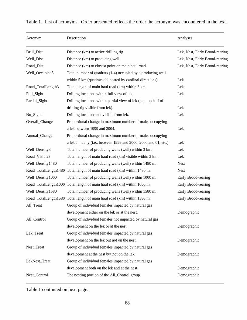
Table 1. List of acronyms. Order presented reflects the order the acronym was encountered in the text.

Acronym Description Analyses

Drill_Dist Distance (km) to active drilling rig. Lek, Nest, Early Brood-rearing

Well_Dist Distance (km) to producing well. Lek, Nest, Early Brood-rearing

Road_Dist Distance (km) to closest point on main haul road. Lek, Nest, Early Brood-rearing

Well_Occupied5 Total number of quadrats (1-4) occupied by a producing well

within 5 km (quadrats delineated by cardinal directions). Lek

Road_TotalLength3 Total length of main haul road (km) within 3 km. Lek

Full_Sight Drilling locations within full view of lek. Lek

Partial_Sight Drilling locations within partial view of lek (i.e., top half of

drilling rig visible from lek). Lek

No_Sight Drilling locations not visible from lek. Lek

Overall_Change Proportional change in maximum number of males occupying

a lek between 1999 and 2004. Lek

Annual_Change Proportional change in maximum number of males occupying

a lek annually (i.e., between 1999 and 2000, 2000 and 01, etc.). Lek

Well_Density3 Total number of producing wells (well) within 3 km. Lek

Road_Visible3 Total length of main haul road (km) visible within 3 km. Lek

Well_Density1480 Total number of producing wells (well) within 1480 m. Nest

Road_TotalLength1480 Total length of main haul road (km) within 1480 m. Nest

Well_Density1000 Total number of producing wells (well) within 1000 m. Early Brood-rearing

Road_TotalLength1000 Total length of main haul road (km) within 1000 m. Early Brood-rearing

Well_Density1580 Total number of producing wells (well) within 1580 m. Early Brood-rearing

Road_TotalLength1580 Total length of main haul road (km) within 1580 m. Early Brood-rearing

All_Treat Group of individual females impacted by natural gas

development either on the lek or at the nest . Demographic

All_Control Group of individual females not impacted by natural gas

development on the lek or at the nest. Demographic

Lek_Treat Group of individual females impacted by natural gas

development on the lek but not on the nest. Demographic

Nest_Treat Group of individual females impacted by natural gas

development at the nest but not on the lek. Demographic

LekNest_Treat Group of individual females impacted by natural gas

development both on the lek and at the nest. Demographic

Nest_Control The nesting portion of the All_Control group. Demographic

Table 1 continued on next page.

68

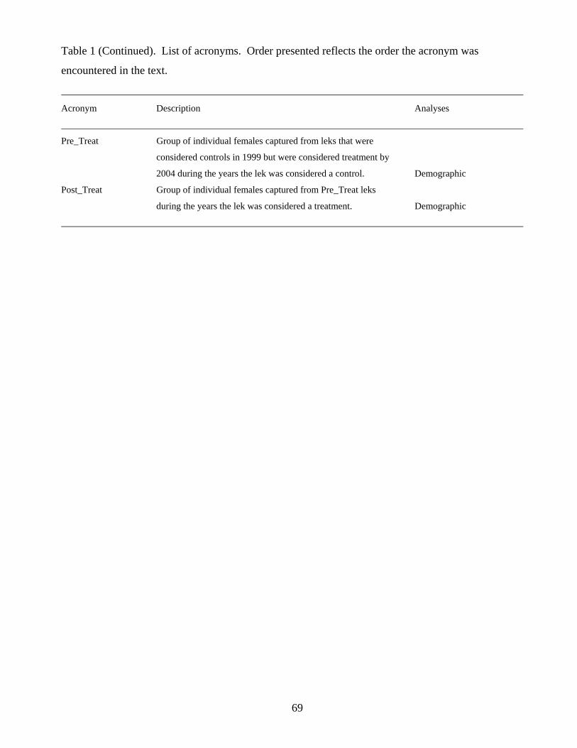
Table 1 (Continued). List of acronyms. Order presented reflects the order the acronym was

encountered in the text.

Acronym Description Analyses

Pre_Treat Group of individual females captured from leks that were

considered controls in 1999 but were considered treatment by

2004 during the years the lek was considered a control. Demographic

Post_Treat Group of individual females captured from Pre_Treat leks

during the years the lek was considered a treatment. Demographic

69

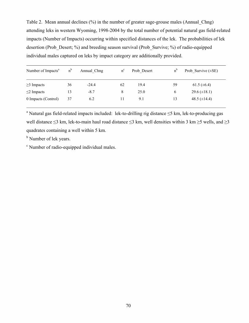
Table 2. Mean annual declines (%) in the number of greater sage-grouse males (Annual_Chng)

attending leks in western Wyoming, 1998-2004 by the total number of potential natural gas field-related

impacts (Number of Impacts) occurring within specified distances of the lek. The probabilities of lek

desertion (Prob_Desert; %) and breeding season survival (Prob_Survive; %) of radio-equipped

individual males captured on leks by impact category are additionally provided.

Number of Impactsa nb Annual_Chng nc Prob_Desert nb Prob_Survive (±SE)

≥3 Impacts 36 -24.4 62 19.4 59 61.5 (±6.4)

≤2 Impacts 13 -8.7 8 25.0 6 29.6 (±18.1)

0 Impacts (Control) 37 6.2 11 9.1 13 48.5 (±14.4)

a Natural gas field-related impacts included: lek-to-drilling rig distance ≤5 km, lek-to-producing gas

well distance ≤3 km, lek-to-main haul road distance ≤3 km, well densities within 3 km ≥5 wells, and ≥3

quadrates containing a well within 5 km. b Number of lek years. c Number of radio-equipped individual males.

70

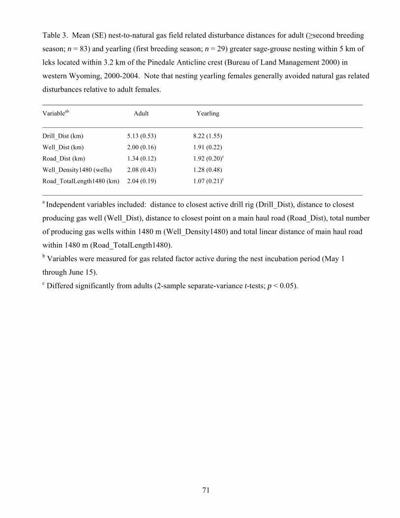
Table 3. Mean (SE) nest-to-natural gas field related disturbance distances for adult (≥second breeding

season; n = 83) and yearling (first breeding season; n = 29) greater sage-grouse nesting within 5 km of

leks located within 3.2 km of the Pinedale Anticline crest (Bureau of Land Management 2000) in

western Wyoming, 2000-2004. Note that nesting yearling females generally avoided natural gas related

disturbances relative to adult females.

Variableab Adult Yearling

Drill_Dist (km) 5.13 (0.53) 8.22 (1.55)

Well_Dist (km) 2.00 (0.16) 1.91 (0.22)

Road_Dist (km) 1.34 (0.12) 1.92 (0.20)c

Well_Density1480 (wells) 2.08 (0.43) 1.28 (0.48)

Road_TotalLength1480 (km) 2.04 (0.19) 1.07 (0.21)c

a Independent variables included: distance to closest active drill rig (Drill_Dist), distance to closest

producing gas well (Well_Dist), distance to closest point on a main haul road (Road_Dist), total number

of producing gas wells within 1480 m (Well_Density1480) and total linear distance of main haul road

within 1480 m (Road_TotalLength1480). b Variables were measured for gas related factor active during the nest incubation period (May 1

through June 15). c Differed significantly from adults (2-sample separate-variance t-tests; p < 0.05).

71

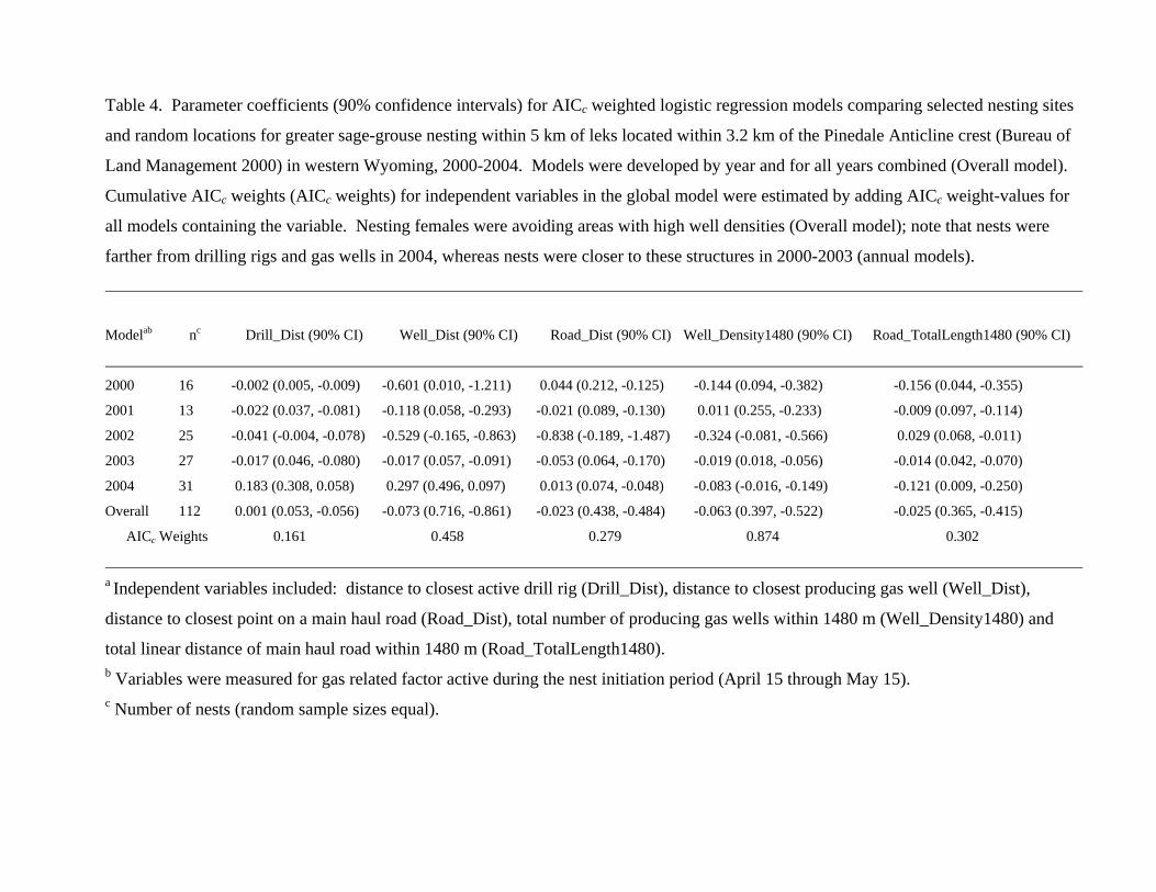
Table 4. Parameter coefficients (90% confidence intervals) for AICc weighted logistic regression models comparing selected nesting sites

and random locations for greater sage-grouse nesting within 5 km of leks located within 3.2 km of the Pinedale Anticline crest (Bureau of

Land Management 2000) in western Wyoming, 2000-2004. Models were developed by year and for all years combined (Overall model).

Cumulative AICc weights (AICc weights) for independent variables in the global model were estimated by adding AICc weight-values for

all models containing the variable. Nesting females were avoiding areas with high well densities (Overall model); note that nests were

farther from drilling rigs and gas wells in 2004, whereas nests were closer to these structures in 2000-2003 (annual models).

Modelab nc Drill_Dist (90% CI) Well_Dist (90% CI) Road_Dist (90% CI) Well_Density1480 (90% CI) Road_TotalLength1480 (90% CI)

2000 16 -0.002 (0.005, -0.009) -0.601 (0.010, -1.211) 0.044 (0.212, -0.125) -0.144 (0.094, -0.382) -0.156 (0.044, -0.355)

2001 13 -0.022 (0.037, -0.081) -0.118 (0.058, -0.293) -0.021 (0.089, -0.130) 0.011 (0.255, -0.233) -0.009 (0.097, -0.114)

2002 25 -0.041 (-0.004, -0.078) -0.529 (-0.165, -0.863) -0.838 (-0.189, -1.487) -0.324 (-0.081, -0.566) 0.029 (0.068, -0.011)

2003 27 -0.017 (0.046, -0.080) -0.017 (0.057, -0.091) -0.053 (0.064, -0.170) -0.019 (0.018, -0.056) -0.014 (0.042, -0.070)

2004 31 0.183 (0.308, 0.058) 0.297 (0.496, 0.097) 0.013 (0.074, -0.048) -0.083 (-0.016, -0.149) -0.121 (0.009, -0.250)

Overall 112 0.001 (0.053, -0.056) -0.073 (0.716, -0.861) -0.023 (0.438, -0.484) -0.063 (0.397, -0.522) -0.025 (0.365, -0.415)

AICc Weights 0.161 0.458 0.279 0.874 0.302

a Independent variables included: distance to closest active drill rig (Drill_Dist), distance to closest producing gas well (Well_Dist),

distance to closest point on a main haul road (Road_Dist), total number of producing gas wells within 1480 m (Well_Density1480) and

total linear distance of main haul road within 1480 m (Road_TotalLength1480). b Variables were measured for gas related factor active during the nest initiation period (April 15 through May 15). c Number of nests (random sample sizes equal).

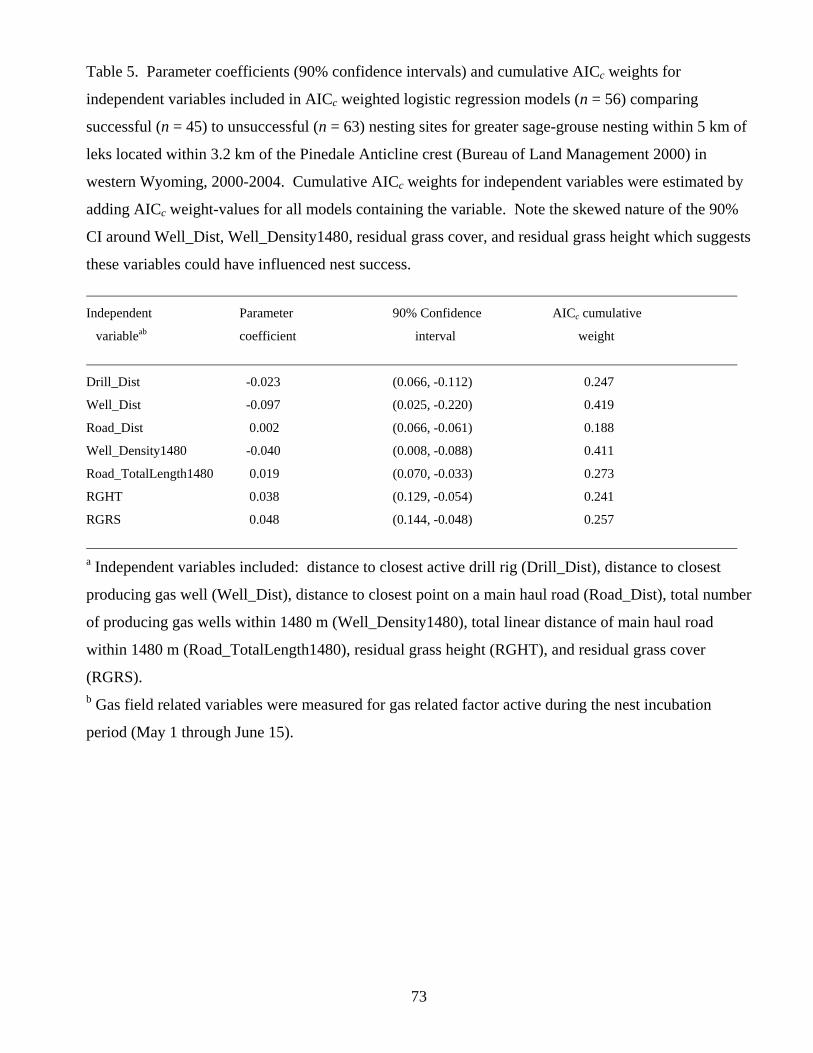
Table 5. Parameter coefficients (90% confidence intervals) and cumulative AICc weights for

independent variables included in AICc weighted logistic regression models (n = 56) comparing

successful (n = 45) to unsuccessful (n = 63) nesting sites for greater sage-grouse nesting within 5 km of

leks located within 3.2 km of the Pinedale Anticline crest (Bureau of Land Management 2000) in

western Wyoming, 2000-2004. Cumulative AICc weights for independent variables were estimated by

adding AICc weight-values for all models containing the variable. Note the skewed nature of the 90%

CI around Well_Dist, Well_Density1480, residual grass cover, and residual grass height which suggests

these variables could have influenced nest success.

Independent Parameter 90% Confidence AICc cumulative

variableab coefficient interval weight

Drill_Dist -0.023 (0.066, -0.112) 0.247

Well_Dist -0.097 (0.025, -0.220) 0.419

Road_Dist 0.002 (0.066, -0.061) 0.188

Well_Density1480 -0.040 (0.008, -0.088) 0.411

Road_TotalLength1480 0.019 (0.070, -0.033) 0.273

RGHT 0.038 (0.129, -0.054) 0.241

RGRS 0.048 (0.144, -0.048) 0.257



of producing gas wells within 1480 m (Well_Density1480), total linear distance of main haul road

within 1480 m (Road_TotalLength1480), residual grass height (RGHT), and residual grass cover

(RGRS). b Gas field related variables were measured for gas related factor active during the nest incubation

period (May 1 through June 15).

73

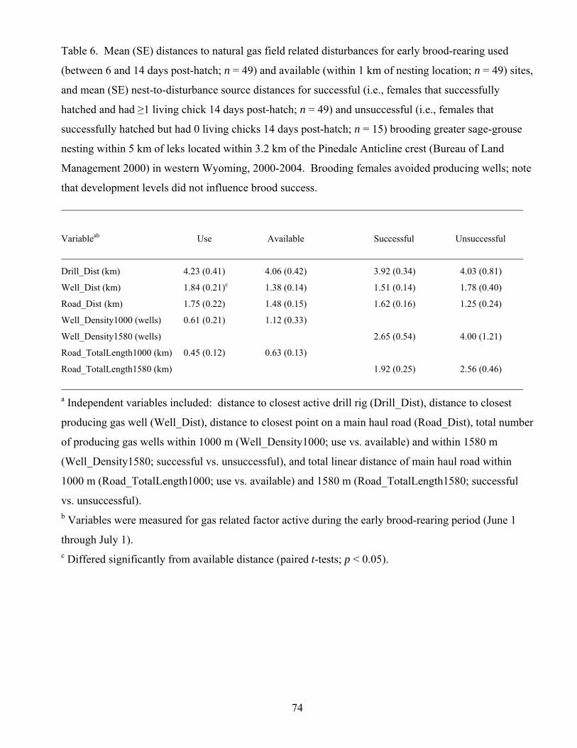
Table 6. Mean (SE) distances to natural gas field related disturbances for early brood-rearing used

(between 6 and 14 days post-hatch; n = 49) and available (within 1 km of nesting location; n = 49) sites,

and mean (SE) nest-to-disturbance source distances for successful (i.e., females that successfully

hatched and had ≥1 living chick 14 days post-hatch; n = 49) and unsuccessful (i.e., females that

successfully hatched but had 0 living chicks 14 days post-hatch; n = 15) brooding greater sage-grouse

nesting within 5 km of leks located within 3.2 km of the Pinedale Anticline crest (Bureau of Land

Management 2000) in western Wyoming, 2000-2004. Brooding females avoided producing wells; note

that development levels did not influence brood success.

Variableab Use Available Successful Unsuccessful

Drill_Dist (km) 4.23 (0.41) 4.06 (0.42) 3.92 (0.34) 4.03 (0.81)

Well_Dist (km) 1.84 (0.21)c 1.38 (0.14) 1.51 (0.14) 1.78 (0.40)

Road_Dist (km) 1.75 (0.22) 1.48 (0.15) 1.62 (0.16) 1.25 (0.24)



Road_TotalLength1000 (km) 0.45 (0.12) 0.63 (0.13)

Road_TotalLength1580 (km) 1.92 (0.25) 2.56 (0.46)



of producing gas wells within 1000 m (Well_Density1000; use vs. available) and within 1580 m

(Well_Density1580; successful vs. unsuccessful), and total linear distance of main haul road within

1000 m (Road_TotalLength1000; use vs. available) and 1580 m (Road_TotalLength1580; successful

vs. unsuccessful). b Variables were measured for gas related factor active during the early brood-rearing period (June 1

through July 1). c Differed significantly from available distance (paired t-tests; p < 0.05).

74

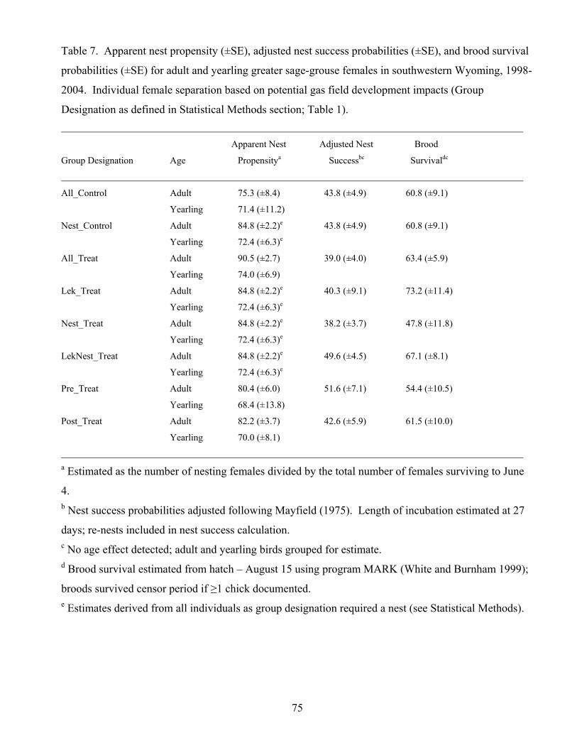
Table 7. Apparent nest propensity (±SE), adjusted nest success probabilities (±SE), and brood survival

probabilities (±SE) for adult and yearling greater sage-grouse females in southwestern Wyoming, 1998-

2004. Individual female separation based on potential gas field development impacts (Group

Designation as defined in Statistical Methods section; Table 1).

Apparent Nest Adjusted Nest Brood

Group Designation Age Propensitya Successbc Survivaldc

All_Control Adult 75.3 (±8.4) 43.8 (±4.9) 60.8 (±9.1)

Yearling 71.4 (±11.2)

Nest_Control Adult 84.8 (±2.2)e 43.8 (±4.9) 60.8 (±9.1)

Yearling 72.4 (±6.3)e

All_Treat Adult 90.5 (±2.7) 39.0 (±4.0) 63.4 (±5.9)

Yearling 74.0 (±6.9)

Lek_Treat Adult 84.8 (±2.2)e 40.3 (±9.1) 73.2 (±11.4)


Nest_Treat Adult 84.8 (±2.2)e 38.2 (±3.7) 47.8 (±11.8)


LekNest_Treat Adult 84.8 (±2.2)e 49.6 (±4.5) 67.1 (±8.1)


Pre_Treat Adult 80.4 (±6.0) 51.6 (±7.1) 54.4 (±10.5)

Yearling 68.4 (±13.8)

Post_Treat Adult 82.2 (±3.7) 42.6 (±5.9) 61.5 (±10.0)

Yearling 70.0 (±8.1)

a Estimated as the number of nesting females divided by the total number of females surviving to June

4. b Nest success probabilities adjusted following Mayfield (1975). Length of incubation estimated at 27

days; re-nests included in nest success calculation. c No age effect detected; adult and yearling birds grouped for estimate. d Brood survival estimated from hatch – August 15 using program MARK (White and Burnham 1999);

broods survived censor period if ≥1 chick documented. e Estimates derived from all individuals as group designation required a nest (see Statistical Methods).

75

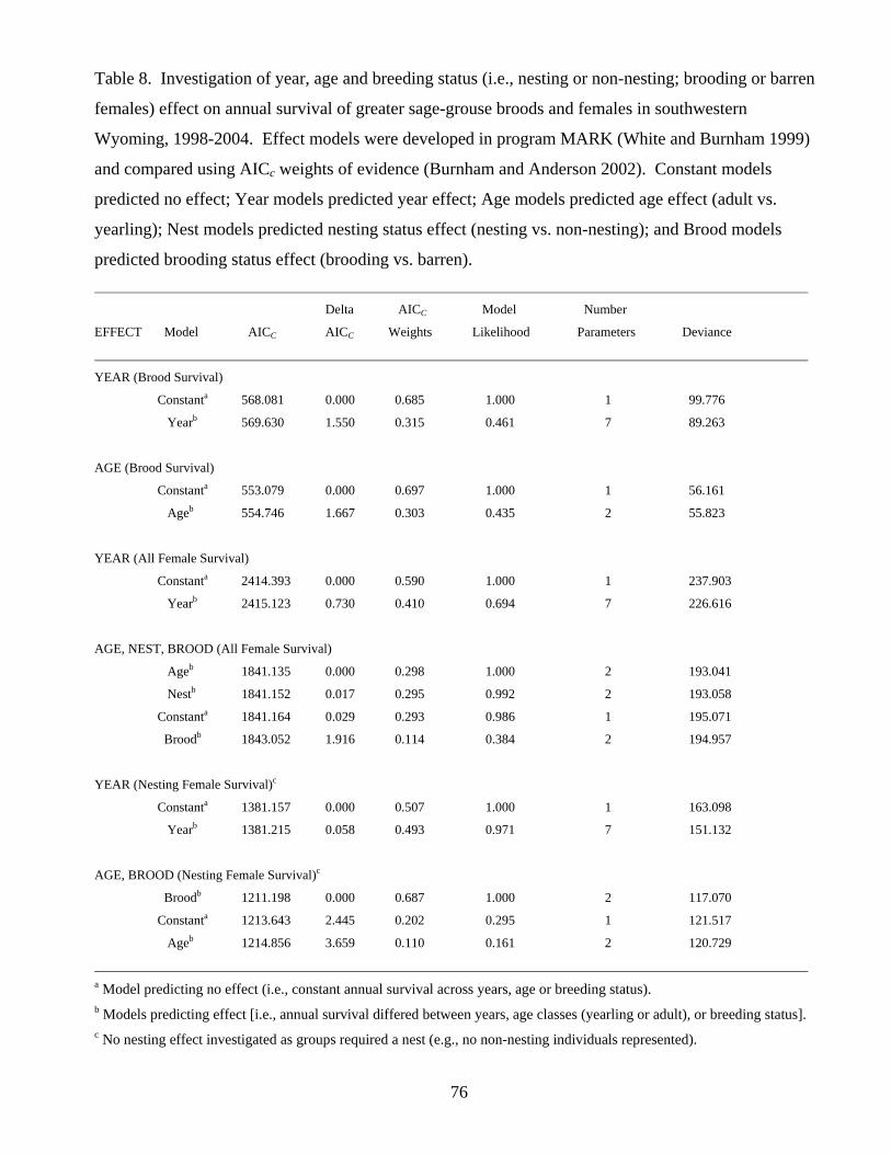
Table 8. Investigation of year, age and breeding status (i.e., nesting or non-nesting; brooding or barren

females) effect on annual survival of greater sage-grouse broods and females in southwestern

Wyoming, 1998-2004. Effect models were developed in program MARK (White and Burnham 1999)

and compared using AICc weights of evidence (Burnham and Anderson 2002). Constant models

predicted no effect; Year models predicted year effect; Age models predicted age effect (adult vs.

yearling); Nest models predicted nesting status effect (nesting vs. non-nesting); and Brood models

predicted brooding status effect (brooding vs. barren).

Delta AICC Model Number

EFFECT Model AICC AICC Weights Likelihood Parameters Deviance

YEAR (Brood Survival)

Constanta 568.081 0.000 0.685 1.000 1 99.776

Yearb 569.630 1.550 0.315 0.461 7 89.263

AGE (Brood Survival)

Constanta 553.079 0.000 0.697 1.000 1 56.161

Ageb 554.746 1.667 0.303 0.435 2 55.823

YEAR (All Female Survival)

Constanta 2414.393 0.000 0.590 1.000 1 237.903

Yearb 2415.123 0.730 0.410 0.694 7 226.616

AGE, NEST, BROOD (All Female Survival)

Ageb 1841.135 0.000 0.298 1.000 2 193.041

Nestb 1841.152 0.017 0.295 0.992 2 193.058

Constanta 1841.164 0.029 0.293 0.986 1 195.071

Broodb 1843.052 1.916 0.114 0.384 2 194.957

YEAR (Nesting Female Survival)c

Constanta 1381.157 0.000 0.507 1.000 1 163.098

Yearb 1381.215 0.058 0.493 0.971 7 151.132

AGE, BROOD (Nesting Female Survival)c

Broodb 1211.198 0.000 0.687 1.000 2 117.070

Constanta 1213.643 2.445 0.202 0.295 1 121.517

Ageb 1214.856 3.659 0.110 0.161 2 120.729

a Model predicting no effect (i.e., constant annual survival across years, age or breeding status). b Models predicting effect [i.e., annual survival differed between years, age classes (yearling or adult), or breeding status]. c No nesting effect investigated as groups required a nest (e.g., no non-nesting individuals represented).

76

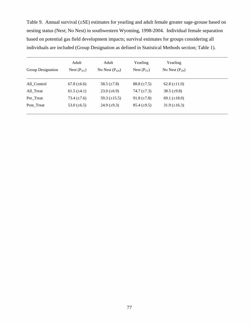
Table 9. Annual survival (±SE) estimates for yearling and adult female greater sage-grouse based on

nesting status (Nest; No Nest) in southwestern Wyoming, 1998-2004. Individual female separation

based on potential gas field development impacts; survival estimates for groups considering all

individuals are included (Group Designation as defined in Statistical Methods section; Table 1).

Adult Adult Yearling Yearling

Group Designation Nest (PAY) No Nest (PAN) Nest (P2Y) No Nest (P2N)

All_Control 67.8 (±6.6) 58.5 (±7.8) 88.8 (±7.5) 62.8 (±11.0)

All_Treat 61.5 (±4.1) 23.0 (±6.9) 74.7 (±7.3) 38.5 (±9.8)

Pre_Treat 73.4 (±7.6) 59.3 (±15.5) 91.8 (±7.8) 69.1 (±18.0)

Post_Treat 53.0 (±6.5) 24.9 (±9.3) 85.4 (±9.5) 31.9 (±16.3)

77

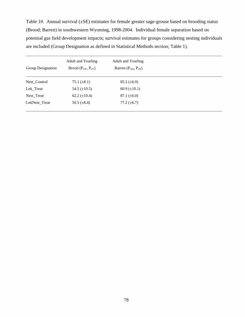
Table 10. Annual survival (±SE) estimates for female greater sage-grouse based on brooding status

(Brood; Barren) in southwestern Wyoming, 1998-2004. Individual female separation based on

potential gas field development impacts; survival estimates for groups considering nesting individuals

are included (Group Designation as defined in Statistical Methods section; Table 1).

Adult and Yearling Adult and Yearling

Group Designation Brood (PAY, P2Y) Barren (PAN, P2N)

Nest_Control 75.1 (±8.1) 85.5 (±6.0)

Lek_Treat 54.5 (±10.5) 60.9 (±10.1)

Nest_Treat 62.2 (±10.4) 87.1 (±6.0)

LekNest_Treat 50.5 (±8.4) 77.2 (±6.7)

78

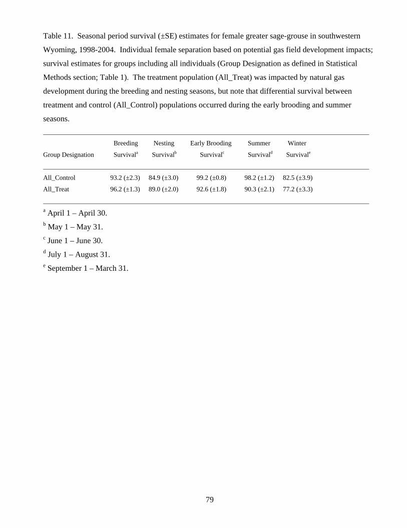
Table 11. Seasonal period survival (±SE) estimates for female greater sage-grouse in southwestern

Wyoming, 1998-2004. Individual female separation based on potential gas field development impacts;

survival estimates for groups including all individuals (Group Designation as defined in Statistical

Methods section; Table 1). The treatment population (All_Treat) was impacted by natural gas

development during the breeding and nesting seasons, but note that differential survival between

treatment and control (All_Control) populations occurred during the early brooding and summer

seasons.

Breeding Nesting Early Brooding Summer Winter

Group Designation Survivala Survivalb Survivalc Survivald Survivale

All_Control 93.2 (±2.3) 84.9 (±3.0) 99.2 (±0.8) 98.2 (±1.2) 82.5 (±3.9)

All_Treat 96.2 (±1.3) 89.0 (±2.0) 92.6 (±1.8) 90.3 (±2.1) 77.2 (±3.3)

a April 1 – April 30. b May 1 – May 31. c June 1 – June 30. d July 1 – August 31. e September 1 – March 31.

79

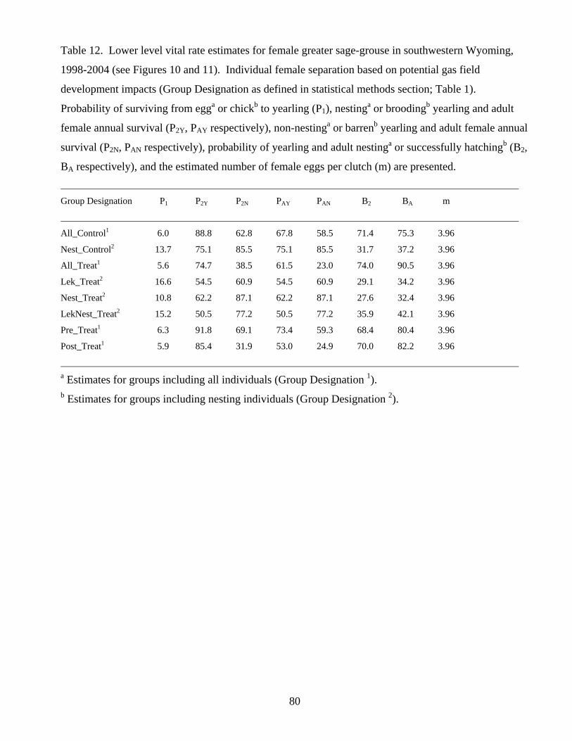
Table 12. Lower level vital rate estimates for female greater sage-grouse in southwestern Wyoming,

1998-2004 (see Figures 10 and 11). Individual female separation based on potential gas field

development impacts (Group Designation as defined in statistical methods section; Table 1).

Probability of surviving from egga or chickb to yearling (P1), nestinga or broodingb yearling and adult

female annual survival (P2Y, PAY respectively), non-nestinga or barrenb yearling and adult female annual

survival (P2N, PAN respectively), probability of yearling and adult nestinga or successfully hatchingb (B2,

BBA respectively), and the estimated number of female eggs per clutch (m) are presented.

Group Designation P1 P2Y P2N

PAY PAN B2

BA m

All_Control1 6.0 88.8 62.8 67.8 58.5 71.4 75.3 3.96

Nest_Control2 13.7 75.1 85.5 75.1 85.5 31.7 37.2 3.96

All_Treat1 5.6 74.7 38.5 61.5 23.0 74.0 90.5 3.96

Lek_Treat2 16.6 54.5 60.9 54.5 60.9 29.1 34.2 3.96

Nest_Treat2 10.8 62.2 87.1 62.2 87.1 27.6 32.4 3.96

LekNest_Treat2 15.2 50.5 77.2 50.5 77.2 35.9 42.1 3.96

Pre_Treat1 6.3 91.8 69.1 73.4 59.3 68.4 80.4 3.96

Post_Treat1 5.9 85.4 31.9 53.0 24.9 70.0 82.2 3.96

a Estimates for groups including all individuals (Group Designation 1). b Estimates for groups including nesting individuals (Group Designation 2).

80

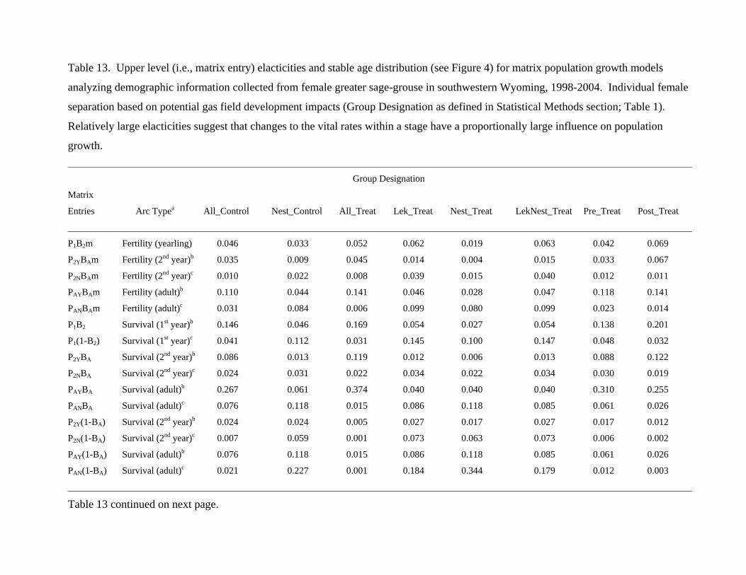
Table 13. Upper level (i.e., matrix entry) elacticities and stable age distribution (see Figure 4) for matrix population growth models

analyzing demographic information collected from female greater sage-grouse in southwestern Wyoming, 1998-2004. Individual female

separation based on potential gas field development impacts (Group Designation as defined in Statistical Methods section; Table 1).

Relatively large elacticities suggest that changes to the vital rates within a stage have a proportionally large influence on population

growth.

Group Designation

Matrix

Entries Arc Typea All_Control Nest_Control All_Treat Lek_Treat Nest_Treat LekNest_Treat Pre_Treat Post_Treat

P1B2m Fertility (yearling) 0.046 0.033 0.052 0.062 0.019 0.063 0.042 0.069

P2YBAm Fertility (2nd year)b 0.035 0.009 0.045 0.014 0.004 0.015 0.033 0.067

P2NBAm Fertility (2nd year)c 0.010 0.022 0.008 0.039 0.015 0.040 0.012 0.011

PAYBAm Fertility (adult)b 0.110 0.044 0.141 0.046 0.028 0.047 0.118 0.141

PANBAm Fertility (adult)c 0.031 0.084 0.006 0.099 0.080 0.099 0.023 0.014

P1B2 Survival (1st year)b 0.146 0.046 0.169 0.054 0.027 0.054 0.138 0.201

P1(1-B2) Survival (1st year)c 0.041 0.112 0.031 0.145 0.100 0.147 0.048 0.032

P2YBA Survival (2nd year)b 0.086 0.013 0.119 0.012 0.006 0.013 0.088 0.122

P2NBA Survival (2nd year)c 0.024 0.031 0.022 0.034 0.022 0.034 0.030 0.019

PAYBA Survival (adult)b 0.267 0.061 0.374 0.040 0.040 0.040 0.310 0.255

PANBA Survival (adult)c 0.076 0.118 0.015 0.086 0.118 0.085 0.061 0.026

P2Y(1-BA) Survival (2nd year)b 0.024 0.024 0.005 0.027 0.017 0.027 0.017 0.012

P2N(1-BA) Survival (2nd year)c 0.007 0.059 0.001 0.073 0.063 0.073 0.006 0.002

PAY(1-BA) Survival (adult)b 0.076 0.118 0.015 0.086 0.118 0.085 0.061 0.026

PAN(1-BA) Survival (adult)c 0.021 0.227 0.001 0.184 0.344 0.179 0.012 0.003

Table 13 continued on next page.

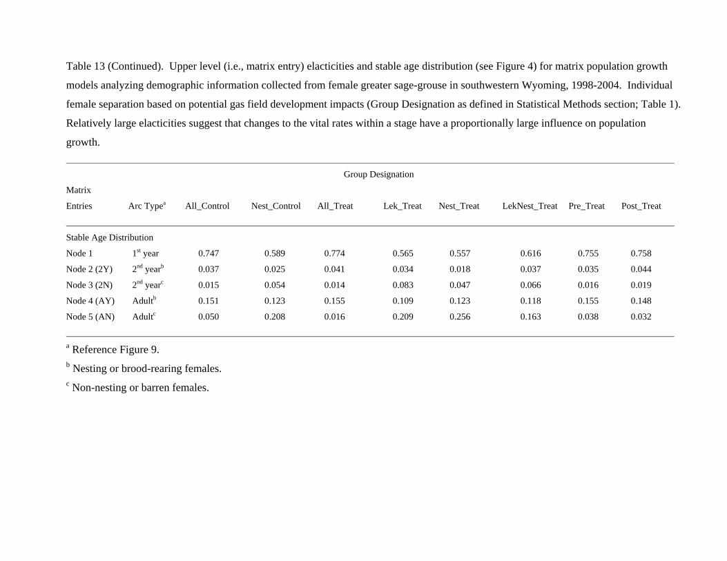
Table 13 (Continued). Upper level (i.e., matrix entry) elacticities and stable age distribution (see Figure 4) for matrix population growth

models analyzing demographic information collected from female greater sage-grouse in southwestern Wyoming, 1998-2004. Individual

female separation based on potential gas field development impacts (Group Designation as defined in Statistical Methods section; Table 1).

Relatively large elacticities suggest that changes to the vital rates within a stage have a proportionally large influence on population

growth.

Group Designation

Matrix

Entries Arc Typea All_Control Nest_Control All_Treat Lek_Treat Nest_Treat LekNest_Treat Pre_Treat Post_Treat

Stable Age Distribution

Node 1 1st year 0.747 0.589 0.774 0.565 0.557 0.616 0.755 0.758

Node 2 (2Y) 2nd yearb 0.037 0.025 0.041 0.034 0.018 0.037 0.035 0.044

Node 3 (2N) 2nd yearc 0.015 0.054 0.014 0.083 0.047 0.066 0.016 0.019

Node 4 (AY) Adultb 0.151 0.123 0.155 0.109 0.123 0.118 0.155 0.148

Node 5 (AN) Adultc 0.050 0.208 0.016 0.209 0.256 0.163 0.038 0.032

a Reference Figure 9. b Nesting or brood-rearing females. c Non-nesting or barren females.

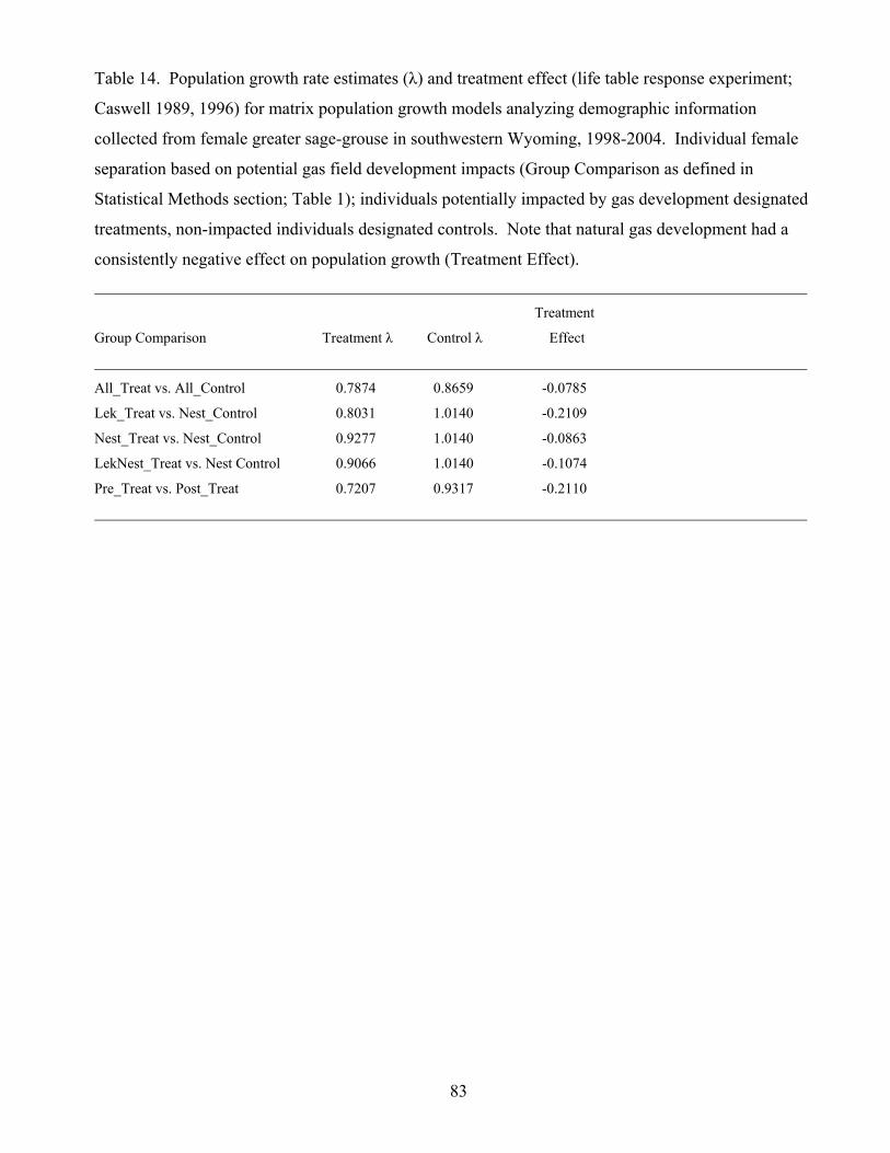
Table 14. Population growth rate estimates (λ) and treatment effect (life table response experiment;

Caswell 1989, 1996) for matrix population growth models analyzing demographic information

collected from female greater sage-grouse in southwestern Wyoming, 1998-2004. Individual female

separation based on potential gas field development impacts (Group Comparison as defined in

Statistical Methods section; Table 1); individuals potentially impacted by gas development designated

treatments, non-impacted individuals designated controls. Note that natural gas development had a

consistently negative effect on population growth (Treatment Effect).

Treatment

Group Comparison Treatment λ Control λ Effect

All_Treat vs. All_Control 0.7874 0.8659 -0.0785

Lek_Treat vs. Nest_Control 0.8031 1.0140 -0.2109

Nest_Treat vs. Nest_Control 0.9277 1.0140 -0.0863

LekNest_Treat vs. Nest Control 0.9066 1.0140 -0.1074

Pre_Treat vs. Post_Treat 0.7207 0.9317 -0.2110

83

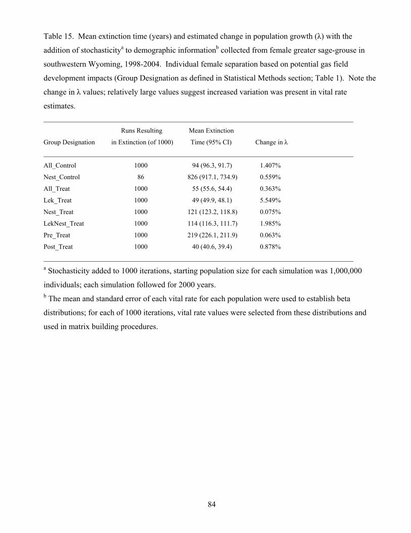
Table 15. Mean extinction time (years) and estimated change in population growth (λ) with the

addition of stochasticitya to demographic informationb collected from female greater sage-grouse in

southwestern Wyoming, 1998-2004. Individual female separation based on potential gas field

development impacts (Group Designation as defined in Statistical Methods section; Table 1). Note the

change in λ values; relatively large values suggest increased variation was present in vital rate

estimates.

Runs Resulting Mean Extinction

Group Designation in Extinction (of 1000) Time (95% CI) Change in λ

All_Control 1000 94 (96.3, 91.7) 1.407%

Nest_Control 86 826 (917.1, 734.9) 0.559%

All_Treat 1000 55 (55.6, 54.4) 0.363%

Lek_Treat 1000 49 (49.9, 48.1) 5.549%

Nest_Treat 1000 121 (123.2, 118.8) 0.075%

LekNest_Treat 1000 114 (116.3, 111.7) 1.985%

Pre_Treat 1000 219 (226.1, 211.9) 0.063%

Post_Treat 1000 40 (40.6, 39.4) 0.878%

a Stochasticity added to 1000 iterations, starting population size for each simulation was 1,000,000

individuals; each simulation followed for 2000 years. b The mean and standard error of each vital rate for each population were used to establish beta

distributions; for each of 1000 iterations, vital rate values were selected from these distributions and

used in matrix building procedures.

84

Figure 1. Greater sage-grouse study location in southwestern Wyoming, 1998-2004. General outlines

of the Pinedale Anticline Project Area (PAPA) and the Jonah II natural gas field (gas field boundaries

adapted from Bureau of Land Management 2000), and general study lek (n = 21) locations are provided

for reference.

85

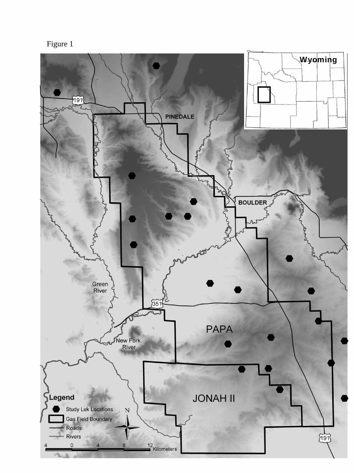
Figure 1

Wyoming

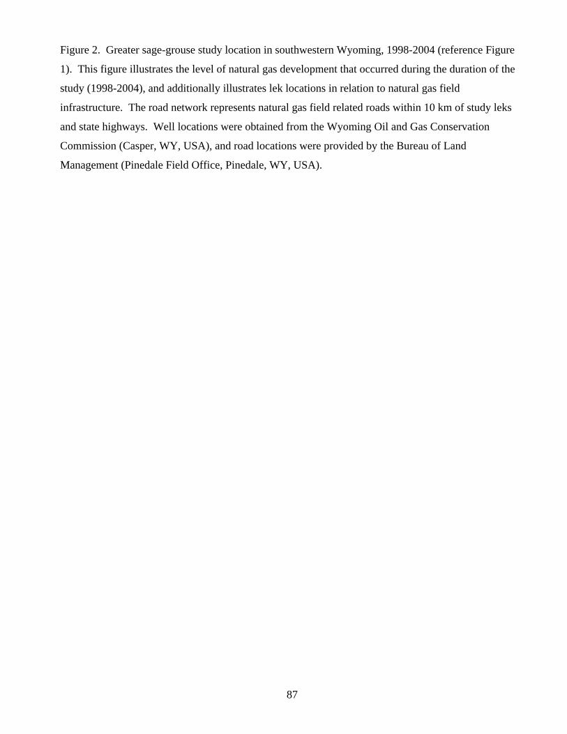
Figure 2. Greater sage-grouse study location in southwestern Wyoming, 1998-2004 (reference Figure

1). This figure illustrates the level of natural gas development that occurred during the duration of the

study (1998-2004), and additionally illustrates lek locations in relation to natural gas field

infrastructure. The road network represents natural gas field related roads within 10 km of study leks

and state highways. Well locations were obtained from the Wyoming Oil and Gas Conservation

Commission (Casper, WY, USA), and road locations were provided by the Bureau of Land

Management (Pinedale Field Office, Pinedale, WY, USA).

87

Figure 2

Figure 3. Greater sage-grouse study location in southwestern Wyoming, 1998-2004 (reference Figure

1). The dashed lines are 5 km buffers around known leks located within 3.2 km of the Pinedale

Anticline crest, and represent the spatial area used for nesting and early brood-rearing habitat selection.

This figure illustrates the level of natural gas development that occurred during the female habitat

selection portion of the study (2000-2004). The road network represents natural gas field related roads

within 10 km of study leks and state highways. Well locations were obtained from the Wyoming Oil

and Gas Conservation Commission (Casper, WY, USA), and road locations were provided by the

Bureau of Land Management (Pinedale Field Office, Pinedale, WY, USA).

89

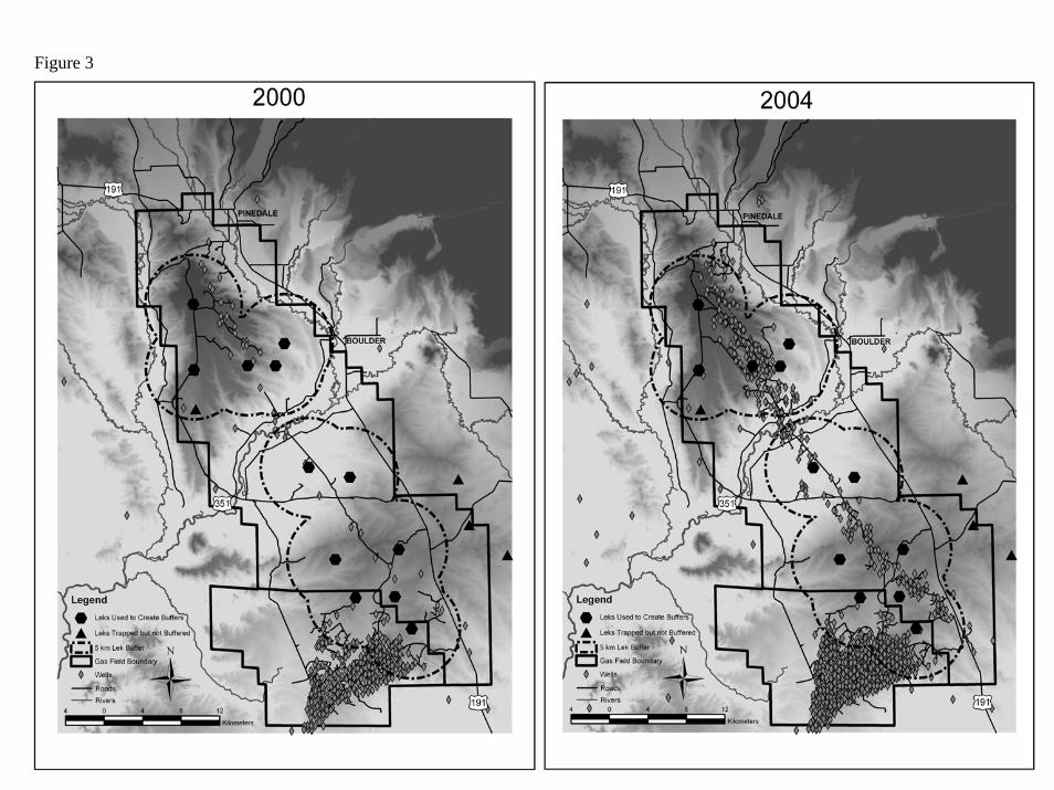
Figure 3

Figure 4. Regression relationship between overall change (%) in the number of greater sage-grouse

males attending leks in southwestern Wyoming, 1998-2004 and principal component 1 scores.

Principal component 1 included: average annual distance (km) from leks to closest drilling rig active

during the breeding season, distance (km) to closest producing gas well, and distance (km) to closest

point on a main haul road; the total number of quadrats (categorized by the cardinal directions)

occupied by a producing well within 5 km of leks; and the total length (km) of main haul road within 3

km of leks. Note that the relationship suggests that as natural gas development levels increase

relatively near a greater sage-grouse lek, male lek attendance approaches 100% decline (i.e., lek

inactivity; notice Y-axis scale).

91

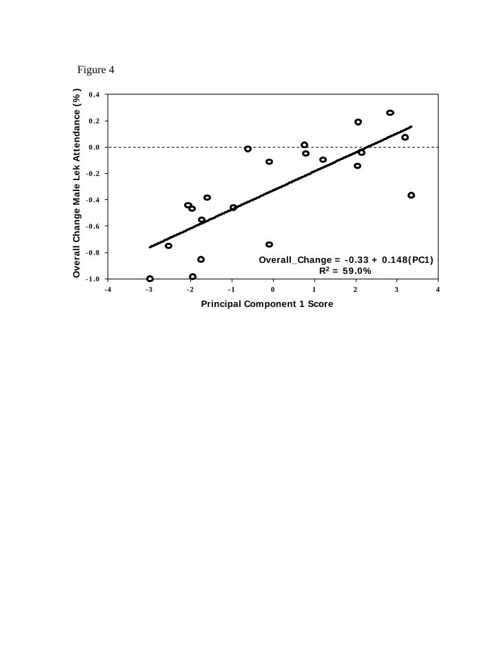
-4 -3 -2 -1 0 1 2 3 4-1 .0

-0 .8

-0 .6

-0 .4

-0 .2

0 .0

0 .2

0 .4

Principal Component 1 Score

Ove

rall

Ch

ange

Mal

e Le

k A

tten

dan

ce (

%)

Overall_Change = -0.33 + 0.148(PC1)R2 = 59.0%

Figure 4

Figure 5. Regression relationships between overall change (%) in the number of greater sage-grouse

males attending leks in southwestern Wyoming, 1998-2004 and average annual distance from leks to

closest drilling rig active during the breeding season, closest producing natural gas well, and closest

point on a main haul road. Notice scale differences on X-axes. Note that the curvilinear relationships

suggest a distance-effect to greater sage-grouse male lek attendance relative to natural gas field-related

structures.

93

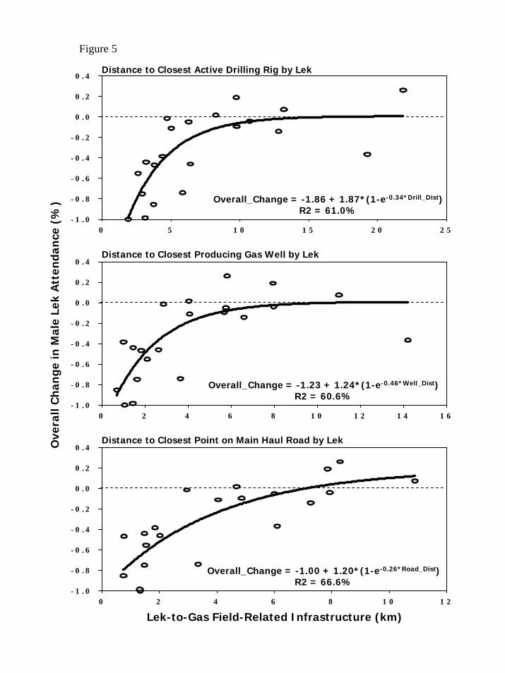
0 2 4 6 8 1 0 1 2- 1 . 0

- 0 . 8

- 0 . 6

- 0 . 4

- 0 . 2

0 . 0

0 . 2

0 . 4

0 2 4 6 8 1 0 1 2 1 4 1 6- 1 . 0

- 0 . 8

- 0 . 6

- 0 . 4

- 0 . 2

0 . 0

0 . 2

0 . 4

0 5 1 0 1 5 2 0 2 5- 1 . 0

- 0 . 8

- 0 . 6

- 0 . 4

- 0 . 2

0 . 0

0 . 2

0 . 4

Ove

rall

Ch

ange

in M

ale

Lek

Att

enda

nce

(%

)

Lek-to-Gas Field-Related Infrastructure (km)

Overall_Change = -1.86 + 1.87*(1-e-0.34*Drill_Dist)R2 = 61.0%

Distance to Closest Producing Gas Well by Lek

Distance to Closest Point on Main Haul Road by Lek

Overall_Change = -1.23 + 1.24*(1-e-0.46*Well_Dist)R2 = 60.6%

Overall_Change = -1.00 + 1.20*(1-e-0.26*Road_Dist)R2 = 66.6%

Distance to Closest Active Drilling Rig by Lek

Figure 5

Figure 6. Mean annual change (%) in the number of greater sage-grouse males attending leks in

southwestern Wyoming, 1998-2004 by lek-to-closest drilling rig active during the breeding season

distance categories, lek-to-closest producing natural gas well distance categories, and lek-to-closest

point on a main haul road distance categories. Solid bars differed significantly from controls (separate

variance, 2-sample t-tests; p ≤ 0.05). Error bars represent 95% confidence intervals. Control distances

were determined from curvilinear regression relationships (Figure 3) using geostatistical methods

(Royle et al. 1980). Note that drilling rigs within 5 km, producing wells within 3 km, and main haul

roads within 3 km of a lek negatively influenced greater sage-grouse male lek attendance.

95

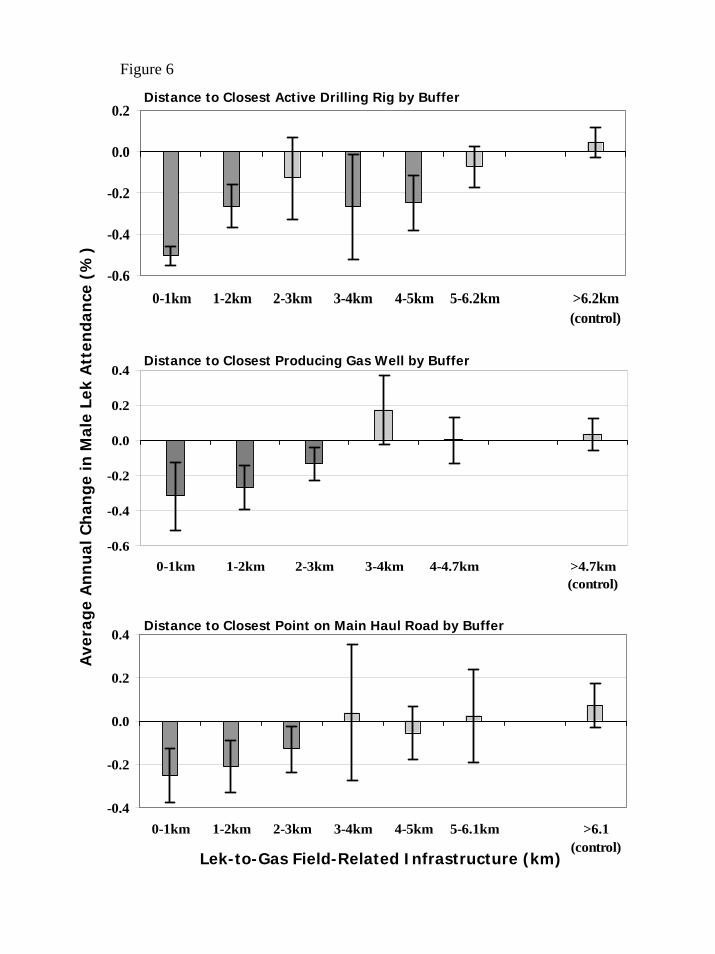
-0.4

-0.2

0.0

0.2

0.4

0-1km 1-2km 2-3km 3-4km 4-5km 5-6.1km >6.1(control)

-0.6

-0.4

-0.2

0.0

0.2

0.4

0-1km 1-2km 2-3km 3-4km 4-4.7km >4.7km(control)

-0.6

-0.4

0-1km 1-2km 2-3km 3-4km 4-5km 5-6.2km >6.2km(control)

Ave

rage

An

nu

al C

han

ge in

Mal

e Le

k A

tten

dan

ce (

%)

Lek-to-Gas Field-Related Infrastructure (km)

Distance to Closest Producing Gas Well by Buffer

Distance to Closest Point on Main Haul Road by Buffer

-0.2

0.0

0.2Distance to Closest Active Drilling Rig by Buffer

Figure 6

Figure 7. Nest probabilities relative to natural gas development levels generated from an AICc

weighted logistic regression model comparing selected nesting sites (n = 112) and random locations (n

= 112) for greater sage-grouse nesting within 5 km of leks located within 3.2 km of the Pinedale

Anticline crest (Bureau of Land Management 2000) in southwestern Wyoming, 2000-2004.

Independent variables included: distance to closest active drill rig (Drill_Dist), distance to closest


of producing gas wells within 1480m (Total_Well1480) and total linear distance of main haul road

within 1480m (Total_Road1480). Variables were measured for gas related factor active during the nest

initiation period (Apr 15 through May 15). Average AICc weighted logistic regression model used to

estimate probabilities: Nest probability = e^[0.364 – 0.001(Drill_Dist) – 0.073(Well_Dist) –

0.023(Road_Dist) – 0.063(Total_Well1480) – 0.025(Total_Road1480)]. Levels of gas field

development (X-axis) represent the range of values witnessed for nesting females, and ranged between:

0.7 – 38.0 km for Drill_Dist, 0.1 – 9.2 km for Well_Dist, 0.01 – 6.2 for Road_Dist, 0 – 21 wells for

Total_Well1480, and 0 – 7.1 km for Total_Road1480.

97

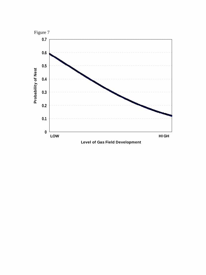
0

0.1

0.2

0.3

0.4

0.5

0.6

0.7

Level of Gas Field Development LOW HIGH

Pro

babi

lity

of N

est

Figure 7

Figure 8. Annual sample size and percent normal precipitation for female greater sage-grouse in

southwestern Wyoming, 1998-2004. Pre_Treat and Post_Treat groups (defined in Statistical Methods

section) compared. Note sample sizes in 2001 and 2002, suggesting that population growth differences

pre- versus post-treatment were not unduly confounded by drought conditions.

99

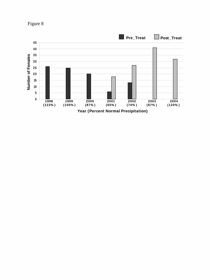
0

5

10

15

2 0

2 5

3 0

3 5

4 0

4 5

Num

ber o

f Fem

ales

Figure 8

Pre_Treat Post_Treat

1998 1999 2000 2001 2002 2003 2004 (123%) (100%) (87%) (65%) (74%) (87%) (120%)

Year (Percent Normal Precipitation)

Figure 9. Life-cycle diagram and matrix for a 5 stage population growth model of female greater sage-

grouse in southwestern Wyoming, 1998-2004. Notations for matrix entries defined in Statistical

Methods section and Table 12. Separation into stages based on differential survival estimated using

program MARK (White and Burnham 1999; Table 8).

101

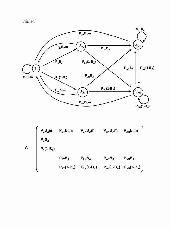
22Y

1

5AN32N

4AY

PAYBAm

P2NBAm

P2YBAm

PANBAm

P2Y(1-BA)

P2NBA

P1B2

P1(1-B2)

PANBA

P2YBA

P2N(1-BA)

PAY(1-BA)

P1B2m

PAYBA

PAN(1-BA)

A =

P1B2m P2YBAm P2NBAm PAYBAm PANBAm

P1B2

P1(1-B2)

P2YBA P2NBA PAYBA PANBA

P2Y(1-BA) P2N(1-BA) PAY(1-BA) PAN(1-BA)

Figure 9

Figure 10. Life table response experiment (Caswell 1989, 1996) results from population growth models

analyzing demographic information collected from female greater sage-grouse in southwestern

Wyoming, 1998-2004. Bars indicate the contribution of vital rates to the difference in population

growth between treatment and control populations. Vital rates include: yearling and adult nesting

propensity [NP(y) and NP(a) respectively], the number of female eggs per clutch (#Eggs), nest success

probability (NS), brood survival probability (BS), Chick summer (CS) and winter (CW) survival,

nesting yearling and adult female annual survival [P2y and Pay respectively], and non-nesting yearling

and adult annual survival [P2n and Pan respectively]. Groups considering all individuals (as defined in

Statistical Methods section) are presented. Note that lower annual survival of nesting and non-nesting

adult treatment females was primarily responsible for differences in population growth (Table 14).

103

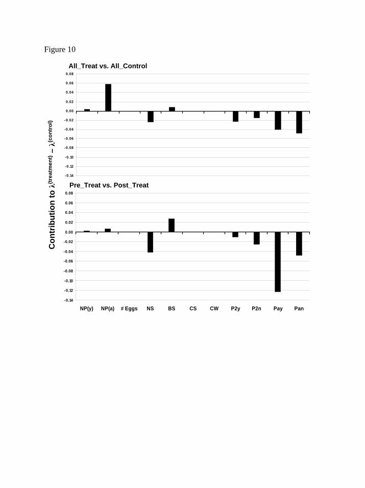
All_Treat vs. All_Control

Pre_Treat vs. Post_Treat

Con

trib

utio

n to

λ(tr

eatm

ent)

–λ(

cont

rol)

Figure 10

-0.14

-0.12

-0.10

-0.08

-0.06

-0.04

-0.02

0.00

0.02

0.04

0.06

0.08

NP(y) NP(a) # Eggs NS BS CS CW P2y P2n Pay Pan

-0.14

-0.12

-0.10

-0.08

-0.06

-0.04

-0.02

0.00

0.02

0.04

0.06

0.08

Figure 11. Life table response experiment (Caswell 1989, 1996) results from population growth models

analyzing demographic information collected from female greater sage-grouse in southwestern

Wyoming, 1998-2004. Bars indicate the contribution of vital rates to the difference in population

growth between treatment and control populations. Vital rates include: yearling and adult nesting

propensity [NP(y) and NP(a) respectively], the number of female eggs per clutch (#Eggs), nest success

probability (NS), brood survival probability (BS), Chick summer (CS) and winter (CW) survival,

nesting yearling and adult female annual survival [P2y and Pay respectively], and non-nesting yearling

and adult annual survival [P2n and Pan respectively]. Groups considering nesting individuals (as

defined in Statistical Methods section) are presented. Note that lower annual survival of nesting and

non-nesting adult treatment females and lower brood survival (Nest_Treat vs. Nest_Control) were

primarily responsible for differences in population growth (Table 14).

105

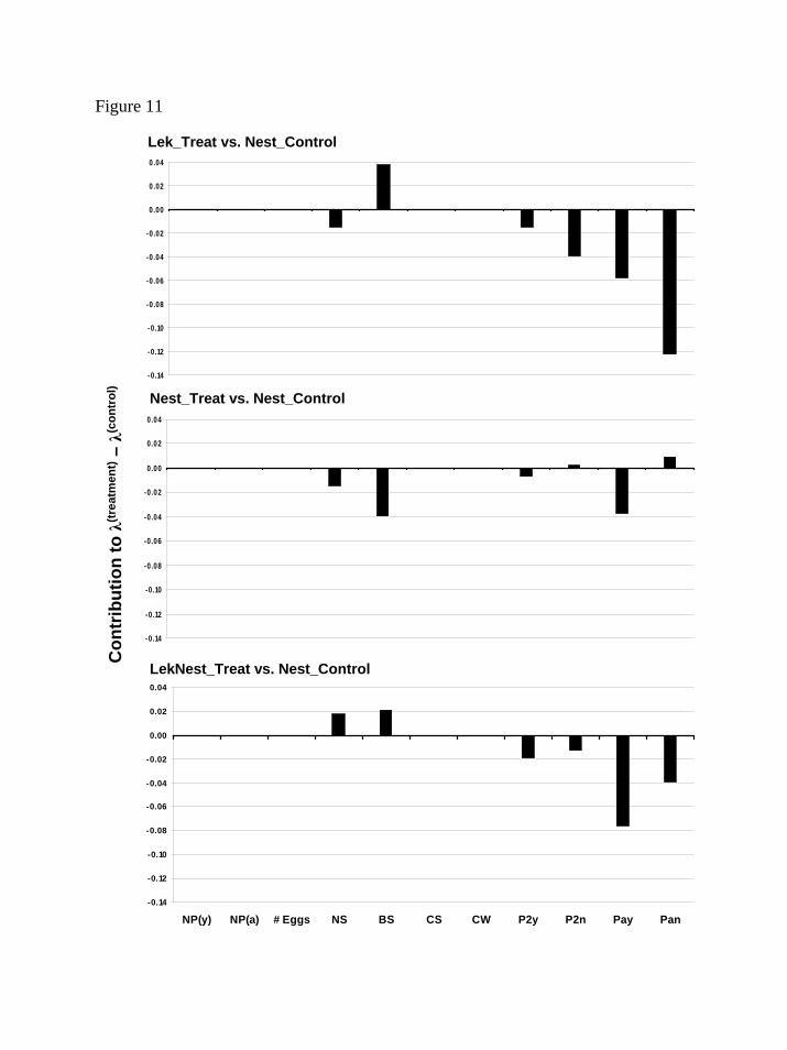
-0.14

-0.12

-0.10

-0.08

-0.06

-0.04

-0.02

0.00

0.02

0.04

Lek_Treat vs. Nest_Control

-0.14

-0 .12

-0 .10

-0.08

-0.06

-0.04

-0.02

0.00

0.02

0.04

Nest_Treat vs. Nest_Control

-0.14

-0.12

-0.10

-0.08

-0.06

-0.04

-0.02

0.00

0.02

0.04

NP(y) NP(a) # Eggs NS BS CS CW P2y P2n Pay Pan

LekNest_Treat vs. Nest_Control

Con

trib

utio

n to

λ(tr

eatm

ent)

–λ(

cont

rol)

Figure 11

CHAPTER 3

NATURAL GAS DEVELOPMENT IMPACTS TO GREATER SAGE-GROUSE

POPULATIONS: A SUMMARY OF RESEARCH CONDUCTED IN WESTERN WYOMING

WITH THOUGHTS ON MANAGEMENT AND FUTURE RESEARCH OPTIONS.

Natural gas development in western North America has been escalating since the 1960s (Braun

et al. 2002, Connelly et al. 2004), and the current U.S. political climate suggests that development of

domestic fossil fuels reserves will continue to expand through the first half of the 21st century. Given

that reducing the U.S. dependence on foreign sources of petroleum, the use of natural gas (versus oil or

coal) as an energy source has air quality benefits, and the protection of natural ecosystems and the

wildlife that depend on these habitats are of equivalent importance to the future of the country, it

behooves us to develop extractive techniques that minimize extraneous consequences. This study

concentrated on natural gas development impacts to a single species, but the results imply potential

responses of an array of wildlife populations dependent on sagebrush-dominated landscapes.

Scientific and anecdotal evidence suggest that sage-grouse (Centrocercus spp.) leks situated

within a developing natural resource field become unoccupied over a relatively short period of time

(Braun et al. 2002, Aldridge and Brigham 2003); however, the specific components of a developing

field that result in declines, as well as the root causes of lek abandonment, remain unidentified.

Remington and Braun (1991) studied the effects of coal mining on breeding greater sage-grouse

(Centrocercus urophasianus) in North Park, Colorado, and theorized that regional distributions were

altered by this disturbance. This displacement theory is supported by several other studies. In

Wyoming, Lyon and Anderson (2003) reported that female greater sage-grouse disturbed on a lek by

road-related activity in natural gas fields moved farther from leks to nest compared to undisturbed

females. Greater sage-grouse in Canada avoided nesting in areas with increased levels of human

development and brooding females avoided areas with increased levels of visible oil wells (Aldridge

2005). Lesser prairie-chickens (Tympanuchus pallidicinctus) in Kansas selected habitats removed from

anthropogenic features (Hagen 2003), and patch occupancy probabilities of Gunnison sage-grouse

(Centrocercus minimus) in Colorado have been positively correlated with distance to roads (Oyler-

McCance 1999). There is also evidence to suggest negative effects at the population scale. Female

greater sage-grouse disturbed by natural gas development during the breeding season had lower nest

initiation rates compared to undisturbed females in Wyoming (Lyon and Anderson 2003), and chick

survival decreased as oil well densities within 1 km of brooding locations increased in Canada

(Aldridge 2005). Hagen (2003) reported that a lesser prairie chicken population subjected to

107

anthropogenic activity in Kansas had population growth rates 21% lower than an undisturbed

population, and suggested that the difference was primarily due to decreased nest success and female

survival in the disturbed area.

I investigated potential impacts of development of natural gas fields to greater sage-grouse

populations in the upper Green River Basin of western Wyoming. The populations and habitats within

this area are currently considered internationally significant strongholds for the species (Connelly et al.

2004). Natural gas development throughout the Intermountain West is occurring primarily within the

sagebrush-dominated landscapes important for sage-grouse survival (Knick et al. 2003). Our objectives

were to investigate several increasingly specific questions: Are breeding greater sage-grouse

populations impacted by natural gas development? What aspects of developing fields are influencing

breeding populations? Are individuals dispersing from natural gas development or are population sizes

declining? Additionally, land management agencies stipulate restrictions on some types of

development during breeding and nesting seasons to protect sage-grouse; so I addressed the adequacy

of these stipulations. I investigated population and individual bird response to natural gas drilling rigs,

producing wells, and main haul roads (i.e., roads accessing at least 5 producing natural gas wells).

I assessed temporal changes in the number of displaying males with respect to distance and

direction from leks to drilling rigs, producing wells, and main haul roads, producing well and main haul

road densities, and traffic activity levels and timing. I also investigated male survival probabilities, lek

tenacity, and habitat selection during the breeding season relative to cumulative levels of gas field

development surrounding leks. My investigation of female habitat selection response to energy

development concentrated on 2 demographic stages, nesting and early brood-rearing (hatch through 2

weeks post-hatch). I examined distances moved between nests in consecutive years, used versus

available nesting and early brood-rearing habitats, and successful (i.e., hatched or survived) versus

unsuccessful nests and broods with respect to differing levels of gas field development. Finally, I used

matrix population modeling and life-table-response procedures (Caswell 1989, 1996) to investigate the

effects of natural gas development on female greater sage-grouse population growth. I compared

populations potentially impacted by natural gas infrastructure during the breeding or nesting season to

non-impacted populations.

Results

Investigating changes in the number of male greater sage-grouse occupying a lek relative to

cumulative gas field development levels using principal components analysis suggested that as the

distance from leks to drilling rigs, producing wells, and main haul roads decreased, and as main haul

108

road densities within 3 km and the number of directions to producing wells within 5 km (i.e., the lek

became more centrally located within the developing field) increased, lek attendance by males

approached zero. The number of males occupying leks within 5 km of drilling rigs declined relative to

non-impacted leks. There did not appear to be visual effects of drilling rigs on lek attendance by males,

but the number of males declined on leks east of drilling rigs (i.e., generally downwind based on

prevailing wind direction). The number of males occupying leks within 3 km of producing wells also

declined. Male lek attendance declined if well densities within 3 km of the lek exceeded approximately

5 wells and if producing wells within 5 km occurred in over half of the directions from leks. Male lek

occupancy also declined on leks within 3 km of main haul roads. Rates of decline increased as traffic

volumes increased, and vehicle activity on roads during the daily strutting period (i.e., early morning)

had a greater influence on attendance compared to roads with no vehicle activity during early morning.

Probabilities of adult male desertion (i.e., males captured from a particular lek and not

documented on that lek following capture) were higher from leks impacted by at least 1 gas-field-

related factor compared to non-impacted leks, and male breeding season survival probabilities were

lower for lightly impacted (i.e., leks impacted by 1 or 2 factors) compared to heavily impacted leks (i.e.,

leks impacted by more than 2 factors). Additionally, impacted leks had fewer yearling males trapped

and earlier peak attendance dates compared to non-impacted leks.

Greater sage-grouse nesting sites were close to wells in areas with low well densities compared

to available sites. Temporally, nests were located farther from drilling rigs and gas wells in 2004

compared to available sites, whereas nests were closer to these structures in 2000-2003. Adult females

nested within previously selected nesting areas regardless of changes in gas development levels within

those areas, but nesting yearlings avoided road-related disturbances. Brooding females avoided

producing wells during the early brood-rearing period. The effect of natural gas development on

female population growth was generally negative. There were relatively consistent negative

contributions to population growth from adult and yearling female annual survival, whereas

productivity contributions were generally positive. This suggests that reduced population growth was

attributable to decreased annual survival of both adult and yearling females.

Discussion

The evidence suggests that current natural gas development techniques lead to greater sage-

grouse population declines. Male lek attendance declined as the distance from leks to drilling rigs,

producing wells, and main haul roads decreased and as densities of these features increased. Lek

attendance also declined as traffic volumes and potential for greater noise increased, and when well

109

densities exceeded 1 well per 283 ha within 3 km of leks. Developing natural gas fields simultaneously

consists of all the disturbance factors considered plus others not investigated (i.e., well completion

activity, compressor stations). Greater sage-grouse breeding populations were probably reacting to a

combination of these factors’ effects.

Adult male displacement and low juvenile male recruitment appear to contribute to declines in

the number of breeding males on impacted leks. Additionally, avoidance of gas field development by

predators could be responsible for decreased male survival probabilities on leks situated near the edges

of developing fields (i.e., lightly impacted leks). Although site-tenacious adult females did not engage

in breeding dispersal in response to increased levels of gas development, subsequent generations

avoided gas fields, as suggested by the temporal shift in nesting habitat selection and differences in

habitat selection by yearling and adult females. This suggests that the nesting population response is

delayed avoidance of natural gas development. The results suggest that male and female greater sage-

grouse displacement from developing natural gas fields contributes to breeding population declines.

Population growth differences between impacted and non-impacted populations suggest that

natural gas development negatively impacts population growth of females. Most of the variability in

population growth was explained by lower annual survival buffered to some extent by higher

productivity in impacted populations. Development effect was especially noticeable on annual survival

of nesting adults. Seasonal survival differences suggested a lag period between when an individual was

impacted by disturbance and when survival probabilities were influenced. Individuals were influenced

by natural gas development primarily during the breeding and nesting periods, while differential

survival occurred primarily during the early brooding and summer periods. Impacted and non-impacted

populations summered in the same general areas, and predators were responsible for most summer

mortalities. Increased predation probabilities during the summer suggest increased exposure, possibly

through a change in foraging behavior (i.e., spending more time feeding), habitat selection (i.e.,

selecting areas with greater food resources and reduced cover), or self-preservation behavior (i.e.,

reduced alertness).

The evidence suggests that breeding population declines and eventual extirpation of leks near

disturbances resulted from both displacement and decreased survival. Regional greater sage-grouse

population levels as well as population distributions are likely to be influenced negatively by

development of natural gas fields.

110

Management Considerations

To protect breeding greater sage-grouse, the Bureau of Land Management (2000) stipulates the

following restrictions to development: (1) no surface disturbance with 0.4 km of a lek; (2) no activity

within a 0.8-km radius of active leks between 0000 and 0900 hrs during the breeding season; (3) no

construction or drilling activities during the breeding season within 1.6 km of active leks. To protect

nesting and brooding females, the Bureau of Land Management (2000) stipulates that gas field related

construction activities will be restricted during the breeding and nesting seasons in suitable nesting

habitat within 3.2 km of active leks; a suitable habitat designation requires that an active nest be located

during an on-site review of the proposed development area. This study suggests that current

stipulations are inadequate to maintain greater sage-grouse breeding populations within natural gas

fields. The effect-distance from disturbance sources to leks during the breeding season could be

conservatively estimated at 3-5 km, especially if that source was located where sound propagation

towards a lek was intensified by environmental factors (i.e., prevailing wind direction). Therefore,

sound muffling devices installed on noisy gas field structures could reduce the negative consequences

on breeding grouse. Declines in lek attendance were positively correlated with traffic levels and

vehicular activity during the daily strutting period. Reducing overall traffic volumes (i.e., offsite

condensate collection facilities, car-pooling) and isolating the timing and location of traffic disturbance

(i.e., restricting travel to and from the gas field to 1 major artery, enforcing daily travel timing

restrictions) within gas fields could reduce road effects.

Barring direct disturbance resulting in nest abandonment, the stipulation (Bureau of Land

Management 2000) aimed at protecting nesting females protects only philopatric individuals. Basing

designations on habitat conditions rather than habitat occupancy could assist in maintaining nesting

areas. Although adequate buffer distances are unknown, our findings suggest that areas designated as

suitable breeding habitats (Connelly et al. 2000) within 5 km of known leks (Holloran and Anderson

2005) need to be protected and buffered from gas field development. Additionally, nesting females

avoided areas with high well densities. Although actual densities resulting in avoidance are unknown,

this result suggests that 16 ha well-spacing excludes nesting females. Because a developing natural gas

field consists of multiple disturbance sources, all of which potentially influence greater sage-grouse

leks and nests, managers need to ensure that all potential factors are addressed concomitantly.

Our results suggest that protection and enhancement of greater sage-grouse populations

inhabiting areas adjacent to natural gas fields could be required to maintain regional population levels.

Off-site mitigation measures aimed at minimizing the negative consequences of natural gas

development on regional populations imply the need for a refugia approach to species conservation. By

111

protecting and enhancing reservoir populations surrounding developing gas fields, greater sage-grouse

could be present to re-colonize the field following reclamation. However, managers need to ensure that

these reservoir populations are protected through the life-expectancy of the developing field (minimum

life-expectancy of the Pinedale Anticline natural gas field has been estimated at 59 years; Bureau of

Land Management 2000). We suggest delaying development of natural gas fields surrounding the

original field until populations within the original field following reclamation are substantial enough to

re-colonize subsequently developed fields. The staggered development of gas fields across a landscape

could not only ensure refugia for wildlife, but could ensure long-term financial stability for states

dependent on fossil fuels generated revenue (at least until alternatives to fossil fuels are developed).

Research Needs

Results from this study identified several questions for future research. Of utmost importance is

determining natural gas development options that reduce detrimental consequences to greater sage-

grouse populations. An investigation of greater sage-grouse population and individual response to

differing development strategies in an experimental context is required for accurate conclusions. The

study design would need to ensure both adequate pre-treatment data for development threshold

identification and spatial independence to guard against potential dispersal consequences. Investigating

potential development options in this manner will require substantial cooperation between researchers,

land managers, and operators.

Research investigating yearling responses to a developing gas field would improve our

understanding of regional consequences. For example: what proportion of the yearling male

population does not breed? What is the spatial extent of the area searched by disturbed yearling males

prior to establishing a territory on a lek (spatial extent of gas field influence)? Is territorial

establishment timing and survival of yearling males influenced by displacement? Future research

should further address potential impacts to the yearling female cohort. In addition to the questions

asked concerning yearling males, information relative to female seasonal habitat selection and

productivity is needed. What is the proportion of the yearling female population displaced from their

natal nesting or natal brooding areas? Are vital rates (i.e., survival, nesting initiation and success

probabilities, and chick productivity rates) of the yearling females displaced from their natal lek,

nesting, or brooding areas negatively influenced?

Research investigating the consequences of dispersal is also needed. If the majority of displaced

adult and recruited yearling males are establishing on non-impacted leks surrounding the developing

gas field, and the eventual nesting population response is avoidance of natural gas development,

112

populations surrounding the gas field may be artificially high. Are density-dependant processes

occurring that affect greater sage-grouse survival, breeding potential, and productivity in sagebrush

habitats with potentially artificially high populations adjacent to natural gas fields (LaMontagne et al.

2002)? And do these processes influence the ability to conduct off-site mitigation for natural gas

development?

Finally, investigating long-term impacts of natural gas development is warranted. Do breeding

populations reoccupy abandoned leks after development stages are completed and the field enters

primarily production phases (i.e., determination of a gas field’s temporal extent of influence)? Braun et

al. (2002) reported that 2 leks in Canada remained inactive for ≥10 years after gas or oil well site

reclamation; however, Remington and Braun (1991) suggested that 2 leks where coal mining activity

potentially caused substantial male lek attendance declines in the early 1980s recovered to some extent

over a 5-year period following the reduction in mining activity in 1985. Research investigating

potential cumulative effects (i.e., influence of gas development on predator core-area use patterns,

produced water and West Nile Virus prevalence [Naugle et al. 2004]) of natural gas field development

is additionally needed. These studies are required to accurately evaluate mitigation options.

Literature Cited



Canada.








United States Bureau of Land Management, Pinedale, WY, USA.

Caswell, H. 1989. Analysis of life table response experiments I. decomposition of effects on

population growth rate. Ecological Modelling 46:221-237.

Caswell, H. 1996. Analysis of life table response experiments II. alternative parameterizations fro

size- and stage-structured models. Ecological Modelling 88:73-82.

113


Greater Sage-grouse and sagebrush habitats. Western Association of Fish and Wildlife


Connelly, J. W., M. A. Schroeder, A. R. Sands, and C. E. Braun. 2000. Guidelines to manage sage










LaMontagne, J. M., R. L. Irvine, and E. E. Crone. 2002. Spatial patterns of population regulation in

sage grouse (Centrocercus spp.) population viability analysis. Journal Animal Ecology 71:672-

682.










Colorado. Proceedings, Issues and Technology in the Management of Impacted Western

Wildlife. Thorne Ecological Institute 5:128-132.

114

A1

APPENDIX A

Abridged Title. Greater Sage-Grouse Nest Distribution

SPATIAL DISTRIBUTION OF GREATER SAGE-GROUSE NESTS IN RELATIVELY

CONTIGUOUS SAGEBRUSH HABITATS

MATTHEW J. HOLLORAN, Wyoming Cooperative Fish and Wildlife Research Unit, University of

Wyoming, Department 3166, Laramie, WY 82071. 307 766 2091 (voice); 307 766 5400 (fax);

[email protected] (e-mail).

STANLEY H. ANDERSON, Wyoming Cooperative Fish and Wildlife Research Unit, University of

Wyoming, Department 3166, Laramie, WY 82071.

Abstract. Degradation of nesting habitat has been proposed as a factor contributing to Greater

Sage-Grouse (Centrocercus urophasianus) population declines throughout North America. Delineating

suitable nesting habitat across landscapes with relatively contiguous sagebrush cover is difficult but

important to identify areas for protection. We used radio-telemetry to locate Greater Sage-Grouse nests

in relatively contiguous sagebrush habitats in Wyoming to investigate the spatial arrangement of nests

relative to lek and other nest locations. Nest distributions were spatially related to lek location within 3

and 5 km of a lek, and a 5-km buffer included 64% of the nests. There was no relationship between lek

size and lek-to-nest distance, suggesting that accurate population trend evaluation might require lek

surveys in addition to lek counts. Closest known lek-to-nest distance was greater for successfully

hatched compared to destroyed nests, and closely spaced nests tended to experience lower success and

have higher probabilities of both nests experiencing the same fate compared to isolated nests,

suggesting that a mechanism of enhanced prey detection occurred at higher nest densities. A low

probability that a given individual’s consecutive-year nest spacing occurred randomly suggested nesting

site-area fidelity. Although a grouped pattern of nests occurred within 5 km of a lek, the proportion of

nesting females located farther than 5 km could be important for population viability. Managers should

limit strategies that negatively influence nesting habitat regardless of lek locations, and preserve

adequate amounts of unaltered nesting habitat within treatment boundaries to maintain nest dispersion

and provide sites for philopatric individuals.

A2

Key words: Centrocercus urophasianus, fidelity, lek-to-nest distance, nest distribution, nest

spacing, Greater Sage-Grouse, Wyoming.

INTRODUCTION

Shrubland and grassland bird species are declining faster than any other group of species in North

America, primarily due to human caused destruction and degradation of their habitats (i.e., livestock

grazing, land conversion, natural resource development, habitat treatment; Knick et al. 2003).

However, because of the perceived uniformity of relatively contiguous sagebrush dominated and

grassland ecosystems, accurate delineation of areas supporting habitat conditions seasonally required by

obligate bird species across landscapes is difficult. Greater Sage-Grouse (Centrocercus urophasianus)

currently occupy 56% of their pre-European settlement distribution (Schroeder et al. 2004), and

breeding populations throughout North America are two to three times lower than those during the late

1960s (Connelly et al. 2004); the loss of suitable nesting habitat may be contributing to these declines

(Crawford et al. 2004). Because recognizing suitable nesting areas based on habitat structural cues

throughout the core of the species’ range is often difficult, managers have long used leks to identify

nesting habitats. The 1977 Sage-Grouse habitat management guidelines (Braun et al. 1977) recommend

protecting all areas within 3 km of a lek as potential nesting habitat. The current management

guidelines (Connelly et al. 2000) suggest using leks as focal points for nesting habitat management

efforts, and recommend protecting the sagebrush (Artemisia spp.) overstory and herbaceous understory

within 3.2 km of occupied leks in areas with uniformly distributed habitats. In non-uniformly

distributed habitats, the current guidelines (Connelly et al. 2000) recommend protecting the area within

5 km of a lek.

The spatial dependence between an organism and a suspected influential component of its

environment is a fundamental question in ecology (Rossi et al. 1992). The development of theories on

spatial organization revolves around the discovery of patterns (Levin 1992), and because patterns

change as a function of spatial resolution, the scale of observation can alter the description of species

distributions (Trani 2002). Although Wakkinen et al. (1992a) concluded that the distribution of Greater

Sage-Grouse nests was random with respect to lek location because of no statistical differences between

closest known lek-to-nest and lek-to-random point distances in Idaho, the spatial scale of interest was

restricted to the study area. If the area of interest was expanded, at some spatial scale a non-random

distribution of nests relative to lek location should have become discernable. The spatial scale at which

a discernable pattern exists (where the distribution of nests become non-random with respect to lek

location) could be used to quantify the area surrounding an occupied lek where female Greater Sage-

A3

Grouse are likely to select a nesting site; this could be used by land managers as a preliminary

designation of potential nesting habitat in areas where differentiating habitats is difficult.

Several theories exist concerning the relationship between the probability of hatching success

and nest placement relative to the location of the lek, another individual’s nest, and an individual’s

previous nesting location. Bergerud (1988) suggested that, to lower nest depredation probabilities,

nesting females should avoid leks to minimize disturbance by males and evade increased predator

activity associated with leks. Mean lek-to-nest distance was greater for successful compared to

unsuccessful Greater Sage-Grouse nests in California (Popham and Gutierrez 2003). In vulnerable

species, the optimal dispersion pattern for avoiding detection in continuous habitats should be towards

well-spaced, solitary individuals (Taylor 1976, Andersson and Wiklund 1978, Bergerud and Gratson

1988). Niemuth and Boyce (1995) suggested that nest detection by predators was greater at high-

density compared to low-density artificial Greater Sage-Grouse nest situations in Wyoming. Fidelity to

nesting areas could have potential advantages, including increased familiarity with a site and its

predators and competitors and reduced dispersal costs (Bergerud and Gratson 1988). Fischer et al.

(1993), in Idaho, reported that distances between Greater Sage-Grouse nests in consecutive years

represented 3.5% of median annual movements, suggesting fidelity for specific nesting areas.

Because of Greater Sage-Grouse population declines (Connelly et al. 2004, Schroeder et al.

2004) and the numerous potential deleterious impacts occurring to nesting habitats (Braun 1998),

identifying potential nesting areas and characteristics favorable for increased productivity could be

important for population sustainability. We used Greater Sage-Grouse nest sites located in relatively

contiguous sagebrush habitats in central and western Wyoming to investigate the spatial arrangement of

nests relative to lek and other nest locations. Our primary objective was to determine the spatial scale

at which nests become non-randomly distributed around leks. As predicted by the optimal nest

dispersion pattern theory (Taylor 1976, Andersson and Wiklund 1978, Bergerud and Gratson 1988), we

hypothesized that lek-to-nest distances, and thus the distance from a lek where a non-random nest

distribution pattern was detected, would be positively correlated with lek size. We further hypothesized

that hatching success probabilities would be positively correlated with lek-to-nest distances, that

isolated nests would experience higher rates of success than closely-spaced nests, and that females

would exhibit fidelity to specific nesting-areas.

A4

METHODS

STUDY AREA

We studied Greater Sage-Grouse at seven sites located in central and southwestern Wyoming in 1994-

2003 (detailed description in Holloran et al. in press). Although habitat manipulations (i.e., fire,

herbicide application) and livestock grazing occurred in the areas (Holloran 1999, Lyon 2000, Slater

2003, Kuipers 2004), large scale habitat conversions (i.e., cropland, human dwellings) were not present,

and the areas were dominated by uniformly distributed sagebrush habitats. Areas fragmented by natural

gas development were removed from consideration. Vegetation was dominated by Wyoming big

sagebrush (A. tridentata wyomingensis). Black sagebrush (A. nova) and low sagebrush (A. arbuscula)

were located on relatively flat terrain in shallow soils, basin big sagebrush (A. t. tridentata) and silver

sagebrush (A. cana) were located in deeper soils, and mountain big sagebrush (A. t. vaseyana) was

found in mixed stands with Wyoming big sagebrush at higher elevations. Rabbitbrush (Chrysothamnus

spp.), black greasewood (Sarcobatus vermiculatus), antelope bitterbrush (Purshia tridentata),

snowberry (Symphoricarpos spp.), and serviceberry (Amelanchier alnifolia) were interspersed

throughout study areas. Dominant grasses included bluebunch wheatgrass (Pseudoroegneria spicata),

western wheatgrass (Agropyron smithii), junegrass (Koeleria pyramidata), needlegrasses (Stipa spp.),

bluegrasses (Poa spp.), Indian ricegrass (Oryzopsis hymenoides), Idaho fescue (Festuca idahoensis),

and cheatgrass (Bromus tectorum). Common understory forbs included lupine (Lupinus spp.), phlox

(Phlox spp.), buckwheat (Eriogonum spp.), common dandelion (Taraxacum officinale), milkvetch

(Astragalus bisulcatus), sandwort (Arenaria capillaris), and several species of Asteraceae.

FIELD TECHNIQUES

Female Greater Sage-Grouse were captured on and near leks each year from mid-March through April

by spot-lighting and hoop-netting (Giesen et al. 1982, Wakkinen et al. 1992b). Each captured female

was classified as a juvenile (first breeding season) or adult (≥ second breeding season) based on the

shape of the outermost wing primaries (Eng 1955). Radio transmitters were secured to females with a

PVC-covered wire necklace (Advanced Telemetry Systems Inc. [ATS], Isanti, MN). Transmitters used

between 1994 and 1997 weighed 12 g and had a battery life expectancy of 305 days. In 1998,

transmitters weighing 25 g with a battery life expectancy of 610 days were developed by ATS and used

between 1998 and 2003.

Hand-held receivers and Yagi antennas were used to monitor radio-marked females at least

twice weekly through pre-laying (April) and nesting (May-June). Nests of radio-marked birds were

located by circling the signal source until females could be directly observed. Nest locations were

A5

recorded in Universal Transverse Mercator (UTM) coordinates using a hand-held 12 channel Global

Positioning System (GPS; Garmin 12; Garmin International, Olathe, KS) or 7.5 minute topographic

maps (US Geological Survey, Denver, CO). We wore rubber boots while confirming nest locations to

reduce human scent, and monitored incubating females after nest identification from a distance of >60

m to minimize the chance of human-induced nest predation or nest abandonment. Nest fate (successful

or unsuccessful) was recorded when radio monitoring indicated the female had left the area. Nests were

considered successful if at least one egg hatched, indicated by presence of detached eggshell

membranes (Wallestad and Pyrah 1974). Unsuccessful hens were monitored twice-weekly to detect

renesting attempts.

STATISTICAL ANALYSES

The spatial scale at which nests became associated with lek location was assessed using Chi-square

tests with continuity corrections (due to sample sizes <25 in certain instances; Dowdy and Wearden

1991). We compared the number of nests (observed locations) to the number of expected points

(assuming a uniform distribution) occurring within 0.5-km bands radiating from the lek. Lek-to-nest

distance was estimated from the lek-of-capture. Because repeated anthropogenic disturbance near a lek

during the breeding season may influence how far a female moves from the lek to nest (Lyon and

Anderson 2003), we excluded any female captured on a lek ≤500 m from a maintained road or other

anthropogenic disturbance source (e.g., natural gas wells; n = 9 leks). Due to a potential lack of

independence, all re-nests (n = 19) and nests from the same individual in years following her first

identified nest (n = 78) were omitted from the lek association analysis. Because each successive 0.5-

km band radiating from the lek encompasses more total area (e.g., 0 to 0.5 km band = 79 ha, 0.5 to 1

km band = 236 ha, 1 to 1.5 km band = 393 ha), the number of expected nests per 0.5-km band will

increase proportionally to the amount of area included in each band. Therefore, using the spatial scale

required to encompass all nests could result in an expected distribution biased away from the lek. We

calculated the total spatial area to consider for the analysis using the upper limit of the 90% confidence

interval around the mean number of nests within each 0.5-km band. We truncated the spatial area of

interest at the point where all successive bands contained fewer nests than designated by this upper

limit (hereafter referred to as the truncated area). Nests situated outside the truncated area (n = 59)

were removed from the analysis. Expected numbers of nests within 0.5-km bands were estimated

assuming a uniform distribution within the truncated area. Given our trapping protocol, nesting (versus

breeding) females could have been radio-tagged (especially those individuals captured later in the

breeding season) which could result in nest distributional estimations biased towards the lek. To test

A6

for this possibility, we removed all individuals radio-tagged later than the median annual date-of-

capture and compared proportional nest numbers per 0.5-km band between this reduced and the full

data sets.

Linear regression was used to evaluate the relationship between lek-to-nest distances and lek

size. Annual median and mean lek-to-nest distance by lek (independent variable) were calculated using

all nests of females captured from a given lek during a given year. To ensure a relatively accurate mean

lek-to-nest distance estimate, only lek years with ≥5 identified nests were used (n = 26). Lek size

(dependent variable) was estimated as the maximum number of males counted during the breeding

period and lek-to-nest distance was estimated from the lek-of-capture. Lek counts were conducted by

researchers according to standardized methods outlined by the Wyoming Game and Fish Department’s

(WGFD) Sage-Grouse technical committee (WGFD, Cheyenne, WY; Connelly et al. 2003).

Separate-variance, two-sample t-tests (Dowdy and Wearden 1991) were used to compare mean

lek-to-nest distance differences between successful and unsuccessful nests. In contiguous habitats,

females may nest closer to a lek other than where bred (i.e., lek-of-captured; Wakkinen et al. 1992a)

and success probabilities may be influenced by the proximate lek; therefore, lek-to-nest distance was

estimated from the closest known lek (versus the lek-of-capture) for this analysis. Radio-marked

individual females dispersing long distances from the lek-of-capture could be difficult to locate, and

thus located late during incubation stages. Because nests located later in the nesting cycle have fewer

days at risk of nest failure (Nur et al. 2004), apparent nest success probabilities could be biased by

distance. To investigate the possibility of distance-biased apparent success probabilities, we compared

the total number of days successfully nesting females were documented incubating (i.e., number of days

between nest identification and hatch) and closest known lek-to-nest distances using Pearson’s

correlation coefficients (r).

The influence of nest density on the probability of nest success was evaluated using nest spacing

distances (i.e., known nest-to-nest distances). To ensure relatively representative nest-to-nest distance

estimations, we included only those nests located within the truncated area, and used lek years with ≥10

individual identified nests (n = 9 lek years; mean female sample by lek = 13 [range 10 to 20 females]).

Individual nests (n = 114) and nest pairs (n = 86) were classified into 0.5-km categories based on

distance to closest known nest and distance between nest pair, respectively (i.e., nest-to-nest distance 0

to 500 m, 501 to 1000 m). Expected probabilities of nest success were estimated using overall nest

success probabilities (all nests) and expected probabilities of nest pairs experiencing the same fate were

estimated as chance (50%); apparent nest success probabilities (observed probabilities) were compared

to expected probabilities by category and inclusively using Chi-square tests with continuity corrections

A7

(Dowdy and Weardon 1991). Because our nest density estimates could have been influenced by lek

size or trapping effort, we investigated relationships between mean nest-to-nest distances and maximum

number of males and total number of identified nests by lek year using Pearson’s correlation

coefficients.

To examine female fidelity to specific nesting areas, we compared distances between

consecutive-years’ nests to distances expected given random between-year nest placements within the

truncated area. We generated a uniform distribution of random points (numerically equal to the number

of nests; n = 78) within the truncated area using Animal Movement (Hooge and Eichenlaub 1997) in

ArcGIS 9 (Environmental Systems Research Institute, Redlands, CA) and calculated the distance

between each point and a randomly chosen additional point. The point-to-point distances were binned

into 0.5-km categories and a probability distribution was produced based on the cumulative number of

point-to-point distances occurring within each 0.5-km band radiating to the maximum possible distance

between two points (i.e., diameter of the truncated area). We used this random point spacing

probability distribution to assess the probability that mean and median consecutive-year nest-to-nest

distances were random. Additionally, Mann-Whitney U-tests (Sokal and Rohlf 1995) were used to

investigate median consecutive-year movement differences between adult and yearling, and both 1st and

2nd year successful and unsuccessful females. Values reported in the results section are medians and

means (± standard error). All statistical procedures were performed with MINITAB 13.1 (Minitab Inc.,

State College, PA). Statistical significance was assumed at α ≤ 0.05, and tendencies were assumed at α

≤ 0.10.

RESULTS

Between 1994 and 2003, we located 437 Greater Sage-Grouse nests of females captured from 30

relatively undisturbed leks throughout central and western Wyoming. Median and mean lek-of-capture

to nest distance for all nests was 3506 and 4700 m (± 204 m), respectively (range 282 m to 27.4 km).

Mean number of nests per 0.5-km band was 6.2 (± 1.2), and suggested that the area of interest should be

truncated at 8.5 km (Fig. 1). Twenty-six leks ranging in size from 9 to 102 males were used for the

spatial distribution relative to lek size analysis. After removing all nests of unknown fate and

abandoned nests, 415 total nests (187 successful; 228 unsuccessful) and 384 nests within 8.5 km of the

closest known lek (168 successful; 216 unsuccessful) were used for the nest fate analysis. We used 78

consecutive-year pairs of nests for the nesting-area fidelity analysis.

Significantly greater numbers of nests than expected occurred in all 0.5-km bands ≤3 km of the

lek (χ21 ≥ 7.6; P < 0.01); in all bands between 3 and 5 km of the lek, the number of nests did not differ

A8

from expected (χ21 ≤ 1.8; P > 0.17); and there were significantly fewer nests than expected (χ2

1 ≥ 4.0; P

< 0.05) within all bands between 5 and 8.5 km of the lek (Fig. 1). Forty-five and 64% of all nests (n =

437) were within 3 and 5 km of the lek, respectively. After removing all nests of individuals radio-

tagged later than the median annual date-of-capture, we found that proportional differences were ≤2%

except the 1 to 1.5-km band, where proportional nest numbers were 5% lower for the reduced compared

to full data set. However, the reduced number of nests within the 1 to 1.5-km band was still greater

than expected given a uniform distribution (χ21 = 12.3; P < 0.01). There was no relationship between

lek size and median (R2 = 1.0%) or mean (R2 = 0.2%) lek-to-nest distance.

Closest known lek-to-nest distance was not highly correlated with the number of days females

were documented incubating (r = 0.22), suggesting no distance-bias associated with apparent success

probability estimates; therefore, apparent nest success probabilities were used for fate analyses. For all

nests, mean closest known lek-to-nest distance was significantly greater for successful (3978 m)

compared to unsuccessful (3338 m) nests (t334 = 2.0; P = 0.04). However, comparing successful and

unsuccessful nests within 8.5 km of a lek indicated no differences in mean lek-to-nest distances

(successful 3087 m; unsuccessful 2952 m; t358 = 0.6; P = 0.53). We additionally investigated hatching

success probabilities for nests within 5 km of a lek post-hoc, and found no differences in mean lek-to-

nest distances between successful (2183 m; n = 133) and unsuccessful (2092 m; n = 174) nests (t284 =

0.6; P = 0.52).

Inclusively, nest success probabilities for nests categorized by distance to another known nest

did not differ from success probabilities expected by overall nest success rates (45%; χ24 = 5.9; P =

0.21). Additionally, inclusive probabilities of both nests experiencing the same fate did not differ from

probabilities expected by chance (50%; χ24 = 4.7; P = 0.32). However, nests located ≤1 km from

another known nest (n = 58) tended to have lower than expected probability of success (cumulative

28%; χ21 = 3.5; P = 0.06), and the probability of both nests (n = 38 pairs) experiencing the same fate

(cumulative 71%) tended to be greater than expected by chance (χ21 = 3.0; P = 0.08). Nest success

probabilities (cumulative 41%) for nests >1 km from another known nest (n = 56) did not differ from

overall nest success probabilities (χ21 = 0.1; P = 0.73), and paired fate for nests >1 km (cumulative 56%;

n = 48 pairs) did not differ from chance (χ21 = 0.4; P = 0.61). Mean nest-to-nest distances by lek year

were not highly correlated with lek size (r = 0.37), but were highly correlated with female sample size

(r = 0.75). The relationship between mean nest-to-nest distance and female sample size was positive

(i.e., longer mean nest-to-nest distances for leks with larger sample sizes). There was low correlation

between lek size and sample size (r = 0.27).

A9

Median and mean distance between consecutive-year nests for all females was 415 and 740 m

(± 97 m), respectively (range 40 to 4966 m). Based on the cumulative probability distribution assuming

random annual nest placement within the truncated area, the probability that a female selected a nest

site within 0.5 km from the previous year’s nest was 1.2% (median distance probability); the probability

that between year nest movements were ≤1 km was 2.6% (mean distance probability). Median

distances moved between consecutive-year nests by adults (391 m; n = 50) and yearlings (540 m; n =

28) were similar (U = 832; P = 0.17). Females moved significantly farther (U = 825; P < 0.01) to

subsequent-year nests following an unsuccessful nesting attempt (median = 512 m; n = 40) compared to

movements following a successful nesting attempt (median = 283 m; n = 28). However, there was no

relationship between distance moved and subsequent-year nest success for all nests (2nd year successful

median = 382 m, n = 27; 2nd year unsuccessful median = 415 m, n = 41; U = 625; P = 0.37) or for

females whose first documented nest was unsuccessful (2nd year successful median = 497 m, n = 15; 2nd

year unsuccessful median = 532 m, n = 25; U = 208; P = 0.58).

DISCUSSION

Protection of Greater Sage-Grouse nesting habitat within 3.2 km of occupied leks has been a standard

management recommendation since the 1970s (Braun et al. 1977, Connelly et al. 2000). However,

research in fragmented (Schroeder et al. 1999, Aldridge and Brigham 2001) and contiguous (Bradbury

et al. 1989, Wakkinen et al. 1992a) habitats suggest these recommendations offer limited or

unsubstantiated protection to nesting areas. Bradbury et al. (1989) and Wakkinen et al. (1992a) argue

that females select nest sites independent of lek location. However, as the spatial resolution of interest

expands from a lek, a point should be reached where a discernable pattern of nest placement relative to

lek location becomes apparent.

Greater Sage-Grouse nest distributions were grouped relative to lek location at multiple spatial

scales. The question thus becomes, which distance (3 or 5 km) represents the spatial scale that

effectively delineates the amount of area surrounding a lek that encompasses the proportion of nesting

individuals required for population viability? The proportion of nests located within 3 versus 5 km (45

vs. 64%, respectively) suggested that a 5-km buffer around a lek was required to encompass a relative

majority of nests. Additionally, nests located within 1 km of another known nest tended to have lower

success probabilities, suggesting that increased nest densities could negatively influence the probability

of a successful hatch. Given the number of nests relative to the amount of area within 0 to 3 km (2827

ha) versus 3 to 5 km (5027 ha) from a lek (Fig. 1), nest densities decreased as lek-to-nest distance

A10

increased. This further indicates that a 5-km buffer could be required, and suggests that the area

between the 3 and 5-km buffers could be especially important.

Although the observed distribution of nests relative to a uniform distribution surrounding a lek

indicated that a pattern of landscape scale spatial association of nests relative to lek location occurred at

5 km, only 64% of the nests were located within this buffer distance. Additionally, lek-to-nest distance

and hatching success probabilities were not related for nests within 5 km, but were positively correlated

for all nests, suggesting increased success probabilities for individuals nesting far from a known lek.

Survival of nests located far from a lek may be influenced by factors other than lek proximity

(Moynahan 2004). However, regardless of the mechanism responsible for increased success

probabilities, the segment of the population nesting beyond the 5-km distance may be important for

population sustainability. Our results suggested that 5-km buffers around leks located within relatively

contiguous habitats could be used by land managers as a preliminary designation of potential nesting

areas. Additionally, nesting habitats located beyond 5 km from a lek may be important for population

viability, suggesting protection (Connelly et al. 2000) should also be afforded to these areas.

Our trapping protocol potentially resulted in the capture of nesting (versus breeding) females

within approximately 1 to 2 km (typical area trapped) of the lek. Although statistical results were not

influenced, this potential bias suggested nest numbers within 0 to 3 km were overestimated. The lack

of a relationship between lek-to-nest distances and documented incubation duration suggested that there

was no distance bias associated with our fate analyses. Mean nest-to-nest distance correlations by lek

year suggested no nest density estimate bias associated with lek size, but a potential bias associated

with female sample size. However, the relationship between nest spacing and sample size was positive,

opposite of the relationship expected if trapping effort influenced nest density estimates.

The mutual avoidance hypothesis (Taylor 1976, Andersson and Wiklund 1978, Bergerud and

Gratson 1988) predicts that females should disperse nests to decrease detection probabilities. Our

results suggest that Greater Sage-Grouse nests located relatively near (within 1 km) another known nest

tended to be less likely to successfully hatch, supporting this hypothesis. Additionally, lek-to-nest

distances were not related to lek size, suggesting a negative correlation between nest spacing and the

number of females breeding on a lek. Theoretically, nest densities would eventually reach a threshold,

suggesting that the spatial association between nest and lek location could be a mechanism restraining

maximum lek size and leading to range expansion during population increases. Research in Minnesota

suggested that, during a population increase, nest-spacing tendencies of greater prairie chickens

(Tympanuchus cupido pinnatus) resulted in formation of new leks rather than changes in mean number

of males per lek (Bergerud and Gratson 1988). Given that maximum lek size could be constrained by

A11

female nest spacing tendencies, the number of males using a lek may be influenced by parameters other

than population size, and new or historical (unoccupied) leks could become active during population

increases. The current Sage-Grouse management guidelines recommend using annual lek counts to

assess numerical trends in breeding population levels (Connelly et al. 2000). Our results suggest that

surveys for new leks and monitoring of historical (unoccupied) leks in addition to annual lek counts

could be important for accurate population trend evaluation.

Bergerud (1988) hypothesized that leks act as predator attractants and nesting females should

avoid leks to improve hatching probabilities, an idea supported by research in California (Popham and

Gutierrez 2003). Although closest known lek-to-nest distances did not influence hatching success for

Greater Sage-Grouse nests within 8.5 km, there was a positive correlation between distance and success

probabilities for all nests, suggesting increased success rates for nests >8.5 km from a lek (61% success

>8.5 km, 44% success ≤8.5 km). It is probably unreasonable to assume that leks acted as predator

attractants out to 8.5 km, and that decreased nesting success probabilities were being caused by

increased predator numbers within this area. However, the development of prey detection enhancing

behaviors by those predatory individuals residing within the truncated region could be possible.

Locally increased predation could be explained through the development of a search image (Pietrewicz

and Kamil 1981, Allen 1989) or reduced search rate (i.e., predators enhance cryptic prey detection

probabilities by spending more time searching a particular area; Guilford and Dawkins 1987). Pairs of

nests spaced relatively closely within 8.5 km of a lek tended to experience the same fate more

frequently than was expected by chance, suggesting area-concentrated search and enhanced prey

detection (Niemuth and Boyce 1995) and supporting the idea of behavioral changes by predators. Our

results suggest that a mechanism of enhanced prey detection occurs at higher nest concentrations, and

that increased nest densities could result in increased nest depredation probabilities.

Quantifying fidelity to a specific nesting area is difficult (Greenwood and Harvey 1982), given

that female Greater Sage-Grouse are probably not territorial (Schroeder et al. 1999) and do not select

the same shrub for nesting in consecutive years (i.e., Fischer et al. 1993 and this study). Fischer et al.

(1993) used a comparison between consecutive-year nest and annual straight-line movement distances

to suggest that females in Idaho exhibited fidelity for specific nesting areas. However, seasonal

movements are generally in response to changing habitat requirements (Patterson 1952), which in our

study sites resulted in movements between distinct areas that provided resources. Thus, movements

between seasonal ranges might not accurately reflect expected movements within a specific habitat type

in Wyoming. We chose to investigate the question of nesting-area fidelity by creating a probability

distribution with the assumption of random between year nest placement within 8.5 km of a lek. The

A12

probability that observed consecutive-year nest spacing occurred randomly was between 1.2 and 2.6%,

strongly suggesting nesting site-area fidelity. Reasons for site-attachment could include familiarity

with food and cover (refuges from predators) resources, allowing individuals to exploit the area more

efficiently (Greenwood and Harvey 1982).

Our data additionally support Bergerud and Gratson’s (1988) hypothesis that females should

shift nesting areas following an unsuccessful nesting attempt. Unsuccessful females moved farther

between consecutive-year nests in Washington (Schroeder and Robb 2003). Additionally, females

moved 85% farther in Idaho (Fischer et al. 1993) and 81% farther in Colorado (Hausleitner 2003)

following an unsuccessful compared to a successful nesting attempt. However, the relatively long

movements in Wyoming following an unsuccessful nesting attempt did not influence subsequent-year

nesting success probabilities, results similar to those reported from Washington (Schroeder and Robb

2003). The lack of a positive response following a shift in nesting sites could be related to an

individual’s initial unfamiliarity with the new area and the inability to optimally exploit the area’s

resources. However, the consistency of the shifting behavior following an unsuccessful breeding

attempt implies that such breeding dispersal may be advantageous in the long term (Greenwood and

Harvey 1982).

Implicit in the recommendation to use leks as focal points for identifying potential Greater

Sage-Grouse nesting habitat (Connelly et al. 2000) is that nest distributions are related to lek location,

which at some spatial scale will be inherently true. Nest distributions exhibited a grouped pattern

across relatively contiguous sagebrush landscapes within 5 km of a lek; however, the substantial

number of females nesting farther than 5 km from a lek could be important for population viability.

Nest distribution patterns may change as a result of habitat alteration and fragmentation (Schroeder and

Robb 2003), thus a 5-km buffer should be considered relevant only within contiguous sagebrush

habitats. To protect and maintain Greater Sage-Grouse populations residing in relatively contiguous

habitats, our results imply that managers should initially minimize or halt actions that reduce suitability

of nesting habitats within 5 km of a lek. Managers should additionally identify all potential nesting

areas, regardless of proximity to a lek, and consider those for protection. Further, if sagebrush

manipulating proactive treatments are prescribed within potential nesting habitats, treated blocks need

to be relatively small (i.e., less than 54 to 172 ha based on consecutive-year nest movements) and

widely dispersed to provide suitable sites for philopatric individuals and maintain nest spacing.

A13

ACKNOWLEDGMENTS

The Bureau of Land Management, Wyoming Game and Fish Department, U.S. Department of Energy,

Ultra Petroleum, Animal Damage Management Board, Yellowstone-to-Yukon Initiative, EnCana Oil &

Gas Inc., and Cowboy 3-Shot Sage-Grouse Foundation provided financial support for this study. We

thank the following landowners for access: Bates Creek Cattle Company; Bousman Ranch; Carney

Ranch; Ferris Mountain Ranch; Garrott Ranch; Julian Sheep Company; Little Sandy Grazing

Association; Luther Ranch; Miles Cattle Company; Miller Estate; Red Bluff Ranch; Ruby Ranch;

Sealy/Sawyer Ranch; Sommers Ranch; Stone Ranch; and the Three-quarter Circle Ranch. Additional

lek count and nest location data were supplied by B. J. Heath, J. L. Kuipers, A. G. Lyon, and S. J.

Slater. Field assistance was provided by K. D. Downs, M. B. Hicks, R. A. Holloran, B. K. Holtby, M.

A. Kaeminglk, Mr. and Mrs. T. W. Malmberg, T. E. McCollum, R. C. Powell, C. M. Sazama, M. S.

Stotts, C. G. Taber, Mr. and Mrs. N. A. Tratnik, C. T. Weibel, G. L. Wilson, and J. A. Wyllie. Cheney

Flying Service (Casper, WY), France Flying Service (Rawlins, WY), and Mountain Air Research

(Driggs, ID) flew telemetry flights and lek surveys. P. T. McLean (University of Wyoming, Laramie,

WY) provided the abstract translation. D. S. Dobkin, F. G. Lindzey, M. C. Quist, T. E. Rinkes, S. J.

Slater, K. M. Thompson, and 2 anonymous reviewers improved the manuscript greatly.

LITERATURE CITED

Aldridge, C. L., and R. M. Brigham. 2001. Nesting and reproductive activities of Greater Sage-Grouse

in a declining northern fringe population. Condor 103:537-543.

Allen, J. A. 1989. Searching for search image. Trends in Ecology and Evolution 4:361.

Andersson, M., and C. G. Wiklund. 1978. Clumping versus spacing out: experiments on nest

predation in Fieldfares (Turdus pilaris). Animal Behaviour 26:1207-1212.

Bergerud, A. T. 1988. Increasing the numbers of grouse, p. 686-731. In A. T. Bergerud and M. W.

Gratson [eds.], Adaptive strategies and population ecology of northern grouse. University of

Minnesota Press, Minneapolis, MN.

Bergerud, A. T., and M. W. Gratson. 1988. Survival and breeding strategies of grouse, p. 473-577. In

A. T. Bergerud and M. W. Gratson [eds.], Adaptive strategies and population ecology of

northern grouse. University of Minnesota Press, Minneapolis, MN.

Bradbury, J. W., R. M. Gibson, C. E. McCarthy, and S. L. Vehrencamp. 1989. Dispersion of

displaying male Sage Grouse II: the role of female dispersion. Behavioral Ecology and

Sociobiology 24:15-24.

A14

Braun, C. E. 1998. Sage Grouse declines in western North America: what are the problems?


Braun, C. E., T. Britt, and R. O. Wallestad. 1977. Guidelines for maintenance of Sage Grouse habitats.

Wildlife Society Bulletin 5:99-106.


Greater Sage-Grouse and sagebrush habitats. Western Association of Fish and Wildlife

Agencies, Unpublished Report, Cheyenne, WY.

Connelly, J. W., K. P. Reese, and M. A. Schroeder. 2003. Monitoring of Greater Sage-Grouse habitats


University of Idaho, Moscow, ID.

Connelly, J. W., M. A. Schroeder, A. R. Sands, and C. E. Braun. 2000. Guidelines to manage Sage

Grouse populations and their habitats. Wildlife Society Bulletin 28:967-985.

Crawford, J. A., R. A. Olson, N. E. West, J. C. Mosley, M. A. Schroeder, T. D. Witson, R. F. Miller, M.

A. Gregg, and C. S. Boyd. 2004. Ecology and management of Sage-Grouse and Sage-Grouse

habitat. Journal of Range Management 57:2-19.

Dowdy, S. M., and S. Wearden. 1991. Statistics for research. Second edition. John Wiley & Sons,

Inc., New York, NY.

Eng, R. L. 1955. A method for obtaining Sage Grouse age and sex ratios from wings. Journal of

Wildlife Management 19:267-272.

Fischer, R. A., A. D. Apa, W. L. Wakkinen, and K. P. Reese. 1993. Nesting-area fidelity of Sage

Grouse in southeastern Idaho. Condor 95:1038-1041.

Giesen, K. M., T. J. Schoenberg, and C. E. Braun. 1982. Methods for trapping Sage Grouse in


Greenwood, P. J., and P. H. Harvey. 1982. The natal and breeding dispersal of birds. Annual Review

of Ecology and Systematics 13:1-21.

Guilford, T., and M. S. Dawkins. 1987. Search images not proven: a reappraisal of recent evidence.

Animal Behaviour 35:1838-1845.

Hausleitner, D. 2003. Population dynamics, habitat use and movements of Greater Sage-Grouse in

Moffat County, Colorado. M.S. thesis, University of Idaho, Moscow, ID.

Holloran, M. J. 1999. Sage Grouse (Centrocercus urophasianus) seasonal habitat use near Casper,

Wyoming. M.S. thesis, University of Wyoming, Laramie, WY.

A15

Holloran, M. J., B. J. Heath, A. G. Lyon, S. J. Slater, J. L. Kuipers, and S. H. Anderson. In press.

Greater Sage-Grouse nesting habitat selection and success in Wyoming. Journal of Wildlife


Hooge, P. N., and B. Eichenlaub. 1997. Animal movement extension to ArcView Version 1.1. Alaska

Science Center, Biological Science Office, U.S. Geological Survey, Anchorage, AK.

Knick, S. T., D. S. Dobkin, J. T. Rotenberry, M. A. Schroeder, W. M. Vander Haegen, and C. van Riper



Kuipers, J. L. 2004. Grazing system and linear corridor influences on Greater Sage-Grouse

(Centrocercus urophasianus) habitat selection and productivity. M.S. thesis, University of

Wyoming, Laramie, WY.

Levin, S. A. 1992. The problem of pattern and scale in ecology. Ecology 73:1943-1967.

Lyon, A. G. 2000. The potential effects of natural gas development on Sage Grouse near Pinedale,

Wyoming. M.S. thesis, University of Wyoming, Laramie, WY.

Lyon, A. G., and S. H. Anderson. 2003. Potential gas development impacts on Sage Grouse nest


Moynahan, B. J. 2004. Landscape-scale factors affecting population dynamics of Greater Sage-Grouse

(Centrocercus urophasianus) in north-central Montana, 2001-2004. Ph.D. dissertation,

University of Montana, Missoula, MT.

Niemuth, N. D., and M. S. Boyce. 1995. Spatial and temporal patterns of predation of simulated Sage

Grouse nests at high and low nest densities: an experimental study. Canadian Journal of

Zoology 73:819-825.

Nur, N., A. L. Holmes, and G. R. Geupel. 2004. Use of survival time analysis to analyze nesting

success in birds: an example using Loggerhead Shrikes. Condor 106:457-471.

Patterson, R. L. 1952. The Sage Grouse in Wyoming. Sage Books, Inc., Denver, CO.

Pietrewicz, A. T., and A. C. Kamil. 1981. Search images and the detection of cryptic prey: an operant

approach, p. 311-331. In A. C. Kamil and T. D. Sargent [eds.], Foraging behavior: ecological,

ethological, and psychological approaches. Garland STPM Press, New York, NY.

Popham, G. P., and R. J. Gutierrez. 2003. Greater Sage-Grouse Centrocercus urophasianus nesting

success and habitat use in northeastern California. Wildlife Biology 9:327-334.

Rossi, R. E., D. J. Mulla, A. G. Journel, and E. H. Franz. 1992. Geostatistical tools for modeling and

interpreting ecological spatial dependence. Ecological Monographs 62:277-314.

A16




Grouse in North America. Condor 106:363-376.

Schroeder, M. A., and L. A. Robb. 2003. Fidelity of Greater Sage-Grouse Centrocercus urophasianus

to breeding areas in a fragmented landscape. Wildlife Biology 9:291-299.

Schroeder, M. A., J. R. Young, and C. E. Braun. 1999. Sage Grouse (Centrocercus urophasianus). In

A. Poole and F. Gill [eds.], The Birds of North America, No. 425. The Birds of North America,

Inc., Philadelphia, PA.

Slater, S. J. 2003. Sage-Grouse (Centrocercus urophasianus) use of different-aged burns and the

effects of Coyote control in southwestern Wyoming. M.S. thesis, University of Wyoming,

Laramie, WY.

Sokal, R. R., and F. J. Rohlf. 1995. Biometry: the principles and practices of statistics in biological

research. Third edition. W. H. Freeman and Company, New York, NY.

Taylor, J. 1976. The advantage of spacing-out. Journal of Theoretical Biology 59:485-490.

Trani, M. K. 2002. The influence of spatial scale on landscape pattern description and wildlife habitat

assessment, p. 141-155. In J. M. Scott, P. J. Heglund, M. L. Morrison, et al., [eds.], Predicting

species occurrences: issues of accuracy and scale. Island Press, Washington, DC.

Wakkinen, W. L., K. P. Reese, and J. W. Connelly. 1992a. Sage Grouse nest locations in relation to

leks. Journal of Wildlife Management 56:381-383.

Wakkinen, W. L., K. P. Reese, J. W. Connelly, and R. A. Fischer. 1992b. An improved spotlighting

technique for capturing Sage Grouse. Wildlife Society Bulletin 20:425-426.

Wallestad, R. O., and D. B. Pyrah. 1974. Movement and nesting of Sage Grouse hens in central

Montana. Journal of Wildlife Management 38:630-633.

A17

FIGURE 1. Distribution of Greater Sage-Grouse nests (n = 340) based on lek-of-capture to nest

distances in central and western Wyoming, 1994-2003 and expected numbers assuming uniformly

distributed nests (n = 296) within 8.5 km of a lek.

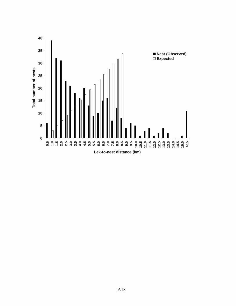
A18

0

5

10

15

20

25

30

35

40

0.5

1.0

1.5

2.0

2.5

3.0

3.5

4.0

4.5

5.0

5.5

6.0

6.5

7.0

7.5

8.0

8.5

9.0

9.5

10.0

10.5

11.0

11.5

12.0

12.5

13.0

13.5

14.0

14.5

15.0

>15

Lek-to-nest distance (km)

Tot

al n

umbe

r of

nes

ts

Nest (Observed)Expected

APPENDIX B

Wyoming Cooperative Fish and Wildlife Research Unit

University of Wyoming, Department 3166

Laramie, WY 82071

Telephone: (307) 766-5415; FAX: (307) 766-5400

Email (corresponding author): [email protected]

RH: Sage-grouse early brooding

GREATER SAGE-GROUSE EARLY BROOD-REARING HABITAT USE

AND PRODUCTIVITY IN WYOMING

Kristin M. Thompson, Corresponding Author, Wyoming Cooperative Fish and Wildlife Research Unit,

University of Wyoming, Laramie, WY 82071.

Matthew J. Holloran, Wyoming Cooperative Fish and Wildlife Research Unit, University of Wyoming,

Laramie, WY 82071.

Steven J. Slater, Wyoming Cooperative Fish and Wildlife Research Unit, University of Wyoming,

Laramie, WY 82071.

Jarren L. Kuipers, Wyoming Cooperative Fish and Wildlife Research Unit, University of Wyoming,

Laramie, WY 82071; Present address: Nebraska Game and Parks Commission, Beatrice, NE

68310.

Stanley H. Anderson, Wyoming Cooperative Fish and Wildlife Research Unit, University of Wyoming,

Laramie, WY 82071.

ABSTRACT.—Populations of greater sage-grouse (Centrocercus urophasianus) have been declining

throughout their range since the 1960s. Productivity, which includes the production and survival of

young, is often cited as a factor in these declines. Greater sage-grouse at three sites in western

Wyoming were radio-equipped and monitored to assess early brood-rearing (i.e, through 14 days post-

B1

hatch) habitat use and productivity. Logistic and linear regression with Akaike’s Information Criterion

were used to evaluate early brood-rearing habitat use and to examine relationships between productivity

and vegetation, insect, and weather parameters. Females with broods were found in areas with greater

sagebrush canopy and grass cover, but lower numbers of invertebrates compared to random areas. The

number of juveniles per female (estimated from wing barrel collections during fall harvest) was

positively associated with the abundance of medium-length Hymenoptera and grass cover, and the

proportion of females with confirmed chicks 14 days post-hatch was positively related to the abundance

of medium-length Coleoptera and total herbaceous cover. Although the specific parameters varied

slightly, greater sage-grouse productivity in Wyoming appeared to be associated with a combination of

insect and herbaceous cover elements. Managing for abundant and diverse insect communities within

dense protective sagebrush stands should help ensure high quality early brood-rearing habitat and

increased greater sage-grouse productivity.

Key words: Greater sage-grouse, early brood-rearing, Centrocercus urophasianus, habitat,

productivity, sagebrush, invertebrate, forb

Over the past 50 years, populations of greater sage-grouse (Centrocercus urophasianus) have

experienced widespread declines (Patterson 1952, Braun 1998, Connelly et al. 2004). Extirpated from

three states and one Canadian province by 1998, the bird is now the focus of conservation and

management concern in much of its remaining range (Connelly et al. 2004). Wyoming remains a

stronghold for greater sage-grouse, where breeding bird numbers were estimated at >20,000 in 1998

(Braun 1998). However, populations throughout the state have also suffered declines; breeding male

numbers decreased by an average of 5.2% annually between 1965 and 2003 (Connelly et al. 2004).

Population declines in tetraonids are often attributed to changes in productivity (Blank et al. 1967,

Bergerud 1988). Productivity (i.e., the production and survival of young) may be affected by a variety

of mainly extrinsic factors, including food availability and weather. Invertebrates are essential in the

first several weeks post-hatch, when chicks require a high-protein diet (Johnson and Boyce 1990).

Insects dominated the diet of one-week old greater sage-grouse chicks in Idaho (Klebenow and Gray

1968), Montana (Peterson 1970), and Colorado (Huwer 2004). Greater sage-grouse broods were

documented using areas with high arthropod abundance in Idaho (Fischer et al. 1996). A study using

captive greater sage-grouse chicks in Wyoming found that all chicks denied insects during the first 10

days post-hatch died, whereas all chicks given insects during this time survived (Johnson and Boyce

1990).

B2

After the first 1 or 2 weeks, forbs begin to gain importance in the diet of chicks. Forbs comprised

75% of the diet of juvenile greater sage-grouse in Montana (Peterson 1970), and were found in 100% of

the crops of two-week-old greater sage-grouse chicks sampled in Idaho (Klebenow and Gray 1968).

Productivity of greater sage-grouse in Oregon was higher in areas where chicks consumed a greater

proportion of forbs and insects (Drut et al. 1994a), and the mass gain of human-imprinted chicks in

Colorado was positively correlated with forb abundance in the diet (Huwer 2004). Forbs may also

provide a food source for chicks by attracting invertebrates (Blenden et al. 1986, Hull et al. 1996,

Jamison et al. 2002). Forb cover, including food forb cover, was higher at sites used by greater sage-

grouse broods compared to non-brood sites in Colorado (Schoenberg 1982), Idaho (Klebenow 1969),

Oregon (Drut et al. 1994b), Washington (Sveum et al. 1998), and Wyoming (Holloran 1999).

Weather may additionally influence productivity during the nesting and brood-rearing periods

(April through August). Cold temperatures may delay nest initiation (Neave and Wright 1969) or stress

incubating females (Smyth and Boag 1984). Spruce grouse (Dendragapus canadensis) incubating in

cold and wet environments produced fewer chicks per hen (Smyth and Boag 1984), whereas

productivity of sharp-tailed grouse (Tympanuchus phasianellus) was positively correlated with May

average temperature (Flanders-Wanner et al. 2004). Newly hatched chicks have poorly developed

thermoregulatory systems (Myhre et al. 1975, Aulie 1976), so they are vulnerable to extreme weather

conditions during the early post-hatch period. A combination of low temperatures, continuous winds,

and precipitation negatively influenced greater sage-grouse brood size during the early hatching period

in Idaho (Dalke et al. 1963). The number of juveniles per adult sharp-tailed grouse harvested was

positively associated with June average temperatures, but negatively correlated with June precipitation

(Flanders-Wanner et al. 2004), and fall harvest numbers of ruffed grouse (Bonasa umbellus) were

positively linked to temperatures in June (Ritcey and Edwards 1963).

Several studies have shown a relationship between brood habitat use and the availability of

invertebrates (Erikstad 1985, Storch 1994, Fischer et al. 1996, Haulton et al. 2003) and forbs

(Klebenow 1969, Peterson 1970, Wallestad 1971, Drut et al. 1994b, Sveum et al. 1998, Holloran 1999).

Other vegetation variables, including sagebrush or shrub canopy cover (Klebenow 1969, Wallestad

1971, Schoenberg 1982, Klott and Lindzey 1990, Holloran 1999), shrub height (Dunn and Braun 1986,

Martin 1970, Sveum et al. 1998, Holloran 1999), and grass or residual grass cover (Sveum et al. 1998,

Holloran 1999) may also act to influence brood habitat use. Literature exists on the importance of

vegetation, invertebrates, and weather to various grouse species. However, research investigating the

influence of these factors on greater sage-grouse early brood-rearing habitat use is lacking, and some of

the factors potentially influencing productivity remain largely speculative. Additionally, most work has

B3

focused on the independent importance of these variables; little has been done to examine their relative

importance, or their interactions. Our objectives were to determine the specific habitat components

associated with greater sage-grouse early brood habitat use and establish which factors were most

strongly related to greater sage-grouse productivity.

STUDY AREA

The research was conducted at three sites in western Wyoming. The 30,400 ha Pinedale study area

(42º45′N, 109º55′W) is located at elevations ranging between 2140 and 2300 m, has a mean

temperature during the nesting/brood-rearing period (April-August) of 10.1º C, and April-August

precipitation averages 14.7 cm. The 45,900 ha Lander site (42º33′N, 108º29′W) is located at elevations

ranging between 1730 and 2470 m. Temperatures during the nesting and brood-rearing periods average

15.7º C, and mean precipitation between April and August is 17.8 cm. The 55,000 ha Kemmerer site

(45º53′N, 110º54′W) is located at elevations ranging between 1900 and 2510 m. Mean temperature

between April and August is 11.4º C, and the average precipitation during this same time is 14 cm

(Western Regional Climate Center, Reno, NV). For detailed description of study areas see Lyon 2000,

Slater 2003, and Kuipers 2004.

All three sites are dominated by sagebrush (Artemisia spp.), mainly Wyoming big sagebrush (A.

tridentata wyomingensis). Other common shrub species include basin big sagebrush (A. t. tridentata),

mountain big sagebrush (A. t. vaseyana), saltbrush (Atriplex spp.), rabbitbrush (Chrysothamnus spp.),

and bitterbrush (Purshia spp.). Wheatgrass (Elymus and Agropyron spp.) and brome (Bromus spp.)

dominate the grass family, while western yarrow (Achillea millefolium), dandelion (Taraxacum

officinale), and lupine (Lupinus spp.) are among the most common forbs (taxonomy Stubbendieck et al.

2003).

METHODS

Data were collected at the Pinedale site between 1999 and 2003, at the Lander site between 2000

and 2003, and at the Kemmerer site between 2000 and 2002, for a total of 12 site-years (e.g., Pinedale

1999, Pinedale 2000, Pinedale 2001, etc.). Female greater sage-grouse were captured at leks in the

early spring of each year using spotlighting and hoop-netting techniques (Giesen et al. 1982, Wakkinen

et al. 1992). Females were fitted with 19.5 or 25.5-g wire-necklace radio-transmitters (Advanced

Telemetry Systems, Inc., Isanti, MN) and tracked with hand-held radio-telemetry receivers and three-

element Yagi antennas. Females were located within the first two weeks of incubation to determine

nest locations, and nest fate (successful or unsuccessful) was determined when the female left the

B4

nesting area. A nest was considered successful if ≥1 egg hatched, determined by presence of detached

eggshell membranes (Girard 1939). Early brood use locations were obtained between 6 and 14 days

post-hatch for females whose nests successfully hatched. For comparison with early brood locations

(i.e., use habitat plots), random habitat locations were obtained by random generation of easting and

northing locations within the study areas.

Vegetation and insect characteristics were measured at both use and random plots. Sagebrush

canopy cover (%) was estimated at each plot using the line-intercept method (Canfield 1941), in which

two perpendicular 30-m transects were centered on each plot. A 1 m-wide belt transect was created

over the 30-m transects to estimate live sagebrush density as the number of plants per square meter

(counted plants included all plants where ≥50% of the plant was within the belt transect). Live

sagebrush height (cm) was estimated as the maximum height, excluding flowering stalks, of each

sagebrush plant encountered during the line-intercept sampling. Ground cover (%) of herbaceous

species (new [i.e., current year’s growth] grasses, residual [i.e., standing dead] grasses, and forbs) was

estimated using the Daubenmire (1959) method: a 20×50-cm open-ended frame was placed over

sampling plots located at 0, 1, and 2.5 m from the center of each transect (12 total frames per plot). We

converted categorical estimates of herbaceous cover to percentages (1 = 2.5%, 2 = 15%, 3 = 37.5%, 4 =

62.5%, 5 = 85%, 6 = 97.5%; Daubenmire 1959) for each of the 12 frames per plot; converted cover

estimates from the 12 frames were averaged to derive a single estimate for each variable per plot.

Herbaceous vegetation variables included total herbaceous cover (all new and residual grasses and

forbs), forb cover (including winterfat [Eurotia lanata] and fringed sagewort [A. frigida]), new grass

cover, and residual grass cover. Ground cover estimates were also calculated for litter and bare ground.

The height of new and residual grasses (cm) was determined by measuring the tallest grasses that

occurred relatively frequently within each Daubenmire frame (heights were meant to be representative

of the herbaceous community; single very tall blades were not included). Height estimates from the 12

Daubenmire frames were averaged to derive single grass height estimates per plot.

Arthropods were sampled using pitfall traps (Greenslade 1964) established along the vegetation

transects at distances of 0, 1, 2.5, 7, and 15 m from the center (17 total pitfall traps per plot). Traps

remained open for 48 hours. Isopropanol was used to kill and preserve trapped insects. Trap contents

were sorted to order, except for arachnids, which were sorted to class. Arthropods were further sorted

into three length categories using guidelines developed from Patterson (1952) and Whitmore et al.

(1986). Arthropods <3 cm were considered small, 3 to 11 cm were considered medium, and those >11

cm were classified as large. Soft-bodied larva, such as grubs and caterpillars, were an exception; the

medium length category contained arthropods between 3 and 15 cm, and only those >15 cm were

B5

considered large. The medium length class was considered the length class of invertebrate most likely

to be selected for and eaten by foraging chicks. Per plot abundances were calculated for each order and

length category of invertebrates.

STATISTICAL ANALYSIS

All site-years with five or fewer use plots were removed because the small sample size did not

allow for accurate representation of the site; this removal left 8 site-years for use in further analyses.

The data for these remaining site-years were winsorized (i.e., outliers in an ordered array were replaced

by their neighboring values; Sokal and Rohlf 1995). Data were winsorized because examination of the

data revealed that single outlying data points (e.g., pitfall traps located on anthills) were unduly

influencing site values in certain instances.

HABITAT USE.—Data were standardized by site (by subtracting the mean and dividing by the

standard deviation; Sokal and Rohlf 1995) to minimize any influence of site on the results. We used

logistic regression to examine habitat use relationships (use vs. random; n = 262). From our original

group of variables, we selected 11 variables to represent three vegetation and insect components.

Variable selection was based on both correlation analyses and published literature (including Klebenow

1969, Dunn and Braun 1986, Klott and Lindzey 1990, Drut et al. 1994b, Fischer et al. 1996, Pyle and

Crawford 1996, and Holloran 1999). Where correlation analyses revealed strong correlations between

variables (e.g., between sagebrush canopy cover, total shrub canopy cover, and litter cover), one

variable from the group was selected based on its importance in the literature. The abundances of

several insect variables, including Orthoptera, were too small to be used in analyses. Sagebrush canopy

cover, live sagebrush density, and sagebrush height represented the shrub component, total forb cover,

total grass (new + residual grass) cover, mean grass (new + residual grass) height, and total herbaceous

cover represented the herbaceous component, and total invertebrate abundance, total Hymenoptera

abundance, medium-length Hymenoptera abundance, and medium-length Coleoptera abundance

represented the insect component. Because this research was primarily exploratory in nature, all

possible two and three variable combinations were used in logistic regression analyses. To reduce

multicollinearity, we did not include variable combinations containing variables correlated by a

Pearson’s correlation coefficient (r) >0.70. Our suite of candidate models included 62 models. Models

were ranked using a small-sample size bias adjusted Akaike’s Information Criterion (AICc; Burnham

and Anderson 2002). Akaike weights (wi) were used to assess the relative importance of each

vegetation and insect variable in distinguishing between use and random sites (Burnham and Anderson

2002). Cumulative Akaike weights were estimated from the entire set of models.

B6

PRODUCTIVITY.—Productivity was measured by two variables: juveniles per female and the

proportion of females with confirmed chicks 14 days post-hatch. Juveniles per female numbers were

obtained from the Wyoming Game and Fish Department and were calculated using juvenile to adult

ratios in wing barrel collections in the fall harvest (Autenrieth et al. 1982, Connelly et al. 2000; data

from Wyoming Game and Fish Department harvest reports, Cheyenne, WY). To ensure that juveniles

per female estimates were comparable to our habitat measurements, we only used harvest estimates

from areas where radio-equipped females were located during the hunting season. The proportion of

females with confirmed chicks was defined as the percentage of successfully nesting females with ≥1

chick alive 14 days post-hatch. The presence of chicks was based on visual confirmation and brooding

females’ reaction to researcher presence (Schroeder et al. 1999). We relocated successfully nesting

females recorded as having no chicks alive 2 to 5 days following the initial location to confirm brood

loss. Vegetation, insect, and weather variables were again selected based on correlation analyses and

their importance in the literature (including Dalke et al. 1963, Klebenow and Gray 1968, Peterson 1970,

and Drut et al. 1994a). Vegetation parameters included total forb cover, total grass cover, mean grass

height, and total herbaceous cover; the insect component was comprised of total invertebrate

abundance, total Hymenoptera abundance, medium-length Hymenoptera abundance, and medium-

length Coleoptera abundance. We used one-way analysis of variance (ANOVA) to examine the effect

of site and year on the variables; those variables that differed significantly by site or year (P ≤0.1) were

standardized by site (Sokal and Rohlf 1995).

Weather data were obtained from the Western Regional Climate Center (Western Regional Climate

Center, Reno, NV). Where data were unavailable, we extrapolated (using kriging techniques in a GIS;

Burrough and McDonnell 1998) using data from nearby weather stations. To minimize any effects of

site, both temperature and precipitation variables were calculated as a percent of average (period of

record 1948 – 2004). It seemed likely that the interaction of temperature and precipitation could have a

greater effect on productivity than either variable alone, so we created a combination

temperature/precipitation (TempPre) variable, calculated by dividing temperature by precipitation.

Therefore, a hot and dry month would have a high TempPre value, whereas a wet and cold month

would have a low TempPre value. The TempPre variable was developed for April – May

(AprMay_TempPre), June (Jun_TempPre), and July – August (JulAug_TempPre). Because estimates

of the proportion of females with confirmed chicks were generated by mid-June, JulAug_TempPre was

included only in the juveniles per female analysis.

We generated a suite of models using our selected vegetation, insect, and weather variables. To

avoid over-parameterizing the models (Hosmer and Lemeshow 1989), variable combinations were

B7

limited to 2 variables. All possible 2-variable combinations (except those in which the variables were

correlated to each other by r >0.70) were included in the multiple regression analysis, with either

juveniles per female or the proportion of females with confirmed chicks as the dependent variable. Our

suite of candidate models included 39 models for use in the juveniles per female analysis and 32 models

for the proportion of females with confirmed chicks analysis. Mean site-year data (n = 8 site-years)

were used for all productivity analyses. Akaike’s Information Criterion with a small-sample bias

adjustment (AICc) was used to select the most parsimonious model(s), and Akaike weights (wi) were

used to determine the relative importance of the habitat and insect components (Burnham and Anderson

2002). Cumulative variable weights were estimated from the entire set of models. Productivity

analyses were conducted using mean site-year data obtained from random plots (vs. use plots). The

weather variables and the juveniles per female numbers used in our analyses were site-level data, and

we believed that data collected from random plots were more representative of annual site conditions.

All spatial analyses were conducted using ArcView GIS v3.2 (ESRI, Inc. 1998), and statistical

analyses were conducted using Minitab Release 13 (Minitab, Inc. 1994) and SAS v8.2 (SAS Institute,

Inc. 1990).

RESULTS

Data used in habitat use analyses (i.e., site-years with more than 5 use plots) included Pinedale 1999

(n = 9 use plots [i.e., locations for 9 different females with broods], 9 random plots), 2000 (n = 8 use, 8

random), 2002 (n = 16 use, 22 random), and 2003 (n = 15 use, 24 random); Lander 2001 (n = 7 use, 29

random), 2002 (n = 9 use, 19 random), and 2003 (n = 10 use, 39 random); and Kemmerer 2002 (n = 8

use, 30 random). Productivity analyses were conducted using mean data from these years (n = 8 site-

years). Hymenoptera were the most common arthropods sampled, making up nearly 60% of the total

arthropod abundance in both use and random habitats. Coleoptera were also fairly common,

comprising just over 20% of the total arthropod abundance. Most Hymenoptera (73%) and Coleoptera

(62%) collected were adults, and were within the medium-length category. The majority of the shrub

cover was comprised of sagebrush; mean sagebrush canopy cover from use and random locations

combined was 20.0% (±sx̄; ±0.7). Mean live sagebrush density was 1.7 (±0.1) plants/m2; mean

sagebrush height was 27.2 (±0.6) cm. Total herbaceous cover averaged 26.2% (±1.1); total forb cover

and total grass cover averaged 4.9% (±0.4) and 9.0% (±0.3), respectively. Mean grass + residual grass

height was 10.7 (±0.2) cm.

HABITAT USE.—Fourteen of our 62 models had AICc values within 2 units of the minimum AICc

value (Table 1), suggesting substantial support (Burnham and Anderson 2002). Thirteen of the 14

B8

models statistically fit the data (Hosmer-Lemeshow goodness-of-fit test statistics). In accordance with

AIC principles (Burnham and Anderson 2002) all models were retained in the analysis (post hoc

examination of the data after removing models that did not statistically fit the data [Hosmer and

Lemeshow 1989] indicated that conclusions did not differ from the original analysis: cumulative

Akaike weights indicating relative variable importance were virtually unaffected). Based on AICc

weights, the top model was only marginally better in predicting habitat use than were the other 13

candidate models (i.e., evidence ratios ≤2.7; Burnham and Anderson 2002). However, although none

of the models was clearly the best, the cumulative Akaike weight was fairly substantial for the

sagebrush cover variable (0.71), indicating that it may be a good predictor of habitat use. Examination

of regression data directional trends suggested that broods were using areas with increased sagebrush

canopy cover and density, total grass cover, and mean grass height, and decreased invertebrate

abundance compared to random areas (Table 1). Forb abundance was slightly positive, but appeared in

only one of the top 14 models.

PRODUCTIVITY.—Two models in the juveniles per female analysis fell within 2 units of the

minimum AICc value (Burnham and Anderson 2002). The top model contained the terms medium-

length Hymenoptera abundance and total grass cover, and had an AICc weight of 0.46. The second-

ranked model included the variables medium-length Hymenoptera abundance and medium-length

Coleoptera abundance (AICc weight 0.17). The number of juveniles per female was positively

associated with each of the independent variables in these top models. Based on cumulative AICc

weights, the most important parameters influencing juveniles per female appeared to be medium-length

Hymenoptera abundance and total grass cover (Table 2).

The analysis of the proportion of females with confirmed chicks 14 days post-hatch yielded one

highly plausible model, which contained the variables total herbaceous cover and medium-length

Coleoptera abundance. The AICc weight associated with this model was 0.98 and the evidence ratio

was 57.3, suggesting that, given the data, this model was likely to be the best model (Burnham and

Anderson 2002). The proportion of females with confirmed chicks was positively associated with both

total herbaceous cover and medium-length Coleoptera abundance. Total herbaceous cover and

medium-length Coleoptera abundance were also the most important individual parameters, based on

cumulative AICc weights (Table 2).

DISCUSSION

Greater sage-grouse broods in Wyoming used habitats with greater sagebrush and grass cover, but

fewer insects compared to random sites. The abundance of forbs did not appear to play a large role in

B9

early brood habitat use. Though numerous researchers have examined habitat use by broods, results are

somewhat inconsistent. Similar to the results of our study, greater sage-grouse in Colorado used areas

with greater sagebrush canopy cover than random sites (Dunn and Braun 1986); however, that study

included not only females with broods, but juveniles and unsuccessfully nesting females. Schoenberg

(1982) found no significant difference in sagebrush cover between brood use sites and random sites,

whereas Klebenow (1969), Klott and Lindzey (1990), and Holloran (1999) documented brood use of

sites with lower sagebrush or shrub cover than random sites. Greater sage-grouse broods in Idaho used

areas with greater abundance of Hymenoptera than non-brood locations (Fischer et al. 1996).

Numerous studies of other galliform species have found similar results: capercaillie (Tetrao urogallus),

black grouse (Tetrao tetrix), lesser prairie-chicken (Tympanuchus pallidicinctus), and ruffed grouse

broods have been documented selecting areas with greater invertebrate abundances than available areas

(Storch 1994, Baines et al. 1996, Jamison et al. 2002, Haulton et al. 2003). In contrast, our broods were

found in areas with lower amounts invertebrates than were generally available.

One potential reason for discrepancies between our results and those from other studies is that

investigator presence had an effect on habitat use. Although we made every attempt to avoid

disturbance to birds while radio-tracking, it is possible that once broods heard or sighted investigators,

the birds changed their focus from foraging to escape. This could have biased our results toward

security cover (i.e., increased sagebrush cover) and away from foraging habitat (i.e., increased

arthropods and forbs). Greater sage-grouse are often found near habitat edges (Dunn and Braun 1986),

so even small-scale movements of 5 to 10 m may have been enough to shift birds between different

habitat types. Although we do not believe that we influenced brood habitat use, if broods did move

during the tracking process it would suggest that they were feeding in areas closely associated with

suitable security cover.

We believe a more likely explanation is based on temporal differences between studies. Our study

examined brood habitat use early in the brood-rearing period (before chicks were two weeks old).

Holloran (1999) collected data on chicks between 2 and 4 weeks of age, Klebenow (1969) examined

habitat use by broods up to 7 weeks of age, and Klott and Lindzey (1990) obtained brood locations

throughout the summer. Grouse chicks experience heavy losses within the first few weeks of life.

Survival of greater sage-grouse chicks to 21 days old in Idaho ranged from 21 to 50% (Burkepile et al.

2002), and between 14 and 33% of chicks survived to 50 days of age in Washington and Canada

(Schroeder 1997, Aldridge and Brigham 2001). Crawford et al. (2004) averaged the results of 3 studies

to come up with an estimated 10% survival rate from hatch to the first potential breeding season. These

studies did not examine how much mortality occurred during the first 14 days; however, Holloran

B10

(1999) documented the majority of chick loss during the first 2 to 3 weeks. Patterson (1952) suggested

that although a myriad of factors may be involved, losses to predation potentially account for the

greatest amount of juvenile mortality in greater sage-grouse. In addition, several authors suggest that

predation may be one factor limiting annual tetraonid productivity (Batterson and Morse 1948,

Marcström et al. 1988, Baines 1991).

Greater sage-grouse broods in Wyoming appeared to be selecting habitats with increased security

cover during the first two weeks post-hatch. Chicks are generally not capable of flight before 10 days

to two weeks of age (Girard 1937, Wallestad 1975), thus the presence of dense protective cover may be

even more important for females with younger broods than for older broods that have alternate means

of escape. The need for foraging areas in close proximity to protective cover has been well documented

(Klebenow 1969, Wallestad 1971, Klott and Lindzey 1990, Sveum et al. 1998, Holloran 1999). Insect

abundances were negatively correlated with sagebrush cover (r = -0.15 total arthropods; -0.12 optimal-

length Hymenoptera; -0.11 total Hymenoptera), thus lower levels of this component in brood use areas

in Wyoming were likely an artifact of these correlations and not selection.

Forb cover did not appear to be a driving factor in early brood habitat use. Although many studies

have documented brood use of sites with high forb abundance (Klebenow 1969, Klott and Lindzey

1990, Sveum et al. 1998, Holloran 1999), these studies examined habitat use later in the brood-rearing

period. Because we estimated early brood habitat use to 14 days post-hatch, forbs may not yet have

been the main component of the diet. Patterson (1952) suggests that vegetation begins to gain

importance in chick diets after the first few weeks of life. Klebenow and Gray (1968), Peterson (1969)

and Huwer (2004) found that invertebrates dominated the diet of greater sage-grouse chicks during the

first week, before forbs began to gain importance as a food source.

The ratio of juveniles to adult females in the fall harvest appeared to be most strongly influenced by

invertebrate abundance and grass cover. Our top two models both included medium-length

Hymenoptera abundance. Hymenoptera, which in our study consisted mainly of ants (Formicidae),

have been shown to be an important food item for young chicks; ants were found in 75% of the crops of

birds 1 to 4 weeks old in Montana (Peterson 1970) and in up to 100% of the crops of juvenile greater

sage-grouse collected in Idaho (Klebenow and Gray 1968). Johnson and Boyce (1990) found that

insects were crucial for survival of young sage grouse chicks, and studies of several other galliform

species have found that invertebrate abundance was positively associated with productivity (Green

1984, Hill 1985, Park et al. 2001). Total grass cover was the top vegetation variable; nearly 60% of the

AICc weight was attributed to models that included this variable. It likely served a protective function

by screening foraging broods from potential predators.

B11

The factors associated with the proportion of females with confirmed chicks appeared to be well

defined. AIC analysis yielded only one highly plausible model containing the variables medium-length

Coleoptera abundance and total herbaceous cover. Like Hymenoptera, Coleoptera are often a principal

component in juvenile greater sage-grouse diets (Klebenow and Gray 1968, Peterson 1970). Total

herbaceous cover was comprised of both grasses and forbs. Therefore, it may have served a dual

function of providing both protection and food sources. Total forb cover was positively correlated with

both medium-length Hymenoptera (r = 0.68) and medium-length Coleoptera (r = 0.81) abundances.

Whereas forb cover did appear in a second-tier model (i.e., ΔAICc between 2 and 4) in the juveniles per

female analysis, it was not strongly related to the proportion of females with confirmed chicks. Again,

because we examined this measure of productivity by 14 days post-hatch, forbs may not yet have been

the major component of the diet.

We found virtually no relationship between weather and productivity. It is possible that short-lived,

extreme weather conditions (e.g., heavy rainfall, severe cold spell) influenced productivity, but these

occurrences were not detectable using annual weather data. However, the trends we did see were

consistent; all weather variables were positively associated with our two measures of productivity.

Warm and dry conditions appeared to be more favorable for productivity than cold and wet conditions.

Our study suggests that abundant medium-length insects within heavy sagebrush cover will be most

beneficial to juvenile greater sage-grouse. During the early brood-rearing period, broods used sites

within or near dense (average 20% canopy cover) sagebrush cover, and increased productivity was

positively associated with abundance of insects and herbaceous cover. Although managing directly for

invertebrates is likely not feasible, it may be possible to indirectly manage for insect abundance through

the manipulation of vegetation. Invertebrate biomass has been found to be positively correlated to forb

abundance (Southwood and Cross 1969, Blenden et al. 1986, Hull et al. 1996, Jamison et al. 2002);

thus, enhancement of the forb component could serve a dual function by directly providing a food

resource while ensuring the availability of insects. Development and maintenance of a productive forb

layer should not come at the expense of sagebrush cover, however. The overriding factor affecting

habitat use by greater sage-grouse broods appeared to be the presence of protective sagebrush cover;

therefore, this cover should be maintained while increasing the understory herbaceous layer. Managing

for a productive, diverse understory within dense sagebrush stands should help ensure high quality early

brood-rearing habitat, and enhance the potential for increased greater sage-grouse productivity.

B12

ACKNOWLEDGMENTS

Funding was provided by the Wyoming Game and Fish Department, Bureau of Land Management,

Department of Energy, 3-Shot Sage-grouse Foundation, Yellowstone-to-Yukon Initiative, EnCana Oil

and Gas, and the Animal Damage Management Board. We thank D.R. Edmunds, R.A. Holloran, B.K.

Holtby, M.A. Kaemingk, A.G. Lyon, Mr. and Mrs. T.W. Malmberg, C.M. Sazama, C.G. Taber, Mr. and

Mrs. N.A. Tratnik, and G.L. Wilson for assistance with field research. France Flying Service (Rawlins,

WY) and Mountain Air Research (Driggs, ID) provided logistical support. We thank A.D. Apa, A.J.

Carlson, J.W. Connelly, W.A. Hubert, D.D. Paulson, S.E. Richman, and an anonymous reviewer for

valuable comments on earlier versions of this manuscript.

LITERATURE CITED

ALDRIDGE, C.L. AND R.M. BRIGHAM. 2001. Nesting and reproductive activities of greater sage-grouse


AULIE, A. 1976. The pectoral muscles and the development of thermoregulation in chicks of willow

ptarmigan (Lagopus lagopus). Comparative Biochemistry and Physiology 53A:343-346.

AUTENRIETH, R., M. MOLINI, AND C. BRAUN. 1982. Sage grouse management practices. Western

States Sage Grouse Committee, Technical Bulletin 1. Twin Falls, Idaho. 42 pp.

BAINES, D. 1991. Factors contributing to local and regional variation in black grouse breeding success

in northern Britain. Ornis Scandinavica 22:264-269.

——, I.A. WILSON, AND G. BEELEY. 1996. Timing of breeding in Black Grouse Tetrao tetrix and

Capercaillie Tetrao urogallus and distribution of insect food for the chicks. Ibis 138:181-187.

BATTERSON, W.M. AND W.B. MORSE. 1948. Oregon sage grouse. Oregon Fauna Serv. 1. Oregon

Game Commission, Portland. 29 pp.

BERGERUD, A.T. 1988. Population ecology of North American grouse. Pages 578-685 in A.T.

Bergerud and M.W. Gratson, editors, Adaptive strategies and population ecology of northern

grouse. University of Minnesota Press, Minneapolis.

BLANK, T.H., T.R.E. SOUTHWOOD, AND D.J. CROSS. 1967. The ecology of the partridge. I. Outline of

population processes with particular reference to chick mortality and nest density. Journal of

Animal Ecology 36:549-556.

BLENDEN, M.D., M.J. ARMBRUSTER, T.S. BASKETT, AND A.H. FARMER. 1986. Evaluation of model

assumptions: the relationship between plant biomass and arthropod abundance. Pages 11-14 in J.

Verner, M.L. Morrison, and C.J. Ralph, editors, Modeling habitat relationships of terrestrial

vertebrates. University of Wisconsin Press, Madison.

B13

BRAUN, C.E. 1998. Sage grouse declines in western North America: what are the problems? Pages

139-156 in Proceedings of the 1998 Western Association of State Fish and Wildlife Agencies,

Jackson, WY.

BURKEPILE, N.A., J.W. CONNELLY, D.W. STANLEY, AND K.P. REESE. 2002. Attachment of

radiotransmitters to one-day-old sage grouse chicks. Wildlife Society Bulletin 30:93-96.

BURNHAM, K.P. AND D.R. ANDERSON. 2002. Model selection and multimodel inference: a practical

information-theoretic approach. 2nd edition. Springer-Verlag, New York, NY. 488 pp.

BURROUGH, P.A. AND R.A. MCDONNELL. 1998. Principles of geographical information systems.

Oxford University Press, New York, NY. 333 pp.

CANFIELD, R. 1941. Application of the line intercept method in sampling of range vegetation. Journal

of Forestry 39:386-394.

CONNELLY, J. W., M.A. SCHROEDER, A.R. SANDS, AND C.E. BRAUN. 2000. Guidelines to manage sage


——, S.T. KNICK, M.A. SCHROEDER, AND S.J. STIVER. 2004. Conservation assessment of greater sage-

grouse and sagebrush habitats. Western Association of Fish and Wildlife Agencies. Unpublished

Report. Cheyenne, WY. 601 pp.

CRAWFORD, J.A., R.A. OLSON, N.E. WEST, J.C. MOSLEY, M.A. SCHROEDER, T.D. WHITSON, R.F.

MILLER, M.A. GREGG, AND C.S. BOYD. 2004. Ecology and management of sage-grouse and sage-

grouse habitat. Journal of Range Management 57:2-19.

DALKE, P.D., D.B. PYRAH, D.C. STANTON, J.E. CRAWFORD, AND E.F. SCHLATTERER. 1963. Ecology,

productivity, and management of sage grouse in Idaho. Journal of Wildlife Management 27:811-

841.

DAUBENMIRE, R.F. 1959. A canopy-coverage method of vegetational analysis. Northwest Science

33:43-64.

DRUT, M.S., W.H. PYLE, AND J.A. CRAWFORD. 1994a. Technical note: diets and food selection of sage

grouse chicks in Oregon. Journal of Range Management 47:90-93.

——, J.A. CRAWFORD, AND M.A. GREGG. 1994b. Brood habitat use by sage grouse in Oregon. Great

Basin Naturalist 54:170-176.

DUNN, P.O. AND C.E. BRAUN. 1986. Summer habitat use by adult female and juvenile sage grouse.


ERIKSTAD, K.E. 1985. Growth and survival of willow grouse chicks in relation to home range size,

brood movements and habitat selection. Ornis Scandinavica 16:181-190.

B14

ESRI, INC. 1998. Introduction to ArcView® GIS. Environmental Systems Research Institute, Inc.,

Redlands, CA. 604 pp.

FISCHER, R.A., K.P. REESE, AND J.W. CONNELLY. 1996. An investigation of fire effects within xeric

sage grouse brood habitat. Journal of Range Management 49:194-198.

FLANDERS-WANNER, B.L., G.C. WHITE, AND L.L. MCDANIEL. 2004. Weather and prairie grouse:

dealing with effects beyond our control. Wildlife Society Bulletin 32:22-34.

GIESEN, K.M., T.J. SCHOENBERG, AND C.E. BRAUN. 1982. Methods for trapping sage grouse in


GIRARD, G.L. 1937. Life history, habits and food of the sage grouse, Centrocercus urophasianus

Bonaparte. University of Wyoming Publications, Publication 3. University of Wyoming, Laramie.

56 pp.

——. 1939. Notes on life history of the shoveler. Transactions of the North American Wildlife

Conference 4:364-371.

GREEN, R.E. 1984. The feeding ecology and survival of partridge chicks (Alectoris rufa and Perdix

perdix) on arable farmland in East Anglia. Journal of Applied Ecology 21:817-830.

GREENSLADE, P.J.M. 1964. Pitfall trapping as a method for studying populations of Carabidae

(Coleoptera). Journal of Animal Ecology 33:301-310.

HAULTON, G.S., D.F. STAUFFER, R.L. KIRKPATRICK, AND G.W. NORMAN. 2003. Ruffed grouse

(Bonasa umbellus) brood microhabitat selection in the southern Appalachians. American Midland

Naturalist 150:95-103.

HILL, D.A. 1985. The feeding ecology and survival of pheasant chicks on arable farmland. Journal of

Applied Ecology 22:645-654.

HOLLORAN, M.J. 1999. Sage grouse (Centrocercus urophasianus) seasonal habitat use near Casper,

Wyoming. Master’s thesis, University of Wyoming, Laramie.

HOSMER, D.W. AND S. LEMESHOW. 1989. Applied logistic regression. John Wiley & Sons, New York,

NY. 307 pp.

HULL, S.D., R.J. ROBEL, AND K.E. KEMP. 1996. Summer avian abundance, invertebrate biomass, and

forbs in Kansas CRP. Prairie Naturalist 28:1-12.

HUWER, S.L. 2004. Evaluating greater sage-grouse brood habitat using human-imprinted chicks.

Master’s thesis, Colorado State University, Fort Collins.

JAMISON, B.E., R.J. ROBEL, J.S. PONTIUS, AND R.D. APPLEGATE. 2002. Invertebrate biomass:

associations with lesser prairie-chicken habitat use and sand sagebrush density in southwestern

Kansas. Wildlife Society Bulletin 30:517-526.

B15

JOHNSON, G.D. AND M.S. BOYCE. 1990. Feeding trials with insects in the diet of sage grouse chicks.


KLEBENOW, D.A. 1969. Sage grouse nesting and brood habitat in Idaho. Journal of Wildlife


—— AND G.M. GRAY. 1968. Food habits of juvenile sage grouse. Journal of Range Management

21:80-83.

KLOTT, J.H. AND F.G. LINDZEY. 1990. Brood habitats of sympatric sage grouse and Columbian sharp-

tailed grouse in Wyoming. Journal of Wildlife Management 54:84-88.

KUIPERS, J.L. 2004. Grazing system and linear corridor influences on greater sage-grouse

(Centrocercus urophasianus) habitat selection and productivity. Master’s thesis, University of

Wyoming, Laramie.

LYON, A.G. 2000. The potential effects of natural gas development on sage grouse near Pinedale,

Wyoming. Master’s thesis, University of Wyoming, Laramie.

MARCSTRÖM, V., R.E. KENWARD, AND E. ENGREN. 1988. The impact of predation on boreal tetraonids

during vole cycles: an experimental study. Journal of Animal Ecology 57:859-872.

MARTIN, N.S. 1970. Sagebrush control related to habitat and sage grouse occurrence. Journal of


MINITAB, INC. 1994. Minitab® User’s Guide, Release 10 for Windows. State College, PA.

268 pp.

MYHRE, K., M. CABANAC AND G. MYHRE. 1975. Thermoregulatory behavior and body temperature in

chicks of willow grouse (Lagopus lagopus lagopus). Poultry Science 54:1174-1179.

NEAVE, D.J. AND B.S. WRIGHT. 1969. The effects of weather and DDT spraying on a ruffed grouse

population. Journal of Wildlife Management 33:1015-1020.

PARK, K.J., P.A. ROBERTSON, S.T. CAMPBELL, R. FOSTER, Z.M. RUSSELL, D. NEWBORN, AND P.J.

HUDSON. 2001. The role of invertebrates in the diet, growth and survival of red grouse (Lagopus

lagopus scoticus) chicks. Journal of Zoology, London 254:137-145.

PATTERSON, R.L. 1952. The sage grouse in Wyoming. Wyoming Game and Fish Commission. Sage

Books, Inc., Denver, CO. 341 pp.

PETERSON, J.G. 1970. The food habitats and summer distribution of juvenile sage grouse in central


PYLE, W.H. AND J.A. CRAWFORD. 1996. Availability of foods of sage grouse chicks following

prescribed fire in sagebrush-bitterbrush. Journal of Range Management 49:320-324.

B16

RITCEY, R.W. AND R.Y. EDWARDS. 1963. Grouse abundance and June temperatures in Wells Gray

Park, British Columbia. Journal of Wildlife Management 27:604-606.

SAS INSTITUTE, INC. 1990. SAS/STAT® User’s Guide, Version 6. 4th edition. Volume 2. SAS

Institute, Cary, NC. 846 pp.

SCHOENBERG, T.J. 1982. Sage grouse movements and habitat selection in North Park, Colorado.

Master’s thesis, Colorado State University, Fort Collins.

SCHROEDER, M.A. 1997. Unusually high reproductive effort by sage grouse in a fragmented habitat in


——, J.R. YOUNG, and C.E. BRAUN. 1999. Sage grouse (Centrocercus urophasianus). Pages 1-28 in

A. Poole and F. Gill, editors, The Birds of North America, No. 425. The Birds of North

America, Inc., Philadelphia, PA.

SLATER, S.J. 2003. Sage grouse (Centrocercus urophasianus) use of different-aged burns and the

effects of coyote control in southwestern Wyoming. Master’s thesis, University of Wyoming,

Laramie.

SMYTH, K.E. AND D.A. BOAG. 1984. Production in spruce grouse and its relationship to environmental

factors and population parameters. Canadian Journal of Zoology 62:2250-2257.

SOKAL, R.R. AND F.J. ROHLF. 1995. Biometry. 3rd edition. W. H. Freeman, New York, NY. 887 pp.

SOUTHWOOD, T.R.E. AND D.J. CROSS. 1969. The ecology of the partridge. III. Breeding success and

the abundance of insects in natural habitats. Journal of Animal Ecology 38:497-509.

STORCH, I. 1994. Habitat and survival of capercaillie Tetrao urogallus nests and broods in the

Bavarian Alps. Biological Conservation 70:237-243.

STUBBENDIECK, J., S.L. HATCH, AND L.M. LANDHOLT. 2003. North American wildland plants: a field

guide. 6th edition. University of Nebraska Press, Lincoln. 501 pp.

SVEUM, C.M., J.A. CRAWFORD, AND W.D. EDGE. 1998. Use and selection of brood-rearing habitat by

sage grouse in south central Washington. Great Basin Naturalist 58:344-351.

WAKKINEN, W.L., K.P. REESE, J.W. CONNELLY, AND R.A. FISCHER. 1992. An improved spotlighting


WALLESTAD, R.O. 1971. Summer movements and habitat use by sage grouse broods in central


——. 1975. Life history and habitat requirements of the sage grouse in central Montana. Division of

Wildlife, Montana Department of Game and Fish. 65 pp.

WHITMORE, R.W., K.P. PRUESS, AND R.E. GOLD. 1986. Insect food selection by 2-week-old ring-

necked pheasant chicks. Journal of Wildlife Management 50:223-228.

B17

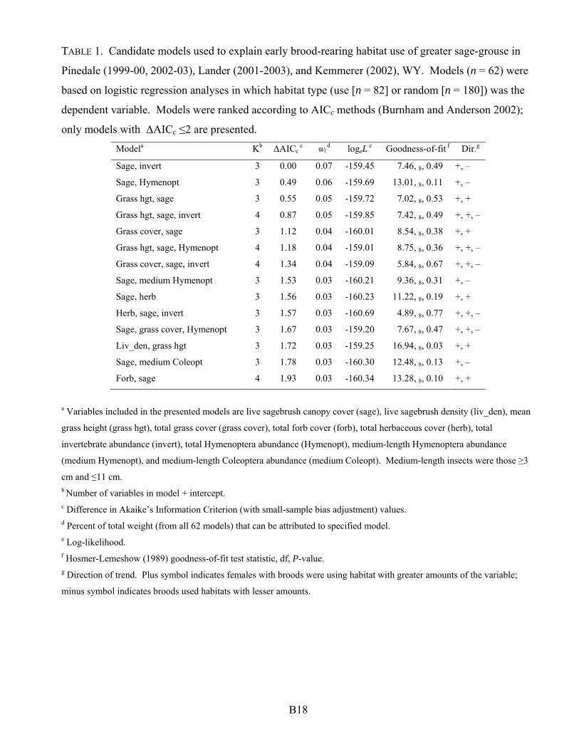
TABLE 1. Candidate models used to explain early brood-rearing habitat use of greater sage-grouse in

Pinedale (1999-00, 2002-03), Lander (2001-2003), and Kemmerer (2002), WY. Models (n = 62) were

based on logistic regression analyses in which habitat type (use [n = 82] or random [n = 180]) was the

dependent variable. Models were ranked according to AICc methods (Burnham and Anderson 2002);

only models with ΔAICc ≤2 are presented.

Modela Kb ΔAICc c wi d logeL e Goodness-of-fit f Dir.g

Sage, invert 3 0.00 0.07 -159.45 07.46, 8, 0.49 +, –

Sage, Hymenopt 3 0.49 0.06 -159.69 13.01, 8, 0.11 +, –

Grass hgt, sage 3 0.55 0.05 -159.72 07.02, 8, 0.53 +, +

Grass hgt, sage, invert 4 0.87 0.05 -159.85 07.42, 8, 0.49 +, +, –

Grass cover, sage 3 1.12 0.04 -160.01 08.54, 8, 0.38 +, +

Grass hgt, sage, Hymenopt 4 1.18 0.04 -159.01 08.75, 8, 0.36 +, +, –

Grass cover, sage, invert 4 1.34 0.04 -159.09 05.84, 8, 0.67 +, +, –

Sage, medium Hymenopt 3 1.53 0.03 -160.21 09.36, 8, 0.31 +, –

Sage, herb 3 1.56 0.03 -160.23 11.22, 8, 0.19 +, +

Herb, sage, invert 3 1.57 0.03 -160.69 04.89, 8, 0.77 +, +, –

Sage, grass cover, Hymenopt 3 1.67 0.03 -159.20 07.67, 8, 0.47 +, +, –

Liv_den, grass hgt 3 1.72 0.03 -159.25 16.94, 8, 0.03 +, +

Sage, medium Coleopt 3 1.78 0.03 -160.30 12.48, 8, 0.13 +, –

Forb, sage 4 1.93 0.03 -160.34 13.28, 8, 0.10 +, +

a Variables included in the presented models are live sagebrush canopy cover (sage), live sagebrush density (liv_den), mean

grass height (grass hgt), total grass cover (grass cover), total forb cover (forb), total herbaceous cover (herb), total

invertebrate abundance (invert), total Hymenoptera abundance (Hymenopt), medium-length Hymenoptera abundance

(medium Hymenopt), and medium-length Coleoptera abundance (medium Coleopt). Medium-length insects were those ≥3

cm and ≤11 cm.

b Number of variables in model + intercept. c Difference in Akaike’s Information Criterion (with small-sample bias adjustment) values. d Percent of total weight (from all 62 models) that can be attributed to specified model. e Log-likelihood.

f Hosmer-Lemeshow (1989) goodness-of-fit test statistic, df, P-value. g Direction of trend. Plus symbol indicates females with broods were using habitat with greater amounts of the variable;

minus symbol indicates broods used habitats with lesser amounts.

B18

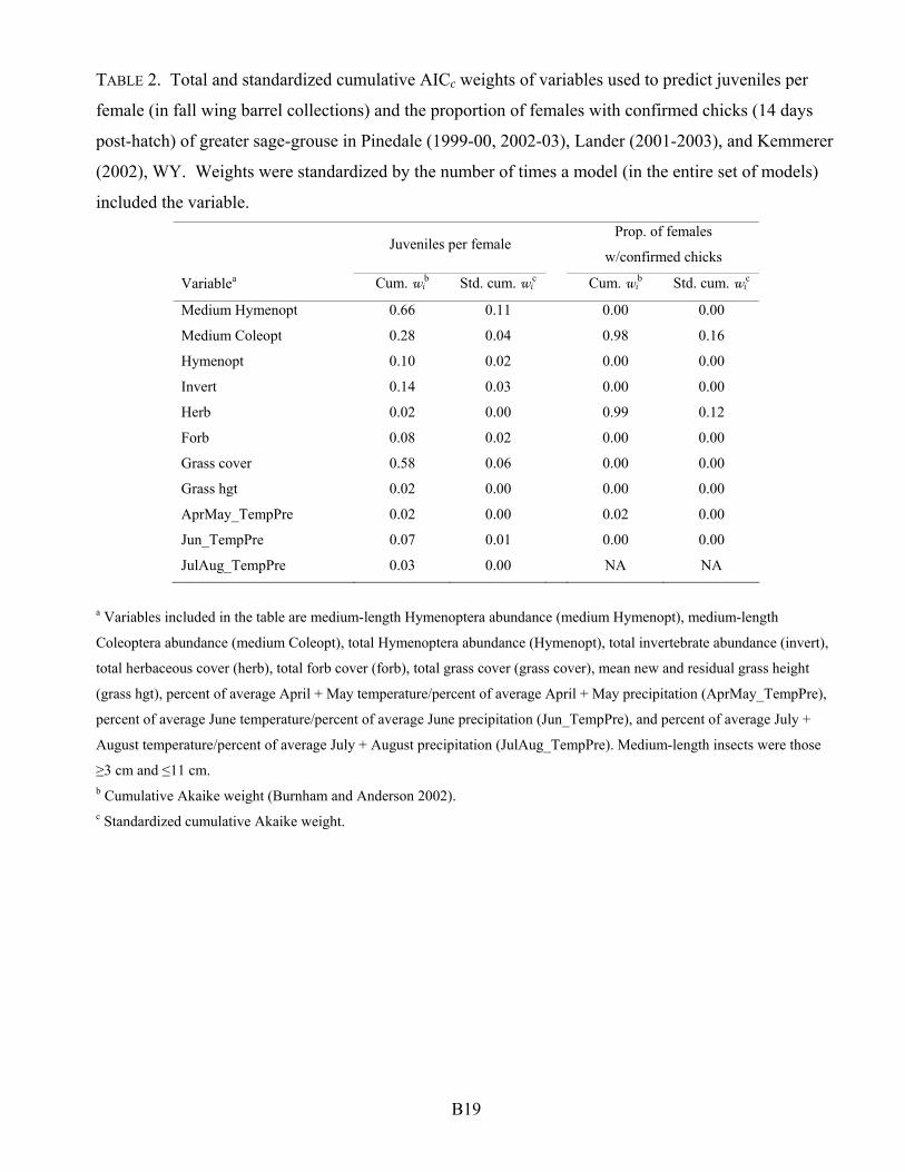
TABLE 2. Total and standardized cumulative AICc weights of variables used to predict juveniles per

female (in fall wing barrel collections) and the proportion of females with confirmed chicks (14 days

post-hatch) of greater sage-grouse in Pinedale (1999-00, 2002-03), Lander (2001-2003), and Kemmerer

(2002), WY. Weights were standardized by the number of times a model (in the entire set of models)

included the variable.

Juveniles per female Prop. of females

w/confirmed chicks

Variablea Cum. wib Std. cum. wic Cum. wib Std. cum. wic

Medium Hymenopt 0.66 0.11 0.00 0.00

Medium Coleopt 0.28 0.04 0.98 0.16

Hymenopt 0.10 0.02 0.00 0.00

Invert 0.14 0.03 0.00 0.00

Herb 0.02 0.00 0.99 0.12

Forb 0.08 0.02 0.00 0.00

Grass cover 0.58 0.06 0.00 0.00

Grass hgt 0.02 0.00 0.00 0.00

AprMay_TempPre 0.02 0.00 0.02 0.00

Jun_TempPre 0.07 0.01 0.00 0.00

JulAug_TempPre 0.03 0.00 NA NA

a Variables included in the table are medium-length Hymenoptera abundance (medium Hymenopt), medium-length

Coleoptera abundance (medium Coleopt), total Hymenoptera abundance (Hymenopt), total invertebrate abundance (invert),

total herbaceous cover (herb), total forb cover (forb), total grass cover (grass cover), mean new and residual grass height

(grass hgt), percent of average April + May temperature/percent of average April + May precipitation (AprMay_TempPre),

percent of average June temperature/percent of average June precipitation (Jun_TempPre), and percent of average July +

August temperature/percent of average July + August precipitation (JulAug_TempPre). Medium-length insects were those

≥3 cm and ≤11 cm. b Cumulative Akaike weight (Burnham and Anderson 2002). c Standardized cumulative Akaike weight.

B19

APPENDIX C

GREATER SAGE-GROUSE RESEARCH IN WYOMING: AN OVERVIEW OF STUDIES

CONDUCTED BY THE WYOMING COOPERATIVE FISH AND WILDLIFE RESEARCH UNIT

BETWEEN 1994 AND 2005

Matthew J. Holloran, Wyoming Cooperative Fish and Wildlife Research Unit, University of Wyoming,

Box 3166 University Station, Laramie, WY, 82071, USA.

[email protected]; 307 766 5415 (voice); 307 766 5400 (fax).

Stanley H. Anderson, Wyoming Cooperative Fish and Wildlife Research Unit, University of Wyoming,

Box 3166 University Station, Laramie, WY, 82071, USA.

ABSTRACT

Greater sage-grouse (Centrocercus urophasianus) populations have been declining throughout

Wyoming since the 1960s. Game and land managers, sportsmen organizations, and Wyoming citizens

have been concerned over the plight of the sage-grouse for over a half-century, but this concern has

escalated within the last decade. In 1994, the first of a series of 10 research projects on greater sage-

grouse in Wyoming was initiated; the Wyoming Cooperative Research Unit was responsible for

conducting these studies. The projects have focused on a wide array of objectives, including greater

sage-grouse microsite and landscape scale seasonal habitat use and the identification of limiting

seasonal habitats, the effects of mineral extraction activity on greater sage-grouse populations, greater

sage-grouse seasonal use of habitats manipulated by fire, livestock grazing management system

influences on greater sage-grouse productivity, and the response of greater sage-grouse populations to

predator control programs. This report is a synopsis of the results from the research conducted by the

Wyoming Cooperative Research Unit on greater sage-grouse since 1994. Detailed information

pertaining to methods and site-specific results are found in the original job completion reports

(Wyoming Game and Fish Department, Cheyenne, WY, USA) and theses (University of Wyoming,

Laramie, WY, USA).

C1

ACKNOWLEDGMENTS

Financial support was provided by the Wyoming Game and Fish Department, Bureau of Land

Management, U.S. Department of Energy, Ultra Petroleum, Yellowstone-to-Yukon Initiative, EnCana

Oil and Gas Inc., Shell Rocky Mountain Production LLC, Animal Damage Management Board,

National Park Service, and Cowboy 3-Shot Sage-Grouse Foundation. We thank the following

landowners for access: Bates Creek Cattle Company, Bousman Ranch, Carney Ranch, Ferris Mountain

Ranch, Garrott Ranch, Julian Sheep Company, Little Sandy Grazing Association, Luther Ranch, Miles

Cattle Company, Miller Estate, Red Bluff Ranch, Reed Ranch, Ruby Ranch, Sealy/Sawyer Ranch,

Sommers Ranch, Stone Ranch, Mayo Ranch, Luman Ranch, Carney Ranch, Pope Cattle Company, and

the Three-quarter Circle Ranch. Field assistance and technical support were provided by K. D. Downs,

M. B. Hicks, R. A. Holloran, B. K. Holtby, M. A. Kaemingk, Mr. and Mrs. T. W. Malmberg, T. E.

McCollum, R. C. Powell, C. M. Sazama, M. S. Stotts, C. G. Taber, K. M. Thompson, Mr. and Mrs. N.

A. Tratnik, C. T. Weibel, G. L. Wilson, and J. A. Wyllie. We thank T. D. Moore (Wyoming Game and

Fish Department) for laboratory analysis of hair and scat samples. Telemetry flights and lek surveys

were conducted with the assistance of Cheney Flying Service (Casper, WY), France Flying Service

(Rawlins, WY), and Mountain Air Research (Driggs, ID). Although I have specifically recognized

those who were hired to assist with these projects, the people and organizations that voluntarily assisted

with these projects would take volumes to list in their entirety; to all those with the Wyoming Game

and Fish Department, Bureau of Land Management, National Park Service, Wyoming Cooperative

Research Unit, and interested citizens, I personally want you to know that your assistance was sincerely

appreciated.

C2

TABLE OF CONTENTS

Abstract 1

Acknowledgements 2

Table of Contents 3

Introduction 4

Historical Sage-grouse Information 6

Factors Potentially Contributing to Historic Population Changes 8

Study Areas and Objectives by Study

Farson 10

Rawlins 10

Casper 11

Pinedale 12

Kemmerer 12

Jackson 13

Lander 14

Pinedale 15

Seasonal Habitat Selection

Nesting Habitat Selection 15

Nesting Success 18

Early Brood-rearing Habitat Selection and Success 20

Late Brood-rearing Habitat Selection and Success 22

Winter Habitat Selection 23

Seasonal Adult Survival 25

Livestock Grazing 26

Sagebrush Manipulation 29

Mineral Extractive Activities 32

Predator Control 36

Future Sage-grouse Research in Wyoming 39

Literature Cited 41

Table 1: Productivity estimates for greater sage-grouse populations studied by the Wyoming

Cooperative Research Unit in central and western Wyoming, 1994-2004. 57

Figure 1: Study area locations for greater sage-grouse research projects conducted by the Wyoming

Cooperative Research Unit, 1994-2005. 58

C3

INTRODUCTION

The sage-grouse (Centrocercus spp.) is North America’s largest grouse, and is a species

uniquely adapted to and dependent on sagebrush (Artemisia spp.) for survival. Sage-grouse are

renowned for their spectacular breeding displays, and have inspired Native Americans, naturalists,

behavioral ecologists, photographers, and hunters throughout history (Schroeder et al. 1999). Recently,

greater sage-grouse (Centrocercus urophasianus) entered the American spotlight because of the

potential for listing under the Endangered Species Act (ESA). If the species were listed as nationally

threatened, the management of millions of acres of sagebrush dominated land would be affected, with

dramatic implications for the grazing, mining, farming, recreation, and other activities occurring on

those lands (Johnsgard 2002). In January 2005, the U.S. Fish and Wildlife Service (USFWS)

announced a not warranted 12-month finding for 3 petitions to list the greater sage-grouse as threatened

or endangered throughout its current range. Although the best available scientific information

suggested to the USFWS that greater sage-grouse were not currently warranted for protection under the

ESA, concern for the species has remained high. Sage-grouse population maintenance requires a

recognition of the intrinsic value of sagebrush dominated landscapes and the development of a

comprehensive approach to sagebrush habitat conservation that involves commitments and partnerships

between state, federal and tribal governments, academia, industry, private organizations, and

landowners; “only through this concerted effort and commitment can we afford to be optimistic about

the future of sagebrush ecosystems and their avifauna” (Knick et al. 2003:627).

Substantial areas in Wyoming, especially the southwestern portions of the state, are currently

considered greater sage-grouse breeding population strongholds (Figure 1); compared to other states

harboring sage-grouse populations, Wyoming currently has the highest percentage (67%) of potential

sagebrush vegetation still in sagebrush habitats (Connelly et al. 2004). Braun (1998) estimated that in

the spring of 1998, only Wyoming, Montana and Oregon contained greater sage-grouse (hereafter,

“sage-grouse” refers to greater sage-grouse unless specifically indicated) populations of more than

20,000 birds. Additionally, Connelly et al. (2004) suggested that Wyoming currently represents a “key

sage-grouse state.” However, evidence suggests that sage-grouse populations in Wyoming have been

declining over the last half of the 20th century.

Since 1965, sage-grouse breeding populations, as estimated through changes in the number of

males occupying leks statewide, have declined by 5.2% annually and the average number of males per

lek has declined 49% (Connelly et al. 2004). Between 1975-79 and 1990-94, Wyoming’s statewide

sage-grouse harvest declined 55%. Additionally, the number of harvested birds per hunter day (an

index that accounts for hunter effort and participation) declined 52% between 1975-79 and 1995-99

C4

(harvest and birds/day value comparisons made between the indicated 5-year period means; Wyoming

Game and Fish Department harvest reports 1979-99, Cheyenne, WY, USA). Examples of relatively

localized sage-grouse population changes in Wyoming during the latter half of the 20th century are

common. From 1994-96, the Wyoming Cooperative Research Unit (University of Wyoming;

WyCOOP) conducted a sage-grouse study in western Wyoming on the same study location as a portion

of Robert Patterson’s landmark study that culminated in his book The Sage Grouse in Wyoming (1952).

When Patterson began his work on the Dry Sandy-Pacific Creek study area (northeast of Farson, WY)

in 1949, he knew of 22 leks used during the breeding season by 1167 strutting males. In 1994, 5 leks

comprising 210 males (Heath et al. 1997) were known to exist on the same study area, a decline of 77%

in the number of active leks and 82% in the number of strutting males over 45 years. In the

southeastern part of the state, the average total number of males strutting on 3 lek complexes (i.e., a

group of closely spaced leks where inter-lek movements during a breeding season potentially occur)

declined 46% between 1968-69 and 2000-01; additionally, average lek size, defined as the number of

males per known lek within the complexes, declined 91% over the same time period (Bob Lanka,

Wyoming Game and Fish Department Laramie Region, personal communication). Prior to the 1950s,

Patterson (1952) estimated that 500 individual sage-grouse were resident in the Jackson Hole area (a

relatively isolated population residing within and around Grand Teton National Park and the National

Elk Refuge). In 2002-03, populations were conservatively estimated at less than 182 individuals, 64%

below pre-1950 estimates. Additionally, the number of male sage-grouse counted on leks in the

Jackson Hole area declined 76% over a 12-year period between 1990-91 and 2002-03 (Holloran and

Anderson 2004). Although Wyoming wildlife and land managers have suspected that statewide sage-

grouse populations have been declining for many decades, the identification of specific cause(s) for the

declines have remained elusive.

Given the importance of Wyoming’s sage-grouse populations and habitats, statewide declining

populations, and the inability to identify specific reasons for the declines, game and land management

agencies in the state initiated several studies beginning in 1994; the WyCOOP was responsible for

conducting these studies. The general focus of these studies was to identify limiting seasonal habitats

and investigate the potential effects of specific management actions on sage-grouse populations.

Results from research projects conducted by the WyCOOP have played a pivotal role in the state’s

sage-grouse management goals, and were used extensively during the writing of the statewide

Wyoming Greater Sage-grouse Conservation Plan (http://gf.state.wy.us/wildlife/wildlife_management/

sagegrouse). These projects have resulted in 3 job completion reports, 4 masters’ theses, and a

dissertation; additionally, 2 students are currently working on their masters’ projects at the University

C5

of Wyoming. The following report consists of a synopsis of the sage-grouse studies conducted by the

WyCOOP since 1994. I have organized the report around objectives investigated by the studies instead

of around each study, thus the sections are focused on specific topics and not on specific study areas

within the state. Each section consists of a brief literature review pertaining to the topic, followed by a

discussion of the general findings from the Wyoming studies. For more detailed information pertaining

to specific results and methods, consult the original job completion reports (Wyoming Game and Fish

Department, Cheyenne, WY, USA) or theses (University of Wyoming, Laramie, WY, USA).

HISTORICAL SAGE-GROUSE INFORMATION

Sage-grouse were historically distributed throughout the intermountain and northwestern states

and southern regions of 3 Canadian provinces (Schroeder et al. 2004). Pre-settlement distributions

included western Nebraska and the Dakotas, all of Montana, Idaho, Wyoming, Nevada and Utah,

northwestern New Mexico, northern Arizona, western Colorado, portions of eastern California, Oregon

and Washington, and southern British Columbia, Alberta, and Saskatchewan. In Wyoming, greater

sage-grouse were historically found in all 23 counties (Patterson 1952). The original range of sage-

grouse closely followed that of the historical distribution of big sagebrush (Artemesia tridentata sub-

spp.), and was not continuous throughout the previously outlined area due to the presence of other

habitat types (i.e, forested mountains; Patterson 1952).

The only information relating to the historical abundance of sage-grouse throughout the

intermountain west and Wyoming comes from early anecdotal reports, which suggest that the bird was

abundant throughout its range. Lewis and Clark were the first Europeans to encounter the species: “I

[Lewis] saw a flock of the mountain cock, or a large species of heath hen [Tympanuchus cupido cupido]

with a long pointed tail which the Indians informed us were common in the Rocky Mountains…”

(Moulton 1987). John C. Fremont mentioned that the Crow Indians had named the upper Green River

after the sage-grouse, and reported that the birds were “very abundant” in 1843; and in 1874, Elliott

Coues suggested that sage-grouse were generally well known to early western explorers (Patterson

1952). Patterson and Cram (1949) indicated that old-time residents in Wyoming typically recalled

historic sage-grouse numbers using expressions such as “flocks that blackened the sky” and “rode for

miles horseback without being out of sight of birds.” McDowell (1956) reported that in Goshen

County, Wyoming, he interviewed an old-time resident who said that before eastern parts of the state

(the area around Torrington, WY) were settled to farms and ranches, sage-grouse were so numerous

that people gathered the eggs during the laying season for table use. One of the more interesting

accounts is given by Dr. George B. Grinnell, relating his experience in central Wyoming (near Bates

C6

Hole south of Casper, WY) during the fall of 1886: “The number of grouse which flew over the camp

reminded me of the old time flights of Passenger Pigeons [Ectopisties migratorius] that I used to see

when I was a boy. I have no means whatever of estimating the number of birds which I saw, but there

must have been thousands of them” (Patterson 1952: after Bent 1932).

It is commonly believed that the sage-grouse began to decline over much of its range during the

late 1890s and early 1900s, and continued to decline until the late 1930s (Griner 1939, Patterson 1952,

Autenrieth 1981). In the mid-1910s, Hornaday (1916) wrote: “the fact is beyond controversy that

unless something on a very broad scale is immediately done, they [sage-grouse] are doomed to early

extinction” and demanded that western lawmakers take action to save the species. Similarly, William

L. Simpson believed that under protections present in the early 1900s, the “sage hen will be practically

extinct” in a decade (Hornaday 1916). Simpson further indicated that he “was over a large portion of

the Shoshone Reservation [in central Wyoming] this last year [mid-1910s], and saw only a few [sage-

grouse] where there used to be thousands” (Hornaday 1916). Fuller and Bole (1930) suggested that the

“stately sage grouse must either radically change its attitude towards man, or face ultimate

extermination…local hunters admit that the birds are ever on the decline, and are certainly far less

plentiful now [late 1920s] than in 1914.” Perhaps Girard (1937) best captured the current mood of the

day when he commented that the “impending fate [of the sage-grouse] is extinction and has become so

apparent within recent years that the time for words has passed and need for immediate action is

imperative.”

By the late 1930s, continued concern for the species by conservationists and increasing concern

by sportsmen and managers led to widespread hunting season restrictions and closures; by 1937, only

Montana had a regular open hunting season (Griner 1939). In 1937, the Wyoming Game and Fish

Department issued the following statement concerning sage-grouse hunting in Wyoming (Anonymous

1937): “The commission regrets the necessity of having to take this action [hunting season closure].

However, in view of the rapid depletion of this magnificent game bird, its extinction in many parts of

its former range, and the conditions found in all parts of the State, some drastic action becomes

necessary if we are to save this fine game bird.” Wyoming’s sage-grouse hunting season was closed

between 1937 and 1948 (Patterson 1952), similar to most states where the restrictions imposed on

hunting initiated in the 1930s continued into the 1950s (Braun 1998).

Open hunting seasons in 7 states in the early 1950s coincided with an apparent widespread

upward turn in sage-grouse population trends beginning in the late 1940s (Patterson 1952). In 1949,

Patterson (1952) counted over 3241 males on 49 study leks in central Wyoming, and had one study lek

where he estimated over 400 strutting cocks. Additionally, during the 1947-48 aerial census of

C7

wintering pronghorn (Antilocapra americana), crews reported concentrations of sage-grouse flocks

containing from “several hundred to several thousand birds” in Johnson, Natrona, Sweetwater, Carbon

and Fremont counties, WY (Patterson 1952). However, it is generally believed that sage-grouse

populations entered a second period of decline within a few years of this temporary reprieve.

Current sage-grouse breeding populations throughout western North America are approximately

two to three times lower than those during the late 1960s, and populations declined on average 2%

annually from 1965 to 2003 (Connelly et al. 2004). In 2000, greater sage-grouse occupied 56% of their

pre-European settlement distribution (Schroeder et al. 2004). Connelly and Braun (1997) reported that

long-term population declines prior to 1994 in states historically supporting the largest sage-grouse

populations (Colorado, Idaho, Montana, Oregon, Wyoming) averaged 30%; in states and Canadian

provinces historically supporting smaller populations, breeding populations declined by an average of

37%. Although harvest and lek count estimations should not be interpreted as absolute, they suggest

that sage-grouse populations throughout North American have been trending downward at least since

the late 1960s.

FACTORS POTENTIALLY CONTRIBUTING TO HISTORIC POPULATION CHANGES

The list of potential factors contributing to sage-grouse range-wide declines essentially includes

every imaginable human caused impact on the species and its habitats. Braun (1998) grouped the

factors into 3 main categories: habitat loss, habitat degradation, and habitat fragmentation. Habitat loss

includes agricultural conversion, energy and mineral development, and the building of towns, ranches,

roads and reservoirs. Habitat degradation can result from sagebrush treatments (mechanical, chemical

and fire), grazing, and the introduction of exotic plant species. And habitat fragmentation, defined as a

process during which large expanses of habitat are transformed into a number of smaller patches

(Fahrig 2003), is commonly caused by fences, power lines, roads, sagebrush treatments, as well as the

presence of habitat loss factors previously outlined. Other factors such as hunting, predation, and

drought have also been implicated (Braun 1998). The relative importance of these individual factors

most likely has varied over the range of the sage-grouse as well as through time.

The factors most commonly implicated in the early declines between the 1900s and 1930s are

excessive harvest, overgrazing, and agricultural development (Girard 1937, Rasmussen and Griner

1938, Patterson 1952). The first regulations providing protection for sage-grouse from hunting were

established around the turn of the century; early protective measures were largely concerned with the

establishment of closed seasons and not bag limits (Patterson 1952). An early account of a lone hunter

in Wyoming harvesting 100 birds a day (Patterson 1952: after Burnett 1905) serves to illustrate the

C8

level of pressure populations may have experienced during the early 1900s. Even when states began to

expand hunting regulations, early opening dates, extended season length, high bag limits, and lack of

enforcement acted to afford little real protection to the species (Hornaday 1916, Patterson 1952). The

early decline of the sage-grouse also coincided with a period of intensive livestock grazing and

agricultural development and settlement that likely fragmented and degraded the quality of sagebrush

habitats (Griner 1939, Patterson 1952). Rangelands supporting the greatest numbers of sage-grouse

were often those with the most productive soils; because of the soil conditions, these areas were

commonly the first to be developed. Additionally, the drought of the 1930’s likely further degraded

sagebrush dominated areas and compounded the negative effects of poor quality habitats on sage-

grouse populations (Patterson 1952).

Population recoveries in the late 1940s and 1950s were likely a result of improved range

conditions; however, potential improvements in all 3 factors suggested as responsible for the early

declines occurred during this period. Widespread hunting season closures, range improvement as the

result of the Taylor Grazing Act of 1934 (Patterson 1952), and range reversion resulting from land

abandonment after the drought and depression of the 1930s (Wallestad 1975) were probably responsible

for the temporary range-wide increase in sage-grouse populations.

The beginning of the second period of decline could have been in response to increased

sagebrush treatment. Aerial application of herbicides (primarily 2,4-D) and mechanical treatments

gained popularity during the 1950s and resulted in the widespread eradication of sagebrush that

continued into the 1960s (Wallestad 1975). Although the intensity of sagebrush treatment programs

declined in the late 1960s, these programs in combination with renewed agricultural development

during this period resulted in the degradation, alteration, and loss of substantial portions of the

sagebrush dominated rangelands (Braun et al. 1976, Klebenow 1969).

It is more difficult to determine a single factor or group of factors responsible for sage-grouse

population declines in recent decades and into the present. Braun (1998) suggests that a complexity of

factors related to human caused habitat changes is responsible. Each population is likely subjected to

habitat degradation arising from the long-term consequences of historic use of sagebrush habitats that

may be influencing current conditions plus unique circumstances compounding the negative influence

of suboptimal habitats. Although range-management techniques have improved over the last half of the

20th century, providing or managing sagebrush habitats for pre-settlement conditions is likely

impossible as many key elements may no longer exist (Connelly et al. 2004). Connelly et al. (2004)

estimated that approximately 47% (>234,700 km2) of the area within the western United States that

C9

potentially could be dominated by sagebrush was either in agricultural, urban, or industrial areas or in

unsuitable habitats in 2003 (i.e., exotic grassland, burn, juniper woodland, etc.).

STUDY AREAS and OBJECTIVES by STUDY (FIGURE 1)

1. FARSON

Heath, B. J., R. Straw, S. H. Anderson, and J. Lawson. 1997. Sage grouse productivity, survival, and

seasonal habitat use near Farson, Wyoming. Job Completion Report, Wyoming Game and Fish

Department, Cheyenne, WY, USA.

The Farson study area was selected primarily because of the existence of historical population

and vegetation data collected by Patterson (1952) during the late 1940s and early 1950s. The area

supported some of the highest sage-grouse densities in the state, and had contiguous sagebrush cover

that had not been drastically altered within the last 30 to 40 years. The primary objectives established

for the study were to identify seasonal habitat components that limit sage-grouse productivity and

decrease survival.

The study area was located approximately 30 km northeast of Farson, Wyoming in portions of

Sweetwater, Sublette, and Fremont Counties. Annual precipitation averaged between 20 cm in the

southwestern portions of the study area to 35 cm in the northeast, and was approximately 119% of

normal during the study years (1994-96). Topography of the area was characterized by flat plains

interrupted by rolling hills, ridges, and drainages. Overstory vegetation was dominated by Wyoming

big sagebrush (A. t. wyomingensis), with mountain big sagebrush (A. t. vaseyana), basin big sagebrush

(A. t. tridentata), black sagebrush (A. nova), low sagebrush (A. arbuscula), greasewood (Sarcobatus

vermiculatus), and rabbitbrush (Chrysothamnus spp.) interspersed throughout.

2. RAWLINS

Heath, B. J., R. Straw, S. H. Anderson, J. Lawson, and M. J. Holloran. 1998. Sage-grouse

productivity, survival, and seasonal habitat use among three ranches with different livestock

grazing, predator control, and harvest management practices. Job Completion Report,

Wyoming Game and Fish Department, Cheyenne, WY, USA.

The sagebrush steppe communities adjacent to Rawlins, Wyoming historically supported

abundant sage-grouse populations. However, population declines within the area prompted local

residents, especially members of a local sportsmen’s organization (Cowboy 3-shot Sage Grouse

C10

Foundation), to voice concern. In response to these concerns, the Wyoming Game and Fish

Department initiated the Rawlins sage-grouse study. The overriding objectives of the study were to

evaluate differences in sage-grouse productivity, habitat selection, and survival on 3 ranches with

distinct grazing management, predator control, and harvest levels and provide insight into how these

management strategies effected sage-grouse populations.

The study area was located approximately 25 km northeast of Rawlins, Wyoming in portions of

Carbon County. Annual precipitation averaged 25 cm, and was approximately 104% of normal during

the study years (1997-98). Topography of the area was generally flat to gently rolling hills with a

predominantly Wyoming big sagebrush overstory. The foothills of the Ferris Mountains in the northern

end of the study area were dominated by sand dunes with predominantly a silver sagebrush (A. cana

spp.) and rabbitbrush overstory.

Grazing management between the 3 ranches differed in terms of livestock and level of use. One

ranch grazed both cattle and sheep, and rotated pastures after a specific number of use-days; the other 2

ranches grazed cattle, and rotated pastures after 30% or 40% of the herbaceous vegetation was

removed. Predator control differences were primarily between the cattle-sheep and cattle-only ranches.

The ranch raising sheep employed a federal predator control program aimed primarily at coyote (Canis

latrans) control; the other 2 ranches had no organized predator control programs, but allowed

recreational predator hunting. Sage-grouse hunting opportunities between the 3 ranches ranged from

unrestricted access to no hunting allowed.

3. CASPER

Holloran, M. J. 1999. Sage grouse (Centrocercus urophasianus) seasonal habitat use near Casper,


The final project concentrating primarily on sage-grouse seasonal habitat selection was

conducted in an area with personal significance for people in the Wyoming Game and Fish Department.

The primary objectives established for this study were to determine habitat conditions that were

selected by sage-grouse and that influenced sage-grouse productivity and survival. Another objective

of this study was to evaluate late-incubation chronology and identify nest predators using remote

sensing cameras.

The study area was located approximately 35 km south of Casper, Wyoming in portions of

Natrona County. Annual precipitation averaged 28 cm, and was approximately 125% of normal during

the study years (1997-98). Topography was generally flat to gently rolling hills with predominantly

C11

north and south aspects. The vegetation overstory was dominated by Wyoming big sagebrush, with

silver sagebrush, Wyoming threetip sagebrush (A. tripartita), black sagebrush, and rabbitbrush

dispersed throughout the study area.

4. PINEDALE



The emphasis of the studies changed from habitat selection to the investigation of specific land-

use effects on sage-grouse beginning with this first of several Pinedale studies. The primary objective

of the study was to quantify the potential effects of natural gas development activity on male and

female sage-grouse seasonal habitat selection.

The study area was situated approximately 5 km south of Pinedale, Wyoming on an area locally

known as the Mesa in Sublette County; the Mesa was situated within the Pinedale Anticline Project

Area (PAPA) natural gas field. Annual precipitation averaged 30 cm, and was approximately 112% of

normal during the study years (1998-99). Topographically, the Mesa was relatively flat with a series of

north/south-running draws circumventing the southern and northern portions of the study area.

Overstory vegetation was dominated by Wyoming big sagebrush.

The first natural gas well was drilled in the PAPA in 1939; however, only 23 additional wells

were drilled in the project area prior to 1997. In May, 1998, the BLM approved limited exploratory

drilling of 45 wells prior to completion of the Environmental Impact Statement (EIS); the EIS was

being drafted during this study and was not completed until after the conclusion of the study.

Therefore, the primary gas related disturbance during the years of the study was traffic related, and the

results pertained primarily to the influence traffic had on breeding male and female sage-grouse.

5. KEMMERER

Slater, S. J. 2003. Sage-grouse (Centrocercus urophasianus) use of different-aged burns and the

effects of coyote control in southwestern Wyoming. MS Thesis, University of Wyoming,

Laramie, WY, USA.

The lack of agreement among land management personnel as to the appropriate role of

prescribed fire in Wyoming’s sage-grouse habitats necessitated the Kemmerer study. The primary

objectives of the study were to document seasonal sage-grouse use, and describe the vegetation and

C12

insect characteristics of burned areas compared to the overall landscape. An additional objective for

this study was to determine the effect a coyote control program had on sage-grouse productivity and

survival and on predator species composition.

The study area was situated approximately 30 km west of Kemmerer, Wyoming in Lincoln

County. Annual precipitation averaged 26 cm, and was approximately 50% of normal during the study

years (2000-02). Topography varied throughout the area with ridges, basins and draws as common

features. Overstory vegetation was dominated by Wyoming and mountain big sagebrush, with low,

basin big, and black sagebrush, serviceberry (Amelanchier alnifolia), rabbitbrush, and snowberry

(Symphoricarpos spp.) interspersed throughout the study area.

Four different burns ranging in age from 2 to 26 years were present within the study area;

between approximately 20 and 80% of the shrub overstory was removed by fire from these burns.

Intensive coyote control by aerial gunning and other means was performed within the study area during

the study to protect domestic sheep. A control area (located approximately 25 km south of the main

study area) with no organized predator control was established for comparison purposes.

6. JACKSON

Holloran, M. J., and S. H. Anderson. 2004. Greater sage-grouse seasonal habitat selection and

survival in Jackson Hole, Wyoming. Job Completion Report, Wyoming Game and Fish


A relatively unique, isolated population of sage-grouse in the Jackson Hole valley has

experienced substantial declines since the early 1990s; the population is currently approximately 65%

below sustainable (Connelly et al. 2000b) levels. Because of the recreational importance of this

population (situated within and around Grand Teton National Park), the Jackson study was initiated to

investigate possible reasons for the declines. The primary objectives of this study were to document

sage-grouse seasonal habitat selection and survival, identify the limiting seasonal range(s), and quantify

the habitat conditions associated with sustainable and increasing productivity.

The study area was situated primarily within Grand Teton National Park and the National Elk

Refuge approximately 10 km north of Jackson, Wyoming in Teton County. Annual precipitation

averaged 51 cm, and was between 77 and 111% of normal during the study years (1999-2002).

Topography varied substantially throughout the study area, with relatively flat valley floors traversing

quickly into generally east and west facing foothills. Overstory vegetation was dominated by mountain

and Wyoming big sagebrush, with basin big, low and tall threetip (A. tripartita tripartita) sagebrush

C13

interspersed throughout. A substantial antelope bitterbrush (Purshia tridentata) community covered

portions of the study area. Additionally, the sagebrush dominated areas were interspersed with pockets

of aspen (Populus tremuloides), conifer (Pinus, Pseudotsuga, Picea spp.), and cottonwood (Populus

angustifolia), predominantly on northern and northwestern aspects and along watercourses.

7. LANDER

Kuipers, J. L. 2004. Grazing system and linear corridor influences on greater sage-grouse

(Centrocercus urophasianus) habitat selection and productivity. MS Thesis, University of

Wyoming, Laramie, WY, USA.

One of the primary questions facing western land management agencies is the potential

influence of livestock grazing on sagebrush dominated habitats and sage-grouse populations; the

Lander study tackled this subject. The primary objectives of the study were to describe the response of

sagebrush dominated ecosystems to livestock grazing under 4 different grazing schemes, and to

describe sage-grouse habitat use, productivity and survival relative to these grazing systems. An

additional objective was to determine the influence linear corridors (i.e., livestock trails, roads, fence

lines) had on sage-grouse nest success probabilities.

The study area was situated approximately 25 km southeast of Lander, Wyoming in Fremont

County. Annual precipitation averaged 34 cm, and was approximately 68% of normal during the study

years (2000-03). Topography consisted of several relatively flat benches stepping upwards in elevation

into the foothills of the Wind River Mountains. A series of north-south running draws were prominent

features throughout the study area. Overstory vegetation was dominated by Wyoming big sagebrush,

with patches of snowberry, aspen, and conifer (Juniperus osteosperma, J. scopulorum) interspersed

throughout the study area.

Three different livestock (cattle) gazing systems were present on the study area; a 4th area was

included as a non-livestock grazed control. The 3 grazing systems were rotational with 4.5 month

grazing periods from mid-May through September. Rotation systems included: (1) differed rotational

(spring deferment alternated annually in a 2 paddock system with >45% forage utilization); (2) summer

grazed rest rotational [livestock rotation between a 10 paddock system, paddocks grazed primarily

during the summer, complete rest from livestock in 2 to 10 paddocks annually during the study, 1

paddock twice-over grazed (same paddock grazed twice in a grazing season) during the study, and 35 to

45% forage utilization]; and (3) spring and fall grazed rest rotational (rotation between a 10 paddock

system, paddocks grazing primarily during spring and fall, complete rest from livestock in 1 to 3

C14

paddocks annually during the study, 27% of the paddocks twice-over grazed during the study, and 35 to

45% forage utilization).

8. PINEDALE

Holloran, M. J. In Preparation. Greater sage-grouse (Centrocercus urophasianus) population

response to natural gas field development in western Wyoming. PhD Dissertation, University of


The amount of sagebrush dominated lands potentially influenced by natural gas and oil

development has increased dramatically in recent years; however, limited information exists as to the

response of sage-grouse to this development. The second Pinedale study was initiated as a continuation

of Lyon’s (2000) research outlined above. The primary objective of the study was to quantify the

potential effects of natural gas development activity on sage-grouse populations and seasonal habitat

selection.

The study area was expanded approximately 35 km south and east from the original

concentration of areas on the Mesa. Annual precipitation was approximately 87% of normal during the

study years (2000-04). Overstory vegetation within the expanded portions of the study area was also

dominated by Wyoming big sagebrush, with rabbitbrush, greasewood and saltbush (Atriplex spp.)

interspersed throughout.

The final EIS for the PAPA was approved in July 2000. Full development of the PAPA is

expected to continue for the next 10 to 15 years. The BLM’s record of decision approved construction

of 700 producing wells with minimum densities of 1 well per 16 ha (equivalent to 16 wells per section),

645 km of pipeline, and 445 km of road. According to information supplied by the Wyoming Oil and

Gas Conservation Commission (Casper, WY, USA), between 1998 and 2004 approximately 340 natural

gas wells were drilling on the PAPA; if surrounding areas are included, approximately 780 wells

became active during the study (i.e., including the substantial development occurring within the Jonah

natural gas fields situated south of the PAPA).

SEASONAL HABITAT SELECTION

NESTING HABITAT SELECTION

Sage-grouse females retire into the vicinity of their nest location within a few days of being

bred, and remain relatively sedentary until they nest (Patterson 1952). No concealment strategies are

attempted at the nest except that afforded by natural cover and the hen’s cryptic plumage coloration

C15

pattern (Rassmussen and Griner 1938). Egg laying takes 7 to 10 days, incubation lasts 25 to 29 days,

and average clutch sizes are between 6.5 and 9.1 eggs (Patterson 1952, Schroeder et al. 1999).

Reproductive effort (nesting propensity) estimates in sage-grouse range from 68 to 93% (Connelly et al.

1993, Schroeder 1997). However, research on follicular development indicates that between 91 and

98% of females breed annually (Braun 1979). The differences may hinge on the nutritional status of

pre-laying hens, as a higher nutrient composite diet (sagebrush and forbs) results in increased nesting

effort and clutch sizes (Barnett and Crawford 1994). See Table 1 for nesting propensity estimates from

throughout Wyoming. Re-nesting rates <25% are typically reported (Patterson 1952, Eng 1963, Hulet

1983, Connelly et al. 1993, Sveum et al. 1998b); however, Schroeder (1997) reported re-nesting rates

>80% in Washington. Reduced male lek attendance and infertility (caused by reductions in testis

development) are associated with the timing of rebreeding attempts, suggesting that limitations to re-

nesting are imposed by the male (Eng 1963). Sage-grouse are relatively long lived tetraonids, thus re-

nesting is not necessarily beneficial after weighing the benefits and costs of the increased parental

investment in a second clutch (Bergerud 1988).

Sage-grouse nesting habitat is often a broad area between winter and summer range (Klebenow

1969). Average distances between nests and nearest known leks vary from 1.1 to 6.2 km (Autenrieth

1981, Wakkinen et al. 1992, Fischer 1994), but distance from lek of female capture to nest may be >80

km (Lyon 2000). Protection of sage-grouse nesting habitat within 3.2 km of occupied leks has been a

standard management recommendation since the 1970s (Braun et al. 1977, Connelly et al. 2000b);

however, research in fragmented (Aldridge and Brigham 2001, Schroeder and Robb 2003) and

contiguous (Bradbury et al. 1989, Wakkinen et al. 1992) habitats suggest these recommendations may

offer limited or unsubstantiated protection to nesting areas. Using data collected throughout Wyoming,

Holloran and Anderson (2005) investigated the spatial relationship between lek location and nest

distributions. The authors concluded that nest distributions were related to lek location within 5 km of

the lek, but cautioned that, because of increased nest success probabilities for dispersing individuals

(i.e., females nesting >5 km from a lek), nesting habitats situated beyond the 5 km lek buffer could be

important for population viability.

Most sage-grouse nests are located under sagebrush plants (Girard 1937, Patterson 1952,

Rothenmaier 1979). In southeastern Idaho, however, Connelly et al. (1991) reported that 21% of sage-

grouse hens nested under shrub species (rabbitbrush, snowberry, and bitterbrush) other than sagebrush,

but hatching success for non-sagebrush nests was 22% compared to 53% for sagebrush nests. In

California, Wyoming big sagebrush and mixed shrub communities were used for nesting in proportion

to their availability (Popham and Gutierrez 2003). A congregation of several individual shrubs of

C16

different heights and decadence stages are normally selected as nest sites (Pyrah 1970). To reduce

conspicuousness, it is advantageous for sage-grouse hens to choose patches with uniform sagebrush

heights and sizes if these plants meet nesting requirements (Wakkinen 1990).

Distances between consecutive-year nests (individual females followed through consecutive

nesting seasons) suggest female fidelity to specific nesting areas. Fischer et al. (1993), in Idaho,

reported that distances between sage-grouse nests in consecutive years represented 3.5% of median

annual movements, suggesting fidelity for specific nesting areas. In Wyoming, the probability that

observed consecutive-year nest spacing occurred randomly was between 1.2 and 2.6%, suggesting

nesting site-area fidelity for consecutive year nesting females (Holloran and Anderson 2005).

Additionally, although sample sizes were low (n = 3), yearling females nested in the same general area

as their mother (Lyon 2000), suggesting fidelity for a specific area could carry over to subsequent

generations.

Selection of specific habitat features within a landscape by nesting sage-grouse has been

extensively documented. Connelly et al. (2000b) suggested that sagebrush nesting habitat should range

between 15 and 25% canopy cover. Females preferentially selected areas with sagebrush 36 to >63.5

cm tall and with canopies 15 to >50% for nesting in Utah (Rasmussen and Griner 1938). Rothenmaier

(1979) reported that mean sagebrush canopy cover was 21.6% and average sagebrush height was 30.6

cm at nests in southeastern Wyoming. In western Wyoming, 83% of nests were under bushes between

25 and 51 cm tall (average nest bush height 35.6 cm; Patterson 1952). In central Montana, all nests

were located in areas with >15% sagebrush canopy cover (Wallestad and Pyrah 1974). And, in

northeastern California, sage-grouse avoided low sagebrush for nesting and used big sagebrush and

mixed shrub cover in proportion to their availability (Popham 2000).

In southeastern Idaho, nests within a threetip sagebrush vegetation type were found in areas with

increased big sagebrush density, basal area of grasses, and threetip sagebrush canopy cover relative to

random plots within the same habitat type; overall, total shrub canopy cover was greater at nests

relative to random locations (Klebenow 1969). In southeastern Idaho, Wakkinen (1990) reported that

nests had taller grasses compared to random locations. Adding a year of data to Wakkinen’s (1990)

study, Fischer (1994) indicated that nests had increased nest bush total area, increased ground

obstructing cover (from 5 m), increased lateral obstructing cover (from 2.5 m), and increased total

shrub canopy cover relative to random sites. In southcentral Washington, nests were consistently

located in areas with increased shrub cover and taller shrubs compared to randomly-selected sites

(Sveum et al. 1998b). The cover of short (<18 cm) grasses and bare ground were consistently lower,

and vertical cover height (obstructing cover from 4 m) and litter cover were consistently greater at nests

C17

relative to available sites (Sveum et al. 1998b). Nests were located in areas with taller average

sagebrush relative to random plots in central Montana (Wallestad and Pyrah 1974). And, in southern

Canada, nests were located in areas with increased sagebrush canopy cover and sagebrush density

compared to random locations (Aldridge and Brigham 2002).

Combining vegetation data collected at sage-grouse nest sites from 7 different areas in central

and southwestern Wyoming between 1994 and 2002 (studies mentioned below), Holloran et al. (2005)

reported that a combination of increased total shrub canopy cover, sagebrush height, and residual grass

cover and height were important determinants of sage-grouse selected nesting habitat relative to

available nesting habitat. Nests near Casper, Rawlins, Farson, and Jackson, Wyoming had increased

total shrub canopy cover relative to available nesting habitats. Live sagebrush heights were taller at

nests compared to random locations in Casper, Pinedale, Jackson, and Kemmerer. Additional shrub

variable differences reported in Wyoming included increased live sagebrush and dead sagebrush

density at nests compared to available habitat. Herbaceous differences at nests relative to random plots

included: taller live and residual grasses, increased live and residual grass cover, increased total

herbaceous cover, increased non-food forb and total forb cover, and decreased bare ground.

Consistently throughout the range of studied sage-grouse populations, nests were located under

larger sagebrush bushes with more obstructing cover relative to within patch characteristics. Selected

nesting habitat had more sagebrush canopy cover and taller sagebrush compared to available habitats.

Other relatively consistent differences included: increased sagebrush density, taller live and residual

grasses, increased live and residual grass cover, and decreased bare ground at selected nesting sites

compared to randomly-selected sites (Klebenow 1969, Wallestad and Pyrah 1974, Wakkinen 1990,

Fischer 1994, Sveum et al. 1998b, Aldridge and Brigham 2002, Holloran et al. 2005).

NESTING SUCCESS

Nesting success in sage-grouse ranges from 15 to 86% (Schroeder et al. 1999); apparent nest

success within Wyoming varied from 6 to 79% (Table 1). In Utah, nesting success was highest in areas

with sagebrush >46 cm tall, with canopies >50%, and “where a good understory of grasses and weeds

were present;” the presence of a good herbaceous understory interspersed throughout sagebrush stands

increased the probability of a successful hatch relative to sagebrush stands of equal density without the

understory (Rasmussen and Griner 1938). Sagebrush canopy cover was greater at successful vs.

unsuccessful sage-grouse nests in Montana (Wallestad and Pyrah 1974). Sveum et al. (1998b) reported

that successful nests in Washington had increased residual herbaceous cover compared to unsuccessful

nests. In Oregon, tall (>18 cm) residual grass cover and medium height (40 to 80 cm) shrub cover were

C18

greater at successful vs. unsuccessful nests (Crawford et al. 1992, Gregg et al. 1994), and a combination

of shrub and herbaceous screening cover were important for nest success in Idaho (Connelly et al.

1991). Successful nests in southern Canada had taller grasses, taller palatable forbs, and decreased

grass cover relative to unsuccessful nests (Aldridge and Brigham 2002). In California, percent rock

cover, total shrub height, and visual obstruction were greater at successful than unsuccessful nest sites

(Popham 2000). Hausleitner (2003) reported that successful nests in northwestern Colorado had

increased average forb and grass cover and taller grasses compared to unsuccessful nests.

Successful artificial sage-grouse nests consistently (variable included in ≥2 logistic regression

models) had more forb and total sagebrush canopy cover, taller grasses, and decreased numbers of

sagebrush plants within 0.5 m compared to unsuccessful artificial nests (Watters et al. 2002). DeLong

et al. (1995) reported that a combination of greater amounts of tall (>18 cm) grass and medium height

(40 to 80 cm) shrub cover at artificial sage-grouse nests in southeastern Oregon increased the

probability of success.

Heath et al. (1996) maintained that the chance of a sagebrush nest successfully hatching will

increase 30% if it is within herbaceous vegetation exhibiting 20% canopy cover and heights of 15 to 30

cm. The residual herbaceous component is important during the initial stages of incubation because

nests are initiated prior to the growing season for most grasses and forbs (Crawford et al. 1992, Heath et

al. 1996).

Barnett and Crawford (1994) suggest that consumption of forbs during the pre-laying period

may affect reproductive success by improving nutritional status of hens. Braun (1981) reported that

less than 50% of yearling hens were successful, whereas at least 50% of the adult hens were successful

in Colorado, and adult hens in Montana experienced higher nest success than yearlings (Wallestad and

Pyrah 1974). However, no significant differences in nest success between different age groups were

reported in Idaho and Washington (Connelly et al. 1993, Schroeder 1997).

Batterson and Morse (1948), after extensive nest studies concluded that “the greatest single

limiting factor of sage-grouse is nest predation by ravens (Corvus corax);” 51% nest success was

realized on raven control areas compared to 6% on uncontrolled areas. Conversely, Patterson (1952)

reported that 42% of sage-grouse nest predation in Wyoming was due to Richardson’s and thirteen-

lined ground squirrels (Spermophilus spp.). Interestingly, the percentage of bird and eggshell fragments

in most coyote (Canis latrans) prey base studies ranges from 2 to 5%, suggesting minimal impact

(Johnson and Hansen 1979, Reichel 1991, Heath et al. 1996). Common ravens, black-billed magpies

(Pica pica), ground squirrels, red foxes (Vulpes vulpes) and badgers (Taxidea taxus) are reported as

C19

predominant sage-grouse nest predators (Patterson 1952, Autenrieth 1981, Connelly et al. 1991, Heath

et al. 1996).

Data from 7 different areas in central, western, and southwestern Wyoming combined suggested

that a combination of increased residual grass cover and height were the best determinants of successful

compared to unsuccessful sage-grouse nests (Holloran et al. 2005). Successful nests had taller residual

grasses, and increased residual grass and forb cover relative to unsuccessful nests near Farson,

Wyoming. In Casper, food-forb cover tended to be higher at successful nests relative to unsuccessful

nests. Nests destroyed by avian predators near Kemmerer, Wyoming consistently had decreased

overhead cover (live sagebrush and total shrub canopy cover) and increased lateral cover (herbaceous

cover and height) relative to nests in general and mammalian destroyed nests. Successful nests in

Jackson had increased live and residual grass height and residual grass cover compared to unsuccessful

nests.

Vegetation consistently higher at successful compared to unsuccessful sage-grouse nests

throughout the range of studied populations included: live and residual grass height, residual vegetative

cover, forb cover and visual obstruction (Wakkinen 1990, Gregg et al. 1994, Sveum et al. 1998b,

Popham 2000, Aldridge and Brigham 2002, Hausleitner 2003, Holloran et al. 2005). These

observations suggest that sage-grouse nesting success is influenced predominantly by the herbaceous

understory; this conclusion, given that sage-grouse nesting success varies annually (Connelly et al.

2000b) while the sagebrush overstory does not change dramatically between years, seems sensible.

EARLY BROOD-REARING HABITAT SELECTION and SUCCESS

I consider early brood-rearing the time broods remain within the sagebrush dominated uplands

associated with nesting locations; the amount of time broods spend in these habitats varies annually and

throughout the range of the species. A key factor associated with sage-grouse productivity is brood-

rearing habitat availability (Crawford et al. 1992). Low chick recruitment has been proposed as a factor

limiting sage-grouse population stability (Connelly and Braun 1997), and most chick mortality occurs

prior to the flight stage (2 to 3 weeks) when decreased mobility increases vulnerability to predation and

starvation (Patterson 1952, Autenrieth 1981). Sage-grouse chicks require protein-rich foods, including

insects and forbs, for survival (1 to 10 days post-hatch) and optimal development (10 to 45 days post-

hatch; Johnson and Boyce 1990). Sage-grouse productivity in Oregon was higher in areas where chick

diets consisted of 80% forbs and insects compared to where chicks ate primarily (65%) sagebrush (Drut

et al. 1994a).

C20

Sage-grouse chicks are precocial and move immediately following hatch to search for food

(Patterson 1952); early brood-rearing areas occur in upland sagebrush habitats relatively close to nest

sites (Connelly 1982, Berry and Eng 1985). Early brood-rearing areas (between 2 weeks post-hatch and

prior to July 8) were located between 1.6 and 3.2 km of the nest near Rawlins (Heath et al. 1998), and

between 0.2 and 5.0 km of the nest during the first 4 weeks post-hatch near Pinedale, Wyoming (Lyon

2000). In Kemmerer, 80% of early brood locations were within 1.5 km of the nest (Slater 2003).

During June and July in central Montana, brood use areas averaged 86 ha and there were no apparent

movements that indicated a daily use of free water (Wallestad 1971).

Brood-use sites within big sagebrush dominated habitat type in southeastern Idaho had

decreased big sagebrush density and canopy cover, and increased percent frequency of yarrow (Achillea

lanulosa), lupine (Lupinus caudatus), dandelion (Taraxacum officinale) and salsify (Tragopogon

dubius) compared to random locations within the same habitat type (mean brood ages between 1 to 8

weeks; Klebenow 1969). Conversely, early brood-rearing (hatch through 7 weeks) locations had

increased sagebrush cover compared to random locations in southern Canada (Aldridge and Brigham

2002). Total forb and food forb cover were higher, and residual herbaceous cover and height were

lower at early brooding areas relative to random locations in south-central Washington (Sveum et al.

1998a).

Dead sagebrush density was higher at early brood-rearing (habitat use prior to July 8) compared

to random locations near Farson, Wyoming. Near Rawlins, early brood use areas had increased

sagebrush height, increased live grass and total herbaceous cover, and decreased effective vegetation

height (Robel pole read from 10m) compared to random locations. A combination of increased residual

grass and total forb cover, and decreased effective vegetation height were the best predictors of selected

early brood-rearing (between 2 and 4 weeks post-hatch) compared to available habitats near Casper.

Early brood-rearing locations had decreased live sagebrush and total shrub canopy cover, increased

residual grass and total herbaceous cover, and food-forb cover tended to be higher, relative to available

habitats. Near Pinedale, early brood-rearing (through 4 weeks post-hatch) locations had decreased live

sagebrush density, live sagebrush and total shrub canopy cover, and bare ground and increased total

herbaceous cover compared to available habitat. And, in Jackson, brooding females (hatch through 2

weeks post-hatch) selected areas with increased total shrub canopy cover and sagebrush height, food

forb cover and forb diversity, and decreased live and residual grass cover. Chick survival during

brooding stages in Wyoming is presented in Table 1.

Thompson et al. (in review) combined early brood-rearing (hatch through 2 weeks post-hatch)

data collected from 3 sites in central and southwestern Wyoming between 1999 and 2003, and found

C21

that during the early brood-rearing period, broods used sites within or near dense (average 20% canopy

cover) sagebrush cover, and increased productivity was positively associated with abundance of insects

and herbaceous cover. Females with broods were found in areas with greater sagebrush canopy and

grass cover, but lower numbers of invertebrates compared to random areas. However, the number of

juveniles per female (estimated from wing barrel collections during fall harvest) was positively

associated with the abundance of Hymenoptera and grass cover, and the proportion of females with

confirmed chicks 14 days post-hatch was positively related to Coleoptera abundance and total

herbaceous cover.

LATE BROOD-REARING HABITAT SELECTION and SUCCESS

Sage-grouse broods remain in sagebrush habitats until range desiccation induces them to move

to riparian habitats still supporting succulent vegetation (Peterson 1970, Wallestad 1971, Neel 1980,

Fisher et al. 1997). However, brooding females may remain in upland habitats if suitable microsite

conditions (i.e., swales, ditches, springs) are found (Wallestad 1971). Stand structure and food

availability are characteristics most frequently associated with habitat selection by brooding hens

during the summer (Klebenow 1969, Autenrieth 1981, Aldridge and Brigham 2002). Chick diets

during the summer consist of primarily forbs and insects (Klebenow and Grey 1968, Drut et al. 1994b),

while sagebrush stands provide escape and thermal cover (Peterson 1970, Wallestad 1971, Crawford et

al. 1992).

Open water has been suggested as a limiting factor for summering sage-grouse. Autenrieth et

al. (1982) inferred that water was important to sage-grouse, and Patterson (1952) suggested that water

markedly affected the species’ summer distribution. However, movements to agricultural lands or high

elevation summer range are probably in response to lack of succulent forbs in an area rather then a lack

of free water (Connelly and Doughty 1989). It has been suggested that grouse do not commonly use

water developments even during relatively dry years, but instead obtain moisture from consuming

succulent vegetation (Connelly 1982, Connelly and Doughty 1989). Moreover, water developments

tend to attract other animals and thus may serve as a predator “sink” for grouse (Connelly and Doughty

1989). Free water reservoirs can, however, provide islands of succulent vegetation (Wallestad 1971)

and this use of water developments may be enhanced by placing them along migration routes or close to

summer range (Connelly and Doughty 1989).

In Farson, Wyoming, visual obstruction (from 10 m), food forb, total forb, and litter cover were

higher, and grass cover was lower at selected late brood-rearing locations compared to available

summering habitats (i.e., areas potentially suitable for summering grouse, or areas with succulent

C22

herbaceous vegetation throughout the summer). Near Casper, brooding females selected areas with

increased food forb cover and decreased residual grass cover relative to available summering areas.

Late-brooding females in the Pinedale area selected locations with increased total shrub canopy cover,

and in Jackson, used summer habitats were in areas with proportionally increased food forb cover

(relative to total cover) compared to available summering habitats. No differences were detected

between used and available late brooding locations near Rawlins.

In areas where riparian habitats were limiting, drought conditions concentrated birds, resulting

in increased predation rates and increased adult hen fall mortality. Fall mortality was caused by hunting

and predation, the majority of which occurred during September. In 1994, 62% of the annual mortality

occurred during September, presumably because drought conditions concentrated birds on riparian

areas. Results from Casper in 1998 and Pinedale in 2004 indicated that sage-grouse preferred to remain

within sagebrush dominated habitats throughout the summer, and resorted to concentrating on riparian

corridors only after upland forb desiccation. This information suggests that riparian area (and

associated succulent vegetation) distribution and extent could be important to sage-grouse survival.

WINTER HABITAT SELECTION

Sage-grouse may travel many kilometers or only short distances between seasonal ranges (Eng

and Schladweiler 1972); migratory populations often travel 80 to 160 km (50 to 100 miles) to winter

ranges (Patterson 1952), while sedentary populations merely increase flock size and move from

meadows into sagebrush during the winter (Autenrieth 1981). A precipitation event (usually snow) or a

drop in the temperature initiates migration, which begins in late August (in advance of snow

accumulation) and continues until December (Dalke et al. 1960, Berry and Eng 1985, Connelly et al.

1988). Winter habitat is probably the most limiting seasonal habitat (Patterson 1952, Beck 1977), with

sage-grouse over a broad summering area congregating on smaller, traditional wintering grounds (Beck

1977, Berry and Eng 1985).

Selection of wintering habitats by sage-grouse is influenced by snow depth and hardness,

topography (i.e., elevation, slope, and aspect), and vegetation height and density (Batterson and Morse

1948, Gill 1965, Greer 1990, Schroeder et al. 1999). The primary requirement of wintering sage-grouse

is sagebrush exposure above the snow (Patterson 1952, Hupp and Braun 1989, Schroeder et al. 1999,

Connelly et al. 2000b, Crawford et al. 2004). During the winter, sage-grouse could be restricted to

<10% of the sagebrush dominated lands in any given area (Beck 1977). Sage-grouse populations will

utilize critical winter habitat once every 8 to 10 years, these locations providing food and thermal

protection when increased snow pack has covered most surrounding areas (Heath et al. 1996). Winter

C23

ranges are characterized by large expanses of dense sagebrush (>20% sagebrush canopy cover) on land

with south to west-facing slopes of <5% gradient (Eng and Schladweiler 1972, Beck 1977). Robertson

(1991) reported that sage-grouse in Idaho selected areas with increased Wyoming big sagebrush canopy

cover and average height compared to available habitats during the winter.

During severe winters, flat area usage diminishes after snow pack exceeds 30 cm, and drainages

and steeper southwest facing slopes are used (Autenrieth 1981, Hupp and Braun 1989). Drainages are

sheltered from the wind and contain taller sagebrush stands, snow drifts (used for roosting to escape

extreme cold), and closed shrub canopies, which combined provide food and reduce thermoregulatory

costs (Hupp and Braun 1989, Homer et al. 1993, Heath et al. 1996). Because sagebrush exposure is

critical for feeding, wind scoured ridge-tops provide suitable foraging areas until wind velocities

exceeding 15 to 25 kph force grouse off these areas (Eng and Schladweiler 1972, Beck 1977). Sage-

grouse distribution during the winter is primarily a reflection of sagebrush exposure and topographic

categories (slope and aspect).

Sage-grouse feed during almost all weather conditions and subsist on a diet consisting solely of

sagebrush during the winter (Patterson 1952, Beck 1977). Remington and Braun (1985) contend that

sage-grouse selectively feed on Wyoming big sagebrush due to its relatively high crude protein

(nitrogen) content and reduced monoterpene levels compared to other big sagebrush sub-species. But,

Welch et al. (1991), comparing food selection by captured wild birds, found that sage-grouse prefer

mountain big sagebrush. However, because of the high elevation requirements for mountain big

sagebrush growth, this shrub is typically covered by snow during the winter, and not available. Sage-

grouse express preference while selecting both foraging plants and sites, but are capable of shifting

their eating habits when either sagebrush quantity or quality becomes limiting (Remington and Braun

1985, Welch et al. 1991). Again, sage-grouse distribution is affected by sagebrush exposure rather than

differences in nutritional quality of forage (Hupp and Braun 1989).

In Wyoming, the Jackson area has the best possibility of sage-grouse limiting winter habitats;

based on the correlation between winter precipitation and changes in the number of males occupying

leks, winter habitat could be limiting this population. In Jackson, sage-grouse selected areas with

increased sagebrush canopy cover and height, and decreased sagebrush density relative to available

sagebrush dominated areas. Additionally, 89% of wintering locations were on southern or western

aspects, and 98% of the selected winter sites were on slopes <10%.

C24

SEASONAL ADULT SURVIVAL

Zablan et al. (2003), using band-recovery data from over 6,000 banding individuals in Colorado,

estimated 59% annual survival for adult females, 78% for yearling females, 37% for adult males, and

63% for yearling males. In Wyoming, 67% annual survival for females and 59% for males was

estimated from over 3,000 banded individuals (Schroeder et al. 1999 after June 1963). Moynahan

(2004) investigated factors influencing monthly survival of female sage-grouse in Montana, and

reported that breeding status (nesting or non-nesting), environmental condition, and exposure to hunting

resulted in variable seasonal survival probabilities. Environmentally, severe winter weather (heavy

snow and extreme cold) and the emergence of West Nile virus (Naugle et al. 2004) reduced sage-grouse

survival during an annual winter and fall period, respectively, whereas drought conditions (throughout

the year) resulted in increased annual survival (Moynahan 2004).

In Farson, survival from April through October (period length due to battery life of radio-

transmitters) varied seasonally and annually; survival ranged from 50% to 80%. During the Farson

study, 49% of the females that nested successfully survived from May through October, with 60% of

the mortalities occurring in September; only 22% of brooding females survived September 1994. Heath

et al. (1997) suggested that drought conditions during 1994 resulted in birds concentrating on limited

available summering habitat, facilitating prey search for both hunters and natural predators.

Regardless, because of the apparent susceptibility of brooding females during an early September

hunting season (although harvest was not identified specifically as the primary source of mortality), the

Wyoming Game and Fish Department shifted the sage-grouse season opener from September 1 to the

2nd weekend in the month throughout Wyoming in 1995.

Female sage-grouse survival from April to October in Rawlins averaged 73%, with no apparent

seasonal variability. In Jackson, female summer (April through August) and winter (September through

March) survival averaged 88% and 83% respectively; however, the Jackson study was conducted

during 4 years of below normal winter precipitation. Changes in long-term lek counts correlated well

with winter precipitation levels, suggesting that reported winter survival probabilities were higher than

typically experienced in the Jackson Hole area. Seasonal survival in Lander ranged from 69 to 94%,

with the lowest survival occurring during April through June (average 79%). However, there was no

apparent variability in spring survival during breeding (April 81%), nesting (May 86%), or brooding

(June 83%) periods. Female annual survival (April through March) in Kemmerer ranged from 54 to

80%; the greatest proportion of mortalities occurred during April and September.

C25

LIVESTOCK GRAZING

Livestock grazing and its potential effect on sagebrush-dominated ecosystems is one of the most

contentious and argued issues underlying the management and use of these habitats (Connelly et al.

2004). Domestic livestock have grazed over most sage-grouse occupied habitats, and this use is

typically repetitive with annual or biennial grazing periods of varying timing and length (Braun 1998).

Scientific evidence suggests that livestock grazing did not increase sagebrush distributions (Peterson

1995), but reduced the herbaceous understory and increased sagebrush densities (Vale 1975, Tisdale

and Hironaka 1981). Some argue that sagebrush steppe ecosystems within the intermountain west (and

their associated plant communities) did not evolve with heavy wild ungulate grazing as did the

grasslands of central North America, and conclude historic and present livestock utilization has

probably resulted in vegetative changes (Mack and Thompson 1982, Miller et al. 1994) and declines in

species richness (Reynolds and Trost 1980). Part of this reasoning is that grazing by large ungulates

results in the permanent loss of cryptogamic crusts (non-vascular plants of algae, lichens, mosses and

diatoms; Pieper 1994) through trampling (Mack and Thompson 1982). Mack and Thompson (1982)

maintain that if the crusts represent a component in the evolutionary process of plant establishment

throughout the intermountain west, than large ungulates could not have been present, even at low

densities.

However, paleoecological records support that the intermountain west evolved with large

ungulate grazing (Burkhardt 1995). At the time of the Pleistocene Ice Age (2.5 million years ago), the

flora was essentially the same as modern flora, including sagebrush, grass and forb species (as indicated

by pollen core samples; Tidewell et al. 1972, Barnosky et al. 1987). There is evidence to support

abundant, widespread bison herds within the intermountain west prior to the 1800s (Schroedl 1973,

Agenbroad 1978, Butler 1978), and that there was an ecological void (relatively small numbers of large

ungulates) when the first Europeans arrived in the area (Burkhardt 1995). Savory (1988) argues that

historic movement and grazing patterns were different from recent patterns due to predator influences

resulting in tightly packed ungulate herds (a theory supported in part by changes in elk movement

patterns when wolves were reintroduced into Yellowstone National Park).

Johnson (1987), comparing 56 photographs taken in Wyoming in 1870 with present day

photographs, reported that the ecological change has been relatively small, and the overall impression

was one of stability (as cited in Bennett 1992). Additionally, a study examining the vegetative

differences between grazed and exclosed plots (excluded from grazing for 31 years, on average)

throughout the intermountain west found no landscape scale differences in: (1) native or exotic species

richness, (2) species diversity, (3) species evenness, and (4) cover of grasses, forbs, and shrubs

C26

(Stohlgren et al. 1999). However, Pieper (1994) maintains that removing livestock from rangelands

grazed from the early 1900’s is unlikely to return ecosystems to their pristine conditions; and Connelly

et al. (2004) contend that our previous history of livestock grazing has influenced soils and plant

composition which continue to influence current patterns and processes.

There is little scientific data linking grazing practices to sage-grouse population levels

(Connelly and Braun 1997). However, comparing sage-grouse seasonal habitat requirements (outlined

above) to studies investigating the response of the habitat to livestock grazing can provide suggestions.

Short-term rotational grazing patterns (vs. continuous grazing patterns) benefit native grass and forb

production (Derner et al. 1994), which are key habitat features associated with hatching success and hen

pre-laying nutrition. However, heavy spring and spring-fall grazing are detrimental to upland

herbaceous understories essential for sage-grouse nesting success, whereas fall utilization is neither

detrimental nor advantageous (Mueggler 1950, Laycock 1979, Owens and Norton 1990). Insect

diversity and density are positively correlated with herbaceous density and diversity (Hull et al. 1996,

Jamison et al. 2002), thus spring or spring-fall grazing could also negatively impact young chick

survival. Stocking rate appears to be the variable impacting residual grass stubble height (important

during the initial stages of nest incubation), with high stocking rates reducing heights (Owens and

Norton 1990, Derner et al. 1994). Conversely, spring grazing at high stocking rates is potentially

beneficial on sage-grouse winter range, while heavy fall utilization is detrimental (because of differing

impacts to sagebrush densities; Wright 1970, Owens and Norton 1990, Angell 1997). Holloran et al.

(2005) reported that reducing the amount of residual grass in sagebrush habitats could negatively

impact the quantity and quality of sage-grouse nesting habitat, and suggested annual grazing in nesting

habitat, regardless of the timing, could negatively impact the following year’s nesting success. The

importance of annual and seasonal range monitoring and subsequent removal of livestock as utilization

reaches capacity cannot be over-emphasized (Holechek 1996, Thurow and Taylor 1999).

Livestock distribution patterns (which are directly linked with water availability) and impacts to

riparian habitats primarily influence sage-grouse late brood-rearing and summering habitats. The

transition zones or ecotones between types (upland sagebrush and wet meadow) provide food forbs

with associated protective cover and are important areas for sage-grouse broods (Klebenow 1982).

However, meadows that are heavily invaded by sagebrush and heavy vegetation on ungrazed meadows

are not utilized by sage-grouse (Oakleaf 1971, Klebenow 1982). High stocking rates in areas with

limited water resource availability are detrimental to forage productivity surrounding water sources

(Hall and Bryant 1995, Dobkin et al. 1998). Summer grazing on riparian habitats also appears to

concentrate livestock on riparian corridors, resulting in decreased low vegetative growth (typically the

C27

forb communities essential in sage-grouse summer diets) and the extent of the hyporheic zone (reducing

the lateral extent of succulent vegetation associated with the riparian corridor). However, sage-grouse

use grazed instead of ungrazed meadows where protective cover conditions are otherwise equal (Neel

1980). Grazing increases the quality of the forb resource (by interrupting and delaying maturation) and

increases accessibility to low-growing food forbs (by producing patchy small openings) sought by sage-

grouse (Neel 1980, Evans 1996). Bryant (1982) suggests that stocking pastures containing riparian

zones with cow/calf pairs (vs. yearlings) during the cooler part of the grazing season will decrease

adverse livestock impacts to the riparian habitats. Additionally, Neel (1980) maintains that rest-rotation

grazing can beneficially impact sage-grouse summering habitat if moderate stocking levels are

maintained, and rest is afforded a given meadow every 3 years.

The Lander, Wyoming study was primarily focused on the potential effects of livestock grazing

management practices on sage-grouse productivity (Kuipers 2004). The study suggested that reduced

forage utilization, extended periods of rest, and reduced spring grazing could provide conditions

suitable for sage-grouse nesting and early brooding during periods of extensive drought (precipitation

68% of normal during study). Grazing system (based on rotation period) appeared to be less important

than stocking rates and season of use. Herbaceous cover and height estimates were consistently lower

in livestock grazed relative to non-grazed pastures; residual and live grass height and cover and forb

cover were lower in deferred (essentially season long grazing) compared to rotation systems, and grass

and forb cover were lower in spring – fall grazed compared to summer grazed rotation systems.

Interestingly, bare ground doubled during the time of the study in pastures grazed season long. Shrub

components did not appear to be influenced by grazing system. Kuipers (2004) concluded that pastures

grazed during the summer and the non-grazed control pastures best mimicked suitable sage-grouse

nesting and early brood-rearing habitat during an extensive drought.

The Rawlins study compared 3 ranches with differing grazing management schemes; a non-

grazed control was not available for this study (Heath et al. 1998). Live grass height appeared to be

least impacted by rotating cattle after 30 instead of 40% forage utilization. Average live and residual

grass heights were shorter on the sheep and cattle ranch with >50% utilization compared to the cattle

only ranches with <40% utilization. Shrub and herbaceous cover variables did not differ between

ranches. Heath et al. (1998) concluded that ranches where the only grazing management difference was

30 compared to 40% forage utilization did not differ in terms of nesting and early brood-rearing habitat

condition, but that >50% utilization reduced nesting and brooding habitat quality.

C28

SAGEBRUSH MANIPULATION

The current consensus (although highly speculative) is that historic sagebrush-steppe

ecosystems were a mosaic of successional shrub age classes created and maintained by fire regimes

ranging in frequency from 10-110 years (Klebenow 1972, Wright et al. 1979, Winward 1991).

Selective (patchy) fires appear to have been normal in most sagebrush shrublands, while larger fires at

lower frequencies occurred in other areas, depending on the climate, topography, plant composition,

and aridity of the site (Paige and Ritter 1999). However, after a review of the ecological literature

pertaining to sagebrush ecosystems, Tisdale and Hironaka (1981) concluded that because most

sagebrush species are sensitive to fire and that early explorers found sagebrush abundant throughout the

region, fire must have been historically infrequent.

During most of the 20th century, the sagebrush habitat management consent was that fire should

be used to control shrubs (sagebrush) to increase productivity, nutritional quality, and forage

availability for livestock (Harniss and Murray 1973, Bunting 1989). Presently, the landscape goal for

sagebrush systems in Wyoming is to promote a mosaic of shrub age classes and canopy covers across

large, contiguous stands; prescribed fire has been identified as a management option to accomplish this

goal (Kilpatrick 2000, Wyoming Interagency Vegetation Committee 2002). However, Lommasson

(1948), after studying sagebrush stands for 31 years (1915-45) in Montana, concluded that sagebrush

will continue to reproduce and maintain itself indefinitely under natural conditions; over time, sites

favorable for sagebrush growth will eventually become (and be maintained in) a multi-aged stand.

Burning results in the greatest reduction of sagebrush cover and has the most protracted effect

on sagebrush when compared to other treatments (Watts and Wambolt 1996). Since most species of big

sagebrush can only recover by seed, burning significantly lengthens the time required for re-

establishment (Vale 1974, Braun 1987). Recovery from a burn to a 20% sagebrush canopy exceeds 35-

40 years in Wyoming big sagebrush habitat types, 25 years in basin big sagebrush types, and 15-25

years in mountain big sagebrush sites (Harniss and Murray 1973, Wright and Bailey 1982, Bunting et

al. 1987, Winward 1991, Watts and Wambolt 1996). Additionally, Watts and Wambolt (1996) reported

that Wyoming big sagebrush canopy cover had reestablished at levels below original levels 30 years

post-burn, which indicates that historic wildfires had to have been infrequent for current sagebrush

canopies (in untreated sagebrush) to be maintained. Although sagebrush in a burn in Idaho was

approaching pre-burn density 30 years post-burn, the majority of the plants in the burned plots were less

than 6 inches tall (Harniss and Murray 1973), indicating that the plant community was far from a

climax community. However, these fire recovery intervals were estimated from plant recovery

evidence. Combining fire-scar data with these recovery estimates, Baker (in press) reported that the

C29

best available estimates of fire rotation (i.e., the average interval in which fire would impact each point

in a landscape) are 100 to 240 years in Wyoming big sagebrush and 70 to 200 years in mountain big

sagebrush. The author went on to conclude that fire suppression likely has had little effect in most

sagebrush communities, and that the reintroduction of fire into these systems is currently not a

restoration need (Baker in press).

The overall effect of sagebrush treatments on sage-grouse populations is largely dependent on

the vegetative response, the status of the population, and the type of habitat treated. Increasing sage-

grouse populations and populations below their potential carrying capacity do not appear to be

adversely affected by the treatment of sagebrush (Wallestad 1975, Martin 1990). However, neither do

they show a positive response through an increase in relative abundance (Wallestad 1975, Martin 1990,

Fischer et al. 1996). In contrast, Connelly et al. (1994) found that a declining population declined to a

much greater extent in treated areas relative to untreated areas. Destruction of wintering and nesting

habitat is believed to have the greatest potential to reduce the total capacity of an area to support a sage-

grouse population (Wallestad 1975, Connelly and Braun 1997).

Relatively large treatment areas typically result in sage-grouse declines (Klebenow 1970). A

>20% sagebrush crown reduction on >350 ha treatment blocks caused a reduction in the number of

cocks on adjacent strutting grounds in Montana (Martin 1970, Wallestad 1975). Connelly et al. (2000a)

reported that the negative effects of a 57% sagebrush crown removal project on a sage-grouse breeding

population (estimated by lek counts) included: (1) increased loss of leks; (2) increased decline in

average cock lek attendance; and (3) increased decline in the mean number of cocks per lek when

comparing treatment to control areas in Idaho (findings applicable to low precipitation zones dominated

by Wyoming big sagebrush). In Montana, sage-grouse use of a treatment area (2,4-D spray strips) was

restricted almost exclusively to remnant sagebrush patches (Martin 1970). And, the loss of a relatively

large portion of wintering sagebrush dominated habitat to plowing resulted in a substantial decline

(73%) in the number of strutting male sage-grouse on adjacent leks in Montana (Swenson et al. 1987).

There is almost no justification for removing sagebrush in areas where winter cover for sage-

grouse is limited (Klebenow 1972). Sagebrush removal on winter range can significantly reduce the

availability of tall sagebrush that provides critical cover and food, especially during severe winters

(Schneegas 1967, Robertson 1991). In Idaho, the removal of 60% of the sagebrush cover (in a mosaic

pattern) resulted in a significant decline in the use of these sites for winter range (34 and 42% of

locations pre- versus 6% post-burn; Connelly et al. 1994).

There is disagreement regarding the result of sagebrush removal on the breeding activities of

sage-grouse. Some researchers have reported a significant decrease in lek attendance by cocks

C30

(Wallestad 1975, Connelly et al. 1994), whereas others have found no clear effect (Gates 1983, Martin

1990, Benson et al. 1991, Fischer 1994). Shrub removal reduced the availability of cover surrounding

leks (breeding adults avoided manipulated areas for feeding, loafing, and roosting; Martin 1990), and

birds migrated from altered breeding grounds earlier than normal in Idaho (Fischer et al. 1997).

However, in areas with limited suitable lekking grounds, sagebrush removal could be an effective tool

to create open areas for breeding, provided there is sagebrush nearby for escape and feeding (Dalke et

al. 1960, Connelly et al. 1981, Phillips et al. 1986).

Nesting habitat is especially susceptible to burning because of relatively high fuel loads

characteristic of this habitat (Connelly et al. 1994). Sage-grouse restrict their nesting use of

manipulated areas to remaining patches of live sagebrush (Connelly et al. 1994, Fischer 1994).

Although some research has found similar nesting densities and success between burned and unburned

areas (Klebenow 1970, Fischer 1994), large reductions in the amount of available nesting habitat will

reduce the capacity of an area, and result in the clustering of nests within the remaining sagebrush

patches and increasing predatory pressure (Niemuth and Boyce 1995). In addition, coyotes (Canis

latrans) are reportedly able to increase following sagebrush treatment (Wright 1974), and habitat

fragmentation and the creation of edges may reduce the difficulty of foraging by predators (Burger et al.

1994, Braun 1998). However, lower nest predation rates may occur in recovering treated sagebrush as

the sagebrush treatment reduces the long-term density of larger mammalian prey (rabbits; Lepus and

Sylvilagus spp. and ground squirrels; Spermophilus spp.) and subsequently reduces predator densities

(Ritchie et al. 1994).

The inability of sagebrush removal treatments to consistently increase forbs or insects limits

their utility as a tool for sage-grouse brood-rearing habitat management (Gates 1983, Martin 1990,

Connelly et al. 1994, Nelle 1998). Klebenow (1970) reported that broods did not use treated areas for 2

years post-treatment. Additionally, Connelly et al. (1994) reported that the abundance and biomass of

ants was reduced the 2nd and 3rd years post-treatment in southeastern Idaho (Fischer et al. 1996);

grasshopper densities were reduced by 60% the first year after a prescribed burn in Arizona (Bock and

Bock 1991); and 6 years after a big sagebrush wildfire in southeastern Washington, half of the ground

dwelling beetle species were less abundant on burned sites, and overall beetle abundance was reduced

by 20% (Rickard 1970). In contrast, the abundance of ants and beetles on the Upper Snake River Plain

in Idaho was significantly greater in a 1-year old burn, but had returned to unburned levels 3 to 5 years

post-burn (Nelle et al. 2000).

Relative to unburned control sites, burning in sagebrush habitats near Kemmerer, Wyoming,

resulted in reduced sagebrush and total shrub cover, increased common burn shrub (i.e., rabbitbrush in

C31

particular) cover, and did not stimulate herbaceous production during drought conditions (precipitation

50% of normal during study; Slater 2003). However, sage-grouse did not avoid burned habitats for

nesting providing that adequate structural cover (shrub overstory cover) within the burns existed, and

nesting within burned areas (relative to outside burns) did not negatively influence the probability of a

successful hatch. Although burning did not improve relative (to non-burned habitats) forb or

herbaceous cover or insect numbers, females nesting within a burn moved shorter distances from nests

to early brooding sites, suggesting that burning created areas attractive for brood-rearing. General

grouse burn-use observations (throughout spring and summer periods) suggested birds feed and loaf in

both burned and unburned portions of the burns, with locations concentrated relatively close (within 60

m) to the interface between these two habitats. Slater (2003) concluded by cautioning that drought

likely played a significant role in shaping the findings reported in the study, and that low nest success

(average 24% during study) and productivity (average 0.3 chicks fledged in August per female),

although probably impacted by the drought, suggested that burning could influence sage-grouse beyond

the spatial scale of the burn itself.

MINERAL EXTRACTION ACTIVITIES

The magnitude of energy development impacts on wildlife resources throughout North America

is relatively unknown. Generally, gregarious species (i.e., sage-grouse during the breeding season) are

more severely affected by a disturbance than are solitary species, and hunted species will exhibit a

greater avoidance of road-related disturbances than will their unhunted conspecifics (PRISM

Environmental Management Consultants 1982). Potential impacts of mineral extraction development

to sage-grouse include: (1) direct habitat loss from well, road, pipeline, and transmission line

construction, (2) the replacement of mature plant and animal communities with lower successional

stages of plants and associated fauna, (3) increased human activity causing avoidance and displacement,

(4) pumping noise causing displacement and reducing breeding efficiency, (5) increased legal and

illegal harvest (it has been estimated that game violations increase by 3 times in remote areas

undergoing intensive development; Bay 1989), (6) direct mortality associated with evaporation ponds

and associated diseases (Naugle et al. 2004), and (7) reduced water tables resulting in herbaceous

vegetation loss (USDI BLM 1979, Schoenburg and Braun 1982, Braun 1986, Braun 1987, TRC Mariah

Associates Inc. 1997, Connelly et al. 2004). Sage-grouse leks within 0.4 km of coalbed methane

(CBM) wells in northern Wyoming had significantly fewer males per lek and lower annual rates of

population growth compared to leks situated >0.4 km from a CBM well (Braun et al. 2002). The

extirpation of 3 lek complexes within 0.2 km of oil field infrastructure in Alberta, Canada, was

C32

associated with the arrival of oil field-related disturbance sources (Braun et al. 2002, Aldridge and

Brigham 2003). Additionally, the number of displaying males on 2 leks within 2 km of active coal

mines in northern Colorado declined by approximately 94% over a 5-year period following an increase

in mining activity (Braun 1986, Remington and Braun 1991).

Roads constructed for mineral exploration and production may result in the development of

permanent travel routes, improved public access, increased long-term traffic related disturbance to

previously inaccessible regions, indirect noise impacts (to leks ≤1 km from the road; Braun 1998), and

direct mortality (USDI BLM 1979, PRISM Environmental Management Consultants 1982, Braun

1998). Generally, road effect-distances (the distance from a road at which a population density

decrease is detected) are positively correlated with increased traffic density and speed, and are more

severe in years when wildlife population sizes are low (Forman and Alexander 1998). However,

Ingelfinger (2001), studying the potential effects of road disturbance on sagebrush steppe passerines

along the Pinedale Anticline, reported that sagebrush obligate bird densities were reduced within 100 m

of a road, regardless of traffic volumes. The author suggested that habitat edge avoidance or changes in

passerine species composition along the roads (i.e., increased horned lark abundance) explained

sagebrush obligate declines (Ingelfinger 2001). The upgrade of haul roads associated with surface coal

mining activity in North Park, Colorado resulted in one sage-grouse lek (50 m from a road) becoming

inactive, and an 83% reduction in the number of displaying cocks on another lek (500 m from a road)

within 3 years post-upgrade (Braun 1986, Remington and Braun 1991). Additionally, patch occupancy

probabilities of Gunnison sage-grouse (Centrocercus minimus) in Colorado were positively correlated

with distance to roads, suggesting avoidance (Oyler-McCance 1999).

Although transmission line construction does not cause direct habitat loss, sage-grouse

avoidance of vertical structure, due to altered raptor distributions and raptor species composition within

relatively flat landscapes, results in habitat exclusion (≤1 km wide band centered on power lines; USDI

BLM 1979, Braun 1998). The construction of transmission line structures located within 200 m of an

active sage-grouse lek and between the lek and cock day use areas in northeastern Utah resulted in a

72% decline in the mean number of strutting cocks and an alteration in daily dispersal patterns during

the breeding season within 2 years (Ellis 1985). The frequency of raptor-sage-grouse interactions

during the breeding season increased 65%, and golden eagle (Aquila chrysaetos) interactions increased

47% between pre- and post-transmission line construction (Ellis 1985). Transmission lines constructed

in southeastern Colorado significantly increased: (1) raptor density within 400 m of the towers, and (2)

overall raptor populations in the total census area; although the towers represented <2% of the available

perches, 81% of all perched raptors recorded were on them (Stahlecker 1978).

C33

The effects of noise on wildlife include: (1) masking signals that influence courtship, grouping,

escape, etc., and (2) direct effects on behavioral and physiological processes (Bromley 1985 after

Memphis State University 1971). Masking vocal communication of birds, especially sounds that may

mask acoustic cues necessary for reproduction, may be the most negative influence of noise (Reijnen et

al. 1995). Gibson and Bradbury (1985) reported that male sage-grouse mating success was more

closely related to individual differences in strut display effort and sound characteristics (i.e., lek

attendance, strut display rate, and the temporal and frequency characteristics of the whistle emitted

towards the end of the strut display) than to territorial or morphological characteristics. Gibson (1989)

further indicated that the acoustic component of the strut display alone (produced by hidden audio

speakers situated on a lek) was attractive to females. Although it is unknown if unnatural noises

associated with anthropogenic activity (i.e., gas and oil development operations, traffic) disrupt

females’ ability to evaluate males’ displays, it seems reasonable that noises within the range of those

emitted by sage-grouse males (within the frequency bands 300-1200 Hz; Dantzker et al. 1999) could

mask courtship acoustics and influence breeding behavior and lek attendance.

Sage-grouse populations apparently decline in response to mineral development activity;

however, establishing causality has remained elusive. Remington and Braun (1991) theorized that

regional distributions rather than numbers of breeding sage-grouse were altered by coal mining activity

in Colorado. This displacement theory is additionally supported by several studies: greater sage-grouse

in Alberta, Canada avoided nesting in areas with increased levels of human development (i.e., roads,

well sites, urban habitats, cropland), and females with chicks avoided areas with high densities of

visible oil wells (Aldridge 2005); lesser prairie-chickens (Tympanuchus pallidicinctus) in Kansas

selected habitats removed from anthropogenic features (Hagen 2003); and Gunnison sage-grouse in

Colorado avoided roads (Oyler-McCance 1999). Potential negative effects to population levels also

have been suggested: Aldridge (2005) reported that greater sage-grouse chick survival decreased as

well densities within 1 km of brooding locations increased in Canada, and Hagen (2003) suggested that

a lesser prairie-chicken population impacted by anthropogenic activity in Kansas had lower nest success

and female survival probabilities compared to a non-impacted population.

Sage-grouse response to natural gas field development has been studied in the Pinedale area

since 1998. The first 2 years (1998-99) of the study were concentrated on the northern end of the

Pinedale Anticline Project Area (the Mesa), and were primarily investigating the reaction of female

sage-grouse breeding on road-disturbed compared to undisturbed leks (Lyon 2000, Lyon and Anderson

2003). Females breeding on disturbed leks initiated nests less frequently (65%) than undisturbed

individuals (89%); additionally, for females that were followed for consecutive nesting seasons, 56%

C34

breeding on disturbed leks initiated nests both years compared to 82% of the females breeding on

undisturbed leks. Females disturbed during the breeding season moved on average twice as far from

the lek to nest compared to undisturbed females (4.1 vs. 2.1 km, respectively); 26% of the disturbed

females nested within 3 km of the lek compared to 91% of the undisturbed females. For those females

that nested, hatching success and early brood-rearing brood survival probabilities did not differ between

disturbed and undisturbed females. Lyon (2000) also reported that sage-grouse breeding and

summering throughout the entire upper Green River region (including areas extending north of Pinedale

approximately 70 km to Green River Lakes) were concentrating on the Mesa and areas approximately

15 km south of the New Fork River during the winter.

The second phase of the Pinedale study incorporated data from Lyon’s (2000) study, expanded

the study area to include the entire Pinedale Anticline Project Area, and continued to investigate the

response of sage-grouse populations to the development of a natural gas field (Holloran in preparation).

Because the EIS was completed in 2000, we were able to investigate all aspects of gas development

versus concentrating on road related disturbance impacts. Over the long-term, sage-grouse in the

Pinedale area apparently were excluded from breeding within or near the development boundaries of a

natural gas field. Declines in the number of displaying males were positively correlated with decreased

lek-to-gas field-related disturbance source (i.e., active drilling rig, producing well pad, main haul road)

distances, increased traffic volumes within 3 km of leks, and increased potential for greater noise

intensity at leks. The results suggested that well densities exceeding 1 well per 283 ha within 3 km of a

lek negatively influence male lek attendance, and rates of lek attendance decline increased on leks

located relatively centrally within the developing gas field (i.e., producing wells occupying ≥3

directional quadrates around the lek). Adult male displacement and minimal juvenile male recruitment

could be contributing to declines in the number of breeding males on impacted leks. Additionally,

predatory species’ responses to gas field development could be responsible for decreased male survival

probabilities on leks situated on the edges of the developing field and could be extending the gas field’s

range-of-influence.

Female nest site selection results suggested that site-tenacious adult females did not disperse in

response to increased levels of gas development within selected nesting locations; however, subsequent

generations apparently avoided gas field infrastructure during the nesting period. Additionally, portions

of the yearling female breeding cohort apparently avoided breeding on leks situated relatively near the

developing field. Population growth differences between impacted and non-impacted populations of

individuals suggest that natural gas related impacts negatively influenced female greater sage-grouse

population growth. In general, most of the variability in population growth differences between

C35

treatment and control populations was explained by lower annual survival (especially of adult females)

buffered to some extent by higher productivity in treatment populations. Interestingly, disturbed female

annual survival was primarily influenced during the early brooding and summering stages, after and not

during actual gas development impact (individuals were primarily subjected to natural gas activity

during the breeding and nesting seasons). Because treatment and control individuals summered in

generally the same areas (and these areas were not situated close to the developing gas field), this

suggests that individuals subjected to gas development activity during the spring were reacting

hormonally and that the hormonal reaction was predisposing them to predation during the summer

(most birds that died were killed by predators vs. dying from other causes). Holloran (in preparation)

concluded that regional sage-grouse population levels as well as population distribution were negatively

influenced by the development of a natural gas field.

PREDATOR CONTROL

Predation is commonly believed to have played an important role in shaping nearly every aspect

of avian life history. Mortality due to predation can be high, particularly during early life stages (Cote

and Sutherland 1997). The loss of nests to predators is the most damaging to sage-grouse populations,

as production of young and recruitment may be affected (Braun 1998). However, although predation

could play a role in reducing sage-grouse production, the quality of breeding habitat is believed to be an

overriding factor controlling the importance of predation (Connelly et al. 1994, Braun 1998).

Despite the number of factors influencing predation rates, there is little doubt that the majority

of unsuccessful nests are lost to predation (Patterson 1952, Gregg et al. 1994, Heath et al. 1997,

Holloran 1999). Throughout Wyoming, >95% of 246 failed nests were attributed to predators

(Holloran et al. 2005). Additionally, studies in Oregon report a high incidence of chick predation

during the early brood-rearing period (Willis et al. 1993). Ravens and various hawks are known to take

young grouse during this stage (Girard 1937, Patterson 1952). Also, preliminary findings in Idaho

suggest that a significant portion of young chick loss results from red fox predation (J. W. Connelly,

Idaho Department of Fish and Game, personal communication).

Vegetation consistently higher at successful compared to unsuccessful sage-grouse nests

throughout the range of studied populations included live and residual grass height, residual vegetative

cover, forb cover and visual obstruction (Wakkinen 1990, Gregg et al. 1994, Sveum et al. 1998b,

Popham 2000, Aldridge and Brigham 2002, Hausleitner 2003, Holloran et al. 2005). Other studies on

ground nest predation suggest that the penetrability of vegetation surrounding nests, as influenced by

spatial heterogeneity, may be more important than concealment at the nest (Bowman and Harris 1980,

C36

Schranck 1972, Crabtree et al. 1989). Additionally, high nest densities due to habitat fragmentation or

the lack of quality nesting habitat, habitat size, and the presence of edges, fencerows, or trails may

increase predation rates by reducing foraging difficulty for predators (Mankin and Warner 1992, Burger

et al. 1994, Niemuth and Boyce 1995, Braun 1998, Holloran and Anderson 2005).

The density and distribution of predators is also likely to affect nest predation rates. Nest and

brood predation, as influenced by changes in coyote and raven abundance in particular, have been

identified by some researchers as an important factor limiting annual productivity (Batterson and Morse

1948, Willis et al. 1993). High predator densities may also cause some predators to increase their use

of foods that are normally of less importance. The alternative prey hypothesis predicts that predators

shift their diet from usual prey sources to alternative prey sources during times of primary prey scarcity

(Angelstam et al. 1984, Lindstrom et al. 1986). High predator densities, overall or relative to preferred

prey sources, may result in increased consumption of normally unimportant food sources. Nest losses

of black grouse were low (11%) in a small rodent peak years and high (78%) in a small rodent crash

years (Angelstam et al. 1984).

Due to its effect on bird populations and the difficulty of controlling other factors, predation is

often seen as an important source of mortality that can be reduced if necessary (Cote and Sutherland

1997). Predator control is currently conducted in many areas used by sage-grouse to reduce predation

on livestock that share these ranges. Predation is generally of greatest concern to sheep and various

studies have documented the significant impact of predators on these range animals (Tigner and Larson

1977, McAdoo and Klebenow 1978, Scrivner et al. 1985). In a review of 20 studies on the

effectiveness of predator removal in protecting bird populations, it was found that removal can reduce

early mortality, but that it may not increase the breeding bird population to any great extent (Cote and

Sutherland 1997). The effectiveness of predator control appears to be influenced by the status of the

target population. Stable and increasing populations appear to respond positively to predator removal,

while declining populations are likely to continue declining (Cote and Sutherland 1997).

Commonly cited mammalian sage-grouse and nest predators, namely red foxes, coyotes,

bobcats (Felis rufus), and badgers, have a great overlap of diets (Patterson 1952, Voigt and Earle 1983,

Major and Sherburne 1987, Dibello et al. 1990). As a result, resource competition likely exists and the

failure to remove all predator species may simply allow the remaining species to increase in their

absence. Using trapping as an index to population, Robinson (1961) found that a decrease in coyote

numbers over a 20-year period corresponded to an increase of bobcat, badger, skunk (Mephitis

mephitis), and other carnivores. Other species interactions must be considered as well. Studies of red

fox/coyote interactions have shown that red foxes strongly avoid the territories of coyotes. Because

C37

coyotes generally have much larger home ranges, their presence may seriously limit the fox population

of an area (Voigt and Earle 1983, Major and Sherburne 1987, Sargeant et al. 1987, Harrison et al.

1989). As coyote control became more effective during the 1930s and 1940s, the number of coyotes in

farmland areas was reduced and red fox populations began to expand, with red fox becoming more

numerous relative to recorded history beginning in the late 1940’s (Sargeant et al. 1987). Predator

removal is generally focused on the coyote because it is responsible for the vast majority of sheep

predator kills (Tigner and Larson 1977, Taylor et al. 1979). However, it may not be an important sage-

grouse nest predator (Patterson 1952). Diet studies of the coyote indicate that birds as a whole

contribute <7% of the yearly dry weight consumed (Johnson and Hansen 1979, Reichel 1991). In

contrast, the red fox is known to be a significant predator of ground nesting ducks and eggs (Sargeant

1972).

In Casper, remote-sensing cameras were placed at 33 sage-grouse nests to identify nest

predators (Holloran 1999, Holloran and Anderson 2003). Four of the monitored nests were

unsuccessful; an elk (Cervus elaphus), badger, and black-billed magpie were directly responsible for 3

of the 4 losses, and repeated disturbance by cattle caused the 4th female to abandon. Interestingly,

Patterson (1952) reported that most sage-grouse nest loss in Wyoming was attributable to ground

squirrels; however, both thirteen-lined and Richardson’s ground squirrels were documented at sage-

grouse nests in Casper, yet none of these nests were destroyed. The probability of a successful hatch

was negatively related to the amount of time females spent away from the nest during incubation-

feeding times, and food forb cover tended to be higher at successful compared to unsuccessful nests.

This suggests that forb cover within dense sagebrush patches could reduce the amount of time a female

remains off the nest during incubation and result in increased nest success probabilities.

Comparing ranches with different predator control management (intensive vs. recreational

predator control) near Rawlins, Heath et al. (1998) reported that control measures could potentially

have counteracted some of the effect of substandard nesting habitat (primarily in terms of short residual

grass heights on the sheep and cattle ranch). However, predator control did not influence brooding

period chick or adult annual survival. Heath et al. (1998) concluded that predator control had limited

value to sage-grouse populations.

In Kemmerer, Slater (2003) compared predator density and species composition and sage-

grouse productivity in 2 areas, 1 with extensive coyote control and 1 with limited recreational predator

control. The results suggested that the coyote control program decreased coyote abundance, but that

badger abundance was increased in the coyote control area (although a direct link between decreased

coyote and increased badger abundance was not established). However, nest success and brood

C38

survival did not differ between the 2 areas, suggesting reduced coyote abundance and coyote control

did not benefit sage-grouse populations.

An interesting theory pertaining to nest depredation probabilities and the presence of potential

predator travel corridors (i.e., trails) was investigated in Lander (Kuipers 2004). In terms of trail

configuration within 100 m of sage-grouse nests, important predictors of nest success were trail absence

within 25 m, and trail presence at 100 m. Kuipers (2004) theorized that if trails represented attractive

travel paths for predators, trail presence close to a nest would increase nest detection probabilities,

whereas trails farther away would act to draw predators away from a nest and increase hatching

probabilities.

FUTURE SAGE-GROUSE RESEARCH in WYOMING

Although the WyCOOP has recently been involved in numerous research projects investigating

questions from general sage-grouse seasonal habitat use and survival to specific aspects of sagebrush

habitat management and how they influence sage-grouse biology, several questions that surfaced as a

result of those projects remain uninvestigated. The WyCoop currently is addressing 3 of these

questions.

Results from the first 2 Pinedale studies suggest that sage-grouse leks situated relatively near

extractive mineral developments ultimately become unoccupied. However, indications from these

studies are that adult birds are reluctant to disperse from a disturbance, both during the breeding and

nesting/early brood-rearing seasons. During the initial phases of the study, birds were captured from

leks along the Pinedale Anticline that were either being impacted by gas development, or had the

potential to be impacted in the future. This resulted in one of two possible scenarios for the sample

population. (1) If a lek was being impacted during the year in question, all the birds using that lek

during that year were willing to disregard the potential impact, and our entire sample consisted of these

individuals. Thus, we do not know if the sample population was representative of the population as a

whole, or consisted solely of individuals able to ignore the presence of gas field activity (presumably

adults, which is supported by data collected by Braun 1986). Or, (2) if a lek was impacted one year

following initial capture of individuals from that lek (i.e., a pre- vs. post-treatment type of comparison),

all the collared individuals returning would be adult birds, and less willing to disperse. Therefore, the

first 2 phases of the Pinedale study may not have accurately documented the response of the yearling

population to natural gas field development. A scenario where limited yearling recruitment was

occurring on leks within gas fields could result in the gradual declines to extinction witnessed at highly

impacted leks on the Pinedale Anticline. Thus, a major question remains: “Are juvenile (i.e., yearling)

C39

sage-grouse that would normally be using a lek disturbed by gas development using the impacted lek,

moving to another lek, or not breeding?” By radio-equipping juvenile sage-grouse in the fall, and

tracking those individuals through the following breeding season, the potential influence of natural gas

development on the yearling cohort is currently being investigated by the WyCOOP.

The scale of the landscape used by sage-grouse changes throughout seasons and differs between

populations. Site area fidelity [established for nesting habitat (Berry and Eng 1985, Fischer et al. 1993,

Holloran and Anderson 2005) and surmised for other seasonal habitats (Berry and Eng 1985)] suggests

that the “landscape” for an individual hen during different life-history stages is relatively small. The

overall landscape requirements for an individual are the conglomeration of these seasonal habitats

combined with the necessary migration corridors (the length of these corridors will be different between

and within populations). Thus, the landscape question becomes one of seasonal habitat requirements on

a relatively small scale, the juxtapositional requirements of those seasonal habitats, and the habitats

required to move between those seasonal ranges. The majority of the published research has been

concerned with describing microsite selection within seasonal habitats and microsite adequacy of those

selected habitats (i.e., use vs. available and successful vs. unsuccessful studies). Little information is

available on gross selection parameters within seasonal ranges (i.e., distance to edge, sagebrush patch

size requirements, spatial extent of nesting habitat required), juxtapostional requirements between

seasonal ranges (i.e., distances between nesting and brooding habitats and the relationship between

distances moved and productivity, summer habitat dispersion and adult/chick survival), or the habitat

requirements of transitional ranges (i.e., habitat use and requirements during migration). The other 2

questions currently being investigated by the WyCOOP are concerned with gross seasonal habitat

selection and habitat use during the spring and fall transition periods. Seasonal locations from the

studies conducted by the WyCOOP since 1994 are being used to quantify habitat selection at the scale

of the landscape, essentially investigating the question: “Are sage-grouse females selecting seasonal

habitats based on landscape features beyond the spatial scale of microsite habitat conditions?”

Additionally, radio-equipped birds from migratory and sedentary populations in the Lander area are

being used to investigate transitional-range habitat use, and to investigate survival and productivity

differences between migratory and non-migratory individuals.

Additional sage-grouse research is being conducted in Wyoming by personnel from other

universities. In the northern part of the state (from the Sheridan region south to Gillette), research

investigating the potential effects of coal bed methane (CBM) development on sage-grouse

distributions and population growth is being conducted by the University of Montana. Sage-grouse

population level impacts of West Nile virus (WNv) outbreaks and the potential influence CBM

C40

evaporation ponds have on WNv prevalence are also being investigated (Dr. David E. Naugle,

University of Montana, Missoula, MT, USA). In the Pinedale and Lander areas, a project aimed at

experimentally determining the behavioral response of breeding sage-grouse to noise associated with

natural gas development activity is being conducted by the University of California, Davis (Dr. Gail L.

Patricelli, University of California Davis, Davis, CA, USA). Wyoming is currently at the forefront of

research investigating the impacts certain land-use management practices have on sage-grouse

populations, especially the potential effects of resource extraction activity. The concern over sage-

grouse is not likely to dissipate in the near future; the need for continued research and modifications to

land-use practices remains high.

LITERATURE CITED

Agenbroad, L. D. 1978. Buffalo jump complexes in Owyhee County, Idaho. Plains Anthropologist

23:313-321.



Canada.

Aldridge, C. L., and R. M. Brigham. 2001. Nesting and reproductive activities of Greater Sage-Grouse


Aldridge, C. L., and R. M. Brigham. 2002. Sage-grouse nesting and brood habitat use in southern

Canada. Journal Wildlife Management 66:433-444.



Angell, R. F. 1997. Crested wheatgrass and shrub response to continuous or rotational grazing. Journal

Range Management 50:160-164.

Angelstam, P., E. Lindstrom, and P. Widen. 1984. Role of predation in short-term population

fluctuations of some birds and mammals in Fennoscandia. Oecologia 62:199-208.

Anonymous. 1937. Sage hen season closed. Wyoming Wildlife 2.

Autenrieth, R. E. 1981. Sage grouse management in Idaho. Wildlife Bulletin 9, Idaho Department of

Fish and Game, Boise, ID, USA.

Autenrieth, R., W. Molini, and C. Braun (eds.). 1982. Sage grouse management practices. Western

States Sage Grouse Committee Technical Bulletin Number 1. Twin Falls, ID, USA.

Baker, W. L. In Press. Fire and restoration of sagebrush ecosystems. Wildlife Society Bulletin

00:000-000.

C41

Barnett, J. K., and J. A. Crawford. 1994. Pre-laying nutrition of sage grouse hens in Oregon. Journal


Barnosky, C. W., P. M. Anderson, and P. J. Bartleim. 1987. The northwestern U. S. during

deglaciation: vegetational history and paleoclimate implications. Geology of North America

Volume K3, North America and adjacent oceans during the last deglaciation. The Geological

Society of America, Boulder, CO, USA.

Batterson, W. M., and W. B. Morse. 1948. Oregon sage grouse. Oregon Fauna Series 1, Oregon

Game Commission, Portland, OR, USA.

Bay, K. G. 1989. Writing the rules of progress: a look at oil and gas development in the midwest.

Proceedings of the 43rd Midwest Fish and Wildlife Conference, Wichita, KS, USA.

Beck, T. D. I. 1977. Sage grouse flock characteristics and habitat selection in winter. Journal Wildlife


Bennett, L. E. 1992. Soil conservation service (SCS) brush project: final report. Wyoming Fish and

Wildlife Research Unit, University of Wyoming, Laramie, WY, USA.

Benson, L. A., C. E. Braun, and W. C. Leininger. 1991. Sage grouse response to burning in the big

sagebrush type. Proceedings: Issues and Technology in the Management of Impacted Western

Wildlife, Thorne Ecological Institute 5:97-104.

Bergerud, A. T. 1988. Survival and breeding strategies of grouse. Pages 473-577 in A. T. Bergerud

and M. W. Gratson, (eds.). Adaptive Strategies and population ecology on northern grouse.

University of Minnesota Press, Minneapolis, MN, USA.

Berry, J. D., and R. L. Eng. 1985. Interseasonal movements and fidelity to seasonal use areas by

female sage grouse. Journal Wildlife Management 49:237-240.

Bock, C. E. and J. H. Bock. 1991. Response of grasshoppers (Orthoptera: Acrididae) to wildfire in a

southeastern Arizona grassland. American Midland Naturalist 125:162-167.

Bowman, G. B., and L. D. Harris. 1980. Effect of spatial heterogeneity on ground-nest predation.

Journal Wildlife Management 44:806-813.

Bradbury, J. W., R. M. Gibson, C. E. McCarthy, and S. L. Vehrencamp. 1989. Dispersion of

displaying male sage grouse II: the role of female dispersion. Behavioral Ecology and

Sociobiology 24:15-24.

Braun, C. E. 1979. Evolution of the effects of changes in hunting regulations on sage grouse

populations. Game Research Report, Project W-37-R-32. Job 9a., Colorado Division of

Wildlife, Denver, CO, USA.

C42

Braun, C. E. 1981. Vulnerability and population characteristics of sage grouse in Moffat County.

Final Report, Federal Aid Project W-37-R-34, Work Plan 3, Job 11. Colorado Division of

Wildlife, Denver, CO, USA.

Braun, C. E. 1986. Changes in sage grouse lek counts with advent of surface coal mining.

Proceedings: Issues and Technology in the Management of Impacted Western Wildlife, Thorne

Ecological Institute 2:227-231.

Braun, C. E. 1987. Current issues in sage grouse management. Proceedings of the Western

Association of State Fish and Wildlife Agencies 67:134-144.

Braun, C. E. 1998. Sage grouse declines in western North America: what are the problems?


Braun, C. E., M. F. Baker, R. L. Eng, J. S. Gashwiler, and M. H. Schroeder. 1976. Conservation

committee report on effects of alteration of sagebrush communities on the associated avifauna.

Wilson Bulletin 88:165-171.

Braun, C. E., T. E. Britt, and R. O. Wallestad. 1977. Guidelines for maintenance of sage grouse

habitats. Wildlife Society Bulletin 5:99-106.




Bromley, M. 1985. Wildlife management implications of petroleum exploration and development in

wildland environments. U.S. Department of Agriculture, Forest Service, Intermountain

Research Station General Technical Report INT-191. Ogden, UT, USA.

Bryant, L. D. 1982. Response of livestock to riparian zone exclusion. Journal Range Management

35:780-785.

Bunting, S. C. 1989. Forest site preparation and range improvement. Pages 103-106 in D. M.

Baumgartner, D. W. Breuer, B. A. Zamora, L. F. Neuenschwander, and R. H. Wakimoto (eds.).

Proceedings: Prescribed fire in the intermountain region symposium.

Bunting, S. C., B. M. Kilgore, and C. L. Bushey. 1987. Guidelines for prescribed burning in

sagebrush-grass rangelands in the northern Great Basin. U.S. Department of Agriculture,

General Technical Report. INT-231, Forest Service Intermountain Research Station. Ogden,

UT, USA.

Burger, L. D., L. W. Burger, Jr., and J. Faaborg. 1994. Effects of prairie fragmentation on predation of

artificial nests. Journal Wildlife Management 58:249-254.

C43

Burkhardt, J. W. 1995. Herbivory in the intermountain west: an overview of evolutionary history,

historic cultural impacts and lessons from the past. Pacific Northwest Range Short Course,

Boise, ID, USA.

Butler, R. B. 1978. Bison hunting in the desert west before 1800: the paleoecological potential and the

archaeological reality. Plains Anthropologist 23:106-112.

Connelly, J. W. 1982. An ecological study of sage grouse in southeastern Idaho. PhD Dissertation,

Washington State University, Pullman, WA, USA.

Connelly, J. W., W. J. Arthur, and O. D. Markham. 1981. Sage grouse leks on recently disturbed sites.

Journal Range Management 52:153-154.

Connelly, J. W., H. W. Browers, and R. J. Gates. 1988. Seasonal movements of sage grouse in


Connelly, J. W., and L. A. Doughty. 1989. Sage grouse use of wildlife water developments in

southeastern Idaho. Pages 167-172 in G. K. Tsukamoto and S. J. Striver (eds.). Wildlife water

development: a proceedings of the wildlife water development symposium.

Connelly, J. W., W. L. Wakkinen, A. D. Apa, and K. P. Reese. 1991. Sage grouse use of nest sites in


Connelly, J. W., W. L. Wakkinen, A. D. Apa, K. P. Reese, and J. W. Fischer. 1993. Re-nesting by

sage grouse in southeastern Idaho. Condor 94:1041-1043.

Connelly, J. W., K. P. Reese, W. L. Wakkinen, M. D. Robertson, and J. W. Fischer. 1994. Sage grouse

ecology report. Job Completion Report W-160-R-19 Subproject 9, Idaho Department of Fish

and Game, Boise, ID, USA.

Connelly, J. W., and C. E. Braun. 1997. Long-term changes in sage grouse (Centrocercus

urophasianus) populations in western North America. Wildlife Biology 3:229-234.

Connelly, J. W., K. P. Reese, R. A. Fischer, and W. L. Wakkinen. 2000a. Response of sage grouse

breeding population to fire in southeastern Idaho. Wildlife Society Bulletin 28:90-95.

Connelly, J. W., M. A. Schroeder, A. R. Sands, and C. E. Braun. 2000b. Guidelines to manage sage



greater sage-grouse and sagebrush habitats. Western Association of Fish and Wildlife


Cote, I. M., and W. J. Sutherland. 1997. The effectiveness of removing predators to protect bird

populations. Conservation Biology 11:395-405.

C44

Crabtree, R. L., L. S. Broome, and M. L. Wolfe. 1989. Effects of habitat characteristics on gadwall

nest predation and nest-site selection. Journal Wildlife Management 53:129-137.

Crawford, J. A., M. A. Gregg, M. S. Drut, and A. K. DeLong. 1992. Habitat use by female sage grouse

during the breeding season in Oregon. Final Report. Department of Fisheries and Wildlife,

Oregon State University, Corvallis, OR, USA.

Crawford, J. A., R. A. Olson, N. E. West, J. C. Mosley, M. A. Schroeder, T. D. Witson, R. F. Miller, M.

A. Gregg, and C. S. Boyd. 2004. Ecology and management of sage-grouse and sage-grouse


Dalke, P. D., D. B. Pyrah, D. C. Stanton, J. E. Crawford, and E. F. Schlatterer. 1960. Seasonal

movements and breeding behavior of sage grouse in Idaho. Transactions of North American

Wildlife and Natural Resource Conference 25:396-407.

Dantzker, M. S., G. B. Deane, and J. W. Bradbury. 1999. Directional acoustic radiation in the strut

display of male sage grouse Centrocercus urophasianus. Journal Environmental Biology

202:2893-2909.

DeLong, A. K., J. A. Crawford, and D. C. DeLong. 1995. Relationship between vegetational structure

and predation of artificial sage grouse nests. Journal Wildlife Management 59:88-92.

Derner, J. D., R. L. Gillen, F. T. McCollum, and K. W. Tate. 1994. Little bluestem tiller defoliation

patterns under continuous and rotational grazing. Journal Range Management 47:220-225.

Dibello, F. J., S. M. Arthur, and W. B. Krohn. 1990. Food habits of sympatric coyotes, Canis latrans,

red foxes, Vulpes vulpes, and bobcats, Lynx rufus, in Maine. Canadian Field Naturalist 104:403-

408.

Dobkin, D. S., A. C. Rich, and W. H. Pyle. 1998. Habitat and avifaunal recovery from livestock

grazing in a riparian meadow system of the northwest Great Basin. Conservation Biology

12:209-221.

Drut, M. S., J. A. Crawford, and M. A. Gregg. 1994a. Brood habitat use by sage grouse in Oregon.

Great Basin Naturalist 54:170-176.

Drut, M. S., W. H. Pyle, and J. A. Crawford. 1994b. Diets and food selection of sage grouse chicks in

Oregon. Journal Range Management 47:90-93.

Ellis, K. L. 1985. Distribution and habitat selection of breeding male sage grouse in northeastern Utah.

MS Thesis, Brigham Young University, Provo, UT, USA.

Eng, R. L. 1963. Observations on the breeding biology of male sage grouse. Journal Wildlife


Eng, R. L., and P. Schladweiler. 1972. Sage grouse winter movements and habitat use in central

C45


Evans, C. C. 1986. The relationship of cattle grazing to sage-grouse use of meadow habitat on the

Sheldon National Wildlife Refuge. MS Thesis, University of Nevada, Reno, NV, USA.

Fahrig, L. 2003. Effects of habitat fragmentation on biodiversity. Annual Review Ecology, Evolution,

and Systematics 34:487-515.

Fischer, R. A. 1994. The effects of prescribed fire on the ecology of migratory sage grouse in

southeastern Idaho. PhD Dissertation, University of Idaho, Moscow, ID, USA.

Fischer, R. A., A. D. Apa, W. L. Wakkinen, and K. P. Reese. 1993. Nesting-area fidelity of sage

grouse in southeastern Idaho. Condor 95:1038-1041.

Fischer, R. A., K. P. Reese, and J. W. Connelly. 1996. An investigation of fire effects within xeric

sage grouse brood habitat. Journal Range Management 49:194-198.

Fischer, R. A., W. L. Wakkinen, K. P. Reese, and J. W. Connelly. 1997. Effects of prescribed fire on

movements of female sage grouse from breeding to summer ranges. Wilson Bulletin 109:82-91.

Forman, R. T. T., and L. E. Alexander. 1998. Roads and their major ecological effects. Annual

Review of Ecological Systems 29:207-231.

Fuller, A. B., and B. P. Bole, Jr. 1930. Centrocercus urophasianus (Bonaparte). Sage grouse.

Observations on some Wyoming Birds, Cleveland Museum Natural History Science Publication

1:37-80.

Gates, R. J. 1983. Sage grouse, lagomorph, and pronghorn use of a sagebrush grassland burn site on

the Idaho National Engineering Laboratory. MS Thesis, Montana State University, Bozeman,

MT, USA.

Gibson, R. M. 1989. Field playback of male display attracts females in lek breeding sage grouse.

Behavioral Ecology and Sociobiology 24:439-443.

Gibson, R. M. and J. W. Bradbury. 1985. Sexual selection in lekking sage grouse: phenotypic

correlates of male mating success. Behavioral Ecology and Sociobiology 18:177-123.

Gill, R. B. 1965. Distribution and abundance of a population of sage grouse in North Park, Colorado.

MS Thesis, Colorado State University, Fort Collins, CO, USA.

Girard, G. L. 1937. Life history, habits, and food of the sage grouse Centrocercus urophasianus

Bonaparte. University of Wyoming Publication 3. University of Wyoming, Laramie, WY,

USA.

Greer, R. 1990. Sage grouse habitat requirements and development. Habitat Extension Bulletin

Number 31. Habitat Extension Services, Wyoming Game and Fish Department, Laramie, WY,

USA.

C46

Gregg, M. A., J. A. Crawford, M. S. Drut, and A. K. DeLong. 1994. Vegetational cover and predation

of sage grouse nests in Oregon. Journal Wildlife Management 58:162-166.

Griner, L. A. 1939. A study of the sage grouse (Centrocercus urophasianus), with special reference to

the life history, habitat requirements, and numbers and distribution. MS Thesis, Utah State

Agricultural College, Logan, UT, USA.




Hall, F. C., and L. Bryant. 1995. Herbacious stubble height as a warning of impending cattle grazing

damage to riparian areas. U.S. Department of Agriculture, Forest Service, Pacific Northwest

Research Station, General Technical Report PNW-GTR-362. Portland, OR, USA.

Harniss, R. O. and R. B. Murray. 1973. 30 years of vegetal change following burning of sagebrush-

grass range. Journal Range Management 26:322-325.

Harrison, D. J., J. A. Bissonette, and J. A. Sherburne. 1989. Spatial relationships between coyotes and

red foxes in eastern Maine. Journal Wildlife Management 53:181-185.

Hausleitner, D. 2003. Population dynamics, habitat use and movements of greater sage-grouse in

Moffat County, Colorado. MS Thesis, University of Idaho, Moscow, ID, USA.

Heath, B., R. Straw, S. Anderson, and J. Lawson. 1996. Proceedings of sage grouse workshop.

Pinedale, WY, USA.

Heath, B. J., R. Straw, S. H. Anderson, and J. Lawson. 1997. Sage grouse productivity, survival, and

seasonal habitat use near Farson, Wyoming. Job Completion Report. Wyoming Game and Fish


Heath, B. J., R. Straw, S. H. Anderson, J. Lawson, and M. J. Holloran. 1998. Sage-grouse

productivity, survival, and seasonal habitat use among three ranches with different livestock

grazing, predator control, and harvest management practices. Job Completion Report.

Wyoming Game and Fish Department, Cheyenne, WY, USA.

Holechek, J. L. 1996. Drought in New Mexico: prospects and management. Rangelands 18:225-227.

Holloran, M. J. 1999. Sage grouse (Centrocercus urophasianus) seasonal habitat use near Casper,


Holloran, M. J., and S. H. Anderson. 2003. Direct identification of Northern sage-grouse,

Centrocercus urophasianus, nest predators using remote sensing cameras. Canadian Field-

Naturalist 117:308-310.

C47

Holloran, M. J., and S. H. Anderson. 2004. Greater sage-grouse seasonal habitat selection and survival

in Jackson Hole, Wyoming. Job Completion Report, Wyoming Game and Fish Department,

Cheyenne, WY, USA.



Holloran, M. J., B. J. Heath, A. G. Lyon, S. J. Slater, J. L. Kuipers, and S. H. Anderson. 2005. Greater

sage-grouse nesting habitat selection and success in Wyoming. Journal Wildlife Management

69:638-649.

Holloran, M. J. In Preparation. Greater sage-grouse (Centrocercus urophasianus) population response

to natural gas field development in western Wyoming. PhD Dissertation, University of


Homer, C. G., T. C. Edwards, Jr., R. D. Ramsey, and K. P. Reese. 1993. Use of remote sensing

methods in modeling sage grouse winter habitat. Journal Wildlife Management 57:78-84.

Hornaday, W. T. 1916. Save the sage grouse from extinction, a demand from civilization to the

western states. New York Zoological Park Bulletin 5:179-219.

Hulet, B. V. 1983. Selected responses of sage-grouse to prescribed fire, predation and grazing by

domestic sheep in southeastern Idaho. MS Thesis, Brigham Young University, Provo, UT,

USA.

Hull, S. D., R. J. Robel, and K. E. Kemp. 1996. Summer avian abundance, invertebrate biomass, and

forbs in Kansas CRP. Prairie Naturalist 28:1-12.

Hupp, J. W., and C. E. Braun. 1989. Topographic distribution of sage grouse foraging in winter.


Ingelfinger, F. M. 2001. The effects of natural gas development on sagebrush steppe passerines in

Sublette County, Wyoming. MS Thesis, University of Wyoming, Laramie, WY, USA.

Jamison, B.E., R.J. Robel, J.S. Pontius, and R.D. Applegate. 2002. Invertebrate biomass: associations

with lesser prairie-chicken habitat use and sand sagebrush density in southwestern Kansas.

Wildlife Society Bulletin 30:517-526.

Johnsgard, P. A. 2002. Grassland grouse and their conservation. Smithsonian Institution Press,

Washington D.C., USA.

Johnson, K. L. 1987. Sagebrush over time: a photographic study of vegetation change in Wyoming

1870-1986. Agricultural Experimental Station Publication 50, University of Wyoming,

Laramie, WY, USA.

Johnson, G.D. and M. S. Boyce. 1990. Feeding trials with insects in the diet of sage grouse chicks.

C48


Johnson, M. K. and R. M. Hansen. 1979. Coyote food habits on the Idaho National Engineering

Laboratory. Journal Wildlife Management 43:951-956.

Kilpatrick, S. 2000. Using prescribed fire to manage sagebrush communities in occupied sage grouse

habitats of Wyoming. 22nd Western States Sage and Columbian Sharp-tailed Grouse

Symposium, Redmond, OR, USA.

Klebenow, D. A. 1969. Sage grouse nesting and brood habitat in Idaho. Journal Wildlife Management

33:649-662.

Klebenow, D. A. 1970. Sage grouse vs. sagebrush control in Idaho. Journal Range Management

23:396-400.

Klebenow, D. A. 1972. The habitat requirements of sage grouse and the role of fire in management.

Tall Timbers Fire Ecology Conference 12:305-315.

Klebenow, D. A. 1982. Livestock grazing interactions with sage grouse. Pages 113-123 in J. M. Peck

and P. D. Dalke (eds.). Wildlife-Livestock Relationships Symposium: Proceedings 10, Coeur

d’Alene, ID, USA.

Klebenow, D. A., and G. M. Gray. 1968. Food habits of juvenile sage grouse. Journal Range


Knick, S. T., D. S. Dobkin, J. T. Rotenberry, M. A. Schroeder, W. M. Vander Haegen, and C. van Riper



Kuipers, J. L. 2004. Grazing system and linear corridor influences on greater sage-grouse

(Centrocercus urophasianus) habitat selection and productivity. MS Thesis, University of


Laycock, W. A. 1979. Management of sagebrush. Rangelands 1:207-210.

Lindstrom, E., P. Angelstam, P. Widen, and H. Andren. 1986. Do predators synchronize vole and

grouse fluctuations? An experiment. Oikos 48:121-124.

Lommasson, T. 1948. Succession in sagebrush. Journal Range Management 1:19-21.





Mack, R. N., and J. N. Thompson. 1982. Evolution in steppe with few large, hooved mammals.

American Naturalist 119:757-773.

C49

Major, J. T. and J. A. Sherburne. 1987. Interspecific relationships of coyotes, bobcats, and red foxes in

western Maine. Journal Wildlife Management 51:606-616.

Mankin, P. L., and R. E. Warner. 1992. Vulnerability of ground nests to predation on an agricultural

habitat island in east-central Illinois. American Midland Naturalist 128:281-291.

Martin, N. S. 1970. Sagebrush control related to habitat and sage grouse occurrence. Journal Wildlife


Martin, R. C. 1990. Sage grouse responses to wildfires in spring and summer habitats. MS Thesis,

University of Idaho, Moscow, ID, USA.

McAdoo, J. K., and D. A. Klebenow. 1978. Predation on range sheep with no predator control.


McDowell, K. 1956. The proud strutter. Wyoming Wildlife 20:4-7.

Miller, R. F., T. J. Svejcar, and N. E. West. 1994. Implications of livestock grazing in the

intermountain sagebrush region: plant composition. Pages 101-146 in M. Vavra, W. A.

Laycock, and R. D. Pieper (eds.). Ecological Implications of livestock herbivory in the west.

Society for Range Management, Denver, CO, USA.

Moulton, G. E. (ed.). 1987. Journals of the Lewis and Clark Expedition. Volume 4. University of

Nebraska Press, Lincoln, NE, USA.

Moynahan, B. J. 2004. Landscape-scale factors affecting population dynamics of greater sage-grouse

(Centrocercus urophasianus) in north-central Montana, 2001-2004. PhD Dissertation,

University of Montana, Missoula, MT, USA.

Mueggler, W. F. 1950. Effects of spring and fall grazing by sheep on vegetation of the upper snake

river plains. Journal Range Management 3:308-315.





Neel, L. A. 1980. Sage grouse response to grazing management in Nevada. MS Thesis, University of

Nevada, Reno, NV, USA.

Nelle, P. J. 1998. The long-term effects of fire on sage grouse nesting and brood –rearing habitats on

the Upper Snake River Plain. MS Thesis, University of Idaho, Moscow, ID, USA.

Nelle, P. J., K. P. Reese, and J. W. Connelly. 2000. Long-term effect of fire on sage grouse nesting

and brood-rearing habitats in the Upper Snake River Plain. Journal Range Management 53-586-

591.

C50

Niemuth, N. D., and M. S. Boyce. 1995. Spatial and temporal patterns of predation of simulated sage

grouse nests at high and low nest densities: an experimental study. Canadian Journal Zoology

73:819-825.

Oakleaf, R. J. 1971. The relationship of sage grouse to upland meadows in Nevada. Job Final Report,

Federal Aid Project W-48-2, Nevada Department of Fish and Game, Reno, NV, USA.

Owens, M. K., and B. E. Norton. 1990. Survival of juvenile basin big sagebrush under different

grazing regimes. Journal Range Management 43:132-135.



Paige, C., and S. A. Ritter. 1999. Birds in a sagebrush sea: managing sagebrush habitats for bird

communities. Partners in Flight Western Working Group, Boise, ID, USA.

Patterson, R. L. 1952. The sage grouse in Wyoming. Wyoming Game and Fish Commission and Sage

Books. Denver, CO, USA.

Patterson, R. L., and D. Cram. 1949. Sage grouse in the west. Wyoming Wildlife 8:10-13.

Peterson, J. G. 1970. The food habits and summer distribution of juvenile sage grouse in central


Peterson, J. G. 1995. Ecological implications of sagebrush manipulation. Wildlife Management

Division Montana Fish, Wildlife, and Parks, Federal Aid in Wildlife Restoration Project W-101-

R-2, Helena, MT, USA.

Phillips, R. L., D. E. Biggins and A. B. Hoag. 1986. Coal surface mining and selected wildlife-a ten

year study near Decker, Montana. Proceedings, Issues and Technology in the Management of

Impacted Western Wildlife. Thorne Ecological Institute 2:235-244.

Pieper, R. 1994. Ecological implications of livestock grazing. Pages 177-211 in M. Vavra, W. A.

Laycock, and R. D. Pieper (eds.). Ecological Implications of livestock herbivory in the west.

Society for Range Management, Denver, CO, USA.

Popham, G. P. 2000. Sage grouse nesting habitat in northeastern California. MS Thesis, Humboldt

State University, Arcata, CA, USA.

Popham, G. P. and R. J. Gutierrez. 2003. Greater sage-grouse Centrocercus urophasianus nesting

success and habitat use in northeastern California. Wildlife Biology 9:327-334.


and other land use activities affecting wildlife. The Canadian Petroleum Association, Calgary,

Alberta, Canada.

C51

Pyrah, D. B. 1970. Sage grouse habitat research in central Montana. In E. F. Schlatterer and D.B.

Pyrah (eds.). Ecological effects of chemical and mechanical sagebrush control. Montana Fish

and Game Department Completion Report, Project W-105-R-4:293-300, Helena, MT, USA.

Rassmussen, D. I., and L. A. Griner. 1938. Life history and management studies of the sage grouse in

Utah, with special reference to nesting and feeding habits. Transactions of the North American

Wildlife and Natural Resources Conference 3:852-864.

Reichel, J. D. 1991. Relationships among coyote food habits, prey populations, and habitat use.

Northwest Science 65(3):133-137.

Reijnen, R., R. Foppen, C. ter Braak, and J. Thissen. 1995. The effects of car traffic on breeding bird

populations in woodland. III. Reduction of density in relation to the proximity of main roads.

Journal Applied Ecology 32:187-202.

Remington, T. E., and C. E. Braun. 1985. Sage grouse food selection in winter, North Park, Colorado.



Colorado. Proceedings, Issues and Technology in the Management of Impacted Western

Wildlife. Thorne Ecological Institute 5:128-132.

Reynolds, R. T., and C. H. Trost. 1980. The response of native vertebrate populations to crested

wheatgrass planting and grazing by sheep. Journal Range Management 33:122-125.

Rickard, W. H. 1970. Ground dwelling beetles in burned and unburned vegetation. Journal Range


Ritchie, M. E., M. L. Wolfe, and R. Danvir. 1994. Predation of artificial sage grouse nests in treated

and untreated sagebrush. Great Basin Naturalist 54:122-129.

Robertson, M. D. 1991. Winter ecology of migratory sage grouse and associated effects of prescribed

fire in southern Idaho. MS Thesis, University of Idaho, Moscow, ID, USA.

Robinson, W. B. 1961. Population changes of carnivores in some coyote-control areas. Journal

Mammalogy 42:510-515.

Rothenmaier, D. 1979. Sage grouse reproductive ecology: breeding season movements, strutting

ground attendance and site characteristics, and nesting. MS Thesis, University of Wyoming,

Laramie, WY, USA.

Sargeant, A. B. 1972. Red fox spatial characteristics in relation to waterfowl predation. Journal


C52

Sargeant, A. B., M. A. Sovada, and R. J. Greenwood. 1987. Responses to three prairie ground squirrel

species, Spermophilus franklinii, S. richardsonii, and S. tridecemlineatus, to duck eggs.

Canadian Field-Naturalist 101:95-97.

Savory, A. 1988. Holistic resource management. Island Press. Washington D. C., USA.

Schneegas, E. R. 1967. Sage grouse and sagebrush control. Transactions North American Wildlife

and Natural Resource Conference 32:270-274.

Schoenburg, T. J., and C. E. Braun. 1982. Potential impacts of strip mining on sage grouse

movements and habitat use. Job Completion Report. Federal Aid Project W-37-R-35, Work

Plan 3, Job 12, Colorado Division of Wildlife, Denver, CO, USA.

Schranck, B. W. 1972. Waterfowl nest cover and some predation relationships. Journal Wildlife


Schroeder, M. A. 1997. Unusually high reproductive effort by sage grouse in a fragmented habitat in


Schroeder, M. A., J. R. Young, and C. E. Braun. 1999. Sage grouse (Centrocercus urophasianus).

Pages 1-28 in A. Poole and F. Gill, editors. The birds of North America, No. 425. The Birds of

North America, Philadelphia, PA, USA.

Schroeder, M. A., and L. A. Robb. 2003. Fidelity of greater sage-grouse Centrocercus urophasianus

to breeding areas in a fragmented landscape. Wildlife Biology 9:291-299.




grouse in North America. Condor 106:363-376.

Schroedl, G. F. 1973. The archeological occurrence of bison in the Southern Plateau. Washington

State University Lab of Anthropology, Report of Investigation 51, Pullman, WA, USA.

Scrivner, J. H., W. E. Howard, A. H. Murphy, and J. R. Hays. 1985. Sheep losses to predators on a

California range, 1973-1983. Journal Range Management 38:418-421.

Slater, S. J. 2003. Sage-grouse (Centrocercus urophasianus) use of different-aged burns and the

effects of coyote control in southwestern Wyoming. MS Thesis, University of Wyoming,

Laramie, WY, USA.

Stahlecker, D. W. 1978. Effect of a new transmission line on wintering prairie raptors. Condor

80:444-446.

Stohlgren, T. J., L. D. Schell, and B. Vanden Heuvel. 1999. How grazing and soil quality affect native

and exotic plant diversity in Rocky Mountain grasslands. Ecological Applications 9:45-64.

C53

Sveum, C. M., J. A. Crawford, and D. Edge. 1998a. Use and selection of brood-rearing habitat by sage

grouse in south-central Washington. Great Basin Naturalist 58: 344-351.

Sveum, C. M., W. D. Edge, and J. A. Crawford. 1998b. Nesting habitat selection by sage grouse in

south-central Washington. Journal Range Management 51:265-269.

Swenson, J. E., C. A. Simmons, and C. D. Eustace. 1987. Decrease of sage grouse Centrocercus

urophasianus after ploughing of sagebrush steppe. Biological Conservation 41:125-132.

Taylor, R. G., J. R. Workman, and J. E. Bowns. 1979. The economics of sheep predation in

southwestern Utah. Journal Range Management 32:317-321.

Thompson, K. M., M. J. Holloran, S. J. Slater, J. L. Kuipers, and S. H. Anderson. In Review. Greater

sage-grouse early brood-rearing habitat use and productivity in Wyoming. Western North

American Naturalist 00:000-000.

Thurow, T. L. and C. A. Taylor. 1999. Viewpoint: the role of drought in range management. Journal


Tidewell, W. D., S. R. Rashforth, and D. Simper. 1972. Evolution of floras in the intermountain

region. Volume 1 in A. Cronquist, A. H. Cronquist, H. H. Holmgren, and J. L. Reveal (eds.).

Intermountain flora, Hafner Publishing Company, New York, NY, USA.

Tigner, J. R. and G. E. Larson. 1977. Sheep losses on selected ranches in southern Wyoming. Journal


Tisdale, E. W., and M. Hironaka. 1981. The sagebrush-grass region: a review of the ecological

literature. Idaho Forest, Wildlife and Range Experiment Station Bulletin 33, Moscow, ID, USA.

TRC Mariah Associates Inc. 1997. Environmental impact statement for the Jonah Field II natural gas

development project, Sublette County, Wyoming. Draft Wildlife Technical Report, Laramie,

WY, USA.

United States Department of Interior Bureau of Land Management. 1979. Kemmerer resource area oil

and gas leasing environmental assessment record. Bureau of Land Management, Rock Springs

District, WY, USA.

Vale, T. R. 1974. Sagebrush conversion projects: an element of contemporary environmental change

in the western United States. Biological Conservation 6:274-284.

Vale, T. R. 1975. Presettlement vegetation in the sagebrush-grass area of the intermountain west.


Voigt, D.R. and B.D. Earle. 1983. Avoidance of coyotes by red fox families. Journal Wildlife


C54

Wakkinen, W. L. 1990. Nest site characteristics and spring-summer movements of migratory sage

grouse in southeastern Idaho. MS Thesis, University of Idaho, Moscow, ID, USA.

Wakkinen, W. L., K. P. Reese, and J. W. Connelly. 1992. Sage grouse nest locations in relation to

leks. Journal Wildlife Management 56:381-383.

Wallestad, R. O. 1971. Summer movements and habitat use by sage grouse broods in central Montana.


Wallestad, R. O. 1975. Life history and habitat requirements of sage grouse in central Montana.

Montana Fish and Game Department Technical Bulletin, Helena, MT, USA.

Wallestad, R. O., and D. B. Pyrah. 1974. Movement and nesting of sage grouse hens in central


Watters, M. E., T. L. McLash, C. L. Aldridge, and R. M. Brigham. 2002. The effect of vegetation

structure on predation of artificial greater sage-grouse nests. Ecoscience 9:314-319.

Watts, M. J., and C. L. Wambolt. 1996. Long-term recovery of Wyoming big sagebrush after four

treatments. Journal Environmental Management 46:95-102.

Welch, B. L., F. J. Wagstaff, and J. A. Robertson. 1991. Preference of wintering sage grouse for big

sagebrush. Journal Range Management 44:462-465.

Willis, M. J., G. P. Keister, Jr., D. A. Immell, D. M. Jones, R. M. Powell, and K. R. Durbin. 1993.

Sage grouse in Oregon. Wildlife Research Report 15, Oregon Department of Fish and Wildlife,

Portland, OR, USA.

Winward, A. H. 1991. A renewed commitment to management of sagebrush grasslands. Agricultural

Experiment Station Special Report 880. Oregon State University, Corvallis, OR, USA.

Wright, H. A. 1970. Responses of big sagebrush and three-tip sagebrush to season of clipping. Journal


Wright, H. A. 1974. Range burning. Journal Range Management 27:5-11.

Wright, H. A., and A. W. Bailey. 1982. Fire ecology: United States and southern Canada. Wiley and

Sons, New York, NY, USA.

Wright, H. A., L. F. Nuenschwander, and C. M. Britton. 1979. The role and use of fire in sagebrush

grass and pinyon juniper plant communities. A state-of-the-art review, U.S. Department of

Agriculture, Forest Service, General Technical Report INT-58.

Wyoming Interagency Vegetation Committee. 2002. Wyoming guidelines for managing sagebrush

communities with emphasis on fire management. Wyoming Game and Fish Department and

Wyoming Bureau of Land Management, Cheyenne, WY, USA.

C55

Zablan, M. A., C. E. Braun, and G. C. White. 2003. Estimation of greater sage-grouse survival in

North Park, Colorado. Journal Wildlife Management 67:144-154.

C56

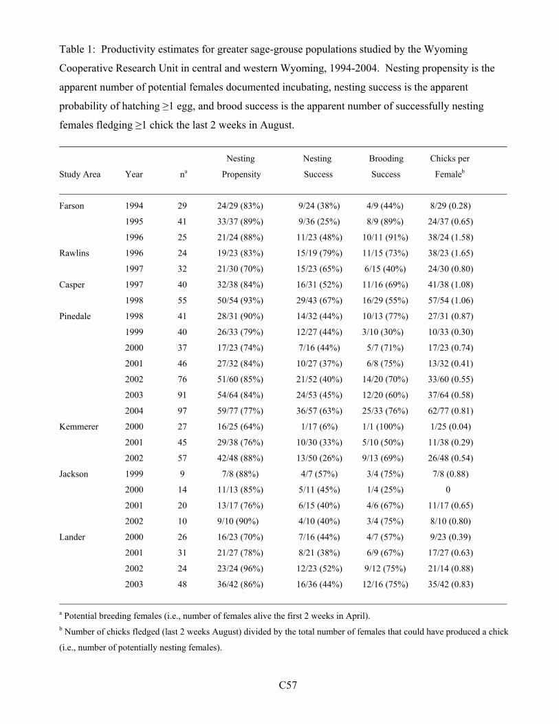
Table 1: Productivity estimates for greater sage-grouse populations studied by the Wyoming

Cooperative Research Unit in central and western Wyoming, 1994-2004. Nesting propensity is the

apparent number of potential females documented incubating, nesting success is the apparent

probability of hatching ≥1 egg, and brood success is the apparent number of successfully nesting

females fledging ≥1 chick the last 2 weeks in August.

Nesting Nesting Brooding Chicks per

Study Area Year na Propensity Success Success Femaleb

Farson 1994 29 24/29 (83%) 9/24 (38%) 4/9 (44%) 8/29 (0.28)

1995 41 33/37 (89%) 9/36 (25%) 8/9 (89%) 24/37 (0.65)

1996 25 21/24 (88%) 11/23 (48%) 10/11 (91%) 38/24 (1.58)

Rawlins 1996 24 19/23 (83%) 15/19 (79%) 11/15 (73%) 38/23 (1.65)

1997 32 21/30 (70%) 15/23 (65%) 6/15 (40%) 24/30 (0.80)

Casper 1997 40 32/38 (84%) 16/31 (52%) 11/16 (69%) 41/38 (1.08)

1998 55 50/54 (93%) 29/43 (67%) 16/29 (55%) 57/54 (1.06)

Pinedale 1998 41 28/31 (90%) 14/32 (44%) 10/13 (77%) 27/31 (0.87)

1999 40 26/33 (79%) 12/27 (44%) 3/10 (30%) 10/33 (0.30)

2000 37 17/23 (74%) 7/16 (44%) 5/7 (71%) 17/23 (0.74)

2001 46 27/32 (84%) 10/27 (37%) 6/8 (75%) 13/32 (0.41)

2002 76 51/60 (85%) 21/52 (40%) 14/20 (70%) 33/60 (0.55)

2003 91 54/64 (84%) 24/53 (45%) 12/20 (60%) 37/64 (0.58)

2004 97 59/77 (77%) 36/57 (63%) 25/33 (76%) 62/77 (0.81)

Kemmerer 2000 27 16/25 (64%) 1/17 (6%) 1/1 (100%) 1/25 (0.04)

2001 45 29/38 (76%) 10/30 (33%) 5/10 (50%) 11/38 (0.29)

2002 57 42/48 (88%) 13/50 (26%) 9/13 (69%) 26/48 (0.54)

Jackson 1999 9 7/8 (88%) 4/7 (57%) 3/4 (75%) 7/8 (0.88)

2000 14 11/13 (85%) 5/11 (45%) 1/4 (25%) 0

2001 20 13/17 (76%) 6/15 (40%) 4/6 (67%) 11/17 (0.65)

2002 10 9/10 (90%) 4/10 (40%) 3/4 (75%) 8/10 (0.80)

Lander 2000 26 16/23 (70%) 7/16 (44%) 4/7 (57%) 9/23 (0.39)

2001 31 21/27 (78%) 8/21 (38%) 6/9 (67%) 17/27 (0.63)

2002 24 23/24 (96%) 12/23 (52%) 9/12 (75%) 21/14 (0.88)

2003 48 36/42 (86%) 16/36 (44%) 12/16 (75%) 35/42 (0.83)

a Potential breeding females (i.e., number of females alive the first 2 weeks in April). b Number of chicks fledged (last 2 weeks August) divided by the total number of females that could have produced a chick

(i.e., number of potentially nesting females).

C57

Figure 1: Study area locations for greater sage-grouse research projects conducted by the Wyoming

Cooperative Research Unit, 1994-2005. Consult the text for study area description corresponding to

numbers present on map. Inset map (Connelly et al. 2004) outlines sage-grouse breeding population

strongholds as of 2003; the darkest shades represent the greatest densities of males / km2.

C58

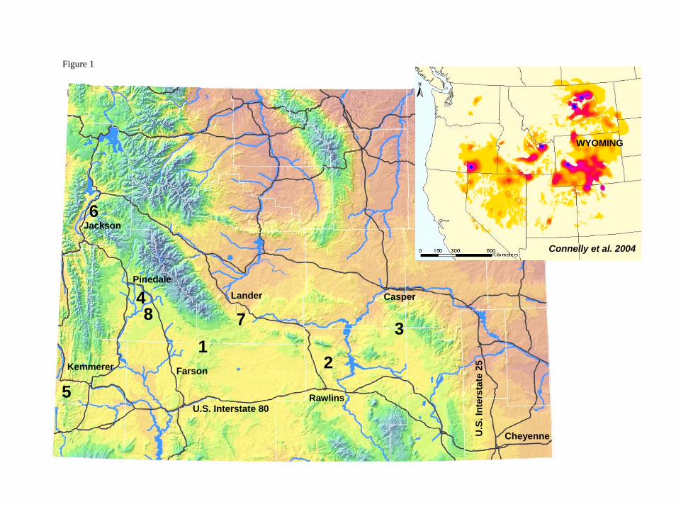
Figure 1

Cheyenne

U.S. Interstate 80

Casper

U.S

. Int

erst

ate

25

Lander

Rawlins

Farson

Pinedale

Jackson

Kemmerer

1

6

84

5

7

2

3

WYOMING

Connelly et al. 2004

Documents

GREATER SAGE-GROUSE (Centrocercus urophasianus) … · 1 Holloran, Matthew J., Greater Sage-Grouse (Centrocercus urophasianus) Population Response to Natural Gas Field Development