Embed Size (px)
Citation preview
Lake Eyre Basin Springs Assessment
Great Artesian Basin spring wetland area mapping and flow estimation
DEWNR Technical report 2015/54

Lake Eyre Basin Springs Assessment
Great Artesian Basin spring wetland area
mapping and flow estimation
Prepared for
The Department of Environment, Water and Natural Resources
By
Davina White, Brooke Schofield & Megan Lewis
School of Biological Sciences
The University of Adelaide
Adelaide, 5005
September 2015
Department of Environment, Water and Natural Resources
GPO Box 1047, Adelaide SA 5001
Telephone National (08) 8463 6946
International +61 8 8463 6946
Fax National (08) 8463 6999
International +61 8 8463 6999
Website www.environment.sa.gov.au
Disclaimer
The Department of Environment, Water and Natural Resources and its employees do not warrant or make
any representation regarding the use, or results of the use, of the information contained herein as regards
to its correctness, accuracy, reliability, currency or otherwise. The Department of Environment, Water and
Natural Resources and its employees expressly disclaims all liability or responsibility to any person using
the information or advice. Information contained in this document is correct at the time of writing.
This work is licensed under the Creative Commons Attribution 4.0 International License.
To view a copy of this license, visit http://creativecommons.org/licenses/by/4.0/.
ISBN 978-1-925369-39-7
Preferred way to cite this publication
White D, Schofield B and Lewis M, 2015, Great Artesian Basin spring wetland area mapping and flow
estimation, DEWNR Technical report 2015/54, report by the University of Adelaide to the Government of
South Australia, through Department of Environment, Water and Natural Resources, Adelaide
Download this document at: http://www.waterconnect.sa.gov.au

Acknowledgements
The Lake Eyre Basin Springs Assessment (LEBSA) project received valuable guidance from the
project Technical Reference Committee members made up of members from various offices,
departments and groups and of diverse backgrounds, including the Department of Environment
(DE), Bureau of Meteorology (BoM), Geoscience Australia (GA), Queensland Department of
Science, Information Technology, Innovation, and the Arts (DSITIA), the SAAL NRM Board and
the South Australian Department of Environment, Water and Natural Resources (DEWNR).
The LEBSA project has been delivered concurrently and in-conjunction with an equivalent
project run by DSITIA, of which Keryn Oude-egberink (DSITIA LEBSA PM) has been instrumental
in providing feedback to the TRC and SA LEBSA project, and guidance to the many DSITIA staff
working on the project.
Overarching program guidance and coordination of SA and Qld LEBSA projects was provided by
the Executive Steering Committee members: Peter Baker (DE), Edwina Johnson (DE), Anisa
Coric (DE), Kriton Glenn (GA), Tim Evans (GA), Phil Deamer (BoM), Sarah van Rooyen (BoM),
Brendan Moran (BoM), Tom Carrangis (DEWNR), Tim Ryan (DSITIA) and Keryn Oude-egberink
(DSITIA).
The DEWNR LEBSA project team comprised: Andy Harrison (Project Manager), sub-Project
Manager (Danny Brock), Travis Gotch, Ronald Bonifacio, Mel White, Dan Wohling, Mark Keppel,
Dave Armstrong, Glen Scholz, Matt Miles, (DEWNR), with Catherine Miles (Miles Environmental
Consulting) and Katie Fels (Jacobs).

Summary
The remotely sensed methods outlined and implemented in this report achieved the main aims:
(i) to identify and map the extent of the vegetated areas around spring vents to generate date
stamped wetland polygons for spring groups and complexes of interest to LEBSA; and (ii)
calculate the wetland area and flow rates for these spring groups and complexes using ancillary
data from the Lewis et al. (2013) study. Outputs of wetland areas are reported along with a
guide to their interpretation and an example figure to illustrate their range of variability in
extent and spatial distribution. Wetland areas and estimated flow rates for whole spring groups
are provided. Flow rates are provided as a range, based on the regression relationships
developed by White et al. (2015) between wetland extent and flow rate, which encapsulate the
range of natural variability in the wetlands in response to rainfall events, climatic conditions
and historic land management. The wetland extent polygons have also been provided as a
digital record for comparison with any future monitoring programs.
Estimated ranges of spring flow rates are reported, providing a baseline ‘envelope’ against
which any future changes in spring flow rates can be monitored and objectively compared. The
data provided in this report synthesizes existing and new remotely sensed outputs for mapping
and monitoring GAB spring wetland extents and flow rates along its western margin in South
Australia. The methods implemented in this report are designed for monitoring and could be
used to document any future changes in spring wetland extents and associated flow rates due
to mining operations in the region.
i
Table of Contents
Acknowledgements .................................................................................................................... 3
Summary .................................................................................................................................... 4
Table of Contents ........................................................................................................................ i
Figures ........................................................................................................................................ ii
Tables ......................................................................................................................................... ii
1 Introduction ........................................................................................................................... 1
2 Methods .................................................................................................................................. 2
2.1 Study area ......................................................................................................................... 2
2.2 High resolution satellite image data and pre-processing ................................................... 4
2.3 Airborne hyperspectral image data and pre-processing .................................................... 4
2.4 On-ground calibration data collection ............................................................................... 6
2.5 Wetland extent calculations .............................................................................................. 6
2.6 Estimating flow rates ........................................................................................................ 8
2.7 Methodological considerations ......................................................................................... 9
3 Results .................................................................................................................................... 9
3.1 Wetland extents ............................................................................................................... 9
3.2 Flow estimates ................................................................................................................ 11
4. Conclusions and Recommendations ................................................................................... 14
5. References ........................................................................................................................... 17
Appendix 1. Site specific methodological notes for wetland extent calculations .................. 18

ii
Figures
Figure 1. Study area extent and location of South Australian Great Artesian Basin springs
captured with satellite and airborne imagery (modified from Lewis et al., 2013). .......................3
Figure 2. Schematic of image analysis sequence for calculating wetland extents. ........................6
Figure 3. Mapped spatial distribution of spring wetland extents at Hermit Hill Springs Complex.
.................................................................................................................................................11
Tables
Table 1. QuickBird satellite imagery captured for selected sites and waveband specifications
(modified from White et al., 2015). .............................................................................................4
Table 2. Airborne hyperspectral imagery captured for selected sites and waveband
specifications (modified from Lewis et al., 2013, Appendix 2, p. 135). .........................................5
Table 3. Spring group wetland extents in hectares. ...................................................................12
Table 4. Spring group flow estimate ranges in litres per second (best estimate flow rate in
parentheses). ............................................................................................................................13

1
1 Introduction
This report is part of a series of studies forming part of the Lake Eyre Basin Springs
Assessment (LEBSA) project. The LEBSA project is one of three water knowledge
projects undertaken by the South Australian Department of Water, Environment and
Natural Resources (DEWNR) to inform the Bioregional Assessment Programme in the
Lake Eyre Basin (LEB). The three projects are:
Lake Eyre Basin Rivers Monitoring (LEBRM)
Arckaringa Basin and Pedirka Basin Groundwater Assessment
Lake Eyre Basin Springs Assessment (LEBSA)
The Bioregional Assessment Programme is a transparent and accessible programme
of baseline assessments that increase the available science for decision making
associated with potential water-related impacts of coal seam gas (CSG) and large
coal mining (LCM) developments. The coal-bearing Arckaringa, Pedirka, Cooper and
Galilee basins (Figure 1) have been identified as regions where CSG and LCM
developments are likely to occur or increase in the future. Bioregional assessments
are being prepared in the LEB for the four coal regions to strengthen the science
underpinning future decisions about CSG and LCM activities and their impacts on
groundwater quality, surface water resources and aquatic ecosystems.
The objective of the LEBSA project was to address knowledge gaps relating to the
potential impacts of mining developments on groundwater resources and assets
across the LEB. In particular, the project aimed to characterise and attribute aspects
of springs and other GDEs that are critical for the maintenance of those assets (e.g.
ecological, hydrogeological, hydrochemical), in a way that is consistent across South
Australia and Queensland.
For the LEBSA project the South Australian Department of Environment, Water and
Natural Resources (DEWNR) requested further extension and application of the
methods developed by researchers at the University of Adelaide (Lewis et al., 2013)
for quantifying Great Artesian Basin (GAB) spring wetland extents and associated
estimates of groundwater flows. These methods have been peer reviewed and
published in the scientific literature (White and Lewis 2011; White et al., 2015), and
are a robust and repeatable means for spatially computing spring wetland extent
from remotely sensed satellite and airborne imagery. Regression relationships
established between wetland extents and spring flow rates provide a reliable remote
indicator of spring flow for groups of springs distributed over broad landscapes.
These outputs will provide a valuable baseline assessment for the Bioregional
Assessment Programme. The methods are designed for monitoring and can be used

2
to document any future changes in spring wetland extents and associated flow rates
due to mining operations in the region.
Thus, the aims of this study were to:
identify and map the extent of vegetated areas around spring vents to
generate date-stamped wetland polygons for the named spring groups; and
calculate the wetland area and flow rates for spring groups using existing
satellite and airborne imagery and spatial spring vent DGPS data (obtained
during the Allocating Water and Maintaining Springs in the Great Artesian
Basin, National Water Commission project; Lewis et al., 2013), for all sites
included in the study.
Wetland areas and estimated flow rates for whole spring groups are provided. Flow
rates are provided as a range, based on the regression relationships developed by
White et al. (2015) between wetland extent and flow rate, which encapsulate the
range of natural variability in the wetlands in response to rainfall events, climatic
conditions and historic land management.
2 Methods
2.1 Study area
The study area (Figure 1) covers an extensive part of northern South Australia. This
arid region is punctuated with contrasting spring wetlands supported by artesian
water outflow from aquifers on the western margin of the Great Artesian Basin
(GAB). A number of spring groups and complexes have been identified for the LEBSA
that require baseline and continued monitoring in light of proposed mining
operations in the region. The groups and complexes of interest are: Freeling South
Spring Group, Billa Kalina Spring Group, Hawker Spring Group, Levi spring Group,
Fred Spring Group, and all groups in the Hermit Hill Complex, Beresford Hill Complex,
Strangways, and Coward Complex (Figure 1).
Figure 1 provides the location and spatial extent of the spring groups covered by the
satellite and airborne hyperspectral imagery within the study area. Images were
acquired in 2009 and 2011 for the Allocating Water and Maintaining Springs in the
Great Artesian Basin, National Water Commission project (Lewis et al., 2013). The
analyses reported here are based on the 2009 imagery, as this is considered the
most reliable basis for this baseline study; the six preceding years were very dry,
allowing us to infer that wetland extents and flows were almost entirely a result of
GAB groundwater outflow. Lewis et al. (2013) and White et al. (2015) observed that
antecedent rainfall could substantially increase wetland vegetation extents (evident
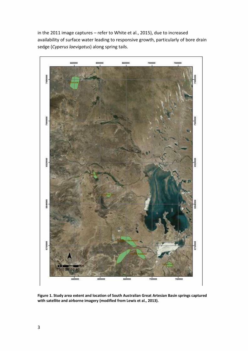
3
in the 2011 image captures – refer to White et al., 2015), due to increased
availability of surface water leading to responsive growth, particularly of bore drain
sedge (Cyperus laevigatus) along spring tails.
Figure 1. Study area extent and location of South Australian Great Artesian Basin springs captured with satellite and airborne imagery (modified from Lewis et al., 2013).

4
2.2 High resolution satellite image data and pre-processing
The mapping of wetland area and estimation of spring flows for Dalhousie Spring
Complex (DSC) used QuickBird high resolution multispectral satellite imagery
acquired in May 2009 (Table 1). The images were provided partially orthorectified
(coarse terrain corrections and projected to a constant base elevation) and partially
radiometrically corrected (DigitalGlobe, 2013). Further geo-registration was
performed to improve positional accuracy for aligning the imagery with field survey
plots (White et al., 2015). Further radiometric correction was conducted to convert
the images to apparent surface reflectance. The satellite scene tiles were
subsequently colour balanced and mosaicked to give full seamless coverage (White
et al., 2015).
Digital colour (red, green and blue) aerial photography at 0.3 m GSD was acquired in
March 2009. The high resolution photography was used to assist with interpretation
of the wetland extent mapping from the satellite image analysis.
Table 1. QuickBird satellite imagery captured for selected sites and waveband specifications (modified from White et al., 2015).
Site Date
captured
GSD* Waveband configuration Band centres used for
NDVI** calculations
DSC 6 May 2009 2.62
m 479.5 nm – blue; 546.5 nm
– green; 654.0 nm – red;
814.5 nm – near-infrared
654.0 nm – red
814.5 nm – near-
infrared
*GSD refers to Ground Sample Distance (equivalent to pixel size at nadir – directly overhead). ** NDVI refers to Normalized Difference Vegetation Index – a measure of vegetation greenness.
2.3 Airborne hyperspectral image data and pre-processing
The remaining spring groups and complexes of interest to LEBSA were covered by
HyMap hyperspectral airborne imagery for the Allocating Water and Maintaining
Springs in the Great Artesian Basin, National Water Commission project; Lewis et al.,
2013 (Table 2). The airborne hyperspectral imagery was provided by HyVista
Corporation with image pre-processing completed, which included atmospheric
correction with the HyCorr model, geometric correction and colour balancing swaths
to form seamless mosaics of each study area (Lewis et al., 2013, Appendix A2.3.1,
pp.132). Full specifications of the hyperspectral imagery are provided in Table 2. The
3 m image pixels of this imagery provided sufficiently fine spatial resolution to

5
delineate individual spring wetlands, while covering a wide range of spring sizes at
the group and complex scale.
This remote sensing study for LEBSA used HyMap imagery flown on 15th – 25th March
2009 (refer to Lewis et al., 2013 report pp. 10), following very dry antecedent
conditions. Thus, the extents of wetlands derived from the 2009 hyperspectral
imagery have a high probability of being influenced only by groundwater flows.
Table 2. Airborne hyperspectral imagery captured for selected sites and waveband specifications (modified from Lewis et al., 2013, Appendix 2, p. 135).
Site
(spring group)
Date
captured
GSD
*
Waveband
configuration
Band centres used
for NDVI**
calculations
Freeling South
15 - 25
March
2009
3 m
126 near contiguous
narrow (~15 nm)
wavebands;
wavelength range
450 - 2,500 nm
665.7 nm - red
847.8 nm - near-
Infrared
All groups
within Hermit
Hill Complex
Billa Kalina
Hawker
Levi
Fred
Strangways
All groups
within
Beresford Hill
Complex
All groups
within Coward
Complex
*GSD refers to Ground Sample Distance (equivalent to pixel size at nadir – directly
overhead).
** NDVI refers to Normalized Difference Vegetation Index – a measure of vegetation
greenness.
Note that no imagery was captured over Gosse Springs, therefore wetland extent
calculations could not be produced for this study.

6
2.4 On-ground calibration data collection
Vegetation cover and composition were recorded between March and April 2009,
within ground survey plots of 9 × 9m, designed to allow for geolocation errors and
geometric accuracy of the imagery, as well as the scale of vegetation stands and
variation. Within the plots, percentage cover of plant species and overall fractions of
photosynthetic vegetation, dry vegetation, water and soil were recorded using the
methods described by Lewis et al. (2013) and White and Lewis (2011). Differential
GPS locations were recorded at the corners of the survey plots to enable their later
identification on the imagery (White et al., 2015). These data were used to derive
regression relationships between image NDVI values and on-ground estimates of
vegetation cover. These relationships were used in mapping and estimating wetland
extent (Section 2.5).
Spring flow data were selected either from ongoing monitoring records or new in-
situ measurements that were made in the Lewis et al. (2013) and White et al. (2015)
studies. The in-situ flow measurements coincided with the vegetation surveys. The
timing of the discharge measurements corresponded as closely as feasible with the
image acquisitions.
2.5 Wetland extent calculations
Calculation of wetland area extents involved the sequence of analyses shown in
Figure 2.
Figure 2. Schematic of image analysis sequence for calculating wetland extents.
Compute spring areas
Individual Spring group
Intercept digitized areas with NDVI threshold
Apply NDVI threshold
Compute image NDVIMask creeks and 'heads-up digitize' around springs of interest
Spatially sub-set around springs of interest
7
The Normalized Difference Vegetation Index (NDVI – a measure of vegetation
greenness) was applied to both the HyMap hyperspectral airborne imagery and the
QuickBird satellite imagery. Tables 1 and 2 summarize the image wavebands used for
the NDVI calculations for all imagery employed (for full derivation of the equations
refer to White and Lewis, 2011; Lewis et al., 2013, pp. 133). The NDVI image outputs
were calibrated using the on-ground survey data comprising vegetation cover and
composition (Lewis et al., 2013; White and Lewis, 2011; White et al., 2015).
Regression relationships were developed between image NDVI values and
corresponding on-ground percentage vegetation cover for each plot surveyed for
three sites in the Lewis et al., 2013 and White et al., 2015 studies (Dalhousie Springs
Complex, Freeling Spring South Group, and Hermit Hill Spring Group). For DSC overall
vegetation cover (photosynthetic and dry vegetation) was used to develop the
regression relationship (White and Lewis, 2011). This approach was refined for
Freeling South Spring Group and Hermit Hill Spring Group where the photosynthetic
vegetation fraction of cover was used for the analyses. From these relationships
NDVI thresholds were determined for each site to separate wetland vegetation from
surrounding dryland vegetation (White et al., 2015). The threshold of importance for
the current reporting for DSC, 0.35, was derived from White and Lewis (2011).
NDVI was also calculated for the HyMap hyperspectral airborne imagery as part of
the Lewis et al. (2013) study for the following sites: Freeling South Springs Group,
and all spring groups in the Hermit Hill Complex (Beatrice, Bopeechee, Bopeechee
Mound, Bopeechee North, Dead Boy, Finniss Well, Hermit Hill, North West, Old
Finniss, Old Woman, Sulphuric, West Finniss). For the current reporting these
analyses were extended to the following sites: Billa Kalina, Hawker, Levi, Fred,
Strangways, all spring groups within the Coward Spring Complex, and all spring
groups within the Beresford Hill Spring Complex. The airborne hyperspectral image
NDVI thresholds were a consistent value of 0.17, derived from Lewis et al. (2013).
This threshold value was appropriate for delineating spring wetland vegetation from
surrounding dryland vegetation at all sites.
The methodology developed by White and Lewis (2011) for DSC was applied with
some site-specific modifications (refer to Appendix 1 for details) to all other spring
groups presented in the current report. The method involved the following steps:
(i) the extent of spring groups was broadly delineated by heads-up digitising on the
NDVI threshold imagery;
(ii) where spring groups were more difficult to delineate, their associated wetlands
were distinguished using a suite of ancillary data, including spring vent DGPS
coordinates and codes (Gotch, 2010; Lewis et al., 2013), and expert knowledge of the
sites;
8
(iii) polygons produced from the digitising were intersected with the NDVI threshold
image to produce precise delineations of wetland extent for the spring groups of
interest; and
(iv) spring group wetland areas were calculated in hectares.
2.6 Estimating flow rates
White et al. (2015) developed strong positive linear regression relationships between
spring wetland area and discharge at the individual spring level for all three sites
they investigated (DSC R2 = 0.99; FSG R2 = 0.95; HHSG R2 = 0.92; p < 0.001 in all cases;
refer to White et al., (2015) for details. Differences in the relationships between the
sites captured variability primarily due to differences in antecedent conditions
(rainfall driven), site specific geomorphological and hydrogeological settings and lags
between on-ground calibration data and image capture (for Hermit Hill Spring
Group) as reported by Lewis et al. (2013) and White et al. (2015). The regression
relationships developed by White et al. (2015) were used for the LEBSA spring flow
estimates:
DSC: 𝑦 = 1.21𝑥 + 0
Hermit Hill Spring Group: 𝑦 = 0.68𝑥 + 0
Freeling South Spring Group: 𝑦 = 2.58𝑥 + 0
where y is wetland area and x is spring flow.
However, analysis of covariance (ANCOVAR) indicated that the slopes of the three
regression lines for the three sites are not significantly different. A very strong
positive linear regression relationship was also apparent between spring wetland
area and discharge for all sites combined (R2 = 0.99 p<0.001) (White et al., 2015).
For the purposes of this report a range of estimated spring flow rates is provided to
capture the variations mentioned above: these values are based on the White et al.
(2015) regression relationships outlined above. The shallower slope for Hermit Hill
Spring Group is most likely due to a lag of eight weeks between the collection of on-
ground calibration data and image capture. The spring wetland vegetation over the
eight week period senesced, resulting in lower NDVI values recorded in the captured
imagery relative to on-ground vegetation cover. Therefore, the higher flow rates
resulting from calculations using this lower slope in the regression equation are likely
to be an over-estimate of actual flow values. To address this likely over-estimation
we have provided the full range of possible flow values in Table 4, the value in
parentheses represents the estimated flow rate from the DSC slope of 1.21. We

9
provide our interpretation of the most probable flow rate range for each LEBSA site
investigated in section 3.2.
2.7 Methodological considerations
The methods presented in this report are reliable, robust and repeatable and have
been peer-reviewed and published in the scientific literature. There are a number of
decisions we have made concerning the methods for deriving the spring wetland
extents and their associated flow measurements, which are explained below to
assist with interpretation of the results presented in Section 3.
Spring wetland extents have been calculated at the spring group scale where
spring inter-connectivity is extensive and delineation of individual springs
would therefore be impractical.
The range of spring flow rates captured in the White et al. (2015) study
demonstrates the range of natural variability of the springs in response to
rainfall and climatic conditions. The estimated spring flow rates have been
presented as ranges and the most likely location within the range provided in
the interpretation of these results. The envelope defined by this range could
be considered a baseline natural flow regime, within which the springs are
currently performing.
There are differences in the NDVI thresholds applied to spring group and
complex sites, where different remotely sensed imagery was used to
calculate NDVI. These differing values are largely the result of image band
widths. All imagery was calibrated to at-surface reflectance enabling
comparison between sites, dates and image types. Consequently wetland
mapping and area estimations are comparable between image types.
3 Results
This section provides the results of the image analyses to determine wetland
extents, derived from delineating spring wetlands from NDVI thresholds applied to
the high resolution satellite imagery (DSC) and hyperspectral imagery (all other
sites). Spring flow rate estimates are derived from the wetland area to flow
regression equations outlined in section 2.6.
3.1 Wetland extents
The wetland extents calculated for all LEBSA spring sites of interest are summarized
in Table 3. The spring wetland extents differ considerably between groups and within
complexes. DSC has the largest overall wetland extent at 913 ha, followed by the
Hermit Hill Springs Complex 39 ha, Coward springs Complex 15.72 ha, and Beresford

10
Hill Springs Complex 2.11 ha. Spring group wetland extents vary most widely at the
Hermit Hill Springs Complex, ranging between 12.93 and 0.12 ha, for Hermit Hill
Springs Group and Bopeechee Mound Springs Group, respectively. Overall, the most
extensive wetland area associated with a single spring group is Hawker at 14.86 ha,
the least extensive is Secret (BSS) at 0.001 ha.
For Strangways and Billa Kalina Spring Groups further ancillary data is required to
provide more accurate and robust calculations of wetland extent, i.e., DGPS
measurements of vent activity (extinct, active, damp) to locate all springs with
associated wetland vegetation within these groups. Remotely sensed imagery is not
available for Gosse Springs, so no calculations of wetland extent could be conducted
for this site.
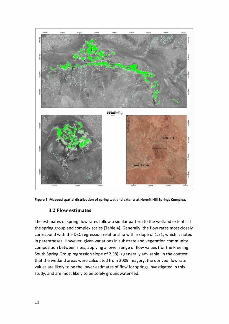
An example of mapped outputs illustrating the wetland extents and their spatial
variability and inter-connectivity within two spring complexes is provided in Figure 3.
11
Figure 3. Mapped spatial distribution of spring wetland extents at Hermit Hill Springs Complex.
3.2 Flow estimates
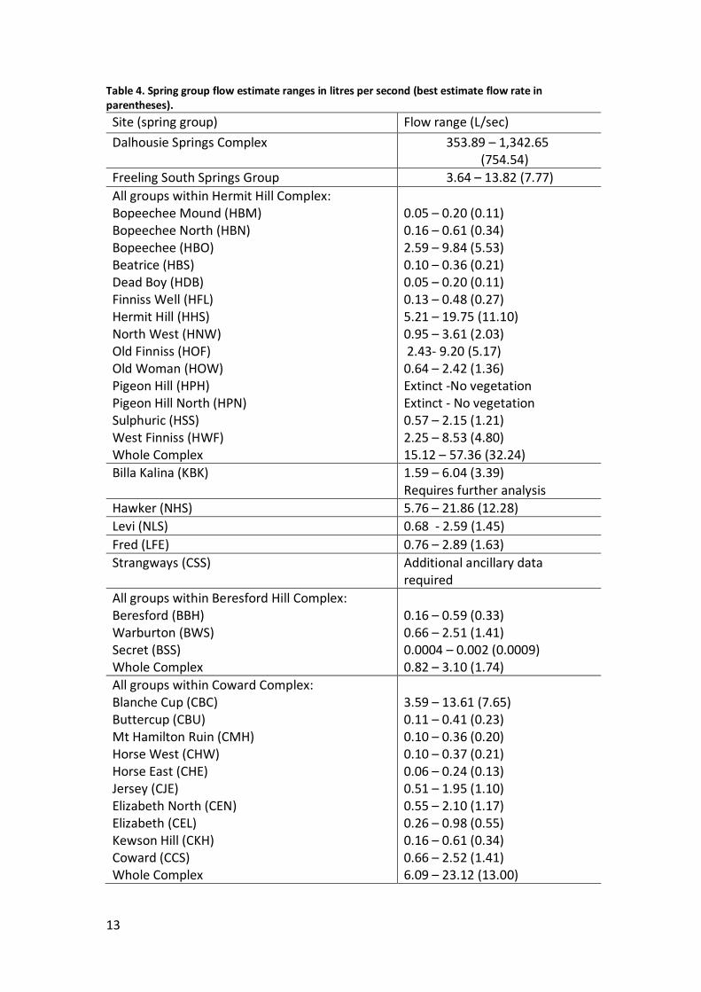
The estimates of spring flow rates follow a similar pattern to the wetland extents at
the spring group and complex scales (Table 4). Generally, the flow rates most closely
correspond with the DSC regression relationship with a slope of 1.21, which is noted
in parentheses. However, given variations in substrate and vegetation community
composition between sites, applying a lower range of flow values (for the Freeling
South Spring Group regression slope of 2.58) is generally advisable. In the context
that the wetland areas were calculated from 2009 imagery, the derived flow rate
values are likely to be the lower estimates of flow for springs investigated in this
study, and are most likely to be solely groundwater-fed.

12
Table 3. Spring group wetland extents in hectares.
Site(spring group) Wetland area (ha)
Dalhousie Springs Complex (DSC) 913
Freeling South Springs Group 9.4
All groups within Hermit Hill Complex: Beatrice (HBS) Bopeechee (HBO) Bopeechee Mound (HBM) Bopeechee North (HBN) Dead Boy (HDB) Finniss Well (HFL) Hermit Hill (HHS) North West (HNW) Old Finniss (HOF) Old Woman (HOW) Sulphuric (HSS) West Finniss (HWF) Pigeon Hill (HPH) Pigeon Hill North (HPN) Whole Complex
0.19 3.83 0.12 0.23 0.13 0.23 12.93 2.46 6.20 1.57 1.31 5.74 Extinct – No vegetation Extinct – No vegetation 39.00
Billa Kalina (KBK) 4.11*
Hawker (NHS) 14.86
Levi (NLS) 1.76
Fred (LFE) 1.97
Strangways (CSS) Additional ancillary data
required*
All groups within Beresford Hill Complex: Beresford (BBH) Warburton (BWS) Secret (BSS) Whole Complex
0.40 1.70 0.001 2.11
All groups within Coward Complex: Blanche Cup (CBC) Buttercup (CBU) Mt Hamilton Ruin (CMH) Horse West (CHW) Hose East (CHE) Jersey (CJE) Elizabeth North (CEN) Elizabeth (CEL) Kewson Hill (CKH) Coward (CCS) Whole Complex
9.26 0.28 0.25 0.25 0.16 1.33 1.41 0.66 0.41 1.71 15.72
* Requires further analysis
13
Table 4. Spring group flow estimate ranges in litres per second (best estimate flow rate in parentheses).
Site (spring group) Flow range (L/sec)
Dalhousie Springs Complex 353.89 – 1,342.65 (754.54)
Freeling South Springs Group 3.64 – 13.82 (7.77)
All groups within Hermit Hill Complex: Bopeechee Mound (HBM) Bopeechee North (HBN) Bopeechee (HBO) Beatrice (HBS) Dead Boy (HDB) Finniss Well (HFL) Hermit Hill (HHS) North West (HNW) Old Finniss (HOF) Old Woman (HOW) Pigeon Hill (HPH) Pigeon Hill North (HPN) Sulphuric (HSS) West Finniss (HWF) Whole Complex
0.05 – 0.20 (0.11) 0.16 – 0.61 (0.34) 2.59 – 9.84 (5.53) 0.10 – 0.36 (0.21) 0.05 – 0.20 (0.11) 0.13 – 0.48 (0.27) 5.21 – 19.75 (11.10) 0.95 – 3.61 (2.03) 2.43- 9.20 (5.17) 0.64 – 2.42 (1.36) Extinct -No vegetation Extinct - No vegetation 0.57 – 2.15 (1.21) 2.25 – 8.53 (4.80) 15.12 – 57.36 (32.24)
Billa Kalina (KBK) 1.59 – 6.04 (3.39) Requires further analysis
Hawker (NHS) 5.76 – 21.86 (12.28)
Levi (NLS) 0.68 - 2.59 (1.45)
Fred (LFE) 0.76 – 2.89 (1.63)
Strangways (CSS) Additional ancillary data required
All groups within Beresford Hill Complex: Beresford (BBH) Warburton (BWS) Secret (BSS) Whole Complex
0.16 – 0.59 (0.33) 0.66 – 2.51 (1.41) 0.0004 – 0.002 (0.0009) 0.82 – 3.10 (1.74)
All groups within Coward Complex: Blanche Cup (CBC) Buttercup (CBU) Mt Hamilton Ruin (CMH) Horse West (CHW) Horse East (CHE) Jersey (CJE) Elizabeth North (CEN) Elizabeth (CEL) Kewson Hill (CKH) Coward (CCS) Whole Complex
3.59 – 13.61 (7.65) 0.11 – 0.41 (0.23) 0.10 – 0.36 (0.20) 0.10 – 0.37 (0.21) 0.06 – 0.24 (0.13) 0.51 – 1.95 (1.10) 0.55 – 2.10 (1.17) 0.26 – 0.98 (0.55) 0.16 – 0.61 (0.34) 0.66 – 2.52 (1.41) 6.09 – 23.12 (13.00)

14
4. Conclusions and Recommendations
For springs in the LEBSA region the outputs of wetland extent and estimated flow
rates from remotely sensed imagery presented in this report provide an excellent
baseline for assessing potential future changes in flow rates in response to climatic
conditions and mining operations. Any changes to wetland extent and flow rates can
be assessed in an objective and reliable way, enabling future monitoring to be
conducted easily, efficiently and objectively, using the methods outlined in this
report. This section provides guidelines on interpretation of the image outputs for
wetland extent and estimated spring flows as well as recommendations for using
these data for future studies and improvements for future work.
The outputs provided in this report have been produced by remote sensing scientists
along with input from spring experts. We recommend the following guidelines for
interpreting these outputs.
The wetland extents are specific to the time of image data capture in 2009
and should be interpreted in the context that they are at the lower end of the
range of wetland extents. The main rationale is that the 2009 images were
captured after a prolonged dry period of six years, and the wetland extents
represent groundwater fed-wetlands, without surface rainfall influences.
Where one very large spring dominates a spring group wetland extent it can
have a major influence on the wetland extent of the whole spring group or
complex. It is therefore important to consider any impacts to springs which
are particularly extensive within a group or complex, in which case any
changes in wetland extent should be closely monitored.
The range of flow rate estimates should be interpreted as a guide to flows at
the springs mapped. We recommend using the lower range values up to the
Dalhousie regression slope values (1.21) in parentheses. The higher values
are likely to be an over-estimate based on the Hermit Hill regression
equation, which has a shallower slope. This is largely due to drying of the
wetland vegetation prior to image capture and the eight week lag between
on-ground calibration data collection and image capture.
These estimates of wetland area and spring flows represent one epoch in
time. The springs are dynamic naturally-occurring features in the arid
landscape. Future rainfall, climatic and land use impacts will all influence the
wetland extent and flow values.
Wetland extent and flow rate estimates have not been provided for the following
spring groups, either because they were not outlined in the project definition or
there is insufficient data for the analyses: Billa Kalina, Strangways, Gosse, Welcome,
McEwins, Francis Swamp, Freeling Springs North. The methods employed in this

15
study are ideal for monitoring any future changes in spring wetland extents and
associated flow rates due to mining operations or other land use impacts and aquifer
pressure changes in the region. The baseline data generated in this study could be
used with future comparable information for monitoring of the springs in the
western margin of the GAB.
We recommend that the methods presented in this report, which have been peer-
reviewed and published in the scientific literature, are implemented to monitor
future changes in spring wetland extents and flow rates in the LEBSA region. The
following specific recommendations are provided for end users to make the best use
of these data for alignment with other projects within the LEB and for future
reporting and monitoring.
Adoption of remote sensing wetland area mapping in future will enable time
series of comparable data to be built up, allowing objective assessment of
changes in the spatial distribution and extent of spring wetlands. Methods
developed by White and Lewis (2011) for detecting and quantifying changes
in wetland extents at DSC using high resolution satellite imagery are suitable
for wider implementation for springs within the western margin of the GAB
using existing hyperspectral airborne imagery captured in 2011 (Lewis et al.,
2013). This approach would enable differences in wetland extents to be
quantified and changes in their spatial distribution to be mapped with
confidence.
If future monitoring identifies spring flows that fall outside the ranges
estimated here, then at the very least further investigation should be
undertaken to determine the cause of the change in spring flow.In addition,
the methods used in this study could also be applied to other water flows,
seepage or leakage from bores and pipes that draw on GAB artesian water,
where such flows support wetland vegetation. For example, the extensive
wetland supported by uncontrolled artesian flows from Big Blyth Bore to the
east of Freeling Springs was mapped in April 2011 using high resolution
satellite imagery and the methods presented in this report (White et al. 2013,
p 57). Since then Big Blyth Bore has been capped. A repeat image-based
study could confirm reduction in the wetlands associated with the bore, and
allow assessment of any change at Freeling Springs as a result of increased
local aquifer pressure.
In addition, the methods used in this study could also be applied to other
water flows, seepage or leakage from bores and pipes that draw on GAB
artesian water, where such flows support wetland vegetation. For example,
the extensive wetland supported by uncontrolled artesian flows from Big
Blyth Bore to the east of Freeling Springs was mapped in April 2011 using

16
high resolution satellite imagery and the methods presented in this report
(White et al. 2013, p 57). Since then Big Blyth Bore has been capped. A repeat
image-based study could confirm reduction in the wetlands associated with
the bore, and allow assessment of any change at Freeling Springs as a result
of increased local aquifer pressure.

17
5. References
Gotch, T.B., 2010. Great Artesian Basin Springs of South Australia: Spatial
Distribution and Elevation Map. South Australia Arid Lands Natural Resources
Management Board, Adelaide, Australia (last Updated June 2010).
Lewis, M.M., White, D.C. & Gotch, T.B. (Eds.) 2013, Allocating Water and Maintaining
Springs in the Great Artesian Basin, Volume IV: Spatial Survey and Remote Sensing of
Artesian Springs of the Western Great Artesian Basin, National Water Commission,
Canberra. ISBN: 978-1-922136-09-1.
White, D.C. and Lewis, M.M., 2011, A new approach to monitoring spatial
distribution and dynamics of wetlands and associated flows of Australian Great
Artesian Basin springs using QuickBird satellite imagery. J. Hydrol. 408, 140-152,
http://dx.doi.org/10.1016/j.hydrol.2011.07.032.
White, D.C., Gotch, T.B., Alaak, Y., Clark, M., Ryan, J. and Lewis, M.M. 2013.
Characterising spring groups. In Lewis, M.M., White, D.C. & Gotch, T.G. (Eds.).
Allocating Water and Maintaining Springs of the Western Great Artesian Basin.
Volume IV. Spatial Survey and Remote Sensing of Artesian Springs of the Western
Great Artesian Basin. National Water Commission, Canberra. ISBN: 978-1-922136-09-
1.
White, D.C., Lewis, M.M., Green, G. and Gotch, T.B. 2015, A generalizable NDVI-
based wetland delineation indicator for remote monitoring of groundwater flows in
the Australian Great Artesian Basin. Ecol. Indic., Special Issue: Spatial Indicators, In
Press. Open Access, http://dx.doi.org/10.1016/j.ecolind.2015.01.032.
Williams, A.F. and Holmes, J.W. 1978, A novel method of estimating the discharge of
water from mound springs of the Great Artesian Basin, Central Australia. J. Hydrol.
38, 263-272, http://dx.doi.org/10.1016/0022-1694(78)90073-2.

18
Appendix 1. Site specific methodological notes for wetland extent calculations
Site: Hawker
The ‘individual’ method was used at Hawker. 99/105 springs had associated wetland
vegetation. In three instances pairs of springs (NHS001/NHS002, NHS080/NHS081,
NHS090/NHS091) were combined because they could not be individually delineated;
their wetlands were too intermingled.
Site: Levi
Levi consists of 13 springs. However, many of them are located near creek beds. If a
grouping method had been applied much of that creek vegetation would have been
included. Therefore, the spring wetlands were individually identified to reduce the
amount of surrounding vegetation.
The wetland identified for one spring (NLS011) may have been a slight over-
estimate: the mapped vegetation may include dryland vegetation proximal to the
vent.
The master copy of DGPS locations was used at Levi rather than creating a
spreadsheet with only the Levi vents.
Site: Fred
Both the ‘grouping’ and ‘individual’ methods were applied at Fred and both resulted
in very similar wetland areas (equal to 2 decimal places). The wetlands were very
easy to define and there was no surrounding dry land vegetation present.
Only 8 springs but they’re very close with intertwined wetlands. Therefore individual
spring wetland extents may not be correct. However, the total wetland area for the
site should be accurate.
The individual regions of interest created for the Levi springs can be
used/intersected with different thresholds. Took care to include the entire spring
environment/extent, even if no vegetation was present (vegetation may appear
there if threshold is lowered).
Site: Hermit Hill
Separate spring groups were identified for Hermit Hill rather than individual springs.
So the method was considered as a ‘grouping’ technique since multiple springs were
identified at a time. There are too many individual springs in close proximity to apply
the individual method.
Deleted the Venebles spring (HVS) from the Hermit Hill Complex. Extinct so doesn’t
need to be mapped.

19
Site: Beresford Hill
Beresford Hill was done in addition to other sites (although wasn’t included in
project brief). It was located within the Strangways imagery and consisted of only a
few springs.
Three separate spring groups were identified for Beresford Hill rather than individual
springs. So the method was considered as a ‘grouping’ technique since multiple
springs were identified at a time. All of the vegetation near the springs was
considered wetland so a grouping method could be applied accurately to this site. An
‘individual’ method was not necessary as accurate results were already achieved
with the grouping method.
Site: Billa Kalina
The ‘individual’ method was applied at Billa Kalina because there was considerable
dryland vegetation present in between springs which would have been included if
springs were grouped. Identified all springs in individual regions of interest (in case
different thresholds were applied) but only those with vegetation were intersected
and further processed.
There were a few springs where it was difficult to distinguish between wetland and
surrounding dryland vegetation. These springs are noted on the spreadsheet. Some
springs were merged because their tails were intermingled.
Only active vents have been included in the wetland extent calculation.
DGPS data is still required for a number of springs at this site, so the wetland extents
and estimated flows are likely lower than for the whole group. It is too difficult at
this stage to delineate all of the springs without the additional DGPS points for the
vents remaining to be mapped.
Site: Strangways
Require more details on vent records, to determine which springs are active. This
additional data is still required as the current data is inconsistent.
There was considerable dryland and creek vegetation surrounding/ proximal to the
spring vents. Even with the true colour imagery displayed, it was very difficult to
decide whether it was spring related or not.
The overall results for Strangways were not considered accurate due to the difficulty
of this site. Further knowledge of the site and ground data might be required to
identify the distribution of wetland and dryland vegetation
20
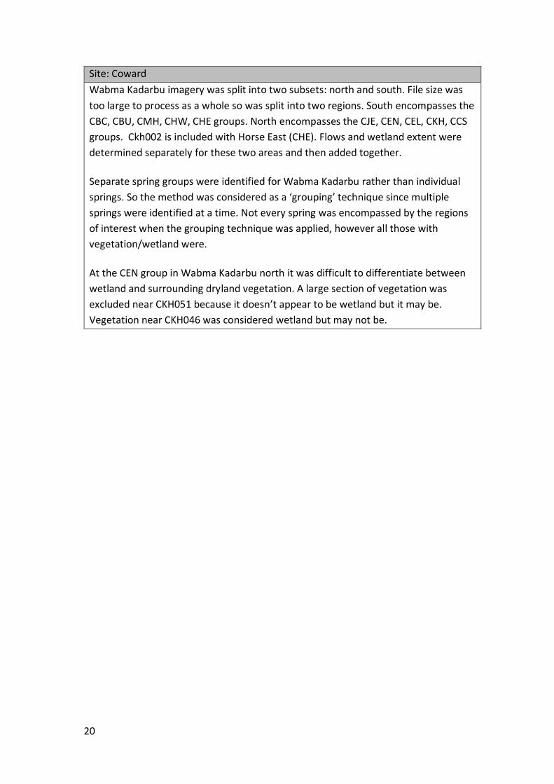
Site: Coward
Wabma Kadarbu imagery was split into two subsets: north and south. File size was
too large to process as a whole so was split into two regions. South encompasses the
CBC, CBU, CMH, CHW, CHE groups. North encompasses the CJE, CEN, CEL, CKH, CCS
groups. Ckh002 is included with Horse East (CHE). Flows and wetland extent were
determined separately for these two areas and then added together.
Separate spring groups were identified for Wabma Kadarbu rather than individual
springs. So the method was considered as a ‘grouping’ technique since multiple
springs were identified at a time. Not every spring was encompassed by the regions
of interest when the grouping technique was applied, however all those with
vegetation/wetland were.
At the CEN group in Wabma Kadarbu north it was difficult to differentiate between
wetland and surrounding dryland vegetation. A large section of vegetation was
excluded near CKH051 because it doesn’t appear to be wetland but it may be.
Vegetation near CKH046 was considered wetland but may not be.