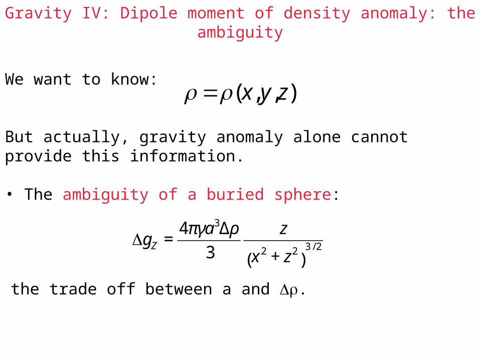
Gravity IV: Dipole moment of density anomaly: the ambiguity

We want to know:

But actually, gravity anomaly alone cannot provide this information.

• The ambiguity of a buried sphere:

€

ΔgZ =4πγa3Δρ

3

z

x 2 + z2( )

3 / 2 .

Note the trade off between a and Δ.

€

=(x,y,z).

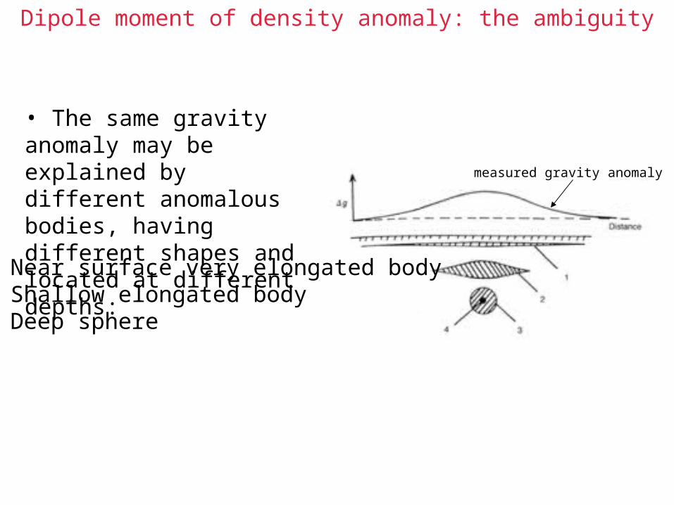
Dipole moment of density anomaly: the ambiguity

1. Near surface very elongated body2. Shallow elongated body3. Deep sphere

• The same gravity anomaly may be explained by different anomalous bodies, having different shapes and located at different depths:

measured gravity anomaly

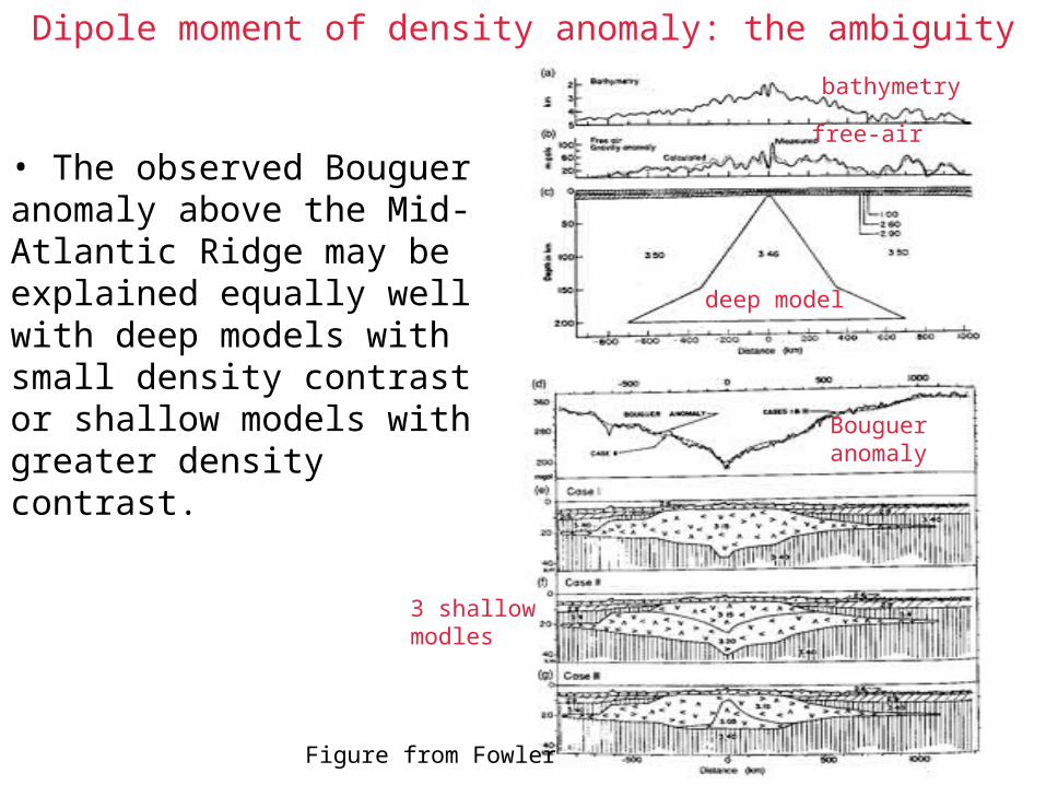
Dipole moment of density anomaly: the ambiguity

• The observed Bouguer anomaly above the Mid-Atlantic Ridge may be explained equally well with deep models with small density contrast or shallow models with greater density contrast.

bathymetry

free-air

deep model

Bougueranomaly

3 shallowmodles

Figure from Fowler

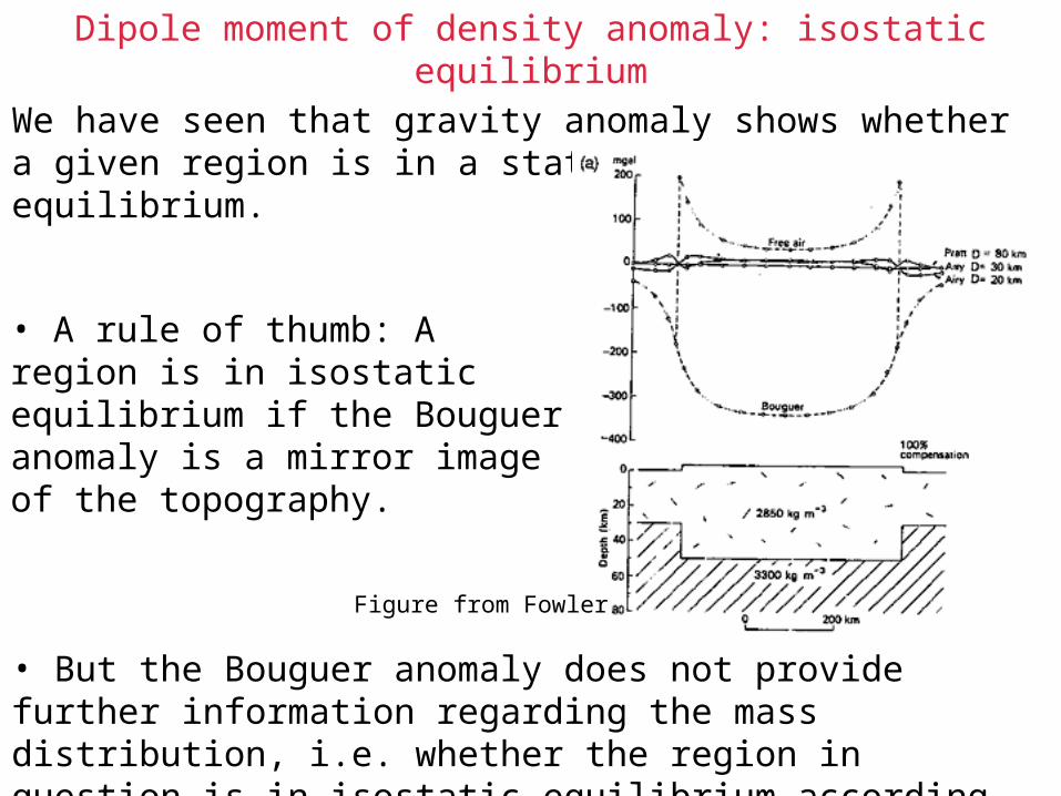
Dipole moment of density anomaly: isostatic equilibrium

We have seen that gravity anomaly shows whether a given region is in a state of isostatic equilibrium.

• A rule of thumb: A region is in isostatic equilibrium if the Bouguer anomaly is a mirror image of the topography.

Figure from Fowler

• But the Bouguer anomaly does not provide further information regarding the mass distribution, i.e. whether the region in question is in isostatic equilibrium according to Airy or Pratt hypotheses?

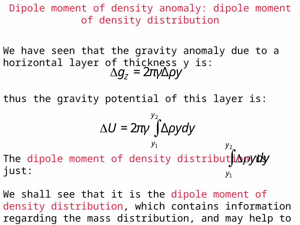
Dipole moment of density anomaly: dipole moment of density distribution

We have seen that the gravity anomaly due to a horizontal layer of thickness y is:

thus the gravity potential of this layer is:

The dipole moment of density distribution is just:

€

ΔgZ = 2πγΔρy ,

€

ΔU = 2πγ Δρydyy1

y2

∫ .

€

Δydyy1

y2

∫ .

We shall see that it is the dipole moment of density distribution, which contains information regarding the mass distribution, and may help to discriminate between the two isostatic models.

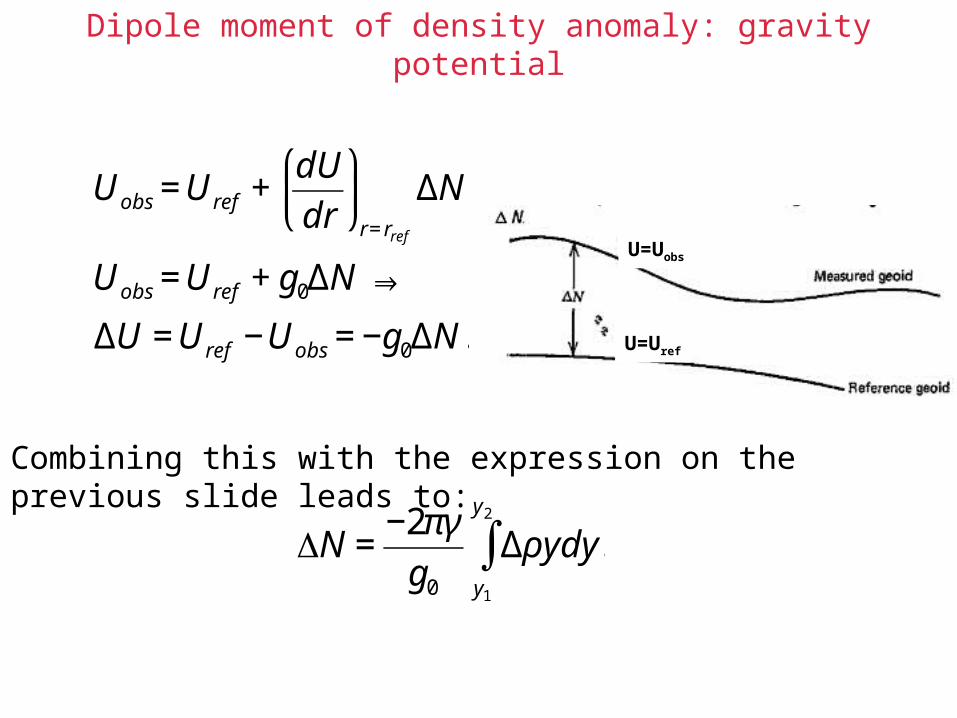
Dipole moment of density anomaly: gravity potential

€

Uobs =Uref +dU

dr

⎛

⎝ ⎜

⎞

⎠ ⎟r= rref

ΔN

Uobs =Uref + g0ΔN ⇒

ΔU =Uref −Uobs = −g0ΔN.

Combining this with the expression on the previous slide leads to:

€

ΔN =−2πγ

g0

Δρydy.y1

y2

∫

U=Uobs

U=Uref

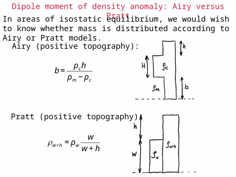
Dipole moment of density anomaly: Airy versus Pratt

Airy (positive topography):

Pratt (positive topography):€

b =ρ ch

ρm − ρ c .

€

w+h = ρww

w + h .

In areas of isostatic equilibrium, we would wish to know whether mass is distributed according to Airy or Pratt models.

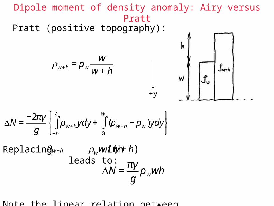
Dipole moment of density anomaly: Airy versus Pratt

Pratt (positive topography):

€

w+h = ρww

w + h .

€

ΔN =−2πγ

gρw+hydy

−h

0

∫ + (ρw+h − ρw )ydy0

w

∫ ⎧ ⎨ ⎩

⎫ ⎬ ⎭ .

Replacing with leads to:

Note the linear relation between ΔN and h.

€

ΔN =πγ

gρwwh .

€

w+h

€

ww /(w + h)

+y

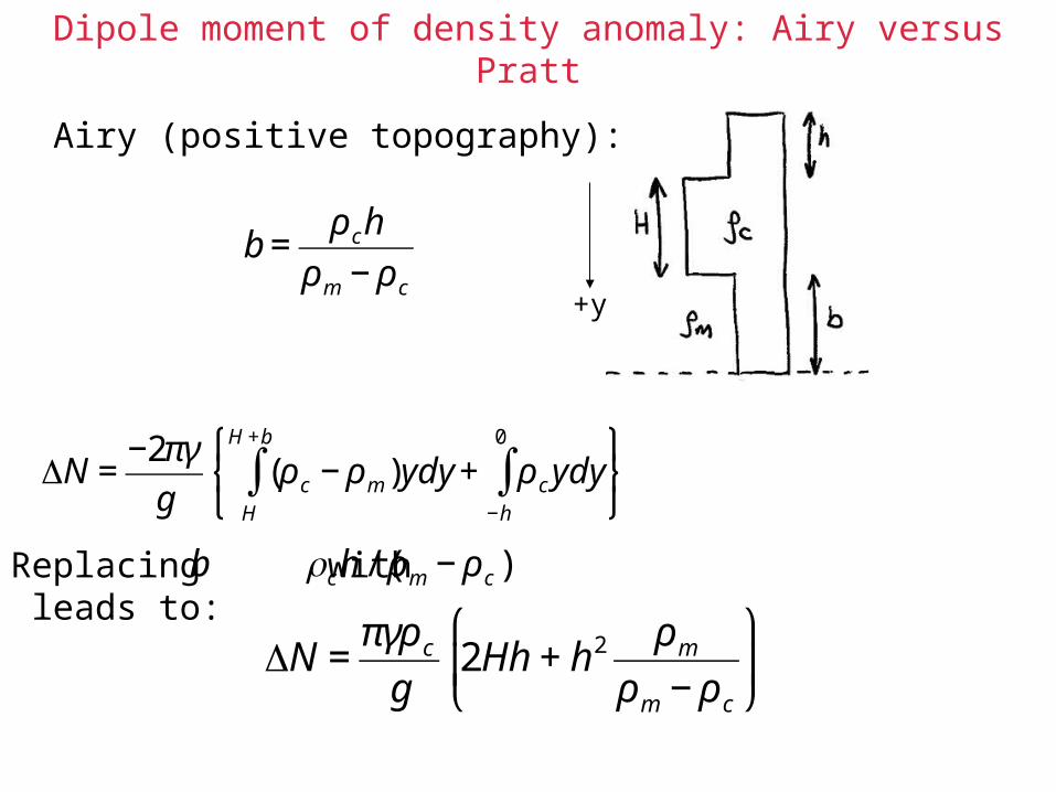
Dipole moment of density anomaly: Airy versus Pratt

Airy (positive topography):

€

b =ρ ch

ρm − ρ c .

+y

€

ΔN =−2πγ

g(ρ c − ρm )ydy

H

H +b

∫ + ρ cydy−h

0

∫ ⎧ ⎨ ⎩

⎫ ⎬ ⎭ .

Replacing with leads to:

Note the NON-LINEAR relation between ΔN and h.

€

ΔN =πγρ cg

2Hh + h2 ρmρm − ρ c

⎛

⎝ ⎜

⎞

⎠ ⎟ .

€

b

€

ch /(ρm − ρ c )

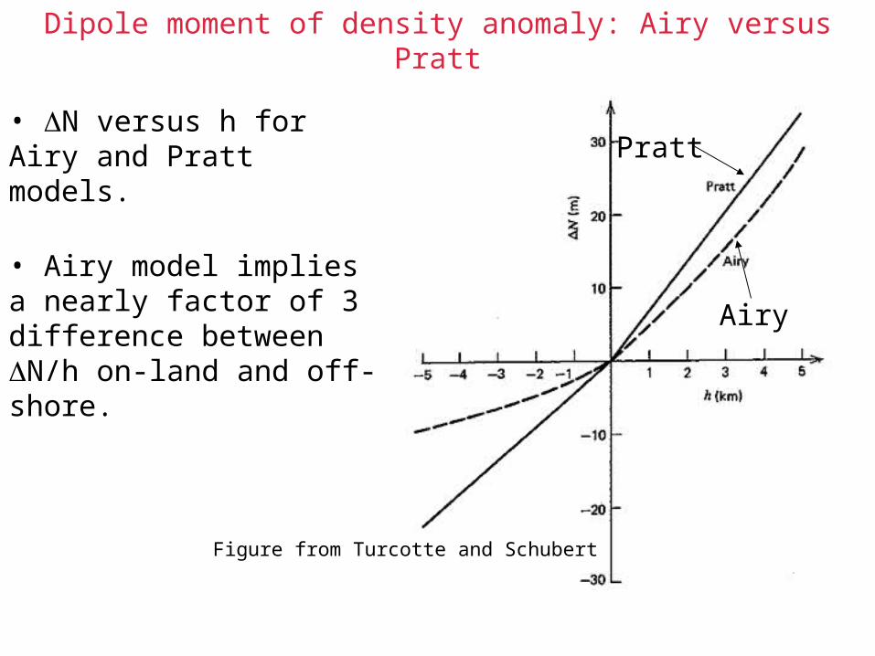
Dipole moment of density anomaly: Airy versus Pratt

Pratt

Airy

• ΔN versus h for Airy and Pratt models.

• Airy model implies a nearly factor of 3 difference between ΔN/h on-land and off-shore.

Figure from Turcotte and Schubert

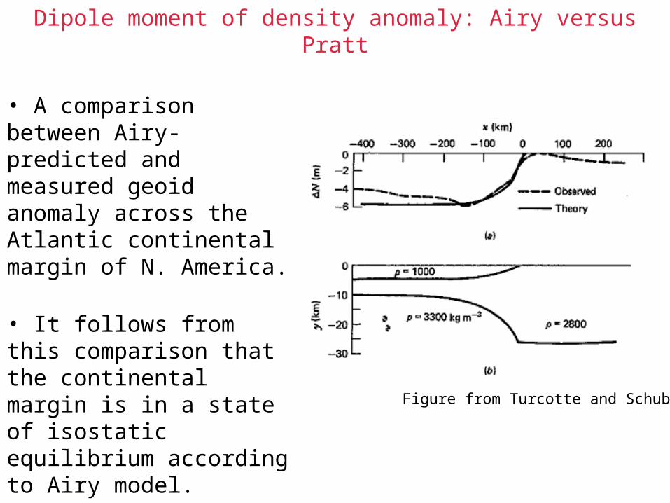
Dipole moment of density anomaly: Airy versus Pratt

• A comparison between Airy-predicted and measured geoid anomaly across the Atlantic continental margin of N. America.

• It follows from this comparison that the continental margin is in a state of isostatic equilibrium according to Airy model. Figure from Turcotte and Schubert

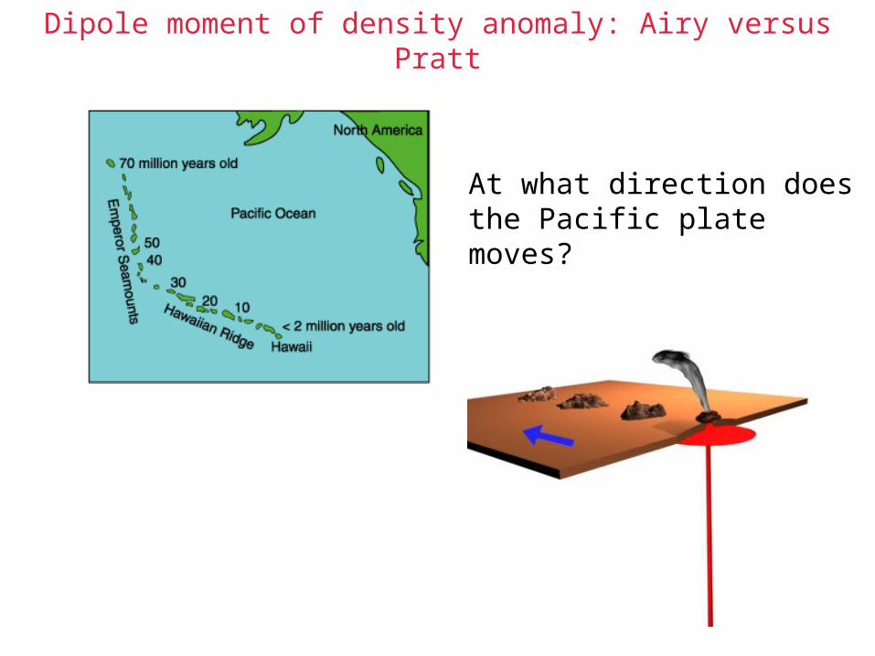
At what direction does the Pacific plate moves?

Dipole moment of density anomaly: Airy versus Pratt

Dipole moment of density anomaly: Airy versus Pratt

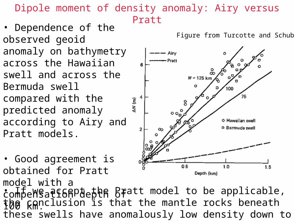
Figure from Turcotte and Schubert• Dependence of the observed geoid anomaly on bathymetry across the Hawaiian swell and across the Bermuda swell compared with the predicted anomaly according to Airy and Pratt models.

• Good agreement is obtained for Pratt model with a compensation depth of 100 km.

• If we accept the Pratt model to be applicable, the conclusion is that the mantle rocks beneath these swells have anomalously low density down to a depth of 100 km.