Embed Size (px)
Citation preview
econstorMake Your Publication Visible
A Service of
zbwLeibniz-InformationszentrumWirtschaftLeibniz Information Centrefor Economics
Baier, Scott L.; Bergstrand, Jeffrey H.; Clance, Matthew W.
Working Paper
Heterogeneous Economic Integration AgreementEffects
CESifo Working Paper, No. 5488
Provided in Cooperation with:Ifo Institute – Leibniz Institute for Economic Research at the University ofMunich
Suggested Citation: Baier, Scott L.; Bergstrand, Jeffrey H.; Clance, Matthew W. (2015) :Heterogeneous Economic Integration Agreement Effects, CESifo Working Paper, No. 5488
This Version is available at:http://hdl.handle.net/10419/123124
Standard-Nutzungsbedingungen:
Die Dokumente auf EconStor dürfen zu eigenen wissenschaftlichenZwecken und zum Privatgebrauch gespeichert und kopiert werden.
Sie dürfen die Dokumente nicht für öffentliche oder kommerzielleZwecke vervielfältigen, öffentlich ausstellen, öffentlich zugänglichmachen, vertreiben oder anderweitig nutzen.
Sofern die Verfasser die Dokumente unter Open-Content-Lizenzen(insbesondere CC-Lizenzen) zur Verfügung gestellt haben sollten,gelten abweichend von diesen Nutzungsbedingungen die in der dortgenannten Lizenz gewährten Nutzungsrechte.
Terms of use:
Documents in EconStor may be saved and copied for yourpersonal and scholarly purposes.
You are not to copy documents for public or commercialpurposes, to exhibit the documents publicly, to make thempublicly available on the internet, or to distribute or otherwiseuse the documents in public.
If the documents have been made available under an OpenContent Licence (especially Creative Commons Licences), youmay exercise further usage rights as specified in the indicatedlicence.
www.econstor.eu
Heterogeneous Economic Integration Agreement Effects
Scott L. Baier Jeffrey H. Bergstrand Matthew W. Clance
CESIFO WORKING PAPER NO. 5488 CATEGORY 8: TRADE POLICY
AUGUST 2015
An electronic version of the paper may be downloaded • from the SSRN website: www.SSRN.com • from the RePEc website: www.RePEc.org
• from the CESifo website: Twww.CESifo-group.org/wp T
ISSN 2364-1428
CESifo Working Paper No. 5488
Heterogeneous Economic Integration Agreement Effects
Abstract Gravity equations have been used for more than 50 years to estimate ex post the partial effects of trade costs on international trade flows, and the well-known - and traditionally presumed exogenous – “trade-cost elasticity” plays a central role in computing general equilibrium trade-flow and welfare effects of trade-cost changes. This paper addresses theoretically and empirically the influence of variable and fixed export costs in explaining the likely heterogeneity in the trade-cost elasticity. We offer four potential contributions. First, for motivation, we show empirically that the heterogeneity in various economic integration agreements’ (EIAs’) partial effects on trade flows far exceeds that explained simply by variation in depth of the trade liberalization. Second, we use standard Armington- and Melitz-type general equilibrium trade models to motivate theoretically the roles of variable trade costs and of fixed and variable export costs, respectively, for explaining (endogenous) heterogeneous partial effects of changes in ad valorem tariff rates on trade flows, as well as on intensive and extensive product margins (with or without network effects and with an untruncated Pareto distribution in the Melitz model). Third, we show empirically that the heterogeneity in EIAs’ partial effects on the intensive margin is explained well just by distance and adjacency, capturing variable natural trade costs; however, the heterogeneity in EIAs’ partial effects on the extensive margin is explained empirically by distance and adjacency, as well as several other cultural and institutional variables, capturing variable and fixed export costs. Fourth, we show that such estimated heterogeneous effects can predict 83-94 percent of economic welfare effects of EIAs and can potentially predict ex ante a potential EIA’s partial trade-flow effect and general equilibrium welfare effect.
JEL-Code: F100, F120, F130, F140, F150.
Keywords: international trade, economic integration agreements, gravity equation.
Scott L. Baier John E. Walker Department of Economics
Clemson University USA – Clemson, SC 29634
[email protected] Jeffrey H. Bergstrand
Mendoza College of Business University of Notre Dame
USA – Notre Dame, IN 46556 [email protected]
Matthew W. Clance Department of Economics
University of Pretoria South Africa – Hatfield 0028
[email protected] August 10, 2015
The welfare eects in this class of model are linked to the change in the share of trade thattakes place inside a country.... Intuitively, because the initial ows are so small, even doubling tradewith ex-colonies will result in very tiny changes in the share of expenditure that is spent locally.In contrast, adding even a few percentage points of trade with a major partner will
be much more important for welfare. (Head and Mayer, Gravity Equations, Handbook ofInternational Economics, vol. 4, 2014; bold added)
1 Introduction
The gravity equation has been used for more than 50 years since Tinbergen (1962) to explain
statistically ex post the cross-sectional and panel variation of bilateral international (aggregate
goods) trade ows and the partial eects of economic integration agreements (EIAs) on such ows.
However, the link between these ex post estimates and the welfare gains from trade liberalization has
been at best tenuous. This paper addresses this shortcoming, picking up to a large extent where
Helpman, Melitz, and Rubinstein (2008) left o. While xed export costs and rm heterogeneity
are now recognized as important to explain intensive margin, extensive margin, and aggregate trade
ow levels, we show that such factors are also important to explain quantitatively the size of partial
eects of EIAs (and, in general, trade liberalizations) on intensive margin, extensive margin and
aggregate trade ow levels and to approximate the (general equilibrium) welfare eects of EIAs.
Typically, the trade ow from one country to another in a gravity equation is explained using
the exporting and importing countries' gross domestic products (GDPs), bilateral distance, and
an array of other explanatory variables, including dummy variables for EIAs. In fact, one focus
of Tinbergen (1962) was to examine the partial eect of preferential trade agreements on trade
ows. While Tinbergen (1962) is typically cited as the rst published gravity-equation study of
trade ows, researchers using the international trade gravity equation have seldom explored some
of the novel contributions and anomalies of this seminal study. For instance, Tinbergen's rst
specications included dummy variables for common membership in the British Commonwealth and
for common membership in the Belgium-Netherlands-Luxembourg (BENELUX) economic union.
Allowing the two agreements to have heterogeneous (partial) eects, Tinbergen found trivial impacts
of these agreements on members' trade. However, in a later specication using a single dummy
for membership in any preferential trade agreement, Tinbergen found that common membership
increased trade for the typical pair bymore than 100 percent. This completely overlooked contrasting
result is just one of several motivations for our paper exploring determinants of the heterogeneity
in EIAs' partial eects.
Of course, hundreds of gravity-equation analyses have been published (and many more com-
pleted) in the last 50 years with thousands of estimates of (like Tinbergen (1962)) the bilateral
trade impacts of common membership in some form of EIA.1 Cipollina and Salvatici (2010) con-
ducted a meta analysis of estimates of the (partial) eects of EIAs on trade ows and found a mean
(median) eect of 0.59 (0.38), implying an increase of 80 (46) percent. The eects range from -9.01
1We use the term economic integration agreement to broadly capture any of one-way or two-way preferential tradeagreements, free trade agreements, customs unions, common markets, or economic unions.
2
to 15.41 including outliers. Once xed or random eects are introduced, the minimum estimate
is 0.01 and the maximum estimate is 1.52. Similarly, Head and Mayer (2014) in a meta analysis
found mean (median) estimates of 0.59 (0.47) and considerable partial eect heterogeneity. The vast
heterogeneity in EIAs' estimated trade-ow eects motivated Anderson and van Wincoop (2004) to
note:
Implausibly strong regularity (common coecients) conditions are often implicitly imposed onthe trade cost function [in gravity equations]. For example, the eect of membership in a customsunion or a monetary union on trade costs is often assumed to be uniform for all members. (p. 711)
This paper has four goals. First, using a random coecients econometric analysis we demonstrate
that not only is there considerable heterogeneity in EIAs' (partial) impacts on trade but the
heterogeneous EIA eects far exceed what can be explained by the degree of trade liberalization of
such agreements. It is well known that every economic integration agreement is unique in terms of
the degree of trade liberalization, e.g., degree of decline in τijt (where τijt is an ad valorem measure
of taris and nontari barriers of country j on country i's goods in year t). However, it is also
well known that empirical ad valorem measures of bilateral tari rates are subject to measurement
error; ad valorem measures of nontari barriers (also lowered by EIAs) are likely worse. Yet the
reduction of nontari barriers has been taking center stage in recent important proposed EIAs, such
as the Transatlantic Trade and Investment Partnership (TTIP), cf., Berden, Francois, Tamminen,
Thelle, and Wymenga (2010) and Francois, Manchin, Norberg, Pindyuk, and Tornberger (2013).
Moreover, as Anderson and van Wincoop (2004) note, Particularly egregious is the paucity of good
data on policy barriers (p. 693).2 Consequently, recent advances in gravity-equation modeling have
turned to panel data methodologies to nd unbiased and precise empirical estimates of the average
treatment eects of EIAs on trade ows to avoid the measurement-error issues associated with
crude estimates of τijt, cf., Baier and Bergstrand (2007), Anderson and Yotov (2011), and Eicher,
Henn, and Papageorgiou (2012). In particular, Baier, Bergstrand, and Feng (2014), or BBF, found
economically plausible, unbiased, and precise estimates of the average treatment eects of one-way
preferential, two-way preferential, free, and deeper trade agreements. In section 2, we extend the
methodology in BBF to show that the heterogeneity in EIAs' partial eects on trade far exceeds
that from the degree of liberalization, suggesting the need to search for other factors to explain
the heterogeneity in EIA (partial) eects. Preliminary empirical evidence from Baier, Bergstrand,
and Clance (2015) suggests that EIA dummies' coecient estimates are systematically related to
various observable bilateral trade-cost proxies.
Second, motivated by the empirical random coecients analysis, we use Armington- and Melitz-
type general equilibrium models to explain theoretically why trade-cost elasticities are likely endoge-
nous and related to the levels of country-pairs' variable export costs and xed and variable export
costs, respectively (and do not necessarily depend on externalities or the underlying distribution
2See Anderson and van Wincoop (2004), section 2 for a poignant and thorough description of the inadequacy ofdata on taris and non-tari measures for trade economists.
3
of productivities in the Melitz model). Only four recent studies (to the authors' knowledge) have
argued that trade-cost elasticities are theoretically endogenous. Helpman, Melitz, and Rubinstein
(2008), or HMR, was the rst to generate a rationale for heterogeneous trade impacts of a given
percent change in trade costs using constant elasticity of substitution (CES) utility. With heteroge-
neous rms, HMR argued that a given percent change in trade costs would cause some countries to
start trading (via the extensive margin); the trade-cost elasticity becomes endogenous to the specic
country-pair ij as determined by the probability of positive exports for pair ij (ρij). Their empirical
exercise showed that the distance elasticity varied and tended to decrease (in absolute terms) with
the per capita income of the country-pair; however, they did not explore the explicit relationship of
this heterogeneity to variable trade costs relative to xed trade costs, nor xed policy trade costs rel-
ative to xed non-policy trade costs. Krautheim (2012) picked up on the relevance of the extensive
margin with CES preferences for inuencing the trade-cost elasticity by introducing network eects.
In his baseline model, network eects (spillovers) magnify the trade-cost elasticity, but do not en-
dogenize it. In his paper's last section, consideration of an additively separable xed export cost
potentially endogenizes his trade-cost elasticity; however, he does not derive closed-form solutions
for the endogenous trade-cost-elasticity case. More recently, Melitz and Redding (2015) detailed
the importance of small deviations from the parameter restrictions in Arkolakis, Costinot, and
Rodriguez-Clare (2012), or ACR, to demonstrate that trade-cost elasticities are potentially endoge-
nous. In particular, Melitz and Redding (2015) show that a simple distinction between untruncated
and truncated Pareto productivity distributions can cause the dierence between exogenous and en-
dogenous trade-cost elasticities. With a truncated Pareto productivity distribution, the trade-cost
elasticity is sensitive to the share of exporters in the domestic market (and the cuto productivity),
a function of the specic country-pair's xed export costs; in the case of an untruncated Pareto
distribution, their trade-cost elasticity is exogenous. While all three papers focus on extensive mar-
gin eects for endogenizing the trade-cost elasticity, all maintain the intensive-margin trade-cost
elasticity to be constant (under CES preferences). Only Novy (2013) conjectured theoretically an
endogenous trade-cost elasticity by assuming (non-CES) transcendental logarithmic (or translog)
preferences; however, his empirical work used aggregate trade ows, rather than intensive margins,
for evidence.
This paper extends this literature theoretically. In section 3, we show in the context of a simple
Armington model with constant-elasticity-of-substitution preferences how tari removals' eects on
trade (at the intensive margin) that is, the trade-cost elasticity can be sensitive to the levels of
ad valorem bilateral variable export costs between two countries by assuming the more empirically
plausible trade-cost function of Hummels and Skiba (2004) and Anderson and van Wincoop (2004).
In section 4, we extend the Melitz-type model in Krautheim (2012) to motivate how the interactions
of exogenous factors inuencing xed export costs (such as bilateral distance as well as bilateral
dummy variables capturing institutional (policy) and cultural (non-policy) characteristics) with en-
dogenous xed export costs associated with network eects can additionally explain theoretically
the sensitivity of the elasticity of the extensive margin of trade ows with respect to variable tari
rate levels and with respect to xed export costs (even with an untruncated Pareto productivity
4
distribution). We derive novel closed-form solutions for the relationships between (additively sep-
arable) exogenous xed export costs, endogenous network xed export costs, productivity cutos,
and extensive margins of trade with CES preferences and for the relationships between policy-based
xed export costs, non-policy based xed export costs, productivity cutos, and extensive margins
of trade.
Third, guided by these theoretical results, we show empirically that the heterogeneity in EIAs'
eects can be explained well by (exogenous) observable factors commonly used to explain these vari-
able and xed export costs. In section 5, we use our theory to motivate the relationships between
HMR's geographic, institutional, and cultural variables and the variation in EIAs' eects on the
intensive and extensive margins. Specically, we show that distance and adjacency inuencing
variable transport costs explain well the heterogeneity in EIA partial eects on the intensive (prod-
uct) margin. Moreover, distance, adjacency, and typical gravity dummy variables reecting common
institutional and cultural country characteristics capturing (policy and non-policy, respectively)
xed export costs explain well the heterogeneity in EIA partial eects on the extensive (product)
margin. To the best of our knowledge, only two studies have estimated heterogeneous EIA eects
using interaction terms like here to avoid the dilemma of a multitude of individual dummies that
yield econometrically weak coecient estimates. Vicard (2011) investigated empirically interactions
of numerous economic variables with EIA dummies, but the study was not guided by theory and
so interaction eects lacked economic interpretation. Cheong, Kwak, and Tang (2015) examined
empirically interactions of EIA dummies with measures of GDP size and similarity and found signif-
icant eects, but this study also lacked theoretical guidance. Also, both of those studies looked only
at aggregate trade ows. Our study is unique by oering theoretical guidance from Armington and
Melitz models to understand the roles of variable trade costs and of xed and variable export costs,
respectively with or without network externalities and with an untruncated Pareto distribution
for explaining heterogeneous EIA eects, for explaining dierential EIA eects quantitatively and
qualitatively on intensive and extensive (product) margins, and for controlling for various degrees
of EIA liberalization (as raised in Kohl, Brakman, and Garretsen (2014)).3
Since our theory suggests that EIAs' eects may be inuenced by factors inuencing both the in-
tensive and extensive margins of trade, Section 6 employs the Hummels and Klenow (2005) product-
margin-decomposition methodology to explore empirically how distance and other factors inuence
such margins' EIA eects. We show that various factors inuence EIAs' eects on intensive and
extensive margins of trade dierently, quantitatively and qualitatively. This section also provides a
robustness analysis of our main results to lagged terms-of-trade eects, nontradable goods' cutos,
and interaction eects by type of EIA.4
3We intentionally use an untruncated Pareto distribution for productivities to distinguish the economic channelsexplaining our endogenous trade-cost elasticities from those channels addressed in Melitz and Redding (2015).
4It is important to note that, although we focus on heterogeneous partial eects of EIA dummies, our analysisholds in principle for ad valorem tari rates as well, such as in Baier and Bergstrand (2001). Our focus empiricallyon heterogeneous EIA dummy coecients, rather than heterogeneous tari-rate elasticities, is due to the paucityof high quality ad valorem tari-rate (and nontari-rate) data and the empirical prominence of EIA dummies in theliterature. Nevertheless, our theory will be cast with a focus on heterogeneous partial tari-rate elasticities. We leavefor future research applying the methodology in this paper to the case where high quality ad valorem measures ofbilateral tari and nontari barriers are available.
5
Fourth, we address directly our introductory quote and show that the our approach to gravity-
equation modeling now makes more plausible ex ante use of gravity equations for predicting the
partial eects of future EIAs and their likely welfare eects. Studies such as Baier and Bergstrand
(2007), or BB, and BBF can help policymakers predict future partial (and then general) equilibrium
eects of a planned EIA; BB (BBF) predicts the average eect without (with) regard to type of
EIA. However, those predicted partial eect estimates are homogeneous across country-pairs (based
on average treatment eects). In section 7, we show that estimating quantitatively the sensitivity
of estimated partial eects to geographic, institutional, and cultural characteristics enables gravity
equations to more precisely inform policy makers ex ante of pair-specic predicted impacts of EIAs
accounting for both heterogeneous general and partial equilibrium eects. We will show that the
heterogeneity of EIA partial eects helps to explain the likely welfare gains and predictability of
EIAs, as well as the timing of EIAs. For instance, we will show that 83-94 percent of the welfare
gain for country j of an EIA with country i can be explained by the heterogeneous partial trade
elasticity along with the share of country j's imports from country i, consistent with the introductory
quote. Put succinctly, previous gravity equations allowing for heterogeneous partial eects of EIAs
on trade have been limited not just by weak estimates (to be discussed shortly), but allowed only
ex post evaluation. Our paper suggests a methodology for generating robust and precise partial
eect estimates that can also be used potentially for ex ante trade and welfare analysis, which
we demonstrate in Section 8 for the the proposed Transatlantic Trade and Investment Partnership
(TTIP).5 Section 9 provides conclusions.
2 Empirical Motivation for the Theory
In this section, we demonstrate that there is considerable heterogeneity in the (partial) eects of
EIAs, independent of the depth of the EIA, using a random coecients econometric approach.
First, we address econometrically how the most recent panel approach to estimate gravity can be
extended to allow for random coecient estimates to illustrate the large heterogeneity of EIA eects
even after accounting for the depth of EIA. The second section discusses the data and presents
the results.
2.1 Heterogeneous Partial EIA Eects
Most of the trade-policy liberalizations in the past 25 years have been bilateral (and plurilateral)
EIAs, such as free trade agreements. However, typically EIAs are broad agreements reaching beyond
elimination of ad valorem tari rates (which are variable trade costs). They have also lowered
xed export costs.6 For instance, see Horn, Mavroidis, and Sapir (2010) on the numerous non-
5It should also be noted that traditional ex ante computable general equilibrium models typically use trade-costelasticities previously estimated from empirical specications assuming homogeneous average partial eects. We alsoaddress in section 7 that our heterogeneous trade-cost elasticities violate macro restriction R3 in Arkolakis, Costinot,and Rodriguez-Clare (2012) so that welfare cannot be measured solely by the share of domestic output absorbeddomestically and an exogenous trade-cost elasticity.
6Consequently, later in the paper, we will distinguish bilateral xed export costs associated with policy, denotedFXPijt , from bilateral xed export costs associated with non-policy, or natural, factors, denoted FXNijt .
6
tari-rate provisions covered in an anatomy of European Union and United States' preferential
trade agreements. Thus, EIA liberalizations likely lower τijt and FXPijt . Moreover, as noted in the
introduction, empirical ad valorem measures of bilateral tari rates are subject to measurement
error; ad valorem-equivalent measures of nontari barriers (also lowered by EIAs) are worse. This
measurement issue further complicates estimation of the trade-cost elasticity.
Consequently, researchers using gravity equations have turned instead to panel data methodolo-
gies with dummy variables to nd unbiased and precise empirical estimates of the average treatment
eects of EIAs on trade ows, cf., BB, Anderson and Yotov (2011), Eicher, Henn, and Papageorgiou
(2012), and Head and Mayer (2014). For instance, BB showed that unbiased and precise estimates
of EIAs on bilateral trade ows could be captured using the gravity-equation specication below
using ordinary least squares (OLS):7
lnXijt = α+ ηit + θjt + ψij + βEIAijt + υijt (1)
where ηit is an exporter-year xed eect, θjt is an importer-year xed eect, ψij is a country-pair
xed eect, and υijt is an error term. Equation (1) is commonly referred to as a xed eects
model. However, it will be useful now to emphasize as well that this is also a xed parameters
model (i.e., β is a xed parameter). Hence, BB was a xed eects, xed parameter model, and that
is also the case to the best of our knowledge for virtually all like gravity analyses. A key insight
of BB was to show methodologically and empirically the importance of the country-pair xed eect
for controlling for the endogeneity of the EIA variable.
As noted earlier in the quote from Anderson and vanWincoop (2004), a limitation of equation (1)
is that it imposes a common estimated average partial eect for all EIAs; EIAs and their eects on
trade ows are likely to be heterogeneous. In specications such as equation (1), this heterogeneity
in EIAs' partial eects is captured in the error term, υijt, which is assumed to be uncorrelated with
the other right-hand-side (RHS) variables.
Three issues arise when considering the potentially heterogeneous eects of EIA dummies. One
issue is that a single EIA dummy cannot capture the heterogeneity among EIAs in their degrees
of trade liberalization, cf., the quote in the introduction by Anderson and van Wincoop (2004).
Historically, several studies have attempted to allow for (ex post) heterogeneous EIA eects by
introducing instead a multitude of dummies one for each agreement. However, this approach
often leads to weak estimates. The reason is that unless the EIA is plurilateral with numerous
common memberships there is insucient variation in the RHS dummy variables. This was the
dilemma Tinbergen (1962) faced, leading to the trivial EIA eects of the British Commonwealth
and BENELUX economic union.8 Second, even within a plurilateral agreement, it is possible that
the bilateral eect of a common EIA diers owing to variance in geographic, institutional, and
cultural factors, ignored in in typical gravity estimates. Third, as will be discussed more later, even
if individual EIA dummies' partial eect could be estimated with precision and consistency, they
7For now, we ignore zero trade ows, allowing a log-linear gravity equation. See BB and BBF for theoreticalgravity-equation motivation for equation (1).
8There were only three countries in each agreement in his sample and only six 1's in each of the dummy variables.
7
remain only ex post estimates.
Among several issues addressed, BBF dealt with the rst issue avoiding weak estimates as-
sociated with a multitude of dummies by running a specication including separate dummies
for one-way PTAs (OWPTA), two-way PTAs (TWPTA), FTAs, and a dummy combining customs
unions, common markets, and economic unions (CUCMECU), due to the limited number of these
more integrated EIAs in their sample ending in 2005.9 Hence, BBF ran the xed eects, xed
parameters model:
lnXijt = α+ ηit + θjt + ψij + β1OWPTAijt + β2TWPTAijt + β3FTAijt
+β4CUCMECUijt + υijt (2)
using OLS.10 Among other ndings, BBF found that deeper economic integration agreements had,
as expected, larger partial eects on bilateral trade ows.
A second issue is that the partial eect on trade of EIAs with a given degree of trade liberalization
may be heterogeneous due to variable and/or xed bilateral export costs. For tractability, suppose
EIAijt represents EIAs with a given degree of trade liberalization. Following Cameron and Trivedi
(2005) (p. 774), we can consider the specication:
lnXijt = α+ ηit + θjt + ψij + βijEIAijt + υijt (3)
where the partial eect of an EIA on lnXijt is allowed to be pair-specic. One way to interpret the
heterogeneity in the βij 's is to assume it is random. For instance, assume βij = β + bij where bij is
a zero mean random variable. In this case, the expectation of βij is:
E(βij | ηit, θjt, ψij , EIAijt) = β
In section 2.2 below, we make this assumption to illustrate the enormous heterogeneity in values
of βij , even after accounting for dierent degrees of trade liberalization. We will refer to these
regressions as the random coecients models.
Alternatively, suppose there exists a set of variables Zij such that:
E(lnXijt | α, ηit, θjt, ψij , βij , EIAijt, Zij) = α+ ηit + θjt + ψij + βijEIAijt (4)
9In this paper, we have extended that data set to 2011, enlarging substantially the number of EIAs with customsunions (CUs), common markets (CMs), and economic unions (ECUs), and so will treat each of those types separately.
10Ignoring zeros could potentially bias results, due to country selection; moreover, one must account for potentialbias due to rm heterogeneity in aggregate data, cf., Helpman, Melitz, and Rubinstein (2008). However, BBF showedthat potential bias due to country selection and rm heterogeneity was largely cross sectional in nature and couldbe accounted for in panel data by the pair xed eects; see BBF and its Online Theoretical Supplement for acomprehensive discussion. Also, due to potential heteroskedasticity owing to Jensen's inequality, some studies haveemployed Poisson Quasi-Maximum Likelihood (PQML). Due to our specication using a very large number of xedeects, researchers have only been able to obtain convergence under PQML for a limited time series in the panel (i.e.,a short panel), cf., Bergstrand, Larch, and Yotov (2015). Consequently, due to our long panel, this limitation allowsus to only use OLS. We also note that Bergstrand, Larch, and Yotov (2015) found, if anything, that OLS biaseddownward the EIA partial eect estimates relative to PQML estimates.
8
Without knowing the true values of the βij , we take expectations over all variables to obtain:
E(lnXijt | α, ηit, θjt, ψij , EIAijt, Zij) = α+ ηit + θjt + ψij
+E(βij | α, ηit, θjt, ψij , EIAijt, Zij)EIAijt
We assume that the expected eect of an EIA between i and j, conditioning on all other variables,
is given by:
E(βij | ηit, θjt, ψij , Zij) = β + bZ(Zij − µZ)
where Zij − µZ denotes the de-meaned values of Zij . Absent knowledge of βij , following Cameron
and Trivedi (2005) we should estimate instead:
E(lnXijt | α, ηit, θjt, ψij , EIAijt, Zij) = α+ ηit + θjt + ψij + βEIAijt + bZ(Zij − µZ)EIAijt (5)
One of the main goals of this paper is to identify the variables in Zij to determine the best linear
unbiased predictors. In fact, Sections 3 and 4 below will rst motivate theoretically in the context
of Armington and Melitz models the roles of bilateral variable trade costs and of bilateral xed
and variable export costs, respectively, in explaining the heterogeneous βij we nd empirically in
Section 6.
A third issue is that previous estimates of EIA partial eects have been ex post. As mentioned
at the paper's outset, the link between estimated ex post gravity EIA partial eects and the ex ante
welfare eects of a trade liberalization has been at best tenuous. In this paper, our identication
of the geographic, institutional and cultural factors that explain heterogeneous EIA partial eects
βij can be used potentially for predicting ex ante the partial trade eect of a specic country-pair's
EIA. In the spirit of the sucient statistics approach in ACR, we show specically that the ex ante
change in welfare in importing country j from an EIA with exporting country i can be represented
by the product of βij (using estimates of bZ), the share of i's exports in j's aggregate expenditures
(λij), the CES utility parameter, and an error term capturing general equilibrium inuences. Later,
we will show empirically that data only on λij and estimates of βij can explain between 83-94
percent of the welfare gains for an importing country of an EIA, and thus potentially can be used
for ex ante welfare predictions.
However, before we proceed to exploring potential sources of Zij , it would be useful rst just
to get a sense of how large the potential heterogeneity of βij might be even without knowing the
source (i.e., the Zij). Consequently, to illustrate how large the heterogeneity of βij might be, we
will estimate equation (3) allowing for all six dierent types of EIAs using the random coecients
approach. Estimation of equation (3) will account for the heterogeneity in dierent degrees of trade
liberalization; however, without controlling at this stage for the Zij−µZ , we anticipate bias in thesepreliminary (motivating) random coecient estimation results.11
11One further consideration is noteworthy. Since gravity equations typically use binary variables to capture thepolicy change rather than an ad valorem variable such as τijt, the dummy variable's coecient estimate is a combi-
9
2.2 Data and Results
Nominal trade ows are from the United Nations' COMTRADE database for the years 1965, 1970,
1975, 1980, 1985, 1990, 1995, 2000, 2005 and 2010. Bilateral distances, adjacency, common language,
religion similarity, common legal origin, and common colonial history (used later) are from the BACI
data set. The data set for EIAs comes from Baier and Bergstrand's data set for 2014.12 There are
183 countries included in our data set. Online Appendix 1 lists the EIAs in our sample and (at its
end) the countries included.
Table 1 provides a decomposition of the data set into types of agreements. Note that the
vast majority of observations have no economic integration agreement and less than 6 percent of
the observations have FTAs, CUs, CMs, or ECUs. In Table 1, the subtotal of 726,468 observations
indicates the total number of annual positive trade ow observations for 49 years from 1962-2010 for
the 33,306 country-pairs; the missing observations are composed largely of zeros.13 As discussed
in BB and BBF, we only use observations from every ve years. The primary reason is that Cheng
and Wall (2005) and Wooldridge (2000) both argue in favor of using data drawn from a period
longer than annually. For instance, Cheng and Wall (2005) note that Fixed-eects estimations are
sometimes criticized when applied to data pooled over consecutive years on the the grounds that
dependent and independent variables cannot fully adjust in a singe year's time (p. 8; italics added).
A second reason is that the number of xed eects related to equation (3) or (4) with potentially
33,306 (directional) bilateral trade ows and 49 years, or 1,631,994 potential observations (or even
726,468), is only computable in STATA using higher dimension xed eects; restricting the data
to every ve years from 1965-2010 reduces the number of xed eects to a manageable level for
estimation without such techniques. Consequently, our potential number of observations, based on
positive trade ows, is 155,718.
Table 2 presents several sets of results. Since this is the rst paper to also provide separate
partial eects for all six EIA categories in the Baier-Bergstrand EIA Database, before providing the
results from the random coecients specication we provide the results rst for various versions of
xed eects, xed parameters equations (1) and (2), where equation (2) is modied to include six
dummy variables. Table 2 has ten columns, reporting the results of eight dierent specications of
equations (1) and (2). Column (1) provides the names of alternative groupings of EIAs. Column 2
provides the expected coecient sign. The rst three specications in columns (3)-(5) are similar
to equation (1), with no lags and combining dierent EIA types into one or two dummy variables;
t-statistics are in parentheses. The fourth specication in column (6) is similar to equation (2). The
last four specications in columns (7)-(10) include additionally a ve-year lag of each RHS variable.
nation of ε and −ρ, where −ρ is an estimate of the eect of the EIA's formation on lowering τijt. For this study, wewill use the dierences in partial eects across types of EIAs to gain insight about −ρ. For example, the dierencein BBF between a deeper EIA and a one-way PTA (e.g., Generalized System of Preferences agreement) is 0.295(=0.696-0.401). For a common ε, this dierence informs us of the relative change of τ between the two types ofagreements.
12See www.nd.edu/ jbergstr. The version we use is a cleaned and extended-to-2011 version of the May 2013 dataset; it is available on request.
13Recall our earlier footnote on why our results will not be subject to selection or rm-heterogeneity bias, followingmethodology used in BBF.
10
Previous studies such as BB and BBF have shown that, due to phase-ins of agreements as well as
lagged eects of EIAs on terms-of-trade, EIA dummies tend to have lagged eects on trade ows.
Specication 1 in column 3 uses a conventional grouping of EIAs: free trade agreements (FTAs,
or 3), customs unions (CUs, or 4), common markets (CMs, or 5) and economic unions (ECUs, or 6).
We denote this grouping EIA3-6, which reects the inclusion of EIAs of levels 3-6. The coecient
estimate of 0.56 is very similar to the partial eect estimated in BB; it implies the typical EIA
using categories 3-6 increases trade (absent any general equilibrium eects) by approximately 90
percent. This coecient estimate of 0.56 is very similar also to the mean estimate of 0.59 in the
meta analyses in both Cipollina and Salvatici (2010) and Head and Mayer (2014).
Specication 2 in column 4 adds another EIA dummy to capture the eects of preferential
trade agreements (PTAs). In the Baier-Bergstrand EIA database, a 1 denotes a one-way PTA
(OWPTA), including Generalized System of Preferences (GSP) agreements. A 2 denotes a two-way
preferential trade agreement (TWPTA), where there are preferences extended but it is not an FTA.
In Specication 2, we include EIA1-2 as well as EIA3-6; EIA1-2 denotes a one if two countries
have a one-way or two-way PTA. Not surprisingly, the coecient estimate for EIA1-2, 0.096, is
considerably smaller than that for EIA3-6; there is less liberalization typically in agreements in
EIA1-2.
Specication 3 in column 5 uses EIA1-6, all six levels of EIAs. Not surprisingly, the partial
eect is roughly half of that for EIA3-6 in column 3 and roughly halfway between the coecient
estimates in column 4.
Specication 4 in column 6 includes six dummies, one for each of the six types of EIAs in the
Baier-Bergstrand EIA data set, which now has observations through 2011. The coecient estimates
tend to reect the increasing order of perceived trade liberalizations underlying each type of EIA.
The statistically insignicant partial eect of 0.02 for one-way PTAs (EIA1) is consistent with other
studies examining such agreements' trade eects. The coecient estimate of 0.25 for two-way PTAs
is statistically signicant. The statistically signicant FTA coecient estimate of 0.53 accords with
other studies for FTAs. The statistically signicant customs union coecient estimate of 0.84 implies
that such existing agreements tend to have deeper integration than FTAs. Common markets are
expected to be even more integrated than FTAs and CUs, so the statistically signicant coecient
estimate of 1.12 for EIA5 (CMs) is consistent with this notion. Finally, economic unions tend to be
more integrated than common markets, but are dierentiated more along the lines of coordinated
monetary and/or scal policies than deeper integration in trade. Consequently, the slightly lower
coecient estimate for ECUs of 1.032 is plausible in light of the estimate for the common market's
coecient. However, the coecient estimates for CM and ECU are not statistically dierent from
each other.14 Clearly, a considerable portion of the heterogeneity of partial eects of EIAs is
explained by varying degrees of trade liberalization.
The specications in columns 7-10 in Table 2 are analogous to the specications in columns 3-6
except for including additionally a ve-year lag of the EIA. We will not go through these results
14Once lagged EIA eects are included, the total EIA coecient estimates for common markets and economicunions are nearly identical.
11
in detail, as the outcomes conform to those in earlier studies such as BB and BBF, whereby EIAs
have lagged eects on trade ows due to phasing-in of agreements and lagged terms-of-trade eects.
None of the results in Table 2's specications 7-10 are inconsistent with expectations. Note that
the total EIA eect for common markets is 1.16 whereas that for economic unions is 1.17.
We now turn to the results of estimating a modication of equation (3), described in equation
(6) below:
lnXijt = α+ ηit + θjt + ψij + β1ijOWPTAijt + β2ijTWPTAijt + β3ijFTAijt
+β4ijCUijt + β5ijCMijt + β6ijECUijt + υijt (6)
Because of the enormous number of heterogeneous partial eects, we cannot use traditional reporting
in the form of a table. For tractability, the results are presented in graphical form. For brevity, we
present the results for the four most interesting types of EIAs: FTAs, CUs, CMs, and ECUs. For
each type of EIA, we ordered coecient estimates from lowest value to highest value and constructed
the kernel density plots to visualize the range of coecient estimates. For instance, for FTAs there
are approximately 2,500 coecient estimates β3ij . For each of CUs, CMs, and ECUs, there are
smaller numbers of coecient estimates, as there are fewer numbers of such types of EIAs.
Figure 1 provides the results from the random coecients model estimation. We note several
distinguishing features of the results. The rst important conclusion from these results is that
there is considerable heterogeneity in the (partial) eects of EIAs on trade ows. Second, the
heterogeneity in EIA eects cannot be explained solely by the depth of liberalization. FTAs have
an average partial EIA eect of 0.33, CUs have an average eect of 0.92, CMs have an average
eect of 0.91, and ECUs have an average eect of 1.08. Note that these estimates vary from the
corresponding EIAs' partial eects in Table 2. As noted in Section 2.1, this is to be expected;
without the inclusion of the Zij −µZ in the regressions, the estimated partial eects in the random
coecients regressions are expected to be biased. Thus, while there is heterogeneity in the EIA
eects across EIA types, there remains considerable heterogeneity across EIAs even within each
type of agreement. As shown below in Sections 3 and 4, the standard quantitative trade models that
dominate the theoretical international trade literature of determinants of bilateral trade in such
papers as Baier and Bergstrand (2001), Eaton and Kortum (2002), Anderson and van Wincoop
(2003), and Chaney (2008) do not predict heterogeneous partial eects; the partial trade-cost
elasticity is a parameter. Consequently, these preliminary empirical results call rst for extending
the theoretical foundations for the gravity equation to determine factors that might explain such
heterogeneous partial EIA eects (independent of and complementary to issues raised in Melitz and
Redding (2015)).
12
3 A Simple Armington Trade Model with Only Variable Trade
Costs
Duty is not assessed on CIF charges. Customs and Border Protection (CBP) value is determinedbased on the "Price Paid" or "Payable" for the goods, which is usually on the bill of sale or invoiceand bill of lading as the Freight On Board (FOB) price. (U.S. Customs and Border Protection website, 2015)
One of the persuasive aspects of ACR was rst demonstrating their main results in the simplest
possible framework: an Armington trade model. The purpose of this section is to illustrate similarly
in a simple Armington trade model how the elasticity of bilateral trade between a country-pair with
respect to ad valorem taris the trade-cost elasticity (1 − σ, in the Armington model) can be
sensitive to the amount of distance between the country-pair.
First, in a seminal article using the Armington model, Anderson and van Wincoop (2003) show
that the three assumptions of (i) an N -country endowment economy where each country produces
a dierentiated good, (ii) consumers have identical constant-elasticity-of-substitution (CES) prefer-
ences, and (iii) market-clearing yield a gravity equation:
Xij =YiYjYW
τ1−σij
Π1−σi P 1−σ
j
, where Π1−σi =
N∑j=1
YjYW
τ1−σij
P 1−σj
, P 1−σj =
N∑i=1
YiYW
τ1−σij
Π1−σi
, (7)
where Xij is the nominal trade ow from country i to country j, Yi (Yj) is the nominal GDP in i
(j), YW is world GDP, τij is ad valorem gross trade costs (including taris and transportation costs)
on goods exported from i to j (τij > 1), σ is the elasticity of substitution in consumption, and:
Pj =
[N∑i=1
(piτij)1−σ
]1/(1−σ)
(8)
where pi is exporter i's Freight-On-Board (FOB) price of its dierentiated product.
Second, following Hummels and Skiba (2004), we assume the price of a good produced in country
i facing importer j, pij , depends on the exporter's FOB price, pi, and a two-part trade cost that
includes both an ad valorem gross tari rate, tij > 1, and per unit shipping costs, freightij :
pij = pitij + freightij (9)
Note that, consistent with the quote above, tari duties are applied to the FOB price. Equation
(9) can be rewritten as:
pij = piτij = pi(tij + fij) (10)
where fij > 0 is the ad valorem-equivalent of freight charges (fij = freightij/pi). See Hummels and
Skiba (2004) for empirical support for this specication. Substituting equation (10) into equations
13
(7) and (8) yields:
Xij =YiYjYW
(tij + fij)1−σ
Π1−σi P 1−σ
j
(11)
which is analogous to equation (18) in Anderson and van Wincoop (2004, p. 715), ignoring for
brevity the z terms in their paper (which are not important here).
Third, taking the logarithm of equation (11) and dierentiating lnXij with respect to ln tij
yields the trade-cost elasticity for the bilateral tari rate:
d lnXij/d ln tij =1
(fij/tij) + 1(1− σ) (12)
Consequently, in light of the additive relationship between fij and tij in equations (10) and (11), the
trade-cost elasticity for tari rates is no longer exogenous, as in all the so-called quantitative trade
models noted earlier; it is sensitive to fij . Moreover, as well established in Hummels and Skiba
(2004) and Hummels (2007), ad valorem bilateral freight costs fij are highly positively correlated
with bilateral distances. Hence, (in absolute terms) the elasticity of bilateral imports with respect
to ad valorem tari rates is a negative function of bilateral distance. Since EIAs reduce tari
rates, this suggests the hypothesis that the elasticity of (the intensive margin of) trade ows with
respect to EIAij may be negatively related to bilateral distance (and perhaps other bilateral trade
impediments).
4 A Melitz-Type Model with Variable and Fixed Export Costs and
Endogenous Network Eects
The previous simple Armington trade model establishes that the elasticity of trade with respect
to EIAs may be heterogeneous (and endogenous) depending upon bilateral distance and possibly
other bilateral trade impediments. However, the simple Armington model allows only for variable
trade costs and changes in trade on the intensive margin. In this section, we provide a more general
model that also includes policy and non-policy xed export costs, rm heterogeneity, and endogenous
network eects. We show how the elasticity of the extensive margin of trade with respect to tari
rates may also be sensitive to variable and xed export costs. Moreover, we show that the elasticity
of the extensive margin of trade with respect to policy-oriented xed export costs may be sensitive
to various economic factors.
4.1 The Theoretical Model
Our theoretical model picks up where Krautheim (2012) left o in two novel features. First,
we account explicitly for exogenous xed export costs independent of and in addition to network
spillovers. Second, we distinguish between exogenous policy-oriented and non-policy-oriented xed
export costs.
14
The main contribution of Krautheim (2012) was to develop a baseline Melitz-type model where
export xed costs are endogenous and a function of the (endogenous) number of exporters from
country i to country j in the representative industry (his sections 1-3). As Krautheim noted, the
great advantage of his (baseline) model was to obtain a closed-form solution. In his nal section
4, he notes, It is quite likely, however, that in reality some xed costs are entirely (or at least
mainly) independent of the number of exporters (p. 33; italics added) and these independent and
exogenous xed costs may inuence the elasticity of export xed costs with respect to the number of
exporters. However, he does not provide a closed-form general equilibrium model of these inuences
in his paper; this is the purpose of this section (and Online Appendix 2). Moreover, he concludes
his last substantive section of the paper suggesting future empirical work should investigate the
variability of trade-cost elasticities to changes in these exogenous (spillover-insensitive) xed export
cost determinants. Such empirical work is another potential contribution of our paper.
Our theoretical model solves for the closed-form solutions and structural gravity equation of
this Melitz-type model allowing for exogenous policy and non-policy xed export costs (linearly)
independent of the endogenous (network-spillover-based) xed export costs.15 We assume a world
economy with N countries and let Lj denote the (internationally immobile) population and labor
force in country j. We assume a single aggregate industry with heterogeneous rms each producing
dierentiated products under increasing returns to scale.
Consumers (workers) are identical and have the utility function:
U =
(∫ω∈Ω
q(ω)σ−1σ dω
) σσ−1
(13)
where q(ω) denotes the quantity consumed of product ω from the set of varieties Ω available and
σ is the elasticity of substitution in consumption across varieties (σ > 1). Consumers maximize
utility subject to a standard income constraint yielding a demand function in country j for variety
ω imported from country i:
qij(ω) =
(pij(ω)
Pj
)−σ (wjLjPj
)(14)
where Pj = [∫ω∈Ω p(ω)1−σdω]
11−σ , wj is the wage rate in country j, and hence wjLj is aggregate
income in country j.
Firms in country i are assumed to have heterogeneous productivities. Potential entrants face
a xed entry cost, FEi . In order to sell in a foreign market j, a rm has to pay an additional
xed export cost, FXij .16 We assume furthermore that xed export costs FXij can be decomposed
linearly into xed costs associated with what we term natural (or non-policy) impediments
into markets (such as costs associated with geographic distance or cultural dierences), FXNij , and
15Online Appendix 2 provides a non-trivial extension of Krautheim's baseline model to include additively separableexogenous and endogenous export xed costs, and provides closed form solutions to a general equilibrium model withlabor-market clearing and free entry and exit of rms. Moreover, at the end of this appendix, we demonstrate formallythe mathematical diculty of combining our trade-cost function in Section 3 with the Melitz model in Section 4 intoone tractable model.
16Krautheim (2012) uses instead Cij to denote these xed costs.
15
xed export costs associated with the destination market's trade policy impediments (such as
regulatory costs associated with institutional dierences), FXPij . We assume that the costs for a
rm (c) with productivity ϕ in country i to sell qij units of output in country j facing (gross) ad
valorem iceberg variable trade costs τij (hence, assuming τij ≥ 1) is given by:
c(qij) =wiqijτijϕ
+ wj(FXNij + FXPij ) (15)
Facing demand curve equation (14), the price charged in j by a rm in i is given by:
pij(ϕ) =wiτijρϕ
(16)
where ρ = (σ − 1)/σ.
Up to now, our economy is characterized by a standard Melitz model, except for distinguishing
two types of export xed costs (policy and non-policy). Following Krautheim (2012), we introduce
network eects into the natural xed export costs (FXNij ). Distinct from the baseline model
in Krautheim (2012), we assume that natural xed export costs are determined by an exogenous
component (AXNij ) and an endogenous component reecting network eects (n−ηij ). We note now
that we will demonstrate that the presence of exogenous xed export component AXNij can inuence
the eect of an EIA with or without network spillovers; moreover, network spillovers can inuence
the eect of an EIA on trade without exogenous xed export costs. As in Krautheim (2012) we
assume that the xed costs of selling a product from i to j are inversely related to the number of
rms in i selling in j, nij , which itself is endogenous to the model. Fixed costs are assumed to be:
wj(FXNij + FXPij ) = wj [A
XNij + n−ηij + FXPij ] (17)
where η is the elasticity of xed costs with respect to the number of rms in i exporting to j (as in
Krautheim (2012)).17
In this setting, the prots of rm ϕ in i to export to j (πij) are:
πij(ϕ) = Max
[0,
(wiτijρϕPj
)1−σ wjLjσ− wj [AXNij + n−ηij + FXPij ]
](18)
Firms in i will choose to export as long as prots are positive. The marginal exporter from i to j,
where prots approach zero, denes the cuto productivity (ϕ∗ij):(wiτijρPj
)1−σ wjLjσ
(ϕ∗ij)σ−1 = wj [A
XNij + n−ηij + FXPij ] (19)
17See Krautheim (2012) on the economic rationale for n−ηij to capture network spillovers. We discuss later how the
exogenous component determining natural xed export costs, AXNij , is likely inuenced by (observable) geographicand cultural factors such as bilateral distance and the presence or absence of common land borders, ocial languages,and predominant religions. By contrast, the level of policy-oriented xed export costs, FXPij , is likely inuenced by(observable) institutional similarities such as common legal origins and colonial histories. See our Section 5 later.
16
In Krautheim (2012), without the additive exogenous xed costs AXNij + FXPij , one can easily solve
for the cuto productivity ϕ∗ij . However, the presence of the additive factor AXNij + FXPij makes
the determination here of ϕ∗ij more complex. The closed-form solutions are provided in Online
Appendix 2.
4.2 Structural Gravity
We can provide a structural gravity representation of aggregate trade ows. The aggregate bilateral
trade ow from country i to country j is:
Xij = nij
∫ ∞ϕ∗ij
(wiτijρPj
)1−σ wjLjσ
σγϕ−(γ−σ+1)(ϕ∗ij)γdϕ (20)
Online Appendix 2 shows that, through appropriate substitutions, we can solve for a simple struc-
tural gravity equation in the form:
Xij =
((ϕ∗ij/ϕ)−γFXij
ΩiΛj
)(wiLi)(wjLj) (21)
where
Ωi =∑j
wj
(ϕ∗ijϕ
)−γFXij
(σγ
γ − σ + 1
)=∑j
wjLjΛj
FXij
(ϕ∗ijϕ
)−γand
Λj =∑i
NiFXij
(ϕ∗ijϕ
)−γ=∑i
wiLiΩi
FXij
(ϕ∗ijϕ
)−γwhich is analogous to the structural gravity model in Anderson and van Wincoop (2003), or equation
(7) above. Interestingly, bilateral variable trade cost τij is not explicit in equation (21); it is
subsumed in ϕ∗ij/ϕ, as will become apparent shortly. However, comparative statics in the next
section will help motivate standard gravity covariates for the estimable version of equation (21).
4.3 Comparative Statics
We nd several additional theoretical insights beyond Krautheim (2012) by using the additive version
of exogenous and endogenous xed export costs, as well as distinguishing exogenous natural xed
export costs (AXNij ) from exogenous policy-oriented xed export costs (FXPij ). As in that study,
we assume an untruncated Pareto distribution for productivities, with the measure of productivity
heterogeneity given by γ and let ϕ be the lower bound of the support of the Pareto productivity
distribution. As we know from Melitz and Redding (2015), a truncated Pareto distribution is
sucient in this type of model to generate endogenous trade-cost elasticities. By assuming an
untruncated Pareto distribution, our endogenous trade-cost elasticities in this model surface from
novel channels (not present in HMR, Krautheim (2012), or Melitz and Redding (2015)); however,
our channels complement those in Melitz and Redding (2015).
For tractability, we organize the eight comparative statics in this section into two sets. Each set
17
is composed for four comparative statics. Comparative statics (1a)-(1d) are related to an exogenous
change in ad valorem bilateral variable exports costs (d ln τij). Comparative statics (2a)-(2d) are
related to an exogenous change in policy-oriented bilateral export xed costs (d lnFXPij ).
4.3.1 Comparative Static 1a
First, we nd that the eect of changes in variable trade costs (τij) on the export cuto productivity
is no longer parametric but is related to the importance of exogenous export xed costs in total
export xed costs:
d lnϕ∗ij =1
1− γσ−1ηsij
d ln τij (22)
where
sij =δ−ηi (ϕ∗ij/ϕ)γη
(AXNij + FXPij ) + δ−ηi (ϕ∗ij/ϕ)γη=
n−ηij
(AXNij + FXPij ) + n−ηij=
1
1 +AXNij +FXPij
n−ηij
(23)
and
δi =σ − 1
γσFEiLi (24)
Note that sij and exogeneous export xed costs (AXNij + FXPij ) are inversely related; sij is dened
as the share of endogenous export xed costs in total export xed costs. In the case of Krautheim
(2012) without the additive export xed costs (when AXNij + FXPij = 0), equation (22)'s coecient
on d ln τij simplies to 1/[1− γσ−1η], which is exogenous. Note that a variable trade-cost (τij) decline
directly lowers the export cuto productivity (ϕ∗ij) but also indirectly lowers ϕ∗ij by increasing the
number of exporting rms (nij), consequently expanding the network eect and further lowering
this cuto productivity. Note also that the presence of the additive exogenous xed export costs
(AXNij + FXPij ) better ensures the positive relationship between τij and ϕ∗ij by scaling down the
value of γησ−1 , imposing lower restrictions on the value of η. We show in Online Appendix 2 that the
stability condition for the determination of the export cuto productivity is γσ−1ηsij < 1.18 Hence,
if there is a stable cuto productivity, the eect of d ln τij on d lnϕ∗ij is positive. Finally, as shown
in Online Appendix 2, the number of exporting rms from i to j is a function of the export cuto
productivity:
nij =σ − 1
γσFEiLi(ϕ
∗ij/ϕ)−γ = δi(ϕ
∗ij/ϕ)−γ (25)
4.3.2 Comparative Static 1b
The next result from our model has important implications for estimation of gravity equations of
trade ows. Gravity equations are typically specied in multiplicative form in levels of variables
or linearly in the logs of variables. Historically, coecient estimates have been assumed to be
parameters, cf., equation (1) above. Even in Krautheim (2012), the trade eect of a one percent
18Krautheim (2012), where sij is assumed to be unity, assumes analogously γσ−1
η < 1. This assumption insuresthat the xed costs decline suciently slowly in the number of exporters to insure interior solutions.
18
decline in τij is parametric. Using our theoretical model, we can show that the elasticity of bilateral
trade (on the extensive margin) to a one percent change in ad valorem trade costs (τij) is sensitive
to the relative importance of exogenous xed export costs in total xed export costs (inverse of sij):
d lnXij = −γ
(1− ηsij
1− γσ−1ηsij
)d ln τij (26)
because:
d lnXij = −γ(1− ηsj)d lnϕ∗ij (27)
as shown in Online Appendix 2. Note that d lnXij/d ln τij is no longer parametric. Moreover, with
some algebra, we can show:
d lnXij =
[−(σ − 1)−
(γ − (σ − 1)
1− γσ−1ηsij
)]d ln τij (28)
With sij inversely related to exogenous export xed costs AXNij + FXPij , a fall in exogenous xed
export costs keeping relative natural and policy exogenous xed export costs constant will raise
sij , lower the denominator of the second RHS term in brackets, raising the eect of the tari decline
on the aggregate trade ow change. (Recall that the stability condition for the export productivity
cuto requires γσ−1ηsij < 1.)19
4.3.3 Comparative Statics 1c and 1d
Two more comparative statics are readily obtained. We can decompose the log change in the trade
ow into the log changes in the intensive margin (IM) and extensive margin (EM). This is apparent
in equation (28). We show in Online Appendix 2 that the intensive margin eect is:
d ln IMij = −(σ − 1)d ln τij (29)
and the extensive margin eect is:
d lnEMij = −
(γ − (σ − 1)
1− γσ−1ηsij
)d ln τij (30)
It is important to note that the intensive margin elasticity here for d ln τij is parametric, as in
a standard Melitz model, cf., Chaney (2008). However, introducing the considerations from the
Armington model in Section 3 into the Melitz model here is not a trivial extension. We discuss this
at the end of Online Appendix 2 and demonstrate the conditions necessary to solve such a model.
This is why we present both the Armington and Melitz models separately.
The next four comparative statics, (2a)-(2d), are related to the analogous eects on the cuto
productivity, trade ow, intensive margin, and extensive margin of an exogenous change in policy-
19Note in equation (28) that if sij = 1 (no exogenous export xed costs), the comparative static simplies to thatin Krautheim (2012). Furthermore, if η = 0, it simplies to that in a Melitz model, −γ, as in Chaney (2008).
19
oriented bilateral xed export costs (FXPij ).
4.3.4 Comparative Static 2a
We can solve explicitly for the eect of changes in exogenous policy-based xed export costs (FXPij )
that may arise from an EIA on the export cuto productivity:
d lnϕ∗ij =FXPij /(AXNij + FXPij + n−ηij )
(σ − 1)(1− γσ−1ηsij)
d lnFXPij (31)
If the stability condition is met, then the relationship between d lnFXPij and d lnϕ∗ij is positive.
However, the numerator suggests that the eect of d lnFXPij on d lnϕ∗ij is diminished the lower
is the existing level of exogenous policy-oriented xed export costs relative to exogenous natural
xed export costs. This is important for understanding the eects of existing institutions on the
impact of an EIA. For instance, if a pair of countries has a common legal origin, then the level of
FXPij is lower. Consequently, the impact of a one percent fall in FXPij from an EIA on lowering the
cuto productivity is diminished. This will feed into the subsequent comparative statics.
4.3.5 Comparative Static 2b
As shown in Online Appendix 2, the comparative static eect of a one percent decline in policy
xed export costs on the trade ow is::
d lnXij = −
(γ
σ−1 − 1
1− γσ−1ηsij
)(FXPij
AXNij + FXPij + n−ηij
)d lnFXPij (32)
This result is novel for several reasons. First, Krautheim (2012) did not solve for any comparative
statics for exogenous policy (or non-policy) xed export cost changes because he did not have closed-
form solutions for such a model. Second, this paper is the rst to show the impact on trade of a
one percent change in exogenous policy xed export costs in the presence of policy and non-policy
export xed costs and network eects. Given the stability condition for the export productivity
cuto is met, a fall in exogenous policy xed export costs potentially due to an EIA has a
positive impact on bilateral trade. Third, in the case as in Chaney (2008), if network eects were
absent (η = 0) and there was only one type of exogenous xed export costs, such as FXPij (hence,
AXNij = 0), then equation (32) reduces to:
d lnXij = −(
γ
σ − 1− 1
)d lnFXPij (33)
exactly as in Chaney (2008).
20
4.3.6 Comparative Statics 2c and 2d
Two more comparative statics are readily obtained. We can decompose the log change in the trade
ow into the log changes in the intensive margin (IM) and extensive margin (EM). We show in
Online Appendix 2 that the intensive margin eect is:
d ln IMij/d lnFXPij = 0 (34)
and the extensive margin eect is:
d lnEMij = −
(γ
σ−1 − 1
1− γσ−1ηsij
)(FXPij
AXNij + FXPij + n−ηij
)d lnFXPij (35)
We now note two important considerations that will be useful shortly as we examine empirical
relationships between trade ow and extensive margin elasticities due to dierences in country-pairs'
levels of cultural (non-policy) variables or institutional (policy) variables. First, equations (32) and
(35) imply that the lower is the initial level of exogenous non-policy xed export costs (AXNij ), the
higher (in absolute terms) will be the impact of a one percent change in FXPij on the extensive
margin and on the trade ow. For example, the impact of an EIA on the extensive margin and
trade ow will likely be higher if the two countries have a common predominant religion or common
ocial language (which likely lower AXNij ). The reason is that a lower value of AXNij raises both
sij and FXPij /(AXNij + FXPij + n−ηij ), which increase the extensive margin response to a one percent
change in FXPij . Moreover, an EIA causes a fall in taris (d ln τij), which also raises lnEMij , as
shown in equation (30).
Second, equations (32) and (35) suggest that the lower is the initial level of exogenous policy
xed export costs (FXPij ), the extensive margin impact of d lnFXPij might be higher or lower. A
lower level of FXPij will raise sij , tending to raise the impact of d lnFXPij on the extensive margin.
However, a lower FXPij will lower FXPij /(AXNij + FXPij + n−ηij ), tending to lower (in absolute terms)
the impact of a one percent change in FXPij on the extensive margin and consequently on the trade
ow. However, as shown in Online Appendix 2, the latter eect dominates as long as we assume,
as in Krautheim (2012), that γησ−1 < 1; this assumption was made in Krautheim (2012) to insure
that xed costs decline suciently slowly in nij to insure interior solutions. Despite this result, the
impact of an EIA on the responses of the extensive margin and trade ow will still be ambiguous
if, say, the two countries have a common legal origin or common colonial history which likely
lower the level of FXPij because an EIA also lowers ln τij ; as shown in equation (30), this extensive
margin elasticity is positively related to the level of sij and negatively related to the level of FXPij .
Finally, even if network externalities did not exist, declines in xed export costs associated with
EIAs (d lnFXPij ) could lead to heterogeneous EIA eects. We show in Online Appendix 2 that when
η = 0:
d lnEMij = −(
γ
σ − 1− 1
)(FXPij
FXPij +AXNij
)d lnFXPij (36)
21
implying the elasticity of EMij with respect to FXPij is sensitive to the relative levels of AXNijand FXPij . Moreover, with η = 0, a lower level of FXPij will unambiguously cause the extensive
margin elasticity to a one percent change in FXPij to decline. Thus, the endogenous trade-cost
elasticities in this paper surface with or without network externalities and with an untruncated
Pareto productivity distribution. In the next section, we turn to HMR to suggest a set of geographic,
institutional, and cultural variables to measure variable non-policy trade costs, exogenous non-policy
xed export costs, and exogenous policy xed export costs.
5 From Theory to Empirics: Hypothesized Observable Determi-
nants of Heterogeneous EIA Eects
So what observable factors might inuence the unobservable exogenous variable non-policy export
costs (fij), exogenous non-policy xed export costs (AXNij ), and exogenous policy xed export costs
(FXPij ) discussed in the previous two sections? Beginning with Tinbergen (1962), the empirical
gravity equation literature provides 50 years of econometric examination of observable bilateral
variables that likely aect trade ows via bilateral trade costs. Typical variables that have surfaced
over decades are bilateral distance, measures of religious similarities, and dummy variables for
common land border, primary language, legal origin and colonial history, cf., Head and Mayer
(2014). Up until 2000, this literature has interpreted the channel of inuence of these variables on
trade ows as the intensive margin. However, two pertinent issues suggest that some or all of these
six what we will term standard gravity covariates might inuence xed export costs. First, the
trade literature since 2000 has called considerable attention to the theoretical importance of xed
export costs for explaining zeros in trade. Second, HMR, Egger, Larch, Staub, and Winkelmann
(2011) (or ELSW), and Baldwin and Harrigan (2011) (or BH) have shown empirically that some of
these six variables actually explain the extensive, as well as intensive, margin of trade. However,
they also reveal that there are quantitative as well as qualitative dierences in the impacts of these
variables on the two margins of trade. For instance, bilateral distance negatively inuences both
the probability and volume of trade in all three studies. However, contiguity of nations (i.e., sharing
a common land border) inuences positively the intensive margin, but negatively the extensive
margin, in HMR and ELSW (contiguity was omitted in BH). Hence, we look to observable standard
gravity covariates to explain empirically bilateral variability of fij , AXNij , and FXPij , key factors in
explaining heterogenous EIA eects in the context of our Armington and Melitz models.
In this section, we oer six hypotheses about how these six observable factors may inuence un-
observable non-policy variable export costs, non-policy xed export costs, and policy xed export
costs, and consequently the elasticity of bilateral trade, the intensive margin, and the extensive mar-
gin to an EIA. Unfortunately, the world is not so generous as to provide formal linkages from these
three unobservables to each of these six observables. However, HMR provides excellent guidance.
Appendix 1 in HMR discusses how they used the CIA's World Factbook to construct a number of
observable variables which they classied as geographic (bilateral distances and a dummy for com-
mon international land border), cultural (religious similarities and a dummy for common ocial
22
language), and institutional (dummies for common legal origin and common colonial history). In
the context of our three unobservable variables from the models, we consider geographic variables
distance and common land border dummy as proxies for non-policy variable export costs fij . In this
context, we consider cultural variables common language dummies and religious similarities, and
geographic distance and dummy for international land border, as proxies for non-policy xed export
costs AXNij . In this context, we consider institutional variables common legal origin and common
colonial history dummies as proxies for policy xed export costs FXPij .
While it is plausible to interpret geographic and cultural variables as related to natural (or
non-policy) trade costs and institutional variables as related to policy-oriented trade costs, we also
receive guidance from the results of these three previous empirical studies for such interpretations.
First, bilateral distance likely aects both variable and xed non-policy export costs positively.
HMR and ELSW found economically and statistically signicant negative eects of distance on the
probability of positive exports from i to j and on their level.20 Regarding the intensive margin,
our equation (13) from the Armington model suggests that the elasticity of the intensive margin of
trade to the decline in tari rates from an EIA may be sensitive to fij . Hummels and Skiba (2004)
and Hummels (2007) provide evidence that fij and bilateral distance are strongly positively related,
likely due to transportation costs; consequently, we expect the EIA elasticity of the intensive margin
to be negatively correlated with bilateral distance. Our Melitz model suggests that the tari-rate
elasticity of the extensive margin is likely also to be negatively related to distance. Bilateral distance
has also been shown to be positively related to information costs, which could raise AXNij . Equations
(24) and (29) suggest that a rise in AXNij (as a result of greater distance) might decrease sij , which
tends to decrease the (absolute) tari-rate elasticity of the extensive margin. Furthermore, a rise
in AXNij (as a result of greater distance) will tend to lower sij and FXPij /(AXNij + FXPij + n−ηij ) and
consequently lower the extensive margin response to a fall in lnFXPij from an EIA, given equation
(36).
Second, one of the most common ndings in the large early literature using gravity equations
is that other things constant adjacency of two countries increased their trade. However, most
of those studies ignored zeros in international trade. HMR and ELSW both found that while
adjacency increases the level of trade conditioned on positive trade adjacency of two countries
decreases the probability of positive exports; these results were statistically signicant. Physical
adjacency of two countries should tend to lower natural variable export costs, fij ; consequently, we
expect a positive coecient sign for a common land border through the intensive margin channel
in the Armington model. However, the negative common land border coecient for the probability
of exporting, found in HMR and ELSW, was a mystery. HMR interpreted the negative eect of
a common land border dummy on the probability of trade as adjacent countries have typically
had more military border conicts; it is the case that measures of cumulative duration of wars
between countries negatively inuence trade. However, we oer an alternative explanation for
this negative impact using our Melitz model. The well-known McCallum (1995) border puzzle
20BH also found a negative eect on the extensive margin. A fourth study, Bernard, Redding and Schott (2011),also found negative relationships between bilateral distance and the intensive and extensive margins of rms andproducts.
23
showed that an international border between U.S. states and Canadian provinces diminished trade,
controlling for distance. It is possible that the dummy variable capturing a common land border is
reecting this international border eect. If so, adjacency between two countries capturing the
international border eect could raise natural export xed costs and diminish the probability of
trade. Consequently, we expect that sharing a common land border should increase AXNij , decrease
sij , and decrease the impact of an EIA between i and j on their extensive margin via equations
(29) and (31). Moreover, equations (33) and (36) support this conclusion; an increase AXNij also
lowers FXPij /(AXNij + FXPij + n−ηij ) and consequently lowers the extensive margin response to a fall
in lnFXPij from an EIA.
Third, HMR and ELSW found that one of the cultural factors that had the largest positive (and
statistically signicant) impact on the probability of positive exports from i to j was having a com-
mon language. Intuitively, sharing a common language should reduce the xed costs of establishing
a trade relationship. Historically in gravity equations (ignoring zeros), common language has been
an economically and statistically signicant positive contributor to explaining trade ow levels as
well. Interestingly, HMR and ELSW found that with their preferred two-stage estimation lan-
guage had a statistically signicant positive eect on the probability of trade, but economically and
statistically weaker eects on the level of trade (conditioned on positive trade), cf., HMR, Table II
and ELSW Tables 2 and 3. Like HMR and ELSW, BH found a positive impact of language on the
probability of trade. We expect that sharing a common language should reduce exogenous natural
xed export costs AXNij , increase sij and FXPij /(AXNij +FXPij + n−ηij ), and increase the impact of an
EIA between i and j on the extensive margin via equations (30) and (35); however, we expect no
eect of common language on the impact of an EIA on the intensive margin.
Fourth, several earlier gravity equation analyses of trade ows (ignoring zeros) included measures
of religious similarity and generally found positive eects on bilateral trade. One of the intriguing
results of HMR was the nding using two-stage estimation that religious similarity had an
economically and statistically signicant eect on the probability of positive exports from i to j,
but no statistically signicant eect on the level of exports from i to j (conditioned on positive trade),
cf., HMR, Table II. HMR consequently relied on religious similarity as their exclusion variable for
their second-stage regression. Like sharing a common language, religious similarity creates a trust
that lowers exogenous natural xed export costs AXNij . We expect that religious similarity should
reduce AXNij , increase sij and FXPij /(AXNij +FXPij +n−ηij ), and increase the impact of an EIA between
i and j on the extensive margin via equations (30) and (35); we expect no eect of religious similarity
on the impact of an EIA on the intensive margin.21
Fifth, another common nding in the large earlier literature using gravity equations (but ignor-
ing zeros) is that two countries with a common legal origin tend to trade more. In HMR's two-stage
estimation, while common legal origin retained its economically and statistically signicant positive
eect on the intensive margin, its eect on the country extensive margin was much smaller quantita-
tively. ELSW and BH omitted a common legal origins dummy. Yet, one of the main purposes of an
21Note also for the previous two variables that the lower level of AXNij , by lowering sij , also raises the extensivemargin impact of an EIA's d ln τij .
24
EIA is to harmonize legal issues. However, if two countries have a common legal origin, their level of
FXPij is lower, ceteris paribus. As discussed in the previous section, a lower level of FXPij will lower
(the absolute value of) the extensive margin elasticity of a one percent fall in FXPij . However, this
negative eect on the extensive margin elasticity could be oset by the d ln τij eect of an EIA. Due
to equation (30), the extensive margin elasticity increases (in absolute value) with a lower initial
level of FXPij . We cannot sign this interaction eect's coecient unambiguously.
Sixth, similar to legal origins, if two countries have a common colonial history, their level of
FXPij is lower, ceteris paribus. A lower initial level of FXPij will lower the extensive margin response
to a fall in lnFXPij in our model as a result of an EIA. However, an EIA causes a fall in ln τij ; this
extensive margin elasticity increases with a lower initial level of FXPij . The net eect is ambiguous,
as for common legal origins.
Hence, we use six standard gravity covariates to explain the heterogeneity in EIAs eects on
members' trade ows beyond what can be explained by the depth of the EIAs' various liberalizations.
Table 3 summarizes succinctly the expected eects of each of the variables on enhancing or reducing
the trade, intensive margin, and extensive margin impacts of an EIA as just described. In principle,
we could account for many other economic, political, legal, and cultural dierences for explaining
the eectiveness of an EIA on two members' trade; our goal here is to provide an initial empirical
investigation of standard gravity covariates based upon our theoretical framework. Moreover, we
will nd later that these relationships potentially provide guidance for ex ante analysis of the eects
of EIAs on economic welfare.
6 Econometric Specication and Empirical Results
The rst section of this part presents the main econometric specication. The second section presents
the main empirical results. The third, fourth, and fth sections present robustness analyses. Data
sources were presented earlier.
6.1 Main Econometric Specication
Following our discussion in Section 2.1 earlier, the main specication introduces interaction terms
motivated by our theoretical models. Our theory suggests that the eect of an EIA on bilateral
trade is non-linear in factors inuencing variable and xed bilateral export costs. All interaction
terms enter as de-meaned values. Consequently, following equation (5) in Section 2.1, our main
specication is:
lnXijt = α+ ηit + θjt + ψij + β0EIAijt + β1(EIAijt ∗ lnDISTij)
+ β2(EIAijt ∗ADJij) + β3(EIAijt ∗ LANGij) + β4(EIAijt ∗RELIGij)
+ β5(EIAijt ∗ LEGALij) + β6(EIAijt ∗ COLONYij) + ζijt (37)
where lnDISTij is the (de-meaned) natural logarithm of bilateral distance between i and j, ADJij is
a dummy assuming the value 1 if i and j share a common international land border (are adjacent)
25
and 0 otherwise, LANGij is a dummy assuming the value 1 if i and j share a common ocial
language and 0 otherwise, RELIGij is a measure of religious similarity between countries i and j,
LEGALij is a dummy assuming the value 1 if i and j share common legal origins and 0 otherwise,
and COLONYij is a dummy assuming the value 1 if i and j share a common colonial history and
0 otherwise.
6.2 Main Empirical Results with EIA Interactions
Table 4 provides the results of estimating equation (37) using OLS and panel data for every ve
years from 1965-2010.22 Column (2) of Table 4 provides also the expected coecient signs based
upon Section 5's hypotheses, summarized in Table 3. Column (3) provides the coecient estimates
for equation (37); t-statistics are reported in parentheses. Our EIA variable is our benchmark
categorization, EIA3-6, described earlier.23
Columns 2 and 3 in Table 4 reveal that the coecient estimates all have the expected qualitative
eects (when designated), based upon the hypotheses noted above and discussion there. First, note
the fall in the partial eect independent of the other variables (the rst line of coecient estimates in
column 3) compared to results in Table 2. This reects the partial eect of an EIA if the country-pair
was at the mean of all these bilateral variables. However, for example, most EIAs are regional in
nature hence among close countries and share common cultural characteristics (such as primary
languages and religions). So the EIA's eect with interactions must be evaluated for its particular
pair's characteristics. Second, note that all six interaction eects are statistically signicant. Third,
as noted, the interaction terms' coecient signs are as expected (when designated). Countries
that are closer have larger EIA (partial) eects; this is consistent with our hypotheses regarding
the intensive and extensive margin eects. However, countries that are adjacent have a lower EIA
eect. This is consistent with adjacency having a positive eect on the intensive margin of trade, but
simultaneously having a negative eect on the extensive margin of trade due to higher export xed
costs associated with an international border eect. Language has a positive eect on the EIA's
impact; this is consistent with our hypothesis that a common language lowers exogenous natural
xed export costs. We nd that religious similarity increases an EIA's impact on trade, likely by
reducing also exogenous natural xed export costs. As discussed in Section 5, having common legal
origins or common colonial histories could increase or decrease the extensive margin and aggregate
trade elasticities, depending upon the relative changes in d ln τij and d lnFXPij . Negative coecient
estimate signs for the common legal origins and common colonial history interaction terms are quite
plausible given our discussion in section 5.
In the next three sections, we pursue sensitivity analyses. Our robustness analyses address three
issues for which the results may be sensitive. First, Table 2 introduced lagged eects of EIAs on
22See BBF (including their Online Appendix) on rationales for using OLS and rationalization of the benets ofve-year intervals. Potential biases due to issues of selection into exporting and rm heterogeneity are accounted for.The issue of potential heteroskedasticity bias is not accounted for using estimators such as Poisson Quasi-MaximumLikelihood (PQML) or Gamma; see footnote 10 earlier.
23It is important to recall that in the presence of the country-pair (ij) xed eects the (separate) level eects oflnDISTij and the other time-invariant bilateral (dummy) variables on Xijt are subsumed in the country-pair xedeects.
26
trade ows. We investigate whether our interaction results are sensitive to lagged eects. Second,
BBF introduced a decomposition between the intensive and extensive product margins using the
decomposition technique in Hummels and Klenow (2005). We investigate whether the results for
aggregate trade, the intensive margin and the extensive margin are consistent with our hypotheses.
Third, Table 2 introduced six categories of types of EIAs. We investigate whether the results hold up
for each type of EIA (and hence dierent degrees of liberalizations, i.e., dierent levels of reductions
in τij and FXPij ). For the rst two robustness analyses, our EIA categorization is EIA3-6, as used
before.
6.3 Lagged Eects
In Table 2, we found that EIAs have lagged eects on trade ows. Allowing for lags, in many cases
the complete eects of EIAs were augmented. In this section, we augment the model in equation
(37) to include ve-year lags of the RHS variables. Column 4 in Table 4 includes additional lagged
values of each of the RHS variables. Importantly, the addition of one ve-year lag reduces the size
of the sample, so coecients are not directly comparable.
We note several results. First, the eect of an EIA at the means of all the other RHS variables
for the current period falls only slightly from 0.25 to 0.24, but remains statistically signicant. The
lagged eect of 0.07 is statistically insignicant. The addition of a lag increases the total (absolute)
eect of distance on the partial eect from -0.25 to -0.30 and the lagged eect is statistically
signicant. The addition of a lag increased the total negative eect of adjacency on the eect of
an EIA. The addition of a lag had no material eect on the partial eect of common language on
EIA's eect; the coecient estimate fell from 0.32 to 0.30 and remained signicant. For religion,
the eect in the current period is diminished, but still statistically signicant; the lagged eect
is economically and statistically insignicant. The eect of common legal origins on the partial
EIA eect was marginally signicant in column (3); its eect becomes statistically insignicant in
column (4). Finally, the eect of common colonial ties on the partial eect of EIA3-6 remains
virtually unaltered from introducing a lag and the coecient estimate on the current level remains
statistically signicant. Since the results are quite similar with and without lags, for the remainder
of the analysis we will ignore lags; this will preserve the larger number of observations and also
facilitate computation later when we separate EIA eects by the six types of agreement.
6.4 Intensive and Extensive Margins
Our theoretical framework suggests that the partial eects of EIAs on trade ows are potentially
inuenced at both the intensive and extensive margins. In this section, we extend the methodol-
ogy employed in BBF to determine these relative inuences on intensive and extensive margins.
BBF combined the approach in BB with the Hummels and Klenow (2005) margin-decomposition
methodology to determine the impact of EIAs on aggregate trade, the intensive margin, and the
extensive margin. However, in this paper, we estimate heterogeneous EIA partial eects.
27
Hummels and Klenow (2005), or HK, was the rst paper to highlight a tractable method for
decomposing transparently the extensive and intensive goods margins of trade for a large set of
countries' bilateral trade ows using publicly available disaggregate trade data.24 Let Xijt denote
the value of country i's exports to country j in year t. Following HK, the extensive margin of goods
exported from i to j in any year t is dened as:
EMijt =
∑m∈Mijt
XmWjt∑
m∈MWjtXmWjt
(38)
where XmWjt is the value of country j's imports from the world in product m in year t, MWjt is
the set of all products exported by the world to j in year t, and Mijt is the subset of all products
exported from i to j in year t. Hence, EMijt is a measure of the fraction of all products that are
exported from i to j in year t, where each product is weighted by the importance of that product
in world exports to j in year t.25
HK dene the intensive margin of goods exported from i to j as:
IMijt =
∑m∈Mijt
Xmijt∑
m∈MijtXmWjt
(39)
where Xmijt is the value of exports from i to j in product m in year t. Thus, IMijt represents the
market share of country i in country j's imports from the world within the set of products that i
exports to j in year t.
One of the notable properties of the HK decomposition methodology is that the product of the
two margins equals the ratio of exports from i to j relative to country j total imports:
EMijtIMijt =
∑m∈Mijt
Xijmt∑m∈MWjt
XWjmt= Xijt/Xjt (40)
where Xjt denotes j's imports from the world. Taking the natural logs of equation (32) and some
algebra yields:
lnXijt = lnEMijt + ln IMijt + lnXjt. (41)
Consequently, the HK decomposition methodology yields that the log of the value of the trade
ow from i to j in any year t can be decomposed linearly into (logs of) an extensive margin, an
24Studies have also used country-specic data on individual plants (or rms) to study the extensive and intensiverm margins of trade liberalization, but such studies have necessarily been conned to particular countries becausesuch data is widely known to be much more costly to access and such data sets have not been concorded for in-ternational comparisons, as noted in HMR. See Eaton, Kortum, and Kramarz (2011) for a study of French rms,Treer (2004) for a study of Canada and the United States, and Pavcnik (2002) for a study of Chilean rms. Anotherrelevant theoretical and empirical piece with similar overtones is Arkolakis, Demidova, Klenow, and Rodriguez-Clare(2008).
25Alternatively, one could use an unweighted average, which would then be simply the fraction of all productsexported from i to j. However, HK as well as researchers since then use the weighted average. A weighted averageseems more appropriate since cars and pencils do not have the same values in trade. Also, since we will use a timeseries of cross sections, we will consider later two alternative methods for xing the trade-share weights over time.
28
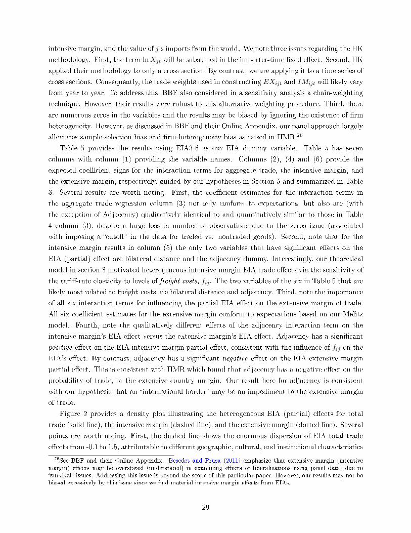
intensive margin, and the value of j's imports from the world. We note three issues regarding the HK
methodology. First, the term lnXjt will be subsumed in the importer-time xed eect. Second, HK
applied their methodology to only a cross section. By contrast, we are applying it to a time series of
cross sections. Consequently, the trade weights used in constructing EXijt and IMijt will likely vary
from year to year. To address this, BBF also considered in a sensitivity analysis a chain-weighting
technique. However, their results were robust to this alternative weighting procedure. Third, there
are numerous zeros in the variables and the results may be biased by ignoring the existence of rm
heterogeneity. However, as discussed in BBF and their Online Appendix, our panel approach largely
alleviates sample-selection bias and rm-heterogeneity bias as raised in HMR.26
Table 5 provides the results using EIA3-6 as our EIA dummy variable. Table 5 has seven
columns with column (1) providing the variable names. Columns (2), (4) and (6) provide the
expected coecient signs for the interaction terms for aggregate trade, the intensive margin, and
the extensive margin, respectively, guided by our hypotheses in Section 5 and summarized in Table
3. Several results are worth noting. First, the coecient estimates for the interaction terms in
the aggregate trade regression column (3) not only conform to expectations, but also are (with
the exception of Adjacency) qualitatively identical to and quantitatively similar to those in Table
4 column (3), despite a large loss in number of observations due to the zeros issue (associated
with imposing a cuto in the data for traded vs. nontraded goods). Second, note that for the
intensive margin results in column (5) the only two variables that have signicant eects on the
EIA (partial) eect are bilateral distance and the adjacency dummy. Interestingly, our theoretical
model in section 3 motivated heterogeneous intensive margin EIA trade eects via the sensitivity of
the tari-rate elasticity to levels of freight costs, fij . The two variables of the six in Table 5 that are
likely most related to freight costs are bilateral distance and adjacency. Third, note the importance
of all six interaction terms for inuencing the partial EIA eect on the extensive margin of trade.
All six coecient estimates for the extensive margin conform to expectations based on our Melitz
model. Fourth, note the qualitatively dierent eects of the adjacency interaction term on the
intensive margin's EIA eect versus the extensive margin's EIA eect. Adjacency has a signicant
positive eect on the EIA intensive margin partial eect, consistent with the inuence of fij on the
EIA's eect. By contrast, adjacency has a signicant negative eect on the EIA extensive margin
partial eect. This is consistent with HMR which found that adjacency has a negative eect on the
probability of trade, or the extensive country margin. Our result here for adjacency is consistent
with our hypothesis that an international border may be an impediment to the extensive margin
of trade.
Figure 2 provides a density plot illustrating the heterogeneous EIA (partial) eects for total
trade (solid line), the intensive margin (dashed line), and the extensive margin (dotted line). Several
points are worth noting. First, the dashed line shows the enormous dispersion of EIA total trade
eects from -0.1 to 1.5, attributable to dierent geographic, cultural, and institutional characteristics
26See BBF and their Online Appendix. Besedes and Prusa (2011) emphasize that extensive margin (intensivemargin) eects may be overstated (understated) in examining eects of liberalizations using panel data, due tosurvival issues. Addressing this issue is beyond the scope of this particular paper. However, our results may not bebiased excessively by this issue since we nd material intensive margin eects from EIAs.
29
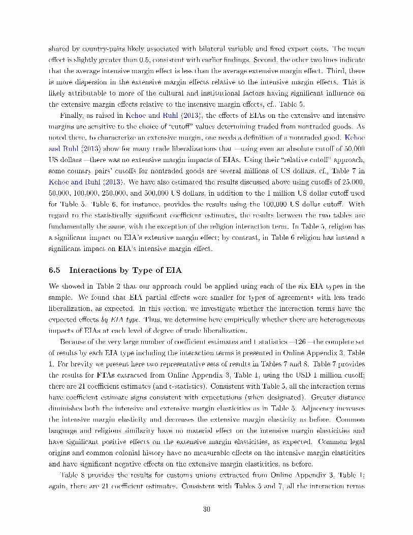
shared by country-pairs likely associated with bilateral variable and xed export costs. The mean
eect is slightly greater than 0.5, consistent with earlier ndings. Second, the other two lines indicate
that the average intensive margin eect is less than the average extensive margin eect. Third, there
is more dispersion in the extensive margin eects relative to the intensive margin eects. This is
likely attributable to more of the cultural and institutional factors having signicant inuence on
the extensive margin eects relative to the intensive margin eects, cf., Table 5.
Finally, as raised in Kehoe and Ruhl (2013), the eects of EIAs on the extensive and intensive
margins are sensitive to the choice of cuto values determining traded from nontraded goods. As
noted there, to characterize an extensive margin, one needs a denition of a nontraded good. Kehoe
and Ruhl (2013) show for many trade liberalizations that using even an absolute cuto of 50,000
US dollars there was no extensive margin impacts of EIAs. Using their relative cuto approach,
some country pairs' cutos for nontraded goods are several millions of US dollars, cf., Table 7 in
Kehoe and Ruhl (2013). We have also estimated the results discussed above using cutos of 25,000,
50,000, 100,000, 250,000, and 500,000 US dollars, in addition to the 1 million US dollar cuto used
for Table 5. Table 6, for instance, provides the results using the 100,000 US dollar cuto. With
regard to the statistically signicant coecient estimates, the results between the two tables are
fundamentally the same, with the exception of the religion interaction term. In Table 5, religion has
a signicant impact on EIA's extensive margin eect; by contrast, in Table 6 religion has instead a
signicant impact on EIA's intensive margin eect.
6.5 Interactions by Type of EIA
We showed in Table 2 that our approach could be applied using each of the six EIA types in the
sample. We found that EIA partial eects were smaller for types of agreements with less trade
liberalization, as expected. In this section, we investigate whether the interaction terms have the
expected eects by EIA type. Thus, we determine here empirically whether there are heterogeneous
impacts of EIAs at each level of degree of trade liberalization.
Because of the very large number of coecient estimates and t-statistics 126 the complete set
of results by each EIA type including the interaction terms is presented in Online Appendix 3, Table
1. For brevity we present here two representative sets of results in Tables 7 and 8. Table 7 provides
the results for FTAs extracted from Online Appendix 3, Table 1, using the USD 1 million cuto;
there are 21 coecient estimates (and t-statistics). Consistent with Table 5, all the interaction terms
have coecient estimate signs consistent with expectations (when designated). Greater distance
diminishes both the intensive and extensive margin elasticities as in Table 5. Adjacency increases
the intensive margin elasticity and decreases the extensive margin elasticity as before. Common
language and religious similarity have no material eect on the intensive margin elasticities and
have signicant positive eects on the extensive margin elasticities, as expected. Common legal
origins and common colonial history have no measurable eects on the intensive margin elasticities
and have signicant negative eects on the extensive margin elasticities, as before.
Table 8 provides the results for customs unions extracted from Online Appendix 3, Table 1;
again, there are 21 coecient estimates. Consistent with Tables 5 and 7, all the interaction terms
30
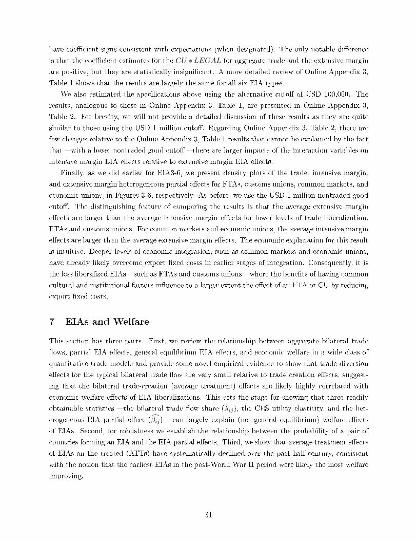
have coecient signs consistent with expectations (when designated). The only notable dierence
is that the coecient estimates for the CU ∗LEGAL for aggregate trade and the extensive margin
are positive, but they are statistically insignicant. A more detailed review of Online Appendix 3,
Table 1 shows that the results are largely the same for all six EIA types.
We also estimated the specications above using the alternative cuto of USD 100,000. The
results, analogous to those in Online Appendix 3, Table 1, are presented in Online Appendix 3,
Table 2. For brevity, we will not provide a detailed discussion of these results as they are quite
similar to those using the USD 1 million cuto. Regarding Online Appendix 3, Table 2, there are
few changes relative to the Online Appendix 3, Table 1 results that cannot be explained by the fact
that with a lower nontraded good cuto there are larger impacts of the interaction variables on
intensive margin EIA eects relative to extensive margin EIA eects.
Finally, as we did earlier for EIA3-6, we present density plots of the trade, intensive margin,
and extensive margin heterogeneous partial eects for FTAs, customs unions, common markets, and
economic unions, in Figures 3-6, respectively. As before, we use the USD 1 million nontraded good
cuto. The distinguishing feature of comparing the results is that the average extensive margin
eects are larger than the average intensive margin eects for lower levels of trade liberalization,
FTAs and customs unions. For common markets and economic unions, the average intensive margin
eects are larger than the average extensive margin eects. The economic explanation for this result
is intuitive. Deeper levels of economic integration, such as common markets and economic unions,
have already likely overcome export xed costs in earlier stages of integration. Consequently, it is
the less liberalized EIAs such as FTAs and customs unions where the benets of having common
cultural and institutional factors inuence to a larger extent the eect of an FTA or CU by reducing
export xed costs.
7 EIAs and Welfare
This section has three parts. First, we review the relationship between aggregate bilateral trade
ows, partial EIA eects, general equilibrium EIA eects, and economic welfare in a wide class of
quantitative trade models and provide some novel empirical evidence to show that trade diversion
eects for the typical bilateral trade ow are very small relative to trade creation eects, suggest-
ing that the bilateral trade-creation (average treatment) eects are likely highly correlated with
economic welfare eects of EIA liberalizations. This sets the stage for showing that three readily
obtainable statistics the bilateral trade ow share (λij), the CES utility elasticity, and the het-
erogeneous EIA partial eect (βij) can largely explain (net general equilibrium) welfare eects
of EIAs. Second, for robustness we establish the relationship between the probability of a pair of
countries forming an EIA and the EIA partial eects. Third, we show that average treatment eects
of EIAs on the treated (ATTs) have systematically declined over the past half century, consistent
with the notion that the earliest EIAs in the post-World War II period were likely the most welfare
improving.
31
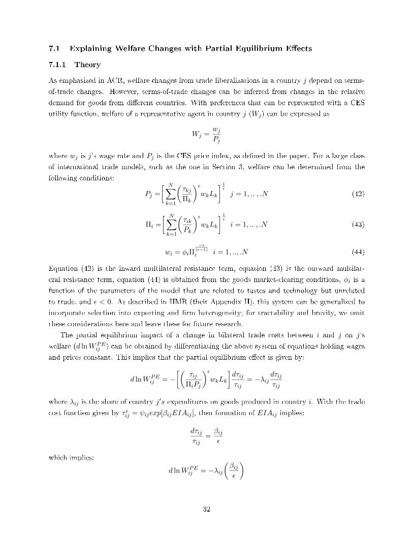
7.1 Explaining Welfare Changes with Partial Equilibrium Eects
7.1.1 Theory
As emphasized in ACR, welfare changes from trade liberalizations in a country j depend on terms-
of-trade changes. However, terms-of-trade changes can be inferred from changes in the relative
demand for goods from dierent countries. With preferences that can be represented with a CES
utility function, welfare of a representative agent in country j (Wj) can be expressed as
Wj =wjPj
where wj is j's wage rate and Pj is the CES price index, as dened in the paper. For a large class
of international trade models, such as the one in Section 3, welfare can be determined from the
following conditions:
Pj =
[ N∑k=1
(τkjΠk
)εwkLk
] 1ε
j = 1, .. , .N (42)
Πi =
[ N∑k=1
(τikPk
)εwkLk
] 1ε
i = 1, .. , .N (43)
wi = φiΠ−ε
(ε−1)
i i = 1, .., .N (44)
Equation (42) is the inward multilateral resistance term, equation (43) is the outward multilat-
eral resistance term, equation (44) is obtained from the goods market-clearing conditions, φi is a
function of the parameters of the model that are related to tastes and technology but unrelated
to trade, and ε < 0. As described in HMR (their Appendix II), this system can be generalized to
incorporate selection into exporting and rm heterogeneity; for tractability and brevity, we omit
these considerations here and leave these for future research.
The partial equilibrium impact of a change in bilateral trade costs between i and j on j's
welfare (d lnWPEij ) can be obtained by dierentiating the above system of equations holding wages
and prices constant. This implies that the partial equilibrium eect is given by:
d lnWPEij = −
[(τij
ΠiPj
)εwkLk
]dτijτij
= −λijdτijτij
where λij is the share of country j′s expenditures on goods produced in country i. With the trade
cost function given by τ εij = ψijexp[βijEIAij ], then formation of EIAij implies:
dτijτij
=βijε
which implies:
d lnWPEij = −λij
(βijε
)
32
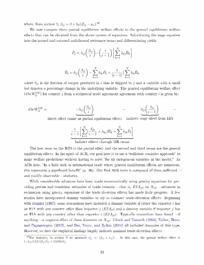
where, from section 2, βij = β + bZ(Zij − µz).27
We now compare these partial equilibrium welfare eects to the general equilibrium welfare
eects that can be obtained from the above system of equations. Substituting the wage equation
into the inward and outward multilateral resistance terms and dierentiating yields:
Pj = λij
(βijε
)−(
ε
ε− 1
)[ N∑k=1
λkjΠk
]
Πi = δij
(βijε
)−
N∑k=1
δikPk +1
(ε− 1))
N∑k=1
δikΠk
where δij is the fraction of output produced in i that is shipped to j and a variable with a small
hat denotes a percentage change in the underlying variable. The general equilibrium welfare eect
(d lnWGEij ) for country j from a reciprocal trade agreement agreement with country i is given by:
d lnWGEij = −λij
(βijε
)︸ ︷︷ ︸
direct eect (same as partial equilbirum eect)
− δji
(βjiε− 1
)︸ ︷︷ ︸
indirect wage eect from EIA
−
ε
ε− 1
[ N∑k=1
(δjkε− 1
+ λkj)Πk +N∑k=1
δjkPk
]︸ ︷︷ ︸
Indirect eects through MR terms
The rst term on the RHS is the partial eect and the second and third terms are the general
equilibrium eects. In the spirit of ACR, our goal here is to use a sucient statistics approach to
make welfare predictions without having to solve for all endogenous variables in the model. As
ACR note, In a eld such as international trade where general equilibrium eects are numerous,
this represents a signicant benet (p. 96). Our rst RHS term is composed of three sucient
and readily observable statistics.
While considerable advances have been made econometically using gravity equations for pro-
viding precise and consistent estimates of trade creation that is, EIAijt on Xijt advances in
estimation using gravity equations of the trade diversion eects has made little progress. A few
studies have incorporated dummy variables to try to estimate trade-diversion eects. Beginning
with Frankel (1997), some researchers have included a dummy variable if either the exporter i has
an EIA with any country other than importer j (EIAit) and a dummy variable if importer j has
an EIA with any country other than exporter i (EIAjt). Typically researchers have found if
anything a negative eect of these dummies on Xijt. Ghosh and Yamarik (2004), Eicher, Henn,
and Papageorgiou (2012), and Dai, Yotov, and Zylkin (2014) all included dummies of this type.
However, to date the empirical ndings largely indicate minimal trade diversion eects.
27For instance, in section 3 we assumed τ εij = (fij + tij)ε. In this case, the partial welfare eect is
(−λij/ε)(1/(fij/tij + 1))d ln tεij .
33
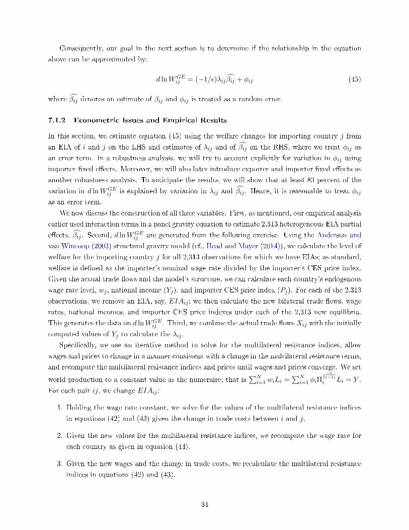
Consequently, our goal in the next section is to determine if the relationship in the equation
above can be approximated by:
d lnWGEij = (−1/ε)λij βij + φij (45)
where βij denotes an estimate of βij and φij is treated as a random error.
7.1.2 Econometric Issues and Empirical Results
In this section, we estimate equation (45) using the welfare changes for importing country j from
an EIA of i and j on the LHS and estimates of λij and of βij on the RHS, where we treat φij as
an error term. In a robustness analysis, we will try to account explicitly for variation in φij using
importer xed eects. Moreover, we will also later introduce exporter and importer xed eects as
another robustness analysis. To anticipate the results, we will show that at least 83 percent of the
variation in d lnWGEij is explained by variation in λij and βij . Hence, it is reasonable to treat φij
as an error term.
We now discuss the construction of all three variables. First, as mentioned, our empirical analysis
earlier used interaction terms in a panel gravity equation to estimate 2,313 heterogeneous EIA partial
eects, βij . Second, d lnWGEij are generated from the following exercise. Using the Anderson and
van Wincoop (2003) structural gravity model (cf., Head and Mayer (2014)), we calculate the level of
welfare for the importing country j for all 2,313 observations for which we have EIAs; as standard,
welfare is dened as the importer's nominal wage rate divided by the importer's CES price index.
Given the actual trade ows and the model's structure, we can calculate each country's endogenous
wage rate level, wj , national income (Yj), and importer CES price index (Pj). For each of the 2,313
observations, we remove an EIA, say, EIAij ; we then calculate the new bilateral trade ows, wage
rates, national incomes, and importer CES price indexes under each of the 2,313 new equilibria.
This generates the data on d lnWGEij . Third, we combine the actual trade ows Xij with the initially
computed values of Yj to calculate the λij .
Specically, we use an iterative method to solve for the multilateral resistance indices, allow
wages and prices to change in a manner consistent with a change in the multilateral resistance terms,
and recompute the multilateral resistance indices and prices until wages and prices converge. We set
world production to a constant value as the numeraire; that is∑N
i=1wiLi =∑N
i=1 φiΠ−ε
(ε−1)
i Li = Y .
For each pair ij, we change EIAij :
1. Holding the wage rate constant, we solve for the values of the multilateral resistance indices
in equations (42) and (43) given the change in trade costs between i and j.
2. Given the new values for the multilateral resistance indices, we recompute the wage rate for
each country as given in equation (44).
3. Given the new wages and the change in trade costs, we recalculate the multilateral resistance
indices in equations (42) and (43).
34
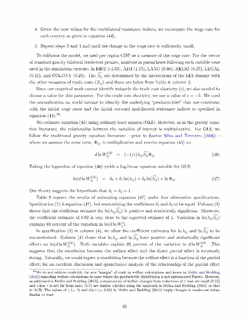
4. Given the new values for the multilateral resistance indices, we recompute the wage rate for
each country as given in equation (44).
5. Repeat steps 3 and 4 and until the change in the wage rate is suciently small.
To calibrate the model, we used per capita GDP as a measure of the wage rate. For the vector
of standard gravity bilateral trade-cost proxies, numbers in parentheses following each variable were
used in the simulation exercise: ln DIST (-1.03), ADJ (1.15), LANG (0.60), RELIG (0.25), LEGAL
(0.41), and COLONY (0.25). The βij are determined by the interactions of the EIA dummy with
the other measures of trade costs (Zij) and these are taken from Table 4, column 3.
Since our empirical work cannot identify uniquely the trade cost elasticity (ε), we also needed to
choose a value for this parameter. For the trade cost elasticity, we use a value of ε = −5. We used
the normalization on world income to identify the underlying productivities that are consistent
with the initial wage rates and the initial outward multilateral resistance indices as specied in
equation (44).28
We estimate equation (45) using ordinary least squares (OLS). However, as in the gravity equa-
tion literature, the relationship between the variables of interest is multiplicative. For OLS, we
follow the traditional gravity equation literature prior to Santos Silva and Tenreyro (2006)
where we assume the error term, Φij , is multiplicative and rewrite equation (45) as:
d lnWGEij = (−1/ε)λij βijΦij (46)
Taking the logarithm of equation (46) yields a log-linear equation suitable for OLS:
ln(d lnWGEij ) = δ0 + δ1 ln(λij) + δ2 ln(βij) + ln Φij . (47)
Our theory suggests the hypothesis that δ1 = δ2 = 1.
Table 9 reports the results of estimating equation (47) under four alternative specications.
Specication (1) is equation (47), but constraining the coecients δ1 and δ2 to be equal. Column (3)
shows that the coecient estimate for ln(λij βij) is positive and statistically signicant. Moreover,
the coecient estimate of 0.92 is very close to the expected estimate of 1. Variation in ln(λij βij)
explains 83 percent of the variation in ln(d lnW ij ).
In specication (2) in column (4), we allow the coecient estimates for lnλij and ln βij to be
unconstrained. Column (4) shows that lnλij and ln βij have positive and statistically signicant
eects on ln(d lnWGEij ). Both variables explain 85 percent of the variation in d lnWGE
ij . This
suggests that the correlation between the welfare eect and the direct partial eect is extremely
strong. Naturally, we would expect a correlation because the welfare eect is a function of the partial
eect; for an excellent discussion and quantitative analysis of the relationship of the partial eect
28We do not address explicitly the new margin of trade in welfare calculations and issues in Melitz and Redding(2015) regarding welfare calculations in cases where the productivity distribution is not untruncated Pareto. However,as addressed in Melitz and Redding (2015), computations of welfare changes from reductions of τ that are small (0.25)and when τ is not far from unity (1.5) are similar whether using the approach in Melitz and Redding (2015) or thatin ACR. The values of γ (= 4) and d ln τ (= 0.25) in Melitz and Redding (2015) imply changes in trade-cost valuessimilar to ours.
35
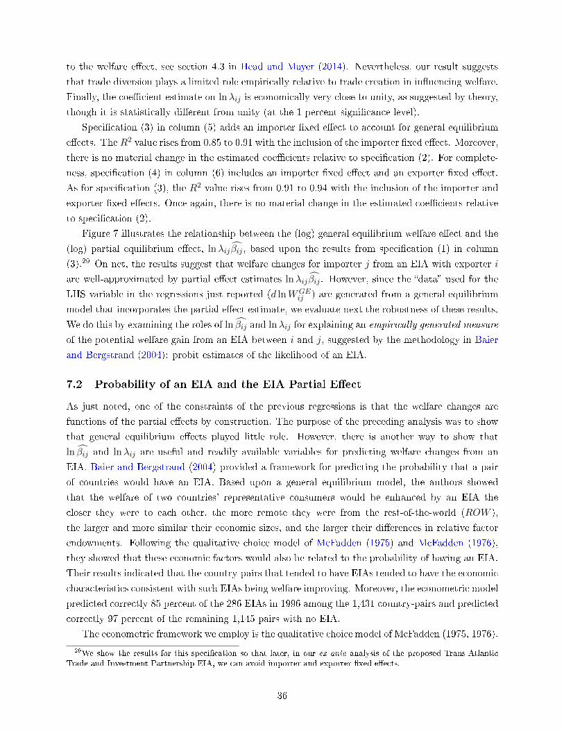
to the welfare eect, see section 4.3 in Head and Mayer (2014). Nevertheless, our result suggests
that trade diversion plays a limited role empirically relative to trade creation in inuencing welfare.
Finally, the coecient estimate on lnλij is economically very close to unity, as suggested by theory,
though it is statistically dierent from unity (at the 1 percent signicance level).
Specication (3) in column (5) adds an importer xed eect to account for general equilibrium
eects. The R2 value rises from 0.85 to 0.91 with the inclusion of the importer xed eect. Moreover,
there is no material change in the estimated coecients relative to specication (2). For complete-
ness, specication (4) in column (6) includes an importer xed eect and an exporter xed eect.
As for specication (3), the R2 value rises from 0.91 to 0.94 with the inclusion of the importer and
exporter xed eects. Once again, there is no material change in the estimated coecients relative
to specication (2).
Figure 7 illustrates the relationship between the (log) general equilibrium welfare eect and the
(log) partial equilibrium eect, lnλij βij , based upon the results from specication (1) in column
(3).29 On net, the results suggest that welfare changes for importer j from an EIA with exporter i
are well-approximated by partial eect estimates lnλij βij . However, since the data used for the
LHS variable in the regressions just reported (d lnWGEij ) are generated from a general equilibrium
model that incorporates the partial eect estimate, we evaluate next the robustness of these results.
We do this by examining the roles of ln βij and lnλij for explaining an empirically generated measure
of the potential welfare gain from an EIA between i and j, suggested by the methodology in Baier
and Bergstrand (2004): probit estimates of the likelihood of an EIA.
7.2 Probability of an EIA and the EIA Partial Eect
As just noted, one of the constraints of the previous regressions is that the welfare changes are
functions of the partial eects by construction. The purpose of the preceding analysis was to show
that general equilibrium eects played little role. However, there is another way to show that
ln βij and lnλij are useful and readily available variables for predicting welfare changes from an
EIA. Baier and Bergstrand (2004) provided a framework for predicting the probability that a pair
of countries would have an EIA. Based upon a general equilibrium model, the authors showed
that the welfare of two countries' representative consumers would be enhanced by an EIA the
closer they were to each other, the more remote they were from the rest-of-the-world (ROW ),
the larger and more similar their economic sizes, and the larger their dierences in relative factor
endowments. Following the qualitative choice model of McFadden (1975) and McFadden (1976),
they showed that these economic factors would also be related to the probability of having an EIA.
Their results indicated that the country-pairs that tended to have EIAs tended to have the economic
characteristics consistent with such EIAs being welfare improving. Moreover, the econometric model
predicted correctly 85 percent of the 286 EIAs in 1996 among the 1,431 country-pairs and predicted
correctly 97 percent of the remaining 1,145 pairs with no EIA.
The econometric framework we employ is the qualitative choice model of McFadden (1975, 1976).
29We show the results for this specication so that later, in our ex ante analysis of the proposed Trans-AtlanticTrade and Investment Partnership EIA, we can avoid importer and exporter xed eects.
36
A qualitative choice model can be derived from an underlying latent variable model. For instance,
let y∗ denote an unobserved (or latent) variable, where for simplicity we ignore the observation
subscript. As in Wooldridge (2000), let y∗ represent the dierence in utility levels from an action
(the formation of an FTA), where:
y∗ = ς0 + xς + ε (48)
where x is a vector of explanatory variables (i.e., common economic characteristics), ς is a vector
of parameters, and error term ε is assumed to be independent of x and to have a standard normal
distribution. In the context of this model, y∗ = min(∆Ui,∆Uj). Hence, both countries' consumers
need to benet from an EIA for their governments to form one. Since y∗ is unobservable, we denean indicator variable, EIA which takes the value 1 if two countries have an EIA (indicating y∗ > 0),
and 0 otherwise (indicating y∗ ≤ 0). The response probability, P , for EIA is:
P (EIA = 1) = P (y∗ > 0) = G(ς0 + xς) (49)
where G(·) is the standard normal cumulative distribution function, which ensures that P (EIA = 1)
lies between 0 and 1.
In this context, we predicted the probabilities of country-pairs having EIAs for the nine years
1970, 1975, ..., 2010 using similar economic characteristics; the probit results are provided in Online
Appendix 4. The relationships between the economic characteristics with the probabilities are qual-
itatively very similar across the nine years and are consistent with ndings in Baier and Bergstrand
(2004). As expected based upon the theoretical framework in Baier and Bergstrand (2004), the like-
lihood of an EIA is negatively related to distance, positively related to economic size (joint GDP),
and negatively related to GDP dissimilarity. We also nd that that the probability of an EIA is
positively related to having a common primary language and religious similarity. In the context of
the Baier-Bergstrand model, the country-pairs that tend to have EIAs tend to have the economic
characteristics consistent with such EIAs being welfare improving.
Our goal in this section is to determine whether ln βij and lnλij can also explain the variation
in the probabilities of EIAs, which serve as proxies for the welfare gains of a country-pair from an
EIA. Table 10 presents the results of ve alternative specications. The number of observations
is limited to 2,360, as these are the number of estimates of ln βij from our earlier results. The
rst specication, shown in column (3), regresses lnP (EIAijt) on lnλij , ln βij , and a constant.
Two results are worth noting. First, both variables have the expected qualitative relationship with
lnP (EIAijt); as lnP (EIAijt) serves as a proxy for d lnWGEij , we cannot assign a specic expected
quantitative value for the coecients. Second, we note that the pseudo R2 value is 53 percent.
One possible concern, however, is that the ln βij work well to explain the probability of an
EIA because the ln βij themselves will tend to be higher when variable and xed export costs
are low, as our theory suggested. Consequently, ln βij may have an economically and statistically
signicant eect simply because ln βij and lnP (EIAijt) are inuenced by common variables, such
as bilateral distance, adjacency, etc. To address the robustness of our results, we considered several
other specications. Column (4) adds the log of bilateral distance to the regression. Column (4)
37
shows that while lnDISTij helps to explain lnP (EIAijt) lnλij and ln βij still have signicant
explanatory power. Moreover, adding only distance increases the explanatory power from 53 percent
to 85 percent. In the next sensitivity analysis, we included bilateral distance as well as all the other
variables used earlier to explain variable and xed export costs (and which are determinants of
the predicted probabilities, as shown in Online Appendix 4). Column (5) shows that although all
these observables are statistically signicant in explaining lnP (EIAijt) lnλij and ln βij still retain
signicant explanatory power. Moreover, the coecient estimates for lnλij and ln βij hardly change
at all. The specication in column (6) adds an importer xed eect. As shown in column (6), this
has no material eect on the explanatory power of lnλij and ln βij . Finally, for completeness, the
specication in column (7) adds both an importer and exporter xed eect. Although the coecient
estimate for lnλij becomes negative and marginally signicant, the coecient estimate for ln βij
has no material change.
7.3 Timing of Average Treatment Eects on the Treated
We consider one other approach to show that the partial eects of EIAs are consistent with welfare
improvement from EIAs. As discussed in BB and BBF, one of the benets of using panel data to
estimate partial eects is that it can account for the endogeneity of EIAs. However, one of the
drawbacks of estimating partial eects using panel data is that the treatment eect is assumed to
be constant across all years; in our analysis, that is 1965-2010. As now apparent, a main thrust of
our paper has been to show that partial eects vary by country-pair; however, we have not allowed
any variation in treatment eects over time. In this section, we examine in particular the average
treatment eects on treated pairs (ATTs) across nine periods.
We now provide motivation for estimating the ATT for each of nine periods. Following the
logic of Baier and Bergstrand (2004), if country-pairs' governments are maximizing welfare of
their consumers, then the EIAs that are formed will likely have economic characteristics consistent
with welfare maximization. For instance, Baier and Bergstrand (2004) showed theoretically that
if country-pairs are physically close and have large and similar GDPs, they will benet more from
an EIA. Baier and Bergstrand (2009) showed for nine cross-sections 5-years apart (1960-2000) that
countries that are close and have large and similar GDPs tend to have EIAs. Moreover, Bergstrand,
Egger, and Larch (2015) show that the countries that are closer and have larger and more similar
GDPs have higher probabilities of forming EIAs sooner. If indeed country-pairs' governments are
maximizing their consumers' welfare, then not only is the probability higher that they will form an
EIA earlier but in the context of our paper the ATTs of the EIAs should be larger in earlier
years than later years.
In this section, we examine the ATTs from our panel data estimates. That is, using the method-
ology described earlier, we have estimates βij for every country-pair that was treated. We then
group the partial eects by nine periods in which these EIAs formed: 1965-1970, 1965-1975, 1965-
1980, ..., 1965-2010. We then take the average of the partial eects for each of these nine periods.
These are what we term here the ATTs for each period.30 These are reported in Table 11.
30Note that the approach here uses a parametric approach to derive ATTs. This diers from the nonparametric
38
Table 11 has six columns. The rst column provides the period in which all EIAs were formed
in that period.31 The second column provides the (cumulative) number of EIAs formed. The third
column provides the ATTs for EIAs formed during that period. The fourth column provides the
standard deviation of the ATTs during that period. The fth column provides the percentage of
the EIA number of estimated partial eects that were positive during that period. Finally, column
(6) reports estimates of the average treatment eect on the untreated, and we will explain shortly
the insight from calculating those.
There are several important ndings. First, column (3) shows that the ATTs in the earlier years
are the highest. The ATT by period falls (though not strictly monotonically) over time indicating
that the EIAs that formed rst had the highest ATTs, implying given our discussion above and
Figure 7 the highest welfare gains. This result is consistent with Bergstrand, Egger, and Larch
(2015).
Second, column (5) indicates that the number of negative partial eects is very low. For the
period 1965-1995, 99 percent of the ATTs were positive. This result is consistent with the ndings
shown in Figures 2-6 earlier.
Third, we also report in column (6) a measure called the average treatment eect on the un-
treated (ATU). The ATU is not as prevalent in econometric reporting as the ATT; the ATT makes
intuitive sense because typically one is interested in measuring the eect of a treatment on those
actually treated. However, for our purposes the ATU is informative for two reasons. One, the ATU
in any given period should be smaller than the ATT. That the ATT in a period exceeds the ATU
suggests again recalling the earlier discussion and Figure 7 that the welfare gains were highest for
the countries that formed EIAs in the designated period. Two, just as the ATTs decline over time,
the ATUs decline over time as well. This suggests that over time as some country-pairs without
EIAs form ones, the remaining country-pairs have less to gain in trade and welfare; this should be
the case.
8 Ex Ante Predictions for the Proposed Transatlantic Trade and
Investment Partnership
Our analysis in this paper suggests three readily observable statistics to approximate general
equilibrium welfare gains of EIAs and in particular highlights the benets of using dummy
variables and treatment eects to help quantify the trade and welfare eects of EIAs. Where might
such methodologies be warranted?
In April 2007, one of the rst in-depth discussions of a potential Transatlantic Trade and In-
vestment Partnership (TTIP) agreement took place at a European Union-United States (EU-US)
approach used in Baier and Bergstrand (2009). In that paper, the authors used nonparametric (matching) techniquesto estimate ATTs. Such techniques were useful to identify in a time-series of cross-sections the average treatmenteects on treated pairs over time also, accounting (in cross-sections) for the endogeneity of EIAs using treated andcontrol groups. See that paper for such an alternative technique, beyond the scope of this already lengthy paper.
31The Baier-Bergstrand data set is a comprehensive data set of EIA formations from 1950 to 2010 for 195 countriesin the world.
39
summit. This summit inspired the European Commission to award a consortium of economic con-
sulting rms to study quantitatively the potential impacts on trade, investment, and welfare of
reductions in non-tari measures (NTMs) on trade and investment; NTMs remain the main policy
barriers to trade and investment between two of the largest economic regions in the world. Fur-
thermore, the study authorized the quantitative analysis of reductions in the remaining taris on
goods and services, which most observers know are quite low already. A major contribution of this
analysis, reported in Berden, Francois, Tamminen, Thelle, and Wymenga (2010), was developing a
methodology to estimate ad valorem equivalents of the non-tari barriers to international trade and
investment, which was no small task.32 A subsequent study, Francois, Manchin, Norberg, Pindyuk,
and Tornberger (2013), extended the analysis in Berden et al. (2010) to provide trade and welfare
eect estimates of the proposed TTIP.
In this section, we use the methodology of this paper to conduct an ex ante analysis of the
TTIP, and then compare the results to those in Francois et al. (2013). Because of the substantive
length of this paper already, we constrain our analysis here to aggregate (nal goods) trade eects
and welfare gains only; we leave analysis of foreign direct investment and sectoral decomposition for
others. Basically, we calculated βij for the US (both as importer and exporter) with 26 members of
the EU (for which data was readily available) using our regression coecient estimates from earlier
in the paper. We combined these with estimates of λij , the shares of i's goods in j's domestic
expenditures (expressed in percentages).
Table 12 provides the values of the βij and λij for all of the 52 country-pairs; their products are
in column (5). Several results are worth noting. First, virtually all of the βij are positive. Excluding
the two negative βij estimates, the heterogeneous partial trade eects range from 0.0572 (about 5.9
percent) to 0.3838 (about 46.8 percent). The typical eect is about 23 percent, with heterogeneity
very similar to that shown earlier.
Second, column (4) reports the values of λij , expressed in percentages. Note that these values
are small, since exports and imports are only 15 percent of US expenditures and no single EU
exporter dominates exports to the US. We do not report yet the welfare eect; the reason is that
the welfare eect is sensitive to the CES utility parameter, labeled here ε (ε < 0).33 We will provide
shortly ex ante welfare eect predictions using representative values of −ε.34
It is useful to ask: Are these estimates plausible? Naturally, it would be benecial to have
some other estimates with which to compare. There is only a small number of analyses of TTIP,
summarized in a European Parliament study by Bendini and Micco (2014). However, according
to Bendini and Micco (2014), The principal study cited by the European Commission to support
the initiation of TTIP talks is Francois et al. (2013), mentioned above. Francois et al. (2013)
considered fundamentally two alternative approaches in their analysis. The rst was a set of Lim-
32The Academic Advisory Team for this study's methodology was James Anderson, Jerey Bergstrand, PeterEgger and Joseph Francois. The published study is Berden et al. (2010). The economic methodology is in Anderson,Bergstrand, Egger, and Francois (2008) and summarized in Berden et al. (2010). See also http://ntm.ecorys.com .
33As discussed in ACR, ε can have alternative interpretations depending on the underlying model.34Although the welfare gains for the US are simply the sum of the bilateral welfare gains with each EU exporter,
the welfare gains of the EU as importer need to account for the relative importance of each country in the EU. Weused population shares to weight the relative importance of each bilateral welfare gain.
40
ited Scenarios; these addressed partial agreements that focused on tari reductions only, services
liberalization only, or procurement liberalization only. The second was a set of Full-edged Free
Trade Agreements. Within this set, they considered two alternative scenarios. One was a Less
Ambitious TTIP that included full (actually, 98 percent) tari removals and a 10 percent reduction
in (ad valorem estimates of) trade costs from nontari barriers (NTBs). The other was a More
Ambitious TTIP that included full tari removals and a 25 percent reduction in trade costs from
NTBs.35
However, at least one serious issue facing any comparison of welfare eects across studies is the
assumption on values of −ε. Unfortunately, Francois et al. (2013) does not report such values,
which will dier by sector in their work due to disaggregation. However, much of Francois et al.
(2013) is based upon estimates in Berden et al. (2010), for which estimated values of −ε rangedfrom 0.8 to 14.5. Consequently, comparison of welfare eects is dicult.
Because of this issue, it will be useful rst to compare predicted trade impacts. Our model's
predicted trade impacts are provided in column (3) of Table 12; these are heterogeneous across
partners. For the US as importer, for example, the (exponentiated) trade impacts range from -14
percent to 46 percent; only 2 of the 26 estimates are negative. The median estimate is 23 percent
(= exp (0.2037)). In Francois et al. (2013), the Less Ambitious TTIP scenario predicts a 16 percent
increase in US imports from the EU and the More Ambitious TTIP scenario predicts a 29 percent
increase in US imports from the EU. Thus, our estimates accord with those in Francois et al. (2013).
For the EU as importer, our (exponentiated) trade impacts are similar to the estimates for the US as
importer due to the symmetry in factors explaining the heterogeneous partial impacts. In Francois
et al. (2013), the Less Ambitious TTIP scenario predicts a 22 percent increase in EU imports from
the US and the More Ambitious TTIP scenario predicts a 35 percent increase in EU imports from
the US. Francois et al. (2013) estimates are higher primarily due to higher initial EU taris in their
model. In general, our partial trade impacts are similar to those in Francois et al. (2013), even
though that study does not report the bilateral partial trade impacts.
Finally, based upon our framework we can provide ex ante TTIP welfare impacts for both the
US and for the EU, which depend upon our choice of ε. A typical value of −ε is 3. In the context of
the Armington model, this corresponds with an elasticity of substitution of 4; in the Chaney (2008)
model, this corresponds with a productivity heterogeneity parameter of 4. Using our approach, the
TTIP ex ante welfare eect for the US as importer is 0.09 percent; given the strong symmetry in
our approach, the welfare eect for the EU is also 0.09 percent.36
Table 13 presents the welfare gains (in percent, national income) from Francois et al. (2013).
While not directly comparable to our estimates, they shed some light on the matter. First, EU
welfare gains are larger than US welfare gains; as Francois et al. (2013) note, they use higher initial
EU taris, based upon results from Berden et al. (2010). Second, the welfare gains increase for each
region as the degree of trade liberalization increases from a reduction in taris only all the way to
the More Ambitious TTIP scenario.
35Other issues were addressed also, but are not relevant for our comparison here to our results.36For ε = −7, the welfare eect is 0.04 percent for both countries; for ε = −1, the welfare eect for the US is 0.26
percent and for the EU is 0.27 percent.
41
While a direct comparison of welfare eects between our study and Francois et al. (2013) has
limitations, our results are suggestive. The results show that our approach provides some credible
ex ante estimates of the welfare gains from the TTIP. For a value of −ε = 3, our approach suggests
welfare gains from TTIP of about 0.09 percent for each of the US and the EU. Such gains are in line
with estimates based upon Francois et al. (2013), lying between the tari only and less ambitious
liberalization scenarios. Future studies using more precise estimates of ad valorem changes in taris
and non-tari barriers from TTIP beyond our limited and preliminary exercise here potentially
could provide even stronger support for the usefulness of our approach.
9 Conclusion
The following summarizes the contributions of this paper. Using a random coecients gravity
equation, we demonstrated extensive heterogeneity in EIAs' partial eects on trade ows beyond
dierences in degrees of trade liberalization, controlling for endogeneity using the panel techniques of
BB and BBF. Using an Armington theoretical trade model, we demonstrated why the heterogeneity
in partial eects of EIAs in gravity equations may be related to factors associated with variable trade
costs such as freight charges, inuencing the intensive product margin of trade. Using a Melitz-
type theoretical model, we demonstrated why the heterogeneity in partial eects of EIAs may be
related to factors associated with variable and xed export costs, inuencing the extensive product
margin of trade. Extending BBF, we demonstrated that six standard covariates explaining trade
ows (also used in HMR) have economically and statistically signicant impacts on the quantitative
partial eects of EIAs on trade ows. Distance and adjacency explain the heterogeneous EIA
eects on the intensive margins of trade. Distance, adjacency, language, religion, legal origins, and
colonial history explain the heterogeneous EIA eects on extensive margins of trade. Moreover, the
qualitatively dierent impacts of institutional variables versus cultural variables on the extensive
margin eect is consistent with the novel aspect of our Melitz model distinguishing policy from
non-policy exogenous export xed costs. We showed that 83 percent or more of the variation in
welfare eects for importers from EIAs could be explained by two readily observable statistics: the
share of the trade ow from i to j relative to importer j's expenditures (λij) and the heterogeneous
partial eect (βij). Moreover, in the spirit of Baier and Bergstrand (2004), we showed that 85
percent or more of the variation in the probability of an EIA between i and j could be explained by
the above two factors, along with bilateral distance. We showed that the average treatment eects
on the treated pairs were highest for the EIAs that formed the earliest, and then declined nearly
monotonically; this is consistent with Bergstrand, Egger, and Larch (2015) and the notion that the
earliest EIAs were formed by country-pairs with likely the most to gain in welfare from their EIAs.
In a comparison of our model's ex ante welfare gains predictions for the US and EU associated with
the proposed TTIP relative to those from the principal study cited by the European Parliament,
our ex ante welfare predictions lie between those suggested by Francois et al. (2013) for a Tari
Only and a Less Ambitious TTIP, providing support for the relevance of our approach.
Nevertheless, our approach in this paper could be enhanced in future work along at least two
42
dimensions. Theoretically, we have provided two models an Armington model and a Melitz model
to introduce heterogeneous EIA eects for intensive and extensive margins, respectively. Merging
the two models is not a trivial exercise mathematically due to the complexity of the model. And
although we provide guidance in Online Appendix 2 toward solving such a model, future work may
try to build such a model explicitly. Empirically, we have relied upon dummy variables and average
treatment eect estimates to capture the impacts on trade of tari rates and non-tari measures
from EIA formations, partly due to the paucity of good data on trade policies and partly due to the
benets of using a treatment eects approach. Continued advances in developing more credible
measures of tari and especially nontari barriers to capture ad valorem trade costs beyond the
techniques advanced in Anderson et al. (2008) and Berden et al. (2010) are needed, and such
rened continuous measures should be considered when estimating heterogenous eects of EIAs on
trade ows.
References
Anderson, J., J. Bergstrand, P. Egger, and J. Francois (2008): Non-Tari Barrier Study
Methodology, http://ntm.ecorys.com.
Anderson, J., and E. van Wincoop (2003): Gravity with Gravitas: A Solution to the Border
Puzzle, American Economic Review, 93(1), 170192.
Anderson, J., and E. van Wincoop (2004): Trade Costs, Journal of Economic Literature,
42(3), 691751.
Anderson, J., and Y. Yotov (2011): Terms of Trade and Global Eciency Eects of Free Trade
Agreements, NBER Working Paper No. 17003.
Arkolakis, C., A. Costinot, and A. Rodriguez-Clare (2012): New Trade Models, Same
Old Gains?, American Economic Review, 102(1), 94130.
Arkolakis, C., S. Demidova, P. Klenow, and A. Rodriguez-Clare (2008): Endogenous
Variety and the Gains from Trade, American Economic Review, 98(2), 444450.
Baier, S., and J. Bergstrand (2001): The Growth of World Trade: Taris, Transport Costs,
and Income Similarity, Journal of International Economics, 53(1), 127.
(2004): The Economic Determinants of Free Trade Agreements, Journal of International
Economics, 64(1), 2963.
(2007): Do Free Trade Agreements Actually Increase Members' International Trade?,
Journal of International Economics, 71(1), 7295.
(2009): Estimating the Eects of Free Trade Agreements on International Trade Flows
using Matching Econometrics, Journal of International Economics, 77(1), 6376.
43
Baier, S., J. Bergstrand, and M. Clance (2015): Preliminary Examination of Heterogeneous
Eects on International Trade of Economic Integration Agreements, in Trade Cooperation, ed.
by A. Dur, and M. Elsig, pp. 355373. Cambridge University Press, Cambridge, UK.
Baier, S., J. Bergstrand, and M. Feng (2014): Economic Integration Agreements and the
Margins of International Trade, Journal of International Economics, 93(2), 339350.
Baldwin, R., and J. Harrigan (2011): Zeros, Quality, and Space: Trade Theory and Trade
Evidence, American Economic Journal: Micoreconomics, 3(2), 6088.
Bendini, R., and P. D. Micco (2014): The Expected Impact of the TTIP on EU Member States
and Selected Third Countries, Directorate-General for External Policies, European Parliament.
Berden, K., J. Francois, S. Tamminen, M. Thelle, and P. Wymenga (2010): Non-Tari
Measures in EU-US Trade and Investment. ECORYS, The Netherlands.
Bergstrand, J., P. Egger, and M. Larch (2015): Economic Determinants of the Timing of
Preferential Trade Agreement Formations and Enlargements, Economic Inquiry, forthcoming.
Bergstrand, J., M. Larch, and Y. Yotov (2015): Economic Integration Agreements, Border
Eects, and Distance Elasticities in the Gravity Equation, European Economic Review, forth-
coming.
Besedes, T., and T. Prusa (2011): The Role of Extensive and Intensive Margins and Export
Growth, Journal of Development Economics, 96(2), 371379.
Cameron, A., and P. Trivedi (2005): Microeconometrics - Methods and Applications. Cambridge
University Press, Cambridge, United Kingdom.
Chaney, T. (2008): Distorted Gravity: The Intensive and Extensive Margins of International
Trade, American Economic Review, 98(4), 17071721.
Cheng, I., and H. Wall (2005): Controlling for Heterogeneity in Gravity Models of Trade and
Integration, Federal Reserve Bank of St. Louis Review, 87(1), 4963.
Cheong, J., D. Kwak, and K. Tang (2015): Heterogeneous Eects of Preferential Trade Agree-
ments, World Development, 66, 222236.
Cipollina, M., and L. Salvatici (2010): Reciprocal Trade Agreements in Gravity Models: A
Meta-Analysis, Review of Economic Literature, 18(1), 6380.
Dai, M., Y. Yotov, and T. Zylkin (2014): On the Trade-Diversion Eects of Free Trade
Agreements, Economics Letters, 122(2), 321325.
Eaton, J., and S. Kortum (2002): Technology, Geography and Trade, Econometrica, 70(5),
17411779.
44
Eaton, J., S. Kortum, and F. Kramarz (2011): An Anatomy of International Trade: Evidence
from French Firms, Econometrica, 79(5), 14531498.
Egger, P., M. Larch, K. Staub, and R. Winkelmann (2011): The Trade Eects of En-
dogenous Preferential Trade Agreements, American Economic Journal: Economic Policy, 3(3),
113143.
Eicher, T., C. Henn, and C. Papageorgiou (2012): Trade Creation and Diversion Revisited:
Accounting for Model Uncertainty and Natural Trading Partner Eects, Journal of Applied
Econometrics, 27(2), 296321.
Francois, J., M. Manchin, H. Norberg, O. Pindyuk, and P. Tornberger (2013): Reduc-
ing Transatlantic Barriers to Trade and Investment, CEPR.
Frankel, J. (1997): Regional Trading Blocs. Institute for International Economics, Washington,
DC.
Ghosh, S., and S. Yamarik (2004): Are Regional Trade Agreements Trade Creating?, Journal
of International Economics, 63(2), 369395.
Head, K., and T. Mayer (2014): Gravity Equations: Workhorse, Toolkit, and Cookbook, in
Handbook of Interantional Economics, Volume 4, ed. by G. Gopinath, E. Helpman, and K. Rogo.
Elsevier, Amsterdam.
Helpman, E., M. Melitz, and Y. Rubinstein (2008): Trading Partners and Trading Volumes,
Quarterly Journal of Economics, 123(2), 441487.
Horn, H., P. Mavroidis, and A. Sapir (2010): Beyond the WTO? An Anatomy of EU and US
Preferential Trade Agreements, The World Economy, 33(11), 15651588.
Hummels, D. (2007): transportation Costs and International Trade in teh Second Era of Global-
ization, Journal of Economic Perspectives, 21(3), 131154.
Hummels, D., and P. Klenow (2005): The Variety and Quality of a Nation's Exports, American
Economic Review, 95(3), 704723.
Hummels, D., and A. Skiba (2004): A Virtuous Circle? Regional Tari Liberalization and
Scale Economies in Transport, in: Estevadeordal, A., D. Rodrik, A. Taylor, and A. Velasco
(eds.): Integrating the Americas: FTAA and Beyond. Harvard University Press, Cambridge,
Massachusetts.
Kehoe, T., and K. Ruhl (2013): How Important is the New Goods Margin in International
Trade?, Journal of Political Economy, 121(2), 358392.
Kohl, T., S. Brakman, and H. Garretsen (2014): Do Trade Agreements Stimulate Interna-
tional Trade Dierently?, working paper.
45
Krautheim, S. (2012): Heterogeneous Firms, Exporter Networks and the Eect of Distance on
International Trade, Journal of International Economics, forthcoming.
McCallum, J. (1995): National Borders Matter, American Economic Review, 85(3), 615623.
McFadden, D. (1975): The Revealed Preferences of a Government Bureaucracy: Theory, Bell
Journal of Economics, 6, 401416.
(1976): Quantal Choice Analysis: A Survey, Annals of Economic and Social Measurement,
5, 363390.
Melitz, M., and S. Redding (2015): New Trade Models, New Welfare Implications, American
Economic Review, 105(3), 11051146.
Novy, D. (2013): International Trade without CES: Estimating Translog Gravity, Journal of
International Economics, 89(2), 271282.
Pavcnik, N. (2002): Trade Liberalization, Exit, and Productivity Improvements: Evidence from
Chilean Plants, Review of Economic Studies, 69, 245276.
Santos Silva, J., and S. Tenreyro (2006): The Log of Gravity, Review of Economics and
Statistics, 88(4), 641658.
Tinbergen, J. (1962): Shaping the World Economy: Suggestions for an International Economic
Policy. The Twentieth Century Fund, New York.
Trefler, D. (2004): The Long and Short of the Canada-U.S. Free Trade Agreement, American
Economic Review, 94(4), 870895.
Vicard, V. (2011): Determinants of Successful Regional Trade Agreements, Economics Letters,
111, 188190.
Wooldridge, J. (2000): Introductory Econometrics. South-Western, Chicago.
46
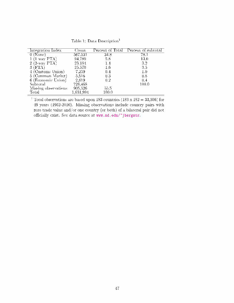
Table 1: Data Description1
Integration Index Count Percent of Total Percent of subtotal0 (None) 567,531 34.8 78.11 (1-way PTA) 94,789 5.8 13.02 (2-way PTA) 23,184 1.4 3.23 (FTA) 25,570 1.6 3.54 (Customs Union) 7,259 0.4 1.05 (Common Market) 5,516 0.3 0.86 (Economic Union) 2,619 0.2 0.4Subtotal 726,468 - 100.0Missing observations 905,526 55.5Total 1,631,994 100.0
1 Total observations are based upon 183 countries (183 x 182 = 33,306) for49 years (1962-2010). Missing observations include country pairs withzero trade value and/or one country (or both) of a bilateral pair did notocially exist. See data source at www.nd.edu/~jbergstr.
47
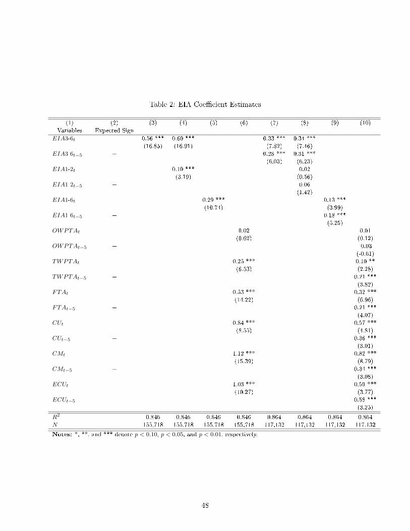
Table 2: EIA Coecient Estimates
(1) (2) (3) (4) (5) (6) (7) (8) (9) (10)
Variables Expected Sign
EIA3-6t + 0.56 *** 0.60 *** 0.33 *** 0.34 ***
(16.85) (16.91) (7.82) (7.46)
EIA3-6t−5 + 0.28 *** 0.31 ***
(6.03) (6.23)
EIA1-2t + 0.10 *** 0.02
(3.19) (0.56)
EIA1-2t−5 + 0.06
(1.42)
EIA1-6t + 0.29 *** 0.13 ***
(10.74) (3.99)
EIA1-6t−5 + 0.18 ***
(5.25)
OWPTAt + 0.02 0.01
(0.62) (0.12)
OWPTAt−5 + -0.03
(-0.61)
TWPTAt + 0.25 *** 0.10 **
(6.53) (2.28)
TWPTAt−5 + 0.21 ***
(3.82)
FTAt + 0.53 *** 0.32 ***
(14.22) (6.96)
FTAt−5 + 0.21 ***
(4.07)
CUt + 0.84 *** 0.57 ***
(8.55) (4.81)
CUt−5 + 0.36 ***
(3.01)
CMt + 1.12 *** 0.82 ***
(15.39) (8.79)
CMt−5 + 0.34 ***
(3.08)
ECUt 1.03 *** 0.59 ***
(10.27) (3.77)
ECUt−5 0.58 ***
(3.25)
R2 0.846 0.846 0.846 0.846 0.864 0.864 0.864 0.864
N 155,718 155,718 155,718 155,718 117,132 117,132 117,132 117,132
Notes: *, **, and *** denote p < 0.10, p < 0.05, and p < 0.01, respectively.
48
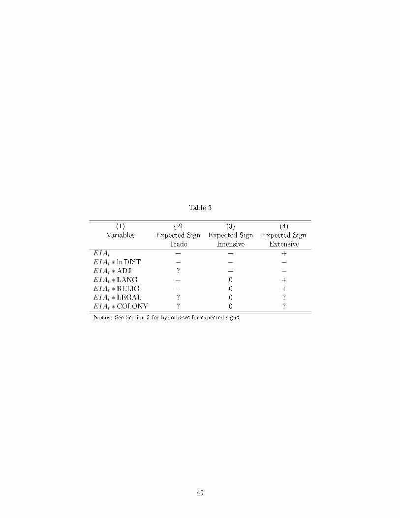
Table 3
(1) (2) (3) (4)Variables Expected Sign Expected Sign Expected Sign
Trade Intensive Extensive
EIAt + + +EIAt ∗ lnDIST − − −EIAt ∗ADJ ? + −EIAt ∗ LANG + 0 +EIAt ∗ RELIG + 0 +EIAt ∗ LEGAL ? 0 ?EIAt ∗ COLONY ? 0 ?
Notes: See Section 5 for hypotheses for expected signs.
49
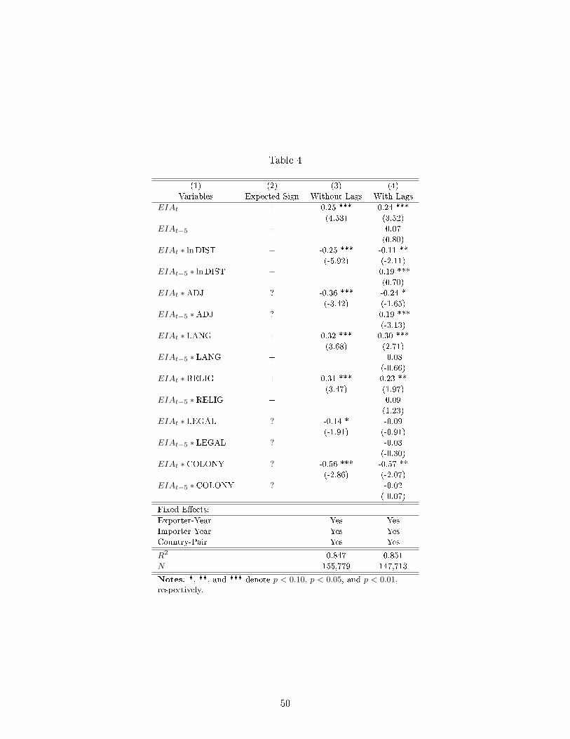
Table 4
(1) (2) (3) (4)
Variables Expected Sign Without Lags With Lags
EIAt + 0.25 *** 0.24 ***
(4.53) (3.52)
EIAt−5 + 0.07
(0.80)
EIAt ∗ lnDIST − -0.25 *** -0.11 **
(-5.92) (-2.11)
EIAt−5 ∗ lnDIST − -0.19 ***
(0.70)
EIAt ∗ADJ ? -0.36 *** -0.24 *
(-3.42) (-1.65)
EIAt−5 ∗ADJ ? -0.19 ***
(-3.13)
EIAt ∗ LANG + 0.32 *** 0.30 ***
(3.68) (2.71)
EIAt−5 ∗ LANG + -0.08
(-0.66)
EIAt ∗ RELIG + 0.31 *** 0.23 **
(3.47) (1.97)
EIAt−5 ∗ RELIG + 0.09
(1.23)
EIAt ∗ LEGAL ? -0.14 * -0.09
(-1.91) (-0.91)
EIAt−5 ∗ LEGAL ? -0.03
(-0.30)
EIAt ∗ COLONY ? -0.56 *** -0.57 **
(-2.86) (-2.07)
EIAt−5 ∗ COLONY ? -0.02
(-0.07)
Fixed Eects:
Exporter-Year Yes Yes
Importer-Year Yes Yes
Country-Pair Yes Yes
R2 0.847 0.851
N 155,779 147,713
Notes: *, **, and *** denote p < 0.10, p < 0.05, and p < 0.01,respectively.
50

Table 5
(1) (2) (3) (4) (5) (6) (7)
Expected Sign Expected Sign Expected Sign
Variables Trade Trade Intensive Intensive Extensive Extensive
EIAt + 0.23 *** + 0.07 ** + 0.16 ***
(6.94) (2.31) (4.08)
EIAt ∗ lnDIST − -0.24 *** − -0.09 *** − -0.15 ***
(-9.88) (-3.83) (-5.18)
EIAt ∗ADJ ? 0.03 + 0.24 *** − -0.21 ***
(0.58) (4.23) (-3.00)
EIAt ∗ LANG + 0.20 *** 0 0.02 + 0.17 ***
(3.82) (0.47) (2.92)
EIAt ∗ RELIG + 0.23 *** 0 0.07 + 0.16 ***
(4.51) (1.39) (2.75)
EIAt ∗ LEGAL ? -0.12 *** 0 0.02 ? -0.14 ***
(-2.80) (0.60) (-2.92)
EIAt ∗ COLONY ? -0.25 ** 0 0.10 ? -0.35 ***
(-2.52) (1.02) (-3.04)
Fixed Eects:
Exporter-Year Yes Yes Yes
Importer-Year Yes Yes Yes
Country-Pair Yes Yes Yes
R2 0.912 0.821 0.824
N 70,173 70,173 70,173
Notes: *, **, and *** denote p < 0.10, p < 0.05, and p < 0.01, respectively. Cuto for nontraded goodsis $1,000,000; this aects the sample size.
51
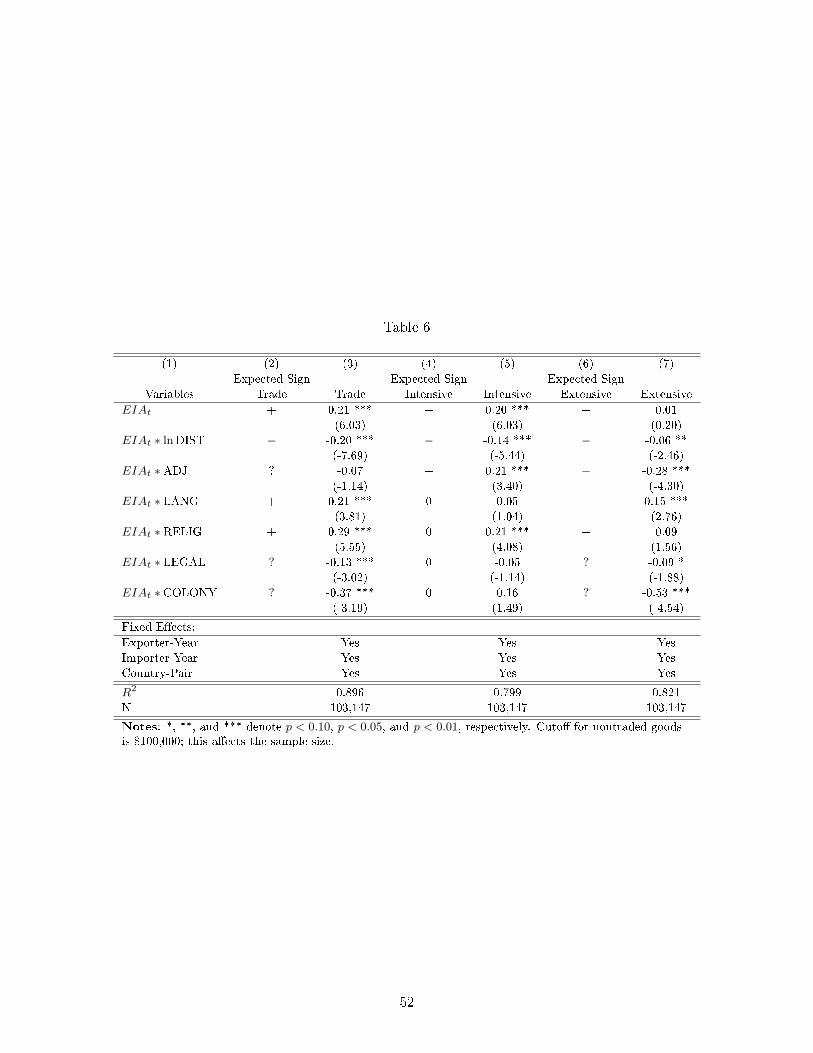
Table 6
(1) (2) (3) (4) (5) (6) (7)
Expected Sign Expected Sign Expected Sign
Variables Trade Trade Intensive Intensive Extensive Extensive
EIAt + 0.21 *** + 0.20 *** + 0.01
(6.03) (6.03) (0.20)
EIAt ∗ lnDIST − -0.20 *** − -0.14 *** − -0.06 **
(-7.69) (-5.44) (-2.46)
EIAt ∗ADJ ? -0.07 + 0.21 *** − -0.28 ***
(-1.14) (3.40) (-4.30)
EIAt ∗ LANG + 0.21 *** 0 0.05 + 0.15 ***
(3.81) (1.04) (2.76)
EIAt ∗ RELIG + 0.29 *** 0 0.21 *** + 0.09
(5.55) (4.08) (1.56)
EIAt ∗ LEGAL ? -0.13 *** 0 -0.05 ? -0.09 *
(-3.02) (-1.14) (-1.88)
EIAt ∗ COLONY ? -0.37 *** 0 0.16 ? -0.53 ***
(-3.19) (1.49) (-4.54)
Fixed Eects:
Exporter-Year Yes Yes Yes
Importer-Year Yes Yes Yes
Country-Pair Yes Yes Yes
R2 0.896 0.799 0.821
N 103,147 103,147 103,147
Notes: *, **, and *** denote p < 0.10, p < 0.05, and p < 0.01, respectively. Cuto for nontraded goodsis $100,000; this aects the sample size.
52
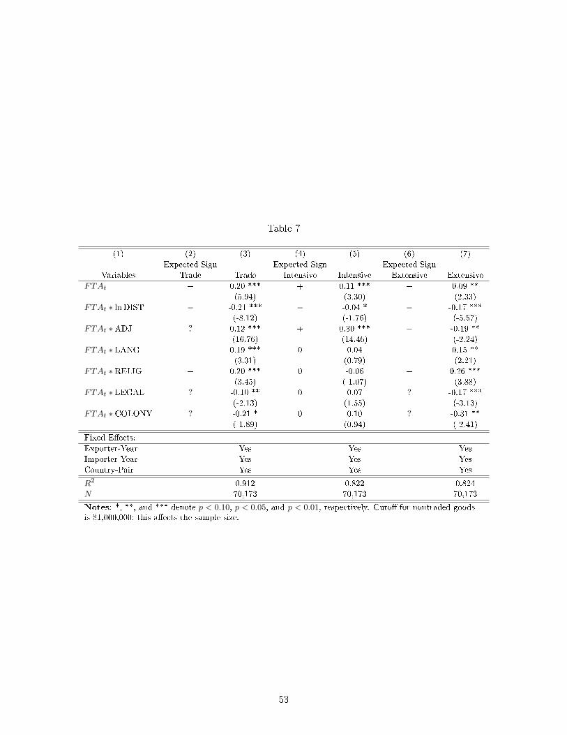
Table 7
(1) (2) (3) (4) (5) (6) (7)
Expected Sign Expected Sign Expected Sign
Variables Trade Trade Intensive Intensive Extensive Extensive
FTAt + 0.20 *** + 0.11 *** + 0.09 **
(5.94) (3.30) (2.33)
FTAt ∗ lnDIST − -0.21 *** − -0.04 * − -0.17 ***
(-8.12) (-1.76) (-5.57)
FTAt ∗ADJ ? 0.12 *** + 0.30 *** − -0.19 **
(16.76) (14.46) (-2.24)
FTAt ∗ LANG + 0.19 *** 0 0.04 + 0.15 **
(3.31) (0.79) (2.21)
FTAt ∗ RELIG + 0.20 *** 0 -0.06 + 0.26 ***
(3.45) (-1.07) (3.88)
FTAt ∗ LEGAL ? -0.10 ** 0 0.07 ? -0.17 ***
(-2.13) (1.55) (-3.13)
FTAt ∗ COLONY ? -0.21 * 0 0.10 ? -0.31 **
(-1.89) (0.94) (-2.41)
Fixed Eects:
Exporter-Year Yes Yes Yes
Importer-Year Yes Yes Yes
Country-Pair Yes Yes Yes
R2 0.912 0.822 0.824
N 70,173 70,173 70,173
Notes: *, **, and *** denote p < 0.10, p < 0.05, and p < 0.01, respectively. Cuto for nontraded goodsis $1,000,000; this aects the sample size.
53
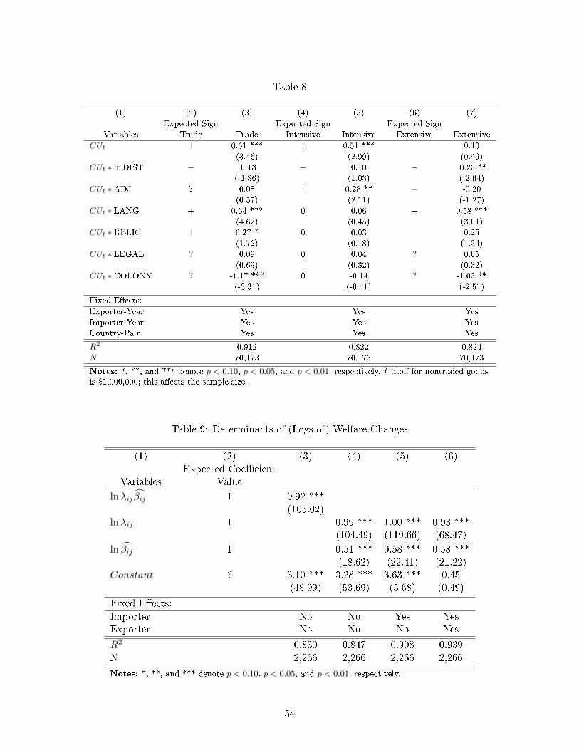
Table 8
(1) (2) (3) (4) (5) (6) (7)
Expected Sign Expected Sign Expected Sign
Variables Trade Trade Intensive Intensive Extensive Extensive
CUt + 0.61 *** + 0.51 *** + 0.10
(3.46) (2.99) (0.49)
CUt ∗ lnDIST − -0.13 − 0.10 − -0.23 **
(-1.36) (1.03) (-2.04)
CUt ∗ADJ ? 0.08 + 0.28 ** − -0.20
(0.57) (2.11) (-1.27)
CUt ∗ LANG + 0.64 *** 0 0.06 + 0.58 ***
(4.62) (0.45) (3.61)
CUt ∗ RELIG + 0.27 * 0 0.03 + 0.25
(1.72) (0.18) (1.34)
CUt ∗ LEGAL ? 0.09 0 0.04 ? 0.05
(0.69) (0.32) (0.32)
CUt ∗ COLONY ? -1.17 *** 0 -0.14 ? -1.03 **
(-3.31) (-0.41) (-2.51)
Fixed Eects:
Exporter-Year Yes Yes Yes
Importer-Year Yes Yes Yes
Country-Pair Yes Yes Yes
R2 0.912 0.822 0.824
N 70,173 70,173 70,173
Notes: *, **, and *** denote p < 0.10, p < 0.05, and p < 0.01, respectively. Cuto for nontraded goodsis $1,000,000; this aects the sample size.
Table 9: Determinants of (Logs of) Welfare Changes
(1) (2) (3) (4) (5) (6)Expected Coecient
Variables Value
lnλij βij 1 0.92 ***(105.02)
lnλij 1 0.99 *** 1.00 *** 0.93 ***(104.49) (119.66) (68.47)
ln βij 1 0.51 *** 0.58 *** 0.58 ***(18.62) (22.41) (21.22)
Constant ? 3.10 *** 3.28 *** 3.63 *** 0.45(48.99) (53.69) (5.68) (0.49)
Fixed Eects:
Importer No No Yes YesExporter No No No Yes
R2 0.830 0.847 0.908 0.939N 2,266 2,266 2,266 2,266
Notes: *, **, and *** denote p < 0.10, p < 0.05, and p < 0.01, respectively.
54
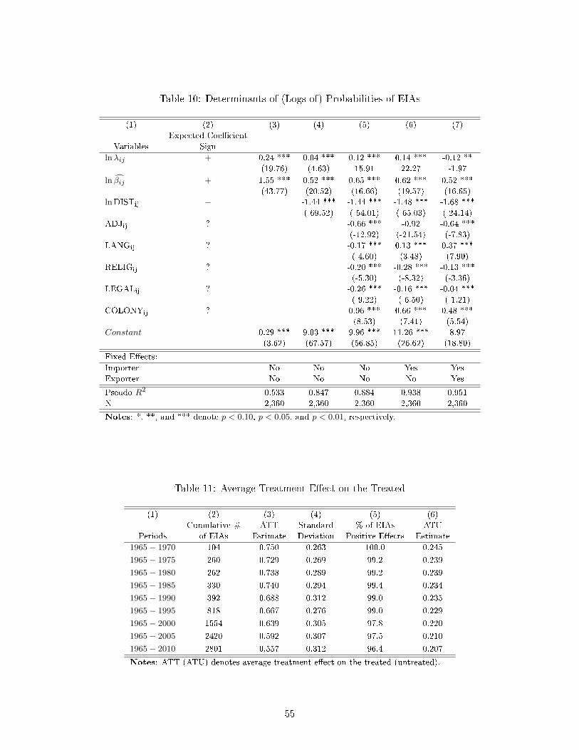
Table 10: Determinants of (Logs of) Probabilities of EIAs
(1) (2) (3) (4) (5) (6) (7)
Expected Coecient
Variables Sign
lnλij + 0.24 *** 0.04 *** 0.12 *** 0.14 *** -0.12 **
(19.76) (4.63) 15.91 22.27 -1.97
ln βij + 1.55 *** 0.52 *** 0.65 *** 0.62 *** 0.52 ***
(43.77) (20.52) (16.66) (19.57) (16.65)
lnDISTij − -1.44 *** -1.44 *** -1.48 *** -1.68 ***
(-69.52) (-54.01) (-65.03) (-24.14)
ADJij ? -0.66 *** -0.92 -0.64 ***
(-12.92) (-21.54) (-7.83)
LANGij ? -0.17 *** 0.13 *** 0.37 ***
(-4.60) (3.48) (7.90)
RELIGij ? -0.20 *** -0.28 *** -0.13 ***
(-5.30) (-8.32) (-3.36)
LEGALij ? -0.26 *** -0.16 *** -0.04 ***
(-9.22) (-6.50) (-1.21)
COLONYij ? 0.96 *** 0.66 *** 0.48 ***
(8.53) (7.41) (5.54)
Constant 0.29 *** 9.03 *** 9.96 *** 11.26 *** 8.97
(3.62) (67.57) (56.85) (26.62) (18.80)
Fixed Eects:
Importer No No No Yes Yes
Exporter No No No No Yes
Pseudo R2 0.533 0.847 0.884 0.938 0.951
N 2,360 2,360 2,360 2,360 2,360
Notes: *, **, and *** denote p < 0.10, p < 0.05, and p < 0.01, respectively.
Table 11: Average Treatment Eect on the Treated
(1) (2) (3) (4) (5) (6)
Cumulative # ATT Standard % of EIAs ATU
Periods of EIAs Estimate Deviation Positive Eects Estimate
1965− 1970 104 0.750 0.263 100.0 0.245
1965− 1975 260 0.729 0.269 99.2 0.239
1965− 1980 262 0.738 0.289 99.2 0.239
1965− 1985 330 0.740 0.294 99.4 0.234
1965− 1990 392 0.688 0.312 99.0 0.235
1965− 1995 818 0.667 0.276 99.0 0.229
1965− 2000 1554 0.639 0.305 97.8 0.220
1965− 2005 2420 0.592 0.307 97.5 0.210
1965− 2010 2801 0.557 0.312 96.4 0.207
Notes: ATT (ATU) denotes average treatment eect on the treated (untreated).
55
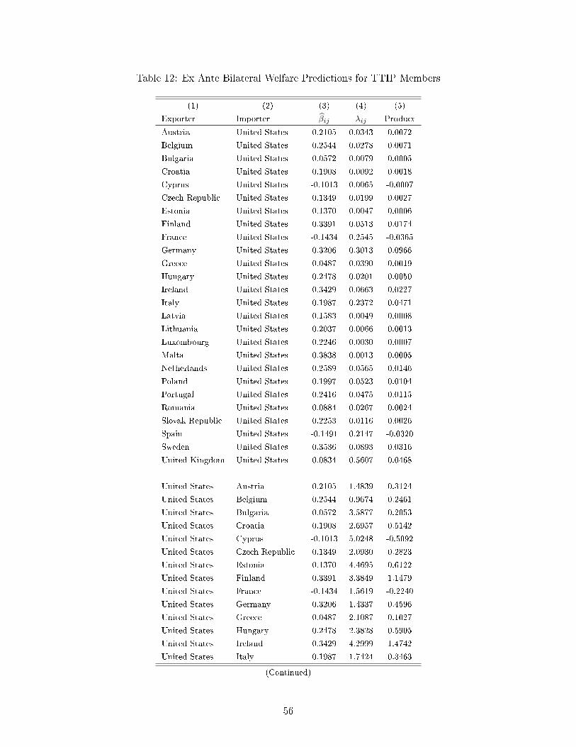
Table 12: Ex Ante Bilateral Welfare Predictions for TTIP Members
(1) (2) (3) (4) (5)
Exporter Importer βij λij Product
Austria United States 0.2105 0.0343 0.0072
Belgium United States 0.2544 0.0278 0.0071
Bulgaria United States 0.0572 0.0079 0.0005
Croatia United States 0.1908 0.0092 0.0018
Cyprus United States -0.1013 0.0065 -0.0007
Czech Republic United States 0.1349 0.0199 0.0027
Estonia United States 0.1370 0.0047 0.0006
Finland United States 0.3391 0.0513 0.0174
France United States -0.1434 0.2545 -0.0365
Germany United States 0.3206 0.3013 0.0966
Greece United States 0.0487 0.0390 0.0019
Hungary United States 0.2478 0.0201 0.0050
Ireland United States 0.3429 0.0663 0.0227
Italy United States 0.1987 0.2372 0.0471
Latvia United States 0.1583 0.0049 0.0008
Lithuania United States 0.2037 0.0066 0.0013
Luxembourg United States 0.2246 0.0030 0.0007
Malta United States 0.3838 0.0013 0.0005
Netherlands United States 0.2589 0.0565 0.0146
Poland United States 0.1997 0.0523 0.0104
Portugal United States 0.2416 0.0475 0.0115
Romania United States 0.0884 0.0267 0.0024
Slovak Republic United States 0.2253 0.0116 0.0026
Spain United States -0.1491 0.2147 -0.0320
Sweden United States 0.3536 0.0893 0.0316
United Kingdom United States 0.0834 0.5607 0.0468
United States Austria 0.2105 1.4839 0.3124
United States Belgium 0.2544 0.9674 0.2461
United States Bulgaria 0.0572 3.5877 0.2053
United States Croatia 0.1908 2.6957 0.5142
United States Cyprus -0.1013 5.0248 -0.5092
United States Czech Republic 0.1349 2.0930 0.2823
United States Estonia 0.1370 4.4695 0.6122
United States Finland 0.3391 3.3849 1.1479
United States France -0.1434 1.5619 -0.2240
United States Germany 0.3206 1.4337 0.4596
United States Greece 0.0487 2.1087 0.1027
United States Hungary 0.2478 2.3828 0.5905
United States Ireland 0.3429 4.2999 1.4742
United States Italy 0.1987 1.7424 0.3463
(Continued)
56
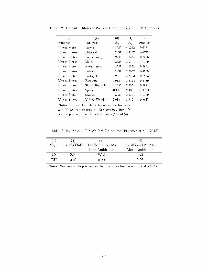
Table 12: Ex Ante Bilateral Welfare Predictions for TTIP Members
(1) (2) (3) (4) (5)
Exporter Importer βij λij Product
United States Latvia 0.1583 4.0242 0.6371
United States Lithuania 0.2037 3.3237 0.6771
United States Luxembourg 0.2246 1.0534 0.2366
United States Malta 0.3838 2.9101 1.1170
United States Netherlands 0.2589 1.1593 0.3002
United States Poland 0.1997 2.2552 0.4503
United States Portugal 0.2416 3.2423 0.7833
United States Romania 0.0884 3.5272 0.3119
United States Slovak Republic 0.2253 2.2554 0.5081
United States Spain -0.1491 2.4891 -0.3711
United States Sweden 0.3536 3.1561 1.1160
United States United Kingdom 0.0834 3.2201 0.2687
Notes: See text for details. Numbers in columns (4)
and (5) are in percentages. Numbers in column (5)
are the product of numbers in columns (3) and (4).
Table 13: Ex Ante TTIP Welfare Gains from Francois et al. (2013)
(1) (2) (3) (4)Region Taris Only Taris and NTMs Taris and NTMs
Less Ambitious More Ambitious
US 0.03 0.12 0.22
EU 0.09 0.20 0.36
Notes: Numbers are in percentages. Estimates are from Francois et al. (2013).
57
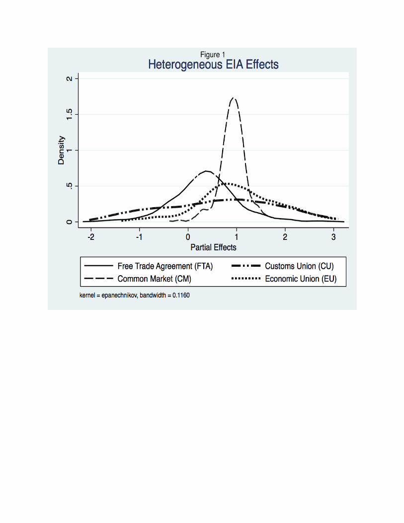
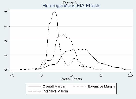
01
23
4
-.5 0 .5 1 1.5Partial Effects
Overall Margin Extensive MarginIntensive Margin
Heterogeneous EIA EffectsFigure 2
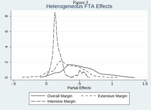
02
46
8
-.5 0 .5 1 1.5Partial Effects
Overall Margin Extensive MarginIntensive Margin
Heterogeneous FTA EffectsFigure 3
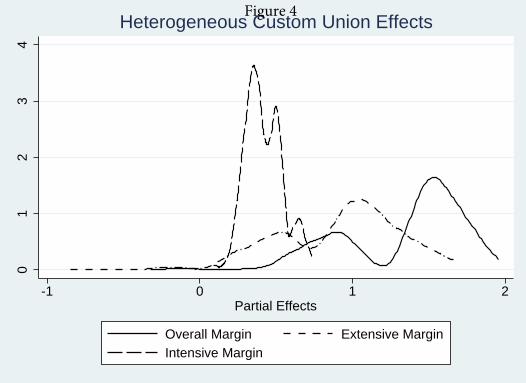
01
23
4
-1 0 1 2Partial Effects
Overall Margin Extensive MarginIntensive Margin
Heterogeneous Custom Union EffectsFigure 4
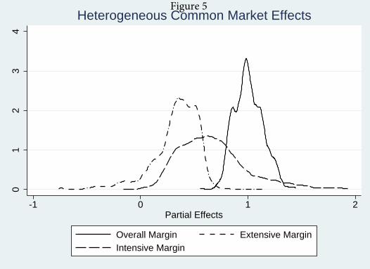
01
23
4
-1 0 1 2Partial Effects
Overall Margin Extensive MarginIntensive Margin
Heterogeneous Common Market EffectsFigure 5
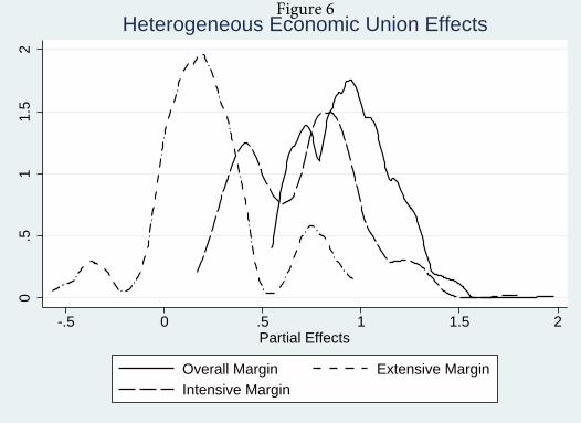
0.5
11.
52
-.5 0 .5 1 1.5 2Partial Effects
Overall Margin Extensive MarginIntensive Margin
Heterogeneous Economic Union EffectsFigure 6
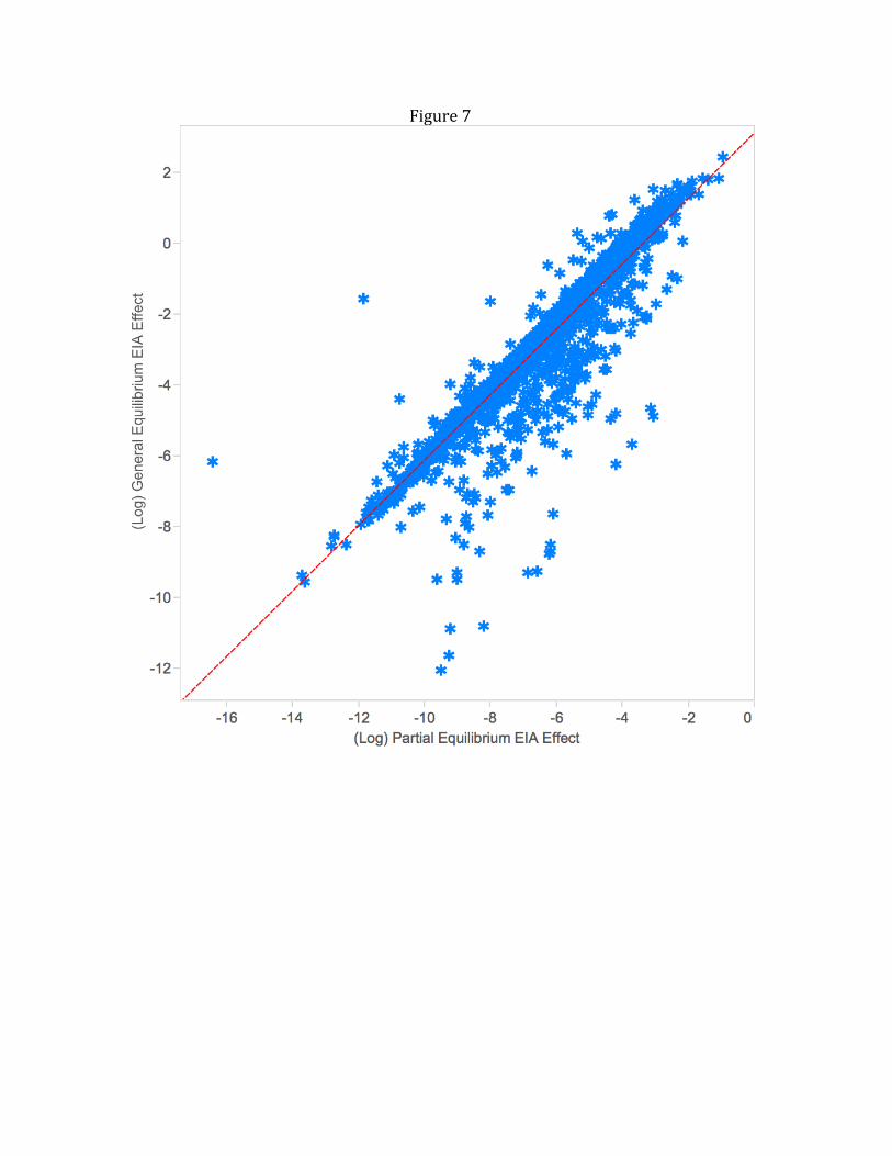
Figure 7
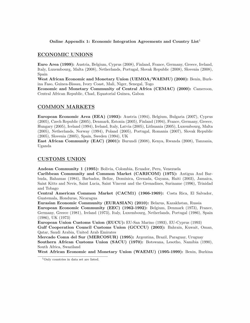
Online Appendix 1: Economic Integration Agreements and Country List1
ECONOMIC UNIONS
Euro Area (1999): Austria, Belgium, Cyprus (2008), Finland, France, Germany, Greece, Ireland,Italy, Luxembourg, Malta (2008), Netherlands, Portugal, Slovak Republic (2008), Slovenia (2008),SpainWest African Economic and Monetary Union (UEMOA/WAEMU) (2000): Benin, Burk-ina Faso, Guinea-Bissau, Ivory Coast, Mali, Niger, Senegal, TogoEconomic and Monetary Community of Central Africa (CEMAC) (2000): Cameroon,Central African Republic, Chad, Equatorial Guinea, Gabon
COMMON MARKETS
European Economic Area (EEA) (1993): Austria (1994), Belgium, Bulgaria (2007), Cyprus(2005), Czech Republic (2005), Denmark, Estonia (2005), Finland (1994), France, Germany, Greece,Hungary (2005), Iceland (1994), Ireland, Italy, Latvia (2005), Lithuania (2005), Luxembourg, Malta(2005), Netherlands, Norway (1994), Poland (2005), Portugal, Romania (2007), Slovak Republic(2005), Slovenia (2005), Spain, Sweden (1994), UKEast African Community (EAC) (2001): Burundi (2008), Kenya, Rwanda (2008), Tanzania,Uganda
CUSTOMS UNION
Andean Community 1 (1995): Bolivia, Colombia, Ecuador, Peru, VenezuelaCaribbean Community and Common Market (CARICOM) (1975): Antigua And Bar-buda, Bahamas (1984), Barbados, Belize, Dominica, Grenada, Guyana, Haiti (2003), Jamaica,Saint Kitts and Nevis, Saint Lucia, Saint Vincent and the Grenadines, Suriname (1996), Trinidadand TobagoCentral American Common Market (CACM1) (1966-1969): Costa Rica, El Salvador,Guatemala, Honduras, NicaraguaEurasian Economic Community (EURASIAN) (2010): Belarus, Kazakhstan, RussiaEuropean Economic Community (EEC) (1962-1992): Belgium, Denmark (1973), France,Germany, Greece (1981), Ireland (1973), Italy, Luxembourg, Netherlands, Portugal (1986), Spain(1986), UK (1973)European Union Customs Union (EUCU): EU-San Marino (1993), EU-Cyprus (1993)Gulf Cooperation Council Customs Union (GCCCU) (2003): Bahrain, Kuwait, Oman,Qatar, Saudi Arabia, United Arab EmiratesMercado Comn del Sur (MERCOSUR) (1995): Argentina, Brazil, Paraguay, UruguaySouthern African Customs Union (SACU) (1970): Botswana, Lesotho, Namibia (1990),South Africa, SwazilandWest African Economic and Monetary Union (WAEMU) (1995-1999): Benin, Burkina
1Only countries in data set are listed.
Faso, Guinea-Bissau (1997), Ivory Coast, Mali, Niger, Senegal, TogoCzech Republic-Slovak Republic (1993-2004)
FREE TRADE AGREEMENTS
I. PLURILATERAL AGREEMENTS
Andean Community 2 (1993-1994): Bolivia, Colombia, Ecuador, VenezuelaArab Common Market (ACM) (1965): Egypt, Iraq, Syria, YemenASEAN-ANZERTA (2010): Australia, New Zealand and ASEAN membersAssociation of Southeast Asian Nations (ASEAN) (2000): Brunei, Cambodia, Indonesia,Laos, Malaysia, Myanmar (Burma), Philippines, Singapore, Thailand, VietnamBaltic FTA (BAFTA 1999-2004): Estonia , Latvia, LithuaniaCaribbean Free Trade Agreement (CARIFTA) (1968-1974): Antigua and Barbuda, Bar-bados, Belize (1971), Dominica, Grenada, Guyana, Jamaica, Saint Kitts and Nevis, Saint Lucia,Saint Vincent and the Grenadines, Trinidad and TobagoCentral American Common Market (CACM2) (1951-1965): Costa Rica (1963), El Sal-vador, Guatemala (1955), Honduras (1957), NicaraguaCentral American Common Market (CACM3) (1993): Costa Rica, El Salvador, Guatemala,Honduras, NicaraguaCentral European Free Trade Area (CEFTA) (1993): Albania (2007), Bosnia and Herze-govina (2007), Bulgaria (1999-2006), Croatia (2003), Czech Republic (until 2004), Hungary (1993-2004), Macedonia (2006), Moldova (2007), Poland (until 2004), Romania (1997-2006), Slovak Re-public (1993-2004), Slovenia (1996-2004)Colombia -Northern Triangle FTA: Colombia, Mexico, El Salvador, Guatemala, HondurasCommon Market for Eastern and Southern Africa (COMESA) (2001): Burundi (2005),Comoros (2006), Congo D.R., Djibouti, Egypt, Eritrea, Ethiopia, Kenya, Libya (2006), Madagas-car, Malawi, Mauritius, Rwanda (2005), Seychelles, Swaziland, Uganda, SudanDominican Republic-Central America-United States FTA (2006) (CAFTA-DR): CostaRica (2009), Dominican Republic (2007), El Salvador, Guatemala (2007), Honduras, Nicaragua,United StatesEuropean Free Trade Association (EFTA 1960): Austria (until 1995), Denmark (until 1973),Finland (1986-1995), Iceland (1970), Norway, Portugal (until 1986), Sweden (until 1995), Switzer-land, United Kingdom (until 1973)European Union (EU) (1958): Austria (1995), Belgium, Bulgaria (2007), Cyprus (2004), CzechRepublic (2004), Denmark (1973), Estonia (2004), Finland (1995), France, Germany, Greece (1981),Hungary (2004), Ireland (1973), Italy, Latvia (2004), Lithuania (2004), Luxembourg, Malta (2004),Netherlands, Poland (2004), Portugal (1986), Slovak Republic (2004), Slovenia (2004), Spain (1986),Sweden (1995), United Kingdom (1973)Gulf Cooperation Council (GCCFTA)(1983-2002): Bahrain, Kuwait, Oman, Qatar, SaudiArabia, United Arab EmiratesNAFTA (North American Free Trade Agreement 1994): Canada, Mexico, USPan-Arab Free Trade Area (1998) (PAFTA/GAFTA): Algeria (2009), Bahrain, Egypt,Iraq, Jordan, Kuwait, Lebanon (1999), Libya (1999), Morocco, Oman, Palestine (2005), Qatar,Saudi Arabia, Sudan (2005), Syria, Tunisia, United Arab Emirates, Yemen (2005)
2
Pacific Island Countries Trade Agreements (2003) (PICTA): Fiji, Kiribati, Papua NewGuinea, Solomon Islands, Tonga, SamoaSouth Asian Free Trade Area (SAFTA)(2006): Bangladesh, Bhutan, India, Maldives, Nepal,Pakistan and Sri LankaSouthern African Development Community (SADC) (2001): Botswana, Congo D.R.,Lesotho, Madagascar, Malawi (2009), Mauritius, Mozambique (2009), Namibia, South Africa,Swaziland, Tanzania (2009), Zambia, ZimbabweTrans-Pacific Partnership (TPP) (2006): Brunei, Chile, New Zealand, SingaporeWest African Monetary Union (WAMU) (1962-1965): Burkina Faso, Mali, Mauritania,Niger, Senegal
II. BILATERAL AGREEMENTS
Albania-Bosnia and Herzegovina (2004-2006)Albania-Croatia (2004-2006)Albania-Macedonia (2003-2006)Albania-Macedonia (2003-2006)Albania-Romania (2004)Andean Community 1-Chile (2005)Andean Community 1-MERCOSUR (2005)Angola-Egypt (2001)Armenia-Georgia (1999)Armenia-Kazakhstan (2002)Armenia-Kyrgyz Republic (1996)Armenia-Moldova (1996)Armenia-Russia (1993)Armenia-Turkmenistan (1997)Armenia-Ukraine (1997)ASEAN-China (2006)ASEAN-India (2010)ASEAN-Japan (2008)ASEAN-South Korea (2007)Australia-Chile (2009)Australia-New Zealand (1983-2009)Australia-Papua New Guinea (1977)Australia-Singapore (2003-2009)Australia-Thailand (2005-2009)Australia-USA (2005)Azerbaijan-Georgia (1997)Azerbaijan-Russia (1993)Azerbaijan-Ukraine (1997)Bahrain-USA (2007)Belarus-Russia (1993-2009)Belarus-Ukraine (2007)Bolivia-Chile (1996-2004)Bolivia-Mexico (1995)
3
Bosnia and Herzegovina-Bulgaria (2005)Bosnia and Herzegovina-Croatia (2001-2006)Bosnia and Herzegovina-Macedonia, (2003-2005)Bosnia and Herzegovina-Moldova (2005-2006)Bosnia and Herzegovina-Romania (2004-2006)Bosnia and Herzegovina-Slovenia (2002-2003)Bulgaria-Israel (2002-2006)Bulgaria-Macedonia (2000-2006)Bulgaria-Moldova (2004)CACM3-Dominican Republic (1998)CACM3-Mexico (2001)Cameroon-Gabon (1966-1999)Canada-Chile (1997)Canada-Israel (1997)Canada-Peru (2010)Canada-USA (1989-1993)CARICOM-Costa Rica (2004)CARICOM-Dominican Republic (1998)CEFTA-Bulgaria (1993-1998)Chile-China (2007)Chile-Costa Rica (2002)Chile-El Salvador (2003)Chile-Japan (2008)Chile-Korea (2004)Chile-Mexico (2000)Chile-Panama (2008)Chile-USA (2004)China-Costa Rica (2010)China-Hong Kong (2004)China-Macao (2004)China-New Zealand (2009)China-Nicaragua (2007)China-Pakistan (2008)China-Peru (2010)Colombia-Mexico (1995-2009)COMESA-SADC (2006)Congo, Republic of-Gabon (1966)Costa Rica-Mexico (1995-2000)Croatia-Macedonia (2004)Czech Republic-Estonia (1997)Czech Republic-Israel (1997-2004)Czech Republic-Latvia (1997-2004)Czech Republic-Lithuania (1997-2004)Czech Republic-Romania (1997-2006)EEC-Israel (1975-1992)EEA-Israel (1993)
4
EFTA-Albania (2010)EFTA-Bulgaria (1994-2006)EFTA-Canada (2010)EFTA-Chile (2005)EFTA-Croatia (2002)EFTA-Czech Republic (1994-2004)EFTA-Egypt (2007)EFTA-Estonia (1997-2004)EFTA-GCCCU (2009)EFTA-Hungary (1994-2004)EFTA-Israel (1993)EFTA-Jordan (2002)EFTA-Latvia (1996-2004)EFTA-Lebanon (2007)EFTA-Lithuania (1997-2004)EFTA-Macedonia (2001)EFTA-Mexico (2002)EFTA-Morocco (2000)EFTA-Poland (1994)EFTA-Romania (1994-2006)EFTA-SACU (2008)EFTA-Singapore (2003)EFTA-Slovak Republic (1993-2004)EFTA-Slovenia (1995-2004)EFTA-South Korea (2007)EFTA-Tunisia (2005)Egypt-Jordan (1999)El Salvador-Panama (2003)Estonia-Hungary (1999-2004)Estonia-Slovak Republic (1997-2004)Estonia-Slovenia (1997-2004)EU-Algeria (2005)EU-Bulgaria (1994-2006)EU-Chile (2005)EU-Croatia (2003)EU-Cyprus (1988-2004)EU-Czech Republic (1992-2004)EU-EFTA (Agreement/European Economic Area 1973/1994)EU-Egypt (2005)EU-Estonia (1998-2004)EU-Faroe Islands (1997)EU-Hungary (1992-2004)EU-Israel (2000)EU-Jordan (2002)EU-Lativa (1995-2004)EU-Lebanon (2003)
5
EU-Lithuania (1995-2004)EU-Macedonia (2002)EU-Mexico (1998)EU-Morocco (2001)EU-Poland (1992-2004)EU-Romania (1993-2006)EU-Slovak Republic (1993-2004)EU-Slovenia (1997-2004)EU-South Africa (2000)EU-Tunisia (1999)Faroe Islands-Iceland (1994)Faroe Islands-Norway (1994)Faroe Islands-Poland (2000-2004)Faroe Islands-Switzerland (1996)Georgia-Kazakhstan (2000)Georgia-Russia (1993)Georgia-Turkmenistan (2000)Georgia-Ukraine (1997)Hungary-Israel (1998-2004)Hungary-Latvia (2000-2004)Hungary-Lithuania (2000-2004)India-Sri Lanka (1999-2005)India-Singapore (2006)India-South Korea (2010)Ireland-Latvia (1995)Ireland-Lithuania (1995)Israel-Mexico (2001)Israel-Poland (1998-2004)Israel-Romania (2002-2006)Israel-Slovak Republic (1997-2004)Israel-Slovenia (1999-2004)Israel-USA (1986)Japan-Switzerland (2010)Jordan-Singapore (2006)Jordan-USA (2002)Kazakhstan-Kyrgyz Republic (1996)Kazakhstan-Russia (1993-2009)Kyrgyz Republic-Moldova (1997)Kyrgyz Republic-Russia (1993)Kyrgyz Republic-Ukraine (1998)Kyrgyz Republic-Uzbekistan (1999-2007)Latvia-Slovak Republic (1997-2004)Lithuania-Poland (1997-2004)Lithuania-Slovak Republic (1997-2004)Lithuania-Slovenia (1997-2003)Macedonia-Moldova (2005-2006)
6
Macedonia-Romania (2004-2006)Macedonia-Slovenia (1997-2003)Macedonia-Ukraine (2002-2005)MERCOSUR-Bolivia (1996-2004)MERCOSUR-Chile (1996)MERCOSUR-Israel (2008)Mexico-Colombia (1995)Mexico-Japan (2005)Mexico-Nicaragua (1999)Mexico-Uruguay (2005)Mexico-Venezuela (1995)Moldova-Ukraine (2005)Morocco-USA (2006)New Zealand-Singapore (2001-2009)New Zealand-Thailand (2006-2009)Oman-USA (2009)Pakistan-Sri Lanka (2005)Panama-Singapore (2007)Peru-Singapore (2010)Peru-USA (2009)Poland-Latvia (1999-2004)Romania-Moldova (1995-2006)Russia-Tajikistan (1993)Russia-Turkmenistan (1993)Russia-Ukraine (1994)Russia-Uzbekistan (1993)SADC-SACU (2009)Slovak Republic-Estonia (1997)Slovenia-Israel (1999)Slovenia-Latvia (1997)Tajikistan-Ukraine (1995)Turkmenistan-Ukraine (1995)TPP-China (2007)Ukraine-Estonia (1997)Ukraine-Uzbekistan (1996)USA-Singapore (2004)
7
Country ListAfghanistan Djibouti Kuwait QatarAlbania Dominica Kyrgyz Republic RomaniaAlgeria Dominican Republic Laos Russian FederationAngola Ecuador Latvia RwandaAntigua And Barbuda Egypt, Arab Rep. Lebanon SamoaArgentina El Salvador Lesotho San MarinoArmenia Equatorial Guinea Liberia Sao Tome and PrincipeAustralia Eritrea Libya Saudi ArabiaAustria Estonia Lithuania SenegalAzerbaijan Ethiopia Luxembourg SeychellesBahamas Faeroe Islands Macao SingaporeBahrain Fiji Macedonia, FYR Slovak RepublicBangladesh Finland Madagascar SloveniaBarbados France Malawi Solomon IslandsBelarus Gabon Malaysia SomaliaBelgium Gambia Maldives South AfricaBelize Georgia Mali SpainBenin Germany Malta Sri LankaBermuda Ghana Marshall Islands St. Kitts and NevisBhutan Greece Mauritania St. LuciaBolivia Greenland Mauritius St. Vincent and the GrenadinesBosnia and Herzegovina Grenada Mexico SudanBotswana Guatemala Micronesia SurinameBrazil Guinea Moldova SwazilandBrunei Darussalam Guinea-Bissau Mongolia SwedenBulgaria Guyana Morocco SwitzerlandBurkina Faso Haiti Mozambique Syrian Arab RepublicBurundi Honduras Myanmar (Burma) TajikistanCambodia Hong Kong Namibia TanzaniaCameroon Hungary Nepal ThailandCanada Iceland Netherlands TogoCape Verde India New Caledonia TongaCayman Islands Indonesia New Zealand Trinidad And TobagoCentral African Republic Iran, Islamic Rep. Nicaragua TunisiaChad Iraq Niger TurkmenistanChile Ireland Nigeria UgandaChina Israel Norway UkraineColombia Italy Oman United Arab EmiratesComoros Ivory Coast Pakistan United KingdomCongo, Dem. Rep. Jamaica Panama United StatesCosta Rica Japan Papua New Guinea UruguayCroatia Jordan Paraguay UzbekistanCuba Kazakhstan Peru VenezuelaCyprus Kenya Philippines VietnamCzech Republic Kiribati Poland YemenDenmark Korea, Rep. Portugal
8
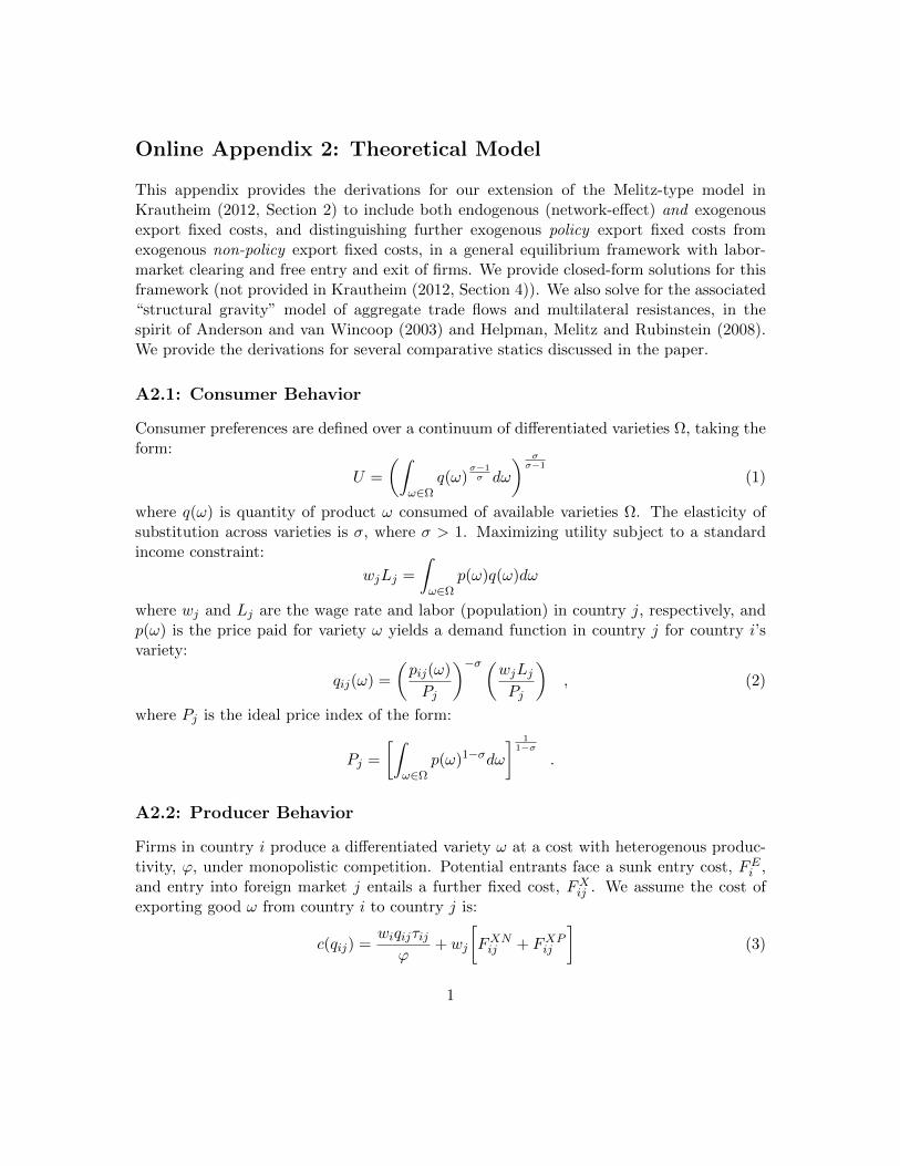
Online Appendix 2: Theoretical Model
This appendix provides the derivations for our extension of the Melitz-type model inKrautheim (2012, Section 2) to include both endogenous (network-effect) and exogenousexport fixed costs, and distinguishing further exogenous policy export fixed costs fromexogenous non-policy export fixed costs, in a general equilibrium framework with labor-market clearing and free entry and exit of firms. We provide closed-form solutions for thisframework (not provided in Krautheim (2012, Section 4)). We also solve for the associated“structural gravity” model of aggregate trade flows and multilateral resistances, in thespirit of Anderson and van Wincoop (2003) and Helpman, Melitz and Rubinstein (2008).We provide the derivations for several comparative statics discussed in the paper.
A2.1: Consumer Behavior
Consumer preferences are defined over a continuum of differentiated varieties Ω, taking theform:
U =
(ˆω∈Ω
q(ω)σ−1σ dω
) σσ−1
(1)
where q(ω) is quantity of product ω consumed of available varieties Ω. The elasticity ofsubstitution across varieties is σ, where σ > 1. Maximizing utility subject to a standardincome constraint:
wjLj =
ˆω∈Ω
p(ω)q(ω)dω
where wj and Lj are the wage rate and labor (population) in country j, respectively, andp(ω) is the price paid for variety ω yields a demand function in country j for country i’svariety:
qij(ω) =
(pij(ω)
Pj
)−σ (wjLjPj
), (2)
where Pj is the ideal price index of the form:
Pj =
[ˆω∈Ω
p(ω)1−σdω
] 11−σ
.
A2.2: Producer Behavior
Firms in country i produce a differentiated variety ω at a cost with heterogenous produc-tivity, ϕ, under monopolistic competition. Potential entrants face a sunk entry cost, FEi ,and entry into foreign market j entails a further fixed cost, FXij . We assume the cost ofexporting good ω from country i to country j is:
c(qij) =wiqijτijϕ
+ wj
[FXNij + FXPij
](3)
1
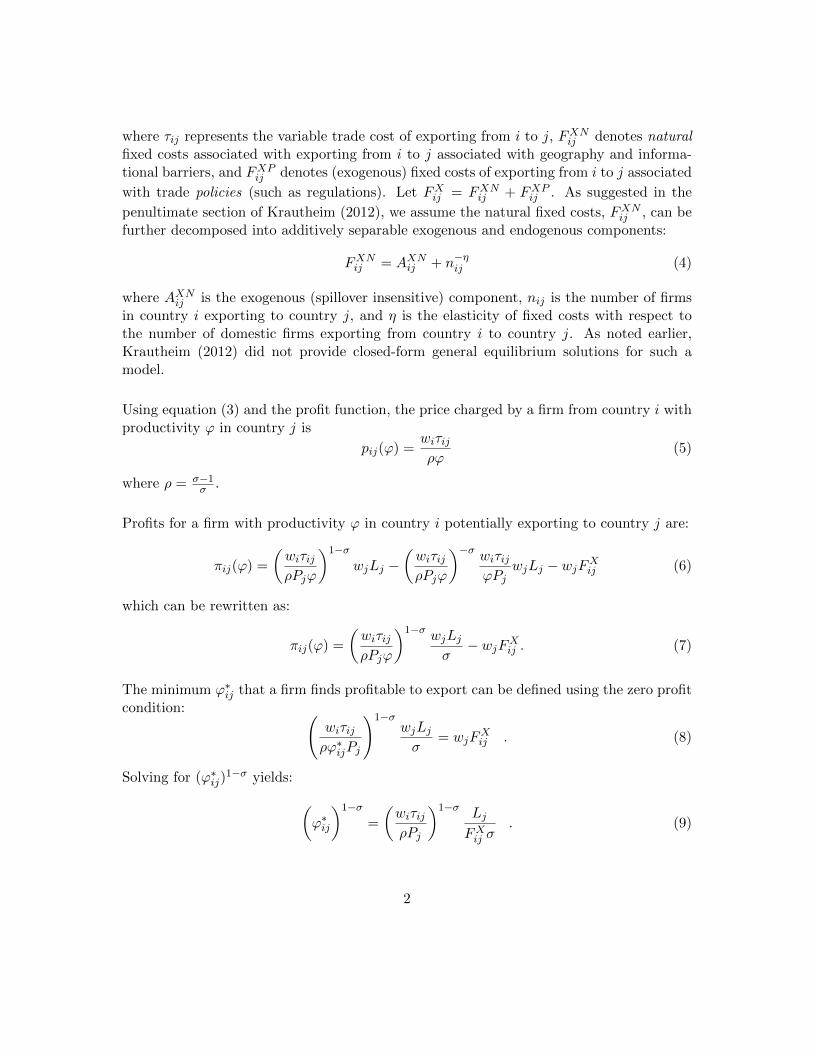
where τij represents the variable trade cost of exporting from i to j, FXNij denotes naturalfixed costs associated with exporting from i to j associated with geography and informa-tional barriers, and FXPij denotes (exogenous) fixed costs of exporting from i to j associated
with trade policies (such as regulations). Let FXij = FXNij + FXPij . As suggested in the
penultimate section of Krautheim (2012), we assume the natural fixed costs, FXNij , can befurther decomposed into additively separable exogenous and endogenous components:
FXNij = AXNij + n−ηij (4)
where AXNij is the exogenous (spillover insensitive) component, nij is the number of firmsin country i exporting to country j, and η is the elasticity of fixed costs with respect tothe number of domestic firms exporting from country i to country j. As noted earlier,Krautheim (2012) did not provide closed-form general equilibrium solutions for such amodel.
Using equation (3) and the profit function, the price charged by a firm from country i withproductivity ϕ in country j is
pij(ϕ) =wiτijρϕ
(5)
where ρ = σ−1σ .
Profits for a firm with productivity ϕ in country i potentially exporting to country j are:
πij(ϕ) =
(wiτijρPjϕ
)1−σwjLj −
(wiτijρPjϕ
)−σ wiτijϕPj
wjLj − wjFXij (6)
which can be rewritten as:
πij(ϕ) =
(wiτijρPjϕ
)1−σ wjLjσ− wjFXij . (7)
The minimum ϕ∗ij that a firm finds profitable to export can be defined using the zero profitcondition: (
wiτijρϕ∗ijPj
)1−σwjLjσ
= wjFXij . (8)
Solving for (ϕ∗ij)1−σ yields: (
ϕ∗ij
)1−σ=
(wiτijρPj
)1−σ Lj
FXij σ. (9)
2
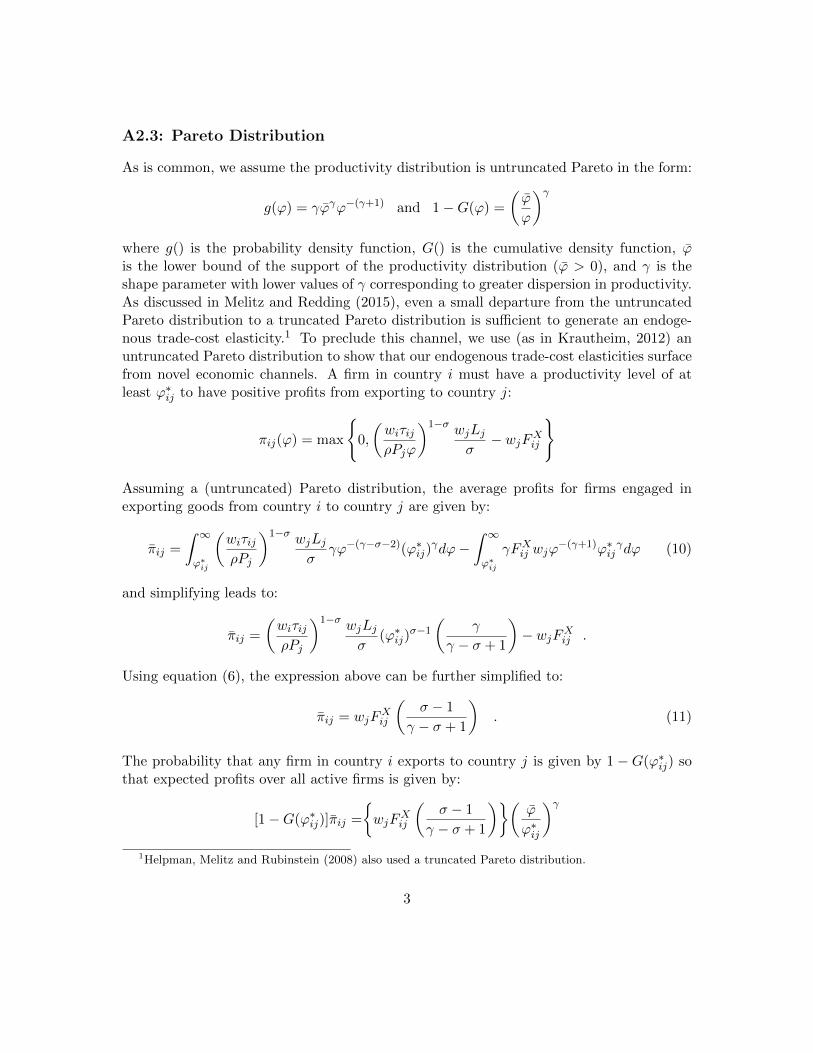
A2.3: Pareto Distribution
As is common, we assume the productivity distribution is untruncated Pareto in the form:
g(ϕ) = γϕγϕ−(γ+1) and 1−G(ϕ) =
(ϕ
ϕ
)γwhere g() is the probability density function, G() is the cumulative density function, ϕis the lower bound of the support of the productivity distribution (ϕ > 0), and γ is theshape parameter with lower values of γ corresponding to greater dispersion in productivity.As discussed in Melitz and Redding (2015), even a small departure from the untruncatedPareto distribution to a truncated Pareto distribution is sufficient to generate an endoge-nous trade-cost elasticity.1 To preclude this channel, we use (as in Krautheim, 2012) anuntruncated Pareto distribution to show that our endogenous trade-cost elasticities surfacefrom novel economic channels. A firm in country i must have a productivity level of atleast ϕ∗ij to have positive profits from exporting to country j:
πij(ϕ) = max
0,
(wiτijρPjϕ
)1−σ wjLjσ− wjFXij
Assuming a (untruncated) Pareto distribution, the average profits for firms engaged inexporting goods from country i to country j are given by:
πij =
ˆ ∞ϕ∗ij
(wiτijρPj
)1−σ wjLjσ
γϕ−(γ−σ−2)(ϕ∗ij)γdϕ−
ˆ ∞ϕ∗ij
γFXij wjϕ−(γ+1)ϕ∗ij
γdϕ (10)
and simplifying leads to:
πij =
(wiτijρPj
)1−σ wjLjσ
(ϕ∗ij)σ−1
(γ
γ − σ + 1
)− wjFXij .
Using equation (6), the expression above can be further simplified to:
πij = wjFXij
(σ − 1
γ − σ + 1
). (11)
The probability that any firm in country i exports to country j is given by 1 −G(ϕ∗ij) sothat expected profits over all active firms is given by:
[1−G(ϕ∗ij)]πij =
wjF
Xij
(σ − 1
γ − σ + 1
)(ϕ
ϕ∗ij
)γ1Helpman, Melitz and Rubinstein (2008) also used a truncated Pareto distribution.
3
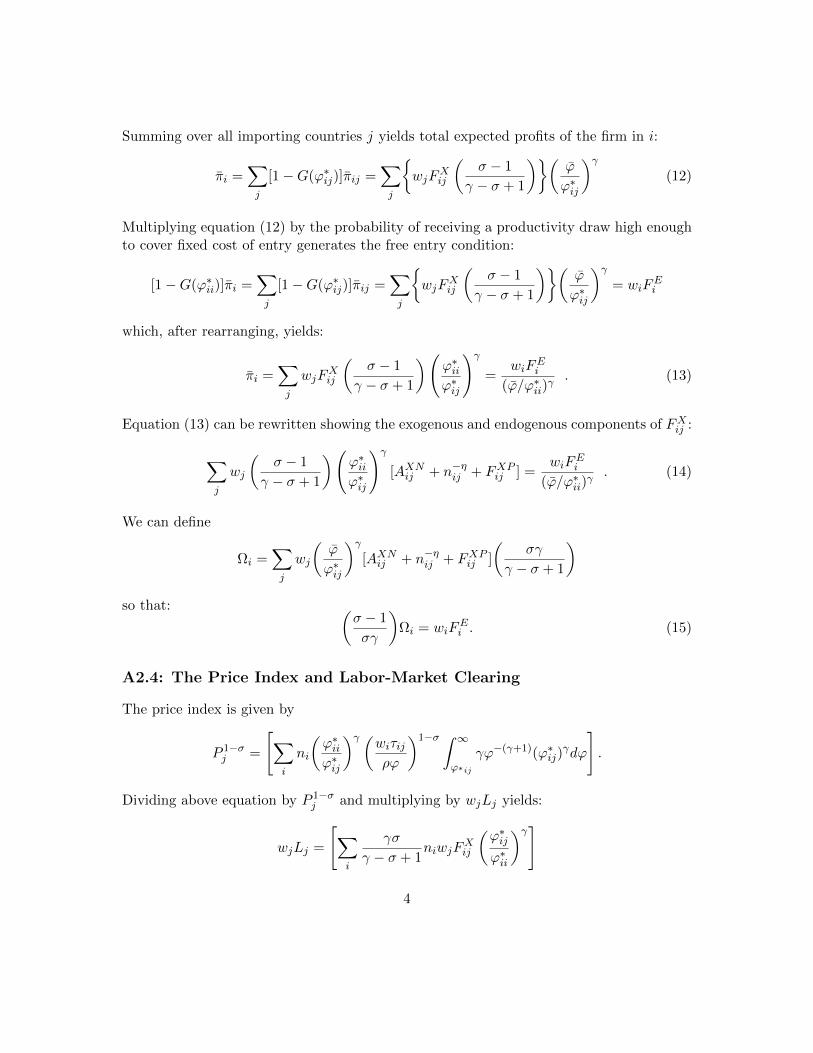
Summing over all importing countries j yields total expected profits of the firm in i:
πi =∑j
[1−G(ϕ∗ij)]πij =∑j
wjF
Xij
(σ − 1
γ − σ + 1
)(ϕ
ϕ∗ij
)γ(12)
Multiplying equation (12) by the probability of receiving a productivity draw high enoughto cover fixed cost of entry generates the free entry condition:
[1−G(ϕ∗ii)]πi =∑j
[1−G(ϕ∗ij)]πij =∑j
wjF
Xij
(σ − 1
γ − σ + 1
)(ϕ
ϕ∗ij
)γ= wiF
Ei
which, after rearranging, yields:
πi =∑j
wjFXij
(σ − 1
γ − σ + 1
)(ϕ∗iiϕ∗ij
)γ=
wiFEi
(ϕ/ϕ∗ii)γ. (13)
Equation (13) can be rewritten showing the exogenous and endogenous components of FXij :
∑j
wj
(σ − 1
γ − σ + 1
)(ϕ∗iiϕ∗ij
)γ[AXNij + n−ηij + FXPij ] =
wiFEi
(ϕ/ϕ∗ii)γ. (14)
We can define
Ωi =∑j
wj
(ϕ
ϕ∗ij
)γ[AXNij + n−ηij + FXPij ]
(σγ
γ − σ + 1
)so that: (
σ − 1
σγ
)Ωi = wiF
Ei . (15)
A2.4: The Price Index and Labor-Market Clearing
The price index is given by
P 1−σj =
[∑i
ni
(ϕ∗iiϕ∗ij
)γ (wiτijρϕ
)1−σ ˆ ∞ϕ∗ij
γϕ−(γ+1)(ϕ∗ij)γdϕ
].
Dividing above equation by P 1−σj and multiplying by wjLj yields:
wjLj =
[∑i
γσ
γ − σ + 1niwjF
Xij
(ϕ∗ijϕ∗ii
)γ]
4
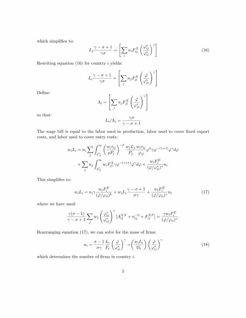
which simplifies to:
Ljγ − σ + 1
γσ=
[∑i
niFXij
(ϕ∗ijϕ∗ii
)γ](16)
Rewriting equation (16) for country i yields:
Liγ − σ + 1
γσ=
∑j
njFXji
(ϕ
ϕ∗ji
)γDefine:
Λi =
∑j
njFXji
(ϕ
ϕ∗ji
)γso that:
Li/Λi =γσ
γ − σ + 1
The wage bill is equal to the labor used in production, labor used to cover fixed exportcosts, and labor used to cover entry costs:
wiLi = ni∑j
ˆ ∞ϕ∗ij
(wiτijρPj
)−σ wjLjPj
wiτijϕij
ϕσγϕ−(γ+1)ϕγdϕ
+∑j
nj
ˆ ∞ϕ∗ij
wiFXji γϕ
−(γ+1)ϕγdϕ+wiF
Ei
(ϕ/ϕ∗ii)γni
This simplifies to:
wiLi = niγwiF
Ei
(ϕ/ϕii)k+ wiLi
γ − σ + 1
σγ+
wiFEi
(ϕ/ϕii)γni (17)
where we have used:
γ(σ − 1)
γ − σ + 1
∑j
wj
(ϕ∗iiϕ∗ij
)γ[AXNij + n−ηij + FXPij ] =
γwiFEi
(ϕ/ϕii)γ.
Rearranging equation (17), we can solve for the mass of firms:
ni =σ − 1
σγ
LiFe
(ϕ
ϕ∗ii
)γ=
(wiLiΩi
)(ϕ
ϕ∗ii
)γ(18)
which determines the number of firms in country i.
5
The probability that a firm in country i exports to j is given by:
1−G(ϕ∗ij)
1−G(ϕ∗ii)= ζij where 1−G(ϕ∗ij) =
(ϕ
ϕ∗ij
)γ.
Consequently:
nij = ζijni
=
(ϕϕ∗ij
)γ(
ϕϕ∗ii
)γ σ − 1
σγ
Li
FEi
(ϕ
ϕ∗ii
)γ
=σ − 1
γσFEiLi
(ϕ
ϕ∗ij
)γ. (19)
Hence, the number of firms in country i exporting to country j depends on the cut-offproductivity. We can rewrite equation (19) as:
nij = δi(ϕ∗ij/ϕ)−γ (20)
where δi is a country specific scaling factor:
δi =σ − 1
γσFEiLi. (21)
A2.5: Structural Gravity for Trade Flows
We can provide a structural gravity representation of aggregate trade flows. The tradeflow from country i to country j is:
Xij = nij
ˆ ∞ϕ∗ij
(wiτijρPj
)1−σ wjLjσ
σγϕ−(γ−σ+1)(ϕ∗ij)γdϕ
Simplifying the above equation, using equations (13) and (14), yields:
Xij = nij
(wiτijρPj
)1−σ wjLjσ
(ϕ∗ij/ϕ)σ−1︸ ︷︷ ︸wj(AXNij +δ−ηi (ϕij/ϕ)γη+FXPij )
γσ
γ − σ + 1
so that:
Xij =σ − 1
(γ − σ + 1)FEiLiwj
[(AXNij + FXPij
)(ϕ∗ij/ϕ)−γ + δ−ηi (ϕ∗ij/ϕ)γ(η−1))
]
6
or more succinctly:
Xij =σ − 1
(γ − σ + 1)FEiLi(
ϕ∗ijϕ
)−γwjFXij (22)
where
FXij =
[AXNij + δi((ϕ
∗ij/ϕ)σ−1)
ηγσ−1 + FXPij
].
Summing Xij over all i yields total expenditures for country j:
wjLj = wjγσ
(γ − σ + 1)
∑i
(σ − 1)Li
γσFEi
(ϕ∗ijϕ
)−γFXij
Given the definition of Λj above, this implies:
Lj/Λj =γσ
(γ − σ + 1)
Summing trade flows Xij over all j destination markets for i yields:
wiLi =σ − 1
γσFEiLi∑j
[(ϕ∗ijϕ
)−γwjFXij
γσ
(γ − σ + 1)
]or
wiLi/Ωi =σ − 1
γσFEiLi
Making appropriate substitutions into trade equation (22) yields:
Xij =
(σ − 1
γσFEiLi
)(wj
γσ
(γ − σ + 1)
)([(AXNij + FXPij
)(ϕ∗ij/ϕ)−γ + δ−ηi (ϕ∗ij/ϕ)γ(η−1)
])Appropriate substitutions yields the structural gravity equation:
Xij =
(ϕ∗ij/ϕ)−γ[(AXNij + FXPij
)+ δ−ηi (ϕ∗ij/ϕ)γη
]ΩiΛj
(wiLi)(wjLj) (23)
or
Xij =
((ϕ∗ij/ϕ)−γFXij
ΩiΛj
)(wiLi)(wjLj)
where
Ωi =∑j
wj
(ϕ∗ijϕ
)−γFXij
(σγ
γ − σ + 1
)=∑j
wjLjΛj
FXij
(ϕ∗ijϕ
)−γ
7
and
Λj =∑i
NiFXij
(ϕ∗ijϕ
)−γ=∑i
wiLiΩi
FXij
(ϕ∗ijϕ
)−γwhich is analogous to the structural gravity model in Anderson and van Wincoop (2003).
A2.6: Stability Conditions
Here we show the conditions for existence of the cut-off productivity for exports fromcountry i to country j. The fixed point is given by:(
wiτijρPj
)1−σ wjLjσ
(ϕ∗ij/ϕ)σ−1 = wj
[AXNij + δ−ηi (ϕ∗ij/ϕ)ηγ + FXPij
](24)
We define:
Rij =
(wiτijρPj
)1−σ wjLjσ
(ϕ∗ij/ϕ)σ−1
and
Cij = wj
[AXNij + δ−ηi ((ϕ∗ij/ϕ)σ−1)
ηγσ−1 + FXPij
]Since AXNij + FXPij ≥ 0 (by assumption), there exists a stable cut-off productivity if
∂Cij/∂(ϕ∗ij/ϕ)σ−1 < ∂Rij/∂(ϕ∗ij/ϕ)σ−1 when Cij = Rij . This implies:
γη
(σ − 1)wj
δ−ηi
((ϕ∗ij/ϕ)σ−1
) γησ−1
(ϕ∗ij/ϕ)σ−1<
(wiτijρPj
)1−σ wjLjσ
= (ϕ∗ij/ϕ)1−σwj
[AXNij +δηi ((ϕ∗ij/ϕ)σ−1)
ηγσ−1 +FXPij
]The above equation simplifies to:
γη
σ − 1
δ−ηi
((ϕ∗ij/ϕ)σ−1
) γησ−1
[AXNij + δ−ηi ((ϕ∗ij/ϕ)σ−1)
ηγσ−1 + FXPij
] < 1
If we define:
sij =δ−ηi (ϕ∗ij/ϕ)γη
AXNij + δ−ηi (ϕ∗ij/ϕ)γη + FXPij
the stability condition reduces to:
1 >γ
σ − 1ηsij .
Throughout the next section of comparative statics, we assume 1− γσ−1ηsij > 0. Krautheim
(2012) assumed the same condition, where in his model sij is assumed to be 1; in our model,sij ≤ 1.
8
A2.7: Comparative Statics
It is important to note that we are primarily interested in this section in the comparativestatics associated with “partial effects” of changes in τij and FXPij on Xij . Changes inthese variables have direct partial effects, but also work indirectly through changes in thecutoff productivity, ϕ∗ij . Consequently, it is useful to determine the effects of changes in τijand FXPij on ϕ∗ij . Moreover, we ignore general equilibrium effects on wage rates and prices,e.g., wi and Pj ; the effects on these wage rates and prices are addressed in Section 8 of thepaper, which discusses general equilibrium effects.
Comparative Static 1a
The first comparative static in the paper is the effect of changes in (log) variable tradecosts (d ln τij) on the (log) cutoff productivity for exporting from i to j (d lnϕ∗ij). Startingwith the equation determining the cutoff productivity, equation (24) above, we take thelogarithms of both sides of equation (24) yielding:
(1− σ) lnwi + (1− σ) ln τij + (σ − 1) ln ρ+ (σ − 1) lnPj + lnwj + lnLj
− lnσ + (σ − 1) ln(ϕ∗ij/ϕ) = lnwj + ln[AXNij + δ−ηij (ϕ∗ij/ϕ)ηγ + FXPij ] (25)
Differentiating the equation above yields:
(1− σ)d ln τij + (σ − 1)d lnϕ∗ij =
(δ−ηi ηγ(ϕ∗ij/ϕ)γη
AXNij + δ−ηi (ϕ∗ij/ϕ)γη + FXPij
)d lnϕ∗ij (26)
where d ln ρ = d ln ϕ = d lnLj = dAXNij = dFXPij = 0 by assumption and, as discussedabove, d lnwi = d lnPj = 0. Simplifying the above equation, using the definition of sijnoted above, yields:
[(σ − 1)− γηsij ]d lnϕ∗ij = (σ − 1)d ln τij (27)
or
d lnϕ∗ij =1
1− γσ−1ηsij
d ln τij (28)
We note that, in the case of AXNij = FXPij = 0, sij = 1 and consequently this comparativestatic would be the same as implied by equation (6) in Krautheim (2012).
Comparative Static 1b
Start with structural gravity equation (23):
Xij =
(ϕ∗ij/ϕ)−γ[(AXNij + FXPij
)+ δ−ηi (ϕ∗ij/ϕ)γη
]ΩiΛj
(wiLi)(wjLj) (29)
9
Taking logarithms:
lnXij = ln(wiLi/Ωi)+ln(wjLj/Λj)−γ ln(ϕ∗ij/ϕ)+ln[(AXNij +FXPij )+δ−ηi (ϕ∗ij/ϕ)γη] (30)
Differentiating and solving for the partial (elasticity) effect of a (log) change in ϕ∗ij yields:
d lnXij = −γd lnϕ∗ij +δ−ηi γη(ϕ∗ij/ϕ)γηd lnϕ∗ij
[(AXNij + FXPij ) + δ−ηi (ϕ∗ij/ϕ)γη]
= −γd lnϕ∗ij + γηsijd lnϕ∗ij
= −γ(1− ηsij)d lnϕ∗ij (31)
In Comparative Static 1a, we found that:
d lnϕ∗ij =1
1− γσ−1ηsij
d ln τij . (32)
Hence, Comparative Static 1b is:
d lnXij = −γ(
1− ηsij1− γ
σ−1ηsij
)d ln τij (33)
which, after some algebra, can also be written as:
d lnXij =
[−(σ − 1)−
(γ − (σ − 1)
1− γσ−1ηsij
)]d ln τij . (34)
The form of the equation above suggests that the effect of a change in τij can be decomposedinto intensive and extensive margin effects, which we address below.
Comparative Statics 1c and 1d
We can decompose the change in the aggregate trade flow into changes in the intensive andextensive margins. Aggregate trade can be written as:
Xij = wiLi
ˆ ∞ϕ∗ij
xij(ϕ)dG(ϕ)
Using Leibniz rule to separate the intensive and extensive margins, differentiation withrespect to τij yields:
dXij =
[wiLi
ˆϕ∗ij∞∂xij(ϕ)
∂τijdG(ϕ)
]dτij −
[wiLix(ϕ∗ij)G′(ϕ∗ij)
∂ϕ∗ij∂τij
]dτij (35)
10
The first RHS term is the intensive margin change and the second RHS term is the extensivemargin change.
Comparative Static 1c is the intensive margin elasticity of trade to a one percent changein τij . At ∂ϕ∗ij/∂τij = 0, the elasticity of equilibrium individual exports, xij , to ∂ ln τij is:
∂ lnxij∂ ln τij
=∂xij/xij∂τij/τij
= −(σ − 1)
Integration over all exporters yields:
d ln IMij
d ln τij= −(σ − 1).
Comparative Static 1d is the extensive margin elasticity of trade to a one percent changein τij . Using the definition of the equilibrium productivity threshold, we have:
∂ϕ∗ij∂τij
=ϕ∗
τij
Using equation (35), the extensive margin elasticity with respect to a one percent changein τij is:
d lnEMij
d ln τij=−τijXij
(wiLix(ϕ∗ij)G′(ϕ∗ij)
ϕ∗ijτij
)which, after substitutions, yields:
d lnEMij
d ln τij= −
(γ − (σ − 1)
1− γσ−1ηsij
)
Comparative Static 2a
The next comparative static in the paper is the effect of changes in exogenous policy-oriented export fixed costs, FXPij , on the export cutoff productivity, d lnϕ∗ij . Starting withequation (25) above, differentiating yields:
(σ − 1)d lnϕ∗ij =
(dFXPij + δ−ηi ηγ(ϕ∗ij/ϕ)γηd lnϕ∗ij
AXNij + δ−ηi (ϕ∗ij/ϕ)γη + FXPij
)(36)
where d ln ρ = d ln ϕ = d lnLj = dτij = dAXNij = 0 by assumption and, as discussed above,d lnwi = d lnPj = 0. Simplifying the above equation, using the definition of sij notedabove, yields:
d lnϕ∗ij =
(1
(σ − 1)(1− γσ−1ηsij)
)(FXPij
AXNij + δ−ηi (ϕ∗ij/ϕ)γη + FXPij
)d lnFXPij (37)
11
Given the stability condition for the export cutoff productivity, the first term in largeparentheses on the RHS is positive. Given the second term in large parentheses on theRHS is also positive, it follows that the relationship between d lnϕ∗ij and dFXPij is positive.Note that there is no such comparative static in Krautheim (2012); this also holds for theremaining comparative statics below.
Comparative Static 2b
We now solve explicitly for the effect of a (log) change in policy-based fixed export costson the aggregate trade flow, Start with structural gravity equation (23):
Xij =
(ϕ∗ij/ϕ)−γ[(AXNij + FXPij
)+ δ−ηi (ϕ∗ij/ϕ)γη
]ΩiΛj
(wiLi)(wjLj) (38)
Take the logarithms of both sides of the equation above and differentiate with respect tolnϕ∗ij and with respect to lnFXPij . Incorporating results from (analogous) ComparativeStatic 1b above, we find:
d lnXij = −γ(1− ηsij)d lnϕ∗ij +FXPij
AXNij + δ−ηi (ϕ∗ij/ϕ)γη + FXPij
d lnFXPij . (39)
In Comparative Static 2a, we found:
d lnϕ∗ij =
(1
(σ − 1)(1− γσ−1ηsij)
)(FXPij
AXNij + δ−ηi (ϕ∗ij/ϕ)γη + FXPij
)d lnFXPij (40)
Substitution of the equation above into equation (39) yields:
d lnXij =
[− γ
σ − 1
(1− ηsij
1− γσ−1ηsij
)(FXPij
AXNij + δ−ηi (ϕ∗ij/ϕ)γη + FXPij
)+ 1
]d lnFXPij
With some algebra, this equation can be rewritten as:
d lnXij =
([1
σ − 1
(−(σ − 1)− γ − (σ − 1)
1− γσ−1ηsij
)]+ 1
)(FXPij
AXNij + δ−ηi (ϕ∗ij/ϕ)γη + FXPij
)d lnFXPij
which simplifies to:
d lnXij = −
(γ
σ−1 − 1
1− γσ−1ηsij
)(FXPij
AXNij + δ−ηi (ϕ∗ij/ϕ)γη + FXPij
)d lnFXPij
which is the same as the comparative static in the main paper, since n−ηij = δ−ηi (ϕ∗ij/ϕ)γη.
12
Comparative Statics 2c and 2d
Similar to Comparative Static 1c, we can decompose the change in the aggregate tradeflows into changes in the intensive and extensive margins using Leibniz rule.
Using the definition of the equilibrium firm-level exports, ∂xij(ϕ)/∂FXPij = 0. Conse-
quently, the elasticity of the intensive margin with respect to a one percent change in FXPij
is:d ln IMij
d lnFXPij
= 0. (41)
Using the definition of the equilibrium productivity threshold and the same procedure as inComparative Static 1d, the elasticity of the extensive margin with respect to a one percentchange in FXPij is:
d lnEMij = −
(γ
σ−1 − 1
1− γσ−1ηsij
)(FXPij
AXNij + δ−ηi (ϕ∗ij/ϕ)γη + FXPij
)d lnFXPij
which is the same as d lnXij/d lnFXPij .
Proof
The following derivation proves that d ln(−d lnEMij
d lnFXPij)/dFXPij is positive.
ln
(−dlnEMij
dlnFXPij
)= ln
(γ
σ − 1− 1
)− ln
(1− γ
σ − 1ηsij
)+ lnFXPij − ln
(AXNij + FXPij + n−ηij
)= 0−
(1
1− γσ−1ηsij
)(− γ
σ − 1η
)dsij
dFXPij
+1
FXPij
dFXPij
dFXPij
−
(1
AXNij + FXPij + n−ηij
)dFXPij
dFXPij
=
γσ−1η
1− γσ−1ηsij
dsij
dFXPij
+1
FXPij
− 1
AXNij + FXPij + n−ηij(42)
Remember that:
dsij
dFXPij
=
(AXNij + FXPij + n−ηij
)(0)− n−ηij (1)
(AXNij + FXPij + n−ηij )2
=−n−ηij(
AXNij + FXPij + n−ηij
)2 (43)
13
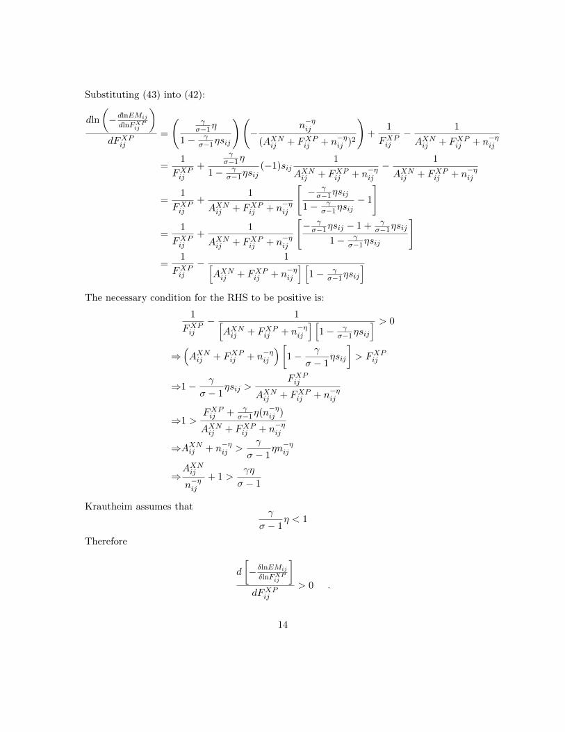
Substituting (43) into (42):
dln
(−dlnEMij
dlnFXPij
)dFXPij
=
(γ
σ−1η
1− γσ−1ηsij
)(−
n−ηij
(AXNij + FXPij + n−ηij )2
)+
1
FXPij
− 1
AXNij + FXPij + n−ηij
=1
FXPij
+
γσ−1η
1− γσ−1ηsij
(−1)sij1
AXNij + FXPij + n−ηij− 1
AXNij + FXPij + n−ηij
=1
FXPij
+1
AXNij + FXPij + n−ηij
[− γσ−1ηsij
1− γσ−1ηsij
− 1
]
=1
FXPij
+1
AXNij + FXPij + n−ηij
[− γσ−1ηsij − 1 + γ
σ−1ηsij
1− γσ−1ηsij
]=
1
FXPij
− 1[AXNij + FXPij + n−ηij
] [1− γ
σ−1ηsij
]The necessary condition for the RHS to be positive is:
1
FXPij
− 1[AXNij + FXPij + n−ηij
] [1− γ
σ−1ηsij
] > 0
⇒(AXNij + FXPij + n−ηij
)[1− γ
σ − 1ηsij
]> FXPij
⇒1− γ
σ − 1ηsij >
FXPij
AXNij + FXPij + n−ηij
⇒1 >FXPij + γ
σ−1η(n−ηij )
AXNij + FXPij + n−ηij
⇒AXNij + n−ηij >γ
σ − 1ηn−ηij
⇒AXNij
n−ηij+ 1 >
γη
σ − 1
Krautheim assumes thatγ
σ − 1η < 1
Therefore
d
[− δlnEMij
δlnFXPij
]dFXPij
> 0 .
14
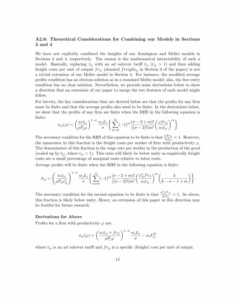
A2.8: Theoretical Considerations for Combining our Models in Sections3 and 4
We have not explicitly combined the insights of our Armington and Melitz models inSections 3 and 4, respectively. The reason is the mathematical intractability of such amodel. Basically, replacing τij with an ad valorem tariff tij (tij > 1) and then addingfreight costs per unit of output frij (denoted freightij in Section 3 of the paper) is nota trivial extension of our Melitz model in Section 4. For instance, the modified averageprofits condition has no obvious solution as in a standard Melitz model; also, the free entrycondition has no clear solution. Nevertheless, we provide some derivations below to showa direction that an extension of our paper to merge the two features of each model mightfollow.
For brevity, the key considerations that are derived below are that the profits for any firmmust be finite and that the average profits also need to be finite. In the derivations below,we show that the profits of any firm are finite when the RHS in the following equation isfinite:
πij(ϕ) =
(witijρPjϕ
)1−σ wjLjσ
∞∑m=0
(−1)m(σ − 2 +m)!
((σ − 2)!)m!
(ϕfrijwitij
)mThe necessary condition for the RHS of this equation to be finite is that
ϕfrijwitij
< 1. However,
the numerator in this fraction is the freight costs per worker of firm with productivity ϕ.The denominator of this fraction is the wage rate per worker in the production of the good(scaled up by tij , where tij > 1). This ratio will likely be below unity as empirically freightcosts are a small percentage of marginal costs relative to labor costs.
Average profits will be finite when the RHS in the following equation is finite:
πij =
(witijρPjϕ∗ij
)1−σwjLjσ
∞∑m=0
(−1)m(σ − 2 +m)!
((σ − 2)!)m!
(ϕ∗ijfrij
witij
)m( k
k − σ − 1 +m
)
The necessary condition for the second equation to be finite is thatϕ∗ijfrijwitij
< 1. As above,
this fraction is likely below unity. Hence, an extension of this paper in this direction maybe fruitful for future research.
Derivations for Above
Profits for a firm with productivity ϕ are:
πij(ϕ) =
(witij + frij
ρPjϕ
)1−σ wjLjσ− wiFXij
where tij is an ad valorem tariff and frij is a specific (freight) cost per unit of output.
15
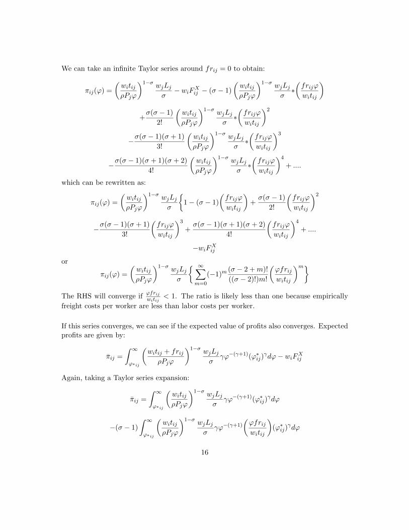
We can take an infinite Taylor series around frij = 0 to obtain:
πij(ϕ) =
(witijρPjϕ
)1−σ wjLjσ− wiFXij − (σ − 1)
(witijρPjϕ
)1−σ wjLjσ∗(frijϕ
witij
)
+σ(σ − 1)
2!
(witijρPjϕ
)1−σ wjLjσ∗(frijϕ
witij
)2
−σ(σ − 1)(σ + 1)
3!
(witijρPjϕ
)1−σ wjLjσ∗(frijϕ
witij
)3
−σ(σ − 1)(σ + 1)(σ + 2)
4!
(witijρPjϕ
)1−σ wjLjσ∗(frijϕ
witij
)4
+ ....
which can be rewritten as:
πij(ϕ) =
(witijρPjϕ
)1−σ wjLjσ
1− (σ − 1)
(frijϕ
witij
)+σ(σ − 1)
2!
(frijϕ
witij
)2
−σ(σ − 1)(σ + 1)
3!
(frijϕ
witij
)3
+σ(σ − 1)(σ + 1)(σ + 2)
4!
(frijϕ
witij
)4
+ ....
−wiFXijor
πij(ϕ) =
(witijρPjϕ
)1−σ wjLjσ
∞∑m=0
(−1)m(σ − 2 +m)!
((σ − 2)!)m!
(ϕfrijwitij
)mThe RHS will converge if
ϕfrijwitij
< 1. The ratio is likely less than one because empirically
freight costs per worker are less than labor costs per worker.
If this series converges, we can see if the expected value of profits also converges. Expectedprofits are given by:
πij =
ˆ ∞ϕ∗ij
(witij + frij
ρPjϕ
)1−σ wjLjσ
γϕ−(γ+1)(ϕ∗ij)γdϕ− wiFXij
Again, taking a Taylor series expansion:
πij =
ˆ ∞ϕ∗ij
(witijρPjϕ
)1−σ wjLjσ
γϕ−(γ+1)(ϕ∗ij)γdϕ
−(σ − 1)
ˆ ∞ϕ∗ij
(witijρPjϕ
)1−σ wjLjσ
γϕ−(γ+1)
(ϕfrijwitij
)(ϕ∗ij)
γdϕ
16
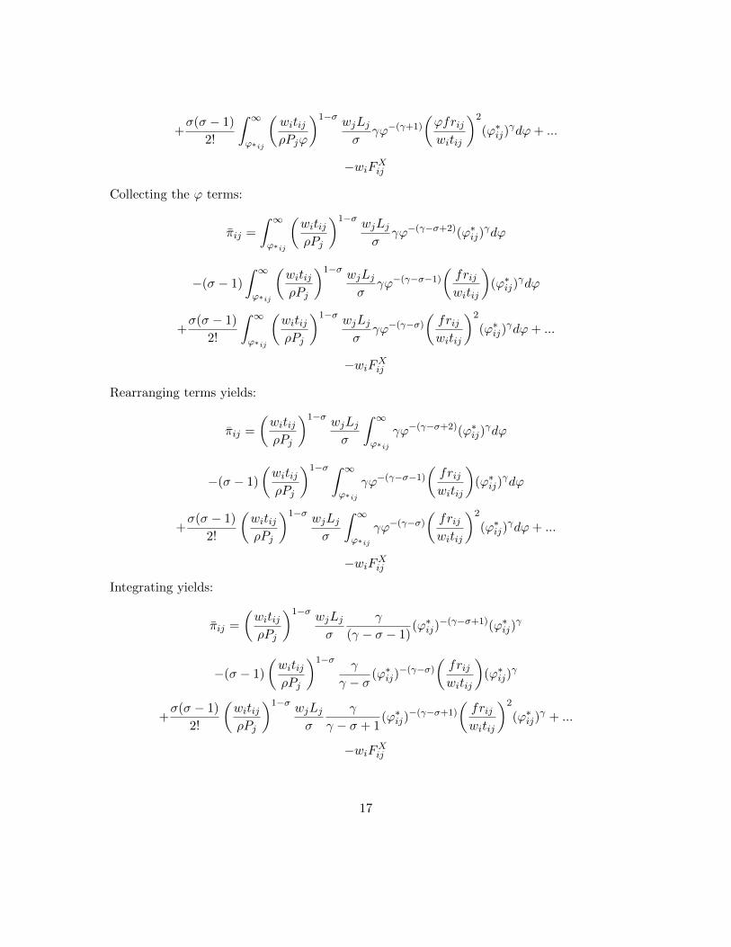
+σ(σ − 1)
2!
ˆ ∞ϕ∗ij
(witijρPjϕ
)1−σ wjLjσ
γϕ−(γ+1)
(ϕfrijwitij
)2
(ϕ∗ij)γdϕ+ ...
−wiFXij
Collecting the ϕ terms:
πij =
ˆ ∞ϕ∗ij
(witijρPj
)1−σ wjLjσ
γϕ−(γ−σ+2)(ϕ∗ij)γdϕ
−(σ − 1)
ˆ ∞ϕ∗ij
(witijρPj
)1−σ wjLjσ
γϕ−(γ−σ−1)
(frijwitij
)(ϕ∗ij)
γdϕ
+σ(σ − 1)
2!
ˆ ∞ϕ∗ij
(witijρPj
)1−σ wjLjσ
γϕ−(γ−σ)
(frijwitij
)2
(ϕ∗ij)γdϕ+ ...
−wiFXij
Rearranging terms yields:
πij =
(witijρPj
)1−σ wjLjσ
ˆ ∞ϕ∗ij
γϕ−(γ−σ+2)(ϕ∗ij)γdϕ
−(σ − 1)
(witijρPj
)1−σ ˆ ∞ϕ∗ij
γϕ−(γ−σ−1)
(frijwitij
)(ϕ∗ij)
γdϕ
+σ(σ − 1)
2!
(witijρPj
)1−σ wjLjσ
ˆ ∞ϕ∗ij
γϕ−(γ−σ)
(frijwitij
)2
(ϕ∗ij)γdϕ+ ...
−wiFXijIntegrating yields:
πij =
(witijρPj
)1−σ wjLjσ
γ
(γ − σ − 1)(ϕ∗ij)
−(γ−σ+1)(ϕ∗ij)γ
−(σ − 1)
(witijρPj
)1−σ γ
γ − σ(ϕ∗ij)
−(γ−σ)
(frijwitij
)(ϕ∗ij)
γ
+σ(σ − 1)
2!
(witijρPj
)1−σ wjLjσ
γ
γ − σ + 1(ϕ∗ij)
−(γ−σ+1)
(frijwitij
)2
(ϕ∗ij)γ + ...
−wiFXij
17
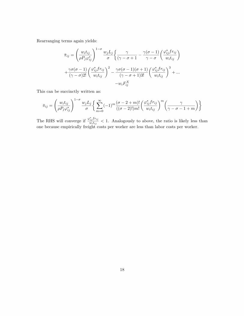
Rearranging terms again yields:
πij =
(witijρPjϕ∗ij
)1−σwjLjσ
γ
(γ − σ + 1− γ(σ − 1)
γ − σ
(ϕ∗ijfrij
witij
)
+γσ(σ − 1)
(γ − σ)2!
(ϕ∗ijfrij
witij
)2
− γσ(σ − 1)(σ + 1)
(γ − σ + 1)3!
(ϕ∗ijfrij
witij
)3
+ ...
−wiFXijThis can be succinctly written as:
πij =
(witijρPjϕ∗ij
)1−σwjLjσ
∞∑m=0
(−1)m(σ − 2 +m)!
((σ − 2)!)m!
(ϕ∗ijfrij
witij
)m( γ
γ − σ − 1 +m
)
The RHS will converge ifϕ∗ijfrijwitij
< 1. Analogously to above, the ratio is likely less than
one because empirically freight costs per worker are less than labor costs per worker.
18
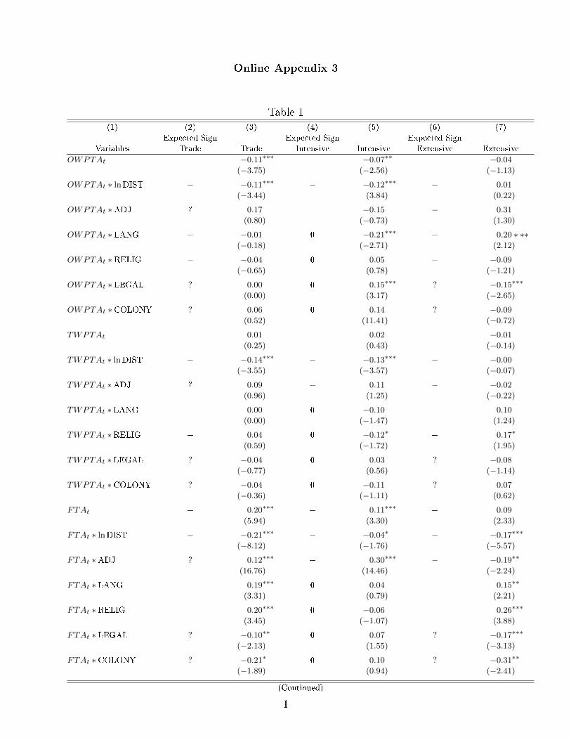
Online Appendix 3
Table 1
(1) (2) (3) (4) (5) (6) (7)
Expected Sign Expected Sign Expected Sign
Variables Trade Trade Intensive Intensive Extensive Extensive
OWPTAt + −0.11∗∗∗ + −0.07∗∗ + −0.04
(−3.75) (−2.56) (−1.13)
OWPTAt ∗ lnDIST − −0.11∗∗∗ − −0.12∗∗∗ − 0.01
(−3.44) (3.84) (0.22)
OWPTAt ∗ADJ ? 0.17 + −0.15 − 0.31
(0.80) (−0.73) (1.30)
OWPTAt ∗ LANG + −0.01 0 −0.21∗∗∗ + 0.20 ∗ ∗∗(−0.18) (−2.71) (2.12)
OWPTAt ∗ RELIG + −0.04 0 0.05 + −0.09
(−0.65) (0.78) (−1.21)
OWPTAt ∗ LEGAL ? 0.00 0 0.15∗∗∗ ? −0.15∗∗∗
(0.00) (3.17) (−2.65)
OWPTAt ∗ COLONY ? 0.06 0 0.14 ? −0.09
(0.52) (11.41) (−0.72)
TWPTAt + 0.01 + 0.02 + −0.01
(0.25) (0.43) (−0.14)
TWPTAt ∗ lnDIST − −0.14∗∗∗ − −0.13∗∗∗ − −0.00
(−3.55) (−3.57) (−0.07)
TWPTAt ∗ADJ ? 0.09 + 0.11 − −0.02
(0.96) (1.25) (−0.22)
TWPTAt ∗ LANG + 0.00 0 −0.10 + 0.10
(0.00) (−1.47) (1.24)
TWPTAt ∗ RELIG + 0.04 0 −0.12∗ + 0.17∗
(0.59) (−1.72) (1.95)
TWPTAt ∗ LEGAL ? −0.04 0 0.03 ? −0.08
(−0.77) (0.56) (−1.14)
TWPTAt ∗ COLONY ? −0.04 0 −0.11 ? 0.07
(−0.36) (−1.11) (0.62)
FTAt + 0.20∗∗∗ + 0.11∗∗∗ + 0.09
(5.94) (3.30) (2.33)
FTAt ∗ lnDIST − −0.21∗∗∗ − −0.04∗ − −0.17∗∗∗
(−8.12) (−1.76) (−5.57)
FTAt ∗ADJ ? 0.12∗∗∗ + 0.30∗∗∗ − −0.19∗∗
(16.76) (14.46) (−2.24)
FTAt ∗ LANG + 0.19∗∗∗ 0 0.04 + 0.15∗∗
(3.31) (0.79) (2.21)
FTAt ∗ RELIG + 0.20∗∗∗ 0 −0.06 + 0.26∗∗∗
(3.45) (−1.07) (3.88)
FTAt ∗ LEGAL ? −0.10∗∗ 0 0.07 ? −0.17∗∗∗
(−2.13) (1.55) (−3.13)
FTAt ∗ COLONY ? −0.21∗ 0 0.10 ? −0.31∗∗
(−1.89) (0.94) (−2.41)
(Continued)
1
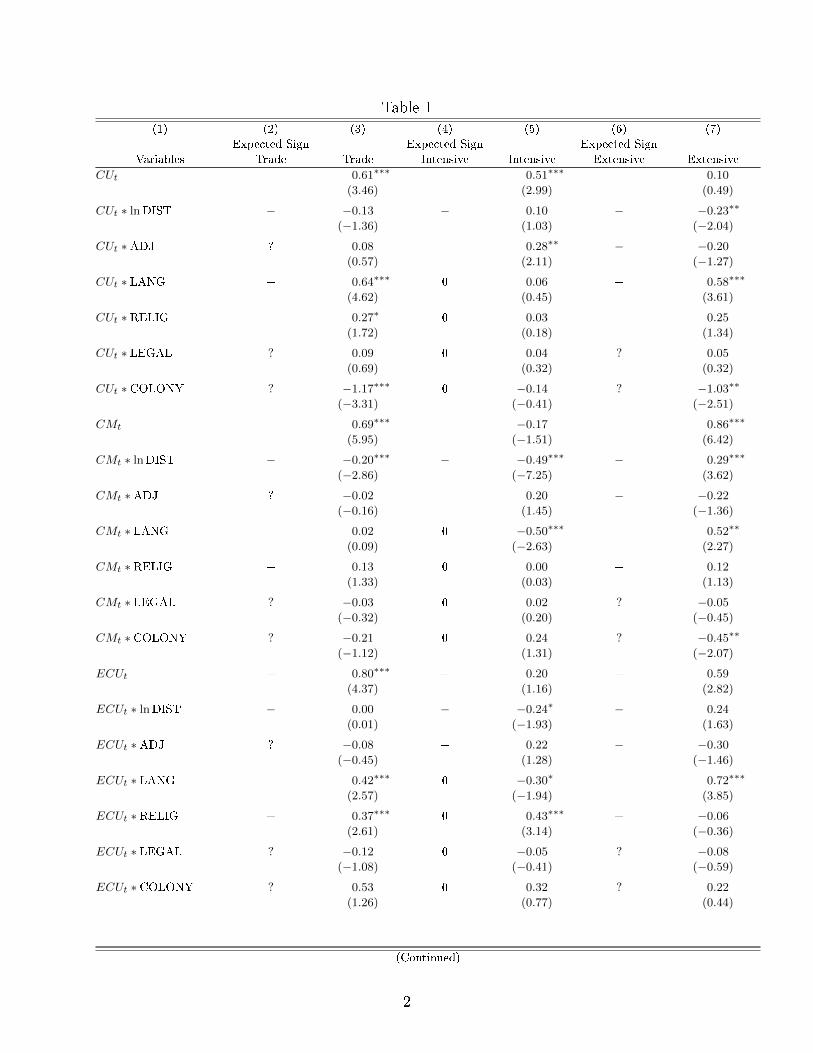
Table 1
(1) (2) (3) (4) (5) (6) (7)
Expected Sign Expected Sign Expected Sign
Variables Trade Trade Intensive Intensive Extensive Extensive
CUt + 0.61∗∗∗ + 0.51∗∗∗ + 0.10
(3.46) (2.99) (0.49)
CUt ∗ lnDIST − −0.13 − 0.10 − −0.23∗∗
(−1.36) (1.03) (−2.04)
CUt ∗ADJ ? 0.08 + 0.28∗∗ − −0.20
(0.57) (2.11) (−1.27)
CUt ∗ LANG + 0.64∗∗∗ 0 0.06 + 0.58∗∗∗
(4.62) (0.45) (3.61)
CUt ∗ RELIG + 0.27∗ 0 0.03 + 0.25
(1.72) (0.18) (1.34)
CUt ∗ LEGAL ? 0.09 0 0.04 ? 0.05
(0.69) (0.32) (0.32)
CUt ∗ COLONY ? −1.17∗∗∗ 0 −0.14 ? −1.03∗∗
(−3.31) (−0.41) (−2.51)
CMt + 0.69∗∗∗ + −0.17 + 0.86∗∗∗
(5.95) (−1.51) (6.42)
CMt ∗ lnDIST − −0.20∗∗∗ − −0.49∗∗∗ − 0.29∗∗∗
(−2.86) (−7.25) (3.62)
CMt ∗ADJ ? −0.02 + 0.20 − −0.22
(−0.16) (1.45) (−1.36)
CMt ∗ LANG + 0.02 0 −0.50∗∗∗ + 0.52∗∗
(0.09) (−2.63) (2.27)
CMt ∗ RELIG + 0.13 0 0.00 + 0.12
(1.33) (0.03) (1.13)
CMt ∗ LEGAL ? −0.03 0 0.02 ? −0.05
(−0.32) (0.20) (−0.45)
CMt ∗ COLONY ? −0.21 0 0.24 ? −0.45∗∗
(−1.12) (1.31) (−2.07)
ECUt + 0.80∗∗∗ + 0.20 + 0.59
(4.37) (1.16) (2.82)
ECUt ∗ lnDIST − 0.00 − −0.24∗ − 0.24
(0.01) (−1.93) (1.63)
ECUt ∗ADJ ? −0.08 + 0.22 − −0.30
(−0.45) (1.28) (−1.46)
ECUt ∗ LANG + 0.42∗∗∗ 0 −0.30∗ + 0.72∗∗∗
(2.57) (−1.94) (3.85)
ECUt ∗ RELIG + 0.37∗∗∗ 0 0.43∗∗∗ + −0.06
(2.61) (3.14) (−0.36)
ECUt ∗ LEGAL ? −0.12 0 −0.05 ? −0.08
(−1.08) (−0.41) (−0.59)
ECUt ∗ COLONY ? 0.53 0 0.32 ? 0.22
(1.26) (0.77) (0.44)
(Continued)
2
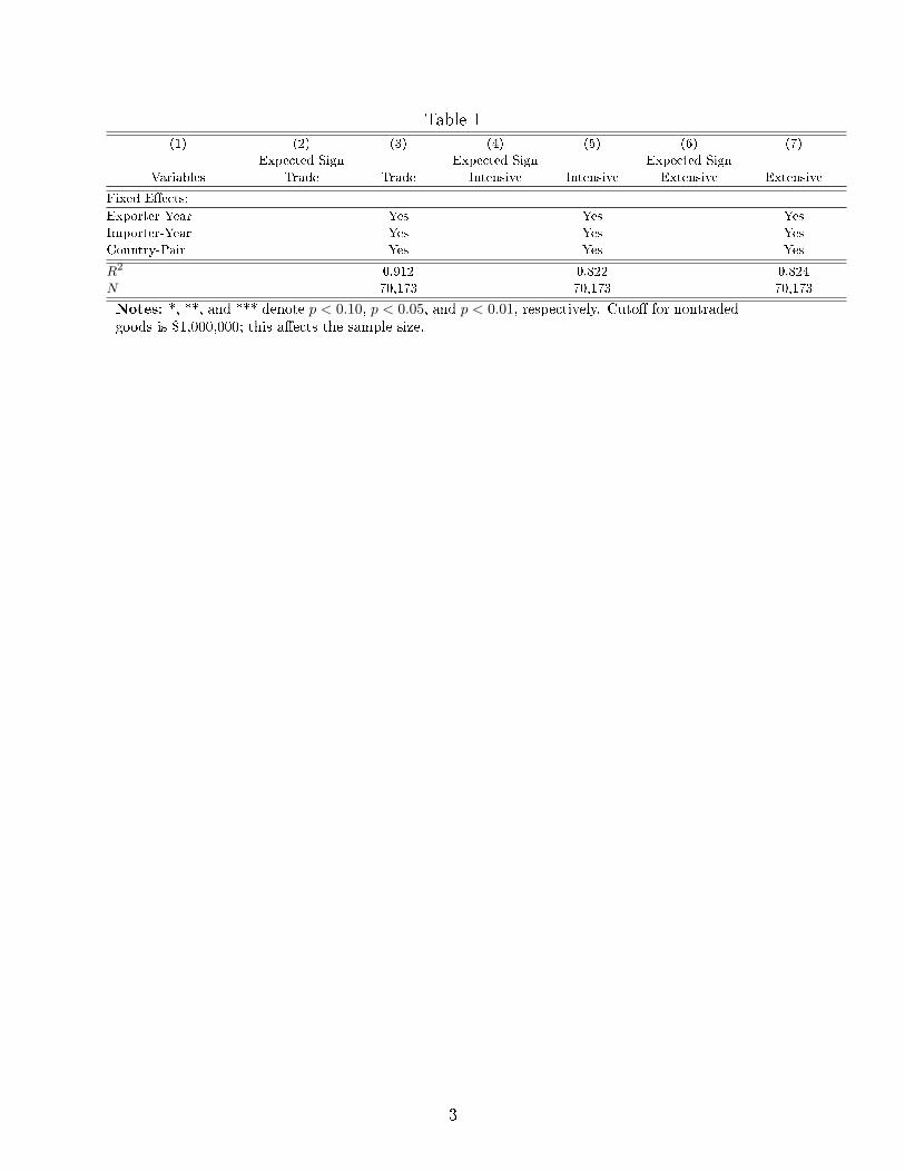
Table 1
(1) (2) (3) (4) (5) (6) (7)
Expected Sign Expected Sign Expected Sign
Variables Trade Trade Intensive Intensive Extensive Extensive
Fixed Eects:
Exporter-Year Yes Yes Yes
Importer-Year Yes Yes Yes
Country-Pair Yes Yes Yes
R2 0.912 0.822 0.824
N 70,173 70,173 70,173
Notes: *, **, and *** denote p < 0.10, p < 0.05, and p < 0.01, respectively. Cuto for nontradedgoods is $1,000,000; this aects the sample size.
3
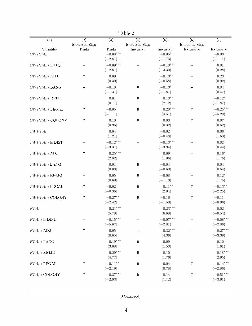
Table 2
(1) (2) (3) (4) (5) (6) (7)
Expected Sign Expected Sign Expected Sign
Variables Trade Trade Intensive Intensive Extensive Extensive
OWPTAt + −0.08∗∗∗ + −0.05∗ + −0.03
(−2.81) (−1.73) (−1.11)
OWPTAt ∗ lnDIST − −0.09∗∗∗ − −0.10∗∗∗ − 0.01
(−2.81) (−3.30) (0.28)
OWPTAt ∗ADJ ? 0.09 + −0.13∗∗ − 0.23
(0.39) (−0.58) (0.92)
OWPTAt ∗ LANG + −0.10 0 −0.13∗ + 0.04
(−1.31) (−1.87) (0.47)
OWPTAt ∗ RELIG + 0.01 0 0.13∗∗ + −0.12∗
(0.11) (2.12) (−1.87)
OWPTAt ∗ LEGAL ? −0.05 0 0.20∗∗∗ ? −0.25∗∗∗
(−1.11) (4.51) (−5.29)
OWPTAt ∗ COLONY ? 0.10 0 0.03 ? 0.07
(0.96) (0.32) (0.62)
TWPTAt + 0.04 + −0.02 + 0.06
(1.21) (−0.48) (1.63)
TWPTAt ∗ lnDIST − −0.12∗∗∗ − −0.13∗∗∗ − 0.02
(−3.37) (−3.94) (0.44)
TWPTAt ∗ADJ ? 0.25∗∗∗ + 0.09 − 0.16∗
(2.82) (1.06) (1.76)
TWPTAt ∗ LANG + 0.01 0 −0.04 + 0.04
(0.08) (−0.60) (0.64)
TWPTAt ∗ RELIG + 0.05 0 −0.08 + 0.12∗
(0.69) (−1.13) (1.75)
TWPTAt ∗ LEGAL ? −0.02 0 0.11∗∗ ? −0.13∗∗
(−0.36) (2.04) (−2.25)
TWPTAt ∗ COLONY ? −0.27∗∗ 0 −0.16 ? −0.11
(−2.42) (−1.50) (−0.96)
FTAt + 0.21∗∗∗ + 0.23∗∗∗ + −0.02
(5.78) (6.68) (−0.54)
FTAt ∗ lnDIST − −0.15∗∗∗ − −0.07∗∗∗ − −0.08∗∗∗
(−5.67) (−2.81) (−2.86)
FTAt ∗ADJ ? 0.05 + 0.32∗∗∗ − −0.27∗∗∗
(0.65) (4.36) (−3.39)
FTAt ∗ LANG + 0.19∗∗∗ 0 0.09 + 0.10
(3.08) (1.53) (1.61)
FTAt ∗ RELIG + 0.29∗∗∗ 0 0.10 + 0.18∗∗∗
(4.77) (1.76) (2.95)
FTAt ∗ LEGAL ? −0.11∗∗ 0 0.04 ? −0.14∗∗∗
(−2.19) (0.78) (−2.86)
FTAt ∗ COLONY ? −0.37∗∗∗ 0 0.14 ? −0.51∗∗∗
(−2.93) (1.12) (−3.91)
(Continued)
4
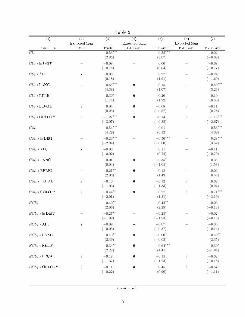
Table 2
(1) (2) (3) (4) (5) (6) (7)
Expected Sign Expected Sign Expected Sign
Variables Trade Trade Intensive Intensive Extensive Extensive
CUt + 0.53∗∗∗ + 0.55∗∗∗ + −0.02
(2.85) (3.07) (−0.09)
CUt ∗ lnDIST − −0.08 − 0.00 − −0.08
(−0.76) (0.04) (−0.77)
CUt ∗ADJ ? 0.03 + 0.27∗ − −0.24
(0.18) (1.91) (−1.60)
CUt ∗ LANG + 0.65∗∗∗ 0 0.15 + 0.50∗∗∗
(4.38) (1.07) (3.26)
CUt ∗ RELIG + 0.30∗ 0 0.20 + 0.10
(1.74) (1.22) (0.56)
CUt ∗ LEGAL ? 0.04 0 −0.08 ? −0.11
(0.25) (−0.57) (0.78)
CUt ∗ COLONY ? −1.27∗∗∗ 0 −0.14 ? −1.13∗∗∗
(−3.07) (−0.35) (−2.67)
CMt + 0.54∗∗∗ + 0.01 + 0.53∗∗∗
(4.29) (0.12) (4.09)
CMt ∗ lnDIST − −0.23∗∗∗ − −0.50∗∗∗ − 0.28∗∗∗
(−2.94) (−6.80) (3.52)
CMt ∗ADJ ? −0.03 + 0.11 − −0.11
(−0.02) (0.72) (−0.70)
CMt ∗ LANG + 0.01 0 −0.35∗ + 0.35
(0.04) (−1.65) (1.58)
CMt ∗ RELIG + 0.21∗∗ 0 0.15 + 0.06
(2.03) (1.49) (0.58)
CMt ∗ LEGAL ? −0.10 0 −0.12 ? 0.02
(−1.03) (−1.33) (0.24)
CMt ∗ COLONY ? −0.44∗∗ 0 0.27 ? −0.71∗∗∗
(−2.01) (1.31) (−3.19)
ECUt + 0.40∗∗ + 0.42∗∗ + −0.03
(2.06) (2.29) (−0.13)
ECUt ∗ lnDIST − −0.27∗∗ − −0.25∗ − −0.02
(−1.99) (−1.93) (−0.15)
ECUt ∗ADJ ? −0.09 + −0.07 − −0.03
(−0.05) (−0.37) (−0.14)
ECUt ∗ LANG + 0.40∗∗ 0 −0.00∗ + 0.40∗∗
(2.39) (−0.03) (2.35)
ECUt ∗ RELIG + 0.34∗∗ 0 0.64∗∗∗ + −0.30∗
(2.22) (4.41) (−1.94)
ECUt ∗ LEGAL ? −0.18 0 −0.15 ? −0.02
(−1.37) (−1.23) (−0.18)
ECUt ∗ COLONY ? −0.11 0 0.45 ? −0.57
(−0.22) (0.96) (−1.11)
(Continued)
5
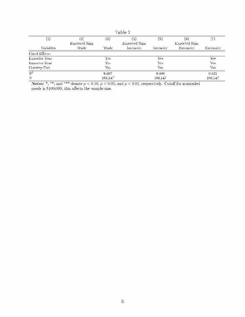
Table 2
(1) (2) (3) (4) (5) (6) (7)
Expected Sign Expected Sign Expected Sign
Variables Trade Trade Intensive Intensive Extensive Extensive
Fixed Eects:
Exporter-Year Yes Yes Yes
Importer-Year Yes Yes Yes
Country-Pair Yes Yes Yes
R2 0.897 0.800 0.821
N 103,147 103,147 103,147
Notes: *, **, and *** denote p < 0.10, p < 0.05, and p < 0.01, respectively. Cuto for nontradedgoods is $100,000; this aects the sample size.
6
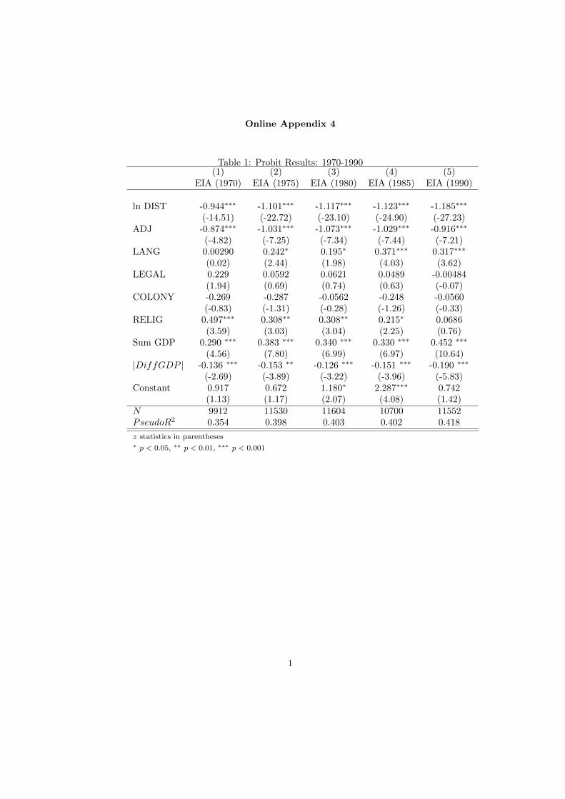
Online Appendix 4
Table 1: Probit Results: 1970-1990(1) (2) (3) (4) (5)
EIA (1970) EIA (1975) EIA (1980) EIA (1985) EIA (1990)
ln DIST -0.944∗∗∗ -1.101∗∗∗ -1.117∗∗∗ -1.123∗∗∗ -1.185∗∗∗
(-14.51) (-22.72) (-23.10) (-24.90) (-27.23)ADJ -0.874∗∗∗ -1.031∗∗∗ -1.073∗∗∗ -1.029∗∗∗ -0.916∗∗∗
(-4.82) (-7.25) (-7.34) (-7.44) (-7.21)LANG 0.00290 0.242∗ 0.195∗ 0.371∗∗∗ 0.317∗∗∗
(0.02) (2.44) (1.98) (4.03) (3.62)LEGAL 0.229 0.0592 0.0621 0.0489 -0.00484
(1.94) (0.69) (0.74) (0.63) (-0.07)COLONY -0.269 -0.287 -0.0562 -0.248 -0.0560
(-0.83) (-1.31) (-0.28) (-1.26) (-0.33)RELIG 0.497∗∗∗ 0.308∗∗ 0.308∗∗ 0.215∗ 0.0686
(3.59) (3.03) (3.04) (2.25) (0.76)Sum GDP 0.290 ∗∗∗ 0.383 ∗∗∗ 0.340 ∗∗∗ 0.330 ∗∗∗ 0.452 ∗∗∗
(4.56) (7.80) (6.99) (6.97) (10.64)|DiffGDP | -0.136 ∗∗∗ -0.153 ∗∗ -0.126 ∗∗∗ -0.151 ∗∗∗ -0.190 ∗∗∗
(-2.69) (-3.89) (-3.22) (-3.96) (-5.83)Constant 0.917 0.672 1.180∗ 2.287∗∗∗ 0.742
(1.13) (1.17) (2.07) (4.08) (1.42)N 9912 11530 11604 10700 11552PseudoR2 0.354 0.398 0.403 0.402 0.418
z statistics in parentheses∗ p < 0.05, ∗∗ p < 0.01, ∗∗∗ p < 0.001
1
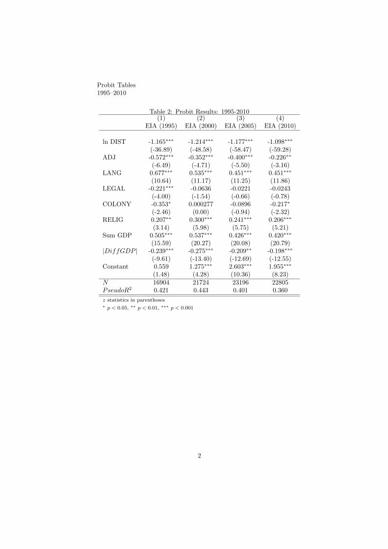
Probit Tables1995–2010
Table 2: Probit Results: 1995-2010(1) (2) (3) (4)
EIA (1995) EIA (2000) EIA (2005) EIA (2010)
ln DIST -1.165∗∗∗ -1.214∗∗∗ -1.177∗∗∗ -1.098∗∗∗
(-36.89) (-48.58) (-58.47) (-59.28)ADJ -0.572∗∗∗ -0.352∗∗∗ -0.400∗∗∗ -0.226∗∗
(-6.49) (-4.71) (-5.50) (-3.16)LANG 0.677∗∗∗ 0.535∗∗∗ 0.451∗∗∗ 0.451∗∗∗
(10.64) (11.17) (11.25) (11.86)LEGAL -0.221∗∗∗ -0.0636 -0.0221 -0.0243
(-4.00) (-1.54) (-0.66) (-0.78)COLONY -0.353∗ 0.000277 -0.0896 -0.217∗
(-2.46) (0.00) (-0.94) (-2.32)RELIG 0.207∗∗ 0.300∗∗∗ 0.241∗∗∗ 0.206∗∗∗
(3.14) (5.98) (5.75) (5.21)Sum GDP 0.505∗∗∗ 0.537∗∗∗ 0.426∗∗∗ 0.420∗∗∗
(15.59) (20.27) (20.08) (20.79)|DiffGDP | -0.239∗∗∗ -0.275∗∗∗ -0.209∗∗ -0.198∗∗∗
(-9.61) (-13.40) (-12.69) (-12.55)Constant 0.559 1.275∗∗∗ 2.603∗∗∗ 1.955∗∗∗
(1.48) (4.28) (10.36) (8.23)N 16904 21724 23196 22805PseudoR2 0.421 0.443 0.401 0.360
z statistics in parentheses∗ p < 0.05, ∗∗ p < 0.01, ∗∗∗ p < 0.001
2


![Communication Skills [CMS] - Vidyalankardiploma.vidyalankar.org/wp-content/uploads/mech.pdf · acceleration and uniform retardation, equations of motion for motion under gravity](https://img.pdfslide.us/doc/110x75/5aa1f9327f8b9a1f6d8c9cbf/communication-skills-cms-and-uniform-retardation-equations-of-motion-for-motion.jpg)