Notes on “Gravitation” (Misner et al., 1973)

Robert B. Scott,1,2∗

1Institute for Geophysics, Jackson School of Geosciences, The University of Texas at Austin,

Austin, Texas, USA2Department of Physics, University of Brest,

Brest, France

∗To whom correspondence should be addressed; E-mail: rscott@ig.utexas.edu.

January 27, 2012

2

Part I

Spacetime physics

3

Chapter 1

Geometrodynamics in brief

1.5 Time

Time is defined so that motion looks simple. So free particles move in straightlines at constant speeds. But how do we decide what a straight line is?

1.6 Curvature

Typo: Eq. (1.11), the 3rd α should be a β so that it reads:

D2xα

Dτ 2− e

mFα

β

dxβ

dτ= 0

This corresponds to (Hobson et al., 2009, Eq. (6.13)).

1.7 Exercises

Exercise 1.1: Curvature of a cylinderShow that the Gaussian curvature R of the surface of a cylinder is zero by

showing that geodesics on that surface (unroll!) suffer no geodesic deviation.Give an independent argument for the same conclusion by employing the

5

6

formula R = 1/ρ1ρ2 where ρ1 and ρ2 are the principal radii of curvature at thepoint in question with respect to the enveloping Euclidean three-dimensionalspace.

Solution:The Gaussian curvature R, and the principal radii of curvature were not

precisely defined in the text, making this question a bit intimidating. Theyare actually quite simple, and explained clearly by Faber (1983, p. 17). How-ever, we can make progress with the given “equation of geodesic deviation”,Eqn. (1.6),

d2ξ

ds2+Rξ = 0

where ξ is the “geodesic deviation”, the distance between geodesics, c.f.Fig. 1.10. Unrolling the cylinder doesn’t change the distances between geodesics,and helps reveal instantly that parallel geodesics have constant separation.From Eqn. (1.6), this can only be true if R = 0.

The independent argument requires knowing what the “principal radii ofcurvature” are. One might guess that these are the extremma of radii ofcurvature of the curves that mark the intersect of the surface with orthogo-nal planes. If one orients the plans such that ρ1 is minimum, the radius ofthe cylinder, then the other is maximum, i.e. ρ2 =∞. Indeed, this assump-tion is confirmed http://en.wikipedia.org/wiki/Radius_of_curvature_

(applications). Better yet, read (Faber, 1983, § 1.2). In short, a cyclinderhas no curvature along its length. An immediate consequence appears to bethat R is zero and parallel geodesics have constant separation.

Exercise 1.2: Spring tide vs. neap tide Evaluate (1) in conventionalunits and (2) in geometrized units the magnitude of the Newtonian tide-producing acceleration Rk

0j0(k, j = 1, 2, 3) generated at the Earth by (1) themoon (mconv = 7.35× 1025[g], r = 3.84× 1010[cm]) and (2) the sun. By whatfactor do you expect spring tides to exceed neap tides? [I’ve changed indices(m,n) to (k, j) because m could be confused with the mass.]

Solution:

7

Eqn. (1.5) gives the acceleration of a test particle relative to a fiducialparticle due to tide producing forces. The test particles can be viewed asmoving along geodesics in a Lorentzian frame of reference. The equation ofgeodesic deviations is given by Eqn. (1.13). Equating these equations givesthe components of the terms of Riemann curvature tensor:

Rk0j0 =

Gmconv

r3= 8.66× 10−14 sec−2

Note that despite being called “acceleration” by MTW, they have units offrequency squared.

Rk0j0 =

Gmconv

c2r3δk,j, k ∈ {1, 2} =

m

r3= 0.00545[cm] 1/r3 = 9.63×10−35cm−2

For the radial component, k = j = 3:

Rk0j0 = −2

Gmconv

r3= 17.32× 10−14cm sec−2 = −1.93× 10−34cm−2

Repeating the exercise for the Sun, one finds numbers almost 1/2 as big.For the radial component:

Rk0j0 =

Gmconv

r3= 3.96× 10−14sec−2

As a physical oceanographer of course I quite like this question! ButI find it’s a bit confusing too since there are so many aspects of tides tocompare: tidal velocities, tidal ellipses, etc. Probably most people think ofhow far up and down the shore the water goes, so I would guess that hereMTW are asking about tidal amplitude of sea surface height. Predictingthe oceanic tides requires complex, global, numerical models (?) because thetides are not in hydrostatic balance. It turns out that in most places the tidesproduced by the Sun, S1 in oceanography lingo, are about 1/2 the amplitudeof those produced by the Moon, the M2 tides. During spring tide, the solarand lunar tides combine, while during neap tide there is partial cancellation.The spring tide should be 3 times larger than neap tide.

It seems quite naive to me to assume that the tidal vertical displacementamplitude should be proportional to the forcing. The frequency of the M2tides is about twice that of the S1 tides and this must be a factor as well.

8

Exercise 1.3: Kepler encapsulated A small satellite has a circular fre-quency ω[cm−1] in an orbit or radius r about a central object of mass m[cm].From the known value of ω show that it’s not possible to determine neitherr nor m individually, but only the effective “Kepler density” of the object asaveraged over a sphere of the same radius as the orbit. Give the formula forω2 in terms of this Kepler density.

Solution:Balance the centripetal acceleration with the Newtonian gravitational

acceleration,

ω2(cm sec−2) r =Gmconv

r2

Or

ω2(rad cm−1) r =Gmconv

c2r2=m

r2

So given only ω one can determine the ratio of the mass to orbit radius cubed,but not m nor r individually:

ω2(rad cm−2) =m

r3.

The Kepler density is apparently ρK ≡ 3m/(4πr3), so

ω2 =4π

3ρK .

See also Figure 1.12.

Part II

Physics in flat spacetime

9

Chapter 2

Foundations of special relativity

Box 2.2 Horrible choice of notation. The four-velocity and four-momentumvectors are denoted in bold face sans-serif font. The spatial parts of thesefour-vectors, which in general of course are not just the corresponding three-vectors, are denoted also by bold fact but a slightly different font! If youlook really closely you can make out the difference, but only if you’re lookingfor it!! And we’re not even warned of this until a few pages later. So forinstance, in the First Solution, second line of the equation,

p2 = −(mu0)2 +m2u2

that’s not a typo! The u2 is just the spatial part of the four-velocity squared.

2.5 Differential Forms

First equation (un-numbered, see bottom p. 53), defining the four momen-tum. The mass here is the rest mass, not the relativistic mass.

Exercise 2.1: Show that equation (2.14) is in accord with the quan-tum mechanical properties of a de Broglie wave

ψ = exp(iφ) = exp[i(k · x− ωt)]

11

12

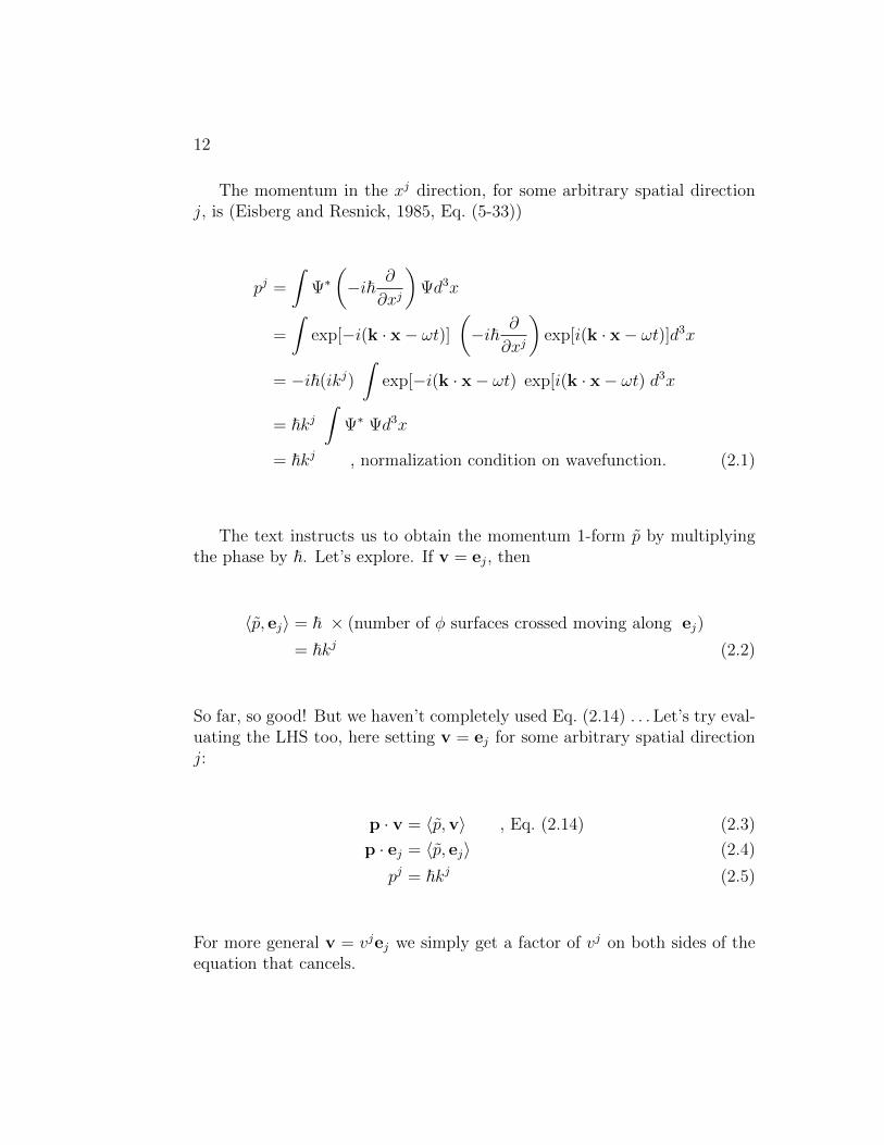
The momentum in the xj direction, for some arbitrary spatial directionj, is (Eisberg and Resnick, 1985, Eq. (5-33))

pj =

∫Ψ∗(−i~ ∂

∂xj

)Ψd3x

=

∫exp[−i(k · x− ωt)]

(−i~ ∂

∂xj

)exp[i(k · x− ωt)]d3x

= −i~(ikj)

∫exp[−i(k · x− ωt) exp[i(k · x− ωt) d3x

= ~kj∫

Ψ∗ Ψd3x

= ~kj , normalization condition on wavefunction. (2.1)

The text instructs us to obtain the momentum 1-form p by multiplyingthe phase by ~. Let’s explore. If v = ej, then

〈p, ej〉 = ~ × (number of φ surfaces crossed moving along ej)

= ~kj (2.2)

So far, so good! But we haven’t completely used Eq. (2.14) . . . Let’s try eval-uating the LHS too, here setting v = ej for some arbitrary spatial directionj:

p · v = 〈p,v〉 , Eq. (2.14) (2.3)

p · ej = 〈p, ej〉 (2.4)

pj = ~kj (2.5)

For more general v = vjej we simply get a factor of vj on both sides of theequation that cancels.

13

2.6 Gradients and directional derivatives

2.7 Coordinate representation of geometric

objects

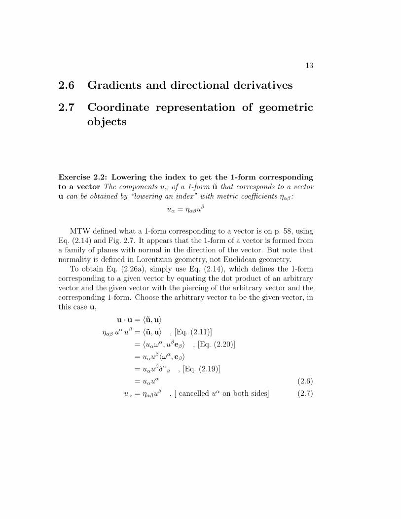
Exercise 2.2: Lowering the index to get the 1-form correspondingto a vector The components uα of a 1-form u that corresponds to a vectoru can be obtained by “lowering an index” with metric coefficients ηαβ:

uα = ηαβuβ

MTW defined what a 1-form corresponding to a vector is on p. 58, usingEq. (2.14) and Fig. 2.7. It appears that the 1-form of a vector is formed froma family of planes with normal in the direction of the vector. But note thatnormality is defined in Lorentzian geometry, not Euclidean geometry.

To obtain Eq. (2.26a), simply use Eq. (2.14), which defines the 1-formcorresponding to a given vector by equating the dot product of an arbitraryvector and the given vector with the piercing of the arbitrary vector and thecorresponding 1-form. Choose the arbitrary vector to be the given vector, inthis case u,

u · u = 〈u,u〉ηαβ u

α uβ = 〈u,u〉 , [Eq. (2.11)]

= 〈uαωα, uβeβ〉 , [Eq. (2.20)]

= uαuβ〈ωα, eβ〉

= uαuβδαβ , [Eq. (2.19)]

= uαuα (2.6)

uα = ηαβuβ , [ cancelled uα on both sides] (2.7)

14

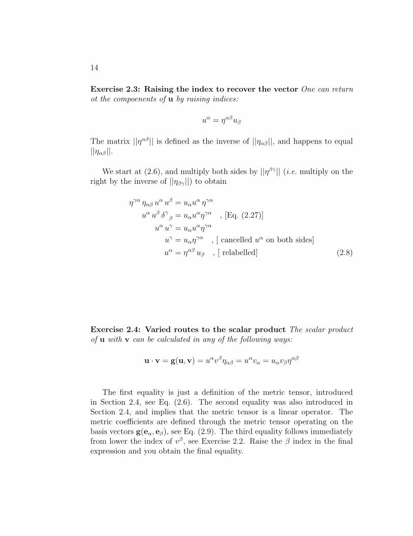
Exercise 2.3: Raising the index to recover the vector One can returnot the compoenents of u by raising indices:

uα = ηαβuβ

The matrix ||ηαβ|| is defined as the inverse of ||ηαβ||, and happens to equal||ηαβ||.

We start at (2.6), and multiply both sides by ||ηβγ|| (i.e. multiply on theright by the inverse of ||ηβγ||) to obtain

ηγα ηαβ uα uβ = uαu

α ηγα

uα uβ δγ β = uαuαηγα , [Eq. (2.27)]

uα uγ = uαuαηγα

uγ = uαηγα , [ cancelled uα on both sides]

uα = ηαβ uβ , [ relabelled] (2.8)

Exercise 2.4: Varied routes to the scalar product The scalar productof u with v can be calculated in any of the following ways:

u · v = g(u,v) = uαvβηαβ = uαvα = uαvβηαβ

The first equality is just a definition of the metric tensor, introducedin Section 2.4, see Eq. (2.6). The second equality was also introduced inSection 2.4, and implies that the metric tensor is a linear operator. Themetric coefficients are defined through the metric tensor operating on thebasis vectors g(eα, eβ), see Eq. (2.9). The third equality follows immediatelyfrom lower the index of vβ, see Exercise 2.2. Raise the β index in the finalexpression and you obtain the final equality.

15

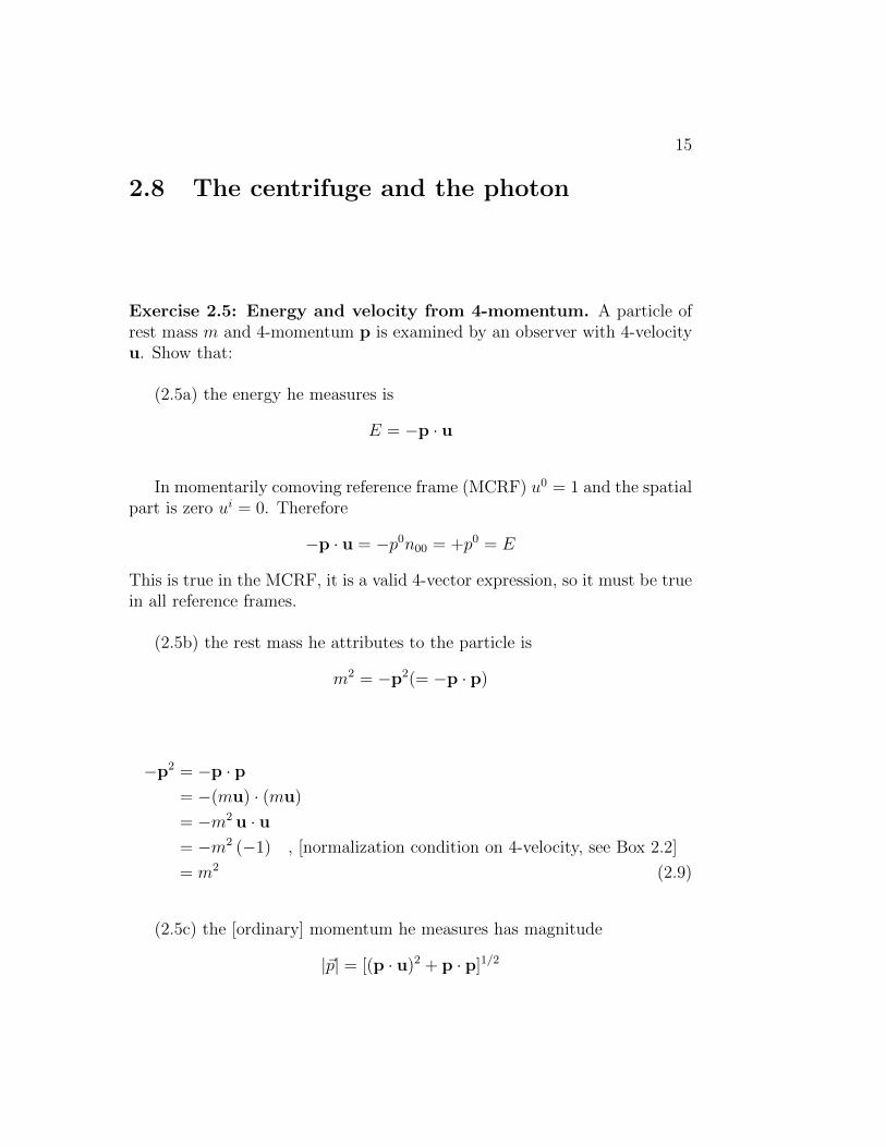
2.8 The centrifuge and the photon

Exercise 2.5: Energy and velocity from 4-momentum. A particle ofrest mass m and 4-momentum p is examined by an observer with 4-velocityu. Show that:

(2.5a) the energy he measures is

E = −p · u

In momentarily comoving reference frame (MCRF) u0 = 1 and the spatialpart is zero ui = 0. Therefore

−p · u = −p0n00 = +p0 = E

This is true in the MCRF, it is a valid 4-vector expression, so it must be truein all reference frames.

(2.5b) the rest mass he attributes to the particle is

m2 = −p2(= −p · p)

−p2 = −p · p= −(mu) · (mu)

= −m2 u · u= −m2 (−1) , [normalization condition on 4-velocity, see Box 2.2]

= m2 (2.9)

(2.5c) the [ordinary] momentum he measures has magnitude

|~p| = [(p · u)2 + p · p]1/2

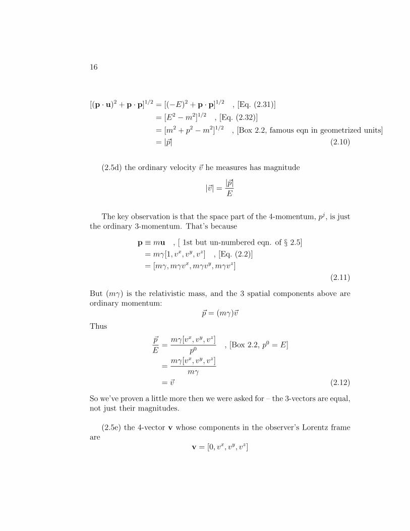
16

[(p · u)2 + p · p]1/2 = [(−E)2 + p · p]1/2 , [Eq. (2.31)]

= [E2 −m2]1/2 , [Eq. (2.32)]

= [m2 + p2 −m2]1/2 , [Box 2.2, famous eqn in geometrized units]

= |~p| (2.10)

(2.5d) the ordinary velocity ~v he measures has magnitude

|~v| = |~p|E

The key observation is that the space part of the 4-momentum, pj, is justthe ordinary 3-momentum. That’s because

p ≡ mu , [ 1st but un-numbered eqn. of § 2.5]

= mγ[1, vx, vy, vz] , [Eq. (2.2)]

= [mγ,mγvx,mγvy,mγvz]

(2.11)

But (mγ) is the relativistic mass, and the 3 spatial components above areordinary momentum:

~p = (mγ)~v

Thus

~p

E=mγ[vx, vy, vz]

p0, [Box 2.2, p0 = E]

=mγ[vx, vy, vz]

mγ

= ~v (2.12)

So we’ve proven a little more then we were asked for – the 3-vectors are equal,not just their magnitudes.

(2.5e) the 4-vector v whose components in the observer’s Lorentz frameare

v = [0, vx, vy, vz]

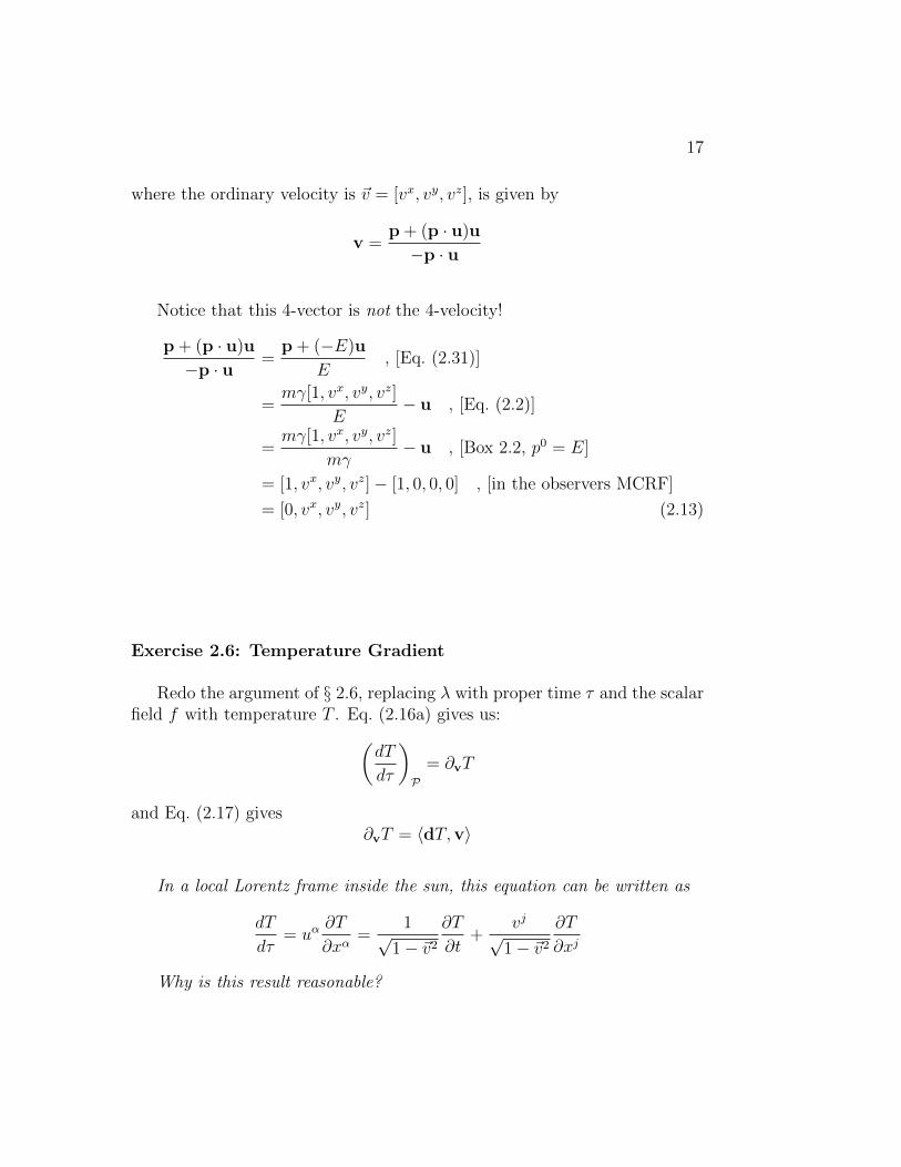
17

where the ordinary velocity is ~v = [vx, vy, vz], is given by

v =p + (p · u)u

−p · u

Notice that this 4-vector is not the 4-velocity!

p + (p · u)u

−p · u=

p + (−E)u

E, [Eq. (2.31)]

=mγ[1, vx, vy, vz]

E− u , [Eq. (2.2)]

=mγ[1, vx, vy, vz]

mγ− u , [Box 2.2, p0 = E]

= [1, vx, vy, vz]− [1, 0, 0, 0] , [in the observers MCRF]

= [0, vx, vy, vz] (2.13)

Exercise 2.6: Temperature Gradient

Redo the argument of § 2.6, replacing λ with proper time τ and the scalarfield f with temperature T . Eq. (2.16a) gives us:(

dT

dτ

)P

= ∂vT

and Eq. (2.17) gives∂vT = 〈dT,v〉

In a local Lorentz frame inside the sun, this equation can be written as

dT

dτ= uα

∂T

∂xα=

1√1− ~v2

∂T

∂t+

vj√1− ~v2

∂T

∂xj

Why is this result reasonable?

18

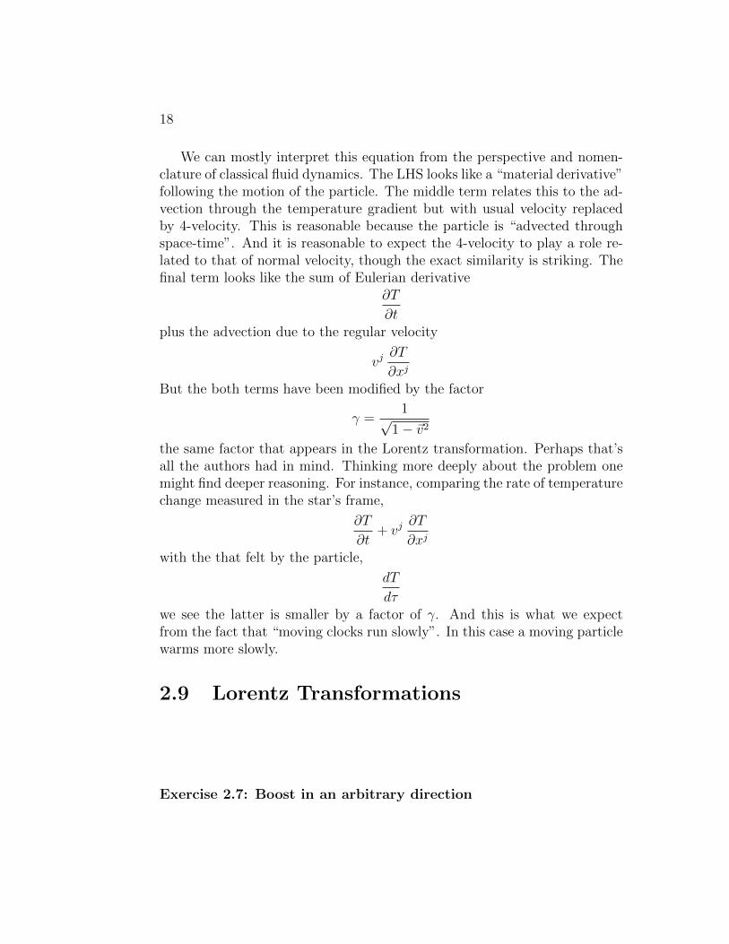
We can mostly interpret this equation from the perspective and nomen-clature of classical fluid dynamics. The LHS looks like a “material derivative”following the motion of the particle. The middle term relates this to the ad-vection through the temperature gradient but with usual velocity replacedby 4-velocity. This is reasonable because the particle is “advected throughspace-time”. And it is reasonable to expect the 4-velocity to play a role re-lated to that of normal velocity, though the exact similarity is striking. Thefinal term looks like the sum of Eulerian derivative

∂T

∂tplus the advection due to the regular velocity

vj∂T

∂xj

But the both terms have been modified by the factor

γ =1√

1− ~v2the same factor that appears in the Lorentz transformation. Perhaps that’sall the authors had in mind. Thinking more deeply about the problem onemight find deeper reasoning. For instance, comparing the rate of temperaturechange measured in the star’s frame,

∂T

∂t+ vj

∂T

∂xj

with the that felt by the particle,

dT

dτwe see the latter is smaller by a factor of γ. And this is what we expectfrom the fact that “moving clocks run slowly”. In this case a moving particlewarms more slowly.

2.9 Lorentz Transformations

Exercise 2.7: Boost in an arbitrary direction

19

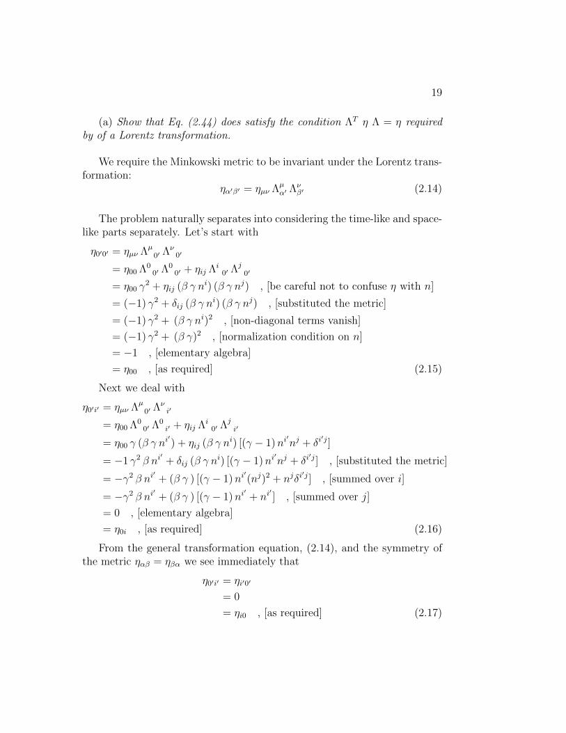
(a) Show that Eq. (2.44) does satisfy the condition ΛT η Λ = η requiredby of a Lorentz transformation.

We require the Minkowski metric to be invariant under the Lorentz trans-formation:

ηα′β′ = ηµν Λµα′ Λν

β′ (2.14)

The problem naturally separates into considering the time-like and space-like parts separately. Let’s start with

η0′0′ = ηµν Λµ0′ Λν

0′

= η00 Λ00′ Λ0

0′ + ηij Λi0′ Λj

0′

= η00 γ2 + ηij (β γ ni) (β γ nj) , [be careful not to confuse η with n]

= (−1) γ2 + δij (β γ ni) (β γ nj) , [substituted the metric]

= (−1) γ2 + (β γ ni)2 , [non-diagonal terms vanish]

= (−1) γ2 + (β γ)2 , [normalization condition on n]

= −1 , [elementary algebra]

= η00 , [as required] (2.15)

Next we deal with

η0′i′ = ηµν Λµ0′ Λν

i′

= η00 Λ00′ Λ0

i′ + ηij Λi0′ Λj

i′

= η00 γ (β γ ni′) + ηij (β γ ni) [(γ − 1)ni

′nj + δi

′j]

= −1 γ2 β ni′+ δij (β γ ni) [(γ − 1)ni

′nj + δi

′j] , [substituted the metric]

= −γ2 β ni′ + (β γ ) [(γ − 1)ni′(nj)2 + njδi

′j] , [summed over i]

= −γ2 β ni′ + (β γ ) [(γ − 1)ni′+ ni

′] , [summed over j]

= 0 , [elementary algebra]

= η0i , [as required] (2.16)

From the general transformation equation, (2.14), and the symmetry ofthe metric ηαβ = ηβα we see immediately that

η0′i′ = ηi′0′

= 0

= ηi0 , [as required] (2.17)

20

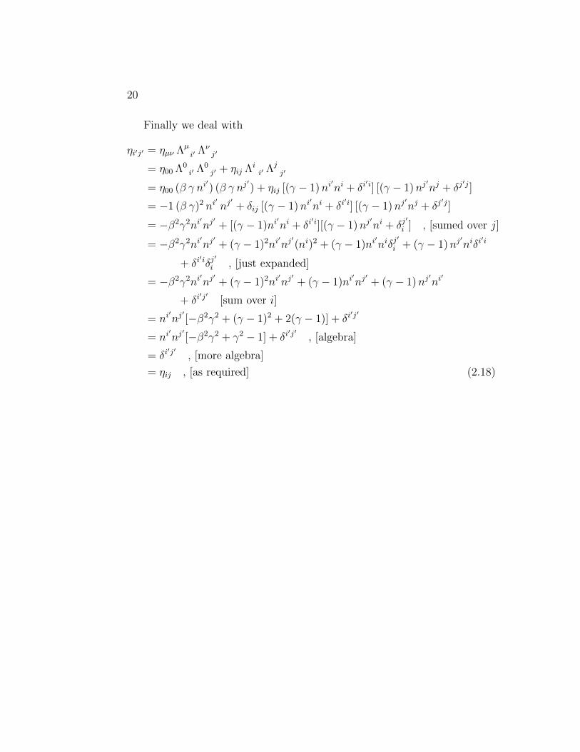
Finally we deal with

ηi′j′ = ηµν Λµi′ Λν

j′

= η00 Λ0i′ Λ0

j′ + ηij Λii′ Λj

j′

= η00 (β γ ni′) (β γ nj

′) + ηij [(γ − 1)ni

′ni + δi

′i] [(γ − 1)nj′nj + δj

′j]

= −1 (β γ)2 ni′nj

′+ δij [(γ − 1)ni

′ni + δi

′i] [(γ − 1)nj′nj + δj

′j]

= −β2γ2ni′nj

′+ [(γ − 1)ni

′ni + δi

′i][(γ − 1)nj′ni + δj

′

i ] , [sumed over j]

= −β2γ2ni′nj

′+ (γ − 1)2ni

′nj

′(ni)2 + (γ − 1)ni

′niδj

′

i + (γ − 1)nj′niδi

′i

+ δi′iδj

′

i , [just expanded]

= −β2γ2ni′nj

′+ (γ − 1)2ni

′nj

′+ (γ − 1)ni

′nj

′+ (γ − 1)nj

′ni

′

+ δi′j′ [sum over i]

= ni′nj

′[−β2γ2 + (γ − 1)2 + 2(γ − 1)] + δi

′j′

= ni′nj

′[−β2γ2 + γ2 − 1] + δi

′j′ , [algebra]

= δi′j′ , [more algebra]

= ηij , [as required] (2.18)

Chapter 3

The Electromagnetic Field

3.1 The Lorentz Force and the Electromag-

netic Field Tensor

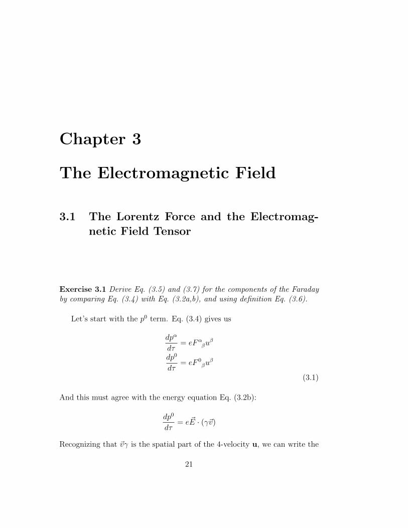
Exercise 3.1 Derive Eq. (3.5) and (3.7) for the components of the Faradayby comparing Eq. (3.4) with Eq. (3.2a,b), and using definition Eq. (3.6).

Let’s start with the p0 term. Eq. (3.4) gives us

dpα

dτ= eFα

βuβ

dp0

dτ= eF 0

βuβ

(3.1)

And this must agree with the energy equation Eq. (3.2b):

dp0

dτ= e ~E · (γ~v)

Recognizing that ~vγ is the spatial part of the 4-velocity u, we can write the

21

22

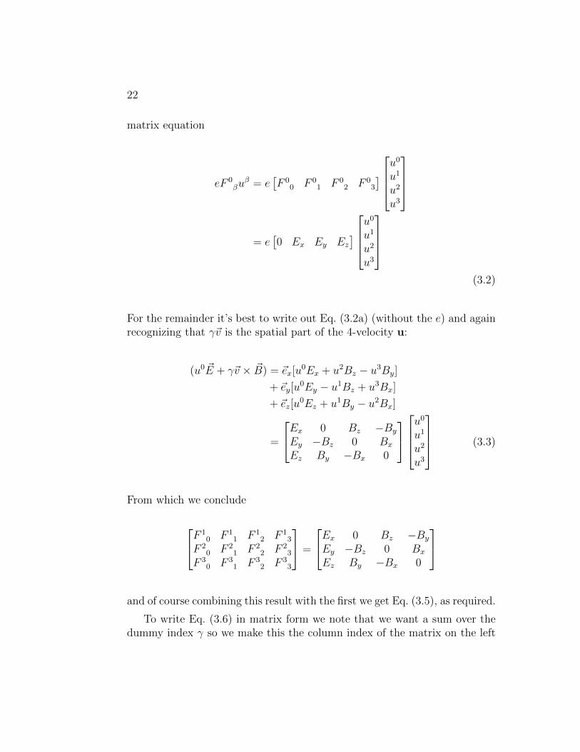
matrix equation

eF 0βu

β = e[F 0

0 F 01 F 0

2 F 03

] u0

u1

u2

u3

= e[0 Ex Ey Ez

] u0

u1

u2

u3

(3.2)

For the remainder it’s best to write out Eq. (3.2a) (without the e) and againrecognizing that γ~v is the spatial part of the 4-velocity u:

(u0 ~E + γ~v × ~B) = ~ex[u0Ex + u2Bz − u3By]

+ ~ey[u0Ey − u1Bz + u3Bx]

+ ~ez[u0Ez + u1By − u2Bx]

=

Ex 0 Bz −By

Ey −Bz 0 Bx

Ez By −Bx 0

u0

u1

u2

u3

(3.3)

From which we conclude

F 10 F 1

1 F 12 F 1

3

F 20 F 2

1 F 22 F 2

3

F 30 F 3

1 F 32 F 3

3

=

Ex 0 Bz −By

Ey −Bz 0 Bx

Ez By −Bx 0

and of course combining this result with the first we get Eq. (3.5), as required.

To write Eq. (3.6) in matrix form we note that we want a sum over thedummy index γ so we make this the column index of the matrix on the left

23

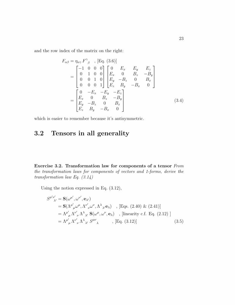
and the row index of the matrix on the right:

Fαβ = ηαγ Fγβ , [Eq. (3.6)]

=

−1 0 0 00 1 0 00 0 1 00 0 0 1

0 Ex Ey EzEx 0 Bz −By

Ey −Bz 0 Bx

Ez By −Bx 0

=

0 −Ex −Ey −EzEx 0 Bz −By

Ey −Bz 0 Bx

Ez By −Bx 0

(3.4)

which is easier to remember because it’s antisymmetric.

3.2 Tensors in all generality

Exercise 3.2. Transformation law for components of a tensor Fromthe transformation laws for components of vectors and 1-forms, derive thetransformation law Eq. (3.14)

Using the notion expressed in Eq. (3.12),

Sµ′ν′

λ′ = S(ωµ′, ων

′, eλ′)

= S(Λµ′

µωµ,Λν′

νων ,Λλ

λ′eλ) , [Eqs. (2.40) & (2.41)]

= Λµ′

µ Λν′

ν Λλλ′ S(ωµ, ων , eλ) , [linearity c.f. Eq. (2.12) ]

= Λµ′

µ Λν′

ν Λλλ′ S

µνλ , [Eq. (3.12)] (3.5)

24

Bibliography

Eisberg, R., and R. Resnick, 1985: Quantum Physics of atoms, molecules,solids, nuclei, and particles . 2nd ed., John Wiley and Sons, 713 pp.

Faber, R. L., 1983: Differential geometry and relativity theory: An Introduc-tion. Marcel Dekker. 255 + X pp.

Hobson, M., G. Efstathiou, and A. Lasenby, 2009: General Relativity: Anintroduction for physicists . Cambridge. 572 +XVIII pp.

Misner, C. W., K. S. Thorne, and J. A. Wheeler, 1973: Gravitation. W. H.Freeman and company. 1279 + XXVI pp.

25