GRAVITATION EFFECTS ON CENTRIFUGAL PENDULUM VIBRATION ABSORBERSLINEAR ANALYSIS

By

Ming Mu

A THESIS

Submittedto Michigan State University

in partial fulfillment of the requirementsfor the degree of

Mechanical Engineering – Master of Science

2015

ABSTRACT

GRAVITATION EFFECTS ON CENTRIFUGAL PENDULUM VIBRATION ABSORBERSLINEAR ANALYSIS

By

Ming Mu

This work investigates the effects of gravity on the dynamic response of centrifugal pendulum

vibration absorbers (CPVAs). This analytical study considers small amplitude motions of the ab-

sorbers so that linear vibration tools can be applied. The motivation of the study is to determine the

behavior of CPVAs at low rotor speeds, where gravity effects can be comparable to those of rota-

tion. The main goal of the present study is to predict patterns that were observed in the response of

systems with several symmetrically placed absorbers [10], and to use more sophisticated analysis

tools for symmetric systems, namely circulant matrices, to investigate the linearized version of the

model. A mathematical model is developed using Lagrange’s equations for a disk rotating about

a fixed horizontal axis and N point masses cyclically arranged on the rotor that can move along

paths relative to the rotor. Gravity provides both direct and parametric excitation to these pendu-

lum masses at order one, whereas the torque applied to the rotor is at order n. The equations are

linearized and non-dimensionalized for analysis. The number of distinct groups of absorbers with

identical but phase-shifted waveforms is considered, and it is shown that this grouping behavior

depends on the engine order n and the ratio Nn . Models with and without the effects of parametric

excitation are considered, and it is shown that parametric excitation leads to resonant effects when

n = 1 and n = 2. It is shown that the rotor is affected only by the order n component of the absorber

responses, because of the symmetries of the response at order one from gravity. These results pro-

vide useful information about absorber behavior and can be used to assess potential problems that

may arise from gravitational effects.

Copyright byMING MU

2015

To my wonderful family and all my friends.

iv

ACKNOWLEDGEMENTS

First of all, I would like to express my appreciations to all the people who have provided me

invaluable supports during my work on this thesis, especially my advisor, Dr. Steven W. Shaw, and

Dr. Brian Feeny, for giving me the opportunity to work on this project. I am very grateful for the

continuous support and guidance from Dr. Shaw to allow me continuing my education and work

over the last two and a half years. In addition, I would like to thank Bruce Geist.

Special thanks to Fiat Chrysler Automobiles, the National Science Foundation, and Michigan

State University for their support of my research.

I am also grateful to my labmates, Mustafa Ali Acar, Michael Thelen and many others for all

the endless discussions and lab works together.

Last but not the least, I would like to thank all my family members for their supports throughout

writing my thesis and my life in general.

v

TABLE OF CONTENTS

LIST OF TABLES . . . . . . . . . . . . . . . . . . . . . . . . . . . . . . . . . . . . . . . vii

LIST OF FIGURES . . . . . . . . . . . . . . . . . . . . . . . . . . . . . . . . . . . . . . . viii

CHAPTER 1 INTRODUCTION . . . . . . . . . . . . . . . . . . . . . . . . . . . . . . . 11.1 Background and Motivation . . . . . . . . . . . . . . . . . . . . . . . . . . . . . . 11.2 Thesis Outline . . . . . . . . . . . . . . . . . . . . . . . . . . . . . . . . . . . . . 3

CHAPTER 2 MATHEMATICAL MODELING . . . . . . . . . . . . . . . . . . . . . . . 52.1 Equations of Motion . . . . . . . . . . . . . . . . . . . . . . . . . . . . . . . . . . 52.2 Nondimensionalization and Linearization . . . . . . . . . . . . . . . . . . . . . . 72.3 Grouping Behavior Analysis . . . . . . . . . . . . . . . . . . . . . . . . . . . . . 11

CHAPTER 3 LINEAR MODEL WITHOUT PARAMETRIC EXCITATION . . . . . . . 153.1 Steady-state Damped Response . . . . . . . . . . . . . . . . . . . . . . . . . . . . 153.2 Diagonalization and Steady-State Solution . . . . . . . . . . . . . . . . . . . . . . 173.3 Steady-state Undamped Response . . . . . . . . . . . . . . . . . . . . . . . . . . 20

CHAPTER 4 ACCOUNTING FOR GRAVITATIONAL PARAMETRIC EXCITATION- PERTURBATION ANALYSIS . . . . . . . . . . . . . . . . . . . . . . . . 22

4.1 Scaling . . . . . . . . . . . . . . . . . . . . . . . . . . . . . . . . . . . . . . . . . 224.2 Single Absorber Case . . . . . . . . . . . . . . . . . . . . . . . . . . . . . . . . . 224.3 Multiple Absorbers Case . . . . . . . . . . . . . . . . . . . . . . . . . . . . . . . 254.4 Slow Flow in Cartesian Coordinates . . . . . . . . . . . . . . . . . . . . . . . . . 274.5 Analysis with Damping Effects . . . . . . . . . . . . . . . . . . . . . . . . . . . . 314.6 Rotor Behavior Analysis . . . . . . . . . . . . . . . . . . . . . . . . . . . . . . . 344.7 Results and Discussions . . . . . . . . . . . . . . . . . . . . . . . . . . . . . . . . 35

CHAPTER 5 CONCLUSIONS AND FUTURE WORK . . . . . . . . . . . . . . . . . . . 465.1 Summary and Conclusions . . . . . . . . . . . . . . . . . . . . . . . . . . . . . . 465.2 Recommendations for Future Work . . . . . . . . . . . . . . . . . . . . . . . . . . 48

BIBLIOGRAPHY . . . . . . . . . . . . . . . . . . . . . . . . . . . . . . . . . . . . . . . . 50

vi

LIST OF TABLES

Table 2.1: Symbols and descriptions from Figure 2.1. . . . . . . . . . . . . . . . . . . . . 6

Table 2.2: Path functions from Denman [2]. . . . . . . . . . . . . . . . . . . . . . . . . . . 9

Table 2.3: Path variables and required expansions. . . . . . . . . . . . . . . . . . . . . . . 9

Table 2.4: Examples of l, k and q with different values of N and n. . . . . . . . . . . . . . . 13

Table 2.5: Number of groups with different values of N and n. . . . . . . . . . . . . . . . . 14

Table 2.6: Summary of grouping with different N and n . . . . . . . . . . . . . . . . . . . 14

vii

LIST OF FIGURES

Figure 1.1: Bifilar design of CPVA. . . . . . . . . . . . . . . . . . . . . . . . . . . . . . . 2

Figure 2.1: Modeling diagram. . . . . . . . . . . . . . . . . . . . . . . . . . . . . . . . . 5

Figure 2.2: Layout of ith and jth absorber. . . . . . . . . . . . . . . . . . . . . . . . . . . 12

Figure 3.1: Steady-state response peak amplitudes of a system of N CPVAs with increas-ing torque amplitude Γθ ; for γ = 0.05, with damping. . . . . . . . . . . . . . . 20

Figure 4.1: Steady-state response amplitudes of a single (N = 1) CPVA with increasingtorque, Γθ ; for γ = 0.05, n = 2, µa = 0.04, and σ = 0. . . . . . . . . . . . . . . 36

Figure 4.2: Steady-state response amplitudes of a single (N = 1) CPVA time-trace plotat various torque level, for γ = 0.05, n = 2, µa = 0.04, and σ = 0. . . . . . . . 37

Figure 4.3: Steady-state response amplitudes of a single (N = 1) CPVA with increasingtorque, Γθ ; for γ = 0.05, n = 1.5, µa = 0.03, and σ = 0. . . . . . . . . . . . . . 38

Figure 4.4: Damped, µa = 0.04, versus undamped steady-state response amplitude of 1CPVA with increasing Γθ , γ = 0.05, n = 2 with σ = 0. . . . . . . . . . . . . . 39

Figure 4.5: Damped, µa = 0.03, versus undamped steady-state response amplitude of 1CPVA with increasing Γθ , γ = 0.05, n = 1.5 with σ = 0. . . . . . . . . . . . . 40

Figure 4.6: Steady-state time traces of 4 CPVAs, Γθ = 0.01, γ = 0.05, n = 2, with µa =0.04 and σ = 0. . . . . . . . . . . . . . . . . . . . . . . . . . . . . . . . . . . 40

Figure 4.7: Steady-state response amplitudes of 4 CPVAs with increasing Γθ , γ = 0.05,n = 2, with µa = 0.04 and σ = 0. . . . . . . . . . . . . . . . . . . . . . . . . . 41

Figure 4.8: Steady-state time traces of 4 CPVAs, Γθ = 0.01, γ = 0.05, n = 1.5, withµa = 0.03 and σ = 0. . . . . . . . . . . . . . . . . . . . . . . . . . . . . . . . 41

Figure 4.9: Steady-state response amplitudes of 4 CPVAs with increasing Γθ , γ = 0.05,n = 1.5, with µa = 0.03 and σ = 0. . . . . . . . . . . . . . . . . . . . . . . . . 42

Figure 4.10: Steady-state response peak amplitudes plots of 4 CPVAs between non-linearsimulation, linear simulation and analysis, with increasing Γθ , γ = 0.05, n =1.5, with µa = 0.03 and σ = 0. . . . . . . . . . . . . . . . . . . . . . . . . . . 42

Figure 4.11: Damped vs undamped steady-state response amplitudes of 4 CPVAs withincreasing Γθ , γ = 0.05, n = 2 with σ = 0.02. . . . . . . . . . . . . . . . . . . 43

viii

Figure 4.12: Rotor peak amplitude plot with 4 CPVAs with increasing Γθ , γ = 0.05, n =1.5 with σ = 0, analysis versus nonlinear simulation. . . . . . . . . . . . . . . 44

Figure 4.13: Rotor peak amplitude plot with 4 CPVAs with increasing Γθ , γ = 0.05, n = 2with σ = 0, analysis versus linear simulation. . . . . . . . . . . . . . . . . . . 45

Figure 5.1: Nonlinear simul rotor peak amplitude plot with 4 CPVAs with increasing Γθ ,γ = 0.05, n = 2 with 0 detuning. . . . . . . . . . . . . . . . . . . . . . . . . . 49

ix

CHAPTER 1

INTRODUCTION

1.1 Background and Motivation

Torsional vibration is a major concern in power transmission systems that have rotating compo-

nents such as shafts or couplings. Not only can torsional vibration compromise the integrity of the

structure of those components, it can also affect the performance and robustness of other mechani-

cal parts either directly or indirectly, producing noise, or in the worst case, system failure. Ideally,

the torque will be generated and transmitted "smoothly" throughout the whole system, thus ensur-

ing that the rotational speed is constant. However, in reality, the generated torque is usually not

smooth, but has fluctuations, and often these are order based, that is, their frequency is proportional

to the rotation rate. A common example of this is in internal combustion engines, where the in-

cylinder gas pressure varies substantially over each cycle [9]. In a four-stroke engine the excitation

order is the half of the number of cylinders, since each cylinder fires ones per two revolutions of

the crank. Additionally, the connected parts such as reduction gears, drive shafts, couplings, etc.,

can increase torsional vibration. These vibrations usually appear throughout the whole operating

range at all operating speeds, and cause particular problems in resonance conditions.

Traditional methods that have been used to mitigate torsional vibration in internal combustion

engines include the use of torsional friction dampers, large inertia flywheels, and so-called har-

monic balancers, which are simply frequency tuned torsional vibration absorbers. However, those

methods have trade-offs such as engine performance, engine efficiency, and limited speed range.

Another solution to reduce torsional vibrations is by adding order-tuned vibration absorbers,

namely, centrifugal pendulum vibration absorbers (CPVAs). The CPVA was first utilized in geared

radial aircraft-engine-propeller systems during World War II [12]. Early designs of CPVAs used a

circle for the path followed by the center of mass of the absorbers, due to the ease of manufacture

1

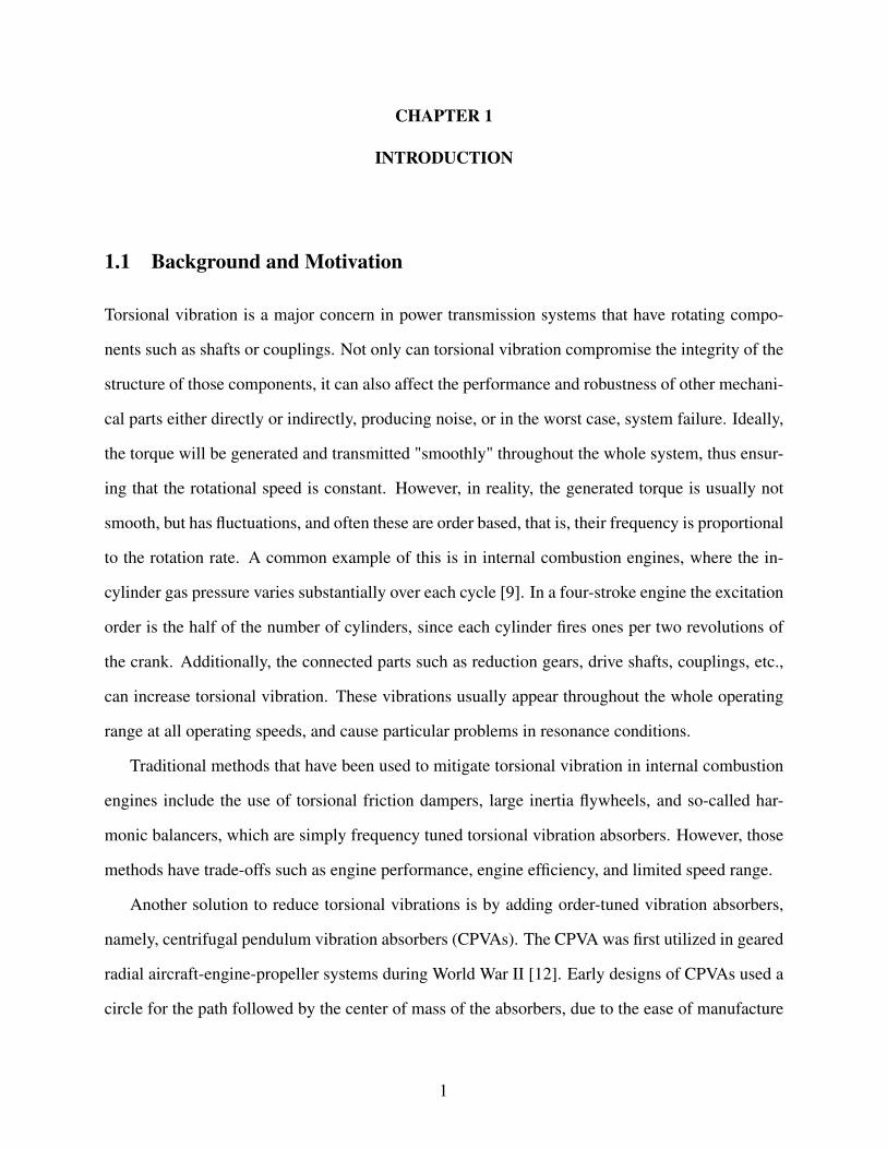
and the use of bifilar (two point) suspensions for the absorber mass, which is convenient design be-

cause of its compactness (see Figure 1.1). However, Newland [6] showed an instability could arise

from nonlinear effects, resulting in a jump in phase that made the CPVA into a vibration amplifier.

The traditional remedy for this was to overtune the absorbers, which enhanced robustness at the

expense of performance. Later, this led to the development of alternative paths that circumvent,

to a large extent, this nonlinear behavior. Along these lines, Madden [3] patented the bifilar sus-

pension absorber design with a cycloidal path, similar to that shown in Figure 1.1, for application

to helicopter rotors. Later, Denman [2] introduced the tautochronic path, which makes the tuning

order constant at all amplitudes. He also built a model that included the influence from the rollers

used in the bifilar suspension.

Figure 1.1: Bifilar design of CPVA.

The main advantage of a CPVA is that it is driven by the centrifugal forces and torsional vibra-

tions, so it does not require extra energy input and acts as a passive device. The CPVA’s natural

frequency is proportional to the mean rotating speed of the crankshaft, which plays an essential

role in their tuning. The constant ratio is called the absorber order, which is set by its design pa-

rameters, specifically, the radius of the holes and rollers in the bifilar design, and can be tuned to

match the engine excitation order. Automotive companies have recently been doing research on the

implementation of CPVAs in car engines and other powertrain components because they believe

CPVAs will help decrease fuel consumption by reducing torsional vibrations, thereby allowing en-

2

gines to run at lower speeds, where pumping losses are reduced [5, 1]. In fact, CPVAs are already

in production for use in torque converters and dual mass flywheels [8].

However, a concern when implementing CPVAs in engines is that the rotational axis is hori-

zontal and, thus, the rotating plane is vertical, thereby causing gravitational forces to act on the

rotor-absorber system in addition to the engine torque. In fact, these effects come into play at low

engine speeds, in particular, at idle. The interplay of gravity, which has order one (one cycle of

forcing per revolution) and subjects the absorbers to both direct and parametric excitation, and the

order n engine torque acting on the rotor, can have interesting consequences, as described below.

An investigation of the general effects of gravity on the dynamics of CPVA systems with mul-

tiple absorbers placed cyclically around a rotor was done by T. Theisen [10], who used the method

of multiple scales to investigate the nonlinear response of CPVA systems with gravity. One of the

results from Theisen’s work shows that with different engine orders and number of absorbers, in

some cases the absorbers all behave identically, with a phase shift due to their placement around

the rotor, but in other cases they behave differently. This so-called grouping behavior was observed

and analyzed in terms of possible resonance conditions, but not examined from a general point of

view. The present work was motivated by Theisen’s results, with a goal of understanding the role

of the gravitational parametric excitation, to take advantage of some of the special properties of

cyclic systems, and to uncover the fundamental reasons behind the observed grouping behavior.

These goals can be met by considering the linearized equations of motion which are valid for small

absorber amplitudes, and that is the model used in the present study.

1.2 Thesis Outline

The remainder of this thesis is arranged as follows: In Chapter 2, the mathematical modeling for

a rotor/absorber system is conducted, and the nonlinear equations of motion (EOM) with gravity

terms are obtained by using Lagrange’s equation. Then, a linearization version of the EOMs is

obtained by assuming small absorber motions and small rotor speed fluctuations. In previous

works several different types of absorber paths are considered, but in the linear theory only the

3

small amplitude absorber tuning affects the equations, as the movement of absorbers is assumed to

be small. At the end of Chapter 2 we anticipate what the form of the absorber response, in terms of

its harmonic content, and use that form to derive a general theory for the grouping results observed

by Theisen, which are confirmed in this work. In Chapter 3, a preliminary study is considered

in which the parametric term, that is, the time-varying gravity stiffness term, is omitted, giving

a simple model that provides insight for the rest of the investigation. In this analysis, the rotor

equation is expanded and substituted into the absorber equations, and the latter are transformed

into matrix form. Since the parametric term is omitted, it is easy to perform diagnolization of the

system by introducing Fourier matrices, as the coefficient matrices are circulant [7], and an exact

form for the steady-state solutions is found. In Chapter 4, a perturbation analysis is performed

to the linear equations in which the parametric term from gravity is included. The equations are

scaled so that the Method of Multiple Scales can be used. From the scaled linear equations, there

is only one special case (engine order n = 2) in which the absorbers resonantly interact with the

parametric excitation from gravity and the applied torque. The analysis in this chapter is first done

without damping for simplicity, after which the effects of damping are considered. In the last part

of this chapter, the rotor behavior is recovered and analyzed using the solutions from the analysis

of the absorber response. The results are shown in the form of plots for some specific cases that

may be of interest for industrial applications. The analytical results are compared with numerical

simulations of the linear and nonlinear equations of motion, and good agreement is found. Chapter

5 provides the conclusions of this thesis and outlines future work on this topic.

4

CHAPTER 2

MATHEMATICAL MODELING

2.1 Equations of Motion

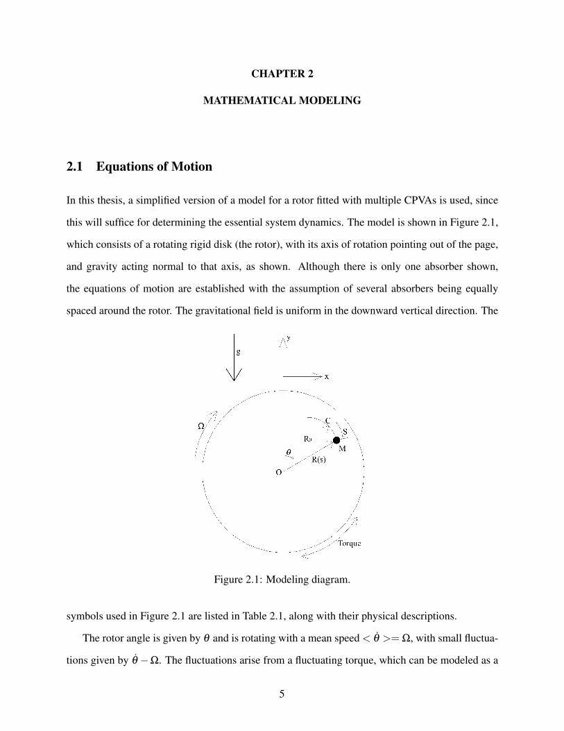
In this thesis, a simplified version of a model for a rotor fitted with multiple CPVAs is used, since

this will suffice for determining the essential system dynamics. The model is shown in Figure 2.1,

which consists of a rotating rigid disk (the rotor), with its axis of rotation pointing out of the page,

and gravity acting normal to that axis, as shown. Although there is only one absorber shown,

the equations of motion are established with the assumption of several absorbers being equally

spaced around the rotor. The gravitational field is uniform in the downward vertical direction. The

Figure 2.1: Modeling diagram.

symbols used in Figure 2.1 are listed in Table 2.1, along with their physical descriptions.

The rotor angle is given by θ and is rotating with a mean speed < θ >= Ω, with small fluctua-

tions given by θ −Ω. The fluctuations arise from a fluctuating torque, which can be modeled as a

5

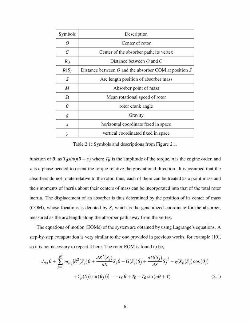
Symbols Description

O Center of rotor

C Center of the absorber path; its vertex

R0 Distance between O and C

R(S) Distance between O and the absorber COM at position S

S Arc length position of absorber mass

M Absorber point of mass

Ω Mean rotational speed of rotor

θ rotor crank angle

g Gravity

x horizontal coordinate fixed in space

y vertical coordinated fixed in space

Table 2.1: Symbols and descriptions from Figure 2.1.

function of θ , as Tθ sin(nθ + τ) where Tθ is the amplitude of the torque, n is the engine order, and

τ is a phase needed to orient the torque relative the graviational direction. It is assumed that the

absorbers do not rotate relative to the rotor, thus, each of them can be treated as a point mass and

their moments of inertia about their centers of mass can be incorporated into that of the total rotor

inertia. The displacement of an absorber is thus determined by the position of its center of mass

(COM), whose locations is denoted by S, which is the generalized coordinate for the absorber,

measured as the arc length along the absorber path away from the vertex.

The equations of motion (EOMs) of the system are obtained by using Lagrange’s equations. A

step-by-step computation is very similar to the one provided in previous works, for example [10],

so it is not necessary to repeat it here. The rotor EOM is found to be,

Jrot θ +N

∑j=1

mp j[R2(S j)θ +

dR2(S j)

dSS jθ +G(S j)S j +

dG(S j)

dSS j

2−g(Xp(S j)cos(θ j)

+Yp(S j)sin(θ j))] =−c0θ +T0 +Tθ sin(nθ + τ) (2.1)

6

and the EOM for the jth absorber is expressed as,

mp j[S j +G(S j)θ −12

dR2(S j)

dSθ

2 +g(−dXp(S j)

dSsin(θ j)+

dYp(S j)

dScos(θ j))]

=−ca jS j (2.2)

where mp j is mass of the jth absorber, Jrot is the rotor moment of inertia, Xp and Yp are the x and y

components of the location of R(S j), ca j is the damping coefficient for the jth absorber, and G(S j)

is a function of the path, given by

G(S j) =

√R2(S j)−

14(dR2(S j)

dS)2,

which is a path function, represented as a part of kinetic energy. These equations are the basis for

the analysis and simulation of CPVA systems, however, they are fully nonlinear. A first step in

understanding the system dynamics is to consider the dynamics of the linearized model in which

the absorbers and rotor undergo small amplitude oscillations.

2.2 Nondimensionalization and Linearization

The EOMs are formulated in terms of time dependent generalized coordinates θ and the S js.

However, the fluctuating torque is a function of the rotor angle, θ , which is a monotonic function

of time, and so it is convenient to convert the independent variable from time to θ , which renders

the torque as a periodic excitation. This is done by first introducing non-dimensional variables ν

and ω as,

ν =θ

Ω= 1+ω (2.3)

where ν is the non-dimensional rotor speed and ω describes normalized speed fluctuations about

Ω, which are generally small, that is, |ω| << 1. We will express both ν and ω as functions of θ ,

rather than time.

7

The transformation from time dependent derivative to θ dependent derivative is done by using

the chain rule and using the definition of ν . This formulation for derivatives is given by

˙(∗) = d(∗)dt

=d(∗)dθ

dθ

dt=

d(∗)dθ

νΩ = Ων(∗)′ (2.4)

¨(∗) = d2(∗)dθ 2 (

dθ

dt)2 +

d(∗)dθ

(d2θ

dt2 ) = ν2Ω

2(∗)′′+νν′Ω

2(∗)′, (2.5)

so that the primes are dimensionless derivatives.

By using Equation 2.4 above, Equation 2.1 and Equation 2.2 are transformed as

JrotΩ2νν′+

N

∑j=1

mp j[R2(S j)Ω

2νν′+

dR2(S j)

dSν

2Ω

2S j′+G(S j)[ν

2Ω

2S j′′+Ω

2νν′S j′]

+dG(S j)

dSν

2Ω

2S j′2−g(Xp(S j)cos(θ j)

+Yp(S j)sin(θ j))] =−c0νΩ+T0 +Tθ sin(nθ + τ) (2.6)

mp j[ν2Ω

2S j′′+Ω

2νν′S j′+G(S j)Ω

2νν

2− 12

dR2(S j)

dSΩ

2ν

2

+g(−dXp(S j)

dSsin(θ j)+

dYp(S j)

dScos(θ j))] =−ca jνΩS j

′ (2.7)

which represent the fully nonlinear equations expressed with θ as the independent variable.

To formulate the EOM one must specify the path of the absorber, which is captured in the

function R(S), which then dictates X(S),Y (S),G(S). The details of different path formulations can

be found in Denman’s work [2], but here only the small amplitude nature of the path is important,

namely the curvature at the vertex. The parameters and their expressions are given in Table 2.2,

as functions of the arc-length variable S, where ρ0 is path radius of curvature at the vertex (that

is, at S = 0), λ ∈ [0,1] is a characteristic parameter dictating the nonlinear nature of the path,

and the angle Φ j is an effective angular position of absorber j from its vertex, given by Φ j =

1λ

arcsin(

λS jρ0

)[2, 10]. Note that the radius of curvature ρ0 dictates the small amplitude (linear)

absorber tuning order, n, which is purely geometry-dependent and given by the relation

ρ0 =R0

n2 +1

8

Term Nonlinear Expression from Denman

Xp(S j)ρ0

1−λ2 (sin(Φ j)cos(λΦ j)−λ2S j

ρ0cos(Φ j))

Yp(S j) R0 +ρ0

1−λ2 (cos(Φ j)cos(λΦ j)+λ2S j

ρ0sin(Φ j)−1)

R2(S j) Xp2 +Yp

2

G(S j)

√R2(S j)− 1

4(DR2(S j)

DS) )2

Table 2.2: Path functions from Denman [2].

To proceed with linearization of the EOM we first nondimensionalize the absorber variable by

defining s j =S jR0

, and note that |s j| << 1 for realistic motions. Therefore, terms that depends on

s j are linearized by keeping only the constant and linear terms from their Taylor series expansions

about s j = 0. Also, since νν ′ = (1+ω)ω ′ where ω is assumed small, it follows that νν ′=ω ′

and ν2=1+ 2ω . Terms involving νν ′s′, s′2, and other products of small terms are ignored. The

linearized and non-dimensionalized parameters are listed in Table 2.3. Note that derivatives of

some terms are needed in the EOM, so that quadratic terms in some expansions are reserved.

Non-dim. Term Definition Required Expansion

xp(s j)Xp(S j)

R0s

yp(s j)Yp(S j)

R01− 1

2(1+ n2)s j2

r2(s j) xp2 + xp

2 1− n2s j2

g(s j)G(S j)

R01− 1

2(n2 + n4)s j

2

Table 2.3: Path variables and required expansions.

With these expressions, the non-dimensional version of the derivatives needed in the EOM can

9

be expressed as

dxp(s j)

ds=1

dyp(s j)

ds=− (1+ n2)s j

dr2(Ss j)

ds=−2n2s j

dg(s j)

ds=− (n2 + n4)s j

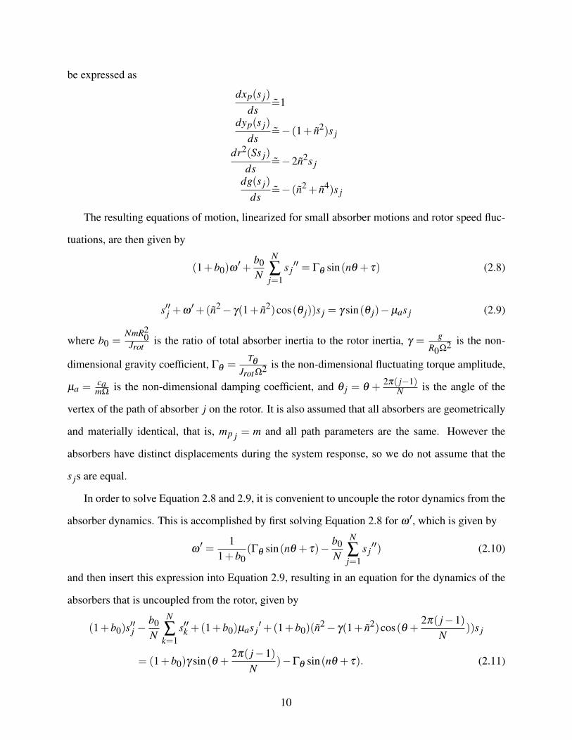
The resulting equations of motion, linearized for small absorber motions and rotor speed fluc-

tuations, are then given by

(1+b0)ω′+

b0N

N

∑j=1

s j′′ = Γθ sin(nθ + τ) (2.8)

s′′j +ω′+(n2− γ(1+ n2)cos(θ j))s j = γ sin(θ j)−µas j (2.9)

where b0 =NmR2

0Jrot

is the ratio of total absorber inertia to the rotor inertia, γ = gR0Ω2 is the non-

dimensional gravity coefficient, Γθ =Tθ

JrotΩ2 is the non-dimensional fluctuating torque amplitude,

µa = camΩ

is the non-dimensional damping coefficient, and θ j = θ +2π( j−1)

N is the angle of the

vertex of the path of absorber j on the rotor. It is also assumed that all absorbers are geometrically

and materially identical, that is, mp j = m and all path parameters are the same. However the

absorbers have distinct displacements during the system response, so we do not assume that the

s js are equal.

In order to solve Equation 2.8 and 2.9, it is convenient to uncouple the rotor dynamics from the

absorber dynamics. This is accomplished by first solving Equation 2.8 for ω ′, which is given by

ω′ =

11+b0

(Γθ sin(nθ + τ)− b0N

N

∑j=1

s j′′) (2.10)

and then insert this expression into Equation 2.9, resulting in an equation for the dynamics of the

absorbers that is uncoupled from the rotor, given by

(1+b0)s′′j −

b0N

N

∑k=1

s′′k +(1+b0)µas j′+(1+b0)(n

2− γ(1+ n2)cos(θ +2π( j−1)

N))s j

= (1+b0)γ sin(θ +2π( j−1)

N)−Γθ sin(nθ + τ). (2.11)

10

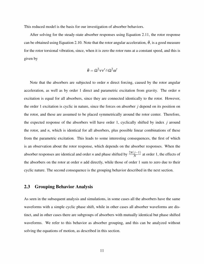
This reduced model is the basis for our investigation of absorber behaviors.

After solving for the steady-state absorber responses using Equation 2.11, the rotor response

can be obtained using Equation 2.10. Note that the rotor angular acceleration, θ , is a good measure

for the rotor torsional vibration, since, when it is zero the rotor runs at a constant speed, and this is

given by

θ = Ω2νν′=Ω

2ω′

Note that the absorbers are subjected to order n direct forcing, caused by the rotor angular

acceleration, as well as by order 1 direct and parametric excitation from gravity. The order n

excitation is equal for all absorbers, since they are connected identically to the rotor. However,

the order 1 excitation is cyclic in nature, since the forces on absorber j depend on its position on

the rotor, and these are assumed to be placed symmetrically around the rotor center. Therefore,

the expected response of the absorbers will have order 1, cyclically shifted by index j around

the rotor, and n, which is identical for all absorbers, plus possible linear combinations of these

from the parametric excitation. This leads to some interesting consequences, the first of which

is an observation about the rotor response, which depends on the absorber responses. When the

absorber responses are identical and order n and phase shifted by 2π( j−1)N at order 1, the effects of

the absorbers on the rotor at order n add directly, while those of order 1 sum to zero due to their

cyclic nature. The second consequence is the grouping behavior described in the next section.

2.3 Grouping Behavior Analysis

As seen in the subsequent analysis and simulations, in some cases all the absorbers have the same

waveforms with a simple cyclic phase shift, while in other cases all absorber waveforms are dis-

tinct, and in other cases there are subgroups of absorbers with mutually identical but phase shifted

waveforms. We refer to this behavior as absorber grouping, and this can be analyzed without

solving the equations of motion, as described in this section.

11

In order to predict which absorbers will group together, it is convenient to express the general

form of the response of the ith absorber, with a cyclic order 1 component of amplitude A and an

order n component of amplitude B, as

si(θ) = Asin(nθ + τ)+Bsin(θ +2π(i−1)

N) (2.12)

where τ accounts for the phase shift between the orders. We now consider another absorber, s j(θ),

where j = i+ l, that is, the absorber that is l sections away from the ith absorber, and express its

response as

s j(θ) = Asin(nθ + τ)+Bsin(θ +2π(i+ l−1)

N) (2.13)

noting that the order n response is the same for all absorbers and that the order one component is

phase shifted by the sector angle between the absorbers. Note that form holds for l = 1,2, ...,(N−

1).

Figure 2.2: Layout of ith and jth absorber.

We next consider the conditions under which the waveform of absorber j will be identical to

that of the i absorber, but with a different phase. To this end, we add a dummy phase ψ to both

components of absorber i and examine the conditions for which s j(θ) = si(θ +ψ). The following

expansion of si(θ +ψ) is used to compare it with s j:

si(θ +ψ) = Asin(nθ +nψ + τ)+Bsin(θ +2π(i−1)

N+ψ). (2.14)

12

Since there are two sine functions with different orders in the steady-state response of each ab-

sorber, in order to have s j and si equal, it is necessary to have nψ = 2πk, k = 1,2,3, ... and

ψ − 2πlN = 2πq, q = 1,2,3, .... Thus, the condition for identical absorber waveforms can be ex-

pressed by eliminating ψ from these two conditions, resulting in the following condition on l as a

function of indices k and q,

l =Nn(k−nq). (2.15)

For given number of absorbers, N, and engine order n, the waveforms of si and s j absorbers

will be identical if one can find integers l if k and q that satisfy this condition. Some examples are

shown in Table 2.4, where "-" means "no solution", which means the selected waveforms will be

different,

(a) N = 3, n = 2

l k q

1 - -

2 - -

(b) N = 4, n = 2

l k q

1 - -

2 3 1

3 - -

(c) N = 5, n = 2.5

l k q

1 3 1

2 6 2

3 4 1

4 7 2

(d) N = 6, n = 2

l k q

1 - -

2 - -

3 3 1

4 - -

5 - -

Table 2.4: Examples of l, k and q with different values of N and n.

In Table 2.4b, with N = 4 and n = 2, the only solution for l is l = 2, and therefore absorber

3 will have the same waveform as absorber 1, and from symmetry considerations absorbers 2 and

4 must also match, and so there are two groups of absorbers, which is seen in Figure 3.1b in the

next chapter; more about this follows below. In Table 2.4a, with N = 3 and n = 2, there is no

solution for any value of l, so that all absorbers have distinct responses and there are 3 (N) groups.

This corresponds to the case in Figure 3.1a in the next chapter. In Table 2.4c, with N = 5 and

n = 2.5, there is a solution to Equation 2.15 for every value of l, so that all absorbers have the same

waveform and there is only one absorber group. This corresponds to the case in Figure 3.1c in the

next chapter. In Table 2.4d, with N = 6 and n = 2, the only solution is for l = 3, so that absorbers 1

13

and 4 match, as do absorbers 2 and 5 and absorbers 3 and 6, that is, there are three absorber groups.

This is the case shown in Figure 3.1d in the next chapter.

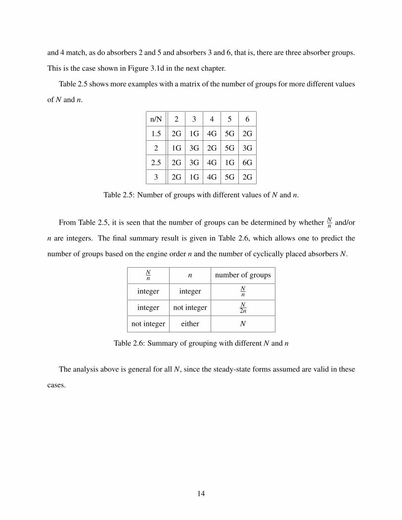
Table 2.5 shows more examples with a matrix of the number of groups for more different values

of N and n.

n/N 2 3 4 5 6

1.5 2G 1G 4G 5G 2G

2 1G 3G 2G 5G 3G

2.5 2G 3G 4G 1G 6G

3 2G 1G 4G 5G 2G

Table 2.5: Number of groups with different values of N and n.

From Table 2.5, it is seen that the number of groups can be determined by whether Nn and/or

n are integers. The final summary result is given in Table 2.6, which allows one to predict the

number of groups based on the engine order n and the number of cyclically placed absorbers N.

Nn n number of groups

integer integer Nn

integer not integer N2n

not integer either N

Table 2.6: Summary of grouping with different N and n

The analysis above is general for all N, since the steady-state forms assumed are valid in these

cases.

14

CHAPTER 3

LINEAR MODEL WITHOUT PARAMETRIC EXCITATION

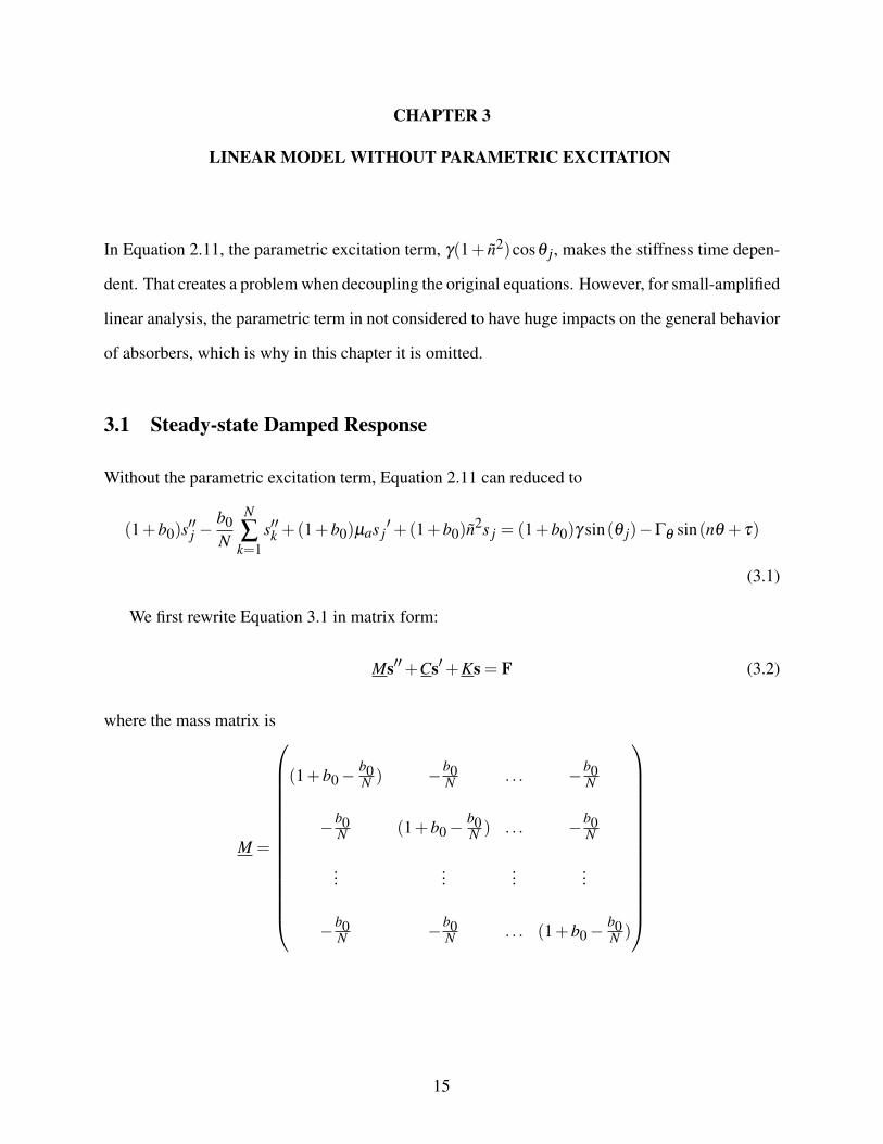
In Equation 2.11, the parametric excitation term, γ(1+ n2)cosθ j, makes the stiffness time depen-

dent. That creates a problem when decoupling the original equations. However, for small-amplified

linear analysis, the parametric term in not considered to have huge impacts on the general behavior

of absorbers, which is why in this chapter it is omitted.

3.1 Steady-state Damped Response

Without the parametric excitation term, Equation 2.11 can reduced to

(1+b0)s′′j −

b0N

N

∑k=1

s′′k +(1+b0)µas j′+(1+b0)n

2s j = (1+b0)γ sin(θ j)−Γθ sin(nθ + τ)

(3.1)

We first rewrite Equation 3.1 in matrix form:

Ms′′+Cs′+Ks = F (3.2)

where the mass matrix is

M =

(1+b0−b0N ) −b0

N . . . −b0N

−b0N (1+b0−

b0N ) . . . −b0

N

......

......

−b0N −b0

N . . . (1+b0−b0N )

15

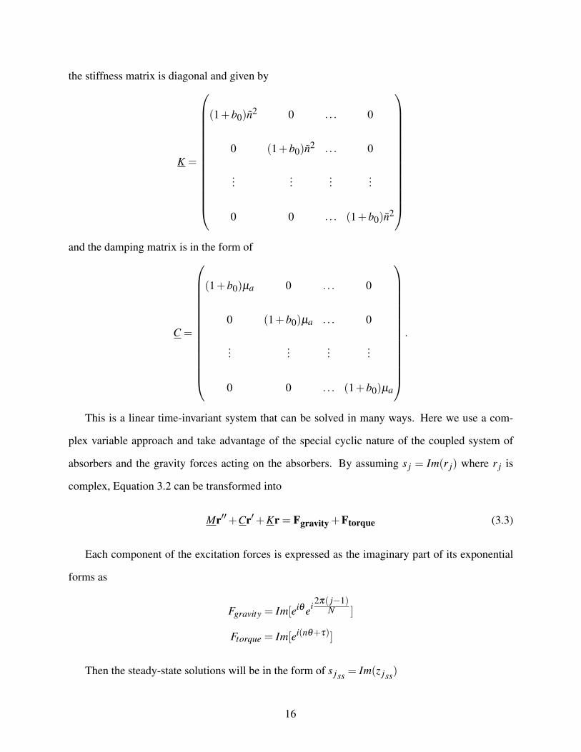
the stiffness matrix is diagonal and given by

K =

(1+b0)n2 0 . . . 0

0 (1+b0)n2 . . . 0

......

......

0 0 . . . (1+b0)n2

and the damping matrix is in the form of

C =

(1+b0)µa 0 . . . 0

0 (1+b0)µa . . . 0

......

......

0 0 . . . (1+b0)µa

.

This is a linear time-invariant system that can be solved in many ways. Here we use a com-

plex variable approach and take advantage of the special cyclic nature of the coupled system of

absorbers and the gravity forces acting on the absorbers. By assuming s j = Im(r j) where r j is

complex, Equation 3.2 can be transformed into

Mr′′+Cr′+Kr = Fgravity +Ftorque (3.3)

Each component of the excitation forces is expressed as the imaginary part of its exponential

forms as

Fgravity = Im[eiθ ei2π( j−1)N ]

Ftorque = Im[ei(nθ+τ)]

Then the steady-state solutions will be in the form of s jss = Im(z jss)

16

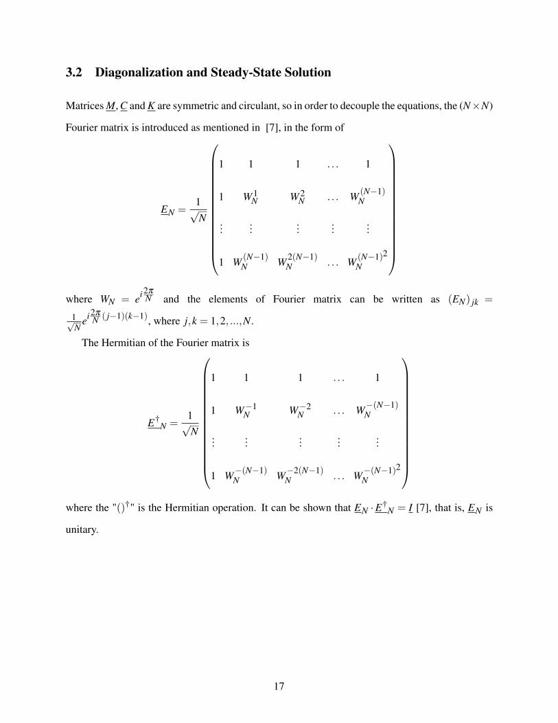
3.2 Diagonalization and Steady-State Solution

Matrices M, C and K are symmetric and circulant, so in order to decouple the equations, the (N×N)

Fourier matrix is introduced as mentioned in [7], in the form of

EN =1√N

1 1 1 . . . 1

1 W 1N W 2

N . . . W (N−1)N

......

......

...

1 W (N−1)N W 2(N−1)

N . . . W (N−1)2N

where WN = ei2π

N and the elements of Fourier matrix can be written as (EN) jk =

1√N

ei2πN ( j−1)(k−1), where j,k = 1,2, ...,N.

The Hermitian of the Fourier matrix is

E†N =

1√N

1 1 1 . . . 1

1 W−1N W−2

N . . . W−(N−1)N

......

......

...

1 W−(N−1)N W−2(N−1)

N . . . W−(N−1)2N

where the "()†" is the Hermitian operation. It can be shown that EN ·E†

N = I [7], that is, EN is

unitary.

17

Note that W N provides a convenient way to express the complex excitation force. Specifically,

F = (1+b0)γeiθ

1

W 1N

...

W (N−1)N

−Γθ ei(nθ+τ)

1

1

...

1

We define complex modal coordinates q for this system using EN as

r = ENq (3.4)

Substituting Equation 3.4 into Equation 3.3 and multipling the equation by E†N , we have,

E†NMENq′′+E†

NCENq′+E†NKENq = E†

NF (3.5)

which are uncoupled.

The diagonal stiffness and damping matrices are unchanged by this transformation, K =

E†NKEN = K and C = E†

NCEN =C. The diagonalized mass matrix is obtained as

M = E†NMEN =

1 0 . . . 0

0 (1+b0) . . . 0

......

......

0 0 . . . (1+b0)

.

18

The modal excitation term is given by E†NF as

E†NF = (1+b0)γeiθ√N

0

1

...

0

−Γθ ei(nθ+τ)

√N

1

0

...

0

which shows that, for these modal coordinates, gravity excites only the second mode and the

fluctuating torque excites only the first mode.

Thus, for steady-state study, there are only two modal equations that need to be solved, specif-

ically,

q′′1 +(1+b0)µaq1′+(1+b0)n

2q1 =−Γθ ei(nθ+τ)√

N (3.6)

q′′2 +(1+b0)µaq2′+ n2q2 = γeiθ√N (3.7)

The steady-state solutions in model coordinates are

q1s =

√Nei(nθ+τ)

n2− (1+b0)n2− inµa(1+b0)Γθ (3.8)

q2s =

√Neiθ

n2−1+ iµaγ (3.9)

Then, the steady-state solution in original coordinates, ss, is obtained by multiplying qs by the

Fourier matrix, EN , and taking the imaginary parts of the result.

Figure 3.1 shows the absorber steady-state response peak amplitudes with increasing torque for

several sample cases.

As can be seen in Figure 3.1, for some given N and n, some absorbers, or in some case all of

them, have the same amplitude. In order to explain such interesting behavior, it is convenient to

find a general response expression for each absorber. However, in expression 3.8, since q1s and

q2s both have complex denominator, the expressions for ss become very complicated to obtain by

hand. Thus, a simpler case, where the damping is omitted, is considered next.

19

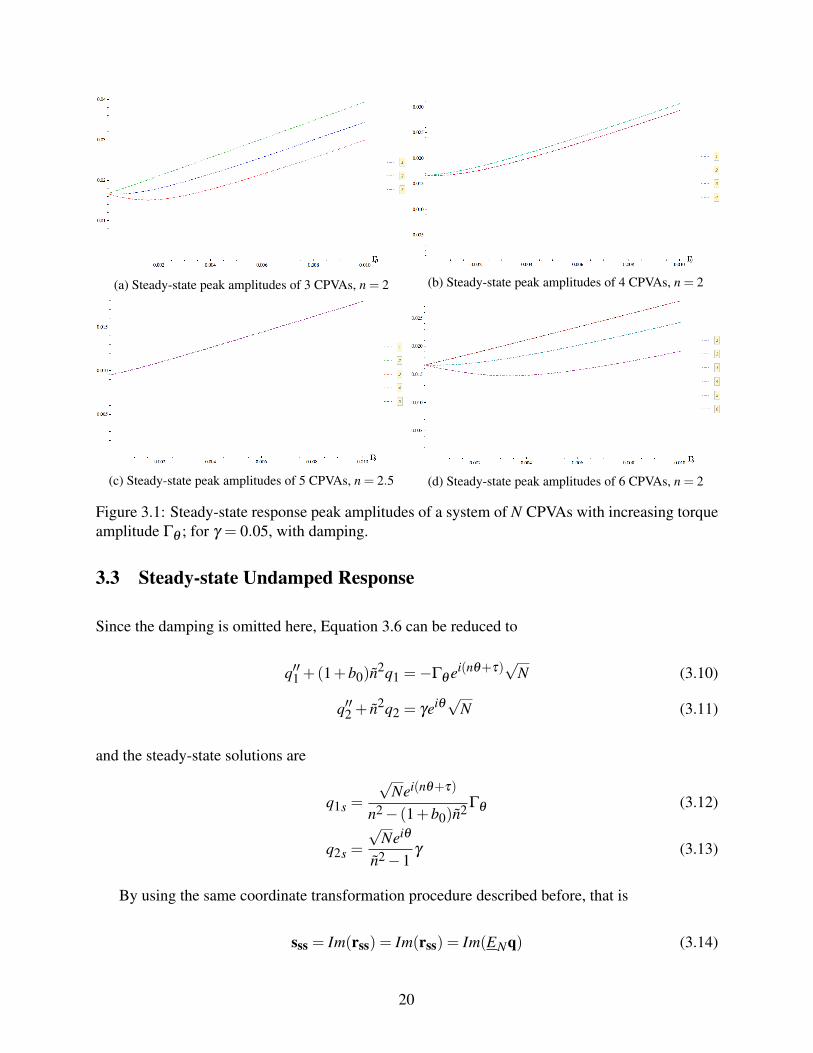
(a) Steady-state peak amplitudes of 3 CPVAs, n = 2 (b) Steady-state peak amplitudes of 4 CPVAs, n = 2

(c) Steady-state peak amplitudes of 5 CPVAs, n = 2.5 (d) Steady-state peak amplitudes of 6 CPVAs, n = 2

Figure 3.1: Steady-state response peak amplitudes of a system of N CPVAs with increasing torqueamplitude Γθ ; for γ = 0.05, with damping.

3.3 Steady-state Undamped Response

Since the damping is omitted here, Equation 3.6 can be reduced to

q′′1 +(1+b0)n2q1 =−Γθ ei(nθ+τ)

√N (3.10)

q′′2 + n2q2 = γeiθ√N (3.11)

and the steady-state solutions are

q1s =

√Nei(nθ+τ)

n2− (1+b0)n2 Γθ (3.12)

q2s =

√Neiθ

n2−1γ (3.13)

By using the same coordinate transformation procedure described before, that is

sss = Im(rss) = Im(rss) = Im(ENq) (3.14)

20

the steady-state response of the absorbers can be obtained as

ss =

√N

n2−(1+b0)n2 Γθ sin(nθ + τ)+

√N]

n2−1γ sin(θ)

√N

n2−(1+b0)n2 Γθ sin(nθ + τ)+

√N

n2−1γ sin(θ + 2π

N )

...

...

√N

n2−(1+b0)n2 Γθ sin(nθ + τ)+

√N

n2−1γ sin(θ + 2π

N (N−1))

(3.15)

Equation 3.15 shows that each absorber response has an order n response with a common

amplitude, and an order 1 response with a common amplitude. This is a key to the assumption of

the general CPVA response formulation in the grouping analysis in Section 2.3.

21

CHAPTER 4

ACCOUNTING FOR GRAVITATIONAL PARAMETRIC EXCITATION -PERTURBATION ANALYSIS

When the parametric excitation from gravity is kept in the model, the equations are linear with

time-periodic coefficients. While the steady-state responses can be expressed in terms of integrals,

a convenient way to obtain approximations of these is to employ perturbation methods; here we

use the method of multiple scales (MMS). To this end we need to introduce a small parameter

ε to be used in the expansions. For simplicity in development, we begin with an analysis of the

undamped system with one and then N absorbers, and then consider the effects of damping at the

end of the chapter.

4.1 Scaling

There are several terms in Equation 2.11 that are scaled by ε , namely

b0 = εB

δ , εP p,s′′ = εP p′′,ω ′ = ε

Wξ′,γ = ε

Gγ,Γθ = ε

ΓΓθ , n = n(1+ ε

Qσ). (4.1)

These are consistent with applications, as the parameters and variables above are assumed small.

Note that δ is a variable that is used to trace the inertia ratio b0 in the scaled equations, and it can

be taken to be unity so that εB becomes the inertia ratio.

4.2 Single Absorber Case

The perturbation analysis is based on the linearized, non-dimensional equation with the parametric

excitation term present. The simplest system to analyze is a single absorber attached to the rotor,

as the cyclic phase has no effect in this case. The equation is formulated as

s′′+(1+b0)(n2− (1+ n2)γ cos(θ))s =−Γθ sin(nθ + τ)+(1+b0)γ sin(θ) (4.2)

22

By using the scaling in Equation 4.1 in 4.2, the equation of motion becomes

εP p′′+n2(εP+B

δ + εP)p+2n2

σ(εQ+P+Bδ + ε

Q+P)p− (1+n2)γ cos(θ)(εG+B+Pδ + ε

G+P)p

−2n2σγ cos(θ)(εG+B+P+Q

δ + εG+P+Q)p =−ε

ΓΓθ sin(nθ + τ)+(εG + ε

G+Bδ )γ sin(θ)

(4.3)

In Equation 4.3, in order to keep the parametric term at leading order, along with the other effects

of interest, we choose G = 12 , B = 1

2 , Q = 12 , P = 1

2 , and Γ = 1. Thus, Equation 4.3, when expanded

to leading order in ε , becomes

p′′+n2 p+ε12 [n2

δ +2n2σ − (1+n2)γ cos(θ)]p

= ε12 (−Γθ sin(nθ + τ)+δ γ sin(θ))+ γ sin(θ)+HOT (4.4)

where HOT refers to higher order terms.

It is convenient to define ε12 = ε , so that Equation 4.4, with removal of the HOT, is given by

p′′+n2 p+ ε[n2δ +2n2

σ − (1+n2)γ cos(θ)]p = ε(−Γθ sin(nθ + τ)+δ γ sin(θ))+ γ sin(θ)

(4.5)

Note that, according to the terminology in [4], this is a case of hard non-resonant and weak

resonant excitation (assuming n 6= 1, which is consistent with cases of practical interest).

Following the standard procedure for the MMS, the absorber response can be expressed as an

expansion of p:

p = p0 + ε p1 + ...

where both p0 and p1 are depend on scales θ0 = θ and θ1 = εθ .

Gathering ε0 and ε1 terms separately provides the following two equations

ε0 : D2

0 p0 +n2 p0 = γ sin(θ0) (4.6)

ε1 : D2

0 p1 +n2 p1 =−2D0D1 p0− [n2δ +2n2

σ − (1+n2)γ cos(θ0)]p0 +δ γ sin(θ0)− Γθ sin(nθ0 + τ)

(4.7)

where D0 is the partial derivative respect to the rotor angle scale θ0 and D1 is the partial derivative

respect to the scale θ1.

23

From the ε0 equation, the solution for p0 is given by

p0 = Aeinθ0 +Λeiθ0 + c.c. (4.8)

where Λ = γ

2i(n2−1)and it is convenient to express A = 1

2aeiβ , which is a function of θ1.

Inserting Equation 4.8 into the ε1 equation in Equation 4.6 and expanding, we find the follow-

ing equation for p1:

ε1 :D0

2 p1 +n2 p1 =−2D0D1(Aeinθ0 +Λeiθ0 + c.c.) (4.9)

−n2δ (Aeinθ0 +Λeiθ0 + c.c.)−2n2

σ(Aeinθ0 +Λeiθ0 + c.c.) (4.10)

+12

γ(1+n2)(eiθ0 + e−iθ0)(Aeinθ0 +Λeiθ0 + c.c.)+12i

δ γ(eiθ0− e−iθ0) (4.11)

− 12i

Γθ (ei(nθ0+τ)− e−i(nθ0+τ)) (4.12)

It can be seen that in some cases there are some terms in Equation 4.9 leads to unbounded as

θ0 evolves. These terms are called secular terms, which can vary depending on the value of n.

According Equation 4.9, the possible cases are: n = 1, n = 2, and n 6= 1,2. In this chapter, cases

n = 2 and n 6= 1,2 are considered as, when n = 2, both torque gravity parameters contribute to

resonating order n response of abosorber. n = 1 case is recommended for future work.

For the case n = 2, the slow flow equation is obtained by equating the secular terms to zero. In

other words,

(−2inA′− (n2δ +2n2

σ)A+12

γ(1+n2)Λ− 12i

Γθ eiτ)einθ0 = 0 (4.13)

The following equations below are obtained by taking the real and imaginary parts of Equation

4.13:

Re : aβ′− (

12

δna+nσa)− 14n

(1+n2)γ2

(n2−1)sin(β )+

12n

Γθ sin(β − τ) = 0

Im : a′+1

4n(1+n2)γ2

(n2−1)cos(β )− 1

2nΓθ cos(β − τ) = 0 (4.14)

It is convenient to use ∆ = n2+14n(n2−1)

γ2, which contains the parametric effect, for all of the rest of

analysis. (Note: n is kept here just to show the general formulation).

24

In order to solve Equation set 4.14 for the steady-state solution, the terms a′ and β ′ are set to

zero, which indicates a constant phase and amplitude for A. From the imaginary part of Equation

4.14, if and only if τ = 0, the only value for β to make it valid is β = π2 . Thus, a is solved after

substituting β value into the real part of Equation 4.14

a =1

n2(δ +2σ)Γθ −

2∆

n(δ +2σ)(4.15)

For n 6= 1,2, the only difference from Equation 4.13 is that the term 12 γ(1+n2)Λ is excluded. So

the slow-flow equation in the form of imaginary and real parts are

Re : aβ′− (

12

δna+nσa)+1

2nΓθ sin(β − τ) = 0

Im : a′− 12n

Γθ cos(β − τ) = 0 (4.16)

and the steady-state solution for Equation 4.16 is

β =π

2

a =1

n2(δ +2σ)Γθ (4.17)

4.3 Multiple Absorbers Case

Using the same scaling method from Section 4.1 on the linearized equations for multiple CPVAs,

namely Equation 2.11, with an additional s j′′ = ε

12 p j′′, the following equation is obtained

(p′′j +n2 p j− γ sin(θ j))+ ε12 [(δ p′′j −

1N

N

∑k=1

p′′k )δ +(n2δ +2n2

σ − γ(1+n2)cos(θ j))p j

−δ γ sin(θ j)+ Γθ sin(nθ + τ)]+HOT = 0 (4.18)

where θ j = θ0+2π( j−1)

N and j = 1,2, ...,N. From the leading order part, p′′j +n2 p j− γ sin(θ j) =

0, it can be seen that the term p′′j is replaceable with −n2 p j + γ sin(θ j) in the summation. In

addition, the terms n2δ p j and δ γ sin(θ j) can also be canceled by the term δ p′′j . Those are the main

differences from the equation for the single absorber case. It is also convenient to use ε = ε12 .In

25

this case the equations at orders ε0 and ε1 are given by

ε0 : D2

0 p0 j +n2 p0 j = γ sin(θ j)

ε1 : D2

0 p1 j +n2 p1 j =−2D0D1 p0 j−1N

δn2N

∑k=1

p0k (4.19)

− [2n2σ − (1+n2)γ cos(θ j)]p0 j− Γθ sin(nθ0 + τ).

The solution of the ε0 equations are

p0 j = A jeinθ0 +Λei(θ j)+ c.c. (4.20)

where Λ = γ

2i(n2−1)and the A j are to be determined.

By replacing p0 j in the ε1 equation with the expression in Equation 4.20, the following equa-

tion is obtained for p1 j:

ε1 :D0

2 p1 j +n2 p1 j =−2D0D1(A jeinθ0 +Λei(θ0+φ j)+ c.c.)

− 1N

δn2N

∑k=1

(Akeinθ0 +Λei(θ0+φk)+ c.c.)−2n2σ(A je

inθ0 +Λei(θ0+φ j)+ c.c.)

+12

γ(1+n2)(ei(θ0+φ j)+ e−i(θ0+φ j))(A jeinθ0 +Λei(θ0+φ j)+ c.c.)− 1

2iΓθ (e

i(nθ0+τ)− e−i(nθ0+τ))

Just as mentioned in Section 4.2 for single absorber, n = 2 and n 6= 1,2 cases are considered,

because both gravity and torque are involved in order n response when n = 2, while for other value

(not 1) of n there is only torque.

For the case when n = 2, by gathering the secular terms and setting them equal to zero, we find

the following slow flow equation for the complex amplitudes A j:

2inA′j +2n2σA j +

12i

Γθ eiτ − 12

γ(1+n2)Λei2φ j +δn2

N

N

∑k=1

Ak = 0 (4.21)

For other cases where n 6= 2, by equating all the secular terms to zero, the following slow flow

equation is obtained:

2inA′j +2n2σA j +

12i

Γθ eiτ +δn2

N

N

∑k=1

Ak = 0 (4.22)

26

where A j is a function of θ1, and Λ = γ

2i(n2−1).

A convenient form for Equation 4.21 and Equation 4.22 is obtained by introducing A j =

12a je

iβ j and separating the real and imaginary parts, resulting in the following slow flow equa-

tions for the amplitude and phase

n = 2:

Re :−a jβ′j +nσa j−

Γθ

2nsin(β j− τ)−∆sin(2φ j−β j)+

δn2N

N

∑k=1

[ak cos(βk−β j)] = 0

Im : a′j−Γθ

2ncos(β j− τ)+∆cos(2φ j−β j)+

δn2N

N

∑k=1

[ak sin(βk−β j)] = 0 (4.23)

(Note: n is kept here so that a general formulation can be presented)

n 6= 1,2:

Re :−a jβ′j +nσa j−

Γθ

2nsin(β j− τ)+

δn2N

N

∑k=1

[ak cos(βk−β j)] = 0

Im : a′j−Γθ

2ncos(β j− τ)+

δn2N

N

∑k=1

[ak sin(βk−β j)] = 0 (4.24)

From Equation 4.23 and 4.24, it is seen that the phases of the absorbers are coupled, which

makes it hard to solve for a j and β j. However, since it is linear, it is convenient to express the A j

in terms of Cartesian coordinates.

4.4 Slow Flow in Cartesian Coordinates

The form A j =12a je

iβ j is a common expression in polar coordinate in real-imaginary coordinates.

It can also be expressed in Cartesian coordinates, as in the form of

A j =12(u j + iv j) (4.25)

where u j = a j cos(β j), and v j = a j sin(β j). Thus, the amplitude a j can be expressed by√u j2 + v j2, and the phase β = arctan(

v ju j) .

27

By substituting the form of 4.25 into Equation 4.21 for n = 2 case and Equation 4.22, n = 2:

Im : u j′ =− δn

2N

N

∑k=1

vk−nσv j−∆cos(2φ j)+1

2nΓθ cos(τ)

Re : v j′ =

δn2N

N

∑k=1

uk +nσu j−∆sin(2φ j)+12n

Γθ sin(τ) (4.26)

n 6= 1,2:

Im : u j′ =− δn

2N

N

∑k=1

vk−nσv j +1

2nΓθ cos(τ)

Re : v j′ =

δn2N

N

∑k=1

uk +nσu j +1

2nΓθ sin(τ) (4.27)

It can be seen that equations 4.26 and 4.27 are both linear in v j and u j and therefore solvable

in a quite straightforward manner.

The steady-state solutions are found by setting u j′ and v j

′ equal to zero. The resulting versions

of Equations 4.26 and 4.27 can be expressed in a matrix form as

Az = F (4.28)

where A is the (2N×2N) coefficient matrix, which is also a block-circulant [7] of N 2×2 matrices,

in the form of

A =

J L . . . L

L J . . . L

...... . . . ...

L L . . . J

where J and L are

J =

nσ + n

2N δ 0

0 nσ + n2N δ

, L =

n

2N δ 0

0 n2N δ

28

and z = [u1,v1,u2,v2, . . . ,uN ,vN ]T . The A matrix is the same for all n.

For other n 6= 1,2, the force vector contains only the applied torque and is given by

F = FT =1

2nΓθ

−sin(τ)

cos(τ)

...

−sin(τ)

cos(τ)

For n = 2 the force vector is a combination of the applied torque and the gravitational paramet-

ric excitation force, in the form

F = FT +FG =1

2nΓθ

−sin(τ)

cos(τ)

...

−sin(τ)

cos(τ)

+∆

sin(2φ1)

−cos(2φ1)

...

sin(2φN)

−cos(2φN)

which shows why the n = 2 case stands out.

It is clear to see that matrix A is a circulant matrix, which, by introducing Fourier matrix, can

be diagonalized, as seen in Section 3.2. In this way, the solutions for z can be easily solved in

closed form, as follows. The diagnoalized version of A is represented by A = E†2NAE2N , which

is a block matrix with two D (N×N) arranged diagonally, given by

A =

D 0N×N

0N×N D

29

where

D =

nσ + n2δ 0 0 . . . 0

0 nσ 0 . . . 0

0 0 nσ . . . 0

0 0 0 . . . 0

0 0 0 . . . nσ

Since the torque excitation part in the force vector F is the same for all n 6= 1, then the trans-

formed form is also the same, which can be treated as two N× 1, FT1 and FT2, vectors joined

together,

FT = E†NFT =

√N

2nΓθ

FT1

FT2

where

FT1 =

−sin(τ)+ cos(τ)

0

...

0

, FT2 =

−sin(τ)− cos(τ)

0

...

0

When n= 2, the phases in the gravity part in the force vector, FG makes the transformation pro-

cedure more complicated and the transformed expression, FG, varies with the number of absorber,

N. Thus, the form FG will not be presented.

The problem with these undamped cases is that, when the absorbers are perfect tuned, σ = 0,

the coefficient matrix, either the original or diagonalized, becomes singular. This makes the system

unsolvable. Thus, for the perfectly tuned absorber cases, it is necessary to add damping.

30

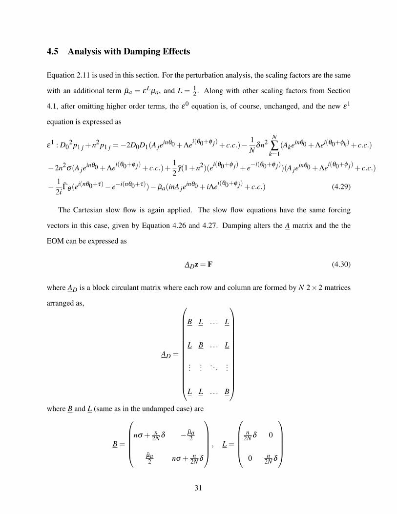
4.5 Analysis with Damping Effects

Equation 2.11 is used in this section. For the perturbation analysis, the scaling factors are the same

with an additional term µa = εLµa, and L = 12 . Along with other scaling factors from Section

4.1, after omitting higher order terms, the ε0 equation is, of course, unchanged, and the new ε1

equation is expressed as

ε1 : D0

2 p1 j +n2 p1 j =−2D0D1(A jeinθ0 +Λei(θ0+φ j)+ c.c.)− 1

Nδn2

N

∑k=1

(Akeinθ0 +Λei(θ0+φk)+ c.c.)

−2n2σ(A je

inθ0 +Λei(θ0+φ j)+ c.c.)+12

γ(1+n2)(ei(θ0+φ j)+ e−i(θ0+φ j))(A jeinθ0 +Λei(θ0+φ j)+ c.c.)

− 12i

Γθ (ei(nθ0+τ)− e−i(nθ0+τ))− µa(inA je

inθ0 + iΛei(θ0+φ j)+ c.c.) (4.29)

The Cartesian slow flow is again applied. The slow flow equations have the same forcing

vectors in this case, given by Equation 4.26 and 4.27. Damping alters the A matrix and the the

EOM can be expressed as

ADz = F (4.30)

where AD is a block circulant matrix where each row and column are formed by N 2×2 matrices

arranged as,

AD =

B L . . . L

L B . . . L

...... . . . ...

L L . . . B

where B and L (same as in the undamped case) are

B =

nσ + n

2N δ − µa2

µa2 nσ + n

2N δ

, L =

n

2N δ 0

0 n2N δ

31

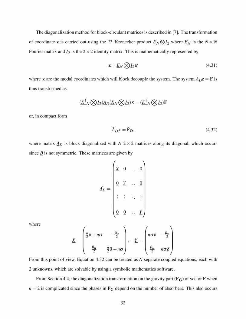
The diagonalization method for block-circulant matrices is described in [7]. The transformation

of coordinate z is carried out using the ?? Kronecker product EN⊗

I2 where EN is the N ×N

Fourier matrix and I2 is the 2×2 identity matrix. This is mathematically represented by

z = EN⊗

I2κ (4.31)

where κ are the modal coordinates which will block decouple the system. The system ADz = F is

thus transformed as

(E†N⊗

I2)AD(EN⊗

I2)κ = (E†N⊗

I2)F

or, in compact form

ADκ = FD. (4.32)

where matrix AD is block diagonalized with N 2× 2 matrices along its diagonal, which occurs

since B is not symmetric. These matrices are given by

AD =

X 0 . . . 0

0 Y . . . 0

...... . . . ...

0 0 . . . Y

where

X =

n2δ +nσ − µa

2

µa2

n2δ +nσ

, Y =

nσδ − µa

2

µa2 nσδ

From this point of view, Equation 4.32 can be treated as N separate coupled equations, each with

2 unknowns, which are solvable by using a symbolic mathematics software.

From Section 4.4, the diagonalization transformation on the gravity part (FG) of vector F when

n = 2 is complicated since the phases in FG depend on the number of absorbers. This also occurs

32

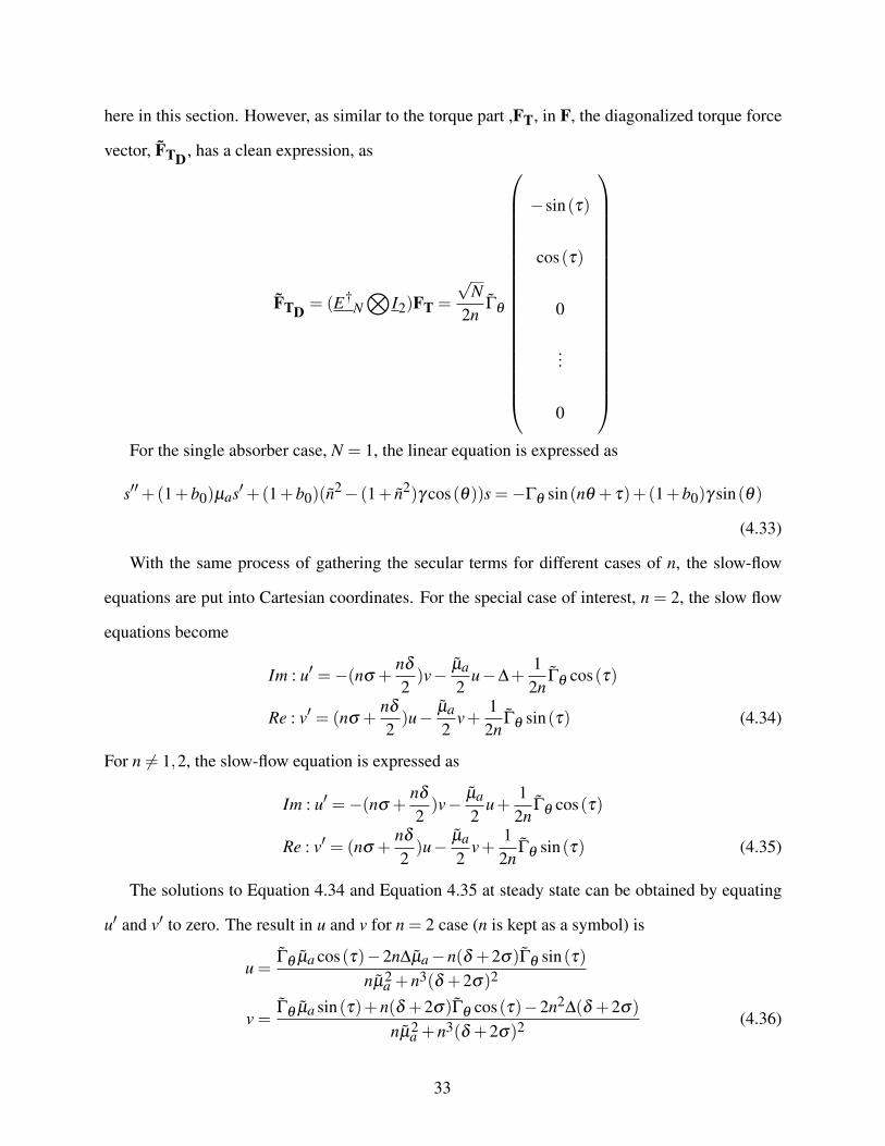
here in this section. However, as similar to the torque part ,FT, in F, the diagonalized torque force

vector, FTD , has a clean expression, as

FTD = (E†N⊗

I2)FT =

√N

2nΓθ

−sin(τ)

cos(τ)

0

...

0

For the single absorber case, N = 1, the linear equation is expressed as

s′′+(1+b0)µas′+(1+b0)(n2− (1+ n2)γ cos(θ))s =−Γθ sin(nθ + τ)+(1+b0)γ sin(θ)

(4.33)

With the same process of gathering the secular terms for different cases of n, the slow-flow

equations are put into Cartesian coordinates. For the special case of interest, n = 2, the slow flow

equations become

Im : u′ =−(nσ +nδ

2)v− µa

2u−∆+

12n

Γθ cos(τ)

Re : v′ = (nσ +nδ

2)u− µa

2v+

12n

Γθ sin(τ) (4.34)

For n 6= 1,2, the slow-flow equation is expressed as

Im : u′ =−(nσ +nδ

2)v− µa

2u+

12n

Γθ cos(τ)

Re : v′ = (nσ +nδ

2)u− µa

2v+

12n

Γθ sin(τ) (4.35)

The solutions to Equation 4.34 and Equation 4.35 at steady state can be obtained by equating

u′ and v′ to zero. The result in u and v for n = 2 case (n is kept as a symbol) is

u =Γθ µa cos(τ)−2n∆µa−n(δ +2σ)Γθ sin(τ)

nµ2a +n3(δ +2σ)2

v =Γθ µa sin(τ)+n(δ +2σ)Γθ cos(τ)−2n2∆(δ +2σ)

nµ2a +n3(δ +2σ)2 (4.36)

33

Then order n response amplitude is obtained as

a =

√Γ2

θ+4n2∆2−4nΓθ ∆cos(τ)

n2(µ2a +n2(δ +2σ)2)

(4.37)

and when τ = 0, a can be rewritten as

a =

√(Γθ −2n∆)2

n2(µ2a +n2(δ +2σ)2)

(4.38)

It can be seen that, when τ = 0, if the non-dimensional gravity term, γ , is constant, then there will

be a critical value for Γθ that will kill order n (in this case, n = 2) response.

For n 6= 1,2, the solutions for u and v have the same denominator, and there is no ∆, such that

u =Γθ µa cos(τ)−n(δ +2σ)Γθ sin(τ)

nµ2a +n3(δ +2σ)2

v =Γθ µa sin(τ)+n(δ +2σ)Γθ cos(τ)

nµ2a +n3(δ +2σ)2 (4.39)

and the order n amplitude is expressed as

a =Γθ

n√(µ2

a +n2(δ +2σ)2)(4.40)

For the multiple absorber cases, the transformation from coordinates κ back to z is very messy.

Thus, the expressions are not presented in this paper.

We present results from this analysis after considering how these absorber responses affect the

dynamics of the rotor, which is the ultimate motivation for using CPVAs.

4.6 Rotor Behavior Analysis

The overall goal for CPVAs is to reduce torsional vibrations on the rotor, so in this section the

rotor perturbation equation is formulated. The rotor analysis is based on the solutions from the

absorbers’ perturbation analysis. By substituting scaling factors and their values from Equation

4.1 into Equation 2.8, the rotor equations can be expressed as

εW

ξ′+

1N

ε1

∑j=1

N p j′′+HOT = ε

1Γθ sin(nθ + τ)

34

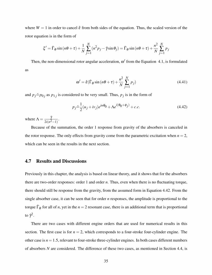
where W = 1 in order to cancel ε from both sides of the equation. Thus, the scaled version of the

rotor equation is in the form of

ξ′ = Γθ sin(nθ + τ)+

1N

N

∑j=1

(n2 p j− γ sinθ j) = Γθ sin(nθ + τ)+n2

N

N

∑j=1

p j

Then, the non-dimensional rotor angular acceleration, ω ′ from the Equation 4.1, is formulated

as

ω′ = ε(Γθ sin(nθ + τ)+

n2

N

N

∑j=1

p j) (4.41)

and p j=p0 j as p1 j is considered to be very small. Thus, p j is in the form of

p j=12(u j + iv j)e

inθ0 +Λei(θ0+φ j)+ c.c. (4.42)

where Λ = γ

2i(n2−1).

Because of the summation, the order 1 response from gravity of the absorbers is canceled in

the rotor response. The only effects from gravity come from the parametric excitation when n = 2,

which can be seen in the results in the next section.

4.7 Results and Discussions

Previously in this chapter, the analysis is based on linear theory, and it shows that for the absorbers

there are two-order responses: order 1 and order n. Thus, even when there is no fluctuating torque,

there should still be response from the gravity, from the assumed form in Equation 4.42. From the

single absorber case, it can be seen that for order n responses, the amplitude is proportional to the

torque Γθ for all of n, yet in the n = 2 resonant case, there is an additional term that is proportional

to γ2.

There are two cases with different engine orders that are used for numerical results in this

section. The first case is for n = 2, which corresponds to a four-stroke four-cylinder engine. The

other case is n= 1.5, relevant to four-stroke three-cylinder engines. In both cases different numbers

of absorbers N are considered. The difference of these two cases, as mentioned in Section 4.4, is

35

the appearance of the parametric term when n= 2. In fact, these parametric resonance terms appear

only when n = 1,2, and n = 1 is not of much practical interest, so we select n = 2 to demonstrate

the effects of parametric resonance.

The simplest system that demonstrates the effects of the parametric effects on the absorbers

from gravity is that with a single absorber, N = 1. The numerical simulation of Equation 2.11 with

a single CPVA is conducted in MATLAB with parameters δ = 1, ε = 0.0355 , γ = 0.05, τ = 0

and Γθ in the range from 0 to 0.01, at a mean speed of 400 rpm, the damping ratio is set to be

ζ = 0.01, so that µa varies with different values of n. For n = 2 the damping coefficient µa = 0.04

and for n = 1.5, µa = 0.03. In order to see the relationship between the absorber response and

the amplitude of the fluctuating torque, the peak amplitude of the absorber response at each torque

level is plotted.

Figure 4.1: Steady-state response amplitudes of a single (N = 1) CPVA with increasing torque,Γθ ; for γ = 0.05, n = 2, µa = 0.04, and σ = 0.

The results from analysis and simulation match well, as can be seen in the plots shown below.

In Figure 4.1, with the amplitude of the fluctuating torque increasing, the absorber amplitude goes

down at first and then increases, which is caused by order n response in this case, supported by

36

Equation 4.38. This behavior comes from the parametric excitation effects from gravity. A time-

trace plot of this case n = 2 is provided in Figure 4.2b at the critic torque (Γθ2 from Figure 4.1).

It clearly shows that the absorbers have only one harmonic response. Figure 4.2 also shows the

(a) At Γθ1(b) At Γθ2

(c) At Γθ3

Figure 4.2: Steady-state response amplitudes of a single (N = 1) CPVA time-trace plot at varioustorque level, for γ = 0.05, n = 2, µa = 0.04, and σ = 0.

transition of absorber behaviors from less torque levels (Γθ1 from Figure 4.1) to the higher torque

levels (Γθ3 from Figure 4.1).

Figure 4.3 shows the absorber response for n = 1.5, in which case parametric term is not reso-

nant and the absorber amplitude grows linearly at the torque increases. An interesting observation

from these two figures is that when there is no fluctuating torque, Γθ = 0, the absorber has a

non-zero response due to the direct excitation from gravity, with amplitude given by Equation 4.8.

From the solution expressions of order n amplitudes for the undamped case, Equation 4.15 and

Equation 4.17, it is clear to see the difference from the ones of the damped cases, specifically in

Equation 4.37 and Equation 4.40. Then it is more visual to see the effects of the damping in graphic

forms. The results of the undamped response and those with damping of ζ = 0.01 are plotted in

Figure 4.4 and Figure 4.5 for n = 2 and n = 1.5, respectively.

In Figure 4.4, it is clearly shown that the "dip" occurs with or without damping. Also, when the

torque amplitude is small, the damping does not have much influence on the absorber amplitude.

However, as the torque increases, the damped and undamped response amplitudes start to differ.

This separation also occurs in the n = 1.5 case, as shown in Figure 4.5. In addition, as expected,

the response amplitudes at moderate and large torques are smaller in the damped cases.

37

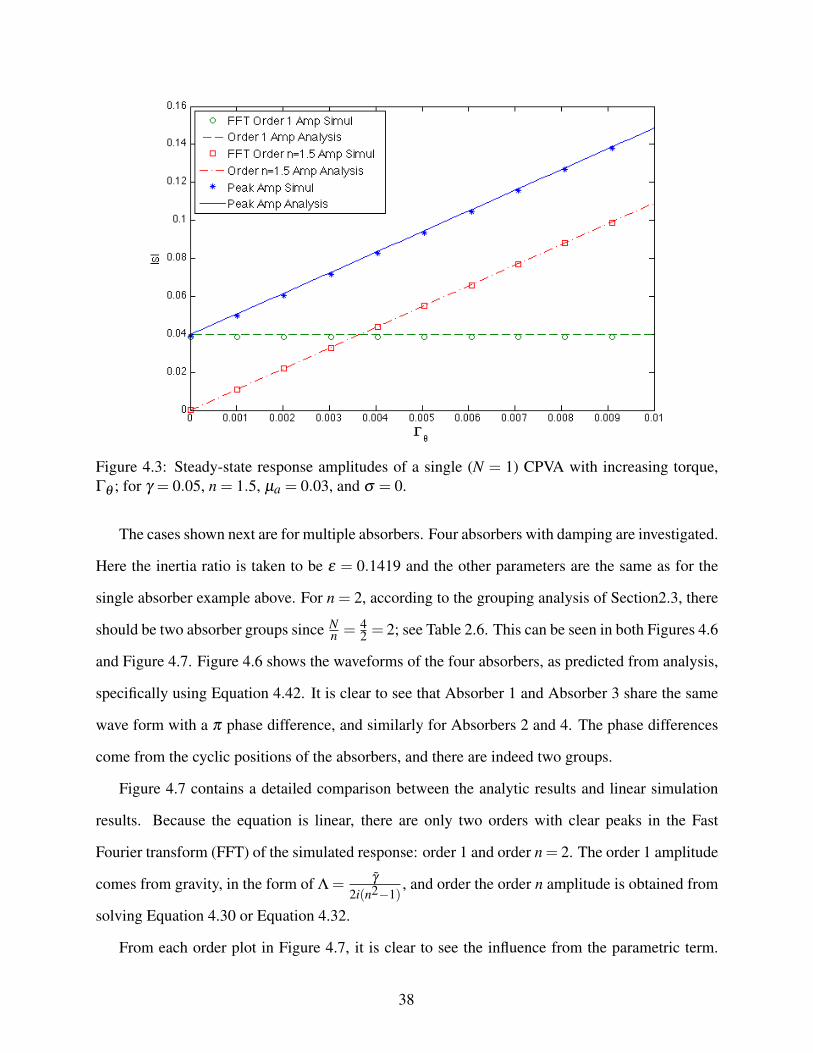
Figure 4.3: Steady-state response amplitudes of a single (N = 1) CPVA with increasing torque,Γθ ; for γ = 0.05, n = 1.5, µa = 0.03, and σ = 0.

The cases shown next are for multiple absorbers. Four absorbers with damping are investigated.

Here the inertia ratio is taken to be ε = 0.1419 and the other parameters are the same as for the

single absorber example above. For n = 2, according to the grouping analysis of Section2.3, there

should be two absorber groups since Nn = 4

2 = 2; see Table 2.6. This can be seen in both Figures 4.6

and Figure 4.7. Figure 4.6 shows the waveforms of the four absorbers, as predicted from analysis,

specifically using Equation 4.42. It is clear to see that Absorber 1 and Absorber 3 share the same

wave form with a π phase difference, and similarly for Absorbers 2 and 4. The phase differences

come from the cyclic positions of the absorbers, and there are indeed two groups.

Figure 4.7 contains a detailed comparison between the analytic results and linear simulation

results. Because the equation is linear, there are only two orders with clear peaks in the Fast

Fourier transform (FFT) of the simulated response: order 1 and order n = 2. The order 1 amplitude

comes from gravity, in the form of Λ = γ

2i(n2−1), and order the order n amplitude is obtained from

solving Equation 4.30 or Equation 4.32.

From each order plot in Figure 4.7, it is clear to see the influence from the parametric term.

38

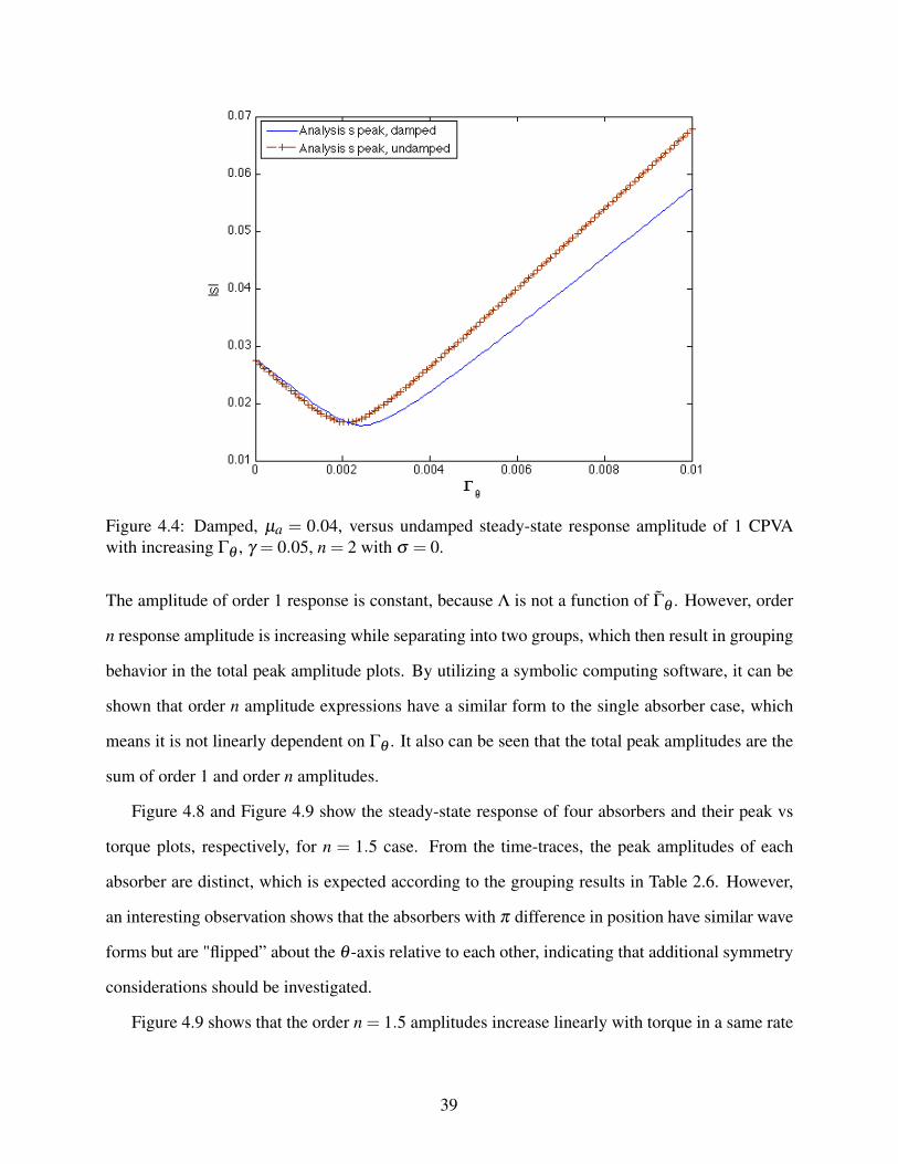
Figure 4.4: Damped, µa = 0.04, versus undamped steady-state response amplitude of 1 CPVAwith increasing Γθ , γ = 0.05, n = 2 with σ = 0.

The amplitude of order 1 response is constant, because Λ is not a function of Γθ . However, order

n response amplitude is increasing while separating into two groups, which then result in grouping

behavior in the total peak amplitude plots. By utilizing a symbolic computing software, it can be

shown that order n amplitude expressions have a similar form to the single absorber case, which

means it is not linearly dependent on Γθ . It also can be seen that the total peak amplitudes are the

sum of order 1 and order n amplitudes.

Figure 4.8 and Figure 4.9 show the steady-state response of four absorbers and their peak vs

torque plots, respectively, for n = 1.5 case. From the time-traces, the peak amplitudes of each

absorber are distinct, which is expected according to the grouping results in Table 2.6. However,

an interesting observation shows that the absorbers with π difference in position have similar wave

forms but are "flipped” about the θ -axis relative to each other, indicating that additional symmetry

considerations should be investigated.

Figure 4.9 shows that the order n = 1.5 amplitudes increase linearly with torque in a same rate

39

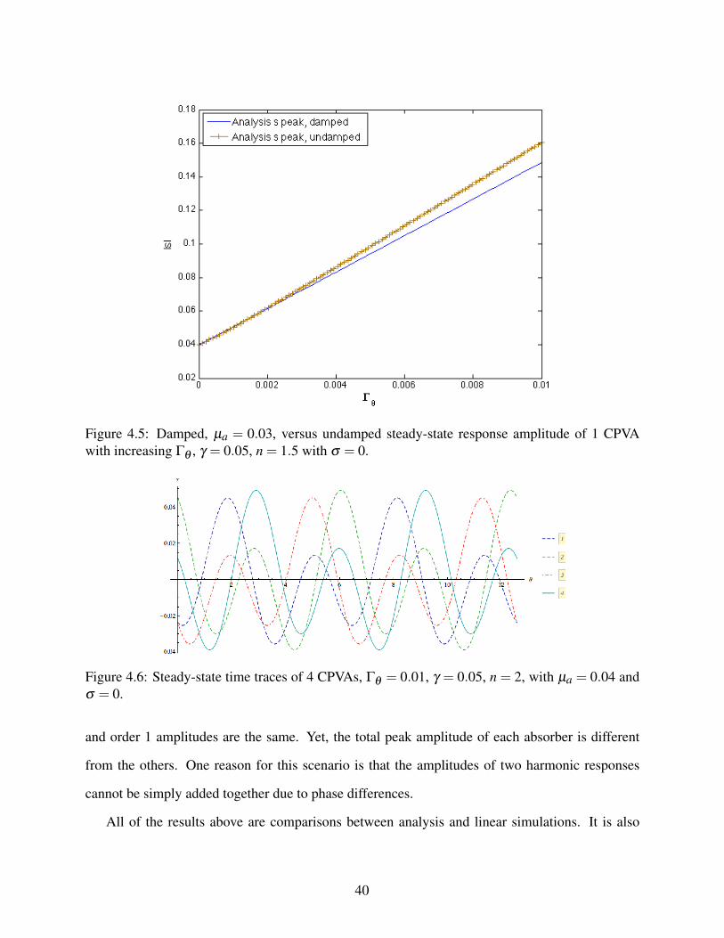
Figure 4.5: Damped, µa = 0.03, versus undamped steady-state response amplitude of 1 CPVAwith increasing Γθ , γ = 0.05, n = 1.5 with σ = 0.

Figure 4.6: Steady-state time traces of 4 CPVAs, Γθ = 0.01, γ = 0.05, n = 2, with µa = 0.04 andσ = 0.

and order 1 amplitudes are the same. Yet, the total peak amplitude of each absorber is different

from the others. One reason for this scenario is that the amplitudes of two harmonic responses

cannot be simply added together due to phase differences.

All of the results above are comparisons between analysis and linear simulations. It is also

40

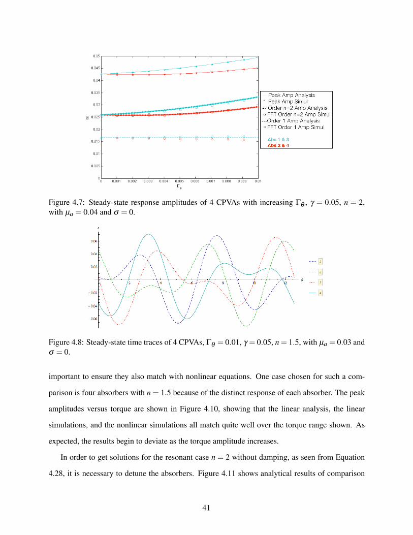
Figure 4.7: Steady-state response amplitudes of 4 CPVAs with increasing Γθ , γ = 0.05, n = 2,with µa = 0.04 and σ = 0.

Figure 4.8: Steady-state time traces of 4 CPVAs, Γθ = 0.01, γ = 0.05, n = 1.5, with µa = 0.03 andσ = 0.

important to ensure they also match with nonlinear equations. One case chosen for such a com-

parison is four absorbers with n = 1.5 because of the distinct response of each absorber. The peak

amplitudes versus torque are shown in Figure 4.10, showing that the linear analysis, the linear

simulations, and the nonlinear simulations all match quite well over the torque range shown. As

expected, the results begin to deviate as the torque amplitude increases.

In order to get solutions for the resonant case n = 2 without damping, as seen from Equation

4.28, it is necessary to detune the absorbers. Figure 4.11 shows analytical results of comparison

41

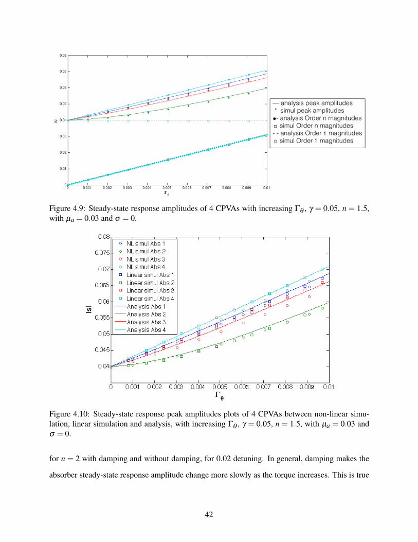
Figure 4.9: Steady-state response amplitudes of 4 CPVAs with increasing Γθ , γ = 0.05, n = 1.5,with µa = 0.03 and σ = 0.

Figure 4.10: Steady-state response peak amplitudes plots of 4 CPVAs between non-linear simu-lation, linear simulation and analysis, with increasing Γθ , γ = 0.05, n = 1.5, with µa = 0.03 andσ = 0.

for n = 2 with damping and without damping, for 0.02 detuning. In general, damping makes the

absorber steady-state response amplitude change more slowly as the torque increases. This is true

42

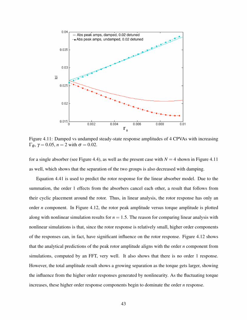
Figure 4.11: Damped vs undamped steady-state response amplitudes of 4 CPVAs with increasingΓθ , γ = 0.05, n = 2 with σ = 0.02.

for a single absorber (see Figure 4.4), as well as the present case with N = 4 shown in Figure 4.11

as well, which shows that the separation of the two groups is also decreased with damping.

Equation 4.41 is used to predict the rotor response for the linear absorber model. Due to the

summation, the order 1 effects from the absorbers cancel each other, a result that follows from

their cyclic placement around the rotor. Thus, in linear analysis, the rotor response has only an

order n component. In Figure 4.12, the rotor peak amplitude versus torque amplitude is plotted

along with nonlinear simulation results for n = 1.5. The reason for comparing linear analysis with

nonlinear simulations is that, since the rotor response is relatively small, higher order components

of the responses can, in fact, have significant influence on the rotor response. Figure 4.12 shows

that the analytical predictions of the peak rotor amplitude aligns with the order n component from

simulations, computed by an FFT, very well. It also shows that there is no order 1 response.

However, the total amplitude result shows a growing separation as the torque gets larger, showing

the influence from the higher order responses generated by nonlinearity. As the fluctuating torque

increases, these higher order response components begin to dominate the order n response.

43

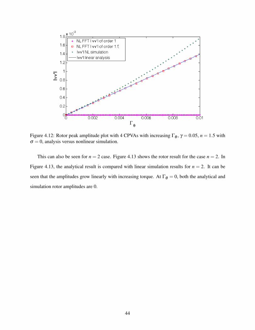
Figure 4.12: Rotor peak amplitude plot with 4 CPVAs with increasing Γθ , γ = 0.05, n = 1.5 withσ = 0, analysis versus nonlinear simulation.

This can also be seen for n = 2 case. Figure 4.13 shows the rotor result for the case n = 2. In

Figure 4.13, the analytical result is compared with linear simulation results for n = 2. It can be

seen that the amplitudes grow linearly with increasing torque. At Γθ = 0, both the analytical and

simulation rotor amplitudes are 0.

44

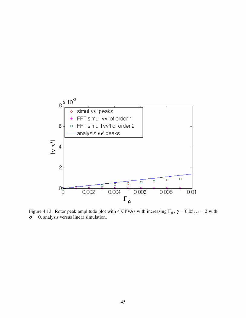
Figure 4.13: Rotor peak amplitude plot with 4 CPVAs with increasing Γθ , γ = 0.05, n = 2 withσ = 0, analysis versus linear simulation.

45

CHAPTER 5

CONCLUSIONS AND FUTURE WORK

5.1 Summary and Conclusions

The purpose of this work was to continue the investigation of the effects of gravity on rotor sys-

tems fitted with centrifugal pendulum vibration absorbers (CPVAs), as initiated by Theisen [10].

The main goals of the work were: (i) to investigate the specific effects of graviational parametric

excitation on the system, (ii) to exploit the cyclic nature of the gravitational excitation, and (iii) to

analyze the grouping behavior of absorbers for a given number of CPVAs, N and engine order, n.

These were done using a linearized mathematical model and numerical simulations.

A brief background of torsional vibrations and CPVAs was provided first. The equations of

motion for an idealized model were derived, linearized, and non-dimensionalized, which forms the

basis for the analysis. A general form of the absorber response at orders 1 and n was used to analyze

the grouping behavior of the absorbers. The grouping analysis was conducted by adding a dummy

phase variable into a general form of the jth absorber’s steady-state response and comparing that

with the ith absorber’s steady-state equation, to determine the conditions under which these two

absorbers would have identical waveforms. The answer to whether absorbers would behave in

groups was determined by whether Nn and n are integers, as summarized in Table 2.6. The results

from simulations showed that damping made the grouping more distinct, at least for some cases.

In the analysis, both resonant (n = 2) and non-resonant (n = 1.5) cases of practical interest

were studied. Models with and without parametric excitation, and with and without damping,

were considered. Expressions for the steady-state solutions for the absorbers were obtained and the

results showed that, without the parametric excitation term, solution of the system model could be

reduced to the diagonalization of a circulant matrix. This was achieved using the Fourier matrix [7]

to transform the system, and the transformed version of the excitation forces showed that gravity

46

excited only a single mode (an order one traveling wave mode) and the torque excited only another

single mode (the unison mode). This approach allows for an exact solution of the EOM in this

case.

For the linear steady-state response with parametric excitation, the equations were rescaled

so that a multiple time scales perturbation method was able to be conducted. A set of Cartesian

coordinates (u and v) was used for the order n amplitudes and phases instead of traditional polar

coordinates, since it transformed the slow-flow equations into linear functions of u and v. It was

shown that the order 1 amplitudes (from direct excitation from gravity) for all cases were constant

for a given mean rotor speed, as expected. For the steady-state solutions of the order n amplitudes,

it showed that the coefficient matrices were block-circulant, and the parametric term from gravity

only appeared in resonant n = 2 case. One note from the analysis was that when damping was

considered, the coefficient matrix could not be fully diagonalized, however, there were N sets

of two-by-two linear equations that could be solved in closed form. The analytic results were

compared with numerical simulations of both the linear and nonlinear model equations, showing

that the analytical predictions are accurate for small absorber amplitudes. A single-absorber case

was studied first in order to understand the effects of gravity for resonant, n = 2, and non-resonant,

n = 1.5, cases. In the non-resonant case (n = 1.5) it was seen that the absorber amplitude grows

linearly with increasing torque, as the order n response was not affected by the gravity. For the

resonant case (n = 2) the results show that, for a given value of γ , there was a critical torque

level where the parametric excitation from the gravity cancels the fluctuating torque, which left

only the order 1 response from the gravity at that point. For the case of multiple absorbers, the

results show that for both resonant and non-resonant cases, the order 1 component of the response

had a common amplitude for all absorbers. For n = 2, the order n response amplitude grows non-

linearly with the torque, due to the resonant interaction, and there was no scenario when the gravity

canceled the torque, as was the case with a single absorber. For n = 1.5, the results show that the

order n component of the absorbers’ responses have the same amplitude which grows linearly

with torque, similar to the single absorber case. However, because of the phase differences, the

47

peak amplitudes of the combined harmonics for each absorber can be different. From comparisons

between the damped and undamped cases, it was observed that damping does not change the

grouping behavior, but does affect the response of the absorbers in the expected manner, reducing

response amplitudes.

The response of the rotor was reconstructed using Equation 4.41 and the steady-state absorber

response. It was shown that, for multiple absorber systems, the effects of the order 1 responses on

the rotor cancel each other out in a summation, due to the cyclic nature of the order 1 response.

Thus, the rotor response includes only the order n absorber responses. It was also shown, using

simulations of the nonlinear equations, that nonlinear effects come into play at moderate ampli-

tudes, resulting in higher order harmonics in the rotor response, which are important since the

order n component is largely eliminated by the absorbers; this is consistent with previous observa-

tions [11].

5.2 Recommendations for Future Work

Information from the results of this study offer opportunities to examine other topics beyond the

conclusions of the study. These include:

• The effects of gravity on multiple absorber systems with general order torques, including the

resonant case n = 1.

• Analysis of nonlinear system models with gravity and near-tautochronic absorber paths.

• Analysis of models in which the inertia ratio is not small.

• Re-examination of the grouping behavior and analysis of higher order harmonics in the re-

sponse in light of nonlinear effects. As an example, it is noted from Figure 5.1 that the rotor

amplitude peak, from simulations of the nonlinear EOM, has a non-zero value when the or-

der n torque is zero. It is clear from the plot that this non-zero response comes from an order

48

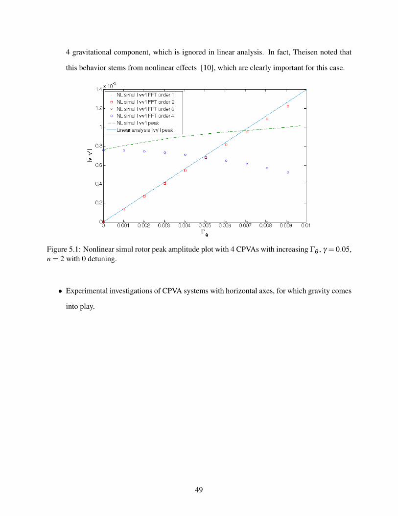
4 gravitational component, which is ignored in linear analysis. In fact, Theisen noted that

this behavior stems from nonlinear effects [10], which are clearly important for this case.

Figure 5.1: Nonlinear simul rotor peak amplitude plot with 4 CPVAs with increasing Γθ , γ = 0.05,n = 2 with 0 detuning.

• Experimental investigations of CPVA systems with horizontal axes, for which gravity comes

into play.

49

BIBLIOGRAPHY

50

BIBLIOGRAPHY

[1] Lindsay Brooke. “Chrysler sees the ICE future”. In: Automotive Engineering International20.S2 (2013), pp. 16–19.

[2] HH Denman. “Tautochronic bifilar pendulum torsion absorbers for reciprocating engines”.In: Journal of Sound and Vibration 159.2 (1992), pp. 251–277.

[3] J.F. Madden. Constant frequency bifilar vibration absorber. US Patent 4,218,187. 1980.URL: http://www.google.com/patents/US4218187.

[4] A.H. Nayfeh and D.T. Mook. Nonlinear Oscillations. Wiley Classics Library. Wiley, 2008.ISBN: 9783527617593. URL: https://books.google.com/books?id=sj3ebg7jRaoC.

[5] Tyler M Nester et al. Vibration reduction in a variable displacement engine using pendulumabsorbers. Tech. rep. SAE Technical Paper, 2003.

[6] David Edward Newland. “Nonlinear aspects of the performance of centrifugal pendulumvibration absorbers”. In: Journal of Manufacturing Science and Engineering 86.3 (1964),pp. 257–263.

[7] Brian J Olson et al. “Circulant matrices and their application to vibration analysis”. In:Applied Mechanics Reviews 66.4 (2014), p. 040803.

[8] Michael Swank and Patrick Lindemann. Dynamic absorbers for modern powertrains. Tech.rep. SAE Technical Paper, 2011.

[9] C.F. Taylor. The Internal-combustion Engine in Theory and Practice: Combustion, fuels,materials, design. The Internal-combustion Engine in Theory and Practice. M.I.T. Press,1985. ISBN: 9780262700276.

[10] T. Theisen. “Gravity’s Effect on Centrifugal Pendulum Vibration Absorbers”. M.S. Thesis.Michigan State University, 2011.

[11] Brendan J Vidmar et al. “Analysis and design of multiple order centrifugal pendulum vibra-tion absorbers”. In: ASME 2012 International Design Engineering Technical Conferencesand Computers and Information in Engineering Conference. American Society of Mechan-ical Engineers. 2012, pp. 165–173.

[12] W.K. Wilson. Practical solution of torsional vibration problems with examples from marineelectrical aeronautical and automobile engineering practice. Practical Solution of TorsionalVibration Problems With Examples from Marine Electrical Aeronautical and AutomobileEngineering Practice v. 3. Wiley, 1965. URL: https://books.google.com/books?id=9IYpAQAAMAAJ.

51