arX

iv:1

407.

3744

v3 [

mat

h.Q

A]

3 A

pr 2

015

digraphs.tex 2015-04-03 22:16 [1/40]

Graphs, hypergraphs, and properads

JOACHIM KOCK 1

kock@mat.uab.cat

Abstract

A categorical formalism for directed graphs is introduced, featuring naturalnotions of morphisms and subgraphs, and leading to two elementary descriptionsof the free-properad monad, first in terms of presheaves on elementary graphs,second in terms of groupoid-enriched hypergraphs.

Contents

Introduction 1

1 Graphs 31.1 Graphs . . . . . . . . . . . . . . . . . . . . . . . . . . . . . . . . . 31.2 Connectedness and acyclicity . . . . . . . . . . . . . . . . . . . . 61.3 Closed-graph adjunction . . . . . . . . . . . . . . . . . . . . . . . 71.4 Canonical neighbourhoods, covers and hulls . . . . . . . . . . . 81.5 Pushouts, coequalisers, and colimits over graphs . . . . . . . . . 101.6 Complements and convexity . . . . . . . . . . . . . . . . . . . . 13

2 Properads 152.1 Digraphical species (coloured bi-collections) and F-graphs . . . 162.2 The free-properad monad . . . . . . . . . . . . . . . . . . . . . . 172.3 Generic/free factorisation and nerve theorem . . . . . . . . . . . 202.4 Working in the category G̃r. . . . . . . . . . . . . . . . . . . . . . 24

3 Hypergraphs 283.1 Discrete hypergraphs . . . . . . . . . . . . . . . . . . . . . . . . . 293.2 Groupoid-enriched hypergraphs . . . . . . . . . . . . . . . . . . 323.3 The free properad on a groupoid-valued bi-collection . . . . . . 343.4 Free-properad monad on the category of hypergraphs . . . . . . 36

Introduction

Properads were introduced by Vallette [17], as a notion intermediate between operadsand props, featuring important notions and results generalised from operads, such asKoszul duality. From a combinatorial viewpoint, properads are to connected acyclicdirected graphs (henceforth just called graphs) as operads are to rooted trees.

A combinatorial approach to coloured properads and infinity-properads has beendeveloped by Hackney, Robertson and Yau [10], based on a somewhat elaborate notion

1 Departament de Matemàtiques, Universitat Autònoma de Barcelona, Spain

digraphs.tex 2015-04-03 22:16 [2/40]

of graph (due to Yau and Johnson [20]), whose notions of morphism and subgraphare derived from properad notions, in turn defined in terms of an operation of graphsubstitution (also from [20]).

The present work (which grew out of studying [10]) proposes a different approachto the relationship between graphs and properads, in which the starting point is agraph formalism featuring natural notions of morphisms and subgraphs, and featur-ing colimits enough to describe the free-properad monad in terms of presheaves onelementary (directed) graphs, and to prove a nerve theorem, in close analogy withthe approach to graphs and coloured modular operads (compact symmetric multicat-egories) of Joyal-Kock [11]. A second feature of the graph formalism introduced isthat it naturally extends to hypergraphs, and neatly explains the dual role of graphs ascarriers of algebraic structures (3.1.5).

The theory is developed from scratch (finite sets, pullbacks, colimits), and followsthe case of operads [13] as closely as possible.

In the case of operads, there is a natural category of trees and tree embeddings [13],with a subcategory of elementary trees, such that (coloured) collections (the structureunderlying coloured operads) are precisely presheaves on elementary trees, or equiv-alently sheaves on trees. The free-operad monad is given by a simple colimit formulaexploiting this equivalence of categories. The free operad on a tree is not again a tree,but one discovery of [13] is that nevertheless it is represented by the same shape

A← E→ B→ A.

This shape is that of polynomial endofunctors, and the free-operad monad restricts to thefree-monad monad on polynomial endofunctors, where it has a direct combinatorialdescription in terms of these representing diagrams [13].

The same features are shared by the case of properads: a natural category Gr of(connected, acyclic, directed) graphs is introduced, with a subcategory elGr of elementarygraphs, such that (coloured) bi-collections (the structure underlying coloured properads)are precisely presheaves on elGr , or equivalently sheaves on Gr. Again the free-properad monad is given by a simple colimit formula exploiting this equivalence ofcategories. This time, however, the category of graphs Gr involves etale maps instead ofjust embeddings, and the notion of sheaves is with respect to the etale topology. This isa crucial difference: in contrast to embeddings, etale maps have automorphisms (decktransformations), and for this reason, when trying to mimic the representability fea-ture, groupoids are required, instead of sets. With this proviso, the analogy from treesgoes through: while the free properad on a graph is not again a graph, it is a diagramof the same shape (now in groupoids), and this shape,

A← I → N ← O→ A

is that of (groupoid-enriched) hypergraphs (hypergraphs with ‘stacky’ nodes). Again, thefree-properad monad restricts to a monad on such hypergraphs, and has a direct com-binatorial interpretation in terms of these representing diagrams: while a hypergraphis given by its elementary subgraphs (or more precisely, by etale maps from elemen-tary graphs), the free properad on it is given by etale maps from arbitrary (connected)graphs.

digraphs.tex 2015-04-03 22:16 [3/40]

In summary, the main notions involved fit into the following schematic relation-ship:

elementary tree tree polynomial endo. presheaf on elem. trees operadelementary graph graph hypergraph presheaf on elem. graphs properad

The category Gr encodes ‘geometric’ aspects of the combinatorics of graphs — openinclusions, etale maps, symmetries, colimits. Again in analogy with the case of operadsand trees, the free-properad monad generates a bigger category of graphs G̃r, whosenew maps, the graph refinements, embody ‘algebraic’ aspects — basically substitution(see 2.3). This bigger category G̃r is featured in a nerve theorem (2.3.9), characterisingproperads among presheaves on G̃r in terms of a Segal condition. The category G̃ris shown to have a weak factorisation system given by refinements and etale maps.Cutting down the right-hand class from etale maps to convex open inclusions resultsin a smaller category, which is the one first constructed by Hackney, Robertson andYau [10].

Some of the results in Subsections 2.2 and 2.4 have some overlap with results inHackney-Robertson-Yau [10], as indicated in each case. The reader is strongly encour-aged to follow these references to compare with a different approach with its ownadvantages.

1 Graphs

1.1 Graphs

In this work, the word ‘graph’ means ‘directed graph with open-ended edges’ (andfrom Section 2 and onwards, graphs will be assumed connected and acyclic). We pro-ceed to give the formal definition, whose merit is the elegant way morphisms and sub-graphs are encoded. All constructions take place in the category of finite sets. Whennumbers are used as sets, they denote a set with that many elements.

1.1.1 Definition. A graph is a diagram of finite sets

A Isoo

p// N O

qoo t // A (1)

for which s and t are injective.Throughout, for any individual graph under consideration, we shall use these sym-

bols to refer to its constituents, if no confusion seems likely.

1.1.2 Terminology and interpretation. The set A is the set of edges (‘A’ for ‘arc’ or‘arête’). The set N is the set of nodes. The set I is the set of in-flags, and the set O is theset of out-flags. The maps s and t return the edge in a flag, and the maps p and q returnthe node in a flag. Saying that s is injective means that every edge is the incoming edgeof at most one node, and similarly injectivity of t means that every edge is the outgoingedge of at most one node.

digraphs.tex 2015-04-03 22:16 [4/40]

An edge a ∈ A is called an inner edge if it belongs to the intersection O ∩ I =O×A I ⊂ A. The complement is called the set of ports. The complement of s, i.e. theset of edges which are not incoming edges of any node, is called the set of exports. Thecomplement of t is called the set of imports.

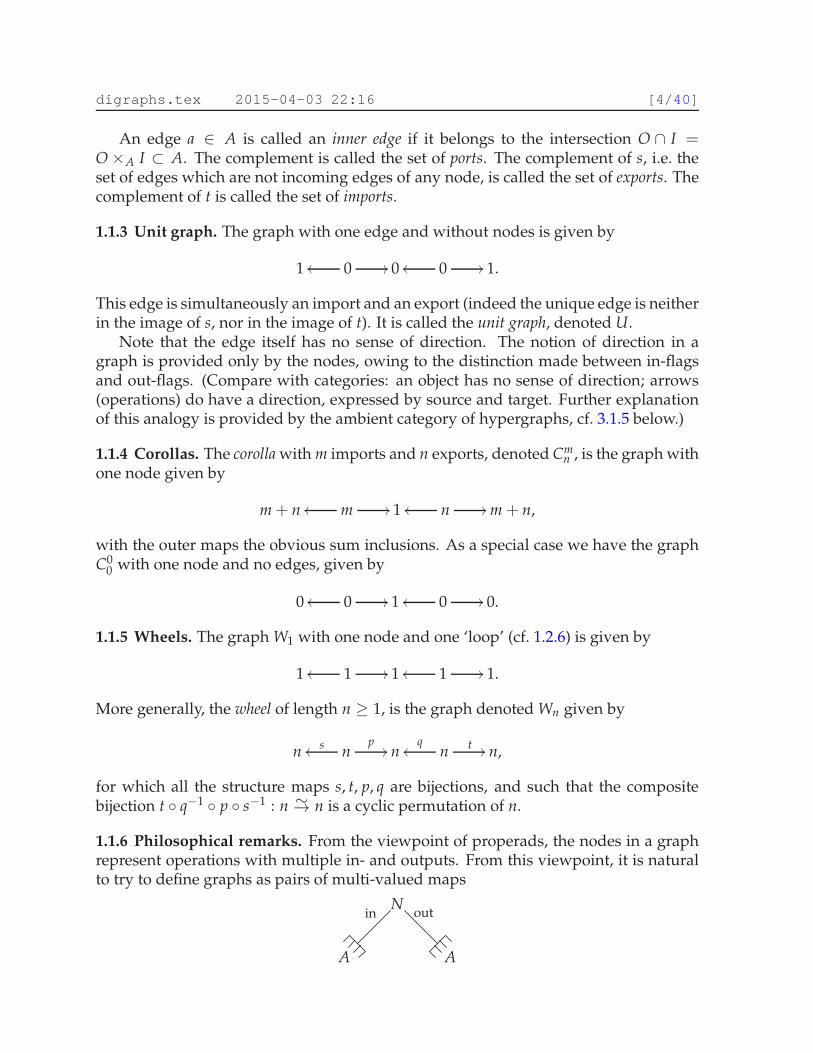
1.1.3 Unit graph. The graph with one edge and without nodes is given by

1 0oo // 0 0oo // 1.

This edge is simultaneously an import and an export (indeed the unique edge is neitherin the image of s, nor in the image of t). It is called the unit graph, denoted U.

Note that the edge itself has no sense of direction. The notion of direction in agraph is provided only by the nodes, owing to the distinction made between in-flagsand out-flags. (Compare with categories: an object has no sense of direction; arrows(operations) do have a direction, expressed by source and target. Further explanationof this analogy is provided by the ambient category of hypergraphs, cf. 3.1.5 below.)

1.1.4 Corollas. The corolla with m imports and n exports, denoted Cmn , is the graph with

one node given by

m + n moo // 1 noo // m + n,

with the outer maps the obvious sum inclusions. As a special case we have the graphC0

0 with one node and no edges, given by

0 0oo // 1 0oo // 0.

1.1.5 Wheels. The graph W1 with one node and one ‘loop’ (cf. 1.2.6) is given by

1 1oo // 1 1oo // 1.

More generally, the wheel of length n ≥ 1, is the graph denoted Wn given by

n nsoop

// n nq

oo t // n,

for which all the structure maps s, t, p, q are bijections, and such that the compositebijection t ◦ q−1 ◦ p ◦ s−1 : n ∼→ n is a cyclic permutation of n.

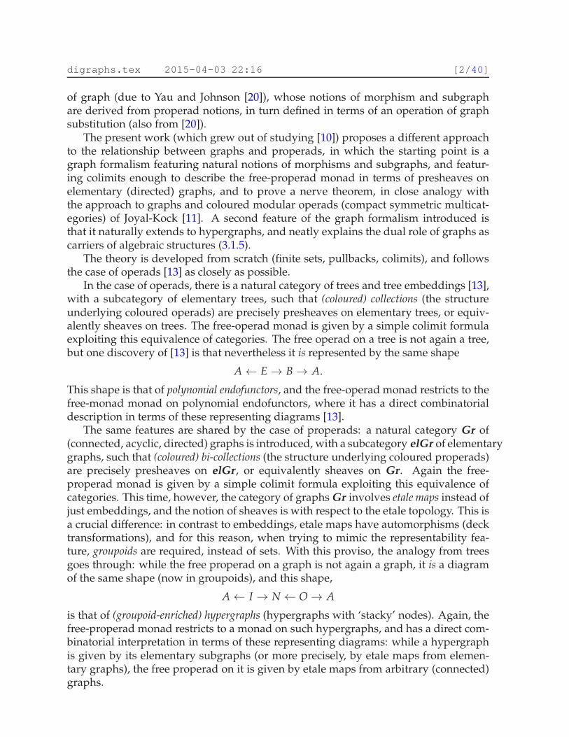
1.1.6 Philosophical remarks. From the viewpoint of properads, the nodes in a graphrepresent operations with multiple in- and outputs. From this viewpoint, it is naturalto try to define graphs as pairs of multi-valued maps

N

A A

in out

digraphs.tex 2015-04-03 22:16 [5/40]

A standard way to encode a multi-valued map is as a span. Hence we arrive at theshape (1).

On the other hand, since a closed directed graph is an endospan E ⇒ V (source andtarget of an edge), a directed graph admitting open-ended edges should be the samebut with just partially defined maps. A standard way to encode a partially definedmap is as a span in which the backward arrow is an injection, hence again we arrive atour shape of diagrams for a graph.

These dual viewpoints also point towards the natural relationship with hyper-graphs: the shape is naturally the juxtaposition of the incidence relations a-hyperedge-being-the-input-of-a-node and a-hyperedge-being-the-output-of-a-node, which is oneway to represent directed hypergraphs, cf. 3.1.1 below.

A main feature and motivation for the present graph implementation are the ele-gant notions of morphisms that follow from the definition.

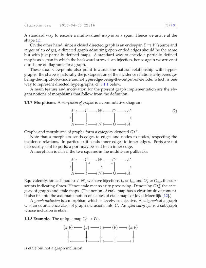
1.1.7 Morphisms. A morphism of graphs is a commutative diagram

A′

�

I ′oo

��

// N′

��

O′oo

��

// A′

�

A Ioo // N Ooo // A

(2)

Graphs and morphisms of graphs form a category denoted Gr+.Note that a morphism sends edges to edges and nodes to nodes, respecting the

incidence relations. In particular it sends inner edges to inner edges. Ports are notnecessarily sent to ports: a port may be sent to an inner edge.

A morphism is etale if the two squares in the middle are pullbacks:

A′

�

I ′oo

��

❴✤

// N′

ϕ��

O′oo✤❴

��

// A′

�

A Ioo // N Ooo // A

Equivalently, for each node x ∈ N′, we have bijections I ′x ≃ Iϕx and O′x ≃ Oϕx, the sub-scripts indicating fibres. Hence etale means arity preserving. Denote by Gr+et the cate-gory of graphs and etale maps. (The notion of etale map has a clear intuitive content.It also fits into the axiomatic notion of classes of etale maps of Joyal-Moerdijk [12].)

A graph inclusion is a morphism which is levelwise injective. A subgraph of a graphG is an equivalence class of graph inclusions into G. An open subgraph is a subgraphwhose inclusion is etale.

1.1.8 Example. The unique map C11 →W1,

{a, b}

��

{a}oo

��

// 1

��

{b}oo

��

// {a, b}

��

1 1oo // 1 1oo // 1

is etale but not a graph inclusion.

digraphs.tex 2015-04-03 22:16 [6/40]

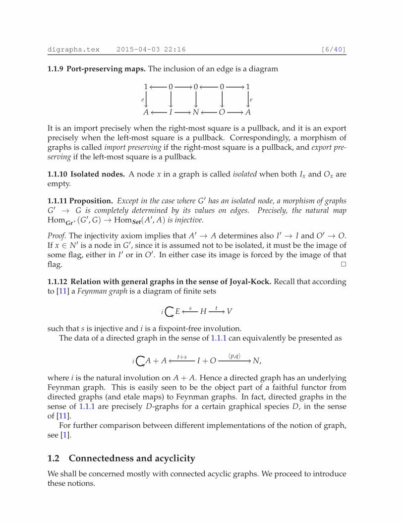
1.1.9 Port-preserving maps. The inclusion of an edge is a diagram

1

e��

0oo

��

// 0

��

0oo

��

// 1

e��

A Ioo // N Ooo // A

It is an import precisely when the right-most square is a pullback, and it is an exportprecisely when the left-most square is a pullback. Correspondingly, a morphism ofgraphs is called import preserving if the right-most square is a pullback, and export pre-serving if the left-most square is a pullback.

1.1.10 Isolated nodes. A node x in a graph is called isolated when both Ix and Ox areempty.

1.1.11 Proposition. Except in the case where G′ has an isolated node, a morphism of graphsG′ → G is completely determined by its values on edges. Precisely, the natural mapHomGr+(G

′, G)→ HomSet(A′, A) is injective.

Proof. The injectivity axiom implies that A′ → A determines also I ′ → I and O′ → O.If x ∈ N′ is a node in G′, since it is assumed not to be isolated, it must be the image ofsome flag, either in I ′ or in O′. In either case its image is forced by the image of thatflag. ✷

1.1.12 Relation with general graphs in the sense of Joyal-Kock. Recall that accordingto [11] a Feynman graph is a diagram of finite sets

Ei 88 Hsoo t // V

such that s is injective and i is a fixpoint-free involution.The data of a directed graph in the sense of 1.1.1 can equivalently be presented as

i 88A + A I + Ot+s

oo〈p,q〉

// N,

where i is the natural involution on A + A. Hence a directed graph has an underlyingFeynman graph. This is easily seen to be the object part of a faithful functor fromdirected graphs (and etale maps) to Feynman graphs. In fact, directed graphs in thesense of 1.1.1 are precisely D-graphs for a certain graphical species D, in the senseof [11].

For further comparison between different implementations of the notion of graph,see [1].

1.2 Connectedness and acyclicity

We shall be concerned mostly with connected acyclic graphs. We proceed to introducethese notions.

digraphs.tex 2015-04-03 22:16 [7/40]

1.2.1 Sums. The category Gr+ (as well as the subcategory Gr+et) has categorical sums,and the empty graph

0 0oo // 0 0oo // 0.

as initial object. Sums are calculated level-wise. They amount to disjoint union ofgraphs.

1.2.2 Connectedness. Recall that W1 is the graph 1 = 1 = 1 = 1 = 1 with one node andone loop (in fact the terminal object in Gr+ (but not in Gr+et)). A graph X is connected if

Hom(X, W1+W1) = 2.

In other words, X is non-empty and every morphism to W1+W1 is constant. Equiva-lently, X is non-empty and is not a sum of smaller graphs. (Equivalently, in its most cat-egorical formulation, a graph X is connected when Hom(X,−) preserves finite sums.)

1.2.3 Example. A graph for which all the structure maps are bijections is precisely adisjoint union of wheels. In fact the full subcategory spanned by graphs of this typeis equivalent to the category of finite-sets-with-a-permutation (by cycle-decompositionof permutations).

1.2.4 Acyclicity. A graph X is called acyclic (or wheel-free) if

Hom(Wn, X) = 0, ∀n > 0.

In other words, X does not admit a morphism from any wheel, or equivalently, doesnot contain a wheel as a subgraph.

1.2.5 Trees and linear graphs. An acyclic graph is a forest when q is a bijection. Anacyclic graph is a tree when q is a bijection and there is a unique export (compare [13]).It is a linear tree (or linear graph) if both p and q are bijections, and there is a uniqueexport. Denote by Lk the linear graph with k nodes.

1.2.6 Loops. A loop is an edge which is simultaneously an input and an output for thesame node. In other words, a ∈ A is a loop if there is a node x such that a ∈ Ix ∩Ox.Equivalently, a loop in X is the image edge of a map W1 → X. Accordingly, a node isloopfree if Ix + Ox → A is injective. A graph is loopfree if every node is loopfree. Fromthe W1-characterisation of loops, it is clear that an acyclic graph is loopfree.

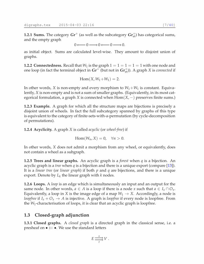
1.3 Closed-graph adjunction

1.3.1 Closed graphs. A closed graph is a directed graph in the classical sense, i.e. apresheaf on •⇔ •. We use the standard letters

Es //

t// V .

digraphs.tex 2015-04-03 22:16 [8/40]

To a closed graph is associated a graph in the sense of 1.1.1, namely

E E=oo t // V Esoo = // E.

This defines a fully faithful functor from closed graphs to graphs. Its essential imageis the subcategory of graphs for which the end maps are bijections. We also call theseclosed graphs.

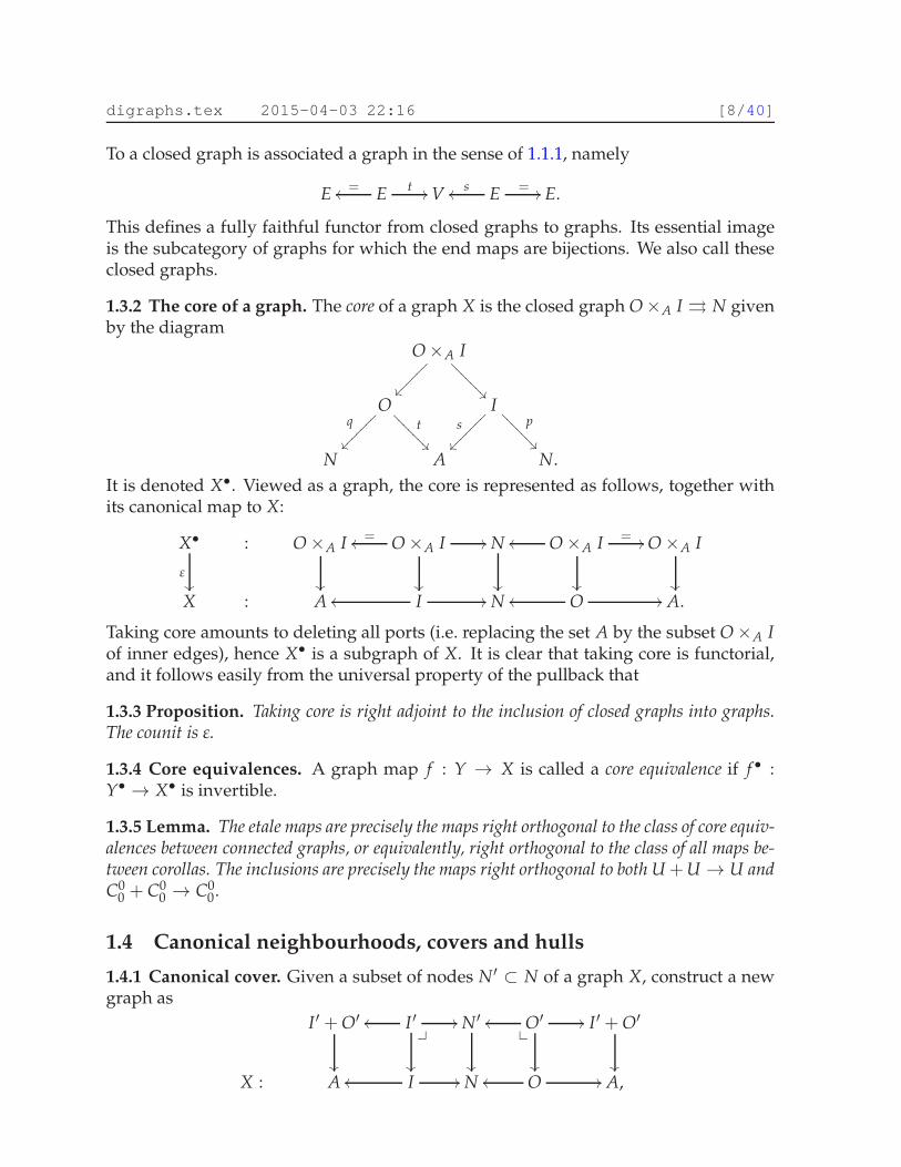
1.3.2 The core of a graph. The core of a graph X is the closed graph O×A I ⇒ N givenby the diagram

O×A I

��⑧⑧⑧⑧⑧⑧

��❄❄❄

❄❄❄❄

Oq

��⑧⑧⑧⑧⑧⑧⑧

t

��❄❄❄

❄❄❄❄

Is

��⑧⑧⑧⑧⑧⑧⑧ p

��❄❄❄

❄❄❄❄

N A N.It is denoted X•. Viewed as a graph, the core is represented as follows, together withits canonical map to X:

X•

�

: O×A I

��

O×A I=oo

��

// N

��

O×A Ioo

��

= // O×A I

��

X : A Ioo // N Ooo // A.

Taking core amounts to deleting all ports (i.e. replacing the set A by the subset O×A Iof inner edges), hence X• is a subgraph of X. It is clear that taking core is functorial,and it follows easily from the universal property of the pullback that

1.3.3 Proposition. Taking core is right adjoint to the inclusion of closed graphs into graphs.The counit is ε.

1.3.4 Core equivalences. A graph map f : Y → X is called a core equivalence if f • :Y• → X• is invertible.

1.3.5 Lemma. The etale maps are precisely the maps right orthogonal to the class of core equiv-alences between connected graphs, or equivalently, right orthogonal to the class of all maps be-tween corollas. The inclusions are precisely the maps right orthogonal to both U +U → U andC0

0 + C00 → C0

0 .

1.4 Canonical neighbourhoods, covers and hulls

1.4.1 Canonical cover. Given a subset of nodes N′ ⊂ N of a graph X, construct a newgraph as

I ′ + O′

��

I ′oo

��

❴✤

// N′

��

O′oo✤❴

��

// I ′ + O′

��

X : A Ioo // N Ooo // A,

digraphs.tex 2015-04-03 22:16 [9/40]

clearly a disjoint union of corollas. Jointly they cover the nodes in N′. When N′ = N,this is called the canonical etale cover of X, denoted cancov(X). (It is an open cover iffX is loopfree.) When N′ consists of a single node x ∈ N, the construction gives thecanonical neighbourhood of x, an open subgraph when x is loopfree.

1.4.2 Open hull. In the same situation, the open hull of N′ is defined by gluing theedges of the corollas according to their incidences in X, to obtain an open subgraph inX. The notion of gluing will be formalised below. In the present situation, it meanstaking union inside A instead of disjoint union: simply take the image factorisationof I ′ + O′ → A. Note that this includes also any existing loops at the nodes. By theuniversal property of union, it is the smallest open subgraph having N′ as set of nodes.

1.4.3 Etale hull. Slightly more involved is the construction of the etale hull of a subgraph.In this situation we are given a subgraph G ⊂ X, and we want to factor the inclusionas a core equivalence followed by an etale map. The construction of flags is as before(forced by the etale requirement). It remains to construct the correct edge set: it isa certain pushout, over the set of inner edges of G. It will be important to consider aslightly more general situation. A map of graphs X′ → X is called locally injective whenfor each x ∈ N′ we have that I ′x → Iϕx and O′x → Oϕx are injective.

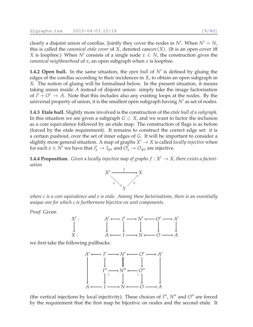
1.4.4 Proposition. Given a locally injective map of graphs f : X′ → X, there exists a factori-sation

X′f

//

c ❅

❅❅❅❅

❅❅❅ X

Y

e

??⑧⑧⑧⑧⑧⑧⑧⑧

where c is a core equivalence and e is etale. Among these factorisations, there is an essentiallyunique one for which c is furthermore bijective on unit components.

Proof. GivenX′ :

��

A′

��

I ′oooo

��

// N′

��

O′oo

��

// // A′

��

X : A Ioooo // N Ooo // // A

we first take the following pullbacks:

A′

��

I ′oooo��

��

// N′ O′oo��

��

// // A′

��

I ′′

��

❴✤

// N′′

��

O′′oo✤❴

��

A Ioooo // N Ooo // // A

(the vertical injections by local injectivity). These choices of I ′′, N′′ and O′′ are forcedby the requirement that the first map be bijcetive on nodes and the second etale. It

digraphs.tex 2015-04-03 22:16 [10/40]

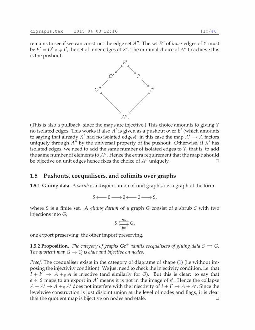
remains to see if we can construct the edge set A′′. The set E′′ of inner edges of Y mustbe E′ = O′×A′ I ′, the set of inner edges of X′. The minimal choice of A′′ to achieve thisis the pushout

E′��

��⑧⑧⑧⑧⑧ ��

��❄❄❄

❄❄

O′��

��⑧⑧⑧⑧⑧

I ′��

��❄❄❄

❄❄

O′′��

��❄❄❄

❄❄❄❄

❄❄❄❄

❄❄❄

I ′′��

��⑧⑧⑧⑧⑧⑧⑧⑧⑧⑧⑧⑧⑧⑧

A′′.

(This is also a pullback, since the maps are injective.) This choice amounts to giving Yno isolated edges. This works if also A′ is given as a pushout over E′ (which amountsto saying that already X′ had no isolated edges): in this case the map A′ → A factorsuniquely through A′′ by the universal property of the pushout. Otherwise, if X′ hasisolated edges, we need to add the same number of isolated edges to Y, that is, to addthe same number of elements to A′′. Hence the extra requirement that the map c shouldbe bijective on unit edges hence fixes the choice of A′′ uniquely. ✷

1.5 Pushouts, coequalisers, and colimits over graphs

1.5.1 Gluing data. A shrub is a disjoint union of unit graphs, i.e. a graph of the form

S 0oo // 0 0oo // S,

where S is a finite set. A gluing datum of a graph G consist of a shrub S with twoinjections into G,

S// ex ////

im// G,

one export preserving, the other import preserving.

1.5.2 Proposition. The category of graphs Gr+ admits coequalisers of gluing data S ⇒ G.The quotient map G→ Q is etale and bijective on nodes.

Proof. The coequaliser exists in the category of diagrams of shape (1) (i.e without im-posing the injectivity condition). We just need to check the injectivity condition, i.e. thatI + I ′ → A +S A is injective (and similarly for O). But this is clear: to say thate ∈ S maps to an export in A′ means it is not in the image of s′. Hence the collapseA + A′ → A +S A′ does not interfere with the injectivity of I + I ′ → A + A′. Since thelevelwise construction is just disjoint union at the level of nodes and flags, it is clearthat the quotient map is bijective on nodes and etale. ✷

digraphs.tex 2015-04-03 22:16 [11/40]

1.5.3 Corollary. The category Gr+et of graphs and etale maps admits coequalisers of gluingdata.

The colimit of a gluing datum S ⇒ G is constructed by connecting exports to im-ports in G, realising one connection for each unit graph in S. Although it is a trivialobservation, it will be important to note that this colimit can be computed in steps byrealising the connections one by one in any order.

1.5.4 Elementary graphs. An elementary graph is a connected graph without inneredges. Up to isomorphism there are only the following: the unit graph (one edge, nonodes), and the (m, n)-corollas. Let elGr ⊂ Gret denote the full subcategory spannedby the elementary graphs (and all etale maps). Hence the only maps are the inclusionsof an edge into a corolla, and the permutations of imports or exports.

1.5.5 Elements. Let X be a graph A Isoo

p// N O

qoo t // A. The comma cate-

gory el(X) := elGr↓X is called the category of elements of X. (See [15], Ch.II, §6, for thenotion of comma category.) It has the following explicit description. Its object set isA + N. Its set of non-identity arrows is I + O. An element f ∈ I has domain s( f ) andcodomain p( f ); an element g ∈ O has domain t(g) and codomain q(g). Since everyarrow goes from an object in A to an object in N, the category is really just a bipartitegraph (with identity arrows added), namely the barycentric subdivision of X.

The category of elements el(X) indexes canonically a diagram of elementary graphs,el(X) → Gr+, and X is the colimit of this diagram in Gr+:

X = colimE∈el(X)

E = colim(

el(X) → Gr+). (3)

Assuming that X has no unit components, the outer edges play no role in the col-imit: it can be computed equally well indexed over el(X•) ⊂ el(X) (although of coursethe ingredient elementary graphs are those of X, not those of X•). The colimit indexedover el(X•) is that of a gluing datum: it is the coequaliser of the canonical cover (thedisjoint union of all the nodes in X considered as corollas, cf. 1.4.1) over the inneredges:

O×A I ⇒ cancov(X) → X.

More generally, we have:

1.5.6 Lemma. For X a graph without unit components, the functor el(X•)→ el(X) is final.

1.5.7 Corollary. If X → Y is a core equivalence between graphs without unit components,then el(X) → el(Y) is final.

See [15], Ch.IX, §3, for the notion of final functor. What this amounts to is that if f :el(X) → C is a functor, and if el(X•) → el(X) → C admits a colimit, then so does f ,and the two colimits agree.

digraphs.tex 2015-04-03 22:16 [12/40]

1.5.8 Gluing datum from a graph of graphs. The case of interest in the previous dis-cussion is the following. A functor el(X) → Gr+ is called a graph of graphs if it sendsall A-objects to unit graphs, and all I-maps to import-preserving maps and all O-mapsto export-preserving maps. In this case (unless X is has a unit component) the restric-tion to el(X•) is a gluing datum, and hence has a colimit. Therefore el(X) → Gr+

has a colimit. This is just the formal expression of the idea that if a graph X is deco-rated with graphs at the nodes, then the decorating graphs (one for each node) can beglued together as prescribed by the incidence relations in the indexing graph. (In theliterature, this situation (subject to a further compatibility condition, see 2.3.2) is oftenreferred to as graph substitution (see for example [1] or [20]): the colimit is interpretedas the result of substituting each decorating graph into the corresponding node of theindexing graph.)

1.5.9 Colimit formula for etale hull. If H → G is a subgraph, then the etale hull (1.4.3)is given by

colim(

el(H)→ el(G)→ Gr+).

This just says that the etale hull is obtained by gluing together corollas from G accord-ing to the shape of H.

1.5.10 Residue. Denote by Cor the full subcategory of Gret consisting of the corollas.Clearly Cor is a groupoid. The residue of a connected graph G is the corolla having thesame imports and exports as G. This defines a functor res : Gr iso → Cor (functorial inisomorphisms, not in general maps). Note that res(U) = C1

1 . If x is a node of a graph,we shall also write res(x) for the residue of the canonical neighbourhood of x.

1.5.11 Indexing graph for a gluing datum. A coequaliser of a gluing datum S ⇒ Gcan be interpreted as a colimit of connected graphs as follows. Write S and G as sumsof connected components

∑i

Ui ⇒ ∑k

Gk.

Form the graph ∑ Rk by replacing each Gk with its residue Rk = res(Gk). We still havethe maps from the S edges into these corollas, and we can take the colimit R, whichwe call the indexing graph. The original diagram is now over el(R•), the category ofelements of R•.

1.5.12 Lemma. The coequaliser Q is connected if and only if the indexing graph R is con-nected. Furthermore, in this situation, res(Q) ≃ res(R).

Proof. To give a map Q → W1 + W1 is the same as giving a cocone S ⇒ ∑ Gk → W1 +W1. Since each of the Gk is connected, each map Gk → W1 + W1 is constant, and henceamounts to giving a cocone S ⇒ ∑ Rk → W1 + W1, and hence a map R → W1 + W1.Hence Q is connected if and only if R is. The second statement follows easily since byconstruction ∑ Gk and ∑ Rk have the same set of imports, of which the same subset Sis spent with gluing, so that also Q and R are left with the same set of imports. Dittowith exports. ✷

digraphs.tex 2015-04-03 22:16 [13/40]

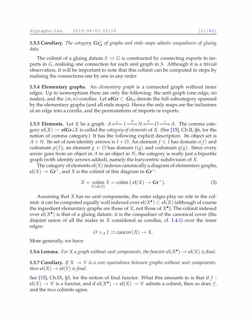
1.5.13 Lemma. If all the individual graphs Gk are acyclic, and if the indexing graph R isacyclic then the coequaliser Q is acyclic too.

Proof. Let W → Q be a wheel in Q. For each of the connected graphs Gk, consider thepullback

Hk❴✤

//

��

Gk

��

W // Q

Since we have assumed Gk acyclic, each Hk is a sum of linear graphs, and each Hk → Gk

preserves imports and exports. This means that it makes sense to take residue of eachHk → Gk, yielding in each case a map Tk → Rk = res(Gk), where each Tk is a sumof L1-graphs. These linear graphs L1 glue together to give a wheel in R. (It is closedbecause each import in one string corresponds to an export in another string.) ✷

1.5.14 Lemma. If the indexing graph R is loopfree, then each of the maps Gk → Q is an openinclusion.

1.6 Complements and convexity

The material in this subsection will only be needed again in Subsection 2.4.

1.6.1 Naive complement. If H → G is a subgraph (i.e levelwise injective), then thenaive complement is simply defined by taking complements levelwise. It is again a sub-graph. This notion is not very useful for the present purposes, where the emphasis inon etale maps. The better notion is the following adjustment.

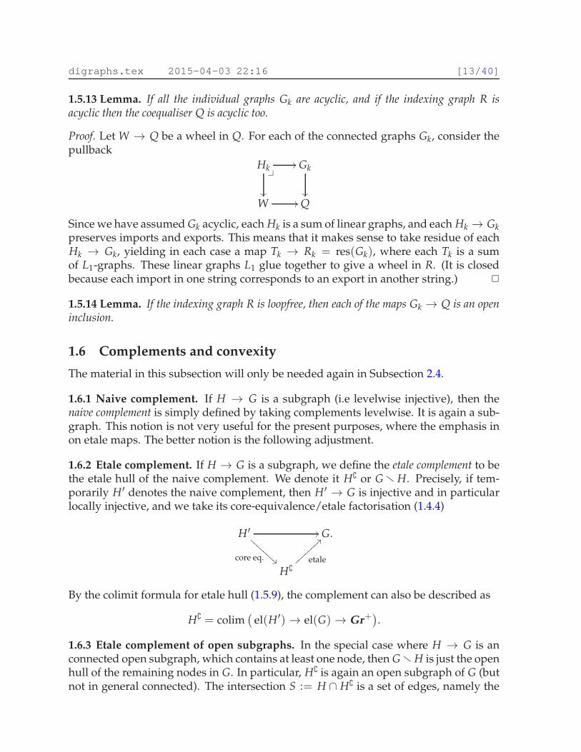
1.6.2 Etale complement. If H → G is a subgraph, we define the etale complement to bethe etale hull of the naive complement. We denote it H∁ or Gr H. Precisely, if tem-porarily H′ denotes the naive complement, then H′ → G is injective and in particularlocally injective, and we take its core-equivalence/etale factorisation (1.4.4)

H′ //

core eq. ❇❇❇

❇❇❇❇

❇ G.

H∁

etale

>>⑥⑥⑥⑥⑥⑥⑥⑥

By the colimit formula for etale hull (1.5.9), the complement can also be described as

H∁ = colim(

el(H′)→ el(G) → Gr+).

1.6.3 Etale complement of open subgraphs. In the special case where H → G is anconnected open subgraph, which contains at least one node, then Gr H is just the openhull of the remaining nodes in G. In particular, H∁ is again an open subgraph of G (butnot in general connected). The intersection S := H ∩ H∁ is a set of edges, namely the

digraphs.tex 2015-04-03 22:16 [14/40]

ports of H that are not also ports of G, and G can be recovered by gluing together Hand H∁ along S. Precisely, G is naturally the colimit of the gluing datum

S ⇒ H + H∁. (4)

1.6.4 Etale complement of an edge. We shall also need the very special case where Hconsists of a single edge of G. If H consists of a port of G, then H∁ = G. If H consistsof an inner edge e of G, then Gr e is the graph obtained from G by cutting that edge.More formally, just as G is the colimit of the canonical gluing datum

O×A I ⇒ cancovG

(of all the nodes over all the inner edges), Gr e is the colimit of

O×A I r e ⇒ cancovG.

Hence there is a natural map Gr e → G which is bijective on nodes and etale but notan inclusion: the inverse image of e consists of two edges.

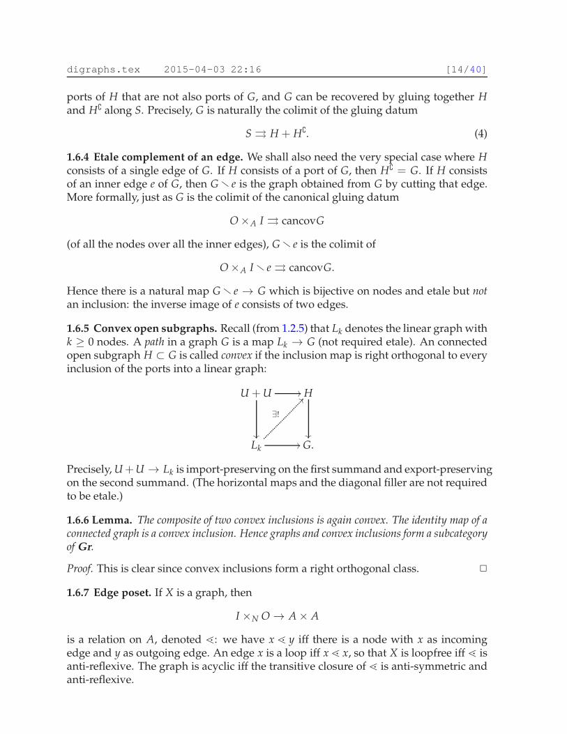
1.6.5 Convex open subgraphs. Recall (from 1.2.5) that Lk denotes the linear graph withk ≥ 0 nodes. A path in a graph G is a map Lk → G (not required etale). An connectedopen subgraph H ⊂ G is called convex if the inclusion map is right orthogonal to everyinclusion of the ports into a linear graph:

U + U //

��

H

��

Lk//

∃!

??

G.

Precisely, U +U → Lk is import-preserving on the first summand and export-preservingon the second summand. (The horizontal maps and the diagonal filler are not requiredto be etale.)

1.6.6 Lemma. The composite of two convex inclusions is again convex. The identity map of aconnected graph is a convex inclusion. Hence graphs and convex inclusions form a subcategoryof Gr.

Proof. This is clear since convex inclusions form a right orthogonal class. ✷

1.6.7 Edge poset. If X is a graph, then

I ×N O→ A× A

is a relation on A, denoted ⋖: we have x ⋖ y iff there is a node with x as incomingedge and y as outgoing edge. An edge x is a loop iff x ⋖ x, so that X is loopfree iff ⋖ isanti-reflexive. The graph is acyclic iff the transitive closure of ⋖ is anti-symmetric andanti-reflexive.

digraphs.tex 2015-04-03 22:16 [15/40]

Assuming that X is acyclic, the transitive and reflexive closure of ⋖, denoted≤, is aposet called the edge poset of X. We have x ≤ y iff there is a path from x to y in the graph.Hence a connected open subgraph H ⊂ X is convex iff the edge poset of H is a convexsubset of the edge poset of X, in the usual sense (x, y ∈ H & x ≤ m ≤ y⇒ m ∈ H).

1.6.8 Remark. The notion of convexity makes sense of course also for subgraphs notrequired to be open or not required to be connected, but then a looser notion of pathis needed to detect convexity: specifically, ‘linear’ graphs starting or ending in a nodeinstead of an edge should be allowed

Conversely, it is also possible to formulate the notion of convexity entirely insidethe category of etale maps. In this case the notion of path must be replaced by thenotion of strip: a strip is the etale hull of a path. In the lifting diagram, instead of justlinear graphs Lk it is necessary to use all the graphs P such that P• ≃ L•k . Indeed, theseare precisely the graphs that can appear in the core-equivalence/etale factorisation ofa path, as in 1.4.4.

1.6.9 Convexity in terms of etale complements. Let H be a connected open subgraphof an acyclic graph G. If H is a single edge, clearly H is convex. So we assume nowthat H contains at least one node. The intersection S := H ∩ H∁ is a disjoint union ofedges. Convexity says that there are no paths starting and ending in H that go througha node of H∁. Such an offending path must necessarily go through an edge in S (wemust leave H somewhere), then through at least one node in H∁, and later throughanother edge in S (we must enter H again somewhere). So equivalently we can saythat there is no path in H∁ between two distinct edges of S. In particular, we see thatconvexity of H does not really depend on what is inside H, but only on its boundaryand its relationship with the complement.

1.6.10 Terminology from Hackney-Robertson-Yau [10]. Two important notions in [10]can be expressed in terms of convexity: Two nodes in a connected graph are closestneighbours [20], when the open hull of the two nodes is (connected and) convex. Anode of a connected graph is almost isolated if the complement is (connected and) con-vex, or if it is the only node in the graph. (The reader is referred to [10] to see howthese notions are defined there (without the notion of convexity), and how they areexploited, among other things, to arrive at the notion of subgraph used there (whichin the present terminology is the notion of convex open subgraph).)

2 Properads

This section owes a lot to Joyal-Kock [11].

Denote by Gr the category of connected acyclic graphs with etale maps. From nowon we say simply graph for connected acyclic graph.

digraphs.tex 2015-04-03 22:16 [16/40]

2.1 Digraphical species (coloured bi-collections) and F-graphs

2.1.1 Digraphical species = coloured bi-collections. A presheaf

F : elGrop −→ Set

E 7−→ F[E]

is called a digraphical species or a (coloured) bi-collection. So it is the data of a ’set ofcolours’ F[U], the value on the unit graph, and for each (m, n), a set F[m, n] of oper-ations of biarity (m, n). Each input and output slot in an operation is labelled by acolour, via the maps in elGr from the unit graph to the corollas.

We favour the terminology digraphical species when F conveys the idea of a structureon digraphs, something to decorate digraphs with, while we prefer the terminology bi-collection when F serves as the structure underlying (or freely generating) a properad.

A graph X defines a bi-collection by

X : elGrop −→ Set

E 7−→ Homet(E, X).

The category of elements el(X) introduced in 1.5.5 then coincides with the category ofelements of this presheaf (see [15], Ch.III, §7).

2.1.2 Grothendieck topology and sheaves. The category Gr has a natural Grothendiecktopology in which a cover is a collection of etale maps that are jointly surjective onnodes and on edges. Every graph has a canonical cover cancov(X) → X which is adisjoint union of elementary graphs, cf. 1.4.1. From (3) we get

PrSh (elGr) ≃ Sh (Gr).

Via this equivalence, a digraphical species F can be evaluated on any graph, notjust on the elementary ones. The formula is:

F[G] = limE∈el(G)

F[E].

(We already know that G is a colimit of its canonical diagram, in the category Gr ofgraphs and etale maps. That F is a sheaf on Gr means precisely that this colimit is sentto a limit, which is the one in the formula.)

2.1.3 Lemma. In the special case where the presheaf F : elGrop → Set is ‘represented’ bya graph X, that is, F[E] = Homet(E, X), then as a sheaf F : Grop → Set it is genuinelyrepresented by X:

F[G] = Homet(G, X).

Proof.

F[G] = limE∈el(G)

F[E] = limE∈el(G)

Homet(E, X) = Homet(colim E, X) = Homet(G, X).✷

digraphs.tex 2015-04-03 22:16 [17/40]

2.1.4 F-graphs. Every digraphical species F defines a notion of F-graph. They aregraphs whose edges are decorated by the colours of F, and whose nodes are deco-rated by the operations of F, subject to obvious compatibility conditions. Formally,the category of F-graphs is the comma category Gr↓F (or Gr+↓F if we allow non-connected graphs). If for a moment we denote by T the terminal digraphical species,then T-graphs are the same thing as graphs, in the following discussion called nakedgraphs.

All the basic results about graphs hold also for F-graphs. Coequalisers of gluingdata exist for F-graphs, just as for graphs, now over F-shrubs, but the indexing graphis a naked graph, not an F-graph: the residue of an F-graph is not naturally an F-graph,only a naked graph. (For example, F could be the (2, 1)-species, whose F-graphs arebinary trees. The residue of a binary tree is of course not in general a binary tree.)Similarly, a graph of F-graphs el(R) → Gr+↓F admits a colimit in Gr+↓F (obtained bygluing together all the F-graphs according to the incidence relations expressed by thenaked graph R).

(Again we see that the indexing graph is not on the same footing as the ingredientsof the colimit. There is no natural notion of substituting an F-graph into the nodeof a naked graph. What does make sense is to use the naked graph as a shape ofcolimit to compute in the category Gr+↓F. It’s a recipe for gluing. Hence in the presentformalism, gluing is the fundamental notion, while substitution is derived from it.)

2.2 The free-properad monad

We shall define properads as algebras for a certain monad. This properad monad wasalso described by Hackney-Robertson-Yau [10] (Ch.2), and in a more general setting byYau-Johnson [20] (Ch.10–11), in both cases in terms of graph substitution. The presentdescription of the monad is literally the same as that for coloured modular operads ofJoyal-Kock [11], where in turn it is mentioned that it is just the coloured version of theconstruction of Getzler-Kapranov [9].

2.2.1 (m, n)-graphs. An (m, n)-graph is a graph G equipped with an isomorphismres(G) ≃ Cm

n . More formally, the groupoid of (m, n)-graphs (m, n)-Gr iso is the ho-motopy fibre over Cm

n of the functor res : Gr iso → Cor . Note that res : Gr iso → Coris a groupoid fibration, not a discrete fibration, since a graph may well have automor-phisms that fix all ports. We are interested in its fibrewise π0: that’s the essential partof a digraphical species, which to (m, n) assigns π0((m, n)-Gr iso). (It does not say any-thing about colours, the values on the unit graph, but this information will be providedautomatically in the construction below.)

If F is a digraphical species, there is a residue functor res : Gr iso↓F → Cor fromF-graphs to naked corollas. The groupoid of (m, n)-F-graphs, denoted (m, n)-Gr iso↓F,is the homotopy fibre over Cm

n of this functor.

digraphs.tex 2015-04-03 22:16 [18/40]

2.2.2 Underlying endofunctor of the free-properad monad. Let ppp denote the unitgraph. We define the monad for properads:

PrSh (elGr) −→ PrSh (elGr)

F 7−→ F,

where F is the bi-collection given by F[ ppp ] := F[ ppp ] and

F[m, n] := colimG∈(m,n)-Griso

F[G]

= ∑G∈π0((m,n)-Griso)

F[G]

Aut(m,n)(G)

= π0((m, n)-Gr iso↓F

).

Here the first equation follows since (m, n)-Gr iso is just a groupoid: the sum is over iso-morphism classes of (m, n)-graphs, and Aut(m,n)(G) denotes the automorphism groupof G in (m, n)-Gr iso.

2.2.3 Multiplication for the monad. F[m, n] is the set of isomorphism classes of (m, n)-F-graphs: it is the set of ways to decorate (m, n)-graphs by the digraphical species F.Now F[m, n] is the set of (m, n)-graphs decorated by F-graphs: this means that eachnode is decorated by an F-graph with matching ports. We can use the (m, n)-graph asindexing a diagram of F-graphs, and then take the colimit. This describes the monadmultiplication

µF : F → F.

More formally, the groupoid Gr iso↓F has as objects pairs (R, φ) where R is a graph,and φ : Hom(−, R) → F is a natural transformation. Equivalently we can regard φas a functor el(R) → elGr↓F. Now there is also a canonical functor elGr↓F → Gr↓F,which takes unit graphs to unit graphs, and takes a corolla decorated by an F-graph tothat same F-graph. The composite functor

el(R) → elGr↓F → Gr↓F

is a graph of F-graphs in the technical sense of 1.5.8, and we take its colimit to obtain asingle F-graph. The whole construction defines a functor

Gr iso↓F → Gr iso↓F,

which is compatible with taking residue by Lemma 1.5.12. The fibrewise π0 of thisfunctor defines the monad multiplication.

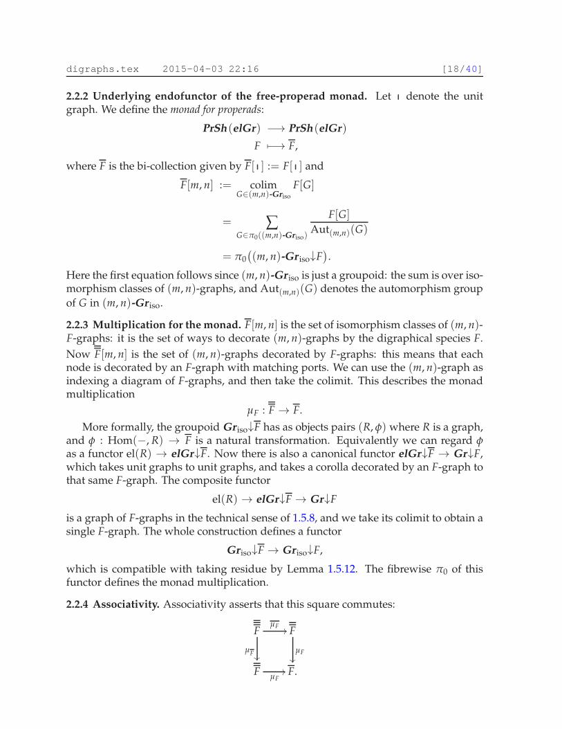
2.2.4 Associativity. Associativity asserts that this square commutes:

FµF

//

µF��

F

µF

��

FµF

// F.

digraphs.tex 2015-04-03 22:16 [19/40]

The elements in F[m, n] are graphs of graphs of F-graphs, and associativity amountsto saying that these F-graphs can be glued together in two ways with the same result.

In detail, an element in F[m, n] is a graph of F-graphs, so it amounts to a graph R, andfor each node x in R an F-graph Ax (and for each inner edge in R the correspondingports of the Ax match). Each F-graph Ax is a graph of F-graphs, so for each nodein each Ax there is an F-graph (and again compatibilities). So altogether there is anumber of F-graphs involved; associativity says that the following two ways of gluingthem all together give the same result. Either inner-first (that’s µF ◦ µF): we first gluetogether, for each Ax separately, the corresponding F-graphs, to obtain a set of biggerF-graphs indexed by the nodes in R, and then finally glue together these bigger F-graphs according to the colimit shaped by R. Or outer-first (that’s µF ◦ µF): we firstprepare the overall shape by gluing together all the graphs Ax according to the shapeR. This produces a graph Q of F-graphs, and then we use Q as recipe for gluing all theF-graphs. Note that there is a natural bijection between the nodes in Q and the sumof all the nodes in all the Ax — this follows because the quotient map of the gluingconstruction S ⇒ ∑x Ax → Q is bijective on nodes (1.5.2). To see that the two gluingconstructions agree, assume first that none of the Ax are unit graphs. Start with theouter-first gluing: here we are simply gluing all the F-graphs according to one graphQ. However, this graph Q contains as open subgraphs all the Ax. We can perform thecolimit construction by first gluing separately over the inner edges of each of the Ax

(in each case this is a subset of the inner edges in Q, and all these subsets are disjoint).But this first step is precisely to assemble all the F-graphs according to which Ax theybelong to, so it is precisely the first step in the inner-first gluing prescription. Finallywe glue along the remaining inner edges in Q. By the assumption that none of theAx are unit graphs, these remaining inner edges are precisely identified with the inneredges of the outermost graph R. So under this assumption, both ways of gluing areover the same sets of edges. Finally we can easily reduce to this situation from thegeneral case: if there is a node x in R such that Ax is a unit graph, then we can startthe colimit computation (in either way) by taking the pushout over any inner edgeincident to x. This pushout does not affect the result, neither the graph Q in the outer-first calculation, nor the gluing of the F-graphs Ax in the inner-first calculation. Wemay therefore as well assume that there are no nodes of this type in R.

2.2.5 Unit for the monad. The unit for the monad is given by interpreting an F-corollaC ∈ F[m, n] as an F-graph. The unit law says: (1) given an (m, n)-F-graph X, interpret-ing it first as an (m, n)-corolla of F-graphs (the single F-graph X itself), and then takingthe (trivial) colimit, that gives back the F-graph X again; and (2), interpreting X as agraph of F-corollas, and then taking the colimit of these corollas, also gives back theoriginal F-graph X. Both cases are clear.

2.2.6 Properads. A (coloured) properad is defined to be an algebra for the properadmonad F 7→ F. This means that it is a bi-collection F : elGrop → Set equipped with astructure map F → F obeying a few easy axioms (cf. [15], Ch. VI): it amounts to a rulewhich for any (m, n)-graph G gives a map F[G] → F[m, n], i.e. a way of constructing

digraphs.tex 2015-04-03 22:16 [20/40]

a single operation from a whole graph of them. This rule satisfies some associativityconditions, amounting to independence of the different ways of breaking the compu-tation into steps. Let Prpd denote the category of algebras for the properad monadF 7→ F.

2.2.7 Some variations. Polycategories [16], also called dioperads [7], are obtained byusing only simply connected graphs (and the same elementary graphs). Operads areobtained by using only rooted trees (and then only elementary graphs that are rootedtrees), cf. 1.2.5. See Kock [13]. Categories are obtained by using only linear graphs (andelementary graphs that are linear).

2.3 Generic/free factorisation and nerve theorem

This subsection and the next, not really used elsewhere in the paper, introduce andstudy a bigger category of graphs, whose new maps are generated by the free-properadmonad. One important aspect of this bigger category G̃r is the nerve theorem (2.3.9),characterising properads among presheaves on G̃r in terms of a Segal condition. Thecategory G̃r is also described by Hackney-Robertson-Yau [10], although they are moreinterested in a smaller category (see 2.4.14 below).

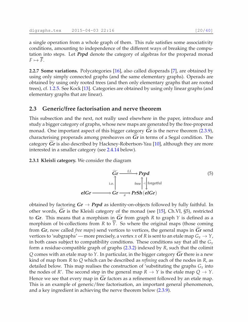
2.3.1 Kleisli category. We consider the diagram

G̃rf.f. // Prpd

forgetful��

⊣

elGr // Gr

i.o.

OO

a// PrSh (elGr)

free

OO(5)

obtained by factoring Gr → Prpd as identity-on-objects followed by fully faithful. Inother words, G̃r is the Kleisli category of the monad (see [15], Ch.VI, §5), restrictedto Gr. This means that a morphism in G̃r from graph R to graph Y is defined as amorphism of bi-collections from R to Y. So where the original maps (those comingfrom Gr , now called free maps) send vertices to vertices, the general maps in G̃r sendvertices to ‘subgraphs’ — more precisely, a vertex x of R is sent to an etale map Gx → Y,in both cases subject to compatibility conditions. These conditions say that all the Gx

form a residue-compatible graph of graphs (2.3.2) indexed by R, such that the colimitQ comes with an etale map to Y. In particular, in the bigger category G̃r there is a newkind of map from R to Q which can be described as refining each of the nodes in R, asdetailed below. This map realises the construction of ‘substituting the graphs Gx intothe nodes of R’. The second step in the general map R → Y is the etale map Q → Y.Hence we see that every map in G̃r factors as a refinement followed by an etale map.This is an example of generic/free factorisation, an important general phenomenon,and a key ingredient in achieving the nerve theorem below (2.3.9).

digraphs.tex 2015-04-03 22:16 [21/40]

2.3.2 Residue-compatible graphs of graphs. According to 1.5.8, a graph of F-graphsis a functor γ : el(R) → Gr↓F that sends all A-objects to unit F-graphs, and all I-maps to import-preserving maps and all O-maps to export-preserving maps. We saythat a graph of F-graphs γ is residue compatible when for each node x in R, we haveres(x) = res(γ(x)).

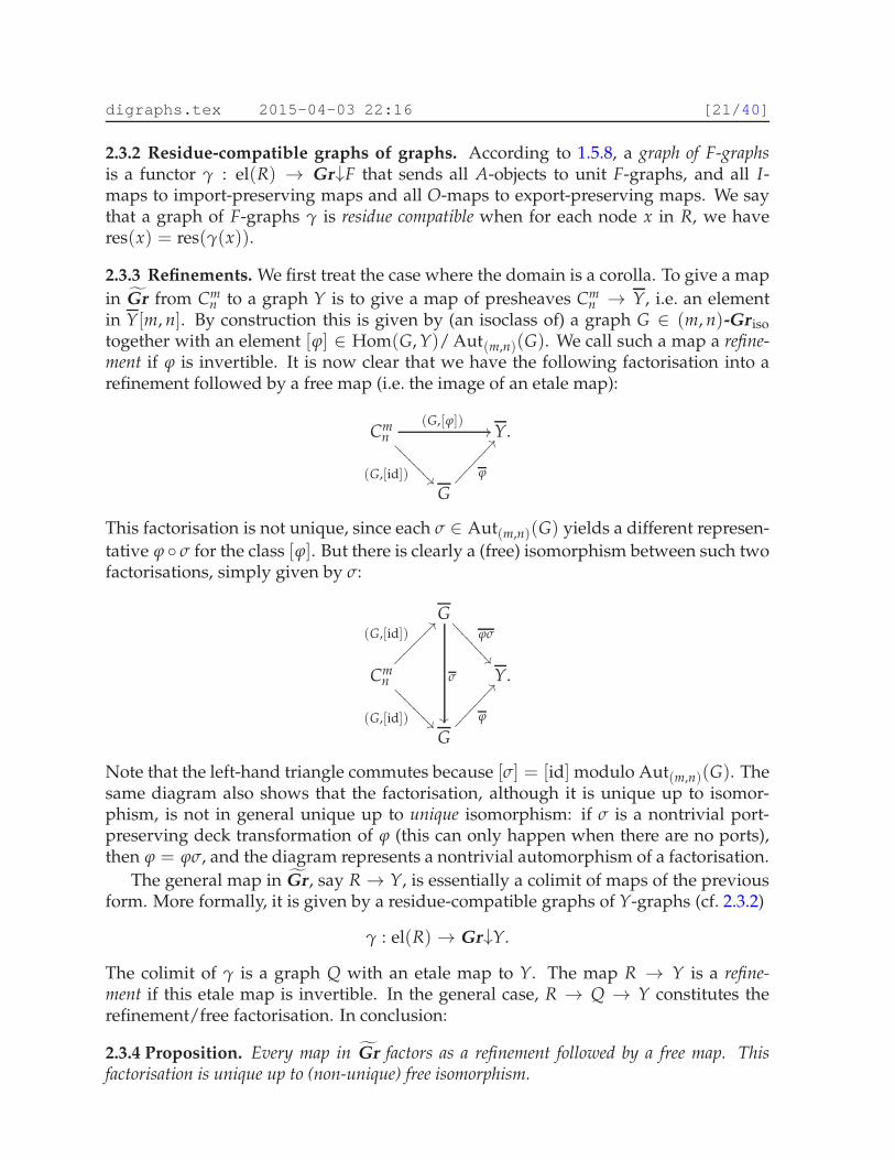
2.3.3 Refinements. We first treat the case where the domain is a corolla. To give a mapin G̃r from Cm

n to a graph Y is to give a map of presheaves Cmn → Y, i.e. an element

in Y[m, n]. By construction this is given by (an isoclass of) a graph G ∈ (m, n)-Gr isotogether with an element [ϕ] ∈ Hom(G, Y)/ Aut(m,n)(G). We call such a map a refine-ment if ϕ is invertible. It is now clear that we have the following factorisation into arefinement followed by a free map (i.e. the image of an etale map):

Cmn

(G,[ϕ])//

(G,[id])��❄

❄❄❄❄

❄❄❄

Y.

G

ϕ

@@✁✁✁✁✁✁✁✁

This factorisation is not unique, since each σ ∈ Aut(m,n)(G) yields a different represen-tative ϕ ◦ σ for the class [ϕ]. But there is clearly a (free) isomorphism between such twofactorisations, simply given by σ:

Gϕσ

��❂❂❂

❂❂❂❂

❂

σ

��

Cmn

(G,[id])??⑧⑧⑧⑧⑧⑧⑧⑧

(G,[id]) ��❄❄❄

❄❄❄❄

❄Y.

G

ϕ

@@✁✁✁✁✁✁✁✁

Note that the left-hand triangle commutes because [σ] = [id] modulo Aut(m,n)(G). Thesame diagram also shows that the factorisation, although it is unique up to isomor-phism, is not in general unique up to unique isomorphism: if σ is a nontrivial port-preserving deck transformation of ϕ (this can only happen when there are no ports),then ϕ = ϕσ, and the diagram represents a nontrivial automorphism of a factorisation.

The general map in G̃r , say R → Y, is essentially a colimit of maps of the previousform. More formally, it is given by a residue-compatible graphs of Y-graphs (cf. 2.3.2)

γ : el(R) → Gr↓Y.

The colimit of γ is a graph Q with an etale map to Y. The map R → Y is a refine-ment if this etale map is invertible. In the general case, R → Q → Y constitutes therefinement/free factorisation. In conclusion:

2.3.4 Proposition. Every map in G̃r factors as a refinement followed by a free map. Thisfactorisation is unique up to (non-unique) free isomorphism.

digraphs.tex 2015-04-03 22:16 [22/40]

A version of this factorisation is also obtained in [10] (Lemma 5.43).

2.3.5 Remark. In the preceding discussion, Y was assumed to be a graph, but it factthis is irrelevant: the arguments work exactly the same for Y a general presheaf. Inany case a map R → Y in the Kleisli category is given by γ : el(R) → Gr↓Y, subjectto the same conditions as above, and in any case the middle object Q appearing in thefactorisation R → Q → Y is a graph. This will be important in the proof of the nervetheorem.

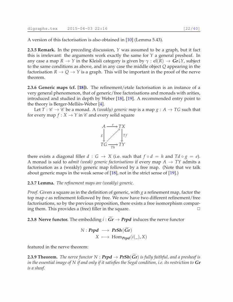
2.3.6 Generic maps (cf. [18]). The refinement/etale factorisation is an instance of avery general phenomenon, that of generic/free factorisations and monads with arities,introduced and studied in depth by Weber [18], [19]. A recommended entry point tothe theory is Berger-Melliès-Weber [4].

Let T : C → C be a monad. A (weakly) generic map is a map g : A → TG such thatfor every map f : X → Y in C and every solid square

Ae //

g

��

TX

T f

��

TGTh

//

??

TY

there exists a diagonal filler d : G → X (i.e. such that f ◦ d = h and Td ◦ g = e).A monad is said to admit (weak) generic factorisations if every map A → TY admits afactorisation as a (weakly) generic map followed by a free map. (Note that we talkabout generic maps in the weak sense of [18], not in the strict sense of [19].)

2.3.7 Lemma. The refinement maps are (weakly) generic.

Proof. Given a square as in the definition of generic, with g a refinement map, factor thetop map e as refinement followed by free. We now have two different refinement/freefactorisations, so by the previous proposition, there exists a free isomorphism compar-ing them. This provides a (free) filler in the square. ✷

2.3.8 Nerve functor. The embedding i : G̃r → Prpd induces the nerve functor

N : Prpd −→ PrSh (G̃r)

X 7−→ HomPrpd (i(_), X)

featured in the nerve theorem:

2.3.9 Theorem. The nerve functor N : Prpd→ PrSh(G̃r) is fully faithful, and a presheaf isin the essential image of N if and only if it satisfies the Segal condition, i.e. its restriction to Gris a sheaf.

digraphs.tex 2015-04-03 22:16 [23/40]

Proof. It is clear that Gr is small and that a : Gr → PrSh (elGr) is fully faithful anddense. The nerve theorem will be an instance of the general nerve theorem of We-ber [19] (Theorem 4.10), if just we can establish that a : Gr → PrSh (elGr) providesarities for the free-properad monad, which temporarily we denote by T. By Berger-Melliès-Weber [4] (Propositions 2.12–2.14), to say that a provides arities for T is equiv-alent to saying that the natural functor a↓Ta↓T → a↓T given by composition has con-nected fibres. The objects in a↓T are maps R → Y, where R is a graph and Y is anarbitrary presheaf. The fibre over a map R→ Y is the category of factorisations

R //

��❂❂❂

❂❂❂❂

❂ Y

Q

@@✁✁✁✁✁✁✁✁

such that the middle object is a graph, and the second map is free. But having (weak)generic factorisation say precisely that this factorisation category has a weakly initialobject, and in particular is connected. ✷

2.3.10 Remarks on the proof. Weber established the general nerve theorem ([19], The-orem 4.10) in the situation where T is a monad on a category C and a : Θ0 → C

provides arities for T. (To provide arities means that a certain left Kan extension ispreserved by the monad.) He showed furthermore ([19], Proposition 4.22) that if C isa presheaf category and T admits strict generic factorisations, then there is a canonicalchoice of Θ0, namely the full subcategory spanned by the objects that appear as mid-dle objects of generic/free factorisations of maps from a representable to the terminalpresheaf. It was observed in [13] (Remark 2.2.11) that the arguments in Weber’s proofin fact yield the more general criterion: a provides arities for T if the natural functora↓Ta↓T → a↓T has connected fibres and admits a section. Weber (personal commu-nication) pointed out that in fact the section is not necessary (although of course inpractice the section is often provided by generic factorisations). Finally, Berger-Melliès-Weber [4] (Propositions 2.12–2.14) turned the criterion into an if-and-only-if statement,and gave a more conceptual formulation and a more elegant proof, as part of a morestreamlined overall treatment.

2.3.11 Remarks on weak versus strict generic factorisations. Weber’s original notionof generic morphism was the weak notion [18], which is the one relevant in the presentwork. Subsequent work [19], [13], [4] focused on the strict notion, which is intimatelyrelated to the notion of local right adjoint. The weak/strict distinction is closely re-lated with the distinction between analytic and polynomial functors, which in fact wasWeber’s motivation for introducing the notions of generic map in the first place [18].

Although it is not a precise result at the time of this writing, it seems that in practicethe weak situation (related to weakly cartesian monads) always arises from truncationof a strict situation in a homotopical setting, a monad which is cartesian in the ho-motopical sense. This principle transpires from joint work with David Gepner [8] de-veloping the theory of polynomial functors and generic factorisations in ∞-categories,

digraphs.tex 2015-04-03 22:16 [24/40]

and observing in particular that in the ∞-world, the difference between analytic andpolynomial evaporates. (This and some related results are previewed in [14].)

The present case seems to corrobate this principle. The free-properad monad isonly weakly cartesian, due to the presence of the π0 in the formula for it. In Section 3.3below, a groupoid-valued version of the monad is described which avoids this trun-cation. I claim that the groupoid version of the free-properad monad is cartesian andis a local right adjoint, and that it therefore has strict generic factorisations (all in thehomotopy sense of [8]).

2.4 Working in the category G̃r .

The category G̃r is meant to contain all the combinatorics of graphs relevant to prop-erad theory. The subcategory Gr already has the ‘geometric part’: open inclusions,etale maps, symmetries, colimits. (In the following when we talk about colimits theyare understood to be in Gr.) The new maps introduced, the refinements, represent thealgebraic structure, embodying the substitution aspects. It is an important feature ofthe present approach that this category in which the two aspects interact is generatedby general machinery (such as presheaves and monads). While the abstract descriptionas a restricted Kleisli category was enough to establish the generic factorisations andthe nerve theorem, it is worthwhile, as we do in this subsection, to extract more explicitdescriptions of the refinement maps, and how they interact with the etale maps.

2.4.1 Lemma. Any map R→ Y in G̃r sends edges to edges.

Proof. Indeed, the map is given by a functor el(R) → Gr↓Y, assumed to be a residue-compatible graph of graphs in the technical sense of 2.3.2, and in particular it sendsA-objects of el(R) to unit Y-graphs, which is the same as saying that it sends edges toedges. ✷

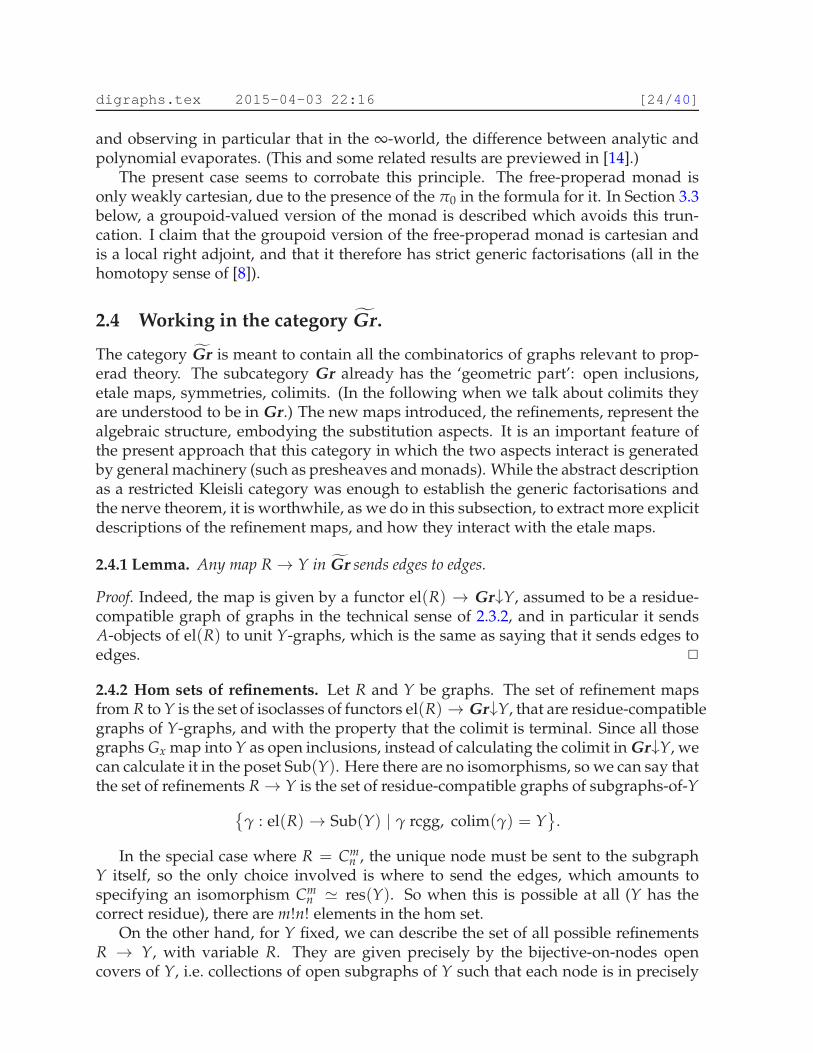
2.4.2 Hom sets of refinements. Let R and Y be graphs. The set of refinement mapsfrom R to Y is the set of isoclasses of functors el(R) → Gr↓Y, that are residue-compatiblegraphs of Y-graphs, and with the property that the colimit is terminal. Since all thosegraphs Gx map into Y as open inclusions, instead of calculating the colimit in Gr↓Y, wecan calculate it in the poset Sub(Y). Here there are no isomorphisms, so we can say thatthe set of refinements R→ Y is the set of residue-compatible graphs of subgraphs-of-Y

{γ : el(R) → Sub(Y) | γ rcgg, colim(γ) = Y

}.

In the special case where R = Cmn , the unique node must be sent to the subgraph

Y itself, so the only choice involved is where to send the edges, which amounts tospecifying an isomorphism Cm

n ≃ res(Y). So when this is possible at all (Y has thecorrect residue), there are m!n! elements in the hom set.

On the other hand, for Y fixed, we can describe the set of all possible refinementsR → Y, with variable R. They are given precisely by the bijective-on-nodes opencovers of Y, i.e. collections of open subgraphs of Y such that each node is in precisely

digraphs.tex 2015-04-03 22:16 [25/40]

one subgraph. Such an open cover is a gluing datum, and R is the indexing graph ofit. (This cover interpretation of generic maps was used by Berger [3] in a more generalcontext (see also [13]), and can be seen as a historical precursor to the notion of genericmap.)

2.4.3 Lemma. A refinement is completely determined by its values on edges.

Proof. Given a refinement R → Y, for each node x in R we have the canonical neigh-bourhood which is a corolla in R. We can restrict the refinement to each of these corollas(see 2.4.6 below for details), and in each case, by the previous paragraph, the refine-ment is determined by its values on edges. Hence also the whole map is determinedby its values on edges. ✷

2.4.4 Remark. We also observed (1.1.11) that an etale map is determined by its valueson edges, except when the domain has no edges. Even with this exception, this doesnot imply that a general map in G̃r is determined by its value on edges, because theedge map does not determine the factorisation. (For examples, see [10].)

2.4.5 Composition in G̃r. Given maps in G̃r

R→ Q→ Q′

where R → Q is given by a diagram γ : el(R) → Gr↓Q sending a node x in R tosome etale map Gx → Q, with a chosen isomorphism res(x) ≃ res(Gx), and whereQ→ Q′ is given by a diagram δ : el(Q)→ Gr↓Q′. Then the composite map R→ Q′ isdescribed as follows. Put

G′x := colim(

el(Gx)→ el(Q)δ→ Gr↓Q′

).

These graphs are the ingredients of the new diagram γ′ : R → Gr↓Q′, which definesthe composite map. (Essentially we are just saying that a colimit indexed by a colimitcan be expressed as a single colimit, and basically we are just repeating the associativityargument.)

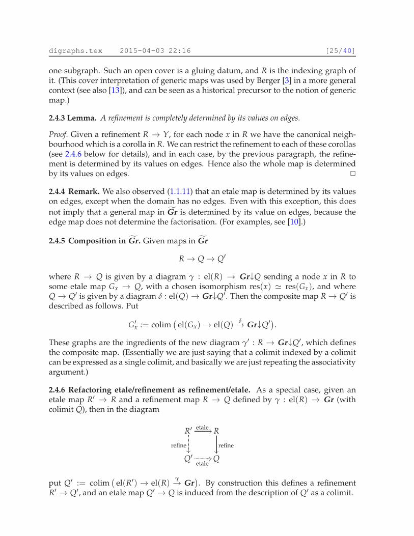
2.4.6 Refactoring etale/refinement as refinement/etale. As a special case, given anetale map R′ → R and a refinement map R → Q defined by γ : el(R) → Gr (withcolimit Q), then in the diagram

R′etale //

refine��

R

refine��

Q′etale

// Q

put Q′ := colim(

el(R′) → el(R)γ→ Gr

). By construction this defines a refinement

R′ → Q′, and an etale map Q′ → Q is induced from the description of Q′ as a colimit.

digraphs.tex 2015-04-03 22:16 [26/40]

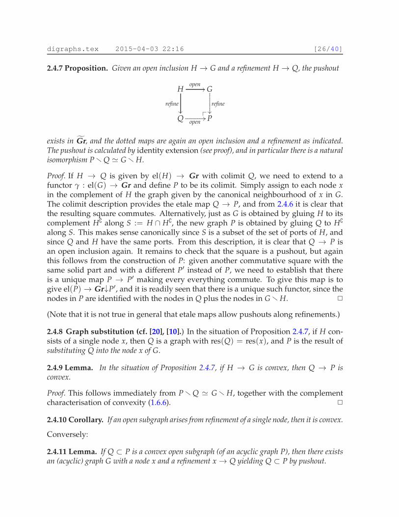
2.4.7 Proposition. Given an open inclusion H → G and a refinement H → Q, the pushout

Hopen

//

refine

��

G

refine

��

Q open// P❴✤

exists in G̃r, and the dotted maps are again an open inclusion and a refinement as indicated.The pushout is calculated by identity extension (see proof), and in particular there is a naturalisomorphism PrQ ≃ Gr H.

Proof. If H → Q is given by el(H) → Gr with colimit Q, we need to extend to afunctor γ : el(G) → Gr and define P to be its colimit. Simply assign to each node xin the complement of H the graph given by the canonical neighbourhood of x in G.The colimit description provides the etale map Q → P, and from 2.4.6 it is clear thatthe resulting square commutes. Alternatively, just as G is obtained by gluing H to itscomplement H∁ along S := H ∩ H∁, the new graph P is obtained by gluing Q to H∁

along S. This makes sense canonically since S is a subset of the set of ports of H, andsince Q and H have the same ports. From this description, it is clear that Q → P isan open inclusion again. It remains to check that the square is a pushout, but againthis follows from the construction of P: given another commutative square with thesame solid part and with a different P′ instead of P, we need to establish that thereis a unique map P → P′ making every everything commute. To give this map is togive el(P) → Gr↓P′, and it is readily seen that there is a unique such functor, since thenodes in P are identified with the nodes in Q plus the nodes in Gr H. ✷

(Note that it is not true in general that etale maps allow pushouts along refinements.)

2.4.8 Graph substitution (cf. [20], [10].) In the situation of Proposition 2.4.7, if H con-sists of a single node x, then Q is a graph with res(Q) = res(x), and P is the result ofsubstituting Q into the node x of G.

2.4.9 Lemma. In the situation of Proposition 2.4.7, if H → G is convex, then Q → P isconvex.

Proof. This follows immediately from Pr Q ≃ Gr H, together with the complementcharacterisation of convexity (1.6.6). ✷

2.4.10 Corollary. If an open subgraph arises from refinement of a single node, then it is convex.

Conversely:

2.4.11 Lemma. If Q ⊂ P is a convex open subgraph (of an acyclic graph P), then there existsan (acyclic) graph G with a node x and a refinement x → Q yielding Q ⊂ P by pushout.

digraphs.tex 2015-04-03 22:16 [27/40]

Proof. If G and x exist, we must have Gr x = PrQ. Put S := Q ∩ Q∁, then P is thegluing

S ⇒ Q + Q∁ → P.

Since S ⊂ ports(Q) = ports(res Q), we can glue in res(Q) instead of Q, obtaining G inthis way:

S ⇒ res(Q) + Q∁ → G.

It remains to see that G is acyclic — this is where convexity of Q comes in: a wheel inG through x would induce a path in Gr x = Pr Q from an edge in S to another edgein S. But this is impossible since Q is convex (1.6.6). (And of course G cannot contain awheel not through x, since they would also be a wheel in Gr x = PrQ ⊂ P.) ✷

(Note that G might be an inner edge in Y; then the complement is not a subgraph.)

Corollary 2.4.10 and Lemma 2.4.11 together are also established in [10], Theorem5.38, modulo set-up and terminology.

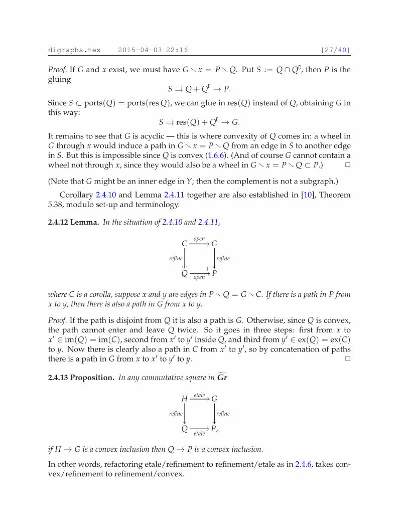
2.4.12 Lemma. In the situation of 2.4.10 and 2.4.11,

Copen

//

refine

��

G

refine

��

Qopen

// P❴✤

where C is a corolla, suppose x and y are edges in PrQ = GrC. If there is a path in P fromx to y, then there is also a path in G from x to y.

Proof. If the path is disjoint from Q it is also a path is G. Otherwise, since Q is convex,the path cannot enter and leave Q twice. So it goes in three steps: first from x tox′ ∈ im(Q) = im(C), second from x′ to y′ inside Q, and third from y′ ∈ ex(Q) = ex(C)to y. Now there is clearly also a path in C from x′ to y′, so by concatenation of pathsthere is a path in G from x to x′ to y′ to y. ✷

2.4.13 Proposition. In any commutative square in G̃r

Hetale //

refine

��

G

refine

��

Qetale

// P,

if H → G is a convex inclusion then Q→ P is a convex inclusion.

In other words, refactoring etale/refinement to refinement/etale as in 2.4.6, takes con-vex/refinement to refinement/convex.

digraphs.tex 2015-04-03 22:16 [28/40]

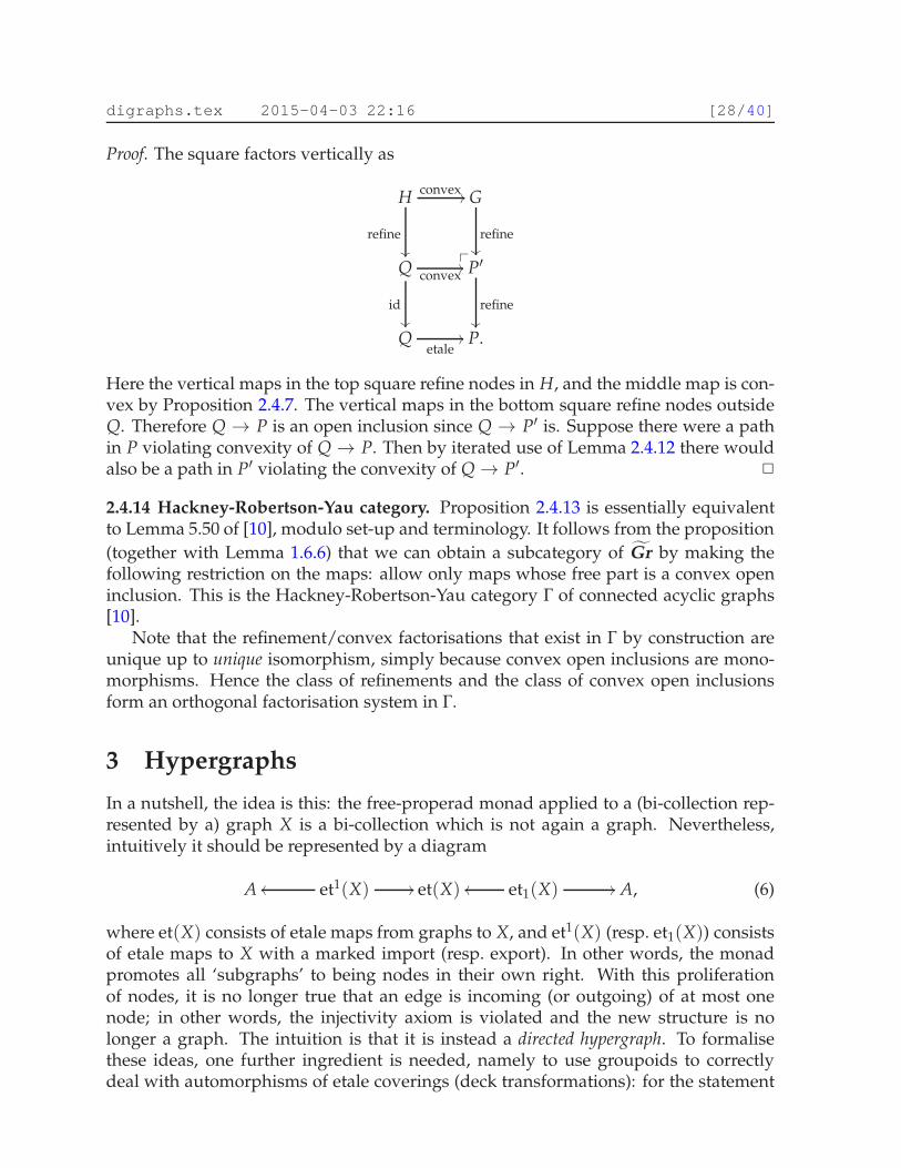
Proof. The square factors vertically as

Hconvex //

refine��

G

refine��

Q convex//

id��

P′❴✤

refine��

Qetale

// P.

Here the vertical maps in the top square refine nodes in H, and the middle map is con-vex by Proposition 2.4.7. The vertical maps in the bottom square refine nodes outsideQ. Therefore Q → P is an open inclusion since Q → P′ is. Suppose there were a pathin P violating convexity of Q → P. Then by iterated use of Lemma 2.4.12 there wouldalso be a path in P′ violating the convexity of Q→ P′. ✷

2.4.14 Hackney-Robertson-Yau category. Proposition 2.4.13 is essentially equivalentto Lemma 5.50 of [10], modulo set-up and terminology. It follows from the proposition(together with Lemma 1.6.6) that we can obtain a subcategory of G̃r by making thefollowing restriction on the maps: allow only maps whose free part is a convex openinclusion. This is the Hackney-Robertson-Yau category Γ of connected acyclic graphs[10].

Note that the refinement/convex factorisations that exist in Γ by construction areunique up to unique isomorphism, simply because convex open inclusions are mono-morphisms. Hence the class of refinements and the class of convex open inclusionsform an orthogonal factorisation system in Γ.

3 Hypergraphs

In a nutshell, the idea is this: the free-properad monad applied to a (bi-collection rep-resented by a) graph X is a bi-collection which is not again a graph. Nevertheless,intuitively it should be represented by a diagram

A et1(X)oo // et(X) et1(X)oo // A, (6)

where et(X) consists of etale maps from graphs to X, and et1(X) (resp. et1(X)) consistsof etale maps to X with a marked import (resp. export). In other words, the monadpromotes all ‘subgraphs’ to being nodes in their own right. With this proliferationof nodes, it is no longer true that an edge is incoming (or outgoing) of at most onenode; in other words, the injectivity axiom is violated and the new structure is nolonger a graph. The intuition is that it is instead a directed hypergraph. To formalisethese ideas, one further ingredient is needed, namely to use groupoids to correctlydeal with automorphisms of etale coverings (deck transformations): for the statement

digraphs.tex 2015-04-03 22:16 [29/40]

to be correct we must use groupoid-enriched hypergraphs. Specifically, we need et(X) tobe the groupoid of all etale maps to X, not just the set of iso-classes of such.

The main result of this section, Theorem 3.4.5, states that the free properad on a hyper-graph is again a hypergraph (given by (6)).

3.1 Discrete hypergraphs

The theory of hypergraphs is a extensive research topic, with a variety of differentapplications in computer science. A standard text book on hypergraphs is Berge [2].For the notion of directed hypergraph, a classical reference is [5]. Here we take a novelapproach to directed hypergraphs, englobing naturally the theory of directed graphsabove.

3.1.1 Directed hypergraphs. A directed hypergraph is a diagram of sets

A Isoop

// N Oq

oo t // A

for which both I → A × N and O → N × A are relations (i.e. are injective maps).The elements in N are called nodes; the elements in A are called hyperedges. A hyper-edge connects one set of nodes to another set of nodes. A directed hypergraph can berepresented by two incidence matrices between nodes and hyperedges. A directed hy-pergraph is called loopfree if these two relations are disjoint, i.e. if also I + O → A× Nis a relation. (This simply means that a hyperedge cannot contain the same node in itsdomain and in its codomain.) Loopfree hypergraphs are what are called hypergraphsin [5], where they are encoded as a single signed incidence matrix. For the presentpurposes it is essential to allow loops.

From now on we simply say hypergraph for directed hypergraph.A graph is a hypergraph, since a diagram (1) clearly satisfies the conditions: if s and

t are themselves injective, clearly the two spans are relations. For the present purposes,a fruitful interpretation of the hypergraph axiom, is that a hypergraph is locally a graph,in the sense that for each node x, the maps Ix → A and Ox → A are injective. In factconversely, if for every node x the maps Ix → A and Ox → A are injective then X is ahypergraph. Indeed, I = ∑x∈N Ix and A× N = ∑x∈N A, and the map I → A× N isjust the sum of all the maps Ix → A. Similarly for O.

The notion of hypergraph has a self-duality, in the sense that interchanging therole of nodes and hyperedges yields again a hypergraph. However, the study of hy-pergraphs is biased, so that all notions are geared towards the embedding of graphsinherent in the choice of symbols. With the asymmetry in mind, we define classes ofmorphisms as follows. A morphism is a diagram like (2); it is etale if the middle squaresare pullbacks, and an open inclusion if it is level-wise injective and etale. (Note that ac-cording to this definition, etale maps are arity-preserving for nodes, but not necessarilyon hyperedges.)

Observe that we have not required the sets to be finite. This is because the freeproperad on a graph may be an infinite hypergraph (just as the free category on a

digraphs.tex 2015-04-03 22:16 [30/40]

(closed) directed graph may be an infinite category). The relevant finiteness conditionis just that p and q be finite maps. These are called hypergraphs of finite type. Hence-forth we only consider hypergraphs of finite type.

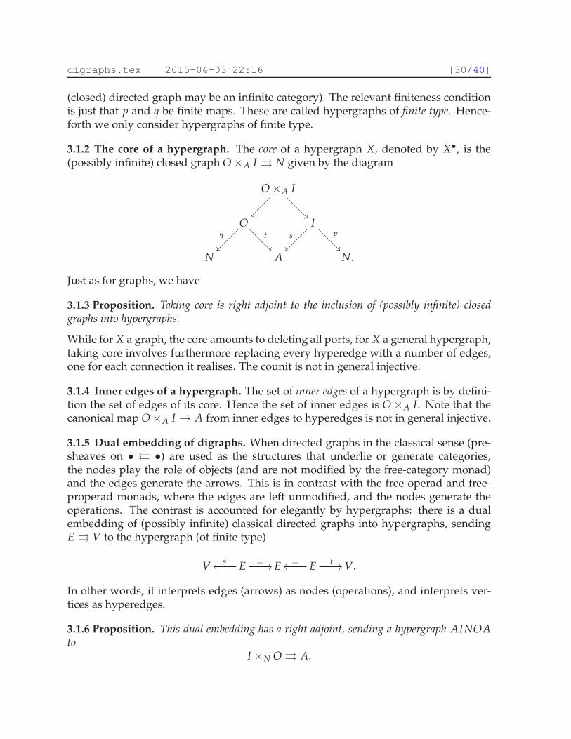
3.1.2 The core of a hypergraph. The core of a hypergraph X, denoted by X•, is the(possibly infinite) closed graph O×A I ⇒ N given by the diagram

O×A I

��⑧⑧⑧⑧⑧⑧

��❄❄❄

❄❄❄❄

Oq

��⑧⑧⑧⑧⑧⑧⑧

t

��❄❄❄

❄❄❄❄

Is

��⑧⑧⑧⑧⑧⑧⑧ p

��❄❄❄

❄❄❄❄

N A N.

Just as for graphs, we have

3.1.3 Proposition. Taking core is right adjoint to the inclusion of (possibly infinite) closedgraphs into hypergraphs.

While for X a graph, the core amounts to deleting all ports, for X a general hypergraph,taking core involves furthermore replacing every hyperedge with a number of edges,one for each connection it realises. The counit is not in general injective.

3.1.4 Inner edges of a hypergraph. The set of inner edges of a hypergraph is by defini-tion the set of edges of its core. Hence the set of inner edges is O×A I. Note that thecanonical map O×A I → A from inner edges to hyperedges is not in general injective.

3.1.5 Dual embedding of digraphs. When directed graphs in the classical sense (pre-sheaves on • ⇔ •) are used as the structures that underlie or generate categories,the nodes play the role of objects (and are not modified by the free-category monad)and the edges generate the arrows. This is in contrast with the free-operad and free-properad monads, where the edges are left unmodified, and the nodes generate theoperations. The contrast is accounted for elegantly by hypergraphs: there is a dualembedding of (possibly infinite) classical directed graphs into hypergraphs, sendingE ⇒ V to the hypergraph (of finite type)

V Esoo = // E E=oo t // V.

In other words, it interprets edges (arrows) as nodes (operations), and interprets ver-tices as hyperedges.

3.1.6 Proposition. This dual embedding has a right adjoint, sending a hypergraph AINOAto

I ×N O ⇒ A.

digraphs.tex 2015-04-03 22:16 [31/40]

3.1.7 Sums, connectedness, acyclicity, loops. The notions of connectedness and acyclic-ity are defined in the same way for hypergraphs as for graphs, but do not play an im-portant role for the present purposes, as the free properad on a connected acyclic graphis a hypergraph which may be neither connected nor acyclic. (Specifically, if a graph Xhas no ports, then X will contain a corresponding isolated node, while each edge in agraph X will become a node in X with that same edge as a loop.)

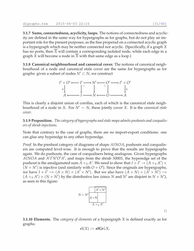
3.1.8 Canonical neighbourhood and canonical cover. The notions of canonical neigh-bourhood of a node and canonical etale cover are the same for hypergraphs as forgraphs: given a subset of nodes N′ ⊂ N, we construct

I ′ + O′

�

I ′oo

��

❴✤

// N′

��

O′oo✤❴

��

// I ′ + O′

�

A Ioo // N Ooo // A

This is clearly a disjoint union of corollas, each of which is the canonical etale neigh-bourhood of a node in X. For N′ = N, these jointly cover X. It is the canonical etalecover.

3.1.9 Proposition. The category of hypergraphs and etale maps admits pushouts and coequalis-ers of shrub injections.

Note that contrary to the case of graphs, there are no import-export conditions: onecan glue any hyperedge to any other hyperedge.

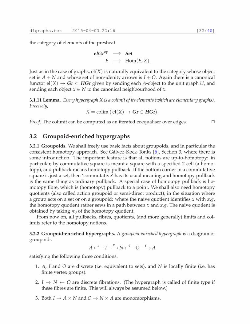
Proof. In the presheaf category of diagrams of shape AINOA, pushouts and coequalis-ers are computed level-wise. It is enough to prove that the results are hypergraphsagain. We do pushouts, the case of coequalisers being analogous. Given hypergraphsAINOA and A′ I ′N′O′A′, and maps from the shrub S000S, the hyperedge set of thepushout is the amalgamated sum A +S A′. We need to show that I + I ′ → (A +S A′)×(N + N′) is injective (and similarly with O + O′). Since the originals are hypergraphs,we have I + I ′ →֒ (A × N) + (A′ × N′). But we also have (A × N) + (A′ × N′) →֒(A +S A′)× (N + N′) by the distributive law (since N and N′ are disjoint in N + N′),as seen in this figure:

A×N

A′×N′

A +S A′

N + N′

✷

3.1.10 Elements. The category of elements of a hypergraph X is defined exactly as forgraphs:

el(X) := elGr↓X,

digraphs.tex 2015-04-03 22:16 [32/40]

the category of elements of the presheaf

elGrop −→ Set

E 7−→ Hom(E, X).

Just as in the case of graphs, el(X) is naturally equivalent to the category whose objectset is A + N and whose set of non-idenity arrows is I + O. Again there is a canonicalfunctor el(X) → Gr ⊂ HGr given by sending each A-object to the unit graph U, andsending each object x ∈ N to the canonical neighbourhood of x.

3.1.11 Lemma. Every hypergraph X is a colimit of its elements (which are elementary graphs).Precisely,

X = colim(

el(X) → Gr ⊂ HGr).

Proof. The colimit can be computed as an iterated coequaliser over edges. ✷

3.2 Groupoid-enriched hypergraphs

3.2.1 Groupoids. We shall freely use basic facts about groupoids, and in particular theconsistent homotopy approach. See Gálvez-Kock-Tonks [6], Section 3, where there issome introduction. The important feature is that all notions are up-to-homotopy: inparticular, by commutative square is meant a square with a specified 2-cell (a homo-topy), and pullback means homotopy pullback. If the bottom corner in a commutativesquare is just a set, then ‘commutative’ has its usual meaning and homotopy pullbackis the same thing as ordinary pullback. A special case of homotopy pullback is ho-motopy fibre, which is (homotopy) pullback to a point. We shall also need homotopyquotients (also called action groupoid or semi-direct product), in the situation wherea group acts on a set or on a groupoid: where the naive quotient identifies x with x.g,the homotopy quotient rather sews in a path between x and x.g. The naive quotient isobtained by taking π0 of the homotopy quotient.

From now on, all pullbacks, fibres, quotients, (and more generally) limits and col-imits refer to the homotopy notions.

3.2.2 Groupoid-enriched hypergraphs. A groupoid-enriched hypergraph is a diagram ofgroupoids

A Isoop

// N Oq

oo t // A

satisfying the following three conditions.

1. A, I and O are discrete (i.e. equivalent to sets), and N is locally finite (i.e. hasfinite vertex groups).

2. I → N ← O are discrete fibrations. (The hypergraph is called of finite type ifthese fibres are finite. This will always be assumed below.)

3. Both I → A× N and O→ N × A are monomorphisms.

digraphs.tex 2015-04-03 22:16 [33/40]

Observe that from condition 1 and 2 we have the diagram

I

��

discr.fib

##●●●

●●●●

●●●

A× Ndiscr.fib

// N

and therefore also I → A × N is automatically a discrete fibration, i.e. has discrete(homotopy) fibres. Condition 3 says that these discrete fibres are either singleton orempty.

Observe that since I (resp. O) is discrete, and also the fibres Ix (resp. Ox) are discrete,the map I → N (resp. O → N) is in fact a disjoint union of torsors. More precisely, foreach x ∈ N, the vertex group AutN(x) acts freely on Ix (resp. on Ox). This means thatlocally at each node x, the hypergraph is a ‘stacky corolla’, as detailed below.

3.2.3 Etale maps. An etale map of groupoid-enriched hypergraphs is a diagram

A′

�

I ′oo

❴✤

��

// N′

��

O′oo✤❴

��

// A′

�

A Ioo // N Ooo // A

in which the middle squares are (homotopy) pullbacks. We denote by HGr the cate-gory of (groupoid-enriched, finite-type) hypergraphs and etale maps.

3.2.4 Stacky corollas. Consider a corolla Cmn :

m + n← m→ 1← n→ m + n

and suppose that a finite group G acts freely on m and freely on n. Then we can formthe levelwise homotopy quotient, which receives an etale map from Cm

n :

m + n

��

moo

❴✤

//

��

1

��

noo✤❴

��

// m + n

��m+n

GmG

oo // 1G

nG

oo // m+nG

The result is a hypergraph Cmn /G called a stacky corolla. It arises as the homotopy

coequaliserCm

n × G ⇒ Cmn → Cm

n /G,

where G denotes the discrete set of elements in the group G, and Cmn × G denotes the

disjoint union of that many copies of Cmn .

3.2.5 Hypergraphs as colimits of elementary graphs. We need the groupoid versionof the result that every hypergraph X is the colimit of its elements. This is true again:the category of elements elGr↓X can be described explicitly as having object set A +

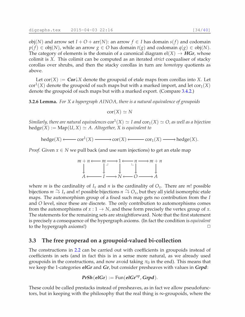
digraphs.tex 2015-04-03 22:16 [34/40]

obj(N) and arrow set I + O + arr(N): an arrow f ∈ I has domain s( f ) and codomainp( f ) ∈ obj(N), while an arrow g ∈ O has domain t(g) and codomain q(g) ∈ obj(N).The category of elements is the domain of a canonical diagram el(X) → HGr, whosecolimit is X. This colimit can be computed as an iterated strict coequaliser of stackycorollas over shrubs, and then the stacky corollas in turn are homotopy quotients asabove.

Let cor(X) := Cor↓X denote the groupoid of etale maps from corollas into X. Letcor1(X) denote the groupoid of such maps but with a marked import, and let cor1(X)denote the groupoid of such maps but with a marked export. (Compare 3.4.2.)

3.2.6 Lemma. For X a hypergraph AINOA, there is a natural equivalence of groupoids

cor(X) ≃ N

Similarly, there are natural equivalences cor1(X) ≃ I and cor1(X) ≃ O, as well as a bijectionhedge(X) := Map(U, X) ≃ A. Altogether, X is equivalent to

hedge(X) cor1(X)oo // cor(X) cor1(X)oo // hedge(X).

Proof. Given x ∈ N we pull back (and use sum injections) to get an etale map

m + n

��

moo

❴✤

//

��

1

��

noo✤❴

��

// m + n

��

A Ioo // N Ooo // A

where m is the cardinality of Ix and n is the cardinality of Ox. There are m! possiblebijections m ∼→ Ix and n! possible bijections n ∼→ Ox, but they all yield isomorphic etalemaps. The automorphism group of a fixed such map gets no contribution from the Iand O level, since these are discrete. The only contribution to automorphisms comesfrom the automorphisms of x : 1→ N, and these form precisely the vertex group of x.The statements for the remaining sets are straightforward. Note that the first statementis precisely a consequence of the hypergraph axioms. (In fact the condition is equivalentto the hypergraph axioms!) ✷

3.3 The free properad on a groupoid-valued bi-collection

The constructions in 2.2 can be carried out with coefficients in groupoids instead ofcoefficients in sets (and in fact this is in a sense more natural, as we already usedgroupoids in the constructions, and now avoid taking π0 in the end). This means thatwe keep the 1-categories elGr and Gr, but consider presheaves with values in Grpd :

PrSh (elGr) := Fun(elGrop, Grpd ).

These could be called prestacks instead of presheaves, as in fact we allow pseudofunc-tors, but in keeping with the philosophy that the real thing is ∞-groupoids, where the

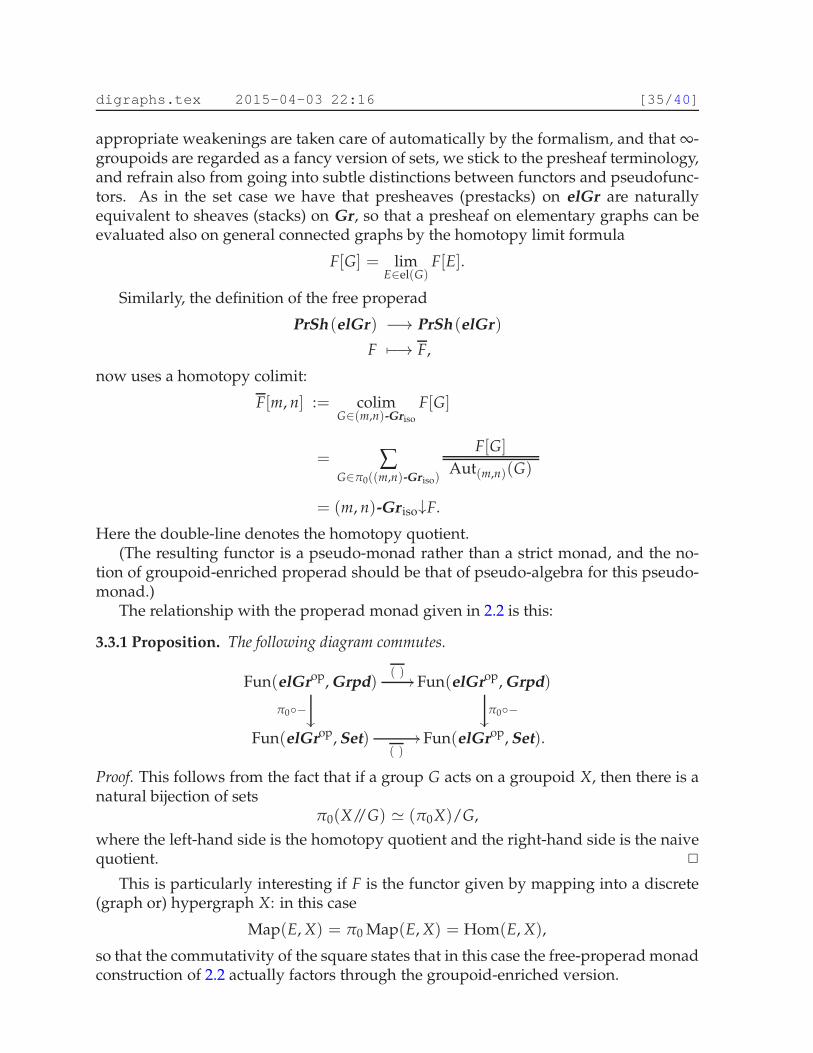
digraphs.tex 2015-04-03 22:16 [35/40]

appropriate weakenings are taken care of automatically by the formalism, and that ∞-groupoids are regarded as a fancy version of sets, we stick to the presheaf terminology,and refrain also from going into subtle distinctions between functors and pseudofunc-tors. As in the set case we have that presheaves (prestacks) on elGr are naturallyequivalent to sheaves (stacks) on Gr, so that a presheaf on elementary graphs can beevaluated also on general connected graphs by the homotopy limit formula

F[G] = limE∈el(G)

F[E].

Similarly, the definition of the free properad

PrSh (elGr) −→ PrSh (elGr)

F 7−→ F,

now uses a homotopy colimit:

F[m, n] := colimG∈(m,n)-Griso

F[G]

= ∑G∈π0((m,n)-Gr iso)

F[G]

Aut(m,n)(G)

= (m, n)-Gr iso↓F.

Here the double-line denotes the homotopy quotient.(The resulting functor is a pseudo-monad rather than a strict monad, and the no-

tion of groupoid-enriched properad should be that of pseudo-algebra for this pseudo-monad.)

The relationship with the properad monad given in 2.2 is this:

3.3.1 Proposition. The following diagram commutes.

Fun(elGrop, Grpd)( )

//

π0◦−��

Fun(elGrop, Grpd)

π0◦−��

Fun(elGrop, Set)( )

// Fun(elGrop, Set).

Proof. This follows from the fact that if a group G acts on a groupoid X, then there is anatural bijection of sets

π0(X//G) ≃ (π0X)/G,

where the left-hand side is the homotopy quotient and the right-hand side is the naivequotient. ✷

This is particularly interesting if F is the functor given by mapping into a discrete(graph or) hypergraph X: in this case

Map(E, X) = π0 Map(E, X) = Hom(E, X),

so that the commutativity of the square states that in this case the free-properad monadconstruction of 2.2 actually factors through the groupoid-enriched version.

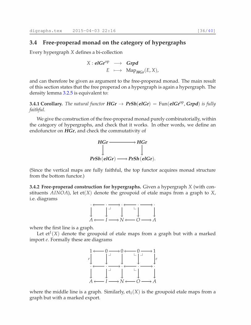
digraphs.tex 2015-04-03 22:16 [36/40]

3.4 Free-properad monad on the category of hypergraphs

Every hypergraph X defines a bi-collection

X : elGrop −→ Grpd

E 7−→ MapHGr(E, X),

and can therefore be given as argument to the free-properad monad. The main resultof this section states that the free properad on a hypergraph is again a hypergraph. Thedensity lemma 3.2.5 is equivalent to:

3.4.1 Corollary. The natural functor HGr → PrSh(elGr) = Fun(elGrop, Grpd) is fullyfaithful.

We give the construction of the free-properad monad purely combinatorially, withinthe category of hypergraphs, and check that it works. In other words, we define anendofunctor on HGr, and check the commutativity of

HGr //

��

HGr

��

PrSh (elGr) // PrSh (elGr).

(Since the vertical maps are fully faithful, the top functor acquires monad structurefrom the bottom functor.)

3.4.2 Free-properad construction for hypergraphs. Given a hypergraph X (with con-stituents AINOA), let et(X) denote the groupoid of etale maps from a graph to X,i.e. diagrams

·

��

·oo

��

//

❴✤ ·

��

·✤❴

oo

��

// ·

��

A Ioo // N Ooo // A

where the first line is a graph.Let et1(X) denote the groupoid of etale maps from a graph but with a marked

import e. Formally these are diagrams

1e��

0oo

��

❴✤

// 0

��

0✤❴ ❴

✤oo

��

// 1e��

·

��

·oo

��

//

❴✤ ·

��

·✤❴

oo

��

// ·

��

A Ioo // N Ooo // A

where the middle line is a graph. Similarly, et1(X) is the groupoid etale maps from agraph but with a marked export.

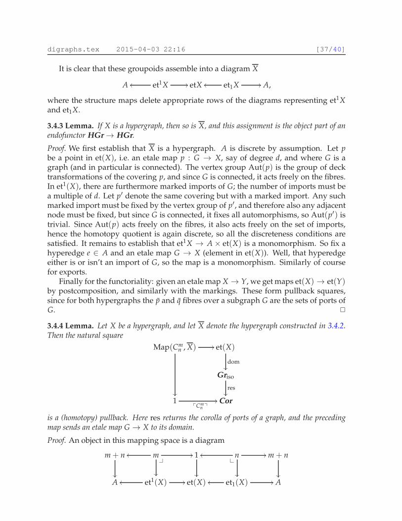
digraphs.tex 2015-04-03 22:16 [37/40]

It is clear that these groupoids assemble into a diagram X

A et1Xoo // etX et1Xoo // A,

where the structure maps delete appropriate rows of the diagrams representing et1Xand et1X.

3.4.3 Lemma. If X is a hypergraph, then so is X, and this assignment is the object part of anendofunctor HGr→ HGr.

Proof. We first establish that X is a hypergraph. A is discrete by assumption. Let pbe a point in et(X), i.e. an etale map p : G → X, say of degree d, and where G is agraph (and in particular is connected). The vertex group Aut(p) is the group of decktransformations of the covering p, and since G is connected, it acts freely on the fibres.In et1(X), there are furthermore marked imports of G; the number of imports must bea multiple of d. Let p′ denote the same covering but with a marked import. Any suchmarked import must be fixed by the vertex group of p′, and therefore also any adjacentnode must be fixed, but since G is connected, it fixes all automorphisms, so Aut(p′) istrivial. Since Aut(p) acts freely on the fibres, it also acts freely on the set of imports,hence the homotopy quotient is again discrete, so all the discreteness conditions aresatisfied. It remains to establish that et1X → A× et(X) is a monomorphism. So fix ahyperedge e ∈ A and an etale map G → X (element in et(X)). Well, that hyperedgeeither is or isn’t an import of G, so the map is a monomorphism. Similarly of coursefor exports.

Finally for the functoriality: given an etale map X → Y, we get maps et(X) → et(Y)by postcomposition, and similarly with the markings. These form pullback squares,since for both hypergraphs the p̄ and q̄ fibres over a subgraph G are the sets of ports ofG. ✷

3.4.4 Lemma. Let X be a hypergraph, and let X denote the hypergraph constructed in 3.4.2.Then the natural square

Map(Cmn , X) //

��

et(X)

dom��

Griso

res��

1pCm

n q// Cor

is a (homotopy) pullback. Here res returns the corolla of ports of a graph, and the precedingmap sends an etale map G→ X to its domain.

Proof. An object in this mapping space is a diagram

m + n

��

moo

❴✤

//

��

1

��

noo✤❴

��

// m + n

��

A et1(X)oo // et(X) et1(X)oo // A

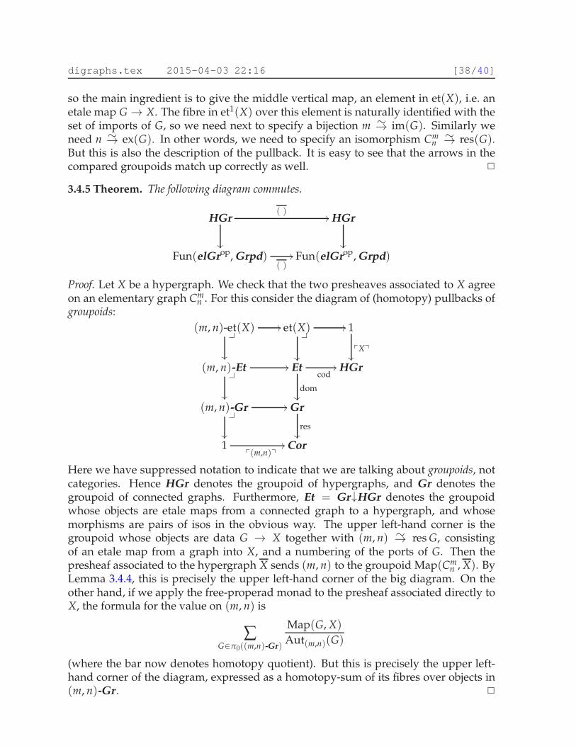
digraphs.tex 2015-04-03 22:16 [38/40]

so the main ingredient is to give the middle vertical map, an element in et(X), i.e. anetale map G→ X. The fibre in et1(X) over this element is naturally identified with theset of imports of G, so we need next to specify a bijection m ∼→ im(G). Similarly weneed n ∼→ ex(G). In other words, we need to specify an isomorphism Cm

n∼→ res(G).

But this is also the description of the pullback. It is easy to see that the arrows in thecompared groupoids match up correctly as well. ✷

3.4.5 Theorem. The following diagram commutes.

HGr( )

//

��

HGr

��

Fun(elGrop, Grpd)( )

// Fun(elGrop, Grpd)

Proof. Let X be a hypergraph. We check that the two presheaves associated to X agreeon an elementary graph Cm

n . For this consider the diagram of (homotopy) pullbacks ofgroupoids:

(m, n)-et(X)❴✤

//

��

et(X)❴✤

��

// 1

pXq��

(m, n)-Et❴✤

��

// Et

dom��

cod// HGr

(m, n)-Gr❴✤

��

// Gr

res��

1p(m,n)q

// Cor

Here we have suppressed notation to indicate that we are talking about groupoids, notcategories. Hence HGr denotes the groupoid of hypergraphs, and Gr denotes thegroupoid of connected graphs. Furthermore, Et = Gr↓HGr denotes the groupoidwhose objects are etale maps from a connected graph to a hypergraph, and whosemorphisms are pairs of isos in the obvious way. The upper left-hand corner is thegroupoid whose objects are data G → X together with (m, n) ∼→ res G, consistingof an etale map from a graph into X, and a numbering of the ports of G. Then thepresheaf associated to the hypergraph X sends (m, n) to the groupoid Map(Cm

n , X). ByLemma 3.4.4, this is precisely the upper left-hand corner of the big diagram. On theother hand, if we apply the free-properad monad to the presheaf associated directly toX, the formula for the value on (m, n) is

∑G∈π0((m,n)-Gr)

Map(G, X)

Aut(m,n)(G)

(where the bar now denotes homotopy quotient). But this is precisely the upper left-hand corner of the diagram, expressed as a homotopy-sum of its fibres over objects in(m, n)-Gr . ✷

digraphs.tex 2015-04-03 22:16 [39/40]

3.4.6 Remark. Under the ‘dual embedding’ of (closed) directed graphs into hyper-graphs 3.1.5, the free-properad monad restricts to the free-category monad. (In thiscase, the groupoids involved are discrete.)

References

[1] MICHAEL BATANIN and CLEMENS BERGER. Homotopy theory for algebras over polynomialmonads. Preprint, arXiv:1305.0086.

[2] CLAUDE BERGE. Hypergraphs, vol. 45 of North-Holland Mathematical Library. North-Holland Publishing Co., Amsterdam, 1989.

[3] CLEMENS BERGER. A cellular nerve for higher categories. Adv. Math. 169 (2002), 118–175.

[4] CLEMENS BERGER, PAUL-ANDRÉ MELLIÈS, and MARK WEBER. Monads with arities andtheir associated theories. J. Pure Appl. Algebra 216 (2012), 2029–2048. ArXiv:1101.3064.

[5] GIORGIO GALLO, GIUSTINO LONGO, STEFANO PALLOTTINO, and SANG NGUYEN.Directed hypergraphs and applications. Discrete Appl. Math. 42 (1993), 177–201.

[6] IMMA GÁLVEZ-CARRILLO, JOACHIM KOCK, and ANDREW TONKS. Groupoids and Faàdi Bruno formulae for Green functions in bialgebras of trees. Adv. Math. 254 (2014), 79–117.ArXiv:1207.6404.

[7] WEE LIANG GAN. Koszul duality for dioperads. Math. Res. Lett. 10 (2003), 109–124.ArXiv:math/0201074.

[8] DAVID GEPNER and JOACHIM KOCK. Polynomial functors over infinity categories. In prepa-ration.

[9] EZRA GETZLER and MIKHAIL M. KAPRANOV. Modular operads. Compositio Math. 110

(1998), 65–126.

[10] PHILIP HACKNEY, MARCY ROBERTSON, and DONALD YAU. Infinity Properads and InfinityWheeled Properads. To appear in Springer Lecture Notes in Mathematics. ArXiv:1410.6716.

[11] ANDRÉ JOYAL and JOACHIM KOCK. Feynman graphs, and nerve theorem for compact sym-metric multicategories (extended abstract). In Proceedings of the 6th International Workshop onQuantum Physics and Logic (Oxford 2009), vol. 270 of Electronic Notes in Theoretical Com-puter Science, pp. 105–113, 2011. ArXiv:0908.2675.

[12] ANDRÉ JOYAL and IEKE MOERDIJK. A completeness theorem for open maps. Ann. Pure Appl.Logic 70 (1994), 51–86.

[13] JOACHIM KOCK. Polynomial functors and trees. Internat. Math. Res. Notices 2011 (2011),609–673. ArXiv:0807.2874.

[14] JOACHIM KOCK. Data types with symmetries and polynomial functors over groupoids. In Pro-ceedings of the 28th Conference on the Mathematical Foundations of Programming Semantics(Bath, 2012), vol. 286 of Electronic Notes in Theoretical Computer Science, pages 351–365,2012. Arxiv:1210.0828.

digraphs.tex 2015-04-03 22:16 [40/40]

[15] SAUNDERS MAC LANE. Categories for the working mathematician, second edition. No. 5 inGraduate Texts in Mathematics. Springer-Verlag, New York, 1998.

[16] MANFRED E. SZABO. Polycategories. Comm. Algebra 3 (1975), 663–689.

[17] BRUNO VALLETTE. A Koszul duality for PROPs. Trans. Amer. Math. Soc. 359 (2007), 4865–4943. ArXiv:math/0411542.

[18] MARK WEBER. Generic morphisms, parametric representations and weakly Cartesian monads.Theory Appl. Categ. 13 (2004), 191–234 (electronic).

[19] MARK WEBER. Familial 2-functors and parametric right adjoints. Theory Appl. Categ. 18

(2007), 665–732 (electronic).

[20] DONALD YAU and MARK W. JOHNSON. A Foundation for PROPs, Algebras, and Mod-ules. Vol. 203 of Mathematical Surveys and Monographs, American Mathematical Society,Providence, RI.