1

2

3

4

5

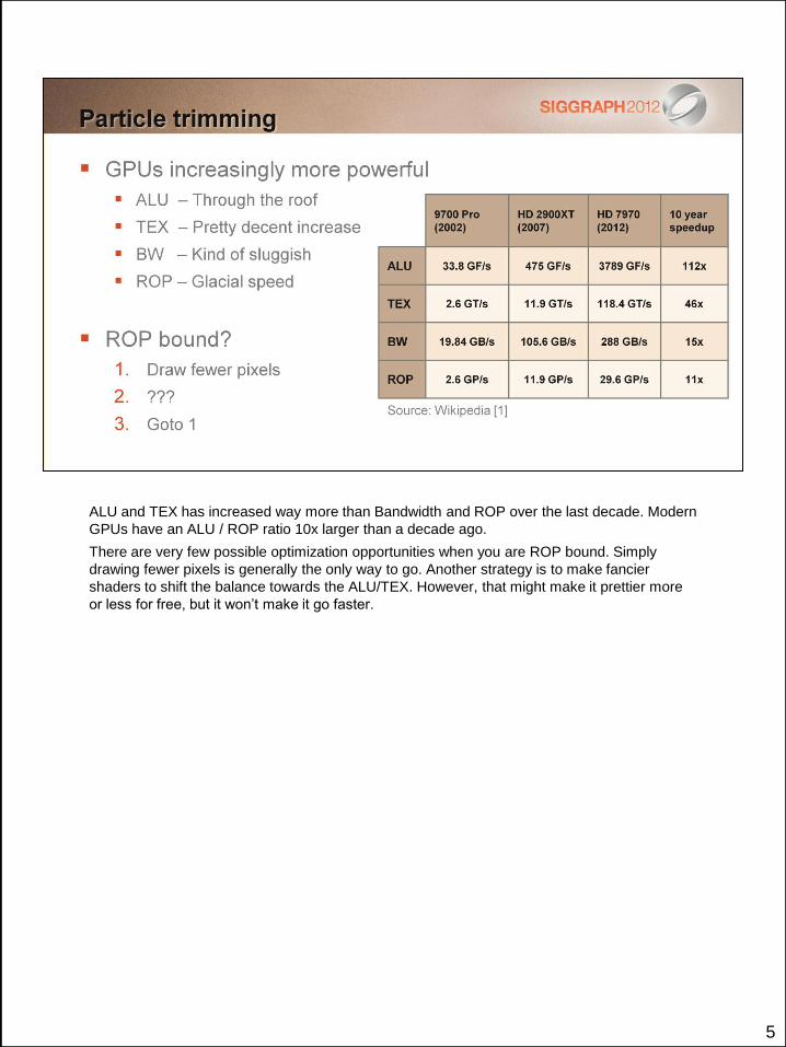
ALU and TEX has increased way more than Bandwidth and ROP over the last decade. Modern

GPUs have an ALU / ROP ratio 10x larger than a decade ago.

There are very few possible optimization opportunities when you are ROP bound. Simply

drawing fewer pixels is generally the only way to go. Another strategy is to make fancier

shaders to shift the balance towards the ALU/TEX. However, that might make it prettier more

or less for free, but it won’t make it go faster.

6

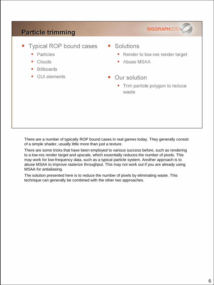
There are a number of typically ROP bound cases in real games today. They generally consist

of a simple shader, usually little more than just a texture.

There are some tricks that have been employed to various success before, such as rendering

to a low-res render target and upscale, which essentially reduces the number of pixels. This

may work for low-frequency data, such as a typical particle system. Another approach is to

abuse MSAA to improve rasterize throughput. This may not work out if you are already using

MSAA for antialiasing.

The solution presented here is to reduce the number of pixels by eliminating waste. This

technique can generally be combined with the other two approaches.

7

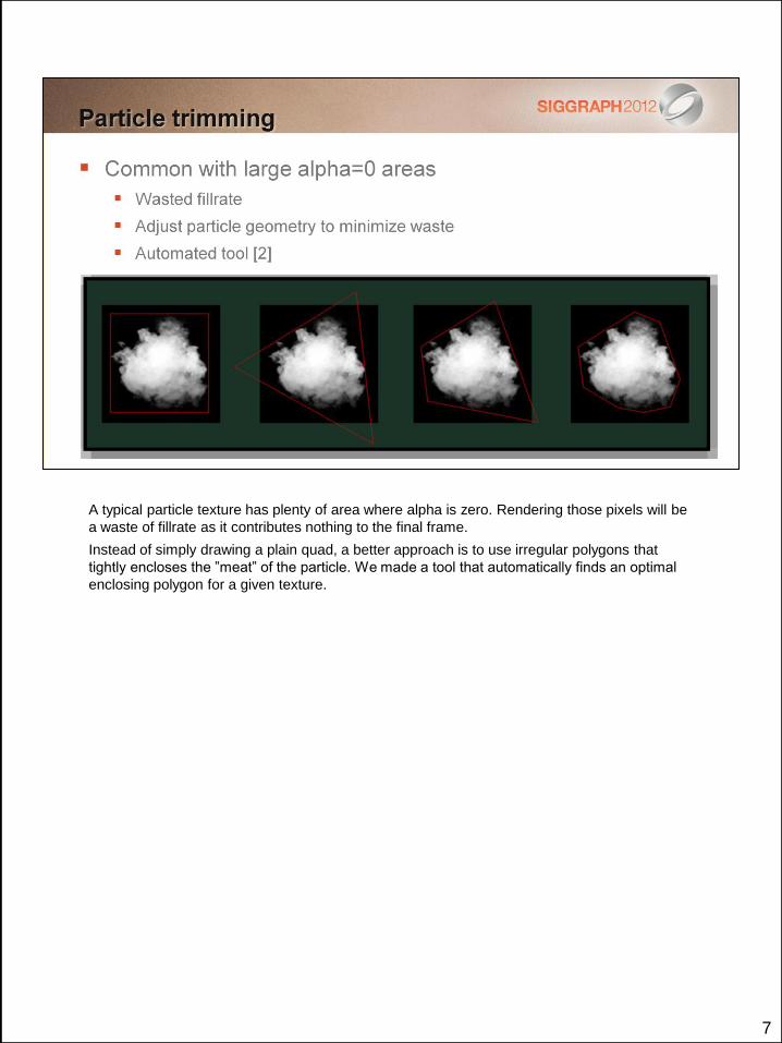
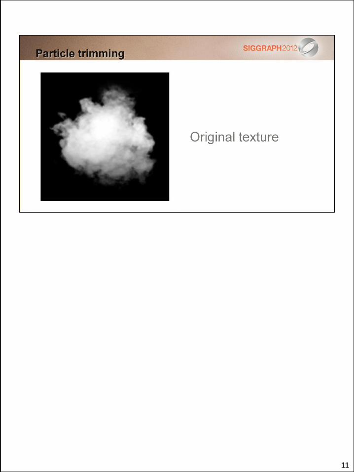
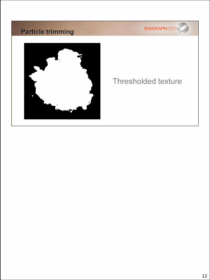
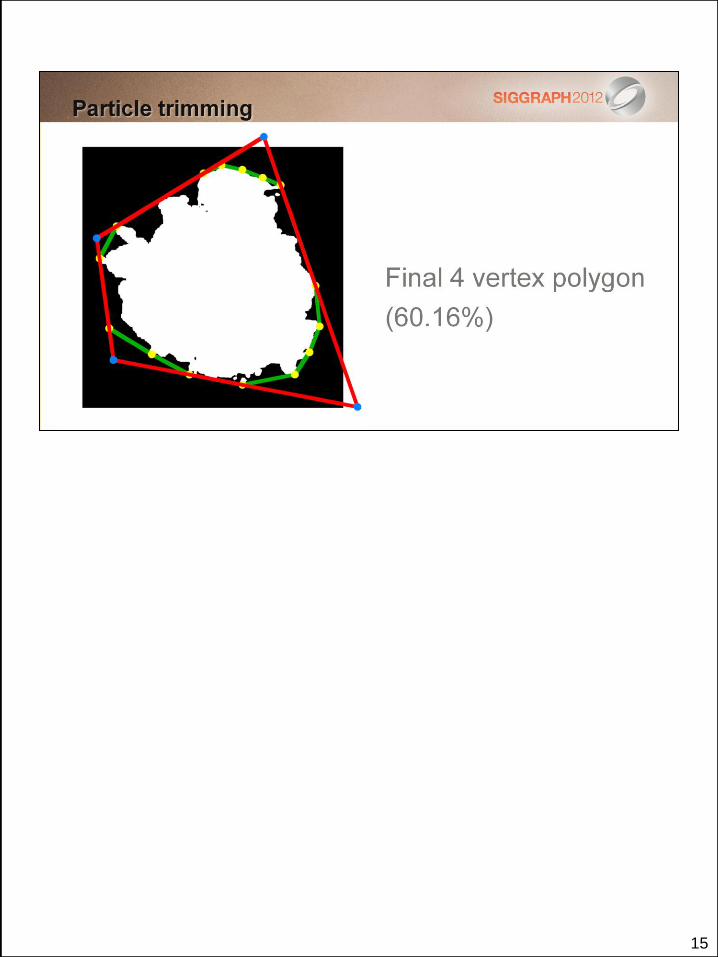
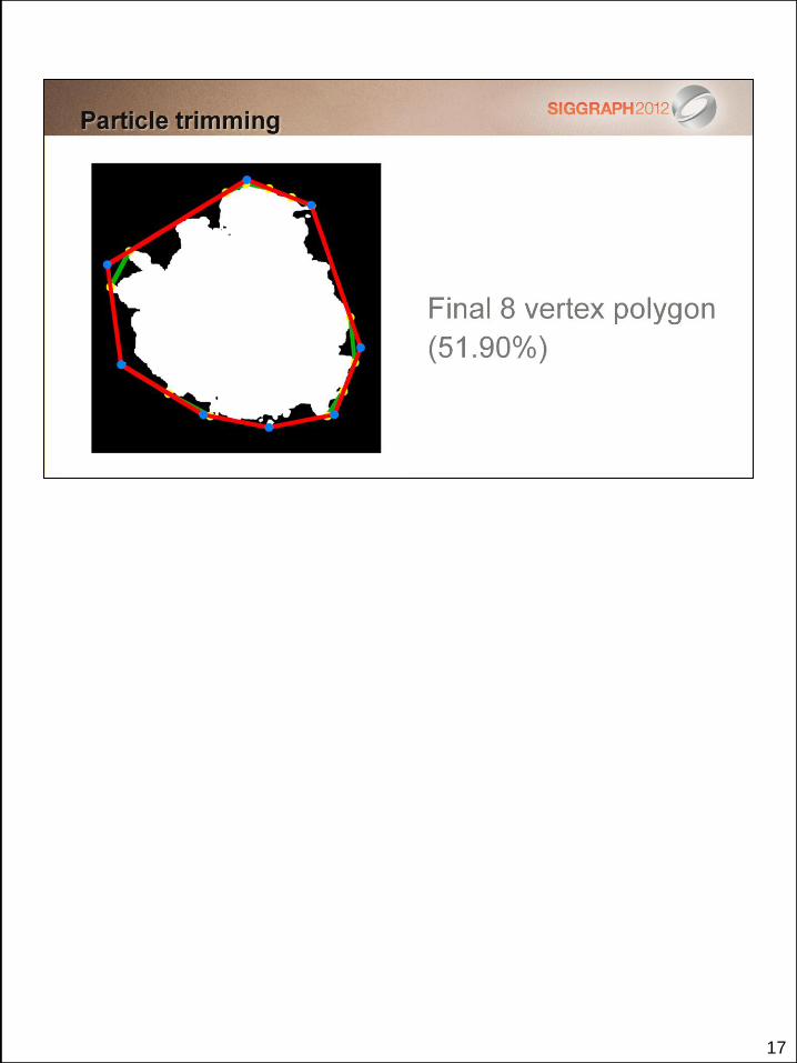
A typical particle texture has plenty of area where alpha is zero. Rendering those pixels will be

a waste of fillrate as it contributes nothing to the final frame.

Instead of simply drawing a plain quad, a better approach is to use irregular polygons that

tightly encloses the ”meat” of the particle. We made a tool that automatically finds an optimal

enclosing polygon for a given texture.

8

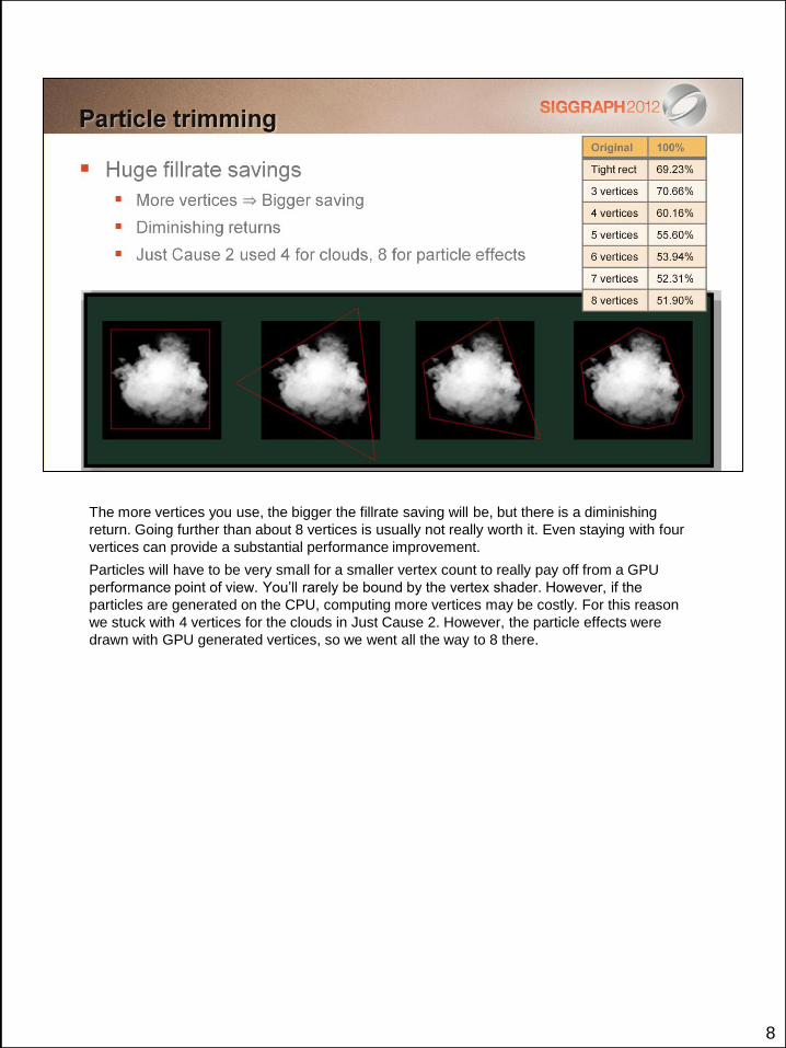
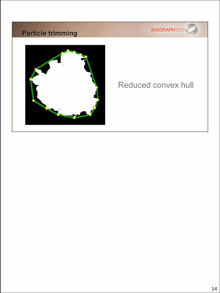
The more vertices you use, the bigger the fillrate saving will be, but there is a diminishing

return. Going further than about 8 vertices is usually not really worth it. Even staying with four

vertices can provide a substantial performance improvement.

Particles will have to be very small for a smaller vertex count to really pay off from a GPU

performance point of view. You’ll rarely be bound by the vertex shader. However, if the

particles are generated on the CPU, computing more vertices may be costly. For this reason

we stuck with 4 vertices for the clouds in Just Cause 2. However, the particle effects were

drawn with GPU generated vertices, so we went all the way to 8 there.

9

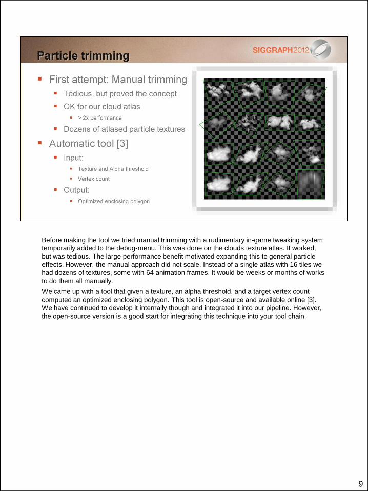
Before making the tool we tried manual trimming with a rudimentary in-game tweaking system

temporarily added to the debug-menu. This was done on the clouds texture atlas. It worked,

but was tedious. The large performance benefit motivated expanding this to general particle

effects. However, the manual approach did not scale. Instead of a single atlas with 16 tiles we

had dozens of textures, some with 64 animation frames. It would be weeks or months of works

to do them all manually.

We came up with a tool that given a texture, an alpha threshold, and a target vertex count

computed an optimized enclosing polygon. This tool is open-source and available online [3].

We have continued to develop it internally though and integrated it into our pipeline. However,

the open-source version is a good start for integrating this technique into your tool chain.

10

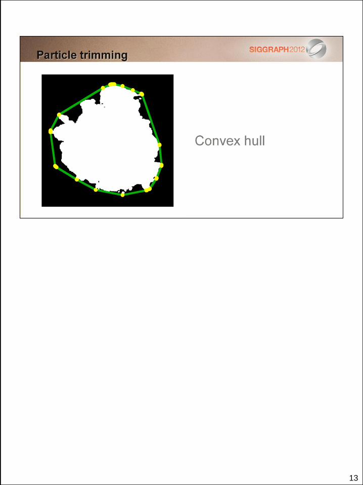
Adding pixels to the convex hull can be quite slow if we are adding every solid pixel. So

whenever a pixel is deemed to not be a potential corner pixel, e.g. it is surrounded by other

solid pixel and thus completely within solid space, then we simply skip it. This made the

construction of the convex hull substantially faster.

The convex hull is typically a fair bit larger than the target vertex count, anything from a few

dozen up to hundreds of vertices. To find the most optimal polygon we loop through all

permutation of edges in the hull and select the one that results in the smallest area. This is a

brute-force approach, so it is important to reduce the search space prior to this selection

phase. So we remove vertices from the convex hull, one-by-one, by finding the edge that

grows the convex hull the least when removed.

11

12

13

14

15

16

17

18

The optimized polygons can sometimes include long sharp wedges that extend outside of the

original quad. For a regular texture this is fine, just use CLAMP mode. For texture atlases this

could mean that part of the ”meat” from another particle gets included, which produces ugly

artifacts. This is generally only a problem in practice for small vertex counts, like 3-5 vertices.

In Just Cause 2 we used 8 vertices, so this was not a problem. For the clouds texture that used

4 vertices this was avoided manually as part of the tweaking, which occasionally led to

somewhat larger polygons than otherwise necessary. Post-JC2 we have added a proper

solution that simply rejects solutions where the resulting polygon would intersect the convex

hull of another atlas tile. This typically allows a fair amount of cutting into neighboring quads,

but never into the actual particle.

19

20

When reducing the number of draw calls there are two standard approaches. Multiple

instances of a single mesh is typically done with regular instancing. If there are multiple

meshes, but a single instance of each, they can be merged into a single vertex and index

buffer and drawn with a single draw call. However, sometimes you want to draw multiple

meshes, with multiple instances of each, and each with their own transforms or other instance

data. With instancing this results in multiple draw calls. With the standard merging approach

you need to duplicate the vertex data.

We came up with an approach that combine the benefits of merging and instancing such that

you can draw it all with a single draw call without duplicating vertex data. Thus, for the lack of a

better name, it can be referred to as Merge-Instancing.

21

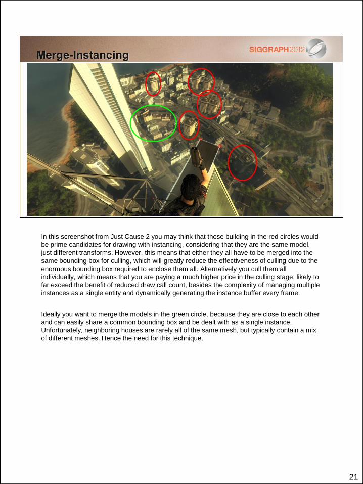
In this screenshot from Just Cause 2 you may think that those building in the red circles would

be prime candidates for drawing with instancing, considering that they are the same model,

just different transforms. However, this means that either they all have to be merged into the

same bounding box for culling, which will greatly reduce the effectiveness of culling due to the

enormous bounding box required to enclose them all. Alternatively you cull them all

individually, which means that you are paying a much higher price in the culling stage, likely to

far exceed the benefit of reduced draw call count, besides the complexity of managing multiple

instances as a single entity and dynamically generating the instance buffer every frame.

Ideally you want to merge the models in the green circle, because they are close to each other

and can easily share a common bounding box and be dealt with as a single instance.

Unfortunately, neighboring houses are rarely all of the same mesh, but typically contain a mix

of different meshes. Hence the need for this technique.

22

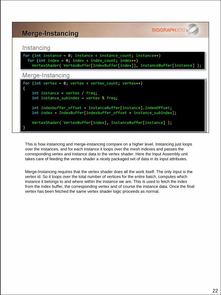
This is how instancing and merge-instancing compare on a higher level. Instancing just loops

over the instances, and for each instance it loops over the mesh indexes and passes the

corresponding vertex and instance data to the vertex shader. Here the Input Assembly unit

takes care of feeding the vertex shader a nicely packaged set of data in its input attributes.

Merge-Instancing requires that the vertex shader does all the work itself. The only input is the

vertex id. So it loops over the total number of vertices for the entire batch, computes which

instance it belongs to and where within the instance we are. This is used to fetch the index

from the index buffer, the corresponding vertex and of course the instance data. Once the final

vertex has been fetched the same vertex shader logic proceeds as normal.

23

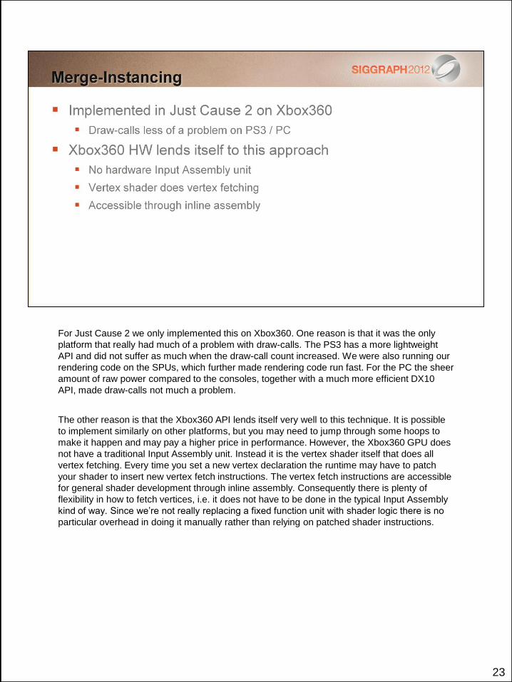
For Just Cause 2 we only implemented this on Xbox360. One reason is that it was the only

platform that really had much of a problem with draw-calls. The PS3 has a more lightweight

API and did not suffer as much when the draw-call count increased. We were also running our

rendering code on the SPUs, which further made rendering code run fast. For the PC the sheer

amount of raw power compared to the consoles, together with a much more efficient DX10

API, made draw-calls not much a problem.

The other reason is that the Xbox360 API lends itself very well to this technique. It is possible

to implement similarly on other platforms, but you may need to jump through some hoops to

make it happen and may pay a higher price in performance. However, the Xbox360 GPU does

not have a traditional Input Assembly unit. Instead it is the vertex shader itself that does all

vertex fetching. Every time you set a new vertex declaration the runtime may have to patch

your shader to insert new vertex fetch instructions. The vertex fetch instructions are accessible

for general shader development through inline assembly. Consequently there is plenty of

flexibility in how to fetch vertices, i.e. it does not have to be done in the typical Input Assembly

kind of way. Since we’re not really replacing a fixed function unit with shader logic there is no

particular overhead in doing it manually rather than relying on patched shader instructions.

24

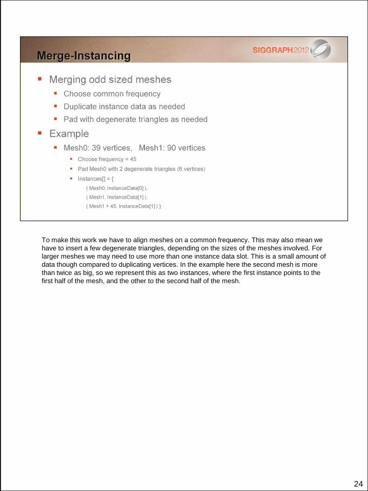
To make this work we have to align meshes on a common frequency. This may also mean we

have to insert a few degenerate triangles, depending on the sizes of the meshes involved. For

larger meshes we may need to use more than one instance data slot. This is a small amount of

data though compared to duplicating vertices. In the example here the second mesh is more

than twice as big, so we represent this as two instances, where the first instance points to the

first half of the mesh, and the other to the second half of the mesh.

25

26

At one point aliasing was sort of a solved problem, first through mipmapping for the shading

and later through MSAA for geometric edges. However, aliasing in games is on the rise again.

As shaders get more advanced mipmapping alone does not fully solve the shader aliasing

problem. More complex lighting introduces aliasing where the mipmapped textures alone

exhibit none. In particular the specular component tends to cause lots of aliasing. This field is

poorly researched and only quite few approaches exist to properly deal with the problem. The

most notable work here is LEAN mapping. On the geometry side we are getting increasingly

denser geometry, and as geometry gets down to the sub-pixel level, MSAA is not always

sufficient.

27

This technique takes a stab at solving the thin geometry case, at least for a subset of common

content in games exhibiting an aliasing problem, in particular phone-wires.

28

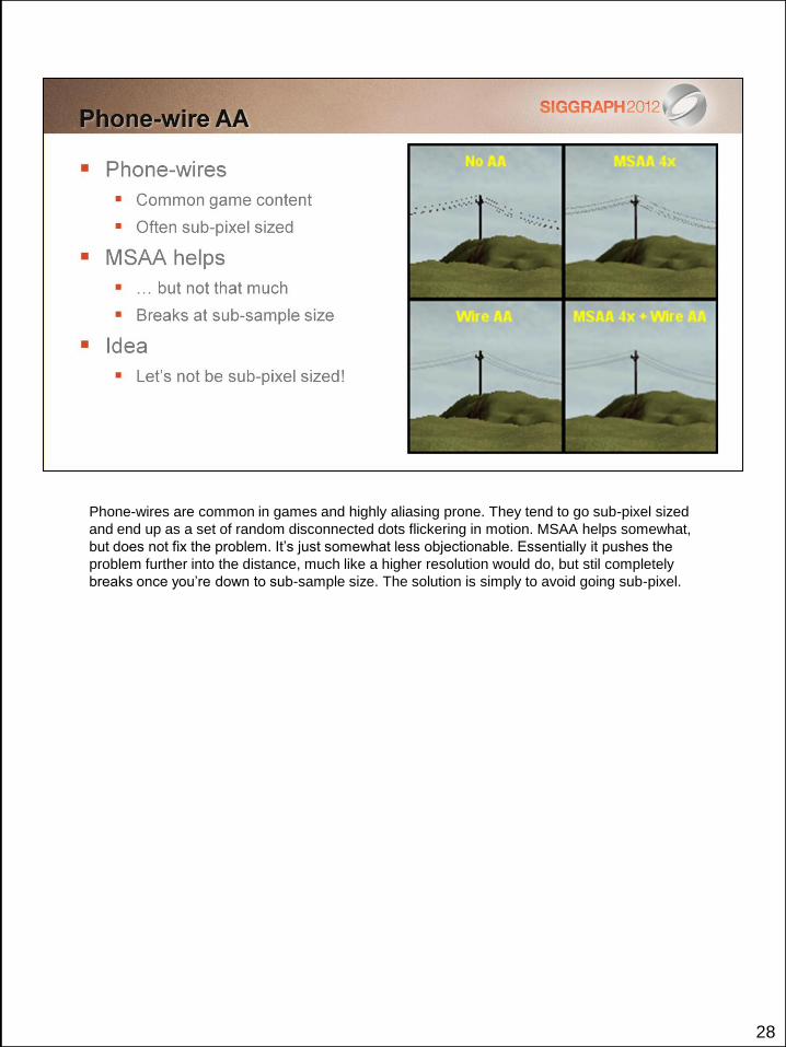
Phone-wires are common in games and highly aliasing prone. They tend to go sub-pixel sized

and end up as a set of random disconnected dots flickering in motion. MSAA helps somewhat,

but does not fix the problem. It’s just somewhat less objectionable. Essentially it pushes the

problem further into the distance, much like a higher resolution would do, but stil completely

breaks once you’re down to sub-sample size. The solution is simply to avoid going sub-pixel.

29

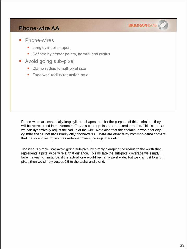
Phone-wires are essentially long cylinder shapes, and for the purpose of this technique they

will be represented in the vertex buffer as a center point, a normal and a radius. This is so that

we can dynamically adjust the radius of the wire. Note also that this technique works for any

cylinder shape, not necessarily only phone-wires. There are other fairly common game content

that it also applies to, such as antenna towers, railings, bars etc.

The idea is simple. We avoid going sub-pixel by simply clamping the radius to the width that

represents a pixel wide wire at that distance. To simulate the sub-pixel coverage we simply

fade it away, for instance, if the actual wire would be half a pixel wide, but we clamp it to a full

pixel, then we simply output 0.5 to the alpha and blend.

30

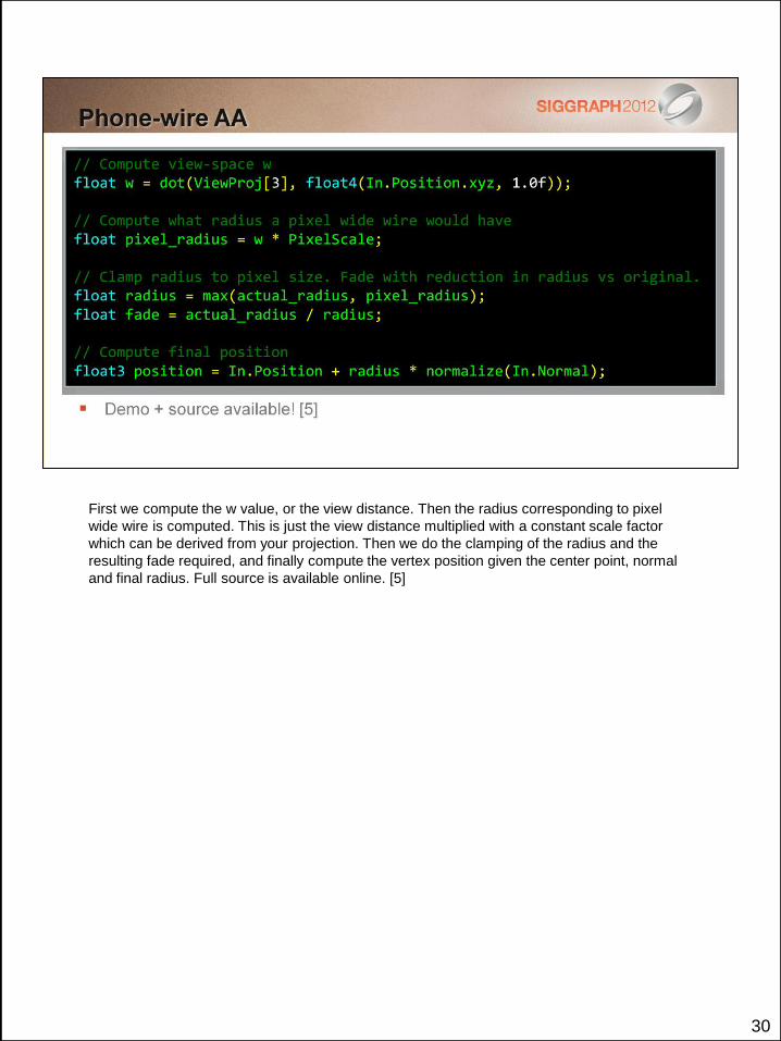
First we compute the w value, or the view distance. Then the radius corresponding to pixel

wide wire is computed. This is just the view distance multiplied with a constant scale factor

which can be derived from your projection. Then we do the clamping of the radius and the

resulting fade required, and finally compute the vertex position given the center point, normal

and final radius. Full source is available online. [5]

31

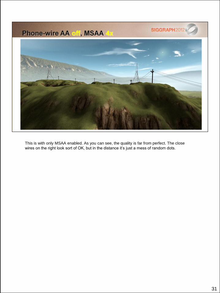
This is with only MSAA enabled. As you can see, the quality is far from perfect. The close

wires on the right look sort of OK, but in the distance it’s just a mess of random dots.

32

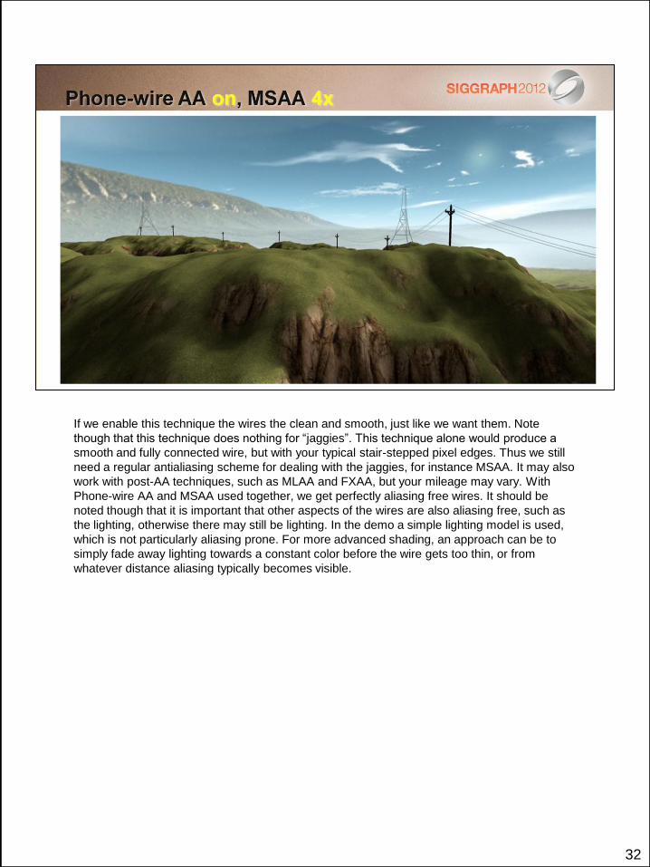
If we enable this technique the wires the clean and smooth, just like we want them. Note

though that this technique does nothing for “jaggies”. This technique alone would produce a

smooth and fully connected wire, but with your typical stair-stepped pixel edges. Thus we still

need a regular antialiasing scheme for dealing with the jaggies, for instance MSAA. It may also

work with post-AA techniques, such as MLAA and FXAA, but your mileage may vary. With

Phone-wire AA and MSAA used together, we get perfectly aliasing free wires. It should be

noted though that it is important that other aspects of the wires are also aliasing free, such as

the lighting, otherwise there may still be lighting. In the demo a simple lighting model is used,

which is not particularly aliasing prone. For more advanced shading, an approach can be to

simply fade away lighting towards a constant color before the wire gets too thin, or from

whatever distance aliasing typically becomes visible.

33

34

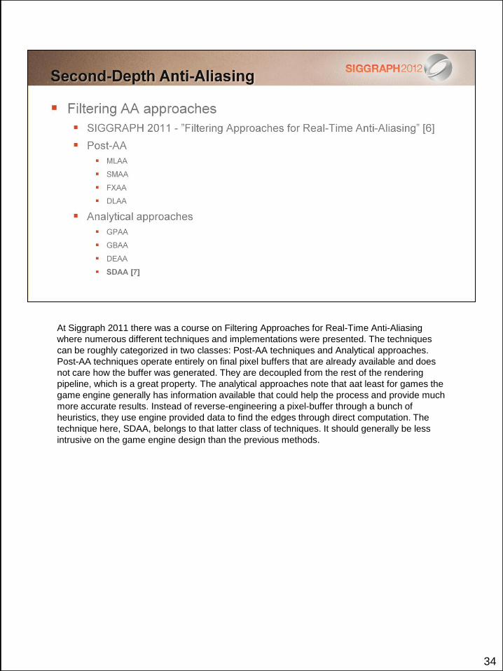
At Siggraph 2011 there was a course on Filtering Approaches for Real-Time Anti-Aliasing

where numerous different techniques and implementations were presented. The techniques

can be roughly categorized in two classes: Post-AA techniques and Analytical approaches.

Post-AA techniques operate entirely on final pixel buffers that are already available and does

not care how the buffer was generated. They are decoupled from the rest of the rendering

pipeline, which is a great property. The analytical approaches note that aat least for games the

game engine generally has information available that could help the process and provide much

more accurate results. Instead of reverse-engineering a pixel-buffer through a bunch of

heuristics, they use engine provided data to find the edges through direct computation. The

technique here, SDAA, belongs to that latter class of techniques. It should generally be less

intrusive on the game engine design than the previous methods.

35

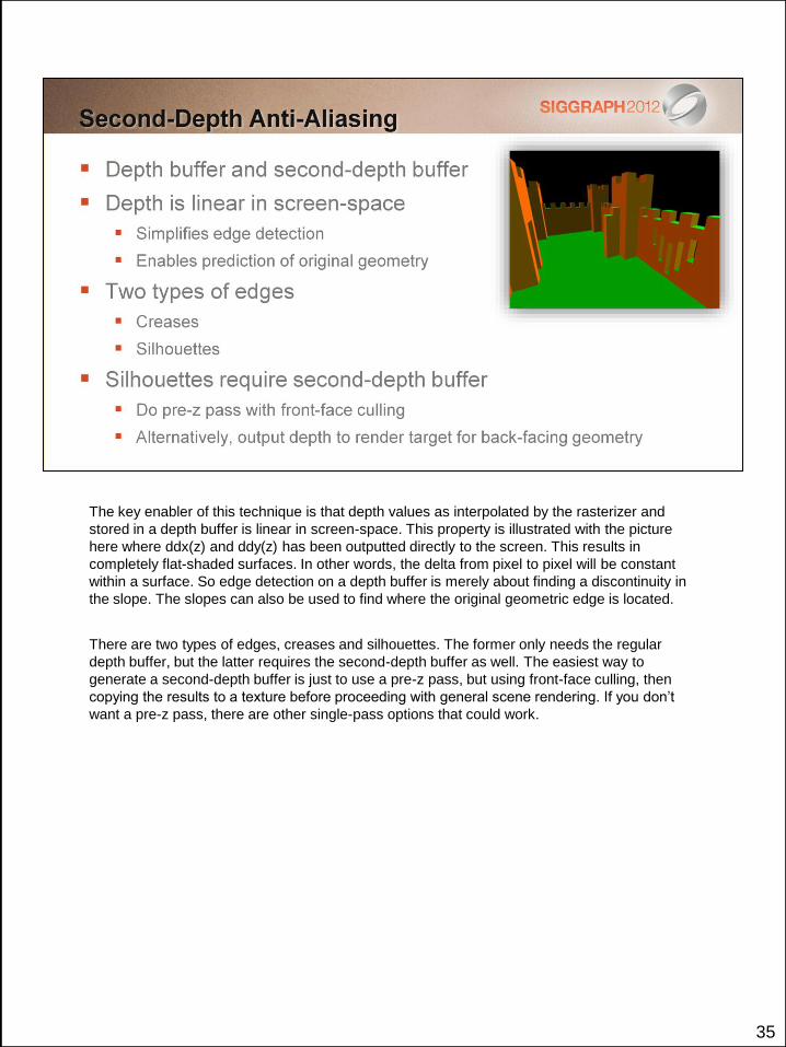
The key enabler of this technique is that depth values as interpolated by the rasterizer and

stored in a depth buffer is linear in screen-space. This property is illustrated with the picture

here where ddx(z) and ddy(z) has been outputted directly to the screen. This results in

completely flat-shaded surfaces. In other words, the delta from pixel to pixel will be constant

within a surface. So edge detection on a depth buffer is merely about finding a discontinuity in

the slope. The slopes can also be used to find where the original geometric edge is located.

There are two types of edges, creases and silhouettes. The former only needs the regular

depth buffer, but the latter requires the second-depth buffer as well. The easiest way to

generate a second-depth buffer is just to use a pre-z pass, but using front-face culling, then

copying the results to a texture before proceeding with general scene rendering. If you don’t

want a pre-z pass, there are other single-pass options that could work.

36

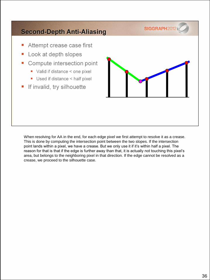
When resolving for AA in the end, for each edge pixel we first attempt to resolve it as a crease.

This is done by computing the intersection point between the two slopes. If the intersection

point lands within a pixel, we have a crease. But we only use it if it’s within half a pixel. The

reason for that is that if the edge is further away than that, it is actually not touching this pixel’s

area, but belongs to the neighboring pixel in that direction. If the edge cannot be resolved as a

crease, we proceed to the silhouette case.

37

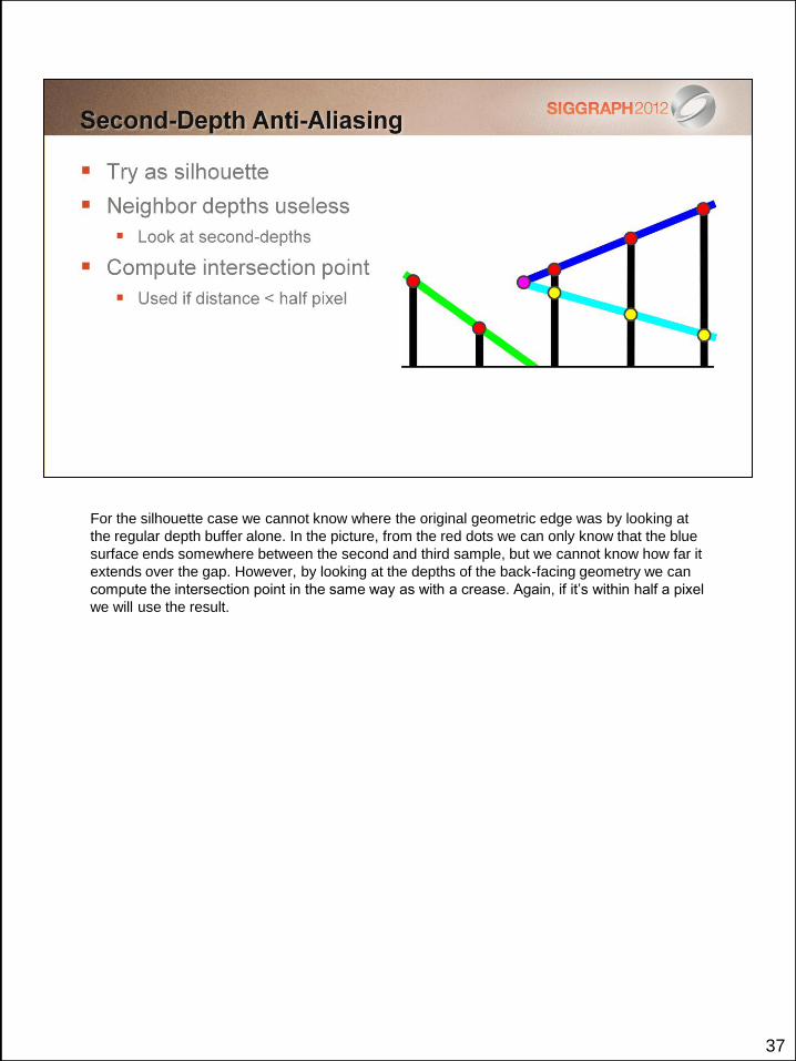
For the silhouette case we cannot know where the original geometric edge was by looking at

the regular depth buffer alone. In the picture, from the red dots we can only know that the blue

surface ends somewhere between the second and third sample, but we cannot know how far it

extends over the gap. However, by looking at the depths of the back-facing geometry we can

compute the intersection point in the same way as with a crease. Again, if it’s within half a pixel

we will use the result.

38

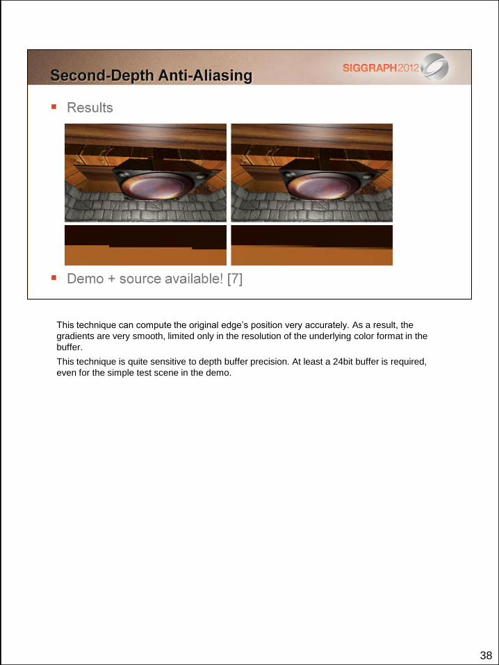
This technique can compute the original edge’s position very accurately. As a result, the

gradients are very smooth, limited only in the resolution of the underlying color format in the

buffer.

This technique is quite sensitive to depth buffer precision. At least a 24bit buffer is required,

even for the simple test scene in the demo.

39

40