Graphical Modelsand

Conditional Random Fields

Presenter: Shih-Hsiang Lin

Bishop, C. M., “Pattern Recognition and Machine Learning,” Springer, 2006Sutton, C., McCallum, A., “An Introduction to Conditional Random Fields for Relational Learning,” Introduction to Statistical Relational Learning, MIT Press. 2007Rahul Gupta, “Conditional Random Fields,” Dept. of Computer Science and Engg., IIT Bombay, India.

2

Overview

• Introduction to graphical models• Applications of graphical models• More detail on conditional random fields• Conclusions

Introduction to Graphical Models

4

Power of Probabilistic Graphical Models

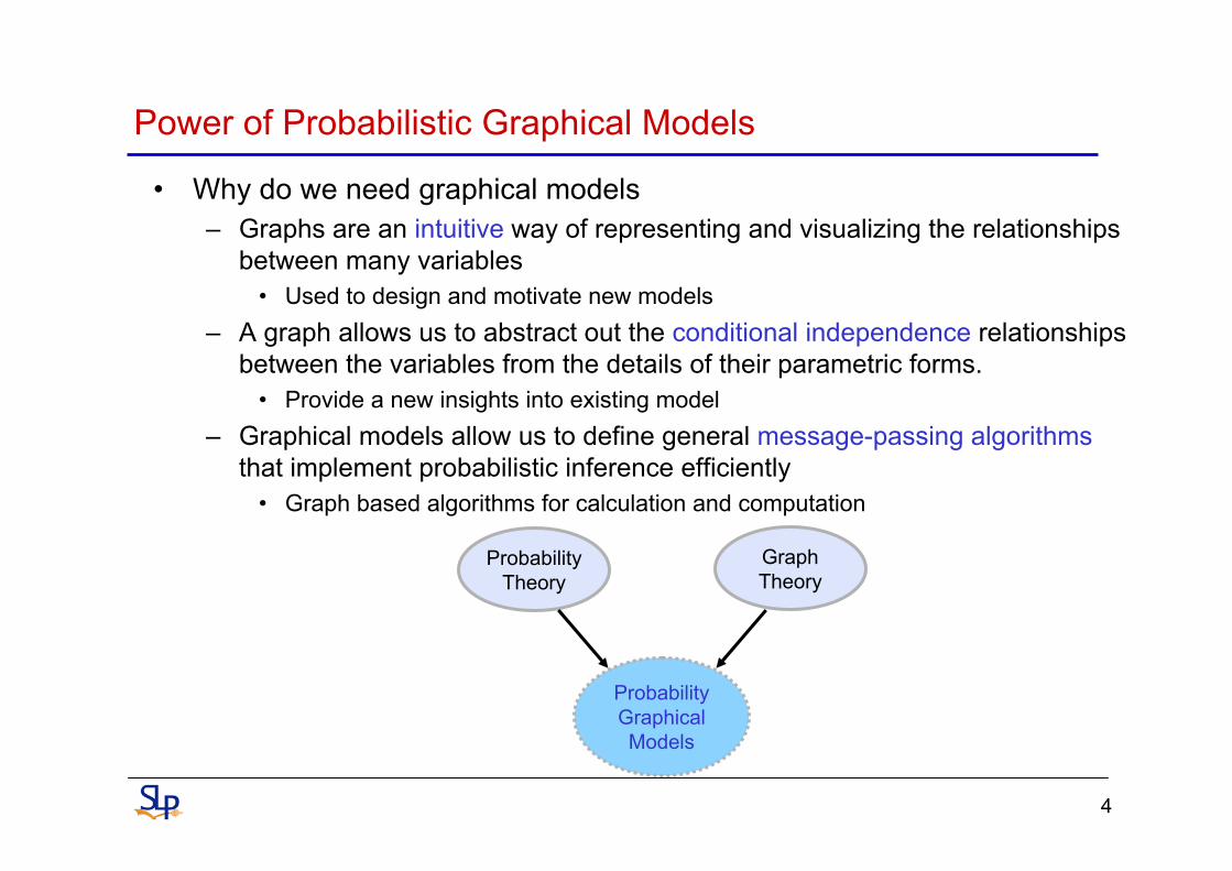
• Why do we need graphical models– Graphs are an intuitive way of representing and visualizing the relationships

between many variables• Used to design and motivate new models

– A graph allows us to abstract out the conditional independence relationships between the variables from the details of their parametric forms.

• Provide a new insights into existing model– Graphical models allow us to define general message-passing algorithms

that implement probabilistic inference efficiently• Graph based algorithms for calculation and computation

ProbabilityTheory

GraphTheory

ProbabilityGraphicalModels

5

Probability Theory

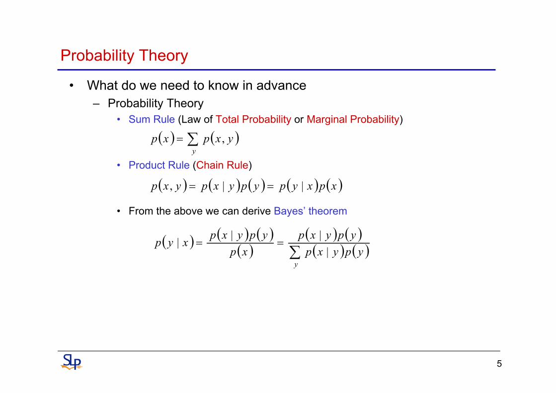
• What do we need to know in advance– Probability Theory

• Sum Rule (Law of Total Probability or Marginal Probability)

• Product Rule (Chain Rule)

• From the above we can derive Bayes’ theorem

( ) ( )∑=y

yxpxp ,

( ) ( ) ( ) ( ) ( )xpxypypyxpyxp ||, ==

( ) ( ) ( )( )

( ) ( )( ) ( )∑

==

yypyxpypyxp

xpypyxpxyp

||||

6

Conditional Independence and Marginal Independence

• Conditional Independence

which is equivalent to saying

– Conditional independence crucial in practical applications since we can rarely work with a general joint distribution

• Marginal Independence

• Example– Amount of Speeding Fine Type of Car | Speed– Lung Cancer Yellow Teeth | Smoking– Child’s Genes Grandparents’ Genes | Parents’ Genes– Ability of Team A Ability of Team B

( ) ( ) ( ) ( ) ( )zypzxpzypzyxpzyxp |||,||, ==

( ) ( )zxpzyxp |,| =z|y x ⇔

( ) ( ) ( )ypxpyxp =,y x ⇔ 0|b aempty set

⇔

7

Graphical models

• A graphical model comprises nodes connected by links– Nodes (vertices) correspond to random variables– Links (edges or arcs) represents the relationships between the variables

• Directed graphs are useful for expressing casual relationshipsbetween random variables

• Undirected graphs are better suited to expressing soft constraintsbetween random variables

a

c

b

Undirected Graph

a

c

b

Directed Graph

8

Directed Graphs

• Consider an arbitrary distribution , we can write the joint distribution in the form– By successive application of the product rule

• We then can represent the above equation in terms of a simple graphical models– First, we introduce a node for each of the random variables– Second, for each conditional distribution we add directed links to the

graph

( )cbap ,,

( ) ( ) ( )bapbacpcbap ,,|,, =

( ) ( ) ( ) ( )apabpbacpcbap |,|,, =

* Note that this decomposition holds for any choice of joint distributionor

a

cb

A fully connected graph

9

Directed Graphs (cont.)

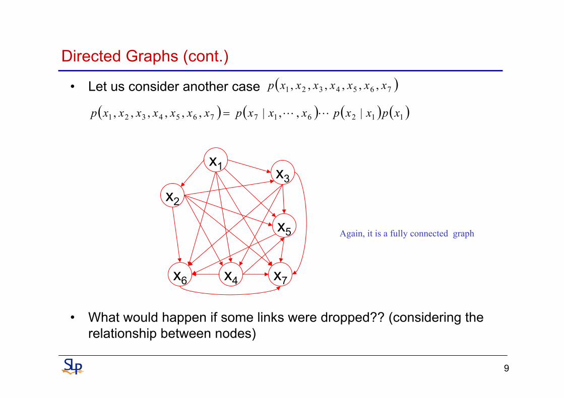
• Let us consider another case

• What would happen if some links were dropped?? (considering the relationship between nodes)

( )7654321 ,,,,,, xxxxxxxp

( ) ( ) ( ) ( )1126177654321 |,,|,,,,,, xpxxpxxxpxxxxxxxp LL=

x1

x7

x2

x3

x4

x5

x6

Again, it is a fully connected graph

10

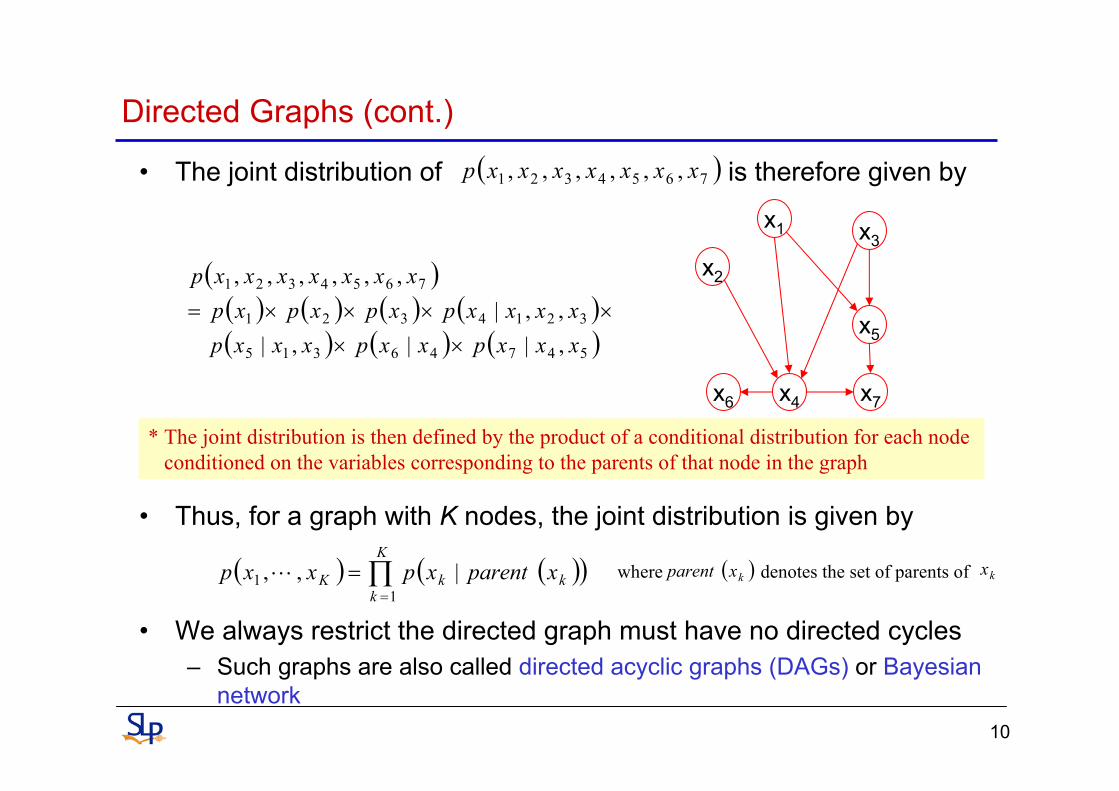
• The joint distribution of is therefore given by

• Thus, for a graph with K nodes, the joint distribution is given by

• We always restrict the directed graph must have no directed cycles– Such graphs are also called directed acyclic graphs (DAGs) or Bayesian

network

where denotes the set of parents of

Directed Graphs (cont.)

x1

x7

x2

x3

x4

x5

x6

( )7654321 ,,,,,, xxxxxxxp

( )( ) ( ) ( ) ( )( ) ( ) ( )54746315

3214321

7654321

,||,| ,,|

,,,,,,

xxxpxxpxxxpxxxxpxpxpxp

xxxxxxxp

××××××=

* The joint distribution is then defined by the product of a conditional distribution for each node conditioned on the variables corresponding to the parents of that node in the graph

( ) ( )( )∏=

=K

kkkK xparentxpxxp

11 |,,L ( )kxparent kx

11

Directed Graph: Conditional Independence

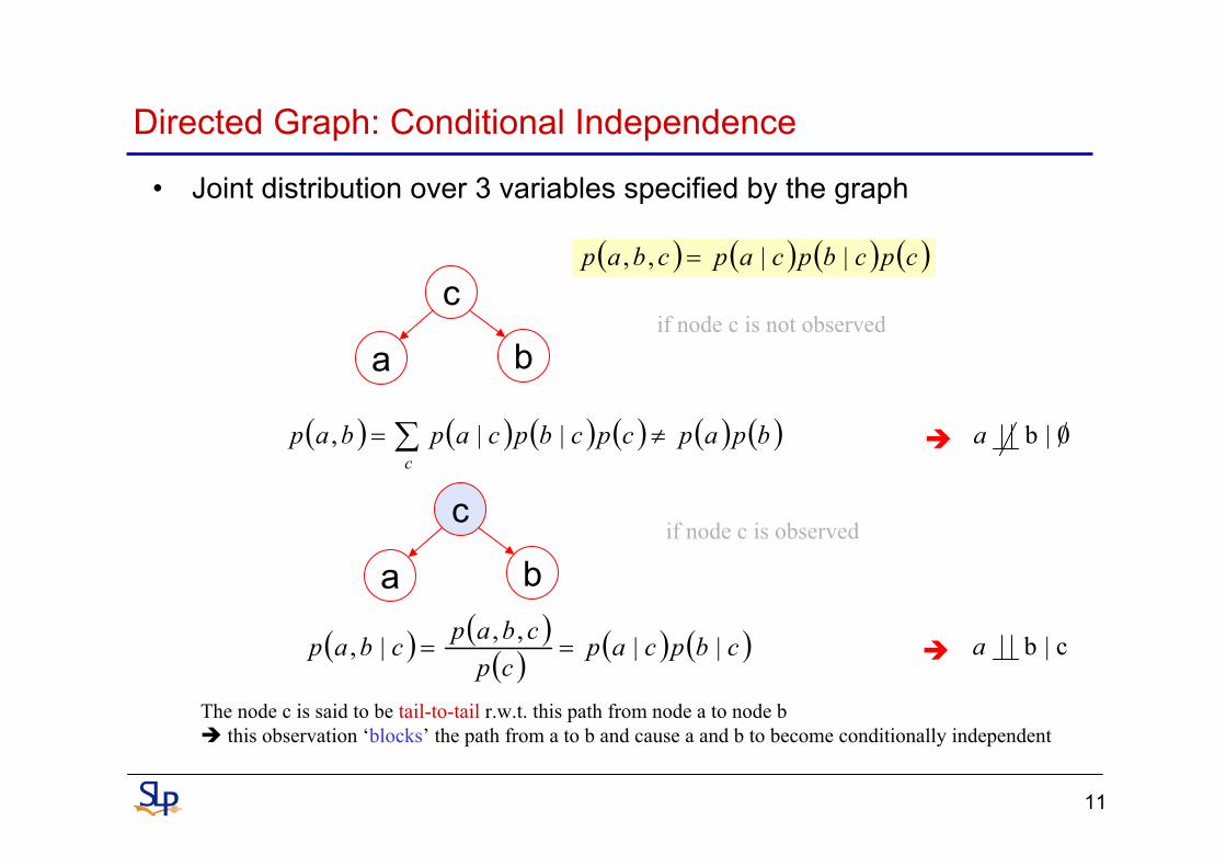
• Joint distribution over 3 variables specified by the graph

a

c

bif node c is observed

( ) ( )( ) ( ) ( )cbpcapcpcbapcbap ||,,|, == c|b a

a

c

bif node c is not observed

( ) ( ) ( ) ( ) ( ) ( )bpapcpcbpcapbapc

≠= ∑ ||, 0|b a

The node c is said to be tail-to-tail r.w.t. this path from node a to node bthis observation ‘blocks’ the path from a to b and cause a and b to become conditionally independent

( ) ( ) ( ) ( )cpcbpcapcbap ||,, =

12

Directed Graph: Conditional Independence (cont.)

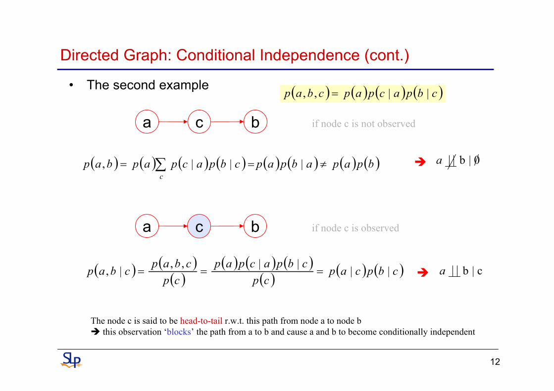
• The second example

a c b

( ) ( )( )

( ) ( ) ( )( ) ( ) ( )cbpcapcp

cbpacpapcpcbapcbap ||||,,|, ===

if node c is observed

c|b a

a c b if node c is not observed

( ) ( ) ( ) ( ) ( ) ( ) ( ) ( )bpapabpapcbpacpapbapc

≠== ∑ |||, 0|b a

The node c is said to be head-to-tail r.w.t. this path from node a to node bthis observation ‘blocks’ the path from a to b and cause a and b to become conditionally independent

( ) ( ) ( ) ( )cbpacpapcbap ||,, =

13

Directed Graph: Conditional Independence (cont.)

• The third example

a

c

bif node c is not observed

( ) ( ) ( ) ( ) ( ) ( ) ( )bpapbacpbpapcbapbapcc

=== ∑∑ ,|,,,

( ) ( ) ( ) ( )bacpbpapcbap ,|,, =

0|b a

a

c

bif node c is observed

( ) ( )( )

( ) ( ) ( )( ) ( ) ( )cbpcapcp

bacpbpapcpcbapcbap ||,|,,|, ≠== c|b a

The node c is said to be head-to-head r.w.t. this path from node a to node bthe conditioned node c ‘unblocks’ the path and renders a and b dependent

14

D-separation

• if C d-separated A from B– We need to consider all possible paths from any node in A to any node in B– Any such path is said to be blocked if it includes a node such that either

(a) the arrows on the path meet either head-to-tail or tail-to-tail at the node, and the node is in the set C

(b) the arrows meet head-to-tail at the node, and neither the node, nor any of its descendants, is in the set C

– If all paths are blocked, then A is said to be d-separated from B by C

C|B A

a

e

f

b

c

a

e

f

b

cc|b a f|b a

15

Markov Blankets

• Markov blankets (or Markov boundary) of a node x is the minimal set of nodes that isolates nodes A from the rest of the graph– Every set of nodes in the network is conditionally independent of A when

conditioned on the Markov blanket of the node A

– MB(A)= {parents(A) and children(A) and parents-of-children(A)}( )( ) ( )( )AMBApBAMBAp || =∩

AA

16

Examples of Directed Graphs

• Hidden Markov models• Kalman filters• Factor analysis• Probabilistic principal component analysis• Independent component analysis• Mixtures of Gaussians• Transformed component analysis• Probabilistic expert systems• Sigmoid belief networks• Hierarchical mixtures of experts• etc,…

17

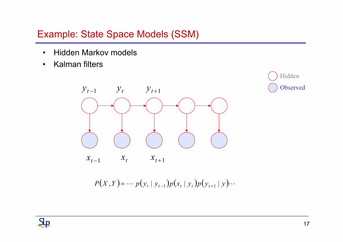
Example: State Space Models (SSM)

• Hidden Markov models• Kalman filters

tx 1+tx1−tx

ty 1+ty1−tyHidden

Observed

( ) ( ) ( ) ( )LL yypyxpyypYXP ttttt |||, 11 +−=

18

Example: Factorial SSM

• Multiple hidden sequences

Hidden

Observed

19

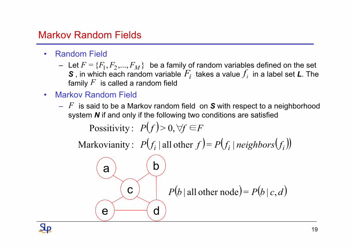
Markov Random Fields

• Random Field– Let be a family of random variables defined on the set S , in which each random variable takes a value in a label set L. The family is called a random field

• Markov Random Field– is said to be a Markov random field on S with respect to a neighborhood

system N if and only if the following two conditions are satisfied

},...,,{= 21 MFFFFiF if

F

F

( ) FffP ∈∀,0> :yPossitivit( ) ( )( )iii fneighborsfPffP |=other all| :tyMarkoviani

a

d

b

c

e

( ) ( )dcbPbP ,|=nodeother all|

20

Undirected Graphs

• An undirected graphical model can also called Markov random fields, or also known as a Markov networks– It has a set of nodes each of which corresponds to a variable of group of

variables, as well as a set of links each of which connects a pair of nodes• In an undirected graphical models, the joint distribution is product of

non-negative functions over the cliques of the graph

( ) ( )∏=C

CC xZxp ψ1 where are the clique potential, and is a

normalization constant (sometimes called the partition function)( )CC xψ Z

a

d

b

c

e

( ) ( ) ( ) ( )edcdcbcaZ

xp CBA ,,,,,1 ψψψ=

A B

C

21

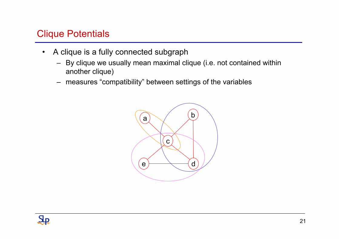
Clique Potentials

• A clique is a fully connected subgraph– By clique we usually mean maximal clique (i.e. not contained within

another clique)– measures “compatibility” between settings of the variables

a

d

b

c

e

22

Undirected Graphs: Conditional Independence

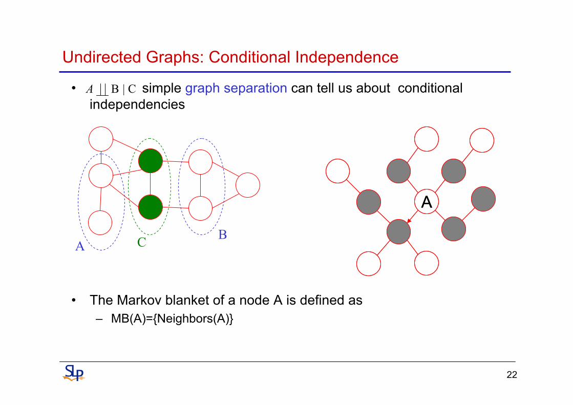
• simple graph separation can tell us about conditional independencies

• The Markov blanket of a node A is defined as– MB(A)={Neighbors(A)}

C|B A

A C B

AA

23

Examples of Undirected Graphs

• Markov Random Fields• Condition Random Fields• Maximum Entropy Markov Models• Maximum Entropy• Boltzmann Machines• etc,…

24

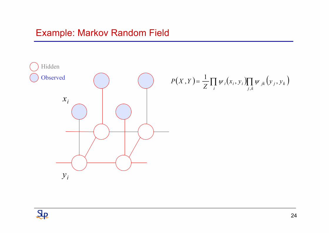
Example: Markov Random Field

ix

iy

( ) ( ) ( )∏∏=kj

kjjki

iii yyyxZ

YXP,

,,1, ψψ

Hidden

Observed

25

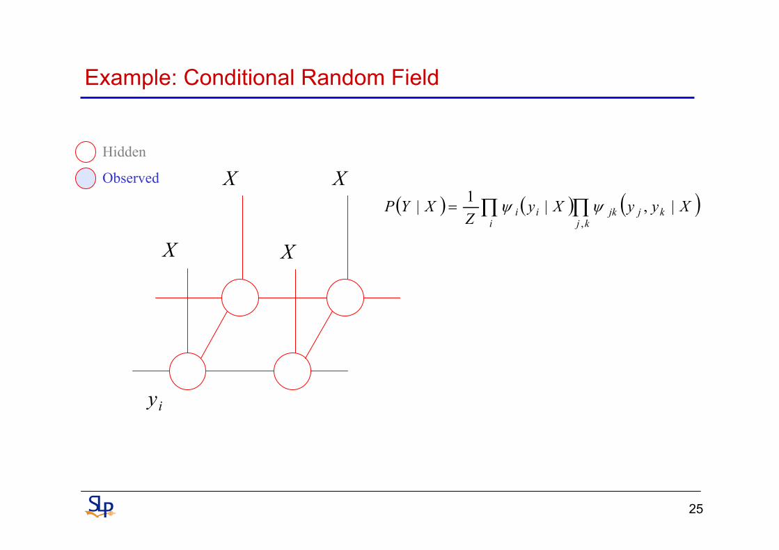
Example: Conditional Random Field

X

iy

( ) ( ) ( )∏∏=kj

kjjki

ii XyyXyZ

XYP,

|,|1| ψψ

X X

X

Hidden

Observed

26

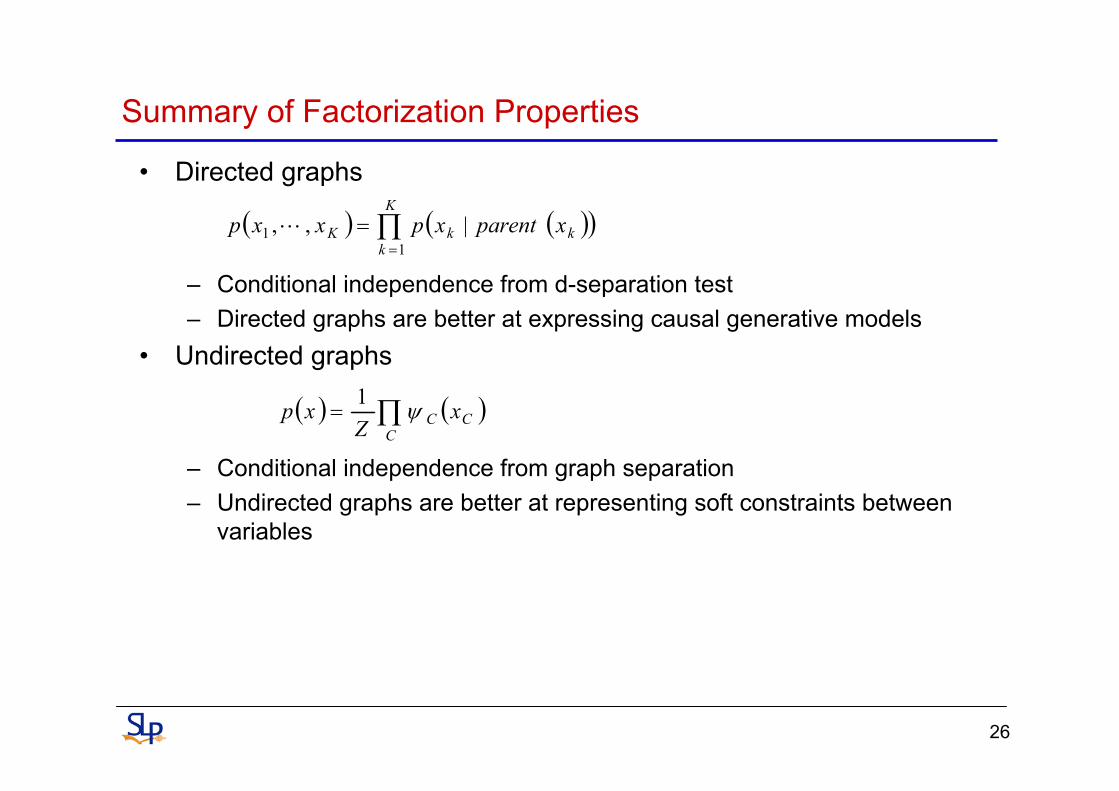
Summary of Factorization Properties

• Directed graphs

– Conditional independence from d-separation test– Directed graphs are better at expressing causal generative models

• Undirected graphs

– Conditional independence from graph separation– Undirected graphs are better at representing soft constraints between

variables

( ) ( )( )∏=

=K

kkkK xparentxpxxp

11 |,,L

( ) ( )∏=C

CC xZxp ψ1

Applications of Graphical Models

28

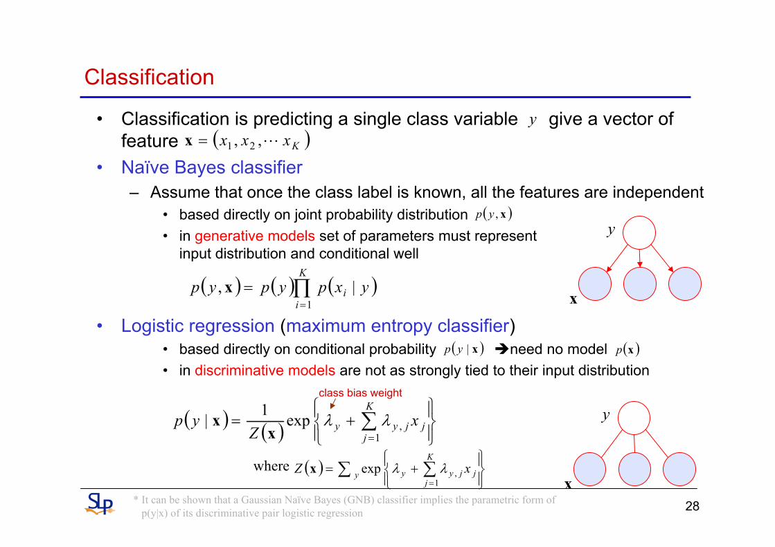
Classification

• Classification is predicting a single class variable give a vector of feature

• Naïve Bayes classifier– Assume that once the class label is known, all the features are independent

• based directly on joint probability distribution • in generative models set of parameters must represent

input distribution and conditional well

• Logistic regression (maximum entropy classifier)• based directly on conditional probability need no model• in discriminative models are not as strongly tied to their input distribution

y( )Kxxx L,, 21=x

( ) ( ) ( )∏=

=K

ii yxpypyp

1|, x

x

y

x

y( ) ( ) ⎪⎭

⎪⎬⎫

⎪⎩

⎪⎨⎧

+= ∑=

K

jjjyy x

Zyp

1,exp1| λλ

xx

( ) ∑ ∑⎪⎭

⎪⎬⎫

⎪⎩

⎪⎨⎧

+==

y

K

jjjyy xZ

1,exp λλxwhere

class bias weight

( )x,yp

( )x|yp ( )xp

* It can be shown that a Gaussian Naïve Bayes (GNB) classifier implies the parametric form ofp(y|x) of its discriminative pair logistic regression

29

Classification (cont.)

• Consider a GNB based on the following modeling assumptions– is a Gaussian distribution of the form– is Boolean, governed by a Bernoulli distribution with parameter

( ) ( ) ( )( ) ( ) ( ) ( )

( ) ( )( ) ( )

( ) ( )( ) ( )

( )( ) ⎟

⎟⎠

⎞⎜⎜⎝

⎛==

+−

+=

⎟⎟⎠

⎞⎜⎜⎝

⎛====

+=

====

+=

==+====

==

∑ ii

i

yxpyxp

ypypypyp

ypypypyp

ypypypypypypyp

1|0|log1logexp1

1

1|10|0logexp1

1

1|10|01

1

0|01|11|1|1

θθ

xx

xx

xxxx

( )ki yyxP =|

( ) ( ) ( )∏=

=K

kk yxpypyp

1|, x

Naïve Bayes

( )iikN σμ .( )1== yPθy

( )( )

( )

( )

( ) ( )

( ) ( )

∑

∑

∑

∑∑

⎟⎟⎠

⎞⎜⎜⎝

⎛ −+

−=

⎟⎟⎠

⎞⎜⎜⎝

⎛ −−−=

⎟⎟⎠

⎞⎜⎜⎝

⎛ −−−=

⎟⎟⎠

⎞⎜⎜⎝

⎛ −−

⎟⎟⎠

⎞⎜⎜⎝

⎛ −−

===

ii

iii

i

ii

ii

iiii

ii

iiii

i

i

ii

i

i

ii

ii

i

i

x

xx

xx

x

x

yxpyxp

2

20

21

210

2

20

21

2

20

21

2

21

2

2

20

2

2

2

2explog

2exp

2

1

2exp

2

1

log1|0|log

πσμμ

σμμ

πσμμ

πσμμ

πσμ

πσ

πσμ

πσ

( )

( )∑

∑

++=

⎟⎟

⎠

⎞

⎜⎜

⎝

⎛⎟⎟⎠

⎞⎜⎜⎝

⎛ −+

−+

−+

==

i ii

ii

iii

i

ii

x

x

yp

λλ

πσμμ

σμμ

θθ

0

2

20

21

210

exp11

21logexp1

1|1 x

30

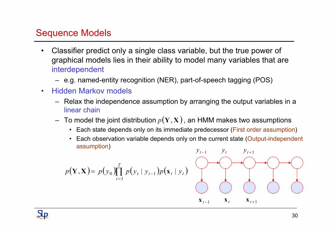
Sequence Models

• Classifier predict only a single class variable, but the true power of graphical models lies in their ability to model many variables that are interdependent– e.g. named-entity recognition (NER), part-of-speech tagging (POS)

• Hidden Markov models– Relax the independence assumption by arranging the output variables in a

linear chain– To model the joint distribution , an HMM makes two assumptions

• Each state depends only on its immediate predecessor (First order assumption)• Each observation variable depends only on the current state (Output-independent

assumption)

( )XY ,p

( ) ( ) ( ) ( )∏=

−=T

ttttt ypyypypp

110 ||, xXY

tx 1+tx1−tx

ty 1+ty1−ty

31

Sequence Models (cont.)

• Maximum Entropy Markov Models (MEMMs)– A conditional model that representing the probability of reaching a state

given an observation and the previous state

– Per-state normalization will cause all the mass that arrives at a state must be distributed among the possible successor states

tx 1+tx1−tx

ty 1+ty1−ty( ) ( ) ( )∏=

−=T

tttt xyypxypp

2111 ,||| XY

( ) ( )⎟⎟⎠

⎞⎜⎜⎝

⎛= ∑ −−

ktttkkttt xyyf

Zxyyp ,,exp1,| 11 λ

( )∑ ∑ ⎟⎟⎠

⎞⎜⎜⎝

⎛= −

'1 ,',exp

y ktttkk xyyfZ λ

* per-state normalization

Label Bias Problem!!!!!Potential victims: Discriminative Models

32

Sequence Models (cont.)

• Label Bias Problem– Consider this MEMM

– P(1 and 2 | ro) = P(2 | 1 and ro)P(1 | ro) = P(2 | 1 and o)P(1 | r)P(1 and 2 | ri) = P(2 | 1 and ri)P(1 | ri) = P(2 | 1 and i)P(1 | r)

– Since P(2 | 1 and x) = 1 for all x, P(1 and 2 | ro) = P(1 and 2 | ri)• In the training data, label 2 is the only label value observed after label 1

Therefore P(2 | 1) = 1, so P(2 | 1 and x) = 1 for all x

– However, we expect P(1 and 2 | ri) to be greater than P(1 and 2 | ro)

33

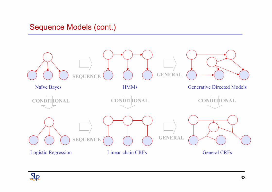
Sequence Models (cont.)

Naïve Bayes

Logistic Regression

Generative Directed Models

Linear-chain CRFs General CRFs

HMMs

CONDITIONAL CONDITIONAL CONDITIONAL

SEQUENCE GENERAL

SEQUENCE GENERAL

34

From HMM to CRFs

• We can rewrite the HMM joint distribution as follows

– Because we do not require the parameter to be log probabilities, we are no longer guaranteed that the distribution sums to 1

• So we explicitly enforce this by using a normalization constant Z

• We can write the above equation more compactly by introducing the concept of feature function

• The last step is to write the conditional distribution

( )xyp ,

( ) ( ) ( ) ( )∏=

−=T

ttttt yxpyypypxyp

110 ||,

HMMs

( ) { } { } { } { }⎟⎟⎠

⎞⎜⎜⎝

⎛+= ∑ ∑ ∑∑ ∑

∈ ∈==

∈== −

t Si Oiyoi

t Sjijyiyij ttttZ

po

oxXY 1111exp1,,

1μλ

( ) ( )⎟⎟⎠

⎞⎜⎜⎝

⎛= ∑

=−

K

ktttkk yyf

Zp

11 ,,exp1, xXY λ

( ) { } { }iyiytttk ttyyf ==− −

=1

11,, 1 x

( ) { } { }oxx ==− = 11,, 1 iytttk tyyf

Feature function for HMMsstate transition

state observation

( )XY |p

( ) ( )( )

( ){ }( ){ }∑ ∑

∑∑ = −

= −==' 1 1

1 1

' ,','exp

,,exp,'

,|y

Kk tttkk

Kk tttkk

yyf

yyfp

ppx

xXY

XYXYY λ

λ

Linear-chain CRFs

More Detail on Conditional Random Fields

36

Conditional Random Fields

• CRFs have all the advantages of MEMMs without label bias problem– MEMM uses per-state exponential model for the conditional probabilities of

next states given the current state– CRF has a single exponential model for the joint probability of the entire

sequence of labels given the observation sequence• Let be a graph such that , so that is indexed

by the vertices of . Then is a conditional random field in case, when conditioned on , the random variables obey the Markovianproperty

( )EVG , ( )VvvY ∈

=Y YG ( )YX ,

X vY

( ) ( )( )vvwv neighborpvwp YXYYXY ,|=≠,,|

1Y 2Y 3Y 4Y 5Y

X( ) ( )4233 ,,|=other all,| YYYpYYp XX

37

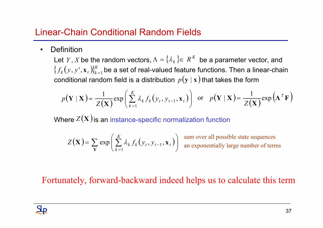
Linear-Chain Conditional Random Fields

• DefinitionLet be the random vectors, be a parameter vector, and

be a set of real-valued feature functions. Then a linear-chainconditional random field is a distribution that takes the form

Where is an instance-specific normalization function

XY ,

( ) ( ) ( )⎟⎟⎠

⎞⎜⎜⎝

⎛= ∑

=−

K

ktttkk yyf

Zp

11 ,,exp1| x

XXY λ

{ } Kk R∈=Λ λ

( ){ }Kktk yyf 1,', =x( )xy |p

( ) ( )∑ ∑ ⎟⎟⎠

⎞⎜⎜⎝

⎛=

=−

YxX

K

ktttkk yyfZ

11 ,,exp λ

( )XZ

( ) ( ) ( )FΛX

XY T

Zp exp1| =or

sum over all possible state sequencesan exponentially large number of terms

Fortunately, forward-backward indeed helps us to calculate this term

38

Forward and Backward Algorithms

• Suppose that we are interested in tagging a sequence only partially, say till the position i– Denote the un-normalized probability of a partial labeling ending at position i

with fixed label y by– Denote the un-normalized probability of a partial segmentation starting at

position i+1 assuming a label y at position i by and can be computed via the following recurrences

– We can now write the marginal and partition function in term of these

( )iy ,α

( )iy ,βα β

( ) ( ) ( )( )∑ ×−='

,',exp1,',y

iT yyiyaiy xfΛα

( ) ( ) ( )( )∑ +×+='

1,',exp1,',y

iT yyiyiy xfΛββ

( ) ( ) ( ) ( )XX ZiyiyyYP i /,,| βα==

( ) ( ) ( )( ) ( ) ( )XxΛfX ZiyyyiyyYyYP iii /1,',,'exp,|', 11 +=== ++ βα

( ) ( ) ( )∑∑ ==yy

yyZ 1,, βα XX

39

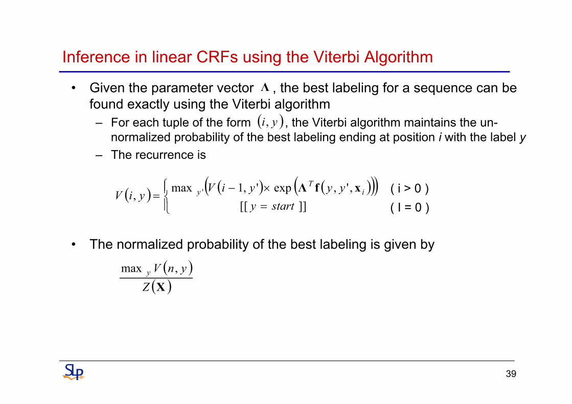
Inference in linear CRFs using the Viterbi Algorithm

• Given the parameter vector , the best labeling for a sequence can be found exactly using the Viterbi algorithm– For each tuple of the form , the Viterbi algorithm maintains the un-

normalized probability of the best labeling ending at position i with the label y– The recurrence is

• The normalized probability of the best labeling is given by

Λ

( ) ( ) ( )( )( )⎪⎩

⎪⎨⎧

=×−

=]][[

,',exp',1max, '

startyyyyiVyiV i

Ty xfΛ

( )yi,

( i > 0 )( I = 0 )

( )( )XZ

ynVy ,max

40

Training (Parameter Estimation)

• The various methods used to train CRFs differ mainly in the objective function they try to optimize– Penalized log-likelihood criteria– Voted perceptron– Pseudo log-likelihood– Margin maximization– Gradient tree boosting– Logarithmic pooling– and so on …

41

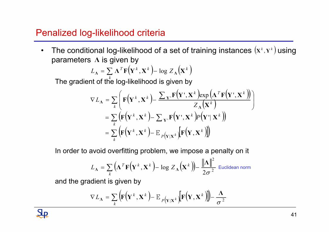
Penalized log-likelihood criteria

• The conditional log-likelihood of a set of training instances using parameters is given by

The gradient of the log-likelihood is given by

In order to avoid overfitting problem, we impose a penalty on it

and the gradient is given by

Λ( ) ( )∑ −=

k

kkkT ZL XXYFΛ ΛΛ log,

( )kk YX ,

( ) ( ) ( )( )( )

( ) ( ) ( )( )( ) ( ) ( )[ ]( )∑

∑ ∑

∑ ∑

−=

−=

⎟⎟⎠

⎞⎜⎜⎝

⎛−=∇

k

kP

kkk

kkkk

kk

kTkkk

k

P

ZL

XYFXYF

XYXYFXYF

XXYFΛXYF

XYF

XY

Y

Λ

YΛ

,,

|',',

,'exp,',

|

'

'

Ｅ

( ) ( )( ) 2

2

2log,

σΛ

XXYFΛ ΛΛ −−= ∑k

kkkT ZL Euclidean norm

( ) ( ) ( )[ ]( ) 2|,,

σΛXYFXYF

XYΛ −−=∇ ∑k

kP

kkkL Ｅ

42

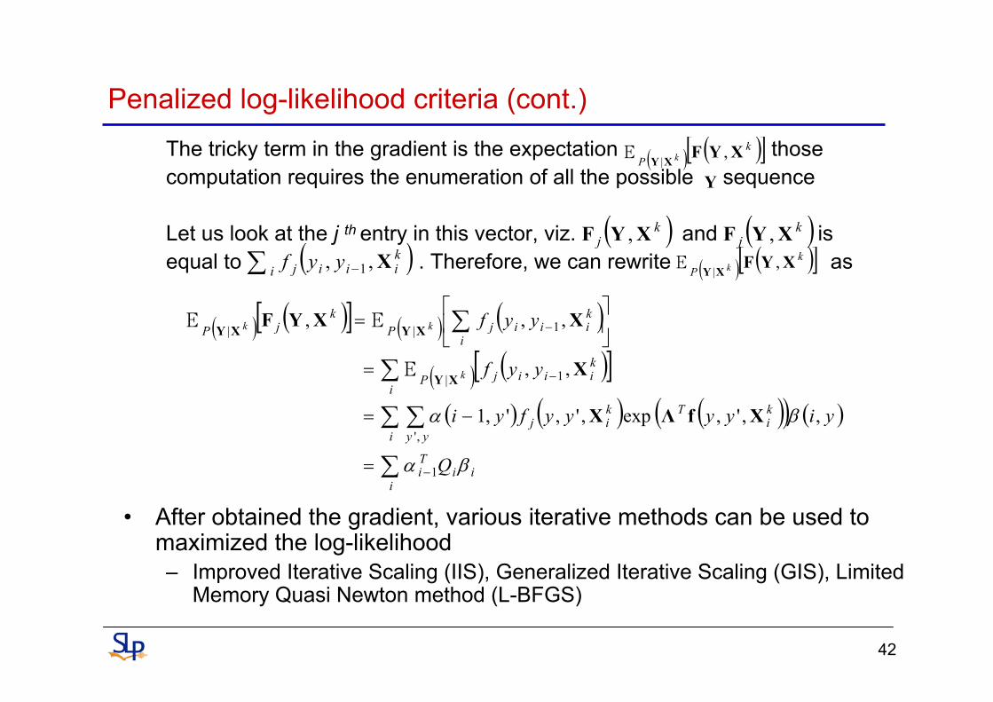
Penalized log-likelihood criteria (cont.)

The tricky term in the gradient is the expectation those computation requires the enumeration of all the possible sequence

Let us look at the j th entry in this vector, viz. and is equal to . Therefore, we can rewrite as

• After obtained the gradient, various iterative methods can be used to maximized the log-likelihood– Improved Iterative Scaling (IIS), Generalized Iterative Scaling (GIS), Limited

Memory Quasi Newton method (L-BFGS)

( ) ( )[ ]kP k XYF

XY,

|Ｅ

Y

( )kj XYF , ( )kj XYF ,( )∑ −i

kiiij yyf X,, 1 ( ) ( )[ ]k

P k XYFXY

,|

Ｅ

( ) ( )[ ] ( ) ( )

( ) ( )[ ]( ) ( ) ( )( ) ( )

∑

∑ ∑

∑

∑

−

−

−

=

−=

=

⎥⎦

⎤⎢⎣

⎡=

iii

Ti

i

ki

T

yy

kij

i

kiiijP

i

kiiijP

kjP

Q

yiyyyyfyi

yyf

yyf

k

kk

βα

βα

1

,'

1|

1||

,,',exp,',',1

,,

,,,

XfΛX

X

XXYF

XY

XYXY

Ｅ

ＥＥ

43

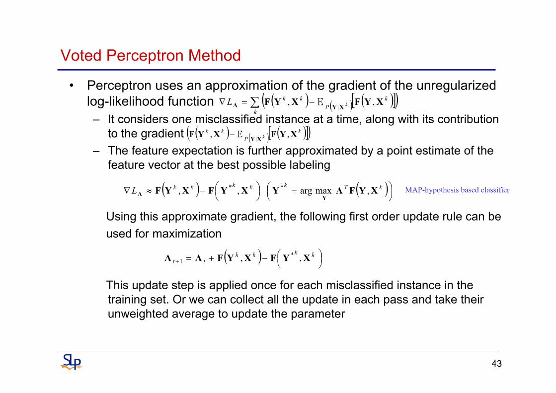
Voted Perceptron Method

• Perceptron uses an approximation of the gradient of the unregularizedlog-likelihood function– It considers one misclassified instance at a time, along with its contribution

to the gradient– The feature expectation is further approximated by a point estimate of the

feature vector at the best possible labeling

Using this approximate gradient, the following first order update rule can be used for maximization

This update step is applied once for each misclassified instance in the training set. Or we can collect all the update in each pass and take their unweighted average to update the parameter

( ) ( ) ( )[ ]( )∑ −=∇k

kP

kkkL XYFXYF

XYΛ ,,|

Ｅ

( ) ( ) ( )[ ]( )kP

kkk XYFXYF

XY,,

|Ｅ−

( ) ( )⎟⎠⎞⎜

⎝⎛ =⎟

⎠⎞⎜

⎝⎛−≈∇ kTkkkkkL XYFΛYXYFXYF

YΛ ,maxarg ,, ** MAP-hypothesis based classifier

( ) ⎟⎠⎞⎜

⎝⎛−+=+

kkkktt XYFXYFΛΛ ,, *

1

44

Pseudo log-likelihood

• In many scenarios, we are willing to assign different error values to different labeling– It makes senses to maximize the marginal distributions instead of

– This objective is called the pseudo-likelihood and for the case of linear CRFs, it is given by

( )( )( )

( )∑ ∑ ∑

∑∑

= =

=

=

=

k

T

t yyk

kTk

T

t

kkt

ktt

Z

yPL

1 :

1

,explog

,|log

y Λ

Λ

XXyFΛ

ΛX

( )kktyP X|

( )kkP XY |

45

• Semi-Markov CRFs– It is still in the realm of first-order Markovian dependence, but the different is

the label depend only on segment feature and the label of previous segment• Instead of assigning labels to each position, assign labels to segments

• Skip-Chain CRFs– A conditional model that collectively segments a document into mentions

and classifies the mentions by entity type

Other types of CRFs

Semi-Markov CRFs

A B CSkip-chain CRFs

A A B

46

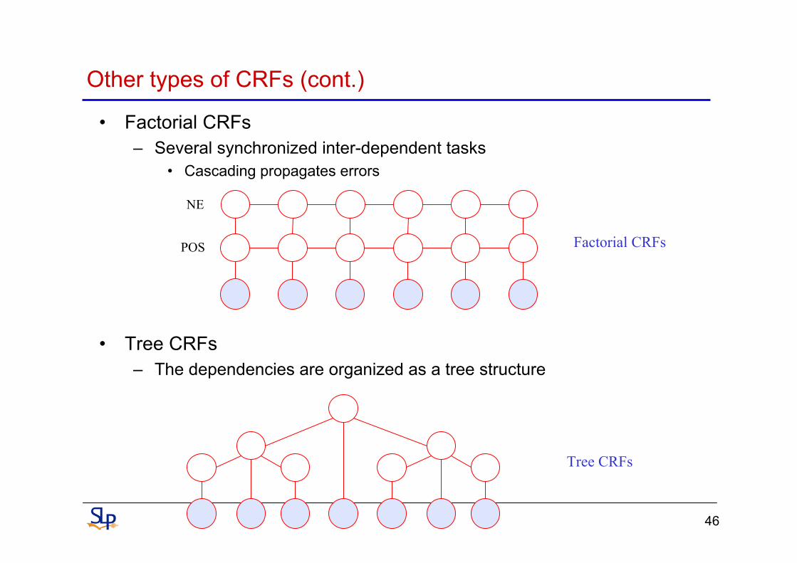
Other types of CRFs (cont.)

• Factorial CRFs– Several synchronized inter-dependent tasks

• Cascading propagates errors

• Tree CRFs– The dependencies are organized as a tree structure

Factorial CRFsPOS

NE

Tree CRFs

47

Conclusions

• Conditional Random Fields offer a unique combination of properties– discriminatively trained models for sequence segmentation and labeling– combination of arbitrary and overlapping observation features from both

the past and future– efficient training and decoding based on dynamic programming for a

simple chain graph– parameter estimation guaranteed to find the global optimum

• Possible Future work?– Efficient training approach ??– Efficient Feature Induction ??– Constrained Inferencing ??– Different topology ??

48

Reference• Lafferty, J., McCallum, A., Pereira, F., “Conditional random fields: Probabilistic models for segmenting

and labeling sequence data,” In: Proc. 18th International Conf. on Machine Learning, Morgan Kaufmann, San Francisco, CA (2001) 282–289.

• Rahul Gupta, “Conditional Random Fields,” Dept. of Computer Science and Engg., IIT Bombay, India. Document available from http://www.it.iitb.ac.in/~grahul/main.pdf

• Sutton, C., McCallum, A., “An Introduction to Conditional Random Fields for Relational Learning,”Introduction to Statistical Relational Learning, MIT Press. 2007. Document available from http://www.cs.berkeley.edu/~casutton/publications/crf-tutorial.pdf

• Mitchell, T. M., “Machine Learning,” McGraw Hill, 1997. Document available from http://www.cs.cmu.edu/~tom/mlbook.html

• Bishop, C. M., “Pattern Recognition and Machine Learning,” Springer, 2006• Bishop, C. M., “Graphical Models and Variational Methods,” video lecture, Machine Learning Summer

School 2004. Available from http://videolectures.net/mlss04_bishop_gmvm/• Ghahramani, Z., “Graphical models,” video lecture, EPSRC Winter School in Mathematics for Data

Modelling, 2008. Available from http://videolectures.net/epsrcws08_ghahramani_gm/• Roweis, S., “Machine Learning, Probability and Graphical Models,” video lecture, Machine Learning

Summer School 2006, Available from http://videolectures.net/mlss06tw_roweis_mlpgm/