Embed Size (px)
Citation preview
Graphical Interactive Simulation InputModeling with Bivariate E%zier Distributions
MARY ANN FLANIGAN WAGNER
Purdue University
and
JAMES R. WILSON
North Carolina State University
A graphical interactive technique for modeling bivariate simulation inputs is based on a family ofcontinuous univariate and bivariate probability distributions with bounded support that aredescribed by B6zier curves and surfaces, respectively. This family of distributions has a natural,extensible parameterization so that all parameters have a meaningful interpretation; and thecomplete family is capable of accurately representing an unlimited variety of shapes for marginaldistributions together with many common types of blvariate stochastic dependence. This ap-proach to simulation input modeling is implemented in a Windows-based software system calledPmw-probabilistic Input Modeling Environment. Several examples illustrate the applicationof PRIME to subjective and data-driven estimation of bivariate distributions representing simula-tion inputs.
Categories and Subject Descriptors: G.3 [Mathematics of Computing]: Probability and Statis-I,ics-staz%tical software; 1.6.5 [Simulation aml Modeling]: Model Development—modelingm eth odo[ogtes; 1.6.7 [Simulation and Modeling]: Simulation Support Systems—en Luronmen ts
General Terms: Algorithms, Design, Theory
Additional Key Words and Phrases: Graphical interactive distribution fitting
1. INTRO13LKHION
One of the central problems in the design and construction of stochastic
simulation experiments is the selection of valid input models—that is,
This work was partially supported by a David Ross Grant from the Purdue Research Foundationand by NSF grant DIvE-87 17799. A preliminary version of this work was presented at the 1994Winter Simulation Conference, which was held December 11–14, 1994, in Ch-lando,Florida, andwas sponsored by ASA, ACM, IEEE, IIE, NIST, ORSA, TIMS, and SCS.Authors’ addresses: Mary Ann Flanigan Wagner, Boeing Information Services, 7990 BoeingCourt, Vienna, VA 22183-7000: email: (maf lani@w~. ecld; James ~. Wilso% Department ofIndustrial Engineering, North Carolina State University, Raleigh, NC 27695-7906; email:(]wllsOn@:eOs .ncsu. edu).
Permission to make digital/hard copy of all or part of this material without fee is grantedprovided that the copies are not made or distributed for profit or commercial advantage. theACM copyright/server notice, the title of the publication. and its date appear, and notice is giventhat copying is by permission of the Association for Computing Machinery, Inc. (ACM). To COPY
otherwise, to republish, to post on servers, or to redistribute to lists requires prior specificpermission and/or a fee.01995 ACM 1049-3301/95/0700-0163 $03.50
ACM Transactions on Modehng and Computer Simulation, Vol. 5, No. 3, July 1995, Pages 163-189.
164 . M A. Flanigan Wagner and J R, Wilson
probability distributions that accurately mimic the behavior of the random
input processes driving the system. In many applications, it is critical not
only to capture the shape of the marginal distribution of each major input
random variable but also to accurately represent the stochastic dependencies
between those variates [Lewis and Orav 1989, p. 291]. For example, in
modeling the arrival streams of liver-transplant donors and patients for the
UNOS Liver Allocation Model [Pritsker et al. 1995], initially we had to model
the stochastic dependence between the age and weight of each new arrival;
and ultimately we had to expand our stochastic model to include the sex and
blood type of each new arrival.
Although many practitioners appreciate the need for valid models of multi-
variate simulation inputs, they lack effective and widely available took for
building such input models. Stanfield and Wilson [1993] developed a tech-
nique for fitting a multivariate distribution when the correlation matrix and
the first four moments for each marginal distribution have been specified or
estimated by the user. Because the fitted joint distribution is built from
univariate marginals belonging to the Johnson translation system [Johnson
1949a; Swain et al. 1988], the multivariate input-modeling technique of
Stanfield and Wilson has substantial flexibility. Unfortunately, the fitted
joint distribution does not belong to the multivariate Johnson translation
system [Johnson 1949b; Johnson 1987]; moreover, the corresponding condi-
tional distributions do not belong to the Johnson system—and this lack of
“closure” makes it impossible to obtain convenient closed-form expressions for
the conditional distributions that naturally arise in many applications. Al-
though DeBrota et al. [1989] developed a graphical interactive software
system that enables the user to edit (manipulate) univariate bounded John-
son distributions, it is unclear that a similar tool could be based on the
multivariate distribution-fitting procedure of Stanfield and Wilson.
Other approaches to multivariate input modeling can be based on TES
(Transform-Expand-Sample) processes [Jagerman and Melamed 1992a,1992b; Melamed et al. 1992] and ARTA (AutoRegressive To Anything) pro-
cesses [Cario and Nelson 1995]. Both methodologies enable the user to specify
the autocorrelation function out to an arbitrary lag for a univariate stochastic
process with a user-specified marginal distribution, but ARTA processes seem
to be substantially easier to use. Unfortunately, the conditional distributions
associated with TES and ARTA processes do not appear to possess any
advantages in analytical or numerical tractability when compared to multi-
variate processes based on the Johnson translation system. Software pack-
ages for fitting TES and ARTA processes are not widely available at thepresent time.
In this article we extend the univariate input-modeling methodology of
Wagner and Wilson [1993, 1995] to handle continuous bivariate populations
with bounded support, and we present a flexible, interactive, graphical
technique for modeling a broad range of bivariate simulation inputs. We
employ B6zier surfaces as the parametric form for representing the distribu-
tion function of continuous bivariate random vectors that are to be randomly
sampled in a simulation experiment, and we show that the corresponding
ACM Transactions on Modeling and Computer Simulation, Vol. 5, No 3, July 1995.
Simulation Input Modeling . 165
marginal and conditional distributions belong to the original family of uni-
variate B6zier distributions. We implemented this methodology in a Microsoft
Windows-based software system called PRIME —l?Robabilistic Input Modeling
Environment. A public-domain version of the software is available upon
request.
The remainder of this article is organized as follows. In Section 2 we
summarize the main properties of univariate B6zier distributions that are
relevant for our development of bivariate B6zier distributions, and we estab-
lish some basic notation that is used throughout the paper. In Section 3 we
detail our methodology for constructing, manipulating, and sampling bivari-
ate B6zier distributions as well as the associated marginal and conditional
univariate B6zier distributions. In Section 4 we describe the implementation
of this methodology in PRIME, including techniques for interactively fitting
bivariate simulation input models using subjective information (expert opin-
ion) or sample data. In Section 5 we present some examples illustrating the
diversity of bivariate distributions that can be modeled using this methodol-
ogy. Finally, in Section 6 we summarize the main contributions of this work,
and we make recommendations for future research. Although this paper is
based on Flanigan [1993], some of our results were also presented in Wagner
and Wilson [1994].
2. OVERVIEW OF UNIVARIATE BEZIER DISTRIBUTIONS
2.1 Definition of B4zier Curves
In many applications of computer graphics, a B&ier curve is used to approxi-
mate a smooth (continuously differentiable) univariate function on a bounded
interval by forcing the B6zier curve to pass in the vicinity of selected control
points {p, = (x,, Z,)T: i = O, 1,..., n}. (Throughout this paper, all vectors will
be column vectors unless otherwise stated; and the reman superscript T will
denote the transpose of a vector or matrix so that each control point is
understood to be a column vector.) A B6zier curve of degree n with control
points {pO, pi,... , P.} is given parametrically by
P(t) = [Pz(t; n,x), PZ(t; n,z)lT = ~B.,,(t)p, for t ~ [0,11, (1)~=o
where x - (X O, Xl,..., x~)T and z = (Z O, ZI, ..., z~)T, and where the blend-
ing function B .,,(t) k the Bernstein polynomial
[
n!
Bn,l(t) ~ i!(n – i)!tl(l – t)n-’ , fort =[0, l] and i= O,l,..., n,
o, otherwise.
(2)
B6zier curves have certain characteristics that are particularly important for
graphically based approximation of functions [Farin 1990]:
(a) A B6zier curve exactly interpolates its initial and final control points; thismeans that the curve will pass through these control points.
ACM Transactions on Modeling and Computer Simulation, Vol 5, No. 3, July 1995.
166 . M. A. Flanlgan Wagner and J. R. Wilson
(b) A B6zier curve is edited under global control; this means that any changein the location of a control point affects the shape of the entire curve.
In the definition (a) of the B6zier curve {P(t): t = [0, 1]},notice that for
each t G [0, 1], we have E;.. 1?.,, ( t)= 1 because the ith Bernstein polyno-
mial B. ,( t ) can be interpreted as the binomial probability of i successes in n
independent trials with success probability t on each trial; thus the B&zier
curve traced by P(t) for all t G [0, 1] lies in the convex hull of the control
points {p,: i = 0,1, ..., n}. Although B6zier curves are edited under global
control, the effect of the ith control point p, on the shape of the curve is
greatest at the value t = i/n for the parameter t. In particular, as t in-
creases from O to 1, the weight B., O(t ) of the initial control point PO
decreases from 1 to O and the weight B .,.( t) of the final control point pn
increases from O to 1 in the overall weighted average (convex combination) of
control points that determines the current location P(t) on the B&zier curve.
Thus the control points act like “magnets”; and the “magnetic attraction”
exerted on the B6zier curve {P(t): t E [0, I]} by the ith control point p, is
strongest at the value t = i/n for the parameter t so that the corresponding
point P(t) on the curve is “in the vicinity” of p,. If the weight (magnetic
attraction) of a control point is 1, then the B6zier curve is forced to pass
through that control point exactly.
2.2 Formulation of Univariate Bezler Probability Distributions
In this section we summarize briefly some key properties of univariate B6zier
distributions. For a detailed development of these properties, see Wagner and
Wilson [ 1993, 1995]. Given a continuous random variable X with bounded
support [ x*, x”] and unknown cumulative distribution function (c.d.f.) Fx (. ),
we can approximate Fx(. ) arbitrarily closely by a Biizier curve of the form (1)
with sufficiently high degree n, where
x(t) = ~B@r,~=o
1
for all t G [0,1].
Fy[x(t)] = ~ B~,, (t)z,~=fJ
(3)
If Fx(.) is given parametrically by Equation (3), then the correspondingprobability density function (p.d.f.) &-(.) is given parametrically by
x(t) = i Bn,, (t)x,l=(J
n–1
/
n–1 Ifor all t S [0,1], (4)
f’x[x(t)l = z Bn-l, z(t)Azt Z B..l,, (t) Ax,~=o ~=o
ACM Transactions on Modeling and Computer .%mulatlon, Vol 5, No. 3, July 1995
Simulation Input Modeling . 167
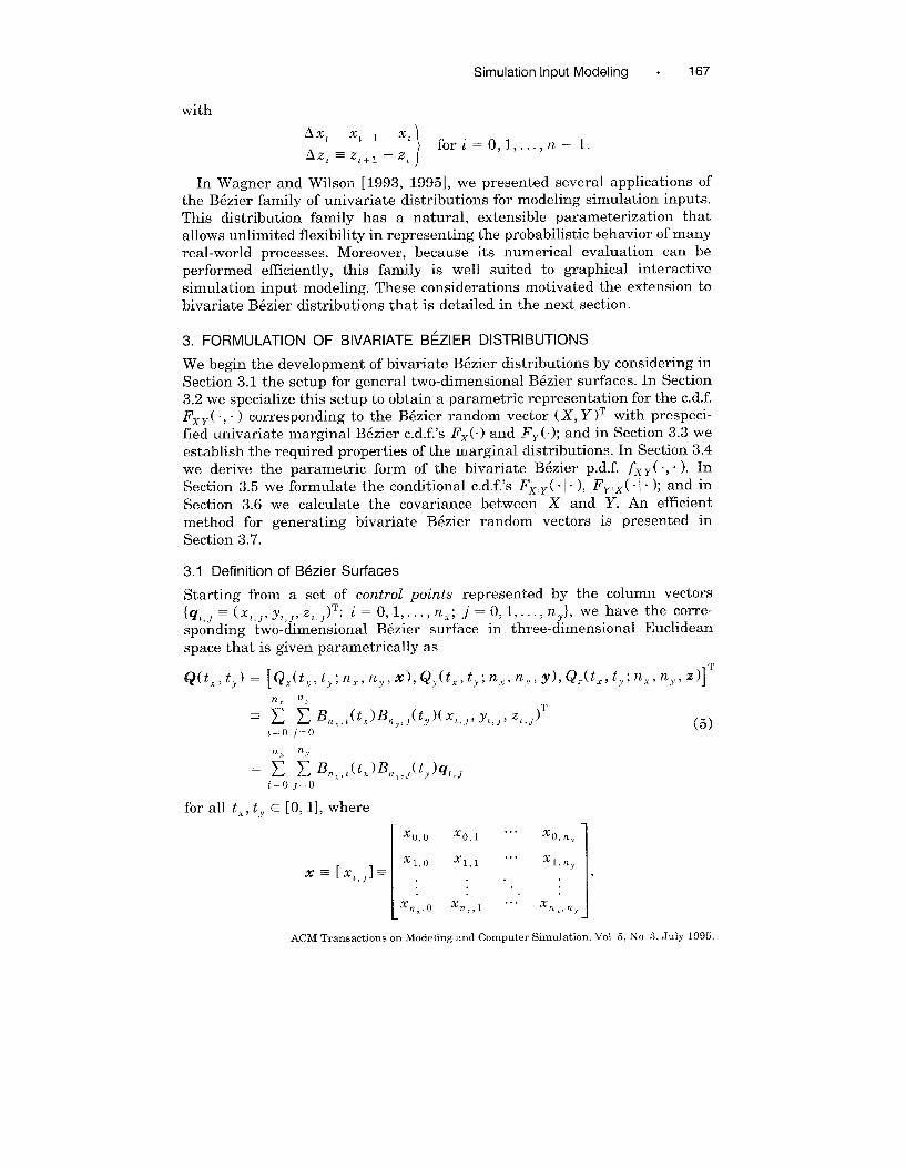
with
Axl =Xl+l ‘Xl
Azt =Zl+l ‘Zl)
fori=O, l,..., n–l.
In Wagner and Wilson [1993, 1995], we presented several applications of
the B6zier family of univariate distributions for modeling simulation inputs.
This distribution family has a natural, extensible parameterization that
allows unlimited flexibility in representing the probabilistic behavior of many
real-world processes. Moreover, because its numerical evaluation can be
performed efficiently, this family is well suited to graphical interactive
simulation input modeling. These considerations motivated the extension to
bivariate B6zier distributions that is detailed in the next section.
3. FORMULATION OF BIVARIATE BEZIER DISTRIBUTIONS
We begin the development of bivariate B6zier distributions by considering in
Section 3.1 the setup for general two-dimensional B6zier surfaces. In Section
3.2 we specialize this setup to obtain a parametric representation for the c.d.f.
FXY(”, ‘ ) corresponding to the B6zier random vector (X, Y )T with prespeci-
fied univariate marginal B6zier c.d.f.’s F’x(”) and FY( “); and in Section 3.3 we
establish the required properties of the marginal distributions. In Section 3.4
we derive the parametric form of the bivariate Bi$zier p.d.f. fx y (”, ” ). In
Section 3.5 we formulate the conditional c.d.f.’s Fxly(” I” ), Fy ,x(”\. ); and inSection 3.6 we calculate the covariance between X and Y. An efficient
method for generating bivariate B6zier random vectors is presented in
Section 3.7.
3.1 Definition of Bezier Surfaces
Starting from a set of control points represented by the column vectors
{qL, J - (~1, j, Y1,J, ZL. J)T: i = 0,1,.., ~x; ~ = 0, 1)7 ny}, We have the Corre-
sponding two-dimensional B6zier surface in three-dimensional Euclidean
space that is given parametrically as
Q(tx, ty) = [Qx(tx, ty; nZ, ny, x), Qy(tx, ty; nx, nJ, y), QZ(tx, ty; nx, n,y, z)]T
= ~ ; Bnt, L(tx)Bny,,(ty)( xL,,, y,,,, z,,j)T~=oj=o
= ; t Bni, t(tl)Bn,,,(ty)qL,,2=OJ=0
(5)
for all tx, ty G [0, 1], where
‘“[XLJ]=FO:l :]
ACM Transactions on Modeling and Computer Simulation, Vol 5, No 3, July 1995.
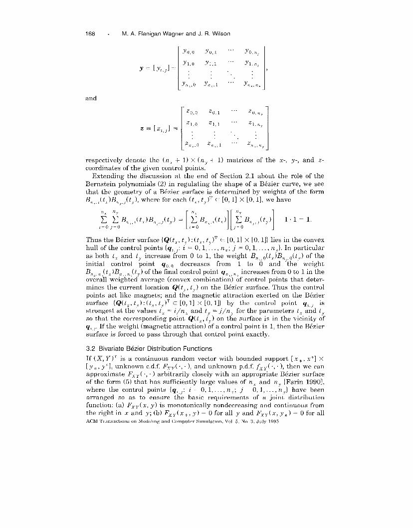
168 . M. A. Flanigan Wagner and J. R, Wilson
[Yo, o Yo,l ““” 3’0, nv
Yl, o Yl,l ““” Yl, nyY=[yt, ll= . , . .
\ Ynz,o Yn=,l ““” Ynz,rz,L
and
Z=[z,j]=
respectively denote the ( n ~ +
~o, o 2.,1 . . . ‘O, n Y
~1, o 21,1 ““” ‘l, nY
z “ i?n ~ ‘-. Zn,,n., ., nY
>
1
1) x (n, + 1) matrices of the x-, y-, and z-
coordinates of the given control points:
Extending the discussion at the end of Section 2.1 about the role of theBernstein polynomials (2) in regulating the shape of a B6zier curve, we see
that the geometry of a B6zier surface is determined by weights of the form
B~,,,(t, )BmY,~(tY), where for each (tX, tY)T = [0, 1] X [0, 1], we have
~ ~ B~r,,(tX)BZ=OJ=O
.yj(t)=[~OBn,(,)][}oB.,,(y)]=ll=l
Thus the B&zier surface {Q(tX, ty) : (t,, ty)T ● [0, 1] X [0, 1]} lies in the convex
hull of the control points {q,, ~: z = O, 1,..., nX; j = O, 1,..., nY}. In particular
as both tx and ty increase from O to 1, the weight B.,, o(tX)B~Y, 0( t,) of the
initial control point qo, o decreases from 1 to O and the- weightB ~z2~JtX)B .,, .JtY) of the final control point qnt,,, increases from O to 1 in theoverall weighted average (convex combination) of control points that deter-
mines the current location Q(tx, ty ) on the B6zier surface. Thus the control
points act like magnets; and the magnetic attraction exerted on the B6ziersurface {Q(tx, ty) : (tx, ty)T G [0, I] X [0, I]} by the control point qL, J is
strongest at the values t,= i/n Z and ty= J“/nY for the parameters tx and tY
so that the corresponding point Q( tx,ty) on the surface is in the vicinity of
q,,,. If the weight (magnetic attraction) of a control point is 1, then the B~ziersurface is forced to pass through that control point exactly.
3.2 Bivariate Bezier Distribution Functions
If (X, Y )’ is a continuous random vector with bounded support [.x*, x*] x
[Y., y’], unknown c.d.f. F.~Y(”, “ ), and unknown p.d.f. &Y(., . ), then we canapproximate Fry (., . ) arbitrarily closely with an appropriate B6zier surfaceof the form (5) that has sufficiently large values of n ~ and n ~ [Farin 1990],
where the control points {q,, J: i = O, 1,....nX; j = O, 1,....ny} have been
arranged so as to ensure the basic requirements of a joint distribution
function: (a) FAY~,( x, y) is monotonically nondecreasing and continuous from
the right in x and y; (b) FXY(XX, y) = O for all y and FXY(X, y*) = O for all
ACM TransactIons on Modehng and Computer S1mulatlon, Vol. 5, NCJ 3, July 1995
Simulahon Input Modeling . 169
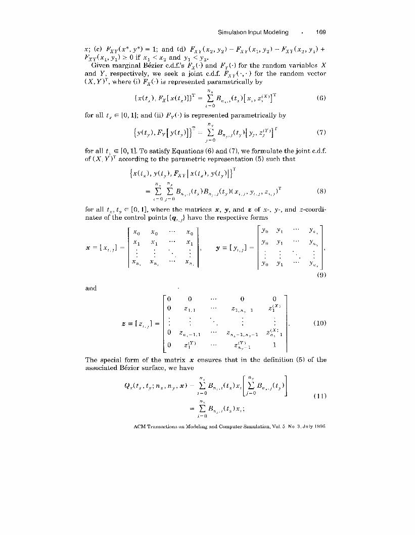
x; (c) FXY(X*, y*) = 1; and (d) FXY(ZZ, Yz) – FXY(XI, Y2) – Fxy(xz, Yl) +
FXY(XI, yl) >0 if xl < X2 and YI < Yz.Given marginal I%zier c.d.f.’s Fx(.) and FY(. ) for the random variables X
and Y, respectively, we seek a joint c.d.f. Fx Y(., “ ) for the random vector
(X, Y)T, where (i) Fx(”) is represented parametrically by
{x(tJ, Fx[x(tX)]}T ===~ BJtJ[xz, @]T~=()
(6)
for all tX ● [0, 1]; and (ii) FY(.) is represented parametrically by
{y(tY), FY[y(ty)]}T = ~ B#y)[yJ, Z;Y’]T (7)J=()
for all tY ● [0, 1]. To satisfy Equations (6) and (7), we formulate the joint c.d.f.
of ( X, Y )T according to the parametric representation (5) such that
{x(tJ,y(tY),Fxy [x(tX),y(tJ]}T
= ~ : Bnl,z(tx)Bn,,,(ty)(x,,,,y,,,, z,>,)T (8)~=OJ=o
for all tz, ty E [0, 1], where the matrices ~, y, and z of x-, y-, and z-coordi-
nates of the control points {q,, ~} have the respective forms
[X. X. ““” X.
, 1Y(l Y1 ““” Yn,
Yo Y1 ““” Yn,Y=[Y,, JI= . . . 7
. .
. . . .Yo Y1 ““” Yn,
(9)
and
[ ~
00
0 ‘Z1,l
Z=[z,, )l = : :
. . . 0 0
.. .‘1, n>–1
(x)z~
~ ‘1
. . (lo)
Oz ll– 1,1 ““”~:x~ ~
Zn –1,7L–1 ,t
[o (Y) . . .
z~Z(Y)
nj–l 11
The special form of the matrix ~ ensures that in the definition (5) of the
associated B6zier surface, we have
n,
ACM Transactions on Modeling and Computer Simulation, Vol. 5. No. 3, July 1995
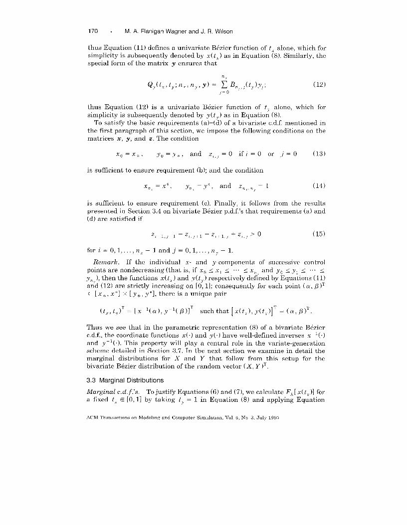
170 . M. A. Flanigan Wagner and J. R. Wilson
thus Equation (11) defines a univariate B6zier function of tx alone, which for
simplicity is subsequently denoted by x( t,)as in Equation (8). Similarly, the
special form of the matrix y ensures that
Qy(t,,ty;n.,n,,y) = f Bny,,(ty)y,; (12)~=o
thus Equation ( 12) is a univariate B6zier function of t,Y alone, which for
simplicity is subsequently denoted by y(tY ) as in Equation (8).
To satisfy the basic requirements (a)–(d) of a bivariate c.d.f, mentioned in
the first paragraph of this section, we impose the following conditions on the
matrices x, y, and z. The condition
x(j =x*, YO =Y. , and z,. j =0 ifi=O or j=O (13)
is sufficient to ensure requirement (b); and the condition
x =X*, Y., =.v*, and z,,,,., = 1 (14)~i
is sufficient to ensure requirement (c). Finally, it follows from the results
presented in Section 3.4 on bivariate B6zier p.d.f.’s that requirements (a) and
(d) are satisfied if
+2 ,J>oZL+l,J+l —~l, j+l — ~t+l,j (15)
fori=O, l,..., nlandj=O, l, l,... ,nY–l.
Remark. If the individual x- and y-components of successive control
points are nondecreasing (that is, if XO < xl < ““” < x., and yO s yl < “.” <
y.,), then the functions x( t,)and y(tY) respectively defined by Equations (11)and (12) are strictly increasing on [0, 1]; consequently for each point (a, ~ )T~ [X*, x*] x [y*, y*], there is a unique pair
(tl,tJT = [x-’(cd, y-’3)]T]T such that [x(tI), y(tY)]T = (CK, /3)T.
Thus we see that in the parametric representation (8) of a bivariate B4zier
c.d.f., the coordinate functions x(. ) and y(. ) have well-defined inverses x-1(. )
and y-1 ( .). This property will play a central role in the variate-generationscheme detailed in Section 3.7. In the next section we examine in detail the
marginal distributions for X and Y that follow from this setup for the
bivariate B&zier distribution of the random vector (X, Y )T.
3.3 Marginal Distributions
Marginal cd. f.’s. To justify Equations (6) and (7), we calculate F.Y[ x( tx)]for
a fixed tX G [0, 1] by taking ty= 1 in Equation (8) and applying Equation
ACM TransactIons on Modeling and Computer Simulation, Vol. 5, No 3, July 1995
Simulation Input Modeling . 171
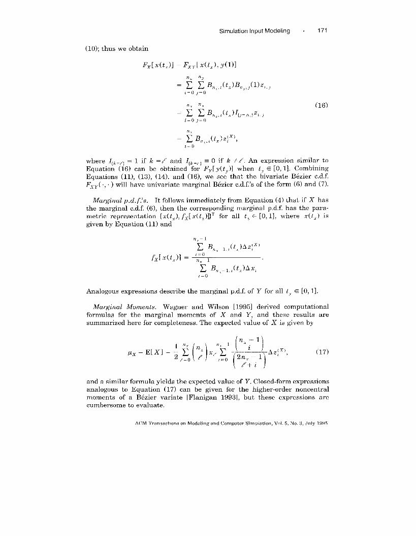
(10); thus we obtain
Fx[a?(tx)] = Fxy[x(tz), y(l)]
(16)
n,
where ]~h.~) - 1 if k = Y’ and Ifh.., - 0 if k #~. An expression similar toEquation (16) can be obtained for FY[ Y( tY )1 when tY ~ [0, 11. Combining
Equations (11), (13), (14), and (16), we see that the bivariate B6zier c.d.f.
FXY(., . ) will have univariate marginal B6zier c.d.f.’s of the form (6) and (7).
Marginal pd. f.’s. It follows immediately from Equation (4) that if X has
the marginal c.d.f. (6), then the corresponding marginal p.d.f. has the para-metric represe~tation {x(tX), fx[ x(tt)]}T for all tZ ~ [0, 11, where ~(tX) is
given by Equation (11) and
nx–l
~ B~,__l,,(tX)Az}x)
Analogous expressions describe the marginal p.d.f. of Y for all t-v G [0, 1].
Marginal Moments. Wagner and Wilson [1995] derived computational
formulas for the marginal moments of X and Y, and these results are
summarized here for completeness. The expected value of X is given by
and a similar formula yields the expected value of Y. Closed-form expressions
analogous to Equation (17) can be given for the higher-order noncentral
moments of a B6zier variate [Flanigan 1993], but these expressions arecumbersome to evaluate.
ACM TransactIons on Modeling and Computer Simulation, Vol. 5, No. 3, July 1995
172 . M. A. Flanigan Wagner and J R. Wilson
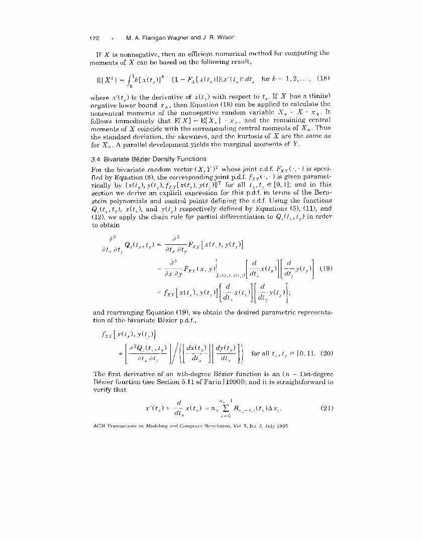
If X is nonnegative, then an efficient numerical method for computing the
moments of X can be based on the following result,
E[X~] = /&(t X)] ‘-’{1 –~y[x(t i)]}lx’(tx)ld. fork = 1,2,, (18)o
where x’( t,) is the derivative of x( t.) with respect to t..If X has a (finite)
negative lower bound x*, then Equation (18) can be applied to calculate the
noncentral moments of the nonnegative random variable Xx - X – x ~. It
follows immediately that E[ Xl = E[ Xx 1 + x,,, and the remaining central
moments of X coincide with the corresponding central moments of XX. Thus
the standard deviation, the skewness, and the kurtosis of X are the same as
for X*. A parallel development yields the marginal moments of Y.
3.4 Bhariate Bezier Density Functions
F’or the bivariate random vector (X, Y )T whose joint c.d.f. Fx y (., “ ) is speci-
fied by Equation (8), the corresponding joint p.d.f. fxy ( ~, “ ) is given paramet-
rically by {x(tX), y(tj), fxy[x(t, ), y(tv)l}T for all ti, tY ~ [0, 11; and in this
section we derive an explicit expression for this p.d.f. in terms of the Bern-
stein polynomials and control points defining the c.d.f. Using the functions
Qz(tx, ty ), x(t, ), and y(t,) respectively defined by Equations (5), (11), and(12), we apply the chain rule for partial differentiation to Q,( t.,ty) in orderto obtain
~i
Qz(~x,ty) = ~td;tFxy[x(t.t), Y(ty)]dtxdt
Y x y
and rearranging Equation (19), we obtain the desired parametric representa-
tion of the bivariate B6zier p.d.f.,
The first derivative of an nth-degree B6zier function is an (n – l)st-deg-ee
B6zier function (see Section 5.11 of Farin [1990]); and it is straightforward to
verify that
(21)
ACM TransactIons cm Modeling and Computer S]mulatlon, Vol 5, No 3, July 1995
Simulation Input Modellng . 173
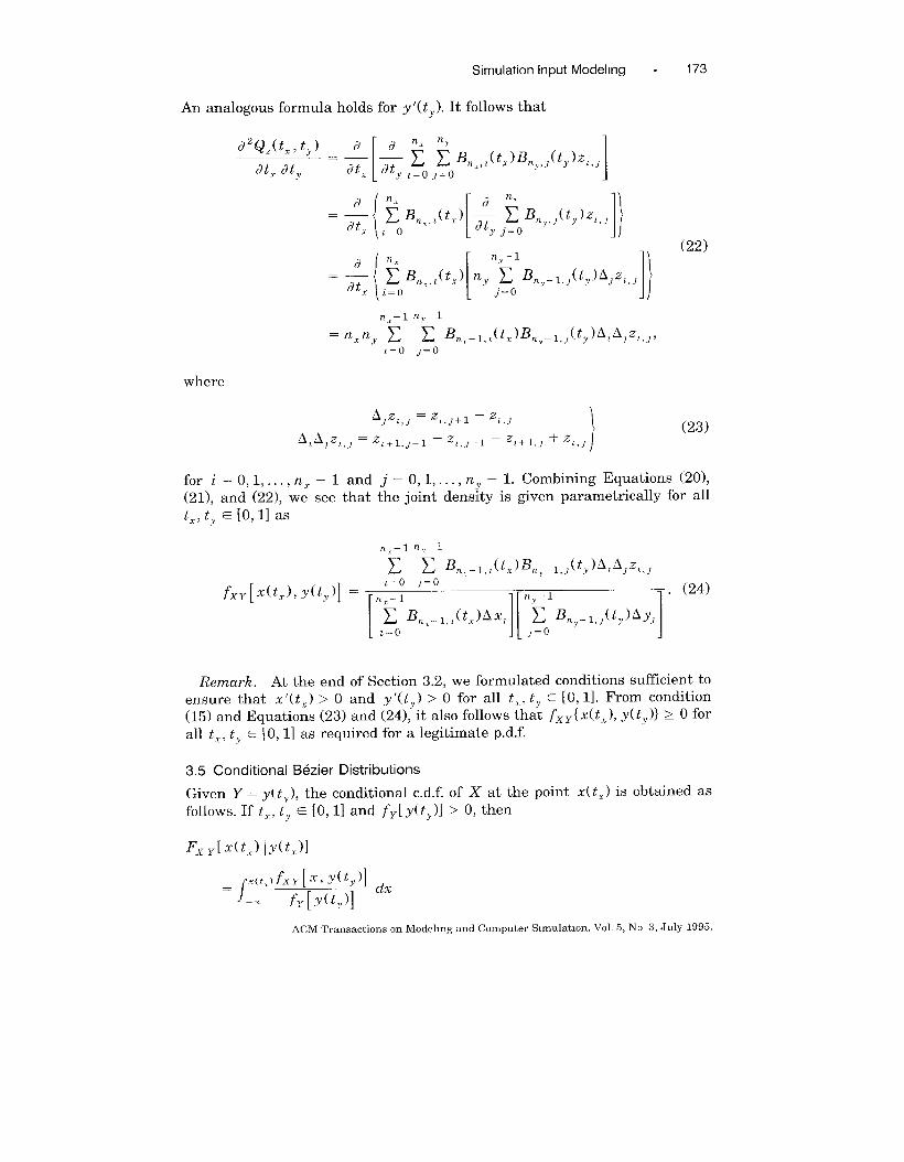
An analogous formula holds for y ‘(tY ). It follows that
where
for i = O, 1,..., rzX – 1 and j = O, 1,..., nY – L Combining Equations (20),
(21), and (22), we see that the joint density is given parametrically for alltx, t, G [0, 1] as
Remark. At the end of Section 3.2, we formulated conditions sufficient to
ensure that x ‘(tX) > 0 and y ‘(ty) > 0 for all t,, ty G [0, 1]. From condition
(15) and Equations (23) and (24), it also follows that fxY{ x(tl ), Y( t,)} >0 for
all tX, tY ● [0, 1] as required for a legitimate p.d.f.
3.5 Conditional B6zier Distributions
Given Y = y(t, ), the conditional c.d.f. of X at the point x( tx ) is obtained as
follows. If tX, t, G [0, 11 and fY[y(ty)l >0, then
Fxly[x(tx)Iy(t.)1
ACM Transactions on Modeling and Computer Slmulat,on, Vol. 5, No 3, July 1995.
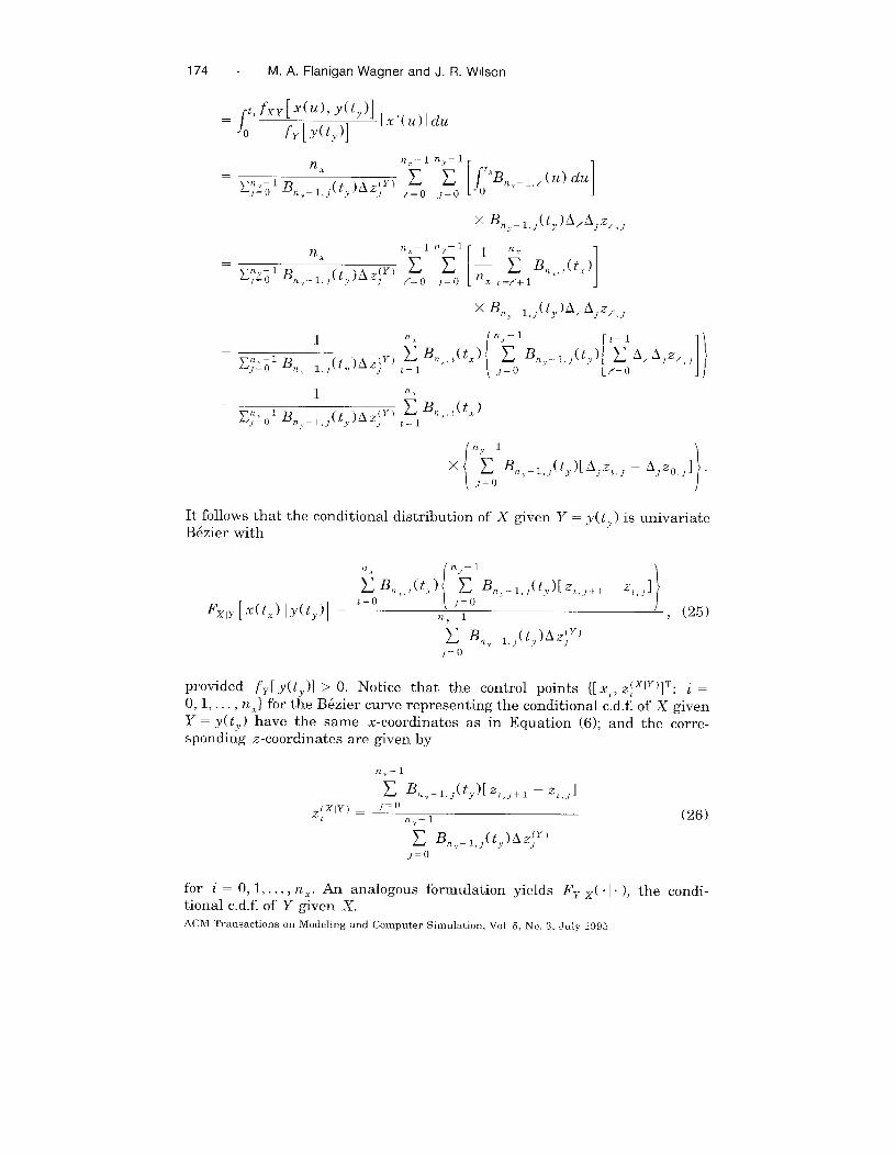
174 - M. A. Flanigan Wagner and J. R. Wilson
It follows that the conditional distribution of X given Y = y(tY ) is univariate
B6zier with
provided ~y[ y(tY’)] >0. Notice that the control points {[ x,, z~xlyJ]T: i =0, 1, . . . . nt} for the B&zier curve representing the conditional c.d.f. of X given
Y = y(t~ ) have the same x-coordinates as in Equation (6); and the corre-
sponding z-coordinates are given by
nv—l
Z 8Z-,,,(~yYZ,,,+I -z,,,]Z(XIY) = ,=0
[ nv—l (26)
for z = O, 1,... , n ~. An analogous formulation yields Fy ,x( . I ~), the condi-
tional c.d.f. of Y given X.
ACM Transactions on Modeling and Computer Simulation, Vol 5, No. 3, July 1995
Simulation Input Modeling . 175
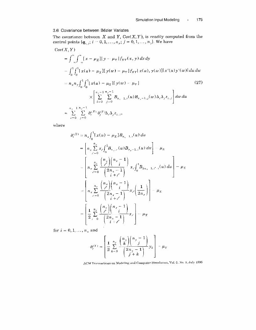
3.6 Covariance between Bezier Variates
The covariance between X and Y, Cov( X, Y ), is readily computed from the
control points {ql, ~; i = O, l,. ... nf; .j = O, l,. ... nY}. We have
COV(X, Y)
=/”/”[ x – pxl[y –pylfxy(~>Y)ci~clY—. —.
= nxny/l/l[ x(u) - I%yl[y(w) - Pyl (27)00
where
fori=O,l,..., nX and
ACM Transactions on Modeling and Computer Simulation, Vol. 5, No. 3, July 1995
176 . M. A. Flanigan Wagner and J. R. Wilson
forj=O, l,. ... rzY. Notice that the expected value E[ X] (respectively, E[ Y 1)
and the variance Var[ X ] (respectively, Var[ Y ]) are readily evaluated using
the computational formulas (17) and (18). Thus we can easily compute
Corr( X, Y ), the correlation between X and Y.
3.7 Generation of B6zier Vectors
The random vector (X, Y )T can be generated efficiently using a variant of the
method of conditional distributions that we call “ piecewise conditioning.” To
explain piecewise conditioning, we first summarize the conventional method
of conditional distributions.
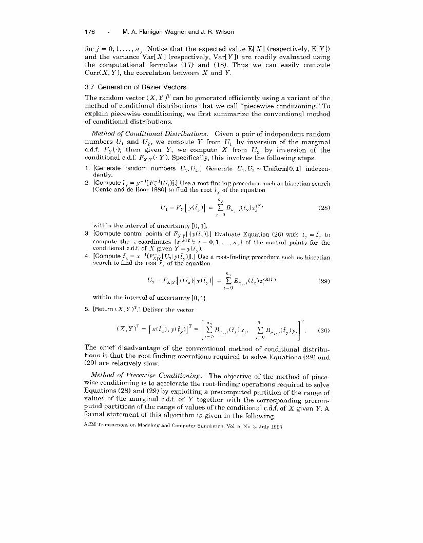
Method of Conditional Distributions. Given a pair of independent random
numbers UI and Uz, we compute Y from UI by inversion of the marginal
c.d.f. FY(. ); then given Y, we compute X from Uz by inversion of the~lY(.lY). Specifically, this involves the following steps.conditional c.d.f. F
1.
2.
3
4,
5.
[Generate random numbers Ul, Uz.] Generate Ul, Uz - Uniform[O, 1] indepen-dently.
[Compute Z, = Y- 1[F= l(U1)I.I Use a root-finding procedure such as bisection search[Conte and de Boor 1980] to find the root f, of the equation
q
U1 =FY[Y(~.y~] = ,;O%,,,WT (28)
within the interval of uncertainty [O, 1].
[@mPute control Points of F.YIY[ I Y( i,~l.1 Evaluate Equation (26) with t, = i, tocompute the z-coordinates {Z~z-lyl. ~ = O, I, . . . . ~ ~} of the control points for theconditional c.d.f. of X given Y = y(~}).
[Compute ~X= x-1 {F’~l~[ Uz IY( i, )]}.] Use a root-finding procedure such as bisectionsearch to find the root tx of the equation
u, = F.yly[x(il)ly(iy)] = ~ Bn,,, (ix)zy)Z=()
within the interval of uncertalnt y [0, 1].
[Return (X, Y )T.] Deliver the vector
(29)
[ IT
(X, Y)T= [x(i), y(iJ]T= fll,lx,l(;.t)x,,; Bny,,(i,)y, (30)~=~ J=(J
The chief disadvantage of the conventional method of conditional distribu-
tions is that the root finding operations required to solve Equations (28) and
(29) are relatively slow.
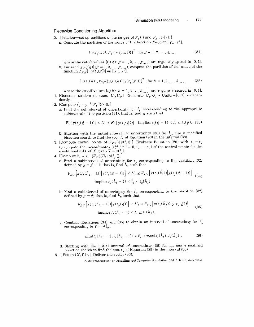
Method of Piecewise Conditioning. The objective of the method of piece-wise conditioning is to accelerate the root-finding operations required to solve
Equations (28) and (29) by exploiting a precomputed partition of the range of
values of the marginal c.d.f. of Y together with the corresponding precom-
puted partitions of the range of values of the conditional c.d.f. of X given Y. Aformal statement of this algorithm is given in the following.
ACM TransactIons on Modeling and Computer Slmulatlon, Vol 5, No 3, July 1995
Simulation Input Modeling . 177
Piecewise Conditioning Algorithm
O. [ Initialize—set up partitions of the ranges of F’Y() and F’x,~( I ~).1
a. Compute the partition of the range of the function Fy(. ) on [ y*, Y*1,
[y(ty(g)), FY{y(tv(g))}lT forg = 132, . . ..g~ax. (31)
where the cutoff values {tv(g ): g = 1,2,. ... g~..} are regularly spaced in [0, 11.
b. For each y(t,(g))(g = 1,2,..., g~., 1 compute the partition of the range of thefunction FxlY[.ly(t,(g))] on [.~.,, X*I,
[x(tz(h)), F’xlY{x(tL(h))l y(tY(g))}lT forh = 1,2,..., h~~k, (32)
where the cutoff values {tX(h): h = 1,2, ..., h~.x} are regularly spaced in [0, 1].1, [Generate random numbers UI, Uz. 1 Generate U], u? - Uniform[O, 11 indepen-
dently.
2. [Compute ;Y = y-l[F~l(ul)]. ]
a. Find the subinterval of uncertainty for fY corresponding to the appropriatesubinterval of the partition (31); that is, find ~ such that
Fy[y(ty(g – l))] < UI s FY[.Y(tY(E))l implies ty(g – 1) < ~, S ty(+?). (33)
b. Starting with the initial interval of uncertainty (33) for ~Y, use a modifiedbisection search to find the root ~y of Equation (28) in the interval (33).
3. [Compute control points of Fxly[.l y(t,)l. 1 Evaluate Equation (26) with t., = f,
to compute the z-coordinates {Z$xly ’: i = O, 1, ..., n ~} of the control points for theconditional c.d.f. of X given Y = y(iY).
4. [Compute ZX= x-l{l’j+.[Uz \y(ZY)l}.
a. Find a subinterval of uncertainty-for iX corresponding to the partition (32)defined by g = ~ – 1; that is, find hl such that
Fxly[x(tJk, - l))ly(t,(g- 1))]< u, s Fxly[x(t.(kl))lY(t,(~ - q (34)
b. Find a subinterval of uncerta@ty for ~X corresponding to the partition (32)defined by g = ~; that is, find h ~ such that
Fxly[x(tJk2 - l))ly(t,(m] < u, = FxlY[x(tx(~2))lY(~y(~))] (35)
implies tz(kz – 1) < i. S tX(Zz).
C. Combine Equations (34) and (35) to obtain an interval of uncertainty for ~Xcorresponding to Y = y(fY):
min{ti(il – l),t~(kz – 1)} < iX S max{tX(kl), tX(kz)}. (36)
d. Starting with the initial interval of uncertainty (36) for iX, use a modifiedbisection search to find the root it of Equation (29) in the interval (36).
5. [ Return (X, Y )T. ] Deliver the vector (30).
ACM Transactions on Modeling and Computer Simulation, Vol. 5, No. 3, July 1995.
178 . M, A Flanigan Wagner and J. R, Wilson
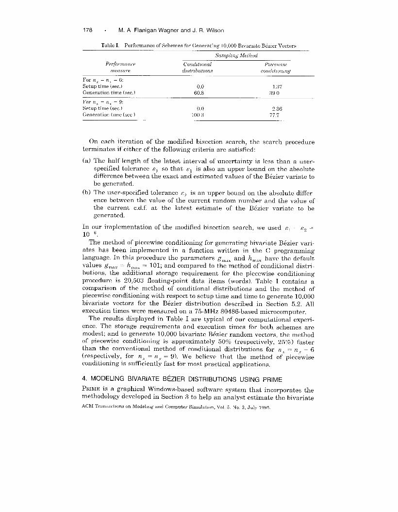
Table I. Performance of Schemes for Generating 10,000 Blvarlate B6zier Vectors
Samphng Method
Performance Condltwnal Pzece wise
measure dlstrlbutlons condltlonlng
For nz = n, = 6:Setup time (sec.) 0.0 1.37Generation time (sec.) 60.8 390
Forrz2 = nv = 9:Setup time (sec.) 0.0 2.36Generation time (see ) 1003 77.7
On each iteration of the modified bisection search, the search procedure
terminates if either of the following criteria are satisfied:
(a)
(b)
The half-length of the latest interval of uncertainty is less than a user-
specified tolerance &l so that ZI is also an upper bound on the absolute
difference between the exact and estimated values of the B6zier variate to
be generated.
The user-specified tolerance Sz is an upper bound on the absolute differ-
ence between the value of the current random number and the value of
the current c.d.f. at the latest estimate of the B6zier variate to be
generated.
In our implementation of the modified bisection search, we used c1 = ez =~~--6
The method of piecewise conditioning for generating bivariate B6zier vari-
ates has been implemented in a function written in the C programming
langaage. In this procedure the parameters g~~X and h~~X have the default
values g~,X = h~,. = 101; and compared to the method of conditional distri-
butions, the additional storage requirement for the piecewise conditioning
procedure is 20,503 floating-point data items (words). Table I contains a
comparison of the method of conditional distributions and the method of
piecewise conditioning with respect to setup time and time to generate 10,000
bivariate vectors for the B6zier distribution described in Section 5.2. All
execution times were measured on a 75-MHz 80486-based microcomputer.
The results displayed in Table I are typical of our computational experi-
ence. The storage requirements and execution times for both schemes are
modest; and to generate 10,000 bivariate B6zier random vectors, the methodof piecewise conditioning is approximately 50% (respectively, 25%) faster
than the conventional method of conditional distributions for n, = n ~ = 6
(respectively, for nX = n-y = 9). We believe that the method of piecewiseconditioning is sufficiently fast for most practical applications.
4. MODELING BIVARIATE BEZIER DISTRIBUTIONS USING PRIME
PRIME is a graphical Windows-based software system that incorporates the
methodology developed in Section 3 to help an analyst estimate the bivariate
ACM TransactIons on Modeling and Computer Simulation, Vol. 5, No. 3, July 1995.
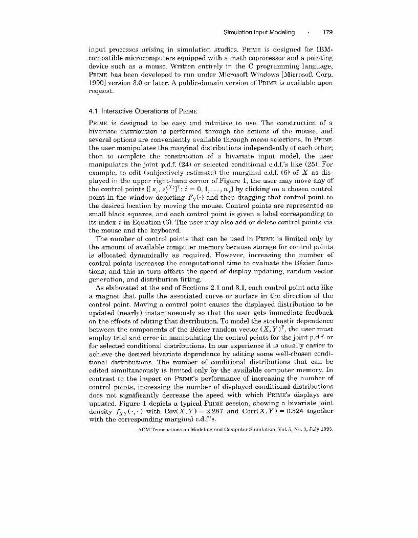
Simulation Input Modeling . 179
input processes arising in simulation studies. PRIME is designed for IBM-
compatible microcomputers equipped with a math coprocessor and a pointing
device such as a mouse. Written entirely in the C programming language,
PRIME has been developed to run under Microsoft Windows [Microsoft Corp.
1990] version 3.0 or later. A public-domain version of PRIME is available upon
request.
4.1 Interactive Operations of PRIME
PRIME is designed to be easy and intuitive to use. The construction of a
bivariate distribution is performed through the actions of the mouse, and
several options are conveniently available through menu selections. In PRIME
the user manipulates the marginal distributions independently of each other;
then to complete the construction of a bivariate input model, the user
manipulates the joint p.d.f. (24) or selected conditional c.d.f.’s like (25). For
example, to edit (subjectively estimate) the marginal c.d.f. (6) of X as dis-
played in the upper right-hand corner of Figure 1, the user may move any of
the control points {[ x,, z~x)]T: i = O, 1,..., n.} by clicking on a chosen control
point in the window depicting Fx(. ) and then dragging that control point to
the desired location by moving the mouse. Control points are represented as
small black squares, and each control point is given a label corresponding to
its index i in Equation (6). The user may also add or delete control points via
the mouse and the keyboard.
The number of control points that can be used in PRIME is limited only by
the amount of available computer memory because storage for control points
is allocated dynamically as required. However, increasing the number of
control points increases the computational time to evaluate the B6zier func-
tions; and this in turn affects the speed of display updating, random vector
generation, and distribution fitting.
As elaborated at the end of Sections 2.1 and 3.1, each control point acts like
a magnet that pulls the associated curve or surface in the direction of the
control point. Moving a control point causes the displayed distribution to be
updated (nearly) instantaneously so that the user gets immediate feedback
on the effects of editing that distribution. To model the stochastic dependence
between the components of the B6zier random vector (X, Y )T, the user must
employ trial and error in manipulating the control points for the joint p.d.f. or
for selected conditional distributions. In our experience it is usually easier to
achieve the desired bivariate dependence by editing some well-chosen condi-
tional distributions. The number of conditional distributions that can be
edited simultaneously is limited only by the available computer memory. In
contrast to the impact on PRIME’S performance of increasing the number of
control points, increasing the number of displayed conditional distributions
does not significantly decrease the speed with which PRIME’S displays are
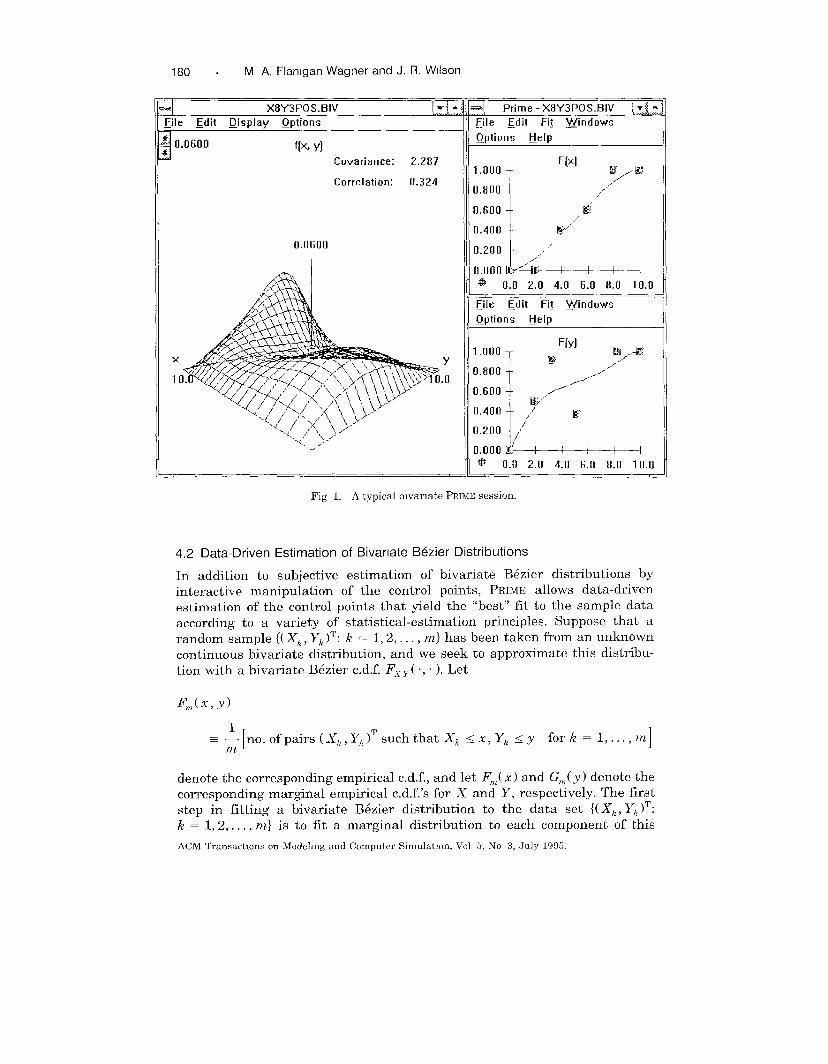
updated. Figure 1 depicts a typical PRIME session, showing a bivariate joint
density &Y(., . ) with COV(X, Y) = 2.287 and Corr(X, Y) = 0.324 together
with the corresponding marginal c.d.f.’s.
ACM Transactions on Modeling and Computer Simulation, Vol. 5, No. 3, July 1995.
180 . M A, Flanlgan Wagner and J. R. Wdson
3 X8Y3P13S.131V F.~ile Edit lJisplay ~ptions
~:0.0600 f[x Y)
Covariance: 2.287
Correlation: 0.324
0.0600
x Y
1 .0
-./
a Prime -X8 Y3POS.BIV
~ile Edit Fi~ windows
Qptions Ijelp
1.000 T0.800 +
,-,../
0,600t
E’,/0.400 + w’
0.2004 /-”1/-~
0.000 k-il~* 0.0 2.0 4.0 6.0 8.0 10.0
~ile Edit Fi~ windows
Qptions Help
1.000
0.800
0.600
0.400[
F(y]W-E
B ./
/“/./’
W“,/
/ K
t0.200 /
0.000 !LL+++++@ o.o 2.0 4.0 6.0 8.0 10.0
Fig 1. A typical bwarlate PRIME session.
4.2 Data-Driven Estimation of Bivarlate B6zier Distributions
In addition to subjective estimation of bivariate B6zier distributions by
interactive manipulation of the control points, PRIME allows data-driven
estimation of the control points that yield the “best” flt to the sample data
according to a variety of statistical-estimation principles. Suppose that a
random sample {( X~, Y~)T: k = 1,2, . . . . m} has been taken from an unknown
continuous bivariate distribution, and we seek to approximate this distribu-
tion with a bivariate B6zier c.d.f. Fx ~-(., “ ). Let
Fn(x, y)
1—— —[no. of pairs (X~, YIZ)T such that X~ < x, Yh < y fork =l,..., m]
m
denote the corresponding empirical c.d.f., and let F~,( x ) and Gn( y ) denote the
corresponding marginal empirical c.d.f.’s for X and Y, respectively. The first
step in fitting a bivariate B6zier distribution to the data set {( Xh, Yk )T:
k=l,2,..., m} is to fit a marginal distribution to each component of this
ACM T,amsactlonson Modellng and Computer Simulation. Vol 5, No 3, JUIY 1995.
Simulation Input Modeling . 181
sample separately. For completeness, we summarize the scheme for data-
driven estimation of univariate B6zier distributions that has been imple-
mented in PRIME as detailed in Wagner and Wilson [ 1~95].
We seek to fit a univariate marginal B6zier c.d.f. Fx[.; nl, x, z(x)] of the
form (6) to the data set {X~: k = 1,..., m}, where
For this purpose we select an appropriate distance function ~{~m(”), flx[.; ~1,
x z(x)]} between the empirical c.d.f. ~n(.) and the fitted c.d.f. ~’[.; nX, x, z(x)].
P;IME uses a nonlinear optimization procedure based on the Nelder-Mead
simplex search algorithm [Nelder and Mead 1964; Olsson and Nelson 1975]
to solve the problem
(minimize d Fn(. ),l$x[.; rz, ,x, z(x)x, Z’x)
1)\
subject to &[x(tX); n,, x, z(x)] > 0 for all tX G [0,1]
(.x) —20 —o ), (37)z(x) = 1
~.
X() < x(l)x ~z > x(m)
1
are the order statistics for the sample { X~ }. The classical fitting methods that
have been incorporated into PRIME include: least squares estimation, mini-
mum LI norm estimation, minimum LX norm estimation, maximum likeli-
hood estimation, moment matching, and percentile matching. Selecting one of
these fitting schemes from a drop-downAmenu implicitly involves selecting an
appropriate distance function d{ F~(. ), I’x[.; nX, x, Z(x ‘]}. The same procedure
is used to fit a univariate marginal B6zier c.d.f. ~Y[.; ny, y, Z(‘)] to the
sample data set {Yh }. Our computational experience indicates that in compar-
ison to other widely used optimization procedures, the Nelder-Mead simplex
search procedure is faster and more stable in solving the optimization prob-
lem (37) for each of the distribution-fitting methods mentioned; see Flanigan
[1993, P. 44] and Swain et al. [19:8].After fitting marginal c.d.f.’s F’x[; rzX, x, z(y)] and fiy[.; nY, y, z(y)] sepa-
rately to the corresponding components of the random sample {( X~, Yk )T:
k = 1,2,..., m}, the user can model the dependencies between these compo-
nents. The dependencies are modeled by moving the control points associated
with either the joint B6zier p.d.f. fxY (”, . ) or selected conditional B&zier
c.d.f.’s or p.d.f.’s until the desired stochastic dependence is achieved. In thenext section we illustrate both subjective and data-driven estimation of
bivariate B6zier distributions using PRIME.
ACM Transactions on Modeling and Computer Simulation, Vol. 5, No 3, July 1995
182 . M, A, Flanlgan Wagner and J, R. Wilson
3 NEGPROC.BIV
~le Edit lJisplay Qptions
db0.900000L fk Y]
Covariance: -0.230
Correlation: -0.369
0.9000
x
F[x]1.000 ~ /0.800
L
/
0.600 ;~(
0.400
/
f $L
0.200{,(.
0.000 ‘ i r-4$ 0.01.22 .43,64.86.0
F[y)1.0001- --0.800
0.600
L
,/’
0.400 f0.200 .J ‘>. >
~o.000_.
@ 0.0 Z.O 4.0 6.0 8.0 10.0
. F~lX=x]
close Edit show
LJpdate !ndep
FfT’lX=2.5]1.000 T 1 >f
!5L-JL0.02.04 .06.08.010.0
F~lY=y]
Qlosc Edit show
Llpdate !ndep
F~lY=7.0]1.000
L
/1, ---0.800 i ‘~0.600
/
Ii
0.400 / !!,
0.200 /,/ “<..20.000 -i
0.01 .22.43.64.86.0
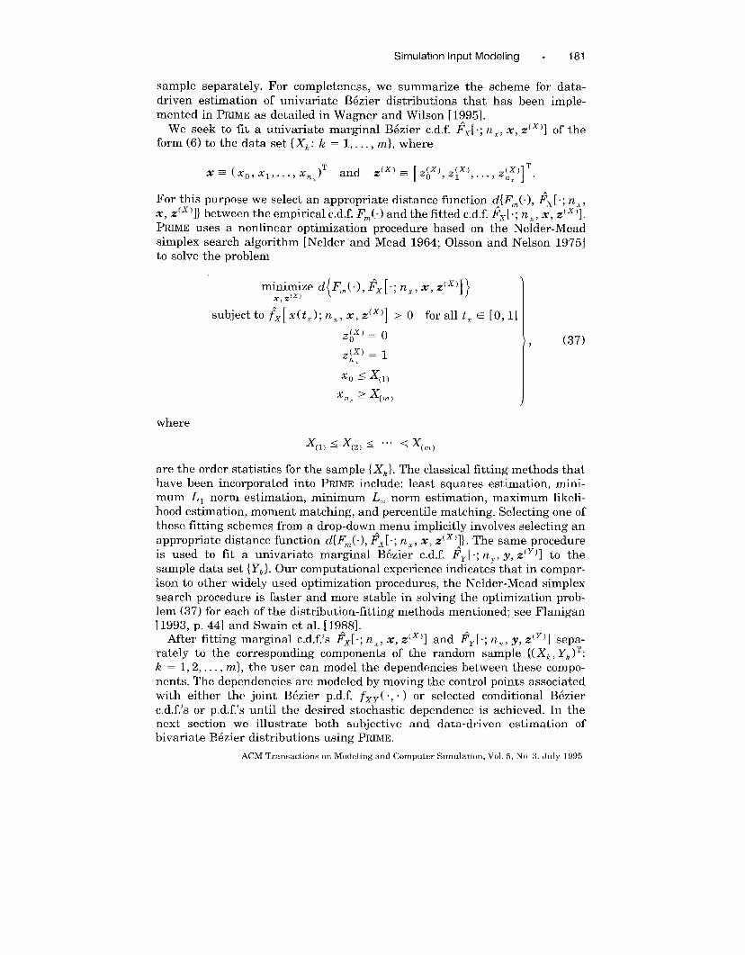
Fig 2. A bivariate distribution of processing times (X, Y)T with Corr(X, Y) = – 0.369
5. EXAMPLES
5.1 Subjectively Fitted Bivariate Bezier Distributions
In the absence of data, PRIME can be used to construct a bivariate input
process conceptualized from subjective information and expertise. For exam-
ple, suppose it is known that the processing times for two successive manu-
facturing operations are negatively correlated, with a correlation coefficient
of —0.37. The processing time is denoted by X, where X is known to have a
minimum value of 2 minutes, a maximum value of 6 minutes, and a most
likely (modal) value of 3 minutes. The second processing time is denoted by
Y, where Y is known to have a minimum value of 3 minutes, a maximumvalue of 9 minutes, and a most likely (modal) value of 6 minutes. To construct
the joint distribution of (X, Y )T, we must first specify the two marginal
distributions. Figure 2 shows the marginal distributions that were built by
moving the control points corresponding to the respective marginal c.d.f.’s
until we matched the lower bounds x,: and y*, the upper bounds x * and y*,
and the modes that were specified. After the marginal c.d.f.’s were fitted, we
manipulated the stochastic dependence between X and Y by moving the
control points associated with the conditional c.d.f.’s FY ,X(.12.5) and Fx ,Y(“17.0)
ACM TransactIons on Modehng and Computer Simulation, Vol 5, No 3, July 1995
.Simulation Input Modeling . 183
> UNDWNEG.131V F~lX=x]
Eile Cdit Display Qptions close Edit show
it 0.1 fk Y]k
Covariance: -5.322
Correlation: -0.645
0.1000
..-,?
x
“\.-
~pdate !ndep
F~lX=9.0]1.000
L
—---....-———0.800 .,,’
0.600 ,,’
0.400 /“
0.200 &;, - -----
0.000
H 0.02.04 .06.08.010.0
~r....LJpdate Indep
F~]Y=2.0]1.000
0.800
i
,’”:
,,,’0.600
1
,’”0.400
0.200 ___.--——
0.000 , t-+--! I
F[x]1.000 ~].800
+
..
1.600.,-
..
F[y]1.000
i
...0.800
0.600
* 0.02.04 .06.08.010.0 @ 0.0 2.0 4.0 6.0 8.0 10.01,
0.02.04.06,08.0100
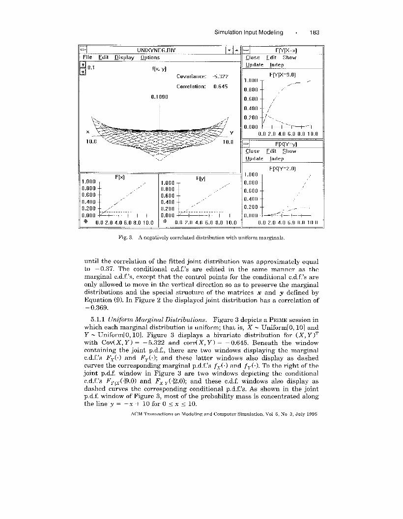
Fig. 3. A negatively correlated distribution with uniform marginals.
until the correlation of the fitted joint distribution was approximately equal
to – 0.37. The conditional c.d.f.’s are edited in. the same manner as the
marginal c.d.f.’s, except that the control points for the conditional c.d,f.’s are
only allowed to move in the vertical direction so as to preserve the marginal
distributions and the special structure of the matrices x and y defined by
Equation (9). In Figure 2 the displayed joint distribution has a correlation of
– 0.369.
5.1.1 Uniform Marginal Distributions. Figure 3 depicts a PRIME session in
which each marginal distribution is uniform; that is, X N Uniform[O, 10] and
Y - Uniform[O, 10]. Figure 3 displays a bivariate distribution for (X, Y )T
with COV(X, Y) = —5.322 and corr(X, Y ) = —0.645. Beneath the window
containing the joint p.d.f., there are two windows displaying the marginal
c.d.f.’s Fx(.) and FY(.); and these latter windows also display as dashed
curves the corresponding marginal p.d.f.’s fx(.) and fy ( .). To the right of the
joint p.d.f. window in Figure 3 are two windows depicting the conditional
c.d.f.’s FY ,X(.19.0) and FXIY(”12.0); and these c.d.f. windows also display as
dashed curves the corresponding conditional p.d.f.’s. As shown in the jointp.d.f. window of Figure 3, most of the probability mass is concentrated along
theline y=–x+lOfor O<x <10.
ACM Transactions on Modeling and Computer Simulation, Vol 5, No 3, July 1995
184 . M, A. Flanlgan Wagner and J. R, Wilson
. X5 Y4POS.BIV
Eile Edit Display LMions
it 0.2k m Y]
Covariance: 2.133
Correlation: 0.539
0.2000
x Y
1 .0
FIx]I .000
F(y]
T
,--- 1.000D.800 If 0.800 T ,(——
Llpdate !ndep
F~lX=3.0]1.000
0.800
L
/0.600
0.400 /
0.200 1/“-– \-
0.000 4 i
0.04.08.0 12.(16.[20.0
R+- F~lY=y]
fJose Cdit show
update !ndep
FpqY=8.o)1.000
0.800
L
/–’-
0.600
0.400
0.200 /’-’~,J:-”. /..-
0.000/
0.02.04 .06.08.010.0
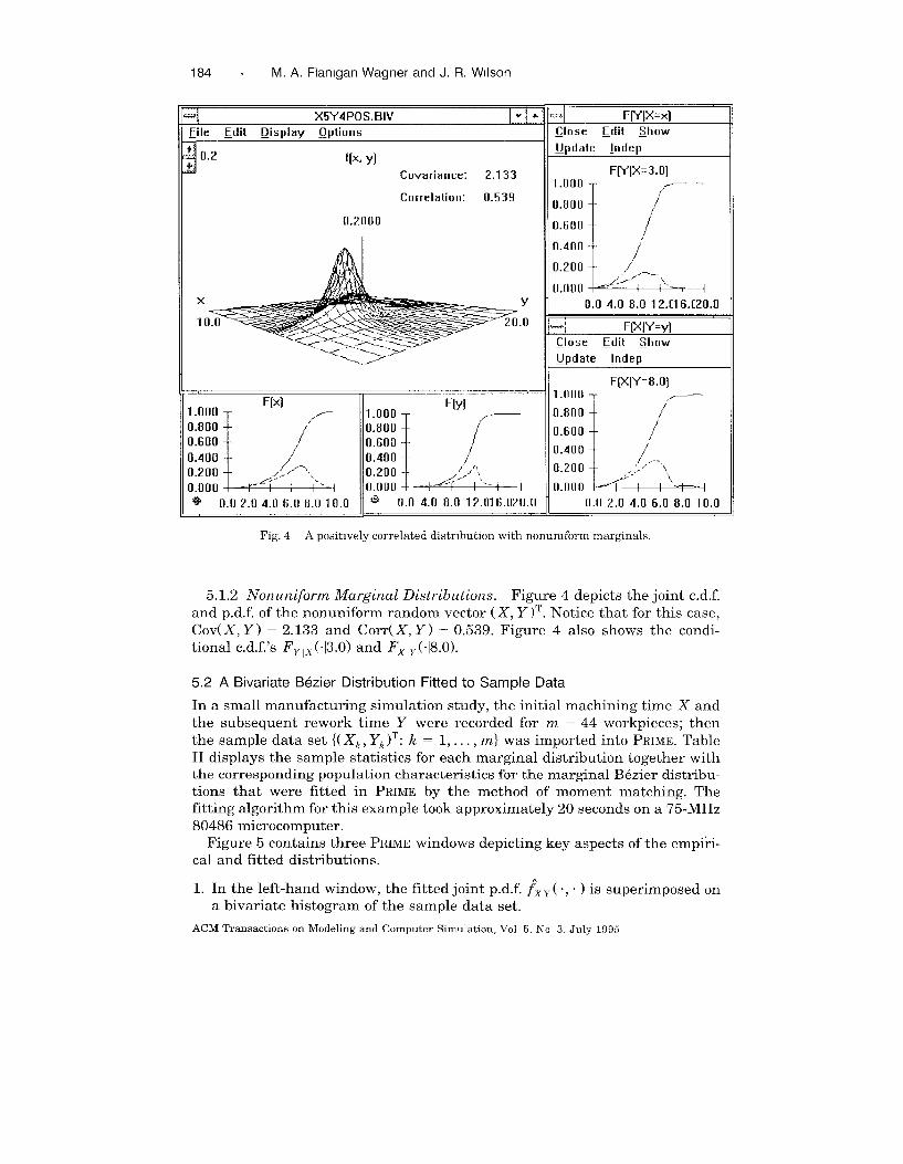
Fig. 4 A positwely correlated distribution with nonumform marginals
5.1.2 Nonuniform Marginal Distributions. Figure 4 depicts the joint c.d.f.
and p.d.f. of the nonuniform random vector (X, Y )T. Notice that for this case,
COV(X, Y) = 2.133 and Corr(X, Y) = 0.539. Figure 4 also shows the condi-
tional c.d.f.’s FY ,x (.13.0) and FXIY(”18.0).
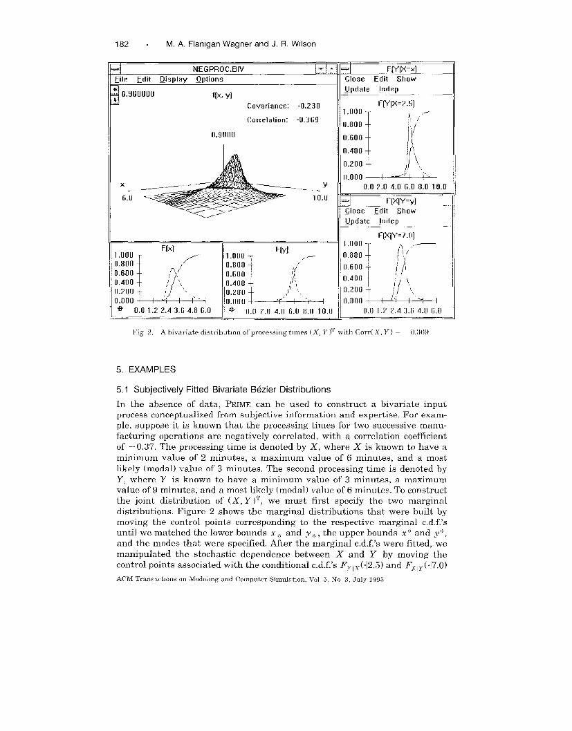
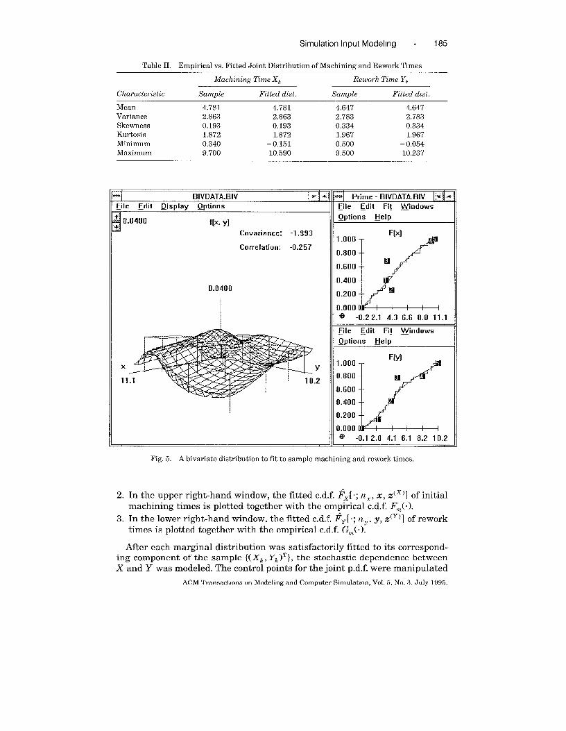
5.2 A Bivariate Bezier Distribution Fitted to Sample Data
In a small manufacturing simulation study, the initial machining time X and
the subsequent rework time Y were recorded for m = 44 workpieces; then
the sample data set {( Xh, Yk )T: k = 1, ..., m} was imported into PRIME. Table
II displays the sample statistics for each marginal distribution together withthe corresponding population characteristics for the marginal B6zier distribu-
tions that were fitted in PRIME by the method of moment matching. The
fitting algorithm for this example took approximately 20 seconds on a 75-MHz
80486 microcomputer.Figure 5 contains three PRIME windows depicting key aspects of the empiri-
cal and fitted distributions.
1. In the left-hand window, the fitted joint p.d.f. &Y (., . ) is superimposed on
a bivariate histogram of the sample data set.
ACM Transactions on Modeling and Computer Simulation, Vol 5, No 3, July 1995
Simulation Input Modeling . 185
Table II. Empirical vs. Fitted Joint Distribution of Machining and Rework Times
Machining Time Xk Rework Time Yk
Characteristic Sample Fitted dist. Sample Fitted dLst,
Mean 4.781 4.781 4.647 4.647Variance 2.863 2.863 2.7’83 2.783Skewness 0.193 0.193 0.334 0.334Kurtosis 1.872 1.872 1.967 1.967Minimum 0.340 –0.151 0.500 –0.054Maximum 9.700 10.590 9.500 10.237
a BIVDATA.BIV &i
~le Edit Qisplay Qptions
4t 0.0400 w Y]kCovariance: -1.993
Correlation: -0.257
0.0400
x Y
11 .2
I
== Prime - BIVDATA. BIV ~~~*
~le Edit Fi! windows
Qptions Help
0.000 kL—tt—A@ .0.22.1 4.3 5.5 8.8 11.1
~le Edit Fi! windows
C)ptions Help
F[y]1.000
1/
.P0.800 mr+f
0.600
0.400 ..
0.000 E.w 1 I ! 1 I@ .0.12,0 4.1 5.1 8.2 10.2
Fig. 5. A bivariate distribution to fit to sample machining and rework times.
2. In the upper right-hand window, the fitted c.d.f. flx[”; rzx, Z, z(x)] of initial
machining times is plotted together with the empirical e.d.f. Fro(.).
3. In the lower right-hand window, the fitted c.d.f. fiy[.; rzy, Y, z(y)] of rework
times is plotted together with the empirical c.d.f. Gin(”).
After each marginal distribution was satisfactorily fitted to its correspond-
ing component of the sample {(XL, Yk )T}, the stochastic dependence between
X and Y was modeled. The control points for the joint p.d.f. ‘were manipulated
ACM TransactIons on Modeling and Computer Simulation, Vol. 5, No. 3, July 1995.

186 . M, A, Flanigan Wagner and J R Wilson
until the theoretical covariance Cov( X, Y) for the fitted distribution matched
the sample covariance G( X, Y ) = – 1.979. For this example, interactively
editing the bivariate B6zier p.d.f. took approximately 30 seconds on a 75-MHz
80486 computer.
6. SUMMARY, CONCLUSIONS, AND RECOMMENDATIONS
6.1 Bivariate Bezier Distribution Families
If ( X, Y )T is a continuous random vector having a bivariate B6zier distribu-
tion function FXY(”, “ ) as defined in Section 3, then the distribution of(X, Y )T has the following properties.
1. The joint c.d.f., represented parametrically by Equation (8) as a B6zier
surface, is similar in form to a B&zier curve. The Bernstein polynomials (2)
are the same basis functions used for both B6zier curves and B6zier
surfaces.
2. The joint p.d.f., fxY(”, “ ), has a closed-form parametric representation as aratio of B6zier functions, as given by Equation (24).
3. The conditional c.d.f.’s, F’xll .(”I . ) and Fyl,y(”l ), have the same parametricform as the univariate marginal c.d.f.’s; and the control points that define
the conditional c.d.f.’s are easily related to the control points that define
the joint c.d.f.
4. The conditional p.d.f.’s, fxlY( 1. ) and fYlx(.l . ‘), have the same parametric
form as the univariate marginal p.d.f.’s; and the control points that define
the conditional p.d.f.’s are easily related to the control points that define
the joint c.d.f.
5. The covariance between X and Y, Cov( X, Y ), has a closed-form expression
given by Equation (27).
6. The parameterization of the bivariate B6zier distribution family is both
natural and open-ended. The coordinates of the control points define the
distribution parameters, and if additional flexibility is required, it is easily
achieved by adding more control points.
6.2 Modeling Simulation Inputs with PRIME
From the user’s point of view, PRIME is an easy-to-use, intuitive, graphical
software system. PRIME provides immediate visual feedback on the user’s
editing of the currently displayed distribution. The user can easily alter an
inappropriately configured distribution by adding, deleting, or relocating one
or more of the relevant control points for the joint p.d.f., the marginal p.d.f.’s
or c.d.f.’s, or selected conditional c.d.f.’s or p.d.f.’s. PRIME also provides a
framework for viewing and manipulating bivariate distributions.
6.3 Recommendations for Future Work
Several aspects of this work require further research and development,
1. Of particular interest is the extension of the methodology to handletrivariate and higher-dimensional distributions. In principle such an ex-
AC!M TransactIons on Modeling and Computer Simulation. Vol 5, No. 3, Ju] y 1995.
Simulation Input Modeling . 187
tension is feasible but cumbersome. Specifically, a trivariate E%zier distri-
bution function FWX Y(”, “ , . ) for the continuous random vector ( W, X, Y)T
with bounded support could be given parametrically by a three-dimen-
sional EKzier surface in four-dimensional Euclidean space, as follows:
R(t,o, tl, ty) = {w(tw),x(tx),y(ty),Fwxy[w(tu,),x(tx),y(ty)]}T
= 5 5 i ~nu,,,(t,,))~nl,t(~x)~ny,,(~.y)~/,,,,j(38)
<’=oi=o]=o
for all tu,, t,, ty = [0, I], where the triply subscripted hypermatrices
1w=[w/,l, J , x=[xr. ,J], ] and Z=[ZY=[Y,,,, j $ /,,,,1 (39),,
each consist of (nU, + 1) x ( nX + 1) X (n ~ + 1) elements respectively defin-
ing the w-, x-, y-, and z-coordinates of the control points
)i= O,l,..., nX; j= 0,1, nY., nY .
To ensure that the c.d.f. F’WYY-( ~, ., “ ) will have the parametric representa-
tion (38) as well as given univariate B6zier marginal c.d.f.’s J’W(” ), Fx(”),
and FY (” ), we must formulate appropriate extensions of Equations (9) and
(10) that apply to the hypermatrices defined in Equation (39). Moreover, itis desirable to ensure that the bivariate marginals F’wx(., . ), F’Wy (”, . ),
and FXy ( ., . ) should have the same functional form (8) as the bivariate
I%zier c.d.f.’s developed in this article. We have verified that the desired
extension of Equations (9) and (10) to trivariate and higher-dimensional
B6zier distributions is theoretically feasible, but the resulting trivariate
distribution is awkward to use.
Because the desired parametric form (38) for the trivariate B6zier c.d.f.
can be arranged in principle, the analyses of the associated joint p.d.f., of
the conditional B&zier distributions, and of the covariance between any
two B6zier variates will parallel closely the developments presented in
Sections 3.4, 3.5, and 3.6, respectively. Although the sampling scheme of
Section 3.7 can be adapted to the generation of trivariate B6zier vectors, it
is unclear whether such a sampling scheme is generally practical for
higher-dimensional I%izier vectors.
2. For subjective estimation of continuous biva riate distributions, we also
require more comprehensive techniques for visually representing and
manipulating general types of stochastic dependence.
3. For data-driven estimation of continuous bivariate distributions, we re-
quire fully automated fitting schemes to estimate not only the marginal
distributions of the target random vector but also the stochastic depen-
dence between the two components of that random vector.
All these topics are the subject of ongoing work.
ACM TransactIons on Modeling and Computer Simulation, Vol. 5, NO 3, July 1995
188 . M, A. Flanlgan Wagner and J. R Wilson
ACKNOWLEDGMENTS
The authors thank Stephen D. Roberts, Bruce Schmeiser, and Arnold Sweet
for many enlightening discussions on this paper. The authors also thank Paul
Fishwick and Robert O’Keefe, the Special Issue Coeditors, and the three
anonymous referees for several suggestions that improved the readability of
this paper.
REFERENCES
CARIO, M. C. AND NELSON, B. L. 1995. Autoregressive to anything: Time series input processes
for simulation. Working Paper, Dept of Industrial, Welding and Systems Engineering, Ohio
State Univ., Columbus.
CONTII, S. D. AND DE BOOR, C. 1980. Elementary Numerical Analysls: An Algorithmic Ap-
proach, 3rd cd., McGraw-Hill, New York.DEBROTA,D J,, DITTUS,R S., ROBERTS,S. D., ANDWILSON,J. R. 1989. Visual interactive
fitting of bounded Johnson distributions, Simulation 52, 5 (May), 199-205.FARIN, G. 1990, CurLes and Surfaces for Computer Aided GeometrLc Design; A Practical
GuLde, 2nd cd., Academic Press, New York.
FLANICAN, M. A. 1993, A flexible, interactive, graphical approach to modehng stochastic inputprocesses. Ph D, dissertation, School of Industrial Engineering, Purdue Univ., West Lafayette,Ind.
JAGERMAN, D. L, AND MELAMED, B. 1992a. The transition and autocorrelation structure of TESprocesses, Part I: General theory. Comm un. Stat. Stoch, Models 8, 2, 193–2 19.
JAGF,RMAN,D. L. mm MELAMED, B. 1992b, The transition and autocorrelation structure of TES
processes, Part II: Special cases. Commun. Stat. Stoch. Models 8, 3, 499–527.
JOHNSON, N. L. 1949a. Systems of frequency curves generated by methods of translation.Btometrika 36, 149-176.
JOHNSON,N. L. 1949b. Bivariate distributions based on simple translation systems. Bzometrtka
36, 297-304,
JOI*NSON, M, E. 1987. Multiuarlate Statistical Simulation. Wiley, New York.
LEWIS, P, A. W AND ORAV, E. J. 1989. S{mulatzon Methodology for Statisticians, Operations
Anal-vsts, and Engzneers, Vol. 1. Wadsworth & Brooks/Cole Advanced Books & Software,Pacific Grove, Cahf.
MELAMED, B., Hn.L, J. R , AND GOLDSMAN, D. 1992. The TES methodology: Modeling empirical
stationary time series, In proceedings of the 1992 Winter Simulation Conference, Institute ofElectrical and Electronics Engineers. Piscataway, N.J., 135-144.
MICROSOFT CORIWRATION. 1990. User’s Manual for the Windows Software Development KLt,
Microsoft Corporation, Redmond, Wash.
NELDER, J. A. AND MEAI), R. 1964. A simplex method for function minimization, Comput, J, 7,
308-313.
OLSSON, D, M. AND NELSON, L. S. 1975. The Nelder-Mead simplex procedure for functionminimization. Technonzetrics 17, 1,45–51.
PRITSRER,A. A. B., MARTIN, D. L., REUST, J. S., WAGNER, M. A,, WILSON, J R., KUHL, M. E., DAILY,O. P., HARPER, A. M., EDWARDS, E. B., B~NNETT, L. E., ALLEN, M. D., ROBERTS, J. P,, ANDBURDJCIi, J. F. 1995. Organ transplantation policy evaluation. In Proceedings of the 1995
Winter Stmulatzon Conference. Institute of Electrical and Electronics Engineers, Plscataway,N.J. (to appear).
STANFIELD, P. M. AND WILSON, J. R, 1993. Multivariate input modeling with Johnson distribu-tions, Tech. Rep. 93-11, Dept. of Industrial Engineering, North Carolina State Univ., Raleigh.
SWAIN, J. J., VENRATRAMAN, S., AND WILSON, J. R. 1988. Least-squares estimation of distribu-tion functions in Johnson’s translation system. J. Stat. Comput. Slmul. 29, 271–297.
WAGNER, M. A. F. AND WILSON, J. R. 1995 Using univariate B6zier distributions to modelsimulation input processes. IZE Transactions (to appear).
ACM Transactions on Modeling and Computer Slmulatlon, Vol 5, No 3, July 1995,

Simulation Input Modellng . 189
WAGNER, M. A. F. AND WILSON, J. R. 1994. Using bivariate B6zier distributions to modelsimulation input processes. In Proceedings of the 1994 Winter Simulation Conference (Orlando,FL, Dec. 11-14), Institute of Electrical and Electronics Engineers, Piscataway, N.J., 324-331.
WAGNER,M. A. F. ANDWILSON,J. R. 1993. Using univariate B6zier distributions to modelsimulation input processes.In Proceedings of the 1993 Winter Simulation Conference. Institute
of Electrical and Electronics Engineers, Piscataway, N.J., 365–373.
Received August 1994; revised August 1995; accepted August 1995
ACM TransactIons on Modeling and Computer Simulation, Vol. 5, No. 3, July 1995.