Embed Size (px)
Citation preview

Graph Theory for Network
Science
Dr. Natarajan Meghanathan
Associate Professor
Department of Computer Science
Jackson State University, Jackson, MS
E-mail: [email protected]

Networks or Graphs• We typically use the terms interchangeably.• Networks – refers to real systems
– WWW: network of web pages connected by URLs
– Society: network of individuals connected by family, friendship or professional ties
– Metabolic network: sum of all chemical reactions that take place in a cell
• Graphs: Mathematical representation of the networks– Web graph, Social graph, Metabolic graph
Real systems of quite different nature can
have the same network representation• Even though these real systems have different nature, appearance or scope,
they can be represented as the same network (graph)
• Internet – connected using routers
• Actor network – network of actors who acted together in at least one movie
• Protein-Protein Interaction (PPI) network – two proteins are connected if there is experimental evidence that they can bind each other in the cell
Internet
Actor Network
PPI
Network
Graph
Fig. 2.3: Barabasi
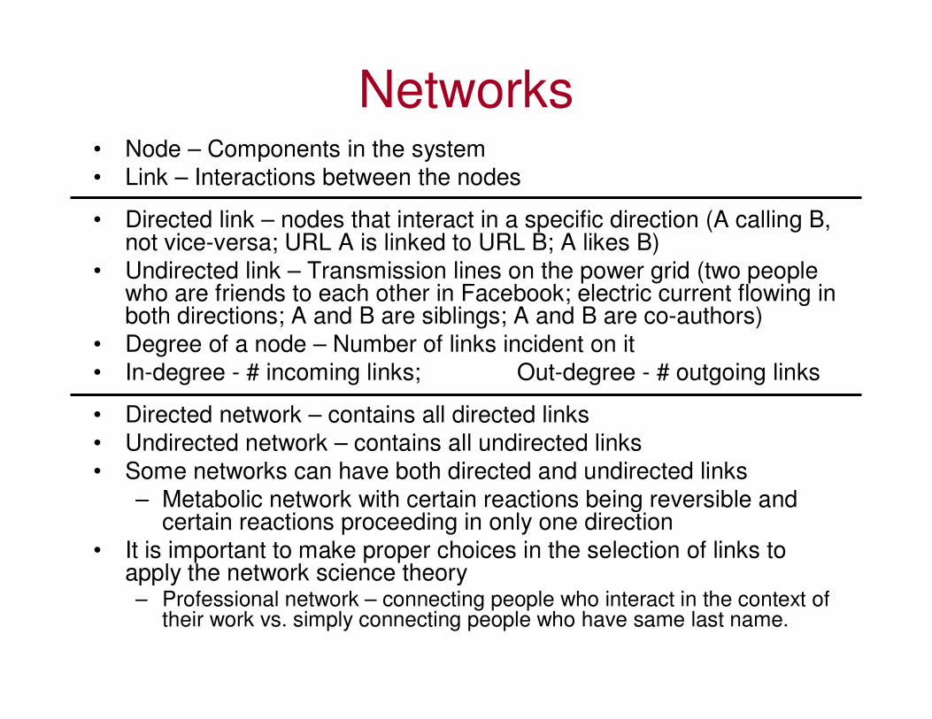
Networks• Node – Components in the system
• Link – Interactions between the nodes
• Directed link – nodes that interact in a specific direction (A calling B, not vice-versa; URL A is linked to URL B; A likes B)
• Undirected link – Transmission lines on the power grid (two people who are friends to each other in Facebook; electric current flowing in both directions; A and B are siblings; A and B are co-authors)
• Degree of a node – Number of links incident on it
• In-degree - # incoming links; Out-degree - # outgoing links
• Directed network – contains all directed links
• Undirected network – contains all undirected links
• Some networks can have both directed and undirected links
– Metabolic network with certain reactions being reversible and certain reactions proceeding in only one direction
• It is important to make proper choices in the selection of links to apply the network science theory– Professional network – connecting people who interact in the context of
their work vs. simply connecting people who have same last name.

Edge Attributes• Weight (e.g., frequency of communication)
• Ranking (choice of dining parameters)
• Type (friend, relative, co-worker)
Source: girls school dormitory dining-table
partners, 1st and 2nd choices (Moreno,
The sociometry reader, 1960)
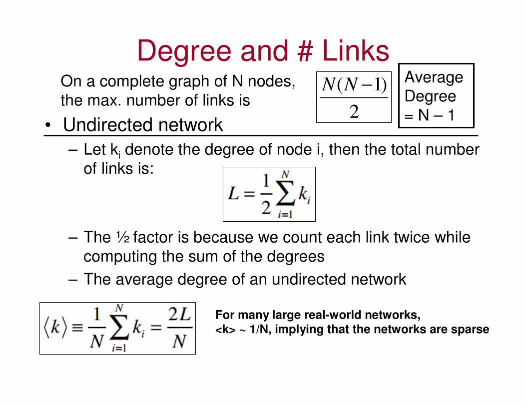
Degree and # Links
• Undirected network
– Let ki denote the degree of node i, then the total number
of links is:
– The ½ factor is because we count each link twice while
computing the sum of the degrees
– The average degree of an undirected network
On a complete graph of N nodes,
the max. number of links is 2
)1( −NN Average Degree
= N – 1
For many large real-world networks,
<k> ~ 1/N, implying that the networks are sparse

Degree and # Links• Directed Network
– Let kiin and ki
out denote the incoming and outgoing degrees of node i.
– The total number of links:
– Average degree of a directed network is:
–
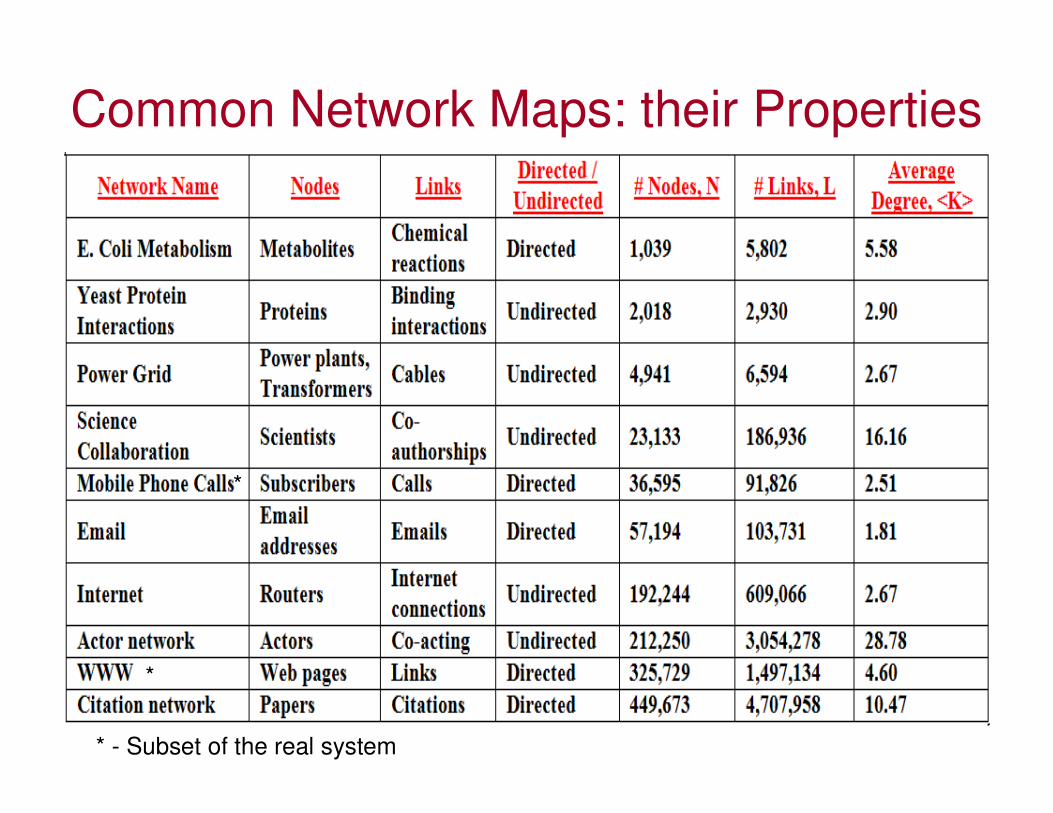
Common Network Maps: their Properties
*
*
* - Subset of the real system
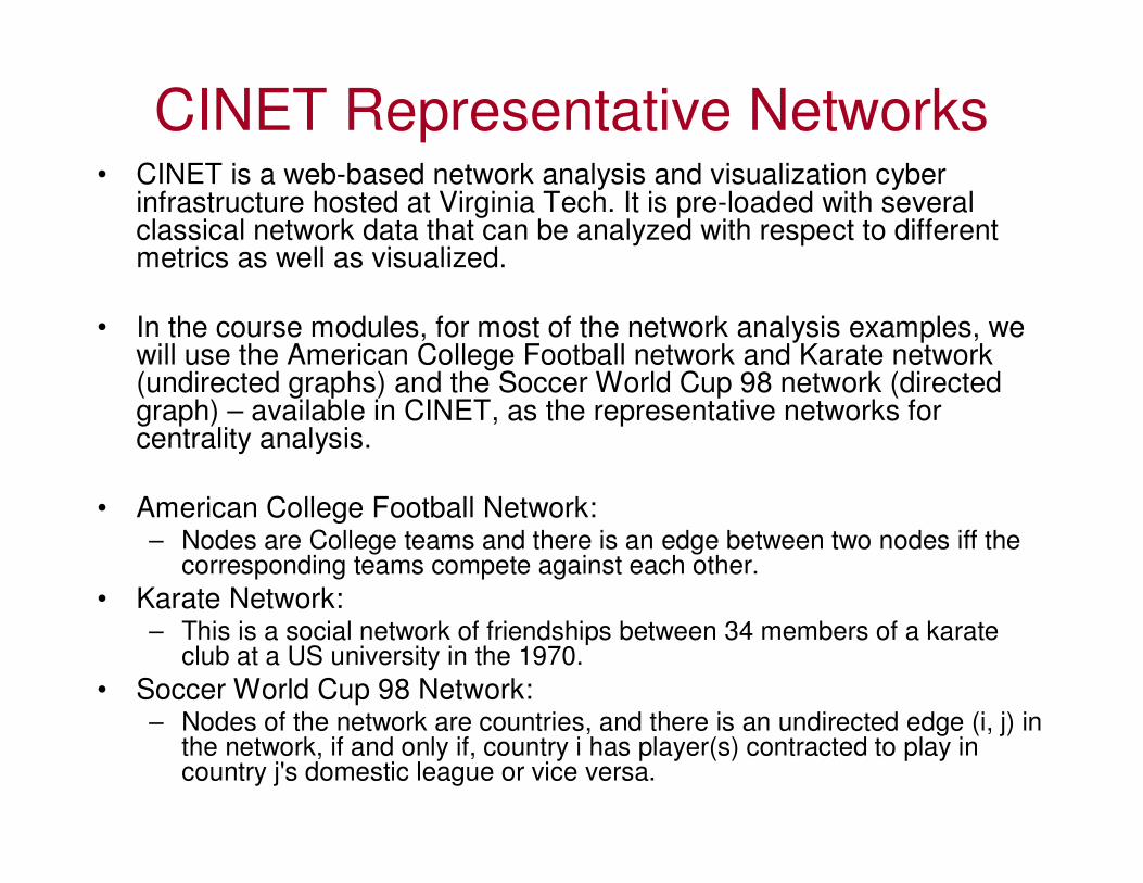
CINET Representative Networks• CINET is a web-based network analysis and visualization cyber
infrastructure hosted at Virginia Tech. It is pre-loaded with several classical network data that can be analyzed with respect to different metrics as well as visualized.
• In the course modules, for most of the network analysis examples, we will use the American College Football network and Karate network (undirected graphs) and the Soccer World Cup 98 network (directed graph) – available in CINET, as the representative networks for centrality analysis.
• American College Football Network: – Nodes are College teams and there is an edge between two nodes iff the
corresponding teams compete against each other.
• Karate Network:– This is a social network of friendships between 34 members of a karate
club at a US university in the 1970.
• Soccer World Cup 98 Network: – Nodes of the network are countries, and there is an undirected edge (i, j) in
the network, if and only if, country i has player(s) contracted to play in country j's domestic league or vice versa.
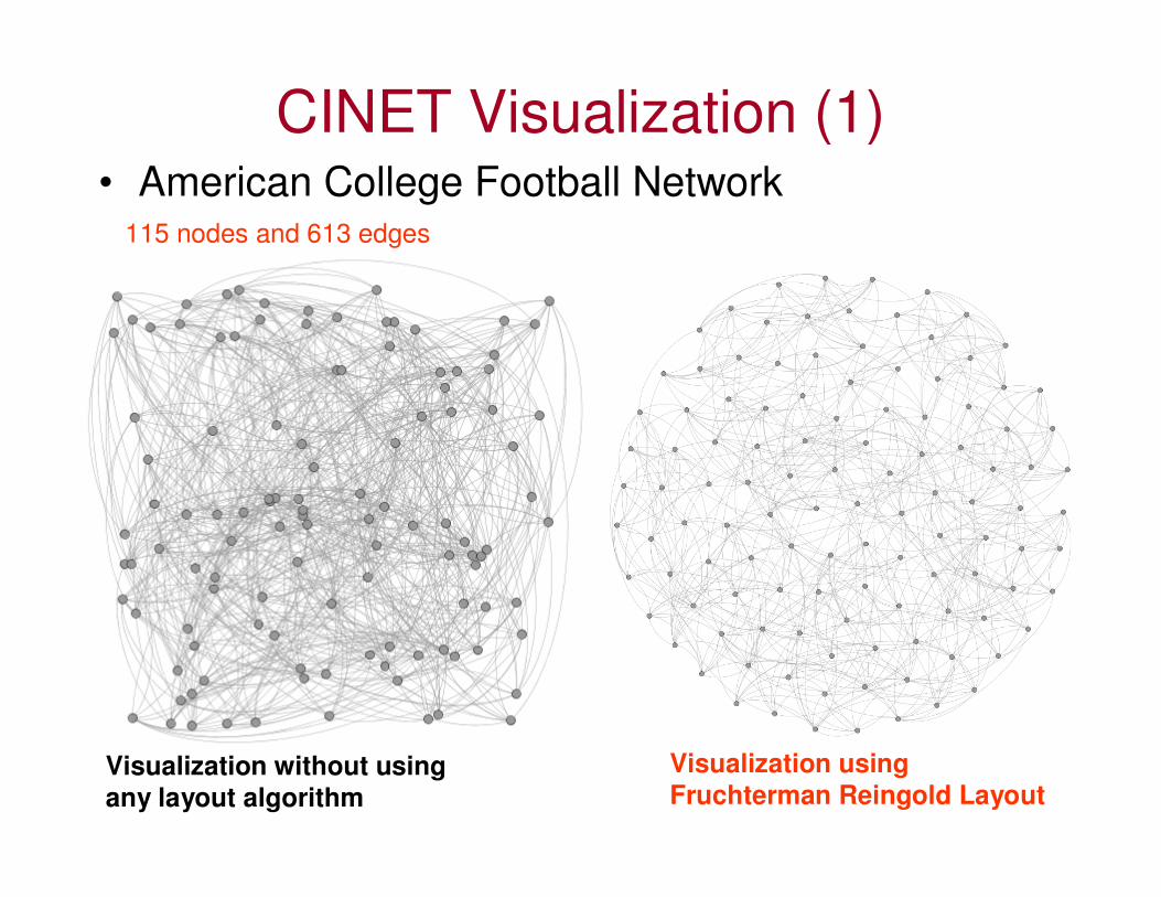
CINET Visualization (1)• American College Football Network
115 nodes and 613 edges
Visualization without using any layout algorithm
Visualization using Fruchterman Reingold Layout
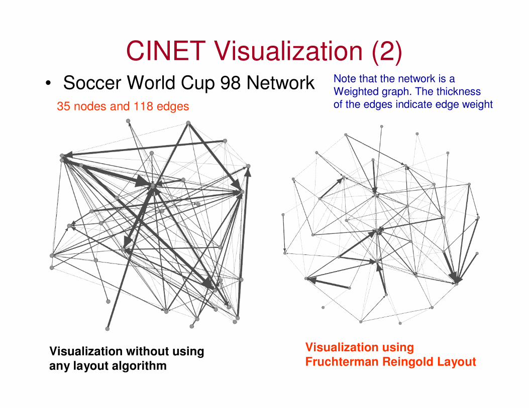
CINET Visualization (2)• Soccer World Cup 98 Network
35 nodes and 118 edges
Visualization without using any layout algorithm
Visualization using Fruchterman Reingold Layout
Note that the network is aWeighted graph. The thicknessof the edges indicate edge weight
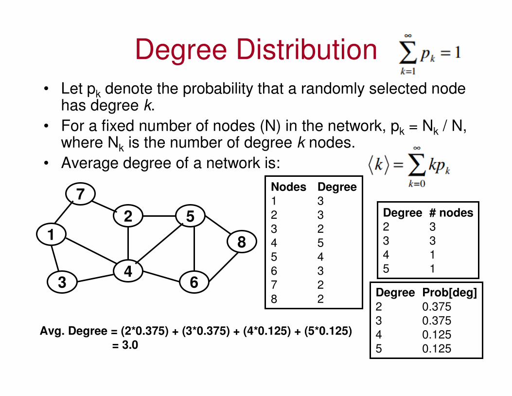
Degree Distribution
• Let pk denote the probability that a randomly selected node has degree k.
• For a fixed number of nodes (N) in the network, pk = Nk / N, where Nk is the number of degree k nodes.
• Average degree of a network is:
12
34
5
6
7
8
Nodes Degree
1 3
2 3
3 2
4 5
5 4
6 3
7 2
8 2
Degree # nodes
2 3
3 3
4 1
5 1
Degree Prob[deg]
2 0.375
3 0.375
4 0.125
5 0.125
Avg. Degree = (2*0.375) + (3*0.375) + (4*0.125) + (5*0.125)= 3.0
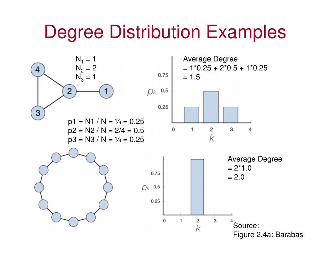
Degree Distribution Examples
N1 = 1
N2 = 2
N3 = 1
p1 = N1 / N = ¼ = 0.25
p2 = N2 / N = 2/4 = 0.5
p3 = N3 / N = ¼ = 0.25
Average Degree
= 1*0.25 + 2*0.5 + 1*0.25
= 1.5
Average Degree
= 2*1.0
= 2.0
Source:
Figure 2.4a: Barabasi

k
p(k) p(k)
k
k
p(k) p(k)
!)(
k
kekp
kk−
=
Poisson
Distribution
( )
−−
=2
2
2
2
1)(
k
kk
k
ekpσ
πσ
Gaussian
Distribution
kkekp
/~)(
−
Exponential
Distribution
γ−kkp ~)(
Power-Law
Distribution
k
(e.g., Star Graphs)
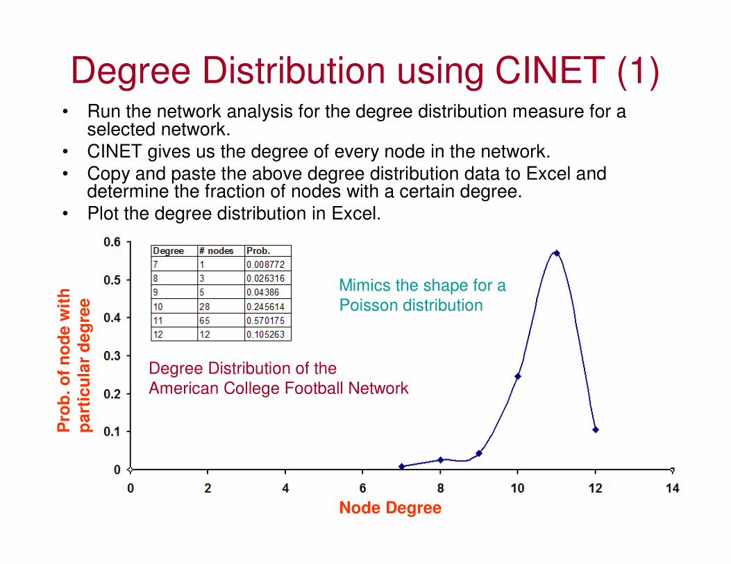
Degree Distribution using CINET (1)• Run the network analysis for the degree distribution measure for a
selected network.
• CINET gives us the degree of every node in the network.
• Copy and paste the above degree distribution data to Excel and determine the fraction of nodes with a certain degree.
• Plot the degree distribution in Excel.
Node Degree
Pro
b.
of
no
de
wit
h
pa
rtic
ula
r d
eg
ree
Mimics the shape for a
Poisson distribution
Degree Distribution of the
American College Football Network
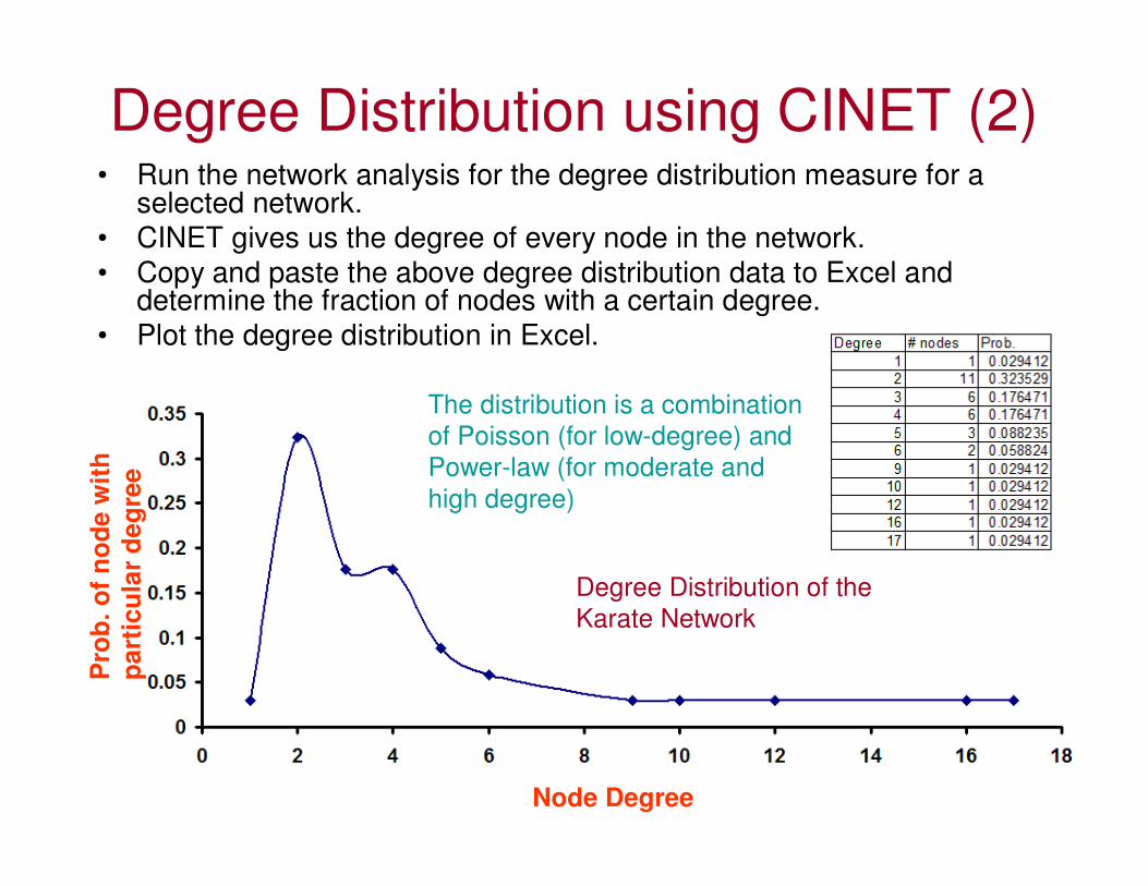
Degree Distribution using CINET (2)• Run the network analysis for the degree distribution measure for a
selected network.
• CINET gives us the degree of every node in the network.
• Copy and paste the above degree distribution data to Excel and determine the fraction of nodes with a certain degree.
• Plot the degree distribution in Excel.
Node Degree
Pro
b.
of
no
de
wit
h
pa
rtic
ula
r d
eg
ree
The distribution is a combination
of Poisson (for low-degree) and
Power-law (for moderate and
high degree)
Degree Distribution of the
Karate Network
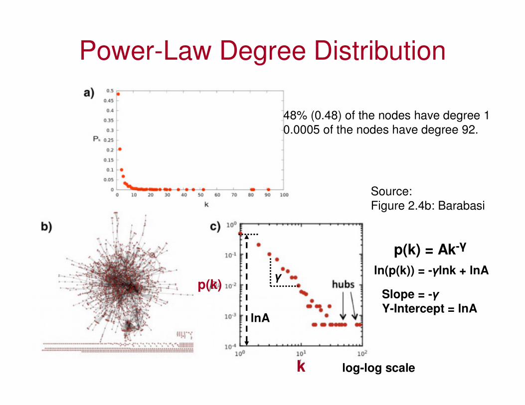
Power-Law Degree Distribution
48% (0.48) of the nodes have degree 1
0.0005 of the nodes have degree 92.
log-log scale
Source:
Figure 2.4b: Barabasi
ln(p(k)) = -γlnk + lnA
Slope = -γ
Y-Intercept = lnAlnA
γ
p(k) = Ak-γ
k
p(k)
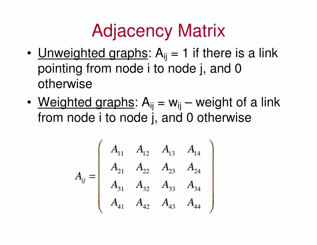
Adjacency Matrix• Unweighted graphs: Aij = 1 if there is a link
pointing from node i to node j, and 0
otherwise
• Weighted graphs: Aij = wij – weight of a link
from node i to node j, and 0 otherwise
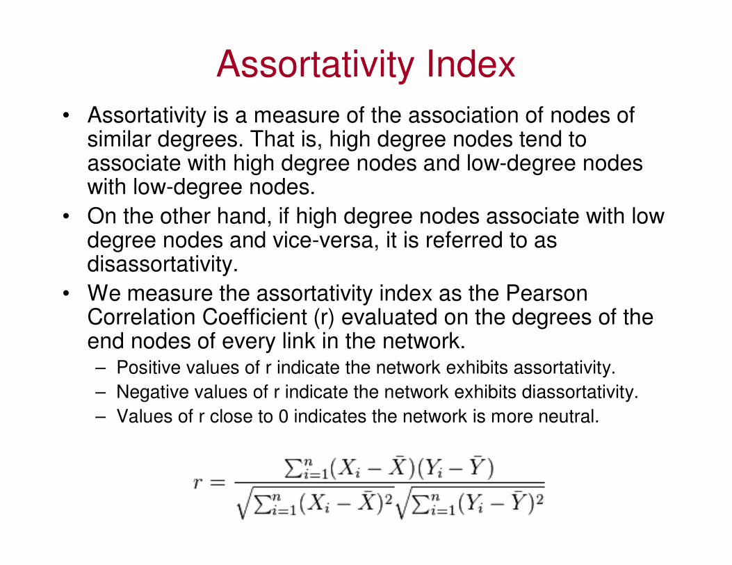
Assortativity Index
• Assortativity is a measure of the association of nodes of similar degrees. That is, high degree nodes tend to associate with high degree nodes and low-degree nodes with low-degree nodes.
• On the other hand, if high degree nodes associate with low degree nodes and vice-versa, it is referred to as disassortativity.
• We measure the assortativity index as the Pearson Correlation Coefficient (r) evaluated on the degrees of the end nodes of every link in the network.– Positive values of r indicate the network exhibits assortativity.
– Negative values of r indicate the network exhibits diassortativity.
– Values of r close to 0 indicates the network is more neutral.
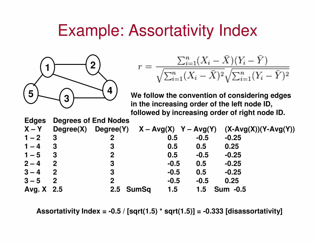
Example: Assortativity Index
1 2
345
Edges Degrees of End Nodes
X – Y Degree(X) Degree(Y) X – Avg(X) Y – Avg(Y) (X-Avg(X))(Y-Avg(Y))
1 – 2 3 2 0.5 -0.5 -0.25
1 – 4 3 3 0.5 0.5 0.25
1 – 5 3 2 0.5 -0.5 -0.25
2 – 4 2 3 -0.5 0.5 -0.25
3 – 4 2 3 -0.5 0.5 -0.25
3 – 5 2 2 -0.5 -0.5 0.25
Avg. X 2.5 2.5 SumSq 1.5 1.5 Sum -0.5
Assortativity Index = -0.5 / [sqrt(1.5) * sqrt(1.5)] = -0.333 [disassortativity]
We follow the convention of considering edges
in the increasing order of the left node ID,
followed by increasing order of right node ID.

Assortativity of Social Networks
Network # Nodes Assortativity IndexPhysicsCo-authorship 52,909 0.363Film actor
Collaborations 449,913 0.208Company Directors 7,673 0.276E-mail AddressBooks 16,881 0.092In real world, most of the social networks are assortative and the non-social
Networks are typically disassortative. However, there are some exceptions.
Network Assortativity Index Network Assortativity Index
Drug Users -0.118 Roget’s Thesaurus 0.174
Karate Club -0.476 Protein Structure 0.412
Students dating -0.119 St Marks Food Web 0.118
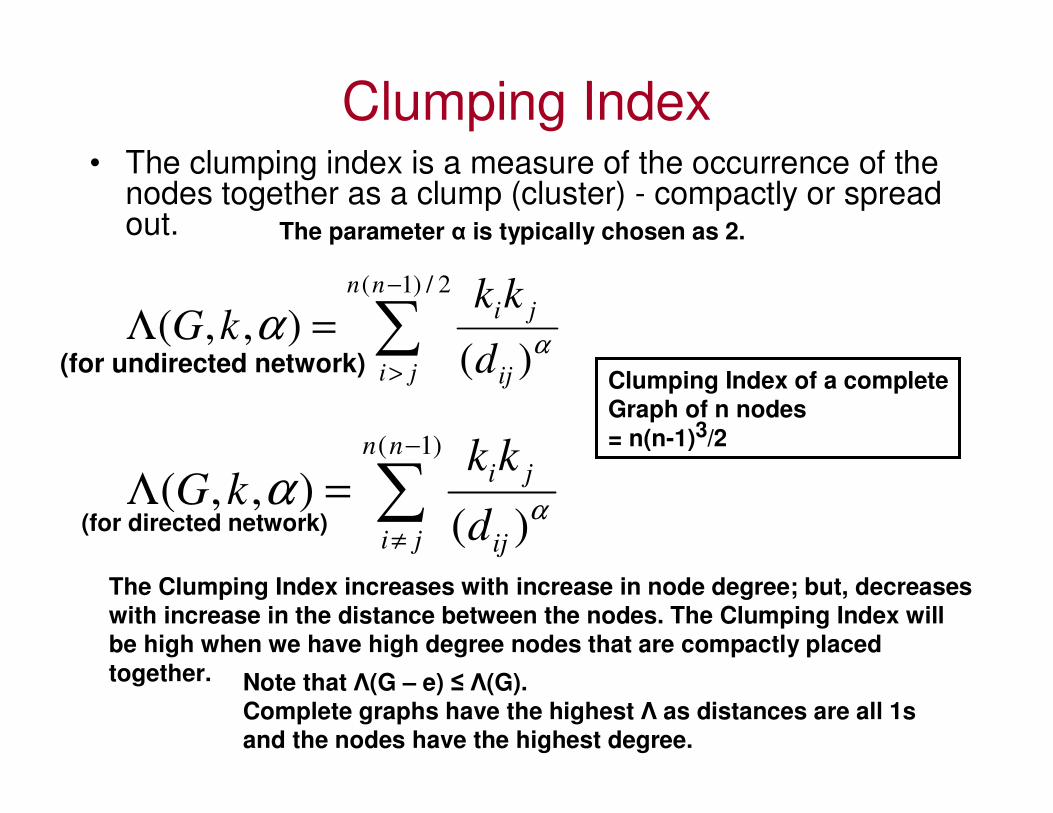
Clumping Index• The clumping index is a measure of the occurrence of the
nodes together as a clump (cluster) - compactly or spread out.
∑−
>
=Λ2/)1(
)(),,(
nn
ji ij
ji
d
kkkG
αα
(for undirected network)
∑−
≠
=Λ)1(
)(),,(
nn
ji ij
ji
d
kkkG
αα
(for directed network)
The Clumping Index increases with increase in node degree; but, decreases
with increase in the distance between the nodes. The Clumping Index will
be high when we have high degree nodes that are compactly placed
together.
The parameter α is typically chosen as 2.
Note that Λ(G – e) ≤ Λ(G). Complete graphs have the highest Λ as distances are all 1s
and the nodes have the highest degree.
Clumping Index of a complete
Graph of n nodes
= n(n-1)3/2

Clumping Index has nothing to do with assortativity or disassortativity.
Assortativity Index = 0.118
High ClumpingAssortativity Index = 0.129
Low Clumping
Assortativity Index = -0.304
High ClumpingAssortativity Index = -0.227
Low Clumping

Clumping Index Examples 1 and 2
1 2
345
Node Degree Distance (a)
Pair Product dij dij2 ---
(a) (b) (b)
1 – 2 6 1 1 6
1 – 3 6 2 4 1.5
1 – 4 9 1 1 9
1 – 5 6 1 1 6
2 – 3 4 2 4 1
2 – 4 6 1 1 6
2 – 5 4 2 4 13 – 4 6 1 1 63 – 5 4 1 1 4
4 – 5 6 2 4 1.5
3 2
2
2
3
Λ = 42
1 2 3 44 5
1 2 2 2 1
Node Degree Distance (a)
Pair Product dij dij2 ---
(a) (b) (b)
1 – 2 2 1 1 2
1 – 3 2 2 4 0.5
1 – 4 2 3 9 0.22
1 – 5 1 4 16 0.063
2 – 3 4 1 1 4
2 – 4 4 2 4 1
2 – 5 2 3 9 0.22
3 – 4 4 1 1 4
3 – 5 2 2 4 0.54 – 5 2 1 1 2
Λ = 14.5

Clumping Index
Example 3
1 2
34 5
Node Out In Degree Distance (a)
Pair deg deg Product dij dij2 ---
(a) (b) (b)
1->2 2 2 4 1 1 4
1->3 2 3 6 1 1 6
1->4 2 0 0 ∞ ∞ N/A
1->5 2 1 2 2 4 0.5
2->1 1 1 1 ∞ ∞ 0
2->3 1 3 3 1 1 3
2->4 1 0 0 ∞ ∞ N/A
2->5 1 1 1 2 4 0.5
3->1 1 1 1 ∞ ∞ 0
3->2 1 2 2 2 4 0.5
3->4 1 0 0 ∞ ∞ N/A
3->5 1 1 1 1 1 1.0
4->1 2 1 2 1 1 2.0
4->2 2 2 4 3 9 0.44
4->3 2 3 6 1 1 6.0
4->5 2 1 2 2 4 0.5
5->1 1 1 1 ∞ ∞ 0.0
5->2 1 2 2 1 1 2.05->3 1 3 3 2 4 0.75
5->4 1 0 0 ∞ ∞ N/A
(2,1) (1,2)
(2,0) (1,3) (1,1)
(out deg, in deg)
Clumping Index = 27.19
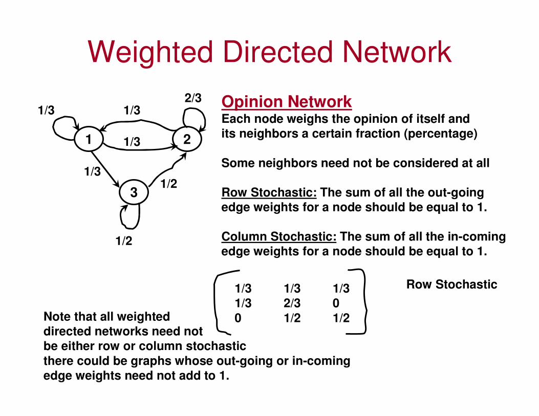
Weighted Directed Network
1 2
3
1/32/3
1/2
1/2
1/3
1/3
1/3
Opinion NetworkEach node weighs the opinion of itself and
its neighbors a certain fraction (percentage)
Some neighbors need not be considered at all
Row Stochastic: The sum of all the out-going
edge weights for a node should be equal to 1.
Column Stochastic: The sum of all the in-coming
edge weights for a node should be equal to 1.
1/3 1/3 1/3
1/3 2/3 0
0 1/2 1/2
Row Stochastic
Note that all weighted
directed networks need not
be either row or column stochastic
there could be graphs whose out-going or in-coming
edge weights need not add to 1.
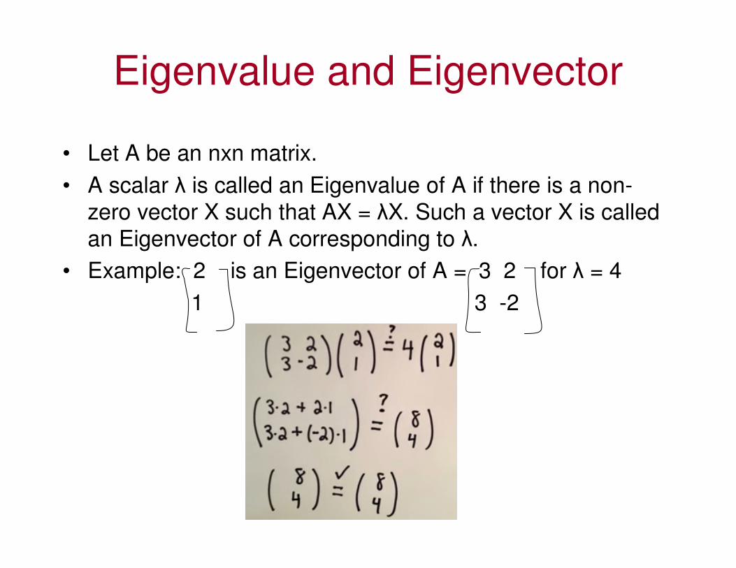
Eigenvalue and Eigenvector
• Let A be an nxn matrix.
• A scalar λ is called an Eigenvalue of A if there is a non-
zero vector X such that AX = λX. Such a vector X is called
an Eigenvector of A corresponding to λ.
• Example: 2 is an Eigenvector of A = 3 2 for λ = 4
1 3 -2

Finding Eigenvalues and Eigenvectors(4) Solving for λ:
(λ – 8) (λ + 2) = 0
λ = 8 and λ = -2 are the Eigen values
(5) Consider A – λ I
Let λ = 8
= B
Solve B X = 0
-1 3
3 -9
X1
X2= 0
0
-X1 + 3X2 = 0
3X1 – 9X2 = 0
X1 = 3X23X1 = 9X2 � X1 = 3X2
If X2 = 1;
X1 = 3
3
1is an eigenvector
for λ = 8

Finding Eigenvalues and Eigenvectors
For λ = -2
7- (-2) 3
3 -1 – (-2)
=9 3
3 1
Solve B X = 0
9 3
3 1
X1
X2= 0
0
9X1 + 3X2 = 0
3X1 + X2 = 0
X2 = - 3X1
If X1 = 1;
X2 = -3
1
-3is an eigenvector
for λ = -2
X2 = - 3X1
Verification
AX = λX
For λ = 8 and X = 3
1
A = 7 3
3 -1
7 3
3 -1
3
1= 24
8= 8
3
1

Spectral Radius (Network Index)• The index of the network or the spectral radius of the node
adjacency matrix A is the largest Eigenvalue of A, denoted λ1(A).
• The largest Eigen value of a connected undirected network is a unique positive value whose corresponding Eigenvector is the principal Eigenvector of the network.
• If kmin, kavg, kmax are the minimum, average and maximum node degrees, then:
kmin ≤ kavg ≤ λ1(A) ≤ kmax
Use this website to determine Eigenvalues and Eigenvectors for a matrix. http://www.arndt-bruenner.de/mathe/scripts/engl_eigenwert.htm
The largest Eigenvalue is 2.4811. 1 2
345
kmin = 2; kmax = 3; kavg = 2.42 < 2.4 < 2.4811 < 3
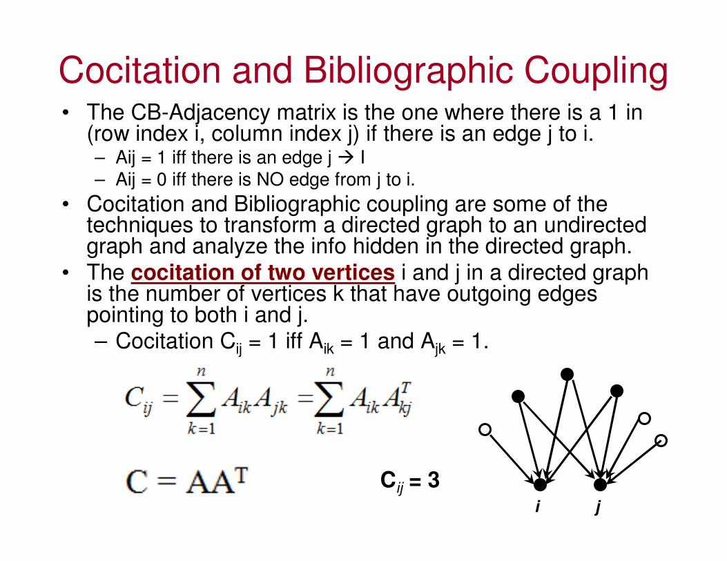
Cocitation and Bibliographic Coupling• The CB-Adjacency matrix is the one where there is a 1 in
(row index i, column index j) if there is an edge j to i.– Aij = 1 iff there is an edge j � I
– Aij = 0 iff there is NO edge from j to i.
• Cocitation and Bibliographic coupling are some of the techniques to transform a directed graph to an undirected graph and analyze the info hidden in the directed graph.
• The cocitation of two vertices i and j in a directed graph is the number of vertices k that have outgoing edges pointing to both i and j. – Cocitation Cij = 1 iff Aik = 1 and Ajk = 1.
i j
Cij = 3
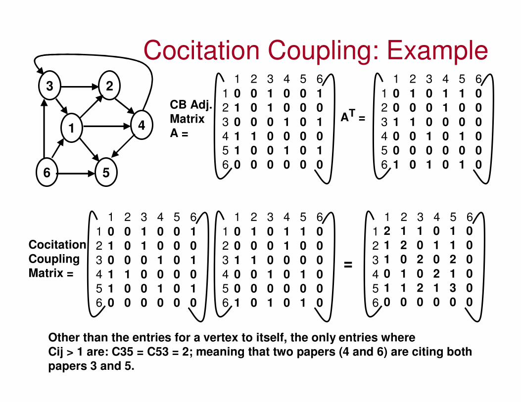
Cocitation Coupling: Example
1
23
4
6 5
1
2
3
4
5
6
1 2 3 4 5 6
0 0 1 0 0 1
1 0 1 0 0 0
0 0 0 1 0 1
1 1 0 0 0 0
1 0 0 1 0 1
0 0 0 0 0 0
CB Adj.
Matrix
A =
1
2
3
4
5
6
1 2 3 4 5 6
0 1 0 1 1 0
0 0 0 1 0 0
1 1 0 0 0 0
0 0 1 0 1 0
0 0 0 0 0 0
1 0 1 0 1 0
AT =
Cocitation
Coupling
Matrix =
1
2
3
4
5
6
1 2 3 4 5 6
=
1
2
3
4
5
6
1 2 3 4 5 6
0 0 1 0 0 1
1 0 1 0 0 0
0 0 0 1 0 1
1 1 0 0 0 0
1 0 0 1 0 1
0 0 0 0 0 0
1
2
3
4
5
6
1 2 3 4 5 6
0 1 0 1 1 0
0 0 0 1 0 0
1 1 0 0 0 0
0 0 1 0 1 0
0 0 0 0 0 0
1 0 1 0 1 0
2 1 1 0 1 0
1 2 0 1 1 0
1 0 2 0 2 0
0 1 0 2 1 0
1 1 2 1 3 0
0 0 0 0 0 0
Other than the entries for a vertex to itself, the only entries whereCij > 1 are: C35 = C53 = 2; meaning that two papers (4 and 6) are citing both
papers 3 and 5.
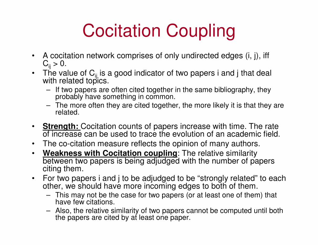
Cocitation Coupling
• A cocitation network comprises of only undirected edges (i, j), iffCij > 0.
• The value of Cij is a good indicator of two papers i and j that deal with related topics.– If two papers are often cited together in the same bibliography, they
probably have something in common.
– The more often they are cited together, the more likely it is that they are related.
• Strength: Cocitation counts of papers increase with time. The rate of increase can be used to trace the evolution of an academic field.
• The co-citation measure reflects the opinion of many authors.
• Weakness with Cocitation coupling: The relative similarity between two papers is being adjudged with the number of papers citing them.
• For two papers i and j to be adjudged to be “strongly related” to each other, we should have more incoming edges to both of them. – This may not be the case for two papers (or at least one of them) that
have few citations.
– Also, the relative similarity of two papers cannot be computed until both the papers are cited by at least one paper.

Bibliographic Coupling• Two papers i and j are related if they refer to one
or more papers k in common.
– The number of common references is an indicator of the
similarity between the two papers.
• However, the similarity is based on the opinion of only the
authors of the two papers; not others in the subject area – a
weakness to assess similarity between two papers.
– It is a static measure: established when a paper gets
published and not updated henceforth.
• Hence, it cannot be used to trace the evolution of an academic
field.
– Strength: Unlike Co-citation coupling, there is no need
to wait for other papers to cite.

Bibliographic Coupling• The bibliographic coupling
of two vertices i and j in a directed graph is the number
of vertices k that have incoming edges from both i and j.
– Bibliographic coupling Bij = 1 iff Aki = 1 and Akj = 1.
i j

Bibliographic Coupling: Example
1
23
4
6 5
1
2
3
4
5
6
1 2 3 4 5 6
0 0 1 0 0 1
1 0 1 0 0 0
0 0 0 1 0 1
1 1 0 0 0 0
1 0 0 1 0 1
0 0 0 0 0 0
CB Adj.
Matrix
A =
1
2
3
4
5
6
1 2 3 4 5 6
0 1 0 1 1 0
0 0 0 1 0 0
1 1 0 0 0 0
0 0 1 0 1 0
0 0 0 0 0 0
1 0 1 0 1 0
AT =
Bibliogr.
Coupling
Matrix =
1
2
3
4
5
6
1 2 3 4 5 6
=
1
2
3
4
5
6
1 2 3 4 5 6
0 0 1 0 0 1
1 0 1 0 0 0
0 0 0 1 0 1
1 1 0 0 0 0
1 0 0 1 0 1
0 0 0 0 0 0
1
2
3
4
5
6
1 2 3 4 5 6
0 1 0 1 1 0
0 0 0 1 0 0
1 1 0 0 0 0
0 0 1 0 1 0
0 0 0 0 0 0
1 0 1 0 1 0
3 1 1 1 0 1
1 1 0 0 0 0
1 0 2 0 0 1
1 0 0 2 0 2
0 0 0 0 0 0
1 0 1 2 0 3
Other than the entries for a vertex to itself, the only entries whereBij > 1 are: B46 = B64 = 2; meaning that two papers (1 and 3) are both being
referred by papers 4 and 6.
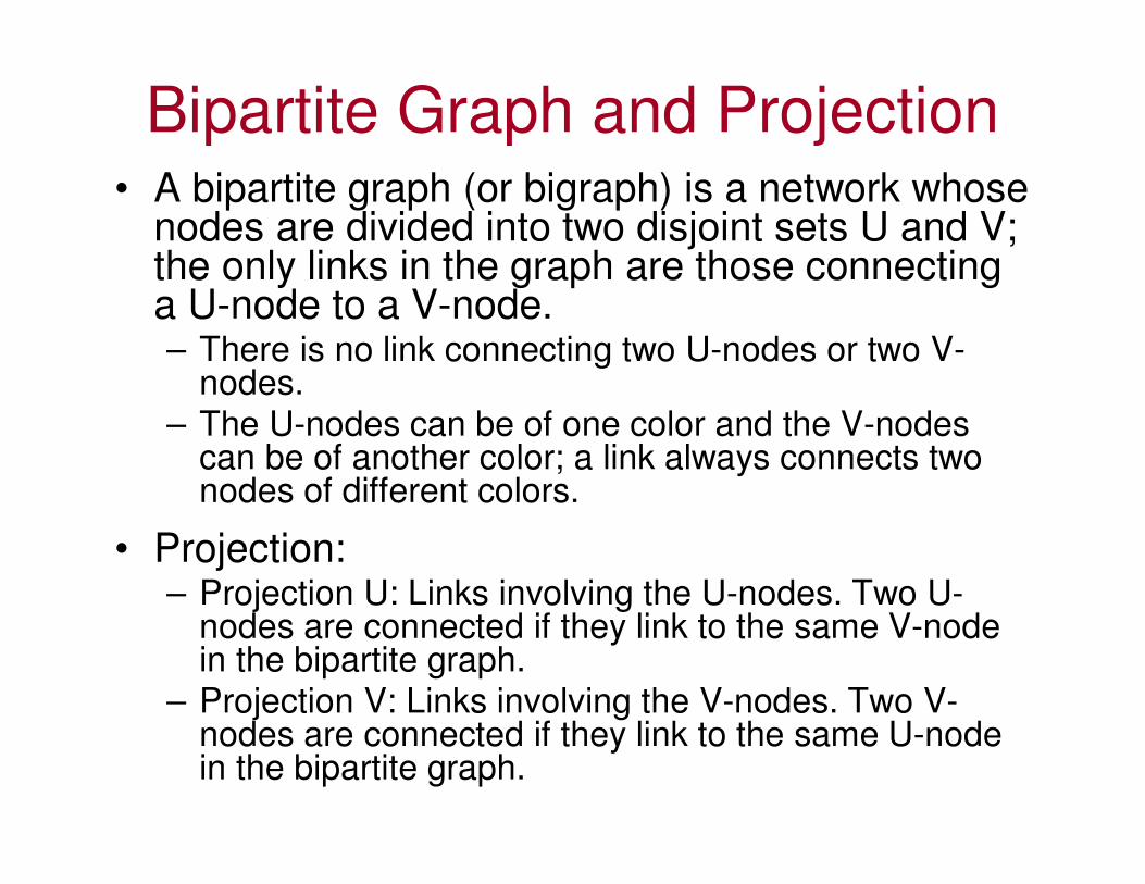
Bipartite Graph and Projection• A bipartite graph (or bigraph) is a network whose
nodes are divided into two disjoint sets U and V; the only links in the graph are those connecting a U-node to a V-node. – There is no link connecting two U-nodes or two V-
nodes.– The U-nodes can be of one color and the V-nodes
can be of another color; a link always connects two nodes of different colors.
• Projection:– Projection U: Links involving the U-nodes. Two U-
nodes are connected if they link to the same V-node in the bipartite graph.
– Projection V: Links involving the V-nodes. Two V-nodes are connected if they link to the same U-node in the bipartite graph.

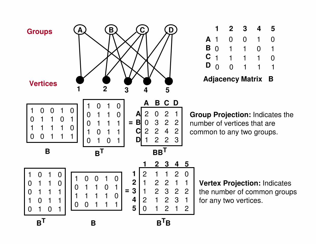
Bipartite Graph and Projection
Source: Fig. 2.9a, Barabasi
(Vertex Projection) (Group Projection)

Incidence Matrix and Projections
Vertex ProjectionTwo vertices are connected if they
belong to at least one common group.
Group ProjectionTwo groups are connected if they
share at least one common vertex.
VPij is the number of groups that
i and j share.
VPii is the number of groups to
which i belongs to.
GPij is the number of vertices that
groups i and j share.
GPii is the number of vertices that
belong to group i.
A B C D
1 2 3 4 5
A
B
C
D
1 2 3 4 5
1 0 0 1 0
0 1 1 0 1
1 1 1 1 0
0 0 1 1 1
1 0 0 1 0
0 1 1 0 1
1 1 1 1 0
0 0 1 1 1
1 0 1 0
0 1 1 0
0 1 1 1
1 0 1 1
0 1 0 1
2 0 2 1
0 3 2 2
2 2 4 2
1 2 2 3
1 0 1 0
0 1 1 0
0 1 1 1
1 0 1 1
0 1 0 1
1 0 0 1 0
0 1 1 0 1
1 1 1 1 0
0 0 1 1 1
2 1 1 2 0
1 2 2 1 1
1 2 3 2 2
2 1 2 3 1
0 1 2 1 2
=
=
Adjacency Matrix B
B BT BBT
BT B BTB
Groups
Vertices
Group Projection: Indicates the
number of vertices that are
common to any two groups.
Vertex Projection: Indicates
the number of common groups
for any two vertices.
A
B
C
D
A B C D
1
2
3
4
5
1 2 3 4 5
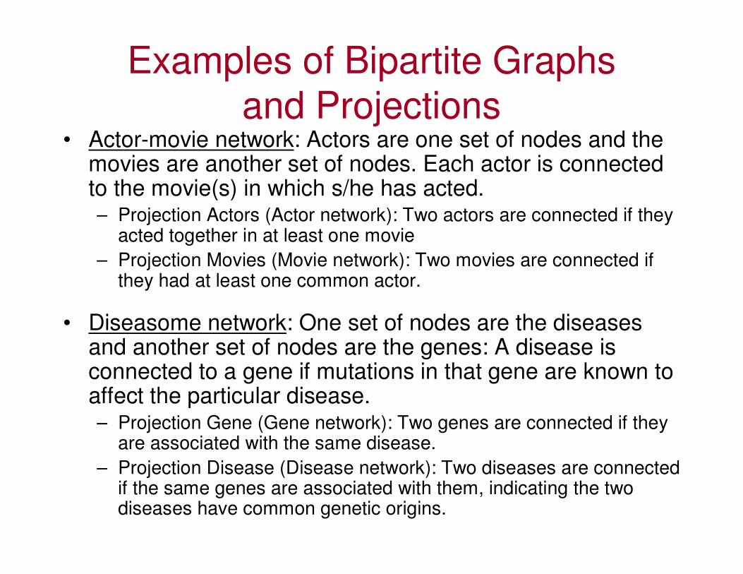
Examples of Bipartite Graphs and Projections
• Actor-movie network: Actors are one set of nodes and the movies are another set of nodes. Each actor is connected to the movie(s) in which s/he has acted.– Projection Actors (Actor network): Two actors are connected if they
acted together in at least one movie
– Projection Movies (Movie network): Two movies are connected if they had at least one common actor.
• Diseasome network: One set of nodes are the diseases and another set of nodes are the genes: A disease is connected to a gene if mutations in that gene are known to affect the particular disease.– Projection Gene (Gene network): Two genes are connected if they
are associated with the same disease.
– Projection Disease (Disease network): Two diseases are connectedif the same genes are associated with them, indicating the two diseases have common genetic origins.
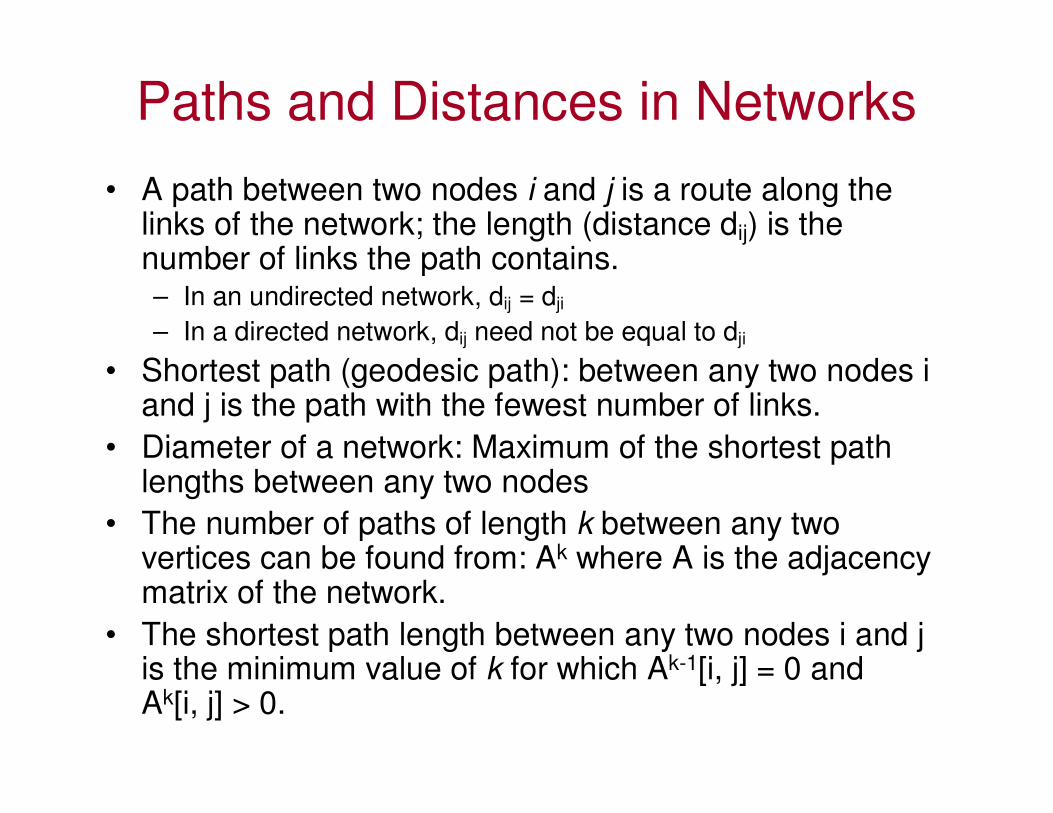
Paths and Distances in Networks
• A path between two nodes i and j is a route along the links of the network; the length (distance dij) is the number of links the path contains.– In an undirected network, dij = dji
– In a directed network, dij need not be equal to dji
• Shortest path (geodesic path): between any two nodes i and j is the path with the fewest number of links.
• Diameter of a network: Maximum of the shortest path lengths between any two nodes
• The number of paths of length k between any two vertices can be found from: Ak where A is the adjacency matrix of the network.
• The shortest path length between any two nodes i and j is the minimum value of k for which Ak-1[i, j] = 0 and Ak[i, j] > 0.

# Walks (Paths) of Certain Length
1 2
3 4
A2 =
1
2
3
4
1 2 3 4
0 1 1 1
1 0 0 1
1 0 0 1
1 1 1 0
1
2
3
4
1 2 3 4
0 1 1 1
1 0 0 1
1 0 0 1
1 1 1 0
1
2
3
4
1 2 3 4
0 1 1 1
1 0 0 1
1 0 0 1
1 1 1 0
1
2
3
4
1 2 3 4
3 1 1 2
1 1 2 1
1 2 2 1
2 1 1 3
=
A Walk is a path in which one or
more vertices (other than the
source and destination) are
repeated.

Number of Paths of Certain Length
1 2
3 4
A2 =
1
2
3
4
1 2 3 4
0 0 0 1
1 0 0 1
1 0 0 0
0 0 1 0
1
2
3
4
1 2 3 4
0 0 1 0
0 0 1 1
0 0 0 1
1 0 0 0
=
1
2
3
4
1 2 3 4
0 0 0 1
1 0 0 1
1 0 0 0
0 0 1 0
1
2
3
4
1 2 3 4
0 0 0 1
1 0 0 1
1 0 0 0
0 0 1 0

Components (Clusters)• The vertices of a graph are said to be in a single
component if there is a path between the vertices.
• A graph is said to be connected if all its vertices are in one single component; otherwise, the graph is said to be disconnected and consists of multiple components.
– Adding one or more links (bridges) can connect the different components
Bridge

Path Terminologies
PathShortest Path
Diameter Cycle
Diameter: Largest shortest path
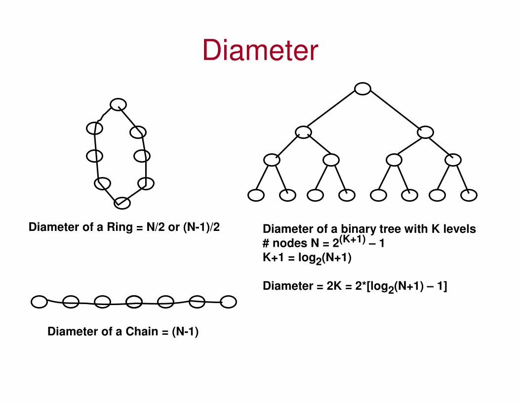
Diameter
Diameter of a Ring = N/2 or (N-1)/2
Diameter of a Chain = (N-1)
Diameter of a binary tree with K levels
# nodes N = 2(K+1) – 1
K+1 = log2(N+1)
Diameter = 2K = 2*[log2(N+1) – 1]
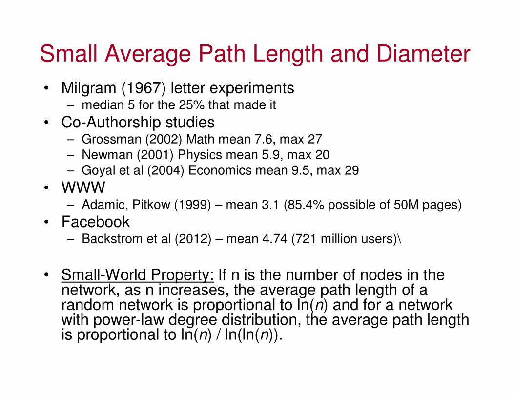
Small Average Path Length and Diameter
• Milgram (1967) letter experiments– median 5 for the 25% that made it
• Co-Authorship studies– Grossman (2002) Math mean 7.6, max 27
– Newman (2001) Physics mean 5.9, max 20
– Goyal et al (2004) Economics mean 9.5, max 29
• WWW– Adamic, Pitkow (1999) – mean 3.1 (85.4% possible of 50M pages)
• Facebook– Backstrom et al (2012) – mean 4.74 (721 million users)\
• Small-World Property: If n is the number of nodes in the network, as n increases, the average path length of a random network is proportional to ln(n) and for a network with power-law degree distribution, the average path length is proportional to ln(n) / ln(ln(n)).
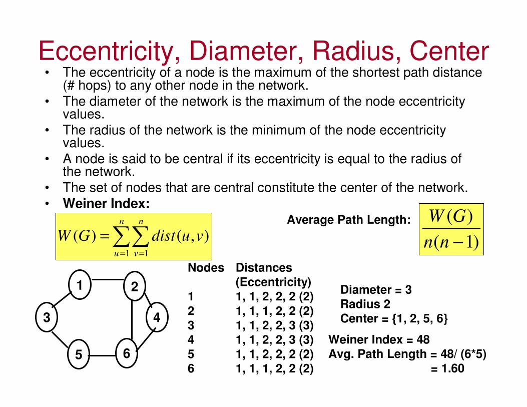
Eccentricity, Diameter, Radius, Center• The eccentricity of a node is the maximum of the shortest path distance
(# hops) to any other node in the network.
• The diameter of the network is the maximum of the node eccentricity values.
• The radius of the network is the minimum of the node eccentricity values.
• A node is said to be central if its eccentricity is equal to the radius of the network.
• The set of nodes that are central constitute the center of the network.
• Weiner Index:
1 2
3 4
5 6
Nodes Distances
(Eccentricity)
1 1, 1, 2, 2, 2 (2)
2 1, 1, 1, 2, 2 (2)
3 1, 1, 2, 2, 3 (3)4 1, 1, 2, 2, 3 (3)5 1, 1, 2, 2, 2 (2)
6 1, 1, 1, 2, 2 (2)
Diameter = 3
Radius 2
Center = {1, 2, 5, 6}
Average Path Length:
Weiner Index = 48Avg. Path Length = 48/ (6*5)
= 1.60
∑∑= =
=n
u
n
v
vudistGW1 1
),()( )1(
)(
−nn
GW

Node Degree vs. EccentricityNode Size (Node Degree)
-Range: 7 to 12
-Larger node size – high degree
-Smaller node size – low degree
Node Color (Node Eccentricity)
-Range: 3 to 4
-White color – low eccentricity
-Dark color – high eccentricity
It is normal to expect nodes
with high degrees to have
low eccentricity and nodes
with low degrees having
high eccentricity.
But, we also see nodes with
high degree having high
eccentricity values, if they are
in the periphery of the network
It makes sense that we do not see nodes with low
degree and low eccentricity. It takes more hops for these nodes to be connected to the other nodes.
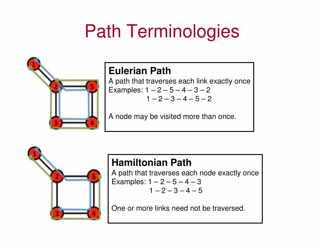
Path Terminologies
Eulerian PathA path that traverses each link exactly once
Examples: 1 – 2 – 5 – 4 – 3 – 2
1 – 2 – 3 – 4 – 5 – 2
A node may be visited more than once.
Hamiltonian PathA path that traverses each node exactly once
Examples: 1 – 2 – 5 – 4 – 3
1 – 2 – 3 – 4 – 5
One or more links need not be traversed.
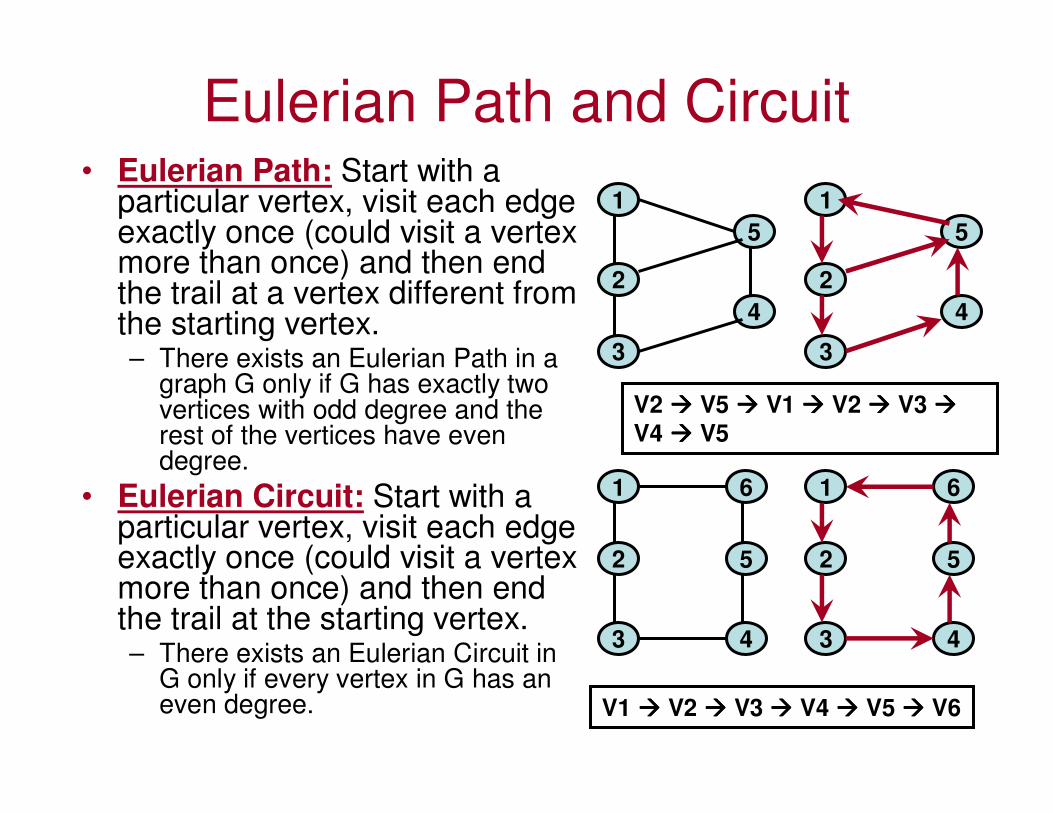
Eulerian Path and Circuit• Eulerian Path: Start with a
particular vertex, visit each edge exactly once (could visit a vertex more than once) and then end the trail at a vertex different from the starting vertex.– There exists an Eulerian Path in a
graph G only if G has exactly two vertices with odd degree and the rest of the vertices have even degree.
• Eulerian Circuit: Start with a particular vertex, visit each edge exactly once (could visit a vertex more than once) and then end the trail at the starting vertex.– There exists an Eulerian Circuit in
G only if every vertex in G has an even degree.
1
2
3
5
4
1
2
3
5
4
V2 ���� V5 ���� V1 ���� V2 ���� V3 ����
V4 ���� V5
1
2
3
6
5
4
1
2
3
6
5
4
V1 ���� V2 ���� V3 ���� V4 ���� V5 ���� V6
Depth First Search (DFS)• Visits graph’s vertices (also called nodes) by always moving away
from last visited vertex to unvisited one, backtracks if there is no adjacent unvisited vertex.
• Break any tie to visit an adjacent vertex, by visiting the vertex with the lowest ID or the lowest alphabet (label).
• Uses a stack
– a vertex is pushed onto the stack when it’s visited for the first time
–a vertex is popped off the stack when it becomes a dead end, i.e., when there is no adjacent unvisited vertex
• “Redraws” graph in tree-like fashion (with tree edges andback edges for undirected graph):
– Whenever a new unvisited vertex is reached for the first time, it is attached as a child to the vertex from which it is being reached. Such an edge is called a tree edge.
– While exploring the neighbors of a vertex, it the algorithm encounters an edge leading to a previously visited vertex other than its immediate predecessor (i.e., its parent in the tree), such an edge is called a back edge.
– The leaf nodes have no children; the root node and other intermediate nodes have one more child.
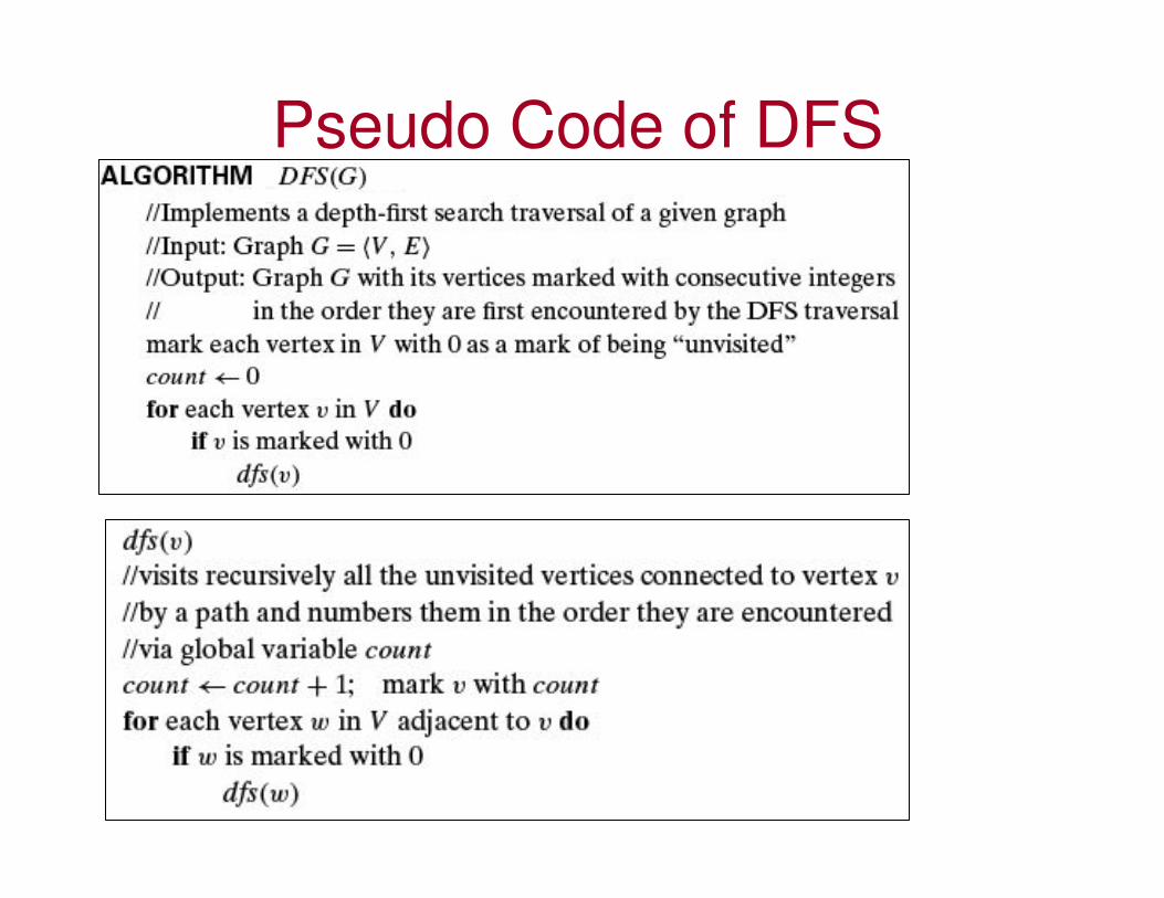
Pseudo Code of DFS
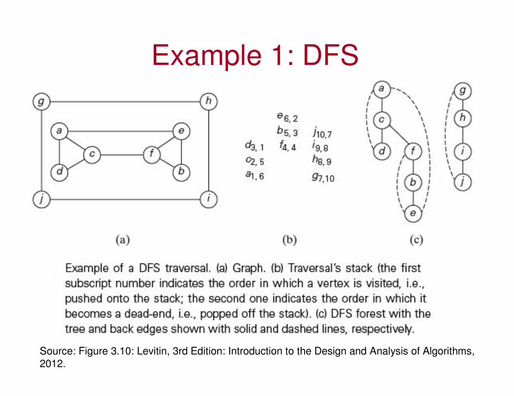
Example 1: DFS
Source: Figure 3.10: Levitin, 3rd Edition: Introduction to the Design and Analysis of Algorithms,
2012.
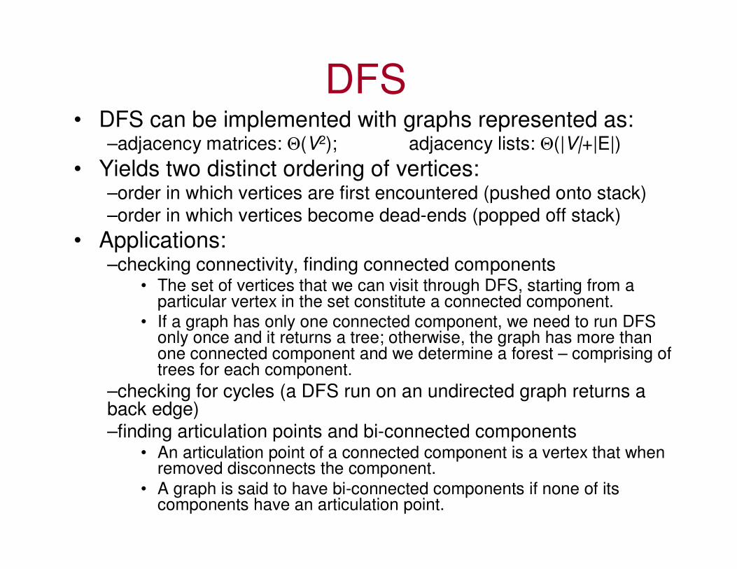
DFS• DFS can be implemented with graphs represented as:
–adjacency matrices: Θ(V2); adjacency lists: Θ(|V|+|E|)
• Yields two distinct ordering of vertices:–order in which vertices are first encountered (pushed onto stack)
–order in which vertices become dead-ends (popped off stack)
• Applications:–checking connectivity, finding connected components
• The set of vertices that we can visit through DFS, starting from a particular vertex in the set constitute a connected component.
• If a graph has only one connected component, we need to run DFS only once and it returns a tree; otherwise, the graph has more than one connected component and we determine a forest – comprising of trees for each component.
–checking for cycles (a DFS run on an undirected graph returns a back edge)
–finding articulation points and bi-connected components• An articulation point of a connected component is a vertex that when
removed disconnects the component.
• A graph is said to have bi-connected components if none of its components have an articulation point.

Example 2: DFS
f b c g
d a e
f b c g
d a e
1, 7
2, 3
3, 2
4, 1 5, 6 6, 5
7, 4
Tree Edge
Back Edge
• Notes on Articulation Point– The root of a DFS tree is an articulation point if it has more than
one child connected through a tree edge. (In the above DFS tree,the root node ‘a’ is an articulation point)
– The leaf nodes of a DFS tree are not articulation points.
– Any other internal vertex v in the DFS tree, if it has one or more sub trees rooted at a child (at least one child node) of v that does NOT have an edge which climbs ’higher ’ than v (through a back edge), then v is an articulation point.
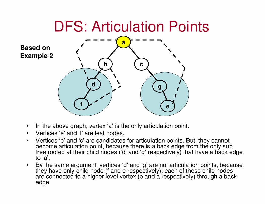
DFS: Articulation Points
• In the above graph, vertex ‘a’ is the only articulation point.
• Vertices ‘e’ and ‘f’ are leaf nodes.
• Vertices ‘b’ and ‘c’ are candidates for articulation points. But, they cannot become articulation point, because there is a back edge from the only sub tree rooted at their child nodes (‘d’ and ‘g’ respectively) that have a back edge to ‘a’.
• By the same argument, vertices ‘d’ and ‘g’ are not articulation points, because they have only child node (f and e respectively); each of these child nodes are connected to a higher level vertex (b and a respectively) through a back edge.
a
b c
d
f
g
e
Based on
Example 2
Example 3: DFS and Articulation Points
f b c g
d a e
f b c g
d a e
1, 7
2, 3
3, 2
4, 1 5, 6 6, 5
7, 4
Tree Edge
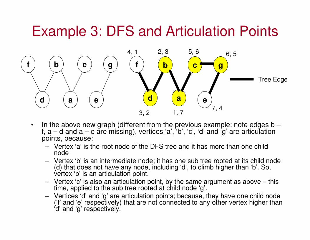
• In the above new graph (different from the previous example: note edges b –f, a – d and a – e are missing), vertices ‘a’, ‘b’, ‘c’, ‘d’ and ‘g’ are articulation points, because:– Vertex ‘a’ is the root node of the DFS tree and it has more than one child
node– Vertex ‘b’ is an intermediate node; it has one sub tree rooted at its child node
(d) that does not have any node, including ‘d’, to climb higher than ‘b’. So, vertex ‘b’ is an articulation point.
– Vertex ‘c’ is also an articulation point, by the same argument as above – this time, applied to the sub tree rooted at child node ‘g’.
– Vertices ‘d’ and ‘g’ are articulation points; because, they have one child node (‘f’ and ‘e’ respectively) that are not connected to any other vertex higher than ‘d’ and ‘g’ respectively.

Example 4: DFS and Articulation Points
f b c g
d a e
f b c g
d a e
1, 7
2, 3
3, 2
4, 1 5, 6 6, 5
7, 4
Tree Edge
• In the above new graph (different from the previous example: note edge a – e and b – f are added back; but a – d is missing):– Vertices ‘a’ and ‘b’ are
articulation points
– Vertex ‘c’ is not an articulation point
Back Edge
a
b c
d
f
g
e
Example 5: DFS and Articulation Points
a
b
c
d e
f g
h
i j
k
a
b
c
d e
f g
h
i j
k
DFS TREE

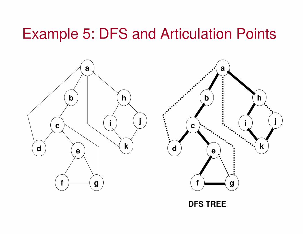
1) Root Vertex ‘a’ has more than one child; so, it is an articulation point.2) Vertices ‘d’, ‘g’ and ‘j’ are leaf nodes3) Vertex ‘b’ is not an articulation point becausethe only sub tree rooted at its child node ‘c’ hasa back edge to a vertex higher than ‘b’ (in thiscase to the root vertex ‘a’)4) Vertex ‘c’ is an articulation point. One of itschild vertex ‘d’ does not have any sub tree rooted at it. The other vertex ‘e’ has a sub tree rooted at it and this sub tree has noback edge higher up than ‘c’. 5) By argument (4), it follows that vertex ‘e’is not an articulation point because the sub treerooted at its child node ‘f’ has a back edge higherup than ‘e’ (to vertex ‘c’); 6) Vertices ‘f’ and ‘k’ are not articulation points becausethey have only one child node each and the child nodesare connected to a vertex higher above ‘f’ and ‘k’.7) Vertex ‘i’ is not an articulation point because the only sub tree rooted at its child has a back edge higher up (to vertices ‘a’ and ‘h’). 8) Vertex ‘h’ is not an articulation point because the only sub tree rooted at ‘h’ has a back edge higher up (to the root vertex ‘a’).
Identification of the Articulation Points of the Graph in Example 5
a
b
c
d e
f g
h
i j
k
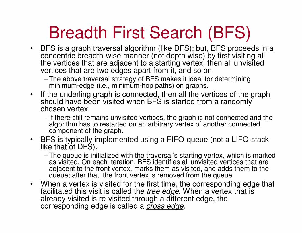
Breadth First Search (BFS)• BFS is a graph traversal algorithm (like DFS); but, BFS proceeds in a
concentric breadth-wise manner (not depth wise) by first visiting all the vertices that are adjacent to a starting vertex, then all unvisited vertices that are two edges apart from it, and so on.– The above traversal strategy of BFS makes it ideal for determining
minimum-edge (i.e., minimum-hop paths) on graphs.
• If the underling graph is connected, then all the vertices of the graph should have been visited when BFS is started from a randomly chosen vertex. – If there still remains unvisited vertices, the graph is not connected and the
algorithm has to restarted on an arbitrary vertex of another connected component of the graph.
• BFS is typically implemented using a FIFO-queue (not a LIFO-stack like that of DFS).– The queue is initialized with the traversal’s starting vertex, which is marked
as visited. On each iteration, BFS identifies all unvisited vertices that are adjacent to the front vertex, marks them as visited, and adds them to the queue; after that, the front vertex is removed from the queue.
• When a vertex is visited for the first time, the corresponding edge that facilitated this visit is called the tree edge. When a vertex that is already visited is re-visited through a different edge, the corresponding edge is called a cross edge.
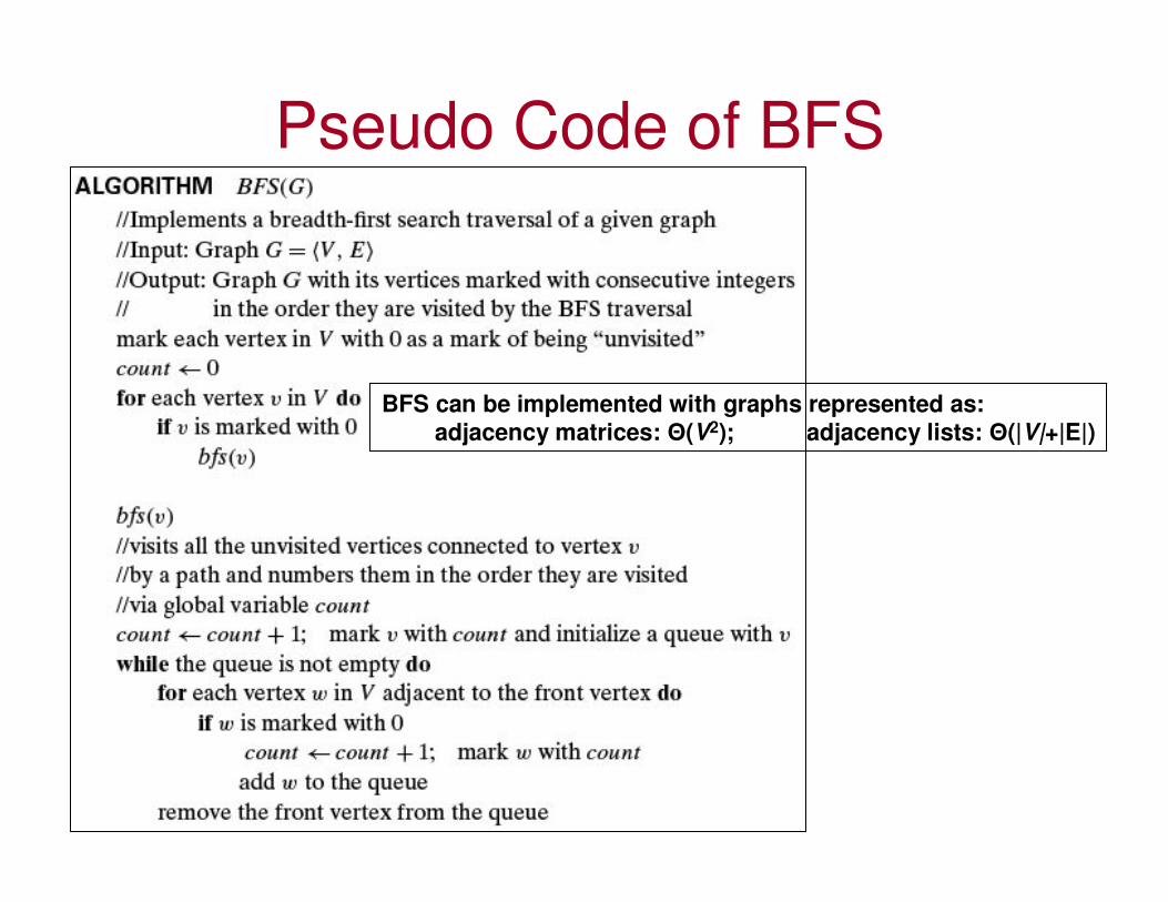
Pseudo Code of BFS
BFS can be implemented with graphs represented as:adjacency matrices: Θ(V2); adjacency lists: Θ(|V|+|E|)
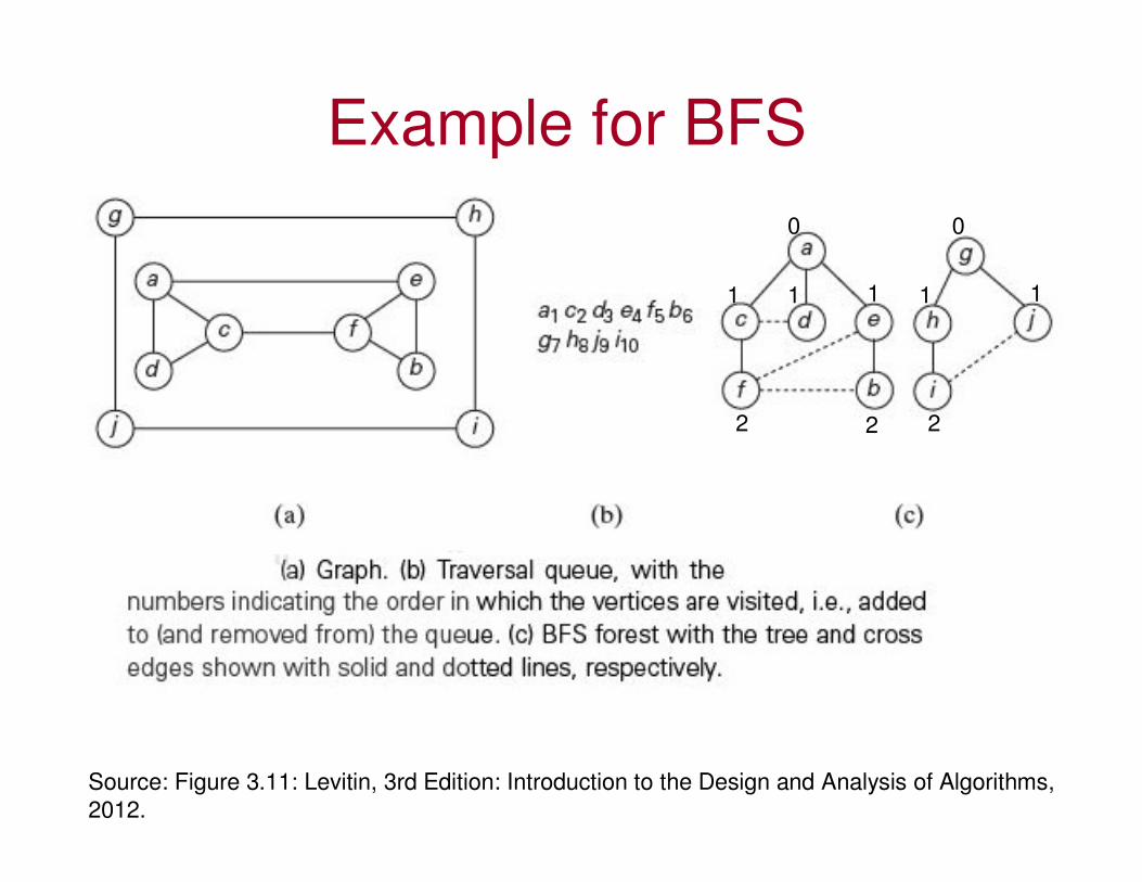
Example for BFS
Source: Figure 3.11: Levitin, 3rd Edition: Introduction to the Design and Analysis of Algorithms,
2012.
0
1 1 1
2 2
0
1 1
2
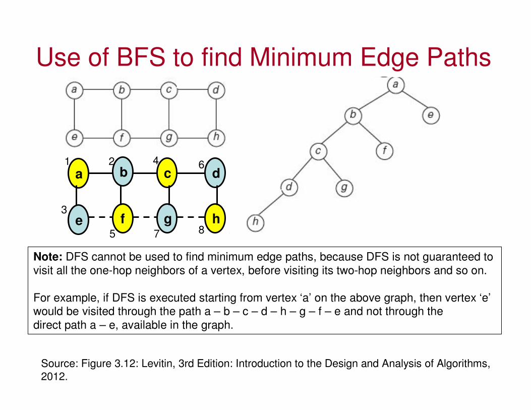
Use of BFS to find Minimum Edge Paths
Source: Figure 3.12: Levitin, 3rd Edition: Introduction to the Design and Analysis of Algorithms,
2012.
Note: DFS cannot be used to find minimum edge paths, because DFS is not guaranteed to visit all the one-hop neighbors of a vertex, before visiting its two-hop neighbors and so on.
For example, if DFS is executed starting from vertex ‘a’ on the above graph, then vertex ‘e’would be visited through the path a – b – c – d – h – g – f – e and not through the direct path a – e, available in the graph.
a b c d
e f g h
1 2
3
5
4
7
6
8

Comparison of DFS and BFS
Source: Table 3.1: Levitin, 3rd Edition: Introduction to the Design and Analysis of Algorithms,
2012.
With the levels of a tree, referenced starting from the root node, A back edge in a DFS tree could connect vertices at different levels; whereas, a cross edgein a BFS tree always connects vertices that are either at the same level or at adjacent levels.
There is always only a unique ordering of the vertices, according to BFS, in the order they are visited (added and removed from the queue in the same order). On the other hand, with DFS – vertices could be ordered in the order they are added to the Stack, typically different from the order in which they are removed from the stack.
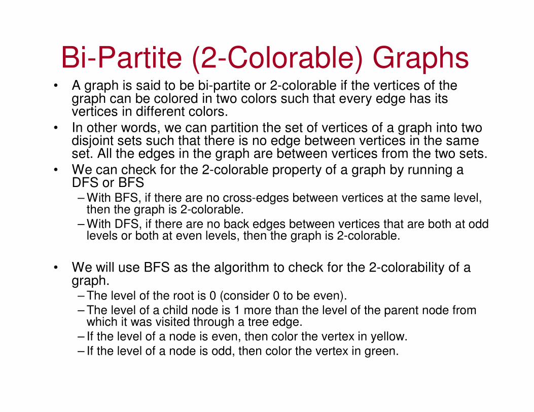
Bi-Partite (2-Colorable) Graphs • A graph is said to be bi-partite or 2-colorable if the vertices of the
graph can be colored in two colors such that every edge has its vertices in different colors.
• In other words, we can partition the set of vertices of a graph into two disjoint sets such that there is no edge between vertices in the same set. All the edges in the graph are between vertices from the two sets.
• We can check for the 2-colorable property of a graph by running a DFS or BFS– With BFS, if there are no cross-edges between vertices at the same level,
then the graph is 2-colorable.
– With DFS, if there are no back edges between vertices that are both at odd levels or both at even levels, then the graph is 2-colorable.
• We will use BFS as the algorithm to check for the 2-colorability of a graph.– The level of the root is 0 (consider 0 to be even).
– The level of a child node is 1 more than the level of the parent node from which it was visited through a tree edge.
– If the level of a node is even, then color the vertex in yellow.
– If the level of a node is odd, then color the vertex in green.

Bi-Partite (2-Colorable) Graphs
a b c
d e f
a b c
d e f
0 1
1
2
2 3
a b c
d e f
Example for a 2-Colorable Graph
a b
d e
Example for a Graph that is Not 2-Colorable
a b
d e
0 1
1 1
We encounter cross edges between vertices
b and e; d and e – all the three vertices are
in the same level.
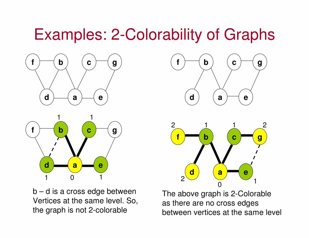
Examples: 2-Colorability of Graphs
f b c g
d a e
f b c g
d a e
01
1
1
1
b – d is a cross edge between
Vertices at the same level. So,
the graph is not 2-colorable
f b c g
d a e
f b c g
d a e
0
11
1
2
2
2
The above graph is 2-Colorable
as there are no cross edges
between vertices at the same level
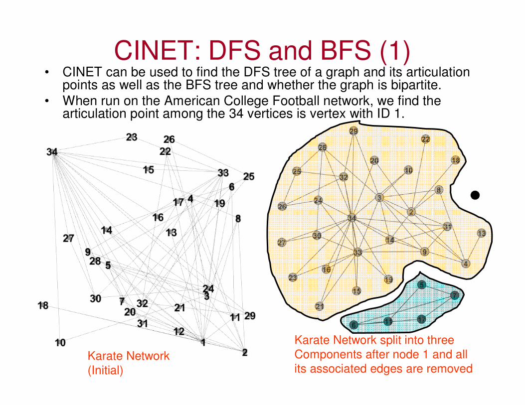
CINET: DFS and BFS (1)• CINET can be used to find the DFS tree of a graph and its articulation
points as well as the BFS tree and whether the graph is bipartite.
• When run on the American College Football network, we find the articulation point among the 34 vertices is vertex with ID 1.
Karate Network
(Initial)
Karate Network split into three
Components after node 1 and all
its associated edges are removed
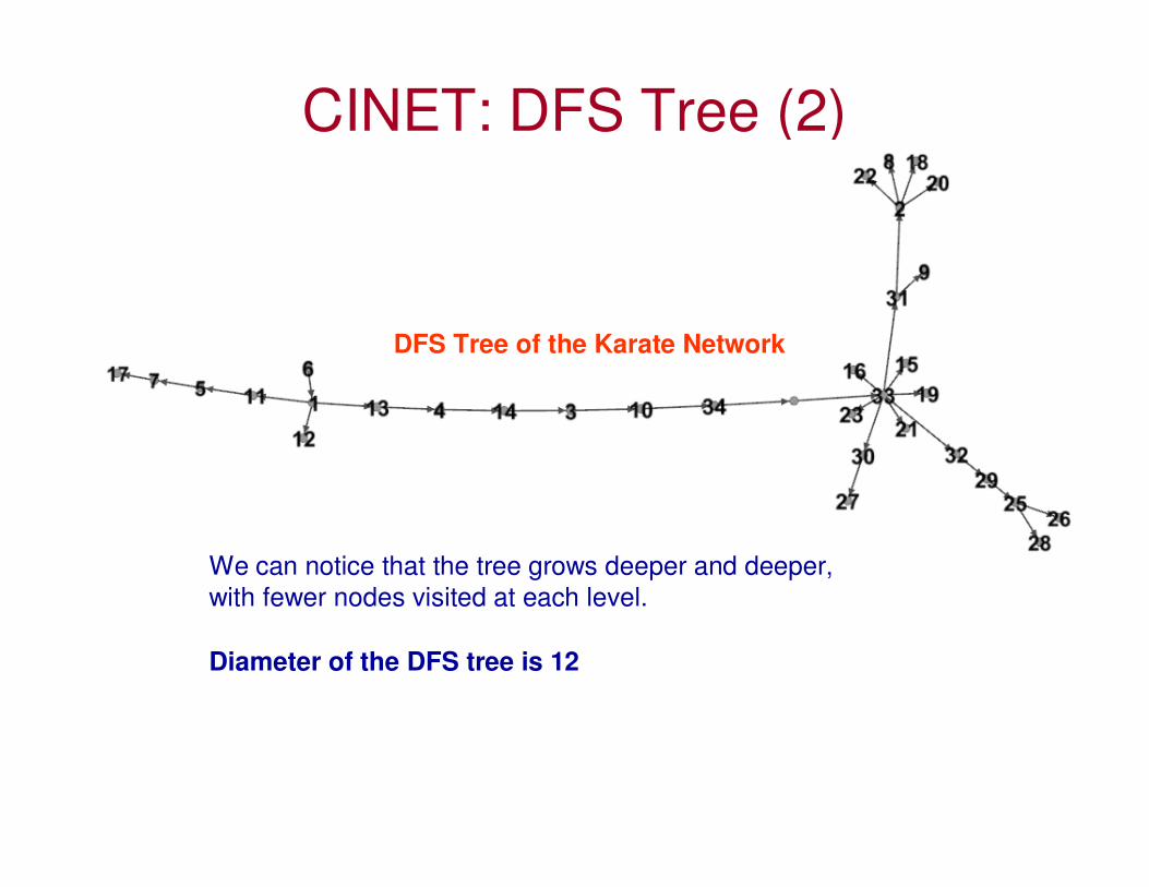
CINET: DFS Tree (2)
DFS Tree of the Karate Network
We can notice that the tree grows deeper and deeper,
with fewer nodes visited at each level.
Diameter of the DFS tree is 12
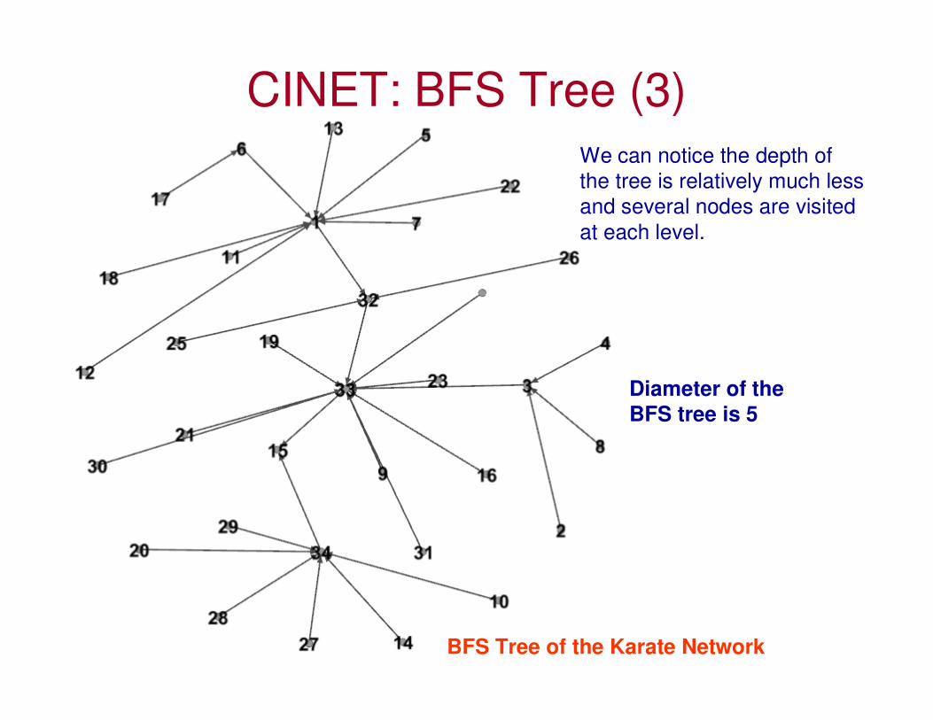
CINET: BFS Tree (3)
BFS Tree of the Karate Network
We can notice the depth of
the tree is relatively much less
and several nodes are visited
at each level.
Diameter of the
BFS tree is 5

Directed Acyclic Graphs (DAGs)• A directed graph with no cycles.
– E.g., Citation network: we always cite the work done earlier. A prior work does not cite a work to be done later.
• In a DAG, there must be at least one vertex that has only all incoming edges and no outgoing edge.– We start with one vertex, go around the vertices in the graph. If the
path never reaches a vertex with no outgoing edges, then it musteventually arrive back at a vertex that has been visited previously –at most we can visit all the n vertices in the graph once before the path either terminates or we are forced to revisit a vertex (in the latter case, we encounter a cycle).
• To test for cycle: Remove the vertices with no outgoing edges (and all the associated incoming edges), one by one. If there is a cycle, there will be a scenario in which we could not find any vertex without outgoing edges.– If all vertices could be removed one by one, the graph is acyclic.
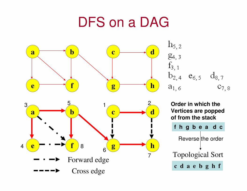
DFS on a DAG
a b
e f
c d
g h
a b
e f
c d
g h
Forward edgeTopological Sort
c d a e b g h f
f h g b e a d c
Order in which the
Vertices are popped
of from the stack
Reverse the order
Cross edge
1 23
4
5
67
8

DFS on a DAG
a b
e f
c d
g h
1 23
4
5
67
8
1
2
3
4
5
6
7
8
1 2 3 4 5 6 7 8
0 1 0 0 0 1 0 0
0 0 0 0 0 0 1 00 0 0 1 1 0 0 1
0 0 0 0 0 0 0 10 0 0 0 0 1 0 1
0 0 0 0 0 0 1 0
0 0 0 0 0 0 0 0
0 0 0 0 0 0 0 0
Let the vertices be numbered in the order
in which they are topologically sort.
An adjacency matrix of the vertices listed in
the order of their topological sort is strictly
upper triangular.

Components• Component: The subset of vertices in a graph that are
reachable from one another through paths of length one or more.
• Maximal subset property of a component: Inclusion of additional edges or vertices from the graph to this subset will break the connectivity of a component.
• A graph in which all its vertices are not in one component is said to be disconnected. – Undirected graph: The set of all vertices that are reachable (via
BFS or DFS) starting from a particular vertex are all said to be in the same component.
– Directed graph: • Weakly connected: The vertices of a di-graph are said to form a
weakly connected component if they are connected in their undirected version.
• Strongly connected: The vertices of a di-graph are said to form a strongly connected component if they are connected (reachable from each other through paths).
– A standalone vertex that is not reachable to and from any other vertex is said to be in its own component.
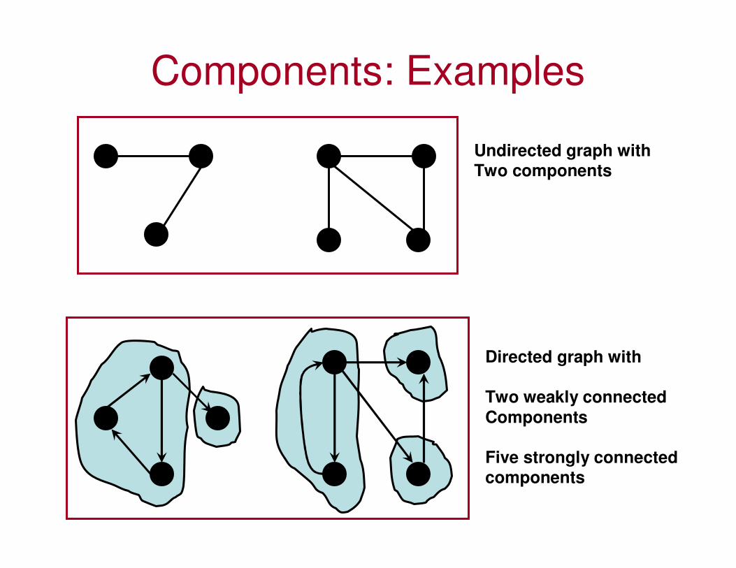
Components: Examples
Undirected graph with
Two components
Directed graph with
Two weakly connected
Components
Five strongly connected
components

Components in a DAG• Note that for a directed graph to have a
strongly connected component (scc), the
graph should have a cycle: because, we
need the vertices in an scc to be reachable
from one another.
– There has to be a path from A to B through a sequence of edges and vice-versa through a different sequence of edges.
• Hence, there cannot be a strongly
connected component in a DAG.

Out- and In- Components• The out-component (defined for a
specific vertex A) in a directed graph is the set of all vertices (including A itself) that are reachable from A through one or more paths.
• The in-component (defined for a specific vertex A) in a directed graph is the set of all vertices (including A itself) that have a directed path to A.
• The intersection of both the out-component and in-component of A yields a strongly connected component (scc) involving vertex A. All the vertices in such a scc are reachable from each other at least through A.
A
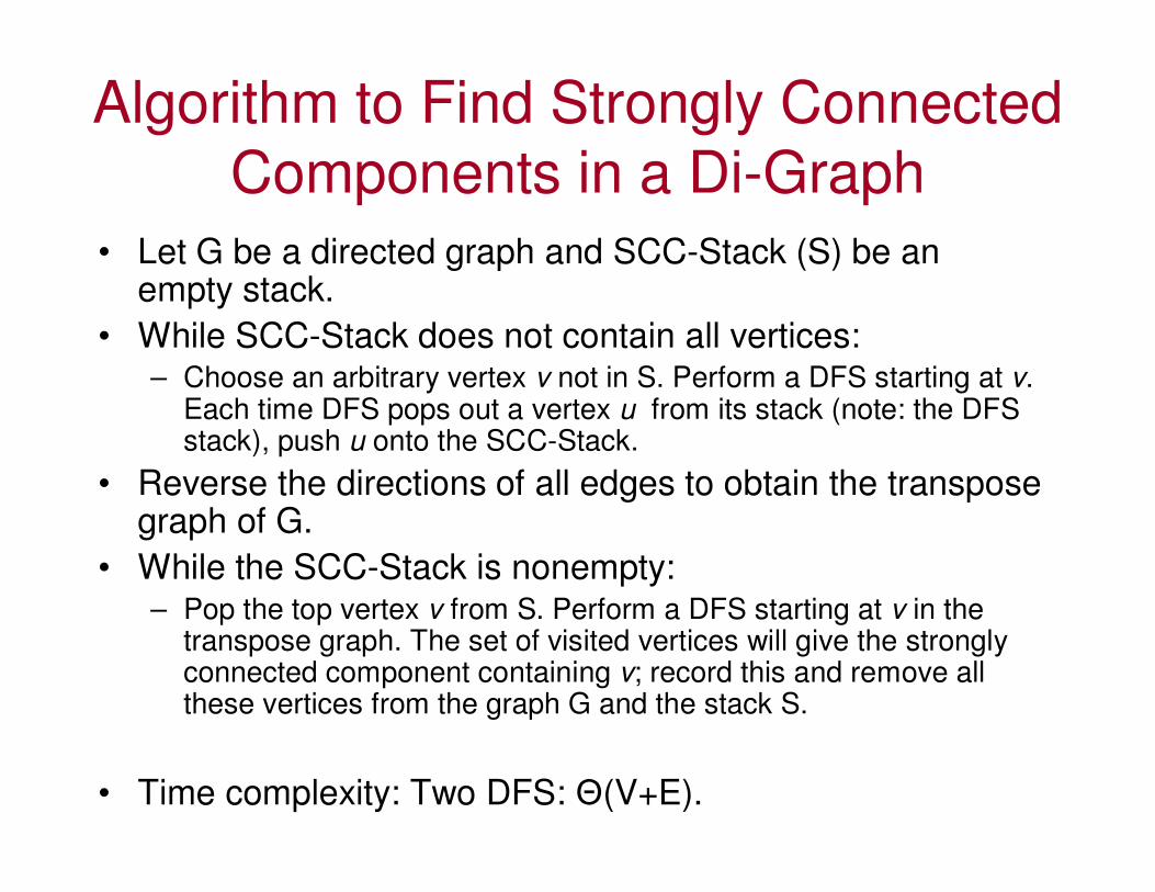
Algorithm to Find Strongly Connected Components in a Di-Graph
• Let G be a directed graph and SCC-Stack (S) be an empty stack.
• While SCC-Stack does not contain all vertices:– Choose an arbitrary vertex v not in S. Perform a DFS starting at v.
Each time DFS pops out a vertex u from its stack (note: the DFS stack), push u onto the SCC-Stack.
• Reverse the directions of all edges to obtain the transpose graph of G.
• While the SCC-Stack is nonempty:– Pop the top vertex v from S. Perform a DFS starting at v in the
transpose graph. The set of visited vertices will give the strongly connected component containing v; record this and remove all these vertices from the graph G and the stack S.
• Time complexity: Two DFS: Θ(V+E).
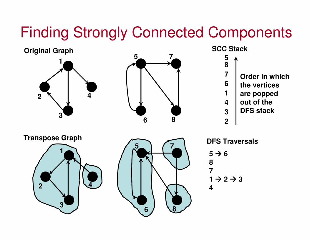
Finding Strongly Connected Components
1
2
3
4
5
6
7
8
SCC Stack
2
3
4
1
6
7
85
Order in which
the vertices
are popped
out of the
DFS stack
1
2
3
4
5
6
7
8
5 ���� 6
8
7
1 ���� 2 ���� 3
4
Transpose Graph
Original Graph
DFS Traversals

Giant Component
• The largest component encompasses a significant fraction of the graph.
• Even as the network size grows to infinity, the giant component occupies a finite fraction of the network.
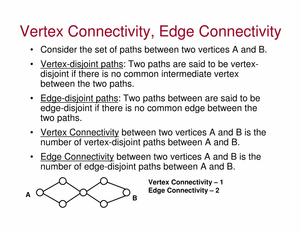
Vertex Connectivity, Edge Connectivity• Consider the set of paths between two vertices A and B.
• Vertex-disjoint paths: Two paths are said to be vertex-disjoint if there is no common intermediate vertex between the two paths.
• Edge-disjoint paths: Two paths between are said to be edge-disjoint if there is no common edge between the two paths.
• Vertex Connectivity between two vertices A and B is the number of vertex-disjoint paths between A and B.
• Edge Connectivity between two vertices A and B is the number of edge-disjoint paths between A and B.
AB
Vertex Connectivity – 1
Edge Connectivity – 2
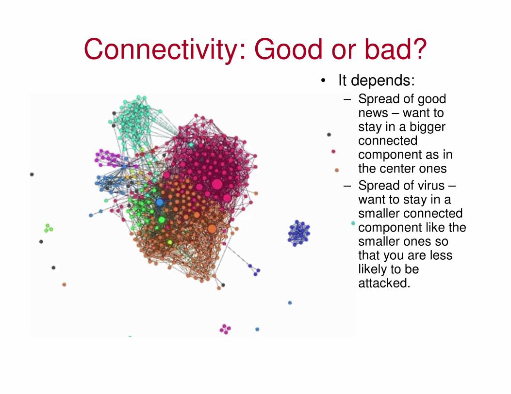
Connectivity: Good or bad?• It depends:
– Spread of good news – want to stay in a bigger connected component as in the center ones
– Spread of virus –want to stay in a smaller connected component like the smaller ones so that you are less likely to be attacked.
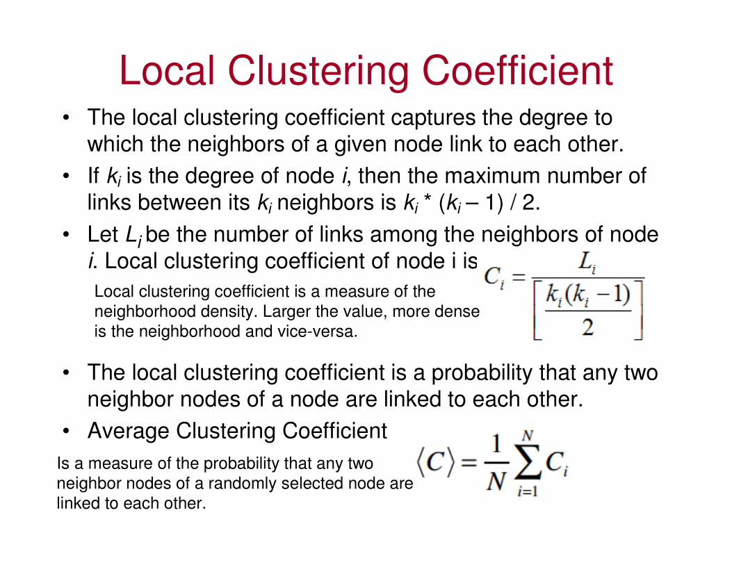
Local Clustering Coefficient• The local clustering coefficient captures the degree to
which the neighbors of a given node link to each other.
• If ki is the degree of node i, then the maximum number of
links between its ki neighbors is ki * (ki – 1) / 2.
• Let Li be the number of links among the neighbors of node
i. Local clustering coefficient of node i is
• The local clustering coefficient is a probability that any two
neighbor nodes of a node are linked to each other.
• Average Clustering Coefficient
Is a measure of the probability that any two
neighbor nodes of a randomly selected node are
linked to each other.
Local clustering coefficient is a measure of the
neighborhood density. Larger the value, more dense
is the neighborhood and vice-versa.

Examples for Local Clustering Coefficients
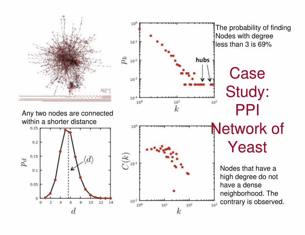
Case Study:
PPI Network of
Yeast
The probability of finding
Nodes with degree
less than 3 is 69%
Any two nodes are connected
within a shorter distance
Nodes that have a
high degree do not
have a dense
neighborhood. The
contrary is observed.

CINET: Degree vs. Clustering Coeff.(1)American College
Football NetworkThe larger the node size, the higher
the node degree.
The darker a node, the higher
its clustering coefficient.
Avg. Node Degree = 10.4
Avg. cluster coeff. = 0.4
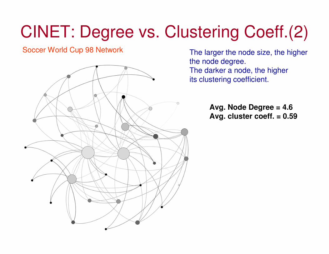
CINET: Degree vs. Clustering Coeff.(2)Soccer World Cup 98 Network The larger the node size, the higher
the node degree.
The darker a node, the higher
its clustering coefficient.
Avg. Node Degree = 4.6
Avg. cluster coeff. = 0.59

Network Types: Terminologies• Complement of a network G: Is a network comprising of all the
nodes in G but comprising of links (between nodes) that are not in G.
• Regular network: An r-regular network is a network in which each node has degree r and such a network of n nodes has rn/2 links.
• Complete network: comprises of links between any two nodes
• Empty network: Complement of a complete network
• K-Colorability: A network is k-colorable if for any link in the network, the end vertices are colored in different colors, chosen among the k colors.
• Bipartite networks: The network is partitioned to two disjoint (non-empty) subsets V1 and V2 such that V1 U V2 = V, the set of all vertices and the only edges in the network are those that connect a vertex in V1 to a vertex in V2.– There are no edges between any two vertices within V1 or V2.
• Planar Networks: The network can be drawn in such a way (in a plane) that no two edges intersect (except at the end nodes).
• K-partite networks: The network is partitioned into k-disjoint subsets; such that any edge in the network is between the vertices acrossany two of these subsets.
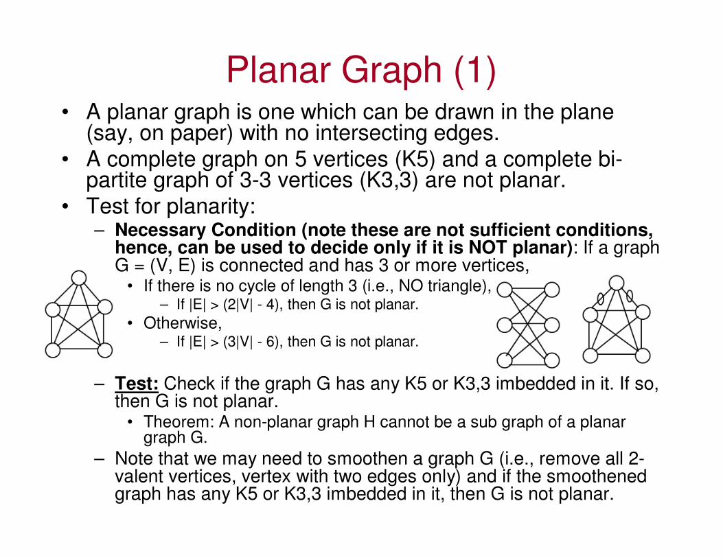
Planar Graph (1)• A planar graph is one which can be drawn in the plane
(say, on paper) with no intersecting edges.
• A complete graph on 5 vertices (K5) and a complete bi-partite graph of 3-3 vertices (K3,3) are not planar.
• Test for planarity:– Necessary Condition (note these are not sufficient conditions,
hence, can be used to decide only if it is NOT planar): If a graph G = (V, E) is connected and has 3 or more vertices,
• If there is no cycle of length 3 (i.e., NO triangle), – If |E| > (2|V| - 4), then G is not planar.
• Otherwise,– If |E| > (3|V| - 6), then G is not planar.
– Test: Check if the graph G has any K5 or K3,3 imbedded in it. If so, then G is not planar.
• Theorem: A non-planar graph H cannot be a sub graph of a planar graph G.
– Note that we may need to smoothen a graph G (i.e., remove all 2-valent vertices, vertex with two edges only) and if the smoothened graph has any K5 or K3,3 imbedded in it, then G is not planar.

Planar Graph (2)
After
Smoothening
After
Smoothening
NOT PLANAR
NOT PLANAR
10 vertices, 18 edges
18 > 3 (10) – 6;
Passes test for necess. condition
10 vertices, 13 edges
13 > 2 (10) - 4. Fails test for necess. condition
there is a cycle of length 3
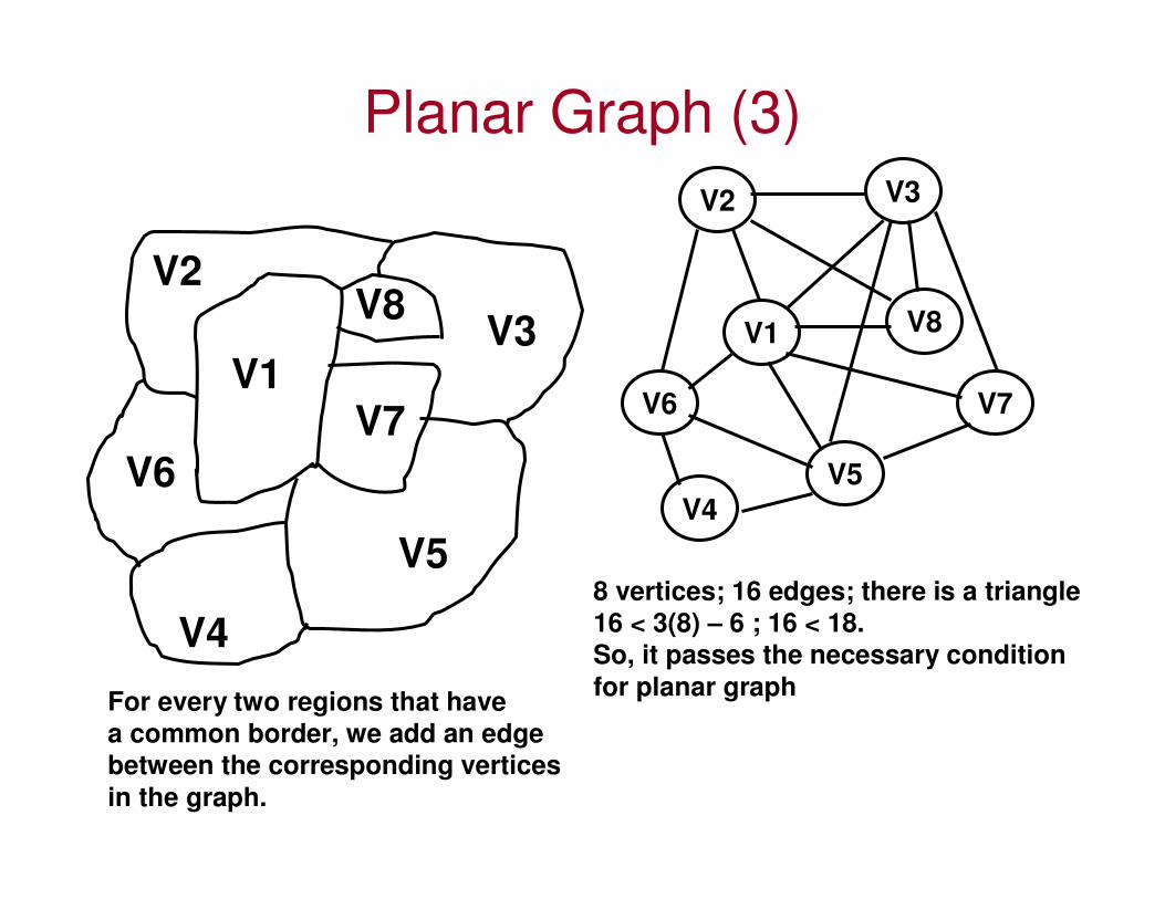
Planar Graph (3)
V1
V2
V3
V4
V5
V6
V2 V3
V7
V8V1 V8
V6 V7
V5
V4
8 vertices; 16 edges; there is a triangle
16 < 3(8) – 6 ; 16 < 18.
So, it passes the necessary condition
for planar graphFor every two regions that have
a common border, we add an edge
between the corresponding vertices
in the graph.

Planar Graph (4)V2 V3
V1 V8
V6 V7
V5
V4
V2 V3
V1 V8
V6 V7
V5
V6
V7
V8
V2
V5
V1
After smoothing,
among the remaining 7
vertices, there cannot be
a K5 because there are
three vertices V6, V7 and
V8 of degree less than 4.
V3
Among the remaining 7
vertices, V6, V7 and V8
are the three vertices that
do not have any edge
between them. There are
edges V2 – V5; V2 – V1;
V2 – V3; V1 – V5. Hence,
{V6, V7, V8} are the onlyDisjoint subset; there cannot be another
disjoint subset.
After
Smoothing
There is NO K5 and
NO K3, 3.
Hence, the graph is
PLANAR.
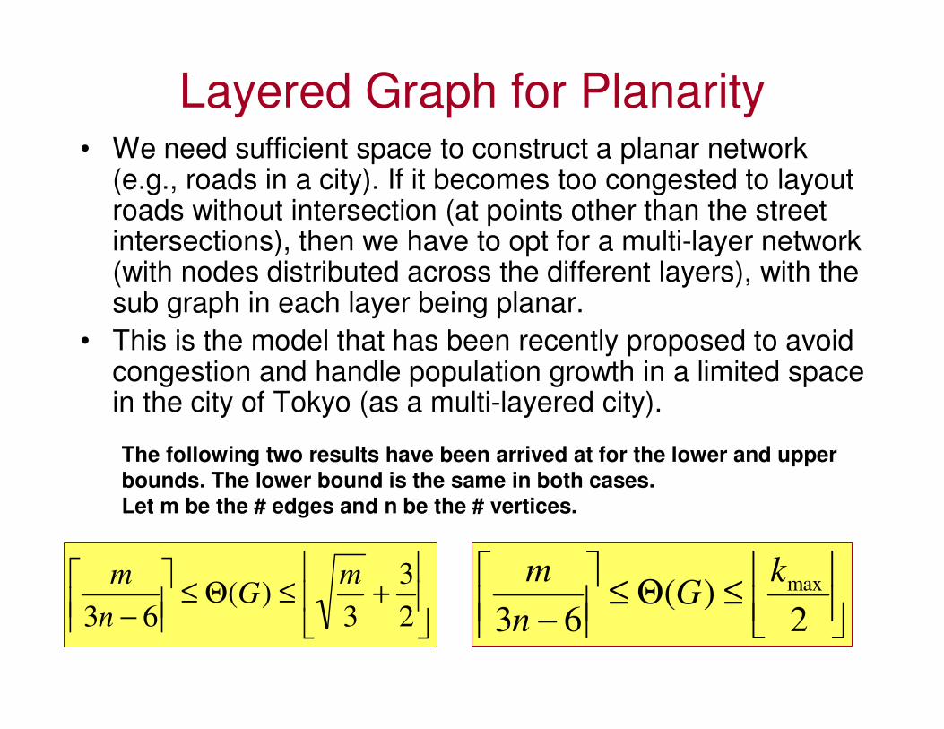
Layered Graph for Planarity• We need sufficient space to construct a planar network
(e.g., roads in a city). If it becomes too congested to layout roads without intersection (at points other than the street intersections), then we have to opt for a multi-layer network (with nodes distributed across the different layers), with the sub graph in each layer being planar.
• This is the model that has been recently proposed to avoid congestion and handle population growth in a limited space in the city of Tokyo (as a multi-layered city).
The following two results have been arrived at for the lower and upper
bounds. The lower bound is the same in both cases.
Let m be the # edges and n be the # vertices.
+≤Θ≤
− 2
3
3)(
63
mG
n
m
≤Θ≤
− 2)(
63
maxkG
n
m
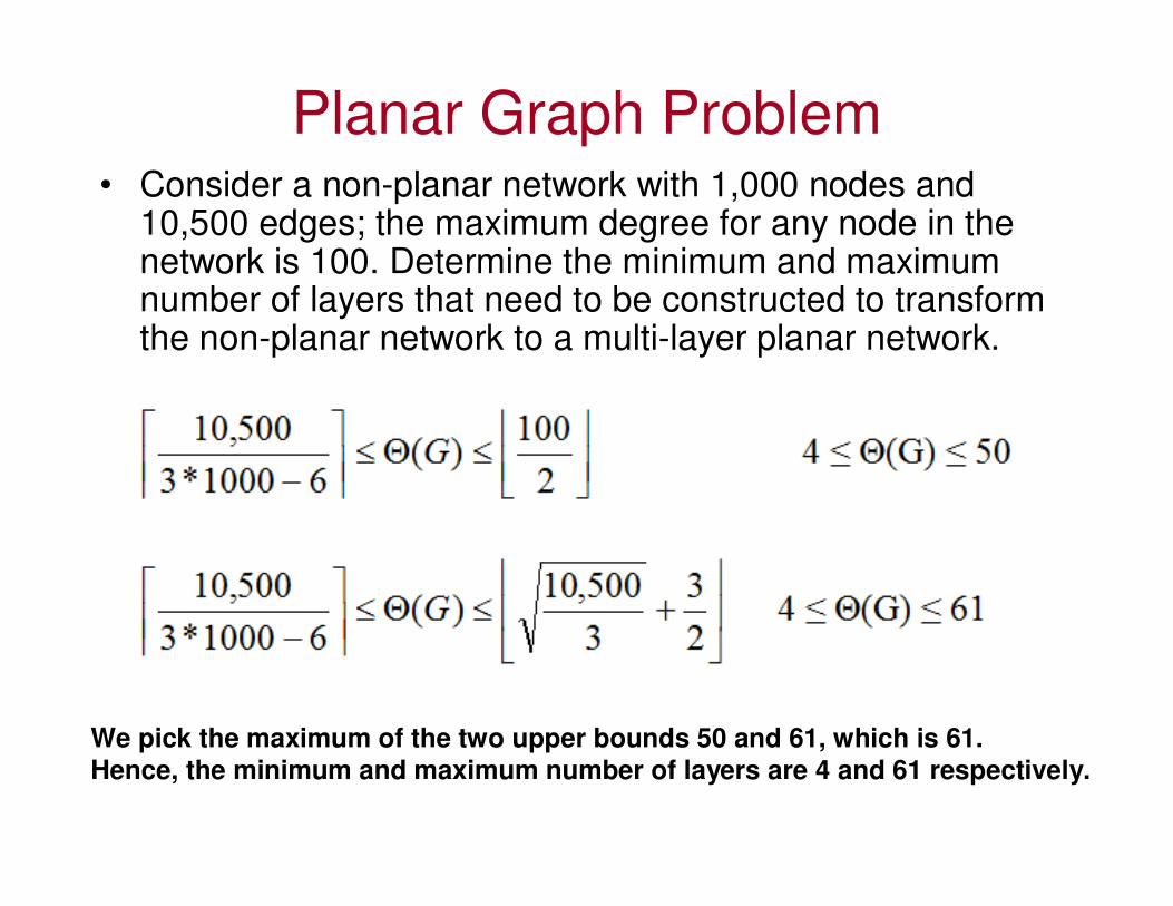
Planar Graph Problem• Consider a non-planar network with 1,000 nodes and
10,500 edges; the maximum degree for any node in the network is 100. Determine the minimum and maximum number of layers that need to be constructed to transform the non-planar network to a multi-layer planar network.
We pick the maximum of the two upper bounds 50 and 61, which is 61.Hence, the minimum and maximum number of layers are 4 and 61 respectively.
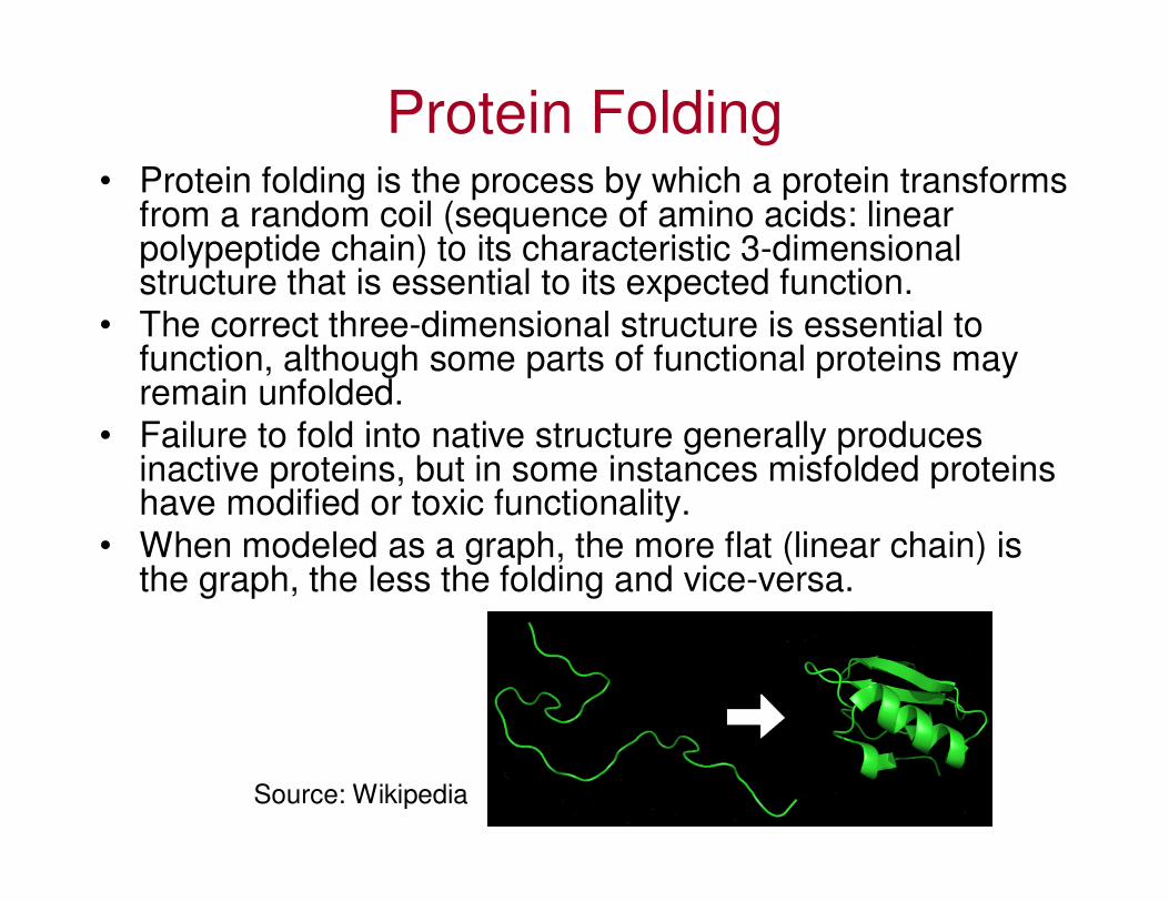
Protein Folding• Protein folding is the process by which a protein transforms
from a random coil (sequence of amino acids: linear polypeptide chain) to its characteristic 3-dimensional structure that is essential to its expected function.
• The correct three-dimensional structure is essential to function, although some parts of functional proteins may remain unfolded.
• Failure to fold into native structure generally produces inactive proteins, but in some instances misfolded proteins have modified or toxic functionality.
• When modeled as a graph, the more flat (linear chain) is the graph, the less the folding and vice-versa.
Source: Wikipedia
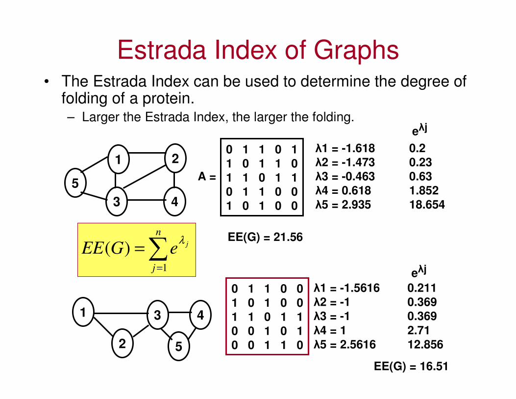
Estrada Index of Graphs• The Estrada Index can be used to determine the degree of
folding of a protein.– Larger the Estrada Index, the larger the folding.
1 2
3 4
5
0 1 1 0 1
1 0 1 1 0
1 1 0 1 1
0 1 1 0 0
1 0 1 0 0
A =
∑=
=n
j
jeGEE1
)(λ
λ1 = -1.618 0.2
λ2 = -1.473 0.23λ3 = -0.463 0.63
λ4 = 0.618 1.852
λ5 = 2.935 18.654
eλj
EE(G) = 21.56
1
2
3 4
5
0 1 1 0 0
1 0 1 0 0
1 1 0 1 10 0 1 0 10 0 1 1 0
λ1 = -1.5616 0.211
λ2 = -1 0.369
λ3 = -1 0.369
λ4 = 1 2.71λ5 = 2.5616 12.856
eλj
EE(G) = 16.51
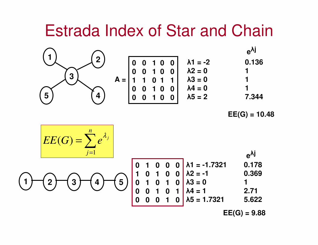
Estrada Index of Star and Chain
1 2
3
45
0 0 1 0 0
0 0 1 0 0
1 1 0 1 1
0 0 1 0 0
0 0 1 0 0
A =
∑=
=n
j
jeGEE1
)(λ
λ1 = -2 0.136
λ2 = 0 1
λ3 = 0 1
λ4 = 0 1
λ5 = 2 7.344
eλj
EE(G) = 10.48
1 2 3 4 5
0 1 0 0 0
1 0 1 0 0
0 1 0 1 0
0 0 1 0 1
0 0 0 1 0
λ1 = -1.7321 0.178
λ2 = -1 0.369
λ3 = 0 1
λ4 = 1 2.71
λ5 = 1.7321 5.622
eλj
EE(G) = 9.88

Network Returnability• By computing Estrada Index on directed networks, we can
determine how much of the information departing from a node in the network returns to it.
• Estrada Index is the weighted sum of the number of walks
of lengths k that start and end at each of the nodes in the
network.
– k = 0 corresponds to the nodes themselves and hence should be
subtracted from the sum below to determine an accurate value of
the Estrada Index for network returnability.
– In the context of network returnability, we define the Estrada Index
as: Z(D) = EE(D) – n.
Returnability Equilibrium Constant)(
)(
UZ
DZKr =
where Z(D) and Z(U) are the Estrada Index of Network Returnability values for a
directed network D and its undirected version U (with symmetric links) respy.
0 ≤ Kr ≤ 1
Kr = 0 for a directed graph
with no cycles; Kr = 1 for
a directed graph with all
bi-directional edges
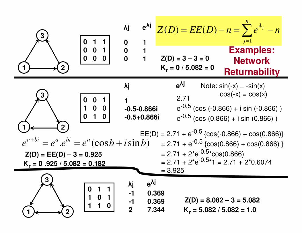
Examples: Network
Returnability1 2
30 1 1
0 0 1
0 0 0
λj
0
0
0
eλj
1
1
1
nenDEEDZn
j
j −=−= ∑=1
)()(λ
Z(D) = 3 – 3 = 0
1 2
30 0 1
1 0 0
0 1 0
λj
1
-0.5-0.866i
-0.5+0.866i
eλj
2.71
e-0.5 (cos (-0.866) + i sin (-0.866) )
e-0.5 (cos (0.866) + i sin (0.866) )
)sin(cos. bibeeeeabiabia +==+
EE(D) = 2.71 + e-0.5 {cos(-0.866) + cos(0.866)}
= 2.71 + e-0.5 {cos(0.866) + cos(0.866) }
= 2.71 + 2*e-0.5*cos(0.866)
= 2.71 + 2*e-0.5*1 = 2.71 + 2*0.6074
= 3.925
Note: sin(-x) = -sin(x)
cos(-x) = cos(x)
Z(D) = EE(D) – 3 = 0.925
1 2
3
0 1 11 0 11 1 0
λj
-1-1
2
eλj
0.3690.369
7.344
Z(D) = 8.082 – 3 = 5.082
Kr = 0 / 5.082 = 0
Kr = 0 .925 / 5.082 = 0.182
Kr = 5.082 / 5.082 = 1.0
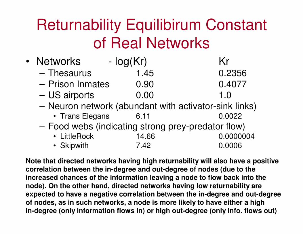
Returnability Equilibirum Constantof Real Networks
• Networks - log(Kr) Kr– Thesaurus 1.45 0.2356
– Prison Inmates 0.90 0.4077– US airports 0.00 1.0
– Neuron network (abundant with activator-sink links)• Trans Elegans 6.11 0.0022
– Food webs (indicating strong prey-predator flow)• LittleRock 14.66 0.0000004
• Skipwith 7.42 0.0006
Note that directed networks having high returnability will also have a positive
correlation between the in-degree and out-degree of nodes (due to the
increased chances of the information leaving a node to flow back into the
node). On the other hand, directed networks having low returnability are
expected to have a negative correlation between the in-degree and out-degreeof nodes, as in such networks, a node is more likely to have either a high
in-degree (only information flows in) or high out-degree (only info. flows out)
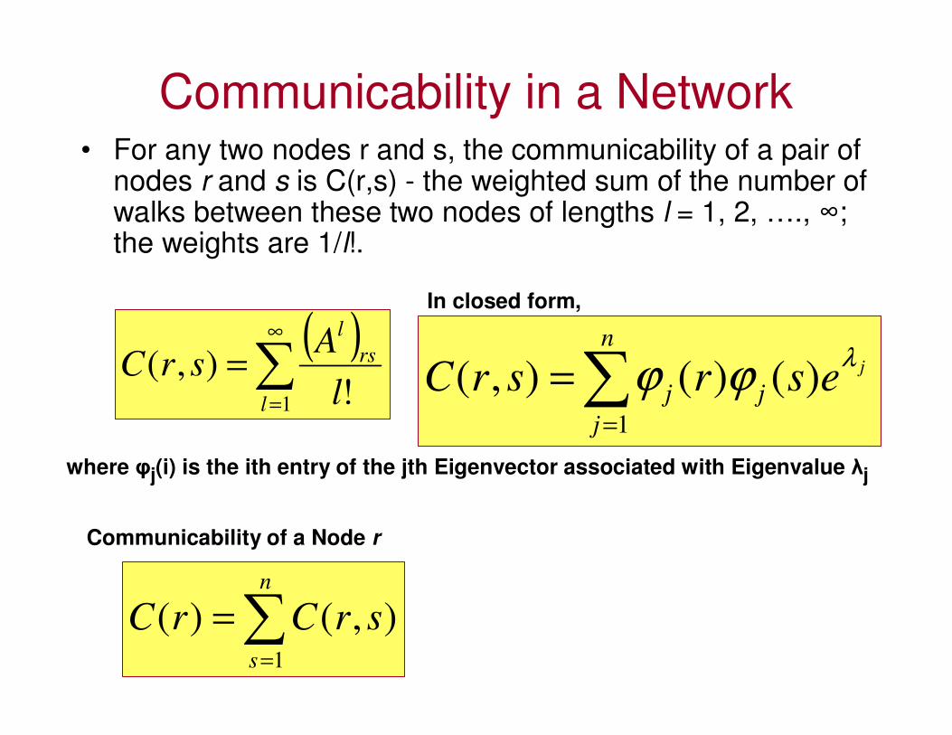
Communicability in a Network• For any two nodes r and s, the communicability of a pair of
nodes r and s is C(r,s) - the weighted sum of the number of walks between these two nodes of lengths l = 1, 2, …., ∞; the weights are 1/l!.
( )∑
∞
=
=1 !
),(l
rs
l
l
AsrC
In closed form,
∑=
=n
j
jj
jesrsrC1
)()(),(λ
ϕϕ
where φj(i) is the ith entry of the jth Eigenvector associated with Eigenvalue λj
Communicability of a Node r
∑=
=n
s
srCrC1
),()(

Example 1: Network Communicability (1)
1
2
3
4
5
6
789
10
1
2
3
4
5
6
7
8
9
10
1 2 3 4 5 6 7 8 9 10
0 1 1 1 1 0 0 0 0 0
1 0 1 1 0 1 0 0 0 0
1 1 0 1 0 0 0 1 0 0
1 1 1 0 0 0 0 0 0 0
1 0 0 0 0 1 1 0 1 1
0 1 0 0 1 0 0 0 0 0
0 0 0 0 1 0 0 1 0 0
0 0 1 0 0 0 1 0 0 0
0 0 0 0 1 0 0 0 0 0
0 0 0 0 1 0 0 0 0 0
Node IDs: 1, 2, …, 10
Eigen
Vectors

Example 1: Network Communicability (2)Even though node 5 has the highest degree
(5 links), its communicability is less than that
of the nodes in the clique (1, 2, 3, 4). The links
to peripheral nodes such as 9 and 10 does
not make any significant contributions to
the communicability of node 5. Hence, to
have high communicability, it is better for a
node to be part of a clique and/or connected
with nodes having high degree.
Each of nodes 7 and 8 have the same degree;
but, since Node 8 is connected to a node in
the clique, node 8 has high communicability.The relative
closeness of
node 6 to a high
degree node 5
helps node 2 to
gather high
communicability
compared to node 3
that is connected to node 8 which is in turn connected to a
low-degree node (node 7).
1
2
3
4
5
6
789
10
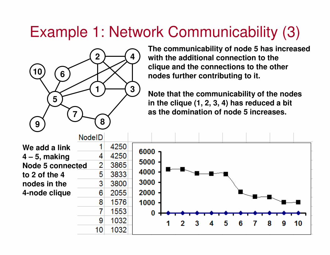
Example 1: Network Communicability (3)
1
2
3
4
5
6
789
10
The communicability of node 5 has increased
with the additional connection to the
clique and the connections to the other
nodes further contributing to it.
Note that the communicability of the nodes
in the clique (1, 2, 3, 4) has reduced a bitas the domination of node 5 increases.
We add a link
4 – 5, making
Node 5 connected
to 2 of the 4
nodes in the
4-node clique
Bipartite Graphs
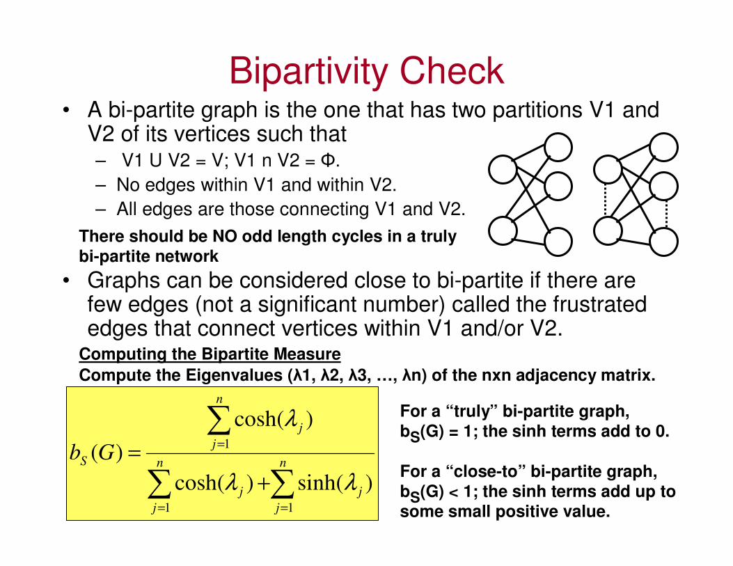
Bipartivity Check• A bi-partite graph is the one that has two partitions V1 and
V2 of its vertices such that– V1 U V2 = V; V1 n V2 = Φ.
– No edges within V1 and within V2.
– All edges are those connecting V1 and V2.
• Graphs can be considered close to bi-partite if there are few edges (not a significant number) called the frustrated edges that connect vertices within V1 and/or V2.
Computing the Bipartite Measure
Compute the Eigenvalues (λ1, λ2, λ3, …, λn) of the nxn adjacency matrix.
∑∑
∑
==
=
+
=n
j
j
n
j
j
n
j
j
S Gb
11
1
)sinh()cosh(
)cosh(
)(
λλ
λ For a “truly” bi-partite graph,
bS(G) = 1; the sinh terms add to 0.
For a “close-to” bi-partite graph,bS(G) < 1; the sinh terms add up to
some small positive value.
There should be NO odd length cycles in a truly
bi-partite network
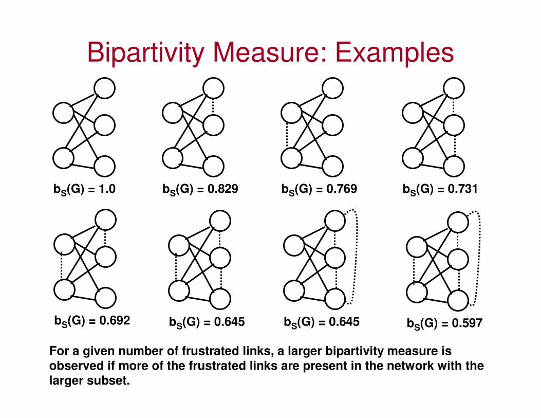
Bipartivity Measure: Examples
bS(G) = 1.0 bS(G) = 0.829 bS(G) = 0.769 bS(G) = 0.731
bS(G) = 0.692 bS(G) = 0.645 bS(G) = 0.645 bS(G) = 0.597
For a given number of frustrated links, a larger bipartivity measure isobserved if more of the frustrated links are present in the network with the
larger subset.
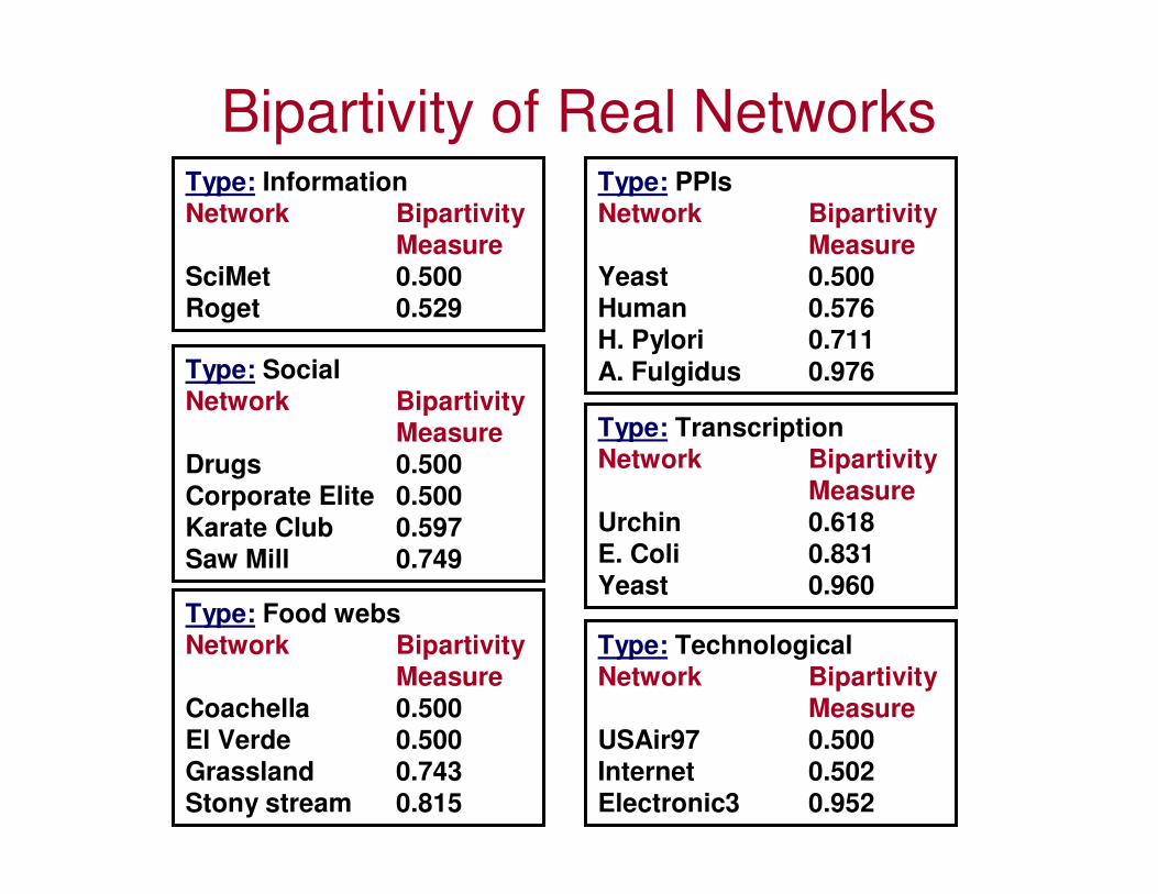
Bipartivity of Real NetworksType: Information
Network Bipartivity
MeasureSciMet 0.500
Roget 0.529
Type: Social
Network Bipartivity
Measure
Drugs 0.500
Corporate Elite 0.500
Karate Club 0.597
Saw Mill 0.749
Type: Food webs
Network Bipartivity
Measure
Coachella 0.500
El Verde 0.500
Grassland 0.743
Stony stream 0.815
Type: PPIs
Network Bipartivity
MeasureYeast 0.500
Human 0.576
H. Pylori 0.711
A. Fulgidus 0.976
Type: Transcription
Network Bipartivity
Measure
Urchin 0.618
E. Coli 0.831
Yeast 0.960
Type: Technological
Network Bipartivity
Measure
USAir97 0.500
Internet 0.502
Electronic3 0.952
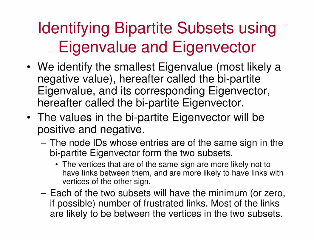
Identifying Bipartite Subsets using Eigenvalue and Eigenvector
• We identify the smallest Eigenvalue (most likely a negative value), hereafter called the bi-partite Eigenvalue, and its corresponding Eigenvector, hereafter called the bi-partite Eigenvector.
• The values in the bi-partite Eigenvector will be positive and negative.– The node IDs whose entries are of the same sign in the
bi-partite Eigenvector form the two subsets.• The vertices that are of the same sign are more likely not to
have links between them, and are more likely to have links with vertices of the other sign.
– Each of the two subsets will have the minimum (or zero, if possible) number of frustrated links. Most of the links are likely to be between the vertices in the two subsets.
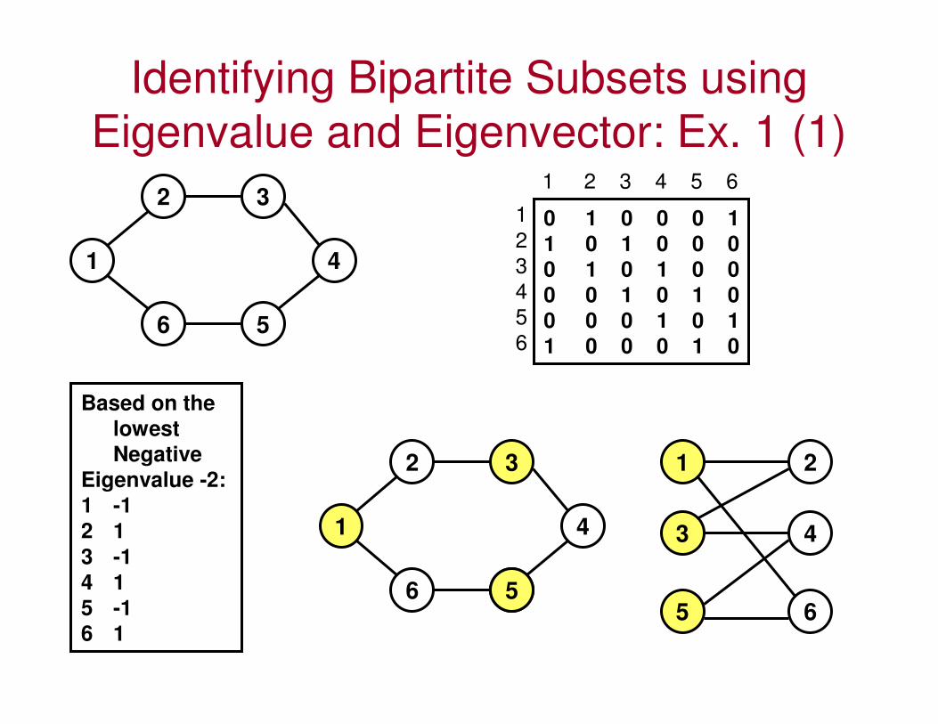
Identifying Bipartite Subsets using
Eigenvalue and Eigenvector: Ex. 1 (1)
2
1
3
4
56
1
2
3
4
5
6
1 2 3 4 5 6
0 1 0 0 0 1
1 0 1 0 0 0
0 1 0 1 0 0
0 0 1 0 1 0
0 0 0 1 0 1
1 0 0 0 1 0
Based on the
lowest
Negative
Eigenvalue -2:
1 -1
2 1
3 -1
4 1
5 -1 6 1
2
1
3
4
56
1
3
55
2
4
6

Identifying Bipartite Subsets using
Eigenvalue and Eigenvector: Ex. 1 (2)
Eigenvalue, λ cosh(λ) sinh(λ)
-2 3.7622 -3.6269
-1 1.5431 -1.1752
-1 1.5431 -1.1752
1 1.5431 1.1752
1 1.5431 1.1752
2 3.7622 -3.6269
-----------------------------------------------------------
Total 13.6968 0
∑∑
∑
==
=
+
=n
j
j
n
j
j
n
j
j
S Gb
11
1
)sinh()cosh(
)cosh(
)(
λλ
λ
13.6968
bS(G) = --------------------------
(13.6968 + 0)
= 1.0
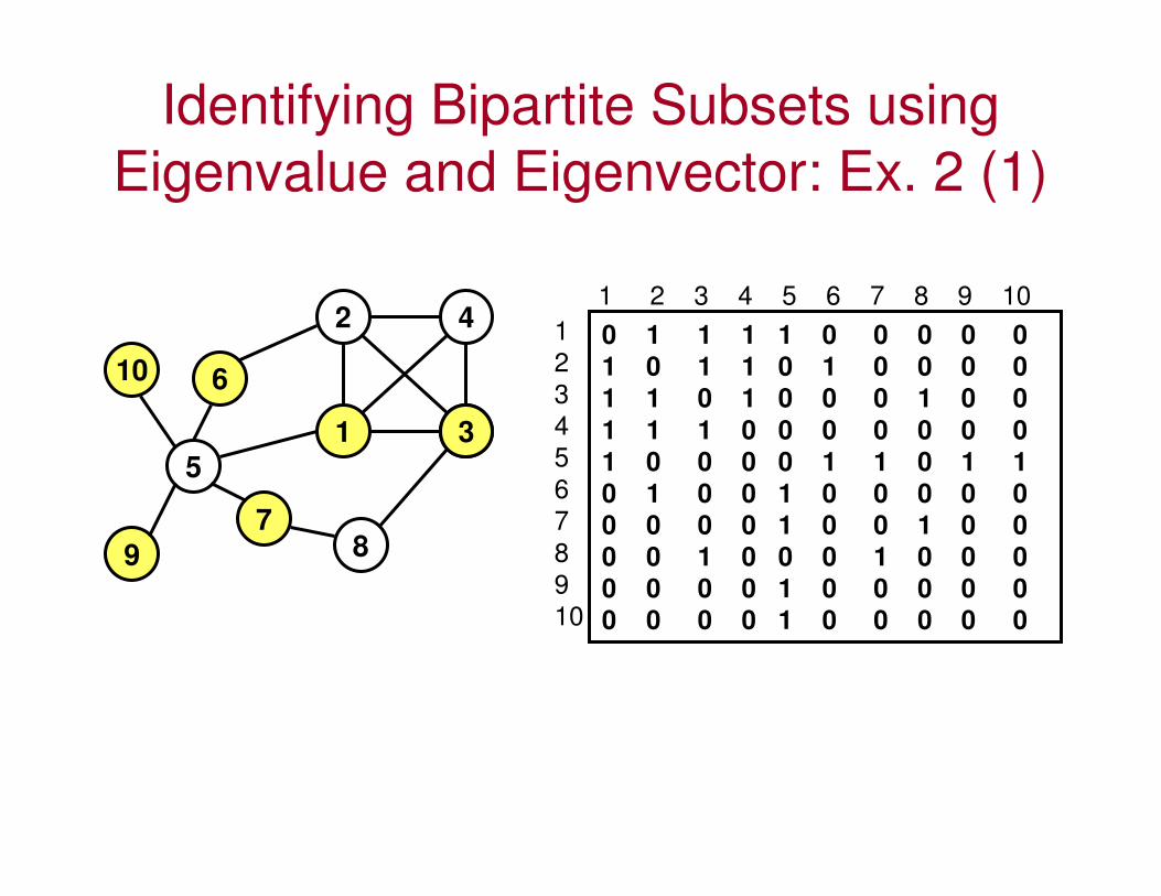
Identifying Bipartite Subsets using
Eigenvalue and Eigenvector: Ex. 2 (1)
1
2
3
4
5
6
789
10
3
1
2
3
4
5
6
7
8
9
10
1 2 3 4 5 6 7 8 9 10
0 1 1 1 1 0 0 0 0 0
1 0 1 1 0 1 0 0 0 0
1 1 0 1 0 0 0 1 0 0
1 1 1 0 0 0 0 0 0 0
1 0 0 0 0 1 1 0 1 1
0 1 0 0 1 0 0 0 0 0
0 0 0 0 1 0 0 1 0 0
0 0 1 0 0 0 1 0 0 0
0 0 0 0 1 0 0 0 0 0
0 0 0 0 1 0 0 0 0 0
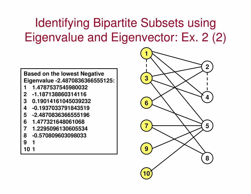
Identifying Bipartite Subsets using
Eigenvalue and Eigenvector: Ex. 2 (2)
Based on the lowest Negative
Eigenvalue -2.4870836366555125:
1 1.4787537545980032
2 -1.187138860314116
3 0.19014161045039232
4 -0.1937033791843519
5 -2.4870836366555196
6 1.477321648061068
7 1.2295096130605534
8 -0.570809603098033
9 1
10 1
1
3
6
7
9
10
2
4
5
8

Identifying Bipartite Subsets using
Eigenvalue and Eigenvector: Ex. 2 (3)
Eigenvalue, λ cosh(λ) sinh(λ)
-2.4871 6.0547 -5.9716
1.6828 2.7832 -2.5974
-1.3098 1.9877 -1.7178
-0.8564 1.3897 -0.9650
-0.3741 1.0708 -0.3829
0 1.0 0
0.3197 1.0515 0.3252
1.1131 1.6862 1.3576
1.8880 3.3788 3.2274
3.3893 14.839 14.8057
-----------------------------------------------------------
Total 35.2416 8.0812
∑∑
∑
==
=
+
=n
j
j
n
j
j
n
j
j
S Gb
11
1
)sinh()cosh(
)cosh(
)(
λλ
λ
35.2416
bS(G) = --------------------------
(35.2416 + 8.0812)
= 0.8135
Bipartite Partition Detection: Digraph
• When confronted with a directed graph, first transform the directed graph to an undirected graph and determine the two partitions as
explained previously using the Eigenvector approach.
• After identifying the partitions, restore the directions of the edges.
• In a directed graph, the edges typically point from one set of vertices to the other set of vertices.
– There could be scenarios where the edges could point
in the reverse direction; as long as we know the
direction of the edges, we could restore them after determining the two partitions.
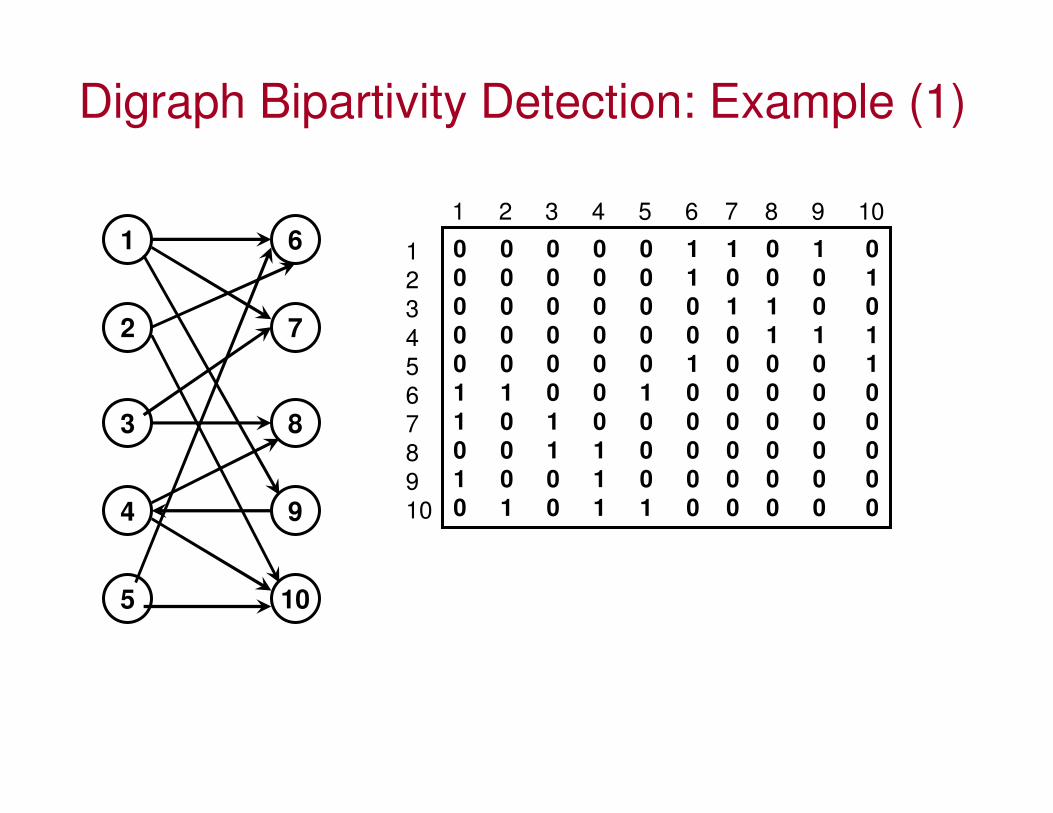
Digraph Bipartivity Detection: Example (1)
1
2
3
4
5
6
7
8
9
10
1
2
3
4
5
6
7
8
9
10
1 2 3 4 5 6 7 8 9 10
0 0 0 0 0 1 1 0 1 0
0 0 0 0 0 1 0 0 0 1
0 0 0 0 0 0 1 1 0 0
0 0 0 0 0 0 0 1 1 1
0 0 0 0 0 1 0 0 0 1
1 1 0 0 1 0 0 0 0 0
1 0 1 0 0 0 0 0 0 0
0 0 1 1 0 0 0 0 0 0
1 0 0 1 0 0 0 0 0 0
0 1 0 1 1 0 0 0 0 0
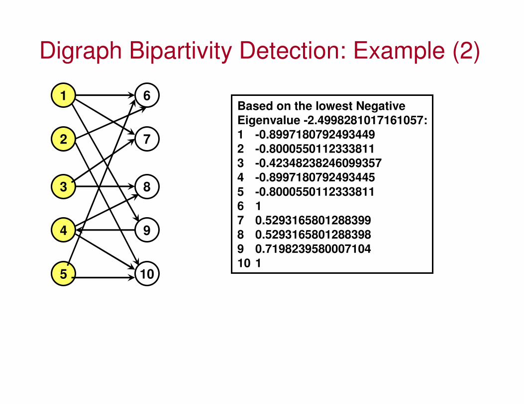
Digraph Bipartivity Detection: Example (2)
1
2
3
4
5
6
7
8
9
10
Based on the lowest Negative
Eigenvalue -2.4998281017161057:
1 -0.8997180792493449
2 -0.8000550112333811
3 -0.42348238246099357
4 -0.8997180792493445
5 -0.8000550112333811
6 1
7 0.5293165801288399
8 0.5293165801288398
9 0.7198239580007104
10 1