Embed Size (px)
Citation preview

Graph Regularized Nonnegative MatrixFactorization for Data Representation
Deng Cai, Member, IEEE, Xiaofei He, Senior Member, IEEE,
Jiawei Han, Fellow, IEEE, and Thomas S. Huang, Fellow, IEEE
Abstract—Matrix factorization techniques have been frequently applied in information retrieval, computer vision, and pattern
recognition. Among them, Nonnegative Matrix Factorization (NMF) has received considerable attention due to its psychological and
physiological interpretation of naturally occurring data whose representation may be parts based in the human brain. On the other
hand, from the geometric perspective, the data is usually sampled from a low-dimensional manifold embedded in a high-dimensional
ambient space. One then hopes to find a compact representation,which uncovers the hidden semantics and simultaneously respects
the intrinsic geometric structure. In this paper, we propose a novel algorithm, called Graph Regularized Nonnegative Matrix
Factorization (GNMF), for this purpose. In GNMF, an affinity graph is constructed to encode the geometrical information and we seek a
matrix factorization, which respects the graph structure. Our empirical study shows encouraging results of the proposed algorithm in
comparison to the state-of-the-art algorithms on real-world problems.
Index Terms—Nonnegative matrix factorization, graph Laplacian, manifold regularization, clustering.
Ç
1 INTRODUCTION
THE techniques for matrix factorization have becomepopular in recent years for data representation. In many
problems in information retrieval, computer vision, andpattern recognition, the input data matrix is of very highdimension. This makes learning from example infeasible [15].One then hopes to find two or more lower dimensionalmatrices whose product provides a good approximation tothe original one. The canonical matrix factorization techni-ques include LU decomposition, QR decomposition, vectorquantization, and Singular Value Decomposition (SVD).
SVD is one of the most frequently used matrix factoriza-
tion techniques. A singular value decomposition of an M �N matrix X has the following form:
X ¼ U�VT ;
where U is an M �M orthogonal matrix, V is an N �Northogonal matrix, and � is an M �N diagonal matrix with
�ij ¼ 0 if i 6¼ j and �ii � 0. The quantities �ii are called the
singular values of X, and the columns of U and V are called
left and right singular vectors, respectively. By removingthose singular vectors corresponding to sufficiently smallsingular values, we get a low-rank approximation to theoriginal matrix. This approximation is optimal in terms ofthe reconstruction error, and thus optimal for datarepresentation when euclidean structure is concerned. Forthis reason, SVD has been applied to various real-worldapplications such as face recognition (eigenface, [40]) anddocument representation (latent semantic indexing, [11]).
Previous studies have shown that there is psychologicaland physiological evidence for parts-based representationin the human brain [34], [41], [31]. The Nonnegative MatrixFactorization (NMF) algorithm is proposed to learn theparts of objects like human faces and text documents [33],[26]. NMF aims to find two nonnegative matrices whoseproduct provides a good approximation to the originalmatrix. The nonnegative constraints lead to a parts-basedrepresentation because they allow only additive, notsubtractive, combinations. NMF has been shown to besuperior to SVD in face recognition [29] and documentclustering [42]. It is optimal for learning the parts of objects.
Recently, various researchers (see [39], [35], [1], [36], [2])have considered the case when the data is drawn fromsampling a probability distribution that has support on ornear to a submanifold of the ambient space. Here, ad-dimensional submanifold of a euclidean space IRM is asubset Md � IRM , which locally looks like a flat d-dimen-sional euclidean space [28]. In order to detect the under-lying manifold structure, many manifold learning algorithmshave been proposed, such as Locally Linear Embedding(LLE) [35], ISOMAP [39], and Laplacian Eigenmap [1]. Allof these algorithms use the so-called locally invariant idea[18], i.e., the nearby points are likely to have similarembeddings. It has been shown that learning performancecan be significantly enhanced if the geometrical structure isexploited and the local invariance is considered.
1548 IEEE TRANSACTIONS ON PATTERN ANALYSIS AND MACHINE INTELLIGENCE, VOL. 33, NO. 8, AUGUST 2011
. D. Cai and X. He are with the State Key Lab of CAD&CG, College ofComputer Science, Zhejiang University, 388 Yu Hang Tang Rd.,Hangzhou, Zhejiang 310058, China.E-mail: {dengcai, xiaofeihe}@cad.zju.edu.cn.
. J. Han is with the Department of Computer Science, University of Illinoisat Urbana Champaign, Siebel Center, 201 N. Goodwin Ave., Urbana, IL61801. E-mail: [email protected].
. T.S. Huang is with the Beckman Institute for Advanced Sciences andTechnology, University of Illinois at Urbana Champaign, BeckmanInstitute Center, 405 North Mathews Ave., Urbana, IL 61801.E-mail: [email protected].
Manuscript received 28 Apr. 2009; revised 21 Dec. 2009; accepted 22 Oct.2010; published online 13 Dec. 2010.Recommended for acceptance by D.D. Lee.For information on obtaining reprints of this article, please send e-mail to:[email protected], and reference IEEECS Log NumberTPAMI-2009-04-0266.Digital Object Identifier no. 10.1109/TPAMI.2010.231.
0162-8828/11/$26.00 � 2011 IEEE Published by the IEEE Computer Society

Motivated by recent progress in matrix factorization andmanifold learning [2], [5], [6], [7], in this paper we propose anovel algorithm, called Graph regularized NonnegativeMatrix Factorization (GNMF), which explicitly considersthe local invariance. We encode the geometrical informationof the data space by constructing a nearest neighbor graph.Our goal is to find a parts-based representation space inwhich two data points are sufficiently close to each other, ifthey are connected in the graph. To achieve this, we designa new matrix factorization objective function and incorpo-rate the graph structure into it. We also develop anoptimization scheme to solve the objective function basedon iterative updates of the two factor matrices. This leads toa new parts-based data representation which respects thegeometrical structure of the data space. The convergenceproof of our optimization scheme is provided.
It is worthwhile to highlight several aspects of the
proposed approach here:
1. While the standard NMF fits the data in a euclideanspace, our algorithm exploits the intrinsic geometryof the data distribution and incorporates it as anadditional regularization term. Hence, our algorithmis particularly applicable when the data are sampledfrom a submanifold which is embedded in high-dimensional ambient space.
2. Our algorithm constructs a nearest neighbor graphto model the manifold structure. The weight matrixof the graph is highly sparse. Therefore, the multi-plicative update rules for GNMF are very efficient.By preserving the graph structure, our algorithm canhave more discriminating power than the standardNMF algorithm.
3. Recent studies [17], [13] show that NMF is closelyrelated to Probabilistic Latent Semantic Analysis(PLSA) [21]. The latter is one of the most populartopic modeling algorithms. Specifically, NMF withKL-divergence formulation is equivalent to PLSA[13]. From this viewpoint, the proposed GNMFapproach also provides a principled way for incorpor-ating the geometrical structure into topic modeling.
4. The proposed framework is a general one that canleverage the power of both NMF and graph Laplacianregularization. Besides the nearest neighbor informa-tion, other knowledge (e.g., label information, socialnetwork structure) about the data can also be used toconstruct the graph. This naturally leads to otherextensions (e.g., semi-supervised NMF).
The rest of the paper is organized as follows: In Section 2,we give a brief review of NMF. Section 3 introduces ouralgorithm and provides a convergence proof of ouroptimization scheme. Extensive experimental results onclustering are presented in Section 4. Finally, we providesome concluding remarks and suggestions for future workin Section 5.
2 A BRIEF REVIEW OF NMF
NMF [26] is a matrix factorization algorithm that focuses
on the analysis of data matrices whose elements are
nonnegative.
Given a data matrix X ¼ ½x1; . . . ;xN � 2 IRM�N , eachcolumn of X is a sample vector. NMF aims to find twononnegative matrices U ¼ ½uik� 2 IRM�K and V ¼ ½vjk� 2IRN�K whose product can well approximate the originalmatrix X:
X � UVT :
There are two commonly used cost functions that quantifythe quality of the approximation. The first one is the square ofthe euclidean distance between two matrices (the square ofthe Frobenius norm of two matrices difference) [33]:
O1 ¼ kX�UVTk2 ¼Xi;j
xij �XKk¼1
uikvjk
!2
: ð1Þ
The second one is the “divergence” between twomatrices [27]:
O2 ¼ DðXkUVT Þ ¼Xi;j
xij logxijyij� xij þ yij
� �; ð2Þ
where Y ¼ ½yij� ¼ UVT . This cost function is referred to as“divergence” of X from Y instead of “distance” between Xand Y because it is not symmetric. In other words,DðXkYÞ 6¼ DðYkXÞ. It reduces to the Kullback-Leiblerdivergence or relative entropy, when
Pij xij ¼
Pij yij ¼ 1,
so that X and Y can be regarded as normalized probabilitydistributions. We will refer O1 as F-norm formulation andO2 as divergence formulation in the rest of the paper.
Although the objective functions O1 in (1) and O2 in (2)are convex in U only or V only, they are not convex in bothvariables together. Therefore, it is unrealistic to expect analgorithm to find the global minimum of O1 (or O2). Leeand Seung [27] presented two iterative update algorithms.The algorithm minimizing the objective function O1 in (1) isas follows:
uik uikðXVÞikðUVTVÞik
; vjk vjkðXTUÞjkðVUTUÞjk
:
The algorithm minimizing the objective function O2 in (2) is
uik uik
Pj xijvjk=
Pk uikvjk
� �P
j vjk;
vjk vjk
Pi xijuik=
Pk uikvjk
� �Pi uik
:
It is proven that the above two algorithms will find localminima of the objective functions O1 and O2 [27].
In reality, we have K �M and K � N . Thus, NMFessentially tries to find a compressed approximation of theoriginal data matrix. We can view this approximationcolumn by column as
xj �XKk¼1
ukvjk; ð3Þ
where uk is the kth column vector of U. Thus, each datavector xj is approximated by a linear combination of thecolumns of U, weighted by the components of V. Therefore,U can be regarded as containing a basis, that is, optimized
CAI ET AL.: GRAPH REGULARIZED NONNEGATIVE MATRIX FACTORIZATION FOR DATA REPRESENTATION 1549

for the linear approximation of the data in X. Let zTj denotethe jth row of V, zj ¼ ½vj1; . . . ; vjk�T . zj can be regarded as thenew representation of the jth data point with respect to thenew basis U. Since relatively few basis vectors are used torepresent many data vectors, a good approximation can onlybe achieved if the basis vectors discover structure that islatent in the data [27].
The nonnegative constraints on U and V only allowadditive combinations among different bases. This is themost significant difference between NMF and the othermatrix factorization methods, e.g., SVD. Unlike SVD, nosubtractions can occur in NMF. For this reason, it isbelieved that NMF can learn a parts-based representation[26]. The advantages of this parts-based representation havebeen observed in many real-world problems such as faceanalysis [29], document clustering [42], and DNA geneexpression analysis [3].
3 GRAPH REGULARIZED NONNEGATIVE MATRIX
FACTORIZATION
By using the nonnegative constraints, NMF can learn aparts-based representation. However, NMF performs thislearning in the euclidean space. It fails to discover theintrinsic geometrical and discriminating structure of thedata space, which is essential to the real-world applications.In this section, we introduce our GNMF algorithm, whichavoids this limitation by incorporating a geometricallybased regularizer.
3.1 NMF with Manifold Regularization
Recall that NMF tries to find a set of basis vectors that canbe used to best approximate the data. One might furtherhope that the basis vectors can respect the intrinsicRiemannian structure, rather than ambient euclideanstructure. A natural assumption here could be that if twodata points xj;xl are close in the intrinsic geometry of thedata distribution, then zj and zl, the representations of thesetwo points with respect to the new basis, are also close toeach other. This assumption is usually referred to as localinvariance assumption [1], [19], [7], which plays an essentialrole in the development of various kinds of algorithms,including dimensionality reduction algorithms [1] andsemi-supervised learning algorithms [2], [46], [45].
Recent studies in spectral graph theory [9] and manifoldlearning theory [1] have demonstrated that the localgeometric structure can be effectively modeled through anearest neighbor graph on a scatter of data points. Considera graph with N vertices, where each vertex corresponds to adata point. For each data point xj, we find its p nearestneighbors and put edges between xj and its neighbors.There are many choices to define the weight matrix W onthe graph. Three of the most commonly used are as follows:
1. 0-1 Weighting. Wjl ¼ 1, if and only if nodes j and lare connected by an edge. This is the simplestweighting method and is very easy to compute.
2. Heat Kernel Weighting. If nodes j and l areconnected, put
Wjl ¼ e�kxj�xlk2
� :
Heat kernel has an intrinsic connection to theLaplace-Beltrami operator on differentiable func-tions on a manifold [1].
3. Dot-Product Weighting. If nodes j and l areconnected, put
Wjl ¼ xTj xl:
Note that if x is normalized to 1, the dot product oftwo vectors is equivalent to the cosine similarity ofthe two vectors.
The Wjl is used to measure the closeness of two points xjand xl. The different similarity measures are suitable fordifferent situations. For example, the cosine similarity (dot-product weighting) is very popular in the IR community(for processing documents), while for image data, the heatkernel weight may be a better choice. Since Wjl in our paperis only for measuring the closeness, we do not treat thedifferent weighting schemes separately.
The low-dimensional representation of xj with respect tothe new basis is zj ¼ ½vj1; . . . ; vjk�T . Again, we can use eithereuclidean distance
dðzj; zlÞ ¼ kzj � zlk2;
or divergence
DðzjkzlÞ ¼XKk¼1
vjk logvjkvlk� vjk þ vlk
� �;
to measure the “dissimilarity” between the low-dimen-sional representations of two data points with respect to thenew basis.
With the above defined weight matrix W, we can use thefollowing two terms to measure the smoothness of the low-dimensional representation
R2 ¼1
2
XNj;l¼1
ðDðzjkzlÞ þDðzlkzjÞÞWjl
¼ 1
2
XNj;l¼1
XKk¼1
vjk logvjkvlkþ vlk log
vlkvjk
� �Wjl;
ð4Þ
and
R1 ¼1
2
XNj;l¼1
kzj � zlk2Wjl
¼XNj¼1
zTj zjDjj �XNj;l¼1
zTj zlWjl
¼ TrðVTDVÞ � TrðVTWVÞ ¼ TrðVTLVÞ;
ð5Þ
where TrðÞ denotes the trace of a matrix and D is adiagonal matrix whose entries are column (or row, since Wis symmetric) sums of W;Djj ¼
Pl Wjl. L ¼ D�W, which
is called graph Laplacian [9].By minimizing R1 (or R2), we expect that if two data
points xj and xl are close (i.e., Wjl is big), zj and zl are alsoclose to each other. Combining this geometrically-basedregularizer with the original NMF objective function leadsto our GNMF.
Given a data matrix X ¼ ½xij� 2 IRM�N , our GNMF aimsto find two nonnegative matrices U ¼ ½uik� 2 IRM�K and
1550 IEEE TRANSACTIONS ON PATTERN ANALYSIS AND MACHINE INTELLIGENCE, VOL. 33, NO. 8, AUGUST 2011

V ¼ ½vjk� 2 IRN�K . Similarly to NMF, we can also use two“distance” measures here. If the euclidean distance is used,GNMF minimizes the objective function as follows:
O1 ¼ kX�UVTk2 þ �TrðVTLVÞ: ð6Þ
If the divergence is used, GNMF minimizes
O2 ¼XMi¼1
XNj¼1
xij logxijPK
k¼1 uikvjk� xij þ
XKk¼1
uikvjk
!
þ �2
XNj¼1
XNl¼1
XKk¼1
vjk logvjkvlkþ vlk log
vlkvjk
� �Wjl;
ð7Þ
where the regularization parameter � � 0 controls thesmoothness of the new representation.
3.2 Updating Rules Minimizing (6)
The objective functions O1 and O2 of GNMF in (6) and (7)are not convex in both U and V together. Therefore, it isunrealistic to expect an algorithm to find the global minima.In the following, we introduce two iterative algorithmswhich can achieve local minima.
We first discuss how to minimize the objective functionO1,which can be rewritten as
O1 ¼ Tr�ðX�UVT ÞðX�UVT ÞT
�þ �TrðVTLVÞ
¼ Tr�XXT
�� 2Tr
�XVUT
�þ Tr
�UVTVUT
�þ �TrðVTLVÞ;
ð8Þ
where the second equality applies the matrix propertiesTrðABÞ ¼ TrðBAÞ and TrðAÞ ¼ TrðAT Þ. Let ik and �jk bethe lagrange multiplier for constraint uik � 0 and vjk � 0,respectively, and � ¼ ½ ik�, � ¼ ½�jk�, the Lagrange L is
L ¼ Tr�XXT
�� 2Tr
�XVUT
�þ Tr
�UVTVUT
�þ �TrðVTLVÞ þ Trð�UT Þ þ Trð�VT Þ:
ð9Þ
The partial derivatives of L with respect to U and V are
@L@U¼ �2XVþ 2UVTVþ�; ð10Þ
@L@V¼ �2XTUþ 2VUTUþ 2�LVþ �: ð11Þ
Using the KKT conditions ikuik ¼ 0 and �jkvjk ¼ 0, we getthe following equations for uik and vjk:
� ðXVÞikuik þ ðUVTVÞikuik ¼ 0; ð12Þ
� ðXTUÞjkvjk þ ðVUTUÞjkvjk þ �ðLVÞjkvjk ¼ 0: ð13Þ
These equations lead to the following updating rules:
uik uikðXVÞikðUVTVÞik
; ð14Þ
vjk vjkðXTUþ �WVÞjkðVUTUþ �DVÞjk
: ð15Þ
Regarding these two updating rules, we have thefollowing theorem:
Theorem 1. The objective function O1 in (6) is nonincreasingunder the updating rules in (14) and (15).
Please see the Appendix for a detailed proof for theabove theorem. Our proof essentially follows the idea in theproof of Lee and Seung’s [27] paper for the original NMF.Recent studies [8], [30] show that Lee and Seung’s [27]multiplicative algorithm cannot guarantee the convergenceto a stationary point. Particularly, Lin [30] suggests minormodifications on Lee and Seung’s algorithm, which canconverge. Our updating rules in (14) and (15) are essentiallysimilar to the updating rules for NMF, and therefore, Lin’smodifications can also be applied.
When � ¼ 0, it is easy to check that the updating rules in(14) and (15) reduce to the updating rules of the original NMF.
For the objective function of NMF, it is easy to checkthat if U and V are the solution, then UD;VD�1 will alsoform a solution for any positive diagonal matrix D. Toeliminate this uncertainty, in practice, people will furtherrequire that the euclidean length of each column vector inmatrix U (or V) is 1 [42]. The matrix V (or U) will beadjusted accordingly so that UVT does not change. Thiscan be achieved by
uik uikffiffiffiffiffiffiffiffiffiffiffiffiffiffiPi u
2ik
q ; vjk vjk
ffiffiffiffiffiffiffiffiffiffiffiffiffiffiXi
u2ik
r: ð16Þ
Our GNMF also adopts this strategy. After the multi-plicative updating procedure converges, we set theeuclidean length of each column vector in matrix U to 1and adjust the matrix V so that UVT does not change.
3.3 Connection to Gradient Descent Method
Another general algorithm for minimizing the objectivefunction of GNMF in (6) is gradient descent [25]. For ourproblem, gradient descent leads to the following additiveupdate rules:
uik uik þ �ik@O1
@uik; vjk vjk þ �jk
@O1
@vjk: ð17Þ
The �ik and �jk are usually referred as step size parameters.As long as �ik and �jk are sufficiently small, the aboveupdates should reduce O1 unless U and V are at astationary point.
Generally speaking, it is relatively difficult to set thesestep size parameters while still maintaining the non-negativity of uik and vjk. However, with the special form ofthe partial derivatives, we can use some tricks to set the stepsize parameters automatically. Let �ik ¼ �uik=2ðUVTVÞik,we have
uik þ �ik@O1
@uik¼ uik �
uik
2ðUVTVÞik@O1
@uik
¼ uik �uik
2ðUVTVÞikð�2ðXVÞik þ 2ðUVTVÞikÞ
¼ uikðXVÞikðUVTVÞik
:
ð18Þ
CAI ET AL.: GRAPH REGULARIZED NONNEGATIVE MATRIX FACTORIZATION FOR DATA REPRESENTATION 1551

Similarly, letting �jk ¼ �vjk=2ðVUTUþ �DVÞjk, we have
vjk þ �jk@O1
@vjk¼ vjk �
vjk
2ðVUTUþ �DVÞjk@O1
@vjk
¼ vjk �vjk
2ðVUTUþ �DVÞjkð�2ðXTUÞjk
þ 2ðVUTUÞjk þ 2�ðLVÞjkÞ
¼ vjkðXTUþ �WVÞjkðVUTUþ �DVÞjk
:
ð19Þ
Now, it is clear that the multiplicative updating rules in (14)and (15) are special cases of gradient descent with anautomatic step parameter selection. The advantage ofmultiplicative updating rules is the guarantee of nonnega-tivity of U and V. Theorem 1 also guarantees that themultiplicative updating rules in (14) and (15) converge to alocal optimum.
3.4 Updating Rules Minimizing (7)
For the divergence formulation of GNMF, we also have twoupdating rules, which can achieve a local minimum of (7):
uik uik
Pj xijvjk=
Pk uikvjk
� �P
j vjk; ð20Þ
vk Xi
uikIþ �L
!�1v1k
Pi xi1uik=
Pk uikv1k
� �v2k
Pi xi2uik=
Pk uikv2k
� �...
vNkP
i xiNuik=P
k uikvNk� �
26664
37775;
ð21Þ
where vk is the kth column of V and I is an N �N identitymatrix.
Similarly, we have the following theorem:
Theorem 2. The objective function O2 in (7) is nonincreasing
with the updating rules in (20) and (21). The objective
function is invariant under these updates if and only if U and
V are at a stationary point.
Please see the Appendix for a detailed proof. Theupdating rules in this section (minimizing the divergenceformulation of (7)) are different from the updating rules inSection 3.2 (minimizing the F-norm formulation). For the
divergence formulation of NMF, previous studies [16]successfully analyzed the convergence property of themultiplicative algorithm [27] from EM algorithm’s max-imum likelihood point of view. Such an analysis is alsovalid in the GNMF case.
When � ¼ 0, it is easy to check that the updating rulesin (20) and (21) reduce to the updating rules of theoriginal NMF.
3.5 Computational Complexity Analysis
In this section, we discuss the extra computational cost of ourproposed algorithm in comparison to standard NMF.Specifically, we provide the computational complexityanalysis of GNMF for both the F-Norm and KL-Divergenceformulations.
The common way to express the complexity of onealgorithm is using big O notation [10]. However, this is notprecise enough to differentiate between the complexities ofGNMF and NMF. Thus, we count the arithmetic operationsfor each algorithm.
Based on the updating rules, it is not hard to count thearithmetic operations of each iteration in NMF. Wesummarize the result in Table 1. For GNMF, it is importantto note that W is a sparse matrix. If we use a p-nearestneighbor graph, the average nonzero elements on each rowof W is p. Thus, we only need NpK flam (a floating-pointaddition and multiplication) to compute WV. We alsosummarize the arithmetic operations for GNMF in Table 1.
The updating rule (21) in GNMF with the divergenceformulation involves inverting a large matrix
Pi uikIþ �L.
In reality, there is no need to actually compute the inversion.We only need to solve the linear equations system as follows:
Xi
uikIþ �L
!vk ¼
v1k
Pi xi1uik=
Pk uikv1k
� �v2k
Pi xi2uik=
Pk uikv2k
� �...
vNkP
i xiNuik=P
k uikvNk� �
2666664
3777775:
Since matrixP
i uikIþ �L is symmetric, positive definite,and sparse, we can use the iterative algorithm CG [20] tosolve this linear system of equations very efficiently. In eachiteration, CG needs to compute the matrix-vector productsin the form of ð
Pi uikIþ �LÞp. The remaining work load of
CG in each iteration is 4N flam. Thus, the time cost of CG in
1552 IEEE TRANSACTIONS ON PATTERN ANALYSIS AND MACHINE INTELLIGENCE, VOL. 33, NO. 8, AUGUST 2011
TABLE 1Computational Operation Counts for Each Iteration in NMF and GNMF
fladd: a floating-point addition, flmlt: a floating-point multiplication, fldiv: a floating-point division.N: the number of sample points, M: the number of features, K: the number of factors.p: the number of nearest neighbors, q: the number of iterations in Conjugate Gradient (CG).

each iteration is pN þ 4N . If CG stops after q iterations, thetotal time cost is qðpþ 4ÞN . CG converges very fast, usuallywithin 20 iterations. Since we need to solve K linearequations systems, the total time cost is qðpþ 4ÞNK.
Besides the multiplicative updates, GNMF also needsOðN2MÞ to construct the p-nearest neighbor graph. Suppos-ing the multiplicative updates stops after t iterations, theoverall cost for NMF (both formulations) is
OðtMNKÞ: ð22Þ
The overall cost for GNMF with F-norm formulation is
OðtMNK þN2MÞ; ð23Þ
and the cost for GNMF with divergence formulation is
OðtðM þ qðpþ 4ÞÞNK þN2MÞ: ð24Þ
4 EXPERIMENTAL RESULTS
Previous studies show that NMF is very powerful forclustering, especially in the document clustering and imageclustering tasks [42], [37]. It can achieve similar or betterperformance than most of the state-of-the-art clusteringalgorithms, including the popular spectral clusteringmethods [32], [42].
Assume that a document corpus is comprised ofK clusters each of which corresponds to a coherent topic.To accurately cluster the given document corpus, it is idealto project the documents into a K-dimensional semanticspace in which each axis corresponds to a particular topic[42]. In this semantic space, each document can berepresented as a linear combination of the K topics. Becauseit is more natural to consider each document as an additiverather than a subtractive mixture of the underlying topics,the combination coefficients should all take nonnegativevalues [42]. These values can be used to decide the clustermembership. In appearance-based visual analysis, an imagemay be also associated with some hidden parts. Forexample, a face image can be thought of as a combinationof nose, mouth, eyes, etc. It is also reasonable to require thecombination coefficients to be non-negative. This is themain motivation of applying NMF on document and imageclustering. In this section, we also evaluate our GNMFalgorithm on document and image clustering problems.
For the purpose of reproducibility, we provide the codeand data sets at: http://www.zjucadcg.cn/dengcai/GNMF/.
4.1 Data Sets
Three data sets are used in the experiment. Two of them areimage data sets and the third one is a document corpus. Theimportant statistics of these data sets are summarized below(see also Table 2):
. The first data set is the COIL20 image library, whichcontains 32� 32 gray scale images of 20 objectsviewed from varying angles.
. The second data set is the CMU PIE face database,which contains 32� 32 gray scale face images of68 people. Each person has 42 facial images underdifferent light and illumination conditions.
. The third data set is the NIST Topic Detection andTracking (TDT2) corpus. The TDT2 corpus consists ofdata collected during the first half of 1,998 and takenfrom six sources, including two newswires (APW,NYT), two radio programs (VOA, PRI), and twotelevision programs (CNN, ABC). It consists of 11,201on-topic documents, which are classified into 96 se-mantic categories. In this experiment, those docu-ments appearing in two or more categories wereremoved and only the largest 30 categories were kept,thus leaving us with 9,394 documents in total.
4.2 Compared Algorithms
To demonstrate how the clustering performance can be
improved by our method, we compare the following five
popular clustering algorithms:
. Canonical K-means clustering method (K-means forshort).
. K-means clustering in the Principle Componentsubspace (PCA, in short). Principle ComponentAnalysis (PCA) [24] is one of the most well-knownunsupervised dimensionality reduction algorithms.It is expected that the cluster structure will be moreexplicit in the principle component subspace. Math-ematically, PCA is equivalent to performing SVD onthe centered data matrix. On the TDT2 data set, wesimply use SVD instead of PCA because the centereddata matrix is too large to be fit into memory.Actually, SVD has been very successfully used fordocument representation (latent semantic indexing,[11]). Interestingly, Zha et al. [44] have shown thatK-means clustering in the SVD subspace has a closeconnection to average association [38], which is apopular spectral clustering algorithm. They showedthat if the inner product is used to measure thesimilarity and construct the graph, K-means afterSVD is equivalent to average association.
. Normalized Cut [38], one of the typical spectralclustering algorithms (NCut in short).
. NMF-based clustering (NMF in short). We use theF-norm formulation and implement a normalizedcut weighted version of NMF, as suggested in [42].We provide a brief description of normalized cutweighted version of NMF and GNMF inAppendix C. Please refer to [42] for more details.
. GNMF with F-norm formulation, which is the newalgorithm proposed in this paper. We use the 0-1weighting scheme for constructing the p-nearestneighbor graph for its simplicity. The number ofnearest neighbors p is set to 5 and the regularizationparameter � is set to 100. The parameter selectionand weighting scheme selection will be discussed ina later section.
CAI ET AL.: GRAPH REGULARIZED NONNEGATIVE MATRIX FACTORIZATION FOR DATA REPRESENTATION 1553
TABLE 2Statistics of the Three Data Sets

Among these five algorithms, NMF and GNMF can learn aparts-based representation because they allow only addi-tive, not subtractive, combinations. NCut and GNMF arethe two approaches, which consider the intrinsic geome-trical structure of the data.
The clustering result is evaluated by comparing theobtained label of each sample with the label provided by thedata set. Two metrics, the accuracy (AC) and the normal-ized mutual information metric (NMI) are used to measurethe clustering performance. Please see [4] for the detaileddefinitions of these two metrics.
4.3 Clustering Results
Tables 3, 4, and 5 show the clustering results on theCOIL20, PIE, and TDT2 data sets, respectively. In order torandomize the experiments, we conduct the evaluationswith different cluster numbers. For each given clusternumber K, 20 test runs were conducted on differentrandomly chosen clusters (except the case when the entiredata set is used). The mean and standard error of theperformance are reported in the tables.
These experiments reveal a number of interesting points:
. The NMF-based methods, both NMF and GNMF,outperform the PCA (SVD) method, which suggests
the superiority of the parts-based representationidea in discovering the hidden factors.
. Both NCut and GNMF consider the geometricalstructure of the data and achieve better performancethan the other three algorithms. This suggests theimportance of the geometrical structure in learningthe hidden factors.
. Regardless of the data sets, our GNMF alwaysresults in the best performance. This shows that byleveraging the power of both the parts-basedrepresentation and graph Laplacian regularization,GNMF can learn a better compact representation.
4.4 Parameters Selection
Our GNMF model has two essential parameters: the numberof nearest neighbors p and the regularization parameter �.Figs. 1 and 2 show how the average performance of GNMFvaries with the parameters � and p, respectively.
As we can see, the performance of GNMF is very stablewith respect to the parameter �. GNMF achieves consis-tently good performance when � varies from 10 to 1,000 onall three data sets.
As we have described, GNMF uses a p-nearest graph tocapture the local geometric structure of the data distribution.
1554 IEEE TRANSACTIONS ON PATTERN ANALYSIS AND MACHINE INTELLIGENCE, VOL. 33, NO. 8, AUGUST 2011
TABLE 3Clustering Performance on COIL20
TABLE 4Clustering Performance on PIE
TABLE 5Clustering Performance on TDT2

The success of GNMF relies on the assumption that two
neighboring data points share the same label. Obviously,
this assumption is more likely to fail as p increases. This is
the reason why the performance of GNMF decreases as p
increases, as shown in Fig. 2.
4.5 Weighting Scheme Selection
There are many choices on how to define the weight matrix W
on the p-nearest neighbor graph. The three most popular
ones are 0-1 weighting, heat kernel weighting, and dot-
product weighting. In our previous experiment, we use 0-1
weighting for its simplicity. Given a point x, 0-1 weighting
treats its p nearest neighbors equally important. However,
in many cases, it is necessary to differentiate thesep neighbors, especially when p is large. In this case, onecan use heat kernel weighting or dot-product weighting.
For text analysis tasks, the document vectors usuallyhave been normalized to unit. In this case, the dot-productof two document vectors becomes their cosine similarity,which is a widely used similarity measure for document ininformation retrieval community. Thus, it is very natural touse dot-product weighting for text data. Similar to 0-1weighting, there is also no parameter for dot-productweighting. Fig. 3 shows the performance of GNMF as afunction of the number of nearest neighbors p for both dot-product and 0-1 weighting schemes on TDT2 data set. It isclear that dot-product weighting performs better than 0-1weighting, especially when p is large. For dot-productweighting, the performance of GNMF remains reasonablygood as p increases to 23, whereas, the performance ofGNMF decreases dramatically for 0-1 weighting as pincreases (when larger than 9).
For image data, a reasonable weighting scheme is heatkernel weighting. Fig. 4 shows the performance of GNMF asa function of the number of nearest neighbors p for the heatkernel and 0-1 weighting schemes on the COIL20 data set.We can see that heat kernel weighting is also superior to 0-1weighting, especially when p is large. However, there is aparameter � in heat kernel weighting which is very crucialto the performance. Automatically selecting � in heat kernelweighting is a challenging problem and has received a lot ofinterest in recent studies. A more detailed analysis of this
CAI ET AL.: GRAPH REGULARIZED NONNEGATIVE MATRIX FACTORIZATION FOR DATA REPRESENTATION 1555
Fig. 1. The performance of GNMF versus parameter �. The GNMF is stable with respect to the parameter �. It achieves consistently goodperformance when � varies from 10 to 1,000. (a) COIL20, (b) PIE, and (c) TDT2.
Fig. 2. The performance of GNMF decreases as p increases. (a) COIL20, (b) PIE, and (c) TDT2.
Fig. 3. The performance of GNMF versus parameter � with differentweighting schemes (dot-product versus 0-1 weighting) on the TDT2 dataset. (a) AC, (b) NMI.
subject is beyond the scope of this paper. Interested readers
can refer to [43] for more details.
4.6 Convergence Study
The updating rules for minimizing the objective function of
GNMF are essentially iterative. We have proven that these
rules are convergent. Here, we investigate how fast these
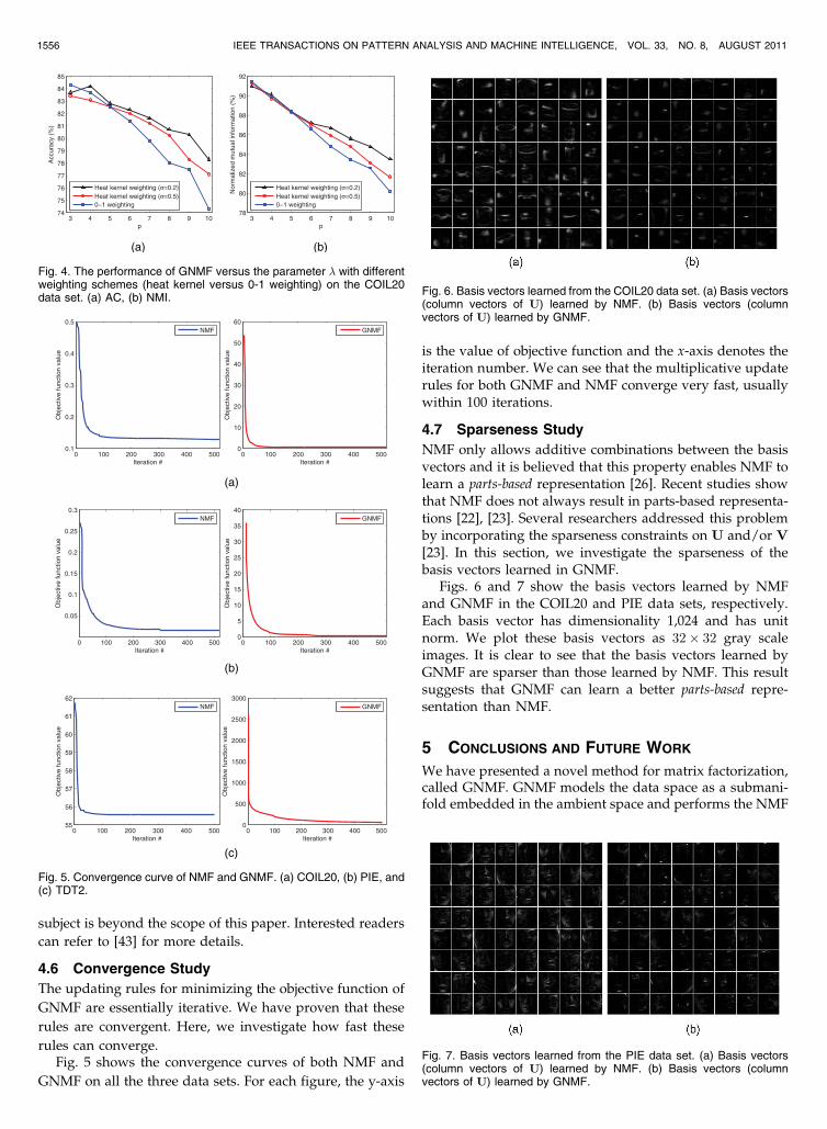
rules can converge.Fig. 5 shows the convergence curves of both NMF and
GNMF on all the three data sets. For each figure, the y-axis
is the value of objective function and the x-axis denotes theiteration number. We can see that the multiplicative updaterules for both GNMF and NMF converge very fast, usuallywithin 100 iterations.
4.7 Sparseness Study
NMF only allows additive combinations between the basisvectors and it is believed that this property enables NMF tolearn a parts-based representation [26]. Recent studies showthat NMF does not always result in parts-based representa-tions [22], [23]. Several researchers addressed this problemby incorporating the sparseness constraints on U and/or V
[23]. In this section, we investigate the sparseness of thebasis vectors learned in GNMF.
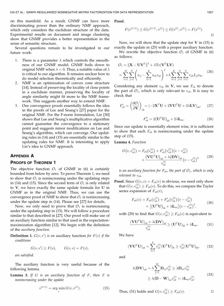
Figs. 6 and 7 show the basis vectors learned by NMFand GNMF in the COIL20 and PIE data sets, respectively.Each basis vector has dimensionality 1,024 and has unitnorm. We plot these basis vectors as 32� 32 gray scaleimages. It is clear to see that the basis vectors learned byGNMF are sparser than those learned by NMF. This resultsuggests that GNMF can learn a better parts-based repre-sentation than NMF.
5 CONCLUSIONS AND FUTURE WORK
We have presented a novel method for matrix factorization,called GNMF. GNMF models the data space as a submani-fold embedded in the ambient space and performs the NMF
1556 IEEE TRANSACTIONS ON PATTERN ANALYSIS AND MACHINE INTELLIGENCE, VOL. 33, NO. 8, AUGUST 2011
Fig. 5. Convergence curve of NMF and GNMF. (a) COIL20, (b) PIE, and(c) TDT2.
Fig. 6. Basis vectors learned from the COIL20 data set. (a) Basis vectors(column vectors of U) learned by NMF. (b) Basis vectors (columnvectors of U) learned by GNMF.
Fig. 7. Basis vectors learned from the PIE data set. (a) Basis vectors(column vectors of U) learned by NMF. (b) Basis vectors (columnvectors of U) learned by GNMF.
Fig. 4. The performance of GNMF versus the parameter � with differentweighting schemes (heat kernel versus 0-1 weighting) on the COIL20data set. (a) AC, (b) NMI.
on this manifold. As a result, GNMF can have morediscriminating power than the ordinary NMF approach,which only considers the euclidean structure of the data.Experimental results on document and image clusteringshow that GNMF provides a better representation in thesense of semantic structure.
Several questions remain to be investigated in ourfuture work:
1. There is a parameter � which controls the smooth-ness of our GNMF model. GNMF boils down tooriginal NMF when � ¼ 0. Thus, a suitable value of �is critical to our algorithm. It remains unclear how todo model selection theoretically and efficiently.
2. NMF is an optimization of convex cone structure[14]. Instead of preserving the locality of close pointsin a euclidean manner, preserving the locality ofangle similarity might fit more to the NMF frame-work. This suggests another way to extend NMF.
3. Our convergence proofs essentially follows the ideain the proofs of Lee and Seung’s [27] paper for theoriginal NMF. For the F-norm formulation, Lin [30]shows that Lee and Seung’s multiplicative algorithmcannot guarantee the convergence to a stationarypoint and suggests minor modifications on Lee andSeung’s algorithm, which can converge. Our updat-ing rules in (14) and (15) are essentially similar to theupdating rules for NMF. It is interesting to applyLin’s idea to GNMF approach.
APPENDIX A
PROOFS OF THEOREM 1
The objective function O1 of GNMF in (6) is certainlybounded from below by zero. To prove Theorem 1, we needto show that O1 is nonincreasing under the updating stepsin (14) and (15). Since the second term of O1 is only relatedto V, we have exactly the same update formula for U inGNMF as in the original NMF. Thus, we can use theconvergence proof of NMF to show that O1 is nonincreasingunder the update step in (14). Please see [27] for details.
Now, we only need to prove that O1 is nonincreasingunder the updating step in (15). We will follow a proceduresimilar to that described in [27]. Our proof will make use ofan auxiliary function similar to that used in the expectation-maximization algorithm [12]. We begin with the definitionof the auxiliary function.
Definition 1. Gðv; v0Þ is an auxiliary function for F ðvÞ if the
conditions
Gðv; v0Þ � F ðvÞ; Gðv; vÞ ¼ F ðvÞ;
are satisfied.
The auxiliary function is very useful because of thefollowing lemma.
Lemma 3. If G is an auxiliary function of F , then F isnonincreasing under the update
vðtþ1Þ ¼ arg minv
Gðv; vðtÞÞ: ð25Þ
Proof.
F ðvðtþ1ÞÞ Gðvðtþ1Þ; vðtÞÞ GðvðtÞ; vðtÞÞ ¼ F ðvðtÞÞ:ut
Now, we will show that the update step for V in (15) is
exactly the update in (25) with a proper auxiliary function.We rewrite the objective function O1 of GNMF in (6)
as follows:
O1 ¼ kX�UVTk2 þ �TrðVTLVÞ
¼XMi¼1
XNj¼1
xij �XKk¼1
uikvjk
!2
þ�XKk¼1
XNj¼1
XNl¼1
vjkLjlvlk:ð26Þ
Considering any element vab in V, we use Fab to denote
the part of O1, which is only relevant to vab. It is easy to
check that
F 0ab ¼@O1
@V
� �ab
¼ ð�2XTUþ 2VUTUþ 2�LVÞab; ð27Þ
F 00ab ¼ 2�UTU
�bbþ 2�Laa: ð28Þ
Since our update is essentially element wise, it is sufficient
to show that each Fab is nonincreasing under the update
step of (15).
Lemma 4. Function
G�v; vðtÞab
�¼ Fab
�vðtÞab
�þ F 0ab
�vðtÞab
��v� vðtÞab
�þ�VUTU
�abþ �
�DVÞab
vðtÞab
�v� vðtÞab
�2 ð29Þ
is an auxiliary function for Fab, the part of O1, which is only
relevant to vab.
Proof. Since Gðv; vÞ ¼ FabðvÞ is obvious, we need only show
that Gðv; vðtÞab Þ � FabðvÞ. To do this, we compare the Taylor
series expansion of FabðvÞ,
FabðvÞ ¼ Fab�vðtÞab
�þ F 0ab
�vðtÞab
��v� vðtÞab
�þ��
UTU�bbþ �Laa
��v� vðtÞab
�2;
ð30Þ
with (29) to find that Gðv; vðtÞab Þ � FabðvÞ is equivalent to
ðVUTUÞab þ �ðDVÞabvðtÞab
� ðUTUÞbb þ �Laa: ð31Þ
We have
ðVUTUÞab ¼Xkl¼1
vðtÞal ðUTUÞlb � v
ðtÞab ðUTUÞbb; ð32Þ
and
�ðDVÞab ¼ �XMj¼1
DajvðtÞjb � �Daav
ðtÞab
� �ðD�WÞaavðtÞab ¼ �Laav
ðtÞab :
ð33Þ
Thus, (31) holds and Gðv; vðtÞab Þ � FabðvÞ. tu
CAI ET AL.: GRAPH REGULARIZED NONNEGATIVE MATRIX FACTORIZATION FOR DATA REPRESENTATION 1557

We can now demonstrate the convergence of Theorem 1.
Proof of Theorem 1. Replacing Gðv; vðtÞab Þ in (25) by (29)
results in the update rule
vðtþ1Þab ¼ vðtÞab � v
ðtÞab
F 0ab�vðtÞab
�2ðVUTUÞab þ 2�ðDVÞab
¼ vðtÞabðXTUþ �WVÞabðVUTUþ �DVÞab
:
ð34Þ
Since (29) is an auxiliary function, Fab is nonincreasing
under this update rule. tu
APPENDIX B
PROOFS OF THEOREM 2
Similarly, the second term of O2 in (7) is only related to V;
we have exactly the same update formula for U in GNMF as
the original NMF. Thus, we can use the convergence proof
of NMF to show that O2 is nonincreasing under the update
step in (20). Please see [27] for details.Now, we will show that the update step for V in (21) is
exactly the update in (25) with a proper auxiliary function.
Lemma 5. Function
GðV;VðtÞÞ
¼Xi;j
xij logxij � xij þXKk¼1
uikvjk
!
�Xi;j;k
xij
uikvðtÞjkP
k uikvðtÞjk
�loguikvjk � log
uikvðtÞjkP
k uikvðtÞjk
�!
þ �2
Xj;l;k
vjk logvjkvlkþ vlk log
vlkvjk
� �Wjl;
is an auxiliary function for the objective function of GNMF in (7)
F ðVÞ ¼Xi;j
xij logxijPk uikvjk
� xij þXk
uikvjk
!
þ �2
Xj;l;k
vjk logvjkvlkþ vlk log
vlkvjk
� �Wjl:
Proof. It is straightforward to verify that GðV;VÞ ¼ F ðVÞ.To show that GðV;VðtÞÞ � F ðVÞ, we use convexity of the
log function to derive the inequality
� logXKk¼1
uikvjk
! �
XKk¼1
�k loguikvjk�k
� �;
which holds for all nonnegative �k that sum to unity.
Setting
�k ¼uikv
ðtÞjkPK
k¼1 uikvðtÞjk
;
we obtain
� logXk
uikvjk
!
�Xk
uikvðtÞjkP
k uikvðtÞjk
loguikvjk � loguikv
ðtÞjkP
k uikvðtÞjk
! !:
From this inequality, it follows that GðV;VðtÞÞ �F ðVÞ. tuTheorem 2, then follows from the application of Lemma 5:
Proof of Theorem 2. The minimum of GðV;VðtÞÞ with
respect to V is determined by setting the gradient to zero:
XMi¼1
uik �XMi¼1
xijuikv
ðtÞjkP
k uikvðtÞjk
1
vjk
þ �2
XNl¼1
logvjkvlkþ 1� vlk
vjk
� �Wjl ¼ 0
1 j N; 1 k K:
ð35Þ
Because of the log term, it is really hard to solve the
above system of equations. Let us recall the motivation of
the regularization term. We hope that if two data points
xj and xr are close (i.e., Wjr is big), zj will be close to zrand vjs=vrs will be approximately 1. Thus, we can use the
following approximation:
logðxÞ � 1� 1
x; x! 1:
The above approximation is based on the first order
expansion of Taylor series of the log function. With this
approximation, the equations in (35) can be written as
XMi¼1
uik�XMi¼1
xijuikv
ðtÞjkP
k uikvðtÞjk
1
vjk
þ �
vjk
XNl¼1
vjk � vlk� �
Wjl ¼ 0
1 j N; 1 k K:
ð36Þ
Let D denote a diagonal matrix whose entries are column
(or row, since W is symmetric) sums of W,
Djj ¼P
l Wjl. Define L ¼ D�W. Let vk denote the
kth column of V;vk ¼ ½v1k; . . . ; vNk�T . It is easy to verify
thatP
lðvjl � vlkÞWjl equals the jth element of vector Lvk.The system of equations in (36) can be rewritten as
Xi
uikIvk þ �Lvk ¼
vðtÞ1k
Pi xi1uik=
Pk uikv
ðtÞ1k
...
vðtÞNk
Pi xiNuik=
Pk uikv
ðtÞNk
266664
377775;
1 k K:
1558 IEEE TRANSACTIONS ON PATTERN ANALYSIS AND MACHINE INTELLIGENCE, VOL. 33, NO. 8, AUGUST 2011

Thus, the update rule of (25) takes the form
vðtþ1Þk ¼
Xi
uikIþ �L
!�1vðtÞ1k
Pi xi1uik=
Pk uikv
ðtÞ1k
...
vðtÞNk
Pi xiNuik=
Pk uikv
ðtÞNk
266664
377775;
1 k K:
Since G is an auxiliary function, F is nonincreasingunder this update. tu
APPENDIX C
WEIGHTED NMF AND GNMF
In this appendix, we provide a brief description of normal-ized cut weighted NMF, which was first introduced by Xuet al. [42]. Letting zTj be the jth row vector of V, the objectivefunction of NMF can be written as
O ¼XNj¼1
�xj �Uzj
�T �xj �Uzj
�;
which is the summation of the reconstruction errors over allof the data points, and each data point is equally weighted.If each data point has weight �j, the objective function ofweighted NMF can be written as
O0 ¼XNj¼1
�jðxj �UzjÞT ðxj �UzjÞ
¼ TrððX�UVT Þ�ðX�UVT ÞT Þ¼ TrððX�1=2 �UVT�1=2ÞðX�1=2 �UVT�1=2ÞT Þ¼ TrððX0 �UV0T ÞT ðX0 �UV0T ÞÞ;
where � is the diagonal matrix consists of �j, V0 ¼ �1=2V,and X0 ¼ X�1=2. Notice that the above equation has thesame form as (1) in Section 2 (the objective function ofNMF), so the same algorithm for NMF can be used to findthe solution of this weighted NMF problem. In [42], Xu et al.calculate D ¼ diagðXTXeÞ, where e is a vector of all ones.They use D�1 as the weight and named this approach asnormalized cut weighted NMF (NMF-NCW). The experi-mental results [42] have demonstrated the effectiveness ofthis weighted approach on document clustering.
Similarly, we can also introduce this weighting schemeinto our GNMF approach. The objective function ofweighted GNMF is
O0 ¼XNj¼1
�jðxj �UzjÞT ðxj �UzjÞ þ �TrðVTLVÞ
¼ TrððX�UVT Þ�ðX�UVT ÞT Þ þ �TrðVTLVÞ¼ TrððX�1=2 �UVT�1=2ÞðX�1=2 �UVT�1=2ÞT Þþ �TrðVTLVÞ¼ TrððX0 �UV0T ÞT ðX0 �UV0T ÞÞ þ �TrðV0TL0V0Þ;
where �;V0, and X0 are defined as before and L0 ¼��1=2L��1=2. Notice that the above equation has the same
form as (8) in Section 3.2, so the same algorithm for GNMF
can be used to find the solution of weighted GNMF problem.
ACKNOWLEDGMENTS
This work was supported in part by the National Natural
Science Foundation of China under Grants 60905001 and
90920303, the National Key Basic Research Foundation of
China under Grant 2009CB320801, US National Science
Foundation IIS-09-05215, and the US Army Research
Laboratory under Cooperative Agreement Number
W911NF-09-2-0053 (NS-CTA). Any opinions, findings, and
conclusions expressed here are those of the authors and do
not necessarily reflect the views of the funding agencies.
REFERENCES
[1] M. Belkin and P. Niyogi, “Laplacian Eigenmaps and SpectralTechniques for Embedding and Clustering,” Advances in NeuralInformation Processing Systems 14, pp. 585-591, MIT Press, 2001.
[2] M. Belkin, P. Niyogi, and V. Sindhwani, “Manifold Regulariza-tion: A Geometric Framework for Learning from Examples,”J. Machine Learning Research, vol. 7, pp. 2399-2434, 2006.
[3] J.-P. Brunet, P. Tamayo, T.R. Golub, and J.P. Mesirov, “Metagenesand Molecular Pattern Discovery Using Matrix Factorization,”Nat’l Academy of Sciences, vol. 101, no. 12, pp. 4164-4169, 2004.
[4] D. Cai, X. He, and J. Han, “Document Clustering Using LocalityPreserving Indexing,” IEEE Trans. Knowledge and Data Eng.,vol. 17, no. 12, pp. 1624-1637, Dec. 2005.
[5] D. Cai, X. He, X. Wang, H. Bao, and J. Han, “Locality PreservingNonnegative Matrix Factorization,” Proc. Int’l Joint Conf. ArtificialIntelligence, 2009.
[6] D. Cai, X. He, X. Wu, and J. Han, “Non-Negative MatrixFactorization on Manifold,” Proc. Int’l Conf. Data Mining, 2008.
[7] D. Cai, X. Wang, and X. He, “Probabilistic Dyadic Data Analysiswith Local and Global Consistency,” Proc. 26th Ann. Int’l Conf.Machine Learning, pp. 105-112, 2009.
[8] M. Catral, L. Han, M. Neumann, and R. Plemmons, “On ReducedRank Nonnegative Matrix Factorization for Symmetric Nonnega-tive Matrices,” Linear Algebra and Its Applications, vol. 393, pp. 107-126, 2004.
[9] F.R.K. Chung, Spectral Graph Theory. Am. Math. Soc., 1997.[10] T.H. Cormen, C.E. Leiserson, R.L. Rivest, and C. Stein, Introduction
to Algorithms, second ed. MIT Press and McGraw-Hill, 2001.[11] S.C. Deerwester, S.T. Dumais, T.K. Landauer, G.W. Furnas, and
R.A. harshman, “Indexing by Latent Semantic Analysis,” J. Am.Soc. of Information Science, vol. 41, no. 6, pp. 391-407, 1990.
[12] A.P. Dempster, N.M. Laird, and D.B. Rubin, “Maximum Like-lihood from Incomplete Data via the Em Algorithm,” J. RoyalStatistical Soc. Series B (Methodological), vol. 39, no. 1, pp. 1-38, 1977.
[13] C. Ding, T. Li, and W. Peng, “Nonnegative Matrix Factorizationand Probabilistic Latent Semantic Indexing: Equivalence, Chi-Square Statistic, and a Hybrid Method,” Proc. Nat’l Conf. AmericanAssociation for Artificial Intelligence, 2006.
[14] D. Donoho and V. Stodden, “When Does Non-Negative MatrixFactorization Give a Correct Decomposition into Parts?” Advancesin Neural Information Processing Systems 16, MIT Press, 2003.
[15] R.O. Duda, P.E. Hart, and D.G. Stork, Pattern Classification, seconded. Wiley-Interscience, 2000.
[16] L. Finesso and P. Spreij, “Nonnegative Matrix Factorization andI-Divergence Alternating Minimization,” Linear Algebra and ItsApplications, vol. 416, nos. 2/3, pp. 270-287, 2006.
[17] E. Gaussier and C. Goutte, “Relation between PLSA and NFM andImplications,” Proc. 28th Ann. Int’l ACM SIGIR Conf. Research andDevelopment in Information Retrieval, pp. 601-602, 2005.
[18] R. Hadsell, S. Chopra, and Y. LeCun, “Dimensionality Reductionby Learning an Invariant Mapping,” Proc. IEEE CS. Conf. ComputerVision and Pattern Recognition, pp. 1735-1742, 2006.
[19] X. He and P. Niyogi, “Locality Preserving Projections,” Advancesin Neural Information Processing Systems 16, MIT Press, 2003.
[20] M.R. Hestenes and E. Stiefel, “Methods of Conjugate Gradients forSolving Linear Systems,” J. Research of the Nat’l Bureau of Standards,vol. 49, no. 6, pp. 409-436, 1952.
CAI ET AL.: GRAPH REGULARIZED NONNEGATIVE MATRIX FACTORIZATION FOR DATA REPRESENTATION 1559

[21] T. Hofmann, “Unsupervised Learning by Probabilistic LatentSemantic Analysis,” Machine Learning, vol. 42, nos. 1/2, pp. 177-196, 2001.
[22] P.O. Hoyer, “Non-Negative Sparse Coding,” Proc. IEEE WorkshopNeural Networks for Signal Processing, pp. 557-565, 2002.
[23] P.O. Hoyer, “Non-Negative Matrix Factorization with SparsenessConstraints,” J. Machine Learning Research, vol. 5, pp. 1457-1469,2004.
[24] I.T. Jolliffe, Principal Component Analysis. Springer-Verlag, 1989.[25] J. Kivinen and M.K. Warmuth, “Additive versus Exponentiated
Gradient Updates for Linear Prediction,” Proc. Ann. ACM Symp.Theory of Computing, pp. 209-218, 1995.
[26] D.D. Lee and H.S. Seung, “Learning the Parts of Objects by Non-Negative Matrix Factorization,” Nature, vol. 401, pp. 788-791, 1999.
[27] D.D. Lee and H.S. Seung, “Algorithms for Non-Negative MatrixFactorization,” Advances in Neural Information Processing Systems13, MIT Press, 2001.
[28] J.M. Lee, Introduction to Smooth Manifolds. Springer-Verlag, 2002.[29] S.Z. Li, X. Hou, H. Zhang, and Q. Cheng, “Learning Spatially
Localized, Parts-Based Representation,” Proc. IEEE CS Conf.Computer Vision and Pattern Recognition, pp. 207-212, 2001.
[30] C.-J. Lin, “On the Convergence of Multiplicative Update Algo-rithms for Non-Negative Matrix Factorization,” IEEE Trans. NeuralNetworks, vol. 18, no. 6, pp. 1589-1596, Nov. 2007.
[31] N.K. Logothetis and D.L. Sheinberg, “Visual Object Recognition,”Ann. Rev. of Neuroscience, vol. 19, pp. 577-621, 1996.
[32] A.Y. Ng, M. Jordan, and Y. Weiss, “On Spectral Clustering:Analysis and an Algorithm,” Advances in Neural InformationProcessing Systems 14, pp. 849-856, MIT Press, 2001.
[33] P. Paatero and U. Tapper, “Positive Matrix Factorization: A Non-Negative Factor Model with Optimal Utilization of ErrorEstimates of Data Values,” Environmetrics, vol. 5, no. 2, pp. 111-126, 1994.
[34] S.E. Palmer, “Hierarchical Structure in Perceptual Representa-tion,” Cognitive Psychology, vol. 9, pp. 441-474, 1977.
[35] S. Roweis and L. Saul, “Nonlinear Dimensionality Reduction byLocally Linear Embedding,” Science, vol. 290, no. 5500, pp. 2323-2326, 2000.
[36] H.S. Seung and D.D. Lee, “The Manifold Ways of Perception,”Science, vol. 290, no. 12, pp. 2268/2269, 2000.
[37] F. Shahnaza, M.W. Berrya, V. Paucab, and R.J. Plemmonsb,“Document Clustering Using Nonnegative Matrix Factorization,”Information Processing and Management, vol. 42, no. 2, pp. 373-386,2006.
[38] J. Shi and J. Malik, “Normalized Cuts and Image Segmentation,”IEEE Trans. Pattern Analysis and Machine Intelligence, vol. 22, no. 8,pp. 888-905, Aug. 2000.
[39] J. Tenenbaum, V. de Silva, and J. Langford, “A Global GeometricFramework for Nonlinear Dimensionality Reduction,” Science,vol. 290, no. 5500, pp. 2319-2323, 2000.
[40] M. Turk and A. Pentland, “Eigenfaces for Recognition,”J. Cognitive Neuroscience, vol. 3, no. 1, pp. 71-86, 1991.
[41] E. Wachsmuth, M.W. Oram, and D.I. Perrett, “Recognition ofObjects and Their Component Parts: Responses of Single Units inthe Temporal Cortex of the Macaque,” Cerebral Cortex, vol. 4,pp. 509-522, 1994.
[42] W. Xu, X. Liu, and Y. Gong, “Document Clustering Based on Non-Negative Matrix Factorization,” Proc. Ann. Int’l ACM SIGIR Conf.Research and Development in Information Retrieval, pp. 267-273, Aug.2003.
[43] L. Zelnik-Manor and P. Perona, “Self-Tuning Spectral Clustering,”Advances in Neural Information Processing Systems 17, pp. 1601-1608,MIT Press, 2004.
[44] H. Zha, C. Ding, M. Gu, X. He, and H. Simon, “Spectral Relaxationfor k-Means Clustering,” Advances in Neural Information ProcessingSystems 14, pp. 1057-1064, MIT Press, 2001.
[45] D. Zhou, O. Bousquet, T. Lal, J. Weston, and B. Scholkopf,“Learning with Local and Global Consistency,” Advances in NeuralInformation Processing Systems 16, MIT Press, 2003.
[46] X. Zhu and J. Lafferty, “Harmonic Mixtures: Combining MixtureModels and Graph-Based Methods for Inductive and ScalableSemi-Supervised Learning,” Proc. 22nd Int’l Conf. Machine Learn-ing, pp. 1052-1059, 2005.
Deng Cai received the bachelor’s and master’sdegrees from Tsinghua University in 2000 and2003, respectively, both in automation. Hereceived the PhD degree in computer sciencefrom the University of Illinois at UrbanaChampaign in 2009. He is an associateprofessor in the State Key Lab of CAD&CG,College of Computer Science at ZhejiangUniversity, China. His research interests in-clude machine learning, data mining, and
information retrieval. He is a member of the IEEE.
Xiaofei He received the BS degree in computerscience from Zhejiang University, China, in2000, and the PhD degree in computer sciencefrom the University of Chicago in 2005. He is aprofessor in the State Key Lab of CAD&CG atZhejiang University, China. Prior to joiningZhejiang University, he was a research scientistat Yahoo! Research Labs, Burbank, California.His research interests include machine learning,information retrieval, and computer vision. He is
a senior member of the IEEE.
Jiawei Han is a professor of computer scienceat the University of Illinois. He has chaired orserved on more than 100 program committees ofthe major international conferences in the fieldsof data mining and database systems, and alsoserved or is serving on the editorial boards forData Mining and Knowledge Discovery, theIEEE Transactions on Knowledge and DataEngineering, the Journal of Computer Scienceand Technology, and the Journal of Intelligent
Information Systems. He is the founding editor-in-chief of the ACMTransactions on Knowledge Discovery from Data (TKDD). He hasreceived IBM Faculty Awards, HP Innovation Awards, the ACM SIGKDDInnovation Award (2004), the IEEE Computer Society TechnicalAchievement Award (2005), and the IEEE W. Wallace McDowell Award(2009). He is currently the director of the Information Network AcademicResearch Center (INARC) supported by the Network Science-Colla-borative Technology Alliance (NS-CTA) program of US Army ResearchLab. His book Data Mining: Concepts and Techniques (MorganKaufmann) has been used worldwide as a textbook. He is a fellow ofthe ACM and IEEE.
Thomas S. Huang received the ScD degreefrom the Massachusetts Institute of Technologyin electrical engineering, and was on the facultyof MIT and Purdue University. He joined theUniversity of Illinois at Urbana Champaign in1980 and is currently the William L. EverittDistinguished Professor of Electrical and Com-puter Engineering, a research professor in theCoordinated Science Laboratory, a professor inthe Center for Advanced Study, and cochair of
the Human Computer Intelligent Interaction major research theme of theBeckman Institute for Advanced Science and Technology. He is amember of the National Academy of Engineering and has receivednumerous honors and awards, including the IEEE Jack S. Kilby SignalProcessing Medal (with Ar. Netravali) and the King-Sun Fu Prize of theInternational Association of Pattern Recognition. He has published21 books and more than 600 technical papers in network theory, digitalholography, image and video compression, multimodal human computerinterfaces, and multimedia databases. He is a fellow of the IEEE.
. For more information on this or any other computing topic,please visit our Digital Library at www.computer.org/publications/dlib.
1560 IEEE TRANSACTIONS ON PATTERN ANALYSIS AND MACHINE INTELLIGENCE, VOL. 33, NO. 8, AUGUST 2011


![Some Recent Advances in Nonnegative Matrix Factorization and … · 2013. 11. 21. · [GG10] G., Glineur, Using Underapproximations for Sparse Nonnegative Matrix Factorization, Pattern](https://img.pdfslide.us/doc/110x75/5fe39a16fd4e890a280aa921/some-recent-advances-in-nonnegative-matrix-factorization-and-2013-11-21-gg10.jpg)

![Nonnegative Tensor Factorization for Source Separation of ... · [Rafii, Liutkus, & Pardo 2014] NMF can handle many types of repetition: Method. Nonnegative tensor factorization](https://img.pdfslide.us/doc/110x75/5f73cd6a4279576c155c076c/nonnegative-tensor-factorization-for-source-separation-of-raii-liutkus.jpg)