Embed Size (px)
Citation preview
Graph-based Semi-supervised Learning
Zoubin Ghahramani
Department of EngineeringUniversity of Cambridge, UK
[email protected]://learning.eng.cam.ac.uk/zoubin/
MLSS 2012La Palma
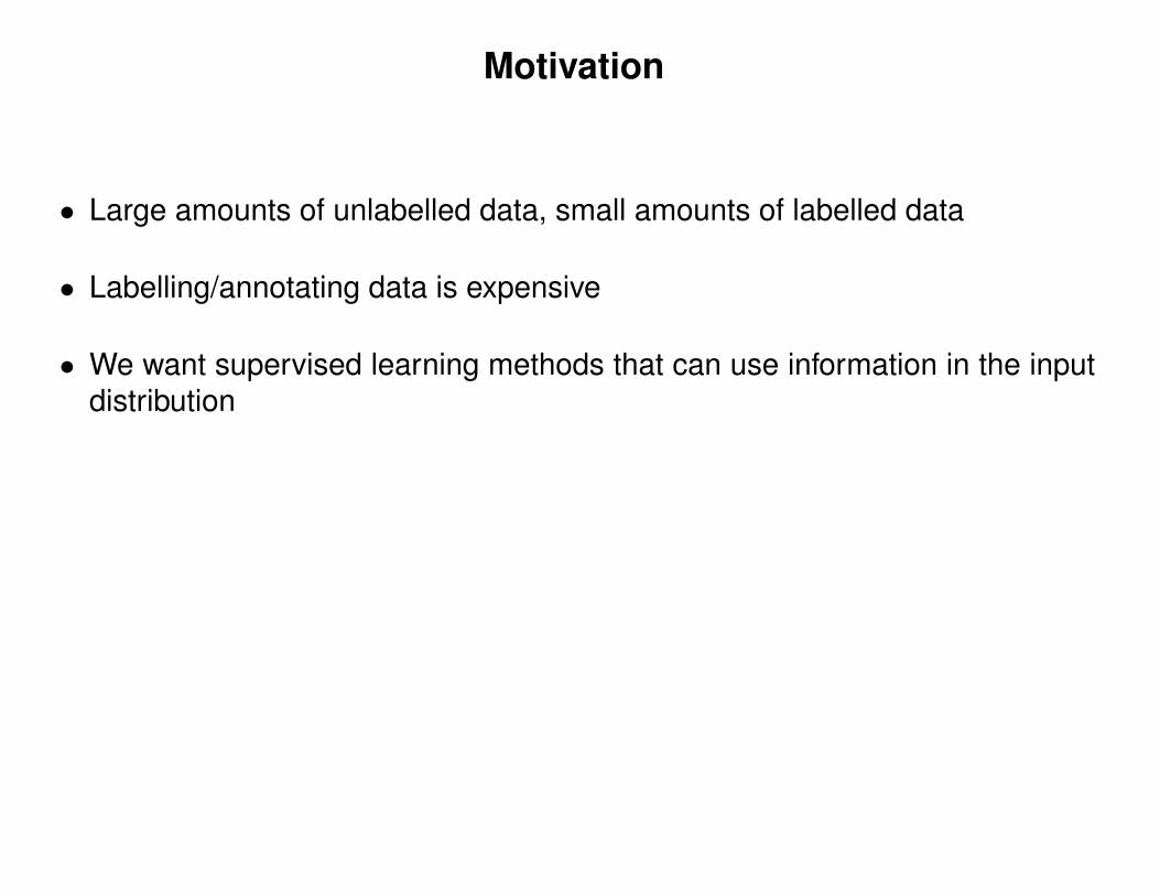
Motivation
• Large amounts of unlabelled data, small amounts of labelled data
• Labelling/annotating data is expensive
• We want supervised learning methods that can use information in the inputdistribution
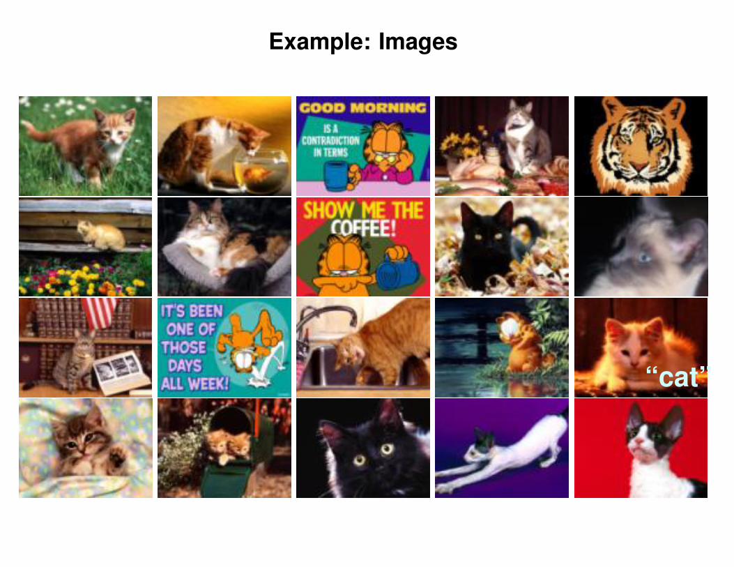
Example: Images
“cat”
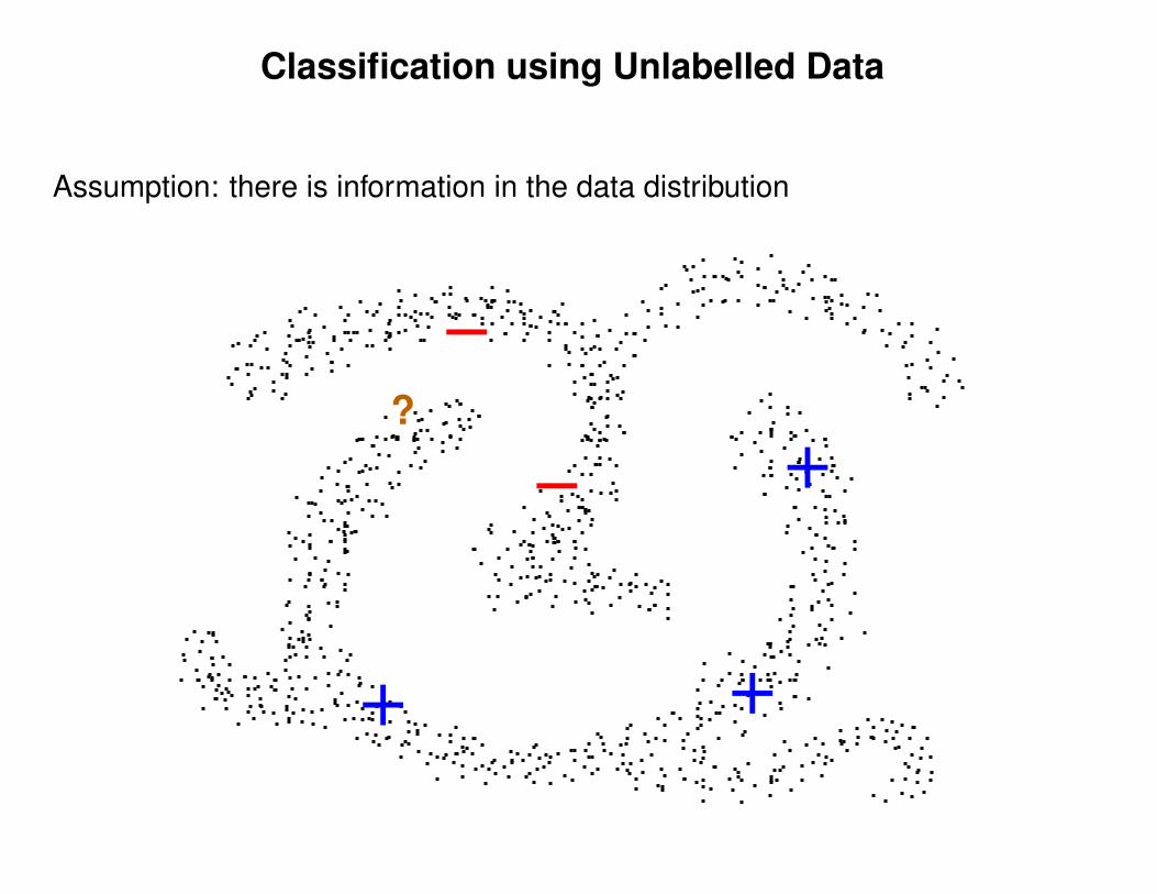
Classification using Unlabelled Data
Assumption: there is information in the data distribution
+ +
+
−
−
?
Outline
• Graph-based semi-supervised learning
• Active graph-based semi-supervised learning
• Some thoughts on Bayesian semi-supervised learning
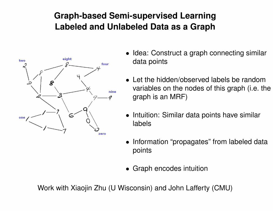
Graph-based Semi-supervised LearningLabeled and Unlabeled Data as a Graph
• Idea: Construct a graph connecting similardata points
• Let the hidden/observed labels be randomvariables on the nodes of this graph (i.e. thegraph is an MRF)
• Intuition: Similar data points have similarlabels
• Information “propagates” from labeled datapoints
• Graph encodes intuition
Work with Xiaojin Zhu (U Wisconsin) and John Lafferty (CMU)
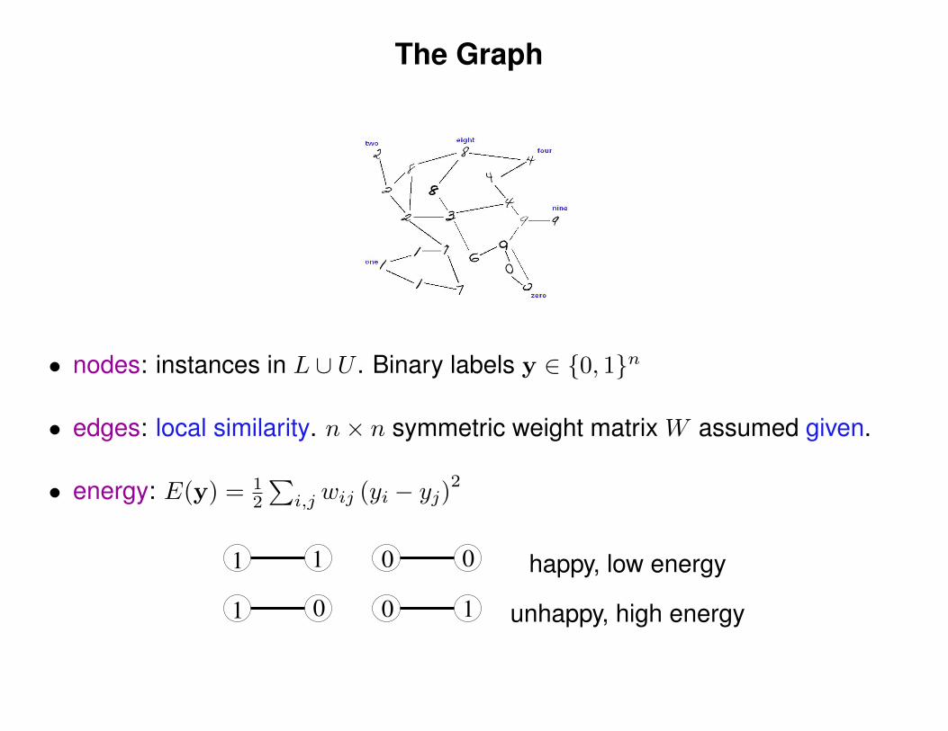
The Graph
• nodes: instances in L ∪ U . Binary labels y ∈ {0, 1}n
• edges: local similarity. n× n symmetric weight matrix W assumed given.
• energy: E(y) = 12
∑i,j wij (yi − yj)2
1 1 0 0 happy, low energy
1 00 1 unhappy, high energy
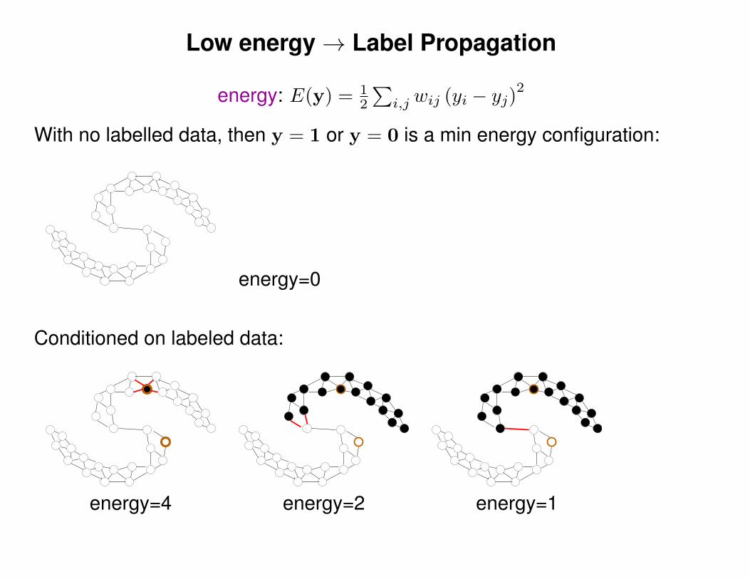
Low energy→ Label Propagation
energy: E(y) = 12
∑i,j wij (yi − yj)2
With no labelled data, then y = 1 or y = 0 is a min energy configuration:
energy=0
Conditioned on labeled data:
energy=4 energy=2 energy=1
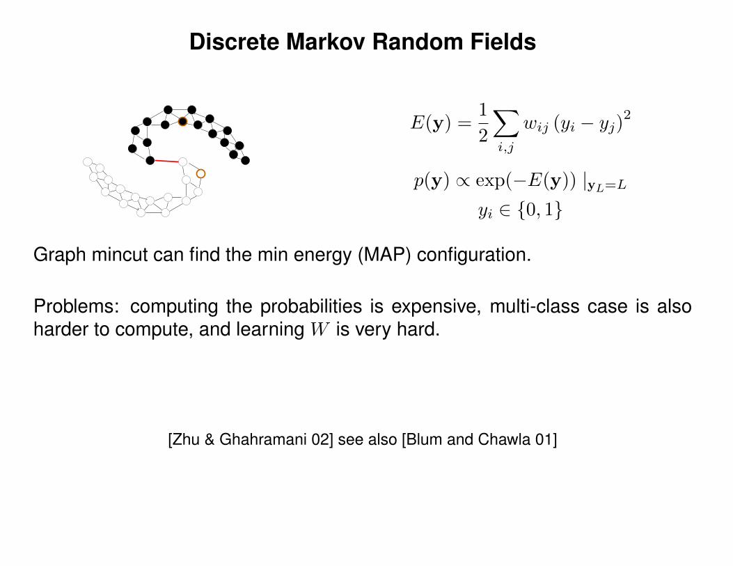
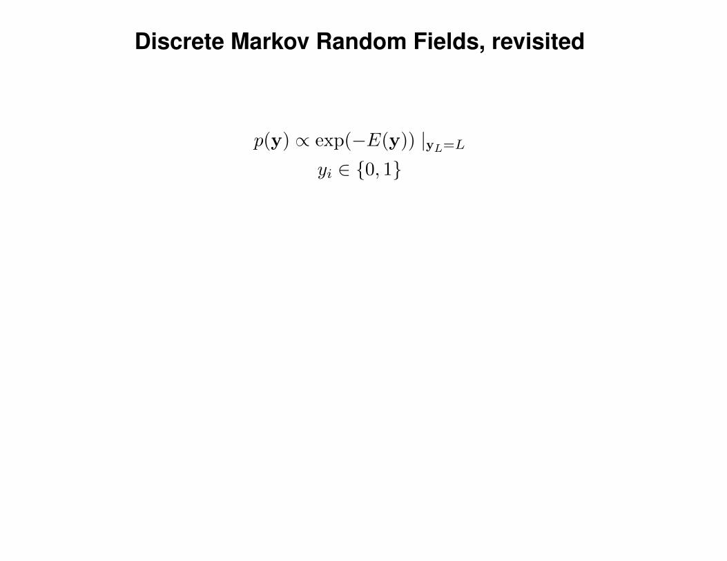
Discrete Markov Random Fields
E(y) =1
2
∑
i,j
wij (yi − yj)2
p(y) ∝ exp(−E(y)) |yL=Lyi ∈ {0, 1}
Graph mincut can find the min energy (MAP) configuration.
Problems: computing the probabilities is expensive, multi-class case is alsoharder to compute, and learning W is very hard.
[Zhu & Ghahramani 02] see also [Blum and Chawla 01]
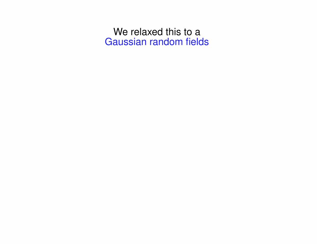
We relaxed this to aGaussian random fields
Discrete Markov Random Fields, revisited
p(y) ∝ exp(−E(y)) |yL=Lyi ∈ {0, 1}
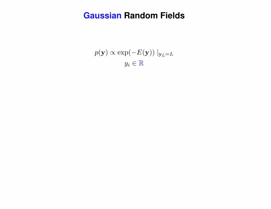
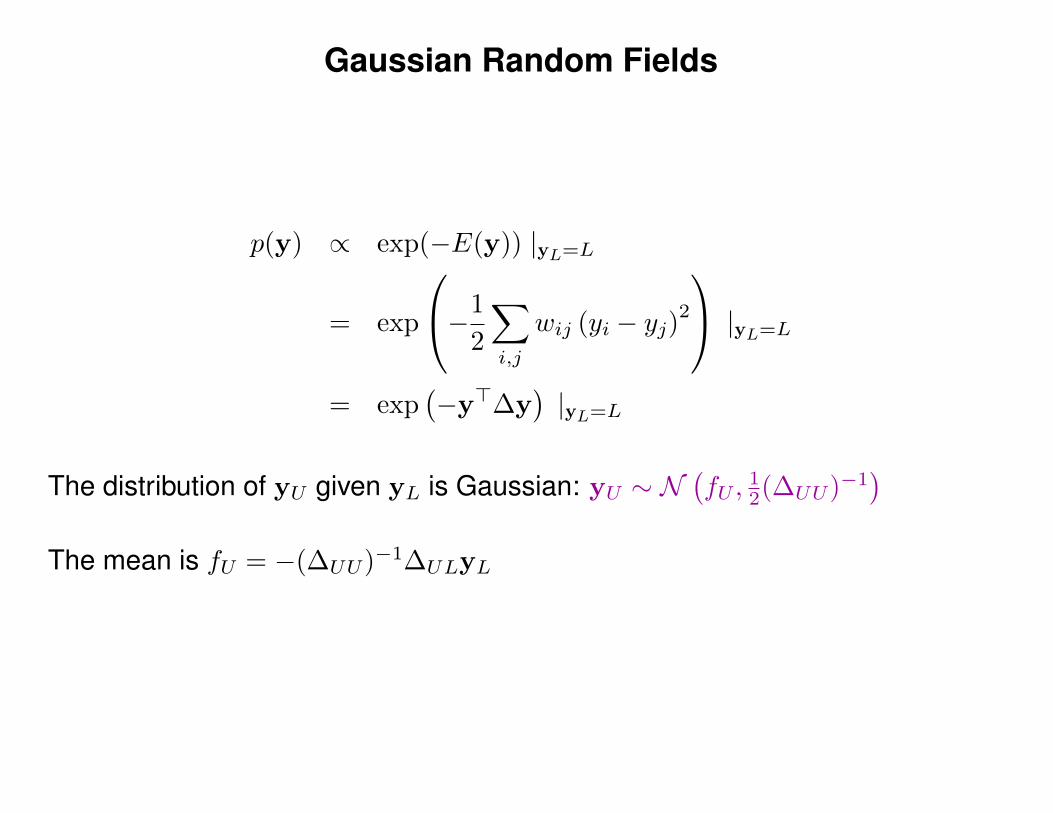
Gaussian Random Fields
p(y) ∝ exp(−E(y)) |yL=Lyi ∈ R
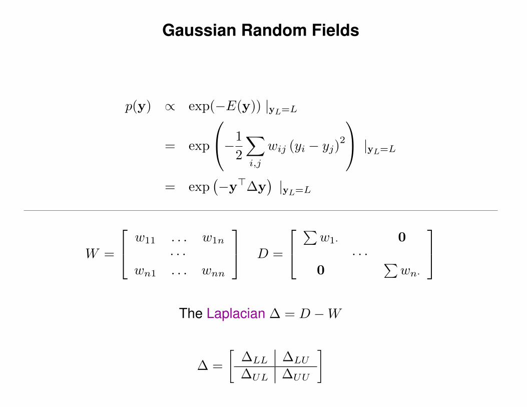
Gaussian Random Fields
p(y) ∝ exp(−E(y)) |yL=L
= exp
−1
2
∑
i,j
wij (yi − yj)2 |yL=L
= exp(−y>∆y
)|yL=L
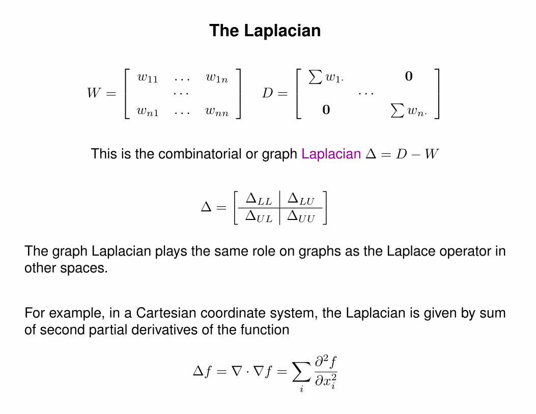
W =
w11 . . . w1n
· · ·wn1 . . . wnn
D =
∑w1· 0
· · ·0
∑wn·
The Laplacian ∆ = D −W
∆ =
[∆LL ∆LU
∆UL ∆UU
]
The Laplacian
W =
w11 . . . w1n
· · ·wn1 . . . wnn
D =
∑w1· 0
· · ·0
∑wn·
This is the combinatorial or graph Laplacian ∆ = D −W
∆ =
[∆LL ∆LU
∆UL ∆UU
]
The graph Laplacian plays the same role on graphs as the Laplace operator inother spaces.
For example, in a Cartesian coordinate system, the Laplacian is given by sumof second partial derivatives of the function
∆f = ∇ · ∇f =∑
i
∂2f
∂x2i
Gaussian Random Fields
p(y) ∝ exp(−E(y)) |yL=L
= exp
−1
2
∑
i,j
wij (yi − yj)2 |yL=L
= exp(−y>∆y
)|yL=L
The distribution of yU given yL is Gaussian: yU ∼ N(fU ,
12(∆UU)−1
)
The mean is fU = −(∆UU)−1∆ULyL
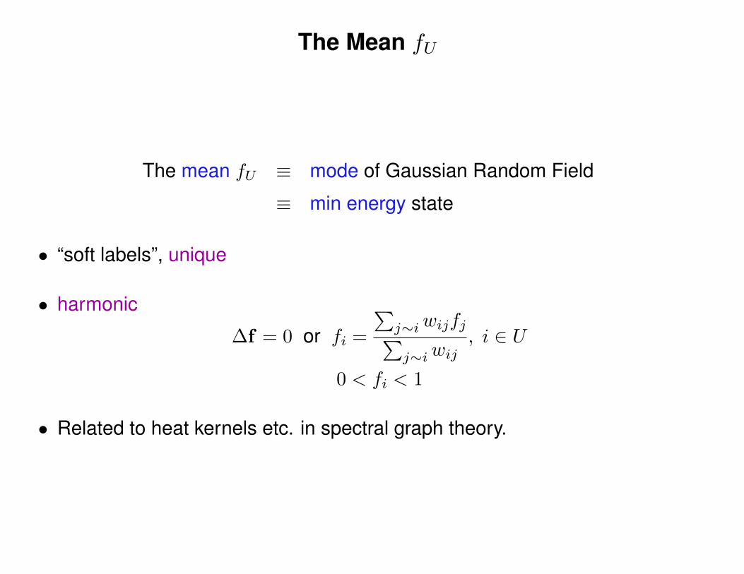
The Mean fU
The mean fU ≡ mode of Gaussian Random Field
≡ min energy state
• “soft labels”, unique
• harmonic
∆f = 0 or fi =
∑j∼iwijfj∑j∼iwij
, i ∈ U
0 < fi < 1
• Related to heat kernels etc. in spectral graph theory.
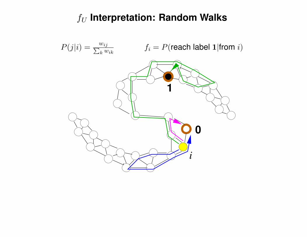
fU Interpretation: Random Walks
P (j|i) =wij∑k wik
fi = P (reach label 1|from i)
1
0
i
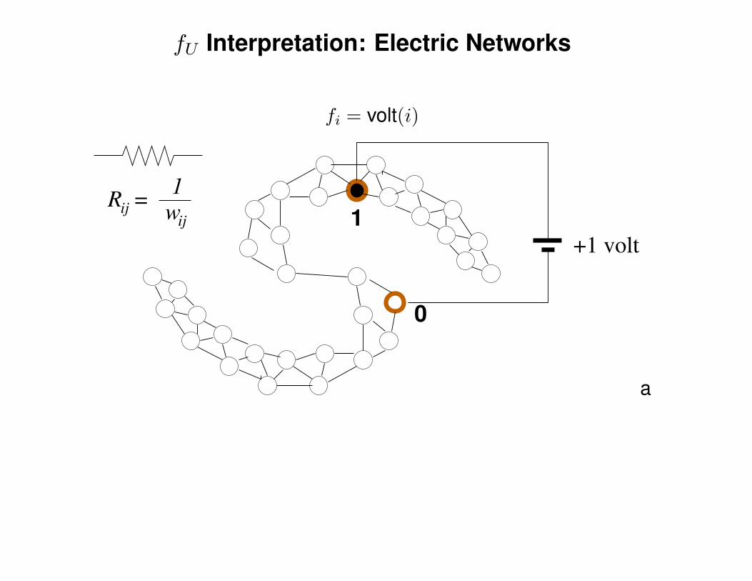
fU Interpretation: Electric Networks
fi = volt(i)
+1 volt
wij
R =ij
1
1
0
a
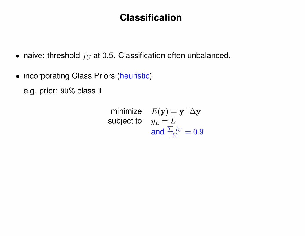
Classification
• naive: threshold fU at 0.5. Classification often unbalanced.
• incorporating Class Priors (heuristic)
e.g. prior: 90% class 1
minimize E(y) = y>∆ysubject to yL = L
and∑fU|U | = 0.9
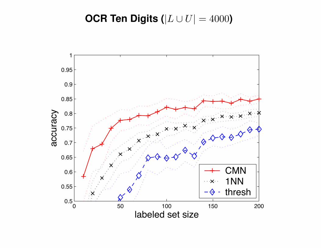
OCR Ten Digits (|L ∪ U | = 4000)
0 50 100 150 2000.5
0.55
0.6
0.65
0.7
0.75
0.8
0.85
0.9
0.95
1
labeled set size
accu
racy
CMN1NNthresh
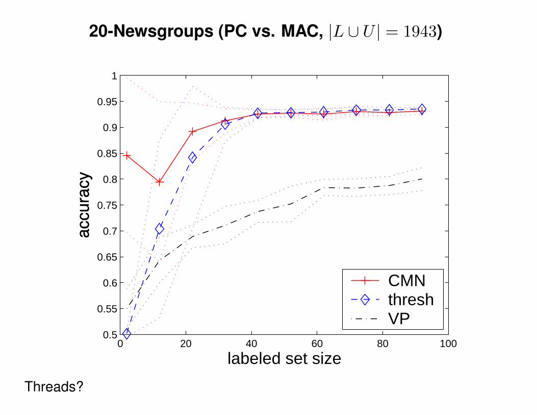
20-Newsgroups (PC vs. MAC, |L ∪ U | = 1943)
0 20 40 60 80 1000.5
0.55
0.6
0.65
0.7
0.75
0.8
0.85
0.9
0.95
1
labeled set size
accu
racy
CMNthreshVP
Threads?
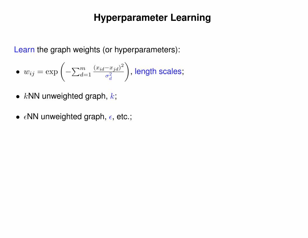
Hyperparameter Learning
Learn the graph weights (or hyperparameters):
• wij = exp
(−∑m
d=1
(xid−xjd)2σ2d
), length scales;
• kNN unweighted graph, k;
• εNN unweighted graph, ε, etc.;
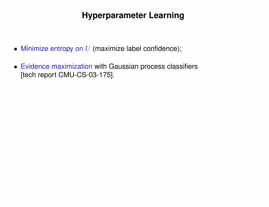
Hyperparameter Learning
• Minimize entropy on U (maximize label confidence);
• Evidence maximization with Gaussian process classifiers[tech report CMU-CS-03-175].
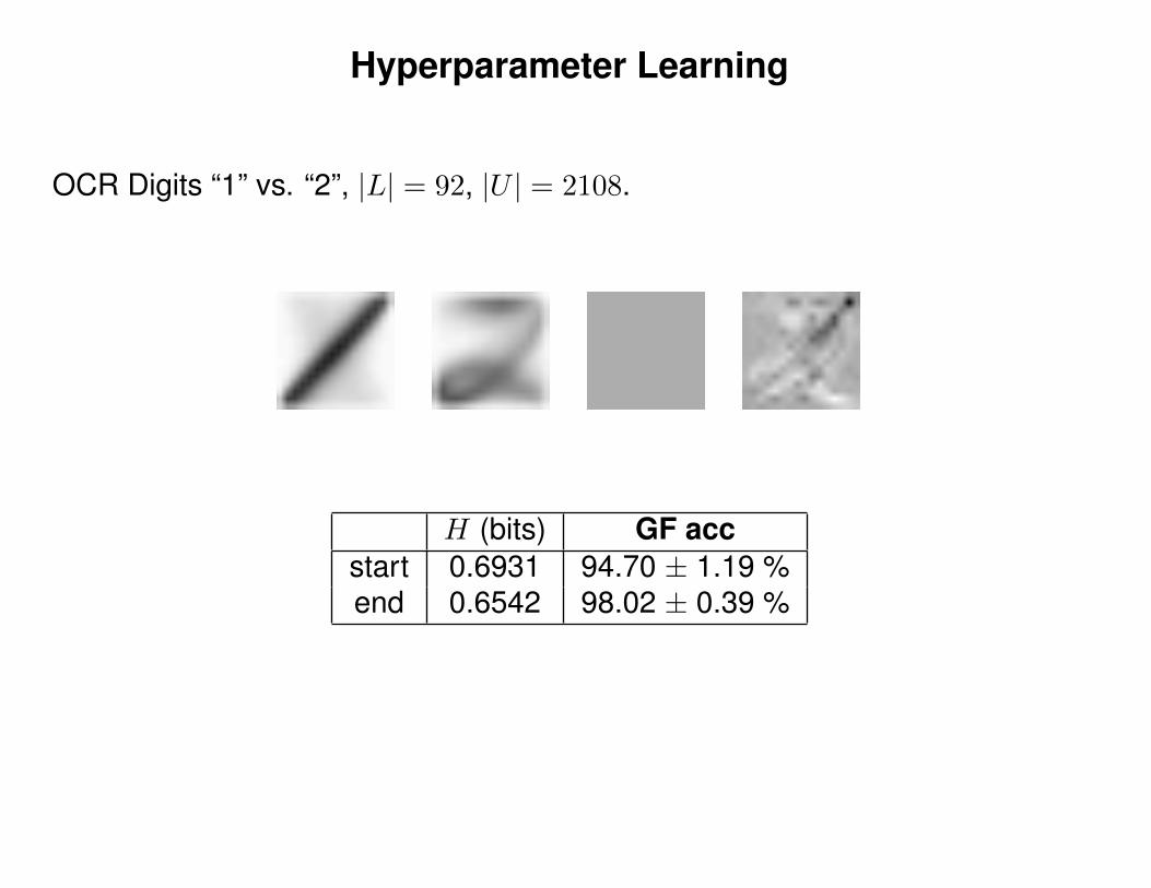
Hyperparameter Learning
OCR Digits “1” vs. “2”, |L| = 92, |U | = 2108.
H (bits) GF accstart 0.6931 94.70 ± 1.19 %end 0.6542 98.02 ± 0.39 %
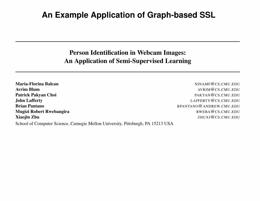
An Example Application of Graph-based SSL
Person Identification in Webcam Images:An Application of Semi-Supervised Learning
Maria-Florina Balcan [email protected] Blum [email protected] Pakyan Choi [email protected] Lafferty [email protected] Pantano [email protected] Robert Rwebangira [email protected] Zhu [email protected] of Computer Science, Carnegie Mellon University, Pittsburgh, PA 15213 USA
AbstractAn application of semi-supervised learning ismade to the problem of person identification inlow quality webcam images. Using a set of im-ages of ten people collected over a period of fourmonths, the person identification task is posedas a graph-based semi-supervised learning prob-lem, where only a few training images are la-beled. The importance of domain knowledgein graph construction is discussed, and experi-ments are presented that clearly show the advan-tage of semi-supervised learning over standardsupervised learning. The data used in the studyis available to the research community to encour-age further investigation of this problem.
1. IntroductionThe School of Computer Science at Carnegie Mellon Uni-versity has a public lounge, where leftover pizza and otherfood items from various meetings converge, to the delightof students, staff, and faculty. To help monitor the pres-ence of food in the lounge, a webcam, sometimes called theFreeFoodCam1, is mounted in a coke machine and trainedupon the table where food is placed. After being spottedon the webcam, the arrival of (almost) fresh free food isheralded with instant messages sent throughout the School.
The FreeFoodCam offers interesting opportunities for re-1http://www.cs.cmu.edu/˜coke, Carnegie Mellon
University internal
Appearing in Proc. of the 22 st ICML Workshop on Learning withPartially Classified Training Data, Bonn, Germany, 2005. Copy-right 2005 by the author(s)/owner(s).
search in semi-supervised machine learning. This paperpresents an investigation of the problem of person identi-fication in this low quality video data, using webcam im-ages of ten people that were collected over a period of sev-eral months. The results highlight the importance of do-main knowledge in semi-supervised learning, and clearlydemonstrate the advantages of using both labeled and unla-beled data over standard supervised learning.
In recent years, there has been a substantial amount of workexploring how best to incorporate unlabeled data into su-pervised learning (Zhu, 2005). Several semi-supervisedlearning approaches have been proposed for practical ap-plications in different areas, such as information retrieval,text classification (Nigam et al., 1998), and bioinformat-ics (Weston et al., 2004; Shin et al., 2004). In the contextof computer vision, several interesting results have beenobtained for object detection. Levin et al. (2003) intro-duced a technique based on co-training (Blum & Mitchell,1998) for fitting visual detectors in a way that requires onlya small quantity of labeled data, using unlabeled data toimprove performance over time. Rosenberg et al. (2005)present a semi-supervised approach to training object de-tection systems based on self-training, and perform exten-sive experiments with a state-of-the-art detector (Schnei-derman & Kanade, 2002; Schneiderman, 2004a; Schnei-derman, 2004b) demonstrating that a model trained in thismanner can achieve results comparable to a model trainedin the traditional manner using a much larger set of fullylabeled data.
In this work, we describe a new application of semi-supervised learning to the problem of person identificationin webcam images, where the video stream has a low framerate, and the images are of low quality. Significantly, manyof the images may have no face, as the person could be fac-ing away from the camera. We discuss the creation of the
The FreeFoodCam
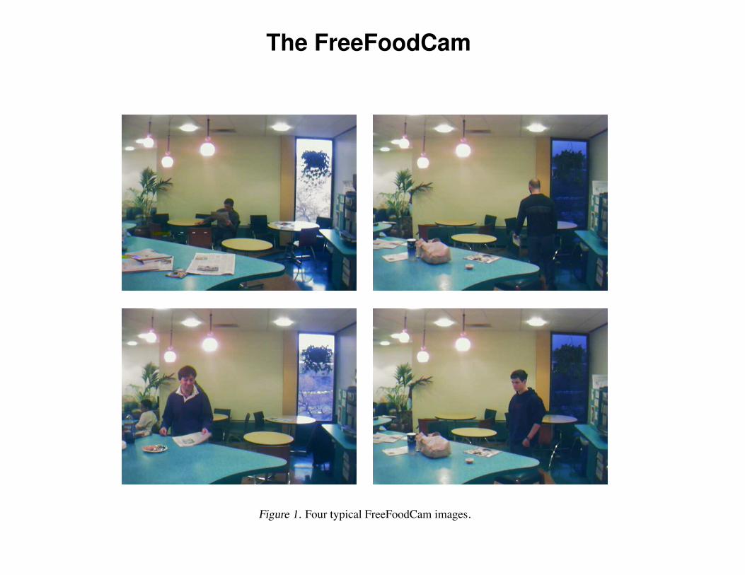
Figure 1. Four typical FreeFoodCam images.
dataset, and the formulation of the semi-supervised learn-ing problem. The task of face recognition, of course, hasan extensive literature; see (Zhao et al., 2003) for a sur-vey. However, to the best of our knowledge, person identi-fication in video data has not been previously attacked us-ing semi-supervised learning methods. Relatively primitiveimage processing techniques are used in our work; we notethat more sophisticated computer vision techniques can beeasily incorporated into the framework, and should onlyimprove the performance. But the spirit of our contributionis to argue that semi-supervised learning methods may beattractive as a complementary tool to advanced image pro-cessing. The data we have developed and that forms thebasis for the experiments reported here will be made avail-able to the research community.2
2. The FreeFoodCam DatasetThe dataset consists of 5254 images with one and only oneperson in it. Figure 1 shows four typical images from thedata. The task is not trivial:
• The images of each person were captured on multi-ple days during a four month period. People changed
2Instructions for obtaining the dataset can be found at http://www.cs.cmu.edu/˜zhuxj/freefoodcam.
clothes, hair styles, and one person even grew a beard.We simulate a video surveillance scenario where im-ages for a group of people are manually labeled in afew beginning frames, and the people must be recog-nized on later days. Therefore we choose labeled datawithin the first day of a person’s appearance, and teston the remaining images of the day and all other days.This is much more difficult than testing only on thesame day, or allowing labeled data to come from alldays.
• The FreeFoodCam is a low quality webcam. Eachframe has 640 ! 480 resolution so faces of far awaypeople are small. The frame rate is a little over 0.5frames per second, and lighting in the lounge is com-plex and changing.
• A person could turn their face away from the camera,and roughly one third of the images contain no face atall.
Since only a few images are labeled, and all of the test im-ages are available, the task is a natural candidate for theapplication of semi-supervised learning techniques.
Background Extraction
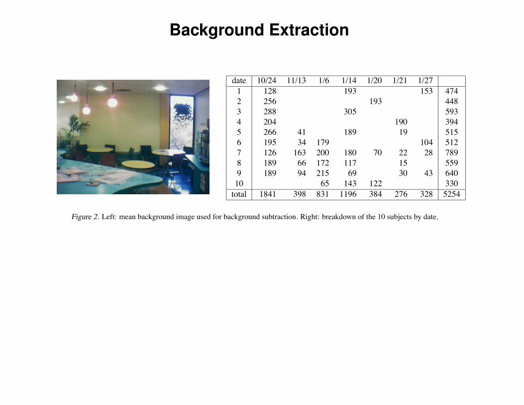
date 10/24 11/13 1/6 1/14 1/20 1/21 1/271 128 193 153 4742 256 193 4483 288 305 5934 204 190 3945 266 41 189 19 5156 195 34 179 104 5127 126 163 200 180 70 22 28 7898 189 66 172 117 15 5599 189 94 215 69 30 43 64010 65 143 122 330total 1841 398 831 1196 384 276 328 5254
Figure 2. Left: mean background image used for background subtraction. Right: breakdown of the 10 subjects by date.
2.1. Data Collection
We asked ten volunteers to appear in seven FreeFoodCamtakes over four months. Not all participants could show upfor every take. The FreeFoodCam is located in the Com-puter Science lounge, but we received a live camera feedin our office, and took images from the camera whenever anew frame was available.
In each take, the participants took turns entering the scene,walking around, and “acting naturally,” for example byreading the newspaper or chatting with off-camera col-leagues, for five to ten minutes per take. As a result, wecollected images where the individuals have varying posesand are at a range of distances from the camera. We dis-carded all frames that were corrupted by electronic noise inthe coke machine, or that contained more than one personin the scene. This latter constraint imposed was to makethe task simple to specify as a first step; there is no reasonthat the methods we present below could not be extendedto work with scenes containing multiple people.
2.2. Foreground Color Extraction
To accurately capture the color information of an individualin the image, based primarily on their clothing, we had toseparate him or her from the background. As computervision is not the focus of the work, we used only primitiveimage processing methods.
A simple background subtraction algorithm was used tofind the foreground. We computed the per-pixel meansand variances of red, green and blue channels from 294background images. Figure 2 shows the mean background.Using the means and variances of the background, we ob-tained the foreground area in each image by thresholding.Pixels deviating more than three standard derivations fromthe mean were treated as foreground.
To improve the quality of the foreground color histogram,
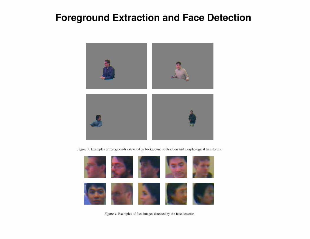
we processed the foreground area using morphologicaltransforms (Jain, 1989). Further processing was requiredbecause the foreground derived from background subtrac-tion often captured only part of the body and containedbackground areas. We first removed small islands in theforeground by applying the open operation with a 7 pixel-wide square. We then connected vertically-separated pixelblocks (such as head and lower torso) using the close opera-tion with a 60-pixel-by-10-pixel rectangular block. Finally,we made sure the foreground contains the entire person byenlarging the foreground to include neighboring pixels byfurther closing the foreground with a disk of 20 pixels inradius. And because there is only one person in each im-age, we discarded all but the largest contiguous block ofpixels in the processed foreground. Figure 3 shows someprocessed foreground images.
After this processing the foreground area is representedby a 100-dimensional vector, which consists of a 50-binhue histogram, a 30-bin saturation histogram, and a 20-binbrightness histogram.
2.3. Face Image Extraction
The face of the person is stored as a small image, whichis derived from the outputs of a face detector (Schneider-man 2004a; 2004b) . Note that this is not a face recognizer(a face recognizer was not used for this task). It simply de-tects the presence of frontal or profile faces, and outputs theestimated center and radius of the detected face. We took asquare area around the center as the face image. If no facewas detected, the face image is empty. Figure 4 shows afew face images as determined by the face detector.
2.4. Summary of the Dataset
In summary, the dataset is comprised of 5254 images forten individuals, collected during seven takes over fourmonths. There is a slight imbalance in the class distribu-
Foreground Extraction and Face Detection
Figure 3. Examples of foregrounds extracted by background subtraction and morphological transforms.
Figure 4. Examples of face images detected by the face detector.
tion, and only a subset of individuals are present in eachday (refer to Table 2 for the breakdown). Overall 34% ofthe images (1808 out of 5254) do not contain a face.
Each image in the dataset is represented by three features:
Time: The date and time the image was taken.
Color histogram of processed foreground: A 100 di-mensional vector consisting of three histograms ofthe foreground pixels, a 50-bin hue histogram, a 30-bin saturation histogram, and a 20-bin brightness his-togram.
Face image: A square color image of the face (if present).As mentioned above, this feature is missing in about34% of the images.
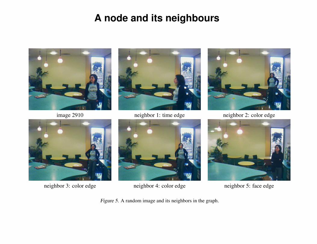
3. The GraphsGraph-based semi-supervised learning depends criticallyon the construction and quality of the graph. The graphshould reflect domain knowledge through the similarityfunction that is used to assign edges (and their weights).For the FreeFoodCam data the nodes in the graph are theimages. An edge is formed between two images accordingto the following criteria:
1. Time edges. People normally move around in thelounge at moderate speed, thus adjacent frames arelikely to contain the same person. We represent thisknowledge in the graph by putting an edge betweentwo images if their time difference is less than athreshold t1 (usually a few seconds).
A node and its neighbours
image 2910 neighbor 1: time edge neighbor 2: color edge
neighbor 3: color edge neighbor 4: color edge neighbor 5: face edge
Figure 5. A random image and its neighbors in the graph.
2. Color edges. The color histogram is largely deter-mined by a person’s apparel. We assume peoplechange clothes on different days, so that the colorhistogram tends to be unusable across multiple days.However, it is an informative feature during a shortertime period (t2), such as half a day. In the graph forevery image i, we find the set of images having a timedifference between (t1, t2) to i, and connect i with itskc-nearest neighbors (in terms of cosine similarity onhistograms) in the set. The parameter kc is a smallinteger, such as three.
3. Face edges. We use face similarity over longer timespans. For every image i with a face, we find the setof images more than t2 apart from i, and connect iwith its kf -nearest neighbor in the set. We use pixel-wise Euclidean distance between face images, wherethe pair of face images is scaled to the same size.
The final graph is the union of the three kinds of edges. Theedges are unweighted. We used t1 = 2 seconds, t2 = 12hours, kc = 3 and kf = 1 below. Conveniently, theseparameters result in a connected graph.
It is impossible to visualize the whole graph. Instead, weshow the neighbors of a random node in Figure 5.
4. AlgorithmsWe use the simple Gaussian field and harmonic functionalgorithm (Zhu et al., 2003) on the FreeFoodCam dataset.
Let l be the number of labeled images, u the number ofunlabeled images, and n = l + u. The graph is representedthe n ! n weight matrixW . Let D be the diagonal degreematrix with Dii =
!j Wij , and define the combinatorial
LaplacianL = D " W (1)
Let Yl be an l!C label matrix, whereC = 10 is the numberof classes. For i = 1 . . . l, Yl(i, c) = 1 if labeled image iis in class c, Yl(i, c) = 0 otherwise. Then the harmonicfunction solution for the unlabeled data is
Yu = "L!1uuLulYl (2)
where Luu is the submatrix of L on unlabeled nodes andso on. Each row of Yu can be interpreted as the collectionof posterior probabilities p(yi = c|Yl) for c = 1 . . . C andi # U . Classification is carried out by finding the class withthe maximal posterior in each row.
In (Zhu et al., 2003) it has also been shown that incor-porating class proportion knowledge can be helpful. Theproportion qc of data with label c can be estimated fromthe labeled set. In particular, the class mass normalization(CMN) heuristic scales the posteriors to meet the propor-tions. That is, one finds a set of coefficients a1, . . . , aC
such that
a1
"
i"U
Yu(i, 1) : · · · : aC
"
i"U
Yu(i, C) = q1 : · · · : qC
(3)
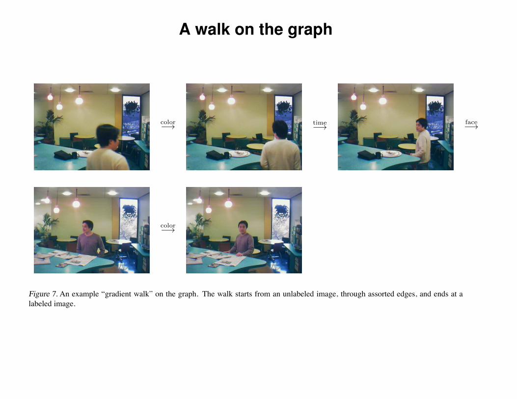
A walk on the graph
color!" time!" face!"
color!"
Figure 7. An example “gradient walk” on the graph. The walk starts from an unlabeled image, through assorted edges, and ends at alabeled image.
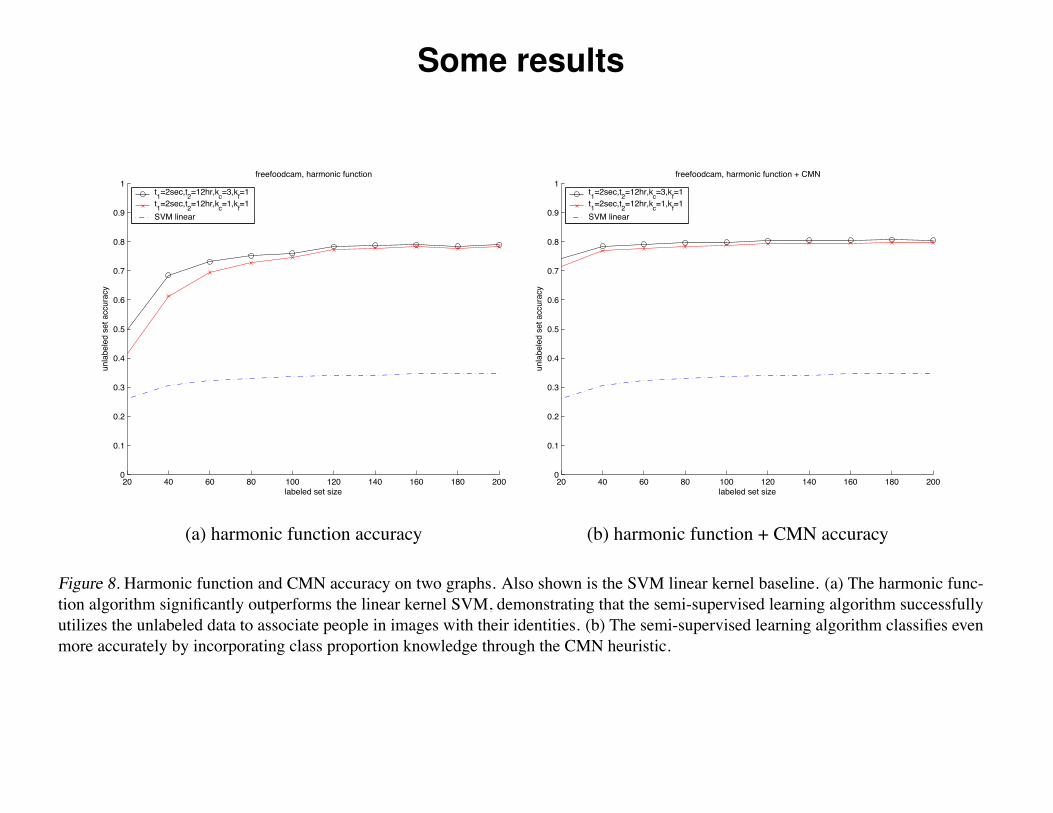
function outperforms the linear kernel SVM baseline (Fig-ure 8). The accuracy can be improved if we incorporateclass proportion knowledge with the simple CMN heuris-tic. The class proportion is estimated from labeled datawith Laplace (add one) smoothing.
To demonstrate the importance of using unlabeled data forsemi-supervised learning, we compare the harmonic func-tion with a minimal unlabeled set of size one. That is,for each unlabeled point xi, we remove all other unlabeledpoints and compute the harmonic function on the labeleddata plus xi. This becomes a supervised learning prob-lem. The harmonic solution with only one unlabeled pointis equivalent to the standard weighted nearest neighbor al-gorithm. Since the original graphs are sparse, most unla-beled points may not have any labeled neighbors. To dealwith this we instead connect xi to its kc nearest labeledneighbors in the color feature, and kf nearest neighbors inthe face feature, where edges are all unweighted. We triedvarious combinations of kc and kf , including those usedin previous experiments. Notice we didn’t use time edge atall, because it does not make sense with only one unlabeledpoint. The results are shown in Figure 9(a) with several dif-ferent setting of kc and kf . The accuracies are all very low.Basically this shows that no combination of color and faceworks if one only use the labeled data. Therefore we seethat using all the unlabeled data is quite important for oursemi-supervised learning approach.
We assigned all the edges equal weights. A natural exten-sion is to give certain types of edges more weight than oth-ers: e.g., perhaps give time-edges more weight than color-
edges. In this case, rather than predicting each example tobe the unweighted average of its neighbors, the predictionbecomes a weighted average. Figure 9(b) shows that bysetting weights judiciously (in particular, giving more em-phasis to time-edges) one can substantially improve perfor-mance, especially on smaller samples. A related problemis to learn the parameters for K-nearest neighbor, i.e. kc
for color edges and kf for face edges. We are currently ex-ploring methods for learning good graph parameter settingsfrom a small set of labeled samples.
6. SummaryIn this paper we formulated a person identification task inlow quality web cam images as a semi-supervised learningproblem, and presented experimental results. The experi-mental setup resembles a video surveillance scenario: lowimage quality and frame rate; labeled data is scarce and isonly available on the first day of a person’s appearance; fa-cial information is not always available in the image. Ourexperiments demonstrate that the semi-supervised learningalgorithms based on harmonic functions are capable of uti-lizing the unlabeled data to identify ten individuals withgreater than 80% accuracy. The dataset is now available tothe research community.
AcknowledgementsWe thank Henry Schneiderman for his help with the facedetector, and Ralph Gross for helpful discussions on im-age processing. We also thank the volunteers for partici-
Some results
20 40 60 80 100 120 140 160 180 2000
0.1
0.2
0.3
0.4
0.5
0.6
0.7
0.8
0.9
1
labeled set size
unla
bele
d se
t acc
urac
y
freefoodcam, harmonic function
t1=2sec,t2=12hr,kc=3,kf=1t1=2sec,t2=12hr,kc=1,kf=1SVM linear
20 40 60 80 100 120 140 160 180 2000
0.1
0.2
0.3
0.4
0.5
0.6
0.7
0.8
0.9
1
labeled set size
unla
bele
d se
t acc
urac
y
freefoodcam, harmonic function + CMN
t1=2sec,t2=12hr,kc=3,kf=1t1=2sec,t2=12hr,kc=1,kf=1SVM linear
(a) harmonic function accuracy (b) harmonic function + CMN accuracy
Figure 8. Harmonic function and CMN accuracy on two graphs. Also shown is the SVM linear kernel baseline. (a) The harmonic func-tion algorithm significantly outperforms the linear kernel SVM, demonstrating that the semi-supervised learning algorithm successfullyutilizes the unlabeled data to associate people in images with their identities. (b) The semi-supervised learning algorithm classifies evenmore accurately by incorporating class proportion knowledge through the CMN heuristic.
pating in the FreeFoodCam dataset collection. This workwas supported in part by the National Science Foundationunder grants CCR-0122581 and IIS-0312814.
ReferencesBlum, A., & Mitchell, T. (1998). Combining labeled andunlabeled data with co-training. COLT: Proceedings ofthe Workshop on Computational Learning Theory.
Gunn, S. R. (1997). Support vector machines for classifi-cation and regression (Technical Report). Image Speechand Intelligent Systems Research Group, University ofSouthampton.
Jain, A. K. (1989). Fundamentals of digital image process-ing. Upper Saddle River, NJ, USA: Prentice-Hall, Inc.
Levin, A., Viola, P. A., & Freund, Y. (2003). Unsupervisedimprovement of visual detectors using co-training. Inter-national Conference on Computer Vision (pp. 626–633).
Nigam, K., McCallum, A. K., Thrun, S., & Mitchell,T. M. (1998). Learning to classify text from labeledand unlabeled documents. AAAI-98, 15th Conference ofthe American Association for Artificial Intelligence (pp.792–799).
Rosenberg, C., Hebert, M., & Schneiderman, H. (2005).Semi-supervised self-training of object detection mod-els. Seventh IEEE Workshop on Applications of Com-puter Vision.
Schneiderman, H. (2004a). Feature-centric evaluation forefficient cascaded object detection. IEEE Conference onComputer Vision and Pattern Recognition (CVPR).
Schneiderman, H. (2004b). Learning a restricted Bayesiannetwork for object detection. IEEE Conference on Com-puter Vision and Pattern Recognition (CVPR).
Schneiderman, H., & Kanade, T. (2002). Object detec-tion using the statistics of parts. International Journalof Computer Vision.
Shin, H., Tsuda, K., & Schlkopf, B. (2004). Protein func-tional class prediction with a combined graph. Proceed-ings of the Korean Data Mining Conference (pp. 200–219).
Weston, J., Leslie, C., Zhou, D., Elisseeff, A., & Noble,W. S. (2004). Semi-supervised protein classification us-ing cluster kernels. Advances in Neural Information Pro-cessing Systems 16.
Zhao, W., Chellappa, R., Phillips, P. J., & Rosenfeld, A.(2003). Face recognition: A literature survey. ACMComputing Surveys, 35, 399–458.
Zhu, X. (2005). Semi-supervised learning with graphs.Doctoral dissertation, Carnegie Mellon University.CMU-LTI-05-192.
Zhu, X., Ghahramani, Z., & Lafferty, J. (2003). Semi-supervised learning using Gaussian fields and harmonicfunctions. ICML-03, 20th International Conference onMachine Learning.
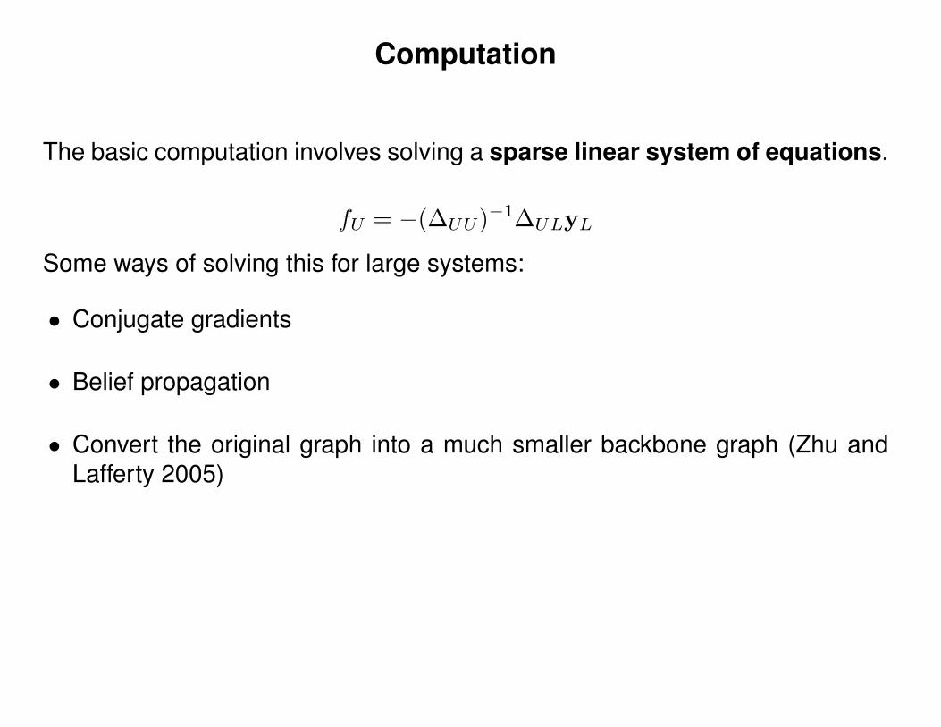
Computation
The basic computation involves solving a sparse linear system of equations.
fU = −(∆UU)−1∆ULyL
Some ways of solving this for large systems:
• Conjugate gradients
• Belief propagation
• Convert the original graph into a much smaller backbone graph (Zhu andLafferty 2005)
Other Approaches to Semi-supervised Learning
Caveat: This is a very big field, a lot has happened since 2003!
• Nigam et al. (2000): An EM algorithm for SSL applied to text.
• Szummer and Jaakkola (2001): SSL using Markov random walks on graphs.
• Belkin and Niyogi (2002): regularize f by using the top few eigenvectors ofthe Laplacian ∆
• Lawrence and Jordan (2005): a Gaussian process approach similar toTSVM using a null category noise model.
• Zhou et al (2004) use the loss function∑i(fi−yi)2 and the normalised graph
Laplacian D−1/2∆D−1/2 as a regulariser.
• Transductive SVMs (also called Semi-Supervised Support Vector Machines(S3VM)).
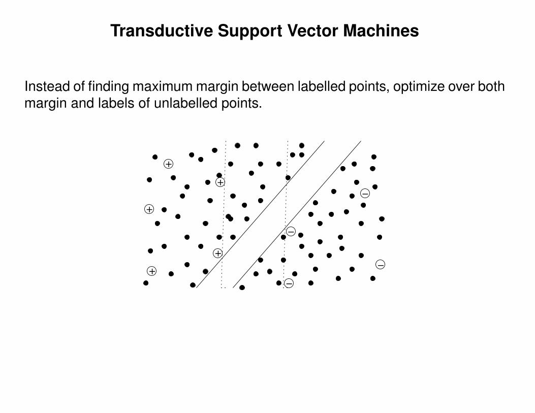
Transductive Support Vector Machines
Instead of finding maximum margin between labelled points, optimize over bothmargin and labels of unlabelled points.
+
+
+
+
+
−
−
−
−
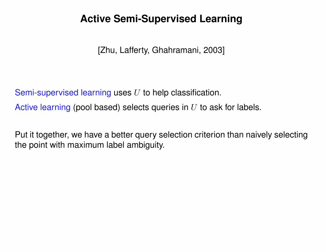
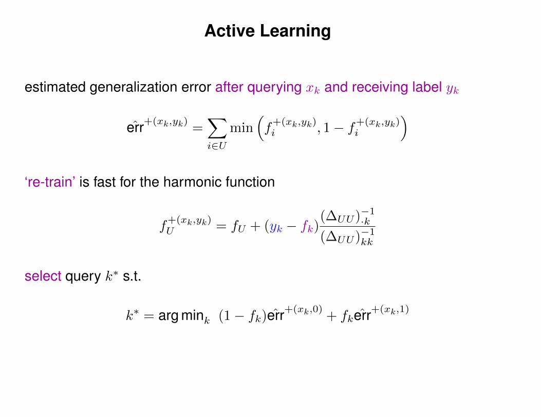
Active Semi-Supervised Learning
[Zhu, Lafferty, Ghahramani, 2003]
Semi-supervised learning uses U to help classification.
Active learning (pool based) selects queries in U to ask for labels.
Put it together, we have a better query selection criterion than naively selectingthe point with maximum label ambiguity.
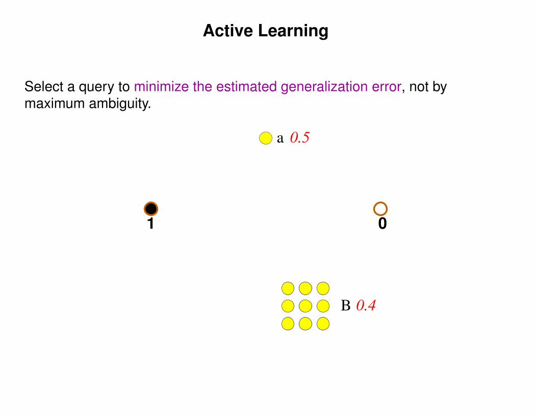
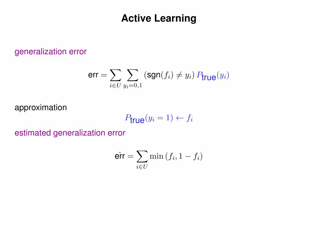
Active Learning
Select a query to minimize the estimated generalization error, not bymaximum ambiguity.
01
a 0.5
B 0.4
Active Learning
generalization error
err =∑
i∈U
∑
yi=0,1
(sgn(fi) 6= yi)Ptrue(yi)
approximationPtrue(yi = 1)← fi
estimated generalization error
err =∑
i∈Umin (fi, 1− fi)
Active Learning
estimated generalization error after querying xk and receiving label yk
err+(xk,yk) =∑
i∈Umin
(f+(xk,yk)i , 1− f+(xk,yk)
i
)
‘re-train’ is fast for the harmonic function
f+(xk,yk)U = fU + (yk − fk)
(∆UU)−1·k(∆UU)−1kk
select query k∗ s.t.
k∗ = arg mink (1− fk)err+(xk,0) + fkerr+(xk,1)
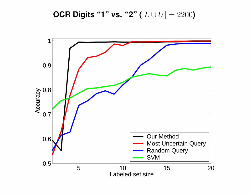
OCR Digits “1” vs. “2” (|L ∪ U | = 2200)
5 10 15 200.5
0.6
0.7
0.8
0.9
1
Labeled set size
Acc
urac
y
Our MethodMost Uncertain QueryRandom QuerySVM
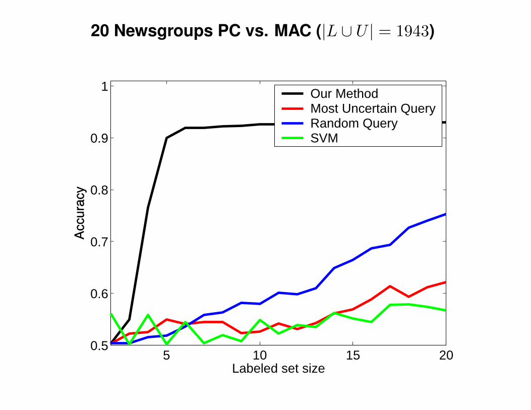
20 Newsgroups PC vs. MAC (|L ∪ U | = 1943)
5 10 15 200.5
0.6
0.7
0.8
0.9
1
Labeled set size
Acc
urac
yOur MethodMost Uncertain QueryRandom QuerySVM
Part II: Some thoughts onBayesian semi-supervised learning
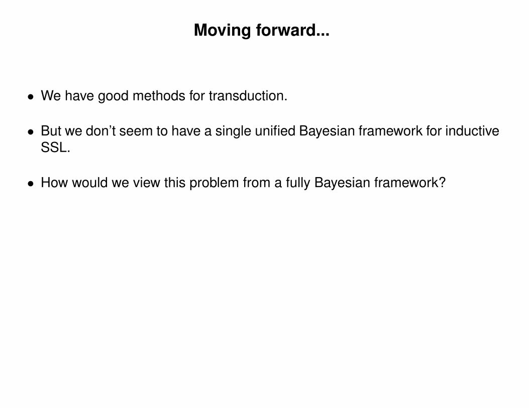
Moving forward...
• We have good methods for transduction.
• But we don’t seem to have a single unified Bayesian framework for inductiveSSL.
• How would we view this problem from a fully Bayesian framework?
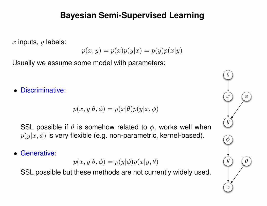
Bayesian Semi-Supervised Learning
x inputs, y labels:p(x, y) = p(x)p(y|x) = p(y)p(x|y)
Usually we assume some model with parameters:
• Discriminative:
p(x, y|θ, φ) = p(x|θ)p(y|x, φ)
SSL possible if θ is somehow related to φ, works well whenp(y|x, φ) is very flexible (e.g. non-parametric, kernel-based).
• Generative:p(x, y|θ, φ) = p(y|φ)p(x|y, θ)
SSL possible but these methods are not currently widely used.
!
!x
y
!
!
x
y
Bayesian Semi-Supervised Learning
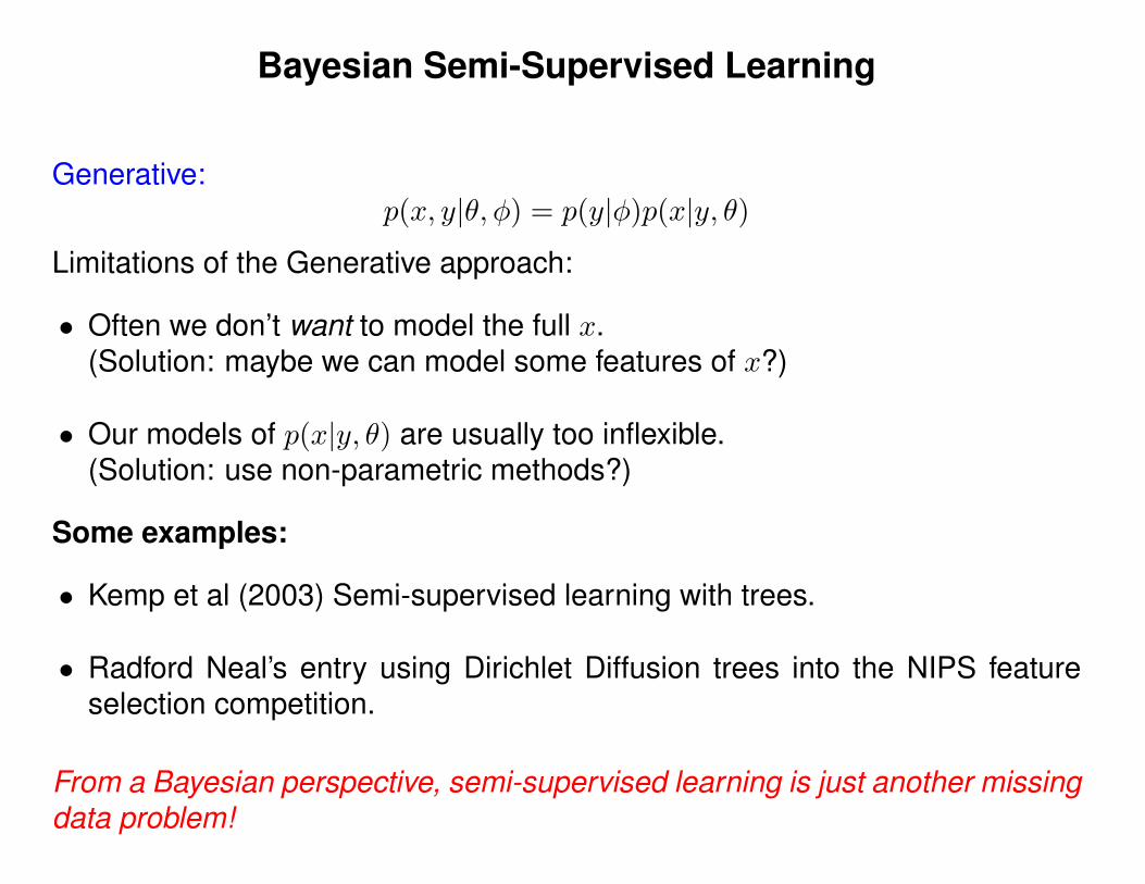
Generative:p(x, y|θ, φ) = p(y|φ)p(x|y, θ)
Limitations of the Generative approach:
• Often we don’t want to model the full x.(Solution: maybe we can model some features of x?)
• Our models of p(x|y, θ) are usually too inflexible.(Solution: use non-parametric methods?)
Some examples:
• Kemp et al (2003) Semi-supervised learning with trees.
• Radford Neal’s entry using Dirichlet Diffusion trees into the NIPS featureselection competition.
From a Bayesian perspective, semi-supervised learning is just another missingdata problem!
Summary
• Semi-supervised learning with harmonic functions
• Active semi-supervised learning using harmonic functions by minimizingexpected generalization error
• Much research in this area but still some open questions...
References
• Balcan, M.-F., Blum, A., Choi, P. P., Lafferty, J., Pantano, B., Rwebangira, M. R., & Zhu, X. (2005a). Personidentification in webcam images: An application of semi-supervised learning. ICML 2005 Workshop onLearning with Partially Classified Training Data.
• Blum, A., & Chawla, S. (2001). Learning from labeled and unlabeled data using graph mincuts. ICML 18.• Joachims, T. (1999). Transductive inference for text classification using support vector machines. ICML 16:
200-209.• Lawrence, N. D., & Jordan, M. I. (2005). Semi-supervised learning via Gaussian processes. NIPS 17.• Nigam, K., McCallum, A. K., Thrun, S., & Mitchell, T. (2000). Text classification from labeled and unlabeled
documents using EM. Machine Learning, 39, 103-134.• Seeger, M. (2001). Learning with labeled and unlabeled data (Technical Report). University of Edinburgh.• Szummer, M., & Jaakkola, T. (2001). Partially labeled classification with Markov random walks. NIPS 14.• Zhou, D., Bousquet, O., Lal, T., Weston, J., & Scholkopf, B. (2004). Learning with local and global consistency.
NIPS 16.• Zhu, X., Ghahramani, Z. and Lafferty, J. (2003) Semi-Supervised Learning Using Gaussian Fields and
Harmonic Functions. ICML 20: 912–919.• Zhu, X., & Lafferty, J. (2005). Harmonic mixtures: combining mixture models and graph-based methods for
inductive and scalable semi-supervised learning. ICML 22.• Zhu, X., Lafferty, J. and Ghahramani, Z. (2003) Combining Active Learning and Semi-Supervised Learning
Using Gaussian Fields and Harmonic Functions. In ICML 2003 Workshop on The Continuum from Labeledto Unlabeled Data in Machine Learning and Data Mining. pp 58–65.
• Zhu, X. and Goldberg, A.B. (2009) Introduction to Semi-Supervised Learning. Morgan-Claypool.