Embed Size (px)
Citation preview

The Modelling of Granular Flow Using theParticle-in-Cell Method
by
Corné J Coetzee
Dissertation approved for the degree of Doctor of Philosophy inMechanical Engineering at Stellenbosch University
Department of Mechanical Engineering,University of Stellenbosch,
Private Bag X1, Matieland 7602, South Africa.
Promoters:
Prof A.H. BassonMechanical EngineeringUniversity of Stellenbosch
Prof P.A. VermeerInstitut für GeotechnicUniversität Stuttgart
April 2004

Copyright ©2004 University of StellenboschAll rights reserved.

Declaration
I, the undersigned, hereby declare that the work contained in this disserta-tion is my own original work and that I have not previously in its entiretyor in part submitted it at any university for a degree.
Signature: . . . . . . . . . . . . . . . . . . . . . . . . . .CJ Coetzee
Date: . . . . . . . . . . . . . . . . . . . . . . . . . . . . . . .
ii

Abstract
The Modelling of Granular Flow Using the Particle-in-Cell Method
CJ Coetzee
Granular flow occurs in a broad spectrum of industrial applications thatrange from separation and mixing in the pharmaceutical industry, to grin-ding and crushing, blasting, stockpile construction, flow in and from hop-pers, silos, bins, and conveyer belts, agriculture, mining and earthmoving.
Two totally different approaches of modelling granular flow are the Dis-crete Element Method (DEM) and continuum methods such as Finite Ele-ment Methods (FEM). Continuum methods can be divided into nonpolar orclassic continuum methods and polar continuum methods. Large displace-ments are usually present during granular flow which, without remeshing,cannot be solved with standard finite element methods due to severe meshdistortion. The Particle-in-Cell (PIC) method, which is a so-called meshlessmethod, eliminates this problem since all the state variables are traced bymaterial points moving through a fixed mesh.
The main goal of this research was to model the flow of noncohesivegranular material in front of flat bulldozer blades and into excavator bucketsusing a continuum method. A PIC code was developed to model these pro-cesses under plane strain conditions. A contact model was used to modelCoulomb friction between the material and the bucket/blade. Analyticalsolutions, published numerical and experimental results were used to vali-date the contact model and to demonstrate the code’s ability to model largedisplacements and deformations.
The ability of both DEM and PIC to predict the forces acting on the bladeand bucket and the material flow patterns were demonstrated. Shear bandsthat develop during the flow of material were investigated. As part of thePIC analyses, a comparison between classic continuum and polar conti-nuum (Cosserat) results were made. This includes mesh size and orien-tation dependency, flow patterns and the forces acting on the blade and thebucket.
It is concluded that the interaction of buckets and blades with granu-lar materials can successfully be modelled with PIC. In the cases conduc-ted here, the nonpolar continuum was more accurate than the polar conti-nuum, but the polar continuum results were less dependent on the meshsize. The next step would be to apply this technology to solve industrialproblems.
Keywords: Granular flow; Particle-in-Cell method; Discrete Element Me-thod; Bucket filling; Silo discharging
iii

Uittreksel
The Modelling of Granular Flow Using the Particle-in-Cell Method
CJ Coetzee
Partikelvloei kom voor in ’n verskeidenheid industriële toepassings vanafskeiding en mengprosesse in die farmaseutiese industrie tot vergruising,die vloei in vulbakke en silos, vervoerbande, landboubewerkings, myn-wese en grondverskuiwing.
Twee verskillende metodes om partikelvloei te modelleer kan onders-kei word, naamlik Diskrete Element Metodes (DEM) en kontinuum meto-des soos Eindige Element Metodes. Kontinuum metodes kan verdeel wordin nie-polêre of klassieke kontinuum metodes en polêre kontinuum me-todes. Groot verplasings is gewoontlik teenwoordig tydens partikelvloeiwat dit moeilik maak om dit met behulp van Eindige Element Metodesop te los weens groot vervorming van die elemente. Die "Particle-in-Cell"(PIC) metode is ’n sogenaamde roosterlose metode wat hierdie probleemelimineer aangesien al die toestandsveranderlikes gekoppel is aan mate-riaalpunte wat deur die vaste rooster beweeg.
Die hoofdoel van die navorsing was om die partikelvloei van kohesie-lose materiale soos veroorsaak deur ’n plat lem en ’n masjiengraaf laaibakte modelleer deur van ’n kontinuum metode gebruik te maak. ’n PIC kodeis ontwikkel om dié prosesse onder die aanname van vlakspanning the mo-delleer. ’n Kontakmodel is gebruik om Coulomb wrywing tussen die mate-riaal en die bak/lem te modelleer. Analitiese oplossings en gepubliseerdenumeriese en eksperimentele resultate is gebruik om die kontakmodel endie vermoë van die kode om groot verplasings en vervormings te model-leer, te valideer.
Die mate waarin DEM en PIC die kragte wat op die lem en bak uitgeo-efen word en die vloeipatrone, kan voorspel, word gedemonstreer. Glip-vlakke wat gedurende die vloei van materiaal ontstaan is ondersoek. Asdeel van die PIC analises, is die nie-polêre en polêre (Cosserat) kontinuamet mekaar vergelyk. Dit sluit in roostergrootte en oriëntasie onafhanklik-heid, vloeipatrone en die kragte wat op die lem en bak inwerk.
Die gevolgtreking word gemaak dat die interaksie van bakke en lemmemet ’n korrelrige materiaal suksesvol met behulp van PIC gemodelleer kanword. In die gevalle hier getoets, was die nie-polêre kontinuum meer ak-kuraat as die polêre kontinuum, maar die nie-polêre kontinuum resultateminder afhanklik van die roostergrootte. Die volgende stap sou wees omhierdie tegnologie in die industrie toe te pas.
iv

Contents
Declaration ii
Abstract iii
Uittreksel iv
Contents v
List of Figures x
List of Tables xvi
Nomenclature xvii
Chapter 1 An Introduction: Modelling of Granular Flow 11.1 Introduction . . . . . . . . . . . . . . . . . . . . . . . . . . . . 11.2 Theories for Modelling Granular Materials . . . . . . . . . . 2
1.2.1 Discrete Element Methods . . . . . . . . . . . . . . . . 21.2.2 Continuum Theory . . . . . . . . . . . . . . . . . . . . 3
1.3 Numerical Methods . . . . . . . . . . . . . . . . . . . . . . . . 81.3.1 The Finite Element Method . . . . . . . . . . . . . . . 81.3.2 Meshless Methods . . . . . . . . . . . . . . . . . . . . 101.3.3 The Particle-in-Cell Method . . . . . . . . . . . . . . . 10
1.4 Thesis Goals and Outline . . . . . . . . . . . . . . . . . . . . . 121.4.1 Goals . . . . . . . . . . . . . . . . . . . . . . . . . . . . 121.4.2 Novelty . . . . . . . . . . . . . . . . . . . . . . . . . . 141.4.3 Outline . . . . . . . . . . . . . . . . . . . . . . . . . . . 14
Chapter 2 Governing Equations 162.1 Introduction . . . . . . . . . . . . . . . . . . . . . . . . . . . . 162.2 Space Discretisation . . . . . . . . . . . . . . . . . . . . . . . . 162.3 Element Formulation . . . . . . . . . . . . . . . . . . . . . . . 182.4 Time Integration . . . . . . . . . . . . . . . . . . . . . . . . . . 20
2.4.1 Initialisation phase . . . . . . . . . . . . . . . . . . . . 202.4.2 Lagrangian phase . . . . . . . . . . . . . . . . . . . . . 202.4.3 Convective phase . . . . . . . . . . . . . . . . . . . . . 21
2.5 Stability . . . . . . . . . . . . . . . . . . . . . . . . . . . . . . . 222.6 The Polar Continuum . . . . . . . . . . . . . . . . . . . . . . . 222.7 Constitutive Models . . . . . . . . . . . . . . . . . . . . . . . 23
v

Contents vi
Chapter 3 Boundary and Initial Conditions 283.1 Introduction . . . . . . . . . . . . . . . . . . . . . . . . . . . . 283.2 Boundary Conditions . . . . . . . . . . . . . . . . . . . . . . . 283.3 Initial Conditions and Damping . . . . . . . . . . . . . . . . . 29
3.3.1 Uniform Stress Field . . . . . . . . . . . . . . . . . . . 293.3.2 Stress Field with a Gradient . . . . . . . . . . . . . . . 293.3.3 Layer-by-Layer Method . . . . . . . . . . . . . . . . . 30
Chapter 4 Numerical and Analytical Validation 324.1 Introduction . . . . . . . . . . . . . . . . . . . . . . . . . . . . 324.2 Simulation of a High Velocity Impact . . . . . . . . . . . . . . 324.3 Inclined Plane Simulation . . . . . . . . . . . . . . . . . . . . 394.4 Impact of Two Elastic Bodies . . . . . . . . . . . . . . . . . . 424.5 Oedometer Test . . . . . . . . . . . . . . . . . . . . . . . . . . 504.6 Silo Discharging . . . . . . . . . . . . . . . . . . . . . . . . . . 544.7 Blade Simulations . . . . . . . . . . . . . . . . . . . . . . . . . 594.8 Elastic Strip Footing . . . . . . . . . . . . . . . . . . . . . . . . 68
Chapter 5 Experimental Validation 715.1 Introduction . . . . . . . . . . . . . . . . . . . . . . . . . . . . 715.2 Anchor Plates in Sand . . . . . . . . . . . . . . . . . . . . . . 71
5.2.1 Vertically Pulled Anchors . . . . . . . . . . . . . . . . 715.2.2 Anchor Pulled at 45° . . . . . . . . . . . . . . . . . . . 75
5.3 Strip Footings . . . . . . . . . . . . . . . . . . . . . . . . . . . 815.3.1 Test Setup . . . . . . . . . . . . . . . . . . . . . . . . . 815.3.2 Soil Parameters . . . . . . . . . . . . . . . . . . . . . . 825.3.3 Bearing Capacity . . . . . . . . . . . . . . . . . . . . . 845.3.4 Slope Stability . . . . . . . . . . . . . . . . . . . . . . . 865.3.5 Conclusions . . . . . . . . . . . . . . . . . . . . . . . . 88
Chapter 6 Blade, Bucket and Silo Modelling 906.1 Introduction . . . . . . . . . . . . . . . . . . . . . . . . . . . . 906.2 Blade and Bucket Modelling . . . . . . . . . . . . . . . . . . . 90
6.2.1 Two-dimensional Test Rig . . . . . . . . . . . . . . . . 906.2.2 Material . . . . . . . . . . . . . . . . . . . . . . . . . . 926.2.3 DEM Simulations . . . . . . . . . . . . . . . . . . . . . 946.2.4 Effect of Tool Velocity . . . . . . . . . . . . . . . . . . 956.2.5 Vertical Blade Modelling . . . . . . . . . . . . . . . . . 966.2.6 Bucket Modelling . . . . . . . . . . . . . . . . . . . . . 117
6.3 Silo Modelling . . . . . . . . . . . . . . . . . . . . . . . . . . . 1316.4 Computing Times . . . . . . . . . . . . . . . . . . . . . . . . . 139
Chapter 7 Concluding Remarks and Recommendations 141

Contents vii
Appendix A Notation and Basic Principles 145A.1 Introduction . . . . . . . . . . . . . . . . . . . . . . . . . . . . 145A.2 Index Notation . . . . . . . . . . . . . . . . . . . . . . . . . . 145
A.2.1 Index Notation of a Vector . . . . . . . . . . . . . . . . 145A.2.2 Transformation Law of a Vector . . . . . . . . . . . . . 146A.2.3 Rules of the Index Notation and Transformation Laws 147A.2.4 Addition and Subtraction of Vectors and Cartesian
Tensors . . . . . . . . . . . . . . . . . . . . . . . . . . 150A.2.5 Scalar or Dot Product . . . . . . . . . . . . . . . . . . 150A.2.6 Vector or Cross Product . . . . . . . . . . . . . . . . . 150A.2.7 Multiplication of Cartesian Tensors . . . . . . . . . . 151
A.3 Matrix Tensor Notation . . . . . . . . . . . . . . . . . . . . . . 152A.3.1 Vector . . . . . . . . . . . . . . . . . . . . . . . . . . . 152A.3.2 Matrix . . . . . . . . . . . . . . . . . . . . . . . . . . . 152A.3.3 Multiplication Rules . . . . . . . . . . . . . . . . . . . 152A.3.4 Scalar Product . . . . . . . . . . . . . . . . . . . . . . . 153A.3.5 Norm . . . . . . . . . . . . . . . . . . . . . . . . . . . . 153A.3.6 Physical Vectors . . . . . . . . . . . . . . . . . . . . . . 153A.3.7 Base . . . . . . . . . . . . . . . . . . . . . . . . . . . . 154A.3.8 Transformations . . . . . . . . . . . . . . . . . . . . . 155A.3.9 Vector or Cross Product . . . . . . . . . . . . . . . . . 156A.3.10 Rotating Base . . . . . . . . . . . . . . . . . . . . . . . 157
A.4 Combined Notation . . . . . . . . . . . . . . . . . . . . . . . . 157A.5 General Principles . . . . . . . . . . . . . . . . . . . . . . . . . 157
A.5.1 Gradient of a Scalar Function . . . . . . . . . . . . . . 157A.5.2 Divergence of a Vector Function . . . . . . . . . . . . 158A.5.3 Curl of a Vector Function . . . . . . . . . . . . . . . . 158A.5.4 Gauss’ Theorem . . . . . . . . . . . . . . . . . . . . . . 158A.5.5 Lagrangian and Eulerian Descriptions of Deforma-
tion or Flow . . . . . . . . . . . . . . . . . . . . . . . . 159A.5.6 The Comoving Derivative . . . . . . . . . . . . . . . . 161A.5.7 The Reynolds Transport Theorem . . . . . . . . . . . 162
Appendix B Nonpolar Continuum Mechanics 165B.1 Introduction . . . . . . . . . . . . . . . . . . . . . . . . . . . . 165B.2 Cauchy Stress Tensor . . . . . . . . . . . . . . . . . . . . . . . 165B.3 Principal Stresses and Principal Axes . . . . . . . . . . . . . . 169B.4 Conservation of Mass . . . . . . . . . . . . . . . . . . . . . . . 170
B.4.1 Eulerian Description . . . . . . . . . . . . . . . . . . . 170B.4.2 Lagrangian Description . . . . . . . . . . . . . . . . . 172
B.5 Momentum Balance Principles . . . . . . . . . . . . . . . . . 175B.5.1 Eulerian Description . . . . . . . . . . . . . . . . . . . 175B.5.2 Lagrangian Description . . . . . . . . . . . . . . . . . 178
B.6 Strain Tensor . . . . . . . . . . . . . . . . . . . . . . . . . . . . 179

Contents viii
B.6.1 General or Finite Strain . . . . . . . . . . . . . . . . . 179B.6.2 Infinitesimal Strain . . . . . . . . . . . . . . . . . . . . 182B.6.3 The Linear Rotation Tensor and Rotation Vector . . . 184B.6.4 Geometrical Meanings of the Linear Strain Tensors . 187
B.7 Principal Strains and Principal Axes . . . . . . . . . . . . . . 189B.8 The Linear Cubical Dilatation . . . . . . . . . . . . . . . . . . 191B.9 Compatibility Equations for Linear Strain Components . . . 192
B.9.1 Eulerian Description . . . . . . . . . . . . . . . . . . . 192B.9.2 Lagrangian Description . . . . . . . . . . . . . . . . . 195
B.10 The Rate of Strain Tensor and the Vorticity Tensor . . . . . . 195B.11 The Rate of Rotation Vector and the Vorticity Vector . . . . . 197
Appendix C Polar Continuum Mechanics 199C.1 Introduction . . . . . . . . . . . . . . . . . . . . . . . . . . . . 199C.2 The Cosserat Equations . . . . . . . . . . . . . . . . . . . . . . 199
C.2.1 The Couple-Stress Tensor and Couple-Stress Vector . 199C.2.2 Momentum Balance Principles . . . . . . . . . . . . . 204C.2.3 Mohr’s Circle of Non-Symmetric Stress Tensor . . . . 207
C.3 Kinematics of Cosserat Continua . . . . . . . . . . . . . . . . 210
Appendix D Rigid Body Motion 215D.1 Introduction . . . . . . . . . . . . . . . . . . . . . . . . . . . . 215D.2 Kinematic Relations . . . . . . . . . . . . . . . . . . . . . . . . 215D.3 Linear and Angular Momentum of a Rigid Body . . . . . . . 217
Appendix E The Finite Element Method 220E.1 Introduction . . . . . . . . . . . . . . . . . . . . . . . . . . . . 220E.2 Plane Bilinear Isoparametric Element . . . . . . . . . . . . . . 220
E.2.1 Stiffness Matrix Formulation . . . . . . . . . . . . . . 220E.2.2 Load Vector Formulation . . . . . . . . . . . . . . . . 224
E.3 Summary of Gauss Quadrature . . . . . . . . . . . . . . . . . 226E.3.1 One Dimension . . . . . . . . . . . . . . . . . . . . . . 226E.3.2 Two Dimensions . . . . . . . . . . . . . . . . . . . . . 227
Appendix F The Particle-in-Cell Method Based on the Cosserat Con-tinuum 230
F.1 Introduction . . . . . . . . . . . . . . . . . . . . . . . . . . . . 230F.2 PIC Mass Representation . . . . . . . . . . . . . . . . . . . . . 230F.3 The Cosserat Governing Equations . . . . . . . . . . . . . . . 233F.4 The Weak Form of the Governing Equations . . . . . . . . . 233F.5 The Finite Element Representation . . . . . . . . . . . . . . . 235F.6 Numerical Algorithm . . . . . . . . . . . . . . . . . . . . . . . 251
F.6.1 Initialisation Phase . . . . . . . . . . . . . . . . . . . . 251F.6.2 Lagrangian Phase . . . . . . . . . . . . . . . . . . . . . 253

Contents ix
F.6.3 Convective Phase . . . . . . . . . . . . . . . . . . . . . 257F.7 Numerical Implementation . . . . . . . . . . . . . . . . . . . 258F.8 Numerical Algorithm . . . . . . . . . . . . . . . . . . . . . . . 261F.9 Numerical Integration: Convergence and Stability . . . . . . 265F.10 Damping . . . . . . . . . . . . . . . . . . . . . . . . . . . . . . 266
Appendix G Particle-in-Cell Contact Model 270G.1 Introduction . . . . . . . . . . . . . . . . . . . . . . . . . . . . 270G.2 Contact Model . . . . . . . . . . . . . . . . . . . . . . . . . . . 270G.3 Boundary Unit Normal Vector Calculation . . . . . . . . . . 276G.4 Implementation . . . . . . . . . . . . . . . . . . . . . . . . . . 282
Appendix H Nonpolar Constitutive Models and Implementation 284H.1 Introduction . . . . . . . . . . . . . . . . . . . . . . . . . . . . 284H.2 Elastic, Isotropic Model . . . . . . . . . . . . . . . . . . . . . . 284
H.2.1 Plane Strain . . . . . . . . . . . . . . . . . . . . . . . . 284H.2.2 Plane Stress . . . . . . . . . . . . . . . . . . . . . . . . 285
H.3 Drucker-Prager Model . . . . . . . . . . . . . . . . . . . . . . 285H.3.1 Incremental Elastic Law . . . . . . . . . . . . . . . . . 285H.3.2 Yield and Potential Functions . . . . . . . . . . . . . . 286H.3.3 Plastic Corrections . . . . . . . . . . . . . . . . . . . . 288H.3.4 Implementation Procedure . . . . . . . . . . . . . . . 291
H.4 The von Mises Model . . . . . . . . . . . . . . . . . . . . . . . 292H.4.1 Plastic Corrections . . . . . . . . . . . . . . . . . . . . 293H.4.2 Implementation Procedure . . . . . . . . . . . . . . . 294
H.5 The Mohr-Coulomb Model . . . . . . . . . . . . . . . . . . . 295H.5.1 Plastic Corrections . . . . . . . . . . . . . . . . . . . . 298H.5.2 Implementation Procedure . . . . . . . . . . . . . . . 300H.5.3 Strain-Hardening and -Softening . . . . . . . . . . . . 302H.5.4 Oedometer Test . . . . . . . . . . . . . . . . . . . . . . 304
H.6 The Relation Between the Different Constitutive Models . . 307
Appendix I Cosserat Continuum Constitutive Models and Imple-mentation 309
I.1 Introduction . . . . . . . . . . . . . . . . . . . . . . . . . . . . 309I.2 Cosserat Plane Strain Elasticity . . . . . . . . . . . . . . . . . 309I.3 Cosserat von Mises Elasto-Plasticity . . . . . . . . . . . . . . 312
I.3.1 Algorithm . . . . . . . . . . . . . . . . . . . . . . . . . 315I.4 Generalisation of J2-flow Theory . . . . . . . . . . . . . . . . 317
I.4.1 A Return-mapping Algorithm . . . . . . . . . . . . . 320I.5 Cosserat Drucker-Prager Elasto-Plasticity . . . . . . . . . . . 322
References 325

List of Figures
1.1 A typical walking dragline . . . . . . . . . . . . . . . . . . . . . 13
2.1 The element mesh and material points within the subdomains 17
3.1 Layer-by-layer method of generating initial stresses . . . . . . 31
4.1 Penetrated configuration at t = 24 µs, (Sulsky and Schreyer,1993) . . . . . . . . . . . . . . . . . . . . . . . . . . . . . . . . . 33
4.2 Penetrated configuration at t = 24 µs, (PICCUS) . . . . . . . . . 344.3 Depth of penetration as a function of time . . . . . . . . . . . . 354.4 Penetration at t = 0 µs, particles configuration and von Mises
stress . . . . . . . . . . . . . . . . . . . . . . . . . . . . . . . . . 364.5 Penetration at t = 3.2 µs, particles configuration and von Mi-
ses stress . . . . . . . . . . . . . . . . . . . . . . . . . . . . . . . 364.6 Penetration at t = 6.4 µs, particles configuration and von Mi-
ses stress . . . . . . . . . . . . . . . . . . . . . . . . . . . . . . . 374.7 Penetration at t = 9.6 µs, particles configuration and von Mi-
ses stress . . . . . . . . . . . . . . . . . . . . . . . . . . . . . . . 374.8 Penetration at t = 12.8 µs, particles configuration and von Mi-
ses stress . . . . . . . . . . . . . . . . . . . . . . . . . . . . . . . 384.9 Penetration at t = 32 µs, particles configuration and von Mises
stress . . . . . . . . . . . . . . . . . . . . . . . . . . . . . . . . . 384.10 Penetration at t = 80 µs, particles configuration and von Mises
stress . . . . . . . . . . . . . . . . . . . . . . . . . . . . . . . . . 394.11 (a) Cylinder on an inclined plane, (b) Geometry for simulation
of cylinder on inclined plane . . . . . . . . . . . . . . . . . . . . 40
4.12 Disk at time t = 0.3 s, θ = 60, µ = 0.9. Velocity vectors V−→10 . . 41
4.13 Inclined plane simulation: Centre position for different inclineangles, friction coefficients and mesh sizes . . . . . . . . . . . . 42
4.14 Initial positions of the disks at time t = 0.00 s . . . . . . . . . . 434.15 Positions of the disks at the point of contact, t = 1.30 s . . . . . 434.16 Positions of the disks at the point of minimum kinetic energy,
t = 1.96 s . . . . . . . . . . . . . . . . . . . . . . . . . . . . . . . 444.17 Positions of the disks at the point where contact is broken, t =
2.68 s . . . . . . . . . . . . . . . . . . . . . . . . . . . . . . . . . 454.18 Momentum as a function of time for the disk starting in the
upper left hand corner, ∆t = 1× 10⁻⁵ s . . . . . . . . . . . . . . 454.19 Energy as a function of time, ∆t = 1× 10⁻⁵ s. No slip contact . 464.20 Gain/Dissipation in total energy as a percentage of the total
energy at t = 0. Gain being positive and dissipation negative.No slip contact . . . . . . . . . . . . . . . . . . . . . . . . . . . . 47
x

List of Figures xi
4.21 Energy as a function of time, ∆t = 1× 10⁻⁵ s, µ = 0.1 . . . . . 494.22 Gain/Dissipation in total energy as a percentage of the total
energy at t = 0. Gain being positive and dissipation negative,∆t = 1× 10⁻⁵ s . . . . . . . . . . . . . . . . . . . . . . . . . . . 50
4.23 Boundary conditions for oedometer test (FLAC, 1998) . . . . . 514.24 Oedometer test: Simulation setup with 9 particles per element.
Plunger material point velocity vectors v−→100 . . . . . . . . . . . 52
4.25 Oedometer test: Comparison between numerical and analyti-cal predictions . . . . . . . . . . . . . . . . . . . . . . . . . . . . 53
4.26 Oedometer test: Rigid body (plunger) force and normal stress(absolute values) . . . . . . . . . . . . . . . . . . . . . . . . . . 54
4.27 Silo shape. Dimensions in mm . . . . . . . . . . . . . . . . . . . 554.28 Material stresses at equilibrium . . . . . . . . . . . . . . . . . . 564.29 Deformations at time 0.2 and 0.4 seconds, Wieckowski (1998) . 574.30 Deformations at time 0.2 and 0.4 seconds, PICCUS . . . . . . . 574.31 Silo flow rate . . . . . . . . . . . . . . . . . . . . . . . . . . . . . 584.32 Blade forces - sample calculation . . . . . . . . . . . . . . . . . 604.33 Initial particle configuration close to the blade, h = 0.27 m . . . 604.34 Blade simulation: initial stresses, h = 0.27 m . . . . . . . . . . . 624.35 Blade simulation: typical blade forces, h = 0.21 m . . . . . . . 634.36 Blade simulation: Comparison of blade forces . . . . . . . . . . 644.37 Blade simulation: Percentage difference in the prediction of
the blade forces . . . . . . . . . . . . . . . . . . . . . . . . . . . 654.38 Blade simulation: Particle velocity vectors, scaled 15 times,
h = 0.27 m . . . . . . . . . . . . . . . . . . . . . . . . . . . . . . 654.39 Blade simulation: Material stress, lighter regions - material
yielding, darker regions - material in an elastic state, h = 0.27 m 664.40 Blade simulation: Material stress, lighter regions - material
yielding, darker regions - material in an elastic state, h = 0.15 m 664.41 The effect of the mesh size on the blade forces, h = 0.21 m . . . 674.42 PICCUS model for strip loading on an elastic mass . . . . . . . 684.43 Definition of parameters used in the elastic solution to the foo-
ting problem . . . . . . . . . . . . . . . . . . . . . . . . . . . . . 694.44 Comparison of stresses σ1 and σ3 along x1 = 0 under the strip
footing . . . . . . . . . . . . . . . . . . . . . . . . . . . . . . . . 70
5.1 Geometry for vertically pulled anchor. Dimensions are in mm. 725.2 Simulation model for vertically pulled anchor. . . . . . . . . . 735.3 Load-displacement curve for vertically pulled anchor, h
B = 3. . 755.4 Load-displacement curve for vertically pulled anchor, h
B = 5. . 765.5 Comparison between Mohr-Coulomb and Drucker-Prager mo-
dels on vertically pulled anchor, hB = 3, smooth interface, E =
1000 kN·m−2 . . . . . . . . . . . . . . . . . . . . . . . . . . . . . 775.6 Geometry for anchor pulled at 45. Dimensions are in mm. . . 77

List of Figures xii
5.7 Computed Geometry for anchor pulled at 45. . . . . . . . . . 785.8 Load-displacement curve for anchor pulled at 45°, h
B = 2. . . . 795.9 The ultimate capacity at different depth ratios for the anchor
pulled at 45°. . . . . . . . . . . . . . . . . . . . . . . . . . . . . . 805.10 Test setup, Rilling (1994). Dimensions in cm . . . . . . . . . . . 825.11 Load-displacement curves from field tests. . . . . . . . . . . . 835.12 Triaxial results for Heilbronn silt . . . . . . . . . . . . . . . . . 845.13 Discretisation of the bearing capacity problem: (a) PLAXIS and
(b) PICCUS (not to the same scale). Dimensions in m . . . . . . 855.14 Load-displacement curves for bearing capacity . . . . . . . . . 865.15 Discretisation of the slope stability problem: (a) PLAXIS and
(b) PICCUS. Dimensions in m . . . . . . . . . . . . . . . . . . . 875.16 Load-displacement curves for slope stability . . . . . . . . . . 88
6.1 Two-dimensional test rig, Coetzee (2000) . . . . . . . . . . . . . 916.2 2-D Test rig arm mechanism, Coetzee (2000) . . . . . . . . . . . 926.3 Bucket dimensions in mm . . . . . . . . . . . . . . . . . . . . . 936.4 Corn grains, Coetzee (2000) . . . . . . . . . . . . . . . . . . . . 936.5 Corn grains (a) measured [mm] (b) DEM grain, Coetzee (2000) 946.6 Stresses at equilibrium . . . . . . . . . . . . . . . . . . . . . . . 976.7 Comparison between experimental, DEM and nonpolar results
of corn flowing in front of the blade, displacement = 100 mmand 200 mm . . . . . . . . . . . . . . . . . . . . . . . . . . . . . 98
6.8 Comparison between experimental, DEM and nonpolar resultsof corn flowing in front of the blade, displacement = 300 mmand 400 mm . . . . . . . . . . . . . . . . . . . . . . . . . . . . . 99
6.9 Comparison of the free surfaces using different dilatancy angles 1006.10 Comparison between polar and nonpolar results of corn flo-
wing in front of the blade, ψ = 2 . . . . . . . . . . . . . . . . . 1016.11 Comparison of the experimental, polar (ψ = 2), nonpolar
(ψ = 2) and DEM free surfaces . . . . . . . . . . . . . . . . . . 1026.12 The effect of the dilatancy angle ψ on the blade forces, h =
350 mm . . . . . . . . . . . . . . . . . . . . . . . . . . . . . . . . 1036.13 The effect blade depth h on the blade forces using a nonpolar
continuum and ψ = 2 . . . . . . . . . . . . . . . . . . . . . . . 1046.14 Comparison between average draft fores: PICCUS, DEM, expe-
riments and Sokolovski’s method . . . . . . . . . . . . . . . . . 1056.15 Predicted shear bands using a particle displacement ratio PDR
= 0.15, x1 = 15 mm . . . . . . . . . . . . . . . . . . . . . . . . . 1066.16 Nonpolar yield points: mesh sizes 120× 70 and 80× 50, x1 =
15 mm . . . . . . . . . . . . . . . . . . . . . . . . . . . . . . . . . 1086.17 Nonpolar shear strains for mesh sizes 120 × 70 and 80 × 50,
x1 = 15 mm . . . . . . . . . . . . . . . . . . . . . . . . . . . . . 109

List of Figures xiii
6.18 Polar rotations [rad] for mesh sizes 120× 70 and 80× 50, x1 =15 mm . . . . . . . . . . . . . . . . . . . . . . . . . . . . . . . . . 110
6.19 Nonpolar shear strain and polar rotation using a 80× 50 meshrotated through 35 , x1 = 15 mm . . . . . . . . . . . . . . . . . 111
6.20 The velocity fields in front of the blade, x1 = 15 mm . . . . . . 1126.21 Normal and shear stress at the blade for h = 350 mm: Nonpo-
lar continuum and Sokolovski’s method, x1 = 20 mm . . . . . 1146.22 Normal and shear stress at the blade for h = 350 mm: Polar
continuum, with and without rotation at the blade, and Soko-lovski’s method, x1 = 20 mm . . . . . . . . . . . . . . . . . . . 115
6.23 Force chains at the blade for h = 350 mm, x1 = 20 mm . . . . . 1156.24 Normal and shear pressures at the blade for h = 350 mm: DEM
and Sokolovski’s method . . . . . . . . . . . . . . . . . . . . . . 1166.25 Bucket draft force as measured and predicted by the nonpolar
continuum, polar continuum and DEM . . . . . . . . . . . . . . 1186.26 The flow of corn into the bucket: displacement = 100 mm -
200 mm . . . . . . . . . . . . . . . . . . . . . . . . . . . . . . . . 1196.27 The flow of corn into the bucket: displacement = 300 mm -
400 mm . . . . . . . . . . . . . . . . . . . . . . . . . . . . . . . . 1206.28 The flow of corn into the bucket: displacement = 500 mm -
600 mm . . . . . . . . . . . . . . . . . . . . . . . . . . . . . . . . 1216.29 The flow of corn into the bucket: displacement = 700 mm -
800 mm . . . . . . . . . . . . . . . . . . . . . . . . . . . . . . . . 1226.30 Comparison of the free surface of the material flowing into the
bucket . . . . . . . . . . . . . . . . . . . . . . . . . . . . . . . . . 1236.31 The Shear Zone Theory developed by Rowlands (1991) . . . . 1256.32 The Shear Zone Theory at a displacement of 100 mm . . . . . . 1276.33 The Shear Zone Theory at a displacement of 500 mm . . . . . . 1286.34 The Shear Zone Theory at a displacement of 800 mm . . . . . . 1296.35 The normal stress on the inside of the bucket at a displacement
of 800 mm . . . . . . . . . . . . . . . . . . . . . . . . . . . . . . 1306.36 The shear stress on the inside of the bucket at a displacement
of 800 mm . . . . . . . . . . . . . . . . . . . . . . . . . . . . . . 1306.37 The sand shear test results . . . . . . . . . . . . . . . . . . . . . 1326.38 Corn flowing from a silo with w = 45 mm . . . . . . . . . . . . 1356.39 Corn flowing from a silo with w = 45 mm continues . . . . . . 1366.40 The two methods of calculating the mass flow out of the silo
with DEM, w = 45 mm . . . . . . . . . . . . . . . . . . . . . . . 1376.41 The flow rate of corn out of the silo . . . . . . . . . . . . . . . . 1386.42 The flow rate of sand out of the silo with w = 45 mm . . . . . 138
A.1 Representation of vector A−→
. . . . . . . . . . . . . . . . . . . . 145A.2 Representation of a vector in two sets of right-handed Carte-
sian axes with different orientation . . . . . . . . . . . . . . . . 146

List of Figures xiv
A.3 Coordinate axis and base vectors . . . . . . . . . . . . . . . . . 153A.4 Representation of a vector in two sets of right-handed Carte-
sian axes with different orientation . . . . . . . . . . . . . . . . 155A.5 Representation of a vector in two sets of right-handed Carte-
sian axes with different orientations . . . . . . . . . . . . . . . 160
B.1 Traction vector . . . . . . . . . . . . . . . . . . . . . . . . . . . . 166B.2 Small tetrahedron at point P . . . . . . . . . . . . . . . . . . . . 167B.3 A fixed region in space through which the continuum flows . 171B.4 The curves of ai = constants in the (a) undeformed and (b) de-
formed configurations of a continuous medium . . . . . . . . . 173B.5 The (a) undeformed and (b) deformed volumetric elements . . 173B.6 Free body diagram of an arbitrary region in space in which a
continuum moves . . . . . . . . . . . . . . . . . . . . . . . . . . 175B.7 Relative displacements between two neighbouring points in a
continuum . . . . . . . . . . . . . . . . . . . . . . . . . . . . . . 180B.8 (a) Line segment pq in the y1 direction (b) Undeformed and (c)
deformed states of two line segments finally orientated in they2- and y3-directions . . . . . . . . . . . . . . . . . . . . . . . . 187
B.9 (a) Undeformed and (b) deformed state of two line segments . 190B.10 Velocity components for neighbouring particles p and q . . . . 196
C.1 Resultant force and couple acting on area ∆S . . . . . . . . . . 200C.2 (a) Stress vectors and stress tensor components (b) Couple-
stress vectors and couple-stress components . . . . . . . . . . . 200C.3 Small tetrahedron at point P with (a) stress vectors and (b)
with couple-stress vectors . . . . . . . . . . . . . . . . . . . . . 202C.4 Non-symmetric stress and couple stress state in a Cosserat con-
tinuum . . . . . . . . . . . . . . . . . . . . . . . . . . . . . . . . 207C.5 Mohr’s circle of a non-symmetric state of stress . . . . . . . . . 209C.6 (a) Unrotated and (b) rotated state in a Cosserat continuum . . 211C.7 Interpretation of the shear stress deformations in a Cosserat
continuum . . . . . . . . . . . . . . . . . . . . . . . . . . . . . . 213C.8 Definition of curvatures in a Cosserat continuum . . . . . . . . 214
D.1 Rigid body motion . . . . . . . . . . . . . . . . . . . . . . . . . 215
E.1 (a) Four-node plane isoparametric element in xy-space, (b) planeisoparametric element in ξη space . . . . . . . . . . . . . . . . 220
E.2 (a) Linearly varying load on a linear edge and (b) the consis-tent nodal loads . . . . . . . . . . . . . . . . . . . . . . . . . . . 226
E.3 Gauss quadrature to compute the shaded area under the curveφ = φ(ξ), using (a) one and (b) two sampling points (Gausspoints) . . . . . . . . . . . . . . . . . . . . . . . . . . . . . . . . 227

List of Figures xv
E.4 Gauss point locations in a quadrilateral element using (a) fourpoints (order 2 rule), and (b) nine points (order 3 rule) . . . . . 229
F.1 Typical computational grid and material elements. (a) Initialconfiguration and (b) deformed configuration . . . . . . . . . . 231
F.2 Relation between particles, elements and entities . . . . . . . . 252
G.1 System, entity and relative velocities . . . . . . . . . . . . . . . 272G.2 Coulomb friction contact model . . . . . . . . . . . . . . . . . . 274G.3 Computational element with numbered vertices . . . . . . . . 277G.4 Rectangular computational element . . . . . . . . . . . . . . . 281G.5 Example of boundary unit normal calculation . . . . . . . . . . 282G.6 Example of boundary unit normal vectors . . . . . . . . . . . . 283
H.1 Drucker-Prager failure criterion . . . . . . . . . . . . . . . . . . 287H.2 One-dimensional representation of elasto-plastic relation . . . 289H.3 Plane stress at a point in a continuum . . . . . . . . . . . . . . 295H.4 Yield state according to Mohr-Coulomb criterion . . . . . . . . 296H.5 Mohr-Coulomb failure criterion . . . . . . . . . . . . . . . . . . 297H.6 Piecewise-linear functions for (a) friction, (b) cohesion, (c) di-
lation and (e) tensile strength . . . . . . . . . . . . . . . . . . . 303H.7 Boundary conditions for oedometer test (FLAC, 1998) . . . . . 304H.8 Drucker-Prager and von Mises shear yield surfaces in the prin-
cipal stress space . . . . . . . . . . . . . . . . . . . . . . . . . . 307H.9 Mohr-Coulomb and Tresca shear yield surfaces in the princi-
pal stress space . . . . . . . . . . . . . . . . . . . . . . . . . . . 308
I.1 One-dimensional representation of elasto-plastic relation . . . 317

List of Tables
4.1 Material properties used in impact simulation . . . . . . . . . 324.2 The effect of mesh refinement on inclined plane simulation . . 414.3 Energy gain/dissipation using different time steps . . . . . . . 484.4 Material properties used in oedometer test . . . . . . . . . . . 514.5 Drucker-Prager material data for silo discharging . . . . . . . 554.6 Material properties used in blade simulation . . . . . . . . . . 614.7 Blade simulation parameters . . . . . . . . . . . . . . . . . . . . 614.8 Material properties used in elastic footing simulation . . . . . 69
5.1 Mohr-Coulomb material data vertical anchor pull-out test . . 745.2 Vertically pulled anchor simulation parameters . . . . . . . . . 745.3 Mohr-Coulomb material data for 45° anchor pull-out . . . . . 785.4 Anchor pulled at 45° simulation parameters . . . . . . . . . . . 785.5 Mohr-Coulomb material data footing problems, Heilbronn silt 835.6 Bearing capacity and slope stability simulation parameters . . 86
6.1 Corn material properties, Coetzee (2000) . . . . . . . . . . . . . 956.2 Corn material properties - Cosserat continuum . . . . . . . . . 1026.3 Sand material properties . . . . . . . . . . . . . . . . . . . . . . 1336.4 Run time to model 10 s of silo discharge . . . . . . . . . . . . . 1396.5 Comparison of the run times of the different methods used . . 140
E.1 Sampling points and weights for Gauss quadrature over theinterval ξ = −1 to ξ = +1 . . . . . . . . . . . . . . . . . . . . . 228
G.1 Geometric coefficients for a rectangular element . . . . . . . . 281
xvi

Nomenclature
Symbol
A areaai initial position vector (Lagrangian formulation), direction cosinesa1, a2, a3 Cosserat elasto-plasticity factorsb base coordinate systemb1, b2, b3 Cosserat elasto-plasticity factorC curve, speed of elastic wave propagationCi vector resulting from a cross product operationCij damping matrixci body couple vector per unit massccv geometric coefficientsD Eulerian linear cubical dilation, damping ratioDij stiffness matrix containing the elastic moduliD Lagrangian linear cubical dilationdS differential surface elementdt differential time incrementd50 mean grain diameterdV differential volume elementE Young’s modulusEij Eulerian nonlinear strain tensor, transformation matrixeij Eulerian linear strain tensorFi body forcef general function, yield functionfi body force per unit mass, nodal forcefi body force per unit volumeG shear modulusGc Cosserat shear modulusGi general functiong potential (flow) functionh height, depth, element sizehi angular momentum vectorhc
i spin angular momentum vector (Cosserat continuum)I integrandi counter, index
xvii

xviii
J determinant of the Jacobian tensorJij Jacobian matrixJ2 second invariant of deviatoric stress tensorJ′2 second invariant of deviatoric strain tensorj counter, indexK bulk modulusKo coefficient of earth pressure at restkij stiffness matrixkφ Drucker-Prager material constantLij Lagrangian nonlinear strain tensorl length, depth, Cosserat characteristic lengthlij Lagrangian linear strain tensorM massMi moment vectorMij mass matrixmi surface couple momentmp material point (particle) massN normal component of the stress vectorNi vector containing shape functionsNdo f total number of degrees-of-freedomNep total number of particles within elementNp total number of particles in the systemNφ Mohr-Coulomb constitutive model friction parameterNψ Mohr-Coulomb constitutive model dilatancy parameterni unit normal vector, direction cosinesn general numberO originp generalised normal stress componentpi linear momentumq generalised tangential stress componentqφ Drucker-Prager friction propertyqψ Drucker-Prager dilatancy propertyri position vector, element equivalent load vectorS surface, shear component of the stress vectors coordinate systemsij deviatoric stress tensort timeti tangential unit vector at contact nodeui displacement vectorV volumevi velocity vector

xix
W weighing factorwi Eulerian linear rotation vector, test function (weak form)wc
i Cosserat rotational degree-of-freedomwij Eulerian linear rotation tensorwij Lagrangian linear rotation tensorXp
i material point initial position vectorx coordinate directionxp
i material point position vectorxi general position vectory coordinate directionz coordinate direction
Greek
α angle, non-viscous damping ratioα1, α2, α3 elastic variablesβ angle, elastic variables, drag angle (draglines)γ hardening factor∆ increment∆t time step (increment size)δ Dirac delta functionε lumping factorε i vector containing strain componentsεc
i vector containing Cosserat strain componentsεp generalised volumetric strain componentεq generalised shear strain componentζi vorticity vectorη element local coordinate directionθ general angleκij Cosserat curvature tensorλ plastic multiplierλij Cosserat tensorial deformation measureµ contact friction coefficientµi couple-stress vectorµij couple-stress tensorµs
ij specific couple-stress tensorν Poisson’s ratioξ element local coordinate directionρ material densityρc density at element centreρ0 initial material densityρ0 initial discrete density
xx
σ magnitude of the stress vector, normal stress on a surfaceσc normal stress at centre of Mohr circleσt tensile limitσi Cauchy traction vector (stress vector)σc
i vector containing Cosserat stress componentsσij Cauchy stress tensorσs
ij specific stress tensorσ1, σ2, σ3 principal stressesτ shear stress on surfaceτi surface tractionφ scalar variableφi surface traction vector, test function (weak form)ψij rate of strain tensorΩ eigenvector sizeΩi Cosserat relative rotation vector, rotation vectorωij vorticity tensor
Operators
Dc discrete divergence operatorGc discrete gradient operatorδij Kronecker deltaε ij permutation symbol∇ij del operator

Chapter 1
An Introduction: Modelling ofGranular Flow
1.1 Introduction
Those involved in modelling tend to become more interested in the process than itspurpose: The stimulation of simulation is greater than the pleasurement of measu-rement - but it makes you blind (Wood, 2000).
Granular flow occurs in a broad spectrum of industrial applications. Theserange from separation and mixing in the pharmaceutical industry, to grin-ding and crushing, blasting, stockpile construction, generic flows in andfrom hoppers, silos, bins, conveyer belts and many more. The worldwideannual production of grains and aggregates of various kinds is gigantic,reaching approximately ten billion metric tons. The processing of granularmaterial consumes roughly 10% of all the energy produced on this planetand on the scale of priorities of human activity it ranks second, immedia-tely behind the supplying of water (Rhodes, 1998). As such, any advancein understanding the physics of granular material is bound to have a majoreconomic impact. Not much has been optimised, despite the fact that me-thods of transport, storage and mixing figure in all stages of the industrialprocessing of granules.
Granular materials such as sand and clay are complex materials that ex-hibit both solid and fluid properties. There are three reasons for this. Thefirst is that geomechanic materials, such as soil, are three-phase mixtures ofsolid, liquid and gas. The second is that granular materials are not a conti-nuous body in the microscopic scale, but consist of many discrete particlesthat have complex interactions. The third is that natural soil is not homoge-neous. It is necessary to construct relevant theories for granular materialsto analyse their behaviour. There are two common approaches to formula-ting the behaviour of granular materials: A microscopic approach conside-ring a completely discrete structure and a macroscopic approach based oncontinuum mechanics. However, a complete theory for granular materialshas not yet been proposed. In addition, it is worth noting that these twotypes of approaches are complementary and have their respective roles inthe modelling of granular material behaviour.
This chapter summarises the results of a literature study on the differenttheories of modelling granular material. The thesis goals and outline arealso presented.
1

1.2. Theories for Modelling Granular Materials 2
1.2 Theories for Modelling Granular Materials
The advantages and disadvantages of the Discrete Element Method (DEM)and continuum modelling of granular material are discussed. The diffe-rences between the classic (nonpolar) continuum and polar continuums arealso presented.
1.2.1 Discrete Element Methods
The discrete element methods are based on the simulation of the motion ofgranular material as separate particles. It involves following the trajecto-ries, spins and orientations of all the particles and predicting their interac-tions with other particles and with their environment.
DEM was introduced by Cundall in 1971 for the analysis of rock mecha-nics problems and then applied to soils by Cundall & Strack (1979). Cal-culations performed during a DEM simulation alternate between the app-lication of Newton’s second law to the particles and a force-displacementlaw at the contacts. The motion of each particle is calculated by applyingNewton’s second law to each particle, while the force-displacement law isused to update the contact forces arising from the relative motion at eachcontact.
DEM has the advantage that it can easily be used for the simulation ofgranular flow subjected to large deformations and free boundaries. Segre-gation and mixing which are experienced when vibration is introduced canalso be modelled (Cleary et al., 1998). The main problem with the discreteelement methods is how to specify the micro-properties (particle contactproperties) so that the flow on macro-level of thousands of particles beha-ves in the same way as real granular flow. Laboratory experiments (e.g.shear tests, biaxial tests and oedometer tests) are necessary to determinethese properties before any useful modelling and predictions can be made.
DEM research is focused on the representation of the particle shape,contact detection between particles and between particles and the environ-ment, contact force models, experimental calibration, validation and indus-trial application.
The choice of particle shape representation in DEM is critical to the ac-curacy of the simulation of real particle behaviour, the method used forcontact detection and the method of computation of contact forces (Favieret al., 1999). The earliest discrete models were two-dimensional and em-ployed either circular (Cundall and Strack, 1979) or polygonal elements(Walton, 1982). Later work extended shape representation to three dimen-sions, using spheres, ellipses and ellipsoids. Contact detection and com-putation time are very important and the time spent by a code in dealingwith contact detection (±80%), far exceeds that involved with solving theequations of Newtonian physics (Williams and O’Connor, 1995). The more

1.2. Theories for Modelling Granular Materials 3
complex the particle shape, the more difficult and time consuming contactdetection and the calculation of contact forces become. Although contactdetection and computation time are very important, the critical objectivein DEM is accurate simulation of the behaviour of an assembly of real par-ticles. The influence of particle shape on the predicted behaviour is lesswell documented than the relationship between shape and the efficiency ofcontact detection.
One of the main fields of research is to develop and verify different con-tact constitutive models. It is mainly these different constitutive or contactmodels that distinguish between different DEM models. Different contactand damping models have been proposed. Cundall & Strack (1979) repre-sented the contact force with a linear spring and used a viscous damper(dashpot) to dissipate energy. The viscous damping was later replacedby hysteretic damping. Walton & Braun (1986) made use of a partially-latching-spring mechanism in the contact normal direction. Mindlin (1949)and Mindlin & Deresiewicz (1953) based their formulation on the Hertzcontact model, which is derived from the principle of elasticity of two sphe-res in contact. This results in a non-linear formulation of the contact force.The size of a system (number of particles) and the complexity of the con-tact laws that can be modelled, strongly depend on the computer poweravailable.
Cleary (2000, 1998a, 1997) and Cleary & Sawley (1999) are some of theresearchers that have successfully modelled industrial granular flows withlarge displacements using DEM. They have modelled ore segregation onconveyer belts, the functioning of ball mills and dragline bucket filling.Coetzee (2000) modelled the two-dimensional flow of granular materialin front of a blade (bulldozer) and the flow of granular material into adragline-type bucket. Nouguier et al. (2000) and Bohatier & Nouguier (1999,2000) investigated dynamic soil-tool interaction forces. Bohatier & Nou-guier (2000) investigated the interaction between a two-dimensional gra-nular assembly and a flat blade using DEM. The results were comparedto a simple analytical model. Nouguier et al. (2000) performed similar si-mulations but in three dimensions. Bohatier & Nouguier (1999) comparedDEM results with continuum results and conclude that the continuum ap-proach seems well adapted to the case of cohesive soils like clay, whereasthe discrete approach is probably a better approach for modelling sand orgravel.
1.2.2 Continuum Theory
Many problems in engineering mechanics are concerned with the beha-viour of matter in motion or in equilibrium under the action of externallyapplied forces in various environments. A material body may be envisio-ned as a collection of a large number of deformable particles (subcontinua or

1.2. Theories for Modelling Granular Materials 4
microcontinua) that contribute to the macroscopic behaviour of the body(Eringen, 1999). For engineering purposes, it is usually possible to studythe behaviour of a material body by assuming the matter to be totally con-tinuous. This simplifying assumption means that the particle structure ofmatter is disregarded, and the matter is pictured without gaps or emptyspaces. Such study of the behaviour of matter can be accomplished by ap-plying the classical laws of mechanics and thermodynamics that relate theproperties of matter at a point. A material that can be treated this way iscalled a continuum, or continuous medium, and the theory describing the be-haviour of such a material is called continuum mechanics or the theory of acontinuous medium (Frederick and Chang, 1972).
The interest of developing continuous models for discrete structures isthat discrete type analyses are very computer time intensive and, at leastfor periodic structures, one might argue that a homogenised continuummodel would allow for a much more elegant and efficient solution. A con-tinuum approach can be used to incorporate constitutive models such asvisco-plasticity and strain-softening and -hardening. Shear bands can beobserved which is difficult to capture with a DEM model (Coetzee, 2000).
The formulation of the classical continuum is found in most textbookson elasticity and continuum mechanics (Frederick and Chang, 1972; Bo-resi and Chong, 2000; Malvern, 1969; Timoshenko and Goodier, 1970). Inthis theory every point in the continuum has three translational degrees-of-freedom. This formulation is good enough when material such as steel orother metals are modelled.
In granular materials the discreteness of the system is often importantand rotational degrees of freedom are active, which might require enhan-ced theoretical approaches like microcontinua (Herrmann, 1999). The con-cept of microcontinuum naturally brings a length scale into the continuumtheory. The response of the continuum body is influenced heavily withthe ratio of the characteristic length λ (associated with external stimuli) tothe internal characteristic length l (Eringen, 1999). When λ
l 1, the clas-sical continuum theory gives reliable predictions since a large number ofparticles act collaboratively. However, when λ
l ' 1, the response of the mi-crocontinua (particles) becomes important. There are many other naturalsubstances which also clearly point to the necessity for microcontiua (Er-ingen, 1999). Suspensions, blood flow, liquid crystals, porous media, poly-mers, solids with microcracks, slurries and composites are a few exampleswhich require consideration of the motion of their microconstituents, e.g.,blood cells, suspended particles, fibres, grains, crystals, etc.
In polar continuum theories, the material points are considered to pos-sess orientations. Eringen (1999) classified the different polar theories asfollows: A material point carrying three deformable directors (micromor-phic continuum) introduces nine extra degrees of freedom over the classicaltheory. When the directors are constrained, then we have microstretch con-

1.2. Theories for Modelling Granular Materials 5
tinuum, and the extra degrees of freedom are reduced to four: three micro-rotations and one microstretch. In micropolar (polar) continuum, a point isendowed with three rigid directors only. A material point is then equippedwith three degrees of freedom for rigid rotations only, in addition to theclassical translational degrees of freedom. Eringen (1999) describes thesethree continuums (called 3M continua) in detail.
It appears that there is a considerable scatter in opinions concerning theappropriate formulation of a micropolar continuum theory. Some authorsadvocate a constrained (dependent) formulation taking into account thecontinuum rotations in order to incorporate higher displacement gradienteffects (Steinmann, 2000). On the other hand, some authors prefer to formu-late a polar continuum theory in terms of an unconstrained (independent)rotation field.
Steinmann (2000) highlights the variational interrelation between thesetwo prominent formulations of polar continua: the gradient type conti-nuum with constrained rotations and the Cosserat continuum with uncons-trained rotations. Because of the additional rotational degrees-of-freedom,nonpolar constitutive laws cannot be used with polar continua. The non-polar constitutive laws must be adapted to include the rotational degrees-of-freedom which leads to new laws such as polar elasticity and polar pla-sticity. The rotations are induced by couple stresses within the continuum.The presence of couple stresses result in a stress tensor, which is no longersymmetric as in the case of a nonpolar continuum. In the case of a Cos-serat continuum where the rotations are unconstrained, the rotations arecalled Cosserat rotations and the couple stresses are called Cosserat couplestresses.
The Cosserat continuum is the most transparent and straightforwardextension of nonpolar continuum models (de Borst, 1991). The Cosseratcontinuum was proposed as early as in 1909 by E. and F. Cosserat. Probablybecause of its relative complexity, it received little attention. Nevertheless,renewed interest arose after a dormant period of some 50 years, primarilydue to the works of Mindlin (1964) and Toupin (1962). These researcherswere attracted by the theoretical challenges and beauties of nonconven-tional continuum theories. Large-scale numerical computations were, ob-viously, not possible in those years. These contributions have considerablybroadened the original concept of the Cosserat brothers and the termino-logy polar elasticity has become the vogue to describe these extended orgeneralised elasticity theories. Yet, interest died in the late 1960’s, probablybecause of the inherent complexity of the theory, which results in a gover-ning set of differential equations that is analytically insoluble except for themost simplest cases. Other arguments against the use of polar elasticitywere put forward by Koiter who unfortunately based his conclusions on arather special type of polar elastic solid, which may have blurred a properassessment (de Borst, 1993).

1.2. Theories for Modelling Granular Materials 6
There are two reasons why the applicability and usefulness of the Cos-serat continuum should now be viewed differently than a few decades ago.First, there is the development of numerical methods, which makes that thedegree of complexity that is inherent in polar solids is only marginally grea-ter than in conventional continuum models. Secondly, renewed interestfor polar continua arose recently within the context of inelastic localisationcomputations where boundary layer effects prevail. It is well-known thatthe nonpolar modelling of materials exhibiting softening, leads to meshdependence of the post peak response when the deformation pattern is li-mited to a highly localised zone (Steinmann, 2000).
The Cosserat approach was rediscovered mainly by researchers (Muhl-haus and Vardoulakis, 1987) looking for a remedy for this deficiency of nu-merical computations within the nonpolar continuum theory since it tur-ned out that rotations are an essential ingredient in failure zones whereshear failure mechanisms play a dominant role. Oda (1993) observed thepresence of rotations and couple stresses in shear zones during experimen-tal shear tests.
The Cosserat continuum possesses some significant advantages com-pared to the discrete element method (Dai et al., 1996). For example, itis flexible and economical when used with numerical methods. Cosseratelements (with rotational degrees-of-freedom and the conventional trans-lational degrees-of-freedom) can be implemented into conventional finiteelements without the necessity of interface elements as used in hybrid co-des, which combine finite elements and discrete elements. Typical com-puter times required for problem solutions are about 50% higher than thecomputer times of nonpolar continuum analyses, whereas in the case of thediscrete method the time increase may be 10-100 times. Because the Cos-serat continuum deals with the discontinuum as a continuum, most of theconcepts and methodology of conventional continuum mechanics can beused in a straightforward fashion.
Tejchman & Wu (1996) numerically investigated the localisation of shearbands in dry sand during biaxial compression tests with a finite elementmethod using a hypoplastic constitutive law. The hypoplastic constitutivelaw was established within the frame of a classical (nonpolar) continuum.The calculations were carried out with an initial imperfection in the formof a weak element in the mesh. The numerical results showed that a hypo-plastic model could be useful for investigating the shear zones inside gra-nular bodies. The calculated thickness of the shear zone and the calculatedinclination of the shear zone inside the sand specimen were found, howe-ver, to be dependent on the spatial discretisation. The calculated thicknesswas equal to the dimensions of the finite elements, and the calculated incli-nation of the shear zone corresponded to the orientation of the mesh lines.Loss of ellipticity of field equations describing the body motion when usingnonpolar softening constitutive laws, related to the absence of a characte-

1.2. Theories for Modelling Granular Materials 7
ristic length, is the reason for the mesh size and mesh alignment depen-dence. The shortcoming of nonpolar laws for investigating localisation ingranular materials can be overcome with the aid of a Cosserat continuum,which enables a characteristic length to be included into the constitutive re-lation. In this case, numerical results converged to a finite size of the shearzone upon mesh refinement (Tejchman and Bauer, 1996). The numericalresults show that the polar hypoplastic model implemented in a finite ele-ment code can be useful for investigating the shear zones inside granularmaterials. The calculated results of biaxial compression tests are in goodagreement with the experimental data. The difference between the nonpo-lar continuum and Cosserat continuum formulations is significant in theshear zone, wherein the Cosserat rotations and the couple stresses are no-ticeable. The stress tensor is nonsymmetric here. Outside the shear zone,the Cosserat effects (Cosserat rotations and couple stresses) are negligible(Tejchman and Bauer, 1996).
Muhlhaus & Vardoulakis (1987) and Muhlhuas & Hornby (1997) ass-umed that slow granular flow could be described within the frameworkof an incremental Cosserat plasticity theory (plasticity theory adapted forthe Cosserat continuum). They predicted shear band thickness of the or-der of 10-20 average grain diameters, a result that is in good agreementwith the range of shear band thicknesses observed in experiments. Cer-rolaza et al. (1999) developed Cosserat non-linear finite element analysissoftware for blocky structures. Cramer et al. (1999) also used a Cosseratfinite element method to solve elasto-plastic problems with associated andnon-associated flow rules. In non-associated plasticity, localisation phe-nomena are encountered which may lead to an ill-posed problem whenthe nonpolar continuum theory is used. Their results demonstrated thesuperior behaviour of the Cosserat continuum in contrast to the classicalcontinuum, which leads to strain concentrations in shear bands of finitewidth. Other researchers (de Borst, 1993; Iordache and Willam, 1998) havealso shown that the Cosserat continuum gives better results when strain-softening, strain-hardening, localisation and shear banding are present.
The Cosserat continuum has also been used to model practical pro-blems and industrial granular flow. Adhikary et al. (1999) modelled largedeformations in stratified media and Tejchman & Gudehus (1993) and Te-jchman (1996) modelled silo filling. Comparison between the numericalcalculations and the experimental results shows rather satisfactory agree-ment. The Cosserat effect was also observed to be significant in the shearzones, which are created along the silo walls. In a shear zone, Cosserat ro-tations and couple stresses are noticeable. Outside a shear zone, Cossserateffects are negligible. Thus, the Cosserat rotation is a suitable indicator ofshear zones (Tejchman, 1996). The calculated thickness of the shear zoneswas also realistic.
Fatemi & van Keulen (2002) presented a three-dimensional finite ele-

1.3. Numerical Methods 8
ment model based on the Cosserat continuum theory for stress analysisin bone structures. The internal length scale is incorporated to accountfor the microstructural effects on the macroscopic behaviour of bone. Itis observed that stress and strain distributions predictions based on Cosse-rat theory significantly differ from classical theory, especially in areas withhigh gradient of deformations.
1.3 Numerical Methods
The use of the Finite Element Method (FEM) to specifically model problemsrelated to soil mechanics and granular flow is discussed. The disadvanta-ges of FEM and the need for meshless methods are presented.
1.3.1 The Finite Element Method
Well-known numerical methods that are available to solve the partial dif-ferential equations of the continuum formulation are FEM and the finitedifference method. Over the last 25 years, the finite element method hasdeveloped into the industry standard for solving a wide variety of solidmechanics problems. The problem of computational mechanics howevergrows more challenging. For example, in the simulation of manufacturingprocesses such as extrusion and molding, it is necessary to deal with extre-mely large deformations of the mesh while in computations of castings thepropagation of interfaces between solids and liquids is crucial. In simulati-ons of failure processes, we need to model the propagation of cracks witharbitrary and complex paths.
These problems are not well suited to conventional computational me-thods such as FEM or finite difference methods. The underlying structureof these methods, which originates from their reliance on a mesh, is notwell suited to the treatment of discontinuities, which do not coincide withthe original mesh lines. In fracture problems, for instance, element edgesprovide natural lines along which cracks can grow. This is advantageous ifthe crack path is known a priori, but in most complex fracture phenome-non the crack path is unknown. Thus, the most viable strategy for dealingwith moving discontinuities in methods based on meshes is to remesh ineach step of the evolution so that mesh lines remain coincident with the dis-continuities throughout the evolution of the problem. This can, of course,introduce numerous difficulties such as the need to project between meshesin successive stages of the problem, not to mention the burden associatedwith a large number of remeshings (Belytschko et al., 1996).
FEM is also not sufficiently robust in the case of large strains, because itleads to excessive distortions of the element mesh. As a remedy, remeshingtechniques may be used but all the state variables have to be mapped from

1.3. Numerical Methods 9
the distorted mesh to a newly-defined one. Such a kind of mapping intro-duces additional computational errors and makes them ineffective (Wiec-kowski, 2002).
FEM has successfully been applied in the geo-environment to solve pro-blems where the strains remain relatively small. Goh (1993) modelled acantilever retaining wall under static conditions. Chi & Kushwaha (1991)investigated the three-dimensional forces on a soil tillage tool at the pointof soil failure. Their results were in agreement with experimental results.The authors mentioned above, used the classical continuum formulation.Other authors have used FEM based on the Cosserat formulation. Crameret al. (1999) used a finite element method that employs mesh refinementstrategies based on both the classical continuum and the Cosserat conti-nuum. They modelled a strip footing on cohesive soil and slope stability ofcohesionless soil. They obtained good results and showed that the Cosseratcontinuum has superior behaviour in contrast to the standard continuumin those applications. Tejchman (1996) implemented the Cosserat conti-nuum into a finite element method to investigate the filling of a silo. Thenumerical simulation of the filling process in the silo models was perfor-med in such a way that the entire weight of the silo fill was incrementallyfed into the silo, i.e. element layer by element layer. The calculated stresseswere found to be in accordance with the experimental data. Tejchman &Bauer (1996) investigated shear band formation in dry sand during biaxialcompression and used a Cosserat finite element method. Adhikary et al.(1999), Iordache & Willam (1998) and de Borst (1991) have also based theirfinite element methods on the Cosserat continuum, but did not apply it togeomechanics problems. In all of the above examples, the displacementsand deformations were small enough to be modelled with a standard finiteelement method.
Some authors have used FEM and applied remeshing successfully. Bo-hatier & Nouguier (1999) modelled soil cutting using software developedfor metal forming or cutting which incorporates an efficient automatic re-meshing procedure. They, however, excluded gravity because the softwaredid not take it into account. They compared their results to that of similarDEM simulations and obtained good qualitative agreement of the displace-ments and velocity fields. Remeshing can however be problematic wherehistory-dependent material properties are present (Sulsky et al., 1995).
The objective of meshless methods is to eliminate at least part of themesh structure by constructing the approximation entirely in terms of no-des (Belytschko et al., 1996). However in many meshless methods, recoursemust be taken to meshes in at least parts of the method. Thus, it becomespossible to solve large classes of problems (e.g. large deformations, cracksand discontinuities) that are very awkward with mesh-based methods.

1.3. Numerical Methods 10
1.3.2 Meshless Methods
Although meshless methods originated about twenty years ago, little re-search effort has been devoted to them until recently. The starting point,which seems to have the longest continuous history, is the smooth par-ticle hydrodynamics (SPH) method presented by Lucy (1977), who usedit for modelling astrophysical phenomena without boundaries such as ex-ploding stars and dust clouds. Compared to other methods in these times,the rate of publications was very modest for many years and is mainly re-flected in the papers of Monaghan and co-workers (Monaghan, 1982, 1988).In these papers, the method was explained as a kernel estimate to providea more rational basis. However, except for some estimates on the accuracyof the kernel estimate, which is not directly relevant to the accuracy of themethod in the solution of partial differential equations, there was little inthe way of estimation of the accuracy of the method.
Recently there has been substantial improvement in these methods. Swe-gle et al. (1995) have shown the origin of the so-called tensile instabilitythrough a dispersion analysis of the linearised equations and proposed aviscosity term to stabilise it. Johnson & Beissel (1996) have proposed a me-thod for improving the strain calculation. Liu et al. (1995) have proposed acorrection function for kernels in both the discrete and continuous case.
A parallel path to constructing meshless approximations, which com-menced much later, is the use of moving least square approximations. Nay-roles et al. (1992) were evidently the first to use moving least square appro-ximations in a Galerkin method called the diffuse element method. Be-lytschko et al. (1994) refined and modified the method and called their me-thod, element-free Galerkin. This class of methods is consistent and, in theforms proposed, quite stable, although substantially more expensive thanSPH.
Other methods such as SPH, FLIP (Fluid-Implicit Particle, Brackbill &Ruppel (1988)) and Particle-in-Cell (PIC, Sulsky et al. (1995)) are called par-ticle methods. Particle methods can be characterised as methods wherethe solution variables are attributed to Lagrangian point masses instead ofcomputational cells (Benson, 1992). The particle methods were originallyused for fluids but can be applied to solids.
1.3.3 The Particle-in-Cell Method
Sulsky et al. (1995) developed a particle-in-cell method (called Material-Point-Method, MPM) applicable to solid mechanics that can be used to mo-del impact, penetration and large deformations. Their formulation is anextension of the FLIP particle-in-cell method. The particle-in-cell methodrepresents a material by Lagrangian mass points, called particles, movingthrough a computational grid (finite element or finite difference). The clas-
1.3. Numerical Methods 11
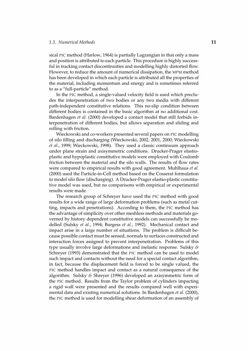
sical PIC method (Harlow, 1964) is partially Lagrangian in that only a massand position is attributed to each particle. This procedure is highly success-ful in tracking contact discontinuities and modelling highly distorted flow.However, to reduce the amount of numerical dissipation, the MPM methodhas been developed in which each particle is attributed all the properties ofthe material, including momentum and energy and is sometimes referredto as a “full-particle” method.
In the PIC method, a single-valued velocity field is used which preclu-des the interpenetration of two bodies or any two media with differentpath-independent constitutive relations. This no-slip condition betweendifferent bodies is contained in the basic algorithm at no additional cost.Bardenhagen et al. (2000) developed a contact model that still forbids in-terpenetration of different bodies, but allows separation and sliding androlling with friction.
Wieckowski and co-workers presented several papers on PIC modellingof silo filling and discharging (Wieckowski, 2002, 2001, 2000; Wieckowskiet al., 1999; Wieckowski, 1998). They used a classic continuum approachunder plane strain and axisymmetric conditions. Drucker-Prager elastio-plastic and hypoplastic constitutive models were employed with Coulombfriction between the material and the silo walls. The results of flow rateswere compared to empirical results with good agreement. Muhlhaus et al.(2000) used the Particle-in-Cell method based on the Cosserat formulationto model silo flow (discharging). A Drucker-Prager elastio-plastic constitu-tive model was used, but no comparisons with empirical or experimentalresults were made.
The research group of Schreyer have used the PIC method with goodresults for a wide range of large deformation problems (such as metal cut-ting, impacts and penetrations). According to them, the PIC method hasthe advantage of simplicity over other meshless methods and materials go-verned by history dependent constitutive models can successfully be mo-delled (Sulsky et al., 1994; Burgess et al., 1992). Mechanical contact andimpact arise in a large number of situations. The problem is difficult be-cause possible contact must be sensed, normals to surfaces constructed andinteraction forces assigned to prevent interpenetration. Problems of thistype usually involve large deformations and inelastic response. Sulsky &Schreyer (1993) demonstrated that the PIC method can be used to modelsuch impact and contacts without the need for a special contact algorithm,in fact, because the displacement field is forced to be single valued, thePIC method handles impact and contact as a natural consequence of thealgorithm. Sulsky & Shreyer (1996) developed an axisymmetric form ofthe PIC method. Results from the Taylor problem of cylinders impactinga rigid wall were presented and the results compared well with experi-mental data and existing numerical solutions. In Bardenhagen et al. (2000),the PIC method is used for modelling shear deformation of an assembly of

1.4. Thesis Goals and Outline 12
granules. A special contact algorithm is used to model the Coulomb fric-tion between the individual granules. In Sulsky et al. (1995) and Sulsky &Schreyer (1993), they have modelled the impact of an elastic steel disk onan elastic-perfectly plastic (von Mises) aluminium target at high velocity.Both plane strain and axisymmetric approaches were used and the resultswere in good agreement with experimental measurements. Schreyer et al.(2002) modelled delamination, a type of failure that can occur in layeredcomposites. The PIC method was used to avoid remeshing and remappingof history variables. The solutions showed no sensitivity of delaminationpropagation with mesh orientation. Shen et al. (2000) studied the deforma-tion characteristics of ductile polycrystalline materials at elevated tempe-ratures by considering a square segment of material subjected to differentstress modes. The PIC method was used to model the polycrystalline mi-crostructure numerically.
A common feature of meshless methods such as the element-free Galer-kin method, is their computational cost and routine use for a wide range ofapplications appears not to be feasible (Schreyer et al., 2002). SPH is muchless complex, but unfortunately this method is subject to instabilities undertensile states of stress and must be applied carefully (Swegle et al., 1995;Schreyer et al., 2002). In comparison with these meshless methods, PIC ap-pears to be considerably less complex. With the use of an explicit timeintegration scheme, the computational cost increase of PIC is about 20%over that associated with the use of low-order finite elements, comparedto current forms of the explicit element-free Galerkin approach where thecost exceeds that of low-order elements by a factor of 4-10 (Schreyer et al.,2002). The PIC method is based on standard FEM, which is used to solvethe equations of motion, conservation of mass and temperature evolution.Advantages include the whole body of theory from FEM, the fact that mostof the code can be standard, and the robustness of the method.
1.4 Thesis Goals and Outline
1.4.1 Goals
Earthmoving equipment is not only used for mining, it also plays an im-portant role in the agricultural and earthmoving industries. The equip-ment is highly diverse in shape and function, but most of the soil cuttingmachines can be categorised into one of three principal classes: blades, rip-pers and buckets or shovels. Tools that resemble blades include bulldozerfront blades, road graders, hauling scrapers, snowplows and other straight-edged blades. These instruments cut and push soil or other granular ma-terial at a depth that is generally less than their width. Ripper type toolsare narrower compared to their working depth and are often attached tobulldozers and graders when it is necessary to cut and loosen hard soil.

1.4. Thesis Goals and Outline 13
Figure 1.1: A typical walking dragline
Buckets are blades equipped with sides that form a space in which soil orother materials can be cut and lifted up. The basic shape of earthmovingtools has not changed a great deal since antiquity, although most are ope-rated today by mechanical power sources and their construction benefitsfrom modern metallurgical engineering.
Draglines are used to remove blasted overburden from open cast mi-nes. Its removal exposes the coal deposits beneath for mining. A dragline,as depicted in figure 1.1, is a crane-like structure with a huge bucket of upto 100 m3 in volume. Draglines are an expensive and essential part of mineoperations and play an important role in the competitiveness of South Af-rican mines. In the coal mining industry it is generally accepted that a 1%improvement in the efficiency of a dragline will result in an R 1 millionincrease in annual production per dragline (Esterhuyse, 1997).
The main goal of this dissertation is to model the flow of loose (cohe-sionless) granular material in front of flat bulldozer blades and into drag-line type buckets using a continuum method. During these processes, thematerial experiences large deformations, free surface flow and the forma-tion of shear bands. All of these must be accurately modelled so that pre-dictions of soil flow patterns and resultant forces and moments on the bladeand bucket are possible.
To reach this goal, a PIC code was developed to model these proces-ses under plane strain conditions. The code called PICCUS (Particle-in-CellCode University of Stellenbosch) is based on both the Cosserat and classiccontinuum formulations. Published numerical and experimental resultswere used to validate the code. Blade and bucket results were compared toexperimental measurements and observations as well as DEM simulations

1.4. Thesis Goals and Outline 14
(Coetzee, 2000).
1.4.2 Novelty
The only known researchers who used the PIC method based on the Cosse-rat continuum are Muhlhaus et al. (2000). They modelled silo and trapdoorflow , i.e. natural gravitational flow. Bohatier & Nouguier (1999) investiga-ted forced flow (blade cutting) but based on the classic continuum formu-lation for history independent material and FEM with remeshing and in theabsence of gravity.
The application of the Particle-in-Cell method based on the Cosseratcontinuum formulation with history-dependent constitutive equations onforced granular flow is unique. Neither Muhlhaus et al. (2000) nor Boha-tier & Nouguier (1999) compared their results with experiments. Tejchman(1996) performed numerical simulations of silo filling with a hypoplasticCosserat continuum and compared his results to that of an experiment. Thesilo was, however, filled layer-by-layer and standard FEM could be usedunder the assumed quasi-static conditions.
The numerical simulation of bucket filling has only been performed byCleary (1998b) and Coetzee (2000). Both authors used discrete element me-thods. The modelling of bucket filling with a continuum method has notyet been done.
1.4.3 Outline
Chapter 2 gives a brief overlook of the Particle-in-Cell method based on theclassic nonpolar continuum formulation. Chapter 3 gives an overview ofthe different boundary conditions and initial conditions that were used.
In Chapter 4, analytical and published numerical data are used to eva-luate and validate the code. Particle-in-Cell simulations performed by otherauthors are repeated to validate the correct implementation of the code.This includes the impact of an elastic steel disk on a perfectly plastic alu-minium target and the discharge of a silo. The analytical solution of a rigiddisk on an inclined plane is used to validate the contact model. Differentvalues of friction coefficient and angles of inclination are used to modeleither a stick-rolling contact or a slip-rolling contact. The impact of twoelastic bodies is modelled to demonstrate the conservation of momentumand energy. The analytical solution of a simple oedometer test is used tovalidate the implementation of a Mohr-Coulomb constitutive model. In anoedometer experiment, two of the principle stress components are equal,and during plastic flow, the stress point evolves along a shear-shear edgeof the Mohr-Coulomb criterion representation in the principal stress space.
The method of characteristics is used to determine the forces acting on aflat blade and the shape of the material shear band. The results for different

1.4. Thesis Goals and Outline 15
blade depths and mesh sizes are compared. The analysis of a strip loadingon an elastic mass is compared to an analytical model. The distribution ofthe major and minor principal stresses below the footing is compared to theanalytical solution.
In Chapter 5 published experimental results are used to evaluate andvalidate the code. Not all of the problems being analysed involve largedisplacements. The simulation of slope stability and anchor pull-out testsfor instance, can be performed with standard FEM codes. It does, however,indicate that these types of applications, typical to civil and geotechnicalengineering, can be modelled using PIC. It also shows that using PIC, nospecial contact elements are needed, between the anchor and the soil forinstance, which is the case when FEM is used.
The polar continuum method is only used in blade, bucket and silo mo-delling. In Chapter 6 the flow of loose granular material in front of a flatbulldozer blade, into an excavator type bucket and the discharge of a silo ismodelled. Blade and bucket results are compared to published experimen-tal data and published DEM results. Silo experiments and DEM simulationswere performed as part of this dissertation and the results compared topolar and nonpolar continuum results.
Chapter 7 concludes with some recommendations and possible furtherwork. Appendix A describes the notations used: index notation and Has-senpflug notation. Appendix B gives an overview of classic continuummechanics and Appendix C describes the Cosserat continuum theory. Ap-pendix D describes rigid body kinematics used in the Cosserat continuumtheory. Appendix E gives the essential finite element theory on which PIC
is based. Only four noded isoparametric elements are treated. In AppendixF, a detailed description of the Particle-in-Cell method based on the Cosse-rat continuum is given. Appendix G describes the PIC contact model. Thismodel is based on Coulomb friction theory. Appendix H and Appendix Idescribe the nonpolar and polar constitutive models respectively. The con-stitutive models and their implementation are described.

Chapter 2
Governing Equations
2.1 Introduction
In this chapter, a brief description of the Particle-in-cell (PIC) method ba-sed on the classic continuum formulation is given. In the first part of thischapter, index notation is used to denote vectors and matrices. In the latterpart, Hassenpflug notation is used (Hassenpflug, 1993) to avoid confusionbetween node numbers and indices. Numerical subscripts indicate nodenumbers and x, y and z indicate coordinate directions. A description of thenotations is given in Appendix A. Plane strain conditions are assumed.A more complete description based on the Cosserat continuum is given inAppendix F.
2.2 Space Discretisation
First, the initial configuration of the body is divided into a number of sub-regions. This is done as depicted in figure 2.1. In the centre of each subre-gion a material point or particle is placed. This material point representsthe subspace, and is given a mass mp. The mass is calculated by assumingthat the whole mass of the subregion is concentrated at the material point.The mass of a material point is constant and does not change with time orposition. The density ρ (xi) represented by this collection of discrete masspoints is approximated using the Dirac delta function,
ρ (xi) =Np
∑p=1
mpδ(xi − xp
i
)(2.2.1)
where xi is an arbitrary position vector, xpi is the position vector at mate-
rial point p, Np is the total number of material points and the Dirac deltafunction is defined as follows:
δ (x− a) =
0 x 6= a∞ x = a
and∫ +∞
−∞δ (x− a) dx = 1 (2.2.2)
For clarity, the equations of motion are derived for a single element only.The whole system would be analysed by assembling the matrices and vec-tors as in standard FEM routines. The mass of each material point is fi-xed which ensures mass conservation. The well known linear momentum
16

2.2. Space Discretisation 17
x1
x2
Element mesh
Subdomain
Material point
Figure 2.1: The element mesh and material points within the subdomains
equation of a continuum is given by (Appendix B),
ρdvi
dt= ρ fi + σij,j (2.2.3)
with vi the velocity vector, fi a vector containing the body forces and σij isthe Cauchy stress tensor. As in FEM, the equation of virtual work is used asthe starting point. The equation of virtual work is obtained by multiplyingequation 2.2.3 by a test (weighted) function wi followed by integration overthe space V which satisfies the boundary conditions:∫
Vρ
dvi
dtwi dV =
∫V
ρ fiwi dV +∫
Vσij,jwi dV (2.2.4)
The specific stress is defined as the stress tensor divided by the materialdensity:
σsij =
σij
ρ→ σij = ρσs
ij (2.2.5)
Substituting this definition of the specific stress into equation 2.2.4, andapplying integration by parts, give
∫V
ρdvi
dtwi dV =
∫V
ρ fiwi dV −∫
Vρσs
ijwi,j dV +∫
Sτiwi dS (2.2.6)
where τi is the surface traction acting on surface S with a unit normal vectornj. Substitution of the discrete density representation, equation 2.2.1, intoequation 2.2.6 and making use of the definition of the Dirac delta function
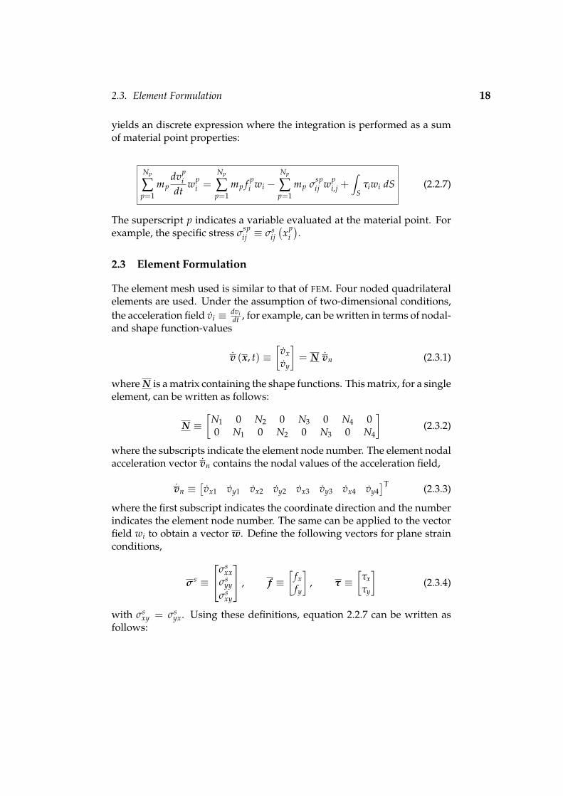
2.3. Element Formulation 18
yields an discrete expression where the integration is performed as a sumof material point properties:
Np
∑p=1
mpdvp
idt
wpi =
Np
∑p=1
mp f pi wi −
Np
∑p=1
mp σspij wp
i,j +∫
Sτiwi dS (2.2.7)
The superscript p indicates a variable evaluated at the material point. Forexample, the specific stress σ
spij ≡ σs
ij(xp
i
).
2.3 Element Formulation
The element mesh used is similar to that of FEM. Four noded quadrilateralelements are used. Under the assumption of two-dimensional conditions,the acceleration field vi ≡ dvi
dt , for example, can be written in terms of nodal-and shape function-values
v (x, t) ≡[
vxvy
]= N vn (2.3.1)
where N is a matrix containing the shape functions. This matrix, for a singleelement, can be written as follows:
N ≡[
N1 0 N2 0 N3 0 N4 00 N1 0 N2 0 N3 0 N4
](2.3.2)
where the subscripts indicate the element node number. The element nodalacceleration vector vn contains the nodal values of the acceleration field,
vn ≡[vx1 vy1 vx2 vy2 vx3 vy3 vx4 vy4
]T (2.3.3)
where the first subscript indicates the coordinate direction and the numberindicates the element node number. The same can be applied to the vectorfield wi to obtain a vector w. Define the following vectors for plane strainconditions,
σ s ≡
σsxx
σsyy
σsxy
, f ≡[
fxfy
], τ ≡
[τxτy
](2.3.4)
with σsxy = σs
yx. Using these definitions, equation 2.2.7 can be written asfollows:

2.3. Element Formulation 19
wTNp
∑p=1
mp
(N p)T
N p vn =
wTNp
∑p=1
mp
(N p)T
fp −wT
Np
∑p=1
mp
(Bp)T
σ sp + wT∫
S
(N p)T
τ dS (2.3.5)
where the superscript p indicates values evaluated at the material points,e.g., N p ≡ N (xp). The arbitrary test vector w appears in all the aboveterms and can thus be dropped. The final discretised system of equationsfollows as
M vn = F int + F ext (2.3.6)
where the mass matrix M is given by
Mij ≡ M =Np
∑p=1
mp
(N p)T
N p (2.3.7)
the internal force vector is given by
F inti ≡ F int = −
Np
∑p=1
mp
(Bp)T
σ sp (2.3.8)
and the external force vector is given by
F exti ≡ F ext =
Np
∑p=1
mp
(N p)T
fp+∫
S
(N p)T
τ dS (2.3.9)
The matrix Bp contains shape function gradients, and for a single elementit can be written as
Bp =
N1,x 0 N2,x 0 N3,x 0 N4,x 00 N1,y 0 N2,y 0 N3,y 0 N4,y
N1,y N1,x N2,y N2,x N3,y N3,x N4,y N4,x
p
(2.3.10)
where the subscripts (, i) are interpreted as the derivatives with respect tothe i global coordinate direction, e.g., N1,x = ∂N1
∂x . In practice, to simplifycomputations, a lumped mass matrix is used instead of the consistent massmatrix given by equation 2.3.7. The lumped mass matrix is a diagonal ma-trix with each entry being the corresponding row sum of the consistentmass matrix. Matrix inversions become trivial if a lumped matrix is used,at the cost of introducing a small amount of numerical dissipation (Burgess

2.4. Time Integration 20
et al., 1992; Brackbill et al., 1988). The consistent mass matrix can also be sin-gular for certain arrangements of the particles. There appears to be only afew arrangements of particles that yield a singular consistent mass matrix,but nearby arrangements might result in an ill-conditioned matrix. On theother hand, the lumped matrix is diagonal and well conditioned.
2.4 Time Integration
Let the time step size be ∆t. The solution to the system of equations 2.3.6is found at discrete instants in time t, t + 1, . . . , t + n. The calculation du-ring each time increment consists of three phases: an initialisation phase, aLangrangian phase and a convective phase.
2.4.1 Initialisation phase
Assume that the position and velocity vector, stress tensor, strain tensorand history dependent variables of each material point are known at timet. With the position of each particle known, its shape function values can becomputed and hence the mass matrix, M t, given by equation 2.3.7. Map-ping of the particle velocities to the nodes is required for the initial data forthe solution to equation 2.3.6. The following equation is solved to obtainthe nodal velocity tvn at time t:
M t tvn =Np
∑p=1
mp
(N p,t
)T[
vp,tx
vp,ty
](2.4.1)
where [vp,t1 vp,t
2 ]T is the material point velocity vector at time t, containingthe velocity components in the x- and y-directions respectively. This equa-tion expresses equivalence of momentum calculated for the material pointsand for the nodes (Wieckowski et al., 1999).
2.4.2 Lagrangian phase
With the shape functions and stresses of each particle known, the internal-and external-force vectors can be calculated using equations 2.3.8 and 2.3.9respectively. With these two vectors and the mass matrix known, equati-ons 2.3.6 is solved for the nodal acceleration at time t:
˙ tvn =(
M t)−1 (
F int,t + F ext,t)
(2.4.2)
The "new" nodal velocity, vnt+1, at time t + 1 is obtained by using an explicit
time integrator:
vnt+1 = tvn + ∆t ˙ tvn (2.4.3)

2.4. Time Integration 21
Using the new nodal velocity, the increment in strains can be calculated atthe particles. Define the vector of strain increment as follows:
∆εp ≡
εpxx
εpyy
εpxy
(2.4.4)
This vector can be calculated using matrix Bp,t,
∆εp,t+1 = ∆t Bp,tvnt+1 (2.4.5)
During the Lagrangian phase the shape function values at the particle po-sitions do not change. Thus, the shape functions and the matrix Bp can beevaluated at time t. With the increment in strain known, the stress state ateach particle can be calculated based on the chosen constitutive model:
∆εp,t+1 constitutive model−−−−−−−−−→ σ p,t+1 (2.4.6)
History dependent variables, such as strain-hardening parameters, mayalso be updated at this stage. During the Lagrangian phase the nodes areassumed to move at the computed nodal velocity vn
t+1. Thus, points in theinterior of the element move in proportion to the motion of the nodes, asgiven by the representation using the nodal shape functions. Since shapefunctions are used to map the nodal velocity continuously to the interiorof the element, the positions of the material points are updated by movingthem in a single-valued, continuous velocity field. Similarly, the velocity ofa material point is updated by mapping the nodal accelerations to the ma-terial point position. The updated material point position vector followsas
xp,t+1 = xp,t + ∆t N p,t vnt+1 (2.4.7)
Similarly, the updated velocity vector is given by
vp,t+1 = vp,t + ∆t N p,t ˙ tvn (2.4.8)
Because the velocity field is single-valued, interpenetration of material isprecluded. This feature of the algorithm allows simulations of impact andpenetration without the need for a special contact algorithm.
2.4.3 Convective phase
At this point in the computational cycle, the material points are completelyupdated and carry the complete solution, i.e., all the state variables neededto start a new calculation step are carried by the material points. Duringthe convective phase, the material points are held fixed and the element

2.5. Stability 22
mesh can be redefined. The mesh can be chosen in any convenient man-ner, for example adaptive meshes can be used to resolve sharp gradientsand interfaces. The simplest and most convenient choice is, however, tokeep the existing mesh. Since the material points do not move during theconvective phase, material point properties have the same value at the endof the convective phase as they had at the end of the Lagrangian phase.This completes the computational cycle. A new cycle is begun using theinformation carried by the material points to initialise nodal values on theelement mesh.
2.5 Stability
In the previous sections, a simple explicit time integrator is used of whichthe time step should satisfy the stability condition, i.e., the critical time stepshould be the smallest ratio of the element size to the wave speed throughthe material. For small displacements, the spatial discretisation in PIC isequivalent to that of FEM using Gauss points at the same locations as thoseof the material points in each element. Therefore, the convergence beha-viour of the integrator used is similar to that employed to integrate the cor-responding equations in FEM. However, according to Chen et al. (2002), noconsistent theoretical results have been obtained for the convergence beha-viour of time integrators when larger deformations occur and a reasonabletime step is usually found through numerical experiments.
2.6 The Polar Continuum
In the previous sections a description of the PIC method was given basedon the classic continuum. In Appendix F, a more detailed description isgiven of PIC, based on the Cosserat continuum. In this section the Cosse-rat continuum is briefly discussed. A detailed description of the Cosseratcontinuum theory is given in Appendix C.
The kinematics of Cosserat continua are characterised by rotational de-grees of freedom wc
i , which are independent of the translation describedby the displacement field ui. Thus, the field of continuum macro-rotationsno longer coincides with that of micro-rotations at each material point. Themicro-rotation wc
i differs from the classical macro-rotation wi since three ro-tational degrees-of-freedom are introduced in addition to the conventionalthree translational degrees-of-freedom. Under two-dimensional conditionseach material point has two translational degrees-of-freedom and one rota-tional degree-of-freedom wc
3.For the formulation of constitutive relationships, deformation measures
which are invariant with respect to rigid body motions are needed. In the
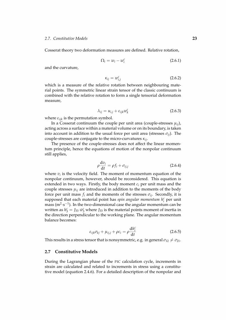
2.7. Constitutive Models 23
Cosserat theory two deformation measures are defined. Relative rotation,
Ωi = wi − wci (2.6.1)
and the curvature,
κij = wci,j (2.6.2)
which is a measure of the relative rotation between neighbouring mate-rial points. The symmetric linear strain tensor of the classic continuum iscombined with the relative rotation to form a single tensorial deformationmeasure,
λij = ui,j + ε ijkwck (2.6.3)
where ε ijk is the permutation symbol.In a Cosserat continuum the couple per unit area (couple-stresses µij),
acting across a surface within a material volume or on its boundary, is takeninto account in addition to the usual force per unit area (stresses σij). Thecouple-stresses are conjugate to the micro-curvatures κij.
The presence of the couple-stresses does not affect the linear momen-tum principle, hence the equations of motion of the nonpolar continuumstill applies,
ρdvi
dt= ρ fi + σij,j (2.6.4)
where vi is the velocity field. The moment of momentum equation of thenonpolar continuum, however, should be reconsidered. This equation isextended in two ways. Firstly, the body moment ci per unit mass and thecouple stresses µij are introduced in addition to the moments of the bodyforce per unit mass fi and the moments of the stresses σij. Secondly, it issupposed that each material point has spin angular momentum hc
i per unitmass (m2·s−1). In the two-dimensional case the angular momentum can bewritten as hc
3 = J33 wc3 where J33 is the material points moment of inertia in
the direction perpendicular to the working plane. The angular momentumbalance becomes:
ε ijkσkj + µij,j + ρci = ρdhc
idt
(2.6.5)
This results in a stress tensor that is nonsymmetric, e.g. in general σ12 6= σ21.
2.7 Constitutive Models
During the Lagrangian phase of the PIC calculation cycle, increments instrain are calculated and related to increments in stress using a constitu-tive model (equation 2.4.6). For a detailed description of the nonpolar and

2.7. Constitutive Models 24
polar constitutive models and their implementation, see Appendix H andAppendix I respectively.
Nonpolar elastic, Drucker-Prager and Mohr-Coulomb models were used.The Drucker-Prager (FLAC, 1998) model is expressed in terms of two gene-ralised stress components: the tangential stress q and mean normal stress pdefined as
q =√
J2
p = 13 (σ11 + σ22 + σ33)
(2.7.1)
where J2 is the second invariant of the stress deviator tensor. The failurecriteria is described in the pq-plane, with the shear yield function given by
f s = q + qφ p− kφ (2.7.2)
and the tension yield function (tension cutoff) by
f t = p− σt (2.7.3)
where qφ and kφ are constant material properties and σt is the material ten-sile strength. The constant qφ is related to the material friction angle. Theshear potential function gs corresponds in general to a non-associated flowrule and has the form
gs = q + qψ p (2.7.4)
where qψ is a material constant related to the material dilatancy angle. Withqψ equal to qφ, the flow rule is termed associated, otherwise it is called non-associated. The flow rule for tensile failure is associated and given by
gt = p (2.7.5)
With the current stress state known, the new stress state is calculatedusing a single-step return algorithm. The algorithm assumes that the totalstrain increment is elastic which is then used to calculate an increment instress. This stress increment is then added to the current stress state toobtain the trial stress state. The trial stress state is then checked against thefailure criteria (shear and tension). If either of the failure criteria is violated,a one step return algorithm is used to bring the trial stress state back to theyield surface using the two potential functions respectively.
The Mohr-Coulomb model (FLAC, 1998) with tension cutoff has a non-associated shear flow rule and an associated tensile flow rule. The shearand tension yield functions are given by
f s = σ1 − σ3Nφ + 2c√
Nφ
f t = σt − σ3
(2.7.6)

2.7. Constitutive Models 25
where σ1 and σ3 are principal stresses with σ1 ≤ σ3, σt is the material tensilestrength, c the cohesion and
Nφ =1 + sinφ
1− sinφ(2.7.7)
with φ the material friction angle. The shear and tension potential functionsare given by
gs = σ1 − σ3Nψ
gt = −σ3(2.7.8)
where
Nψ =1 + sinψ
1− sinψ(2.7.9)
and ψ is the material dilatancy angle. The same single-step return algo-rithm used in the Drucker-Prager model, is used in the Mohr-Coulombmodel.
In the principal stress space, the Drucker-Prager shear criterion is re-presented by a cone with its axis along the line σ1 = σ2 = σ3. The Mohr-Coulomb shear criterion is represented by an irregular hexagonal pyramid.The parameters qφ and kφ can be adjusted so that the Drucker- Prager conewill either pass through the outer or the inner edges of the Mohr-Coulombpyramid (FLAC, 1998). For outer adjustment,
qφ =6√
3 (3− sinφ)sinφ
kφ =6√
3 (3− sinφ)c cosφ
(2.7.10)
and for inner adjustment,
qφ =6√
3 (3 + sinφ)sinφ
kφ =6√
3 (3 + sinφ)c cosφ
(2.7.11)
A polar elastic and Drucker-Prager model were used. In formulatingCosserat elasticity and elasto-plasticity, it is useful to make use of gene-ralised curvatures, e.g. κ31l, where l is a material parameter with the di-mension of length. It is this parameter which effectively sets the internallength scale in the continuum, and therefore has the role of a “charac-teristic length”. Assuming plane strain conditions, the strain and stress

2.7. Constitutive Models 26
components can be assembled in two vectors, de Borst (1991) and de Borst(1993):
εc = [λ11 λ22 λ33 λ12 λ21 κ31l κ32l]T (2.7.12)
σ c =[σ11 σ22 σ33 σ12 σ21
µ31
lµ32
l
]T(2.7.13)
Note that by multiplying the curvatures by the length parameter l, all com-ponents of the strain vector have the same dimension. The couple-stressesare divided by the characteristic length to obtain a stress vector in whichall the entries have the same dimension.
Assuming that the elastic strain vector is linearly related to the stressvector, the following equation can be written
σ c = Deεce (2.7.14)
where De is the stiffness matrix containing the elastic moduli:
De =
2Gc1 2Gc2 2Gc2 0 0 0 02Gc2 2Gc1 2Gc2 0 0 0 02Gc2 2Gc2 2Gc1 0 0 0 0
0 0 0 (G + Gc) (G− Gc) 0 00 0 0 (G− Gc) (G + Gc) 0 00 0 0 0 0 2G 00 0 0 0 0 0 2G
(2.7.15)
with c1 = 1−ν1−2ν and c2 = ν
1−2ν , G is the shear modulus and v Poisson’sratio. Gc is an additional material constant, completing the four materialconstants that are needed to describe the elastic behaviour of an isotropicCosserat continuum under planar deformations. The coefficient 2 has beenintroduced in terms De
66 and De77 in order to arrive at a convenient form of
the elasto-plastic constitutive equations. The total (bending) stiffness thatsets the relation between the micro-curvatures and the couple stresses isbasically determined by the value of the internal length scale l.
The Cosserat Drucker-Prager model used was proposed by Muhlhaus(1987). The yield function f is given by
f = q + α(γ)p− c (2.7.16)
and the potential function g by
g = q + β(γ)p (2.7.17)

2.7. Constitutive Models 27
where
q =√
J2 (2.7.18)
and
p =12
(σ11 + σ22 + σ33) (2.7.19)
The second invariant of the deviatoric stress tensor J2 is given by:
J2 = a1sijsij + a2sijsji +a3µijµij
l2 (2.7.20)
where sij is the deviatoric stress tensor, α is a friction factor, β a dilatancyfactor, c is cohesion, γ the hardening parameter and a1, a2 and a3 are mate-rial parameters. Muhlhaus (1987) derived, on a macroscopic level and bytaking into account slip and rotation in a random assembly of circular rodswith a fixed diameter, the following set of parameters: a1 = 3
8 , a2 = 18 and
a3 = 1. This set is referred to as the standard set. From micromechanicalconsiderations it was also shown by Muhlhaus & Vardoulakis (1987) that:
Gc =G
2 (a1 − a2)(2.7.21)
The new stress state is calculated using an iterative trial stress method.An elastic predictor and a plastic corrector with radial return mapping isused and convergence is achieved within two to three iterations (Tejchman,1997).
A rigid body model was also implemented and used for the modellingof strip footings, anchors, blades and buckets.

Chapter 3
Boundary and Initial Conditions
3.1 Introduction
Correctly specified boundary and initial conditions are needed to obtainspecific solutions of the partial differential equations that describe the me-chanics of granular flow. This chapter gives an overview of the differentboundary and initial conditions used.
3.2 Boundary Conditions
In general, boundary conditions can be either fixed boundaries, appliedtraction or absorbing boundaries. In fixed boundaries, displacement androtation can be fixed in one or more of the coordinate directions.
Modelling sometimes involves media which, at the scale of the analysis,are better represented as unbounded. An unbounded medium can be mo-delled as a bounded medium if the correct artificial numerical boundariesare enforced. In static analyses, fixed boundary conditions can be placed atsome distance from the region of interest. In dynamic simulations, howe-ver, such boundaries lead to the reflection of outward propagating wavesback into the model. The use of a large enough model would minimisethe problem, since material damping will absorb most of the energy in thewaves reflected from the boundaries. The alternative is to use absorbingboundaries of which the viscous boundary developed by Lysmer & Kuhle-meyer (1969) and Kunar et al. (1977) is an example.
In PICCUS nodes can be fixed in one or more of the coordinate directionsor a constant traction (pressure) can be applied. In all the models wherethe reflection of waves from the boundaries could have an influence onthe results, the models were made large enough for the reflecting waves tohave no significant effect. No absorbing boundaries were used.
In the basic PIC algorithm no slip contact between different bodies isachieved without additional cost. This is the result of the bodies moving ina single-valued velocity field. A contact model developed by Bardenhagenet al. (2000) was used to apply Coulomb friction at the boundary nodes ofcontacting entities. This model allows no interpenetration of the entities inthe contact normal direction, but do allow frictional slip in the tangentialdirection. A detailed description of the contact model and its implementa-tion is given in Appendix G.
Strip footings, anchors, blades and buckets were modelled as rigid bo-dies. The contact model was used to model the contact between these rigid
28

3.3. Initial Conditions and Damping 29
bodies and the granular material by specifying the friction coefficient µ.The Cosserat rotation at the contacting interface could either be free or fi-xed (wc
3 = 0).The roughness of a wall can quantitatively be characterised by the ave-
rage distance rw from the peak to the valley of asperities (Tejchman, 1997).It is, however, the ratio between the wall roughness and the mean grain dia-meter, rw
d50, that determines the interface behaviour between the wall and the
grains. According to Tejchman (1997) no rotation should be allowed at re-latively smooth interfaces. Tejchman (1997) reports that shear tests on sandshowed that in the case of rough surfaces, particles experience both slidingand rotation. In the case of smooth surfaces the sand mass simply slidedalong the surface with very little rotation. The rotation along a smooth sur-face was about 200 times smaller than for rough walls. A smooth interfaceis defined when rw
d50< 0.1.
3.3 Initial Conditions and Damping
In many situations the precise initial stress field is not known. In some sim-ple cases it can be calculated analytically, but for most practical problems,this is not possible. It is, however important to specify realistic initial con-ditions, since it can have an influence on the results and the stability of thecomputation.
In PICCUS, the initial velocity and/or stresses at a material point canbe specified. When the initial velocity is specified, only a uniform velocityfield can be used, i.e., the velocity of all material points will be the same.Different methods of specifying the initial stresses are provided in PICCUS.
3.3.1 Uniform Stress Field
Using this method, a uniform stress field is created by specifying the indivi-dual stress components σ11, σ12 = σ21, σ22 and σ33 for a nonpolar continuumand σ11, σ12, σ21, σ22, σ33, µ31 and µ31 for a Cosserat continuum. Care shouldbe taken since the initial conditions may cause the material not to be inequilibrium and it may also violate the yield criterion.
A uniform initial stress field is a realistic approach for deep under-ground excavations. In such a case, the gravitational variation of stressfrom top to bottom of the excavation may be neglected because the va-riation is small in comparison with the magnitude of stress acting on thevolume of material to be modelled.
3.3.2 Stress Field with a Gradient
Near the ground’s surface, the variation in stress with depth cannot beignored. In a uniform layer of soil with a horizontal free surface, the ver-

3.3. Initial Conditions and Damping 30
tical stresses (σ22) are usually equal to −ρgh, where g is the magnitude ofthe gravitational acceleration in the vertical direction (x2) and usually ta-ken as g = 9.81 m·s−2. Note that this results in a negative value in σ22,i.e. a compressive stress. The mass density of the material is denoted by ρand h is the depth below the free surface. However, the horizontal stresses(σ11 and σ33) are more difficult to estimate. It is common to represent theratio of horizontal to vertical effective stress by the "in rest" coefficient, Tinget al. (1994):
Ko =σh
σv⇒ σh = Ko σv (3.3.1)
Under the assumption that gravity is suddenly applied to an elastic massof material, initially stress free, in which lateral movement is prevented, itcan be shown that
Ko =ν
1− ν(3.3.2)
where ν is Poisson’s ratio. For natural soil this condition hardly ever app-lies in practice (FLAC, 1998) due to repeated tectonic movements, materialfailure, overburden removal and locked-in stresses due to faulting and lo-calisation. Of course, if enough knowledge of the history of the particularvolume of material is available, it is possible to simulate the whole processnumerically, to arrive at the initial conditions. This approach is seldomfeasible. Several theoretical and empirical relationships for Ko have beenpostulated for natural soil. Probably the simplest and most widely knownis the approximation to the theoretical formula by Jaky (1944):
Ko = 1− sin(φ) (3.3.3)
where φ is the material friction angle. This method of estimating the initialstresses, of course, is only applicable when the free surface is horizontaland without steps.
3.3.3 Layer-by-Layer Method
Figure 3.1 shows the configuration of a blade or wall typically used to mo-del retaining walls or earthmoving equipment respectively. The bottomand side boundaries can be either fixed in one or more of the coordinate di-rections. A layer-by-layer method is used to generate initial stresses. Onelayer of material is created, starting at the bottom, with initial stresses givenby

3.3. Initial Conditions and Damping 31
10
1
2
3
4
56
78
9
Soil free surface
Wall / Blade
Soil free surface
Bottom boundary
Side
bou
ndar
y
Side
bou
ndar
yx1
x2
Figure 3.1: Layer-by-layer method of generating initial stresses
σ22 = −ρghσ11 = Koσ22
σ33 = Koσ22
σ12 = σ21 = 0µ31 = µ32 = 0 only for Cosserat continuum
(3.3.4)
where Ko = 1 − sin(φ) and h the height measured from the free surfaceof the current layer to the material point. With gravity activated, heavydamping is applied until static equilibrium is reached, equilibrium beingdefined when the maximum value in particle velocity is smaller or equalto 1× 10⁻⁸ m·s−1. After an equilibrium state has been reached, the nextlayer is added. This procedure is followed until the bottom edge of thewall/blade is reached. The wall/blade is then created and material ad-ded to the right of the wall/blade, layer-by-layer. The wall/blade may besmooth or have a specified friction.
In order to obtain the static equilibrium state, the equations of motionmust be damped. The objective is to achieve the steady state in a nume-rically stable way with minimal computational effort. A form of dampingcalled local non-viscous damping was implemented in which the dampingforce on a node is proportional to the magnitude of the unbalanced forceat the node (FLAC, 1998). The direction of the damping force is such thatenergy is always dissipated. The damping force is simply added to theequation of motion, equation 2.3.6, and is given by
Fidamp = −α
∣∣∣Fiint + Fi
ext∣∣∣ sign(vn) (3.3.5)
where vn is the nodal velocity vector and α the damping factor. For a detai-led description of the damping implementation see Appendix G.

Chapter 4
Numerical and Analytical Validation
4.1 Introduction
In order to use PICCUS for practical applications, it should be thoroughlyevaluated and validated. In this chapter, published numerical data as wellas analytical results are used to validate the code. Some of the simulationsare exactly the same as performed by other authors using PIC, thus thoseonly validate the implementation of the code.
4.2 Simulation of a High Velocity Impact
This simulation consists of an AISI 52-100 chromium steel disk impactingan elastic-perfectly plastic target of 6061-T6 aluminium under plane strainconditions. The material properties are summarised in table 4.1. The alu-minium target has dimensions of 60 mm wide and 40 mm high. The steeldisk has a diameter of 9.53 mm and an initial velocity of 1160 m·s−1. Thesteel disk is assumed to be linear elastic and the aluminium target to beelastic-perfect plastic and obeying a von Mises yield criterion. The yieldstress σy is the yield stress for the material in simple tension.
The computational domain is 60× 60 mm in size and consists of 50× 50elements, i.e the size of one element is 1.2× 1.2 mm. There are, initially, 4particles per element. No contact model is used, so the contact interfacebetween the disk and the target is a non-slip contact. All the boundariesare fixed.
Figure 4.1 shows the penetration after 24 µs, computed by Sulsky &Schreyer (1993). Figure 4.2 shows the penetration at the same time, usingPICCUS.There are differences in the position of individual particles, but this mightbe as a result of the original positions of the particles within the elements,
Table 4.1: Material properties used in impact simulation
Description Symbol Steel Aluminium
Young’s modulus E 200 GPa 78.2 GPa
Density ρ 7850 kg·m−3 2700 kg·m−3
Poisson’s ratio ν 0.3 0.3
Yield stress σy - 300 MPa
32

4.2. Simulation of a High Velocity Impact 33
Figure 4.1: Penetrated configuration at t = 24 µs, (Sulsky and Schreyer, 1993)

4.2. Simulation of a High Velocity Impact 34
Figure 4.2: Penetrated configuration at t = 24 µs, (PICCUS)
which were not given by Sulsky & Schreyer (1993). Figure 4.3 shows thepenetration depth as a function of time. Here it can be seen that the pene-tration predicted by PICCUS is in close agreement with the published datafrom Sulsky & Schreyer (1993).
The final depth of penetration is 19 mm. Silling (1992) made use of anEulerian code, CTH, and obtained a final penetration depth of 20 mm. Tru-cano & Grady (1985) performed experiments and measured a final pene-tration depth of 21 mm. Sulsky & Schreyer (1993) showed that the resultsfrom plane strain (19 mm) and plane stress (25 mm) conditions bracket theexperimental result, while Sulsky et al. (1995) made use of two-dimensionalaxisymmetric cylindrical coordinates and obtained a final depth of 18 mm.The experimental data shows that the sphere is more or less undeformedafter penetration (Trucano and Grady, 1985).
Figures 4.4 to 4.10 show the configuration at different times during the
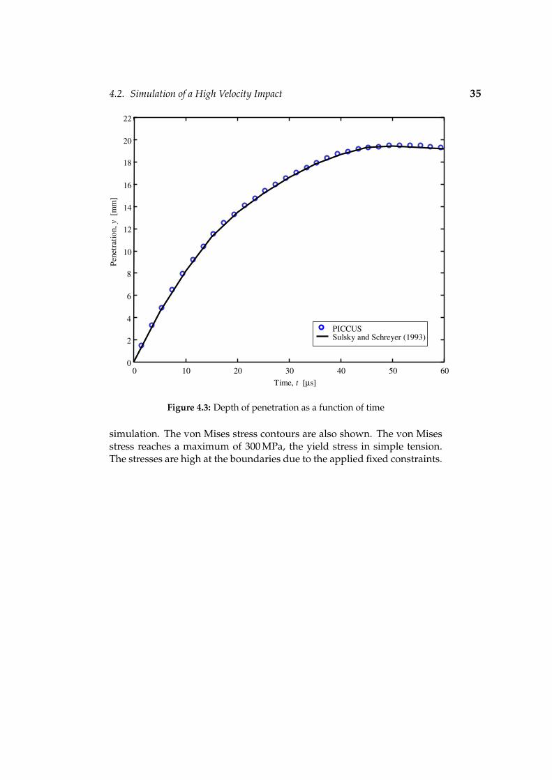
4.2. Simulation of a High Velocity Impact 35
0 10 20 30 40 50 600
2
4
6
8
10
12
14
16
18
20
22
Time, t [µs]
Pene
trat
ion,
y [
mm
]
PICCUS Sulsky and Schreyer (1993)
Figure 4.3: Depth of penetration as a function of time
simulation. The von Mises stress contours are also shown. The von Misesstress reaches a maximum of 300 MPa, the yield stress in simple tension.The stresses are high at the boundaries due to the applied fixed constraints.

4.2. Simulation of a High Velocity Impact 36
Figure 4.4: Penetration at t = 0 µs, particles configuration and von Mises stress
Figure 4.5: Penetration at t = 3.2 µs, particles configuration and von Mises stress

4.2. Simulation of a High Velocity Impact 37
Figure 4.6: Penetration at t = 6.4 µs, particles configuration and von Mises stress
Figure 4.7: Penetration at t = 9.6 µs, particles configuration and von Mises stress
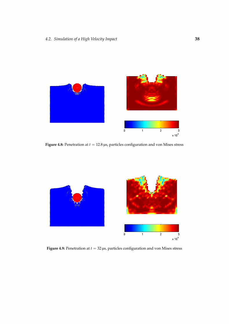
4.2. Simulation of a High Velocity Impact 38
Figure 4.8: Penetration at t = 12.8 µs, particles configuration and von Mises stress
Figure 4.9: Penetration at t = 32 µs, particles configuration and von Mises stress

4.3. Inclined Plane Simulation 39
Figure 4.10: Penetration at t = 80 µs, particles configuration and von Mises stress
4.3 Inclined Plane Simulation
Without the use of a special contact model, all contacts are automaticallyhandled as non-slip contacts in the PIC method. This is a direct result of thesingle-valued velocity field used to update the particle positions. In orderto model slip, a special contact algorithm must be employed. The modelused in PICCUS assumes a Coulomb friction model. This allows frictionalslip in the tangential contact direction and no interpenetration in the con-tact normal direction. This model is described by Bardenhagen et al. (2000)and the PICCUS implementation is given in Appendix G.
The simple case of an cylinder rolling down an inclined plane is usedto demonstrate the ability of PICCUS to model Coulomb frictional contacts,figure 4.11a. The plane is inclined at an angle of θ to the horizontal, whilegravity acts vertically down. Figure 4.11b shows the geometry for the simu-lation where the plane is aligned with the computational boundary, wherefriction is applied, and gravity makes an angle θ to the vertical. If the diskis rigid, its centre-of-mass velocity is tangent to the surface of the inclinedplane, figure 4.11a, and tangent to the horizontal boundary, figure 4.11b.
A rigid disk on an inclined plane will either roll and stick at the contactpoint or roll and slip at the contact point. Whether the disk sticks or slipsdepends on the coefficient of friction and the inclination angle. It can beshown that if tanθ > 3µ the disk will roll and slip (µ is the coefficient offriction), otherwise the disk will roll without slipping. For a rigid disk,starting from rest, the x1-component of the centre position as a function of

4.3. Inclined Plane Simulation 40
v
x1
x2
θg
(a)
x2
x1
v
gθ
(b)
Figure 4.11: (a) Cylinder on an inclined plane, (b) Geometry for simulation ofcylinder on inclined plane
time is given by equation 4.3.1.
x1(t) =
xo + 1
2 |g|t2(sinθ − µcosθ), tanθ > 3µ (slip)xo + 1
3 |g|t2sinθ, tanθ 6 3µ (stick)(4.3.1)
where xo is the initial centre position.Simulations were performed with a linear elastic disk with a radius of
0.5 m and gravitational acceleration of magnitude 9.81 m·s−2. The compu-tational domain had a size of 1.625× 1.250 m with 26× 20 square elements,i.e. 16 elements across the disk diameter. There are initially 4 particlesper element. The disk has a shear modulus G = 2.5 MPa, a bulk modulusK = 10 MPa and a density of ρ = 3000 kg·m−3. The stresses at the particlesare initialised with a value given by the solution to the plane strain staticproblem, σ11 = σ22 = −ρgh, σ33 = ν(σ11 + σ22), where g is the magni-tude of the gravitational acceleration and h is the position of the materialpoint measured from the top free surface of the disk (Timoshenko and Goo-dier, 1970). Figure 4.12 shows the disk after 0.3 seconds with θ = 60 andµ = 0.9, i.e. a roll and stick contact occurs. The velocity vector of eachmaterial point is shown, scaled to one-tenth.
Figure 4.13 shows the centre displacement (x1-component) as a functionof time for θ = 60 and µ = 0.3 (slip), θ = 30 and µ = 0.1 (slip) and θ = 60

4.3. Inclined Plane Simulation 41
0 0.2 0.4 0.6 0.8 1 1.2 1.4 1.60
0.2
0.4
0.6
0.8
1
1.2
Figure 4.12: Disk at time t = 0.3 s, θ = 60, µ = 0.9. Velocity vectors V−→10
Table 4.2: The effect of mesh refinement on inclined plane simulation
Mesh size # Particles Initial DOF Running time Error at t = 0.3 s
26 × 20 812 510 415 s 14.60 %
52 × 40 3228 1788 2128 s 6.40 %
104 × 80 12892 6780 23 400 s 0.56 %
Computing times with dt = 1× 10⁻⁵ s, θ = 60, µ = 0.9
and µ = 0.9 (stick). The errors in centre position calculated at t = 0.3 s are0.05%, 0.50% and 0.56% respectively. Mesh sizes of 26× 20, 52× 40 and104 × 80 were used to investigate mesh dependency. With a finer meshthe results are more accurate, as expected, and it also shows convergence.The number of particles, running times and accuracy are summarised in ta-ble 4.2. The simulations were run on an AMD 1.33GHz with 512 MB RAM.

4.4. Impact of Two Elastic Bodies 42
0 0.05 0.1 0.15 0.2 0.25 0.30
0.05
0.1
0.15
0.2
0.25
0.3
0.35
Time [s]
Cen
tre
disp
lace
men
t [m
]
θ = 60°, µ = 0.3, 26 × 20
θ = 30°, µ = 0.1, 26 × 20
θ = 60°, µ = 0.9, 104 × 80
The solid lines indicate analytical solutions.
Figure 4.13: Inclined plane simulation: Centre position for different incline angles,friction coefficients and mesh sizes
4.4 Impact of Two Elastic Bodies
The simple impact of two elastic disks were analysed to evaluate the con-servation of momentum and energy. Figure 4.14 shows the two disks attime t = 0. The domain size is 1.0× 1.0 m with 25 elements in each direc-tion. With initially 4 particles per element, each disk has 316 particles. Eachdisk has a diameter of 0.4 m. Simulations are performed in the absence ofgravity. The material density is ρ = 1000 kg·m−3, Young’s modulus E =1000 Pa and Poisson’s ratio ν = 0.3. Figure 4.15 to figure 4.17 show thedisks at the point of contact, minimum kinetic energy and the point wherecontact is broken respectively. The contact between two bodies A and B isdefined at the contacting nodes and not the material points and therefore itseems as if there is a gap between the two bodies in contact. Nodal contactoccurs when a node is common to two elements, say 1 and 2, and element 1contains at least one material point belonging to say entity A, and element2 contains at least one material point belonging to entity B.

4.4. Impact of Two Elastic Bodies 43
Figure 4.14: Initial positions of the disks at time t = 0.00 s
Figure 4.15: Positions of the disks at the point of contact, t = 1.30 s

4.4. Impact of Two Elastic Bodies 44
Figure 4.16: Positions of the disks at the point of minimum kinetic energy, t =1.96 s
The disks start in the upper left and lower right hand corners with in-itial velocity components of (0.1,−0.1) and (−0.1, 0.1) m·s−1 respectively.Figure 4.18 shows the x1- and negative x2- components of the momentumfor the disk starting in the upper left hand corner. A time step of ∆t =1× 10⁻⁵ s was used. There is no error in the numerical solution associatedwith a uniform translation of the disk through the grid. This can be seenby the fact that there is no change in momentum over the first 1.30 s, i.e.up to the point of contact. The disks rebound and translate in the oppositedirection after the impact has occurred and the momentum switches sign.The negative of the x2-component of momentum is indistinguishable fromthe x1-component both before and after impact, which is expected as thedisplacement of the disk makes an angle of 45 with respect to the axis.The x1-momentum at time t = 4.00 s is slightly less than at time t = 0.00 s,but with the error being only 0.235% it is acceptable.
Figure 4.19 shows the energy plots. All of the initial energy is kineticenergy. The kinetic energy decreases during impact and is then mostlyrecovered after separation. The strain energy reaches its maximum valueat the point of maximum deformation during impact and then decreases toa value associated with free vibration of the disk. After impact, the strainenergy is small, but not zero. The fact that a zero value is not achieved canbe attributed to the activation of several modes which do not exhibit zerosat the same time (Sulsky et al., 1994).
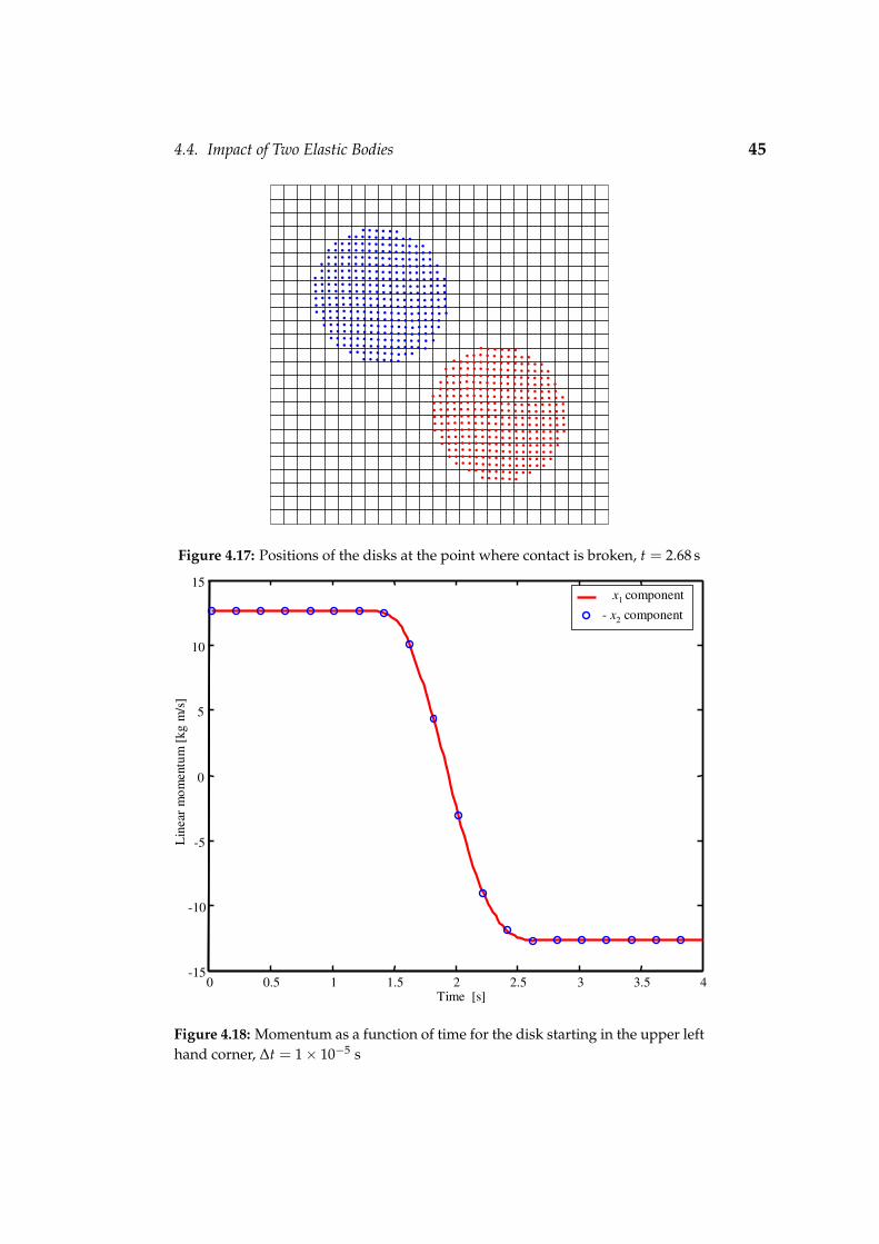
4.4. Impact of Two Elastic Bodies 45
Figure 4.17: Positions of the disks at the point where contact is broken, t = 2.68 s
0 0.5 1 1.5 2 2.5 3 3.5 4-15
-10
-5
0
5
10
15
Time [s]
Lin
ear
mom
entu
m [k
g m
/s]
x1 component - x2 component
Figure 4.18: Momentum as a function of time for the disk starting in the upper lefthand corner, ∆t = 1× 10⁻⁵ s

4.4. Impact of Two Elastic Bodies 46
0 0.5 1 1.5 2 2.5 3 3.5 40
0.5
1
1.5
2
2.5
3
Time [s]
Ene
rgy
[J]
KineticStrain Total
Figure 4.19: Energy as a function of time, ∆t = 1× 10⁻⁵ s. No slip contact

4.4. Impact of Two Elastic Bodies 47
0 0.5 1 1.5 2 2.5 3 3.5 4-0.25
-0.2
-0.15
-0.1
-0.05
0
0.05
0.1
0.15
Time [s]
Ene
rgy
gain
/dis
sipa
tion
[%]
∆t = 1×10⁻³ s∆t = 1×10⁻⁴ s∆t = 1×10⁻⁵ s
Figure 4.20: Gain/Dissipation in total energy as a percentage of the total energy att = 0. Gain being positive and dissipation negative. No slip contact

4.4. Impact of Two Elastic Bodies 48
Table 4.3: Energy gain/dissipation using different time steps
Time step Max gain Max dissipation
1× 10⁻³ s 0.104 % 0.208 %
1× 10⁻⁴ s 0.010 % 0.021 %
1× 10⁻⁵ s 0.001 % 0.002 %
Figure 4.20 shows the dissipation and/or gain in total energy as a per-centage of the energy at time t = 0 for different time steps. For the timeup to contact, there is no dissipation or gain in energy. During and aftercontact, however, there are some dissipation and gain. As expected, with adecrease in the size of the time step, there is a decrease in error. Table 4.3summarises the results.
In the above simulations no contact model was used, i.e. no slip con-ditions were assumed. If the contact model is used, Coulomb friction bet-ween the two disks can be modelled. A friction coefficient of µ = 0.1 wasassumed. It took 36 s to complete a simulation assuming no slip, and app-lying the contact model, the simulation took 42 s. When the contact modelis used, boundary nodes must be found each time step and the unit nor-mal vector calculated at contacting nodes before a contact correction can beapplied. Thus the 16.7% increase in computation time.

4.4. Impact of Two Elastic Bodies 49
0 0.5 1 1.5 2 2.5 3 3.5 40
0.5
1
1.5
2
2.5
3
Time [s]
Ene
rgy
[J]
KineticStrain Total
Figure 4.21: Energy as a function of time, ∆t = 1× 10⁻⁵ s, µ = 0.1

4.5. Oedometer Test 50
0 0.5 1 1.5 2 2.5 3 3.5 4-6
-5
-4
-3
-2
-1
0
1
Time [s]
Ene
rgy
diss
ipat
ion
[%]
No slip
µ = 0.1
Figure 4.22: Gain/Dissipation in total energy as a percentage of the total energy att = 0. Gain being positive and dissipation negative, ∆t = 1× 10⁻⁵ s
Figure 4.21 shows the total energy as a function of time when the Coulombfriction model is used. It can be seen that during impact there is a loss intotal energy, but after impact, there is no additional dissipation. Figure 4.22shows the dissipation as a percentage of the total energy at t = 0. On thescale used in this figure, there is no discernable dissipation when a no slipcontact is assumed.
4.5 Oedometer Test
This example (FLAC, 1998) is used to evaluate the ability of the code todetermine stresses in a Mohr-Coulomb material subjected to an oedome-ter test. In the principal stress space the Mohr-Coulomb shear criterion isrepresented by an irregular hexagonal pyramid (Appendix H). In an oe-dometer experiment, two of the principal stress components are equal, andduring plastic flow, the stress point evolves along an edge of the pyramid.The purpose of this simulation is to indicate that the Mohr-Coulomb mo-del as implemented in PICCUS, can handle such a situation. Results arecompared to analytical solutions.

4.5. Oedometer Test 51
x1
x2
V V
Figure 4.23: Boundary conditions for oedometer test (FLAC, 1998)
Table 4.4: Material properties used in oedometer test
Description Symbol ValueBulk modulus K 200 MPaShear modulus G 200 MPaCohesion c 1 MPaFriction angle φ 10
Dilatancy angle ψ 10 and 0
Tensile limit σt 5.67 MPa
The boundary conditions for the plane strain oedometer test are shown infigure 4.23. This corresponds to the uniform strain rates
∆ε11 = 0
∆ε22 =V∆t
L∆ε33 = 0∆ε12 = ∆ε21 = 0
(4.5.1)
Since the shear stresses are all zero, the normal stresses are principal stres-ses. A constant velocity V is applied to the sample (V < 0) with a heightL.
The application of Hook’s law and the Mohr-Coulomb yield criterionleads to a closed-form solution to this problem (Appendix H). This analy-tical solution is compared to a numeric experiment using one element with9 particles (3x3), figure 4.24. A rigid body plunger is used to induce theconstant velocity at the upper boundary. The plunger also has 9 particlesin a single element and the contact between the plunger and the Mohr-

4.5. Oedometer Test 52
Figure 4.24: Oedometer test: Simulation setup with 9 particles per element. Plun-ger material point velocity vectors v−→
100
Coulomb material is frictionless, i.e. perfectly smooth. The other boundaryconditions are the same as in figure 4.23. The material properties used areshown in table 4.4.
A time step of 1× 10⁻⁶ s, and a velocity of 10 m·s−1 were applied. Tworuns were carried out, one with ψ = 10 and the other with ψ = 0. Thestress and strain in the x2-direction is monitored. To make a comparisonbetween the numeric and analytic results, the stress-strain curve is used.The results are shown in figure 4.25 and the numerical predictions corre-spond well with the analytical predictions. This shows that the model im-plemented can handle the case where the stress path follows an edge onthe yield surface, automatically. The technique is only applicable to small-strain increments, as at each time step only one flow rule and correspon-ding stress correction is involved in case of plastic flow. As the stress pointfollows the edge, it receives stress corrections alternating between two cri-teria. In this process, two yield criteria are fulfilled to an accuracy whichdepends on the magnitude of the strain increment.

4.5. Oedometer Test 53
0 0.005 0.01 0.015 0.02 0.025 0.030
1
2
3
4
5
6
7
8
9
-ε22 [-]
- σ22
[MPa
]
Numeric ψ = 0°Analitic ψ = 0°
Numeric ψ = 10°
Analitic ψ = 10°
Figure 4.25: Oedometer test: Comparison between numerical and analytical pre-dictions

4.6. Silo Discharging 54
0 0.5 1 1.50
0.5
1
1.5
2
2.5
3
3.5
4
4.5
5
Time [ms]
Forc
e [N
] / S
tres
s [M
Pa]
-Force F22
-σ22
Figure 4.26: Oedometer test: Rigid body (plunger) force and normal stress (abso-lute values)
Using the nodal forces, the total force on the rigid body (plunger) canbe calculated from the simulation. With the stress σ22 known, the forceexerted by the plunger can be calculated analytically. With the width of theoedometer being 1 m and plane strain conditions, the contact area betweenthe plunger and the material is 1 m2, i.e. the force on the plunger should beequal to the normal stress σ22. Figure 4.26 shows the comparison. It can beseen that the prediction of the plunger force is accurate.
4.6 Silo Discharging
The problem of flow of a granular material during silo discharging is con-sidered. The flow patterns and flow rate are of importance. The entiredischarge process is analysed which is difficult to model with FEM becausethe flow of material is highly distorted. When the updated Lagrangianformulation of the finite element method is used, the original mesh beco-mes distorted so significantly that mesh re-mapping is needed to restoreproper element shapes (Wieckowski, 1998). Using an Eulerian formula-tion of the finite element method, the granular material can be treated as a

4.6. Silo Discharging 55
200
100
300
Figure 4.27: Silo shape. Dimensions in mm
Table 4.5: Drucker-Prager material data for silo discharging
Description Symbol Value
Young’s modulus E 1 MPa
Poisson’s ratio ν 0.3
Density ρ 1500 kg·m−3
Friction variable qφ 0.862
Tensile limit σt 0 Pa
Friction variable kφ 0
Dilatancy variable qψ 0
Material-wall friction µwall 0.364 (20)
non-classical fluid. The analysis is most useful in the case of continuouslyrefilling the silo. The discrete element method can also be used, but thissolution seems to be useful only when the ratio between the silo outlet dia-meter and the material grain diameter is not large.
The silo shape is depicted in figure 4.27. A Drucker-Prager material mo-del was used with the material data summarised in table 4.5. The frictioncoefficient between the wall and the material is given by µwall , while theother parameters are defined in Chapter 2.7.

4.6. Silo Discharging 56
Figure 4.28: Material stresses at equilibrium
Because of symmetry, only half of the domain pictured in figure 4.27was analysed. The half-silo was divided into square elements, 25 × 75,i.e., 4× 4 mm. Initially, four particles per element were introduced. Thisresulted in a total of 1875 elements and 7500 particles. The particles wereall created with zero initial stresses. Gravity was then applied with the siloopening closed. Applying a damping constant, α = 0.8, an equilibrium(static) state could be obtained. The system was assumed static when themaximum value of velocity of all the particles satisfied |vmax
i | ≤ 1× 10⁻⁶
m·s−1. Figure 4.28 shows the different stress components in the material atequilibrium.
After a static state was obtained, the silo was opened and material allo-wed to flow out the silo. Figure 4.29 shows the results obtained by Wiec-kowski (1998). In this analysis, 2194 triangular elements (of which the sideswere no longer than 6.25 mm) were used and four particles per element,i.e, 8776 particles. Calculations had been performed with a time increment∆t = 5× 10⁻⁵ s. Figure 4.30 shows the results obtained using PICCUS, thetime increment also being ∆t = 5× 10⁻⁵ s.
Quantitatively, there is very good agreement in the flow patterns. Thefriction models employed are not exactly the same and the discretisationalso differs (triangular vs square elements), which would account for theslight differences.

4.6. Silo Discharging 57
Figure 4.29: Deformations at time 0.2 and 0.4 seconds, Wieckowski (1998)
Figure 4.30: Deformations at time 0.2 and 0.4 seconds, PICCUS
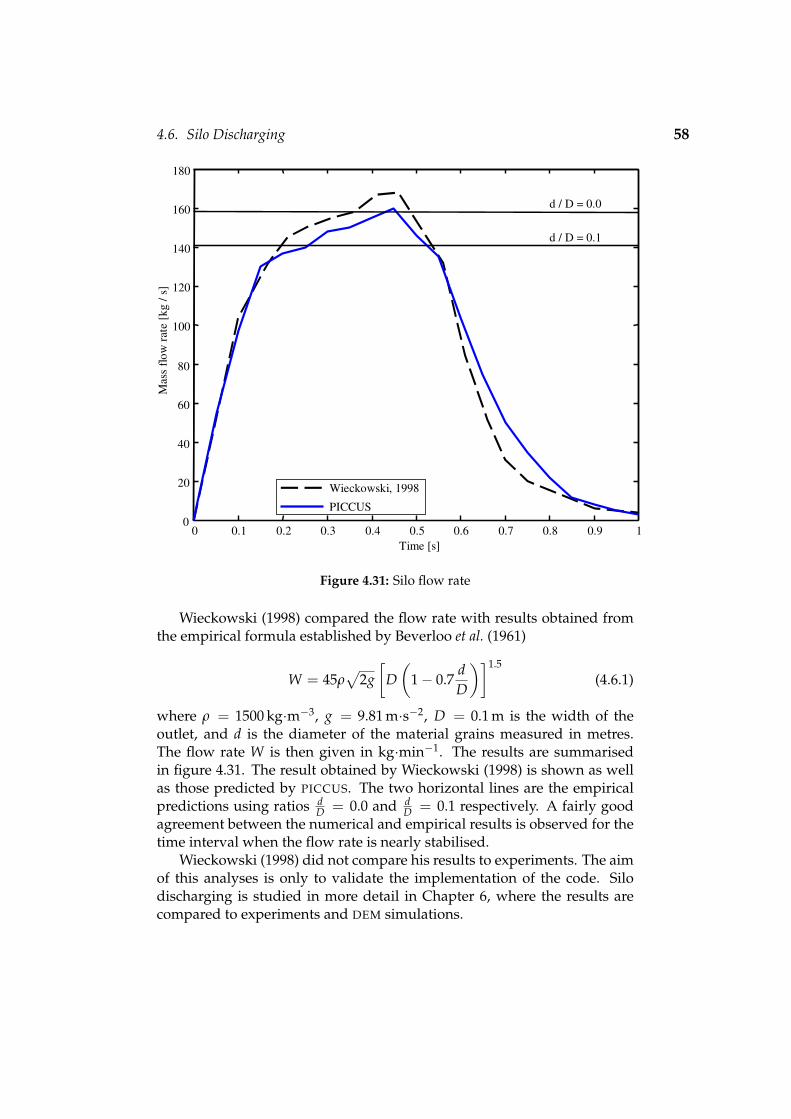
4.6. Silo Discharging 58
0 0.1 0.2 0.3 0.4 0.5 0.6 0.7 0.8 0.9 10
20
40
60
80
100
120
140
160
180
Time [s]
Mas
s flo
w ra
te [k
g / s
]
d / D = 0.1
d / D = 0.0
Wieckowski, 1998
PICCUS
Figure 4.31: Silo flow rate
Wieckowski (1998) compared the flow rate with results obtained fromthe empirical formula established by Beverloo et al. (1961)
W = 45ρ√
2g[
D(
1− 0.7dD
)]1.5
(4.6.1)
where ρ = 1500 kg·m−3, g = 9.81 m·s−2, D = 0.1 m is the width of theoutlet, and d is the diameter of the material grains measured in metres.The flow rate W is then given in kg·min−1. The results are summarisedin figure 4.31. The result obtained by Wieckowski (1998) is shown as wellas those predicted by PICCUS. The two horizontal lines are the empiricalpredictions using ratios d
D = 0.0 and dD = 0.1 respectively. A fairly good
agreement between the numerical and empirical results is observed for thetime interval when the flow rate is nearly stabilised.
Wieckowski (1998) did not compare his results to experiments. The aimof this analyses is only to validate the implementation of the code. Silodischarging is studied in more detail in Chapter 6, where the results arecompared to experiments and DEM simulations.
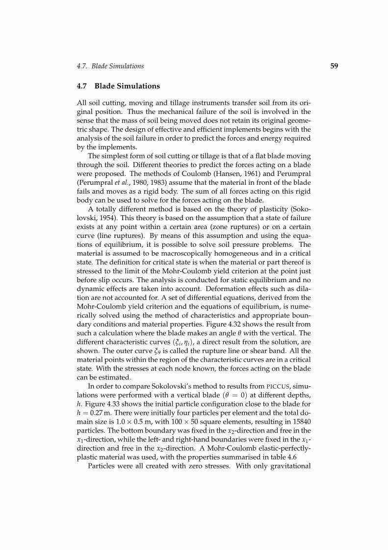
4.7. Blade Simulations 59
4.7 Blade Simulations
All soil cutting, moving and tillage instruments transfer soil from its ori-ginal position. Thus the mechanical failure of the soil is involved in thesense that the mass of soil being moved does not retain its original geome-tric shape. The design of effective and efficient implements begins with theanalysis of the soil failure in order to predict the forces and energy requiredby the implements.
The simplest form of soil cutting or tillage is that of a flat blade movingthrough the soil. Different theories to predict the forces acting on a bladewere proposed. The methods of Coulomb (Hansen, 1961) and Perumpral(Perumpral et al., 1980, 1983) assume that the material in front of the bladefails and moves as a rigid body. The sum of all forces acting on this rigidbody can be used to solve for the forces acting on the blade.
A totally different method is based on the theory of plasticity (Soko-lovski, 1954). This theory is based on the assumption that a state of failureexists at any point within a certain area (zone ruptures) or on a certaincurve (line ruptures). By means of this assumption and using the equa-tions of equilibrium, it is possible to solve soil pressure problems. Thematerial is assumed to be macroscopically homogeneous and in a criticalstate. The definition for critical state is when the material or part thereof isstressed to the limit of the Mohr-Coulomb yield criterion at the point justbefore slip occurs. The analysis is conducted for static equilibrium and nodynamic effects are taken into account. Deformation effects such as dila-tion are not accounted for. A set of differential equations, derived from theMohr-Coulomb yield criterion and the equations of equilibrium, is nume-rically solved using the method of characteristics and appropriate boun-dary conditions and material properties. Figure 4.32 shows the result fromsuch a calculation where the blade makes an angle θ with the vertical. Thedifferent characteristic curves (ξi, ηi), a direct result from the solution, areshown. The outer curve ξ9 is called the rupture line or shear band. All thematerial points within the region of the characteristic curves are in a criticalstate. With the stresses at each node known, the forces acting on the bladecan be estimated.
In order to compare Sokolovski’s method to results from PICCUS, simu-lations were performed with a vertical blade (θ = 0) at different depths,h. Figure 4.33 shows the initial particle configuration close to the blade forh = 0.27 m. There were initially four particles per element and the total do-main size is 1.0× 0.5 m, with 100× 50 square elements, resulting in 15840particles. The bottom boundary was fixed in the x2-direction and free in thex1-direction, while the left- and right-hand boundaries were fixed in the x1-direction and free in the x2-direction. A Mohr-Coulomb elastic-perfectly-plastic material was used, with the properties summarised in table 4.6
Particles were all created with zero stresses. With only gravitational

4.7. Blade Simulations 60
0.2 0.4 0.6 0.8 1
-0.4
-0.2
0 η0
η22
ξ9ξ8ξ7
ξ6ξ5ξ4ξ3ξ2ξ0ξ1
x1
x2
η1η2
η3η4
η5η6
η7η8
η9η10η11η12η13η14η16η18η20
θ
Figure 4.32: Blade forces - sample calculation
Material
Bla
de
Figure 4.33: Initial particle configuration close to the blade, h = 0.27 m

4.7. Blade Simulations 61
Table 4.6: Material properties used in blade simulation
Name Symbol Value
Young’s modulus E 1 GPa
Density ρ 1500 kg·m−3
Poisson’s ratio ν 0.3
Friction angle φ 35
Dilatancy angle ψ 0
Cohesion c 0 Pa
Tensile limit σt 0 Pa
Table 4.7: Blade simulation parameters
Name Symbol Value
Integration time step ∆t 1× 10⁻⁵ s
Damping α 0
Gravity gi (0.00,−9.81) m·s−2
Blade-material friction µ 0.2
Blade velocity v 0.005 m·s−1
forces acting on the material, and using a damping constant of α = 0.8,the material was then allowed to reach static equilibrium. Equilibrium wasdefined when the maximum value in particle velocity satisfied |vmax
i | ≤1× 10⁻⁸m·s−1.The stresses at static equilibrium are shown in figure 4.34. Using the simu-lation parameters summarised in table 4.7, the blade was given a constantvelocity in the x1-direction. This resulted in the material in front of theblade being pushed forward until it yielded. Figure 4.35 shows the x1- andx2-forces exerted by the blade on the material during a typical simulation.The negative x2-force indicates that the material tended to push the bladeupwards, out of the material.
The blade forces start from almost zero and then increase in value as thematerial is being accelerated. After 1.5 s the forces seem to reach a steadyvalue and only small oscillations are present. The average force between2.0 and 7.0 s was compared to the forces predicted by Sokolvski’s method.Figure 4.36 shows the results from using different blade depths. From thisit can be seen that there is good agreement between the two different me-thods. PICCUS’s predictions of the x1-force are roughly between 64 and

4.7. Blade Simulations 62
Figure 4.34: Blade simulation: initial stresses, h = 0.27 m
103 N too high, while there is excellent agreement on the x2-force. The per-centage difference, defined as
∆F% =F PICCUS − F Sokolovski
F Sokolovski 100% (4.7.1)
is shown in figure 4.37. From this it can be seen that as the blade depthincreases, the difference decreases.
The material failure can be investigated by looking at the velocity of theparticles. The Coulomb and Perumpral methods assume that the materialwithin the yield region moves as a rigid body with a definite shear bandseparating it from the virgin material. Figure 4.38 shows the velocity vec-tor of every tenth particle and the shear band calculated by Sokolovski’smethod. It is clear that the material points above the shear band have amuch higher velocity then the material points below the line.

4.7. Blade Simulations 63
0 1 2 3 4 5 6-1000
-500
0
500
1000
1500
2000
2500
3000
3500
4000
Time [s]
Forc
e [N
]
x1-force
x2-force
Figure 4.35: Blade simulation: typical blade forces, h = 0.21 m
The material failure can also be investigated by looking at which ma-terial points are stressed up to the Mohr-Coulomb yield surface f s = 0.Figure 4.39 and figure 4.40 show the material as well as the Sokolovski pre-dicted shear bands for h = 0.27 m and 0.15 m respectively. The material iscoloured according to the stress at each point. The lighter regions indicatematerial points with the stresses on the yield surface, i.e., material yieldingat that time, and the darker regions indicate material with stresses suchthat f s > 0, i.e., in an elastic state of stress. These figures also indicate goodagreement between the Sokolovski predictions and those obtained usingPICCUS. The material in the shear band and above it yields, while the ma-terial below the shear band stays in the elastic range. No cohesion was usedwhich means that the apex of the yield surface is at σ1 = σ2 = σ3 = 0. Thematerial at the free surface has stress components close to zero and there-fore it shows yielding even away from the region affected by the blade.
Different mesh sizes were used to investigate the effect of mesh refi-nement on the blade forces. A blade depth h = 0.21 m was used. Fi-gure 4.41 shows that the forces acting on the blade converge with meshrefinement. The effect of mesh refinement on the shear bands are shown inChapter 6, where polar and nonpolar results are compared to experiments,
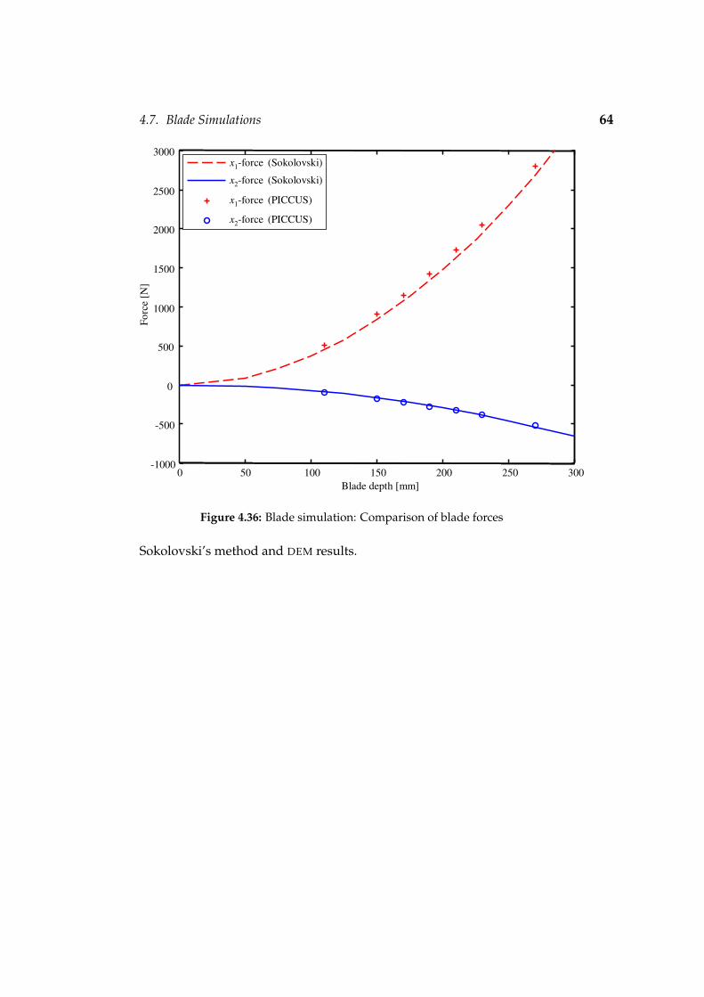
4.7. Blade Simulations 64
0 50 100 150 200 250 300-1000
-500
0
500
1000
1500
2000
2500
3000
Blade depth [mm]
Forc
e [N
]
x1-force (Sokolovski)
x2-force (Sokolovski)
x1-force (PICCUS)
x2-force (PICCUS)
Figure 4.36: Blade simulation: Comparison of blade forces
Sokolovski’s method and DEM results.

4.7. Blade Simulations 65
0.1 0.15 0.2 0.25 0.3-4
-2
0
2
4
6
8
10
12
14
16
Blade depth [mm]
Diff
eren
ce [%
]
x1-force
x2-force
Figure 4.37: Blade simulation: Percentage difference in the prediction of the bladeforces
Figure 4.38: Blade simulation: Particle velocity vectors, scaled 15 times, h = 0.27 m

4.7. Blade Simulations 66
Figure 4.39: Blade simulation: Material stress, lighter regions - material yielding,darker regions - material in an elastic state, h = 0.27 m
Figure 4.40: Blade simulation: Material stress, lighter regions - material yielding,darker regions - material in an elastic state, h = 0.15 m

4.7. Blade Simulations 67
0 1000 2000 3000 4000 5000 6000 7000 8000-500
0
500
1000
1500
2000
2500
Number of Elements [#]
Forc
e [N
]
80 × 40
40 × 20
100 × 50 120 × 60Sokolovski: x1-force
Sokolovski: x2-force
PICCUS: x1-force
PICCUS: x2-force
Figure 4.41: The effect of the mesh size on the blade forces, h = 0.21 m

4.8. Elastic Strip Footing 68
4.8 Elastic Strip Footing
This analysis concerns a strip loading on an elastic mass. Figure 4.42 showsthe geometry of the problem being analysed and the PICCUS discritisation.Only one symmetric half of the problem is analysed with the boundaryconditions as shown in the figure. A square mesh of 80× 80 elements isutilised with a smooth interface between the rigid footing and the material.The elastic material properties are summarised in table 4.8.
1 m
25 m
25 m
x 1-c
onst
rain
ed
x1-x2 - constrained
Sym
met
ry:x
1-c
onst
rain
ed
Figure 4.42: PICCUS model for strip loading on an elastic mass
The footing was given a downward velocity of V = 0.01 mm·s−1 until thepressure reached a 100 kPa. The footing was then kept still and a dampingfactor of α = 0.8 was applied until a equilibrium state was reached.

4.8. Elastic Strip Footing 69
Table 4.8: Material properties used in elastic footing simulation
Name Symbol Value
Young’s modulus E 20 GPa
Density ρ 1000 kg·m−3
Poisson’s ratio ν 0.2
2b
P
x1
x2(x1,x2)
Figure 4.43: Definition of parameters used in the elastic solution to the footingproblem
A closed-form solution for this problem, using the notation given in fi-gure 4.43, is given by Poulos & Davis (1974). The stresses at the coordinates(x1x2) under the surface are given by
σ11 =Pπ
[β− sinβ cos(β + 2δ)]
σ22 =Pπ
[β + sinβ cos(β + 2δ)]
τ12 =Pπ
sinβ sin(β + 2δ)
(4.8.1)
and the principal stresses are
σ1 =Pπ
(β + sinβ)
σ2 =Pπ
(β− sinβ)
τmax =Pπ
sinβ
(4.8.2)
Figure 4.44 shows the principal stresses along x1 = 0 under the strip foo-
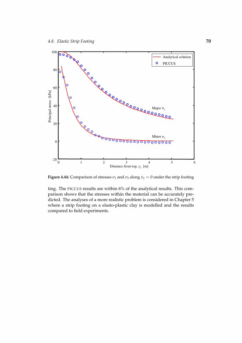
4.8. Elastic Strip Footing 70
0 1 2 3 4 5 6-20
0
20
40
60
80
100
Distance from top, x2 [m]
Prin
cipa
l str
ess
[kPa
]
Major
1
Minor
3
Analytical solution
PICCUS
Figure 4.44: Comparison of stresses σ1 and σ3 along x1 = 0 under the strip footing
ting. The PICCUS results are within 6% of the analytical results. This com-parison shows that the stresses within the material can be accurately pre-dicted. The analyses of a more realistic problem is considered in Chapter 5where a strip footing on a elasto-plastic clay is modelled and the resultscompared to field experiments.

Chapter 5
Experimental Validation
5.1 Introduction
In the previous chapter analytical solutions and published numerical re-sults were used to validate PICCUS. In this chapter published experimentaldata is used for validation.
5.2 Anchor Plates in Sand
Anchors form an important component of many civil engineering projects.Anchors are typically used to support other structures such as towers, bridgesand roofs. Rowe & Davis (1982a,b), review the methods used to model andanalyse anchor behaviour.
The prediction of anchor plate behaviour is usually restricted to the li-miting conditions of elastic displacement or ultimate capacity. The elasticanalysis only yields a load-displacement response within the elastic range.Many approaches have been given to estimate the ultimate capacity or col-lapse load. These methods involve the use of limit equilibrium concepts,the method of characteristics and empirical corrections.
In general, anchor behaviour is influenced by the material properties,the initial stress state, the boundary conditions and the anchor roughness(Rowe and Davis, 1982b). As validation, the passive resistance of rectan-gular anchors embedded in sand is modelled. The results are comparedto experimental results, under the assumption of plane strain. Verticallypulled anchors and anchors pulled upwards at an angle of 45 are investi-gated.
5.2.1 Vertically Pulled Anchors
Rowe & Davis (1982a) investigated the behaviour of vertically and hori-zontally pulled anchors in sand. Model tests were performed using a dry,medium grained quartz Sydney sand. The tests were performed in a steelbox 450 mm× 606 mm× 692 mm high, figure 5.1. The anchor was a 51 mmwide and 8 mm thick mild steel plate with length to breadth ratios of L
B =1, 2, 3, 4, 5, 8.75. All of the experimental load-displacement curves are notpublished, and only the results with a ratio of L
B = 8.75 were used forcomparisons. The load was applied to the centre of the anchor via a 8 mmdiameter rod at a constant velocity of 0.025 mm·s−1.
71

5.2. Anchor Plates in Sand 72
450
B = 518
140
h
V
Figure 5.1: Geometry for vertically pulled anchor. Dimensions are in mm.
The anchor plate was put on top of a 140 mm layer of sand in the bottomof the box. Additional sand was than added until the anchor was buried tothe required depth. The sand was sprinkled from a height of 25 mm abovethe surface. The unit weight of the sand γ was determined by weighingthe sand in the box and measuring the total volume occupied. Triaxial testswere performed to determine the friction and dilatancy angles. No attemptwas made to measure the K0 value of the sand in the box, but empiricalcorrelations were used to make an estimate. Poisson’s ratio was also esti-mated. The stiffness of the material is not given at all, and simulations wereperformed with different stiffness values.
Figure 5.2 shows the simulation model. A symmetry plane is used tomodel only half of the problem depicted in figure 5.1. The other boundaryconditions are shown in the figure. Initial stresses were specified usingK0 = 0.47. Damping (α = 0.8) was used to reach an equilibrium state, af-ter which the damping was removed and the anchor, modelled as a rigidbody, moved at constant velocity in the vertical x2-direction. The mate-rial properties and simulation parameters are summarised in table 5.1 andtable 5.2 respectively.
Two embedded ratios were used for comparison: hB = 3 and h
B = 5. Thedomain was divided into 44× 58 and 44× 78 square elements respectively,to model the different ratios. Figure 5.3 shows the load-displacement cur-ves for h
B = 3, stiffness values of E = 700 kN·m−2 and E = 1000 kN·m−2
and a rough and smooth sand-anchor interface. The higher stiffness valueof E = 1000 kN·m−2 clearly follows the experimental result more closelyin the initial elastic region. The difference between a rough and smoothinterface has no effect on the ultimate capacity, which is within 5% of the

5.2. Anchor Plates in Sand 73
x1-x2-fixed
x 1-f
ixed
x 1-f
ixed
(sy
mm
etry
)
Free surface
Figure 5.2: Simulation model for vertically pulled anchor.

5.2. Anchor Plates in Sand 74
Table 5.1: Mohr-Coulomb material data vertical anchor pull-out test
Description Symbol Value
Young’s modulus E 700 MPa / 1000 MPa
Poisson’s ratio ν 0.2
Unit weight γ 14.9 kN·m−3
Friction angle φ 32
Tensile limit σt 0 Pa
Dilatancy angle ψ 4
Cohesion c 0 Pa
Material-wall friction µwall Smooth/Rough
Coefficient of earth pressure K0 1− sin(φ) = 0.47
Table 5.2: Vertically pulled anchor simulation parameters
Name Symbol Value
Integration time step ∆t 1× 10⁻⁵ s
Damping α 0
Gravity gi (0.00,−9.81) m·s−2
Anchor velocity v 0.025 mm·s−1
Number of material points Np 10608 - 14303
Initial number of degrees-of-freedom DOF 5095
measured value. It is also observed by Rowe & Davis (1982a) that for verti-cally pulled anchors, the anchor roughness has little effect on the ultimatecapacity.Figure 5.4 shows the experimental and numerical results for h
B = 5. The an-chor is assumed to be smooth and the stiffness taken as E = 1000 kN·m−2.The simulation accurately predicts the load-displacement behaviour in theelastic region and over predicts the ultimate capacity by roughly 3%.
All of the above simulations were performed using a Mohr-Coulombconstitutive model with the parameters given in table 5.1. Figure 5.5 showsthe results using a Drucker-Prager model. The same friction and dilatancyangles were used, and the Drucker-Prager parameters were chosen suchthat the yield surface fits within the Mohr-Coulomb yield surface (inneradjustment, equation H.6.2). Using the Drucker-Prager model, there is aslightly more gradual transition from the elastic state to the plastic state.
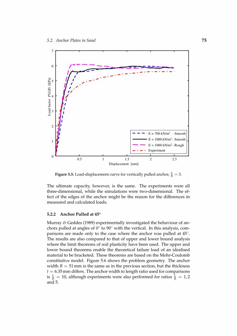
5.2. Anchor Plates in Sand 75
0.5 1 1.5 2 2.50
1
2
3
4
5
6
7Lo
ad fa
ctor
P/(
LB)
[kPa
]
Displacement [mm]
E = 700 kN/m2 - Smooth
E = 1000 kN/m2 - Smooth
E = 1000 kN/m2 - Rough Experiment
Figure 5.3: Load-displacement curve for vertically pulled anchor, hB = 3.
The ultimate capacity, however, is the same. The experiments were allthree-dimensional, while the simulations were two-dimensional. The ef-fect of the edges of the anchor might be the reason for the differences inmeasured and calculated loads.
5.2.2 Anchor Pulled at 45°
Murray & Geddes (1989) experimentally investigated the behaviour of an-chors pulled at angles of 0 to 90 with the vertical. In this analysis, com-parisons are made only to the case where the anchor was pulled at 45.The results are also compared to that of upper and lower bound analysiswhere the limit theorems of soil plasticity have been used. The upper andlower bound theorems enable the theoretical failure load of an idealisedmaterial to be bracketed. These theorems are based on the Mohr-Coulombconstitutive model. Figure 5.6 shows the problem geometry. The anchorwidth B = 51 mm is the same as in the previous section, but the thicknesst = 6.35 mm differs. The anchor width to length ratio used for comparisonsis L
B = 10, although experiments were also performed for ratios LB = 1, 2
and 5.

5.2. Anchor Plates in Sand 76
1 2 3 4 5 60
5
10
15Lo
ad fa
ctor
P/(
LB)
[kPa
]
Displacement [mm]
E = 1000 kN/m2 - Smooth
Experiment
Figure 5.4: Load-displacement curve for vertically pulled anchor, hB = 5.
A medium grained sand, known as Portishead Fines, was compactedin layers by vibration with the anchor fixed in position in the test contai-ner. The sand in the container was weighed to calculate the average unitweight γ. Direct shear box tests on the sand yielded the friction angle φand cohesion c. A modified shear box was used to determine the interfacefriction µwall . No attempt has been made to determine the material stiff-ness E, Poisson’s ratio ν, the dilatancy angle ψ or the coefficient at rest K0.It has, however been shown in the previous section that the stiffness haslittle effect on the limit load. Poisson’s ratio is taken to be ν = 0.2 and Mur-ray & Geddes (1989) estimated the dilatancy angle to be within the rangeψ = 5 − 12. Table 5.3 summarises the material properties. Figure 5.7shows the PICCUS model and table 5.4 summarises the simulation parame-ters. The domain was divided into 80 × 32, 80 × 45 and 80 × 59 squareelements for the different embedded ratios h
B = 2, 4 and 6.Murray & Geddes (1989) do not provide the load-displacement curves
obtained from their experiments, but only give the ultimate loads for diffe-rent embedded depths. The definition given by Rowe & Davis (1982a,b) isused to determine the ultimate capacity, given a load-displacement curve.The kn failure load is defined as the load which produces n times the dis-
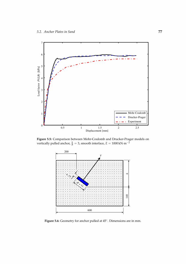
5.2. Anchor Plates in Sand 77
0.5 1 1.5 2 2.50
1
2
3
4
5
6
7
Load
fact
or P
/(LB
) [k
Pa]
Displacement [mm]
Mohr-Coulomb
Drucker-PragerExperiment
Figure 5.5: Comparison between Mohr-Coulomb and Drucker-Prager models onvertically pulled anchor, h
B = 3, smooth interface, E = 1000 kN·m−2
600
140
h
B = 51
6.35
V200
Figure 5.6: Geometry for anchor pulled at 45. Dimensions are in mm.

5.2. Anchor Plates in Sand 78
Table 5.3: Mohr-Coulomb material data for 45° anchor pull-out
Description Symbol Value
Young’s modulus E 1500 MPa
Poisson’s ratio ν 0.2
Unit weight γ 16.8 kN·m−3
Friction angle φ 44
Tensile limit σt 0 Pa
Dilatancy angle ψ 12
Cohesion c 0 Pa
Anchor-sand friction µwall 11, (0.19)
Coefficient of earth pressure K0 1− sin(φ) = 0.31
Figure 5.7: Computed Geometry for anchor pulled at 45.
Table 5.4: Anchor pulled at 45° simulation parameters
Name Symbol Value
Integration time step ∆t 1× 10⁻⁵ s
Damping α 0
Gravity gi (0.00,−9.81) m·s−2
Anchor velocity v 0.012 mm·s−1
Number of material points Np 10221 - 19021
Initial number of degrees-of-freedom DOF 5120 - 9602

5.2. Anchor Plates in Sand 79
0.2 0.4 0.6 0.8 1 1.2 1.4 1.6 1.80
0.5
1
1.5
2
2.5
3
Displacement [mm]
Load
fact
or,
P/(
Ah)
[-]
E
1
(n-1)
Failure load
Figure 5.8: Load-displacement curve for anchor pulled at 45°, hB = 2.
placement that would have occurred had the soil remained elastic. Thisdefinition is not dependent on scale or stiffness modulus, but the value ofn remains arbitrary. Rowe & Davis (1982a,b) suggest a value n = 4, i.e., k4failure load. Figure 5.8 plots the dimensionless load factor P/γAh againstthe anchor displacement. P is the load on the anchor measured in N, γ theunit weight, A = BL is the frontal area of the anchor and h the embeddeddepth. The calculation of the kn failure load is also shown by the figure.The ultimate failure loads at different depth ratios are plotted in figure 5.9.The simulations under predict the measured ultimate capacity for all threedepth ratios. The maximum difference is 9.3%. The upper-bound limit isalso shown. The biggest unknown in this problem is the initial stress state.The value of K0 has been taken to be 1− sin(φ) according to Jaky (1944).The way of preparing the sand bed, however, will have an influence onthis value. Rowe & Davis (1982a) have shown, that for a particular case, anincrease in K0 from 0.5 to 1.0, caused a 6% increase in the ultimate capacity.
The results show that PICCUS can model anchor pull-out tests which isdifficult to model with FEM. Special FEM contact elements would be nee-ded to model the interface between the soil and the anchor. The contactelements should be able to model break-away of the soil behind the an-
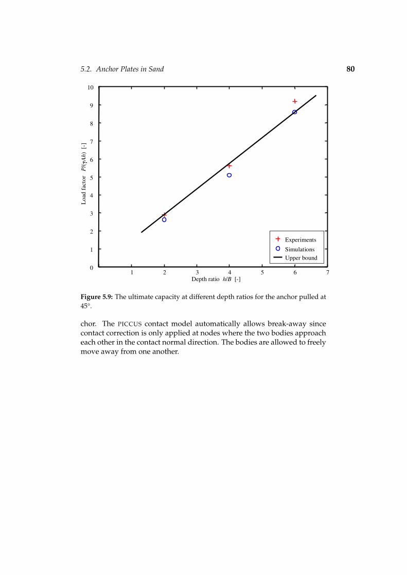
5.2. Anchor Plates in Sand 80
1 2 3 4 5 6 70
1
2
3
4
5
6
7
8
9
10
Depth ratio h/B [-]
Load
fact
or
P/(
Ah)
[-]
Experiments
SimulationsUpper bound
Figure 5.9: The ultimate capacity at different depth ratios for the anchor pulled at45°.
chor. The PICCUS contact model automatically allows break-away sincecontact correction is only applied at nodes where the two bodies approacheach other in the contact normal direction. The bodies are allowed to freelymove away from one another.

5.3. Strip Footings 81
5.3 Strip Footings
In this section two strip footing problems are analysed: the one being aslope stability problem (vertical cut) and the other a bearing capacity pro-blem. Rilling (1994) performed well documented large-scale field tests un-der plane strain conditions. PICCUS results are compared to the experimen-tal results, as well as to the results from PLAXIS. PLAXIS (PLAXIS, 2 June2003) is a quasi-static finite element code based on implicit integration ofthe differential constitutive law. The PLAXIS simulations were performedby the Institute of Geotechnical Engineering at the University of Stuttgart.
5.3.1 Test Setup
The frame depicted in figure 5.10 was used to perform tests under planestrain conditions. In order to ensure plane strain on a middle section, thestrip footing was divided into three parts; the outer parts were one metrelong and the middle part 0.4 metre. Measurements were only done on themiddle section. The sections were placed close together, but without con-tact. The loading was controlled by hydraulic presses and in such a waythat all three sections had the same vertical displacements. With measure-ments made only on the middle section, plane strain conditions (measure-ments) can be assumed.
Figure 5.11 shows typically measured load-settlement curves. This graphclearly indicates the different stress levels present in the two different pro-blems being analysed. During the slope stability test, test A, the loadingpressure is in the order of 150 kPa, while during the bearing capacity test,tests B1 and B2, it is in the order of 800 kPa − 1000 kPa. The differencebetween the two B-tests, B1 and B2, is due to different locations and soilheterogeneity.Although both tests involve plane strain strip footings on the same type ofsoil, they are completely different. The footing near the vertical cut invol-ves a collapse mechanism as considered in slope stability analyses and theother one yields a Prandl-type failure. This is also reflected in the magni-tudes of the collapse loads, being very low for the slope-type failure andhigh for the usual bearing capacity problem. Considering these differentstress levels and different collapse mechanisms, these field model tests areoutstanding for validating numerical collapse load calculations. Numericalcollapse load analyses are not directly needed for simple situations such asa footing on a homogeneous half space, as this bearing capacity problemhas been solved analytically, but it is essential for more complex problems,e.g. for a footing near a slope as also considered in this study.
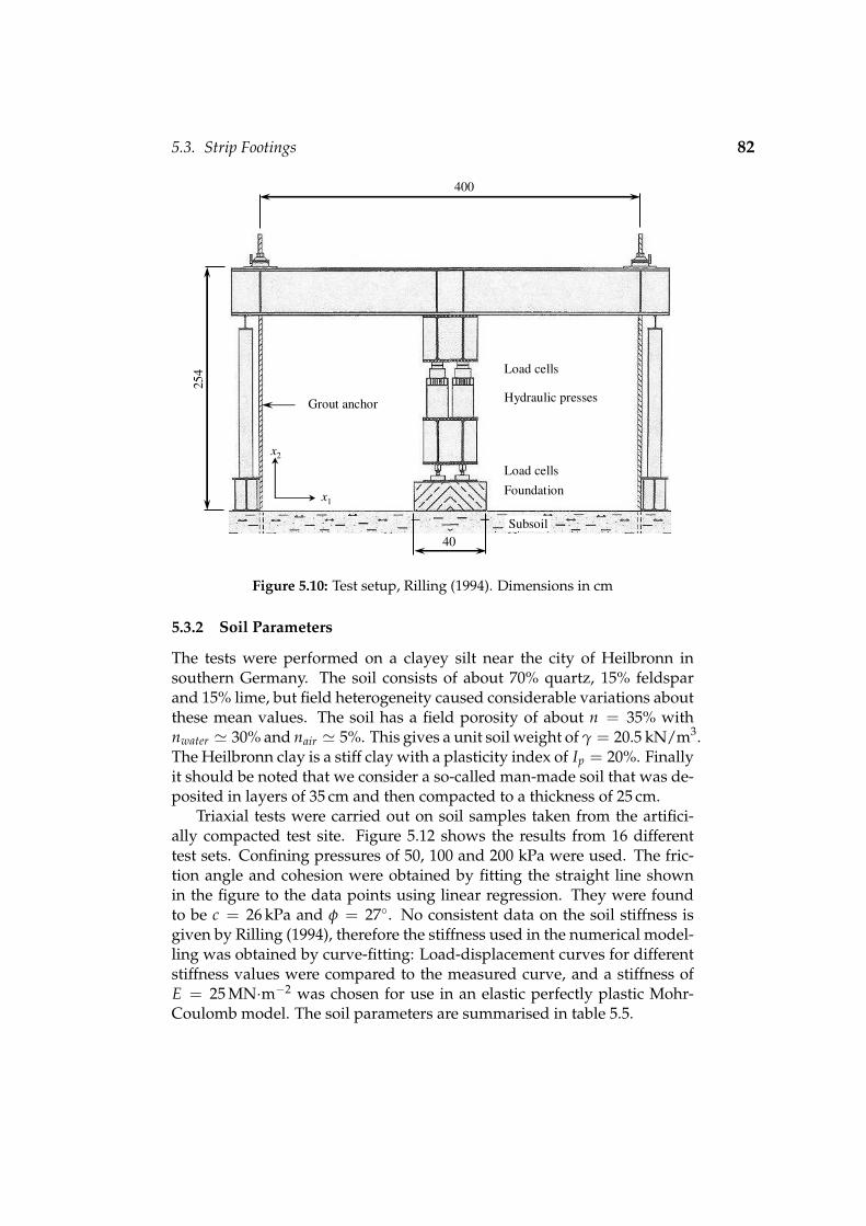
5.3. Strip Footings 82
x1
x2
40025
4
Grout anchor
Load cells
Hydraulic presses
Load cellsFoundation
Subsoil40
Figure 5.10: Test setup, Rilling (1994). Dimensions in cm
5.3.2 Soil Parameters
The tests were performed on a clayey silt near the city of Heilbronn insouthern Germany. The soil consists of about 70% quartz, 15% feldsparand 15% lime, but field heterogeneity caused considerable variations aboutthese mean values. The soil has a field porosity of about n = 35% withnwater ' 30% and nair ' 5%. This gives a unit soil weight of γ = 20.5 kN/m3.The Heilbronn clay is a stiff clay with a plasticity index of Ip = 20%. Finallyit should be noted that we consider a so-called man-made soil that was de-posited in layers of 35 cm and then compacted to a thickness of 25 cm.
Triaxial tests were carried out on soil samples taken from the artifici-ally compacted test site. Figure 5.12 shows the results from 16 differenttest sets. Confining pressures of 50, 100 and 200 kPa were used. The fric-tion angle and cohesion were obtained by fitting the straight line shownin the figure to the data points using linear regression. They were foundto be c = 26 kPa and φ = 27. No consistent data on the soil stiffness isgiven by Rilling (1994), therefore the stiffness used in the numerical model-ling was obtained by curve-fitting: Load-displacement curves for differentstiffness values were compared to the measured curve, and a stiffness ofE = 25 MN·m−2 was chosen for use in an elastic perfectly plastic Mohr-Coulomb model. The soil parameters are summarised in table 5.5.
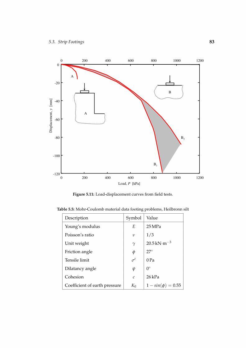
5.3. Strip Footings 83
0 200 400 600 800 1000 1200-120
-100
-80
-60
-40
-20
0
Load, P [kPa]
Dis
plac
emen
t, y
[mm
]
A
B
A
B1
B2
0 200 400 600 800 1000 1200
Figure 5.11: Load-displacement curves from field tests.
Table 5.5: Mohr-Coulomb material data footing problems, Heilbronn silt
Description Symbol Value
Young’s modulus E 25 MPa
Poisson’s ratio ν 1/3
Unit weight γ 20.5 kN·m−3
Friction angle φ 27
Tensile limit σt 0 Pa
Dilatancy angle ψ 0
Cohesion c 26 kPa
Coefficient of earth pressure K0 1− sin(φ) = 0.55

5.3. Strip Footings 84
0 50 100 150 200 250 300 350 4000
50
100
150
200
250
300
350
400
450
500
p = (σ1 + σ2 + σ3 ) / 3 [kPa]
q=
(σ1
-σ3
) [k
Pa]
φ = 27°
c = 26 kPa
Figure 5.12: Triaxial results for Heilbronn silt
5.3.3 Bearing Capacity
Figure 5.13 shows the geometry used to model the bearing capacity pro-blem. In the case of PICCUS, the material points are also shown. In PLAXIS
a total of 1050 6-noded elements were used with 2171 nodes. In PICCUS aregular grid of 45× 30 = 1350 square 4-noded elements was used with atotal of 1426 nodes. Despite the comparable number of nodes the PICCUS-grid is finer than the PLAXIS mesh, as the PICCUS-analysis was carried outfor half a symmetric footing. The side boundaries were assumed smooth,i.e., only constrained in the horizontal direction. The bottom boundary wasconstrained in both the horizontal and vertical directions. A Ko = 1− sinφinitial stress state was assumed.
Table 5.6 shows the parameters used to perform the bearing capacity si-mulations. Figure 5.14 shows the load-displacement curves obtained fromfield measurements, PICCUS and PLAXIS. There is a good correspondencebetween the PICCUS and PLAXIS results, predicting failure loads of 692 and668 kPa respectively. The numerical methods accurately predict the mea-sured initial stiffness and correspond well to the field data up to the stagewhere the predicted failure loads are reached. The failure load, however,is underestimated by approximately 25%. This difference might be due to
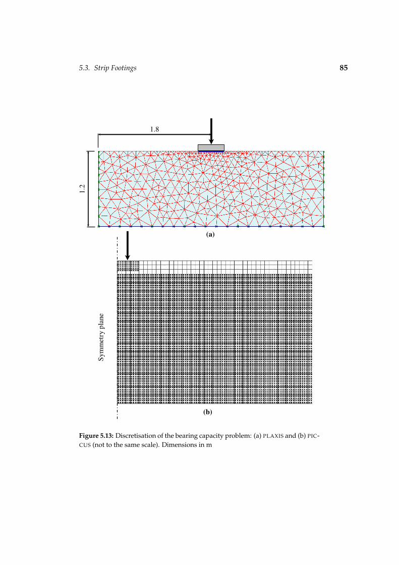
5.3. Strip Footings 85
1.8
1.2
(a)
(b)
Sym
met
ry p
lane
Figure 5.13: Discretisation of the bearing capacity problem: (a) PLAXIS and (b) PIC-CUS (not to the same scale). Dimensions in m
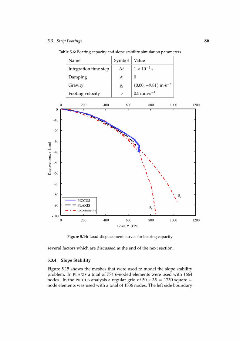
5.3. Strip Footings 86
Table 5.6: Bearing capacity and slope stability simulation parameters
Name Symbol Value
Integration time step ∆t 1× 10⁻⁵ s
Damping α 0
Gravity gi (0.00,−9.81) m·s−2
Footing velocity v 0.5 mm·s−1
0 200 400 600 800 1000 1200-100
-90
-80
-70
-60
-50
-40
-30
-20
-10
0
Load, P [kPa]
Dis
plac
emen
t, y
[mm
]
0 200 400 600 800 1000 1200
B1
B2
PICCUSPLAXISExperiments
Figure 5.14: Load-displacement curves for bearing capacity
several factors which are discussed at the end of the next section.
5.3.4 Slope Stability
Figure 5.15 shows the meshes that were used to model the slope stabilityproblem. In PLAXIS a total of 774 6-noded elements were used with 1664nodes. In the PICCUS analysis a regular grid of 50× 35 = 1750 square 4-node elements was used with a total of 1836 nodes. The left side boundary

5.3. Strip Footings 87
2.8
(a)
4.0
(b)
2.0
0.6 2.0
Figure 5.15: Discretisation of the slope stability problem: (a) PLAXIS and (b) PIC-CUS. Dimensions in m

5.3. Strip Footings 88
0 25 50 75 100 125 150-18
-16
-14
-12
-10
-8
-6
-4
-2
0
Load, P [kPa]
Dis
plac
emen
t, y
[mm
]0 25 50 75 100 125 150
PICCUSPLAXISExperiment
Figure 5.16: Load-displacement curves for slope stability
was assumed smooth, i.e., only constrained in the horizontal direction. Thebottom boundary was constrained in both the horizontal and vertical direc-tions. The initial stress state was generated by first creating material overthe whole domain, using K0 = 1 − sinφ. The vertical cut was than ge-nerated by removing the material layer by layer. After each removal, thematerial was allowed to deform and to reach static equilibrium. The si-mulation parameters are summarised in table 5.6. Figure 5.16 shows theload-displacement curves for this problem. The PICCUS and PLAXIS resultsare in good agreement, but underestimate the failure load by roughly 30%.
5.3.5 Conclusions
The results lead to the conclusions that PICCUS produces results that coin-cide with the results from a conventional nonlinear elasto-plastic finite ele-ment method. Another observation is that the failure load is significantlyunderestimated by both numerical analyses. In order to understand thisone might consider the analytical solution of Soil Mechanics text books for

5.3. Strip Footings 89
the bearing capacity, which reads
Pmax = c Nc + γ b Nb (5.3.1)
where b is the footing width and
Nc =Nd − 1tanφ
Nb = (Nd − 1)tanφ
Nd =1 + sinφ
1− sinφeπtanφ
(5.3.2)
Using the triaxial friction angle, φtr = 27, the ultimate capacity is calcula-ted Pmax = 674 kPa. The value of 674 kPa corresponds well to the numericalresults, but not to the measured values. In order to match the latter values,one would have to use a plane strain friction angle of φps = 30 whichwould yield Pmax = 946 kPa. The friction angle φtr = 27 has been deter-mined from triaxial experiments and used here in plane strain modelling.The ratio between the triaxial- and plane strain friction angle is φps
φtr= 1.1.
For cohesive soils, this ratio of 1.1 is also suggested by Kulhawy & Mayne(1990), whilst Wroth (1984) suggested the very similar ratio of 9
8 = 1.125.Indeed, triaxial compression tests give relatively low friction angles andthe use of such values in computations is conservative. For geotechnicaldesign, it may be right to choose conservative values, but this would notresult in accurate predictions when numerical analyses are used to predictreality.

Chapter 6
Blade, Bucket and Silo Modelling
6.1 Introduction
In this chapter, the flow of granular material (corn and sand) in front of flatblades, into buckets and silo discharging are investigated. The blade andbucket modelling follows on that of Coetzee (2000) who performed two-dimensional DEM simulations and compared the results to experimentswith corn. In this study, PICCUS results of blades and buckets are com-pared to both the DEM and experimental results of Coetzee (2000). PICCUS
and DEM results of silo discharging are compared to experiments with cornand sand which were done as part of this study. Polar and nonpolar conti-nua are used. The blade and the bucket are modelled as rigid bodies, whilethe corn and sand are modelled with Drucker-Prager and Mohr-Coulombtheories.
6.2 Blade and Bucket Modelling
6.2.1 Two-dimensional Test Rig
Figure 6.1 shows the main components of the test rig. Two glass panels,2200× 820 mm are mounted on the base structure. The distance betweenthese two panels is about 200 mm and is slightly adjustable to ensure thatthe tool profile is lined up between the two panels. The one panel (view-ing side) consists of two glass sheets, one 10 mm and one 6 mm thick. The10 mm glass is to resist the high lateral pressures created by the materialbeing pushed forward by the blade/bucket. The 6 mm glass sheet can ea-sily be replaced if it gets scratched. The other panel (non-viewing side) con-sists of a 3 mm steel sheet and a 6 mm glass sheet. The steel mainly resiststhe lateral pressure while the function of the glass is to have the friction onboth sides the same.
The profile is attached to the trolley via a four-bar linkage mechanism.The trolley is mounted on two sets of linear ball bearings. A stepper motorconnected to a ball screw moves the trolley forwards and backwards. Fi-gure 6.2 shows the use of the arm-mechanism. When ground-engagementtools such as dragline buckets are used, the bucket must have freedom ofmotion in both the vertical and lateral directions for three-dimensional si-mulations and at least freedom of motion in the vertical direction for two-dimensional simulations. The arm-mechanism allows freedom of motionin the vertical direction. Arm 1 is always fixed to the trolley, figure 6.2a,
90

6.2. Blade and Bucket Modelling 91
Blade /Bucket ProfileStrain Gauges
StepperMotor
Lifting Frame
TrolleyArm Mechanism
Glass Panels
Linear BearingsMotion
x2
x1O
Figure 6.1: Two-dimensional test rig, Coetzee (2000)
while arm 2 can move freely in the vertical direction, figure 6.2c. Counterweights can be added at the positions indicated, figure 6.2a. This allows theweight of the bucket to be changed and the weight of the arms and linkagesto be cancelled. For simulation of other ground-engagement tools such asbulldozer blades and cutting tools, arm 2 can be locked.
The whole test rig can be inclined with the use of the lifting frame. Thiscan be used to simulate the drag angle of draglines or any other tool wor-king on an incline. The test rig can be inclined in steps of 5° up to a maxi-mum of β = 30. When the test rig makes an angle β with the horizontal,the two vertical arms are also at an angle β to the vertical. This means thatthe freedom of motion is no longer in the vertical direction. To overcomethis problem arm 1 can be rotated relative to the trolley as in figure 6.2b.This ensures that arm 2 stays in a vertical position. Further, the angle of theprofile relative to vertical arm 2, i.e. the attack angle, can be changed sinceit is a parameter that influences the profile performance. The profiles arefitted with two teflon wipers, one on each side, to prevent particles frommoving between the profile and the glass. Three sets of strain gauges areused to measure the x1-force, x2-force and moment acting on the profile.The x1- and x2-directions are indicated in figure 6.1.
The blade in the experiments had a height of 350 mm and the bucketdimensions are shown in figure 6.3. The moment centre Om is the point atwhich the moment acting on the bucket is measured.

6.2. Blade and Bucket Modelling 92
Forces on Blade
Counter Weights
Ball Screw Force
Arm 1
Arm 2
(a)
Counter Weights
(b)
(c)
Figure 6.2: 2-D Test rig arm mechanism, Coetzee (2000)
6.2.2 Material
Rowlands (1991) observed that seed grains are suitable for experimentaltesting and closely resemble natural granular flow into dragline buckets.The grains have a relatively low friction coefficient with glass, which ma-kes it a perfect experimental material. The seed grains were also found sui-table for DEM simulations because the stiffness of the grains is less than thestiffness of, say, gravel. The smaller stiffness results in a larger time step,Coetzee (2000). For a close-packed assembly the stable time step is roughlyinversely proportional to the particle stiffness. Coetzee (2000) made use ofcorn and wheat grains. These two materials have very similar propertiesand in this study, only the results from using corn will be used (figure 6.4).
Oedometer and shear box tests were performed to determine the cornproperties. The oedometer tests yielded an oedometer stiffness Eoed. The
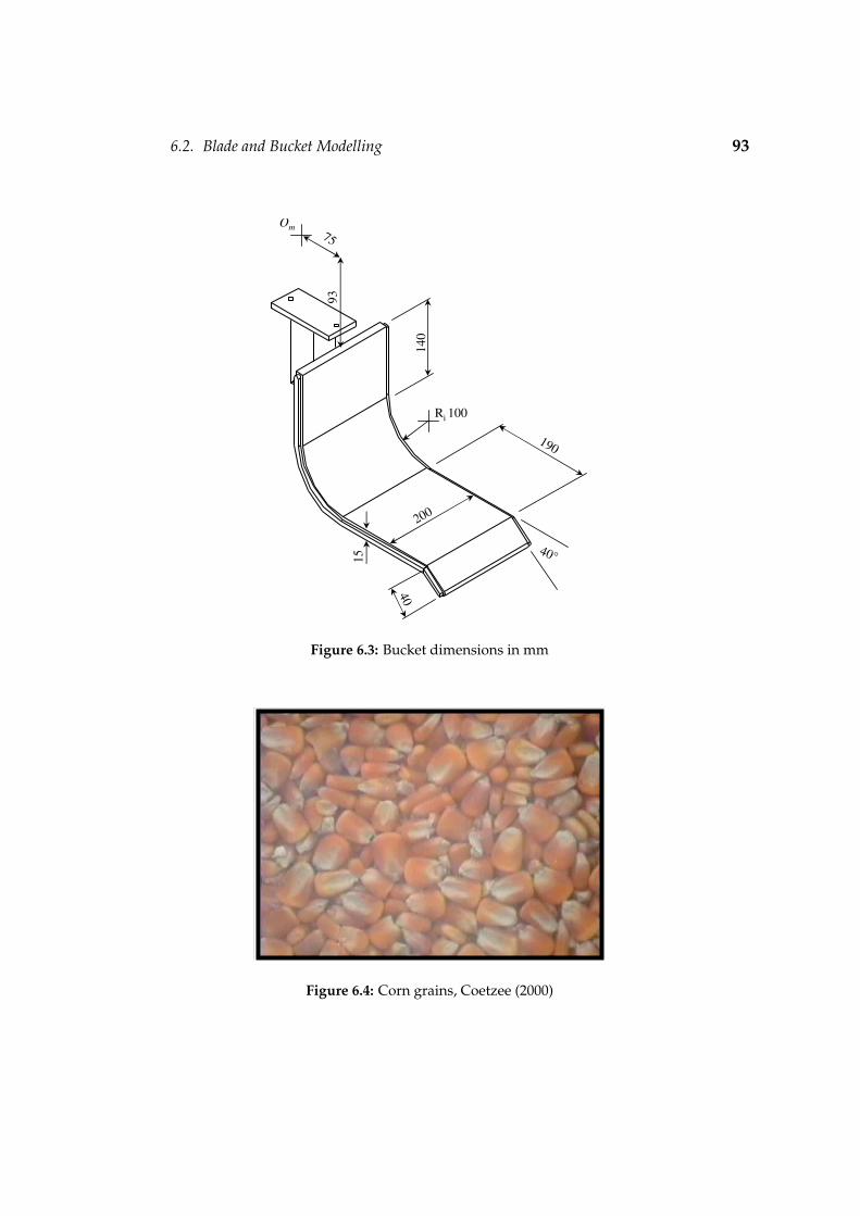
6.2. Blade and Bucket Modelling 93
140
93
75Om
Ri 100
190
200
40
40°15
Figure 6.3: Bucket dimensions in mm
Figure 6.4: Corn grains, Coetzee (2000)

6.2. Blade and Bucket Modelling 94
5 – 9
8 - 12 5 - 6
4 - 5
3 - 6
2.5 – 4.5
1.5 – 3.0
3 - 5
(a) (b)
Figure 6.5: Corn grains (a) measured [mm] (b) DEM grain, Coetzee (2000)
material stiffness or Young’s modulus E is related to the oedometer stiffnessby the following relation (Coetzee, 2000)
E = Eoed(1 + ν)(1− 2ν)
1− ν(6.2.1)
where ν is Poisson’s ratio. From the shear tests, the friction angle φ andcohesion c were determined. By replacing half of the shear box with a glassor steel sheet, the friction between corn and glass and corn and steel couldbe determined. Poisson’s ratio and the dilatancy angle were not measured.
6.2.3 DEM Simulations
Coetzee (2000) performed DEM simulations using the commercial code PFC2D
(Itasca, 1999). Figure 6.5 shows the range of the measured dimensions ofthe grains and the DEM particles used to model a single grain. A singleparticle consists of two circular particles rigidly joined to form a so-calledclump. The particle density, inter-particle friction coefficient and stiffnesswere determined through a series of numerical experiments. The particlesdensity was changed until the bulk density of an assembly of particles wasthe same as the measured value. To determine the inter-particle friction andstiffness, the oedometer and shear box experiments were repeated numeri-cally. The oedometer tests showed that the inter-particle friction had littleto no effect on the oedometer stiffness Eoed. Using different inter-particlestiffness’, the tests were repeated until the measured Eoed was obtained.The results showed that Eoed increases linearly with an increase in inter-particle stiffness. The friction angle calculated from the shear box resultswas influenced by both the inter-particle stiffness and friction. But, withthe stiffness known from the oedometer tests, only the friction coefficientswere changed until the measured friction angle was obtained.
Table 6.1 summarises the corn macro properties, and the micro proper-ties used in the DEM simulations. The macro properties were found to be

6.2. Blade and Bucket Modelling 95
Table 6.1: Corn material properties, Coetzee (2000)
Macro Properties Symbol Experiment DEM simulation
Young’s modulus E 2.76 MPa 1.84 MPa
Poisson’s ratio ν 0.2 -
Density ρ 778 kg·m−3 778 kg·m−3
Friction angle φ 26 24
Dilatancy angle ψ 2 -
Cohesion c 0 Pa 0 Pa
Tension cutoff σt 0 Pa -
Friction with glass φg 12 -
Friction with steel φs 14 14
Micro Properties Symbol Experiment DEM simulation
Particle stiffness kn = ks - 420 kN·m−1
Particle density ρp - 855 kg·m−3
Particle friction µ - 0.1
within the range measured by Reimbert & Reimbert (1976). Poisson’s ratiohas been estimated ν = 0.2 and the calculation of the dilatancy angle ψ willbe explained later.
6.2.4 Effect of Tool Velocity
Coetzee (2000) investigated the effect of blade velocity on the blade draftforce. The velocity could be varied continuously from 0 to 100 mm·s−1.Velocity changes within this range had no significant influence on the draftforce. This is in accordance with results from Albert et al. (1998) and Grissoet al. (1996), but Bohatier & Nouguier (2000), Siemens et al. (1965), Bagster& Bridgwater (1967) and Luth & Wismer (1971) showed that the draft forcedoes depend on the velocity. Bohatier & Nouguier (2000), Siemens et al.(1965) and Luth & Wismer (1971) observed a quadratic relation and Bagster& Bridgwater (1967) a linear relation at high velocities and independenceat low velocities. To summarise from the literature study, it seems thatthe tool forces are only significantly influenced at relatively high velocities(> 1 km·h−1). The shape of the tool and soil properties also were showedto have an influence. It is well known that the shear strength of soil isdependent on the shear rate, especially in soil with a high cohesion factor

6.2. Blade and Bucket Modelling 96
such as clay. For non-cohesive materials, the velocity has less of an effecton the tool forces.
6.2.5 Vertical Blade Modelling
The blade was given a constant velocity of 10 mm·s−1 during all experi-ments and simulations. The material was created layer-by-layer in the si-mulations, with the blade in position, and given an initial stress state assu-ming K0 = 1− sinφ. Using a damping coefficient of α = 0.8, the materialwas allowed to reach an equilibrium state under the influence of gravityalone. The two side boundaries were constraint in the x1-direction (hori-zontal) and in the polar case the horizontal and rotational directions. Thebottom boundary was fixed, i.e., constraint in both the horizontal and verti-cal directions and in the polar case the horizontal, vertical and rotational di-rections. No Cosserat rotation was allowed at the blade-material interfacewhich is true for a relatively smooth surface (Tejchman, 1997). Figure 6.6shows typical stresses at equilibrium. This is the same for the polar andnonpolar case, since in the polar case, all the couple stresses are zero.
Figure 6.7 and figure 6.8 show the flow of material in front of the bladeusing the nonpolar continuum. With only the dilatancy angle unknown,the simulation is repeated for three different values ψ = 2, 10 and ψ =φ = 26. The blade depth is h = 200 mm. There is good qualitative agree-ment between the DEM and PICCUS flow patterns, as shown by the colouredlayers of material.

6.2. Blade and Bucket Modelling 97
Figure 6.6: Stresses at equilibrium
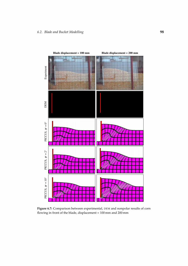
6.2. Blade and Bucket Modelling 98
Blade displacement = 100 mm Blade displacement = 200 mm
Exp
erim
ent
DE
MPI
CC
US,
ψ=
0°PI
CC
US,
ψ=
2°PI
CC
US,
ψ=
10°
Figure 6.7: Comparison between experimental, DEM and nonpolar results of cornflowing in front of the blade, displacement = 100 mm and 200 mm

6.2. Blade and Bucket Modelling 99
Exp
erim
ent
DE
MPI
CC
US,
ψ=
0°PI
CC
US,
ψ=
2°PI
CC
US,
ψ=
10°
Blade displacement = 300 mm Blade displacement = 400 mm
Figure 6.8: Comparison between experimental, DEM and nonpolar results of cornflowing in front of the blade, displacement = 300 mm and 400 mm

6.2. Blade and Bucket Modelling 100
Experiment
Nonpolar = 10°
Nonpolar = 0°
Nonpolar = 2°
Displacement = 100 mm Displacement = 200 mm
Displacement = 300 mm Displacement = 400 mm
Figure 6.9: Comparison of the free surfaces using different dilatancy angles
Curves were fitted to the free surfaces to make a quantitative compari-son of the flow of material (figure 6.9). The free surfaces exhibit the effect ofthe dilatancy angle: with an increase in dilatancy angle, there is an increasein material volumetric expansion. The free surface is the most accuratelypredicted using a dilatancy angle ψ = 2. The value ψ = 2 is assumed forall other simulations.
The simulation was repeated with a Cosserat continuum. The materialproperties used are summarised in table 6.2. The standard set of coefficientsa1, a2 and a3 was used. The moment of inertia J33 was assumed to be thatfor a cylinder with a diameter equal to the characteristic length l which hasbeen taken to be the same order of magnitude as the size of the corn grains.The friction- and dilatancy parameters are calculated as proposed by Tejch-man (1997). For a detailed description of the Cosserat constitutive modelsee Appendix I.5. A comparison of the polar and nonpolar continuum flowpatterns is given in figure 6.10. At a displacement of 100 mm there is goodagreement, but as the blade moves further, the polar continuum seems toshow less dilation than the nonpolar continuum. The curves fitted to thefree surfaces are shown in figure 6.11. From these curves it can be seenthat the nonpolar continuum predicts the free surface the most accurately.The DEM predicted free surface is in close agreement with the polar conti-nuum predicted free surface up to a displacement of 200 mm, but both failto predict the experimental free surface accurately.
The forces that should be applied to the blade to move it at constantvelocity are shown in figure 6.12 for different values of ψ. The force in thevertical x2-direction is negative, which indicates that the material tends to
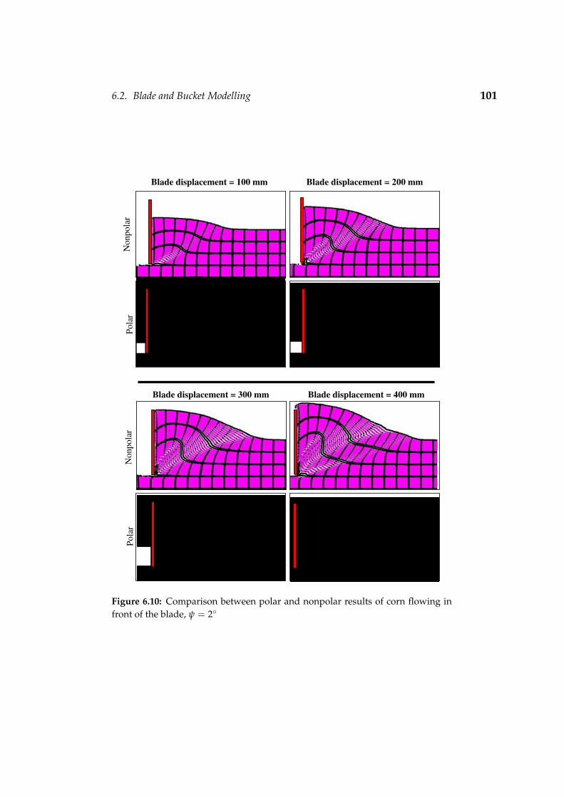
6.2. Blade and Bucket Modelling 101
Blade displacement = 100 mm Blade displacement = 200 mm
Non
pola
rPo
lar
Blade displacement = 300 mm Blade displacement = 400 mm
Non
pola
rPo
lar
Figure 6.10: Comparison between polar and nonpolar results of corn flowing infront of the blade, ψ = 2

6.2. Blade and Bucket Modelling 102
Table 6.2: Corn material properties - Cosserat continuum
Young’s modulus E 2.76 MPa
Poisson’s ratio ν 0.2
Density ρ 778 kg·m−3
Friction angle φ 26
Friction parameter α = sin φ 0.44
Dilatancy angle ψ 2
Dilatancy parameter β = sin ψ 0.035
Cohesion c 0 Pa
Tension cutoff σt 0 Pa
Friction with steel φs 14
Constitutive coefficients a1; a2; a3 0.375;0.125;1
Cosserat shear modulus Gc = 2G 2.3 MPa
Characteristic length l 10 mm
Moment of inertia J33 = 0.5(0.5 l)2 12.5× 10⁻⁶m2
Experiment
Polar = 2°
DEM
Nonpolar = 2°
Displacement = 100 mm Displacement = 200 mm
Displacement = 300 mm Displacement = 400 mm
Figure 6.11: Comparison of the experimental, polar (ψ = 2), nonpolar (ψ = 2)and DEM free surfaces

6.2. Blade and Bucket Modelling 103
0 5 10 15 20 25 30 35 40-200
-100
0
100
200
300
400
500
Displacement, x1 [mm]
Forc
e [N
]
x1 -forces
x2 -forces
Nonpolar = 2°Nonpolar = 10°Nonpolar = 26°Polar = 2°
Figure 6.12: The effect of the dilatancy angle ψ on the blade forces, h = 350 mm
push the blade upwards, hence a negative force should be applied to theblade to prevent vertical movement. Over the first part of the displace-ment the responses, using a nonpolar continuum, are the same because thematerial is in a total elastic state. In the plastic regions, however, there isan increase in blade forces with an increase in dilatancy angle. This phe-nomenon has also been observed for cone penetration tests (Vermeer andDe Borst, 1984). The polar result, with ψ = 2 is also shown. The polar con-tinuum, however, predicts forces 13% lower than the nonpolar continuumwith ψ = 2. The polar continuum also shows an initial elastic stiffnessthat slightly differs from that of the nonpolar continuum. According to Te-jchman (1997), the constitutive constants, a1, a2, a3 and the Cosserat shearmodulus Gc have an influence on the material stiffness.
Using the dilatancy angle ψ = 2 and a nonpolar continuum, the effectof blade depth h on the blade forces is shown in figure 6.13, using depthsh = 150 mm, 250 mm and 350 mm. As expected, the forces increase with anincrease in blade depth. In order to compare the PICCUS results to that fromDEM, experiments and Sokolovski’s method of characteristics (Sokolovski,1954), the average draft forces are calculated. The draft force is defined asthe force needed to push or pull a blade through the material, in the di-
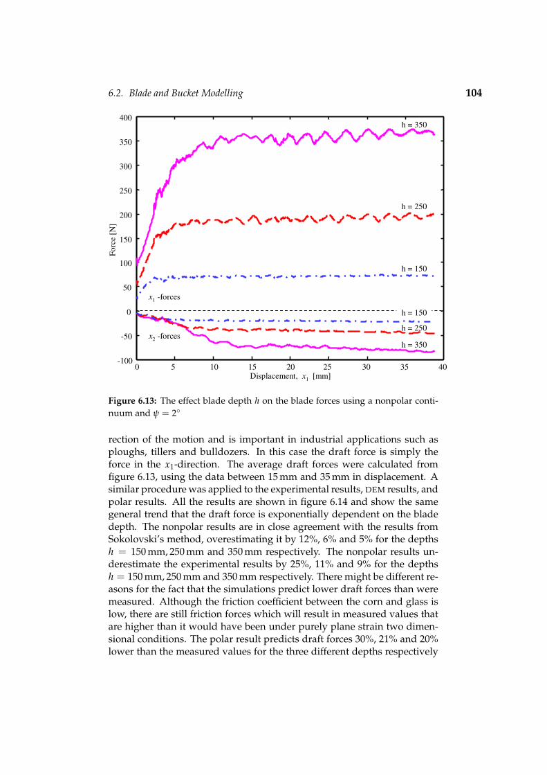
6.2. Blade and Bucket Modelling 104
0 5 10 15 20 25 30 35 40-100
-50
0
50
100
150
200
250
300
350
400
Displacement, x1 [mm]
Forc
e [N
]
h = 350
h = 250
h = 150
h = 350
h = 250
x1 -forces
x2 -forces
h = 150
Figure 6.13: The effect blade depth h on the blade forces using a nonpolar conti-nuum and ψ = 2
rection of the motion and is important in industrial applications such asploughs, tillers and bulldozers. In this case the draft force is simply theforce in the x1-direction. The average draft forces were calculated fromfigure 6.13, using the data between 15 mm and 35 mm in displacement. Asimilar procedure was applied to the experimental results, DEM results, andpolar results. All the results are shown in figure 6.14 and show the samegeneral trend that the draft force is exponentially dependent on the bladedepth. The nonpolar results are in close agreement with the results fromSokolovski’s method, overestimating it by 12%, 6% and 5% for the depthsh = 150 mm, 250 mm and 350 mm respectively. The nonpolar results un-derestimate the experimental results by 25%, 11% and 9% for the depthsh = 150 mm, 250 mm and 350 mm respectively. There might be different re-asons for the fact that the simulations predict lower draft forces than weremeasured. Although the friction coefficient between the corn and glass islow, there are still friction forces which will result in measured values thatare higher than it would have been under purely plane strain two dimen-sional conditions. The polar result predicts draft forces 30%, 21% and 20%lower than the measured values for the three different depths respectively

6.2. Blade and Bucket Modelling 105
0 50 100 150 200 250 300 350 4000
50
100
150
200
250
300
350
400
450
Depth, h [mm]
Ave
rage
dra
ft fo
rce
[N]
Nonpolar
DEM ExperimentSokolovski
Polar
Figure 6.14: Comparison between average draft fores: PICCUS, DEM, experimentsand Sokolovski’s method
and 28%, 14% and %10 lower than the nonpolar results. Tejchman (1997)reports a 30% difference in polar and nonpolar continuum results in mo-delling a strip footing. The percentage difference in polar and nonpolar re-sults compared to experiments seems to decrease with an increase in bladedepth, i.e. an increase in stress. The same phenomenon can be seen by com-paring the polar results to the nonpolar results. The DEM result (Coetzee,2000), compared to the measured values, predicts a higher draft force withh = 150 mm and h = 250 mm and a lower draft force with h = 350 mm
When the blade pushes the material forward, a shear band develops,reaching from the bottom tip of the blade to the free surface. The abilityof PICCUS and DEM to predict these shear bands was investigated. UsingDEM, it can be very difficult to predict the shear bands, but there is defini-tely evidence that such lines exist. Coetzee (2000) made use of the particledisplacement ratio (PDR) to find shear bands. PDR is defined as the ratio ofthe magnitude of the particle displacement vector to the magnitude of theblade displacement vector. The top of figure 6.15 shows the results usingPDR = 0.15, i.e., all the darker particles have been displaced a distance ofat least 0.15 times the displacement of the blade. The experimentally ob-

6.2. Blade and Bucket Modelling 106
Nonpolar
DEM
Experiment Sokolovski
Polar
Figure 6.15: Predicted shear bands using a particle displacement ratio PDR = 0.15,x1 = 15 mm

6.2. Blade and Bucket Modelling 107
served shear band and the line predicted by Sokolovski’s method are alsoshown. The line shown on the figure indicates the centre of the observedshear band. With PDR = 0.15, the predicted shear band falls between theobserved line and the Sokolovski line at the free surface. Closer to the bot-tom edge of the blade, however, the shear band is outside of that predictedby Sokolovski’s method. This is because the particles have a finite sizewhereas in Sokolovski’s method, the shear band is assumed to start at thebottom edge of the blade.
The lower two images in figure 6.15 show similar results from the non-polar and polar continuums respectively. All the material points within thedarker region have PDR ≥ 0.15. The nonpolar continuum predicted shearband meets the free surface at almost exactly the same place as the DEM pre-dicted shear band. Closer to the blade tip, however, the shear band moreclosely follows that of the observed and Sokolovski lines. Contrary to theDEM modelling, using a continuum, there are no particles with a finite size,which causes the DEM shear band to be outside the Sokolovski line. Thepolar continuum predicts a shear band at almost 45 and it is less curvedthan the observed and nonpolar shear band.
The predicted shear band can be manipulated by changing the PDR va-lue to obtain a better fit. A more precise method of predicting the shearband is possible with a continuum method, but not with DEM. Using thenonpolar continuum, figure 6.16 shows all the regions which have a stressstate on the yield surface as lighter (yellow) patches and those which havestress states below the yield surface (elastic state) as darker (red) patches.Two mesh sizes were used, 120 × 70 and 80 × 50. Yields points are con-centrated around the observed and Sokolovski shear bands. The coarsermesh shows more yield points and a broader shear region. Figure 6.17shows the nonpolar shear strain intensity. The shear strain shows a defi-nite band, bounding the observed and Sokolovski shear bands. Again thecoarser mesh predicts a slightly broader shear band than the fine mesh, butthe general shape remains the same.
It is well-known that the Cosserat rotation is an indication of shearbands (Tejchman, 1997). Figure 6.18 shows the rotation for two differentmesh sizes with the rotation at the blade interface unconstrained (free).Again, the shear regions differ from the nonpolar and experimental results,but do agree with the polar displacement field as depicted in figure 6.15.There is little difference in the results from the two different mesh sizes.Figure 6.19 shows the nonpolar shear strain and the polar rotation using a80× 50 mesh rotated through 35 anticlockwise. Comparing the nonpolarresult to that of figure 6.17, shows that the direction of the shear band isonly slightly influenced by the mesh orientation. Comparing the polar re-sult to that of figure 6.18, shows that the shear band is not influenced bythe mesh orientation.
The observed slip line had a width of about 7 - 8 particle diameters, i.e.,

6.2. Blade and Bucket Modelling 108
Experiment Sokolovski
120 X 70
80 X 50
Figure 6.16: Nonpolar yield points: mesh sizes 120× 70 and 80× 50, x1 = 15 mm
70 mm - 80 mm (Coetzee, 2000). The simulations, polar and nonpolar, pre-dict shear bands 60 mm - 80 mm wide. Tejchman (1997) states that if thesize of the elements is smaller than five times the mean grain diameter d50,i.e. 50 mm, the polar results are independent on the mesh size. The 120× 70and 80× 50 had element sizes 10 mm× 10 mm and 15 mm× 14 mm respec-tively. These sizes are well below five times the mean grain diameter.
Figure 6.20 shows the material translational velocity fields in front ofthe blade. Comparing this figure to figure 6.15, it can be seen that thedisplacement field and velocity field, resulting from the polar- and non-polar continuum, is in close agreement. Although the DEM displacementfield is similar to the nonpolar displacement field, there is big differencein the velocity fields. The displacement fields have been calculated aftera 10 mm blade displacement, i.e., it can be viewed as an average velocityfield. The velocity fields, however, are just a snapshot at a specific momentin time. This indicates that using DEM, the particles move in a step-like fa-shion (stick-slip) and it should be averaged over a period of time to get the

6.2. Blade and Bucket Modelling 109
Experiment Sokolovski
120 X 70
80 X 50
Figure 6.17: Nonpolar shear strains for mesh sizes 120 × 70 and 80 × 50,x1 = 15 mm
total effect. The polar continuum velocity field compares well to the DEM
velocity field, but not to the nonpolar velocity field.The standard set of Cosserat coefficients a1, a2 and a3 has been used.
Muhlhaus & Vardoulakis (1987) derived the values of these coefficients bytaking into account slip and rotation in a random assembly of circular rods.Tejchman (1997) investigated the effect of the Cosserat material parameterson biaxial simulations and concludes that the standard set of parametersturned out to be useful and sufficient in numerical calculations involvinglocalisation. The influence of a3 on the results was rather insignificant and,in general, the larger the difference between a1 and a2, the larger the non-symmetry of the stress tensor. Tejchman (1997) also showed that when thefollowing set is used, a1 = 0.25, a2 = 0.25, a3 = 0.5, the response is slightlyless stiff compared to the standard set. It was found that by changing thevalue of Gc from Gc = 2G to Gc = 0.5G the draft force on the blade decre-

6.2. Blade and Bucket Modelling 110
120 X 70
80 X 50
Figure 6.18: Polar rotations [rad] for mesh sizes 120× 70 and 80× 50, x1 = 15 mm
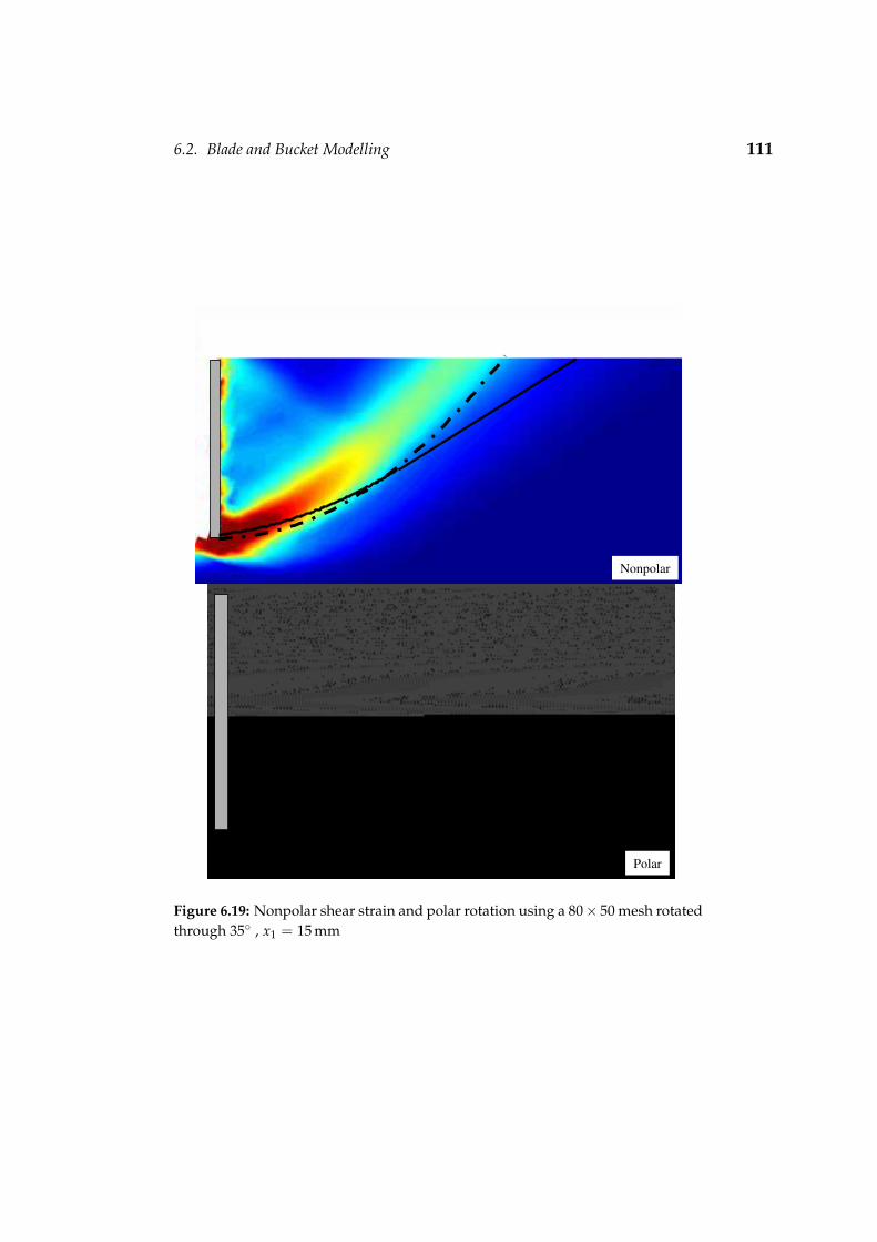
6.2. Blade and Bucket Modelling 111
Polar
Nonpolar
Figure 6.19: Nonpolar shear strain and polar rotation using a 80× 50 mesh rotatedthrough 35 , x1 = 15 mm

6.2. Blade and Bucket Modelling 112
DEM
Sokolovski
Nonpolar
Experiment
Polar
Simulation
Simulation
Figure 6.20: The velocity fields in front of the blade, x1 = 15 mm
ased by 1.3%. Changing the internal length from l = 10 mm to l = 2 mm,the draft force decreased by only 1.9%. These results show that the modelis not sensitive to changes in the values of Gc and l.
Figure 6.21 shows the normal and shear stress at the blade as predic-ted by the nonpolar continuum and Sokolovski’s method. The continuumresults were obtained from the nodal forces acting on the blade. The ir-regularity in the stress close to the bottom edge of the blade is due to the

6.2. Blade and Bucket Modelling 113
unit normal vector at the bottom node which is not horizontal and possiblestress concentrations. The nonpolar results are in good agreement with theSokolovski predictions. Figure 6.22 shows the polar continuum results fortwo boundary conditions: no rotation at the blade wc = 0 and free rotationat the blade. The polar results predict normal and shear stresses lower thanthat of the nonpolar continuum and Sokolovski’s method. Having no rota-tion or free rotation at the blade has little effect on the normal stress, but theshear stress with free rotation, is almost half the stress when no rotation isallowed. This means that the rotation has an influence on the friction bet-ween the material and the blade. This has also been observed by Tejchman(1997).
Figure 6.23 shows the DEM contact force chains between particles andbetween the particle and the blade. The thickness of the force chains is di-rectly proportional to the magnitude of the contact force. In this particularcase there were 50 contacts between particles and the blade. Taking theaverage contacting force of two neighbouring contacts and dividing it bythe distance between the contacting points along the blade, the stress at theblade could be estimated. Due to the particles moving in a step-like fashion,a time average was used to calculate the stress at the blade. The averagewas calculated between a blade displacement of 18 mm and 22 mm and theresult is shown in figure 6.24. The normal and shear stress are lower thanthe stresses predicted by Sokolovski’s method.

6.2. Blade and Bucket Modelling 114
0 1 2 3 4 5 6 7 8 9 100
50
100
150
200
250
300
350
400
Stress [kPa]
Dis
tanc
e al
ong
blad
e [m
m]
Normal stress, Sokolovski
Shear stress, Sokolovski
Normal stress, Nonpolar
Shear stress, Nonpolar
Figure 6.21: Normal and shear stress at the blade for h = 350 mm: Nonpolarcontinuum and Sokolovski’s method, x1 = 20 mm

6.2. Blade and Bucket Modelling 115
0 1 2 3 4 5 6 7 8 9 100
50
100
150
200
250
300
350
400
Stress [kPa]
Dis
tanc
e al
ong
blad
e [m
m]
Normal stress, Sokolovski
Shear stress, Sokolovski
Normal stress, Rotation
Shear stress, Rotation
Shear stress, No rotation
Normal stress, No rotation
Figure 6.22: Normal and shear stress at the blade for h = 350 mm: Polarcontinuum, with and without rotation at the blade, and Sokolovski’s method,x1 = 20 mm
Figure 6.23: Force chains at the blade for h = 350 mm, x1 = 20 mm

6.2. Blade and Bucket Modelling 116
0 2 4 6 8 10 12 140
50
100
150
200
250
300
350
400
Pressure [kPa]
Dis
tanc
e al
ong
blad
e [m
m]
Normal pressure, Sokolovski
Shear pressure, Sokolovski
Normal pressure, DEM
Shear pressure, DEM
Figure 6.24: Normal and shear pressures at the blade for h = 350 mm: DEM andSokolovski’s method

6.2. Blade and Bucket Modelling 117
6.2.6 Bucket Modelling
Coetzee (2000) investigated the ability of DEM to simulate the filling of ascaled model bucket with corn grains. The bucket used in experiments wasa dragline type of bucket with freedom of motion in the vertical direction.The vertical motion of the bucket was determined by the bucket weight andthe effect of the material flowing into the bucket. The bucket was given aconstant velocity of 10 mm·s−1 in the x1-direction and the drag force andvertical displacement recorded. The vertical velocity was found to be con-stant and used as input to the DEM models and in this evaluation of PICCUS.The 2.0 m× 0.7 m domain was divided into 200× 100 elements, each of size10 mm× 7 mm. The bottom boundary was fixed in the horizontal, verticaland rotational (polar) directions and the two side boundaries in the hori-zontal and rotational (polar) directions. The boundaries were too far awayfrom the bucket to have a significant effect on the results. No polar rotationwas allowed at the bucket-material interface. The material stresses wereinitialised using a coefficient of earth pressure Ko = 1− sinφ. The bucketwas created with its bottom surface against the material free surface withthe tooth already engaged into the material.
Figure 6.25 shows the measured, nonpolar continuum, polar continuumand DEM draft force on the bucket. The nonpolar draft force correspondswell to the measured force up to a displacement of 600 mm, but thereafter itunder predicts the force and at 800 mm the error is 12%. The DEM predictedforce is more-or-less 20 N lower than the measured force up to a displace-ment of 600 mm. The polar continuum predicts a draft force lower than themeasured force and the nonpolar predicted force.
Figure 6.26 to figure 6.29 show the experimental, DEM, nonpolar con-tinuum and polar continuum filling process at increments of 100 mm inbucket displacement. Figure 6.30 shows the curves fitted to the materialfree surface during the filling process. During the initial stages of filling,there is an upheave of material right above the tooth. Up to a displa-cement of 200 mm the nonpolar continuum predicts the free surface andthe upheave the most accurately while the polar continuum predicts lessupheave of material during these initial stages of filling. Between the dis-placements of 300 mm and 600 mm, the polar continuum predicts the freesurface more accurately than the nonpolar continuum. Compared to theexperimental free surface, the DEM model predicts less upheave of materialduring the entire filling process.

6.2. Blade and Bucket Modelling 118
100 200 300 400 500 600 700 8000
50
100
150
200
250
x1-Displacement [mm]
Dra
ft fo
rce
[N
]
Experiment
Nonpolar
DEMPolar
Figure 6.25: Bucket draft force as measured and predicted by the nonpolar conti-nuum, polar continuum and DEM

6.2. Blade and Bucket Modelling 119
Displacement = 100 mm Displacement = 200 mmE
xper
imen
tD
EM
Non
pola
rPo
lar
Figure 6.26: The flow of corn into the bucket: displacement = 100 mm - 200 mm
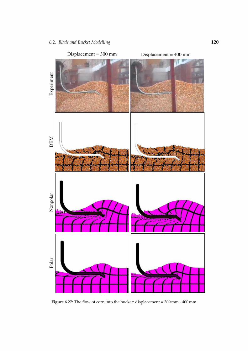
6.2. Blade and Bucket Modelling 120
Displacement = 300 mm Displacement = 400 mmE
xper
imen
tD
EM
Non
pola
rPo
lar
Figure 6.27: The flow of corn into the bucket: displacement = 300 mm - 400 mm

6.2. Blade and Bucket Modelling 121
Displacement = 500 mm Displacement = 600 mmE
xper
imen
tD
EM
Non
pola
rPo
lar
Figure 6.28: The flow of corn into the bucket: displacement = 500 mm - 600 mm

6.2. Blade and Bucket Modelling 122
Displacement = 700 mm Displacement = 800 mmE
xper
imen
tD
EM
Non
pola
rPo
lar
Figure 6.29: The flow of corn into the bucket: displacement = 700 mm - 800 mm

6.2. Blade and Bucket Modelling 123
Experiment
Polar = 2°
DEM
Nonpolar = 2°
100 mm 200 mm
300 mm 400 mm
500 mm 600 mm
700 mm 800 mm
Figure 6.30: Comparison of the free surface of the material flowing into the bucket

6.2. Blade and Bucket Modelling 124
Rowlands (1991) made use of mixtures of millet, peas and corn in histest rig which is similar to the rig used by Coetzee (2000). The observationof the filling behaviour led to the development of a theory that describes theflow characteristics and patterns of material entering the bucket. Rowlands(1991) named this concept the Shear Zone Theory. He observed that definiteplanes of shear formed between distinct moving material regimes. Theseshear planes changed orientation and location depending on initial setupand during the filling process itself.
The experiments by Coetzee (2000) with corn confirmed this theory. Thegeneralised theory is shown in figure 6.31. The movements of the materialrelative to the bucket are indicated by the arrows. The Virgin Material re-mains largely undisturbed until the final third of the drag during which"bulldozing" occurs. The Initial Laminar Layer flows into the bucket duringthe first third of the drag. After entering to a certain distance, this layerfails at the bucket lip and subsequently becomes stationary with respect tothe bucket for the remainder of the drag. With the laminar layer becomingstationary, a new zone, the Active Flow Zone, develops. In this zone, the ma-terial displacement is predominantly in the vertical direction. The ActiveDig Zone is located above the teeth and bucket lip. This area develops asmaterial starts to enter the bucket and increases in size after failure of theInitial Laminar Layer. In this zone, the Virgin Material fails and either flowsinto the bucket as part of the laminar layer during the first part of filling ormoves into the Active Flow Zone during the latter part of filling. The DeadLoad that has resulted from "live" material in the Active Flow Zone ramps upand over the Initial Laminar Layer. Some of the material in the Initial LaminarLayer fails and starts to form part of the Dead Load.
During the experiments two shear bands could be observed. The oneextended from the tip of the tooth up to the free surface. This is knownas the Cutting Shear Band. The second line is the one between the InitialLaminar Layer and the Dead Load, called the Dead Load Shear Band. The DeadLoad Shear Band stretches from the tooth up to the free surface with an angleclose to the material internal friction angle (measured relative to the bottompart of the bucket). This is indicated by the dotted line in figure 6.31.
To investigate the ability of DEM to predict the shear zone theory, Coet-zee (2000) made use of the particle displacement ratio PDR. The bucket wasmoved through the material and "paused" after each 100 mm. The displace-ment vector of each particle was then set to be zero after which the bucketwas given a further displacement of 10 mm - 15 mm. The particles werethen coloured according to their PDR values which is defined as the ratioof the magnitude of the particle displacement vector to the bucket displa-cement vector. The same procedure has been used with the PICCUS resultsand are shown in figure 6.32 to figure 6.34 for displacements of 100 mm,500 mm and 800 mm. All three methods (DEM, polar and nonpolar PICCUS)are capable of predicting the different flow zones, although the orientation

6.2. Blade and Bucket Modelling 125
Active Dig ZoneInitial Laminar Layer
Active Dig Zone
Initial Laminar Layer
Active Flow Zone
Virgin Material
Active Dig Zone
Dead Load
Active Flow Zone
Initial Laminar Layer
(a)
(c)
(b)
Shear Band
Shear Band
Shear BandDead Load Shear Band
Virgin Material
Virgin Material
Figure 6.31: The Shear Zone Theory developed by Rowlands (1991)

6.2. Blade and Bucket Modelling 126
of the shear bands between the zones differ slightly.The prevention of excessive wear on buckets plays a very important
role in bucket design. Special replaceable wear packages are designed andadded to buckets. In order to minimise and predict bucket wear, the con-tact forces or pressures at the bucket-material interface should be known.From a DEM model all the particle-bucket contacts are known. The con-tact position, normal and tangential forces and the particle velocity areavailable at each contact and can be used to predict bucket wear. Thirtyto forty years ago Finnie (1960, 1972) developed a simple model for pre-dicting wear. The model essentially uses the kinetic energy of the inco-ming particle and knowledge about the impact angle to predict wear rates.Cleary (1998b) modelled bucket filling with DEM and made use of the Fin-nie model to predict the wear. Realistic wear patterns were obtained, butno experimental data was available for comparisons of the flow patterns,drag forces, wear patterns and wear rates.
Figure 6.35 and figure 6.36 show the normal and shear stress on theinside of the bucket. For the DEM models the contact normal and shearforces were used to calculate the stress, while for the PICCUS models thenodal forces were used. The maximum stresses occur on the tooth. TheDEM predicted stresses are in general lower than the nonpolar predictedpressures and the polar predicted pressures lower than both the nonpolarand DEM predicted stress.
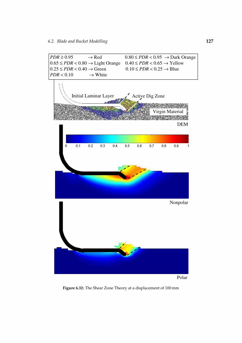
6.2. Blade and Bucket Modelling 127
Nonpolar
Initial Laminar Layer Active Dig Zone
Virgin Material
DEM
PDR ≥ 0.95 → Red 0.80 ≤ PDR < 0.95 → Dark Orange0.65 ≤ PDR < 0.80 → Light Orange 0.40 ≤ PDR < 0.65 → Yellow0.25 ≤ PDR < 0.40 → Green 0.10 ≤ PDR < 0.25 → BluePDR < 0.10 → White
Polar
Figure 6.32: The Shear Zone Theory at a displacement of 100 mm
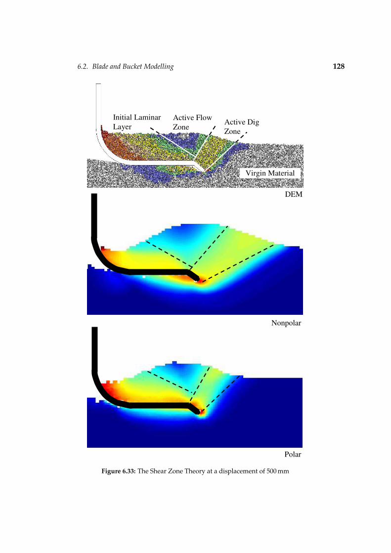
6.2. Blade and Bucket Modelling 128
Virgin Material
Active Dig Zone
Initial LaminarLayer
Active Flow Zone
DEM
Nonpolar
Polar
Figure 6.33: The Shear Zone Theory at a displacement of 500 mm

6.2. Blade and Bucket Modelling 129
Virgin Material
Dead Load
DEM
Nonpolar
Polar
Figure 6.34: The Shear Zone Theory at a displacement of 800 mm

6.2. Blade and Bucket Modelling 130
Nonpolar:
max = 15.1 kPa
DEM:
max = 12.8 kPa
Polar:
max = 9.8 kPa
Figure 6.35: The normal stress on the inside of the bucket at a displacement of800 mm
Nonpolar:
max = 3.5 kPa
DEM:
max = 3.2 kPa
Polar:
max = 2.3 kPa
Figure 6.36: The shear stress on the inside of the bucket at a displacement of800 mm

6.3. Silo Modelling 131
6.3 Silo Modelling
Roughly one-half of the products and about three-quarters of the raw ma-terials of the chemical industry are in the form of granular material that areusually stored in silos or bunkers (Yang and Hsiau, 2001). Although thesilo is widely used, definite theories for the flow of material in silos are notavailable (Yang and Hsiau, 2001).
Yang & Hsiau (2001) investigated silo discharge using experiments andDEM simulations. They, however, used a "perfect" material: a single columnof equally sized glass beads. It is relatively easy to determine the particlemicro parameters such as particle-particle friction and contact stiffness forsuch a material. The modelling of irregular shaped particles, such as sandor seed grains, is not addressed. They, however, obtained good results bycomparing flow rates and flow patterns. Masson & Martinez (2000) usedequally sized acrylic cylinders in experiments and compared the results toDEM simulations. Friction and contact stiffness proved to play a major rolein the flow and the stress field during filling and discharging.
Rectangular planform silos have not been studied as often as circularsilos, and relatively little detailed information exists on pressure patternswhich develop on their walls (Brown et al., 2000). Rectangular silos haveadvantages over circular silos when available space is limited and simpli-city in construction is important. Brown et al. (2000) investigated the pres-sure on a model rectangular silo using a series of strain gauges and wallpressure sensors. Loading of the silo was achieved by filling a small hop-per suspended above the silo. The hopper was then discharged into the silothrough its base. Brown et al. (2000) state that it is known that filling a siloin such a matter can display anisotropy, but focused on repeatability ratherthan uniformity. After filling, the wall pressures also displayed asymmetry,which could only be attributed to the filling process.
Martinez et al. (2002) investigated silo discharge using FEM with remes-hing. The authors conclude that the remeshing introduces additional costsand meshless methods can avoid this inconvenience. Karlsson et al. (1998)used FEM based on the Eulerian frame of reference. The major disadvan-tage of this approach is that all boundaries are fixed. The upper free surfacein a silo requires refilling to be fixed, and as a result it is not possible to si-mulate the complete discharging process. However, the redistribution ofstresses when the flow develops is very fast, and the upper surface doesnot move much during this time. Thus, the Eulerian approach could beused to simulate only the initial stress transients.
As part of this research, a model silo was build to investigate the flowof material out of a plane strain flat bottomed silo. The focus is mainly onflow patterns and flow rate. The flow pattern in a silo is of great importancewhen handling material that degenerates with time. Then it is importantto achieve the first-in-first-out storage principle (Karlsson et al., 1998). The

6.3. Silo Modelling 132
0 10 20 30 40 50 60 70 80 900
5
10
15
20
25
30
35
40
45
50
55
Normal pressure [kPa]
Shea
r pr
essu
re [
kPa]
Figure 6.37: The sand shear test results
model silo used for the experiments had dimensions of 310 mm wide, amaximum fill height of 600 mm and a depth of 730 mm. All the sides wereconstructed of glass and the opening width could be varied. The door couldbe opened without affecting the initial flow and the depth to width ratiowas high enough for the flow to be two-dimensional.
Two types of material were used: corn and sand. The corn was fromthe same batch as used by Coetzee (2000), so the macro properties wereknown for continuum modelling and the micro properties for DEM model-ling. A dry graded silica sand was used with the following main consti-tuents: SiO2 = 98% and Fe2O3 = 0.18%. A shear test (figure 6.37) and anoedometer test were used to determine the sand friction angle and elasticmodulus respectively. The bottom half of the shear box was replaced by aglass panel to measure the friction between the sand and glass. Table 6.3summarises the measured sand properties and the different values usedin the material models. The Drucker-Prager constitutive model was usedfor modelling both the corn and the sand. The same commercial package(PFC2D) used by Coetzee (2000) was used for the DEM simulations.
The sand grains had an average size of more or less 1 mm and fromthere the internal length l = 1 mm. Again the moment of inertia has been

6.3. Silo Modelling 133
Table 6.3: Sand material properties
Young’s modulus E 21.5 MPa
Poisson’s ratio ν 0.2
Density ρ 1286 kg·m−3
Friction angle φ 32
Cosserat friction parameter α = sin φ 0.53
Drucker-Prager friction parameter qφ 0.52
Dilatancy angle ψ 2, 5
Cosserat dilatancy parameter β = sin ψ 0.035, 0.174
Drucker-Prager dilatancy parameter β 0.040, 0.098
Cohesion c 0.9 kPa
Tension cutoff σt 0 Pa
Friction with glass φs 18
Constitutive coefficients a1; a2; a3 0.375;0.125;1
Cosserat shear modulus Gc = 2G 17.9 MPa
Characteristic length l 1 mm
Moment of inertia J33 = 0.5(0.5 l)2 12.5× 10⁻⁸m2
calculated by assuming a cylinder with a diameter equal to the internallength. The Drucker-Prager dilatancy and friction parameters were calcu-lated using equation H.6.2. It is difficult to measure the bulk density in aflowing granular material and the assumption of constant density is madefor the sake of simplicity and numerical efficiency. The silo was filled inthe same way used by Brown et al. (2000). A hopper was suspended abovethe silo and its door (200 mm× 200 mm) opened until the silo was filled.The top surface was then carefully levelled. In the DEM model, the sameprocedure was used and in the PICCUS models the material was createdlayer-by-layer and allowed to reach an equilibrium state after each layerwas added. Coloured grains were used to create layers within the ma-terial which are used to compare flow patterns. In the PICCUS models asymmetry plane was used and friction applied at the walls. No polar ro-tations were allowed at the walls which is the case for relatively smoothwalls (Tejchman, 1997). The 40× 50 rectangular mesh had elements of size3.875 mm× 10 mm. Time steps of ∆t = 5× 10⁻⁵s and ∆t = 2× 10⁻⁵s wereused for the modelling of corn and sand respectively. In the DEM models no

6.3. Silo Modelling 134
symmetry plane was used and as a result the flow patterns are not perfectlysymmetric.
Figure 6.38 and figure 6.39 show the flow of corn out of the silo with theopening w = 45 mm and the initial fill height h = 500 mm. The experimen-tal, polar, nonpolar and DEM results are shown at increments of one second,up to eight seconds. Looking at the DEM results, there is good agreementwith the experimental results with regard to flow patterns although theDEM discharge rate is higher. Qualitatively, the nonpolar flow patterns andflow rate compare well to the experiment. The polar continuum shows ahigher flow rate and there is a definite difference in the flow patterns com-pared to the nonpolar continuum. To make a quantitative comparison ofthe flow patterns is difficult. The flow rate can, however, be comparedquantitatively. The mass of the material within the silo was measured byhanging the silo from a load cell. The question however arises whether themeasured mass of the material during discharge is a true representation ofthe flow rate. Close to the silo opening the free falling material will not con-tribute to the measured value although the material is still within the silo.The acceleration and deceleration of the material as it flows in the silo willalso create dynamic effects. The flow rate is defined as the rate at whichmaterial flows through the silo opening measured in kg·s−1. The results ofthe DEM simulations were used to clarify this point. Figure 6.40 shows thetwo methods of calculating the mass of material within the silo. The firstmethod is to simply add up the mass of all the particles above the silo ope-ning at each time step. The second method is to add the resultant verticalforce of all the walls at each time step. The second approach is similar tothe experiments. From the figure it can be seen that the resultant verticalforce on the silo walls show high fluctuations due to the collisions betweenthe particles and the walls. The result from the first method is a very goodfit to the result from the second method and it can be concluded that themeasured values are a good representation of the material mass in the silo.
Figure 6.41 shows the corn mass within the silo as a function of timefor two openings: w = 45 mm and w = 80 mm. For both openings, DEM
predicts a higher flow rate than the measured rates. With w = 45 mm,the nonpolar continuum predicts a higher flow rate and with w = 80 mma lower flow rate. The polar continuum predicts a higher flow rate forboth openings and the results are in close agreement with the DEM results.Figure 6.42 shows the sand mass within the silo as a function of time withw = 45 mm and the initial fill height h = 550 mm. Since the dilatancy anglecould not be measured, two values ψ = 2 and 5 were used. As expected,with an increase in dilatancy angle there is a decrease in mass flow fromthe silo. The results with ψ = 2 are closer to the measured values and asin the case with corn, the polar continuum predicts a higher flow rate thanthe nonpolar continuum. The dilatancy angle for loose sand is only a fewdegrees according to (Vermeer and De Borst, 1984).

6.3. Silo Modelling 135
Experiment Nonpolar Polar DEMt = 1 s
t = 2 s
t = 3 s
t = 4 s
Figure 6.38: Corn flowing from a silo with w = 45 mm

6.3. Silo Modelling 136
Experiment Nonpolar Polar DEM
t = 5 s
t = 6 s
t = 7 s
t = 8 s
Figure 6.39: Corn flowing from a silo with w = 45 mm continues

6.3. Silo Modelling 137
0 2 4 6 8 10 120
20
40
60
80
100
120
Time [s]
Mas
s / F
orce
[k
g]
Vertical force on all the walls
Sum of all particles’ mass
Figure 6.40: The two methods of calculating the mass flow out of the silo withDEM, w = 45 mm
DEM simulations of sand were not performed since it would be imprac-tical to model each individual particle. The computing power needed tomodel such a large number of particles was not available. If, however, itcould be computed, a series of DEM numerical experiments first needs tobe performed to determine the particle micro properties suitable for mo-delling the sand.

6.3. Silo Modelling 138
0 1 2 3 4 5 6 7 8 9 10 11 12 13 14 150
10
20
30
40
50
60
70
80
90
100
Time [s]
Mas
s in
silo
[kg
]
w = 80 mm w = 45 mm
Experiment
NonpolarDEMPolar
Figure 6.41: The flow rate of corn out of the silo
0 1 2 3 4 5 6 7 8 9 10 110
20
40
60
80
100
120
140
160
180
Time [s]
Mas
s in
silo
[kg
]
Experiment
Nonpolar, = 2°Nonpolar, = 5°Polar, = 2°
Polar, = 5°
Figure 6.42: The flow rate of sand out of the silo with w = 45 mm

6.4. Computing Times 139
6.4 Computing Times
DEM, nonpolar continuum and polar continuum simulations were used tomodel corn flowing from the silo. The run time to model the first 10 s of silodischarge is shown in table 6.4 for each simulation. The simulations wereall run on a Pentium IV 2.4 GHz with 512 MB RAM. The DEM model had5348 circular particles making up 2674 clumps. Four PICCUS models wereused: a polar continuum with a symmetry plane and the full geometry, anonpolar continuum with a symmetry plane and the full geometry. Thefull geometry (310 mm × 500 mm) was divided into 80 × 50 = 4000 ele-ments and the geometry with the symmetry plane (155 mm× 500 mm) wasdivided into 40× 50 elements. A time step of ∆t = 5× 10⁻⁵ was used in allthe simulations including DEM. In table 6.5, a comparison of the run timesis made. When a symmetry plane is used, the nonpolar and polar conti-nuum methods are both quicker than the DEM simulation by 39% and 9.3%respectively. When the full geometry is modelled, the number of degrees-of-freedom is more or less doubled and the simulations slower by 134%and 266.5% compared to the DEM simulation respectively. The polar conti-nuum is slower than the nonpolar continuum by more or less 50% whichis expected because of the three degrees-of-freedom compared to the twodegrees-of-freedom per node of the nonpolar continuum. In the DEM mo-dels, the physical size of the corn grains was used to model the particles.This lead to run times which are comparable to PICCUS run times. To mo-del materials with relatively small particles such as sand, it would requirea large number of particles, and more computing power if physical particlesizes are used. On the other hand, the continuum method with the samemesh size should still yield good results.
Table 6.4: Run time to model 10 s of silo discharge
Model Run time Number of particles Initial DOF
DEM 2.92 h 5348 –
Nonpolar symmetry 1.78 h 8000 4011
Nonpolar full 6.83 h 16000 8022
Polar symmetry 2.65 h 8000 6102
Polar full 10.70 h 16000 11983

6.4. Computing Times 140
Table 6.5: Comparison of the run times of the different methods used
DEM Nonpolar Nonpolar Polar Polar
symmetry full symmetry full
DEM –
Nonpolar sym. -39.0% –
Nonpolar full 134.0% 283.7% –
Polar sym. -9.3% 48.9 -61.2% –
Polar full 266.5% 501.1% 56.7% 303.8% –

Chapter 7
Concluding Remarks andRecommendations
A Particle-in-Cell code (PICCUS) was developed to model polar (Cosserat)and nonpolar (classic) continua subjected to large deformations and displa-cements under plane strain conditions. The no-slip contact which is a na-tural consequence of the PIC method has been relaxed by the implementa-tion of a contact algorithm. The algorithm is based on the Coulomb frictiontheory and is applied at the boundary nodes of two bodies in contact. Threenonpolar continuum constitutive models have been implemented: elastic,Drucker-Prager and Mohr-Coulomb models. The Ducker-Prager model re-duces to the von Mises model and the Mohr-Coulomb model to the Trescamodel if the material friction angle is set to zero. Two polar continuumconstitutive models have been implemented: elastic and a Drucker-Pragertype of model. A rigid body model has also been implemented for the mo-delling of anchors, strip footings, blades and buckets. No strain softeningor hardening has been used although it has been implemented as part ofthe nonpolar Mohr-Coulomb model and the polar Drucker-Prager model.
Various simulations were performed to validate the implementation ofthe nonpolar continuum. The simulation of an elastic steel disk impactingon an elasto-plastic aluminium target was compared to published data ofa similar simulation and experimental data. A comparison of the pene-tration depth as a function of time showed good agreement and the finaldepth compared well to experimental values. This demonstrates the abilityof PIC to model large displacements, deformations and the no-slip contactbetween two different bodies.
The simulation of an elastic disk rolling down an elastic inclined surfacewas used to validate the contact model. The centre position of the disk, asa function of time, was compared to analytical results. Different frictioncoefficients, incline angles and mesh sizes were used. The results showthat an accuracy of 0.5% can be achieved, although the analytical modelassumes a rigid disk and surface.
The impact of two elastic bodies was modelled to show the conserva-tion of momentum and energy. The results show that the linear momentumand the total energy are generally conserved although small gains/dissipationscould be observed with an increase in time step size.
The modelling of an oedometer test was used to validate the implemen-tation of the Mohr-Coulomb constitutive model and the ability to modelplastic flow where the stress point evolves along a shear-shear edge of the
141

142
Mohr-Coulomb criterion in the principal stress space.The method of characteristics was proposed by Sokolovski to model the
passive case of a static retaining wall. This theory can also be used to modelthe initial stages of a flat blade pushing against a "wall" of material. Fromthis theory, the normal and shear forces acting on the blade as well as theshear band can be determined. Simulations were performed with a blade atdifferent depths h, and the forces and shear bands were compared to resultsfrom Sokolovski’s method. The results showed that the yield points are agood indicator of the shear band and that the forces acting on the bladeconverge with mesh refinement.
The different problems analysed, indicate that PIC can be used to mo-del applications where the displacements are relatively small (strip foo-tings and anchor pull-out tests) and where large deformations occur (silodischarging). No special contact elements are needed to model frictionalcontacts (blade and bucket modelling).
The analysis of a strip footing on an elastic mass was investigated. As-suming an elastic mass, an analytical solution to this problem is availableand the stresses in the material could be compared to the analytical solu-tion. The results indicated that the stresses in the material can be accuratelypredicted. A more realistic analysis of two strip footing problems was alsodone. In this case, an elasto-plastic material was used to model clay. Abearing capacity and a strip footing close to a vertical cut were analysed.Published data from field tests under plane strain conditions was used forcomparisons. Triaxial tests on the clay were previously performed and thepublished data could be used to determine the clay material properties.The FEM code PLAXIS was also used for comparisons with good results.
Anchors form an important component of civil engineering projects.They are typically used to support structures such as towers, bridges androofs. An anchor pulled in the vertical direction and one pulled at 45 weremodelled. Published experimental data from anchor pull-out tests wereused for comparisons. The results show that the limit load on the anchorscould be accurately predicted to within 5% of the measured values.
Draglines excavators are used to remove blasted overburden from opencast mines to expose the coal deposits beneath for mining. Draglines arean expensive and essential part of mine operations. DEM simulations ofbucket filling have been done in the past, but not bucket filling with a con-tinuum method. The results obtained here shows that bucket filling canbe modelled with both a nonpolar and a polar continuum. The nonpolarcontinuum predicted draft forces more accurately, but the polar continuummodelled the flow patterns of material into the bucket more accurately. Itwas demonstrated that the normal and shear stresses on the bucket can bepredicted. The highest pressures, as expected, acted on the tooth. It shouldbe possible to use these pressures to predict the bucket wear.
The modelling of a flat blade was used to investigate the forces acting
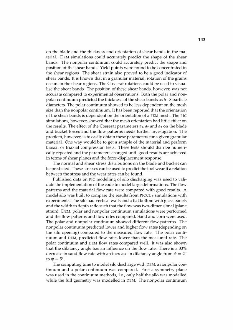
143
on the blade and the thickness and orientation of shear bands in the ma-terial. DEM simulations could accurately predict the shape of the shearbands. The nonpolar continuum could accurately predict the shape andposition of the shear bands. Yield points were found to be concentrated inthe shear regions. The shear strain also proved to be a good indicator ofshear bands. It is known that in a granular material, rotation of the grainsoccurs in the shear regions. The Cosserat rotations could be used to visua-lise the shear bands. The position of these shear bands, however, was notaccurate compared to experimental observations. Both the polar and non-polar continuum predicted the thickness of the shear bands as 6 - 8 particlediameters. The polar continuum showed to be less dependent on the meshsize than the nonpolar continuum. It has been reported that the orientationof the shear bands is dependent on the orientation of a FEM mesh. The PIC
simulations, however, showed that the mesh orientation had little effect onthe results. The effect of the Cosserat parameters a1, a2 and a3 on the bladeand bucket forces and the flow patterns needs further investigation. Theproblem, however, is to easily obtain these parameters for a given granularmaterial. One way would be to get a sample of the material and performbiaxial or triaxial compression tests. These tests should than be numeri-cally repeated and the parameters changed until good results are achievedin terms of shear planes and the force-displacement response.
The normal and shear stress distributions on the blade and bucket canbe predicted. These stresses can be used to predict the tool wear if a relationbetween the stress and the wear rates can be found.
Published data on PIC modelling of silo discharging was used to vali-date the implementation of the code to model large deformations. The flowpatterns and the material flow rate were compared with good results. Amodel silo was built to compare the results from PICCUS simulations withexperiments. The silo had vertical walls and a flat bottom with glass panelsand the width to depth ratio such that the flow was two-dimensional (planestrain). DEM, polar and nonpolar continuum simulations were performedand the flow patterns and flow rates compared. Sand and corn were used.The polar and nonpolar continuum showed different flow patterns. Thenonpolar continuum predicted lower and higher flow rates (depending onthe silo opening) compared to the measured flow rate. The polar conti-nuum and DEM, predicted flow rates lower than the measured rate. Thepolar continuum and DEM flow rates compared well. It was also shownthat the dilatancy angle has an influence on the flow rate. There is a 33%decrease in sand flow rate with an increase in dilatancy angle from ψ = 2
to ψ = 5.The computing time to model silo discharge with DEM, a nonpolar con-
tinuum and a polar continuum was compared. First a symmetry planewas used in the continuum methods, i.e., only half the silo was modelledwhile the full geometry was modelled in DEM. The nonpolar continuum
144
simulations ran 39.0% quicker and the polar continuum simulation 9.3%quicker than the DEM simulation. The full geometry was then also mo-delled with the continuum methods. The number of degrees-of-freedomdoubled and it was found that the nonpolar continuum simulation was 2.3times slower than the DEM simulation and the polar continuum simulation3.7 times. The polar continuum is in general 50% slower than the nonpolarcontinuum. It should, however, be noted that a relatively small numberof particles was used in the DEM model. If a material such as sand wouldbe modelled, a large number of particles is required and computing timeswould be orders higher. DEM also has the disadvantage that numerical ex-periments have to be conducted to determine all the micro properties ofthe material. This is not needed for continuum methods as the materialproperties follows directly from experiments.
Granular flow can only be modelled as a continuum as long as the ma-terial behaves like a continuum. If the material consists of a few big rocks,the behaviour would be more discrete than continuous and better model-led by DEM. There is no clearly defined boundary and more research isneeded to determine when a material can be modelled as a continuum ornot.
Good results were obtained without the use of strain softening or strainhardening. Further research is needed to determine the effect of strain sof-tening and strain hardening on applications such as bucket filling. Lossof ellipticity of the governing equations when nonpolar softening is used,leads to mesh size and mesh alignment dependence. Thus, when strainsoftening is used, a polar continuum should be used to overcome this pro-blem.
No problems are expected in extending the code to model three dimen-sional and axisymmetric problems. The three-dimensional Cosserat conti-nuum has already been used by other researchers to model bone structures.The general feeling is that if a two-dimensional continuum method is ex-tended to three dimensions, the penalty paid in computing times would beless then when a two-dimensional DEM code is extended to three dimensi-ons. This, however, needs to be investigated.
Except for the modelling of the strip footing on clay, mainly cohesion-less materials were analysed. A further extension of this research would beto include material cohesion and adhesion between the blade/bucket andsoil.
It can be concluded that a continuum method can be used to accuratelymodel the filling of an excavator/dragline bucket. This technology can nowbe applied to industrial applications: Buckets can be optimised in terms offill rates (time needed to fill a bucket), energy consumption and wear.

Appendix A
Notation and Basic Principles
A.1 Introduction
Matrix tensor (vector) notation and index notation are described. Matrixtensor notation proposed by Hassenpflug (1993) is used. All vectors are in3-dimensional Euclidean space (R3). The description of the notation usedis important for understanding and following the mathematical derivationsand formulations in the following appendices.
A.2 Index Notation
Index notation is frequently used to formulate the basic principles and ex-pressions in continuum mechanics (Frederick and Chang, 1972).
A.2.1 Index Notation of a Vector
Introduce the well-known unit vectors −→e1, −→e2 and −→e3 referred to the rec-tangular Cartesian axes shown in Figure A.1.
Using the classical vector notation, any vector such as A−→
situated at any
x1
x2
x3
1e
2e
3e
11e
A
22e
A
33e
A
A
P
Figure A.1: Representation of vector A−→
145

A.2. Index Notation 146
x2
x3
x1
1'x
2'x3'x
A
OO’
P
Figure A.2: Representation of a vector in two sets of right-handed Cartesian axeswith different orientation
arbitrary point P in space can be written as
A−→
= A1−→e1 + A2
−→e2 + A3−→e3 (A.2.1)
where (A1, A2, A3) are the rectangular projections of the vector A−→
in the(x1, x2, x3)-directions, respectively. The Cartesian components (A1, A2, A3)may be represented by the symbol Ai where i = 1,2,3. The subscript i isunderstood to take on the values (1,2,3) in that order. Therefore, the symbolAi represents the set of three Cartesian components (A1, A2, A3) in the sameorder. In index notation, Ai is the symbol used to designate the vector A
−→
in ordinary three-dimensional space. It should be noted that when referredto another coordinate system, the components of a vector will change, butthe vector will remain invariant. It has the same magnitude and directionin space regardless of the coordinate system to which it is referred.
A.2.2 Transformation Law of a Vector
From the discussion in the previous section, it is obvious that the vectorA−→
can be expressed in the index notation referred to any arbitrary set ofright-handed Cartesian axes. In figure A.2, the vector A
−→is drawn from an
arbitrary point P in space and will be referred to a set of unprimed right-handed Cartesian axes with origin at O, and to a set of primed right-handedCartesian axes with origin at O′. Both sets of axes may be translated wi-thout rotation to the common origin at P without loss of generality in the

A.2. Index Notation 147
following discussion. Projecting A−→
onto the unprimed axes gives the Car-tesian components Ai, and onto the primed axes A′
i. It is now desirable tounderstand how the primed components A′
i are related to the unprimedcomponents Ai, and vice versa.
Introduce the direction cosines between the two sets of axes as follows:(a11, a12, a13) = direction cosines of the x′1-axis with respect to the (x1, x2,x3)-axes(a21, a22, a23) = direction cosines of the x′2-axis with respect to the (x1, x2,x3)-axes(a31,a32, a33) = direction cosines of the x′3-axis with respect to the (x1, x2,x3)-axes
It is now easy to relate the two sets of Cartesian components. Recall fromanalytical geometry and vector analysis that the projection of the vector A
−→
onto the x′1-axis is equal to the sum of the projections of the Ai componentson the same axis
A′1 = a11 A1 + a12 A2 + a13 A3
similarly for the other components
A′2 = a21 A1 + a22 A2 + a23 A3 (A.2.2)
A′3 = a31 A1 + a32 A2 + a33 A3
Interchanging the role of the primed and unprimed axes, it follows
A1 = a11 A′1 + a21 A′
2 + a31 A′3
A2 = a12 A′1 + a22 A′
2 + a32 A′3 (A.2.3)
A3 = a13 A′1 + a23 A′
2 + a33 A′3
Equations A.2.2 and A.2.3 are the transformation laws for the Cartesiancomponents of a vector. Any set of three Cartesian components satisfyingthese transformation laws is called a vector in ordinary three-dimensionalspace.
A.2.3 Rules of the Index Notation and Transformation Laws
Having introduced numerical subscripts to denote various axes and com-ponents of vectors, it is important now to introduce a “shorthand” nota-tion for writing the terms and equations in which they appear. These rules,which are valid for tensors of all orders, are the range convention and sum-mation convention.
A.2. Index Notation 148
Range Convention
Whenever a small Latin letter subscript occurs unrepeated in a term, itis understood to take on the values of 1,2,3 (unless stated otherwise), thenumber of dimensions of the physical space. It is possible to define theorder of a tensor as the number of range indices appearing with the baseletter. As examples,
A = tensor of zero order (scalar)Ai = tensor of the first order (vector)Aij = tensor of second order (matrix)
Aijk = tensor of the third order
and so on. In three-dimensional space, a tensor of order N has 3N com-ponents.
Summation Convention
The second important rule is the summation convention. Whenever a smallLatin letter subscript occurs repeated in a term, it is understood to representa summation over the range of 1,2,3 (unless stated otherwise). Capital Latinletter suffixes will be used to indicate a particular numerical value. Theydo not imply range or summation.
Utilising the range rule, the transformation law for a vector equation A.2.2can be written as
A′i = ai1 A1 + ai2 A2 + ai3 A3 (A.2.4)
Note that i occurs in every term. It is a general rule that all equations are ho-mogeneous in all range indices, for otherwise the equations become mea-ningless. Observe that “1” occurs twice in the first term, “2” twice in thesecond term, and “3” twice in the third. This is a convenient spot to in-troduce the use of the summation index. Any small Latin letter other thani can be used, for using i would give a term with the same index appea-ring three times, which has no meaning. Thus, in its most compact form,equation A.2.4 would be
A′i = aij Aj (A.2.5)
In similar manner, the inverse laws, equation A.2.3, might be written as
Ar = asr A′s (A.2.6)

A.2. Index Notation 149
To illustrate some common manipulations in index notation, derive the or-thogonal conditions that the “transformation matrix” aij must satisfy. First,introduce the Kronecker delta, δij, defined as follows
δij =
1 if i = j,0 if i 6= j
(A.2.7)
Then Ai can be written in terms of the Kronecker delta as
Ai = δij Aj (A.2.8)
Now, transforming the left-hand side of equation A.2.8 by using equa-tion A.2.6, it follows that
asi A′s = δij Aj (A.2.9)
and transforming A′s by using equation A.2.5, the preceding equation be-
comes
asiasj Aj = δij Aj
∴(asiasj − δij
)Aj = 0 (A.2.10)
Since Aj are the components of an arbitrary vector, and the terms in thebrackets are independent of Aj, it follows that
asiasj = δij (A.2.11)
In a similar manner, it can be shown that
aisajs = δij (A.2.12)
Equations A.2.11 and A.2.12 are the well-known orthonormal conditionsthat the direction cosines between two sets of Cartesian axes must satisfy.It is now appropriate to set down the transformation law for a Cartesiantensor of order N. First of all, note that a tensor of order zero (scalar) isinvariant under coordinate transformation, or
A = A′ (A.2.13)
and that a tensor of order 1 (vector) transforms as follows
A′r = ari Ai (A.2.14)
A Cartesian tensor of order N transforms according to the law
Arst... = ariasjatk... Aijk... (A.2.15)
Therefore, the transformation law of a tensor of order 2 is
A′rs = ariasj Aij (A.2.16)

A.2. Index Notation 150
A.2.4 Addition and Subtraction of Vectors and Cartesian Tensors
The addition and subtraction of two Cartesian tensors of the same order isdefined in index notation as follows
Aij... ± Bij... = Cij... (A.2.17)
where Aij... and Bij... are two Cartesian tensors of the same order and Cij...is a Cartesian tensor that results from the addition or subtraction and is ofthe same order as Aij...and Bij....
Equation A.2.17 implies that the addition or subtraction is to be carriedout for each pair of corresponding elements of the Cartesian tensors Aij...and Bij....
A.2.5 Scalar or Dot Product
The scalar product of two vectors A−→
and B−→
denoted by A−→ • B
−→is a scalar
defined as
A−→ • B
−→= AB cos θ (A.2.18)
where θ is the angle between the two vectors A−→
and B−→
. From elementaryvector analysis, it is well known that the scalar product of two vectors A
−→
and B−→
can be expressed as the sum of the products of the correspondingCartesian components of the vectors. Thus
A−→ • B
−→= A1B1 + A2B2 + A3B3 (A.2.19)
Using the index notation, equation A.2.19 becomes
A−→ • B
−→= AiBi (A.2.20)
A.2.6 Vector or Cross Product
The vector product of the two vectors A−→
and B−→
, denoted by A−→× B
−→is a
vector C−→
, which is normal to both A−→
and B−→
such that A−→
, B−→
and C−→
forma right-handed system. The magnitude of C
−→is given by
C = AB sin θ (A.2.21)
where θ is the smaller of the two angles between the vectors A−→
and B−→
.Form elementary vector analysis, it is also known that the vector product

A.2. Index Notation 151
C−→
of two vectors A−→
and B−→
can be represented by three Cartesian com-ponents, which are in turn related to the Cartesian components of A
−→and
B−→
. These relations are
C1 = A2B3 − A3B2
C2 = A3B1 − A1B3
C3 = A1B2 − A2B1
(A.2.22)
In order to express equation A.2.22 in index notation, it is necessary to in-troduce a permutation symbol ε ijk. The components of the permutation sym-bol are defined to have the following constant values
ε ijk =
0 if the values of i, j, k do not form a permutation of 1,2,3,+1 if the values of i, j, k form an even permutation of 1,2,3,−1 if the values of i, j, k form an odd permutation of 1,2,3,
(A.2.23)With the permutation symbol, equation A.2.22 can be represented by thefollowing indicial equation
Ci = ε ijk AjBk (A.2.24)
A.2.7 Multiplication of Cartesian Tensors
The scalar and vector products of two vectors are but two very special ca-ses of multiplication of Cartesian tensors. In general, all multiplications ofCartesian tensors can be classified into two types. These are defined below.
Outer Product
An outer product of two Cartesian tensors is a Cartesian tensor obtained byplacing the two original tensors side by side, with no summation indicesinvolving the suffixes from both tensors. An example of this is the outerproduct of two second-ordered tensors Aij and Bij. The result is a Cartesiantensor of the fourth order AijBrs.
Inner Product
First, define contraction as the process of identifying any two indices of atensor. An inner product of any two tensors is an outer product followedby a contraction involving indices from both tensors. As an example, theinner products of the tensors Ai and Bij are
AiBij and AiBji (A.2.25)

A.3. Matrix Tensor Notation 152
A.3 Matrix Tensor Notation
Matrix tensor notation can effectively be used to formulate kinematic anddynamic principles of rigid body motion.
A.3.1 Vector
A column vector is indicated by an overbar.
v =
v1v2v3
(A.3.1)
A row vector is indicated by an underbar.
v =[v1 v2 v3
](A.3.2)
The transpose changes the row column character of a vector and thereforethe transpose vector has a transposed vector bar symbol.
vT = v (A.3.3)
vT = v (A.3.4)
A.3.2 Matrix
Matrices are indicated by an underbar as well as an overbar.
M =
m11 m12 m13m21 m22 m23m31 m32 m33
(A.3.5)
A.3.3 Multiplication Rules
Vector bars cancel diagonally across the multiplication sign and the remai-ning vector bar symbols on both sides of the equation must be equal aftercalculation.
A · v = r (A.3.6)

A.3. Matrix Tensor Notation 153
s2
s3
s1
1e
3e
2e
Figure A.3: Coordinate axis and base vectors
A.3.4 Scalar Product
The scalar or dot product of two vectors is a scalar.
a • c = a c= |a||c| cos θ
= a1c1 + a2c2 + a3c3
(A.3.7)
It can be seen that the scalar product of two column vectors may be obtai-ned by multiplying the one vector with the transpose of the other vector.
A.3.5 Norm
The norm of a vector is the magnitude or length of the vector.
|v| = v =√
v • v =√
v21 + v2
2 + v23 (A.3.8)
A.3.6 Physical Vectors
Physical vectors are indicated by an arrow above the vector name, v−→. Fi-gure A.3 shows three orthogonal coordinates axes s1, s2, s3 and three unitvectors −→e1, −→e2 and −→e3. Any physical vector in 3D Euclidean space can bedescribed as
v−→ = −→e1v1 +−→e2v2 +−→e3v3 (A.3.9)
The unit vectors have the physical dimensions of direction only and a nu-merical size of one. These vectors form a base of (R3).

A.3. Matrix Tensor Notation 154
A.3.7 Base
The base vectors have a very important physical meaning and are definedas a single quantity. The row vector of the orthogonal base vectors is defi-ned as
−→E =
[−→e1−→e2
−→e3]
(A.3.10)
With this relation, one can write equation A.3.9 as
v−→ =−→E v (A.3.11)
We distinguish a base of a coordinate system by adding the name to theunderbar of the base. We define the base of coordinate system s as
−→E s =[−→es1
−→es2−→es3].
The components of a vector measured in a base are subscripted similarly tothe direction vectors. The base name is added to the vector bar.
vs =
vs1vs2vs3
(A.3.12)
Using this relation, one can describe a physical vector in base−→E s with the
equation:
v−→ = −→es1vs1 +−→es2vs2 +−→es3vs3
=[−→es1
−→es2−→es3] vs1
vs2vs3
=−→E s vs
(A.3.13)
The base is an orthogonal matrix because its columns −→e1, −→e2 and −→e3 forman orthogonal set. The inverse of the base is equal to its transpose.[−→
E]−1
=[−→
E]T
= E−→ (A.3.14)
With this relation the following outer product can be written[−→E]−1 −→
E = E−→−→E = E = I (A.3.15)
with I the (3× 3) identity matrix.

A.3. Matrix Tensor Notation 155
r1
s2
s3
s1
r2
r3v
Figure A.4: Representation of a vector in two sets of right-handed Cartesian axeswith different orientation
A.3.8 Transformations
From the discussion of bases, it is obvious that a physical vector v−→ can beexpressed with respect to any set of Cartesian coordinate systems. Consi-der two Cartesian coordinate systems s and r as shown in figure A.4.
The base of coordinate systems is defined by
−→E s =
[−→es1−→es2
−→es3]
(A.3.16)
−→E r =
[−→er1−→er2
−→er3]
(A.3.17)
The direction vectors of base r can be described in base s by applying equa-tion A.3.13 and equation A.3.14 to each of the base vectors of base r.
[ ser1ser2
ser3] =[
E−→s−→er1 E−→
s−→er2 E−→s−→er3
]= E−→
s [−→er1−→er2
−→er3]
= E−→s −→E r
= Esr
(A.3.18)
The quantity Esr is called the transformation matrix between the two sets of
coordinate axis s and r and it is defined as:
Esr = [ ser1
ser2ser3] (A.3.19)

A.3. Matrix Tensor Notation 156
This is also an orthogonal matrix and the following relations can be stated:
Esr =
[Er
s
]T
=[
Ers
]−1 (A.3.20)
The physical vector v−→ can be described with respect to both bases as:
v−→ =−→E sv
s =−→E rvr
vs =[−→
E s
]T −→E rvr = Es
rvr or
vr =[−→
E r
]T −→E sv
s = Ersv
s
(A.3.21)
The transformation matrix is also called the direction cosine matrix.
A.3.9 Vector or Cross Product
The cross product of two vectors is a vector perpendicular to both thesetwo vectors. The computational rule for the cross product is usually givenin the form:
a−→× c−→ =
∣∣∣∣∣∣−→e1
−→e2−→e3
a1 a2 a3c1 c2 c3
∣∣∣∣∣∣= (a2c3 − a3c2)−→e1 + (a3c1 − a1c3)−→e2 + (a1c2 − a2c1)−→e3
(A.3.22)
or in orthogonal base notation
a−→× c−→ =
∣∣∣∣∣∣e1 e2 e3a1 a2 a3c1 c2 c3
∣∣∣∣∣∣ = [e1 e2 e3]
a2c3 − a3c2a3c1 − a1c3a1c2 − a2c1
(A.3.23)
One can write this equation in matrix form as
a× c = a c (A.3.24)
where a is the skew symmetric tensor of the components of the columnvector a. It is also called the cross product tensor and is defined as:
a =
0 −a3 a2a3 0 −a1−a2 a1 0
(A.3.25)
This tensor has the property that its transpose is equal to the negative ofthe tensor.
aT = −a (A.3.26)
A.4. Combined Notation 157
A.3.10 Rotating Base
Let−→E r be a rotating base. The time derivative of a rotating base is given
by
ddt−→E r =
−→E r = ω−→×−→E r
= −→ω−→−→E r
(A.3.27)
where −→ω−→ is defined as the cross product tensor of the angular velocity vec-tor ω−→. One can also write
Esr = ωs
s Esr (A.3.28)
in the fixed base−→E s.
A.4 Combined Notation
In continuum mechanics, index notation is usually used since higher ordertensors can easily be represented. The kinematic and dynamic relations ofrigid body motion, on the other hand, are usually expressed in matrix ten-sor notation. In this text, the notation used is clearly stated. It is, however,sometimes convenient to use a combination of matrix tensor notation andindex notation. The use of the indices in cases like this is clearly statedwhere necessary.
A.5 General Principles
Some general principles are derived and given in this section. Either tensoror index notation is used in the derivation of the equations, but the import-ant results are stated, where possible, in both notations.
A.5.1 Gradient of a Scalar Function
It is known from elementary vector analysis that the gradient of a scalarfunction of position, φ(x1,x2,x3), in a region R can be expressed as follows
gradφ = 5−→
φ = −→e1∂φ
∂x1+−→e2
∂φ
∂x2+−→e3
∂φ
∂x3(A.5.1)
where φ = φ(x1, x2, x3) is a scalar function of position which is single-valued and continuous with continuous derivatives in the region R, andwhere
5−→
= −→e1∂
∂x1+−→e2
∂
∂x2+−→e3
∂
∂x3(A.5.2)

A.5. General Principles 158
is called the del operator. The gradient of the function φ can be expressed inindex notation as
∂φ
∂xi= φ,i (A.5.3)
where the subscript (, i) denotes partial differentiation with respect to xi.
A.5.2 Divergence of a Vector Function
In classical vector notation, the divergence of a vector function of positionin a region R is a scalar function of position given as follows
div A−→
= 5−→• A−→
=∂A1
∂x1+
∂A2
∂x2+
∂A3
∂x3(A.5.4)
where A−→
= A−→
(x1, x2, x3) is a vector function of position that is single-valued and continuous with continuous derivatives in a region R. In indexnotation, the divergence of a vector function of position A
−→is simply
div A−→
= Ai,i (A.5.5)
A.5.3 Curl of a Vector Function
From elementary vector mechanics, we know that the curl of a vector func-tion of position is a vector function of position, defined as follows
curl A−→
= 5−→× A−→
= −→e1 (A3,2 − A2,3) +−→e2 (A1,3 − A3,1) +−→e3 (A2,1 − A1,2)(A.5.6)
Since the curl of a vector can be considered formally as the cross product ofthe del operator and the vector, the components of the curl of the vector A
−→
can be expressed in terms of the permutation symbol as
curl A−→
= ε ijk Ak,j (A.5.7)
A.5.4 Gauss’ Theorem
In classical vector notation, Gauss’ theorem may be expressed as∫S
A−→ • n−→ dS =
∫R
5−→• A−→
dV (A.5.8)
where A−→
(x1, x2, x3) is a vector field that is single-valued and continuouswith continuous derivatives in a region R, S is the surface enclosing R, n−→is

A.5. General Principles 159
the unit vector to a small differential element of area dS on the surface S. Inindex notation, Gauss’ theorem reads∫
SAini dS =
∫R
Ai,i dV (A.5.9)
A.5.5 Lagrangian and Eulerian Descriptions of Deformation or Flow
When a medium deforms or flows, the small volumetric elements changeposition as they move along space curves. Their positions as functions oftime can be specified in two ways. These are the Lagrangian and Euleriandescriptions presented below.
Lagrangian Description
Introduce a set of right-handed Cartesian axes, xi, fixed in space. At time t= 0, let the position of a small volumetric element in the continuum be ai,and at any other time t, let its coordinates be xi. Obviously, the position ofeach element can be specified as a function of its initial coordinates ai andtime t
xi = xi (a1, a2, a3, t) (A.5.10)
This type of description of motion, where each particle (small volumetricelement) is tracked in terms of its initial position and time, is called the Lag-rangian description. Each initial position vector ai defines a different particle,and ai is sometimes called the name, or label, of the particle. By definition, thedisplacement vector ui of each particle is the difference of the position vec-tors at time t and time t = 0 (figure A.5).
ui = xi − ai (A.5.11)
In the Lagrangian description, the displacement vector ui is specified as afunction of ai and t, which are treated as four independent variables
ui = ui (a1, a2, a3, t) (A.5.12)
An example of such a description of flow is
x1 = a1t2 + 2a2t + a1
x2 = 2a1t2 + a2t + a2
x3 = 12 a3t + a3
(A.5.13)

A.5. General Principles 160
x1
x2
x3
P(ai), t = 0
P’(yi), t
ai
xi
O
ui
Figure A.5: Representation of a vector in two sets of right-handed Cartesian axeswith different orientations
The corresponding displacements ui are given by substituting these equa-tions for the position vector xi in equation A.5.11
u1 = x1 − a1 = a1t2 + 2a2t
u2 = x2 − a2 = 2a1t2 + a2t
u3 = x3 − a3 = 12 a3t
(A.5.14)
Eulerian Description
Instead of expressing the movement of a continuous medium in terms ofthe initial position and time, it is also possible to express it in terms of theinstantaneous position vector xi and time t. For instance, the same displa-cement vector ui can alternatively be expressed in terms of xi and t
ui = ui (x1, x2, x3, t) (A.5.15)
This is possible, because the relationship between xi and ai, as described inequation A.5.10, can always be converted to express ai in terms of xi and t
ai = ai (x1, x2, x3, t) (A.5.16)
Whenever the motion of a continuum is expressed in terms of the instan-taneous position vector and time, the motion is said to be described by theEulerian method.

A.5. General Principles 161
Conversion
The usual practice in classical linear elasticity is to refer all field functions tothe initial geometry of the continuum. In all cases, the undeformed dimen-sions of a structure are known, whereas the deformed dimensions must befound. If the derivatives of the displacements are assumed small, the Eu-lerian description can be converted to the Lagrangian description. As anexample, convert the following Eulerian derivative
∂F (xi, t)∂xi
(A.5.17)
to the Lagrangian description. Note that
∂F(xi, t)∂xj
=∂F(ai, t)
∂ak
∂ak
∂xj
=∂F(ai, t)
∂ak
∂ (xk − uk(ai, t))∂xj
=∂F(ai, t)
∂ak
(δkj −
∂uk(ai, t)∂xj
) (A.5.18)
Now, invoking the assumption that the derivative of the displacement issmall, equation A.5.18 becomes
∂F (xi, t)∂xj
=∂F (ai, t)
∂akδkj =
∂F (ai, t)∂aj
(A.5.19)
In other words, to convert an Eulerian partial derivative, we need only toexpress the Eulerain function in terms of the Lagrangian coordinates, andthen consider the partial differentiation to be with respect to the Lagrangiancoordinates. As far as the comoving derivative are concerned, we knowthat
dF (xi, t)dt
=dF (ai, t)
dt=
∂F (ai, t)∂t
(A.5.20)
The only assumption required for the preceding conversions is that the dis-placement gradients be small. If the displacement vector ui is also relativelysmall, the functional forms of F in both the Eulerain and Lagrangian des-cription become equivalent.
A.5.6 The Comoving Derivative
As a particle of a continuum moves, many of the properties characterisingthe element also undergo changes. Use the symbol φij... (which may be ascalar, a vector, or a Cartesian tensor of any order) to denote one of the pro-perties characterising the particle. As the particle moves in space with time,

A.5. General Principles 162
the function φij...also changes with time. The rate at which φij...changes withtime while fixing attention to the same particle is called the comoving (orsubstantial, or material, or convective, or particle) derivative of φij...and will be
denoted in this text by the symbol dφij...dt unless noted otherwise. Physically,
this derivative can also be interpreted as the rate at which φij...changes, asseen by an observer attached to the particle. In the Lagrangian description,φij... is expressed as a function of the “label” of the particle ai and the time t
φij... = φij... (a1, a2, a3, t) (A.5.21)
Since the initial coordinates ai for an individual particle remain constant,the comoving derivative of φij... using the Lagrangian method is obtainedby treating the coordinates ai as constants. Therefore
dφij...(a1, a2, a3, t)dt
=∂φij...(a1, a2, a3, t)
∂t+
∂φij...(a1, a2, a3, t)∂am
dam
dt
=∂φij...(a1, a2, a3, t)
∂t
(A.5.22)
since damdt = 0. When using the Eulerian description, the function φij... is
expressed in terms of the instantaneous position vector xi and the time t. Asthe particle moves, xi varies with time. Therefore, the comoving derivativeof φij... using the Eulerian description is
dφij...(x1, x2, x3, t)dt
=∂φij...(x1, x2, x3, t)
∂t+
∂φij...(x1, x2, x3, t)∂xm
dxm
dt
=∂φij...(x1, x2, x3, t)
∂t+
∂φij...(x1, x2, x3, t)∂xm
vm
(A.5.23)
where vm is the absolute velocity.
A.5.7 The Reynolds Transport Theorem
Consider a certain Eulerian property Fij...(xi, t) per unit mass in space, suchas the specific energy per unit mass and momentum per unit mass. Theintegral of Fij...(t),
Fij...(t) =∫
RρFij... (xi, t) dV (A.5.24)
over a portion of the continuum occupying a region of space R in whichFij...(xi, t) is defined, is a measure of the total entity of Fij...contained in theportion of the continuum at a given time t. Notice that the region of inte-gration can be considered as either the region of space R or the region of
A.5. General Principles 163
the continuum, which at time t occupies the region of space R. When con-sidering the time rate of change of such an integral, however, care must beexercised as to whether the region of integration is the fixed region of spaceR or the portion of the continuum occupying R.
If we are interested in the explicit time rate of change of the total amountof Fij... inside the fixed region R, then compute the time rate of change ofFij...(t) for the fixed region, or∫
R
∂
∂t(ρFij...
)dV (A.5.25)
When we are interested in the time rate of change of the total amount of Fij...contained in the portion of the continuum that occupies the region of spaceR at time t, then the region of integration must be visualised as variable,changing with the motion of the medium. Such a time rate is defined as thecomoving derivative of Fij...(t) and is usually denoted by
ddt
∫R
ρFij... dV (A.5.26)
Such a derivative is convenient for assigning physical meanings, but is notconvenient for mathematical manipulations because the differentiation isto be applied to an integral whose region of integration moves with themedium in time. Therefore seek relations that will enable us to expresssuch a comoving derivative of an integral in terms of integrals where theregion of integration may be visualised as a fixed region in space.
By the definition of the comoving derivative of Fij...(t), we recognisethat it is the same as the integral of the comoving derivatives of ρFij...dVassociated with the individual volumetric elements contained in region R.But the mass ρdV contained in a volumetric element dV that moves withthe medium is a constant. Therefore
ddt(ρFij...dV
)= ρ
dFij...
dtdV (A.5.27)
and
ddt
∫R
ρFij... dV =∫
Rρ
dFij...
dtdV (A.5.28)
Writing out the comoving derivative for dFij...dt , we obtain
ddt
∫R
ρFij... dV =∫
Rρ
dFij...
dtdV
=∫
Rρ
∂Fij...
∂tdV +
∫R
ρvrFij...,r dV(A.5.29)
where vr is the absolute velocity vector. Since the integrals

A.5. General Principles 164
∫R
ρ∂Fij...
∂tdV and
∫R
ρvrFij...,r dV
are expressed explicitly in terms of the Eulerian variables, we no longerneed to be concerned with the rate of change of the integrals with time.The region of integration can now be visualised as the region of space R,which the continuum occupies at time t, without ambiguity. The usualtheorems of Cartesian tensor calculus can now be applied to these integrals.Equation A.5.29 can be written as
ddt
∫R
ρFij... dV =∫
Rρ
dFij...
dtdV
=∫
R
∂
∂t(ρFij...
)dV +
∫R
(ρvrFij...,r − Fij...
∂ρ
∂t
)dV
(A.5.30)where the integral ∫
R
∂
∂t(ρFij . . .) dV
is the explicit time rate of increase of the total entity Fij... in the fixed regionR, as mentioned before. Using the Eulerian continuity equation derived inAppendix B, equation B.4.3,
∂ρ
∂t= − (ρvr),r (A.5.31)
in the last term of equation A.5.30, we obtain
ddt
∫R
ρFij... dV =∫
Rρ
dFij...
dtdV
=∫
R
∂
∂t(ρFij...
)dV +
∫R
(ρvrFij...
),r dV
(A.5.32)
Equation A.5.32 is called the Reynolds transport theorem. The last two inte-grals are amenable to the basic theorems of Cartesian tensor calculus. Asan example, apply Gauss’ theorem to the last integral in equation A.5.32.We obtain
ddt
∫R
ρFij... dV =∫
Rρ
dFij...
dtdV
=∫
R
∂
∂t(ρFij...
)dV +
∫S
ρ vr nr Fij... dS(A.5.33)
where S is the surface enclosing the region R and nr is the unit outwardnormal of the differential surface element dS on S.

Appendix B
Nonpolar Continuum Mechanics
B.1 Introduction
The principles and fundamental laws of a classic or nonpolar continuumare presented. In a nonpolar continuum no assigned traction couples orbody couples and couple stresses are present, but only external surfacetraction forces and body forces.
Many problems in engineering mechanics are concerned with the beha-viour of matter in motion or in equilibrium under the action of externallyapplied forces in various environments. For engineering purposes, it is of-ten possible to study such behaviour of matter by assuming the matter to betotally continuous. A material that can be treated this way is called a conti-nuum, or continuous medium, and the theory describing the behaviour ofsuch a material is called continuum mechanics, or theory of a continuousmedium. Both the Eulerian and Lagrangian descriptions are used. Therest of this appendix closely follows the description given by Frederick &Chang (1972).
B.2 Cauchy Stress Tensor
Forces acting on a body of a continuum medium may be divided into twogroups: those that act across a surface (internal or external), owing to directcontact with another body, and those that act at a distance and not as aresult of direct contact.
Body forces are forces that act on all particles in a body as a result ofsome external body or effect not due to direct contact. An example of thisis the gravitational force exerted on a body and which is due to anotherbody. This type of force will be defined as a force intensity at a point in thecontinuum on a per unit mass or per unit volume basis. Let ∆Fi be the bodyforce acting on the mass ∆M inside a volume ∆V. Then the definitions of abody force at a point are
fi = lim∆M→0
∆Fi
∆M=
dFi
dM=
dFi
ρdV(force per unit mass) (B.2.1)
fi = lim∆V→0
∆Fi
∆V=
dFi
dV(force per unit volume) (B.2.2)
with
ρ fi = fi (B.2.3)
165

B.2. Cauchy Stress Tensor 166
R1
R2
P∆S
ni
∆Fi
x2
x1
x3
(a) (b)
)1(iσ
)2(iσ
)3(iσ
11σ 21σ
31σ
12σ22σ
32σ
33σ
13σ 23σ
Figure B.1: Traction vector
Surface forces are contact forces that act across some surface of the body,which may be internal or external. In continuum studies, this type of forceis usually introduced as a force per unit area at a point in the medium.consider a planar surface area ∆S (figure B.1a), oriented by the unit normalvector ni and containing the point P. Let ∆Fi be the total force that thematerial on the +ni side exerts on the material on the –ni side across thesurface.The stress vector σi at the point P corresponding to the direction ni is defi-ned as
σi = lim∆S→0
∆Fi
∆S=
dFi
dS(B.2.4)
Note that the stress vector (sometimes referred to as the traction vector,Cauchy traction vector, or true traction vector) is a function of position, time,the orientation of the surface element as specified by the direction of ni,and the sense of ni. Cauchy’s stress theorem states that there exists a uni-que second-order tensor field σij so that
σi = σijnj (B.2.5)
where σij denotes the spatial tensor field called the Cauchy (or true) stresstensor. To prove equation B.2.5, again consider a point P in a continuum.Take the unit normal vector ni of the surface containing point P to be inthe direction of the positive x2-direction. This orients the surface element

B.2. Cauchy Stress Tensor 167
ni
P P2
P1
P3
x1
x2
x3
( ))1()1( ˆii σσ +−
( ))2()2( ˆii σσ +−
( ))3()3( ˆii σσ +−
ii σσ ˆ+
Figure B.2: Small tetrahedron at point P
normal to the x2-axis (the shaded surface in figure B.1b). The stress vec-tor σ
(2)i on this element is, in general, in some arbitrary direction, but may
be resolved into normal and shearing components. The shearing compo-nent lying in dS then may be resolved into two components along the x1-and x3-directions. The net result is that the stress vector has been resolvedinto components σ
(2)i along the xi axes as shown in figure B.1b. Similarly,
we can visualise two other stress vectors σ(1)i and σ
(3)i acting on surface ele-
ments whose normals are in the positive x1- and x3-directions. The threestress vectors have a total of nine components, which are called the com-ponents of stress or the stress tensor at point P. Three of these, σ11, σ22 and σ33are normal stresses and the remaining six, σ21, σ31, σ12, σ32, σ13 and σ23 areshearing stresses.
Consider a small but finite tetrahedron at point P, bounded by threecoordinate planes and a sloping face normal to ni, as shown in figure B.2.Introduce local Cartesian axes with the origin at P and the following no-menclature:

B.2. Cauchy Stress Tensor 168
σi = stress vector at P acting across a small surface element whose normal is ni
σij = components of stress (stress tensor) at point P
fi = body force per unit mass at point Ph = depth of the tetrahedron measured from the sloping face that is normal
to the unit vector ni
ρ = density at point P
It is clear that average quantities must be introduced, since the tetrahedronis finite. Define the following average quantities.
σi + σi = average stress vector across the sloping surface P1P2P3
on the tetrahedron
−(
σ(1)i + σ
(1)i
)= average stress vector across the surface PP2P3 on the
tetrahedron. The negative sign appears because(σ
(1)i + σ
(1)i
)would denote the average traction on a
surface whose outward normal pointed in thepositive x1-direction.
−(
σ(2)i + σ
(2)i
)= average stress vector across the surface PP3P1
on the tetrahedron
−(
σ(3)i + σ
(3)i
)= average stress vector across the surface PP1P2
on the tetrahedron
fi + fi = average body force per unit mass actingon the tetrahedron
ρ + ρ = average density of the tetrahedron
The area of the sloping surface P1P2P3 is A and
limh→0
(σi, σij, fi, ρ
)= 0 (B.2.6)
As the altitude h approaches zero, so that the volume and the four sur-face areas simultaneously approach zero, while the position of P does notchange. It follows that the average values will approach the local valuesat the point P, and the result will be an expression for the stress vector σi

B.3. Principal Stresses and Principal Axes 169
at point P in terms of the other three special surface stress vectors at P.Applying the translational equations of motion yields
(ρ + ρ)(
fi + fi
) ( 13 Ah
)−(
σ(1)i + σ
(1)i
)(n1 A)−
(σ
(2)i + σ
(2)i
)(n2 A)−(
σ(3)i + σ
(3)i
)(n3 A) + (σi + σi) A
= (ρ + ρ)( 1
3 Ah) dvi
dt(B.2.7)
where vi is the velocity vector at some interior point. Now let h approachzero and noting that the conditions of equation B.2.6 apply, the precedingequation becomes
σi = σ(1)i n1 + σ
(2)i n2 + σ
(3)i n3
∴ σi = σijnj(B.2.8)
This equation relates the stress vector σi at P corresponding to the directionni to the stress components σij at P. The normal component, N, of the stressvector σi acting on the surface oriented by the unit normal vector ni is givenby the dot product of the vectors ni and σi.
N = σini (B.2.9)
and from equation B.2.8 it follows that
N = σijnjni (B.2.10)
and the magnitude of the shearing component S
S =√
σiσi − N2 (B.2.11)
B.3 Principal Stresses and Principal Axes
At a given point P in the continuum, the stress vector acting on an areawhose normal is ni is given by equation B.2.8. We now seek a direction ni(if any) for which the stress vector will be normal to the area. That is,
σi = σni (B.3.1)
where σ is the magnitude of the stress vector. Such a direction is called aprincipal direction, and the corresponding stress magnitude σ is called aprincipal stress. Hence, given the stress tensor σij at P, the condition fordetermining the principle stresses and their corresponding directions is
σi = σijnj = σni = σδijnj (B.3.2)

B.4. Conservation of Mass 170
or (σij − σδij
)nj = 0 (B.3.3)
These three linear algebraic equations together with
nini = 1 (B.3.4)
are four equations for the four unknowns σ and ni. Equation B.3.3 hasthe trivial solution n1 = n2 = n3 = 0, which cannot be valid, since theymust satisfy the condition equation B.3.4. For equation B.3.3 to possessnontrivial solutions, the determinant of the coefficients of ni in the set ofthree equations must vanish.
|σij − σδij| = 0 (B.3.5)
or
−σ3 + Θσ2 −Φσ + Ψ (B.3.6)
where Θ = σii (sum of diagonals of stress vector)
Φ = σ22σ33 − σ223 + σ33σ11 − σ2
31 + σ11σ22 − σ212
Ψ = |σij| (determinant of the stress vector)(B.3.7)
Equation B.3.6 is a cubic equation in σ, which will yield three principalstresses σ1, σ2 and σ3.
B.4 Conservation of Mass
One of the most important physical laws governing the motion of a conti-nuous medium is the principle of conservation of mass. An equation de-rived from the law of conservation of mass is called a continuity equation.Every continuum body possesses mass, denoted by m. It is a fundamen-tal physical property commonly defined to be a measure of the amount ofmaterial contained in the body.
B.4.1 Eulerian Description
In order to perform a macroscopic study we assume that mass is conti-nuously distributed over an arbitrary region R with boundary surface S attime t. We define a system as a quantity of mass or a particular collection ofmatter in space. In non-relativistic physics mass cannot be produced or de-stroyed. The mass m of a body is a conserved quantity. Consider a surfaceS enclosing a fixed region R, through which a continuum flows, as shownin figure B.3.

B.4. Conservation of Mass 171
x1
x3
x2O
dV
vi
dSvi
ni
S
R
Figure B.3: A fixed region in space through which the continuum flows
Let the outer unit normal vector to a differential surface element dS beni(x1, x2, x3), let the velocity vector of a particle inside the region R be vi(x1,x2, x3) and let the density of the same particle be ρ(x1, x2, x3). It is obviousfrom the concept of conservation of mass that the rate of increase of mass inthe region R is exactly equal to the amount of mass flowing into the regionper unit of time.With R and dV fixed, it follows that∫
R
∂ρ
∂tdV
is the rate of increase of mass inside R. Identifying vini as the normal com-ponent of spatial velocity (vi = dxi
dt ) to the surface element dS, it followsthat
−∫
Sρvini dS
is the rate of mass flowing into the region per unit of time. Therefore we set∫R
∂ρ
∂tdV = −
∫S
ρvini dS
∴∫
R
∂ρ
∂tdV +
∫S
ρvini dS = 0(B.4.1)
where the integrations are taken over a fixed region R and surface S, andnot following the particle. Equation B.4.1 is called the Eulerian integral con-

B.4. Conservation of Mass 172
tinuity equation. Applying Gauss’ theorem to convert the surface integralto a volume integral, equation B.4.1 becomes∫
R
[∂ρ
∂t+ (ρvi),i
]dV = 0 (B.4.2)
However, this equation should be satisfied for any arbitrary but fixed re-gion of space. This means that the integrand of the left-hand side of equa-tion B.4.2 should be identically equal to zero, or
∂ρ
∂t+ (ρvi),i = 0
∴∂ρ
∂t+ viρ,i + ρvi,i = 0
(B.4.3)
Recognising the first two terms as the comoving derivatives of ρ,
dρ
dt+ ρvi,i = 0 (B.4.4)
Equations B.4.3 and B.4.4 are the three forms of the Eulerian differentialcontinuity equation. Whenever the density of each particle of the mediumremains constant (incompressible flow), then
dρ
dt= 0 (B.4.5)
For this case, the continuity equation has the following form
vi,i = 0 (B.4.6)
and if the motion of the medium is steady, then the continuity equationbecomes
∂ρ
∂t= 0 ⇔ (ρvi),i = 0 (B.4.7)
B.4.2 Lagrangian Description
In the Lagrangian description, the density ρ is a function of the initial posi-tion vector ai and time t, ρ = ρ(a1, a2, a3, t). Consider a region R0 occupiedby the continuum at time t = 0 with an initial density distribution of ρ(a1,a2, a3, 0). This region of the continuum will move to some new position andform a new region Rt at time t (which may or may not overlap the originalregion) with a new density distribution of ρ(a1,a2, a3, t).
Consider the continuum in the initial region R0 at t = 0 to be boundedby lines parallel to the xi-axes, figure B.4. After deformation, these lineswill describe curves in the region Rt at time t. These curves along whichonly one of the values of ai vary, may be considered as a set of curvilinear
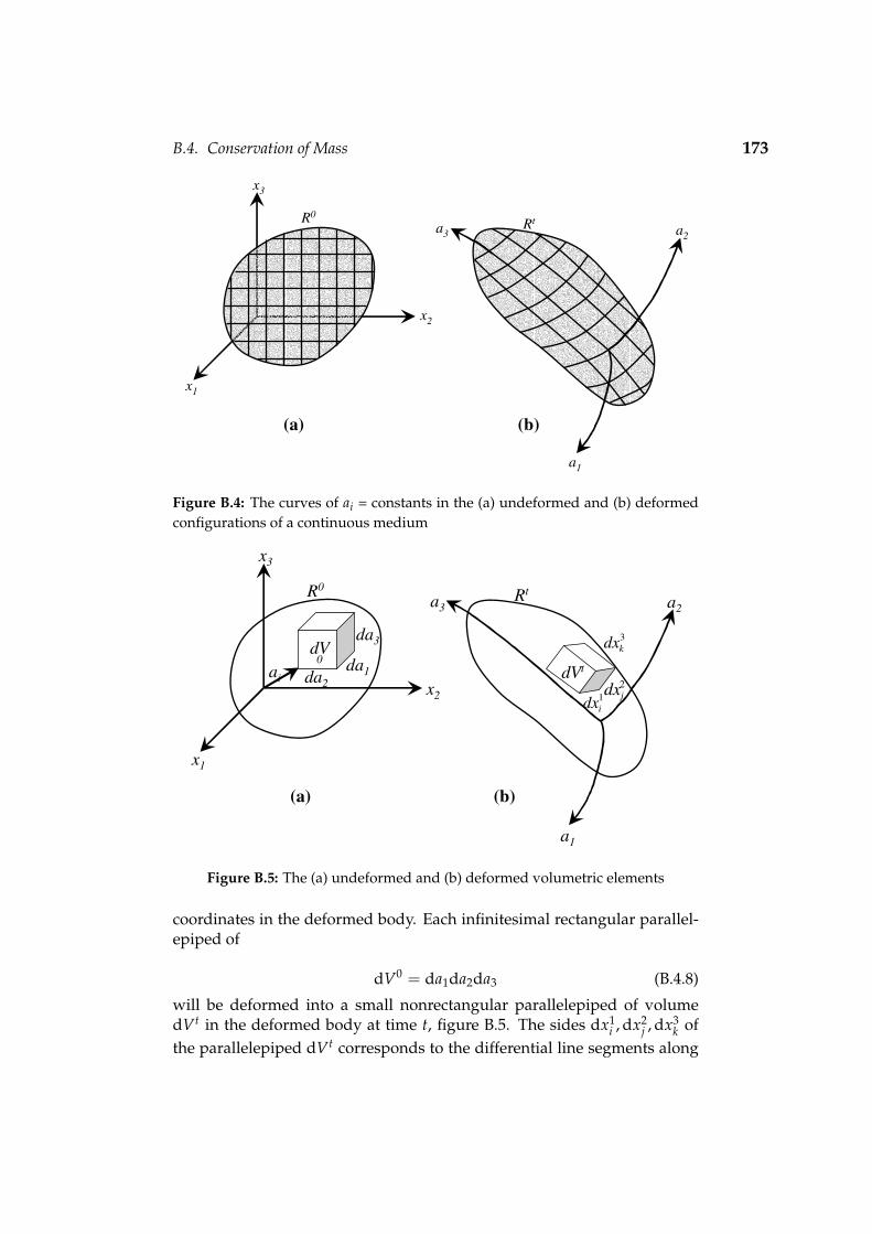
B.4. Conservation of Mass 173
x1
x2
x3
R0
a1
a2a3
Rt
(a) (b)
Figure B.4: The curves of ai = constants in the (a) undeformed and (b) deformedconfigurations of a continuous medium
x1
x2
x3
R0
(a)
aida1da2
da3dV0
a1
a2a3Rt
(b)
dVt
1idx
3kdx
2jdx
Figure B.5: The (a) undeformed and (b) deformed volumetric elements
coordinates in the deformed body. Each infinitesimal rectangular parallel-epiped of
dV0 = da1da2da3 (B.4.8)
will be deformed into a small nonrectangular parallelepiped of volumedVt in the deformed body at time t, figure B.5. The sides dx1
i , dx2j , dx3
k ofthe parallelepiped dVt corresponds to the differential line segments along

B.4. Conservation of Mass 174
the curvilinear coordinates in the deformed body, owing to the differentialchanges
dx1i =
∂xi
∂a1da1, dx2
j =∂xj
∂a2da2, dx3
k =∂xk
∂a3da3 (B.4.9)
The volume of the parallelepiped dVt can be shown to be
dVt = ε ijk∂xi
∂a1da1
∂xj
∂a2da2
∂xk
∂a3da3
= Jda1da2da3
(B.4.10)
where
J =∂(x1, x2, x3)∂(a1, a2, a3)
= ε ijk∂xi
∂a1
∂xj
∂a2
∂xk
∂a3
=
∣∣∣∣∣∣∣∂x1∂a1
∂x2∂a1
∂x3∂a1
∂x1∂a2
∂x2∂a2
∂x3∂a2
∂x1∂a3
∂x2∂a3
∂x3∂a3
∣∣∣∣∣∣∣(B.4.11)
is called the Jacobian of transformation of xi with respect to ai. Since themass contained in R0 should be identically the same as that in Rt, the fol-lowing integral continuity equation using Lagrangian description must bevalid ∫
Rtρ (a1, a2, a3, t) dVt =
∫R0
ρ (a1, a2, a3, 0) dV0 (B.4.12)
or ∫R0
ρ (a1, a2, a3, t) J dV0 =∫
R0ρ (a1, a2, a3, 0) dV0 (B.4.13)
But this equation should hold true for any region R0. Therefore
ρ (a1, a2, a3, t) J = ρ (a1, a2, a3, 0) (B.4.14)
Equation B.4.12 implies that the quantity ρ (a1, a2, a3, t) J is independent oftime for a given particle, or ai. Therefore the comoving derivative of ρJmust vanish
ddt
[ρ (a1, a2, a3, t) J] = 0 (B.4.15)
This is a differential continuity equation from the Lagrangian viewpoint.

B.5. Momentum Balance Principles 175
x1
x3
x2O
dV
vi
dS vi
niS
R
σ i
fi
xi
xj
Figure B.6: Free body diagram of an arbitrary region in space in which a conti-nuum moves
B.5 Momentum Balance Principles
The momentum principle for a collection of particles states that the timerate of change of the total momentum of a given set of particles equals thevector sum of all the external forces acting on the particles of the set, provi-ded Newton’s Third Law of action and reaction governs the internal forces.The continuum form of this principle is a basic postulate of continuum me-chanics.
B.5.1 Eulerian Description
Consider a given mass of the medium, instantaneously occupying a regionR bounded by surface S (as in figure B.6) and acted upon by a stress vectorσi and body force fi. If σi(xi, t) is acting on a surface element dS on S, ρ(xi)is the density of the volumetric element dV in region R, and fi(xi, t) is thebody force per unit mass of the same volumetric element; then Cauchy’sfirst law of motion becomes∫
Sσi dS +
∫R
ρ fi dV =∫
Rρ
dvi
dtdV (B.5.1)
where vi(xi, t) is the velocity vector at a point in the continuum. Using theReynolds transport theorem (Appendix A), equation B.5.1 becomes∫
Sσi dS +
∫R
ρ fi dV =∫
R
∂ (ρvi)∂t
dV +∫
Sρvivjnj dS (B.5.2)

B.5. Momentum Balance Principles 176
where ni(xi) is the unit normal vector to the surface element dS on S. Ex-pressing σi in terms of the stress tensor σij, we can rewrite equation B.5.2as
∫S
σijnj dS +∫
Rρ fi dV =
∫R
∂ (ρvi)∂t
dV +∫
Sρvivjnj dS (B.5.3)
This is called the momentum integral equation governing the motion of thecontinuum through the control volume. Transforming the surface integralsin equation B.5.3 to a volume integral using Gauss’ theorem yields∫
R
[σij,j + ρ fi −
∂ (ρvi)∂t
−(ρvivj
),j
]dV = 0 (B.5.4)
This equation should hold true for any arbitrary region of the continuumin motion, which means that the integrand on the left side should be iden-tically equal to zero, or
∂ (ρvi)∂t
+(ρvivj
),j = ρ fi + σij,j (B.5.5)
This is one form of the equation of motion. An alternative form can beobtained by first rewriting equation B.5.5 as follows[
vi∂ρ
∂t+ ρ
∂vi
∂t
]+[vi(ρvj)
,j + ρvjvi,j
]= ρ fi + σij,j
∴ vi∂ρ
∂t+ vi
(ρvj)
,j + ρ∂vi
∂t+ ρvjvi,j = ρ fi + σij,j
(B.5.6)
Multiplying the continuity equation, equation B.4.3 by vi yields
vi∂ρ
∂t+ vi (ρvi),i = 0 (B.5.7)
Equation B.5.7 corresponds to the first two terms in equation B.5.6, whichon substitution yields
ρ∂vi
∂t+ ρvjvi,j = ρ fi + σij,j (B.5.8)
Further note that the comoving derivative of the velocity vector vi is
dvi
dt=
∂vi
∂t+
∂vi
∂xj
dxj
dt=
∂vi
∂t+ vjvi,j (B.5.9)
Thus, the left side of equation B.5.8 is just the product of ρ and the como-ving derivative of the velocity vector vi. The equation of motion becomes
ρdvi
dt= ρ fi + σij,j (B.5.10)

B.5. Momentum Balance Principles 177
In the special case of static equilibrium of the medium the acceleration dvidt
is zero and equation B.5.10 reduces to the partial differential equation ofequilibrium
ρ fi + σij,j = 0 (B.5.11)
Next the moment of momentum principle is considered. In a collection ofparticles whose interactions are equal, opposite, and co-linear forces, thetime rate of change of the total moment of momentum for the given collec-tion of particles is equal to the vector sum of the moments of the externalforces acting on the system. In the absence of distributed couples, we pos-tulate the same principle for a continuum.
Recall from elementary mechanics that the moment of any force Fi aboutthe origin O is the vector product of the position vector xi and the force Fi,or ε ijkxjFk, where ε ijk is the permutation symbol. Applying the momentequation to the free body diagram of figure B.6 gives rise to the followingequation
∫S
ε ijkxjσk dS +∫
Rε ijkxj fkρ dV =
ddt
∫R
ρε ijkxjvk dV (B.5.12)
Substituting σk = σkrnr from equation B.2.8 yields
∫S
ε ijkxjσkrnr dS +∫
Rε ijkxj fkρ dV =
ddt
∫R
ε ijkxjρvk dV (B.5.13)
The surface integral in equation B.5.13 can be reduced to a volume integralby using Gauss’ theorem∫
Sε ijkxjσkrnr dS =
∫R
(ε ijkxjσkr
),r dV
=∫
Rε ijk(xj,rσkr + xjσkr,r
)dV
=∫
Rε ijk(δjrσkr + xjσkr,r
)dV
=∫
Rε ijk(σkj + xjσkr,r
)dV
(B.5.14)
Hence, equation B.5.13 becomes
∫R
ε ijk(σkj + xjσkr,r
)dV +
∫R
ε ijkxj fkρ dV =ddt
∫R
ε ijkxjρvk dV
=∫
Rε ijkρ
(vjvk + xj
dvk
dt
)dV
(B.5.15)

B.5. Momentum Balance Principles 178
therofore
∫R
ε ijk
[σkj − ρvjvk + xj
(σkr,r + ρ fk − ρ
dvk
dt
)]dV = 0 (B.5.16)
Noting that ε ijkvjvk = 0, since vjvk is symmetric in the indices jk while ε ijkis antisymmetric and that
σkr,r + ρ fk − ρdvk
dt= 0
is the equation of motion (equation B.5.10). Thus, equation B.5.16 reducesto ∫
Rε ijkσkj dV = 0 (B.5.17)
Again this equation should hold true for any arbitrary region R of the con-tinuum, which results in
ε ijkσkj = 0 (B.5.18)
This is the equation of angular momentum for a classic continuum. In ex-panded form equation B.5.18 becomes
for i = 1 σ32 − σ23 = 0for i = 2 σ13 − σ31 = 0for i = 3 σ21 − σ12 = 0
(B.5.19)
This establishes the symmetry of the stress tensor in general without anyassumption of equilibrium or of uniformity of the stress distribution.
B.5.2 Lagrangian Description
The Eulerian form of the linear momentum equation is given by equa-tion B.5.10.
ρdvi
dt= ρ fi + σij,j
where ρ = ρ (xi, t), fi = fi (xi, t), σi = σi (xi, t), vi (xi, t) = dxidt . Using the
rules to convert from the Eulerian to the Lagrangian description (AppendixA), we have
dvi (xi, t)dt
=∂vi (ai, t)
dt=
∂2ui (ai, t)∂t2 (B.5.20)
∂σij (xi, t)∂xi
=∂σij (ai, t)
∂ai(B.5.21)

B.6. Strain Tensor 179
We can also express the Eulerian functions ρ and fi in terms of the Lagran-gian coordinates, i.e.
ρ (xi, t) = ρ (ai, t)fi (xi, t) = fi (ai, t)
(B.5.22)
Therefore, the equation of linear momentum can be written as
ρ∂2ui
∂t2 = ρ fi + σij,j (B.5.23)
where all functions are expressed in terms of the Lagrangian coordinates aiand time t, and the subscript “,i” means ∂
∂ai. The equation of angular mo-
mentum, equation B.5.18, is formulated in the Eulerian description. Usingthe same rules, this equation in the Lagrangian description becomes
ε ijkσkj = 0 (B.5.24)
where σkj = σkj(ai, t).
B.6 Strain Tensor
As the continuum moves from one configuration to another, the matter inthe neighbourhood of each point is translated and rotated as a rigid body,and strained. Strain of an elemental volume is that part of the relative mo-tion between neighbouring particles that is not due to rigid body motion.
B.6.1 General or Finite Strain
This is the strain that occurs in the medium when no restrictions are placedon the magnitude of the displacements or derivatives of the displacementwith respect to position. The latter are called displacement gradients.
Eulerian Nonlinear Strain Tensor
Let P and Q be two neighbouring points in the medium before deforma-tion, at time = 0. After a given motion, at time = t, these two points moveto new positions p and q (figure B.7).
Using the Eulerian description, the vectors to the points can be writtenas follows
P : ai
Q : ai + dai
p : xi = ai + ui (xi, t)q : xi + dxi = ai + dai + ui (xi + dxi, t)
(B.6.1)

B.6. Strain Tensor 180
x1
x3
x2
Q
P
q
pxi
xi+dxi
ai+dai
ai
dai
ui(xi,t)
ui(xi+dxi,t)
dxi
time = 0 time = t
Figure B.7: Relative displacements between two neighbouring points in a conti-nuum
where ui (xi, t) and ui (xi + dxi, t) are the displacement vectors of P andQ respectively. The relative displacement vector between Pand Q after agiven deformation at a given time t is therefore the difference of the displa-cement vectors uQ
i and uPi of the two points.
dui = uQi − uP
i = ui (xi + dxi, t)− ui (xi, t) (B.6.2)
Assuming that the conditions that guarantee the existence of a derivativeare met, the differential dui can be written as
dui =(
∂ui
∂xj
)p
dxj (B.6.3)
where the partial derivatives are evaluated at point p and at time t. As themedium moves as a result of the displacements, the volumetric element inthe neighbourhood of P will translate and rotate as a rigid body and bestrained. To distinguish between the local rigid body motion and straining,compute the difference of the square of the differential lengths between p,q and P, Q. This is done because mathematically it is more convenient todiscuss than the difference of the same lengths. The squares of the lengthsare
|PQ|2 = (da)2 = daidai
|pq|2 = (dx)2 = dxidxi(B.6.4)

B.6. Strain Tensor 181
Therefore
(dx)2 − (da)2 = dxidxi − daidai (B.6.5)
At a given time t, the differential vector dai due to the difference of theposition vectors at P and Q can be expressed as follows
dai =(
∂ai
∂xj
)p
dxj (B.6.6)
where the partial derivative is again evaluated at point p and at time t.Equation B.6.5 becomes
(dx)2 − (da)2 = dxidxi − daidai
= dxidxi −∂ar
∂xidxi
∂ar
∂xjdxj
= dxi(δijdxj
)− ∂ar
∂xidxi
∂ar
∂xjdxj
=[
δij −∂ar
∂xi
∂ar
∂xj
]dxidxj
(B.6.7)
From the third equation in equation B.6.1 it follows that
xi = ai + ui (xi, t) ⇔ ai = xi − ui (xi, t) (B.6.8)
Substituting this expression into the last of equation B.6.7 yields
(dx)2 − (da)2 =[
δij −∂ar
∂xi
∂ar
∂xj
]dxidxj
=[
δij −∂
∂xi(xr − ur)
∂
∂xj(xr − ur)
]dxidxj
=[
δij −(
δri −∂ur
∂xi
)(δrjxr −
∂ur
∂xj
)]dxidxj
=[
δij − δij + δri∂ur
∂xj+ δrj
∂ur
∂xi− ∂ur
∂xi
∂ur
∂xj
]dxidxj
=[
∂ui
∂xj+
∂uj
∂xi− ∂ur
∂xi
∂ur
∂xj
]dxidxj
(B.6.9)
This equation can now be written as
(dx)2 − (da)2 = 2Eijdxidxj (B.6.10)
where
Eij =12
[∂ui
∂xj+
∂uj
∂xi− ∂ur
∂xi
∂ur
∂xj
](B.6.11)

B.6. Strain Tensor 182
is defined as the Eulerian nonlinear strain tensor. It is clear that the straintensor as given by equation B.6.11 is symmetrical.
Lagrangian Nonlinear Strain Tensor
Following the same procedure used in the preceding discussion, but usingai as the independent coordinates instead of xi, we obtain the displacementvector
ui = ui (ai, t) (B.6.12)
and the differential dui becomes
dui =(
∂ui
∂aj
)P
daj (B.6.13)
The Lagrangian nonlinear strain tensor then becomes
Lij =12
[∂ui
∂aj+
∂uj
∂ai+
∂ur
∂ai
∂ur
∂aj
](B.6.14)
B.6.2 Infinitesimal Strain
Infinitesimal strain tensors are characterised by small displacement gradi-ents, i.e. ∂ui
∂xj<< 1 in the Eulerian description and ∂ui
∂aj<< 1 in the Lagran-
gian description.
Eulerian Linear Strain Tensor
Assuming the derivatives of the displacements to be small, the term invol-ving the product of these derivatives in equation B.6.9 can be neglected incomparison with the other two terms, so that
(dx)2 − (da)2 =[
∂ui
∂xj+
∂uj
∂xi
]dxidxj (B.6.15)
We now define the Eulerian linear strain tensor
eij =12
[∂ui
∂xj+
∂uj
∂xi
](B.6.16)
so that equation B.6.15 can be written as
(dx)2 − (da)2 = 2eijdxidxj (B.6.17)
It should be emphasised that in the derivation given above, the assumptionthat the displacements are infinitesimal has not been used. The linear straintensor eij is also symmetric and follows the usual law of transformation

B.6. Strain Tensor 183
for a second order Cartesian tensor. Let us now derive an expression forthe change of length per unit of final length (length after deformation) forthe line element pq (figure B.7). Introducing the symbol e as the change inlength per unit of final length, this becomes
e =dx− da
dx(B.6.18)
Factoring the left side of equation B.6.17 as follows
(dx + da) (dx− da) = 2eijdxidxj (B.6.19)
and using the assumption of small changes of length (dx + da) ≈ 2dx,equation B.6.19 becomes
2dx (dx− da) = 2eijdxidxj
∴(dx− da)
dx= eij
dxi
dxdxj
dx
(B.6.20)
Substitution in equation B.6.18 yields
e = eijninj (B.6.21)
where
ni =dxi
dx(B.6.22)
are the direction cosines of the line element pq.
Lagrangian Linear Strain Tensor
Following the same procedure as in the preceding section, the terms in-volving the product of displacement gradients can be ignored so that theequivalent of equation B.6.15 can be written as
(dx)2 − (da)2 =[
∂ui
∂aj+
∂uj
∂ai
]daidaj (B.6.23)
We now define the Lagrangian linear strain tensor
lij =12
(∂ui
∂aj+
∂uj
∂ai
)(B.6.24)
so that equation B.6.23 becomes
(dx)2 − (da)2 = 2lijdaidaj (B.6.25)

B.6. Strain Tensor 184
The tensor lij is also symmetric and follows the usual law of transformationfor a second order Cartesian tensor. The change of length per unit initiallength for the line PQ can be shown to be
l =dx− da
da= lij
dai
dadaj
da= lijninj (B.6.26)
B.6.3 The Linear Rotation Tensor and Rotation Vector
Our studies of the roles of the rotation tensor and vector will be restrictedto the case of the infinitesimal displacement gradients only.
Eulerian Description
Earlier it was established that the relative displacement of two neighbou-ring points, P and Q, using the Eulerian description, is (equation B.6.3)
dui =(
∂ui
∂xj
)p
dxj (B.6.27)
where it is understood that the partial derivatives are to be evaluated at pand at time t. Equation B.6.27 can be written as the sum of a symmetricpart and a antisymmetric part
dui =[
12
(∂ui
∂xj+
∂uj
∂xi
)+
12
(∂ui
∂xj−
∂uj
∂xi
)]dxj (B.6.28)
Define the Eulerian linear rotation tensor
wij =12
(∂ui
∂xj−
∂uj
∂xi
)(B.6.29)
and equation B.6.27 can be written as
dui =[eij + wij
]dxj (B.6.30)
If a given set of displacements constitute rigid body motion, then the eij = 0everywhere. The converse is also true. Hence, the necessary and sufficientcondition of the continuum to have no straining in the vicinity of a point pis that eij = 0. Study the relative displacement of q with respect to p for thiscase. Equation B.6.30 then becomes
dui = wijdxj (B.6.31)

B.6. Strain Tensor 185
This should represent the displacement of q relative to p due to an infinite-simal rigid body rotation of the vector dxi only. The tensor wij is antisym-metric, i.e.
w11 = w22 = w33 = 0w23 = −w32
w13 = −w31
w12 = −w21
(B.6.32)
This means that the entire rotation tensor can be defined by three inde-pendent components. The following notation is introduced for these threecomponents
w1 = w32 = −w23
w2 = w13 = −w31
w3 = w21 = −w12
(B.6.33)
The three components of wi forms a vector called the Eulerian linear rota-tion vector. Equations B.6.32 and B.6.33 imply that the rotation vector wi isexpressible in terms of the rotation tensor
2wi = ε ijkwkj (B.6.34)
or inversely
wji = ε ijkwk (B.6.35)
Furthermore, upon substitution of the linear rotation tensor, equation B.6.29,into equation B.6.34, the three components of the rotation vector can beshown to be identical to the components of one-half the curl of the displa-cement vector
wi = 12 ε ijkuk,j (B.6.36)
Lagrangian Description
Thus far, only the Eulerian description has been used. It is obvious thatthe same discussion may be applied to the relative displacement using theLagrangian description referring everything to the undeformed length PQand the coordinates ai. Here, dui becomes
dui =[lij + wij
]daj (B.6.37)
where
lij =12
(∂ui
∂aj+
∂uj
∂ai
)(B.6.38)

B.6. Strain Tensor 186
is the linear Lagrangian strain tensor defined earlier and
wij =12
(∂ui
∂aj−
∂uj
∂ai
)(B.6.39)
is called the Lagrangian linear rotation tensor. The corresponding rotationvector is
2wi = ε ijkwkj (B.6.40)
or inversely
wji = ε ijkwk (B.6.41)
Furthermore, these components can also be written as the components ofone-half the curl of the displacement vector
wi = 12 ε ijkuk,j (B.6.42)
where
w11 = w22 = w33 = 0w23 = −w32
w13 = −w31
w12 = −w21
(B.6.43)
and
w1 = w32 = −w23
w2 = w13 = −w31
w3 = w21 = −w12
(B.6.44)
Except that the coordinates xi are replaced by ai, all properties and mea-nings assigned to the Eulerian rotation tensor and vector hold for the Lag-rangian rotation tensor and vector. Finally, under the assumption of infini-tesimal displacement gradients, it follows that
wij ≈ wij
lij ≈ eij(B.6.45)
Hence, the Eulerian description should yield approximately the same resultas the Lagrangian description.

B.6. Strain Tensor 187
22
1 xdxu
∂∂
22
2 xdxu
∂∂y1
y2
y3
P
Q
R
α23
22
3 xdxu
∂∂
Undeformed
(a) (b) (c)
p
q
r
Deformed
dx2
dx3p
q
Deformed
y3y3
y2
y1y1
y2
Figure B.8: (a) Line segment pq in the y1 direction (b) Undeformed and (c) defor-med states of two line segments finally orientated in the y2- and y3-directions
B.6.4 Geometrical Meanings of the Linear Strain Tensors
Eulerian Description
The Eulerian linear strain tensor is given by equation B.6.16.
eij =12
[∂ui
∂xj+
∂uj
∂xi
](B.6.46)
Also the change of length per unit of final length of a line element is (equa-tion B.6.21).
e = eijninj (B.6.47)
and the relative displacement of q with respect to p (equation B.6.27)
dui =(
∂ui
∂xj
)P
dxj (B.6.48)
These three equations will now be used to give a geometrical or physicalmeaning to the components of strain. Let us first obtain a physical meaningof the diagonal components e11, e22 and e33. To begin, take the differentialline segment pq in the x1-direction, or along the y1-(local) axis, as shown inFig. B.8a. The direction cosines for this element are
ni = (1, 0, 0) (B.6.49)
Substituting these into equation B.6.47 yields
e = e11 (B.6.50)

B.6. Strain Tensor 188
Therefore, e11 is the change of length per unit of original length of a dif-ferential line segment in the y1-direction. Similarly, it can be shown thate22 and e33 are changes of length per unit length of the differential line seg-ments drawn from p along the y2- and y3-directions respectively. Next, letsinvestigate the e23 off-diagonal element of the linear strain tensor as an ex-ample of all the off-diagonal elements.
Figures B.8b and B.8c show two sets of local Cartesian coordinates. Thevector yi has its origin at P in the undeformed body and the second yi hasits origin at p, the point to which the particle at P moves after deformation.Both sets are parallel to the global xi-axes. A line segment pq after defor-mation along the y2-axis has components of (0, dx2, 0), and the relativedisplacement of q with respect to Q after deformation has the components
dui =∂ui
∂xjdxj ⇒
(∂u1
∂x2dx2,
∂u2
∂x2dx2,
∂u3
∂x2dx2
)(B.6.51)
The size of this vector is approximately
|dui| =
√(∂u1
∂x2dx2
)2
+(
∂u2
∂x2dx2
)2
+(
∂u3
∂x2dx2
)2
≈ dx2 (B.6.52)
Therefore, to the lowest order, the components of a unit vector in the direc-tion of the undeformed line segment PQ are approximately as follows(
∂u1
∂x2, 1,
∂u3
∂x2
)(B.6.53)
In the same way, if we consider a differential line segment pr after defor-mation in the y3-direction, it will have components in the deformed stateof (0,0,dx3). The unit vector along the line element PR in the undeformedstate has the components (
∂u1
∂x3,
∂u2
∂x3, 1)
(B.6.54)
Hence, to the lowest order, the cosine of the angle α23 between the twoundeformed line segments PQ and PR is given by taking the dot productof the two unit vectors specified by equation B.6.53 and B.6.54. Thus,
cos α23 =∂u1
∂x2
∂u1
∂x3+
∂u2
∂x3+
∂u3
∂x2
≈ ∂u2
∂x3+
∂u3
∂x2= 2e23
(B.6.55)
B.7. Principal Strains and Principal Axes 189
Let the increase from the angle α23 in the undeformed state to the rightangle in the deformed state between the two differential line segments beβ23. Then
β23 = π2 − α23 (B.6.56)
But in the infinetesimal theory, β23 is very small, so that
β23 ≈ sin β23 = cos α23 (B.6.57)
Therefore, the difference in angle between the two line segments is
β23 = 2e23 = 2e32 and alsoβ13 = 2e13 = 2e31
β13 = 2e13 = 2e31
(B.6.58)
The three strain tensor components e23, e31, and e12, are thus equal to one-half the change of angle between two line segments that lie along the yi-directions in the deformed medium.
Lagrangian Description
The same procedures can be used to demonstrate the geometrical mea-nings of the components of the Lagrangian linear strain tensor. The dia-gonal components of the strain tensor l11, l22 and l33 can be shown to bethe change of length per unit original length of a differential line segmentoriginally in the y1, y2 and y3-directions respectively. The two line segmentsPQ and PR are assumed to be orthogonal and in the direction of the localy2 and y3-directions as depicted in figure B.9a.
Figure B.9b shows the two line segments in the deformed state. Usingthe relative displacements depicted in figure B.9 and following the sameprocedures as in the previous section, it follows that
β23 = 2l23 = 2l32
β13 = 2l13 = 2l31
β12 = 2l12 = 2l21
(B.6.59)
The three tensor strain components l23, l31 and l12 are thus equal to one-halfthe change of angle between two line segments originally 90 apart alongthe directions indicated by the numerical subscripts. These are one-half thefamiliar “shearing strains” as defined in a course in strength of materials.
B.7 Principal Strains and Principal Axes
In this section the principal axis theory for the linear strain tensor is given.Consider a general movement of the continuum in the vicinity of a point

B.7. Principal Strains and Principal Axes 190
y1
y2
y3
(a)
P
Q
R
Undeformed
da2
da3
22
1 adau
∂∂
22
2 adau
∂∂
p
q
r
α23
22
3 ada
u
∂∂
Deformed
(b)
y1
y2
y3
Figure B.9: (a) Undeformed and (b) deformed state of two line segments
P, which consists of straining and rigid body rotation and translation. Theeffects of rigid body rotation and straining can be studied separately andthen superimposed. In this section we shall consider the effects of purestrain only. Due to straining only, the displacement vector of a neighbou-ring point Q relative to P is
dui = lijdaj (B.7.1)
or the relative displacement of Q with respect to P per unit of originallength is a vector whose components are
li =dui
da= lijnj (B.7.2)
where da is the differential length PQ and nidai/da is the unit vector in thedirection of PQ. In general the relative displacement vector per unit lengthis not in the original direction of the line segment PQ, nor is it in the defor-med direction of the line segment pq. Following the same procedure thatwas used in defining principal directions for the stress tensor, define a prin-cipal direction for the strain tensor as an orientation of the line segment PQ forwhich the line element retains the property of perpendicularity to the sur-face of the particles originally in its perpendicular plane. Considering theeffects of strain only, this means that the relative displacement vector li perunit of length has the same direction as the original line element PQ. Thisshould not be confused with the idea of an invariant direction, for whenthe effects of rotation are added, the principal line elements will be rotatedfrom their original orientations. The magnitude of such a relative displace-ment per unit length (now a normal strain) is called a principal strain, and

B.8. The Linear Cubical Dilatation 191
the corresponding axis is called a principal axis of strain. By definition, forsuch a direction, the following equation must be satisfied
li = lni = lδijnj (B.7.3)
where l is the principal strain. Substituting for li from equation B.7.2, equa-tion B.7.3 becomes (
lij − lδij)
nj = 0 (B.7.4)
Furthermore, the components of the unit vector always satisfy nini = 1. Thenontrivial solution for ni in equation B.7.4 require that the determinant ofthe coefficients of the ni be equal to zero∣∣lij − lδij
∣∣ = 0 (B.7.5)
In general, equation B.7.5 will yield three values of l. These three principalstrains will be denoted by l1, l2 and l3. In the Eulerian description, theprincipal directions are defined as those for which the displacement vectorper unit length of deformed line due to pure strain
ei = eijnj (B.7.6)
is in the direction of the deformed segment. Stated in a different way, aprincipal direction is one for which the deformed line element retains theproperty of perpendicularity to the surface of particles originally in its per-pendicular plane. The direction cosines are ni. The magnitude of ei for aprincipal direction is a principal strain. Equations for determining this are(
eij − δije)
nj = 0
nini = 1(B.7.7)
where e is a principal strain. The principal values e1, e2 and e3 are given bythe following determinant ∣∣eij − eδij
∣∣ = 0 (B.7.8)
B.8 The Linear Cubical Dilatation
The cubical dilatation D, in the Eulerian description, is defined as the in-crease of volume per unit of final volume in the neighbourhood of a pointp in the continuum. Infinitesimal theory applies.
Consider a differential rectangular parallelepiped in the deformed me-dium with one corner at p. Let its three edges of lengths dx1, dx2 and dx3

B.9. Compatibility Equations for Linear Strain Components 192
coincide with the principal directions of strain. From the definition of D,the cubical dilatation of this parallelepiped is given by
D =Vdeformed −Vundeformed
Vdeformed
=dx1dx2dx3 − dx1 [1 + e(1)] dx2 [1 + e(2)] dx3 [1 + e(3)]
dx1dx2dx3
(B.8.1)
Neglecting terms involving product of e1, e2, e3 because of the infinitesimalassumption, D becomes
D = e1 + e2 + e3 = eii (B.8.2)
where eii is the first invariant of the Eulerian strain tensor. Therefore thefirst strain invariant eii in any coordinate system is the cubical dilatationD. In the Lagrangian description, the cubical dilatation D is defined asthe increase of volume per unit of original volume in the neighbourhoodof a point P in the continuum. Letting the three edges of the rectangularparallelepiped be da1, da2 and da3 and following the same procedure itfollows that
D = l1 + l2 + l3 = lii (B.8.3)
B.9 Compatibility Equations for Linear Strain Components
B.9.1 Eulerian Description
The symmetric Eulerian linear strain tensor given by equation B.6.16
eij =12
[∂ui
∂xj+
∂uj
∂xi
]is equivalent to six equations with the six independent components eij onthe one side and the three displacements ui on the other. If the strainsare determined first, we have six equations for the determining the threeunknown displacements ui. In general, a set of displacements for any ela-sticity problem will not exist unless the strains eij satisfy certain conditi-ons. The equations that the strains components must satisfy in order thatthe displacements be single-valued and continuous are called compatibilityequations. They are both necessary and sufficient conditions.
We shall derive these equations and establish their necessity and suf-ficiency. Consider two points in a continuum whose coordinates are xi(1)

B.9. Compatibility Equations for Linear Strain Components 193
and xi(2), using the Eulerian description. We wish to compute the displa-cements ui(1), relative to ui(2), along some curve C joining the two points.If the displacement vector ui is single-valued and continuous, then
ui(2) = ui(1) +∫
Cdui (B.9.1)
where C is any continuous curve joining xi(1) and xi(2). But from equa-tion B.6.30
dui =[eij + wij
]dxj
Therefore
ui(2) = ui(1) +∫
Ceijdxj +
∫C
wijdxj (B.9.2)
For convenience in integrating, substitute d[xj − xj(2)
]for dxj in the se-
cond integral. This is an identity, for xj is any point on C, and xj(2) isconstant for the second end point. Hence,
ui(2) = ui(1) +∫
Ceijdxj +
∫C
wijd[xj − xj(2)
](B.9.3)
Using the technique of integration by parts on the second integral, it can beexpressed as
∫C
wijd[xj − xj(2)
]=[wij[xj − xj(2)
]](2)(1) −
∫C
[xj − xj(2)
]wij,k dxk
= −wij(1)[xj(1)− xj(2)
]−∫
C
[xj − xj(2)
]wij,k dxk
(B.9.4)But
wij,k = 12
(ui,j − uj,i
),k = 1
2
(ui,jk − uj,ik
)= 1
2
(ui,jk + uk,ij
)− 1
2
(uj,ik + uk,ij
)= eik,j − ejk,i
(B.9.5)
Hence the integral of equation B.9.4 can be written as
∫C
wijd[xj − xj(2)
]= −wij(1)
[xj(1)− xj(2)
]+∫
C
[xj − xj(2)
] (ejk,i − eik,j
)dxk
(B.9.6)Thus, substituting equation B.9.6 into equation B.9.3, it becomes
ui(2) = ui(1)+∫
Ceikdxk−wij(1)
[xj(1)− xj(2)
]+∫
C
[xj − xj(2)
] (ejk,i − eik,j
)dxk
(B.9.7)

B.9. Compatibility Equations for Linear Strain Components 194
or
ui(2) = ui(1)− wij(1)[xj(1)− xj(2)
]+∫
CFikdxk (B.9.8)
where
Fik = eik +[xj − xj(2)
] (ejk,i − eik,j
)(B.9.9)
Since the displacement vector is single-valued and continuous, the integral∫C Fikdxk must be independent of the path of integration. In other words,
the integral should yield the same result for any continuous curve C joiningxi(1) and xi(2). Hence there must exist three functions Gi(x) that are single-valued and have continuous derivatives such that
Fikdxk = dGi = Gi,kdxk (B.9.10)
This means that
Fik = Gi,k (B.9.11)
But the functions Gi have continuous derivatives through the second-orderedones, so the necessary and sufficient conditions that the ui can be calculatedare
Gi,kl = Gi,lk (B.9.12)
and therefore
Fik,l = Fil,k (B.9.13)
Writing equation B.9.13 in terms of the strain components, we obtain
eik,l +[xj − xj(2)
] (ejk,il − eik,jl
)+(ejk,i − eik,j
)δjl
= eil,k +[xj − xj(2)
] (ejl,ik − eil,jk
)+(ejl,i − eil,j
)δjk (B.9.14)
in this equation all terms containing derivatives of strain alone or with theKronecker delta as a coefficient cancel, leaving the following[
xj − xj(2)] (
ejk,il + eil,jk − eik,jl − ejl,ik)
= 0 (B.9.15)
Equation B.9.15 holds for any arbitrary point xi. Consequently, the coeffi-cient of
[xj − xj(2)
]must vanish. Thus, a necessary and sufficient condition
for the displacement vector ui to be single-valued and continuous is
eik,jl + ejl,ik = ejk,il + eil,jk (B.9.16)
B.10. The Rate of Strain Tensor and the Vorticity Tensor 195
or by interchanging the indices j and k
eij,kl + ekl,ij = ejk,il + eil,jk (B.9.17)
where the symmetry property of the strain tensor has been used in the firstterm on the right-hand side and the order of the differentiation has beenchanged in the last. For the final form, the indices i and j on the right-handside of equation B.9.17 are switched, and the same properties are used againon the left side. Thus
eij,kl + ekl,ij = eik,jl + ejl,ik (B.9.18)
Equation B.9.18 represents a set of 34 = 81 equations. They are called thecompatibility equations for the linear strain components in the Eulerian de-scription. Of these 81 equations only 6 are independent. The numericalchoices for the indices for the independent equations are the following
i : 1 3 2 1 2 3j : 1 3 2 1 2 3k : 2 1 3 2 3 1l : 2 1 3 3 1 2
(B.9.19)
B.9.2 Lagrangian Description
Using the Lagrangian linear strain tensor lij, the same discussion will hold
true for the Lagrangian description, provided that ∂ui(ai ,t)∂aj
<< 1. With thisrestriction, the compatibility equations are
lij,kl + lkl,ij = lik,jl + ljl,ik (B.9.20)
B.10 The Rate of Strain Tensor and the Vorticity Tensor
The stress required to deform a medium may be some function of the ma-gnitudes of the strains and the rate at which the deformation takes place.The exact functional relationship varies from material to material. In a pu-rely elastic solid, rates of straining are not important, whereas the stressesin a fluid depend mainly upon the rates of strain. In this section, we shallbe interested primarily in the rate at which deformation takes place.
Introduce the Eulerian velocity field vi(xi,t) of each particle of the con-tinuum as a function of its instantaneous position and time. Consider agiven instance in time t. At this instant, the velocity of a particle p in thedeformed medium is vi, figure B.10. Consider the variation of velocity dueto position only, the velocity of a neighbouring particle q, where the vector
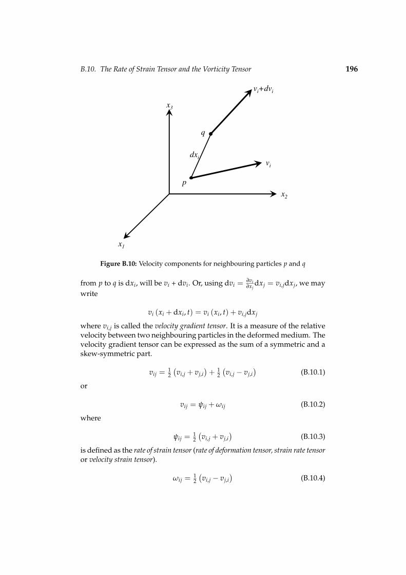
B.10. The Rate of Strain Tensor and the Vorticity Tensor 196
x1
x2
x3
p
q
dxivi
vi+dvi
Figure B.10: Velocity components for neighbouring particles p and q
from p to q is dxi, will be vi + dvi. Or, using dvi = ∂vi∂xj
dxj = vi,jdxj, we maywrite
vi (xi + dxi, t) = vi (xi, t) + vi,jdxj
where vi,j is called the velocity gradient tensor. It is a measure of the relativevelocity between two neighbouring particles in the deformed medium. Thevelocity gradient tensor can be expressed as the sum of a symmetric and askew-symmetric part.
vij = 12
(vi,j + vj,i
)+ 1
2
(vi,j − vj,i
)(B.10.1)
or
vij = ψij + ωij (B.10.2)
where
ψij = 12
(vi,j + vj,i
)(B.10.3)
is defined as the rate of strain tensor (rate of deformation tensor, strain rate tensoror velocity strain tensor).
ωij = 12
(vi,j − vj,i
)(B.10.4)

B.11. The Rate of Rotation Vector and the Vorticity Vector 197
is called the vorticity tensor. The velocity of q relative to p, or dvi, can bewritten as
dvi = vi (xi + dxi, t)− vi (xi, t) =(ψij + ωij
)dxj (B.10.5)
Let us now relate the rate of strain tensor ψij to the Eulerian linear straintensor eij and the vorticity tensor ωij to the rotation tensor wij. The linearstrain tensor follows from equation B.6.16
eij =12[ui,j + uj,i
]Now take the comoving derivative of both sides
deij
dt=
12
(ddt
ui,j +ddt
uj,i
)(B.10.6)
But duidt = vi are the Eulerian velocity components. Upon interchanging the
order of differentiation on the right side of equation B.10.6 gives
deij
dt=
12
[(dui
dt
),j+(
duj
dt
),i
]= 1
2
(vi,j + vj,i
)= ψij (B.10.7)
In the same way it can be shown that
dwij
dt= ωij (B.10.8)
Thus, ψij and ωij are simply comoving derivatives of eij and wij respectively.Physically, ψijis a measure of the rate of straining, and ωij is the time rateof rigid body rotation for the medium in the neighbourhood of p.
B.11 The Rate of Rotation Vector and the Vorticity Vector
From the definition of the vorticity tensor, equation B.10.4
ωij = 12
(vi,j − vj,i
)which is a symmetric tensor, i.e.
ω11 = ω22 = ω33 = 0ω23 = −ω32
ω31 = −ω13
ω12 = −ω21
(B.11.1)

B.11. The Rate of Rotation Vector and the Vorticity Vector 198
Since there are only three independent components, this means that thecomponents of the vorticity tensor can be related to the components of avector as follows
ω1 = −ω23 = ω32
ω2 = −ω31 = ω13
ω3 = −ω12 = ω21
(B.11.2)
The vector ωi is called the rate of rotation vector. The rate of rotation vectorand the vorticity vector are related to the vorticity tensor as follows
2ωi = ζi = ε ijkωkj
ωji = ε ijkωk = 12 ε ijkζk
(B.11.3)
where ζi is called the vorticity vector, defined as twice the rate of rotationvector. The rate of rotation vector and the vorticity vector can also be rela-ted to the curl of the velocity field
2ωi = ζi = ε ijkvk,j (B.11.4)

Appendix C
Polar Continuum Mechanics
C.1 Introduction
In Appendix B we have assumed the nonpolar case with no distributedcouples (moments) on the boundary surface and internal surfaces and nobody couples. External couple distributions could result from the action ofan external magnetic field on magnetised particles of the material or the ac-tion of an electric field on polarised matter. Even without assigned externalcouples, couple-stress can arise from interactions between adjacent parts ofthe material other than central-force interactions.
We have considered only the force per unit area transmitted across asurface at a point and not a possible couple. When a continuous distribu-tion of force acts across a finite area ∆S, the resultant of the distributions, ingeneral, is a force and a couple. If the result is divided by ∆S and the limittaken as ∆S tends to zero, it is found that the couple per unit area producedat the point by the continuous distribution of force is zero. This does not, ofcourse, preclude the possibility that there might also be a continuous distri-bution of couple, whose limit (per unit area) would be different from zero,i.e. a couple-stress.
C.2 The Cosserat Equations
In a theory of deformation of continua by E. Cosserat and F. Cosserat in1909, the couple per unit area (couple-stresses), acting across a surface withina material volume or on its boundary, is taken into account in addition tothe usual force per unit area.
C.2.1 The Couple-Stress Tensor and Couple-Stress Vector
As in Appendix B.2, consider a planar surface area ∆S oriented by the unitnormal vector ni and containing the point P. This planar surface separatesa portion of a material volume R1 from the remainder R2. Let ∆Fi be thetotal force that the material on the +ni side exerts on the material on the –niside across the surface (figure C.1). In addition to the force, a total moment∆Mi is also exerted on the material. The moment vector ∆Mi is taken aspositive in the direction of advance of a right handed thread.
The stress vector at point P is defined by equation B.2.4. The couple-
199

C.2. The Cosserat Equations 200
R1
R2
P∆S
ni
∆Fi
x2
x1
x3
∆Mi
Figure C.1: Resultant force and couple acting on area ∆S
x2σ22
σ32
σ12σ21
σ31
σ11
σ23
σ13
σ33
)1(iσ
)2(iσ
)3(iσ
x1
x3
)3(iµ
)2(iµ
)1(iµ
x1
x2
x3
µ21
µ31
µ11
µ22
µ32
µ12
µ23
µ33
µ13
+
Figure C.2: (a) Stress vectors and stress tensor components (b) Couple-stress vec-tors and couple-stress components

C.2. The Cosserat Equations 201
stress vector (also at point P) is defined similarly
µi = lim∆S→0
∆Mi
∆S(C.2.1)
The Cauchy stress theorem relating the stress tensor σij and the stress vectorσi was shown to be
σi = σijnj (C.2.2)
An similar expression can be written that relates the couple-stress tensorµij and the couple-stress vector µi.
µi = µijnj (C.2.3)
To prove equation C.2.3, consider a point P in a continuum. Figure C.2ashows the stress vectors and stress tensor components as shown in Ap-pendix B and figure C.2b shows the couple-stress vectors and couple-stresstensor components. These two sets of stresses act simultaneously at pointP, but are shown separately to avoid confusion. Take the unit vector niof the surface containing point P to be in the direction of the x2-axis (theshaded surface in figure C.2b).
The couple-stress vector µi on this element is, in general, in some ar-bitrary direction, but may be resolved into three orthogonal components.The components of the couple-stress vector µ
(2)i are µ12, µ22 and µ32, where
the first subscript indicates the direction of the couple stress componentand the second subscript indicates the direction of the normal vector to thesurface. Similarly we can visualise two other couple-stress vectors µ
(1)i and
µ(3)i acting on surface elements whose normals are in the positive x1- and
x3-directions respectively. They have couple-stress components of µ11, µ21,µ31 and µ13, µ23, µ33 respectively. Consider a Cauchy tetrahedron at pointP, bounded by three coordinate planes and a sloping face normal to ni asshown in figure C.3. The local Cartesian coordinate system has its origin atP.
Figure C.3a shows the stress vectors acting on the four sides of the tetra-hedron and figure C.3b shows the couple-stress vectors acting on the sametetrahedron. Again these two sets of traction vectors act simultaneously onthe tetrahedron, but are shown separately to avoid confusion. The presenceof the couples does not affect the consideration of linear momentum, andthe relation between the stress vector and the stress tensor still holds
σi = σijnj (C.2.4)
We now apply the moment of momentum principle to the mass inside thetetrahedron. Couple-stresses and -forces acting on the tetrahedron are

C.2. The Cosserat Equations 202
+ni
P P2
P1
P3
x1
x2
x3
( ))1()1( ˆii µµ +−
( ))2()2( ˆ ii µµ +−
( ))3()3( ˆii µµ +−
(b)
ni
P P2
P1
P3
x1
x2
x3
( ))1()1( ˆii σσ +−
( ))2()2( ˆ ii σσ +−
( ))3()3( ˆii σσ +−
(a)
( )ii σσ ˆ+ ( )ii µµ ˆ+
Figure C.3: Small tetrahedron at point P with (a) stress vectors and (b) with cou-ple-stress vectors
µi = couple-stress vector at P acting across a small surface element whosenormal is ni
µij = couple-stress tensor at point P
ci = body-couple vector per unit massh = depth of tetrahedron measured from the sloping faceρ = density at point P
It is clear that average quantities must be introduced, since the tetrahedronis finite. Define the following average quantities:

C.2. The Cosserat Equations 203
µi + µi = average couple-stress vector
−(
µ(1)i + µ
(1)i
)= average couple-stress vector across surface
PP2P3 on the tetrahedron. The negative sign
appears because(
µ(1)i + µ
(1)i
)would denote
the average couple-stress vector on a surfacewhose outward normal pointed in the positivex1-direction. Couples are defined as positiveif the couple vector (axis vector according tothe right-hand-rule) points in the positiveaxis direction.
−(
µ(2)i + µ
(2)i
)= average couple-stress vector across surface
PP1P3 on the tetrahedron.
−(
µ(3)i + µ
(3)i
)= average couple-stress vector across surface
PP1P2 on the tetrahedron.ci + ci = average body couple per unit massρ + ρ = average density of the tetrahedron
The area of the sloping surface P1P2P3 is A and
limh→0
(µi, µij, ci, ρ
)= 0 (C.2.5)
As the altitude h will be allowed to approach zero so that the volume of thefour surface areas simultaneously approach zero, while the position of Pdoes not change. It follows that the average values will approach the localvalues at the point P, and the result will be an expression for the couple-stress vector µi at point P in terms of the other three special surface couple-stress vectors at P.
Suppose that the particles of the continuum may posses spin angular mo-mentum hc
i (per unit mass, i.e. kg·m2·s−1·kg−1 = m2·s−1). The expressionfor the total moment of momentum is derived in Appendix D, and the ex-
pression for hci is given in vector notation as h
−→c. The Eulerian moment of
momentum equation of the classical non-polar continuum, equation B.5.12∫S
ε ijkxjσk dS +∫
Rε ijkxj fkρ dV =
ddt
∫R
ε ijkxjρvk dV (C.2.6)

C.2. The Cosserat Equations 204
is extended in two ways. Firstly, the volume body moment ci per unit massand the surface moment per unit area µi are introduced in addition to themoments of the body force per unit mass fi and the surface force per unitarea σi. Secondly, include the spin angular momentum hc
i as described above.The angular momentum balance with reference to point P in figure C.3becomes
∫S
(ε ijkxjσk + µi
)dS +
∫R
ρ(ε ijkxj fk + ci
)dV =
ddt
∫R
ρ(ε ijkxjvk + hc
i)
dV (C.2.7)
With xj measured from the vertex of the tetrahedron, it is apparent thatfor non-vanishing µi, ci and hc
i and for finite σk, fk and vi the contributionsof the terms containing the cross products are of an order higher than theother terms as the altitude h of the tetrahedron tends to zero. We accordin-gly omit them now and apply the mean-value theorem of integral calculusto the integrals over the faces and the volume of the tetrahedron. We thusobtain
−(
µ(1)i + µ
(1)i
)(n1 A)−
(µ
(2)i + µ
(2)i
)(n2 A)−
(µ
(3)i + µ
(3)i
)(n3 A) +
(µi + µi) A + (ρ + ρ) (ci + ci)( 1
3 Ah)
= (ρ + ρ)dhc
idt( 1
3 Ah)
(C.2.8)
where PP2P3 = n1 A and according to equation A.5.28
ddt
∫R
ρhci dV =
∫R
ρdhc
idt
dV (C.2.9)
Now let h approach zero and noting that the conditions in equation C.2.5hold, equation C.2.8 becomes
µi = µ(1)i n1 + µ
(2)i n2 + µ
(3)i n3
∴ µi = µijnj(C.2.10)
where the couple-stress vector µi on an arbitrary plane is expressed in termsof the couple-stress on the coordinate planes through the point.
C.2.2 Momentum Balance Principles
Eulerian Description
The presence of the couple-stresses does not affect the linear momentumprinciple; hence the equations of motion of the nonpolar continuum, equa-

C.2. The Cosserat Equations 205
tion B.5.10, still applies
ρdvi
dt= ρ fi + σij,j (C.2.11)
where vi (xi, t) = dxidt . We must, however, reconsider the moment of mo-
mentum equation of the non-polar continuum, equation B.5.12
∫S
ε ijkxjσk dS +∫
Rε ijkxj fkρ dV =
ddt
∫R
ρε ijkxjvk dV (C.2.12)
Including the body couple, the surface couples and the spin angular mo-mentum, this equation becomes (equation C.2.7)
∫S
(ε ijkxjσk + µi
)dS +
∫R
ρ(ε ijkxj fk + ci
)dV =
ddt
∫R
ρ(ε ijkxjvk + hc
i)
dV (C.2.13)
Substituting σk = σkrnr and µi = µijnj yields
∫S
(ε ijkxjσkrnr + µijnj
)dS +
∫R
ρ(ε ijkxj fk + ci
)dV =
ddt
∫R
ρ(ε ijkxjvk + hc
i)
dV (C.2.14)
The surface integral can be reduced to a volume integral by applying Gauss’theorem
∫S
(ε ijkxjσkrnr + µijnj
)dS =
∫S
(ε ijkxjσkrnr
)dS +
∫S
(µijnj
)dS
=∫
R
(ε ijkxjσkr
),r dV +
∫R
(µij)
,j dV
=∫
Rε ijk(xj,rσkr + xjσkr,r
)dV +
∫R
µij,j dV
=∫
Rε ijk(δjrσkr + xjσkr,r
)dV +
∫R
µij,j dV
=∫
R
[ε ijk(σkj + xjσkr,r
)+ µij,j
]dV
(C.2.15)Hence equation C.2.14 becomes

C.2. The Cosserat Equations 206
∫R
[ε ijk(σkj + xjσkr,r
)+ µij,j
]dV +
∫R
ρ(ε ijkxj fk + ci
)dV
=ddt
∫R
ρ(ε ijkxjvk + hc
i)
dV
=∫
Rρ
[ε ijk
(vjvk + xj
dvk
dt
)+
dhci
dt
]dV
Thus,
∫R
[ε ijk
(σkj + xjσkr,r + ρxj fk − ρvjvk − ρxj
dvk
dt
)+ µij,j + ρci − ρ
dhci
dt
]dV = 0
Therefore
∫R
[ε ijk
(σkj + xj
(σkr,r + ρ fk − ρ
dvk
dt
)− ρvjvk
)+ µij,j + ρci − ρ
dhci
dt
]dV = 0
(C.2.16)
Noting that ε ijkvjvk = 0 and that
σkr,r + ρ fk − ρdvk
dt= 0
is the equation of linear motion, equation C.2.11, then equation C.2.16 re-duces to ∫
R
[ε ijkσkj + µij,j + ρci − ρ
dhci
dt
]dV = 0 (C.2.17)
Again this equation should hold true for any arbitrary region R of the con-tinuum which results in
ε ijkσkj + µij,j + ρci = ρdhc
idt
(C.2.18)
With σkj = σkj (xi, t), µij = µij (xi, t), ρ = ρ (xi, t), ci = ci (xi, t), hci =
hci (xi, t) and “,i” = ∂
∂xi. This is the Eulerian equation of angular momentum
for a polar continuum. It forms a set of three partial differential equationsexpressing the rotational momentum principle in the presence of couplestresses µij, body couples ci per unit mass, and spin angular momentumhc
i per unit mass. The Cauchy stress tensor σij is nonsymmetric in gene-ral, though symmetry could be retained if ci, µij and hc
i were to form anequilibrated system by themselves.

C.2. The Cosserat Equations 207
x1
x2
τµ
µ31
µ32
α
α
P
B
C
X1
X2
σ22
σ12
σ21
σ11
σ
Figure C.4: Non-symmetric stress and couple stress state in a Cosserat continuum
Lagrangian Description
The Lagrangian linear momentum equation still holds, equation B.5.23.
ρ∂2ui
∂t2 = ρ fi + σij,j (C.2.19)
where ρ = ρ (ai, t), fi = fi (ai, t), σij = σij (ai, t) and the subscript “,i” means∂
∂ai. The Eulerian angular momentum equation is given by equation C.2.18.
Using the rules to convert from the Eulerian to the Lagrangian description(Appendix A), equation C.2.18 can be written as
ε ijkσkj + µij,j + ρci = ρ∂hc
i∂t
(C.2.20)
where all functions are expressed in terms of the Lagrangian coordinates aiand time t.
C.2.3 Mohr’s Circle of Non-Symmetric Stress Tensor
It is well known that the stress acting on any plane through a point at whichthe stress components are known, can be calculated from the equationsof statics. This analysis leads to the Mohr circle representation. Considera plane stress or plane strain problem in the x1x2 plane. Let point P beany point in the continuum with the known stress and couple-stress com-ponents σ12, σ21, σ22, σ11, µ31, µ32 as depicted in figure C.4.

C.2. The Cosserat Equations 208
Take the plane BC parallel to the x3 axis, at a small distance from P, sothat this plane together with the two coordinate planes cuts out from thematerial a very small triangular prism PBC. Since the stresses vary conti-nuously over the volume of the body, the stresses acting on the plane BCwill approach the stresses on the parallel plane through P as the element ismade smaller. In discussing the conditions of equilibrium of a small trian-gular prism, the body force and body moment can be neglected as a smallquantity of a higher order.
Note that this is not the case when the equilibrium equation of a smallvolumetric cubic is considered for the derivation of the momentum balanceprinciples (section C.2.2). This is because the body force and body momenthave the same order of magnitude as the terms owing to the variations ofthe stress components that are under consideration. The triangular prismis also assumed very small and the variation of the stresses over the sidescan be ignored and assumed to be uniformly distributed. If the area of sideBC is A, the area of BP can be shown to be A cos α and the area of side PCto be A sin α. If we denote by X1 and X2 the components of stress actingon the side BC, the equations of translational equilibrium of the prismaticalelement give
X1 = σ11 cos α + σ12 sin α
X2 = σ21 cos α + σ22 sin α(C.2.21)
The normal σ and shearing τ components of stress on plane BC can bewritten as
σ = X1 cos α + X2 sin α = σ11 cos2 α + σ22 sin2 α + (σ12 + σ21) sin α cos α
τ = X2 cos α− X1 sin α = σ21 cos2 α− σ12 sin2 α + (σ22 − σ11) sin α cos α(C.2.22)
The rotational equilibrium equation is
µ = µ32 sin α + µ31 cos α (C.2.23)
After some algebraic manipulation (Iordache and Willam, 1998), equation C.2.22can be written as
(σ− σc)2 + (τ − τc)
2 = r2 (C.2.24)
where
σc =σ11 + σ22
2, τc =
σ21 − σ12
2, r2 =
(σ11 − σ22
2
)2
+(
σ12 + σ21
2
)2

C.2. The Cosserat Equations 209
0 σc
σmin
σmax
C
(σ22, σ12)
(σ11, -σ21)τc
σ
τ
σ1 σ2
Figure C.5: Mohr’s circle of a non-symmetric state of stress
Equation C.2.24 represents a circle called the generalised Mohr’s circle asshown in figure C.5. Shear stress is taken positive in the upward direc-tion (figure C.5) and consider shear stresses as positive when they give acouple in the clockwise direction (figure C.4). This representation of thenon-symmetric state of stress in the Mohr plane, leads to a circle in twodimensions whose centre is no longer located on the σ-axis as is the casewith a non-polar continuum. The shift of the centre of the Mohr’s circle isa measure of the loss of symmetry. If the Mohr circle does not intersect theσ-axis, then there exist no real valued principal stresses. Setting τ = 0, inequation C.2.24, yields the following quadratic equation in σ
σ2 − 2σcσ +(σ2
c + τ2c − r2) = 0 (C.2.25)
Solving for the roots of σ
σ = 2σc ±√
4σ2c − 4 (σ2
c + τ2c − r2)
2
= 2σc ±
√(σ11 − σ22)
2 + 4σ12σ21
2
(C.2.26)
The principal normal stresses σ1 and σ2 (figure C.5) are real-valued only aslong as the discriminant is positive, i.e.
∆σ > 0 where ∆σ = (σ11 − σ22)2 + 4σ12σ21 (C.2.27)

C.3. Kinematics of Cosserat Continua 210
When ∆σ < 0, then the two eigenvalues turn complex, which correspondsto a Mohr circle that no longer intersects the σ-axis, and thus has no real-valued principal stresses. This can only happen if σ12 and σ21 have oppositesigns. In this context it is important to recall the Bromwich bounds (Iorda-che and Willam, 1998) according to which the eigenvalues of the symmetri-sed state enclose the lowest and highest eigenvalues of the non-symmetricstate of stress
σmin = σsym2 6 < (σ2) 6 < (σ1) 6 σ
sym1 = σmax (C.2.28)
For example, the non-symmetric state of stress
σij =[
1.5 0.30.7 0.5
](C.2.29)
has principal values σ1 = 1.678 and σ2 = 0.322, which are bound by themaximum and minimum values of the symmetrised stress state
σij =[
1.5 0.50.5 0.5
](C.2.30)
with principal values of σ1 = 1.707 and σ2 = 0.293. This elementary exam-ple illustrates that the real-valued maximum and minimum normal stressesbound the principal normal stresses of zero shear.
C.3 Kinematics of Cosserat Continua
The kinematics of micropolar continua are characterised by rotational de-grees of freedom wc
i → R3 , which are independent of the translatory mo-tion described by the displacement field ui. Thus the field of continuummacro-rotations does no longer coincide with that of micro-rotations ateach material particle, i.e. the micro-rotation wc
i differs from the classi-cal macro-rotation wi (equation B.6.34) since three rotational degrees-of-freedom are introduced in addition to the conventional three translationaldegrees-of-freedom. Assign a local rigid triad to every material point of thecontinuum body.
The symmetric linear strain tensor is given by equation B.6.16
eij =12
(∂ui
∂xj+
∂uj
∂xi
)(C.3.1)
and the skew-symmetric linear rotation tensor by equation B.6.29
wij =12
(∂ui
∂xj−
∂uj
∂xi
)(C.3.2)

C.3. Kinematics of Cosserat Continua 211
x1
x2
x1
x2
( )2,11,221
3 uuw −=
cw3
333 wwc −=Ω
(a) (b)
Figure C.6: (a) Unrotated and (b) rotated state in a Cosserat continuum
The rotation vector is given by equation B.6.34
wi = 12 ε ijkwkj (C.3.3)
For the formulation of constitutive relationships, we need deformation mea-sures which are invariant with respect to rigid body motions. In the Cosse-rat theory, we have two other deformation measures, namely
Ωk = wk − wck (C.3.4)
which represents the relative rotation between the material element and theCosserat rotation at the material point, and
κij = wci,j (C.3.5)
which is a measure for the relative Cosserat rotation between neighbouringmaterial points. Figure C.6 shows the two-dimensional (planar deforma-tion) formulation of the Cosserat continuum. Equation C.3.4 can also bewritten as follows (with the use of equation B.6.40)
ε ijkΩk = ε ijkwk − ε ijkwck ⇒ Ωji = wji − wc
ji
⇒ Ωij = wij − wcij
(C.3.6)
Equations C.3.1 and C.3.6 can be combined into a single, tensorial defor-mation measure, namely
λij = ui,j + ε ijkwck (C.3.7)

C.3. Kinematics of Cosserat Continua 212
or
λij =
u1,1 (u1,2 + wc3) (u1,3 − wc
2)(u2,1 − wc
3) u2,2 (u2,3 + wc1)
(u3,1 + wc2) (u3,2 − wc
1) u3,3
(C.3.8)
This “relative deformation or strain” tensor can now be decomposed intosymmetric and skew-symmetric components.
λij = λsymij + λskew
ij
=[ 1
2
(ui,j + uj,i
)]+[ 1
2
(ui,j − uj,i
)+ ε ijkwc
k]
= eij +(
wij + wcji
)= eij +
(wij − wc
ij
)= eij + Ωij = 1
2
(λij + λji
)+ 1
2
(λij − λji
)(C.3.9)
The symmetric part reduces to the linear macro-strain tensor and theskew-symmetric part is the relative rotation. The shear deformation λij canbe interpreted as depicted in figure C.7, (Mindlin, 1964).
The relation between micro-curvature and couple-stresses is depicted infigure C.8 (Boresi and Chong, 2000) for the two-dimensional case. Mindlin(1964) calls the micro-curvature the macro-gradient of the micro-deformation.Where the application of shear stresses cause the material to deform as de-picted in figure C.7, the couple stresses cause the material to deform asshown in figure C.8. The rigid triad at the lower left-hand corner (top fi-gure) rotates by wc
3 while the triad at the lower right-hand corner rotates bywc
3 + ∂wc3
∂x14x1. Thus, the relative rotation is, as shown, ∂wc
3∂x14x1. Using the
relation between arc length, radius and the angle, it can easily be shownthat the radius R31 is the inverse of the curvature κ31. The same reasoningcan be applied to the bottom figure. The curvatures describe the kinematicfield quantities that are energetically conjugate to the couple-stresses (Diet-sche et al., 1993).

C.3. Kinematics of Cosserat Continua 213
2,1u
cw3
cwu 32,112 +=λ
x1
x2
σ12
σ12
cw3
2,1u
1u∆
1,2u
cwu 31,221 −=λ
σ21
σ21
2u∆
cw31,2u
cw3
1x∆
2x∆
Figure C.7: Interpretation of the shear stress deformations in a Cosserat conti-nuum

C.3. Kinematics of Cosserat Continua 214
11
33 x
xw
wc
c ∆
∂∂
+
11
3 xxwc
∆
∂∂
cw3
µ31
µ31
3131
1κ
=R
x1
x2
22
33 x
xw
wc
c ∆
∂∂+
cw3
µ32
µ32
3232
1κ
=R
x1
x2
22
3 xxwc
∆
∂∂
1x∆
1x∆
2x∆2x∆
Figure C.8: Definition of curvatures in a Cosserat continuum

Appendix D
Rigid Body Motion
D.1 Introduction
In a Cosserat continuum, each material point has three translational degrees-of-freedom and three rotational degrees-of-freedom. The material pointstranslate and rotate as rigid bodies. Although the kinematics of a two-dimensional (plane strain/stress) Cosserat continuum are relatively sim-ple, the general three-dimensional formulation can be complicated. In thisappendix, the general dynamics of a rigid body (particle) are described. Ifthe body is rigid, the distance between any pair of points in the body is con-stant. This statement enables the description of the motion of a rigid bodyby using six coordinates, namely three translational and three rotational.Before the equations of motion of a body can be derived, we must definesome kinematic relations. Tensor notation (Hassenpflug, 1993) is used.
D.2 Kinematic Relations
In order to describe the motion of a rigid body in a multi-body system,assign a coordinate system to each body. Figure D.1 shows two orthogonalreference systems, the inertial system s and the body system b. x−→ is theposition vector of the origin of the body system b of body j. The body has anangular velocity vector ω−→ as shown. Referring to figure D.1 the position of
x
r
s1
s2
s3
b1
b2
b3
C
P
j
O
R
Figure D.1: Rigid body motion
215

D.2. Kinematic Relations 216
any point c in the body j can be described in terms of the following vectors:
r−→ = x−→+ ρ−→ (D.2.1)
This equation can be stated in orthogonal base notation with respect to base−→E s as
rs = xs + ρs (D.2.2)
Taking the first and second time derivative of this equation yields the velo-city and acceleration relations:
rs = xs + ρs (D.2.3)
rs = xs + ρs (D.2.4)
If the body is assumed rigid, the vector ρ−→ is fixed in the body and will re-main constant with respect to the body reference frame during any motionof the body. This implies that with respect to the body reference frame, b
ρb = ρb = 0 (D.2.5)
Lets, for the moment, assume the body non-rigid. The following relationholds for the vector ρ−→ in the two reference systems, s and b,
ρs = Esbρb (D.2.6)
with Esb the transformation matrix between the two reference frames. By
taking the time derivative of equation D.2.6, one obtains:
ρs = Esbρb + Es
bρb
= Esb
(ρb + ωs
sρb) (D.2.7)
where ωss = Es
bEbs is the cross product tensor of the angular velocity vector
of particle j with respect to reference frame s. The acceleration relation canbe obtained by taking the time derivative of equation D.2.7.
ρs = Esb
(ρb + 2ω
ssρ
b + ˙ωssρ
b + ωssω
ssρ
b)
(D.2.8)
The second term on the right-hand side of equation D.2.8 is called the Co-riolis acceleration. The following relations can also be written:
ωs = Esbωb (D.2.9)
ωss = Es
bωbbEb
s (D.2.10)
D.3. Linear and Angular Momentum of a Rigid Body 217
Using the relations for the vector ρ−→ (equation D.2.7 and D.2.8), we canrewrite the velocity and acceleration relations of equation D.2.3 and D.2.4as:
rs = xs + Esb
(ρb + ω
ssρ
b)
= xs + ρs + ωs × ρs(D.2.11)
rs = xs + Esb
(ρb + 2ω
ssρ
b + ˙ωssρ
b + ωssω
ssρ
b)
(D.2.12)
If the body is assumed rigid, equation D.2.5 holds and the velocity andacceleration vectors (equation D.2.11 and D.2.12) become
rs = xs + ωs × ρs (D.2.13)
rs = xs + Esb
(˙ωs
sρb + ω
ssω
ssρ
b)
(D.2.14)
In terms of physical vectors for the case of a non-rigid body
r−→ = x−→+ ρ−→+ ω−→× ρ−→ (D.2.15)
r−→ = x−→+ ρ−→+ 2 ω−→× ρ−→+ ω−→× ρ−→+ ω−→×(
ω−→× ρ−→)
(D.2.16)
and for a rigid body
r−→ = x−→+ ω−→× ρ−→ (D.2.17)
r−→ = x−→+ ω−→× ρ−→+ ω−→×(
ω−→× ρ−→)
(D.2.18)
The velocity and acceleration of any point in the body can be described interms of the translation of the origin of a body reference system and therotation of the reference system about the origin.
D.3 Linear and Angular Momentum of a Rigid Body
Consider again figure D.1. Assume that the body reference system originC corresponds to the centre of mass of the body. The linear momentum p−→of the rigid body R can be shown to be
p−→ = m x−→ (D.3.1)
where m is the total mass of the body. The angular momentum of momentof momentum of the body R about the origin O is defined as
h−→
=∫
Rr−→× r−→ dm (D.3.2)

D.3. Linear and Angular Momentum of a Rigid Body 218
or in orthogonal base notation
hs=∫
Rrs × rs dm (D.3.3)
Equation D.2.2 and D.2.3 can be substituted into equation D.3.3 to give
hs=∫
R(xs + ρs)× (xs + ρs) dm
=∫
R(xs × xs) dm + xs ×
∫R
ρs dm− xs ×∫
Rρs dm +
∫R
(ρs × ρs) dm
(D.3.4)With C the centre of mass and ρ from the centre of mass, the two middleterms on the right are zero since∫
Rρs dm =
∫R
ρs dm = 0 (D.3.5)
Equation D.3.4 can now be written as
hs=∫
R(xs × xs) dm +
∫R
(ρs × ρs) dm
=∫
R(xs × xs) dm + hc
s(D.3.6)
where
hcs=∫
R(ρs × ρs) dm (D.3.7)
Here we have the important result that the total angular momentum of a ri-gid body about a fixed point C is equal to the angular momentum of a bodyof mass m moving with the velocity of the centre of mass plus the angularmomentum hc
sabout the centre of mass. The first term in equation D.3.6
can be written as (xs × xs) m, where m is the total mass of the body.Using equation D.2.7 with ρb = 0 (rigid body), equation D.3.7 becomes
ρs = Esb
(ω
ssρ
b)
= ωs × ρs
∴ hcs=∫
R
[ρs ×
(ωs × ρb
)]dm
(D.3.8)
Applying the relation for a triple cross product, equation D.3.8 can be writ-ten as
hcs=∫
R[ωs (ρs • ρs)− ρs (ωs • ρs)] dm (D.3.9)

D.3. Linear and Angular Momentum of a Rigid Body 219
Let ρs = [ρs1 ρs2 ρs3]T and ωs = [ωs1 ωs2 ωs3]
T then after algebraic mani-pulations of equation D.3.9 can be written in the form
hcs=
∫R
(ρ2
s2 + ρ2s3)
dm −∫
R (ρs1ρs2) dm −∫
R (ρs1ρs3) dm−∫
R (ρs2ρs1) dm∫
R
(ρ2
s1 + ρ2s3)
dm −∫
R (ρs2ρs3) dm−∫
R (ρs3ρs1) dm −∫
R (ρs3ρs2) dm∫
R
(ρ2
s1 + ρ2s2)
dm
ωs1ωs2ωs3
=
J11 J12 J13J21 J22 J23J31 J32 J33
ωs1ωs2ωs3
= J s
sωs
(D.3.10)The symmetric tensor
−→J−→
is a Cartesian second rank tensor called the in-ertia tensor. The diagonal elements are called the moments of inertia andthe non-diagonal elements are called the products of inertia. The units are−→J−→
= kg·m2 and−→hc = kg·m2·s−1

Appendix E
The Finite Element Method
E.1 Introduction
The Particle-in-Cell method is based on the standard finite element method(FEM). In this appendix, the general FEM formulation, using four node bi-linear isoparametric elements, is given. To avoid confusion, x, y and z areused as indices for the three orthogonal coordinate directions. Similarly uand v are the displacements in the x and y directions respectively. Nume-rical subscripts (1,2,3,4) are used to indicate element node numbers unlessstated otherwise.
E.2 Plane Bilinear Isoparametric Element
Isoparametric coordinates in a plane are shown in figure E.1a. For a four-node element, axes ξ and η pass through midpoints of opposite sides. Axesξ and η do not have to be orthogonal, and neither need to be parallel to x-and y-axes. Sides of the element are at ξ = ±1 and η = ±1.
E.2.1 Stiffness Matrix Formulation
Coordinates x and y within the element are defined by
x = Nx y = Ny
1 2
34
η
ξ
1 1
1
1
12
3
4
η
ξ
x,u
y,v
ξ = -1ξ = - ½
ξ = ½ ξ = 1
η = 1
η = ½
η = -½
η = -1
(a) (b)
Figure E.1: (a) Four-node plane isoparametric element in xy-space, (b) plane iso-parametric element in ξη space
220

E.2. Plane Bilinear Isoparametric Element 221
or
x =4
∑i=1
Nixi y =4
∑i=1
Niyi (E.2.1)
where
N =[ 1
4 (1− ξ) (1− η) ; 14 (1 + ξ) (1− η) ; 1
4 (1 + ξ) (1 + η) ; 14 (1− ξ) (1 + η)
](E.2.2)
is the shape function matrix and
x =
x1x2x3x4
and y =
y1y2y3y4
(E.2.3)
are the x and y coordinates of the element nodes. For a given element geo-metry, the orientation of the ξη axes with respect to the xy-axes is dictatedby equation E.2.2 and the node numbers assigned to the element at hand.For example, in figure E.1a, a cyclic change in node numbers (2 changed to1, 3 changed to 2, etc.) would place the ξ axis where the η axis is now shownand would place the η axis in the present -ξ direction. Figure E.2b wouldnot be changed because of equation E.2.2, node 1 is always at ξ = η = −1,node 2 always at ξ = 1 and η = −1, and so on. The point ξ = η = 0 can beregarded as the center of the element, but is not in general the centroid ofthe element area.
Let’s, for the moment, consider a single scalar field element. Let thefield quantity be φ = φ(x, y) or φ = φ(ξ, η). The simplest element hasone d.o.f. per node. Within a four-node element φ is interpolated from thenodal values φ
φ = Nφ or φ =4
∑i=1
Niφi where φ =
φ1φ2φ3φ4
(E.2.4)
To make the element isoparametric, the Ni are taken from equation E.2.2.The derivatives of φ with respect to x and y can be written as
∂φ
∂x= φ,x =
∂
∂x(
Nφ)
=∂N∂x
φ and∂φ
∂y= φ,y =
∂
∂y(
Nφ)
=∂N∂y
φ
(E.2.5)Equation E.2.5 can be combined and written in matrix notation as[
φ,xφ,y
]=[
N1,x N2,x N3,x N4,xN1,y N2,y N3,y N4,y
]φ (E.2.6)

E.2. Plane Bilinear Isoparametric Element 222
Similarly, the derivatives of φ with respect to ξ and η[φ,ξφ,η
]=[
N1,ξ N2,ξ N3,ξ N4,ξN1,η N2,η N3,η N4,η
]φ (E.2.7)
The relation between these two sets of derivatives can be written in thefollowing form [
φ,xφ,y
]= Γ
[φ,ξφ,η
](E.2.8)
Now seek an expression for Γ in equation E.2.8. By the chain rule
∂φ
∂x=
∂φ
∂ξ
∂ξ
∂x+
∂φ
∂η
∂η
∂xand
∂φ
∂y=
∂φ
∂ξ
∂ξ
∂y+
∂φ
∂η
∂η
∂y(E.2.9)
By comparing equation E.2.9 with equation E.2.8, the components of Γ fol-lows as Γ11 = ξ,x, Γ12 = η,x, Γ21 = ξ,y and Γ22 = η,y. Unfortunately, thepartial derivatives of ξ and η with respect to x and y are not available fromthe above equations. Therefore, we must write the inverse of equation E.2.9first, which is easily done.
∂φ
∂ξ=
∂φ
∂x∂x∂ξ
+∂φ
∂y∂y∂ξ
and∂φ
∂η=
∂φ
∂x∂x∂η
+∂φ
∂y∂y∂η
(E.2.10)
Writing equation E.2.10 in matrix notation[φ,ξφ,η
]= J
[φ,xφ,y
](E.2.11)
where J is called the Jacobian matrix,
J =[
x,ξ y,ξx,η y,η
](E.2.12)
Using equation E.2.1, equation E.2.12 can be written in terms of the shapefunctions
J =[
x,ξ y,ξx,η y,η
]=[
∑4i=1 Ni,ξ xi ∑4
i=1 Ni,ξyi
∑4i=1 Ni,ηxi ∑4
i=1 Ni,ηyi
](E.2.13)
Equation E.2.13 is valid for all isoparametric elements, where i would rangeover the number of nodes (and shape functions) used to define the elementgeometry. By comparing Equation E.2.8 with Equation E.2.11, it can be seenthat Γ is the inverse of J
Γ = J−1 =1J
[J22 −J12−J21 J11
](E.2.14)

E.2. Plane Bilinear Isoparametric Element 223
where J is the determinant of the Jacobian matrix
J =∣∣J∣∣ = J11 J22 − J21 J12 (E.2.15)
Writing equation E.2.14 in terms of the shape functions
Γ =
[∑4
i=1 Ni,ηyi −∑4i=1 Ni,ξyi
−∑4i=1 Ni,ηxi ∑4
i=1 Ni,ξ xi
]∑4
i=1 Ni,ξ xi ∑4i=1 Ni,ηyi −∑4
i=1 Ni,ηxi ∑4i=1 Ni,ξyi
(E.2.16)
The Jacobian J can be regarded as a scale factor that yields area dxdy fromdξdη. Lets now focus on a plane stress element. There are now two fields,namely the displacements. The equivalent of equation E.2.4 can be writtenfor the two fields
u =4
∑i=1
Niui and v =4
∑i=1
Nivi (E.2.17)
Displacements u and v are x-parallel and y-parallel; they are not ξ-paralleland η-parallel. The linear strain-displacement relation is
ε = B d (E.2.18)
where d = [u1 v1 u2 v2 u3 v3 u4 v4]T is the nodal displacements and B is the
product of rectangular matrices in the following series of equations. Firstwrite the relation between strain and displacements as
ε =
εxεy
γxy
=
1 0 0 00 0 0 10 1 1 0
u,xu,yv,xv,y
or ε = H
u,xu,yv,xv,y
(E.2.19)
Next, using an expanded form of equation E.2.8, write
u,xu,yv,xv,y
=
Γ11 Γ12 0 0Γ21 Γ22 0 10 0 Γ11 Γ120 0 Γ21 Γ22
u,ξu,ηv,ξv,η
or
u,xu,yv,xv,y
= Γ
u,ξu,ηv,ξv,η
(E.2.20)
The coefficients of Γ are given by equation E.2.16. Using the field definiti-ons, equation E.2.17, the following relation can be written
E.2. Plane Bilinear Isoparametric Element 224
u,ξu,ηv,ξv,η
=
N1,ξ 0 N2,ξ 0 N3,ξ 0 N4,ξ 0N1,η 0 N2,η 0 N3,η 0 N4,η 0
0 N1,ξ 0 N2,ξ 0 N3,ξ 0 N4,ξ0 N1,η 0 N2,η 0 N3,η 0 N4,η
u1v1u2v2u3v3u4v4
or
u,ξu,ηv,ξv,η
= Nd (E.2.21)
Substitution of equation E.2.21 and E.2.20 into equation E.2.19 yields
ε = H Γ N d (E.2.22)
Thus,
B = H Γ N (E.2.23)
According to the Rayleigh-Ritz method (Cook et al., 1989), the element stiff-ness matrix k for an elastic material is given by
k =∫∫
BTE Bt dxdy =∫ 1
−1
∫ 1
−1BTE B tJ dξdη (E.2.24)
where t is the element thickness and J is given by equation E.2.15.
E.2.2 Load Vector Formulation
The element load vector is given by the Rayleigh-Ritz methods (Cook et al.,1989) as
re =∫
Ve
BTEε0 dV −∫
Ve
BTσ0 dV +
∫Ve
N T F dV +∫
Se
N TΦ dS (E.2.25)
For the plane stress element the following is defined

E.2. Plane Bilinear Isoparametric Element 225
ε =[εx εy γxy
]T , the strain fieldε0, σ0 = initial strains and initial stresses
E = the material property matrix
F = body forces
Φ = surface tractions
D = nodal d.o.f. of the structure
P = loads applied to d.o.f. by external agenciesSe, Ve = element surface and volume
Ignoring for the moment the surface tractions Φ, equation E.2.25 can bewritten as
re′ =
∫ 1
−1
∫ 1
−1
(BTEε0 − BT
σ0 + N T F)
tJ dξdη (E.2.26)
For convenience in computer programming, the contributions to re fromthe surface tractions Φ are evaluated separately. For this the manipulationsassociated with isoparametric coordinates may be unnecessary.
The contribution of the surface tractions to the element load vector canbe written as
re′′ =
∫Se
N TΦ dS (E.2.27)
Let Φ be a distributed load of intensity q that acts normal to a linear edge ofa plane element. The inclination of the edge with respect to global coordi-nates xy does not matter. As long as the edge-normal displacement varieslinearly with edge-tangent coordinates s, loads can be allocated to nodesas follows. Since only the single edge of the element is considered, equa-tion E.2.27 can be written as
re′′ =
∫ L
0Nq ds =
∫ L
0
[ L−sLsL
] [(L− s
L
)q1 +
( sL
)q2
]ds (E.2.28)
where the shape functions of a one dimensional element are used and q isassumed to be linear as depicted in figure E.2a.
Evaluating equation E.2.28 yields the nodal forces as shown in figure E.2b.
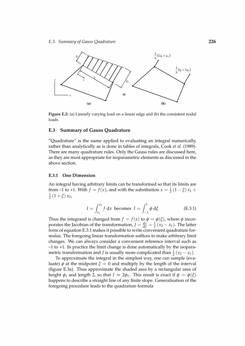
E.3. Summary of Gauss Quadrature 226
Ls
q1
q2
x
y
( )2126
qqL +
( )21 26
qqL +
=
(a) (b)
Figure E.2: (a) Linearly varying load on a linear edge and (b) the consistent nodalloads
E.3 Summary of Gauss Quadrature
”Quadrature” is the name applied to evaluating an integral numerically,rather than analytically as is done in tables of integrals, Cook et al. (1989).There are many quadrature rules. Only the Gauss rules are discussed here,as they are most appropriate for isoparametric elements as discussed in theabove section.
E.3.1 One Dimension
An integral having arbitrary limits can be transformed so that its limits arefrom –1 to +1. With f = f (x), and with the substitution x = 1
2 (1− ξ) x1 +12 (1 + ξ) x2,
I =∫ x2
x1
f dx becomes I =∫ 1
−1φ dξ (E.3.1)
Thus the integrand is changed from f = f (x) to φ = φ(ξ), where φ incor-porates the Jacobian of the transformation, J = dx
dξ = 12 (x2 − x1). The latter
form of equation E.3.1 makes it possible to write convenient quadrature for-mulas. The foregoing linear transformation suffices to make arbitrary limitchanges. We can always consider a convenient reference interval such as–1 to +1. In practice the limit change is done automatically by the isopara-metric transformation and J is usually more complicated than 1
2 (x2 − x1).To approximate the integral in the simplest way, one can sample (eva-
luate) φ at the midpoint ξ = 0 and multiply by the length of the interval(figure E.3a). Thus approximate the shaded area by a rectangular area ofheight φ1 and length 2, so that I ≈ 2φ1. This result is exact if φ = φ(ξ)happens to describe a straight line of any finite slope. Generalisation of theforegoing procedure leads to the quadrature formula

E.3. Summary of Gauss Quadrature 227
ξ-1 10
1
φ
φ1
φ=φ(ξ)
ξ-1 10
1
φ
φ1 φ2
2
ξ2ξ1
(a) (b)
Figure E.3: Gauss quadrature to compute the shaded area under the curveφ = φ(ξ), using (a) one and (b) two sampling points (Gauss points)
I =∫ 1
−1φ dξ ≈ W1φ1 + W2φ2 + · · ·+ Wnφn (E.3.2)
Thus, to approximate I, we must evaluate φ = φ(ξ) at each of the se-veral locations ξi to obtain ordinates φi, multiply each φi by an appropriateweight Wi, and add. In the one-point example, where I ≈ 2φ1, we haven = 1 and W1 = 2. Gauss was able to prescribe the locations ξi and weightsWi such that greatest accuracy is achieved for a given n. Sampling pointsare located symmetrically with respect to the center of the integration inter-val. Symmetrically paired points have the same weight Wi. Table E.1 givessample point locations and weights for a few cases.
These values are sometimes called Gauss-Legendre coefficients becausesampling point locations happen to be roots of Legendre polynomials. Itcan be shown that a polynomial of degree (2n− 1) is integrated exactly bya n-point Gauss quadrature. Use of more than n points will still producethe exact result. If the function is not a polynomial, Gauss quadrature isinexact, but becomes more accurate as more points are used.
E.3.2 Two Dimensions
Multidimensional Gauss rules, called Gaussian product rules, are formedby successive application of one-dimensional Gauss rules. In two dimensi-ons, consider the function φ = φ(ξ, η). Elect to integrate first with respect

E.3. Summary of Gauss Quadrature 228
Table E.1: Sampling points and weights for Gauss quadrature over the intervalξ = −1 to ξ = +1
Order n Location ξi of Sampling Point Weight Factor Wi
1 0 2
2 ±1 1√3
1
3 ±√
0.6 59
0 89
4 ±[
3+2√
1.27
] 12 1
2 −1
6√
1.2
±[
3−2√
1.27
] 12 1
2 + 16√
1.2
to ξ and then with respect to η.
I =∫ 1
−1
∫ 1
−1φ(ξ, η) dξdη ≈
∫ 1
−1
(n
∑i=1
Wiφ(ξi, η)
)dη
≈m
∑j=1
Wj
(n
∑i=1
Wiφ(ξi, ηj)
)=
m
∑j=1
n
∑i=1
WiWjφ(ξi, ηj)
(E.3.3)
Where m and n are the order of the Gauss rule in the ξ and η directions re-spectively. It is most common that the same rule is used in both directions,i.e. n = m. For the four-point rule depicted in figure E.4a, equation E.3.3becomes
I ≈ W1W1φ (ξ1, η1) + W1W2φ (ξ1, η2) + W2W1φ (ξ2, η1) + W2W2φ (ξ2, η2)= φ1 + φ3 + φ2 + φ4
(E.3.4)where φi is the numerical value of φ at the ith Gauss point. For the nine-point rule in figure E.4b, equation E.3.3 yields
I ≈ 2581 (φ1 + φ3 + φ7 + φ9) + 40
81 (φ2 + φ4 + φ6 + φ8) + 6481 φ5 (E.3.5)
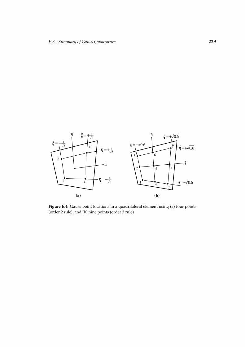
E.3. Summary of Gauss Quadrature 229
1
2
3
4
ξ
η
31−=ξ
31+=ξ
31+=η
31−=η
1
3
9
7
ξ
η
6.0−=ξ
6.0+=ξ
6.0+=η
6.0−=η
2 8
6
5
4
(a) (b)
Figure E.4: Gauss point locations in a quadrilateral element using (a) four points(order 2 rule), and (b) nine points (order 3 rule)

Appendix F
The Particle-in-Cell Method Based onthe Cosserat Continuum
F.1 Introduction
Problems in solid mechanics that involve history-dependent constitutiverelations are expressed more naturally in a Lagrangian computational frame.Similarly, a Lagrangian description is useful when following material freesurfaces or multiple materials. On the other hand, if large deformations areinvolved, a purely Lagrangian mesh can become tangled or require unre-asonably small time steps to be successful (Sulsky et al., 1995). For thesereasons the particle methods seem to be increasing in popularity.
The Particle-In-Cell (PIC) method uses two discretisations of the ma-terial, one based on a computational mesh and the other based on a col-lection of material points or “particles”. This approach combines the ad-vantages of Eulerian and Largrangian descriptions of the material whileavoiding the shortcomings of each. The equations of motion are solved ina Lagrangian frame on a computational grid, using standard finite elementmethods. Convection is modelled by moving the material points in thecomputed velocity field. Each material point carries its material propertieswithout error while it is moved. Since all the properties of the continuumare assigned to the numerical material points, the information carried bythese points is enough to characterise the flow and the grid carries no per-manent information. Thus, the grid can be discarded and reconstructed forcomputational convenience each time step.
To avoid confusion, x, y and z are used as indices for the three orthogo-nal coordinate directions. Numerical subscripts (1,2,3,4) are used to indi-cate element node numbers unless stated otherwise.
F.2 PIC Mass Representation
In the Lagrangian description of continuum mechanics, the material is di-vided into infinitesimal mass elements. Each mass element contains a fixedamount of mass for all the time. In PIC, these infinitesimal mass elementsare represented by a finite collection of Np material points or “particles”with fixed mass mp. Since mp is fixed, mass conservation, equation F.3.3, isautomatically satisfied.
Let the solid body under consideration initially occupy a region V(0) inR3 and V(t) for time t > 0. Let Xi be the initial position vector of a mate-
230

F.2. PIC Mass Representation 231
x1
x2
x1
x2p
iX
pix
0pV
pV
(a) (b)
FEM element
Subdomain
Figure F.1: Typical computational grid and material elements. (a) Initial configu-ration and (b) deformed configuration
rial point and xi the current position. Divide the initial configuration V(0)into Np subdomains, V0
p , with one material point (“particle”) identified atthe centroid of each V0
p . The coordinates of the particles at the centroid ofthe subdomains is denoted by Xp
i and the particle initially located at thecentroid of each subdomain will be tracked throughout the history of thematerial. Figure F.1 shows a typical rectangular FEM grid with 4-node ele-ments. Each FEM element is divided into four subdomains with a materialpoint at the centroid of each subdomain. The mass of a particle remainsconstant and is initially determined by
mp =∫
V0p
ρ0(Xp
i
)dV = ρV0
p (F.2.1)
where ρ0 is the initial mass density of the material and assumed constantthrough the material. The density represented by this collection of discretemass points will be approximated using a Dirac delta function
ρ0 (Xi) =Np
∑p=1
mpδ(Xi − Xp
i
)(F.2.2)
where the Dirac delta function is defined as
δ (x− a) =
0 x 6= a∞ x = a
and∫ +∞
−∞δ (x− a) dx = 1 (F.2.3)
Using this approximation, the total mass in the region is the same as thetotal mass given by the continuous density distribution ρ0 (Xi). Integration

F.2. PIC Mass Representation 232
over a subdomain gives
mp =∫
V0p
ρ0 (Xi) dV =∫
V0p
ρ0 (Xi) dV (F.2.4)
Now, consider a transformation to the current (deformed) configuration inwhich the same material points that were located at Xp
i at t = 0 are nowlocated at xp
i . Conservation of mass can be written as∫V0
p
ρ0 (Xi) dV =∫
Vp
ρ (xi, t) dV (F.2.5)
where ρ (xi, t) is the density and Vp is the current domain, figure F.1b. Inderiving an approximation for the density in the current configuration, werequire the approximation to satisfy conservation of mass which can alsobe written as ∫
V0p
ρ0 (Xi) dV =∫
Vp
ρ (xi, t) dV (F.2.6)
where ρ (xi, t) is the discrete approximation of the density in the currentconfiguration. Let J denote the Jacobian of the transformation from theinitial to the current configuration. Using Equations F.2.2 and F.2.4, andnoting that the Dirac delta function transforms as
δ(Xi − Xp
i
)=
δ(xi − xp
i
)J
(F.2.7)
we obtain ∫V0
p
ρ0 (Xi) dV =∫
V0p
ρ0 (Xi) dV
=∫
V0p
Np
∑p=1
mpδ(Xi − Xp
i
)dV
=∫
Vp
Np
∑p=1
mpδ(Xi − Xp
i
)J dV
=∫
Vp
Np
∑p=1
mpδ(xi − xp
i
)dV
(F.2.8)
Therefore, total mass is conserved if the density in the current configurationis given by the discrete approximation
ρ (xi, t) =Np
∑p=1
mpδ(xi − xp
i
)(F.2.9)

F.3. The Cosserat Governing Equations 233
F.3 The Cosserat Governing Equations
The linear momentum equation is given by equation C.2.11
ρdvi
dt= ρ fi + σij,j (F.3.1)
and the angular momentum (moment of momentum) by equation C.2.18
ε ijkσkj + µij,j + ρci = ρdhc
idt
(F.3.2)
The conservation of mass (continuity equation) is given by
dρ
dt+ ρvi,i = 0 (F.3.3)
F.4 The Weak Form of the Governing Equations
For the PIC computations (as for the finite element method) we require theweak form of the linear momentum and angular momentum balance equa-tions. The differential equations are said to state the problem in the strongform. An integral expression that implicitly contains the differential equati-ons is called the weak form, Cook et al. (1989). The strong form states conditi-ons that must be met at every material point, whereas the weak form statesconditions that must be met only in an average sense. The weak form isobtained in the usual way by multiplying equations F.3.1 and F.3.2 with thetest functions (vectors) wi and φi respectively.
σij,jwi + ρ fiwi − ρdvi
dtwi = 0 (F.4.1)
ε ijkσkjφi + µij,jφi + ρciφi − ρdhc
idt
φi = 0 (F.4.2)
Combining these equations and integrating over the domain V gives, (Pil-key and Wunderlich, 1994; Cook et al., 1989)
∫V
σij,jwi dV +∫
Vρ fiwi dV −
∫V
ρdvi
dtwi dV +
∫V
ε ijkσkjφi dV+∫V
µij,jφi dV +∫
Vρciφi dV −
∫V
ρdhc
idt
φi dV = 0
(F.4.3)

F.4. The Weak Form of the Governing Equations 234
Define the specific stress and specific couple stress respectively as
σsij =
σij
ρ→ σij = ρσs
ij and µsij =
µij
ρ→ µij = ρµs
ij (F.4.4)
where ρ is the material density. Assuming the material to be homogeneous,equation F.4.3 now becomes
∫V
ρσsij,jwi dV +
∫V
ρ fiwi dV −∫
Vρ
dvi
dtwi dV +
∫V
ρε ijkσskjφi dV+∫
Vρµs
ij,jφi dV +∫
Vρciφi dV −
∫V
ρdhc
idt
φi dV = 0
(F.4.5)
The first and fifth terms in equation F.4.5 can be expanded by using inte-gration by parts (Washizu, 1975)∫
Vρσs
ij,jwi dV =∫
Sρσs
ijnjwi dS−∫
Vρwi,jσ
sij dV
=∫
Sτiwi dS−
∫V
ρwi,jσsij dV
(F.4.6)
∫V
ρµsij,jφi dV =
∫S
ρµsijnjφi dS−
∫V
ρφi,jµsij dV
=∫
Smiφi dS−
∫V
ρφi,jµsij dV
(F.4.7)
where
τi = σijnj = ρσsijnj
= surface traction acting on surface with unit normal vector nj
mi = µijnj = ρµsijnj
= surface couple moment acting on surface with unit normal vector nj
This is an application of the divergence theorem of Gauss where S repres-ents a surface and nj the normal to the surface. Substitution of equation F.4.6and F.4.7 into equation F.4.5, collecting of terms and noting that ρε ijkσs
kjφi =ρεkjiσ
sijφk = −ρε ijkσs
ijφk, the governing equations can be written as
∫V
[ρσs
ij(wi,j + ε ijkφk
)+ ρφi,jµ
sij
]dV =∫
Vρ
[(fi −
dvi
dt
)wi +
(ci −
dhci
dt
)φi
]dV +
∫S(τiwi + miφi) dS
(F.4.8)

F.5. The Finite Element Representation 235
Equation F.4.8 must hold for all kinematically admissible wi and φi vanis-hing on those parts of the boundary where displacements and/or rotationsare prescribed. Substitution of the discrete density representation, equa-tion F.2.9 into equation F.4.8, yields a discrete expression where the inte-gration is performed as a sum of particle properties.
Nep
∑p=1
mp
[σ
spij
(wp
i,j + ε ijkφpk
)+ φ
pi,jµ
spij
]=
Nep
∑p=1
mp
[(f pi −
dvpi
dt
)wp
i +
(cp
i −dhcp
idt
)φ
pi
]+∫
S(τiwi + miφi) dS
(F.4.9)where the superscript p indicates that the value is evaluated at the particleposition and Nep is the number of particles in the finite element. Thus,equation F.4.9 is evaluated element-by-element.
F.5 The Finite Element Representation
Equation F.4.9 can be expanded into eight terms
©1Nep
∑p=1
mpvpi wp
i +©2Nep
∑p=1
mphcpi φ
pi = ©3
Nep
∑p=1
mpcpi φ
pi +©4
Nep
∑p=1
mp f pi wp
i −
©5Nep
∑p=1
mpσspij wp
i,j −©6Nep
∑p=1
mpσspij ε ijkφ
pk−
©7Nep
∑p=1
mpφpi,jµ
spij +©8
∫S(τiwi + miφi) dS
(F.5.1)
For the two-dimensional case, the terms are written in matrix notation:
©1Nep
∑p=1
mpvpi wp
i =Nep
∑p=1
mp[wp
x wpy wp
z] vp
xvp
y0
(F.5.2)
where the velocity vpz = 0.
©2Nep
∑p=1
mphcpi φ
pi =
Nep
∑p=1
mp[φ
px φ
py φ
pz] 0
0hcp
z
(F.5.3)

F.5. The Finite Element Representation 236
where the rate of angular momentum hcpx = hcp
y = 0
©3Nep
∑p=1
mpcpi φ
pi =
Nep
∑p=
mp[φ
px φ
py φ
pz] 0
0cp
z
(F.5.4)
where the body couples cpx = cp
y = 0
©4Nep
∑p=1
mp f pi wp
i =Nep
∑p=
mp[wp
x wpy wp
z] f p
xf py0
(F.5.5)
where the body force f pz = 0
©5Nep
∑p=1
mpσspij wp
i,j =Nep
∑p=1
mp[wp
x,x wpy,y wp
x,y wpy,x]
σspxx
σspyy
σspxy
σspyx
(F.5.6)
where only the stresses applicable to the two-dimensional case have beenincluded.
©6Nep
∑p=1
mpσspij ε ijkφ
pk =
Nep
∑p=1
mp[0 0 φ
pz − φ
pz]
σspxx
σspyy
σspxy
σspyx
(F.5.7)
©7Nep
∑p=1
mpφpi,jµ
spij =
Nep
∑p=1
mp[φ
pz,xφ
pz,y] [µ
spzx
µspzy
](F.5.8)
where the other couple stresses are zero.
©8
∫S(τiwi + miφi) dS =
∫S
[wx wy wz] τx
τy0
+[φx φy φz
] 00
mz
dS
=∫
S
[wx wy φz
] τxτymz
dS
(F.5.9)where the surface traction τz = 0 and the surface couples mx = my = 0. Inthe last equation the two sums have been added by simply discarding allzero products.

F.5. The Finite Element Representation 237
Using four node isoparametric finite elements, the test functions wi andφi can be written in terms of the nodal values and shape functions, for ex-ample
wx = [wx1 wx2 wx3 wx4]
N1N2N3N4
(F.5.10)
where wx1 is the scalar value of the test vector in the x-direction at node 1of the element and the shape function is given by
Ni =[ 1
4 (1− ξ) (1− η) ; 14 (1 + ξ) (1− η) ; 1
4 (1 + ξ) (1 + η) ; 14 (1− ξ) (1 + η)
](F.5.11)
The derivatives with respect to x and y can be written as
wx,x = [wx1 wx2 wx3 wx4]
N1,xN2,xN3,xN4,x
(F.5.12)
which can be combined with the test function φi and the other derivativesinto a matrix expression
wx,xwy,ywx,ywy,xφz,xφz,y
=
N1,x 0 0 N2,x 0 0 N3,x 0 0 N4,x 0 00 N1,y 0 0 N2,y 0 0 N3,y 0 0 N4,y 0
N1,y 0 0 N2,y 0 0 N3,y 0 0 N4,y 0 00 N1,x 0 0 N2,x 0 0 N3,x 0 0 N4,x 00 0 N1,x 0 0 N2,x 0 0 N3,x 0 0 N4,x0 0 N1,y 0 0 N2,y 0 0 N3,y 0 0 N4,y
wx1wy1φz1wx2wy2φz2wx3wy3φz3wx4wy4φz4
(F.5.13)

F.5. The Finite Element Representation 238
Similarly, the derivatives with respect to element coordinates can be writtenas
wx,ξwy,ηwx,ηwy,ξφz,ξφz,η
=
N1,ξ 0 0 N2,ξ 0 0 N3,ξ 0 0 N4,ξ 0 00 N1,η 0 0 N2,η 0 0 N3,η 0 0 N4,η 0
N1,η 0 0 N2,η 0 0 N3,η 0 0 N4,η 0 00 N1,ξ 0 0 N2,ξ 0 0 N3,ξ 0 0 N4,ξ 00 0 N1,ξ 0 0 N2,ξ 0 0 N3,ξ 0 0 N4,ξ0 0 N1,η 0 0 N2,η 0 0 N3,η 0 0 N4,η
wx1wy1φz1wx2wy2φz2wx3wy3φz3wx4wy4φz4
(F.5.14)
In some of the terms in equation F.5.1, the vector[wx,x wy,y wx,y wy,x φz,x φz,y
]is needed, but cannot be obtained from expression F.5.13, since the partialderivatives of Ni with respect to x and y are not available. It is however pos-sible to obtain the vector
[wx,ξ wy,η wx,η wy,ξ φz,ξ φz,η
]from equation F.5.14
since the derivatives Ni with respect to ξ and η can easily be calculatedusing equation F.5.11.
Seek an expression for Γ such that
wx,xwy,ywx,ywy,xφz,xφz,y
= Γ
wx,ξwy,ηwx,ηwy,ξφz,ξφz,η
(F.5.15)
By the chain rule, for example
∂wx
∂x=
∂wx
∂ξ
∂ξ
∂x+
∂wx
∂η
∂η
∂x∂wx
∂y=
∂wx
∂ξ
∂ξ
∂y+
∂wx
∂η
∂η
∂y
(F.5.16)

F.5. The Finite Element Representation 239
Unfortunately, the partial derivatives of ξ and η with respect to x and y arenot available from the above equations. Therefore, write the inverse first,which is easily done.
∂wx
∂ξ=
∂wx
∂x∂x∂ξ
+∂wx
∂y∂y∂ξ
∂wx
∂η=
∂wx
∂x∂x∂η
+∂wx
∂y∂y∂η
(F.5.17)
Writing equation F.5.17 in matrix notation[wx,ξwx,η
]= J
[wx,xwx,y
]=[
x,ξ y,ξx,η y,η
] [wx,xwx,y
](F.5.18)
where J is called the Jacobian matrix. Using the definition of the coordina-tes (x, y) within an element with respect to the element nodal coordinates(xi, yi).
x =4
∑i=1
Nixi y =4
∑i=1
Niyi (F.5.19)
the Jacobian can be written as
J =[
x,ξ y,ξx,η y,η
]=[
∑4i=1 Ni,ξ xi ∑4
i=1 Ni,ξyi
∑4i=1 Ni,ηxi ∑4
i=1 Ni,ηyi
]=[
J11 J12J21 J22
] (F.5.20)
Applying a similar procedure to the other variables, it follows
wx,ξwy,ηwx,ηwy,ξφz,ξφz,η
= J
wx,xwy,ywx,ywy,xφz,xφz,y
=
x,ξ 0 y,ξ 0 0 00 y,η 0 x,η 0 0
x,η 0 y,η 0 0 00 y,ξ 0 x,ξ 0 00 0 0 0 x,ξ y,ξ0 0 0 0 x,η y,η
wx,xwy,ywx,ywy,xφz,xφz,y
=
J11 0 J12 0 0 00 J22 0 J21 0 0
J21 0 J22 0 0 00 J12 0 J11 0 00 0 0 0 J11 J120 0 0 0 J21 J22
wx,xwy,ywx,ywy,xφz,xφz,y
(F.5.21)

F.5. The Finite Element Representation 240
By comparing equation F.5.15 with equation F.5.18, it can be seen that Γ isthe inverse of J
Γ = J−1 =1|J|
[J22 −J12−J21 J11
](F.5.22)
where |J| is the determinant of the Jacobian matrix. Applying this to equa-tion F.5.21 yields
wx,xwy,ywx,ywy,xφz,xφz,y
= Γ
wx,ξwy,ηwx,ηwy,ξφz,ξφz,η
=1J
J22 0 −J12 0 0 00 J11 0 −J21 0 0−J21 0 J11 0 0 0
0 −J12 0 J22 0 00 0 0 0 J22 −J120 0 0 0 −J21 J11
wx,ξwy,ηwx,ηwy,ξφz,ξφz,η
(F.5.23)
where J = J11 J22 − J21 J12 is the determinant of J. Taking the transpose
[wx,x wy,y wx,y wy,x φz,x φz,y
]=
1J[wx,ξ wy,η wx,η wy,ξ φz,ξ φz,η
]
J22 0 −J21 0 0 00 J11 0 −J12 0 0−J12 0 J11 0 0 0
0 −J21 0 J22 0 00 0 0 0 J22 −J210 0 0 0 −J12 J11
(F.5.24)
and from equation F.5.14

F.5. The Finite Element Representation 241
[wx,ξ wy,η wx,η wy,ξ φz,ξ φz,η
]=[
wx1 wy1 φz1 wx2 wy2 φz2 wx3 wy3 φz3 wx4 wy4 φz4]·
N1,ξ 0 N1,η 0 0 00 N1,η 0 N1,ξ 0 00 0 0 0 N1,ξ N1,η
N2,ξ 0 N2,η 0 0 00 N2,η 0 N2,ξ 0 00 0 0 0 N2,ξ N2,η
N3,ξ 0 N3,η 0 0 00 N3,η 0 N3,ξ 0 00 0 0 0 N3,ξ N3,η
N4,ξ 0 N4,η 0 0 00 N4,η 0 N4,ξ 0 00 0 0 0 N4,ξ N4,η
(F.5.25)
Thus, equation F.5.24 becomes
[wx,x wy,y wx,y wy,x φz,x φz,y
]=
1J[wx1 wy1 φz1 wx2 wy2 φz2 wx3 wy3 φz3 wx4 wy4 φz4
]·
N1,ξ 0 N1,η 0 0 00 N1,η 0 N1,ξ 0 00 0 0 0 N1,ξ N1,η
N2,ξ 0 N2,η 0 0 00 N2,η 0 N2,ξ 0 00 0 0 0 N2,ξ N2,η
N3,ξ 0 N3,η 0 0 00 N3,η 0 N3,ξ 0 00 0 0 0 N3,ξ N3,η
N4,ξ 0 N4,η 0 0 00 N4,η 0 N4,ξ 0 00 0 0 0 N4,ξ N4,η
·
J22 0 −J21 0 0 00 J11 0 −J12 0 0−J12 0 J11 0 0 0
0 −J21 0 J22 0 00 0 0 0 J22 −J210 0 0 0 −J12 J11
(F.5.26)
Equation F.5.26 can now be substituted into terms 5 and 7 of equation F.5.1.
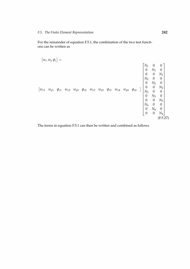
F.5. The Finite Element Representation 242
For the remainder of equation F.5.1, the combination of the two test functi-ons can be written as
[wx wy φz
]=
[wx1 wy1 φz1 wx2 wy2 φz2 wx3 wy3 φz3 wx4 wy4 φz4
]
N1 0 00 N1 00 0 N1
N2 0 00 N2 00 0 N2
N3 0 00 N3 00 0 N3
N4 0 00 N4 00 0 N4
(F.5.27)
The terms in equation F.5.1 can then be written and combined as follows.

F.5. The Finite Element Representation 243
©1 +©2 :
Nep
∑p=1
mp(vp
i wpi + hcp
i φpi)
=Nep
∑p=1
mp[wp
x wpy φ
pz] vp
xvp
yhcp
z
=
Nep
∑p=1
mp[wx1 wy1 φz1 wx2 wy2 φz2 wx3 wy3 φz3 wx4 wy4 φz4
]·
N1 0 00 N1 00 0 N1
N2 0 00 N2 00 0 N2
N3 0 00 N3 00 0 N3
N4 0 00 N4 00 0 N4
p
·
N1 0 0 N2 0 0 N3 0 N4 0 00 N1 0 0 N2 0 0 N3 0 N4 00 0 N1 0 0 N2 0 0 N3 0 N4
p
vx1vy1hc
z1vx2vy2hc
z2vx3vy3hc
z3vx4vy4hc
z4
=
Nep
∑p=1
mp[wx1 wy1 φz1 wx2 wy2 φz2 wx3 wy3 φz3 wx4 wy4 φz4
]·
N21 0 0 N2 N1 0 0 N3 N1 0 0 N4 N1 0 0
0 N21 0 0 N2 N1 0 0 N3 N1 0 0 N4 N1 0
0 0 N21 0 0 N2 N1 0 0 N3 N1 0 0 N4 N1
N1 N2 0 0 N22 0 0 N3 N2 0 0 N4 N2 0 0
0 N1 N2 0 0 N22 0 0 N3 N2 0 0 N4 N2 0
0 0 N1 N2 0 0 N22 0 0 N3 N2 0 0 N4 N2
N1 N3 0 0 N2 N3 0 0 N23 0 0 N4 N3 0 0
0 N1 N3 0 0 N2 N3 0 0 N23 0 0 N4 N3 0
0 0 N1 N3 0 0 N2 N3 0 0 N23 0 0 N4 N3
N1 N4 0 0 N2 N4 0 0 N3 N4 0 0 N24 0 0
0 N1 N4 0 0 N2 N4 0 0 N3 N4 0 0 N24 0
0 0 N1 N4 0 0 N2 N4 0 0 N3 N4 0 0 N24
p
·
vx1vy1hc
z1vx2vy2hc
z2vx3vy3hc
z3vx4vy4hc
z4
(F.5.28)

F.5. The Finite Element Representation 244
©3 +©4 :
Nep
∑p=1
mp[wp
x wpy φ
pz] f p
xf py
cpz
=
Nep
∑p=1
mp[wx1 wy1 φz1 wx2 wy2 φz2 wx3 wy3 φz3 wx4 wy4 φz4
]·
N1 0 00 N1 00 0 N1
N2 0 00 N2 00 0 N2
N3 0 00 N3 00 0 N3
N4 0 00 N4 00 0 N4
p
f px
f py
cpz
(F.5.29)
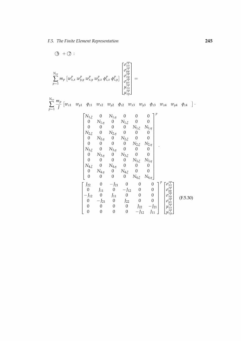
F.5. The Finite Element Representation 245
©5 +©7 :
Nep
∑p=1
mp[wp
x,x wpy,y wp
x,y wpy,x φ
pz,x φ
pz,y]
σspxx
σspyy
σspxy
σspyx
µspzx
µspzy
=
Nep
∑p=1
mp
J[wx1 wy1 φz1 wx2 wy2 φz2 wx3 wy3 φz3 wx4 wy4 φz4
]·
N1,ξ 0 N1,η 0 0 00 N1,η 0 N1,ξ 0 00 0 0 0 N1,ξ N1,η
N2,ξ 0 N2,η 0 0 00 N2,η 0 N2,ξ 0 00 0 0 0 N2,ξ N2,η
N3,ξ 0 N3,η 0 0 00 N3,η 0 N3,ξ 0 00 0 0 0 N3,ξ N3,η
N4,ξ 0 N4,η 0 0 00 N4,η 0 N4,ξ 0 00 0 0 0 N4,ξ N4,η
p
·
J22 0 −J21 0 0 00 J11 0 −J12 0 0−J12 0 J11 0 0 0
0 −J21 0 J22 0 00 0 0 0 J22 −J210 0 0 0 −J12 J11
p
σspxx
σspyy
σspxy
σspyx
µspzx
µspzy
(F.5.30)

F.5. The Finite Element Representation 246
©6 :
Nep
∑p=1
mp[0 0 φ
pz −φ
pz 0 0
]
σspxx
σspyy
σspxy
σspyx
µspzx
µspzy
=
Nep
∑p=1
mp[wx1 wy1 φz1 wx2 wy2 φz2 wx3 wy3 φz3 wx4 wy4 φz4
]·
0 0 0 0 0 00 0 0 0 0 00 0 N1 −N1 0 00 0 0 0 0 00 0 0 0 0 00 0 N2 −N2 0 00 0 0 0 0 00 0 0 0 0 00 0 N3 −N3 0 00 0 0 0 0 00 0 0 0 0 00 0 N4 −N4 0 0
p
σspxx
σspyy
σspxy
σspyx
µspzx
µspzy
(F.5.31)
where the stresses have been assembled in a matrix similar to that in equa-tion F.5.30.
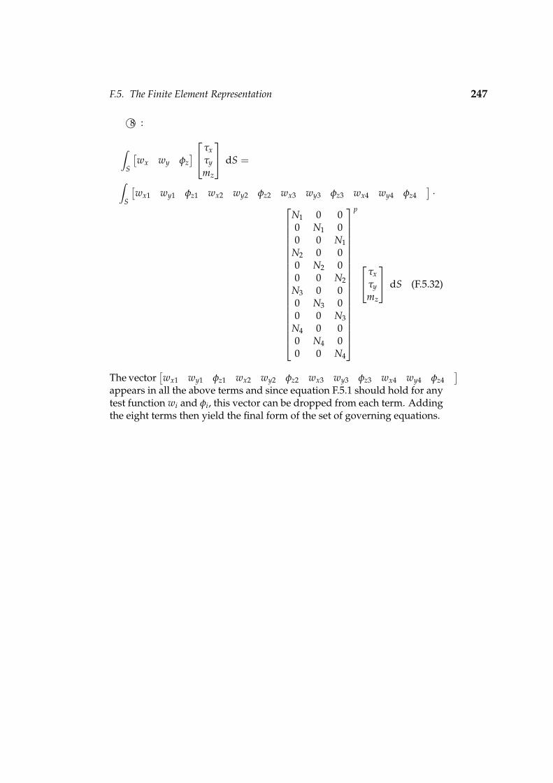
F.5. The Finite Element Representation 247
©8 :
∫S
[wx wy φz
] τxτymz
dS =
∫S
[wx1 wy1 φz1 wx2 wy2 φz2 wx3 wy3 φz3 wx4 wy4 φz4
]·
N1 0 00 N1 00 0 N1
N2 0 00 N2 00 0 N2
N3 0 00 N3 00 0 N3
N4 0 00 N4 00 0 N4
p
τxτymz
dS (F.5.32)
The vector[wx1 wy1 φz1 wx2 wy2 φz2 wx3 wy3 φz3 wx4 wy4 φz4
]appears in all the above terms and since equation F.5.1 should hold for anytest function wi and φi, this vector can be dropped from each term. Addingthe eight terms then yield the final form of the set of governing equations.

F.5. The Finite Element Representation 248
Nep
∑p=1
mp
N21 0 0 N2 N1 0 0 N3 N1 0 0 N4 N1 0 0
0 N21 0 0 N2 N1 0 0 N3 N1 0 0 N4 N1 0
0 0 N21 0 0 N2 N1 0 0 N3 N1 0 0 N4 N1
N1 N2 0 0 N22 0 0 N3 N2 0 0 N4 N2 0 0
0 N1 N2 0 0 N22 0 0 N3 N2 0 0 N4 N2 0
0 0 N1 N2 0 0 N22 0 0 N3 N2 0 0 N4 N2
N1 N3 0 0 N2 N3 0 0 N23 0 0 N4 N3 0 0
0 N1 N3 0 0 N2 N3 0 0 N23 0 0 N4 N3 0
0 0 N1 N3 0 0 N2 N3 0 0 N23 0 0 N4 N3
N1 N4 0 0 N2 N4 0 0 N3 N4 0 0 N24 0 0
0 N1 N4 0 0 N2 N4 0 0 N3 N4 0 0 N24 0
0 0 N1 N4 0 0 N2 N4 0 0 N3 N4 0 0 N24
p
·
vx1vy1hc
z1vx2vy2hc
z2vx3vy3hc
z3vx4vy4hc
z4
=Nep
∑p=1
mp
N1 0 00 N1 00 0 N1
N2 0 00 N2 00 0 N2
N3 0 00 N3 00 0 N3
N4 0 00 N4 00 0 N4
p
f px
f py
cpz
−
Nep
∑p=1
mp
J
N1,ξ 0 N1,η 0 0 00 N1,η 0 N1,ξ 0 00 0 0 0 N1,ξ N1,η
N2,ξ 0 N2,η 0 0 00 N2,η 0 N2,ξ 0 00 0 0 0 N2,ξ N2,η
N3,ξ 0 N3,η 0 0 00 N3,η 0 N3,ξ 0 00 0 0 0 N3,ξ N3,η
N4,ξ 0 N4,η 0 0 00 N4,η 0 N4,ξ 0 00 0 0 0 N4,ξ N4,η
p
·
J22 0 −J21 0 0 00 J11 0 −J12 0 0
−J12 0 J11 0 0 00 −J21 0 J22 0 00 0 0 0 J22 −J210 0 0 0 −J12 J11
p
σspxx
σspyy
σspxy
σspyx
µspzx
µspzy
−
Nep
∑p=1
mp
0 0 0 0 0 00 0 0 0 0 00 0 N1 −N1 0 00 0 0 0 0 00 0 0 0 0 00 0 N2 −N2 0 00 0 0 0 0 00 0 0 0 0 00 0 N3 −N3 0 00 0 0 0 0 00 0 0 0 0 00 0 N4 −N4 0 0
p
σspxx
σspyy
σspxy
σspyx
µspzx
µspzy
+∫
S
N1 0 00 N1 00 0 N1
N2 0 00 N2 00 0 N2
N3 0 00 N3 00 0 N3
N4 0 00 N4 00 0 N4
p
τxτymz
dS (F.5.33)
Equation F.5.33 is applicable to a single element since the sum runs over all
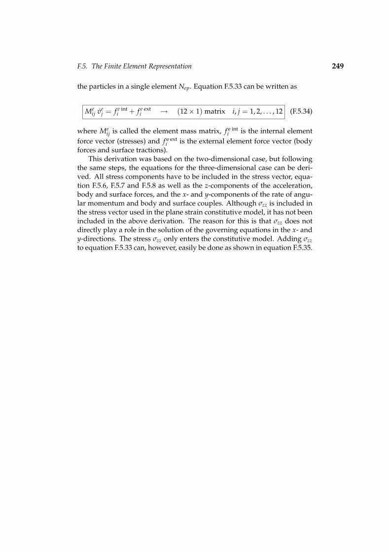
F.5. The Finite Element Representation 249
the particles in a single element Nep. Equation F.5.33 can be written as
Meij ve
j = f e inti + f e ext
i → (12× 1) matrix i, j = 1, 2, . . . , 12 (F.5.34)
where Meij is called the element mass matrix, f e int
i is the internal elementforce vector (stresses) and f e ext
i is the external element force vector (bodyforces and surface tractions).
This derivation was based on the two-dimensional case, but followingthe same steps, the equations for the three-dimensional case can be deri-ved. All stress components have to be included in the stress vector, equa-tion F.5.6, F.5.7 and F.5.8 as well as the z-components of the acceleration,body and surface forces, and the x- and y-components of the rate of angu-lar momentum and body and surface couples. Although σzz is included inthe stress vector used in the plane strain constitutive model, it has not beenincluded in the above derivation. The reason for this is that σzz does notdirectly play a role in the solution of the governing equations in the x- andy-directions. The stress σzz only enters the constitutive model. Adding σzzto equation F.5.33 can, however, easily be done as shown in equation F.5.35.

F.5. The Finite Element Representation 250
Nep
∑p=1
mp
N21 0 0 N2 N1 0 0 N3 N1 0 0 N4 N1 0 0
0 N21 0 0 N2 N1 0 0 N3 N1 0 0 N4 N1 0
0 0 N21 0 0 N2 N1 0 0 N3 N1 0 0 N4 N1
N1 N2 0 0 N22 0 0 N3 N2 0 0 N4 N2 0 0
0 N1 N2 0 0 N22 0 0 N3 N2 0 0 N4 N2 0
0 0 N1 N2 0 0 N22 0 0 N3 N2 0 0 N4 N2
N1 N3 0 0 N2 N3 0 0 N23 0 0 N4 N3 0 0
0 N1 N3 0 0 N2 N3 0 0 N23 0 0 N4 N3 0
0 0 N1 N3 0 0 N2 N3 0 0 N23 0 0 N4 N3
N1 N4 0 0 N2 N4 0 0 N3 N4 0 0 N24 0 0
0 N1 N4 0 0 N2 N4 0 0 N3 N4 0 0 N24 0
0 0 N1 N4 0 0 N2 N4 0 0 N3 N4 0 0 N24
p
·
vx1vy1hc
z1vx2vy2hc
z2vx3vy3hc
z3vx4vy4hc
z4
=Nep
∑p=1
mp
N1 0 00 N1 00 0 N1
N2 0 00 N2 00 0 N2
N3 0 00 N3 00 0 N3
N4 0 00 N4 00 0 N4
p
f px
f py
cpz
−
Nep
∑p=1
mp
J
N1,ξ 0 0 N1,η 0 0 00 N1,η 0 0 N1,ξ 0 00 0 0 0 0 N1,ξ N1,η
N2,ξ 0 0 N2,η 0 0 00 N2,η 0 0 N2,ξ 0 00 0 0 0 0 N2,ξ N2,η
N3,ξ 0 0 N3,η 0 0 00 N3,η 0 0 N3,ξ 0 00 0 0 0 0 N3,ξ N3,η
N4,ξ 0 0 N4,η 0 0 00 N4,η 0 0 N4,ξ 0 00 0 0 0 0 N4,ξ N4,η
p
·
J22 0 0 −J21 0 0 00 J11 0 0 −J12 0 0
−J12 0 0 J11 0 0 00 −J21 0 0 J22 0 00 0 0 0 0 J22 −J210 0 0 0 0 −J12 J11
p
σspxx
σspyy
σspzz
σspxy
σspyx
µspzx
µspzy
−
Nep
∑p=1
mp
0 0 0 0 0 0 00 0 0 0 0 0 00 0 0 N1 −N1 0 00 0 0 0 0 0 00 0 0 0 0 0 00 0 0 N2 −N2 0 00 0 0 0 0 0 00 0 0 0 0 0 00 0 0 N3 −N3 0 00 0 0 0 0 0 00 0 0 0 0 0 00 0 0 N4 −N4 0 0
p
σspxx
σspyy
σspzz
σspxy
σspyx
µspzx
µspzy
+∫
S
N1 0 00 N1 00 0 N1
N2 0 00 N2 00 0 N2
N3 0 00 N3 00 0 N3
N4 0 00 N4 00 0 N4
p
τxτymz
dS (F.5.35)

F.6. Numerical Algorithm 251
F.6 Numerical Algorithm
Equation F.5.35 is derived for a single finite element. The system is sol-ved by sweeping through all the elements, calculating all the known terms(right hand side) in equation F.5.35 and assembling it into system arrays.
Ne
∑e=1
Meijv
ej = f e int
i + f e exti i, j = 1, 2, . . . , 12 (F.6.1)
where Ne is the number of elements. Summing over all the elements yields
Mijvj = f inti + f ext
i i, j = 1, 2, . . . , Ndo f (F.6.2)
where Ndo f is the number of degrees-of-freedom. Equation F.6.2 has a formsimilar to that obtained by traditional finite element schemes, however, themass matrix Mij (assembled from element mass matrices, Me
ij) varies withtime and therefore must be computed each time step. Since the particlesmove through the mesh, the entries in the mass matrix can vary when par-ticles move within the elements, but it can also change from size as partic-les move from one element to another. In other words, the total numberof degrees-of-freedom in the system can vary. The following steps describethe numerical algorithm.
F.6.1 Initialisation Phase
In this phase, information is transferred from the particles to the grid. Inorder to solve the discrete governing equation, information must be gathe-red from the particles for the initialisation phase. The mass matrix mustbe formed, the internal forces accumulated at the nodes using the specificstresses at the particles and the gradient of the shape functions.
Begin by assuming that for each particle its position vector, velocity vec-tor, accumulated strain components, accumulated stress components andhistory dependent variables are known. Linked lists are used to keep trackof particles, elements and entities. An entity is defined as an object whichmay have specific properties and/or constitutive models.
Figure F.2 shows the relation between particles, elements and entities.The initial number (usually 4 or 9) and positions of particles within a sin-gle element are specified. To generate an entity, its boundary is specifiedand particles, with the properties of the specific entity, are generated at thespecified element positions which are within the entity boundary. Theseparticles will always belong to this entity, since they define the entity. Eachelement has a list containing particle addresses to all the particles withinthe element. Each entity has a list containing addresses to all the elementsthat contain one or more of its particles. For example, in figure F.2, entityA will have in its element list: element 1, 2, 3, 9, 10, 11, 17, 18, 19, 26 and

F.6. Numerical Algorithm 252
Entity A Entity B
1 2 3
9 10 11
17 18 19
26 27
23
4 5
Figure F.2: Relation between particles, elements and entities
27. Element 2 will have in its particle list: particle 3, 4 and 5. In the initiali-sation phase, these lists are updated and used to calculate the mass matrixand force vectors.
Since there are generally more particles than grid points (nodes), a weigh-ted least squares approach is used to determine nodal velocities from thevelocities at the particles to initialise each time step. The weighting is themass of the particle. The result is the following equation which must besolved for the nodal velocities vj at time t, i.e. vt
j.
Ne
∑e=1
Me,tij ve,t
j =Ne
∑e=1
Nep
∑p=1
mp
N1 0 00 N1 00 0 N1
N2 0 00 N2 00 0 N2
N3 0 00 N3 00 0 N3
N4 0 00 N4 00 0 N4
p,t
vp,tx
vp,ty
hcp,tz
Ne
∑e=1
Me,tij ve,t
j = v′e,ti i, j = 1, 2, . . . , 12
(F.6.3)

F.6. Numerical Algorithm 253
where vpx and vp
y are the particle x- and y-velocity components and hcpz is
the particle angular momentum and all the variables are evaluated at timet as indicated by the superscript.
The vector vej is given by
[vx1 vy1 hc
z1 vx2 vy2 hcz2 vx3 vy3 hc
z3 vx4 vy4 hcz4
]T.Summing over all the elements yields
Mtijv
tj = v
′ti i, j = 1, 2, . . . , Ndo f (F.6.4)
F.6.2 Lagrangian Phase
During the Lagrangian phase of the computation, the discrete governingequation, equation F.6.2, is solved for the nodal accelerations at time t. Thesolution in a Lagrangian frame means that the nonlinear convective termsthat are troublesome in purely Eulerian calculations do not appear in theformulation (Sulsky et al., 1995). With the nodal accelerations computed,the nodal velocities can be updated with the use of an explicit time integra-tor.
vt+1i = vt
i + ∆tvti i, j = 1, 2, . . . , 12 (F.6.5)
where ∆t is the current time increment. During this phase of the computa-tion, the nodes are assumed to move according to this computed velocity.The updates of particle velocity and position are consistent with the isopa-rametric approach
xp,t+1i = xp,t
i +
∆t
N1 0 0 N2 0 0 N3 0 N4 0 00 N1 0 0 N2 0 0 N3 0 N4 00 0 N1 0 0 N2 0 0 N3 0 N4
p,t
vx1vy1hc
z1vx2vy2hc
z2vx3vy3hc
z3vx4vy4hc
z4
t+1
(F.6.6)
or in index notation
xp,t+1i = xp,t
i + ∆t Np,tij ve,t+1
j (F.6.7)

F.6. Numerical Algorithm 254
The position vector is given by xpi =
[xp yp Jp
zzwcpz], where wc
z is the Cos-serat rotation, equation C.3.4, and should not be confused with the testfunction wi. The vector ve,t+1
j is the nodal velocities of the element contai-
ning the particle. This vector is extracted from the system solution vt+1i in
equation F.6.5. A similar equation can be written for the velocity update.
vp,t+1i = vp,t
i +
∆t
N1 0 0 N2 0 0 N3 0 N4 0 00 N1 0 0 N2 0 0 N3 0 N4 00 0 N1 0 0 N2 0 0 N3 0 N4
p,t
vx1vy1hc
z1vx2vy2hc
z2vx3vy3hc
z3vx4vy4hc
z4
t
(F.6.8)
or in index notation
vp,t+1i = vp,t
i + ∆t Np,tij ve,t
j (F.6.9)
where ve,tj is the nodal acceleration of the element containing the particle.
This vector is extracted from the system solution vti obtained from solving
equation F.6.2.During the Lagrangian step, each element is assumed to deform in the
flow of material so that points in the interior of the element move in pro-portion to the motion of the nodes, as given by the representation using thenodal shape (basis) functions. Since shape functions are used to map thenodal velocity continuously to the interior of the element, the positions ofthe particles are updated by moving them in a single-valued, continuousvelocity field. Similarly, the velocity of a material is updated by mappingthe nodal accelerations to the particle position. Because the velocity field issingle-valued, interpenetration of material is precluded. This feature of thealgorithm allows simulations of impact and penetration without the needfor a special contact algorithm (Sulsky et al., 1995).
For history dependent materials, it has been convenient to carry strainand stress, as well as history variables along with the material points. Ap-plying constitutive equations at material points (particles) allows easy eva-luation and tracking of history dependent variables. It also allows compu-tations with multiple materials to be performed easily since each particle

F.6. Numerical Algorithm 255
retains its identity (material or entity properties) throughout the computa-tion. Another difference between equation F.6.2 and traditional finite ele-ment formulations is that the particles, where constitutive equations areapplied, move from one element to another rather than remain at the cen-tre or Gauss points of an element.
To describe the stress computations in its simplest form, strain incre-ments are obtained from gradients of the nodal velocities evaluated at theparticle positions. Then, given a strain increment at the particle, along withcurrent values of history variables and material parameters, standard rou-tines are used to evaluate the stress increment and update history variables.The internal forces at the nodes are then calculated directly from the stressat the particles for the next time step.
The single, tensorial deformation measure is given by, equation C.3.7
λij = ui,j + ε ijkwck (F.6.10)
or for planar deformation
λij =
λxx λxy λxzλyx λyy λyzλzx λzy λzz
=
ux,x(ux,y + wc
z)
0(uy,x − wc
z)
uy,y 00 0 uz,z
The micro-curvature is given by
κij = wci,j (F.6.11)
or for planar deformation
κij =
0 0 00 0 0
κzx κzy 0
In formulating elasto-plasticity, it is useful to rather use generalised curva-tures κzxl and κzyl, where l is a material parameter with the dimension oflength. It is this parameter which effectively sets the internal length scalein the continuum, and therefore has the role of a “characteristic length”.
The strain components can be assembled in a vector (for the two-dimensionalcase)
εci =
[λxx λyy λzz λxy λyx κzxl κzyl
](F.6.12)
Note that the normal strain in the z-direction, λzz = uz,z, has also been in-cluded in the strain vector. This has been done because, although this straincomponent remains zero under plane strain conditions during the entireloading process, this is not necessarily the case for the elastic and plasticcontributions of this strain component. Also note that by multiplying the

F.6. Numerical Algorithm 256
micro-curvatures by the length parameter l, all components of the strainvector εc
i have the same dimension. The strain rate vector can be written as
εci =
[vx,x vy,y vz,z
(vx,y + wc
z) (
vy,x − wcz)
wcz,xl wc
z,yl]
(F.6.13)
Making use of equation F.5.26, the terms in equation F.6.13 can be compu-ted at the particle positions.
[vp
x,x vpy,y vp
x,y vpy,x wcp
z,x wcpz,y]
=1J[vx1 vy1 wc
z1 vx2 vy2 wcz2 vx3 vy3 wc
z3 vx4 vy4 wcz4
]·
N1,ξ 0 N1,η 0 0 00 N1,η 0 N1,ξ 0 00 0 0 0 N1,ξ N1,η
N2,ξ 0 N2,η 0 0 00 N2,η 0 N2,ξ 0 00 0 0 0 N2,ξ N2,η
N3,ξ 0 N3,η 0 0 00 N3,η 0 N3,ξ 0 00 0 0 0 N3,ξ N3,η
N4,ξ 0 N4,η 0 0 00 N4,η 0 N4,ξ 0 00 0 0 0 N4,ξ N4,η
p
·
J22 0 −J21 0 0 00 J11 0 −J12 0 0−J12 0 J11 0 0 0
0 −J21 0 J22 0 00 0 0 0 J22 −J210 0 0 0 −J12 J11
p
(F.6.14)
and vpz,z = 0. Further, hc
z[m2·s−1] = Jzz
[m2] wc
z[s−1], equation D.3.10, i.e.
wcz = hc
zJzz
. Equation F.6.14 becomes
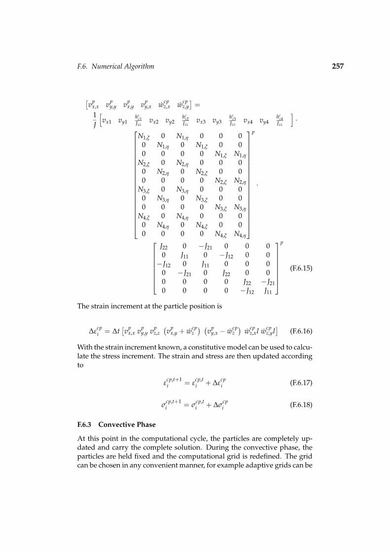
F.6. Numerical Algorithm 257
[vp
x,x vpy,y vp
x,y vpy,x wcp
z,x wcpz,y]
=1J
[vx1 vy1
hcz1
Jzzvx2 vy2
hcz2
Jzzvx3 vy3
hcz3
Jzzvx4 vy4
hcz4
Jzz
]·
N1,ξ 0 N1,η 0 0 00 N1,η 0 N1,ξ 0 00 0 0 0 N1,ξ N1,η
N2,ξ 0 N2,η 0 0 00 N2,η 0 N2,ξ 0 00 0 0 0 N2,ξ N2,η
N3,ξ 0 N3,η 0 0 00 N3,η 0 N3,ξ 0 00 0 0 0 N3,ξ N3,η
N4,ξ 0 N4,η 0 0 00 N4,η 0 N4,ξ 0 00 0 0 0 N4,ξ N4,η
p
·
J22 0 −J21 0 0 00 J11 0 −J12 0 0−J12 0 J11 0 0 0
0 −J21 0 J22 0 00 0 0 0 J22 −J210 0 0 0 −J12 J11
p
(F.6.15)
The strain increment at the particle position is
∆εcpi = ∆t
[vp
x,x vpy,y vp
z,z(vp
x,y + wcpz) (
vpy,x − wcp
z)
wcpz,xl wcp
z,yl]
(F.6.16)
With the strain increment known, a constitutive model can be used to calcu-late the stress increment. The strain and stress are then updated accordingto
εcp,t+1i = ε
cp,ti + ∆ε
cpi (F.6.17)
σcp,t+1i = σ
cp,ti + ∆σ
cpi (F.6.18)
F.6.3 Convective Phase
At this point in the computational cycle, the particles are completely up-dated and carry the complete solution. During the convective phase, theparticles are held fixed and the computational grid is redefined. The gridcan be chosen in any convenient manner, for example adaptive grids can be

F.7. Numerical Implementation 258
used to resolve sharp gradients and interfaces. A particular simple choiceis the regular square mesh. Any motion of the grid relative to the particlesmodels convection. Since the particles do not move during the convectivephase, particle properties (position vector, velocity vector, strain and stress)have the same value at the end of the convective phase as they had at theend of the Lagrangian phase.
This completes the computational cycle. A new cycle is begun usingthe information carried by the particles to initialize nodal values on a newgrid.
F.7 Numerical Implementation
With the algorithm described in the previous section, if a single particlecrosses into an element and is close to the element boundary, the value ofa shape function identified with a node at the opposite side of the elementmay be small. However, the internal force vector involves the gradientof the shape function, which does not approach zero for points close to theelement boundary. The result is that computed accelerations at outer nodescan occasionally be unphysically and lead to particles separating from itsentity. One approach to this problem is to detect small nodal masses andto set the corresponding internal force at the node to zero if the mass isbelow a certain cutoff value (Sulsky et al., 1995). Although this approachis quite successful, it is difficult to justify the choice of the cutoff value.However, with a simple change in the algorithm, the need to apply a cutoffis eliminated.
The key to reordering operations is to work with momentum insteadof velocity as much as possible. This avoids divisions by nodal masses.Define the system nodal momentum at time t = 0 as
pti = Mt
ijvtj (F.7.1)
and the particle momentum at time t = 0 as
pp,ti = mpvp,t
i (F.7.2)

F.7. Numerical Implementation 259
Equation F.6.3 can be rewritten
pti =
Ne
∑e=1
Nep
∑p=1
N1 0 00 N1 00 0 N1
N2 0 00 N2 00 0 N2
N3 0 00 N3 00 0 N3
N4 0 00 N4 00 0 N4
p,t
mpvp,tx
mpvp,ty
mphcp,tz
pti = p
′ti
(F.7.3)
Note that it is not necessary to divide by the nodal mass to solve the nodalmomentum pt
i , as it was necessary in equation F.6.4 to solve for the nodalvelocity vt
j. The momentum equation at time t, equation F.6.2, becomes
pti = f int,t
i + f ext,ti (F.7.4)
The solution of this equation provides the momentum update
pt+1i = pt
i + ∆t(
f int,ti + f ext,t
i
)pt+1
i = pti + ∆t pt
i
(F.7.5)
To update the particle position, the system nodal velocity is calculated
vt+1i =
(Mt
ij
)−1pt+1
j (F.7.6)
where(
Mtij
)−1is the inverse of the mass matrix and the position update
becomes (similar to equation F.6.7)
xp,t+1i = xp,t
i + ∆t Np,tij ve,t+1
j (F.7.7)
where ve,t+1j is the nodal velocities of the element containing the particle.
This vector is extracted from the system solution vt+1i in equation F.7.6. To
update the particle velocity, the system nodal acceleration is calculated
vit =
(Mt
ij
)−1pt
j (F.7.8)
and the velocity update becomes (similar to equation F.6.9)
vp,t+1i = vp,t
i + ∆t Np,tij ve,t
j (F.7.9)
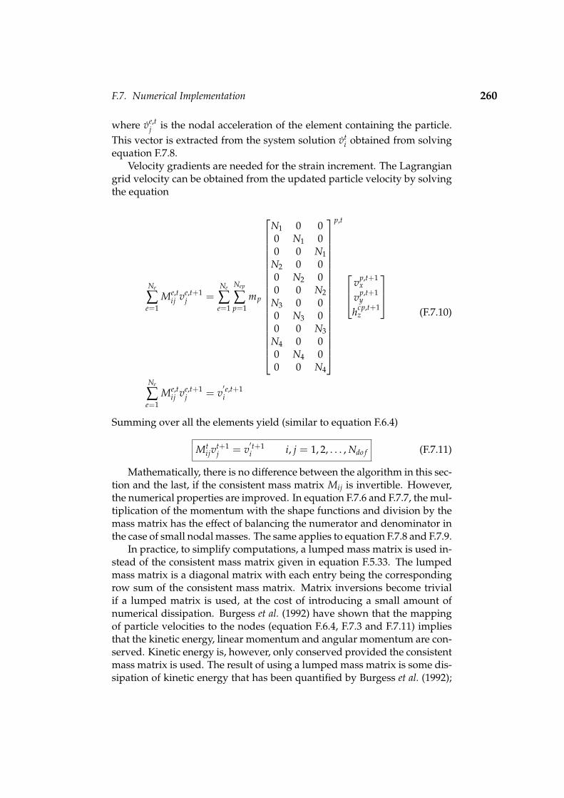
F.7. Numerical Implementation 260
where ve,tj is the nodal acceleration of the element containing the particle.
This vector is extracted from the system solution vti obtained from solving
equation F.7.8.Velocity gradients are needed for the strain increment. The Lagrangian
grid velocity can be obtained from the updated particle velocity by solvingthe equation
Ne
∑e=1
Me,tij ve,t+1
j =Ne
∑e=1
Nep
∑p=1
mp
N1 0 00 N1 00 0 N1
N2 0 00 N2 00 0 N2
N3 0 00 N3 00 0 N3
N4 0 00 N4 00 0 N4
p,t
vp,t+1x
vp,t+1y
hcp,t+1z
Ne
∑e=1
Me,tij ve,t+1
j = v′e,t+1i
(F.7.10)
Summing over all the elements yield (similar to equation F.6.4)
Mtijv
t+1j = v
′t+1i i, j = 1, 2, . . . , Ndo f (F.7.11)
Mathematically, there is no difference between the algorithm in this sec-tion and the last, if the consistent mass matrix Mij is invertible. However,the numerical properties are improved. In equation F.7.6 and F.7.7, the mul-tiplication of the momentum with the shape functions and division by themass matrix has the effect of balancing the numerator and denominator inthe case of small nodal masses. The same applies to equation F.7.8 and F.7.9.
In practice, to simplify computations, a lumped mass matrix is used in-stead of the consistent mass matrix given in equation F.5.33. The lumpedmass matrix is a diagonal matrix with each entry being the correspondingrow sum of the consistent mass matrix. Matrix inversions become trivialif a lumped matrix is used, at the cost of introducing a small amount ofnumerical dissipation. Burgess et al. (1992) have shown that the mappingof particle velocities to the nodes (equation F.6.4, F.7.3 and F.7.11) impliesthat the kinetic energy, linear momentum and angular momentum are con-served. Kinetic energy is, however, only conserved provided the consistentmass matrix is used. The result of using a lumped mass matrix is some dis-sipation of kinetic energy that has been quantified by Burgess et al. (1992);

F.8. Numerical Algorithm 261
Brackbill et al. (1988); Brackbill & Ruppel (1988). The mass matrix can alsobe singular for certain arrangements of the particles. A simple example is asingle particle with unit mass in the center of a computational element. Inone dimension, using linear interpolation, the particle contributed equallyto two vertices. If the element has unit length, the mass matrix is (Burgesset al., 1992)
Meij =
[ 14
14
14
14
](F.7.12)
There appears to be only a few arrangements of particles that yield a singu-lar mass matrix, but nearby arrangements might result in an ill-conditionedmatrix. On the other hand, the lumped matrix is diagonal and well condi-tioned. It is possible to partially lump the mass matrix in order to improvethe numerical computations, at a cost of adding a small amount of dissipa-tion. The partially lumped mass matrix M part lumped
ij is defined as
M part lumpedij = (1− ε) Mij + εM lumped
ij (F.7.13)
When ε = 1, M part lumpedij reduces to the lumped mass matrix M lumped
ij , andwhen ε = 0, it is the full mass matrix Mij. Lumping of the mass matrix hasno effect on the conservation of linear and angular momentum, but doesinfluence the conservation of kinetic energy. Burgess et al. (1992) showedthat for positive ε there is a loss in kinetic energy during grid mapping inthe Lagrangian phase. The dissipation introduced by lumping the massmatrix is O
(∆t2), and this accounts for relatively low energy dissipation
even if ε = 1. Further, Cook et al. (1989, §13.10) showed that explicit timeintegration is usually more accurate with lumped mass matrices than withconsistent mass matrices.
F.8 Numerical Algorithm
This section summarises the numerical algorithm. Assume that at time =t, the position vector, xp,t
i , velocity vector, vp,ti , accumulated strain, ε
cp,ti ,
accumulated stress, σcp,ti and history variables of each particle are known.
The coordinates of the nodes (grid points) are also known. The lists ofelements in entities and particles in elements are known for time = t − 1.

F.8. Numerical Algorithm 262
The different vectors are structured as follows.
xpi =
[xp yp Jp
zzwcpz]T
vpi =
[vp
x vpy hcp
z]T =
[vp
x vpy(
Jpzzwcp
z)]T
εcpi =
[λ
pxx λ
pyy λ
pzz λ
pxy λ
pyx κ
pzxl κ
pzyl]
σcpi =
[σ
pxx σ
pyy σ
pzz σ
pxy σ
pyx
µpzx
lµ
pzy
l
] (F.8.1)
Step 1:
Cycle through all the particles and update the particles-in-element andelement-in-entity lists for time = t. Only the nodes of elements containingparticles will be active nodes during this time step. Set up an array to iden-tify the active nodes on the grid. The total number of degrees-of-freedomNdo f will be three times the number of active nodes (two translational andone rotational degree-of-freedom per node). With the position vector ofa particle and its element known, the particle coordinates in the elementcoordinate system ξη can be calculated. Zhao et al. (1999) developed analgorithm to calculate the element coordinates for four-node bilinear qua-drilateral elements. The ξη-coordinate of each particle is stored since it isused more than once during one time step.
Step 2:
Map the particles momentum to the active nodes to obtain the system nodalmomentum pt
i(
Ndo f × 1)
at time = t.
pti =
Ne
∑e=1
Nep
∑p=1
N1 0 00 N1 00 0 N1
N2 0 00 N2 00 0 N2
N3 0 00 N3 00 0 N3
N4 0 00 N4 00 0 N4
p,t
mpvp,tx
mpvp,ty
mphcp,tz
pti = p
′ti
(F.8.2)

F.8. Numerical Algorithm 263
Step 3:
Calculate the system force vectors. The internal force vector f e int,ti
(Ndo f × 1
)is calculated using the particle stresses at time t and the external force vec-tor f e ext,t
i
(Ndo f × 1
)is calculated using the body forces and surface tracti-
ons. The system consistent mass matrix Mtij(
Ndo f × Ndo f)
is constructedfrom the current particle positions, equation F.5.35. With the force vectorsknown, the rate of change in momentum at time t is simply
pti = f int,t
i + f ext,ti (F.8.3)
Step 4:
With the nodal momentum and the rate of nodal momentum known at timet, the momentum at time t + 1, pt+1
i
(Ndo f × 1
), can be calculated using a
explicit integration scheme.
pt+1i = pt
i + ∆t pti (F.8.4)
Step 5:
The consistent mass matrix can be used, but for simplicity and better nume-rical properties, the lumped or partially lumped mass matrix can be used
M part lumpedij = (1− ε) Mij + εM lumped
ij (F.8.5)
Solving a system of equations is trivial when the lumped matrix is used,but when the consistent or partially-lumped mass matrix is used, specialalgorithms are needed.
Step 6:
To update the particle positions, the updated system nodal velocity,vt+1
i
(Ndo f × 1
), is calculated
vt+1i =
(Mt
ij
)−1pt+1
j (F.8.6)
The particle positions are now updated according to
xp,t+1i = xp,t
i + ∆t Np,tij ve,t+1
j (F.8.7)

F.8. Numerical Algorithm 264
where ve,t+1j (12× 1) are the nodal velocities of the element containing the
particle. This vector is extracted from the system solution vt+1i
(Ndo f × 1
)in equation F.8.6. To update the particle velocity, the updated system nodalacceleration, vt
i(
Ndo f × 1), is calculated
vit =
(Mt
ij
)−1pt
j (F.8.8)
and the velocity update becomes
vp,t+1i = vp,t
i + ∆t Np,tij ve,t
j (F.8.9)
where ve,tj is the nodal acceleration of the element containing the particle.
This vector is extracted from the system solution vti obtained from solving
equation F.8.8.
Step 7:
The grid velocity, vt+1j , is obtained from the updated particle velocity by
solving
Ne
∑e=1
Me,tij ve,t+1
j =Ne
∑e=1
Nep
∑p=1
mp
N1 0 00 N1 00 0 N1
N2 0 00 N2 00 0 N2
N3 0 00 N3 00 0 N3
N4 0 00 N4 00 0 N4
p,t
vp,t+1x
vp,t+1y
hcp,t+1z
Ne
∑e=1
Me,tij ve,t+1
j = v′e,t+1i
Mtijv
t+1j = v
′t+1i
(F.8.10)
Step 8:

F.9. Numerical Integration: Convergence and Stability 265
The strain increment ∆εcpi is calculated at particle positions, using the solu-
tion of equation F.8.10
∆εcpi = ∆t
[vp
x,x vpy,y vp
z,z(vp
x,y + wcpz) (
vpy,x − wcp
z)
wcpz,xl wcp
z,yl]
(F.8.11)
where the velocity derivatives are given by equation F.6.15. With the strainincrement known, a constitutive model can be used to calculate the stressincrement. The strain and stress are then updated according to
εcp,t+1i = ε
cp,ti + ∆ε
cpi (F.8.12)
σcp,t+1i = σ
cp,ti + ∆σ
cpi (F.8.13)
Particle history variables are updated and step 1 repeated to initiate a newtime step.
F.9 Numerical Integration: Convergence and Stability
In the previous sections, a simple forward-difference explicit time integra-tor was used of which the time step should satisfy the stability condition,i.e., the critical time step should be the smallest ratio of the element sizeto the wave speed. For small displacements, the spatial discretisation inPIC is equivalent to that of FEM using Guass points at the same locationsas those of the material points in each cell. Therefore, the convergencebehaviour of the integrator used is similar to that employed to integratethe corresponding equation in FEM. However, no consistent theoretical re-sults have been obtained for the convergence behaviour of time integratorswhen large deformations occur and a reasonable time step is usually foundthrough numerical experiments (Chen et al., 2002).
Wieckowski et al. (1999) pointed out that the PIC method in general mayrequire a shorter time increment than the standard FEM method. The follo-wing stability analysis follows from Wieckowski et al. (1999). In standardFEM, for the one-dimensional element with linear shape functions, the con-dition of stability has the form
∆t ≤ ∆tFEMcrit =
2h√3C
for a consistent mass matrix2h√2C
for a lumped mass matrix(F.9.1)
where h is the element size and C denotes the speed of elastic wave propa-gation. In the PIC method the critical time step, however, depends on themutual position of the material points and the computational mesh. Thecritical time step can be derived from the stability condition
∆t2 ≤ 4mk
(F.9.2)

F.10. Damping 266
where m and k are coefficients in the single homogeneous equation
mu + cu + ku = 0 (F.9.3)
obtained as a result of modal decomposition of the dynamic system ofequations. In the one-dimensional case, for linear elements with one de-gree of freedom, the following expression were obtained for the diagonalterm of the mass matrix
mii =
∑
Npp=1 Mp(ξp)2 for a consistent mass matrix
∑Npp=1 Mpξp for a lumped mass matrix
(F.9.4)
where (1− ξp)h is the distance between the pth material point and the ith
node of the element, h denotes the length of the element, and Np the num-ber of material points in the element. Wieckowski et al. (1999) showed thatthe diagonal term of the element stiffness matrix is
kii =Np
∑p=1
Mp
(Ch
)2
(F.9.5)
where the relation C2 = Eρ is used, with E Young’s modulus and ρ the mate-
rial density. Applying equations F.9.2 to F.9.5, they obtained the followingstability criterion.
∆t ≤ ∆tPICcrit =
2hC
√∑
Npp=1 Mp(ξp)2
∑Npp=1 Mp
for a consistent mass matrix
2hC
√∑
Npp=1 Mpξp
∑Npp=1 Mp
for a lumped mass matrix
(F.9.6)
Comparing equation F.9.6 to equation F.9.1 shows that the value ∆tcrit maybe significantly lower for PIC than for FEM. This is especially true whenthe material points are located near one of the ends (or corners in the two-dimensional case) of the element.
F.10 Damping
In order to obtain static or quasi-static solutions, the equations of motionmust be damped. The objective is to achieve the steady state in a numeri-cally stable way with minimal computational effort. Steady state may beeither equilibrium or steady-flow.
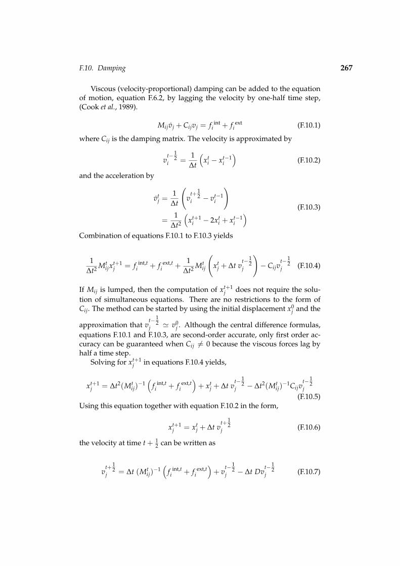
F.10. Damping 267
Viscous (velocity-proportional) damping can be added to the equationof motion, equation F.6.2, by lagging the velocity by one-half time step,(Cook et al., 1989).
Mijvj + Cijvj = f inti + f ext
i (F.10.1)
where Cij is the damping matrix. The velocity is approximated by
vt− 1
2i =
1∆t
(xt
i − xt−1i
)(F.10.2)
and the acceleration by
vtj =
1∆t
(v
t+ 12
i − vt−1i
)
=1
∆t2
(xt+1
i − 2xti + xt−1
i
) (F.10.3)
Combination of equations F.10.1 to F.10.3 yields
1∆t2 Mt
ijxt+1j = f int,t
i + f ext,ti +
1∆t2 Mt
ij
(xt
j + ∆t vt− 1
2j
)− Cijv
t− 12
j (F.10.4)
If Mij is lumped, then the computation of xt+1j does not require the solu-
tion of simultaneous equations. There are no restrictions to the form ofCij. The method can be started by using the initial displacement x0
j and the
approximation that vt− 1
2j ' v0
j . Although the central difference formulas,equations F.10.1 and F.10.3, are second-order accurate, only first order ac-curacy can be guaranteed when Cij 6= 0 because the viscous forces lag byhalf a time step.
Solving for xt+1j in equations F.10.4 yields,
xt+1j = ∆t2(Mt
ij)−1(
f int,ti + f ext,t
i
)+ xt
j + ∆t vt− 1
2j − ∆t2(Mt
ij)−1Cijv
t− 12
j(F.10.5)
Using this equation together with equation F.10.2 in the form,
xt+1j = xt
j + ∆t vt+ 1
2j (F.10.6)
the velocity at time t + 12 can be written as
vt+ 1
2j = ∆t (Mt
ij)−1(
f int,ti + f ext,t
i
)+ v
t− 12
j − ∆t Dvt− 1
2j (F.10.7)

F.10. Damping 268
where D = Ctij(Mt
ij)−1. In order to implement these equations into the algo-
rithm given in section F.8, it must be written in terms of nodal momentum.Multiplying equation F.10.7 by the mass matrix yields
pt+ 1
2i = ∆t pt
i + pt− 1
2i − ∆tDp
t− 12
i
= pt− 1
2i + ∆t
(pt
i − Dpt− 1
2i
) (F.10.8)
which replaces equation F.8.4. Equation F.8.6 becomes
vt+ 1
2i =
(Mt
ij
)−1p
t+ 12
j (F.10.9)
And the particle positional update, equation F.8.7, becomes
xp,t+1i = xp,t
i + ∆t Np,tij v
e,t+ 12
j (F.10.10)
Using equation F.8.8, the velocity update, equation F.8.9, becomes
vp,t+ 1
2i = v
p,t− 12
i + ∆t Np,tij
(ve,t
j − Dvt− 1
2j
)(F.10.11)
The use of velocity-proportional damping, however, involves three maindifficulties (FLAC, 1998):
1. The damping introduces body forces, which are erroneous in flowingregions and may influence the mode of failure in some cases.
2. The optimum damping constant depends on the eigenvalues of thesystem. To calculate the eigenvalues a complete modal analysis mustbe done. In a linear problem, this analysis needs almost as must com-puter effort as the dynamic calculation itself. In nonlinear problems,eigenvalues may be undefined.
3. In its standard form, viscous damping is applied equally to all nodes,i.e., a single damping constant is used throughout the whole system.In many cases, a variety of behaviour may be observed in differentparts of the system. For example, one part may be failing while ano-ther is stable and for these problems, different amounts of dampingare appropriate for different regions.
In order to overcome all three difficulties, a form of damping, called lo-cal non-viscous damping is proposed by FLAC (1998). The damping force ona node is proportional to the magnitude of the unbalanced force at the node.

F.10. Damping 269
The direction of the damping force is such that energy is always dissipated.The damping force is added to the equation of motion, equation F.7.4
pti = f int,t
i + f ext,ti + f damp
i (F.10.12)
where
f dampi = −α
∣∣∣ f int,ti + f ext,t
i
∣∣∣ sign
(p
t− 12
i
)(F.10.13)
f dampi is the damping force and α is the damping constant. The difficulties
reported above are addressed: body forces vanish for steady-state conditi-ons, the magnitude of the damping constant is dimensionless and is inde-pendent of properties or boundary conditions, and the amount of dampingvaries from node to node (FLAC, 1998).

Appendix G
Particle-in-Cell Contact Model
G.1 Introduction
Bardenhagen et al. (2000) developed a PIC model for granular materials thatdescribes both the internal deformation of each granule and the interacti-ons between grains. Interaction between grains is calculated with a contactalgorithm that forbids interpenetration, but allows separation and slidingand rolling with friction. Although this model was developed for an assem-bly of granules, it can be applied to any system of different bodies (entities).
In the basic PIC algorithm, as described in Appendix F, no slip con-tact between different bodies is contained without additional cost. This isthe result of the entities moving in a single-valued velocity field v. Sincethis velocity field is determined using mass weighting, Bardenhagen et al.(2000) calls it the centre-of-mass velocity field. Here it will be called the sys-tem velocity field since all the particles in the system are used to calculate it.The solution procedure described in Appendix F can also be followed, butwhere the loops range over only the particles making up one entity. Thiswould solve the equations of motion for each entity, ignoring the presenceof all the others. In that case, the result is a single-valued entity velocityfield v ent.
Obviously, the entity motion cannot be determined solely from consi-deration of each individual entity in isolation. The novelty here is (Barden-hagen et al., 2000) that contacts between entities are handled by comparingthe velocity fields v ent to the single, system velocity field v. The resultingalgorithm is linear in the number of entities and requires no iteration.
Matrix tensor notation (Hassenpflug, 1993) is used for clarity and subs-cripts should not be confused with the indices of index notation.
G.2 Contact Model
Normal and tangential kinematic constraints on the velocity are handledseparately. Suppose that the boundary of each entity has been identifiedand the unit outward normal nb
ent is known at nodes along the boundary(the subscript b indicates that it is a value/property at boundary node b). Ifone entity is isolated from the rest, i.e. not in contact with others, then thetwo velocity fields v ent and v will be identical in the neighbourhood of thatentity. It is only as the entity approaches other entities that the two fieldswill differ. Contact is then defined when these two velocity fields differ.Constraints are only necessary when entities are approaching each other
270

G.2. Contact Model 271
and not when they are moving apart from one another. The following con-dition is used to check whether an entity is in contact with another entityand whether they are approaching each other.(
vbent − vb
)• nb
ent > 0 (G.2.1)
This condition is satisfied when the entity velocity, at a boundary node, isovertaking the system velocity along the normal to the surface. Once thiscondition is satisfied, the entity velocity is adjusted to a new value vb
˜ ent sothat
vb˜ ent • nb
ent = vb • nbent (G.2.2)
holds. Equation G.2.2 states that the normal of the entity velocity is setequal to the normal component of the system velocity. Equation G.2.2 canalso be written as
vb˜ ent = vb
ent −[(
vbent − vb
)• nb
ent] nbent (G.2.3)
To prove equation G.2.3, take the scalar product on each side of the equalsign with respect to the unit normal nb
ent.
vb˜ ent • nb
ent =[vb
ent −[(
vbent − vb
)• nb
ent] nbent] • nb
ent
= vbent • nb
ent −(vb
ent − vb)• nb
ent
= vbent • nb
ent − vbent • nb
ent + vb • nbent
= vb • nbent
(G.2.4)
The system velocity does not allow interpenetration of entities, so this choiceof a contact constraint in the normal direction is natural. Note that the in-equality in equation G.2.1 allows entities to separate freely without anyconstraints. The constraint in equation G.2.2 is equivalent to applying a
normal force fbent,normal
to the entity boundary node
fbent,normal
= −Ment
b∆t
[(vb
ent − vb)• nb
ent] nbent
=Ment
b∆t
[(vb˜ ent − vb
ent) • nbent] nb
ent(G.2.5)
where Mentb is the entity mass at boundary node b. This mass is the value
of the entity lumped mass matrix at this node. The entity mass matrix iscalculated summing only over the entity’s particles.
If there is no contact friction between the entities, then the above ad-justment of the normal component of the entity velocity, equation G.2.3, isall that is required. The tangential component of the entity velocity willbe unconstrained. This can be proven by writing down the expression for

G.2. Contact Model 272
x
y
Node b
bv
entbv
bn
( )bent
b vv −
( )[ ] entb
entbb
entb nnvv •−
( ) ( )[ ] entb
entbb
entbb
entb nnvvvv •−−−
tbθ
Figure G.1: System, entity and relative velocities
the corrected tangential entity velocity. Using equation G.2.2 and equa-tion G.2.3,
vb˜ ent −
(vb˜ ent • nb
ent) nbent = vb
ent −(vb
ent • nbent) nb
ent (G.2.6)
it is shown that the tangential component of the corrected entity velocity isthe same as the tangential component before the correction was applied.
Where equation G.2.1 is based on the relative normal velocity, the tan-gential contact constraint is based on the relative tangential velocity givenby (Figure G.1) (
vbent − vb
)−[(
vbent − vb
)• nb
ent] nbent (G.2.7)
This tangential velocity vector can also be written making use of cross pro-ducts.
nbent ×
[(vb
ent − vb)× nb
ent] (G.2.8)
To prove this equation, first look at the second cross product, using thedefinition thereof (AppendixA.2.6)[(
vbent − vb
)× nb
ent] = |(vb
ent − vb)| sinθ ez (G.2.9)
where θ is the angle between the two vectors, figure G.1, and ez is the unitvector in the z-direction, i.e., the out-of-plane direction. Looking at the firstcross product, the vector can be written as
nbent ×
[(vb
ent − vb)× nb
ent] = |(vb
ent − vb)
sinθ| sin π2 tb
= |(vb
ent − vb)
sinθ| tb(G.2.10)

G.2. Contact Model 273
since the angle between nb and ez is 90 and tb is the tangential unit vectorat the contacting node. Making use of figure G.1, sinθ can be written as
sinθ =(vb
ent − vb
)−[(
vbent − vb
)• nb
ent] nbent(
vbent − vb
) (G.2.11)
Substitution of this definition into equation G.2.10 leads to
nbent ×
[(vb
ent − vb)× nb
ent] = |(vb
ent − vb)−[(
vbent − vb
)• nb
ent] nbent| tb
=(vb
ent − vb)−[(
vbent − vb
)• nb
ent] nbent
(G.2.12)which concludes the proof.
To apply Coulomb friction, first calculate the force required for no slip.Again the comparison of the entity velocity to the system velocity providesthe correct constraint for no slip contact, in the form of the relative tangen-
tial velocity, equation G.2.7. The constraining tangential force, fbent,stick
, tocause the entities to stick, is
fbent,stick
= −Ment
b∆t
nbent ×
[(vb
ent − vb)× nb
ent] (G.2.13)
The friction force equals the sticking force if the magnitude of the stickingforce is small. That is, friction just balances the tangential force and pre-vents relative tangential motion, when the magnitude of the tangentialforce is small. For larger tangential forces, the magnitude of the frictionforce is proportional to the magnitude of the normal force and independentof the contact area. The proportionality constant (friction coefficient) is µ.Limiting the frictional force to have magnitude less than the sticking forceallows tangential slip between contacting entities since the applied frictio-nal force is not sufficient to prevent relative tangential motion, figure G.2.The direction of the frictional force is chosen as in equation G.2.13 to op-pose relative motion. Putting all these requirements together yields
fbent, f ric
=fb
ent,stick∣∣∣ fbent,stick
∣∣∣ min(
µ∣∣∣ fb
ent,normal∣∣∣ ,∣∣∣ fb
ent,stick∣∣∣) (G.2.14)
Using equation G.2.13 it can be shown that
fbent,stick∣∣∣ fbent,stick
∣∣∣ =−Ment
b∆t nb
ent ×[(
vbent − vb
)× nb
ent]∣∣∣Mentb
∆t nbent ×
[(vb
ent − vb
)× nb
ent]∣∣∣= −
nbent ×
[(vb
ent − vb
)× nb
ent]∣∣(vbent − vb
)× nb
ent∣∣
(G.2.15)
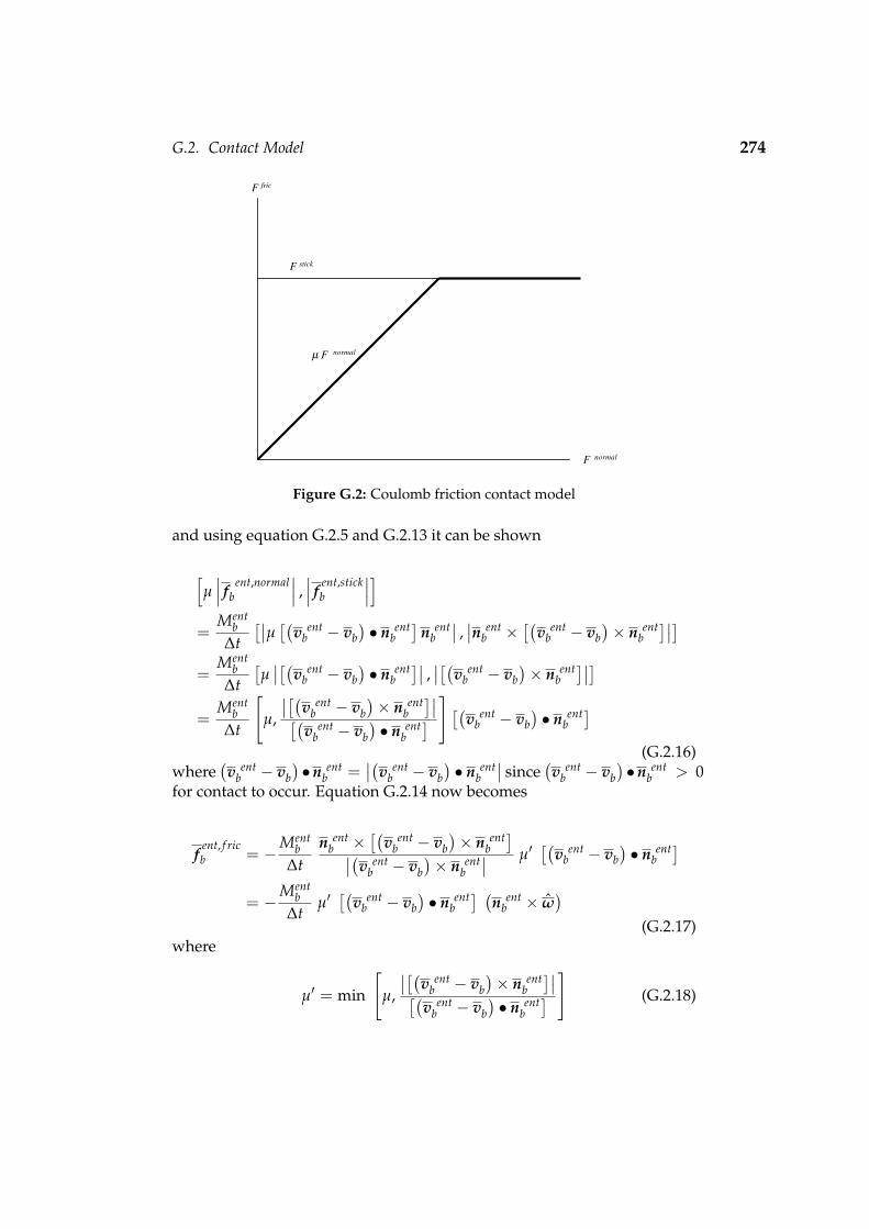
G.2. Contact Model 274
F normal
F fric
F stick
µ F normal
Figure G.2: Coulomb friction contact model
and using equation G.2.5 and G.2.13 it can be shown
[µ∣∣∣ fb
ent,normal∣∣∣ ,∣∣∣ fb
ent,stick∣∣∣]
=Ment
b∆t
[∣∣µ [(vbent − vb
)• nb
ent] nbent∣∣ ,
∣∣nbent ×
[(vb
ent − vb)× nb
ent]∣∣]=
Mentb
∆t[µ∣∣[(vb
ent − vb)• nb
ent]∣∣ ,∣∣[(vb
ent − vb)× nb
ent]∣∣]=
Mentb
∆t
[µ,
∣∣[(vbent − vb
)× nb
ent]∣∣[(vb
ent − vb
)• nb
ent]] [(
vbent − vb
)• nb
ent](G.2.16)
where(vb
ent − vb
)•nb
ent =∣∣(vb
ent − vb
)• nb
ent∣∣ since
(vb
ent − vb
)•nb
ent > 0for contact to occur. Equation G.2.14 now becomes
fbent, f ric
= −Ment
b∆t
nbent ×
[(vb
ent − vb
)× nb
ent]∣∣(vbent − vb
)× nb
ent∣∣ µ′
[(vb
ent − vb)• nb
ent]= −
Mentb
∆tµ′[(
vbent − vb
)• nb
ent] (nbent × ω
)(G.2.17)
where
µ′ = min
[µ,
∣∣[(vbent − vb
)× nb
ent]∣∣[(vb
ent − vb
)• nb
ent]]
(G.2.18)
G.2. Contact Model 275
and the unit vector ω is
ω =[(
vbent − vb
)× nb
ent]∣∣(vbent − vb
)× nb
ent∣∣ (G.2.19)
Similarly to where equation G.2.3 is the only correction needed for normalcorrection, the result from equation G.2.17 can be used to write a correctedvelocity taking only the tangential correction into account.
vb˜ ent = µ′
[(vb
ent − vb)• nb
ent] (nbent × ω
)(G.2.20)
Finally, imposing both the frictional constraint force and the normal cons-traint force, the altered entity velocity is
vb˜ ent = vb
ent −[(
vbent − vb
)• nb
ent] (nbent + µ′ nb
ent × ω)
(G.2.21)
This equation is simply a vector sum of equation G.2.3 and equation G.2.20.To obtain a no-slip contact, using equation G.2.21, the friction coefficient µshould be given a high value.
In order to implement these equations efficiently, the following defini-tions are made (the subscript b being omitted for clarity): The difference invelocity is defined by vdi f f
v di f f ≡[
v di f fx
v di f fy
]= v ent − v =
[v ent
x − vxv ent
y − vy
](G.2.22)
The scalar (dot) product of the velocity difference with the unit normal vec-tor is as follows
D = v di f fx n ent
x + v di f fy n ent
y (G.2.23)
The vector (cross) product of the two same vectors can be shown to be
C =
00
v di f fx n ent
y − v di f fy n ent
x
(G.2.24)
Note that this results in only an out-of-plane (z-direction) component, theabsolute value of this vector being
∣∣C∣∣ =∣∣∣v di f f
x n enty − v di f f
y n entx
∣∣∣. The unitvector ω can be shown to have the form
ω =C∣∣C∣∣ =
00
v di f fx n ent
y −v di f fy n ent
x∣∣∣v di f fx n ent
y −v di f fy n ent
x
∣∣∣
(G.2.25)

G.3. Boundary Unit Normal Vector Calculation 276
Equation G.2.18 will simply be
µ′ = min
[µ,
∣∣C∣∣D
](G.2.26)
which is, of course, a scalar quantity. Equation G.2.21 can now be writtenas
[v ent
xv ent
y
]=[
v entx
v enty
]− D
[n entx
n enty
]+ µ′
n ent
y
(v di f f
x n enty −v di f f
y n entx
)|C|
−n entx
(v di f f
x n enty −v di f f
y n entx
)|C|
(G.2.27)where only the first two components are shown since the out-of-plane com-ponent is zero, as expected. Thus, after calculation of the components ofvdi f f , D,
∣∣C∣∣ and µ′, equation G.2.27 can be used to calculate each of thenew nodal velocity components individually.
Using a polar continuum, each node has two translational velocitiesand one rotational velocity. The translational velocities are corrected inthe same way as above, while the rotation is either set to be zero at thecontacting nodes or free, i.e. not constraint or changed.
G.3 Boundary Unit Normal Vector Calculation
Sulsky & Brackbill (1991) proposed a method for calculating the divergenceof a vector quantity and the gradient of a scalar quantity at grid points. Thederivations are done for the two-dimensional case, but in general, the sameprocedure can be followed for the three-dimensional case. For each entity,the particle mass is interpolated to the finite element centres, xc and dividedby the element volume Ve, to obtain a density.
ρc =1Ve
Nep
∑p=1
mpS(1)(xc − xp) (G.3.1)
The shape function S(1) is constructed from bilinear b-splines (Dierckx,1996; Piegl and Tiller, 1997). The gradient of ρc evaluated at the nodes of thecomputational mesh provides the normal direction at the surface of eachentity. The interaction between entities is therefore not along a commonnormal, which results in small errors in momentum conservation (Barden-hagen et al., 2000).
Let xi,j, xi+1,j, xi+1,j+1, xi,j+1 denote the vertices of the computational ele-ment (i, j), figure G.3. With natural (element) coordinates (ξ, η) which as-

G.3. Boundary Unit Normal Vector Calculation 277
jix , jix ,1+
1,1 ++ jix
1, +jix
ξ
η
1 2
3
4
Figure G.3: Computational element with numbered vertices
sume integer values at the vertices and using bilinear interpolation, anypoint x in the element is given by
x = ξ ′[(
1− η′)
xi+1,j + η′xi+1,j+1
]+(1− ξ ′
) [(1− η′
)xi,j + η′xi,j+1
](G.3.2)
with ξ ′1 = ξ1− i and η′ = η− j. This mapping can also be written as (Sulskyand Brackbill, 1991)
x =Nen
∑n=1
xns(1) (ξ − i, η − j) (G.3.3)
where Nen is the number of nodes (vertices) per element, xn is the nodecoordinates and
s(1) (ξ − i, η − j) = s(1) (ξ ′, η′)
= (1− |ξ|) (1− |η|) (G.3.4)
A corresponding interpolation function in physical coordinates can be writ-ten for a rectangular element
S(1) (x) = S(1) (x, y) =(
1− |x|∆x
)(1− |y|
∆y
)(G.3.5)
where ∆x and ∆y are the element size in the x and y directions respectively.Make use of a vector u = [ux uy]T (known at the nodes), which can be avelocity vector, acceleration vector or any other vector field, to derive thenecessary equations. A derivative of a nodal variable results in an element-centred quantity and is calculated as an average over the element. The

G.3. Boundary Unit Normal Vector Calculation 278
average of the derivative of the x-component of u with respect to the x-coordinate is
〈∂ux
∂x〉
c≡ 1
Ve
∫Ve
∂ux
∂xdV (G.3.6)
where the subscript c indicates that the average derivative is an element-centred value. To evaluate equation G.3.6, make use of equation G.3.3 andG.3.5. Define u throughout the cell from its values at the nodes
u(x, t) =Nen
∑n=1
unS(1) (x− xn) (G.3.7)
To evaluate equation G.3.6, we need the element-centred quantity whichcan be written as
u(xc, t) =Nen
∑n=1
unS(1) (xc − xn) (G.3.8)
Now equation G.3.6 becomes
〈∂ux
∂x〉
c=
1Ve
∫Ve
Nen
∑n=1
uxn∂
∂xS(1) (xc − xn) dV
=1Ve
Nen
∑n=1
uxnccvx
(G.3.9)
where
ccvx =
∫Ve
∂
∂xS(1) (xc − xn) dV (G.3.10)
Since equation G.3.9 is summed over all the nodes of the element, there willbe Nen ccv
x values, one for each node.An equation similar to equation G.3.9 can be written for the derivative
with respect to the y-coordinate. This will result in Nen ccvy coefficients. It
is useful to form a vector ccv = [ccvx ccv
y ]T of the geometric coefficients. Onecan now combine derivatives to form a discrete divergence operator, actingon nodal quantities and defined at the cell centre.
Dc(un) =1Ve
∫Ve
∇ • u dV =1Ve
Nen
∑n=1
ccv • un (G.3.11)
In the same way, derivatives are combined to form a discrete gradient ope-rator defined at an element centre
Gc(ρn) =1Ve
∫Ve
∇ρ dV =1Ve
Nen
∑n=1
ccvρn (G.3.12)
G.3. Boundary Unit Normal Vector Calculation 279
where ρ is a scalar quantity and not a vector like u. We now have formulasfor the divergence and gradient, acting on element nodal data defined atthe element centre. The "inverse" will now be constructed, i.e. formulasfor divergence and gradient operators, acting on element-centred data andlocated at the nodes. These formulas are constructed to satisfy a discreteform of the divergence theorem (Sulsky and Brackbill, 1991)∫
Sρu • n dS =
∫V
∇ • (ρu) dV
=∫
Vu •∇ρ dV +
∫V
ρ∇ • u dV(G.3.13)
where we assume that u is defined at nodes and ρ defined at element cen-tres. An approximation for the last term in equation G.3.13 is already defi-ned in equation G.3.11
∑e∈V
ρcDc(un)Ve = ∑e∈V
ρc
Nen
∑n=1
ccv • un (G.3.14)
where the sum ∑e∈V is over all the elements in V. At this point, postulate aform for the gradient at a vertex (Sulsky and Brackbill, 1991) analogous toequation G.3.12.
VnGn(ρc) = ∑e
ccvρc (G.3.15)
where the components of the geometric coefficients ccvare still unknown.The control volume Vn centred at a node xn is given by
Vn = 14 ∑
eVe (G.3.16)
The sum in equation G.3.15 and equation G.3.16 is over all the elementse that have xn as a node. Combining equations G.3.13, G.3.14 and G.3.15yields
∫S
ρu • n dS = ∑n∈V
un •∑e
ccvρc + ∑e∈V
ρc
Nen
∑n=1
ccv • un
= ∑n∈V
un •∑e
(ccv + ccv) ρc
(G.3.17)
where ∑n∈V is the sum over all the nodes in the control volume V. The lefthand side of equation G.3.17 is a surface integral, so the right-hand sideshould only involve nodes on the boundary of V. Since u and ρ are arbi-trary, for any interior element e we need the integral in equation G.3.17 to

G.3. Boundary Unit Normal Vector Calculation 280
vanish, i.e. ccv = − ccv. The required formula for a gradient operator actingon a centred quantity, defined at the nodes follows from equation G.3.15
VnGn(ρc) = − ∑e
ccvρc (G.3.18)
To obtain the formula for the divergence at a node, the process is similar.Start with equation G.3.13, but now let u be defined at element centres, let ρbe a nodal quantity and let V be a union of node-centred control volumes.Use equation G.3.12 to define an approximation to the first term on theright-hand side of equation G.3.13, and proceed as above to obtain
VnDn(uc) = − ∑e
ccv • uc (G.3.19)
Applying the gradient operator, equation G.3.18, to the element-centreddensity defined in equation G.3.1, the result is a vector approximately nor-mal to the entity surface at node n.
All that remains is to calculate the components of the geometric coeffi-cient vector ccv. The coefficients are defined by equation G.3.10.
ccvx =
∫Ve
∂
∂xS(1) (xc − xn) dV
ccvy =
∫Ve
∂
∂yS(1) (xc − xn) dV
(G.3.20)
The derivatives of S(1), equation G.3.5, for a rectangular element (figure G.4)with respect to the x- and y-coordinates are
∂S(1)(x, y)∂x
=−sign(x)
∆x
(1− |y|
∆y
)∂S(1)(x, y)
∂y=−sign(y)
∆y
(1− |x|
∆x
) (G.3.21)
The value of ccvx for node 1 follows as
ccvx1 =
∫Ve
∂
∂xS(1) (xc − x1) dV
=∫
Ve
−sign(xc − x1)∆x
(1− |yc − y1|
∆y
)dV
=∫
Ve
−1∆x
(1− ∆y
2∆y
)dV
=−12∆x
∆x∆y
=−∆y
2
(G.3.22)

G.3. Boundary Unit Normal Vector Calculation 281
1 2
34
( )11, yx ( )22 , yx
( )44 , yx ( )33, yx
x∆
y∆( )cc yx ,
Figure G.4: Rectangular computational element
Table G.1: Geometric coefficients for a rectangular element
Node n ccvx ccv
y
1 −∆y2 −∆x
2
2 ∆y2 −∆x
2
3 ∆y2
∆x2
4 −∆y2
∆x2
where ∆x∆y is the volume of the element (unit thickness is assumed). Ta-ble G.1 summarises the results by following the same procedure for theother nodes and the y-derivatives.
As an example, consider figure G.5 where node n has been identified asa boundary node. Elements 1, 2 and 3 are boundary elements and containnode n as one of their vertices. Assume that the element centre densities,equation G.3.1, have been calculated. Applying equation G.3.18 to node nthen gives
VnGn(ρc) = − ∑e
ccvρc
= − (c3cvρc1 + c4
cvρc2 + c2cvρc3)
= −([
ccvx3
ccvy3
]ρc1 +
[ccv
x4ccv
y4
]ρc2 +
[ccv
x2ccv
y2
]ρc3
) (G.3.23)
Since Vn is only a scalar quantity and the gradient vector needs to be nor-malised to obtain the unit normal vector, it can be discarded and the unit

G.4. Implementation 282
1 12
3
4 3 4 3
2
1
4
2
ρc1 ρc2
ρc3
n
nn
Figure G.5: Example of boundary unit normal calculation
normal vector follows as
nn =[
nnxnny
]=−([
ccvx3
ccvy3
]ρc1 +
[ccv
x4ccv
y4
]ρc2 +
[ccv
x2ccv
y2
]ρc3
)∣∣∣∣([ccv
x3ccv
y3
]ρc1 +
[ccv
x4ccv
y4
]ρc2 +
[ccv
x2ccv
y2
]ρc3
)∣∣∣∣ (G.3.24)
G.4 Implementation
In section F.8 the numerical algorithm is summarised. Equation F.8.6 givesthe system nodal velocity vt+1
i at time t + 1. The same procedure is thenfollowed for each entity to obtain an entity nodal velocity vent,t+1
i . In thisanalysis the summation is performed only over particles belonging to theentity in question. Each active node will now have at least two velocityvectors. One system velocity vector and at least one entity velocity vector.If there are particles of more than one entity in the same element, the nodesof this element will have a velocity vector for each entity as well as thesystem velocity.
At this stage in the calculation the boundary nodes of each entity areidentified. The entity velocity field is then compared to the system velocityfield at the boundary nodes. Contact is defined by equation G.2.1 and a cor-rection, equation G.2.21, is made to the entity nodal velocity if necessary.The corrected entity velocity is used to update the entity’s particles accor-ding to equation F.8.7. To update the particle velocity, the new accelerationfirst needs to be calculated.
˙v ent,t+1i =
v ent,t+1i − v ent,t
i∆t
(G.4.1)
The entity’s particle velocity is then updated according to equation F.8.9.
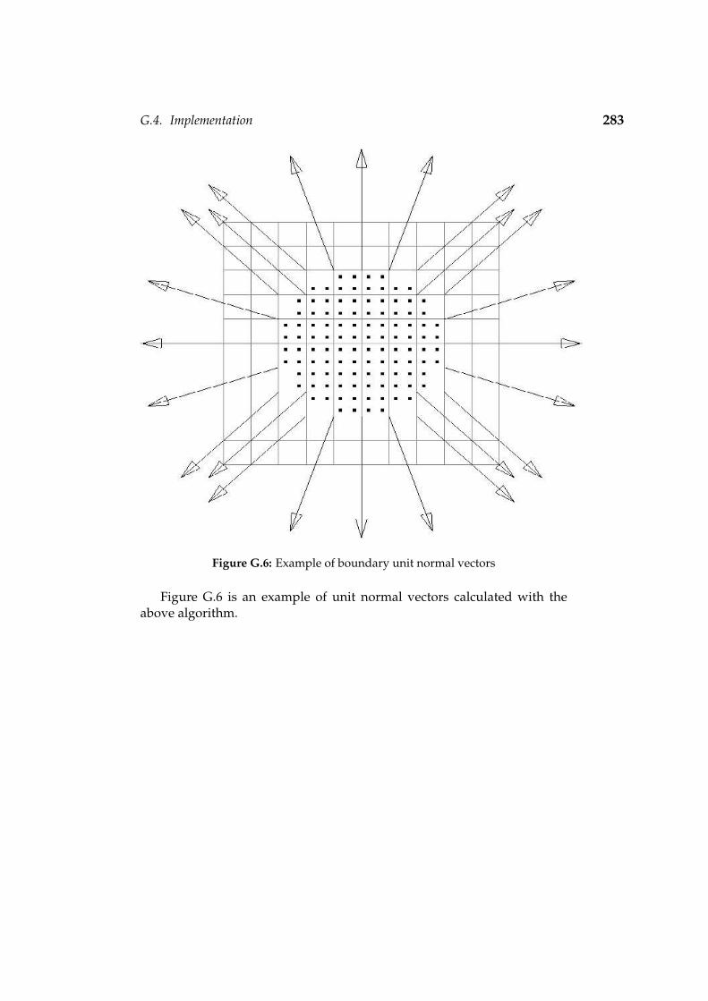
G.4. Implementation 283
Figure G.6: Example of boundary unit normal vectors
Figure G.6 is an example of unit normal vectors calculated with theabove algorithm.

Appendix H
Nonpolar Constitutive Models andImplementation
H.1 Introduction
In this appendix, the different nonpolar constitutive models employed aredescribed. These include
1. Elastic, Isotropic Model
2. Drucker-Prager Model
3. von Mises Model
4. Mohr-Coulomb Model
The formulation given in this appendix closely follows that of FLAC(1998).
H.2 Elastic, Isotropic Model
These stress-strain laws are linear and path independent. The incrementalrelation between stress and strain is expressed by Hook’s law for the casesof plane strain and plane stress.
H.2.1 Plane Strain
∆σ11 = α1∆ε11 + α2∆ε22
∆σ22 = α2∆ε11 + α1∆ε22
∆σ12 = ∆σ21 = 2G∆ε12 = 2G∆ε21
∆σ33 = α2 (∆ε11 + ∆ε22)
(H.2.1)
where
α1 = K + 43 G
α2 = K− 23 G
K =E
3 (1− 2ν)= bulk modulus
G =E
2 (1 + ν)= shear modulus
(H.2.2)
with E Young’s modulus and ν Poisson’s ratio.
284

H.3. Drucker-Prager Model 285
H.2.2 Plane Stress
∆σ11 = β1∆ε11 + β2∆ε22
∆σ22 = β2∆ε11 + β1∆ε22
∆σ12 = ∆σ21 = 2G∆ε12 = 2G∆ε21
∆σ33 = 0
(H.2.3)
where
β1 = α1 −(
α22
α1
)β2 = α2 −
(α2
2α1
) (H.2.4)
H.3 Drucker-Prager Model
The different plastic models are characterised by their yield function, har-dening/softening functions and the flow (potential function) rule. Theyield function defines the stress combination for which plastic flow takesplace. These functions or criteria are represented by one or more limitingsurfaces in a generalised stress space with points below or on the surfacebeing characterised by an incremental elastic or plastic behaviour, respec-tively. The plastic flow formulation rests on the basic assumptions fromplasticity theory that the total strain increment may be decomposed intoelastic and plastic parts, with only the elastic part contributing to the stressincrement by means of an elastic law. The flow rule specifies the direc-tion of the plastic strain increment vector as the normal to the potentialsurface. It is called associated if the potential and yield functions coincideand non-associated otherwise. See Vermeer & De Borst (1984), Mendelson(1968) and Blazynski (1983) for more detail on the theory of plasticity andassociated and non-associated flow rules.
The Drucker-Prager model consists of a Drucker-Prager yield criterionwith tension cutoff. The shear flow rule is non-associated and the tensileflow rule is associated.
H.3.1 Incremental Elastic Law
The model is expressed in terms of two generalised stress components: thetangential stress q and mean normal stress p defined as
q =√
J2
p = 13 (σ11 + σ22 + σ33)
(H.3.1)

H.3. Drucker-Prager Model 286
where J2 is the second invariant of the stress deviator tensor, expressed as(Mendelson, 1968)
J2 = 16
[(σ11 − σ22)
2 + (σ22 − σ33)2 + (σ11 − σ33)
2 + 6(σ2
12 + σ223 + σ2
31)]
(H.3.2)for a nonpolar continuum. Under the assumption of plane strain J2 beco-mes
J2 = 16
[(σ11 − σ22)
2 + (σ22 − σ33)2 + (σ11 − σ33)
2]+ σ2
12 (H.3.3)
The shear strain increment ∆εq and volumetric strain increment ∆εp asso-ciated with q and p respectively, have the form
∆εq = 2√
∆J′2∆εp = ∆ε11 + ∆ε22 + ∆ε33
(H.3.4)
where ∆J′2 is the second invariant of the incremental strain deviator tensor,given by
∆J′2 = 16
[(∆ε11 − ∆ε22)
2 + (∆ε22 − ∆ε33)2 + (∆ε11 − ∆ε33)
2]+ ∆ε2
12
(H.3.5)The strain components are decomposed in elastic and plastic parts.
∆εq = ∆εeq + ∆ε
pq
∆εp = ∆εep + ∆ε
pp
(H.3.6)
where the superscript e and p refer to elastic and plastic parts respectively.The incremental expression of Hook’s law in terms of generalised stressesand strains is (Kachanov, 1971; Johnson and Mellor, 1983)
∆q = G∆εeq
∆p = K∆εep
(H.3.7)
with G and K the shear and bulk modulus respectively.
H.3.2 Yield and Potential Functions
The failure (yield) criteria are described in the pq-plane, figure H.1. Frompoint A to B the criterion is defined by the Drucker-Prager shear yield func-tion
f s = q + qφ p− kφ (H.3.8)

H.3. Drucker-Prager Model 287
A
B
C
0=sf
0=tf
φk
tσ
φ
φ
q
k
+
-
+-
-
+
0=h
domain 1
domain 2
p
q
Figure H.1: Drucker-Prager failure criterion
and from B to C by the tension yield function (tension cutoff)
f t = p− σt (H.3.9)
where qφ and kφ are constant material properties and σt is the tensile strengthfor the Drucker-Prager model. This value is defined as the maximum of themean normal stress for the material. For a material whose qφ is not equalto zero, the tensile strength cannot exceed the maximum value σt
max givenby (figure H.1)
σtmax =
kφ
qφ(H.3.10)
The default value of the tensile strength σt is zero if the material propertyqφ is zero. The shear potential function gs corresponds in general to a non-associated flow rule and has the form
gs = q + qψ p (H.3.11)
where qψ is a material constant, equal to qφ if the flow rule is associated.The flow rule for tensile failure is associated. It is given by
gt = p (H.3.12)
The flow rules are given a unique definition (FLAC, 1998) in the vicinityof an edge of the composite yield function, point B in figure H.1. A functionh(p, q) = 0 is defined which is represented by the diagonal between the
H.3. Drucker-Prager Model 288
representation of f s = 0 and f t = 0 in the pq-plane. This function is givenby
h = q− τp − αp(p− σt) (H.3.13)
where τp and αp are two constants defined as
τp = kφ − qφσt
αp =√
1 + q2φ − qφ
(H.3.14)
An elastic guess violating the failure criterion is represented by a point inthe pq- plane located either in domain 1 or 2, corresponding to positive ornegative values of h, respectively. If in domain 1, shear failure is declared,and the stress point is brought back to the curve f s = 0 using a flow rulederived using the potential function gs. If in domain 2, tensile failure ta-kes place and the stress point is brought back to f t = 0 using a flow rulederived using gt.
H.3.3 Plastic Corrections
First consider shear failure. The flow rule has the form
∆εpq = λs ∂gs
∂q
∆εpp = λs ∂gs
∂p
(H.3.15)
where the magnitude of the parameter λs remains to be defined. Usingequation H.3.11 for gs, these expressions give, after partial differentiation
∆εpq = λs
∆εpp = qψλs (H.3.16)
Using equation H.3.6, the elastic strain increments may be expressed as thetotal strain increment minus the plastic increment.
∆εeq = ∆εq − ∆ε
pq
= ∆εq − λs
∆εep = ∆εp − ∆ε
pp
= ∆εp − qψλs
(H.3.17)
The increment in generalised stress can now be written, using Hook’s law,equation H.3.7
∆q = G∆εq − Gλs
∆p = K∆εp − Kqψλs (H.3.18)

H.3. Drucker-Prager Model 289
σ0
σn
σt
ε0 εn
σ
ε
∆ε
∆σ
∆ε p∆ε eE
1
Figure H.2: One-dimensional representation of elasto-plastic relation
The new stress state is given by
qN = qO + ∆q
pN = pO + ∆p(H.3.19)
where the superscripts N and O refer to the new and old stress states re-spectively. Substitution of equation H.3.18 into equation H.3.19 leads to
qN =(
qO + G∆εq
)− Gλs
= qI − Gλs
pN =(
pO + K∆εp
)− Kqψλs
= pI − Kqψλs
(H.3.20)
where the superscript I is used to represent the elastic guess obtained byadding to the old stress, elastic increments computed using the total strainincrement, figure H.2.
The new stress point should be located on the shear yield surface. Usingthis, the parameter λs can be calculated by substitution of qN and pN for qand p in f s = 0. Using equation H.3.8 and equation H.3.20, and after some

H.3. Drucker-Prager Model 290
manipulation, λs is given by
λs =f s (pI , qI)
G + Kqφqψ(H.3.21)
With the new generalised stresses known, the new stress tensor needs tobe calculated. Noting that the new deviatoric stresses may be obtained bymultiplying the corresponding deviatoric elastic guess with the ratio qN
qI ,the new stresses may be written as (FLAC, 1998)
σNij =
(σI
ij − pIδij
) qN
qI + pNδij (H.3.22)
where δij is the Kronecker delta symbolFor tensile failure, the same procedure is followed. The flow rule has
the form
∆εpq = λt ∂gt
∂q
∆εpp = λt ∂gt
∂p
(H.3.23)
Using equation H.3.12 for gt, these plastic strain increments become
∆εpq = 0
∆εpp = λt (H.3.24)
The increments in elastic strains become
∆εeq = ∆εq − ∆ε
pq
= ∆εq
∆εep = ∆εp − ∆ε
pp
= ∆εp − λt
(H.3.25)
Using Hook’s law, the increments in stress become
∆q = G∆εq
∆p = K∆εp − Kλt (H.3.26)
The new stress states are given by equation H.3.19. Using this equation and

H.3. Drucker-Prager Model 291
equation H.3.26, the new stress states are given by
qN =(
qO + G∆εq
)= qI
pN =(
pO + K∆εp
)− Kλt
= pI − Kλt
(H.3.27)
The parameter λt is calculated, using f t = 0
λt =pI − σt
K(H.3.28)
Substitution of this equation in equation H.3.27 yields
qN = qI
pN = σt (H.3.29)
In the tensile mode of failure the new deviatoric stresses correspond tothe elastic guess
(qN
qI = 1)
and the new stress tensor follows as
σNij = σI
ij +(
σt − pI)
δij (H.3.30)
H.3.4 Implementation Procedure
In this section describes the implementation of the Drucker-Prager modelin the numeric code.
Step1:
Calculate an elastic guess σIij. This is done by assuming that the total strain
increment is elastic. For the case of plane strain, equation H.2.1 is used.
Step2:
Calculate the generalised stress components(
pI , qI) using the elastic guessσI
ij and equation H.3.1 and H.3.3. If these stresses violate the compositeyield criterion (equation H.3.8 and H.3.9), a correction must be applied tothe generalised stress components to give the new stress state. The yieldcriteria is violated if f s >= 0 or f t >= 0. The function h (equation H.3.13)is used to determine if shear failure or tensile failure has occurred, i.e.h(pI , qI) > 0 or h(pI , qI) ≤ 0 respectively.

H.4. The von Mises Model 292
Step3a:
If shear failure is declared, new generalised stresses are calculated fromequation H.3.20 using equation H.3.21 for λs.
Step3b:
If tensile failure is declared, new generalised stresses are calculated fromequation H.3.27 using equation H.3.28 for λt.
Step4a:
In the case of shear failure the stress tensor components in the system ofreference axes are calculated from the corrected generalised stresses usingequation H.3.22.
Step4b:
In the case of tensile failure the stress tensor components in the system ofreference axes are calculated from the corrected generalised stresses usingequation H.3.30.
H.4 The von Mises Model
The von Mises yield criterion is also known as the distortion energy theory.It assumes that yielding begins when the distortion energy equals the dis-tortion energy at yield in simple tension (Mendelson, 1968). The yield con-dition is given by
12
[(σ11 − σ22)
2 + (σ22 − σ33)2 + (σ11 − σ33)
2 + 6(σ2
12 + σ223 + σ2
31)]
= σ2y
(H.4.1)And under the assumption of plane strain this becomes
12
[(σ11 − σ22)
2 + (σ22 − σ33)2 + (σ11 − σ33)
2 + 6σ212
]= σ2
y (H.4.2)
where σy is the yield stress in simple tension. Using the second invariant ofthe stress deviator tensor, J2, equation H.3.3, this becomes
3J2 = σ2y
∴√
J2 =σy√
3
(H.4.3)

H.4. The von Mises Model 293
The yield function follows as
f =√
J2 −σy√
3(H.4.4)
Using the definition of the tangential stress, equation H.3.1, this becomes
f = q−σy√
3(H.4.5)
Using an associated flow rule, the flow potential function becomes
g = q (H.4.6)
H.4.1 Plastic Corrections
Following the same general procedure as in the previous section, the incre-ments in plastic strain can be written as
∆εpq = λ
∂g∂q
= λ
∆εpp = λ
∂g∂p
= 0
(H.4.7)
Using equation H.3.6, the elastic strain increments may be expressed as thetotal strain increment minus the plastic increment.
∆εeq = ∆εq − ∆ε
pq
= ∆εq − λ
∆εep = ∆εp − ∆ε
pp
= ∆εp
(H.4.8)
The increment in generalised stress, can now be written, using Hook’s law,equation H.3.7
∆q = G∆εq − Gλ
∆p = K∆εp(H.4.9)
The new stress state is given by
qN = qO + ∆q
pN = pO + ∆p(H.4.10)

H.4. The von Mises Model 294
where the superscripts N and O refer to the new and old stress states re-spectively. Substitution of equation H.4.9 into equation H.4.10 leads to
qN =(
qO + G∆εq
)− Gλ
= qI − Gλ
pN =(
pO + K∆εp
)= pI
(H.4.11)
where the superscript I is used to represent the elastic guess obtained byadding to the old stress, elastic increments computed using the total strainincrement, figure H.2.
The new stress point should be located on the yield surface. Using this,the parameter λ can be calculated by substitution of qN and pN for q andp in f = 0. Using equation H.4.5 and equation H.4.11, and after somemanipulation, λ is given by
λ =qI − σy√
3
G(H.4.12)
With the new generalised stresses known, the new stress tensor needs tobe calculated. Noting that the new deviatoric stresses may be obtained bymultiplying the corresponding deviatoric elastic guess with the ratio qN
qI ,the new stress tensor may be written as (FLAC, 1998)
σNij =
(σI
ij − pIδij
) qN
qI + pNδij (H.4.13)
where δij is the Kronecker delta symbol
H.4.2 Implementation Procedure
This section describes the implementation of the von Mises model in thenumeric code.
Step1:
Calculate an elastic guess σIij. This is done by assuming that the total strain
increment is elastic. For the case of plane strain, equation H.2.1 is used.
Step2:
Calculate the generalised stress components(
pI , qI) using the elastic guessσI
ij and equation H.3.1 and H.3.3. If these stresses violate the yield crite-rion (equation H.4.5), a correction must be applied to the generalised stress

H.5. The Mohr-Coulomb Model 295
x1
x2
α
α
P
B
C
σ22
σ12
σ21
σ11
pτ pσ
Figure H.3: Plane stress at a point in a continuum
components to give the new stress state. The yield criterion is violated iff >= 0.
Step3:
New generalised stresses are calculated from equation H.4.11 using equa-tion H.4.12 for λ.
Step4:
The stress tensor components in the system of reference axes are calculatedfrom the corrected generalised stresses using equation H.4.13.
H.5 The Mohr-Coulomb Model
The failure envelope for this model corresponds to a Mohr-Coulombcriterion with tension cutoff. The shear flow rule is non-associated and thetensile flow rule associated.
Referring to figure H.3, consider a point in a granular material with aplane passing through it. A stress vector with normal component σp andshear component τp to the plane acts at the point. Based on experimen-tal evidence (Sokolovski, 1954), the Mohr-Coulomb strength criterion, inanalogy with the law of dry friction between sliding surfaces, states that
|τp| ≤ c− σptanφ (H.5.1)
with φ the angle of internal friction and c the coefficient of cohesion.

H.5. The Mohr-Coulomb Model 296
φ
φ
2µ
2µ
cc
c cotφ
ξ
η
p
pσ
pτ
3σ1σ
( )+pc
pc τσ ,
( )−pc
pc τσ ,
Figure H.4: Yield state according to Mohr-Coulomb criterion
This yield condition is depicted in figure H.4 on the Mohr circle with thetwo conditions of equation H.5.1 shown as lines ξ and η. With the Mohrcircle not touching the ξ and η lines, no yielding takes place, but with theMohr circle touching these lines, yielding is defined. This is the conditionshown in figure H.4, and the corresponding principal stresses are σ3 ≥ σ1.From the diagram it can be shown that
sinφ =12 (σ3 − σ1)
c cotφ− 12 (σ3 + σ1)
(H.5.2)
After some manipulation, this equation can also be written as
σ1 = σ3Nφ − 2c√
Nφ
∴ f s = σ1 − σ3Nφ + 2c√
Nφ
(H.5.3)
where f s is the failure envelope (yield function) and Nφ is given by
Nφ =1 + sinφ
1− sinφ(H.5.4)
FLAC (1998) introduces a tension yield function of the form
f t = σt − σ3 (H.5.5)
where σt is the material tensile strength. With the ordering convention,
σ1 ≤ σ2 ≤ σ3 (H.5.6)
the failure criterion may be represented in the (σ1, σ3) plane as depicted infigure H.5. The shear yield function is defined from point A to B and thetensile yield function from B to C.

H.5. The Mohr-Coulomb Model 297
A
B C0=sf
0=tf
+
-+-
-
+
0=h
1σ
domain 1 domain 2
3σ
013 =−σσ
+-
tσ)tan(φ
c
Figure H.5: Mohr-Coulomb failure criterion
Note that the intermediate principal stress σ2 has no effect on the yieldcriterion. For a material with friction φ = 0, the tensile strength cannotexceed the value σt
max given by (figure H.5)
σtmax =
ctanφ
(H.5.7)
The shear potential function gs corresponds to a non-associated flow rule
gs = σ1 − σ3Nψ (H.5.8)
where ψ is the dilatancy angle and
Nψ =1 + sinψ
1− sinψ(H.5.9)
The associated flow rule for the tensile failure is derived from the potentialfunction f t
gt = −σ3 (H.5.10)
The composite yield criterion is handled by defining a function h(σ1, σ3) =0 which is represented by the diagonal between the representation of f s = 0and f t = 0 in the (σ1, σ3) plane, figure H.5.
h(σ1, σ3) = σ3 − σt + αp (σ1 − σp) (H.5.11)

H.5. The Mohr-Coulomb Model 298
where αp and σp are constants defined as
αp =√
1 + N2φ + Nφ
σp = σtNφ − 2c√
Nφ
(H.5.12)
An elastic guess violating the composite yield criterion is represented by apoint in the (σ1, σ3) plane. This point will be either in domain 1 or domain 2for negative and positive values of h(σ1, σ3) respectively. Note that yieldingoccurs when the yield functions, f s and f t, turn negative, and not positiveas in the case of the Drucker-Prager and von Mises models. If in domain 1,shear failure is declared and the stress point is brought back to the functionf s = 0 using the flow rule derived from gs. If in domain 2, tensile failure isdefined and the stress point is brought back to f t = 0 using the flow rulederived from gt.
H.5.1 Plastic Corrections
Lets first consider shear failure ( f s ≤ 0). The flow rule has the followingform in terms of principal stresses
∆εpi = λs ∂gs
∂σii = 1, 2, 3 (H.5.13)
where the plastic multiplier λs is still unknown in magnitude. Using equa-tion H.5.8, the increments in principal plastic strain become
∆εp1 = λs
∆εp2 = 0
∆εp3 = −λsNψ
(H.5.14)
Writing the elastic increment in strain as the total increment in strain minusthe plastic increment in strain, and using equation H.5.14
∆εe1 = ∆ε1 − λs
∆εe2 = ∆ε2
∆εe3 = ∆ε3 + λsNψ
(H.5.15)
The incremental expression of Hook’s law in terms of principal stress andstrain has the form (FLAC, 1998)
∆σ1 = α1∆εe1 + α2 (∆εe
2 + ∆εe3)
∆σ2 = α1∆εe2 + α2 (∆εe
1 + ∆εe3)
∆σ3 = α1∆εe3 + α2 (∆εe
1 + ∆εe2)
(H.5.16)
H.5. The Mohr-Coulomb Model 299
Using the increments in elastic strain from equation H.5.15 and Hook’s law,the increments in principal stresses can be written as
∆σ1 = α1∆ε1 + α2 (∆ε2 + ∆ε3)− λs (α1 − α2Nψ
)∆σ2 = α1∆ε2 + α2 (∆ε1 + ∆ε3)− λsα2
(1− Nψ
)∆σ3 = α1∆ε3 + α2 (∆ε1 + ∆ε2)− λs (−α1Nψ + α2
) (H.5.17)
Using the superscripts N and O to refer to the new and old stress statesrespectively, the new principal stress state follows as
σNi = σO
i + ∆σi (H.5.18)
Substitution of equation H.5.17 in these equations yields
σN1 = σI
1 − λs (α1 − α2Nψ
)σN
2 = σI2 − λsα2
(1− Nψ
)σN
3 = σI3 − λs (−α1Nψ + α2
) (H.5.19)
where the superscript I indicates the elastic guess obtained by adding tothe old stress state elastic components computed using the total strain in-crement.
σI1 = σO
1 + α1∆ε1 + α2 (∆ε2 + ∆ε3)
σI2 = σO
2 + α1∆ε2 + α2 (∆ε1 + ∆ε3)
σI3 = σO
3 + α1∆ε3 + α2 (∆ε1 + ∆ε2)
(H.5.20)
The new stress point should be located on the shear yield surface. Substi-tution of σN
1 and σN3 for σ1 and σ3 in f s = 0 gives, after some manipulation
the magnitude of the plastic multiplier
λs =f s(σI
1 , σI3)
(α1 − α2Nψ)− (α2 − α1Nψ)Nφ(H.5.21)
In the case of tensile failure, the flow rule has the form
∆εpi = λt ∂gt
∂σii = 1, 2, 3 (H.5.22)
Using equation H.5.10 for gt, and after partial differentiation, this expres-sion gives
∆εp1 = 0
∆εp2 = 0
∆εp3 = −λt
(H.5.23)

H.5. The Mohr-Coulomb Model 300
The new stress state follows as
σN1 = σI
1 + λtα2
σN2 = σI
2 + λtα2
σN3 = σI
3 + λtα1
(H.5.24)
The magnitude of λt is calculated by requiring that the new stress stateshould be on the tensile yield surface, f t = 0
λt =f t(σI
3)α1
(H.5.25)
H.5.2 Implementation Procedure
This section describes the implementation of the Mohr-Coulomb model inthe numeric code.
Step1:
First, an elastic guess σIij is computed by adding to the old stress com-
ponents, increments calculated by application of Hook’s law to the totalstrain increment for the step, equation H.5.16.
Step2:
The stress tensor σIij is used to calculate the principal stresses σI
1 , σI2 and σI
3 .In the case of plane strain the stress tensor always has the formσI
11 σI12 0
σI21 σI
22 00 0 σI
33
(H.5.26)
with σI12 = σI
21. With the stress tensor in this form, σI33 is always one of the
principal stresses. To calculate the other two principal stresses, the eigen-values of the following tensor can be solved[
σI11 σI
12σI
21 σI22
](H.5.27)
The two roots of the quadratic characteristic equation can easily be solved
β =(σI
11 + σI33)±
√(σI
11 + σI33)2 − 4(σI
11σI33 − (σI
12)2)
2(H.5.28)
H.5. The Mohr-Coulomb Model 301
In the code, only the larger of the two eigenvalues β is calculated. Thecorresponding normalised eigenvector follows as[
1Ω
β−σI11
σI12Ω
](H.5.29)
where Ω is the size of the eigenvector
Ω =
√1 +
(β− σI11)2
(σI12)2
(H.5.30)
Only the first component of the eigenvector is calculated in the code, sinceit corresponds to a rotation angle θ
cosθ = ± 1Ω
(H.5.31)
Rotation of the stress tensor σIij through the angle θ yields a tensor with the
two principal stresses (eigenvalues) on the diagonal and zeros elsewhere.[β11 β12β21 β22
]=[
β11 00 β22
](H.5.32)
where β12 = β21 = 0. This can be written in matrix notation as (Benhamet al., 1996)β11
β22β12
=
β11β220
=
c2 s2 2scs2 c2 −2sc−sc sc (c2 − s2)
σI11
σI22
σI12
(H.5.33)
Where c = cosθ and s = sinθ. With the three principal stresses known invalue (β11, β22, σI
33) they are ordered according to equation H.5.6.
Step3:
If these principal stresses violate the composite yield criterion, a correctionmust be applied to the elastic guess to give the new stress state. In thissituation we have either h(σI
1 , σI3) ≤ 0 or h(σI
1 , σI3) > 0, equation H.5.11. In
the first case shear failure is declared and in the second case tensile failure.
Step4a:
If shear failure is declared, new principal stresses are calculated using equa-tion H.5.19 and equation H.5.21 for λs.
Step4b:
If tensile failure is declared, new principal stresses are calculated usingequation H.5.24 and equation H.5.25 for λt.

H.5. The Mohr-Coulomb Model 302
Step5:
The stress components in the system of reference axes are then calculatedfrom the corrected principal values by assuming that the principal directi-ons have not been effected by the occurrence of a plastic correction (FLAC,1998). In the code this is done by rotating the tensor in equation H.5.32(with the corrected principal values) through an angle −θ.σN
11σN
22σN
12
=
c2 s2 2scs2 c2 −2sc−sc sc (c2 − s2)
β11β220
(H.5.34)
Where c = cos(−θ) and s = sin(−θ). The new stress tensor follows asσN11 σN
12 0σN
21 σN22 0
0 0 σN33
(H.5.35)
where σN33 is the corrected (new) principal stress corresponding to σI
33, i.e inthe 33-direction.
H.5.3 Strain-Hardening and -Softening
In this model, the cohesion, friction, dilation and tensile strength may har-den or soften in the plastic range. The user define the cohesion, friction,dilation and tensile strength a piecewise-linear functions of a hardening pa-rameter. The hardening parameter for shear and tensile failure differs. Theshear hardening parameter is used for cohesion, dilation and friction har-dening while the tensile hardening parameter is used for tensile strengthhardening.
Plastic shear strain is measured by the shear hardening parameter εps.The incremental form is defined as (Vermeer and De Borst, 1984)
∆εps =[
12
(∆ε
ps1 − ∆ε
psm)2 + 1
2
(∆ε
psm)2 + 1
2
(∆ε
ps3 − ∆ε
psm)2] 1
2 (H.5.36)
where
∆εpsm = 1
3
(∆ε
ps1 + ∆ε
ps3
)(H.5.37)
and ∆εpsi , i = 1, 3 are principal plastic strain increments. These strain incre-
ments are given by equation H.5.14, the superscript s is just to indicate thatit is related to shear failure and shear hardening/softening.
The tensile hardening parameter εpt measures the accumulated tensileplastic strain and is defined in incremental form as
∆εpt = ∆εpt3 (H.5.38)

H.5. The Mohr-Coulomb Model 303
0.05 0.10
psε
φ
45°
35°
0.05 0.10
psε
ψ
15°
10°
0.05 0.10
psε
][MPac
30
25
0.05 0.10
ptε
][MPatσ
30
25
(a) Friction (b) Cohesion
(c) Dilation (d) Tensile strength
Figure H.6: Piecewise-linear functions for (a) friction, (b) cohesion, (c) dilation and(e) tensile strength
where ∆εpt3 is the increment of tensile plastic strain in the direction of the
major principal stress and is given by equation H.5.23. Again, the super-script t denotes that the plastic strain is related to the tensile yield surfaceand not the shear yield surface.
The user defines the cohesion, friction and dilation as a function of theshear hardening parameter and the tensile strength as a function of the ten-sile hardening parameter. Figure H.6 shows examples of these piecewise-linear functions. The functions are defined by the user in the form of tables.It is assumed that the properties vary linearly between the entries in the ta-ble, i.e. linear interpolation is used.
Hardening increments are calculated at each particle and the hardeningparameters updated. These new hardening parameters are used and newmodel (material) properties are evaluated by linear interpolation of the va-lues given in the tables. The hardening/softening lags one step behindthe corresponding plastic deformation. The time steps in this explicit codeare, however, small and the lagging hardening/softening produces only asmall error. The maximum value of the tensile strength, equation H.5.7, isstill enforced.
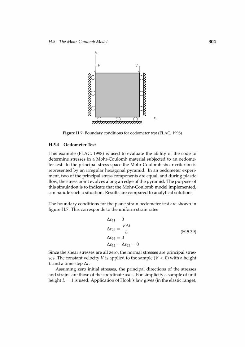
H.5. The Mohr-Coulomb Model 304
x1
x2
V V
Figure H.7: Boundary conditions for oedometer test (FLAC, 1998)
H.5.4 Oedometer Test
This example (FLAC, 1998) is used to evaluate the ability of the code todetermine stresses in a Mohr-Coulomb material subjected to an oedome-ter test. In the principal stress space the Mohr-Coulomb shear criterion isrepresented by an irregular hexagonal pyramid. In an oedometer experi-ment, two of the principal stress components are equal, and during plasticflow, the stress point evolves along an edge of the pyramid. The purpose ofthis simulation is to indicate that the Mohr-Coulomb model implemented,can handle such a situation. Results are compared to analytical solutions.
The boundary conditions for the plane strain oedometer test are shown infigure H.7. This corresponds to the uniform strain rates
∆ε11 = 0
∆ε22 =V∆t
L∆ε33 = 0∆ε12 = ∆ε21 = 0
(H.5.39)
Since the shear stresses are all zero, the normal stresses are principal stres-ses. The constant velocity V is applied to the sample (V < 0) with a heightL and a time step ∆t.
Assuming zero initial stresses, the principal directions of the stressesand strains are those of the coordinate axes. For simplicity a sample of unitheight L = 1 is used. Application of Hook’s law gives (in the elastic range),

H.5. The Mohr-Coulomb Model 305
using ε22 = Vt at time t
σ11 = α2Vtσ22 = α1Vtσ33 = α2Vt = σ11
(H.5.40)
The Mohr-Coulomb yield functions are given by equation H.5.3
f 1 = σ22 − σ11Nφ + 2c√
Nφ
f 2 = σ22 − σ33Nφ + 2c√
Nφ
(H.5.41)
At the onset of yield f 1 = f 2 = 0. Using equation H.5.40 and equa-tion H.5.41, we find
t =2c√
Nφ
−V(α1 − α2Nφ)(H.5.42)
Yielding only takes place provided that α1− α2Nφ > 0. During plastic flow,the strain increments are composed of elastic and plastic parts
∆ε11 = ∆εe11 + ∆ε
p11
∆ε22 = ∆εe22 + ∆ε
p22
∆ε33 = ∆εe33 + ∆ε
p33
(H.5.43)
Using the boundary conditions in equation H.5.39 it follows that
∆εe11 = −∆ε
p11
∆εe22 = V∆t− ∆ε
p22
∆εe33 = −∆ε
p33
(H.5.44)
The flow rule for plastic flow along the edge of the Mohr-Coulomb criterioncorresponding to σ11 = σ33 has the form (FLAC, 1998)
∆εp11 = λ1
∂g1
∂σ11+ λ2
∂g2
∂σ11
∆εp22 = λ1
∂g1
∂σ22+ λ2
∂g2
∂σ22
∆εp33 = λ1
∂g1
∂σ33+ λ2
∂g2
∂σ33
(H.5.45)
where g1 and g2 are the potential functions corresponding to f 1 and f 2,equation H.5.8
g1 = σ22 − σ11Nψ
g2 = σ22 − σ33Nψ
(H.5.46)

H.5. The Mohr-Coulomb Model 306
After partial differentiation and substitution into equation H.5.45, we find
∆εp11 = −λ1Nψ
∆εp22 = λ1 + λ2
∆εp33 = −λ2Nψ
(H.5.47)
In further considering that, by symmetry, λ1 = λ2, we obtain
∆εp11 = −λ1Nψ
∆εp22 = 2λ1
∆εp33 = −λ2Nψ
(H.5.48)
The stress increments (Hook’s law) are given by
∆σ11 = α1∆εe11 + α2(∆εe
22 + ∆εe11)
∆σ22 = α1∆εe22 + 2α2∆εe
11
∆σ33 = ∆σ11
(H.5.49)
where ∆εe11 = ∆εe
33. Substitution of equation H.5.44 in equation H.5.49 andusing equation H.5.48 yields
∆σ11 = α1λ1Nψ + α2(V∆t− 2λ1 + λ1Nψ)∆σ22 = α1(V∆t− 2λ1) + 2α2λ1Nψ
∆σ33 = ∆σ11
(H.5.50)
The plastic multiplier λ1 may now be determined by expressing the condi-tion that, during plastic flow, ∆ f 1 = 0. Using equation H.5.41, this condi-tion takes the form
∆σ22 − ∆σ11Nφ = 0 (H.5.51)
Substitution of equation H.5.50 in equation H.5.51 yields, after some mani-pulations
λ1 = Vλ∆t (H.5.52)
where
λ =α1 − α2Nφ
(α1 + α2)NφNψ − 2α2(Nφ + Nψ) + 2α1(H.5.53)
This analytical (exact) solution is compared to a numeric experiment usingone element with 9 particles (3x3) in Chapter 4.
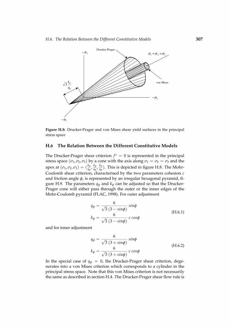
H.6. The Relation Between the Different Constitutive Models 307
1σ−
2σ−
3σ−321 σσσ ==
Drucker-Prager
von Mises
φ
φ
q
k3
Figure H.8: Drucker-Prager and von Mises shear yield surfaces in the principalstress space
H.6 The Relation Between the Different Constitutive Models
The Drucker-Prager shear criterion f s = 0 is represented in the principalstress space (σ1, σ2, σ3) by a cone with the axis along σ1 = σ2 = σ3 and theapex at (σ1, σ2, σ3) = ( kφ
qφ, kφ
qφ, kφ
qφ). This is depicted in figure H.8. The Mohr-
Coulomb shear criterion, characterised by the two parameters cohesion cand friction angle φ, is represented by an irregular hexagonal pyramid, fi-gure H.9. The parameters qφ and kφ can be adjusted so that the Drucker-Prager cone will either pass through the outer or the inner edges of theMohr-Coulomb pyramid (FLAC, 1998). For outer adjustment
qφ =6√
3 (3− sinφ)sinφ
kφ =6√
3 (3− sinφ)c cosφ
(H.6.1)
and for inner adjustment
qφ =6√
3 (3 + sinφ)sinφ
kφ =6√
3 (3 + sinφ)c cosφ
(H.6.2)
In the special case of qφ = 0, the Drucker-Prager shear criterion, dege-nerates into a von Mises criterion which corresponds to a cylinder in theprincipal stress space. Note that this von Mises criterion is not necessarilythe same as described in section H.4. The Drucker-Prager shear flow rule is

H.6. The Relation Between the Different Constitutive Models 308
1σ−
2σ−
3σ−
321 σσσ ==
Tresca
Mohr-Coulomb
φtan3
c
Figure H.9: Mohr-Coulomb and Tresca shear yield surfaces in the principal stressspace
non-associated, while the von Mises flow rule employed here has an asso-ciated flow rule. The Drucker-Prager model, however, reduces to the vonMises model described in section H.4 if the following parameter values areused.
qφ = 0
kφ =σy√
3
σt =kφ
qφ= ∞
qψ = 0
(H.6.3)
where σy is the yield stress in simple tension and with qψ = 0, the shear flowrule is associated. With σt = ∞, the tensile yield mode is not employed.
The Tresca criterion is a special case of the Mohr-Coulomb criterion forwhich φ = 0. It is represented by a regular hexagonal prism. The von Misescylinder circumscribes the Tresca prism for
qφ = 0
kφ =2√3
c(H.6.4)

Appendix I
Cosserat Continuum ConstitutiveModels and Implementation
I.1 Introduction
Constitutive models for a Cosserat continuum are presented. This includeselasticity and elasto-plastic models.
I.2 Cosserat Plane Strain Elasticity
This section closely follows the work of de Borst (1991) and de Borst (1993).In this model, two-dimensional, planar motion is considered. In this case,each material point has two translational degrees-of-freedom, namely u1and u2 and a rotational degree-of-freedom wc
3, the rotation axis of which isorthogonal to the x1x2-plane.
The single, tensorial deformation measure is given by (Appendix C),equation C.3.7
λij = ui,j + ε ijkwck (I.2.1)
or for planar deformation
λ =
λ11 λ12 λ13λ21 λ22 λ23λ31 λ32 λ33
=
u1,1 (u1,2 + wc3) 0
(u2,1 − wc3) u2,2 0
0 0 u3,3
The micro-curvature is given by
κij = wci,j (I.2.2)
or for planar deformation
κ =
0 0 00 0 0
κ31 κ32 0
In formulating elasto-plasticity, it is useful to rather use generalised curva-tures κ31l and κ32l, where l is a material parameter with the dimension oflength. It is this parameter which effectively sets the internal length scalein the continuum, and therefore has the role of a “characteristic length”.
309

I.2. Cosserat Plane Strain Elasticity 310
The strain components can be assembled in a vector (for the two-dimensionalcase)
εc = [λ11 λ22 λ33 λ12 λ21 κ31l κ32l]T (I.2.3)
Note that the normal strain in the x3-direction, λ33 = u3,3, has also beenincluded in the strain vector. This has been done because, although thisstrain component remains zero under plane strain conditions during theentire loading process, this is not necessarily the case for the elastic andplastic contributions of this strain component. Also note that by multiply-ing the micro-curvatures by the length parameter l, all components of thestrain vector εc have the same dimension.
While the strain vector εc is comprised of seven components for planardeformations, so is the stress vector σ c. The couple-stresses µij are conju-gate to the micro-curvatures κij. Dividing the couple-stresses by the lengthparameter l, we obtain a stress vector σc in which all the entries have thesame dimension.
σ c =[σ11 σ22 σ33 σ12 σ21
µ31
lµ32
l
]T(I.2.4)
Assuming that the elastic strain vector is linearly related to the stress vector,the following equation can be written
σ c = Deεce (I.2.5)
where De is the stiffness matrix containing the elastic moduli
De =
2Gc1 2Gc2 2Gc2 0 0 0 02Gc2 2Gc1 2Gc2 0 0 0 02Gc2 2Gc2 2Gc1 0 0 0 0
0 0 0 (G + Gc) (G− Gc) 0 00 0 0 (G− Gc) (G + Gc) 0 00 0 0 0 0 2G 00 0 0 0 0 0 2G
(I.2.6)
with c1 = 1−ν1−2ν and c2 = ν
1−2ν , G is the shear modulus and v Poisson’sratio. Gc is an additional material constant, completing the four materialconstants that are needed to describe the elastic behaviour of an isotropicCosserat continuum under planar deformations. The coefficient 2 has beenintroduced in terms De
66 and De77 in order to arrive at a convenient form of
the elasto-plastic constitutive equations. The total (bending) stiffness thatsets the relation between the micro-curvatures and the couple stresses isbasically determined by the value of the internal length scale l.

I.2. Cosserat Plane Strain Elasticity 311
Expanding equation I.2.5, the terms become
σc11 = 2G
(1− v
1− 2v
)λ11 + 2G
(v
1− 2v
)λ22 + 2G
(v
1− 2v
)λ33
= 2G(
1− v1− 2v
)ε11 + 2G
(v
1− 2v
)ε22 + 2G
(v
1− 2v
)ε33
(I.2.7)
σc22 = 2G
(v
1− 2v
)λ11 + 2G
(1− v1− 2v
)λ22 + 2G
(v
1− 2v
)λ33
= 2G(
v1− 2v
)ε11 + 2G
(1− v1− 2v
)ε22 + 2G
(v
1− 2v
)ε33
(I.2.8)
σc33 = 2G
(v
1− 2v
)λ11 + 2G
(v
1− 2v
)λ22 + 2G
(1− v1− 2v
)λ33
= 2G(
v1− 2v
)ε11 + 2G
(v
1− 2v
)ε22 + 2G
(1− v1− 2v
)ε33
(I.2.9)
It can be seen that the expressions for normal stress are the same as in thecase of the classical non-polar continuum. The expressions for the shearstresses, however, are different.
σc12 = (G + Gc) λ12 + (G− Gc) λ21
= (G + Gc)(
∂u1
∂x2+ wc
3
)+ (G− Gc)
(∂u2
∂x1− wc
3
)= G
(∂u1
∂x2+
∂u2
∂x1
)+ 2Gc
[12
(∂u1
∂x2− ∂u2
∂x1
)+ wc
z
]= Gε12 + 2Gc
[12
(∂u1
∂x2− ∂u2
∂x1
)+ wc
3
]= nonpolar + polar
(I.2.10)
σc21 = (G− Gc) λ12 + (G + Gc) λ21
= G(
∂u1
∂x2+
∂u2
∂x1
)+ 2Gc
[12
(∂u2
∂x1− ∂u1
∂x2
)− wc
3
]= Gε21 + 2Gc
[12
(∂u2
∂x1− ∂u1
∂x2
)− wc
3
]= nonpolar + polar
(I.2.11)
The curvature equations are
µ31
l= 2Gκ31l → µ31 = 2Gκ31l2 (I.2.12)

I.3. Cosserat von Mises Elasto-Plasticity 312
µ32
l= 2Gκ32l → µ32 = 2Gκ32l2 (I.2.13)
Thus, for Cosserat elasticity, the following material constants must be known:
1. Shear modulus, G
2. Poisson’s ration, v
3. Characteristic length, l
4. Cosserat shear modulus, Gc
I.3 Cosserat von Mises Elasto-Plasticity
This section closely follows the work of de Borst (1991). In this treatment arestriction of J2-flow theory is used. The yield function f can be written as
f = (3J2)12 − σ (γ) (I.3.1)
with σ the yield stress which is a function of the hardening parameter γ. J2is the second invariant of the deviatoric stresses, and for a polar-continuumit can be generalised as (Muhlhaus and Vardoulakis, 1987).
J2 = a1sijsij + a2sijsji +a3µijµij
l2 (I.3.2)
sij is the deviatoric stress tensor, µijis the couple-stress tensor and a1, a2and a3 are material parameters. In the absence of couple stresses, µij = 0,sij = sji and equation I.3.2 reduces to
J2 = (a1 + a2) sijsij (I.3.3)
which implies that the constraint
a1 + a2 = 12 (I.3.4)
must be enforced so as to achieve that the classical expression for J2 beretrieved properly. For the case of planar deformations, J2 can be written inthe following form
J2 = 12
[s2
11 + s222 + s2
33]+ a1σ2
12 + 2a2σ12σ21 + a1σ221 + a3
[(µ31
l
)2+(µ32
l
)2]
(I.3.5)Muhlhaus & Vardoulakis (1987) proposed values of a1 = 3
4 , a2 = − 14 and
a3 = 18 . de Borst (1991) used a1 = 1
4 , a2 = 14 and a3 = 1
2 , since these

I.3. Cosserat von Mises Elasto-Plasticity 313
values give rise to a particularly simple numerical algorithm. Using matrixnotation, equation I.3.5 can be written as
J2 = 12 σcP σ c (I.3.6)
where P (for planar deformation) is given by
P =
23 − 1
3 − 13 0 0 0 0
− 13
23 − 1
3 0 0 0 0− 1
3 − 13
23 0 0 0 0
0 0 0 2a1 2a2 0 00 0 0 2a2 2a1 0 00 0 0 0 0 2a3 00 0 0 0 0 0 2a3
(I.3.7)
Substituting equation I.3.6 into equation I.3.1 leads to
f =( 3
2 σcP σ c) 12 − σ (γ) (I.3.8)
An associated flow rule is now obtained in a fashion identical to that in aclassical non-polar continuum.
εcp = λ∂ f
∂σ c (I.3.9)
Using equation I.3.8 and the fact that f = 0 during plastic flow, this beco-mes
εcp = λ3P σ c
2( 3
2 σcP σ c) 12
=3λ
2σ (γ)P σ c (I.3.10)
λ is the plastic multiplier which, in analogy with classical plasticity, is de-termined from the consistency condition f = 0.
The hardening parameter γ for Cosserat J2-flow theory remains to beidentified. The conventional strain-hardening hypothesis
γ =[
23 ep
ij epij
] 12 (I.3.11)
with epij the plastic deviatoric strain-rate tensor. For uniaxial stress condi-
tions γ reduces to the uniaxial plastic strain rate, γ = εp11. Since there are
no couple-stress effects in pure uniaxial loading, we require that any modi-fication to equation I.3.11 for Cosserat media does not affect the result forpure uniaxial loading. A possible generalisation is to postulate that (equa-tion I.3.2)
γ =[b1ep
ij epij + b2ep
ij epji + b3κ
pijκ
pijl
2] 1
2 (I.3.12)
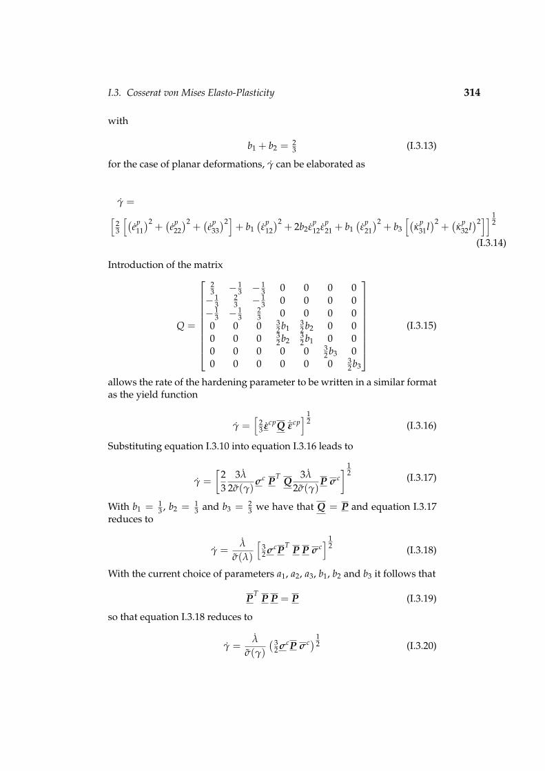
I.3. Cosserat von Mises Elasto-Plasticity 314
with
b1 + b2 = 23 (I.3.13)
for the case of planar deformations, γ can be elaborated as
γ =[23
[(ep
11
)2 +(ep
22
)2 +(ep
33
)2]+ b1
(ε
p12
)2 + 2b2 εp12 ε
p21 + b1
(ε
p21
)2 + b3
[(κ
p31l)2 +
(κ
p32l)2]] 1
2
(I.3.14)
Introduction of the matrix
Q =
23 − 1
3 − 13 0 0 0 0
− 13
23 − 1
3 0 0 0 0− 1
3 − 13
23 0 0 0 0
0 0 0 32 b1
32 b2 0 0
0 0 0 32 b2
32 b1 0 0
0 0 0 0 0 32 b3 0
0 0 0 0 0 0 32 b3
(I.3.15)
allows the rate of the hardening parameter to be written in a similar formatas the yield function
γ =[
23 εcpQ εcp
] 12 (I.3.16)
Substituting equation I.3.10 into equation I.3.16 leads to
γ =[
23
3λ
2σ(γ)σc PT Q
3λ
2σ(γ)P σ c
] 12 (I.3.17)
With b1 = 13 , b2 = 1
3 and b3 = 23 we have that Q = P and equation I.3.17
reduces to
γ =λ
σ(λ)
[32 σcPT P P σ c
] 12 (I.3.18)
With the current choice of parameters a1, a2, a3, b1, b2 and b3 it follows that
PT P P = P (I.3.19)
so that equation I.3.18 reduces to
γ =λ
σ(γ)( 3
2 σcP σ c) 12 (I.3.20)

I.3. Cosserat von Mises Elasto-Plasticity 315
In the plastic state f = 0 and from equation I.3.8 it follows that
f =( 3
2 σcP σ c) 12 − σ(γ) = 0 →
( 32 σcP σ c) 1
2 = σ(γ) (I.3.21)
Substituting this into equation I.3.20 leads to
γ = λ (I.3.22)
which is the same format as obtained in classical J2-flow theory.
I.3.1 Algorithm
In this section an algorithm that determines the stress increment in a finiteloading step is given. A one-step return-mapping algorithm in which thegradient is evaluated at the trail stress state is used. As in classical plasticitythe algorithm starts by computing a trail stress state
σtc = σ0
c + De∆εc (I.3.23)
The trail stress state is checked whether plasticity will indeed occur for thisintegration point within this loading step. σ0
c is the stress at the beginningof the loading step. If plasticity indeed occurs, i.e. if f (σt
c, γ0) > 0, acorrection for plastic flow is applied.
The yield function f (σ c, γ) = 0, is written as a truncated Taylor series(Gerald and Wheatley, 1999) around (σt
c, γ0).
f (σ c, γ) = f (σtc, γ0) +
(∂ f
∂σ c
)T
(σ c − σtc) +
∂ f∂γ
(γ− γ0) +(∂2 f∂σ c2
)T (σ c − σtc)2
2!+
∂2 f∂γ2
(γ− γ0)2
2!+ · · · = 0 (I.3.24)
Evaluating this series at ( cσn, γn) where n denotes the value of a quantityafter correction for plastic flow and noting that (figure I.1),
( cσn − σtc) = De ∆εcp = −De ∆λ
∂ f∂σ c (I.3.25)
equation I.3.24 can be written as
f (σtc, γ0)− ∆λ
(∂ f
∂σ c
)T
De ∂ f∂σ c + ∆γ
∂ f∂γ
+
12
∆λ2(
∂ f∂σ c
)T
De ∂2 f∂σ c2 De ∂ f
∂σ c +12
∆γ2 ∂2 f∂γ2 + · · · = 0 (I.3.26)

I.3. Cosserat von Mises Elasto-Plasticity 316
Introduction of the hardening modulus in a fashion identical to classicalplasticity
h (γ) =∂σ
∂γ(I.3.27)
and use of the finite counterpart of equation I.3.22 permit equation I.3.26 tobe written as
f (σtc, γ0)− ∆λ
(h +
(∂ f
∂σ c
)T
De ∂ f∂σ c
)
+12
∆λ2
(∂2 f∂γ2 +
(∂ f
∂σ c
)T
De ∂2 f∂σ c2 De ∂ f
∂σ c
)+ · · · = 0 (I.3.28)
where∂ f∂γ
=∂ f∂σ
∂σ
∂γ=
∂σ
∂γ(I.3.29)
For the present choice of a1, a2, a3, b1, b2 and b3 and restricting the treat-ment to linear hardening or softening, h (γ) = h, second and higher-ordercontributions in ∆λ vanish (de Borst, 1991), so that we obtain an explicitexpression for the plastic multiplier ∆λ
∆λ =f (σt
c, γ0)
h + ∂ f T
∂σ c De ∂ f∂σ c
(I.3.30)
Note that in this explicit formulation the gradient of the yield function ∂ f∂σ c
is evaluated for σ c = σtc.
With equation I.3.30 for the magnitude of the plastic strain incrementthe algorithm for elasto-plasticity in a Cosserat continuum can be formu-lated in complete analogy to a conventional plasticity model. The strainincrement is decomposed in an elastic part εce and a plastic part εcp.
∆εc = ∆εce + ∆εcp (I.3.31)
Similar to classical plasticity, a bijective relationship is assumed betweenthe elastic strain increment and the stress increment, figure I.1.
∆σ c = De∆εce (I.3.32)
The new stress state, i.e. the stress at the end of the increment, is the sumof the stress at the beginning of the step and the stress increment.
cσn = σ0c + ∆σ c (I.3.33)

I.4. Generalisation of J2-flow Theory 317
σ0
σn
σt
ε0 εn
σ
ε
∆ε
∆σ
∆ε p∆ε eE
1
Figure I.1: One-dimensional representation of elasto-plastic relation
Substituting equation I.3.32 into equation I.3.33 leads to
cσn = σ0c + De∆εce (I.3.34)
where σ0c is known, but ∆εce still unknown. Using equation I.3.31, equa-
tion I.3.34 can be written as
cσn = σ0c + De (∆εc − ∆εcp)
= σ0c + De∆εc − De∆εcp
= σtc − De∆εcp
(I.3.35)
where σtc is the trial stress by assuming the total strain increment to be
elastic. Using equation I.3.10 for the plastic strain increment, the new stressstate can be written as
cσn = σtc − 3λ
2σ(γ)DeP σt
c (I.3.36)
where the plastic increment is given by equation I.3.30. Note that by vir-tue of the vanishing of the second and higher-order contributions in ∆λin equation I.3.28 the algorithm as laid down in equation I.3.36 provides arigorous return to the yield surface.
I.4 Generalisation of J2-flow Theory
A pressure dependent J2-flow theory is proposed by de Borst (1993) for usewithin the framework of the Cosserat continuum.
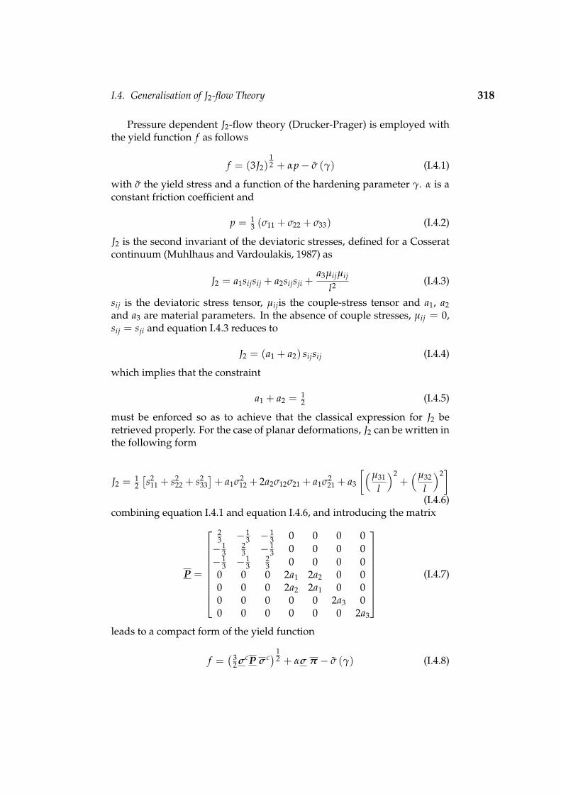
I.4. Generalisation of J2-flow Theory 318
Pressure dependent J2-flow theory (Drucker-Prager) is employed withthe yield function f as follows
f = (3J2)12 + αp− σ (γ) (I.4.1)
with σ the yield stress and a function of the hardening parameter γ. α is aconstant friction coefficient and
p = 13 (σ11 + σ22 + σ33) (I.4.2)
J2 is the second invariant of the deviatoric stresses, defined for a Cosseratcontinuum (Muhlhaus and Vardoulakis, 1987) as
J2 = a1sijsij + a2sijsji +a3µijµij
l2 (I.4.3)
sij is the deviatoric stress tensor, µijis the couple-stress tensor and a1, a2and a3 are material parameters. In the absence of couple stresses, µij = 0,sij = sji and equation I.4.3 reduces to
J2 = (a1 + a2) sijsij (I.4.4)
which implies that the constraint
a1 + a2 = 12 (I.4.5)
must be enforced so as to achieve that the classical expression for J2 beretrieved properly. For the case of planar deformations, J2 can be written inthe following form
J2 = 12
[s2
11 + s222 + s2
33]+ a1σ2
12 + 2a2σ12σ21 + a1σ221 + a3
[(µ31
l
)2+(µ32
l
)2]
(I.4.6)combining equation I.4.1 and equation I.4.6, and introducing the matrix
P =
23 − 1
3 − 13 0 0 0 0
− 13
23 − 1
3 0 0 0 0− 1
3 − 13
23 0 0 0 0
0 0 0 2a1 2a2 0 00 0 0 2a2 2a1 0 00 0 0 0 0 2a3 00 0 0 0 0 0 2a3
(I.4.7)
leads to a compact form of the yield function
f =( 3
2 σcP σ c) 12 + ασ π − σ (γ) (I.4.8)

I.4. Generalisation of J2-flow Theory 319
with π =[ 1
313
13 0 0 0
]A non-associated flow rule is obtained in an identi-
cal fashion to that in a nonpolar continuum.
εcp = λ∂g
∂σ c (I.4.9)
where
g =( 3
2 σcP σ c) 12 + β σ π − σ (γ) (I.4.10)
is the plastic potential function and β is a dilatancy factor. Equation I.4.9becomes
εcp = λ3P σ c
2( 3
2 σcP σ c) 12
+ β π (I.4.11)
λ is the plastic multiplier which, in analogy with classical plasticity, is de-termined from the consistency condition f = 0.
It now remains to identify the plastic strain measure γ (hardening pa-rameter) for a J2-flow theory in a Cosserat continuum. For this purpose,recall the conventional strain-hardening hypothesis
γ =[
23 ep
ij epij
] 12 (I.4.12)
with epij the plastic deviatoric strain-rate tensor. For uniaxial stress conditi-
ons γ reduces to the uniaxial plastic strain rate, γ = εp11. Since there are no
couple-stress effects in pure uniaxial loading, we require that any modifica-tion to equation I.4.12 for Cosserat media does not affect the result for pureuniaxial loading. A possible generalisation is to postulate that, analogousto equation I.4.3
γ =[b1ep
ij epij + b2ep
ij epji + b3κ
pijκ
pijl
2] 1
2 (I.4.13)
with
b1 + b2 = 23 (I.4.14)
for the case of planar deformations, γ can be elaborated as
γ =[23
[(ep
11
)2 +(ep
22
)2 +(ep
33
)2]+ b1
(ε
p12
)2 + 2b2 εp12 ε
p21 + b1
(ε
p21
)2 + b3
[(κ
p31l)2 +
(κ
p32l)2]] 1
2
(I.4.15)

I.4. Generalisation of J2-flow Theory 320
Introduction of the matrix
Q =
23 − 1
3 − 13 0 0 0 0
− 13
23 − 1
3 0 0 0 0− 1
3 − 13
23 0 0 0 0
0 0 0 32 b1
32 b2 0 0
0 0 0 32 b2
32 b1 0 0
0 0 0 0 0 32 b3 0
0 0 0 0 0 0 32 b3
(I.4.16)
allows the rate of the hardening parameter to be written in a similar formatas the yield function
γ =[
23 εcpQ εcp
] 12 (I.4.17)
Substitution of equation I.4.11 into equation I.4.17 and noting that Q π = 0,it follows
γ = λ
[σ P Q P σ
σ P σ
] 12
(I.4.18)
if the parameters a1, a2, a3, b1, b2 and b3 are chosen such that
P Q P = P (I.4.19)
equation I.4.18 reduces to exactly the same format as obtained in standardJ2-flow theory:
γ = λ (I.4.20)
I.4.1 A Return-mapping Algorithm
The trial stress state σtc is defined as
σtc = σ0
c + De∆εc (I.4.21)
where σ0c is the stress at the beginning of the loading step. It has been
shown by (de Borst, 1991) (section I.3) that for certain classes of materialparameters, there exists a set of values a1, a2, a3, b1, b2 and b3, which ensu-res a return to the yield surface in a single iteration. These advantageousproperties are obtained for a1 = a2 = 1
4 , a3 = 12 , b1 = b2 = 1
3 and b3 = 23 .
This set of constants is referred to as the “standard” set.When these conditions are not satisfied, an Euler backward algorithm
can be employed. In this algorithm, the total strain increment in a finite loa-

I.4. Generalisation of J2-flow Theory 321
ding step ∆εc is decomposed into an elastic contribution ∆εce and a plasticcontribution ∆εcp.
∆εc = ∆εce + ∆εcp (I.4.22)
Between the stress increment ∆σ c and the elastic strain increment ∆εc, wehave the bijective relationship (figure I.1)
∆σ c = De∆εce (I.4.23)
The new stress state, i.e. the stress at the end of the increment, is the sumof the stress at the beginning of the step and the stress increment.
cσn = σ0c + ∆σ c (I.4.24)
Substituting equation I.4.23 into equation I.4.24 leads to
cσn = σ0c + De∆εce (I.4.25)
where σ0c is known, but ∆εce still unknown. Using equation I.4.22, equa-
tion I.4.25 can be written as
cσn = σ0c + De (∆εc − ∆εcp)
= σ0c + De∆εc − De∆εcp
= σtc − De∆εcp
(I.4.26)
where σtc is the trial stress by assuming the total strain increment to be ela-
stic. Furthermore„ the expression for the plastic strain rate, equation I.4.11,is integrated using a single-point Euler backward rule (Gerald and Whea-tley, 1999).
∆εcp = ∆λ
3P cσn
2( 3
2 σcnP cσn
) 12
+ β π
(I.4.27)
where the subscript n refers to the value at the end of the loading step.Substitution of equation I.4.27 into equation I.4.26 leads to
cσn = σtc − ∆λ
3 De P cσn
2( 3
2 σcnP cσn
) 12
+ β Deπ
(I.4.28)
The condition that at the end of the loading step the yield condition mustbe satisfied, f ( cσn, γn), is used. Equation I.4.28 transforms into
cσn = σtc − ∆λ
[3 De P cσn
2 [σ(γn)− α π cσn]+ β De
π
](I.4.29)

I.5. Cosserat Drucker-Prager Elasto-Plasticity 322
A complication now arises, since we wish to express cσn as a function of σtc
and ∆λ, while in equation I.4.29 cσn also occurs in the denominator of thesecond term on the right-hand side. To overcome this problem, we expressπ cσn as a function of π σt
c and ∆λ by pre-multiplying equation I.4.29 bythe projection vector π. Since π DeP = 0 , this gives
π cσn = π σtc − ∆λβ π De
π
= π σtc − ∆λβ K
(I.4.30)
Substitution of this identity into equation I.4.29 results in the desired for-mulation.
cσn = σtc − ∆λ
[3 De P cσn
2 [σ(γn)− α (π σtc − ∆λβ K)]
+ β Deπ
]= A−1
(σt
c − ∆λβ Deπ) (I.4.31)
where
A = I +3 ∆λ De P
2 [σ(γn) + ∆λ α β K− α π σtc)
(I.4.32)
and I is a 7 × 7 matrix with ones on the diagonal and zeros everywhereelse. Substitution of equation I.4.31 into the yield condition f ( cσn, γn) = 0results in a non-linear equation in ∆γ
f (∆λ) =[
32
(σt
c − ∆λβ Deπ)T (
A−1)T
P(
A−1) (
σtc − ∆λβ De
π)] 1
2
+ α π(
A−1) (
σtc − ∆λβ De
π)− σ(γn) = 0 (I.4.33)
This equation can be solved using the Regula-Falsi method (Phillips et al.,1998). Convergence is achieved within 4-5 iterations (de Borst, 1993).
I.5 Cosserat Drucker-Prager Elasto-Plasticity
This model is similar to the model described in the previous section, butwith some small changes in implementation. The model was proposedby Muhlhaus (1987). The description given here closely follows that ofTejchman (1997).
The yield function f is given by
f = q + α(γp)p− c (I.5.1)

I.5. Cosserat Drucker-Prager Elasto-Plasticity 323
and the potential function g by
g = q + β(γp)p (I.5.2)
where
q =√
J2 (I.5.3)
and
p =12
(σ11 + σ22 + σ33) (I.5.4)
The second invariant of the deviatoric stress tensor J2 is given by equa-tion I.3.2.
J2 = a1sijsij + a2sijsji +a3µijµij
l2 (I.5.5)
sij is the deviatoric stress tensor, α is a friction factor, β a dilatancy factor,c is cohesion and a1, a2 and a3 are material parameters as described in theprevious two sections with the constraint that a1 + a2 = 1
2 . The plastic shearstrain rate γp, is again given by equation I.3.12
γp =[b1ep
ij epij + b2ep
ij epji + b3κ
pijκ
pijl
2] 1
2 (I.5.6)
Muhlhaus (1987) derived, on macroscopic level, and expression for γ bytaking into account slip and rotation in a random assembly of circular rodswith a fixed diameter,
γp =[3ep
ij epij − ep
ij epji + κ
pijκ
pijl
2] 1
2 (I.5.7)
i.e. b1 = 3, b2 = −1 and b3 = 1. Further, by assuming that q and γp arework-conjugate (Muhlhaus, 1987)
qγp = sij eij + µiκi (I.5.8)
it can be shown that a1 = 38 , a2 = 1
8 and a3 = 1. This complies to theconstraint that a1 + a2 = 1
2 . From micromechanical considerations it canalso be shown that (Muhlhaus and Vardoulakis, 1987)
Gc =G
2 (a1 − a2)(I.5.9)
The stresses and strains are assembled in vectors as shown by equation I.2.3and I.2.4
εc = [λ11 λ22 λ33 λ12 λ21 κ31l κ32l]
σc =[σ11 σ22 σ33 σ12 σ21
µ31
lµ32
l
] (I.5.10)

I.5. Cosserat Drucker-Prager Elasto-Plasticity 324
A trial stress method (linearised expansion of the yield condition aboutthe trial stress point) using an elastic predictor and a plastic corrector withradial return mapping is used (Tejchman, 1997). According to this algo-rithm, the plastic multiplier ∆λ is given by
∆λ =f (σt
c, γ0)
h + ∂ f T
∂σ c De ∂g∂σ c
(I.5.11)
where σtc is the trial stress state, calculated by assuming the total strain
increment to be elastic, equation I.3.23, and h is the hardening modulus.Note that this expression is similar to what is given by equation I.3.30. Thegradients ∂ f
∂σ c and ∂g∂σ c are evaluated at the trial stress point. Similar to equa-
tion I.3.36, the new stress state can be calculated using
cσn = σtc − ∆λDe ∂g
∂σ c (I.5.12)
This new stress state cσn would not necessarily be on the yield functionf = 0. Therefor, the calculations are continued until the stress state lieson the yield surface. Iterations are used where the newest stress state issubstituted for σt
c in equation I.5.12 and f , ∂ f∂σ c , ∂g
∂σ c , α, β and h are computedin each iteration using the newest stress state. No more than two or threeiterations were needed to satisfy the condition f
q ≤ 10−6.The gradients are calculated as follows (Tejchman, 1997)
∂ f∂σ c =
1q
s112
s222
s332
3s128 + s21
83s21
8 + s128
µ31l2
µ32l2
+
12
αα00000
(I.5.13)
∂g∂σ c =
1q
s112
s222
s332
3s128 + s21
83s21
8 + s128
µ31l2
µ32l2
+
12
ββ00000
(I.5.14)
and also
∂ f T
∂σ c De ∂g∂σ c = G + αβB (I.5.15)
where B = G1−2ν and it has been assumed that a1 = 3
8 , a2 = 18 and a3 = 1
References
Adhikary, D., Muhlhaus, H.-B. and Dyskin, A. (1999). Modelling the largedeformations in stratified media - the cosserat continuum approach. Me-chanics of Cohesive-Frictional Materials, vol. 4, pp. 195–213. (Cited on pa-ges 7 and 9.)
Albert, R., Pfeifer, M., Shiffer, P. and Barabasi, A. (1998). Drag force in agranular medium. Www.nd.edu. (Cited on page 95.)
Bagster, D. and Bridgwater, J. (1967). The measurement of the force neededto move blades through a bed of cohesionless granules. Powder Techno-logy. (Cited on page 95.)
Bardenhagen, S.G., Brackbill, J.U. and Sulsky, D.L. (2000). The material-point method for granular materials. Computational Methods in AppliedMechanics and Engineering, vol. 187, pp. 529–541. (Cited on pages 11, 28,39, 270, and 276.)
Belytschko, T., Krongauz, Y., Organ, D., Flemming, M. and Krysl, P. (1996).Meshless methods: An overview and recent developments. Tech. Rep., ,Northmestern University. (Cited on pages 8 and 9.)
Belytschko, T., Lu, Y.Y. and Gu, L. (1994). Element free galerkin methods.Int. Journal. Numer. Methods. Eng., vol. 37, pp. 229–256. (Cited on page 10.)
Benham, P., Crawford, R. and Armstrong, C. (1996). Mechanics of Eninee-ring Materials. 2nd edn. Addison Wesley Longman Limited. (Cited onpage 301.)
Benson, D. (1992). Computational methods in lagrangian and eulerian hy-drocodes. Computer Methods in Applied Mechanics and Engineering, vol. 99,pp. 235–394. (Cited on page 10.)
Beverloo, W., Leniger, H. and Van de Velde, J. (1961). The flow of granularsolids through orifices. Chemical Engineering Science, vol. 15, pp. 260–269.(Cited on page 58.)
Blazynski, T. (1983). Applied Elasto-Plasticity of Solids. MacMillan Press,London, England. (Cited on page 285.)
Bohatier, C. and Nouguier, C. (1999). Numerical Modelling of Large Deforma-tions in Soils: Continuum or Granular Medium. Energy Sources TechnologyConference & Exhibition, ETCE99-6713, ASME. (Cited on pages 3, 9,and 14.)
325

References 326
Bohatier, C. and Nouguier, C. (2000). Dynamic soil-tool interaction forcesand flow state. In: International Conference on Applied Mechanics, pp. 294–299. Durban, South Africa. (Cited on pages 3 and 95.)
Boresi, A. and Chong, K. (2000). Elasticity in Engineering Mechanics. 2ndedn. John Wiley & Sons, Inc., New York. (Cited on pages 4 and 212.)
Brackbill, J.U., Kothe, D.B. and Ruppel, H.M. (1988). Flip: A low-dissipation, particle-in-cell method for fluid flow. Comput. Phys. Commun,vol. 48, pp. 25–38. (Cited on pages 20 and 261.)
Brackbill, J.U. and Ruppel, H.M. (1988). Flip: A method for adaptivelyzoned, particle-in-cell calculations in two dimensions. J. Comput. Phys.,vol. 65, pp. 314–343. (Cited on pages 10 and 261.)
Brown, C., Lahlouh, E. and Rotter, J. (2000). Experiments on a square plan-form steel silo. Chemical Engineering Science, vol. 55, pp. 4399–4413. (Citedon pages 131 and 133.)
Burgess, D., Sulsky, D. and Brackbill, J.U. (1992). Mass matrix formulationof the FLIP particle-in-cell method. J. Comput. Phys., vol. 103, pp. 1–15.(Cited on pages 11, 19, 260, and 261.)
Cerrolaza, M., Sulem, J. and Elbied, A. (1999). A cosserat non-linear finiteelement analysis software for blocky structures. Advances in EngineeringSoftware, vol. 30, pp. 69–83. (Cited on page 7.)
Chen, Z., Hu, W., Shen, L., Xin, X. and Brannon, R. (2002). An evaluationof the MPM for simulating dynamic failure with damage diffusion. En-gineering Fracture Mechanics, vol. 69, pp. 1873–1890. (Cited on pages 22and 265.)
Chi, L. and Kushwaha, R.L. (1991). Three-dimensional, finite element in-teraction between soil and simple tillage tool. Transactions of the ASAE,vol. 32, no. 2, pp. 361–366. (Cited on page 9.)
Cleary, P.W., Metcalfe, G. and Liffman, K. (1998). How well do discreteelement granular flow models capture the essentials of mixing processes?Applied Mathematical Modelling, vol. 22, pp. 995–1008. (Cited on page 2.)
Cleary, P.W. and Sawley, M.L. (1999 6–8 December). Three-dimensional mo-delling of industrial granular flows. In: Second International Conference onCFD in the Minerals and Process Industries. CSIRO, Melbourne, Australia.(Cited on page 3.)
Cleary, P.W. (1997 September). Modelling industrial granular flows fordraglines and centrifugal mills. Australian Journal of Mining. (Cited onpage 3.)
References 327
Cleary, P.W. (1998 Juna). Draglines, ball mills, commodity sampling andother industrial applications: Modelling using object oriented discreteelement methods. In: World Congress on Particle Technology 3. (Cited onpage 3.)
Cleary, P.W. (1998b). The filling of dragline buckets. Mathematical Enginee-ring in Industry, vol. 7, no. 1, pp. 1–24. (Cited on pages 14 and 126.)
Cleary, P.W. (2000). Dem simulations of industrial particle flows: case stu-dies of dragline excavators, mixing in tumblers and centrifugal mills.Powder Technology, vol. 109, pp. 83–104. (Cited on page 3.)
Coetzee, C.J. (2000). Forced Granular Flow. Msc Thesis Mechanical Enginee-ring, University of Stellenbosch, Stellenbosch, South Africa. (Cited onpages xii, xvi, 3, 4, 14, 90, 91, 92, 93, 94, 95, 105, 108, 117, 124, and 132.)
Cook, R.D., Malkus, D.S. and Plesha, M.E. (1989). Concepts and Applicati-ons of Finite Element Analysis. 3rd edn. John Wiley & Sons. (Cited onpages 224, 226, 233, 261, and 267.)
Cramer, H., Findeiss, R., Steinl, G. and Wunderlich, W. (1999). An approachto the adaptive finite element analysis in associated and non-associatedplasticity considering localization phenomina. Comput. Methods Appl.Mech. Engrg, vol. 176, pp. 187–202. (Cited on pages 7 and 9.)
Cundall, P.A. and Strack, O.D.L. (1979). A discrete numerical method forgranular assemblies. Geotechnique, vol. 29, no. 1, pp. 47–65. (Cited onpages 2 and 3.)
Dai, C., Muhlhaus, H.-B., Meek, J. and Duncan Fama, M. (1996). Modellingof blocky rock masses using the cosserat method. Int. J. Rock Mech. Min.Sci. & Geomech. Abstr, vol. 33, pp. 425–432. (Cited on page 6.)
de Borst, R. (1991). Simulation of strain localization: A reappraisal of thecosserat continuum. Engrg. Comput., vol. 8, pp. 317–332. (Cited on pa-ges 5, 9, 26, 309, 312, 316, and 320.)
de Borst, R. (1993). A generalisation of j2-flow theory for polar continua.Comp. Methods Appl. Mech. Engrg., vol. 103, pp. 347–362. (Cited on pa-ges 5, 7, 26, 309, 317, and 322.)
Dierckx, P. (1996). Curve and Surface Fitting with Splines. Oxford UniversityPress Inc., New York. (Cited on page 276.)
Dietsche, A., Steinmann, P. and William, K. (1993). Micropolar elastoplast-city and its role in localization. International Journal of Plasticity, vol. 9,pp. 813–831. (Cited on page 212.)
References 328
Eringen, C. (1999). Microcontinuum Field Theories, I: Foundations and Solids.Springer, New York. (Cited on pages 4 and 5.)
Esterhuyse, S. (1997). The influence of Geometry on Dragline Bucket Filling Per-formance. Master’s thesis, University of Stellenbosch. (Cited on page 13.)
Fatemi, J. and van Keulen, F. (2002 July, 7-12). Finite element analysis ofbone structures based on micropolar continuum theory. In: Mang et al.(2002). Online at http://wccm.tuwien.ac.at. (Cited on page 7.)
Favier, J.F., Abbaspour-Fard, M.H., Kremmer, M. and Raji, A.O. (1999).Shape representation of axi-symmetrical, non-spherical particles in dis-crete element simulation using multi-element model particles. Enginee-ring Computations, vol. 16, no. 4, pp. 467–480. (Cited on page 2.)
Finnie, I. (1960). Erosion of surfaces by solid particles. Wear, vol. 3, pp.87–103. (Cited on page 126.)
Finnie, I. (1972). Some observations on the erosion of ductile metals. Wear,vol. 19, pp. 81–90. (Cited on page 126.)
FLAC (1998). Fast Lagrangian Analysis of Continua: Theory and Background.Available at: www.itascacg.com (Cited on pages xi, xv, 24, 25, 30, 31, 50,51, 268, 269, 284, 287, 290, 294, 296, 298, 302, 304, 305, and 307.)
Frederick, D. and Chang, T.S. (1972). Continuum Mechanics. Scientific Pu-blishers, Inc., Cambridge. (Cited on pages 4, 145, and 165.)
Gerald, C. and Wheatley, P. (1999). Applid Numerical Analysis. six edn.Addison-Wesley Longman, New York, USA. (Cited on pages 315and 321.)
Goh, A.T.C. (1993). Behaviour of cantilever retaining walls. Journal of Geo-technical Engineering, vol. 119, no. 11, pp. 1751–1771. (Cited on page 9.)
Grisso, R., Yasin, M. and Kocher, M. (1996). Tillage implement forces ope-rating in silty clay loam. Transactions of the ASAE, vol. 39, pp. 1977–1982.(Cited on page 95.)
Hansen, J. (1961). Earth pressure calculation. The Danish Technical Press,Copenhagen. (Cited on page 59.)
Harlow, F.H. (1964). The particle-in-cell computing method for fluid dy-namics. Methods for Computational Physics, vol. 3, pp. 319–343. (Cited onpage 11.)
Hassenpflug, W.C. (1993). Matrix tensor notation Part I. Rectilinear ortho-gonal coordinates. Comput. Math. Appl., vol. 26, no. 3, pp. 55–93. (Citedon pages 16, 145, 215, and 270.)

References 329
Herrmann, H. (1999). Institute for computer applications: Physics on su-percomputers. Tech. Rep., University of Stuttgart, ICA1 Annual Report.(Cited on page 4.)
Iordache, M.M. and Willam, K., . (1998). Localized failure analysis in elas-toplastic cosserat continua. Comput. Methods Appl. Mech. Engrg., vol. 151,pp. 559–586. (Cited on pages 7, 9, 208, and 210.)
Itasca (1999). PFC2D: User Manual, Theory and Background, Version 2.0. (Ci-ted on page 94.)
Jaky, J. (1944 October). The coefficient of earth pressure at rest. Journalfor Society of Hungarian Architects and Engineers, pp. 355–358. (Cited onpages 30 and 79.)
Johnson, G.R. and Beissel, S.R. (1996). Normalized smoothing functions forsph. International Journal for Numerical Methods in Engineering. (Cited onpage 10.)
Johnson, W. and Mellor, P.B. (1983). Engineering Plasticity. Ellis HorwoodLtd., Southampton, Great Britain. (Cited on page 286.)
Kachanov, L.M. (1971). Foundations of the theory of plasticity. North-HollandPublishing Company, Amsterdam, London. (Cited on page 286.)
Karlsson, T., Klisinski, M. and Runesson, K. (1998). Finite element simula-tion of granular material flow in plane silos with complicated geometry.Powder Technology, vol. 99, pp. 29–39. (Cited on page 131.)
Kulhawy, F. and Mayne, P. (1990). Manual on Estimating Soil Properties forFoundation Design, final report edn. (Cited on page 89.)
Kunar, R.R., Beresford, P. and Cundall, P. (1977). A tested soil-structuremodel for surface. Roorkee University, Meerut, India. (Cited on page 28.)
Liu, W.K., Jun, S. and Zhang, Y.F. (1995). Reproducing kernel particle me-thods. International Journal for Numerical Methods in Engineering, vol. 20,pp. 1081–1106. (Cited on page 10.)
Lucy, L.B. (1977). A nummerical approach to the testing of the fission hy-pothesis. The Astronomical Journal, vol. 82, no. 12, pp. 1013–1024. (Citedon page 10.)
Luth, H. and Wismer, R. (1971). Performance of plane soil cutting blades insand. Transactions of the ASAE, p. 255. (Cited on page 95.)
Lysmer, J. and Kuhlemeyer, R. (1969). Finite dynamic model for infinitemedia. Journal of Engineering Mechanics, vol. 95, pp. 859–877. (Cited onpage 28.)

References 330
Malvern, L.E. (1969). Introduction to the Mechanics of a Continuum Medium.Prentice-Hall, Inc., Englewood Cliffs, New Jersey. (Cited on page 4.)
Mang, H., Rammerstorfer, F. and Eberhardsteiner, J. (eds.) (2002 July, 7-12). Fifth World Congress on Computational Mechanics, WCCM V. TU Vi-enna, Vienna, Austria. Online at http://wccm.tuwien.ac.at. (Cited onpages 328 and 334.)
Martinez, M., Alfaro, I. and Doblare, M. (2002). Simulation of axisymme-tric discharging in metallic silos. analysis of the induced pressure distri-bution and comparison with different standards. Engineering Structures,vol. 24, pp. 1561–1574. (Cited on page 131.)
Masson, S. and Martinez, J. (2000). Effect of particle mechanical propertieson silo flow and stress from distinct element simulations. Powder Techno-logy, vol. 109, pp. 164–178. (Cited on page 131.)
Mendelson, A. (1968). Plasticity: Theory and Application. Macmillan, NewYork. (Cited on pages 285, 286, and 292.)
Mindlin, R.D. and Deresiewicz, H. (1953). Elastic spheres in contact undervarying oblique forces. Trans. ASME, Series E, Journal of Applied Mechanics,vol. 20, p. 327. (Cited on page 3.)
Mindlin, R.D. (1949). Compliance of elastic bodies in contact. Trans. ASME,Series E, Journal of Applied Mechanics, vol. 16, p. 259. (Cited on page 3.)
Mindlin, R.D. (1964). Micro-structure in linear elasticity. Arch. RationalMech. Anal., vol. 16, pp. 51–78. (Cited on pages 5 and 212.)
Monaghan, J.J. (1982). Why particle methods work. SIAM Journal of Scien-tific and Statistical Computing, vol. 3, no. 3, pp. 422–. (Cited on page 10.)
Monaghan, J.J. (1988). An introduction to sph. Computer physics Communi-cations, vol. 48, pp. 89–96. (Cited on page 10.)
Muhlhaus, H.B., Sakaguchi, H., Moresi, L. and Fahey, M. (2000 Berlin). Dis-crete and continuum modelling of granular materials. In: ZZ: (2000).(Cited on pages 11 and 14.)
Muhlhaus, H.B. and Vardoulakis, I. (1987). The thickness of shear bands ingranular materials. Geotechnique, vol. 37, pp. 271–283. (Cited on pages 6,7, 27, 109, 312, 318, and 323.)
Muhlhaus, H. (1987). Berucksichtigung von inhomogenitaten im gebirgeim rahmen einer kontinuumstheorie. Tech. Rep. 106, Intitutes fur Boden-und Felsmechanik, Universitat Karlsruhe. (Cited on pages 26, 27, 322,and 323.)

References 331
Muhlhuas, H.B. and Hornby, P. (1997). On the reality of antisymmetricstresses in fast granular flows. In: IUTAM Symposium on Mechanics ofGranular and Porous Materials, pp. 299–311. Kluwer Academic Publishers,Netherlands. (Cited on page 7.)
Murray, E. and Geddes, J. (1989). Resistance of passive inclined anchors incohesionless medium. Geotechnique, vol. 39, no. 3, pp. 417–431. (Cited onpages 75 and 76.)
Nayroles, B., Touzet, G. and Villon, P. (1992). Generalizing the finite ele-ment method: diffuse approximation and diffuse elements. Computatio-nal Mechanics, vol. 10, pp. 307–318. (Cited on page 10.)
Nouguier, C., Bohatier, C., Moreau, J.J. and Radjai, F. (2000). Force fluctua-tions in pushed granular material. Granular Matter, vol. 2, pp. 171–178.(Cited on page 3.)
Oda, M. (1993). Micro-fabric and couple stress in shear bands of granularmaterials. In: Behringer, R.P. and Jenkins, J.T. (eds.), Powders & Grains 97,pp. 161–167. Balkema, Rotterdam. (Cited on page 6.)
Perumpral, J., Chance, L., Woeste, F. and Desai, C. (1980). A matrix methodfor force and moment analysis on a tillage tool. Transactions of the ASAE,p. 1072. (Cited on page 59.)
Perumpral, J., Grisso, R. and Desai, C. (1983). A soil-tool model based onlimit equilibrium analysis. Transactions of the ASAE, p. 991. (Cited onpage 59.)
Phillips, J., Price, G., Fry, S., Arcziscewski, T. and DeMonsabert, S. (1998).An object-oriented approach to numerical methods: the regula falsi me-thod for solving equations with tight tolerances for environmental app-lications. Journal of Hazardous Materials, vol. B:63, pp. 145–162. (Cited onpage 322.)
Piegl, L. and Tiller, W. (1997). The Nurbs Book. 2nd edn. Springer-Verlag.(Cited on page 276.)
Pilkey, W.D. and Wunderlich, W. (1994). Mechanics of Structures: Variationaland Computational Methods. CRC Press, Inc., Boca Raton, Florida, USA.(Cited on page 233.)
PLAXIS (2 June 2003). Finite element code for soil and rock analyses, bal-kema, rotterdam. http://www.plaxis.com. (Cited on page 81.)
Poulos, H. and Davis, E. (1974). Elastic Solutions for Soil and Rock Mechanics.Wiley and Sons, Inc., New York. (Cited on page 69.)

References 332
Reimbert, M. and Reimbert, A. (1976). Silos, theory and practice. Transacti-ons Tech. Publications, Clausthal, Germany. (Cited on page 95.)
Rhodes, M. (1998). Introduction to Particle Technology. John Wiley and SonsLtd, Chichester, England. (Cited on page 1.)
Rilling, B. (1994). Untersuchungen zur Grenztragfahigkeit bindiger Scuttstoffeam Beispiel von Losslehm. Ph.D. thesis, Institute for Geotechnical Enginee-ring, University of Stuttgart. (Cited on pages xii, 81, and 82.)
Rowe, R. and Davis, E. (1982a). The behaviour of anchor plates in sand.Geotechnique, vol. 32, no. 1, pp. 25–41. (Cited on pages 71, 74, 76, and 79.)
Rowe, R. and Davis, E. (1982b). The behaviour of anchor plates in sand.Geotechnique, vol. 32, no. 1, pp. 9–23. (Cited on pages 71, 76, and 79.)
Rowlands, J.C. (1991). Dragline Bucket Filling. Ph.D. thesis, Universityof Queensland, Queensland, Australia. (Cited on pages xiii, 92, 124,and 125.)
Schreyer, H.L., Sulsky, D.L. and Zhouc, S.J. (2002). Modeling delaminationas a strong discontinuity. Comput. Methods Appl. Mech. Engrg., vol. 191,pp. 2483–2507. (Cited on page 12.)
Shen, Y.-L., Li, W., D.L., S. and Schreyer, H. (2000). Localization of pla-stic deformation along grain boundaries in a hardening material. Inter-national Journal of Mechanical Sciences, vol. 42, pp. 2167–2189. (Cited onpage 12.)
Siemens, J., Weber, J. and Thornburn, T. (1965). Mechanics of soil as influ-enced by model tillage tools. Transactions of the ASAE, p. 1. (Cited onpage 95.)
Silling, S. (1992). An algorithm for eulerian simulation of penetration. NewMethods in Transient Analysis, ASME, vol. PVP-Vol 246/AMD-Vol 143, pp.123–125. (Cited on page 34.)
Sokolovski, V. (1954). Statics of soil media. Butterworth Scientific Publishers,London. (Cited on pages 59, 103, and 295.)
Steinmann, P. (2000 Berlin). A view on the variational setting of micropolarcontinua. In: ZZ: (2000). (Cited on pages 5 and 6.)
Sulsky, D. and Brackbill, J.U. (1991). A numerical method for suspensionflow. Journal of Computational Physics, vol. 96, pp. 339–368. (Cited onpages 276, 277, and 279.)

References 333
Sulsky, D., Chen, Z. and Schreyer, H.L. (1994). A particle method forhistory-dependent materials. Comput. Methods Appl. Mech. Engrg., vol.118, pp. 179–196. (Cited on pages 11 and 44.)
Sulsky, D. and Schreyer, H. (1993). A particle method with large rotati-ons applied to the penetration of history-dependent materials. Advancesin Numerical Simulation Techniques for Penetration and Perforation of Solids,ASME, AMD, vol. AMD-Vol 171, pp. 95–102. (Cited on pages x, 11, 12,32, 33, and 34.)
Sulsky, D. and Shreyer, H. (1996). Axisymmetric form of the material pointmethod with application to upsetting and taylor impact problems. Com-puter Methods in Applied Mechanics and Engineering, vol. 139, pp. 409–429.(Cited on page 11.)
Sulsky, D., Zhou, S.J. and Schreyer, H.L. (1995). Application of a particle-in-cell method to solid mechanics. Computer Physics Communications, vol. 87,pp. 236–252. (Cited on pages 9, 10, 12, 34, 230, 253, 254, and 258.)
Swegle, J.W., Hicks, D.L. and Attaway, S.W. (1995). Smooth particle hydro-dynamics stability analysis. Journal of Computational Physics, vol. 116, pp.123–134. (Cited on pages 10 and 12.)
Tejchman, J. and Bauer, E. (1996). Numerical simulation of shear band for-mation with a polar hypoplastic constitutive mode. Computers and Geo-technics, vol. 19, no. 3, pp. 221–244. (Cited on pages 7 and 9.)
Tejchman, J. and Gudehus, G. (1993). Silo-music and silo-quake experi-ments and a numerical cosserat approach. Powder Technology, vol. 76, pp.201–212. (Cited on page 7.)
Tejchman, J. and Wu, W. (1996). Numerical simulation of shear band for-mation in a hypoplastic constitutive model. Computers and Geotechnics,vol. 18, no. 1, pp. 71–84. (Cited on page 6.)
Tejchman, J. (1996). Numerical simulation of filling in silos with a polarhypoplastic constitutive model. Powder Technology, vol. 96, pp. 227–239.(Cited on pages 7, 9, and 14.)
Tejchman, J. (1997). Modelling of shear localisation and autogeneous dynamiceffects in granular bodies. Ph.D. thesis, des Institutes fur Bodenmechanikund Felsmechanik der Universitat Fridericiana in Karlsruhe. (Cited onpages 27, 29, 96, 100, 103, 105, 107, 108, 109, 113, 133, 322, and 324.)
Timoshenko, S.P. and Goodier, J.N. (1970). Theory of Elasticity, Third Edition.McGraw-Hill Book Co. (Cited on pages 4 and 40.)

References 334
Ting, C., Sills, G. and Wijeyesekera, D. (1994). Development of ko in softsoils. Geotechnique, vol. 44, no. 1, pp. 101–109. (Cited on page 30.)
Toupin, R. (1962). Elastic materials with couple-stresses. Arch. RationalMech. Anal., vol. 11, pp. 385–414. (Cited on page 5.)
Trucano, T. and Grady, D. (1985). Study of intermediate velocity pene-tration of steel spheres into deep aliminium targets. Technical reportsand82-2338, Sandia National Laboratories. (Cited on page 34.)
Vermeer, P.A. and De Borst, R. (1984). Non-associated plasticity for soils,concrete and rock. Heron, vol. 29, no. 3. (Cited on pages 103, 134, 285,and 302.)
Walton, O.R. and Braun, R.L. (1986). Viscosity, granular-temperature, andstress calculations for shearing assemblies of inelastic, frictions discs.Journal of Reology, vol. 30, no. 5, pp. 949–980. (Cited on page 3.)
Walton, O.R. (1982). Explicit particle dynamics model for granular materi-als. (Cited on page 2.)
Washizu, K. (1975). Variational methods in elasticity and plasticity. PergamonPress. (Cited on page 234.)
Wieckowski, Z., Youn, S.-K. and Yeon, J.-H. (1999). A particle-in-cell solu-tion to the silo discharging problem. International Journal for NumericalMethods in Engineering, vol. 45, pp. 1203–1225. (Cited on pages 11, 20,265, and 266.)
Wieckowski, Z. (1998). A particle-in-cell method in analysis of motion ofa granular material in a silo. Computational Mechanics: New trends andApplications. (Cited on pages xi, 11, 54, 56, 57, and 58.)
Wieckowski, Z. (2000). Numerical modeling of silo discharge. Electroniccopy obtained from author. (Cited on page 11.)
Wieckowski, Z. (2001 June, 26-29). Analysis of granular flow by the ma-terial point method. In: European Conference on Computational Mechanics.Cracow, Poland. (Cited on page 11.)
Wieckowski, Z. (2002 July, 7-12). The dynamic analysis of large strain pro-blems by the material point method. In: Mang et al. (2002). Online athttp://wccm.tuwien.ac.at. (Cited on pages 9 and 11.)
Williams, J.R. and O’Connor, R. (1995 Jul). Discrete element simulation andthe contact problem. Archives of Computational Methods in Engineering.(Cited on page 2.)

References 335
Wood, D.M. (2000). Constitutive Modelling of Granular Materials, Kolym-bas, D. (Editor), chap. The role of models in civil engineering, pp. 37–55.Springer-Verlag. (Cited on page 1.)
Wroth, C. (1984). Interpretation of in-situ soil tests. Geotechnique, vol. 34,no. 4, pp. 449–489. (Cited on page 89.)
Yang, A.-C. and Hsiau, S.-S. (2001). The simulation and experimental studyof granular materials discharged from a silo with the placement of in-serts. Powder Technology, vol. 120, pp. 244–255. (Cited on page 131.)
Zhao, C., Hobbs, B.E., Muhlhaus, H.B. and Ord, A. (1999). A consistentpoint-search algorithm for solution interpolation in unstructured meshesconsisting of 4-node bilinear quadrilateral elements. International Journalfor Numerical Methods in Engineering, vol. 45, pp. 1509–1526. (Cited onpage 262.)
(2000 Berlin). Continuous and Discontinuous Modelling of Cohesive Frictio-nal Materials, Lecture Notes in Physics: Vol. 568, Continuous and Disconti-nuous Modelling of Cohesive Frictional Materials, Lecture Notes in Phy-sics: Vol. 568. Springer. (Cited on pages 330 and 332.)