Embed Size (px)
Citation preview

Project acronym: MIDAS
Grant Agreement: 603418
Deliverable number: Deliverable 10.4
Deliverable title: Tools for Rapid Biodiversity Assessment (RBA)
Work Package: WP 10
Date of completion: 6 May 2016
Tools for Rapid Biodiversity Assessment
Deliverable 10.4
Lead author: Ann Vanreusel (UGent)
Co-authors: Felix Janssen, Verena Carvalho, Christina Bienhold, Autun Purser AWI
Daniel Jones NOC
Timm Schoening GEOMAR
Massimiliano Molari, Tobias Vonnahme MPI BREMEN
Antonio Dell’Anno, Cinzia Corinaldesi, Roberto Danovaro CONISMA
Ellen Pape, Lara Macheriotou, Katja Guilini UGENT
Sophie Arnaud, Lenaick Menot IFREMER
Sergi Taboada, Gordon Paterson, Adrian Glover, Thomas Dahlgren NHM
6 May 2016
MIDAS D10.4: Tools for Rapid Biodiversity Assessment
1
Contents
1. Introduction ................................................................................................................................... 2
2. Imaging based techniques ............................................................................................................ 6
2.1. Ocean Floor Observatory Systems (OFOS) ............................................................................. 7
2.2. Remotely Operated Vehicles (ROV) ....................................................................................... 13
2.3. Autonomous Underwater Vehicles .......................................................................................... 16
3. Sample-based techniques .......................................................................................................... 24
3.1. Benthic microbial biodiversity assessment ............................................................................. 25
3.2. Meiofaunal biodiversity assessment ....................................................................................... 31
3.3. Benthic macrofaunal biodiversity assessment ........................................................................ 36
3.4. Eukaryote biodiversity through eDNA ..................................................................................... 42
3.5. Benthic biodiversity assessment using extracellular DNA ...................................................... 48
MIDAS D10.4: Tools for Rapid Biodiversity Assessment
2
1. Introduction
Rapid biodiversity assessment refers to time efficient tools that allow collection of information on the
present biodiversity in a given area. Rapid biodiversity assessment (RBA) methods are, as the name
suggests, supposed to differ from other biodiversity assessment approaches because they are applied
and interpreted more quickly. Timely completion of the full workflow of biodiversity assessments is
particularly relevant when providing information to guide environmental managers and policy makers,
since environmental decision-making is often done in a time frame that is much shorter than scientific
studies. Here biodiversity estimates may be required as quickly as possible. Also in a context where
industry and policy needs to perform environmental impact studies or risk assessments, rapid
assessment tools are an obvious objective for these stakeholders since time is money.
With this report we aim to provide an overview of emerging RBA tools that are potentially applicable
to address effects of deep-sea mining on biota living in these ecosystems. Since the report has been
prepared in the context of the EU-FP7 project ‘Managing Impacts of Deep-seA reSource exploitation
(MIDAS; www.eu-midas.net), this overview is not exhaustive and has a focus on tools for which the
expertise was available in the MIDAS consortium. The aim of this multidisciplinary research
programme is to investigate the environmental impacts of extracting resources from the deep-sea
environment, including the exploitation of mineral resources such as polymetallic sulphides,
manganese nodules, cobalt-rich ferromanganese crusts, and potentially also rare earth rich deposits,
as well as methane hydrates as energy source.
Deep-sea mining will potentially impact all levels of the marine environment, including the water
surface where plankton, nekton, neuston, marine mammals, turtles and birds, may be affected; and
the seafloor, affecting the benthos including epi- and endobiota. This report will focus on the
seafloor-associated biodiversity since here the impacts are expected to be severe due to the
removal and disturbance of the substrate, an observation that has been documented in the past as
well as within the MIDAS project. The character and magnitude of water column and sea surface
effects and their impacts on biodiversity are less assessed at this stage of research.
In general, biodiversity assessment involves a survey or inventory of the biodiversity of an area. In
very general terms, biodiversity refers to the variety of life but the term may target very different parts
of the biosphere. Biodiversity may include all biological entities from molecules to ecosystems, and the
entire taxonomical hierarchy from alleles to domain. It even includes varieties in interactions of life and
the processes at all levels of these organizations (Sarkar and Margules, 20021). Biodiversity in this
report mainly refers to the diversity of living organisms present in a system. However, since
biodiversity can be also assessed by using molecular tools applied to the so called environmental
DNA, which in the benthic systems is largely represented by extracellular DNA (i.e., DNA not
associated to living biomass), biodiversity estimates in this case do not necessarily overlap with those
based on approaches carried out on living organisms. Biodiversity can be expressed or estimated in
different ways depending on the focus: from species richness, to evenness (equitability) or dominance
indices, from (dis)similarities in community composition to the identification of indicator or key
species/groups. It can have a taxonomical (morphological or molecular) focus (structural biodiversity)
or rather emphasize on functional composition. Tools for biodiversity estimates also differ according to
the spatial scale that is addressed, from local to regional or even global (alpha, beta, gamma,…)
dimensions.
An overall biodiversity assessment, i.e., a comprehensive inventory of an areas biodiversity is typically
very time consuming. Therefore RBA is never an exhaustive inventory and will not record every
1 Sarkar S, Margules C (2002) Operationalizing biodiversity for conservation planning. J Biosci., 27: 299-308.

MIDAS D10.4: Tools for Rapid Biodiversity Assessment
3
species in an area. Monitoring or environmental assessments programs would typically target specific
groups, such as particular size classes (micro-, meio-, macro- or megafauna), specific taxa
(nematodes, polychaetes, …), or functional groups (specific trophic levels, key species, habitat
engineers,..). As an alternative, multi-taxon assessments would target more than one taxonomic
group, likely across different size categories and including different trophic levels or functional guilds.
Most likely, RBA would target specific groups for which methods will differ according to organism
size, habitat and distribution, among other biological characteristics.
The selection of methods for biodiversity assessment will also differ according to ecosystem
characteristics. The focus of the MIDAS project is on four main ecosystems of interest for mining:
1) abyssal soft sediments covered with polymetallic nodules; 2) massive sulphide deposits as present
near hydrothermally active sites; 3) cobalt-rich ferromanganese crusts as present on seamounts; and
4) methane hydrates present below soft sediments of passive and active margins. In general these
four types of systems differ in substrate characteristics (hard versus soft), topography (flat versus
rugged), spatial scale (< 1 km² to > 1 million km²), and temporal variability (diurnal to decadal cycles),
in addition to other characteristics. Differences in these characteristics have significant consequences,
in particular for sampling strategies and the selection of appropriate monitoring techniques such as
RBA.
RBA in terrestrial environments is often based on key taxa (e.g., specific bird or mammal species) that
are used as proxies for the health and integrity of ecosystems. In the deep sea, e.g., at polymetallic
nodule sites or seamounts, there is no information on key taxa available yet. Active hydrothermal
vents are relatively well studied in terms of their megafauna, however, massive sulphide deposits do
not necessarily show the same fauna and are commonly understudied, as most other deep-sea
environments.
In general, any biodiversity assessment (rapid or not) can only report on species/groups that are
present in the area, but fail to resolve missing or absent species. This is especially the case for
environments such as in the deep sea where many rare taxa are present. In this context base line
information is largely missing, and should be a priority before monitoring tools and methods can be put
in place or recommended. Effectiveness of methods also depends on the resolution of sampling over
time and space, with a higher frequency of sampling resulting in better estimates of the present
biodiversity. Also taxonomic resolution is a major variable determining the efficacy of a method.
Using a rapid method may imply a quality loss in comparison to traditional methods where more
time is given to identify specimens to the lowest taxonomic level. Currently, the state-of-the-art is to
use an integrated taxonomic approach that combines morphology and molecular tools. These
techniques are expert-based and have a longer tradition as compared to RBA and are thus more
quality assured. Therefore they are also included in this overview. Only when RBA methods are
guaranteed to give the same or at least similar level of information as the validated taxonomic expert-
based methods they can be applied in a monitoring or an Environmental Impact Assessment (EIA)
program. If this is not the case, they should be applied with caution, especially in remote deep-
sea systems where key taxa or functional groups, or particularly vulnerable taxa or indicator
taxa are not yet identified. Using immature RBA methods may miss these key taxa with
consequences for the reliability of EIAs and the development of sound environmental management
plans. However, rapid methods may also be promising since some do increase both the taxonomic
and spatial/temporal resolution of biodiversity assessment as compared to traditional methods. Being
more rapid, more samples can be processed within a given time frame. In this report we make an
inventory of methods which are promising to be applied in deep-sea ecosystems targeted for mining.
A special focus is on relatively new developments or upgrades in cost/time effective methodologies for
biodiversity assessment that are capable to keep pace with timelines of decision-making and mining
activities, and allow for investigations of larger areas.

MIDAS D10.4: Tools for Rapid Biodiversity Assessment
4
As part of the MIDAS project, different RBA methods were applied in different systems for biodiversity
assessment. Where possible, this report will provide information on their applicability in the context of
deep-sea mining. Not all methods represent completely new methods (e.g., megafauna imaging
surveys have been done for several decades), but all make use of recent technical advancements to
speed up the workflow, or to extend the information that is obtained (e.g., high resolution digital
imaging or automated feature detection in case of megafauna surveys). On the other side, many of
these methods are still in a pilot phase and are not yet fully tested for their effectiveness and reliability.
In this report we identified two main categories for rapid biodiversity assessment for sea-floor
associated biota:
The first category refers to non-invasive, imaging-based techniques such as high-resolution
video or photographic image surveys. This approach evidently results in a high spatial or temporal
resolution, but inevitably leads to a loss in taxonomic resolution. Only if observations have been
sufficiently validated based on samples, organisms may be reliably identified to lowest taxonomic
levels, but even then cryptic diversity cannot be detected.
The second category is based on material of collected specimens where the present biodiversity is
assessed through molecular and/or morphological techniques. The use of molecular techniques
has become indispensable in sample-based biodiversity assessments since cryptic biodiversity is
relatively abundant, also in the deep sea. Another advantage of molecular techniques is that they are
able to assess biodiversity of organisms that are too small or fragile to be identified based on
morphological characteristics (e.g., prokaryotes, protists, and some meiofauna groups). Furthermore,
molecular techniques offer the potential for speeding up the process of biodiversity assessment
compared to morphology-based identification. Typically, these techniques use genomic methods
based on DNA and in some cases also analyses of protein composition to identify taxonomical units.
In addition, molecular methods can be used to characterize functional diversity or identify the
presence of certain trophic guilds, as reflected by the presence of corresponding metabolically
relevant genes or the activity of metabolically relevant enzymes. These methods target functional
genes (via DNA-based metagenomes), gene expression (e.g., RNA-based transcriptomics), and the
identification of characteristic biomarkers or metabolites (e.g., proteomics, lipidomics, metabolomics,
and other biochemical analysis). Both, image- and sampling-based methods would typically require
physical presence in the area to carry out surveys and sampling. As technology progresses, other
approaches are expected to emerge that allow for longer-term biodiversity assessment. For the
imaging-based techniques this could include autonomous AUVs and gliders with imaging capability. In
case of sample-based techniques, automation could involve sampling and fixation but possibly in the
future also the identification of marker organisms and their gene products of interest based on
molecular probes (e.g., Environmental Sample Processor of MBARI for the molecular identification of
microorganisms2).
In general, image-based assessments are restricted to larger morphological features. Hence they
typically only cover diversity of epifaunal macroscopic organisms (megafauna). On the other hand,
imaging techniques also provide visual information over larger stretches of the habitat. Using this
information, biodiversity patterns may be connected to characterizations of the natural habitat or
mining-related disturbances (see MIDAS report 10.2 on habitat mapping technologies). The sampling-
based methods may allow to combine detailed morphology and molecular analysis of organisms,
although some analysis are destructive and do not allow an integrative approach. Their
spatial/temporal coverage will be lower within a given time frame, but the methods potentially cover a
wide taxonomic/functional representation of groups, and may target both epi- and endofauna, typically
2 http://www.mbari.org/technology/emerging-current-tools/instruments/environmental-sample-processor-esp/

MIDAS D10.4: Tools for Rapid Biodiversity Assessment
5
with a focus on small organisms. In case of sediment samples, analyses of organisms may be
accompanied by detailed physical and chemical analyses at a small spatial scale.
Within both categories, different methods will be presented in this report. After an introduction of the
method, a protocol is provided setting the criteria for an optimal assessment to obtain representative,
reliable and robust results. In addition a SWOT analysis is done for each of the presented tools in
terms of the following criteria:
readiness of data sample acquisition and analysis (conceptual / pilot / mature)
general applicability for different habitats
efficiency (including data processing)
training level required
robustness
representativeness of different taxonomical and functional groups
applicability for different size classes
taxonomic resolution
spatial and temporal coverage
Finally each technique is illustrated by means of a case study within the context of the MIDAS project.

MIDAS D10.4: Tools for Rapid Biodiversity Assessment
6
2. Imaging based techniques

MIDAS D10.4: Tools for Rapid Biodiversity Assessment
7
2.1. Ocean Floor Observatory Systems (OFOS)
Author: Autun Purser
Target taxa :
All mobile and
sessile taxa.
Size groups
Megafauna
Spatial resolution
1 cm
Topography
Ideally flat, but with reduced
coverage and abundance
accuracy, the systems may be
used for high relief areas.
Lowest taxonomic
level resolved
Species (excl cryptic
species)
Surface or
subsurface
Surface
Sampling
equipment
No, though
environmental
sensors may be
attached
Substrates
All
Functional group
identification
Based on
morphology
Temporal record
No unless repeated
Image equipment
Still and video
cameras. AWI is
preparing one with
a sonar system
Ecosystems/target deposits
OFOS systems have been
used extensively in many
ecosystems, from complex
coral reefs and seamounts to
flat relief Hausgarten open
seafloor. There is an extensive
history of scientific publications
using the systems.
Introduction
At present, there are numerous technologies that allow for the collection of images of the seafloor
and the overlying water column. Lander systems can be equipped with cameras to image fixed
locations over time. Automated Underwater Vehicles (AUVs) can fly on predetermined or algorithm
designed paths above the seafloor taking area images automatically, potentially to allow the
production of mosaicked habitat maps or spatial abundance estimations of larger fauna. Remotely
Operated Vehicles (ROVs) and submarines allow for the focused investigation (and collection) of
fauna and features of interest on the seafloor (Purser et al., 2013a,b). Crawler based systems allow
for long duration transits of the seafloor to be conducted and close up images collected with both
spatial and temporal resolution set by the researcher (Thomsen et al., 2015). Towed camera
systems, such as the AWI Ocean Floor Observation Systems (OFOS) and those similar, such as
the Institute of Marine Research (IMR), Norway, CAMPOD system, are in summary cameras which
are suspended a meter or so above the seafloor and collect images as the ship moves along a fixed
course.
The suitability of each of these techniques for marine research or monitoring is dependent on the
research question being investigated. AUV systems of 2016 must for safety reasons be flown at
altitudes from the seafloor of 4 or 5 meters at least, and given the power requirements of
illumination systems and the limited payload possible in AUVS, this usually results in lower
resolution seafloor images than might be possible with other systems. AUVs do however allow for
large 2D spatial coverage of the seafloor. ROVs and submarines allow for highly localized imaging,
and are regularly equipped with sample collection functionality (Kwasnitschka et al., 2013). They do

MIDAS D10.4: Tools for Rapid Biodiversity Assessment
8
not however allow for economical surveying of extended spatial areas. Lander systems allow time
series image collections of fixed points (Aguzzi et al., 2015), with the crawler systems in many ways
replicating this Lander strength and augmenting that with a mobile imaging option (Thomsen et al.,
2015). Aside from Landers and crawlers, all of these platforms require numerous technicians / crew
to operate and are therefore expensive. In contrast, OFOS systems require fewer specialist
operators.
The OFOS system is lowered to an optimum operational depth, ideally 1.5 m or so from the
seafloor, from which, using state of the art cameras, areas of ~ 6 m2 can be imaged with still
cameras of 20+ megapixel resolution. Commonly, a video camera is also recording throughout
deployments in HD quality. Such resolution is capable of allowing fauna of approximately 1 cm to be
identified to taxon level.
The OFOS system is towed behind a research vessel and can collect data over potentially long
transects. The system collects power via a cable from the ship, returning data over the same cable,
and therefore is not constrained so tightly with respect to the numbers of images which may be
collected or the power required by illumination systems that some mobile systems. This allows a
high volume of data to be collected during operations. The lack of trained personnel required for the
deployment of an OFOS system is an appealing trait when considering the development of
monitoring strategies for impacted or potentially impacted regions of seafloor. Repeat surveys can
be conducted as required by the time frame of a monitoring survey, and the images or videos
collected analysed by experts back on land. Comparisons in faunal abundance can then be made
over time, for example.
Aguzzi J, Doya C, Tecchio S, De Leo FC, Azurro E, Costa C, Sbragaglia V, Del Rio J, Navarro J,
Ruhl HA, Company JB, Favali P, Purser A, Thomsen L, Catalan IA (2015) Coastal observatories for
monitoring of fish behavior and their responses to environmental changes. Rev Fish Biol Fisheries
25:463–483.
Kwasnitschka T, Hansteen T H, Devey C W, Kutterolf S (2013) Doing fieldwork on the seafloor:
Photogrammetric techniques to yield 3D visual models from ROV video. Comp Geo 53: 218-226.
Thomsen L, Purser A, Schwendner J, Duda A, Flogel S, Kwasnitschka T, Pfannkuche O, Wilde D,
Rosta R (2015) Temporal and spatial benthic data collection via mobile robots: Present and future
applications. Oceans 2015 – Genova, 1-5. doi: 10.1109/OCEANS-Genova.2015.7271596.
Protocols including sampling, data collection and data processing
Deployment
The deployment of an OFOS system is quite straightforward. A suitable coaxial cable capable of
transporting the required power to the system and data back from the system is attached to the
OFOS device and a ships winch. The OFOS system itself consists of a tough, metal frame within
which the required cameras, illumination, lasers and computing power are mounted. The ship
should ideally be stationary or moving at a speed of less than 1 kt. Given moderate sea surface
wave conditions the OFOS is then lowered to the seafloor at a rate of approximately 1 m second,
with a live view through the camera system available for the operators on board. During the
descent, images of the water column may be collected if required. The depth of the OFOS system is
determined via a standard positioning system, such as Posidonia. As the system approached the
seafloor the winch speed is reduced and a set of three sizing lasers turned on. These allow
collected images to be scaled but also reflect strongly from the seafloor, allowing the system to be
lowered carefully to the correct operational height of ~1.5 m (depending on particular system

MIDAS D10.4: Tools for Rapid Biodiversity Assessment
9
design). Depending on sea conditions, a heave compensation system, or the continuous vigilance
of the winch operator, may be required to maintain the correct altitude of the OFOS system above
the seafloor. In regions with a variable seafloor terrain, then regular depth adjustments will be a
requirement.
Data collection / sampling
When successfully deployed the ship can commence moving with the required direction and
heading to tow the OFOS system across the seafloor regions of interest. The planning of the survey
route may be randomly generated if the area is previously unexplored, or based on shipboard
bathymetry or previous AUV survey results. In the case of repeat monitoring surveys, such as of
areas potentially impacted by pollution, anthropogenic disturbance etc, then the survey route may
be predetermined.
The speed of movement is a crucial consideration when planning an OFOS transect. Camera
sensitivity must be respected, and if the illumination system and camera collect blurred images at a
particular survey speed then the ships speed must be reduced. Operations at a speed of 1.5 kt are
commonly carried out with modern illumination and imaging equipment. A further consideration is
how often to collect the images. If a video camera is mounted (standard for many OFOS and similar
systems) then it will record continuously throughout deployments. For still images, there is the
option to take images at set time intervals to insure the randomness of collected data, and to ensure
no overlap between images (1.5 kts ship speed is suitable for this, with an interval between images
of 15 secs). Another option, particularly useful when weather is bad, is to collect images
automatically when the system is at the correct altitude, i.e. 1.5 m from the seafloor. Sea swell can
result in great vertical displacement of the system, and less than optimal images to be collected
without a depth factor being taken into account. There is also the option to take user defined images
of features of interest (such as occurrences of novel fauna which may be missed by the timed
image regime). It is also possible to mix these sampling strategies within a campaign and analyse
them separately after the campaign.
Images and / or video are then collected throughout the length of the selected transect. Positioning
of all images is known via the Posidonia or comparable imaging system. Potentially, during the dive,
OFOS operators can log occurrences of interest (fauna, substrate features, litter, etc.) using an
Ocean Floor Observation Protocol (OFOP) or something similar. This can be used to aid in later
analysis.
In addition to the collection of image and video data, OFOS systems can be mounted with auxiliary
systems to measure seawater parameters such as temperature, oxygen concentration, turbidity,
etc. These data can be delivered in real time to the ship or retrieved from mounted instruments
following the deployment.
After completion of the survey the system is winched back to the vessel ready for the next
deployment. During the dive all data collected will have been automatically transferred to the
onboard OFOS computer, and following the dive this data should ideally be backed up onto cruise
servers or elsewhere for analysis.
Data processing
The OFOS image data is suitable for many purposes, such as gauging seafloor coverage by
pollutants, seafloor coverage by habitat types, fauna seafloor coverage by area and / or
abundances, etc. How these images are processed depends to a large extent on the aim of the

MIDAS D10.4: Tools for Rapid Biodiversity Assessment
10
study and the required level of detail. In areas where particular fauna or seafloor features are
abundant or distinctive in appearance, it may be possible to use learning algorithms to automatically
assess abundances or coverage across the collected image data set, via systems such as BIIGLE
(Purser et al., 2009; Schoening et al., 2012). In areas where fauna are less common or more
variable in appearance, then the abundances within images can be logged manually using freely
available software such as PAPARA(ZZ)I or ImageJ (Marcon and Purser, 2015). The amount of
effort made in this labeling, whether a coarse count of major fauna or an in-depth count of
everything in every image, is dependent on the research or monitoring aim.
Following the quantification of features or fauna of interest within the images, a number of statistical
analyses are possible. If numerous OFOS transects have been conducted across various
substrates, comparisons in abundances can be made via standard techniques such as ANOVA
(Purser et al., 2013a). The accurate spatial location of each image, as derived from the Posidonia
system, allow the importing of the counts into GIS systems, perhaps to investigate whether or not
the abundances are related to particular terrain variables (at various scales) such as rugosity,
curvature or aspect (Tong et al., 2013; 2016). The transect nature of the sampling design also
allows for linear analysis, perhaps to determine whether or not abundances vary with distance from
a particular point of interest (such as a vent or cold seep) or in co-variance with another faunal
abundance or environmental variable. By repeating any of these analyses on data collected at
another time point, temporal analyses are also possible.
References for protocols
Marcon Y, Purser A (2015) PAPARA(ZZ)I: an open-source software interface for annotating deep-
sea imagery data. doi:10.1594/PANGAEA.855568.
Purser A, Bergmann M, Lundälv T, Ontrup J, Nattkemper T (2009) Use of machine-learning
algorithms for the automated detection of cold-water coral habitats: a pilot study. Marine Ecology
Progress Series 397: 241-251.
Purser A, Ontrup J, Schoening T, Thomsen L, Tong R, Unnithan V, Nattkemper TW (2013a) Shrimp
abundances and distribution patterns across a Norwegian cold-water coral ecosystem.
Biogeosciences 10: 5779-5791.
Purser A, Orejas C, Gori A, Tong R, Unnithan V, Thomsen L (2013b) Local variation in the
distribution of benthic megafauna species associated with cold-water coral reefs on the Norwegian
margin. Continental Shelf Research 54: 37-51.
Schoening T, Bergmann M, Ontrup J, Taylor J, Dannheim J, Gutt J, Purser A, Nattkemper TW
(2012) Semi-automated image analysis for the assessment of megafaunal densities at the Arctic
deep-sea observatory HAUSGARTEN. PLoS ONE 7(6): e38179.
doi:10.1371/journal.pone.0038179.
Tong R, Purser A, Guinan J, Unnithan V, Yu J, Zhang C (2016) Quantifying relationships between
abundances of cold-water coral Lophelia pertusa and terrain features: a case study on the
Norwegian margin. Continental Shelf Research 116: 13-26.
Tong R, Purser A, Unnithan V (2013) Predicting habitat suitability of cold-water coral Lophelia
pertusa using multiscale terrain variables. Peer reviewed book chapter in: Lohmann et al. (eds)
Earth System Science: Bridging the Gaps between Disciplines. Alfred Wegener Institute (AWI). p
113-118. doi:10.1007/978-3-642-32235-8_6.
MIDAS D10.4: Tools for Rapid Biodiversity Assessment
11
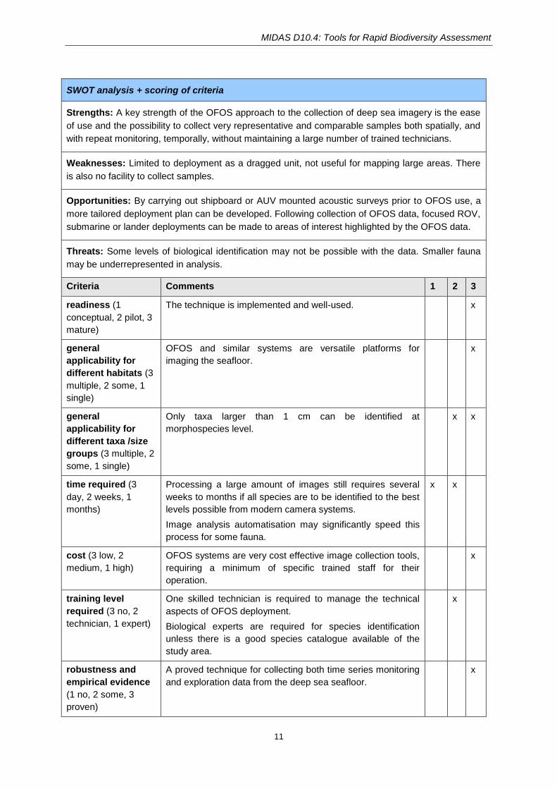
SWOT analysis + scoring of criteria
Strengths: A key strength of the OFOS approach to the collection of deep sea imagery is the ease
of use and the possibility to collect very representative and comparable samples both spatially, and
with repeat monitoring, temporally, without maintaining a large number of trained technicians.
Weaknesses: Limited to deployment as a dragged unit, not useful for mapping large areas. There
is also no facility to collect samples.
Opportunities: By carrying out shipboard or AUV mounted acoustic surveys prior to OFOS use, a
more tailored deployment plan can be developed. Following collection of OFOS data, focused ROV,
submarine or lander deployments can be made to areas of interest highlighted by the OFOS data.
Threats: Some levels of biological identification may not be possible with the data. Smaller fauna
may be underrepresented in analysis.
Criteria Comments 1 2 3
readiness (1
conceptual, 2 pilot, 3
mature)
The technique is implemented and well-used. x
general
applicability for
different habitats (3
multiple, 2 some, 1
single)
OFOS and similar systems are versatile platforms for
imaging the seafloor.
x
general
applicability for
different taxa /size
groups (3 multiple, 2
some, 1 single)
Only taxa larger than 1 cm can be identified at
morphospecies level.
x x
time required (3
day, 2 weeks, 1
months)
Processing a large amount of images still requires several
weeks to months if all species are to be identified to the best
levels possible from modern camera systems.
Image analysis automatisation may significantly speed this
process for some fauna.
x x
cost (3 low, 2
medium, 1 high)
OFOS systems are very cost effective image collection tools,
requiring a minimum of specific trained staff for their
operation.
x
training level
required (3 no, 2
technician, 1 expert)
One skilled technician is required to manage the technical
aspects of OFOS deployment.
Biological experts are required for species identification
unless there is a good species catalogue available of the
study area.
x
robustness and
empirical evidence
(1 no, 2 some, 3
proven)
A proved technique for collecting both time series monitoring
and exploration data from the deep sea seafloor.
x

MIDAS D10.4: Tools for Rapid Biodiversity Assessment
12
representativeness
of different
taxonomical and
functional groups
(1 single, 2 multiple,
3 all)
Particularly useful for identifying even small individuals to
functional group; taxonomical identification is largely
dependent on understanding of the deployed location
ecosystems and the availability of experts.
x
taxonomic
resolution (1
highest: phyla to
order;2 medium:
family to genus;
lowest: 3 species or
OTU)
Difficult to go above family or genus level identification from
even high resolution images alone. This is possible with
sample groundtruthing.
x
spatial coverage (1
cm², 2 m², 3 km²)
Six or seven kilometer surveys can be conducted at optimal
resolution in a 12 hr seafloor deployment. Though the survey
will consist of a transect several meters wide and kilometers
in length rather than a 2D image map.
x
Temporal coverage
(1 snapshot, 2 weeks
to months, 3 year)
Though OFOS surveys are conducted over hours / days, the
ease of deployment of the system and the relative ease of
mounting on research vessels makes the system appealing
for use in monitoring studies with repeat visits to a location
planned.
x
Illustration from a MIDAS case study
During 2015 the JPI Oceans project investigated the manganese nodule fields of the DISCOL
experimental area in the South Pacific with two research cruises. The initial cruise carried out an in-
depth multibeam, backscatter and visual AUV inspection of an area of seafloor from which 90 ~ 6 km
ploughmarks had removed manganese nodules from the seafloor surface. From this survey, a tailored
OFOS campaign allowed 20 deployments to image comparable areas of ploughed, unploughed and
reference areas of the seafloor. By analyzing this collected data, the impact of nodule removal on
fauna larger than 1 cm was evident, and the results are currently being written up in the framework of
MIDAS.
The OFOS deployments at DISCOL also allowed locations for ROV and Lander deployments to be
determined, to collect environmental data and to investigate geochemical processes at the seafloor
with the aim of scaling up the findings spatially.
By conducting the surveys following the protocols outlined above, it is hoped further visits to the region
will allow data on timescales of recolonization to be better determined for fauna.

MIDAS D10.4: Tools for Rapid Biodiversity Assessment
13
2.2. Remotely Operated Vehicles (ROV)
Authors: Ann Vanreusel, Lenaick Menot
Target taxa :
Mobile and sessile
taxa.
Size groups
Megafauna
Spatial resolution
1 cm / Pix
10-100 m2 / Image
Topography
All except when to steep and
heterogeneous
Lowest taxonomic
level resolved
Species (cryptic
species only when
combined with
sampling)
Surface/subsurface
Surface
Sampling
equipment
Some ROV allow
sampling
Substrates
All
Functional group
identification
Based on
morphology
Temporal record
No unless repeated
Image equipment
Video camera
Ecosystems/target deposits
All
Introduction
A Remotely Operated Vehicle (ROV) is an unmanned underwater robot, controlled by a pilot aboard a
vessel. They are connected to the ship by a cable that provides electrical power to the ROV, but also
exchanges in real time video and data signals between the ship and the ROV. Different types and
sizes of ROVs are being used in deep-sea research, with different facilities and capacities for
manoeuvring, imaging and sampling. Also the operational bathymetric range varies between different
ROVs. Many commercial ROVs as operated in the offshore industry can dive to 3000 m, whereas
science ROVs can operate up to abyssal depths (6000 m). Instrumentation can include sonars, video
and still cameras, manipulators, water and sediment samplers, and various sensors.
The advantage of ROVs compared to towed cameras and AUVs is that they can fly above and land
on the seafloor at exact locations. By using cameras and manipulators small and delicate specimens
can be collected more precisely than by any other sampling gear. In this respect it is the only tool that
allows the combination of video imaging with specimen collection.
Protocols including sampling, data collection and data processing
The ROV should be flown at a constant speed of approximately 0.2 m s-1
with a high-definition color
video camera (resolution of minimum 2 mega pixels) approximately 1 m above the seafloor. The
camera ideally needs to be positioned perpendicular to the scene to allow for quantitative estimates
of the area on the video. Transect width can be monitored by using two laser pointers directed at
fixed positions on the seabed. The optical resolution of the camera should enable the reliable
identification of all organisms larger than 3 cm. Smaller organisms are possibly underestimated.
Data processing is similar as for the OFOS system except that annotation can take place real time. A
number of commercial and open-source software can help the annotation process. In general all
megabenthic epifauna can be counted or specific key taxa can be targeted and identified to the
lowest taxonomic level possible; colonial organisms should be counted as single individuals. Uniform
transects lengths (preferably larger than 300 m) and directions should be aimed for but can depend
on local conditions.
The density of each taxonomic group should be standardized to area (e.g., individuals per 100 m2) for
further analysis.
MIDAS D10.4: Tools for Rapid Biodiversity Assessment
14
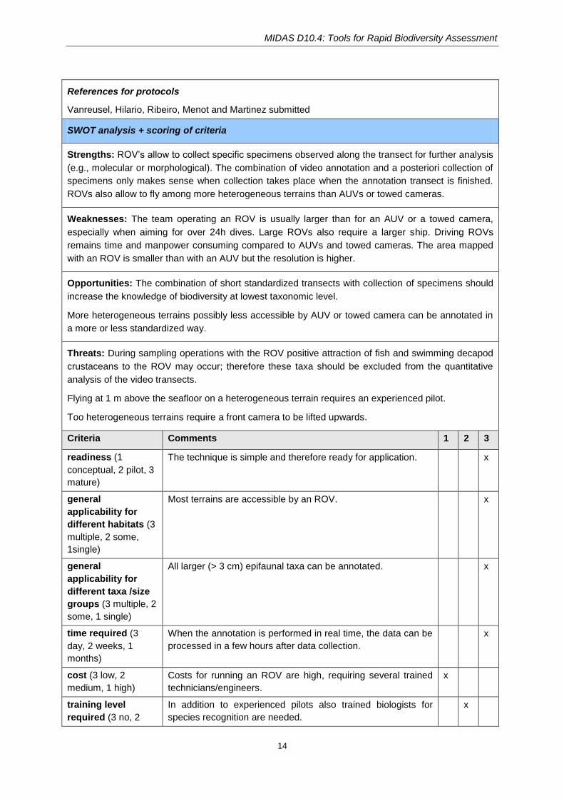
References for protocols
Vanreusel, Hilario, Ribeiro, Menot and Martinez submitted
SWOT analysis + scoring of criteria
Strengths: ROV’s allow to collect specific specimens observed along the transect for further analysis
(e.g., molecular or morphological). The combination of video annotation and a posteriori collection of
specimens only makes sense when collection takes place when the annotation transect is finished.
ROVs also allow to fly among more heterogeneous terrains than AUVs or towed cameras.
Weaknesses: The team operating an ROV is usually larger than for an AUV or a towed camera,
especially when aiming for over 24h dives. Large ROVs also require a larger ship. Driving ROVs
remains time and manpower consuming compared to AUVs and towed cameras. The area mapped
with an ROV is smaller than with an AUV but the resolution is higher.
Opportunities: The combination of short standardized transects with collection of specimens should
increase the knowledge of biodiversity at lowest taxonomic level.
More heterogeneous terrains possibly less accessible by AUV or towed camera can be annotated in
a more or less standardized way.
Threats: During sampling operations with the ROV positive attraction of fish and swimming decapod
crustaceans to the ROV may occur; therefore these taxa should be excluded from the quantitative
analysis of the video transects.
Flying at 1 m above the seafloor on a heterogeneous terrain requires an experienced pilot.
Too heterogeneous terrains require a front camera to be lifted upwards.
Criteria Comments 1 2 3
readiness (1
conceptual, 2 pilot, 3
mature)
The technique is simple and therefore ready for application. x
general
applicability for
different habitats (3
multiple, 2 some,
1single)
Most terrains are accessible by an ROV. x
general
applicability for
different taxa /size
groups (3 multiple, 2
some, 1 single)
All larger (> 3 cm) epifaunal taxa can be annotated. x
time required (3
day, 2 weeks, 1
months)
When the annotation is performed in real time, the data can be
processed in a few hours after data collection.
x
cost (3 low, 2
medium, 1 high)
Costs for running an ROV are high, requiring several trained
technicians/engineers.
x
training level
required (3 no, 2
In addition to experienced pilots also trained biologists for
species recognition are needed.
x
MIDAS D10.4: Tools for Rapid Biodiversity Assessment
15
technician, 1 expert)
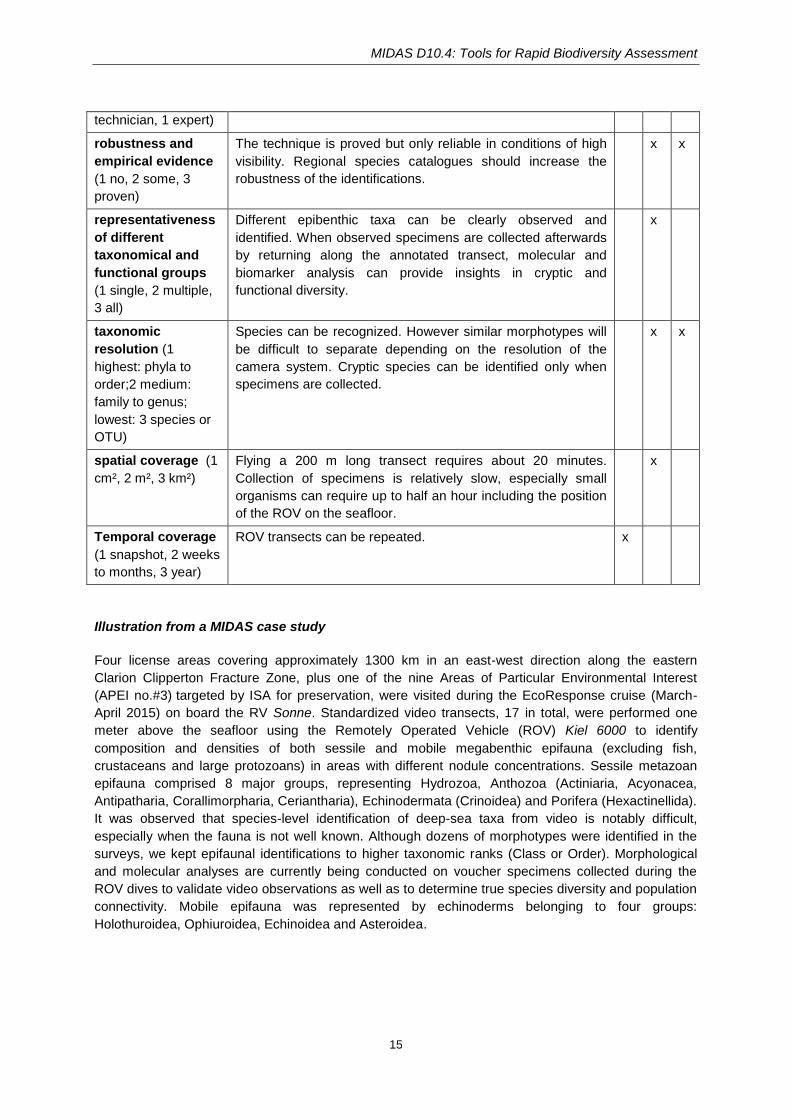
robustness and
empirical evidence
(1 no, 2 some, 3
proven)
The technique is proved but only reliable in conditions of high
visibility. Regional species catalogues should increase the
robustness of the identifications.
x x
representativeness
of different
taxonomical and
functional groups
(1 single, 2 multiple,
3 all)
Different epibenthic taxa can be clearly observed and
identified. When observed specimens are collected afterwards
by returning along the annotated transect, molecular and
biomarker analysis can provide insights in cryptic and
functional diversity.
x
taxonomic
resolution (1
highest: phyla to
order;2 medium:
family to genus;
lowest: 3 species or
OTU)
Species can be recognized. However similar morphotypes will
be difficult to separate depending on the resolution of the
camera system. Cryptic species can be identified only when
specimens are collected.
x x
spatial coverage (1
cm², 2 m², 3 km²)
Flying a 200 m long transect requires about 20 minutes.
Collection of specimens is relatively slow, especially small
organisms can require up to half an hour including the position
of the ROV on the seafloor.
x
Temporal coverage
(1 snapshot, 2 weeks
to months, 3 year)
ROV transects can be repeated. x
Illustration from a MIDAS case study
Four license areas covering approximately 1300 km in an east-west direction along the eastern
Clarion Clipperton Fracture Zone, plus one of the nine Areas of Particular Environmental Interest
(APEI no.#3) targeted by ISA for preservation, were visited during the EcoResponse cruise (March-
April 2015) on board the RV Sonne. Standardized video transects, 17 in total, were performed one
meter above the seafloor using the Remotely Operated Vehicle (ROV) Kiel 6000 to identify
composition and densities of both sessile and mobile megabenthic epifauna (excluding fish,
crustaceans and large protozoans) in areas with different nodule concentrations. Sessile metazoan
epifauna comprised 8 major groups, representing Hydrozoa, Anthozoa (Actiniaria, Acyonacea,
Antipatharia, Corallimorpharia, Ceriantharia), Echinodermata (Crinoidea) and Porifera (Hexactinellida).
It was observed that species-level identification of deep-sea taxa from video is notably difficult,
especially when the fauna is not well known. Although dozens of morphotypes were identified in the
surveys, we kept epifaunal identifications to higher taxonomic ranks (Class or Order). Morphological
and molecular analyses are currently being conducted on voucher specimens collected during the
ROV dives to validate video observations as well as to determine true species diversity and population
connectivity. Mobile epifauna was represented by echinoderms belonging to four groups:
Holothuroidea, Ophiuroidea, Echinoidea and Asteroidea.

MIDAS D10.4: Tools for Rapid Biodiversity Assessment
16
2.3. Autonomous Underwater Vehicles
Authors: Daniel Jones, Timm Schoening
Target taxa :
All mobile and
sessile taxa.
Size groups
Megafauna
Spatial resolution
1 cm / Pix
Abyss: 100 m2 /
Image
Topography
Generally flat (Slope < 10%)
Lowest taxonomic
level resolved
Species (excl cryptic
species)
Surface and
subsurface
Surface
Sampling
equipment
No physical
samples. Sensor-
based assessments
only
Substrates
All
Functional group
identification
Based on
morphology
Temporal record
Only with repeated
surveys
Image equipment
Still camera x2.
Acoustic imaging
(side-scan and
multibeam).
Ecosystems/target deposits
Used in many ecosystems,
including coral reefs, canyons,
abyssal plains.
Introduction
There has been an increased use of image data for marine ecological surveys, both for faunal
surveys, measurements of animal activity, and the study of particulate organic matter supply to the
seafloor (Bett et al., 2001; Smith et al., 2013). Non-bottom contact photographic methods have the
ability to cover a large seafloor area with little environmental impact. They allow fauna that are often
poorly represented by other sampling methods to be observed and identified (Rice et al., 1982), and
can allow local environmental data to be recorded such as habitat and resource availability
(Svoboda, 1985; Bett et al., 1995). Quantitative and spatially explicit data can be collected over
moderate to very large areas at a definable resolution.
Off-bottom towed cameras, such as the NOC Wide Angle Seabed Photography (WASP; Jones et
al., 2009) system, provide within-transect spatial data. However, there are difficulties with controlling
the position, altitude and speed of the camera as it is tethered to the surface vessel and so is
influenced by swell. This can lead to a large proportion of photographs being unsuitable for
quantitative analysis (Jones et al., 2007). On-bottom towed camera sleds do have better stability,
but may be more destructive of the seabed habitat and can have image quality issues from induced
turbidity (Wakefield and Genin, 1987).
Remotely operated vehicles (ROVs) and human occupied vehicles (HOVs) have also been used to
collect photographic and video data, allowing topographically complex habitats to be studied,
including deep-sea vent and cold-water coral sites (Morris et al., 2012; 2013; Wheeler et al., 2013).
These vehicles may also permit the collection of voucher specimens for identification. However,
they have drawbacks for large-scale surveying such as slow transect speeds and large amounts of
ship time being required for their operation, as well as the influence of swell, and difficulty holding a
constant depth due to the tether connection to the tender vessel and limited thruster power. Both
can also induce major fish disturbance from hydraulic noise and continuous flood lighting, leading to
systematic error in density estimates (e.g., Stoner et al., 2008).
In contrast, AUVs provide stable imaging platforms that can be operated close to the seafloor in
suitable areas, produce less noise than ROVs or HOVs, and do not require continuous lighting.
They are capable of sustained operations while the surface vessel is engaged in other work,
reducing the ship time dedicated to their operation. It has been long expected that use of AUVs

MIDAS D10.4: Tools for Rapid Biodiversity Assessment
17
would rapidly increase our knowledge of the distribution of visible megafauna at landscape scales
(Forman and Godron, 1986).
Equipment description
Autosub6000 is an autonomous underwater vehicle measuring 5.5 m in length and 0.9 m in
diameter, having a weight in air of 1800 kg. Fitted with lithium polymer rechargeable batteries, it can
operate for ~48 hours at a speed of 1.7 m s-1
. It has an IXSEA Photonic Inertial Navigation System
(PHINS) and an RDI Teledyne Workhorse Navigator Acoustic Doppler Current Profiler (ADCP) to
enable underwater navigation. A Tritech SeaKing scanning sonar is employed for obstacle
avoidance. Two-way communications with the vehicle are achieved via a LinkQuest Tracklink
10000 ultra-short baseline (USBL) system. At the surface communication is possible via a WiFi
radio link (Morris et al., 2014).
As deployed for MIDAS (JC120), the vehicle carried a sensor suite including: dual conductivity,
temperature and depth (CTD) system; optical backscatter-based turbidity sensor; tri-axial
magnetometer; 300 kHz ADCP; sidescan sonar; sub-bottom profiler; and multibeam echosounder.
In addition to these standard sensors, two cameras (one downward-facing and one oblique forward-
facing) were also fitted. Point Grey Research Inc. Grasshopper 2 cameras were employed, with a
2/3” sensor (2,448 x 2,048 pixels, i.e. 5 Mega-pixel). A 12 mm focal length lens with horizontal and
vertical acceptance angles of the cameras were 26.71° and 22.65°, respectively, was used (Morris
et al., 2014). The downward camera was mounted at 90° to the long-axis of the vehicle in its
forward section. The oblique camera was mounted in the nose of the vehicle, and aimed 35° below
the long-axis. Distance between cameras is 686 mm. A NOC designed xenon strobe unit was used
with each camera (11 J, with 2 Hz potential repetition rate) mounted along a parallel direction to the
camera angle. The frontal facing camera is separated 180 mm from its corresponding flash,
whereas the vertical camera is 430 mm separated from its flash.
The Autonomous Underwater Vehicle (AUV) Abyss (built by HYDROID Inc.) from GEOMAR can be
operated in water depths up to 6000 m. The system comprises the AUV itself, a control and
workshop container, and a mobile Launch and Recovery System (LARS) with a deployment frame.
The AUV Abyss can be launched and recovered at weather conditions with a swell up to 2.5 m and
wind speeds of up to 6 Beaufort. Primary sensors are the RESON Seabat 7125 (multibeam; 200
kHz), the Deep Survey camera and the Edgetech sidescan sonar.
Protocols including sampling, data collection and data processing
i) AutoSub
Sampling / data collection
AUV mission planning used all available data on the vehicle endurance and seabed terrain to plan
data acquisition appropriate for the investigation of the scientific hypotheses being tested. For
imagery missions multiple survey strategies are possible, including replicated transects and
complete or partial coverage ‘moving the lawn’ surveys. Bespoke mission planning software
automated the creation of waypoints for regular survey strategies (e.g., grids). AUV missions were
planned in geographic information system software. The operational constraints of the vehicle were
assessed throughout to reduce the mission risk. This was principally achieved using ship-board
multibeam bathymetry data and ideally higher resolution AUV-obtained multibeam (100 m altitude)
to ensure that the terrain was relatively flat (slope < 10%). Once a survey was designed and
checked, waypoints were exported and converted with vehicle directions (e.g., altitude, time cut-
offs, etc.) into mission code for the AUV. Mission codes were loaded onto vehicle systems via WiFi.
The vehicle was launched using a bespoke launch and recovery system. Once in the water, the
MIDAS D10.4: Tools for Rapid Biodiversity Assessment
18
vehicle acquired a GPS location fix at the surface and a command to initiate the mission was sent to
the vehicle via WiFi. The vehicle then dived and began a helical descent to the target altitude. The
acoustic modem was used to transfer engineering data to allow monitoring of the operation. When
within c. 100 m of the seafloor the Doppler Velocity Log (DVL) became effective in tracking the AUV
relative to the seafloor. Both the DVL and the inertial navigation data were combined to give the
location of the vehicle. To adjust for any navigational offset accrued during the descent phase, the
vehicle started the survey with a navigation box with 1 km sides. The position of the vehicle was
monitored from the surface vessel via the USBL system, and any offset from the intended location
of the navigation box was calculated and transmitted to the AUV (McPhail and Pebody, 2009). The
vehicle then updated its absolute geo-location before commencing the science mission (Morris et
al., 2014).
Autosub6000 was operated at a target altitude of 3.2 m for photographic missions. At a target
altitude of 3.2 m the downward camera captures an image of 2.4 m2 of seabed, with the oblique
camera imaging an area of approx 16.5 m2
(Morris et al., 2014). The submersible speed was 1.2 m
s-1
, and the interval between pictures was set at 850 milliseconds. Over a typical ~ 100 km
photographic mission (~30 hours) around 100,000 images were obtained from each camera, with
vertical images covering a seabed area of 250,000 m2.
A PC104-based data logger on the AUV stored engineering data (navigation processor, control
sensors, actuation systems) and lower-rate science data (CTD), which was downloaded post-
mission via WiFi. High-rate sensors (multibeam, sidescan sonar, sub-bottom profiler, cameras) had
their own integral hard drives, accessible over Ethernet (and WiFi). Transfer of large numbers of
photographs was most effectively achieved via cabled transfer from the hard drive at the end of
each mission. Engineering, navigation and science data (e.g., CTD) were recorded at 2 second
intervals. These data were then interpolated to provide water depth, altitude, heading, pitch, roll and
geo-location for each seafloor image (0.87 second camera repetition rate). The time period for
which the camera took images was determined by considering the nominal velocity of the AUV over
the seafloor, the degree of overlap required for tiling, the angular view and camera resolution as
well as the target altitude for the camera (which was set at 3.2 m) for optimal visibility of the seafloor
as well as possible identification of smaller animals. The image interval and altitude can be changed
dependent on the required outcomes of the missions (Morris et al., 2014).
Data processing
The AUV image data is suitable for many purposes, such as gauging seafloor coverage by
pollutants, seafloor coverage by habitat types, fauna seafloor coverage by area and / or
abundances, etc. How these images are processed depends to a large extent on the aim of the
study and the required level of detail. In areas where particular fauna or seafloor features are
abundant or distinctive in appearance, it may be possible to use learning algorithms to automatically
assess abundances or coverage across the collected image data set, via systems such as BIIGLE
(Purser et al., 2009; Schoening et al., 2012).
The most commonly used data processing protocol used with Autosub6000 images is as follows:
Image processing:
Following initial inspection, only images from linear track segments (e.g. vehicle turns excluded)
where the vehicle altitude was between 1.9 and 4.1 m were processed further. These images were
subject to manipulation implemented via a MatlabV2013a (Mathworks) script as below (further detail
in Morris et al., 2014).
Dark frame removal: Fifty images from an altitude of 15-30 m were selected, representing control
MIDAS D10.4: Tools for Rapid Biodiversity Assessment
19
images without seafloor image data. The mean pixel value was calculated to derive an average
‘black frame’ image and thus the mean level of ‘noise’, observed within the images. This black
frame image was subtracted from each seafloor image before further processing. This was
repeated for each individual mission.
Non-uniform illumination correction: Fifty seafloor images (1.9-4.1 m altitude) were selected at
random within a given mission. For each pixel position in the image the mean intensity was
calculated. The mean intensity value was then used to equalise each image in an attempt to
minimise illumination vignetting (a reduction in image brightness or saturation at the periphery)
before analysis.
Colour correction: The light path (from flash to seafloor to image sensor) for each image pixel was
calculated from the vehicle altitude, assuming the sensor plane was parallel to the seafloor.
Individual pixels in the red, green, and blue channels were corrected for percentage light loss
assuming the clear type I (oceanic) light attenuation values given by Chiang and Chen (2012).
Geo-referencing: Interpolated latitude and longitude (WGS84) values from the vehicle’s navigation
record were assigned to the center of each image. To allow the area of the images to be calculated
a conversion to the Universal Transverse Mercator (UTM) projected coordinate system was
undertaken. A three dimensional rotation was then applied to correct for vehicle heading, pitch, and
roll. The image was the re-projected to seabed level, and corresponding seafloor dimensions and
geographic position to be obtained. The re-sampled images were output in GeoTIFF format
(http://trac.osgeo.org/geotiff/), with geo-location data in UTM coordinates.
Removing overlap: Overlap between adjacent pairs of vertical images was determined by geo-
location, and removed by cropping half of the overlap from each. Given the vehicle’s speed, altitude
and camera acceptance angles, adjacent images were c. 15% overlapped.
Image annotation and data generation
Each image was opened in Image Pro Plus V7 (Media Cybernetics) and a further brightness
histogram correction was applied before annotation to brighten the image, allowing organisms to be
more visible. Annotation was completed using a custom macro that allowed individual organisms
within the tiles to be indicated, categorised according to morphotype and measured. The software
produced an output database containing the morphotype identification, a nominal label, length in
pixels and location coordinates of the organism’s central point. This pixel-based data was then
combined with the embedded geo-location data (GeoTIFF) to convert to ‘real-world’ units. The
seafloor area covered by each tile was calculated, and faunal count data were converted to spatial
density units.
ii) Abyss
Imaging missions are planned either in an “exploratory” or “mosaicking” mode. Exploratory missions
are conducted in unknown areas to cover as much seafloor as possible but with limited overlap
between images. High overlap is targeted in the mosaicking mode to be able to find
correspondences in individual images that allow the creation of large areal overviews of habitats.
AUV Abyss can be deployed around the clock and is intermittently monitored from the surface
vessel if traveling in close vicinity. Abyss records environmental parameters (CTD, Turbidity,
Chlorophyll) as well as navigation data (yaw, pitch, roll, lat, lon, etc.) during each mission.
Images obtained by the Deep Survey Camera are corrected for FishEye distortion and colour
attenuation. Fusion of environmental, navigation and image data is conducted and long term
archival in the GEOMAR media database is implemented.
MIDAS D10.4: Tools for Rapid Biodiversity Assessment
20
References for protocols
Bett BJ, Rice AL. Thurston MH (1995) A quantitative photographic survey of "spoke-burrow" type
lebensspuren on the Cape Verde Abyssal Plain. Int. Rev ges Hydrobio, Berlin 80:153-170.
Bett BJ, Malzone MG, Narayanaswamy BE, Wigham BD (2001) Temporal variability in phytodetritus
and megabenthic activity at the seabed in the deep northeast Atlantic. Progress in Oceanography
50: 349-368.
Chiang JY, Chen YC (2012) Underwater image enhancement by wavelength compensation and
dehazing. IEEE Trans Image Process. 21: 1755-1769. doi:10.1109/TIP.2011.2179666.
Forman RTT, Godron M (1986) Landscape ecology. Wiley, New York.
Jones DOB, Bett BJ, Tyler PA (2007) Megabenthic ecology of the deep Faroe-Shetland Channel: a
photographic study. Deep-Sea Research I 54: 1111-1128.
Jones DOB, Bett BJ, Wynn RB, Masson DG (2009) The use of towed camera platforms in deep-
water science. Int J. Soc. Underw. Technol. 28: 41-50.
Kwasnitschka T, et al. (2016) "DeepSurveyCam—A Deep Ocean Optical Mapping System."
Sensors 16.2: 164.
McPhail SD, Pebody M (2009) Range-only positioning of a deep-diving Autonomous Underwater
Vehicle from a surface ship. IEEE Journal of Oceanic Engineering 34(4): 669-677.
doi:10.1109/JOE.2009.2030223.
Morris KJ, Tyler PA, Murton B, Rogers AD (2012) Lower bathyal and abyssal distribution of coral in
the axial volcanic ridge of the Mid-Atlantic Ridge at 45° N. Deep-Sea Research I 62: 32-39.
Morris KJ, Tyler PA, Masson DG, Huvenne VAI, Rogers AD (2013) Distribution of cold-water corals
in the Whittard Canyon, NE Atlantic Ocean. Deep-Sea Research II 92: 136–144.
Morris KJ, Bett BJ, Durden JM, Huvenne VAI, Milligan R, Jones DOB, McPhail S, Robert K, Bailey
DM, Ruhl HA (2014) A new method for ecological surveying of the abyss using autonomous
underwater vehicle photography. Limnology and Oceanography Methods 12: 795-809.
Purser A, Bergmann M, Lundalv T, Ontrup J, Nattkemper TW (2009) Use of machine-learning
algorithms for the automated detection of cold-water coral habitats: a pilot study. Marine Ecology
Progress Series 397: 241-251.
Rice AL, Aldred RG, Darlington E, Wild RA (1982) The quantitative estimation of the deep-sea
megabenthos: a new approach to an old problem. Oceanol. Acta 5:63-72.
Schoening T, Bergmann M, Ontrup J, Taylor J, Dannheim J, Gutt J, Purser A, Nattkemper TW
(2012) Semi-Automated Image Analysis for the Assessment of Megafaunal Densities at the Arctic
Deep-Sea Observatory HAUSGARTEN. PLoS ONE 7(6): e38179.
Smith KL, Ruhl HA, Kahru M, Huffard CL, Sherman AD (2013) Deep ocean communities impacted
by changing climate over 24 y in the abyssal northeast Pacific Ocean. Proc. Nat. Acad. Sci. 110:
19838-19841.
Stoner AW, Ryer CH, Parker SJ, Auster PJ, Wakefield WW (2008) Evaluating the role of fish
behavior in surveys conducted with underwater vehicles. Can. J. Fish. Aquat. Sci. 65:1230–1243.
Svoboda A (1985) Diver-operated cameras and their marine-biological uses. In JD George, Lythgoe
GI, Lythgoe JN (eds.) Underwater photography and television for scientists. Clarendon Press,
Oxford.
MIDAS D10.4: Tools for Rapid Biodiversity Assessment
21
Wakefield WW, Genin A (1987) The use of a Canadian (perspective) grid in deep sea photography.
Deep Sea Res. 34: 469-478.
Wheeler AJ, Murton B, Copley J, Lim A, Carlsson J, Collins P, Dorschel B, Green D, Judge M, Nye
V, Benzie J, Antoniacomi A, Coughlan M, Morris K (2013) Moytirra: Discovery of the first known
deep‐sea hydrothermal vent field on the slow-spreading Mid-Atlantic Ridge north of the Azores.
Geochem., Geophys., Geosyst. 14: 4170–4184.
SWOT analysis + scoring of criteria
Strengths: AUV imagery allows the collection of large amounts of deep-sea imagery in a short time
frame. The AUV is also a very stable platform, which collects positional and altitude data alongside
each image – greatly facilitating automated image processing and analysis. It can be used for
mapping large areas in high detail. The AUV also allows other work to be carried out concurrently
with data collection.
Weaknesses: The AUV is complex and requires a team of highly-trained technicians to operate. It
can only be deployed from large research vessels. This type of AUV cannot be used in areas of
high topographic variability.
As with all imaging methods, the taxonomic resolution of data may be relatively low. Identification to
species level is likely not possible for many groups, particularly in poorly studied regions. Smaller
fauna, infauna and cryptic species (both hiding/camouflaged and morphologically similar species)
are difficult or impossible to detect.
Opportunities: Multiple other types of AUV platform exist, which could augment data collected with
an AUV such as Autosub6000. Hover-capable vehicles and crawlers could both be used in a similar
way. Used in conjunction with ROV, precision samples to improve taxonomic resolution can be
obtained.
Threats: Smaller, less complex and cheaper imaging platforms may be used in some studies.
Image analysis is usually manual and is a major bottleneck. Platform loss is expensive (> 1Mio €).
No live streaming of data possible so changes in research plans can only be done after AUV
recovery and data analysis.
Criteria Comments 1 2 3
readiness (1
conceptual, 2 pilot, 3
mature)
This technique is implemented and used on multiple
occasions. The vehicle is still somewhat developmental.
x x
general
applicability for
different habitats (3
multiple, 2 some, 1
single)
This platform may be used on multiple, but not all habitats.
High relief (topography) habitats cannot be investigated.
x
general
applicability for
different taxa /size
groups (3 multiple, 2
some, 1 single)
Only taxa larger than 1 cm can be identified at
morphospecies level.
x x
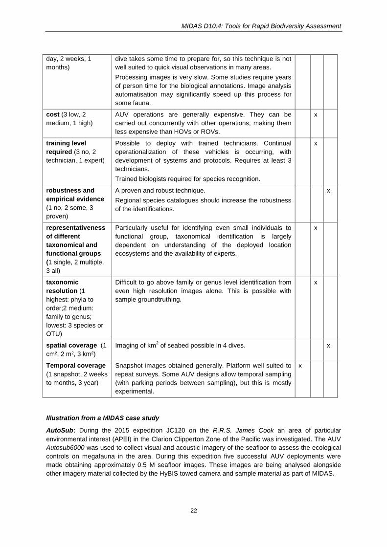
time required (3 Image acquisition is very quick within a study area. Each x x
MIDAS D10.4: Tools for Rapid Biodiversity Assessment
22
day, 2 weeks, 1
months)
dive takes some time to prepare for, so this technique is not
well suited to quick visual observations in many areas.
Processing images is very slow. Some studies require years
of person time for the biological annotations. Image analysis
automatisation may significantly speed up this process for
some fauna.
cost (3 low, 2
medium, 1 high)
AUV operations are generally expensive. They can be
carried out concurrently with other operations, making them
less expensive than HOVs or ROVs.
x
training level
required (3 no, 2
technician, 1 expert)
Possible to deploy with trained technicians. Continual
operationalization of these vehicles is occurring, with
development of systems and protocols. Requires at least 3
technicians.
Trained biologists required for species recognition.
x
robustness and
empirical evidence
(1 no, 2 some, 3
proven)
A proven and robust technique.
Regional species catalogues should increase the robustness
of the identifications.
x
representativeness
of different
taxonomical and
functional groups
(1 single, 2 multiple,
3 all)
Particularly useful for identifying even small individuals to
functional group, taxonomical identification is largely
dependent on understanding of the deployed location
ecosystems and the availability of experts.
x
taxonomic
resolution (1
highest: phyla to
order;2 medium:
family to genus;
lowest: 3 species or
OTU)
Difficult to go above family or genus level identification from
even high resolution images alone. This is possible with
sample groundtruthing.
x
spatial coverage (1
cm², 2 m², 3 km²)
Imaging of km2 of seabed possible in 4 dives. x
Temporal coverage
(1 snapshot, 2 weeks
to months, 3 year)
Snapshot images obtained generally. Platform well suited to
repeat surveys. Some AUV designs allow temporal sampling
(with parking periods between sampling), but this is mostly
experimental.
x
Illustration from a MIDAS case study
AutoSub: During the 2015 expedition JC120 on the R.R.S. James Cook an area of particular
environmental interest (APEI) in the Clarion Clipperton Zone of the Pacific was investigated. The AUV
Autosub6000 was used to collect visual and acoustic imagery of the seafloor to assess the ecological
controls on megafauna in the area. During this expedition five successful AUV deployments were
made obtaining approximately 0.5 M seafloor images. These images are being analysed alongside
other imagery material collected by the HyBIS towed camera and sample material as part of MIDAS.

MIDAS D10.4: Tools for Rapid Biodiversity Assessment
23
Abyss: During the 2015 expeditions SO239 (“Ecomining Impact”) and SO242-1 (“DISCOL revisited”),
Abyss was deployed with the DeepSurvey Camera for the first time. In total, 12 (9) dives were
conducted during SO239 (SO242-1). Several manganese nodule claims were imaged as well as an
Area of Particular Environmental interest and the DISCOL Experimental Area. More than 500,000
images were recorded representing 8.3 km2 of abyssal seafloor.

MIDAS D10.4: Tools for Rapid Biodiversity Assessment
24
3. Sample-based techniques
MIDAS D10.4: Tools for Rapid Biodiversity Assessment
25
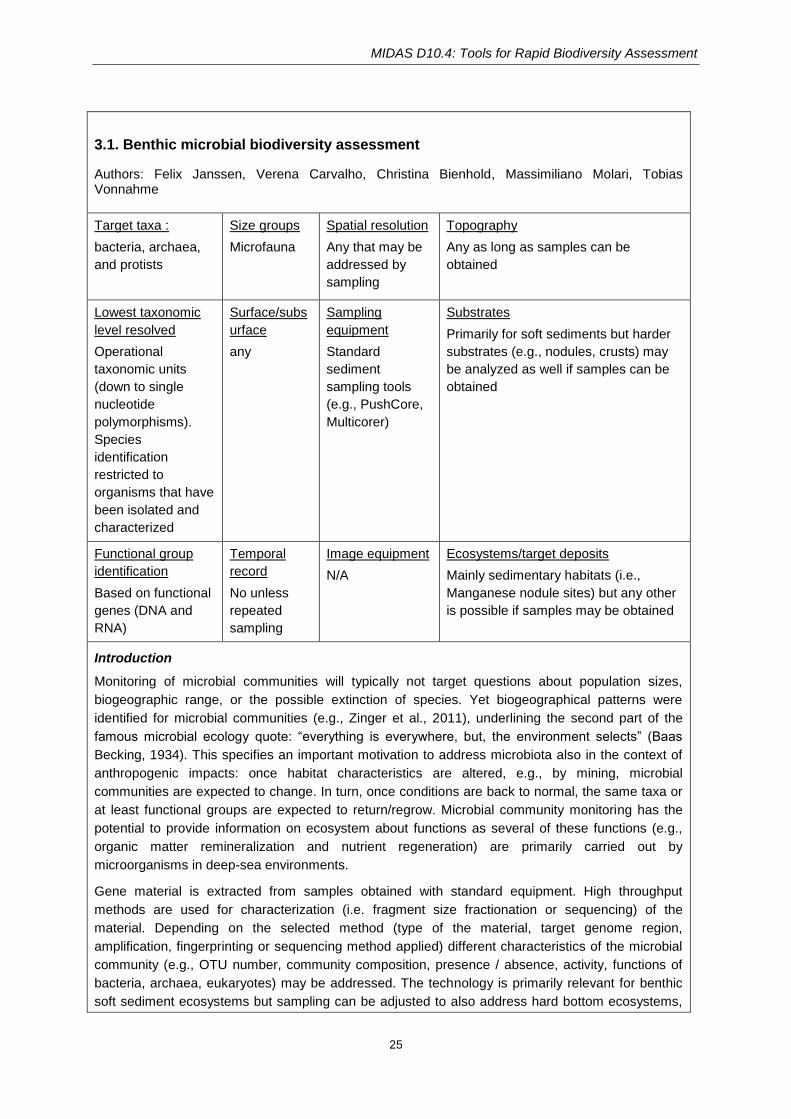
3.1. Benthic microbial biodiversity assessment
Authors: Felix Janssen, Verena Carvalho, Christina Bienhold, Massimiliano Molari, Tobias Vonnahme
Target taxa :
bacteria, archaea,
and protists
Size groups
Microfauna
Spatial resolution
Any that may be
addressed by
sampling
Topography
Any as long as samples can be
obtained
Lowest taxonomic
level resolved
Operational
taxonomic units
(down to single
nucleotide
polymorphisms).
Species
identification
restricted to
organisms that have
been isolated and
characterized
Surface/subs
urface
any
Sampling
equipment
Standard
sediment
sampling tools
(e.g., PushCore,
Multicorer)
Substrates
Primarily for soft sediments but harder
substrates (e.g., nodules, crusts) may
be analyzed as well if samples can be
obtained
Functional group
identification
Based on functional
genes (DNA and
RNA)
Temporal
record
No unless
repeated
sampling
Image equipment
N/A
Ecosystems/target deposits
Mainly sedimentary habitats (i.e.,
Manganese nodule sites) but any other
is possible if samples may be obtained
Introduction
Monitoring of microbial communities will typically not target questions about population sizes,
biogeographic range, or the possible extinction of species. Yet biogeographical patterns were
identified for microbial communities (e.g., Zinger et al., 2011), underlining the second part of the
famous microbial ecology quote: “everything is everywhere, but, the environment selects” (Baas
Becking, 1934). This specifies an important motivation to address microbiota also in the context of
anthropogenic impacts: once habitat characteristics are altered, e.g., by mining, microbial
communities are expected to change. In turn, once conditions are back to normal, the same taxa or
at least functional groups are expected to return/regrow. Microbial community monitoring has the
potential to provide information on ecosystem about functions as several of these functions (e.g.,
organic matter remineralization and nutrient regeneration) are primarily carried out by
microorganisms in deep-sea environments.
Gene material is extracted from samples obtained with standard equipment. High throughput
methods are used for characterization (i.e. fragment size fractionation or sequencing) of the
material. Depending on the selected method (type of the material, target genome region,
amplification, fingerprinting or sequencing method applied) different characteristics of the microbial
community (e.g., OTU number, community composition, presence / absence, activity, functions of
bacteria, archaea, eukaryotes) may be addressed. The technology is primarily relevant for benthic
soft sediment ecosystems but sampling can be adjusted to also address hard bottom ecosystems,
MIDAS D10.4: Tools for Rapid Biodiversity Assessment
26
and even the water column. Although sequencing workflows are well established and often carried
out by commercial labs, the interest to investigate the biodiversity and function of benthic microbial
communities is so far largely limited to academia. A reason might be standardized procedures are
hard to establish when molecular techniques and data analysis workflows evolve fast. The resulting
need for expert knowledge and the limited operability still confine routine use for monitoring
purposes. Another reason is that the relevance in the context of monitoring anthropogenic impacts
is not yet fully established.
Baas Becking LGM (1934) Geobiologie of inleidung tot de milieukunde. WP van Stockum & Zoon,
Den Haag.
Zinger L, Amaral-Zettler LA, Fuhrman JA, Horner-Devine MC, Huse SM, Welch DBM, Martiny JBH,
Sogin M, Boetius A, Ramette A (2011) Global Patterns of Bacterial Beta-Diversity in Seafloor and
Seawater Ecosystems, PLoS ONE 6(9): e24570. doi:10.1371/journal.pone.0024570.
Protocols including sampling, data collection and data processing
Sampling
Sampling of sediment is carried out with standard gear (e.g., ROV Push Core, Multicorer). Samples
are stored (frozen, best at -80°C) with or without prior treatment with storage reagent (e.g.,
RNAlater). Sampling of hard substrates or bottom waters requires other instruments (e.g., grabs,
CTD/Rosette samplers) and additional sample preparation steps (grinding, filtering). Gene material
is extracted from the samples using a combination of physical and chemical methods and typically
involves commercially available extraction kits.
Sample and data analysis
A suite of analytical methods targeting DNA, rRNA, and mRNA sequences, as well as copy
numbers is currently available which either involve amplification (PCR, qPCR, RT-PCR, MDA) or
not (metagenomics and -transcriptomics). These analyses as well as the subsequent sequencing
step are high throughput methods and are typically performed by dedicated commercial
laboratories.
Depending on (1) the type of the material (DNA, rRNA, mRNA), (2) the specific region of the
genome addressed (e.g., V3 & V4 16S rRNA region, V9 18S rRNA region), (3) preceding
amplification steps (PCR, qPCR) and (4) the fingerprinting (e.g., T-RFLP, ARISA) or sequencing
method used (Next Generation Sequencing (NGS), e.g., 454 pyrosequencing, Ilumina, PacBio) data
analysis may differ and / or address different aspects (i.e. compartments, characteristics) of the
microbial community. Targeted aspects typically include (1) the domain that is addressed (bacteria,
archaea, eukaryotes), (2) number of operational taxonomic units (OTUs) present, (3) presence /
absence, and (4) activity of specific taxa/OTUs. If appropriate knowledge (e.g., on functions of
specific genes and typical copy numbers) is available, analyses may additionally target (1)
abundance / dominance of specific groups as well as (2) potential metabolic functions and (3) their
expression.
Community fingerprinting techniques (e.g., Terminal Restriction Fragment Length Polymorphism, T-
RFLP; Denaturing Gradient Gel Electrophoresis, DGGE; Automated Ribosomal Intergenic Spacer
Analysis, ARISA) are used to assess microbial biodiversity by detecting the abundance of target
gene variants present in the sample. Sequencing of rRNA genes is typically used to address
microbial taxonomy, and the diversity of the community. Functional genes are sequenced in order to

MIDAS D10.4: Tools for Rapid Biodiversity Assessment
27
obtain insights into potential functions that are present in the community, while mRNA sequencing
provides information on their expression. In order to analyze the community in even greater depth,
quantitative PCR of rRNA, functional genes, and mRNA/cDNA allows identification of the dominant
taxa, as well as the prevailing (potential or expressed) functions.
Following quality control, comparative and statistical analyses are performed in order to classify
genes and to deduce taxonomy, functional gene repertoire, as well as potential and expressed
metabolic functions.
References for protocols
Methods for nucleic acid preparation and storage
Gorokhova E (2005) Effects of preservation and storage of microcrustraceans in RNAlater on RNA
and DNA degradation. Limnology and Oceanography: Methods 3: 143-148.
Stewart FJ (2013) Preparation of microbial community cDNA for metatranscriptomic analysis in
marine plankton. Methods in Enzymology 531: 187-218.
Fingerprinting methods
Marsh TL (1999) Terminal restriction fragment length polymorphism (T-RFLP): an emerging method
for characterizing diversity among homologous populations of amplification products. Current
Opinion in Microbiology 2: 323-327.
Muyzer G, Smalla K (1998) Application of denaturing gradient gel electrophoresis (DGGE) and
temperature gradient gel electrophoresis (TGGE) in microbial ecology. Antonie van Leeuwenhoek
73: 127-141.
Nocker A, Burr M, Camper AK (2007) Genotypic microbial community profiling: a critical technical
review. Microbial Ecology 54: 276-289.
Next generation sequencing (NGS) methods
Caporaso JG, Lauber CL, Walters WA, Berg-Lyons D, Huntley J, Fierer N, Owens SM, Betley J,
Fraser L, Bauer M, Gormley N, Gilbert JA, Smith G, Knight R (2012) Ultra-high-throughput microbial
community analysis on the Illumina HiSeq and MiSeq platforms. ISME Journal 6: 1621-1624. doi:
10.1038/ismej.2012.8.
Cruaud P, Vigneron A, Lucchetti-Miganeh C, Ciron PE, Godfroy A, Cambon-Bonavita MA (2014)
Influence of DNA extraction method, 16S rRNA targeted hypervariable regions, and sample origin
on microbial diversity detected by 454 pyrosequencing in marine chemosynthetic ecosystems.
Applied and Environmental Microbiology 15: 4626-4639.
Luo C, Tsementzi D, Kyrpides N, Read T, Konstantinidis KT (2012) Direct comparisons of Illumina
vs. Roche 454 sequencing technologies on the same microbial community DNA sample. PloS One
7(2): e30087.
Application of NGS for assessing phylogenetic microbial diversity
Bienhold C, Zinger L, Boetius A, Ramette A (2016) Diversity and Biogeography of Bathyal and
Abyssal Seafloor Bacteria. PloS One 1: e0148016.
Christen R (2008) Global sequencing: a review of current molecular data and new methods

MIDAS D10.4: Tools for Rapid Biodiversity Assessment
28
available to assess microbial diversity. Microbes and Environments 23: 253-268.
Jacob M, Soltwedel T, Boetius A, Ramette A (2013) Biogeography of deep-sea benthic bacteria at
regional scale (LTER HAUSGARTEN, Fram Strait, Arctic). PloS One 9: e72779.
Zinger L, Gobet A, Pommier T (2012) Two decades of describing the unseen majority of aquatic
microbial diversity. Molecular Ecology 8: 1878-1896.
Omics technologies to assess biodiversity by functionality
Gilbert JA, Dupont CL (2011) Microbial Metagenomics: beyond the genome. Annual Review of
Marine Science 3: 347-371.
Moran MA, Satinsky B, Gifford SM, Luo H, Rivers A, Chan L-K, Meng J, Durham BP, Shen C,
Varaljay VA, Smith CB, Yager PL, Hopkins BM (2013) Sizing up metatranscriptomics. The ISME
Journal 7: 237-243.
Nikolaki S, Tsiamis G (2013) Microbial diversity in the era of omic technologies. BioMed Research
International:1-15.
Warnecke F, Hugenholtz P (2007) Building on basic metagenomics with complementary
technologies. Genome Biology 8: 231. doi:10.1186/gb-2007-8-12-231.
Statistical analysis
Buttigieg PL, Ramette A (2014) A guide to statistical analysis in microbial ecology: a community-
focused, living review of multivariate data analyses. FEMS Microbiology: Ecology. doi:
10.1111/1574-6941.12437.
'GUSTA ME' guide to statistical analysis in microbial ecology: http://mb3is.megx.net/gustame
SWOT analysis + scoring of criteria
Strengths: The analysis can be applied to any ecosystem / deposit where samples can be
obtained. Any taxon of the microbial community can be addressed at any possible taxonomic
resolution.
Weaknesses: Standardization of target genome regions and data analysis workflows not yet
achieved. Part of the workflow requires experts. Individual analyses are snapshots in space and
time only. Relevance in the context of (mining) impacts not fully assessed and target taxa and
functions in the context of environmental impact studies not identified yet.
Opportunities: A very dynamic scientific discipline: methods evolve fast and associated costs
decrease. High throughput methods facilitate a rapid workflow matching timelines of decision-
making in the context of mining activities.
Threats: As methods in the field of microbial ecology are subject to fast turnover, consistent long-
term time series as they are needed in order to characterize baseline variation in microbial
communities and to monitor changes during periods of exploitation and subsequent recovery may
be hard to obtain.
Criteria Comments 1 2 3
readiness (1
conceptual, 2 pilot,
3 mature)
Standard sampling. Commercial sequencing services
available. Fast evolution of techniques for sample and data
analysis – no standardization yet. Demonstration of relevance
in the context of anthropogenic impacts needed.
x

MIDAS D10.4: Tools for Rapid Biodiversity Assessment
29
general
applicability for
different habitats
(3 multiple, 2 some,
1 single)
Easiest in soft sediment habitats but any habitat may be
investigated if sampling can be adjusted.
x
general
applicability for
different taxa /size
groups (3 multiple,
2 some, 1 single)
Any taxa may be addressed – even metazoans can be
identified with similar techniques (addressed in other sections
of this report).
x
time required (3
day, 2 weeks, 1
months)
Extraction of genetic material, sequencing, and bioinformatic
processing is fast and can be sped up depending on the
availability of funds, personnel, and computing power. Time
consuming steps are the optimization of bioinformatics
pipelines and the interpretation of the results by experts.
x
cost (3 low, 2
medium, 1 high)
Expenses may differ a lot depending on the type of analyses
and the required / needed sequencing depth. Sequencing
costs / read are decreasing but state of the art requirements
on coverage increase at the same time. Expert manpower to
make sense of the analyses is expensive.
x
training level
required (3 no, 2
technician, 1 expert)
Many steps (sampling, gene extraction, amplification,
sequencing) can be done by trained technicians but experts
are needed to select the most appropriate methods as well as
bioinformatics pipelines, and to interpret results.
x
robustness and
empirical evidence
(1 no, 2 some, 3
proven)
Empirical evidence for the relevance in the context of mining-
related impacts is just starting to be acquired.
x
representativenes
s of different
taxonomical and
functional groups
(1 single, 2 multiple,
3 all)
Any taxa may be addressed – even metazoans can be
identified with similar techniques (addressed in other sections
of this report). Assessment of functional groups depends on
the knowledge available on associations of genes and
functions (available for a growing number of functions, e.g., S
and N-conversion processes).
x
taxonomic
resolution (1
highest: phyla to
order;2 medium:
family to genus;
lowest: 3 species or
OTU)
Operational taxonomic units (down to single nucleotide
polymorphisms).
x
spatial coverage
(1 cm², 2 m², 3 km²)
Analyses are based on point samples. x
Temporal
coverage (1
snapshot, 2 weeks
Analyses are based on point samples. x
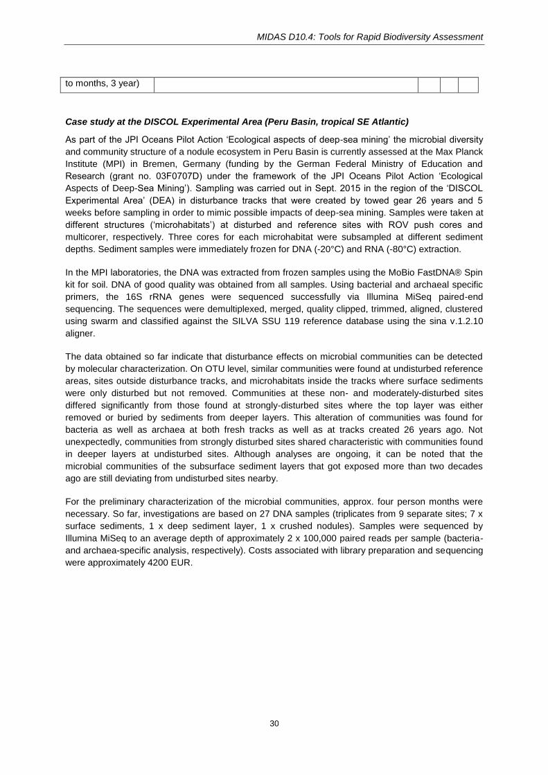
MIDAS D10.4: Tools for Rapid Biodiversity Assessment
30
to months, 3 year)
Case study at the DISCOL Experimental Area (Peru Basin, tropical SE Atlantic)
As part of the JPI Oceans Pilot Action ‘Ecological aspects of deep-sea mining’ the microbial diversity
and community structure of a nodule ecosystem in Peru Basin is currently assessed at the Max Planck
Institute (MPI) in Bremen, Germany (funding by the German Federal Ministry of Education and
Research (grant no. 03F0707D) under the framework of the JPI Oceans Pilot Action ‘Ecological
Aspects of Deep-Sea Mining’). Sampling was carried out in Sept. 2015 in the region of the ‘DISCOL
Experimental Area’ (DEA) in disturbance tracks that were created by towed gear 26 years and 5
weeks before sampling in order to mimic possible impacts of deep-sea mining. Samples were taken at
different structures (‘microhabitats’) at disturbed and reference sites with ROV push cores and
multicorer, respectively. Three cores for each microhabitat were subsampled at different sediment
depths. Sediment samples were immediately frozen for DNA (-20°C) and RNA (-80°C) extraction.
In the MPI laboratories, the DNA was extracted from frozen samples using the MoBio FastDNA® Spin
kit for soil. DNA of good quality was obtained from all samples. Using bacterial and archaeal specific
primers, the 16S rRNA genes were sequenced successfully via Illumina MiSeq paired-end
sequencing. The sequences were demultiplexed, merged, quality clipped, trimmed, aligned, clustered
using swarm and classified against the SILVA SSU 119 reference database using the sina v.1.2.10
aligner.
The data obtained so far indicate that disturbance effects on microbial communities can be detected
by molecular characterization. On OTU level, similar communities were found at undisturbed reference
areas, sites outside disturbance tracks, and microhabitats inside the tracks where surface sediments
were only disturbed but not removed. Communities at these non- and moderately-disturbed sites
differed significantly from those found at strongly-disturbed sites where the top layer was either
removed or buried by sediments from deeper layers. This alteration of communities was found for
bacteria as well as archaea at both fresh tracks as well as at tracks created 26 years ago. Not
unexpectedly, communities from strongly disturbed sites shared characteristic with communities found
in deeper layers at undisturbed sites. Although analyses are ongoing, it can be noted that the
microbial communities of the subsurface sediment layers that got exposed more than two decades
ago are still deviating from undisturbed sites nearby.
For the preliminary characterization of the microbial communities, approx. four person months were
necessary. So far, investigations are based on 27 DNA samples (triplicates from 9 separate sites; 7 x
surface sediments, 1 x deep sediment layer, 1 x crushed nodules). Samples were sequenced by
Illumina MiSeq to an average depth of approximately 2 x 100,000 paired reads per sample (bacteria-
and archaea-specific analysis, respectively). Costs associated with library preparation and sequencing
were approximately 4200 EUR.

MIDAS D10.4: Tools for Rapid Biodiversity Assessment
31
3.2. Meiofaunal biodiversity assessment
Authors: Ann Vanreusel, Ellen Pape, Lara Macheriotou, Lidia Lins, Katja Guilini
Target taxa :
Meiofaunal
invertebrates and
protists
Size groups
Meiofauna
Spatial resolution
Any that may be
addressed by
sampling
Topography
Any as long as sediment samples can
be obtained
Lowest taxonomic
level resolved
Species incl cryptic
species
Surface and
subsurface
Both
Sampling
equipment
Box corer,
Epibenthic
sledge, ROV
push core and
Multicorer
Substrates
Sediments, nodule fields
(Can also be applied to hard
substratum habitats such as off-vents,
crusts, etc.)
Functional group
identification
Based on the
morphology of the
buccal cavity
Temporal
record
Only when
repeated
sampling
Image equipment
Digital images of
each specimen
Ecosystems/target deposits
Mainly sedimentary habitats (i.e.
manganese nodule sites) but any other
is possible if samples may be obtained
Introduction
Similar to macrofauna taxa (see further) there is a need for taxonomic information on deep-sea
meiofaunal organisms from areas targeted for mining. For most meiofauna taxa, including dominant
groups such as nematodes and copepods, there are no dedicated identification guides available
and only few taxonomic papers describe deep-sea species. Consequently, identification of deep-
sea meiofauna is time-consuming and expert-based, whereas cryptic species are possibly
numerous. Therefore the use of metabarcoding for meiofauna biodiversity assessment is promising
for future monitoring approaches but this method is still in a pilot phase (see further). Furthermore,
proper reference DNA sequence databases are missing. To meet the need for fast and more robust
molecular rather than morphological identification approaches in future biodiversity rapid
assessment, both morphological and molecular data on meiofauna species need to be generated
and shared through publically available databases. Environmental sequences (environmental DNA
or eDNA) can then be compared against this reference database of sequences from identified,
vouchered species. Such a comparative analysis allows for the assessment of not only the spatial
distribution range of species but also of the representation of functional groups by linking molecular
sequences to morphospecies.
Protocols (based on nematodes but available for other taxa too)
To sample deep-sea meiofauna, sediment samples are collected using ROV push cores, a
multicorer or a box corer. Sediment samples used for meiofauna barcoding and vouchering are
preserved in DESS (solution of dimethylsulphoxide with EDTA and NaCl salts, cfr. Yoder et al.,
2006). This solution has proven to preserve both the morphology as well as the DNA of marine
nematodes and other meiofauna taxa (Fonseca and Fehlauer-Ale, 2012), making it a suitable
fixative and preservative for studies combining barcoding and morphological identification.
Sediment cores are best processed as quickly as possible after recovery in a temperature-
controlled lab set at in situ temperature to minimize DNA degradation. DESS is added to sediment
samples, using a sample:DESS ratio of 1:1 (or more DESS, if available), immediately following
MIDAS D10.4: Tools for Rapid Biodiversity Assessment
32
recovery on board, after which the sample containers are shaken well to ensure homogeneous
distribution of the liquid preservative. Some researchers replace the DESS after 24 hours to prevent
dilution by water contained within the sediment, though the added value of this approach has so far
not been evidenced. Importantly, a big advantage of using DESS, rather than freezing, is that
samples can be stored at room temperature, significantly simplifying post-sampling logistics.
Preferably within maximum 6 months after sampling, the meiofauna from the DESS-fixed samples
need to be extracted using Ludox centrifugation or a similar extraction technique (Burgess, 2001).
After each of the 3 centrifugation rounds, the supernatant needs to be poured over a 32 µm sieve
and the sieve residue stored in DESS.
Meiofauna specimens need to be hand-picked with a clean tungsten wire needle using a
stereomicroscope. Specimens are cleaned by transferring it several times (number of times
depends on the cleanness of your meiofauna extract) to an embryo dish containing autoclaved Milli-
Q water.
Nematodes are vouchered by transferring them to a drop of autoclaved Milli-Q water on a glass
slide and covering carefully with a glass cover slip. The nematode is then identified down to the
lowest taxonomical level possible (typically genus level) using a microscope. To generate a
voucher, pictures or video sequences are taken of each specimen at the highest microscope
magnification possible of taxonomically important features, such as e.g., the amphid, buccal cavity,
and spicules. After identification, the cover slip is carefully removed, and the nematode is
transferred to an Eppendorf vial containing Worm Lysis Buffer (50 mM KCl, 10 mM Tris pH 8.3, 2.5
mM MgCl2, 0.45 %, NP-40 (octyl phenoxypolyethoxylethanol), 0.45 % Tween 20) for DNA
extraction. The Eppendorf vials with the specimens in worm lysis buffer are best stored frozen at -
20 °C. After thawing, 1 µl of proteinase K is added (10 mg/ml) and mixed by flicking the tube. After
centrifugation (short spin), the samples are incubated at 65° C for 1 h and at 95° C for 10 min and
centrifuged for 1 min at 14000 rpm to pellet the debris down.
In (deep-sea) nematode barcoding studies, 18S and COI marker genes are typically targeted (e.g.,
Bhadury et al., 2011; 2006; Bik et al., 2010). Different primers have been used to amplify 18S and /
or COI depending on the exact fragment one wants to sequence and on the
amplification/sequencing success rate. Following amplification, the quality of the PCR products is
first checked by electrophoresis on a 1 % agarose gel. Only those PCR products that yield a faint or
intense band are further processed. PCR products are cleaned and sent for sequencing to an
external sequencing company. Chromatograms are inspected, edited and aligned using dedicated
software (e.g., open software Unipro UGENE 1.20 (http://ugene.net/)). Because of the risk of wrong
base calls, sequences showing double peaks or extremely low signals should be discarded.
Sequences of COI and 18S can be blasted against respectively NCBI-nr or NCBI-nt for preliminary
determinations of taxonomic identity using respectively blastx and blastn (BLAST 2.2.29+). The
resultant xml-file can be parsed using a custom Biopython script (version 1.63) and sorted for its
specific higher taxa identity. Sequences can be processed and aligned with UGENE (MUSCLE
alignment, available from http://ugene.net/).
References for protocols
Nematodes
Bhadury P, Austen MC, Bilton DT, Lambshead PJD, Rogers AD, Smerdon GR (2006) Development
and evaluation of a DNA-barcoding approach for the rapid identification of nematodes. Marine
Ecology Progress series 320: 1–9.
Bhadury P, Bik H, Lambshead PJD, Austen MC, Smerdon GR, Rogers AD (2011) Molecular
MIDAS D10.4: Tools for Rapid Biodiversity Assessment
33
Diversity of Fungal Phylotypes Co-Amplified Alongside Nematodes from Coastal and Deep-Sea
Marine Environments. PLoS ONE 6: e26445. doi:10.1371/journal.pone.0026445.
Bik HM, Thomas WK, Lunt DH, Lambshead PJD (2010) Low endemism, continued deep-shallow
interchanges, and evidence for cosmopolitan distributions in free-living marine nematodes (order
Enoplida). BMC Evolutionary Biology 10: 389. doi:10.1186/1471-2148-10-389.
Blaxter ML, De Ley P, Garey JR, Liu LX, Scheldeman P, Vierstraete A, Vanfleteren JR, Mackey LY,
Dorris M, Frisse LM, Vida JT, Thomas WK (1998) A molecular evolutionary framework for the
phylum Nematoda. Nature 392: 71-75.
Burgess R (2001) An improved protocol for separating meiofauna from sediments using colloidal
silica sols. Marine Ecology Progress Series 214: 161–165.
Creer S, Fonseca VG, Porazinska DL, Giblin-Davis R, Sung W, Power DM, Packer M, Carvalho
GR, Blaxter ML, Lambshead PJD (2010) Ultrasequencing of the meiofaunal biosphere: practice,
pitfalls and promises. Molecular Ecology 19: 4–20.
Derycke S, Remerie T, Vierstraete A, Backeljau T, Vanfleteren JR, Vincx M, Moens T (2005)
Mitochondrial DNA variation and cryptic speciation within the free-living marine nematode Pellioditis
marina. Marine Ecology Progress Series 300: 91–103. doi:10.3354/meps300091.
Fonseca G, Fehlauer-Ale KH (2012) Three in one: fixing marine nematodes for ecological,
molecular, and morphological studies. Limnology and Oceanography: Methods 10: 516–523.
Yoder M, De Ley IT, King IW, Mundo-Ocampo M, Mann J, Blaxter M, Poiras L, De Ley P (2006)
DESS: a versatile solution for preserving morphology and extractable DNA of nematodes.
Nematology 8: 367–376.
Copepods
Raupach MJ, Barco A, Steinke D, Beermann J, Laakmann S, Mohrbeck I, Neumann H, Kihara TC,
Pointner K, Radulovici A, Segelken-Voigt A, Wesse C, Knebelsberger T (2015) The Application of
DNA Barcodes for the Identification of Marine Crustaceans from the North Sea and Adjacent
Regions. PLoS ONE 10(9): e0139421. doi:10.1371/journal.pone.0139421
Foraminiferans
Pawlowski J, Holzmann M (2014) A Plea for DNA barcoding of Formaminifera. Journal of
Foraminiferal Research 44: 62-67.
SWOT analysis + scoring of criteria
Strengths: The analysis can be applied to any ecosystem / deposit where samples can be
obtained. Any meiofauna taxon can be addressed at many possible levels of taxonomic resolution.
Weaknesses: Rates of success of amplification and sequencing are highly variable depending on
the taxonomic group and typically is between 30 % and 60 %. Gene needs to be selected carefully,
as for example COI does not always amplify or sequence successfully, and in some taxa does not
consistently discriminate between species. Moreover, the barcoding method does not yet allow for
a quantitative analysis of community structure and composition because of the - at present - lower
success rate compared to traditional morphological biodiversity assessment. Finally, it is time- and
labour-consuming and requires a trained taxonomist for vouchering.
Opportunities: By combining morphological identification with barcoding, a reference sequence
database can be built that can be used for identifying environmental sequences when the
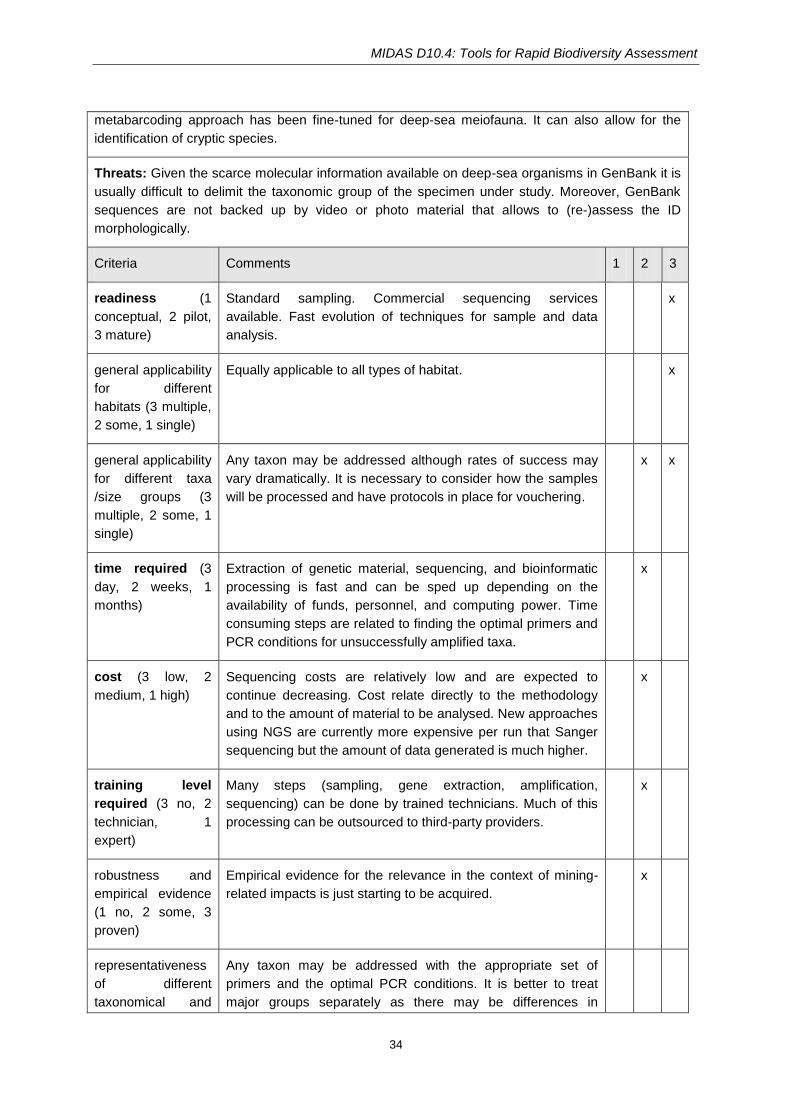
MIDAS D10.4: Tools for Rapid Biodiversity Assessment
34
metabarcoding approach has been fine-tuned for deep-sea meiofauna. It can also allow for the
identification of cryptic species.
Threats: Given the scarce molecular information available on deep-sea organisms in GenBank it is
usually difficult to delimit the taxonomic group of the specimen under study. Moreover, GenBank
sequences are not backed up by video or photo material that allows to (re-)assess the ID
morphologically.
Criteria Comments 1 2 3
readiness (1
conceptual, 2 pilot,
3 mature)
Standard sampling. Commercial sequencing services
available. Fast evolution of techniques for sample and data
analysis.
x
general applicability
for different
habitats (3 multiple,
2 some, 1 single)
Equally applicable to all types of habitat. x
general applicability
for different taxa
/size groups (3
multiple, 2 some, 1
single)
Any taxon may be addressed although rates of success may
vary dramatically. It is necessary to consider how the samples
will be processed and have protocols in place for vouchering.
x x
time required (3
day, 2 weeks, 1
months)
Extraction of genetic material, sequencing, and bioinformatic
processing is fast and can be sped up depending on the
availability of funds, personnel, and computing power. Time
consuming steps are related to finding the optimal primers and
PCR conditions for unsuccessfully amplified taxa.
x
cost (3 low, 2
medium, 1 high)
Sequencing costs are relatively low and are expected to
continue decreasing. Cost relate directly to the methodology
and to the amount of material to be analysed. New approaches
using NGS are currently more expensive per run that Sanger
sequencing but the amount of data generated is much higher.
x
training level
required (3 no, 2
technician, 1
expert)
Many steps (sampling, gene extraction, amplification,
sequencing) can be done by trained technicians. Much of this
processing can be outsourced to third-party providers.
x
robustness and
empirical evidence
(1 no, 2 some, 3
proven)
Empirical evidence for the relevance in the context of mining-
related impacts is just starting to be acquired.
x
representativeness
of different
taxonomical and
Any taxon may be addressed with the appropriate set of
primers and the optimal PCR conditions. It is better to treat
major groups separately as there may be differences in

MIDAS D10.4: Tools for Rapid Biodiversity Assessment
35
functional groups (1
single, 2 multiple, 3
all)
developing successful primers.
taxonomic
resolution (1
highest: phyla to
order;2 medium:
family to genus;
lowest: 3 species or
OTU)
Operational taxonomic units – nominally species level. x
spatial coverage
(1 cm², 2 m², 3 km²)
Analyses reflect the sampling regime so it can vary from
samples take within 10s of meters of each other to comparison
of sample sets in different areas.
x x
Temporal
coverage (1
snapshot, 2 weeks
to months, 3 year)
Analyses are based on samples collected in different years. x
Illustration from a MIDAS case study
Barcoding of free-living marine nematodes from the Clarion-Clipperton Fracture Zone (CCFZ) is
currently underway at Ghent University using the protocol described above. These samples were
collected at abyssal depths from several sites hundreds of km's apart. The chosen primers target the
18S and COI molecular markers. Extraction of DNA has been straightforward and successful
throughout. Subsequent PCR using the aforementioned primers illustrates one of barcoding’s
weaknesses, i.e. the somewhat unpredictable amplification success of the chosen markers. Results
thus far indicate a significantly higher success rate of the 18S marker over COI across all processed
taxa (90 % versus 62 %, respectively). However, troubleshooting and PCR protocol optimization can
aid in maximizing positive amplification. High quality sequence data become available typically within
2-3 days with rapid bioinformatic analyses providing phylogenetic and biogeographic data that are
intuitively visualized in the form of cladograms. Despite the small number of analyzed samples thus
far, the barcoding method has been successful at providing preliminary insights regarding the
nematode community composition in the CCFZ as well as tentative population connectivity patterns.

MIDAS D10.4: Tools for Rapid Biodiversity Assessment
36
3.3. Benthic macrofaunal biodiversity assessment
Authors: Sergi Taboada, Gordon Paterson, Adrian Glover, Lenaick Menot, Thomas Dahlgren
Target taxa :
Macrofaunal
invertebrates
Size groups
Macrofauna
Spatial resolution
Any that may be
addressed by
sampling
Topography
Any as long as samples can be
obtained
Lowest taxonomic
level resolved
Species (incl.
cryptic species)
Surface/
Subsurface
Both
Sampling
equipment
Box corer,
Epibenthic
sledge, ROV
Substrates
Sediment, nodule fields
(Can also be applied to hard
substratum habitats such as off-vents,
crusts, etc.)
Functional group
identification
Only based on
morphology
Temporal
record
Only when
sampling is
repeated
Image equipment
Digital images of
each
morphotype/
specimen
Ecosystems/target deposits
Mainly sedimentary habitats (i.e.,
Manganese nodule sites) but any other
is possible if samples may be obtained
Introduction
There is an urgent need to provide accurate and widely-available taxonomic information on the
organisms to be found in the CCFZ (the approach could be adapted for other deep-sea habitats
such as vent fields and crusts). Despite decades of investigation, there are no identification guides,
few taxonomic papers describing species from the CCFZ and therefore little or only vague ideas on
the distribution of organisms across this area.
The challenge in the CCFZ is particularly acute as this is the area of focus for several nations
exploring the potential mineral resources to be found in this abyssal region. The CCFZ is
fragmented into a number of licensed exploration areas allocated to different nations. Each
nation/contractor is required to undertake environmental assessments and develop an
environmental baseline, prior to any exploitation of the licensed areas they hold. Despite these
regulations very little taxonomic information has emerged. Each contractor employs their own
specialists and such work is often focused on producing quantitative biodiversity assessments.
There are resource and time constraints on the work being done and so identifications often remain
at the level of sp.1 or sp.A. Increased collaborations and exchange of information would allow for
the recognition that one contractor’s sp.1 is the same as another’s sp.A.
Yet to be able to assess the threat of extinction due to mining, it is vital to understand the
distribution of species across the whole region not just in one claim area, and to have an appreciate
on the connectivity between different populations of the species.
To achieve this fundamental but critical goal, taxonomic information needs to be generated quickly
and made available. Taxonomic studies are perceived to be time consuming. Indeed, it can take
time to produce good taxonomic research output and this has contributed to a global challenge to
be able to assess the biodiversity of threatened habitats before they are altered irreversibly.
However, the rise of molecular protocols and the decreasing costs associated with methods such as
DNA-barcoding offer an opportunity to generate the taxonomic information in the time frame
needed. The methods described below are based on Glover et al. (2015), Janssen et al. (2015) and
Riehl et al. (2014). These approaches aim to combine traditional morphological taxonomy with
MIDAS D10.4: Tools for Rapid Biodiversity Assessment
37
DNA-barcoding or similar molecular approaches but to make available the identifications within a
reasonable timeframe from the initial collection. Critical to this approach is to link the morphological
data with the molecular because currently there are few sequences available which can be related
to existing species. This taxonomic baseline is an essential step towards developing a monitoring
approach which, by only using molecular methods based on a solid taxonomy of the organisms
present, can allow rapid monitoring assessment of the environment.
So it is essential to invest in the necessary ship-board effort needed to live sort material as it is
collected. The protocols here focus on getting good material and can be considered a qualitative
approach rather than the more ecologically focused quantitative surveys that have characterised
abyssal studies for the previous two decades. The focus is on getting good specimens, imaged and
then processed for molecular studies. Keeping the material as cold as possible is essential at all
stages of the ship-board processing. The chances of obtaining successful DNA sequences
increases dramatically by establishing a cold-chain from the moment the sample comes on board to
when the specimens are put into preserving fluid. It is also necessary that good data management
protocols are developed to keep track of the specimen and related information such as its image,
bar-code, etc. (see Glover et al., 2015).
The final step is to publish as quickly as possible on the taxa which have been bar-coded in this
way. In Glover et al. (2016), data from echinoderms was made available using on-line data journals
such as the Biodiversity Data Journal. In this way other teams can access the information and relate
their morphological specimens or sequences to what was found during the ABYSSLINE surveys. In
this way a consistent taxonomy can be developed and a greater understanding of the distribution of
the species concerned can be gained. This in turn allows a more accurate assessment of the risks
to species extinction from mining activities.
Protocols including sampling, data collection and data processing
(based on the protocols by Glover et al., 2015; Janssen et al., 2015; Riehl et al., 2014).
Sampling
Sampling of sediment and hard substrates (e.g., polymetallic nodules) is carried out with standard
gear (e.g., Boxcore, Multicorer). The cold-chain method is essential to preserving high-quality
individual specimens to be used for molecular analyses. To this end, a system of pumps and cold-
water reservoirs needs to be set up in order to keep specimens cold (target temperature of 2˚C)
whilst they were being sieved (using a 300 μm sieve) and live sorted. Once sorted, animals are
photographed alive, preserved in chilled 80 % ethanol (and occasionally RNAlater), and
immediately stored at -20°C until sample processing. Preservation in 80 % ethanol in soft-bodied
organisms (e.g., annelid polychaetes) allows for a combined molecular and morphological
approach. DNA from samples is extracted using conventional extraction kits. 80 % ETOH has been
shown to be effective in preserving DNA for future studies. The success rate for molecular analyses
reducing the concentration from absolute alcohol appears to be unaffected.
See Glover et al. (2015) and Riehl et al. (2014) for details on the methods used onboard the ship for
sorting and processing different taxa and from different sampling gears.
Sample and data analysis
About 1800 bp of 18S, 800 bp of 28S (D1-D2 region), 450 bp of 16S, and 650 bp of cytochrome c
oxidase subunit I (COI) are amplified using either published or newly-designed primers (depending
on the taxa of choice). Amplification is carried out using a mixture of the primers, a Taq DNA
MIDAS D10.4: Tools for Rapid Biodiversity Assessment
38
polymerase and DNA template from the sample under study (e.g., 1 μL of each primer (10 μM), 2
μL DNA template and 21 μL of Red Taq DNA Polymerase 1.1x MasterMix (VWR) in a mixture of
total 25 μL). The PCR amplification profile consists of initial denaturation at 95 °C for 5 min, 35
cycles of denaturation at 94 °C for 45 s, annealing at 55 °C for 45 s, extension at 72 °C for 2 min,
and a final extension at 72 °C for 10 min. Typically, PCR products are purified using Millipore
Multiscreen 96-well PCR Purification System, and sequencing is performed on an ABI 3730XL DNA
Analyser (Applied Biosystems) at a sequencing facility, using the same primers as in the PCR
reactions.
For isopods Riehl et al. (2014) suggest the following approach. The sequences were amplified in
partially overlapping fragments using three primer pairs (18 A1 and 700 R; 400 F and 1155 R; 1000
F and 1800). The PCR profile comprised an initial denaturation at 95 °C (10 min), followed by 36
cycles of denaturation at 94 °C (30 s), annealing at 54 °C (45 s) and extension at 72 °C (3 min 12 s)
followed by a final extension at 72 °C (10 min). Cycle sequencing was performed using the same
primers as used for PCR.
Once sequences are obtained, overlapping fragments are merged into consensus sequences using
a software platform for the organization and analysis of sequence data e.g., Geneious (Kearse et
al., 2012) and aligned using MAFFT (Katoh et al., 2002) for 18S, 28S and 16S, and MUSCLE
(Edgar, 2004) for COI, both programs used as plugins in Geneious, with default settings.
Sequences obtained are blasted with sequences deposited in GenBank. Bayesian phylogenetic
analyses (BA) are conducted with MrBayes 3.1.2 (Ronquist and Huelsenbeck, 2003) following
standard methods for phylogenetic inference, and the phylogenetic trees produced are used to
identify consistent monophyletic clades of specimens. Statistically well-supported clades where
“within-clade” sequence variation is lower than “between-clade” variation are hypothesised as
operational taxonomic units (OTUs). Finally, a combination of the molecular and morphological
information is used to establish the characteristic features of a given OTU.
References for protocols
Edgar RC (2004) Muscle: Multiple sequence alignment with high accuracy and high throughput.
Nucleic Acids Research 32: 1792–1797.
Glover AG, Dahlgren TG, Wiklund H, Mohrbeck I, Smith CR (2015) An End-to-End DNA Taxonomy
Methodology for Benthic Biodiversity Survey in the Clarion-Clipperton Zone, Central Pacific Abyss.
Journal of Marine Science and Engineering 4(2). doi:10.3390/jmse4010002.
Glover A, Wiklund H, Rabone M, Amon D, Smith C, O'hara T, Mah C, Dahlgren T (2016) Abyssal
fauna of the UK-1 polymetallic nodule exploration claim, Clarion-Clipperton Zone, central Pacific
Ocean: Echinodermata. Biodiversity Data Journal 4: e7251 - e7251. doi: 10.3897/BDJ.4.e7251.
Janssen A, Kaiser S, Meißner K, Brenke N, Menot L, Martínez Arbizu P (2015) A Reverse
Taxonomic Approach to Assess Macrofaunal Distribution Patterns in Abyssal Pacific Polymetallic
Nodule Fields. PLoS ONE 10(2): e0117790. doi:10.1371/journal.pone.0117790.
Katoh K, Misawa K, Kuma K, Miyata T (2002) Mafft: A novel method for rapid multiple sequence
alignment based on fast fourier transform. Nucleic Acids Research 30: 3059–3066.
Kearse M, Moir R, Wilson A, Stones-Havas S, Cheung M, Sturrock S, Buxton S, Cooper A,
Markowitz S, Duran C, et al. (2012) Geneious basic: An integrated and extendable desktop software
platform for the organization and analysis of sequence data. Bioinformatics 28: 1647–1649.
Riehl T, Brenke N, Brix, S, Driskell A, Kaiser S, Brandt A (2014) Field and Laboratory Methods for
DNA Studies on Deep-sea Isopod Crustaceans. Polish Polar Research 35(2): 203–224.

MIDAS D10.4: Tools for Rapid Biodiversity Assessment
39
Ronquist F, Huelsenbeck JP (2003) Mrbayes 3: Bayesian phylogenetic inference under mixed
models. Bioinformatics 19: 1572–1574.
SWOT analysis + scoring of criteria
Strengths: The analysis can be applied to any ecosystem / deposit where samples can be
obtained. Any taxon of the macrofaunal community can be addressed at many possible levels of
taxonomic resolution.
Weaknesses: Rates of success of amplification and sequencing are highly variable depending on
the taxonomic group and are typically around 50 %. There is also some disagreement as to what
barcodes mean. It is assumed that species-level discrimination is being undertaken but this is not
always the case. Care has to be taken in the selection of the gene being used as the barcode as for
example CO1 does not always work and in some taxa does not consistently discriminate at the
species level.
The method does not allow for a quantitative analysis of community structure unless all individuals
from a quantitative sample are processed.
On a practical level the approach needs a dedicated team of at least three preferably four to five to
operate, with at least two persons processing material that has been sorted. The more people the
faster the sample can be dealt with which reduces the backlog of material that could build up.
Opportunities: Methods evolve fast, resolution and discrimination improve and associated costs
decrease. If the protocols are robustly adopted it is possible to produce good reproducible and
publishable data within 12 months of collecting. Thus responding to the need for biodiversity
information within a relatively short timeframe.
Threats: Given the scarce molecular information available of deep-sea organisms in GenBank it is
usually difficult to delimit the taxonomic group of the specimen under study. In mixed discipline
cruises there is pressure on berths which can restrict the biology team. Recent taxonomic
workshops sponsored by the ISA have produced recommendations that biology focused cruises are
essential if the taxonomic baseline of the Area is to be improved. There is also the issue that
scientific teams under pressure to produce results within short time frames (usually associated with
environmental impact assessments) will see molecular analyses as a shortcut and switch to
barcoding without developing the morphological link. The area of molecular analyses is a fast
developing one. At one end of the spectrum are mature and robust approaches such as barcoding
while at the other new and developing technologies, such as transcriptomics, are emerging. The
issue for environmental baseline and monitoring studies is the fear that one method will supersede
another but that there will be a lack of continuity between them, rendering previous studies
irrelevant or questionable.
Criteria Comments 1 2 3
readiness (1
conceptual, 2 pilot,
3 mature)
Standard sampling. Commercial sequencing services
available. Fast evolution of techniques for sample and data
analysis.
x
general applicability
for different habitats
(3 multiple, 2 some,
Equally applicable for any habitat. x

MIDAS D10.4: Tools for Rapid Biodiversity Assessment
40
1 single)
general applicability
for different taxa
/size groups (3
multiple, 2 some, 1
single)
Any taxon may be addressed although rates of success may
vary dramatically. It is necessary to consider how the samples
will be processed and have protocols in place to sub-sample
tissue for molecular analyses.
x
time required (3
day, 2 weeks, 1
months)
Extraction of genetic material, sequencing, and bioinformatic
processing is fast and can be sped up depending on the
availability of funds, personnel, and computing power. Time
consuming steps are related to finding the optimal PCR
conditions for unsuccessfully amplified taxa.
x
cost (3 low, 2
medium, 1 high)
Sequencing costs are relatively low and are expected to
continue decreasing. Cost relate directly to the methodology
and to the amount of material to be analysed. New
approaches using NGS are currently more expensive per run
that Sanger sequencing but the amount of data generated is
much higher.
x
training level
required (3 no, 2
technician, 1 expert)
Many steps (sampling, gene extraction, amplification,
sequencing) can be done by trained technicians. Much of this
processing can be outsourced to third party providers. Even
phylogenetic analyses do not require a high level of expertise.
x
robustness and
empirical evidence
(1 no, 2 some, 3
proven)
Empirical evidence for the relevance in the context of mining-
related impacts is just starting to be acquired.
x
representativeness
of different
taxonomical and
functional groups
(1single, 2 multiple,
3 all)
Any taxon may be addressed with the appropriate set of
primers and the optimal PCR conditions. It is better to treat
major groups separately as there may be differences in
developing successful primers.
x
taxonomic
resolution (1
highest: phyla to
order;2 medium:
family to genus;
lowest: 3 species or
OTU)
Operational taxonomic units – nominally species level. x
spatial coverage
(1 cm², 2 m², 3 km²)
Analyses reflect the sampling regime so it can vary from
samples take within 10s of meters of each other to
comparison of sample sets in different areas.
x x

MIDAS D10.4: Tools for Rapid Biodiversity Assessment
41
Temporal
coverage (1
snapshot, 2 weeks
to months, 3 year)
Analyses are based on samples collected through different
years.
x
Illustration from a MIDAS case study
MIDAS Cruise JC120 to CCFZ July 2015. During this cruise the protocol used in the ABYSSLINE
project outlined by Glover et al. (2015) was used successfully. An example of processing material from
a box-core sample summarizes the main activities and results.
- Samples collected, once on deck box core surface sample photographed after surface water
carefully drained off through a 300 µm sieve and the residue retained in cold seawater for
future analyses.
- Large volumes of cold sea-water (2-4 ºC) already cooled to use for sorting.
- Box core processed with sediment and nodules being separated. Box cores sliced with the top
0-2 cm being taken and held in cold room awaiting sieving and live sorting.
- Nodules and mud analysed separately in the cold room (4 ºC) in order to preserve material as
well as possible. Nodules removed and examined for encrusting and epifauna. Fauna
removed, photographed and preserved in cold 80 % ETOH.
- Mud sieved through 300 µm: 0-2 fraction in box core (+ 0-10 fraction in megacore).
- Specimens sorted from sieve residue, then photographed live in the wet lab prior to
preservation in cold 80 % ETOH. Each specimen given unique identification number and
details entered into a specimen spreadsheet.
- In the NHM: extraction of DNA, and amplification and sequencing of selected genes such as
the COI (barcode). Selected species with several individuals from different stations used to
construct haplotype networks to infer gene flow between sites.
- Total of 524 individuals collected, photographed and preserved.
11 phyla including: Arthropoda, Porifera, Annelida, Cnidaria, Mollusca, and Echinodermata as the
most represented ones, but also Nematoda, Chaetognata, Bryozoa, Platyhelminthes, and
Brachiopoda.
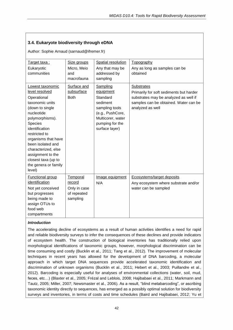
MIDAS D10.4: Tools for Rapid Biodiversity Assessment
42
3.4. Eukaryote biodiversity through eDNA
Author: Sophie Arnaud ([email protected])
Target taxa :
Eukaryotic
communities
Size groups
Micro, Meio
and
macrofauna
Spatial resolution
Any that may be
addressed by
sampling
Topography
Any as long as samples can be
obtained
Lowest taxonomic
level resolved
Operational
taxonomic units
(down to single
nucleotide
polymorphisms).
Species
identification
restricted to
organisms that have
been isolated and
characterized, else
assignment to the
closest taxa (up to
the genera or family
level)
Surface and
subsurface
Both
Sampling
equipment
Standard
sediment
sampling tools
(e.g., PushCore,
Multicorer, water
pumping for the
surface layer)
Substrates
Primarily for soft sediments but harder
substrates may be analyzed as well if
samples can be obtained. Water can be
analyzed as well
Functional group
identification
Not yet conceived
but progresses
being made to
assign OTUs to
food web
compartments
Temporal
record
Only in case
of repeated
sampling
Image equipment
N/A
Ecosystems/target deposits
Any ecosystem where substrate and/or
water can be sampled
Introduction
The accelerating decline of ecosystems as a result of human activities identifies a need for rapid
and reliable biodiversity surveys to infer the consequences of these declines and provide indicators
of ecosystem health. The construction of biological inventories has traditionally relied upon
morphological identifications of taxonomic groups, however, morphological discrimination can be
time consuming and costly (Bucklin et al., 2011; Tang et al., 2012). The improvement of molecular
techniques in recent years has allowed for the development of DNA barcoding, a molecular
approach in which target DNA sequences provide accelerated taxonomic identification and
discrimination of unknown organisms (Bucklin et al., 2011; Hebert et al., 2003; Puillandre et al.,
2012). Barcoding is especially useful for analyses of environmental collections (water, soil, mud,
feces, etc…) (Blaxter et al., 2005; Frézal and Leblois, 2008; Hajibabaei et al., 2011; Markmann and
Tautz, 2005; Miller, 2007; Newsmaster et al., 2006). As a result, “blind metabarcoding”, or ascribing
taxonomic identity directly to sequences, has emerged as a possibly optimal solution for biodiversity
surveys and inventories, in terms of costs and time schedules (Baird and Hajibabaei, 2012; Yu et

MIDAS D10.4: Tools for Rapid Biodiversity Assessment
43
al., 2012).
Morphological and molecular approaches have long been considered complementary (Barber and
Boyce, 2006; Ji et al., 2013), however, many studies performed have demonstrated increased time
efficiency of molecular techniques, in which a single barcoding gene was used (Creer et al., 2010;
Fonseca et al., 2010; Ji et al., 2013; Lindeque et al., 2013; Porazinska et al., 2010).
Baird DJ, Hajibabaei M (2012) Biomonitoring 2.0: a new paradigm in ecosystem assessment made possible by next-generation DNA sequencing. Molecular Ecology 21(8): 2039-2044.
Barber P, Boyce SL (2006) Estimating diversity of Indo-Pacific coral reef stomatopods through DNA barcoding of stomatopod larvae. Proceedings of the Royal Society B 273: 2053–2061. doi:10.1098/rspb.2006.3540.
Blaxter M, Mann J, Chapman T, Thomas F, Whitton C, Floyd R, Abebe E (2005) Defining operational taxonomic units using DNA barcode data. Phil. Trans. R. Soc. B 360: 1935-1943.
Bucklin A, Steinke D, Blanco–Bercial L (2011) DNA Barcoding of Marine Metazoa. Annual Review of Marine Science 3: 18.1–18.38.
Creer S, Fonseca VG, Porazinska DL, Giblin-Davies RM, Sung W, Power DM, Packer M, Carvalho GR, Blaxter ML, Lambshead PJD, Thomas WK (2010) Ultrasequencing of the meiofaunal biosphere: practice, pitfalls and promises. Molecular Ecology 19: (Suppl. 1) 4-20.
Fonseca VG, Carvalho GR, Sung W, Johnson HF, Power DM, Neill SP, Packer M, Blaxter ML, Lambshead PJD, Thomas WK, Creer S (2010) Second-generation environmental sequencing unmasks marine metazoan biodiversity. Nat Commun 1: 98.
Frézal L, Leblois R (2008) Four years of DNA barcoding: Current advances and prospects. Infection, Genetics and Evolution 8: 727-736.
Hajibabaei M, Shokralla S, Zhou X, Singer GAC, Baird DJ (2011) Environmental barcoding: a next-generation sequencing approach for biomonitoring applications using river benthos. PLoS ONE 6(4): e17497. doi:10.1371/journal.pone.0017497.
Hebert PDN, Cywinska A, Ball SL, deWaard JR (2003) Biological identifications through DNA barcodes. Proc. R. Soc. Lond. B 270: 313-321.
Ji Y, Ashton L, Pedley SM, Edwards DP, Tang Y, Nakamura A, Kitching R, Dolman PM, Woodcock P, Edwards FA, Larsen TH, Hsu WW, Benedick S, Hamer KC, Wilcove DS, Bruce C, Wang X, Levi T, Lott M, Emerson BC, Yu DW (2013) Reliable, verifiable and efficient monitoring of biodiversity via metabarcoding. Ecology Letters 16(10): 1245-1257. doi:10.1111/ele.12162.
Lindeque PK, Parry HE, Harmer RA, Somerfield PJ, Atkinson A (2013) Next Generation Sequencing Reveals the Hidden Diversity of Zooplankton Assemblages. PLoS ONE 8(11): e81327. doi:10.1371/journal.pone.0081327.
Markmann M, Tautz D (2005) Reverse taxonomy: an approach towards determining the diversity of meiobenthic organisms based on ribosomal RNA signature sequences. Phil. Trans. R. Soc. Lond. B 360: 1917-1924.
Miller SE (2007) DNA barcoding and the renaissance of taxonomy. PNAS 104(12): 4775-4776. doi:10.1073/pnas.0700466104.
Newmaster SG, Fazekas AJ, Ragupathy, S (2006) ‘DNA barcoding in the land plants: evaluation of rbcL in a multigene tiered approach’. Canadian Journal of Botany 84: 335–341.

MIDAS D10.4: Tools for Rapid Biodiversity Assessment
44
Porazinska DL, Sung WY, Giblin-Davis RM, Thomas WK (2010) Reproducibility of read numbers in high-throughput sequencing analysis of nematode community composition and structure. Molecular Ecology Resources 10: 666-676.
Puillandre N, Lambert A, Brouillet S, Achaz G (2012) ABGD, Automatic Barcode Gap Discovery for primary species delimitation. Molecular Ecology 21(8): 1864-1877.
Tang CQ, Leasi F, Obertegger U, Kieneke A, Barraclough TG, Fontaneto D (2012) The widely used small subunit 18S rDNA molecule greatly underestimates true diversity in biodiversity surveys of the meiofauna. PNAS 109(40): 16208-16212.
Yu DW, Ji Y, Emerson BC, Wang X, Ye C, Yang C, Ding Z (2012) Biodiversity soup: metabarcoding of arthropods for rapid biodiversity assessment and biomonitoring. Methods in Ecology and Evolution 3(4): 613-623.
Protocols including sampling, data collection and data processing
Sampling
Sampling of sediment is carried out with standard gear (e.g., ROV Push Core, Multicorer). Samples
are stored frozen (best at – 80 °C) with or without prior treatment with storage reagent (e.g.,
RNAlater). Sampling of hard substrates or bottom waters requires other instruments (e.g., grabs,
CTD/Rosette samplers, Niskin,…) and additional sample preparation steps (sieving, filtering). Gene
material is extracted from the samples using a combination of physical and chemical methods by
means of routine procedures that typically involve commercially available kits.
Sample and data analysis
A suite of analytical methods targeting DNA for metabarcoding now starts to be available and
performed by dedicated commercial laboratories, mostly targeting 18S, 16S and ITS genes
sequenced using high throughput methods. However, the gene mostly used for metabarcoding of
eukaryotes, Cytochrome Oxidase 1, is currently not proposed routinely by the platforms due to the
difficulties in designing primers allowing the amplification of 1) a large set of taxa, and 2) a
sequence size corresponding to the now decreased size imposed by HiSeq or even MiSeq
sequencing compared to the declining 454 methodology.
Following quality control, statistical analyses are performed in order to classify genes and to deduce
taxonomy, functional gene repertoire and potential and expressed metabolic functions.
References for protocols
Boyer F, Mercier C, Bonin A, Le Bras Y, Taberlet P, Coissac E (2016) OBITOOLS: a UNIX-inspired
software package for DNA metabarcoding. Molecular Ecology Resources 16(1): 176-182.
Caporaso JG, Kuczynski J, Stombaugh J, Bittinger K, Bushman FD, Costello EK, Fierer N, Pena
AG, Goodrich JK, Gordon JI, et al. (2010) QIIME allows analysis of high-throughput community
sequencing data. Nat Methods 7(5): 335-336.
Cowart DA, Pinheiro M, Mouchel O, Maguer M, Grall J, Miné J, Arnaud-Haond S (2015)
Metabarcoding Is Powerful yet Still Blind: A Comparative Analysis of Morphological and Molecular
Surveys of Seagrass Communities. PLoS ONE 10(2): e0117562.
doi:10.1371/journal.pone.0117562.
Fosso B, Santamaria M, Marzano M, Alonso-Alemany D, Valiente G, Donvito G, Monaco A,
Notarangelo P, Pesole G (2015) BioMaS: a modular pipeline for Bioinformatic analysis of

MIDAS D10.4: Tools for Rapid Biodiversity Assessment
45
Metagenomic AmpliconS. BMC Bioinformatics 16(1): 1-11.
Guardiola M, Uriz MJ, Taberlet P, Coissac E, Wangensteen OS, Turon X (2015) Deep-Sea, Deep-
Sequencing: Metabarcoding Extracellular DNA from Sediments of Marine Canyons. PLoS ONE
10(10): e0139633. doi:10.1371/journal.pone.0139633.
Ji Y, Ashton L, Pedley SM, Edwards DP, Tang Y, Nakamura A, Kitching R, Dolman PM, Woodcock P, Edwards FA, Larsen TH, Hsu WW, Benedick S, Hamer KC, Wilcove DS, Bruce C, Wang X, Levi T, Lott M, Emerson BC, Yu DW (2013) Reliable, verifiable and efficient monitoring of biodiversity via metabarcoding. Ecology Letters 16(10): 1245-1257. doi:10.1111/ele.12162.
Mahe F, Rognes T, Quince C, de Vargas C, Dunthorn M (2014) Swarm: robust and fast clustering
method for amplicon-based studies. PeerJ, 2.
Mahe F, Rognes T, Quince C, de Vargas C, Dunthorn M (2015) Swarm v2: highly-scalable and
high-resolution amplicon clustering. PeerJ, 3.
Mendoza MLZ, Sicheritz-Ponten T, Gilbert MTP (2015) Environmental genes and genomes:
understanding the differences and challenges in the approaches and software for their analyses.
Brief Bioinform 16(5): 745-758.
Schloss PD, Westcott SL, Ryabin T, Hall JR, Hartmann M, Hollister EB, Lesniewski RA, Oakley BB,
Parks DH, Robinson CJ, et al. ( Introducing mothur: Open-Source, Platform-Independent,
Community-Supported Software for Describing and Comparing Microbial Communities. Applied and
Environmental Microbiology 2009, 75(23):7537-7541.
Westcott SL, Schloss PD (2015) De novo clustering methods outperform reference-based methods
for assigning 16S rRNA gene sequences to operational taxonomic units. PeerJ 3: e1487.
SWOT analysis + scoring of criteria
Strengths: Similarly to the microbial analysis, the analysis can be applied to any ecosystem /
deposit where samples can be obtained. Any taxon can be addressed at different possible
taxonomic resolution. Allows saving a lot of time compared to morphological approach and provides
with more comprehensive biodiversity assessment. Provides an objective assessment that can be
standardized so comparison is rather reliable if persons performing the analysis change (compared
to the subjective nature of morphological taxonomy and the risks of significant changes when
changing observer).
Weaknesses: There is 1) a need for more pilot studies to identify more universal primers or more
complete set of primers allowing for a comprehensive capture of the taxonomic diversity present in
a given sample 2) a need for an improvement of extent and curation of reference databases.
Similarly to microbial analysis, but even more acute due to a more recent development:
standardization of target genome regions, analytical methods, and data analysis workflows are not
yet achieved. Part of the workflow requires experts, for the definition of primers and the
bioinformatics analysis. Individual analyses are snapshots in space and time only. Relevance in the
context of (mining) impacts is not fully assessed yet.
The assessment is qualitative; the abundance of each taxonomic unit cannot be quantified with
such methods.
The remanescence time of DNA once extracellular in the sediment and water is not exactly known
but strongly suspected to reach very long time, in particular in anoxic sediment and at low
temperature. As consequence, the method does not provide a picture of what is there but rather
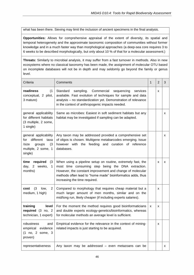
MIDAS D10.4: Tools for Rapid Biodiversity Assessment
46
what has been there. Sieving may limit the inclusion of ancient specimens in the final analysis.
Opportunities: Allows for comprehensive appraisal of the extent of diversity, its spatial and
temporal heterogeneity and the approximate taxonomic composition of communities without former
knowledge and in a much faster way than morphological approaches (a deep-sea core requires 3 to
6 weeks to be described morphologically, but only about 10 % of that for a molecular assessment.)
Threats: Similarly to microbial analysis, it may suffer from a fast turnover in methods. Also in new
ecosystems where no classical taxonomy has been made, the assignment of molecular OTU based
on incomplete databases will not be in depth and may seldomly go beyond the family or genus
level.
Criteria Comments 1 2 3
readiness (1
conceptual, 2 pilot,
3 mature)
Standard sampling. Commercial sequencing services
available. Fast evolution of techniques for sample and data
analysis – no standardization yet. Demonstration of relevance
in the context of anthropogenic impacts needed.
x
general applicability
for different habitats
(3 multiple, 2 some,
1 single)
Same as microbes: Easiest in soft sediment habitats but any
habitat may be investigated if sampling can be adapted.
x
general applicability
for different taxa
/size groups (3
multiple, 2 some, 1
single)
Any taxon may be addressed provided a comprehensive set
of oligos is chosen. Multigene metabarcodes emerging. Issue
however with the feeding and curation of reference
databases.
x
time required (3
day, 2 weeks, 1
months)
When using a pipeline setup on routine, extremely fast, the
most time consuming step being the DNA extraction.
However, the constant improvement and change of molecular
methods often lead to “home made” bioinformatics adds, thus
increasing the time required.
x x
cost (3 low, 2
medium, 1 high)
Compared to morphology that requires cheap material but a
much larger amount of men months, similar and on the
mid/long run, likely cheaper (if including experts salaries).
x
training level
required (3 no, 2
technician, 1 expert)
For the moment the method requires good bioinformaticians
and double experts ecology-genetics/bioinformatics, whereas
for molecular methods an average level is sufficient.
x x
robustness and
empirical evidence
(1 no, 2 some, 3
proven)
Empirical evidence for the relevance in the context of mining-
related impacts is just starting to be acquired.
x
representativeness Any taxon may be addressed – even metazoans can be x

MIDAS D10.4: Tools for Rapid Biodiversity Assessment
47
of different
taxonomical and
functional groups (1
single, 2 multiple, 3
all)
identified with similar techniques as long as a comprehensive
set of primers is defined.
taxonomic
resolution (1
highest: phyla to
order;2 medium:
family to genus;
lowest: 3 species or
OTU)
Operational taxonomic units only, i.e. numbers.
The reliability of their taxonomic assignment depends on the
amount of species present in the studied community that were
already described through a double approach (morphology,
molecular barcode) and posted in the reference databases. A
pilot double approach molecular-morphological is advised
when feasible in order to feed databases, thus increasing the
amount of assignments up to the species level.
x
spatial coverage
(1 cm², 2 m², 3 km²)
Sampling of sediment limited to several cm2 but with
replicates extending to m2, water a little more representative
(but more admixed with larger scales depending on the water
motion). Requires replicates and nested sampling. Allows
assessing spatial heterogeneity with a good sampling design
and a temporal approach.
x
Temporal
coverage (1
snapshot, 2 weeks
to months, 3 year)
Repeating the analysis implies repeating sampling, thus
cruises. Everything else is just one snapshot. However, this
snapshot may integrate taxa that have been present several
days/weeks ago (see weaknesses).
x
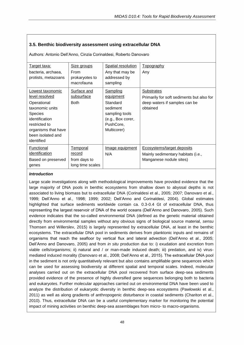
MIDAS D10.4: Tools for Rapid Biodiversity Assessment
48
3.5. Benthic biodiversity assessment using extracellular DNA
Authors: Antonio Dell’Anno, Cinzia Corinaldesi, Roberto Danovaro
Target taxa:
bacteria, archaea,
protists, metazoans
Size groups
From
prokaryotes to
macrofauna
Spatial resolution
Any that may be
addressed by
sampling
Topography
Any
Lowest taxonomic
level resolved
Operational
taxonomic units
Species
identification
restricted to
organisms that have
been isolated and
identified
Surface and
subsurface
Both
Sampling
equipment
Standard
sediment
sampling tools
(e.g., Box corer,
PushCore,
Multicorer)
Substrates
Primarily for soft sediments but also for
deep waters if samples can be
obtained
Functional
identification
Based on preserved
genes
Temporal
record
from days to
long time scales
Image equipment
N/A
Ecosystems/target deposits
Mainly sedimentary habitats (i.e.,
Manganese nodule sites)
Introduction
Large scale investigations along with methodological improvements have provided evidence that the
large majority of DNA pools in benthic ecosystems from shallow down to abyssal depths is not
associated to living biomass but to extracellular DNA (Corinaldesi et al., 2005; 2007; Danovaro et al.,
1999; Dell’Anno et al., 1998; 1999; 2002; Dell’Anno and Corinaldesi, 2004). Global estimates
highlighted that surface sediments worldwide contain ca. 0.3-0.4 Gt of extracellular DNA, thus
representing the largest reservoir of DNA of the world oceans (Dell’Anno and Danovaro, 2005). Such
evidence indicates that the so-called environmental DNA (defined as the genetic material obtained
directly from environmental samples without any obvious signs of biological source material, sensu
Thomsen and Willerslev, 2015) is largely represented by extracellular DNA, at least in the benthic
ecosystems. The extracellular DNA pool in sediments derives from planktonic inputs and remains of
organisms that reach the seafloor by vertical flux and lateral advection (Dell’Anno et al., 2005;
Dell’Anno and Danovaro, 2005) and from in situ production due to: i) exudation and excretion from
viable cells/organisms; ii) natural and / or man-made induced death; iii) predation, and iv) virus-
mediated induced morality (Danovaro et al., 2008; Dell’Anno et al., 2015). The extracellular DNA pool
in the sediment is not only quantitatively relevant but also contains amplifiable gene sequences which
can be used for assessing biodiversity at different spatial and temporal scales. Indeed, molecular
analyses carried out on the extracellular DNA pool recovered from surface deep-sea sediments
provided evidence of the presence of highly diversified gene sequences belonging both to bacteria
and eukaryotes. Further molecular approaches carried out on environmental DNA have been used to
analyze the distribution of eukaryotic diversity in benthic deep-sea ecosystems (Pawlowski et al.,
2011) as well as along gradients of anthropogenic disturbance in coastal sediments (Chariton et al.,
2010). Thus, extracellular DNA can be a useful complementary marker for monitoring the potential
impact of mining activities on benthic deep-sea assemblages from micro- to macro-organisms.
MIDAS D10.4: Tools for Rapid Biodiversity Assessment
49
The use of extracellular DNA as a marker for benthic biodiversity monitoring requires its selective
extraction by using ad hoc laboratory procedures (Corinaldesi et al., 2005; Danovaro, 2010) once
samples are collected by using standard devices. After extracellular DNA extraction from the
sediment, specific gene sequences can be amplified using polymerase chain reaction (PCR). The
amplification can be done either by a “single-species” approach using specific primers or by “multiple
species (multiple-taxon)” approach using generic primers for a given focal group of organisms. The
extracellular DNA amplified by using general primers is then analyzed by high-throughput sequencing
technologies (e.g. Illumina MiSeq) for the simultaneous molecular identification of multiple taxa.
Extracellular DNA can be also directly analyzed by shotgun metagenomic sequencing. Such analyses
are primarily relevant for soft sediments, but sampling and laboratory procedures can be adjusted to
be applied also on the water column. Although sequencing workflows are well-established and often
carried out by commercial labs, investigations of biodiversity are largely restricted to academia. The
main reasons are that sequencing technologies and data analyses evolve fast and no standardized
procedures have been established yet. The resulting need for expert knowledge still limits the use of
such an approach for routine monitoring purposes. Another reason is that the use of extracellular
DNA for the monitoring of anthropogenic impacts still requires validation.
Corinaldesi C, Danovaro R, Dell'Anno A (2005) Simultaneous recovery of extracellular and
intracellular DNA suitable for molecular studies from marine sediments. Applied and Environmental
Microbiology 71: 46-50.
Corinaldesi C, Dell’Anno A, Danovaro R (2007) Early diagenesis and trophic role of extracellular DNA
in different benthic ecosystems. Limnology and Oceanography 52: 1710-1717.
Chariton AA, Court LN, Hartley DM, Colloff MJ, Hardy CM (2010) Ecological assessment of estuarine
sediments by pyrosequencing eukaryotic ribosomal DNA. Front. Ecol. Environ. 8: 233–238.
Danovaro R, Dell’Anno A, Pusceddu A, Fabiano M (1999) Nucleic acid concentrations (DNA, RNA) in
the continental and deep-sea sediments of the eastern Mediterranean: relationships with seasonally
varying organic inputs and bacterial dynamics. Deep-Sea Research I 46: 1077-1094.
Danovaro R, Dell’Anno A, Corinaldesi C, Magagnini M, Noble R, Tamburini C, Weinbauer M (2008)
Major viral impact on the functioning of benthic deep-sea ecosystems. Nature 454: 1084-1087.
Danovaro R (2010) Methods for the Study of Deep-Sea Sediments, Their Functioning and
Biodiversity. CRC Press, Taylor & Francis Group.
Dell’Anno A, Fabiano M, Duineveld G, Kok A, Danovaro R (1998) Nucleic acid (DNA, RNA)
quantification and RNA:DNA ratio determination in marine sediments: comparison of
spectrophotometric, fluorometric and High-performance liquid chromatography methods and
estimation of detrital DNA. Applied and Environmental Microbiology 64: 3238-3245.
Dell’Anno A, Fabiano M, Mei ML, Danovaro R (1999) Pelagic-benthic coupling of nucleic acids in an
abyssal location of the northeastern Atlantic ocean. Applied and Environmental Microbiology 65:
4451-4457.
Dell’Anno A, Bompadre S, Danovaro R (2002) Quantification, base composition, and fate of
extracellular DNA in marine sediments. Limnology and Oceanography 47: 899-905.
Dell’Anno A, Corinaldesi C (2004) Degradation and turnover of extracellular DNA in marine
sediments: ecological and methodological considerations. Applied and Environmental Microbiology
70: 4384-4386.
Dell’Anno A, Danovaro R (2005) Extracellular DNA plays a key role in deep-sea ecosystem
functioning. Science 309: 2179.

MIDAS D10.4: Tools for Rapid Biodiversity Assessment
50
Dell’Anno A, Corinaldesi C, Stavrakakis S, Lykousis V, Danovaro R (2005) Pelagic-benthic coupling
and diagenesis of nucleic acids in a deep-sea continental margin and an open-slope system of the
Eastern Mediterranean. Applied and Environmental Microbiology 71: 6070-6076.
Dell’Anno A, Corinaldesi C, Danovaro R (2015) Virus decomposition provides an important
contribution to benthic deep-sea ecosystem functioning. Proceedings of the National Academy of
Sciences of the United States of America 112: E2014-E2019.
Pawlowski J, Christen R, Lecroq B, Bachar D, Shahbazkia HR, Amaral-Zettler L, Guillou L (2011)
Eukaryotic Richness in the Abyss: Insights from Pyrotag Sequencing. PLoS ONE 6: e18169.
Thomsen PF, Willerslev E (2015) Environmental DNA – An emerging tool in conservation for
monitoring past and present biodiversity. Biological Conservation 183: 4–18.
Protocols including sampling, data collection and data processing
Sampling
Sediment sampling is carried out using standard devices (e.g., ROV Push Core, Multicorer, Box
corer). After sample recovery, sediment-subsamples are transferred in sterile tubes and frozen (-20
°C, or better at - 80 °C). Sampling of bottom waters requires other instruments (e.g., CTD/Rosette
samplers) and additional sample preparation steps (filtration and concentration of extracellular DNA).
Sample and data analysis
The extracellular DNA is selectively extracted from the sediments using a combination of physical
and chemical procedures developed in our laboratory (Corinaldesi et al., 2005; Danovaro, 2010),
which allow us to exclude the contamination by the DNA of any biological component, including
viruses. Once extracted the extracellular DNA can be amplified by using primer sets targeting the 16S
rRNA of Archaea and Bacteria (e.g., V3 and V4 regions) and 18S rRNA of Eukaryotes (e.g., V9
region). Different high throughput sequencing technologies can be used depending on the length of
the amplicons and the sequencing effort needed for a good coverage of the genetic diversity
contained within the extracellular DNA. From our experience a final output of about 100,000 reads
obtained using Illumina MiSeq paired-end (2×300) sequencing technology for each domain can
represent a good comprise between the discrimination power and associated costs of sequencing.
Finally, reads can be analysed using a combination of programs and scripts, including QIIME
(Caporaso et al., 2010) and mothur (Schloss et al., 2009).
References for protocols
Caporaso JG, Kuczynski J, Stombaugh J, Bittinger K, Bushman FD, Costello EK, et al. (2010) QIIME
allows analysis of high-throughput community sequencing data. Nat Methods 7: 335–336.
Corinaldesi C, Danovaro R, Dell'Anno A (2005) Simultaneous recovery of extracellular and
intracellular DNA suitable for molecular studies from marine sediments. Applied and Environmental
Microbiology 71: 46-50.
Danovaro R (2010) Methods for the Study of Deep-Sea Sediments, Their Functioning and
Biodiversity. CRC Press, Taylor & Francis Group.
Schloss PD, Westcott SL, Ryabin T, Hall JR, Hartmann M, Hollister EB, et al. (2009) Introducing
mothur: open-source, platform-independent, community-supported software for describing and
comparing microbial communities. Appl Environ Microbiol 75: 7537–7541.

MIDAS D10.4: Tools for Rapid Biodiversity Assessment
51
SWOT analysis + scoring of criteria
Strengths: The analysis can be applied especially to soft sediment deposits and bottom waters if
available. Any taxon from prokaryotes to macrofauna can be investigated at different taxonomic
resolution. The analysis of extracellular DNA can provide integrated information on the impact on
benthic and planktonic components.
Weaknesses: Standardization of target genome regions, analytical methods, and data processing
are not yet achieved. Part of the workflow requires experts. Preserved extracellular DNA genes of
certain taxa can be present even when such biological components are no longer present. Some
extracellular DNA genes can be degraded and thus lack of sufficient resolution power. Relevance in
the context of (mining) impacts is still in infancy.
Opportunities: A very dynamic scientific field: sequencing technologies evolve fast and associated
costs decrease.
Threats: As standardization is missing, long time series (i.e. to characterize baseline variation in
benthic assemblages and changes during long periods of exploitation and subsequent recovery) may
suffer from a fast turnover in methods.
Criteria Comments 1 2 3
readiness (1
conceptual, 2 pilot,
3 mature)
Standard sampling. Commercial sequencing services
available. Fast evolution of techniques for sample and data
analysis – no standardization yet. Demonstration of relevance
in the context of anthropogenic impacts needed.
x
general applicability
for different habitats
(3 multiple, 2 some,
1 single)
Particularly indicated for soft sediment habitats and water
column.
x
general applicability
for different taxa
/size groups (3
multiple, 2 some, 1
single)
Any taxon may be investigated including metazoans. x
time required (3
day, 2 weeks, 1
months)
Extraction of extracellular DNA, sequencing, and bioinformatic
processing is relatively fast and can be sped up depending on
the availability of funds, personnel, and computing power.
Time consuming steps are mainly associated to bioinformatic
analyses and data interpretation by experts.
x
cost (3 low, 2
medium, 1 high)
Costs can be variable depending on the type of analyses and
the required / needed sequencing depth. Sequencing costs
are decreasing but expert manpower for data analysis and
interpretation is expensive.
x

MIDAS D10.4: Tools for Rapid Biodiversity Assessment
52
training level
required (3 no, 2
technician, 1 expert)
Some steps (sampling, extracellular DNA extraction,
amplification, sequencing) can be done by trained
technicians, but experts are needed for bioinformatic analyses
and data interpretation.
x
robustness and
empirical evidence
(1 no, 2 some, 3
proven)
Evidence for the relevance in the context of mining-related
impacts is just at the beginning.
x
representativeness
of different
taxonomical and
functional groups (1
single, 2 multiple, 3
all)
Any taxon including metazoans can be identified (addressed
in other sections of this report).
x
taxonomic
resolution (1
highest: phyla to
order;2 medium:
family to genus;
lowest: 3 species or
OTU)
Operational taxonomic units. x
spatial coverage
(1 cm², 2 m², 3 km²)
Analyses are carried out on sediment samples collected at
specific points, but genetic signatures in the extracellular DNA
can integrate processes occurring on a wide spatial scale
(e.g., due to particle transport and deposition).
x
Temporal
coverage (1
snapshot, 2 weeks
to months, 3 year)
Analyses are carried out on sediment samples collected at
specific points, but extracellular genes can remain preserved
for a longer time period, thus integrating processes from
present days to centuries / millennia ago.
x
Illustration from a MIDAS case study
Based on our previous investigations, molecular analyses conducted on extracellular DNA extracted
from deep-sea sediment samples have revealed the presence of highly diversified 16S and 18S rDNA
sequences (Corinaldesi et al., 2008; 2011; 2014). In addition, such investigations provided evidence
that a large fraction of the microbial biodiversity is associated to extracellular DNA genes and not to
DNA contained into living biomass.
Similarly, we are analyzing the genetic signatures contained in the extracellular DNA extracted from
deep-sea sediment samples collected in the framework of the JPI Oceans Pilot Action ‘Ecological
aspects of deep-sea mining’ at different disturbed and undisturbed sites of the Clarion Clipperton
Fracture Zone (Pacific Ocean). Such analyses are still in progress. Thus the SWOT analysis reported
here is based on our previous findings.

MIDAS D10.4: Tools for Rapid Biodiversity Assessment
53
Corinaldesi C, Beolchini F, Dell’Anno A (2008) Damage and degradation rates of extracellular DNA in
marine sediments: implications for the preservation of gene sequences. Molecular Ecology 17: 3939-
3951.
Corinaldesi C, Barucca M, Luna GM, Dell’Anno A (2011) Preservation, origin and genetic imprint of
extracellular DNA in permanently anoxic deep-sea sediments. Molecular Ecology 20: 642-654.
Corinaldesi C, Tangherlini M, Luna GM, Dell’Anno A (2014) Extracellular DNA can preserve the
genetic signatures of present and past viral infection events in deep hypersaline anoxic basins.
Proceedings of the Royal Society B - Biological Sciences 281: 20133299.