Embed Size (px)
Citation preview
Integrating Large Volume Data Services with Google Earth Mapping
Marc Graham
September, 2008
Integrating Large Volume Data Services with Google Earth Mapping
by
Marc Graham
Individual Final Assignment (IFA) Report submitted to the International Institute for Geo-information
Science and Earth Observation in partial fulfilment of the requirements for the degree of Professional
Master Degree in Geo-information Science and Earth Observation.
IFA Assessment Board
Dr. Ir. R.A. (Rolf) de By
Drs. B.J. (Barend) Köbben
Prof. Dr. M.J (Menno-Jan) Kraak
INTERNATIONAL INSTITUTE FOR GEO-INFORMATION SCIENCE AND EARTH OBSERVATION
ENSCHEDE, THE NETHERLANDS
Disclaimer
This document describes work undertaken as part of a programme of study at the International
Institute for Geo-information Science and Earth Observation. All views and opinions expressed
therein remain the sole responsibility of the author, and do not necessarily represent those of the
institute.
INTEGRATING LARGE VOLUME DATA SERVICES WITH GOOGLE EARTH MAPPING
4
Abstract
There is an increasing focus on merging distributed datasets together through cohesive portals of
information. These portals are known as geo-datainfrastructures (GDIs), or alternatively spatial data
infrastructures (SDIs). One such initiative is the Dutch National Atlas. After a difficult history, the
current state of the National Atlas project is a selection of scanned maps that can be found at
http://www.nationaleatlas.nl. In the future it is envisioned that these data will be distributed as part of
a national geo-data infrastructure (NGDI) which includes traditional web mapping, as well as the
capability to visualise the information in a three dimensional interactive manner within a virtual globe
such as Google Earth.
Open Street Mapping data were used in place of the currently non-existing National Atlas data
sources.
The main objectives of this project are: Develop a method to serve the data to Google Earth as
efficiently as possible; stylise the Open Street Map data in as cartographically correct a manner as
possible in the Google Earth environment, to ensure optimal interpretation by the user. In order to
achieve this different commercial and open source Web Map Services were evaluated, with GeoServer
ultimately being chosen.
GeoServer was found to produce acceptable results both performance wise and cartographically. The
user experience was found to be positive, even with occasional problems in the way GeoServer
generates KML and the way Google Earth renders it. These problems can be overcome through
intelligent data selection and careful administration of the mapping service. GeoServer is shown to be
a capable WMS that has a good level of control and customisation of the output.
Recommendations for the future include ensuring datasets are optimised, examining the data-structure in more depth and optimising the display of the different data, implementing a more production-type
of hardware environment with dedicated client-server architecture and investigating future GeoServer
releases and utilising any relevant new features.

INTEGRATING LARGE VOLUME DATA SERVICES WITH GOOGLE EARTH MAPPING
5
Acknowledgements
Thanks to all the staff at ITC, both Academic and Support.
Thanks to all my friends, buddies, amigos y amigas at ITC. Without you guys I would have gone
hungry many times.
Thanks to my friends and family in NZ for reminding me why it will always be home.
For Doug.
INTEGRATING LARGE VOLUME DATA SERVICES WITH GOOGLE EARTH MAPPING
6
Table of contents
1. Introduction ................................................................................................................................... 10
1.1. Background ............................................................................................................................ 10
1.1.1. Web Map Services ......................................................................................................... 10
1.1.2. Google Earth .................................................................................................................. 11
1.1.3. Open Street Map Data ................................................................................................... 12
1.2. Objectives .............................................................................................................................. 12
2. Open Street Map Data ................................................................................................................... 13
3. Options for KML Generation ........................................................................................................ 16
3.1. ArcGIS Server ....................................................................................................................... 16
3.2. FME Server ........................................................................................................................... 16
3.3. KML MapServer ................................................................................................................... 16
3.4. WFS-KML Gateway.............................................................................................................. 16
3.5. GeoServer KML .................................................................................................................... 17
4. Selected KML Generation Method ................................................................................................ 18
4.1. GeoServer .............................................................................................................................. 18
4.2. Workflow Diagram ................................................................................................................ 19
4.3. Description of the Workflow Steps ....................................................................................... 20
4.3.1. Data Preparation ............................................................................................................ 20
4.3.2. Data Selection ................................................................................................................ 20
4.3.3. Cartographic Design ...................................................................................................... 21
4.3.4. Create Custom Icons ...................................................................................................... 22
4.3.5. Create GeoServer Datastores ......................................................................................... 22
4.3.6. Create GeoServer Feature Types ................................................................................... 23
4.3.7. Create Styled Layer Descriptor ..................................................................................... 24 4.3.8. Add Advanced Behaviour to Styled Layer Descriptors ................................................ 24
4.3.9. Create Freemarker Templates ........................................................................................ 25
4.3.10. Add features to Google Earth ........................................................................................ 26
4.3.11. Optimise Feature Display .............................................................................................. 28
5. Results/Discussion ......................................................................................................................... 29
5.1. Performance ........................................................................................................................... 29
5.1.1. Implementation .............................................................................................................. 29
5.1.2. Speed ............................................................................................................................. 30
5.1.3. Robustness ..................................................................................................................... 31
5.1.4. Scalability ...................................................................................................................... 32
5.1.5. Using Caching or Regionation ...................................................................................... 32
5.2. Cartography ........................................................................................................................... 32
5.2.1. Styling ........................................................................................................................... 32
5.3. Usability ................................................................................................................................ 34
6. Conclusion ..................................................................................................................................... 35
References ............................................................................................................................................. 37
7. Appendix 1 – Roads and Nodes views .......................................................................................... 39
INTEGRATING LARGE VOLUME DATA SERVICES WITH GOOGLE EARTH MAPPING
7
List of figures
Figure 1-1. View of New York City showing some Google Earth layers. ............................................. 11
Figure 2-1. Accurate OSM roads and generalised landcover. ............................................................... 13
Figure 2-2. Comparison of vertices per feature, for several selected OSM layers. ............................... 15
Figure 2-3. Total number of vertices for several selected OSM layers. ................................................ 15
Figure 4-1. GeoServer System. ............................................................................................................. 18
Figure 4-2. Different types of aerial photography around the Netherlands-Germany border. .............. 21
Figure 4-3. A comparison of the vector and raster labelling options. ................................................... 22
Figure 4-4. View of the GeoServer DataStore editor. ........................................................................... 23
Figure 4-5. The GeoServer FeatureType editor. ................................................................................... 23
Figure 4-6. Comparison of formatted and unformatted KML description balloons.............................. 26
Figure 4-7. Formatted KML point title. ................................................................................................ 26
Figure 4-8. Google Earth Network Link dialog box. ............................................................................ 27
Figure 4-9. KMScore vs number of features displayed. ........................................................................ 28
Figure 4-10. Roads layers showing legend generated in the Roads_0 layer. ........................................ 28
Figure 5-1. Comparison of GeoServer 1.6.4 and 2.0 interfaces ............................................................ 29
Figure 5-2. Directory structure showing multiple GeoServer instances. .............................................. 30
Figure 5-3. Layers in Google Earth around Enschede. ......................................................................... 30
Figure 5-4. Attribute information points. .............................................................................................. 33
Figure 5-5. Raster and vector symbology. ............................................................................................ 33
Figure 5-6. Multiple line symbology in an image overlay in Google Earth. ......................................... 34
Figure 5-7. Layer group dialog box. ..................................................................................................... 35

INTEGRATING LARGE VOLUME DATA SERVICES WITH GOOGLE EARTH MAPPING
8
List of tables
Table 4-1. Layers served from GeoServer. ........................................................................................... 20
Table 4-2. The effect of simple SLD styling elements on KML features. ........................................... 24
Table 5-1. Speed tests for OSM layers around Enschede. .................................................................... 31
INTEGRATING LARGE VOLUME DATA SERVICES WITH GOOGLE EARTH MAPPING
9
List of acronyms
AND Automotive Navigation Data
Dutch RD Dutch Rijksdriehoeksmeting
EPSG European Petroleum Survey Group
FLT Freemarker Template
FOSS4G Free & Open Source Software for Geospatial
GEOJSON Geo-JavaScript Object Notation
GEORSS Geo-Really Simple Syndication
GIF Graphics Interchange Format
GML Geographic Markup Language
GPS Global Positioning System
JPEG Joint Photographic Experts Group
KML Keyhole Markup Language
(N)GDI (National) Geo-Data Infrastructure
OGC Open Geospatial Consortium
OPP Open Planning Project
OSM Open Street Map
PNG Portable Network Graphics
SDI Spatial Data Infrastructure
SLD Style Layer Descriptor
SQL Structured Query Language
SVG Scalable Vector Graphics
UMN University of Minnesota
WFS Web Feature Service
WGS84 World Geodetic System (1984)
WMS Web Mapping Service XML Extensible Markup Language
INTEGRATING LARGE VOLUME DATA SERVICES WITH GOOGLE EARTH MAPPING
10
1. Introduction
Initial development of spatial information delivery via the internet focused on simple 2D mapping
environments with limited interaction. Cartographic quality was low, and users were limited to simply
turning layers on and off with little other contextual information to add more value to the data
presented. The information was displayed as images, without the ability to query the underlying data.
As web mapping technology and computer hardware improved, so the range of techniques available to
deliver data broadened1.
There is an increasing focus on merging distributed datasets together through cohesive portals of
information. These portals are known as geo-datainfrastructures (GDIs), or alternatively spatial data
infrastructures (SDIs)2. One such initiative is the Dutch National Atlas. After a difficult history3, the
current state of the National Atlas project is a selection of scanned maps that can be found at
http://www.nationaleatlas.nl. In the future it is envisioned that these data will be distributed as part of
a national geo-data infrastructure (NGDI) which includes traditional web mapping, as well as the
capability to visualise the information in a three dimensional interactive manner3.
As this dataset is expected to be extensive and complex, it is necessary to implement a system that is
selective about the information displayed on the screen at any one time to prevent poor performance
and problems with interpretation. The National Atlas layers may contain a large amount of attribute
information as well as many features. One of the main goals of the National Atlas project is to ensure
“instant satisfaction” while accessing the data3. To meet this goal, it is essential to ensure that the data
are presented to the user in a timely and easy to use manner. The system must also be cartographically
sound, and this should also be supported by intelligent selection of data.
In this project, data from the National Atlas will be approximated with data from the Open Street
Mapping Project within the borders of the Netherlands. Google Earth will function as the 3D client.
1.1. Background
1.1.1. Web Map Services
Two major methods of web based delivery of spatial information are Web Mapping Services (WMS),
and Web Feature Services (WFS). WMS are a method that allows visual display of spatial data
without necessarily providing access to the features that comprise those data. Maps are pre-styled
using configuration files on the server, and are delivered to the user in raster format (PNG, GIF or
JPG) or in a vector image format such as SVG. The underlying data can be queried, but no
manipulation of the data can be done. The requirements for displaying WMS output are low, and the
client may or may not be web based4. In contrast, Web Feature Services serve actual data to the client
application, usually in a format such as geography markup language (GML)5. GML is an Open
Geospatial Consortium (OGC) standardised extensible markup language (XML) based data storage and transfer format that can be read by many different types of software6. Provided the GML is
consumed by a richly featured application, it can be queried, edited and visualised by the user.
INTEGRATING LARGE VOLUME DATA SERVICES WITH GOOGLE EARTH MAPPING
11
1.1.2. Google Earth
Originally known as EarthViewer, Google Earth was developed by a company called Keyhole Inc7.
EarthViewer became famous during the 2003 invasion of Iraq, when it was used to enhance coverage
of the war with a sophisticated use of satellite imagery that was fluid and almost game-like, with its
high quality, high frame rate visualisation 8. At this time EarthViewer was available for purchase in
three versions7, but was primarily aimed at corporate clients. In October 2004 Keyhole Inc was
acquired by search provider Google, with the intention of expanding search from the non-spatial realm
of the internet with a more geographically oriented service9. In late June of 2005 Google released
Google Earth9. It is now at version 4.3, but is still listed as beta software.
Google Earth is a three dimensional interactive virtual globe that displays the Earth through a
combination of different layers of information, including:
A terrain model that varies from 10m to 90m resolution10
Imagery from many different sources including aerial photography and satellite images
Borders (international and administrative) and place names
Roads
Photo realistic 3D buildings
User provided content such as geo-referenced videos from YouTube
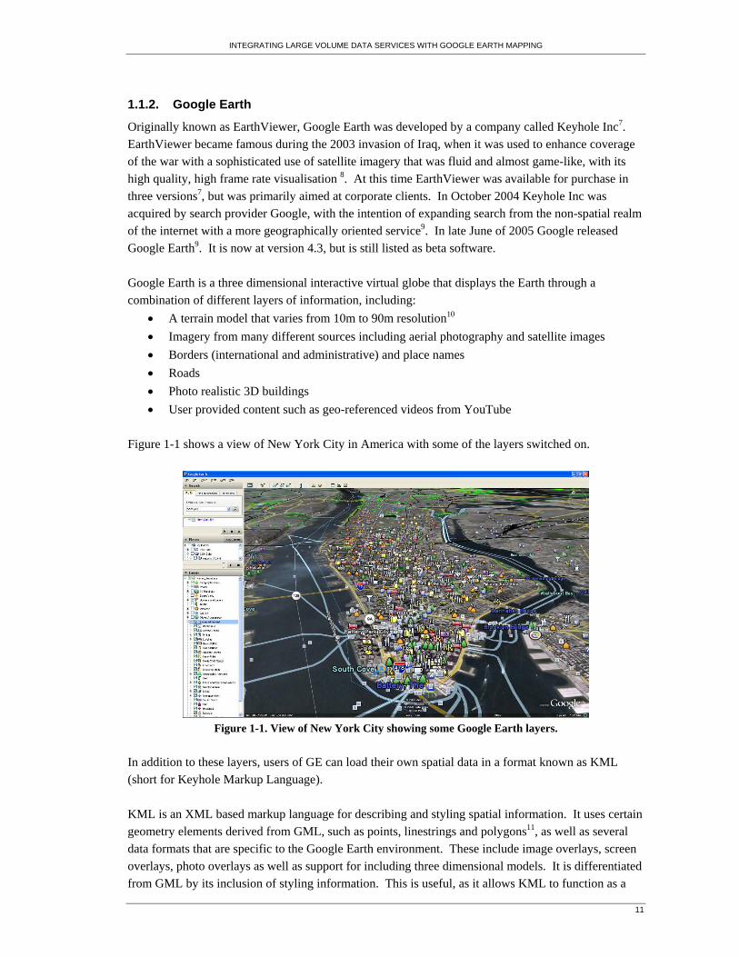
Figure 1-1 shows a view of New York City in America with some of the layers switched on.
Figure 1-1. View of New York City showing some Google Earth layers.
In addition to these layers, users of GE can load their own spatial data in a format known as KML
(short for Keyhole Markup Language).
KML is an XML based markup language for describing and styling spatial information. It uses certain
geometry elements derived from GML, such as points, linestrings and polygons11, as well as several
data formats that are specific to the Google Earth environment. These include image overlays, screen
overlays, photo overlays as well as support for including three dimensional models. It is differentiated
from GML by its inclusion of styling information. This is useful, as it allows KML to function as a
INTEGRATING LARGE VOLUME DATA SERVICES WITH GOOGLE EARTH MAPPING
12
form of vector WMS output. KML is currently at version 2.2, and has recently received OGC
specification status12. This is important, as any interoperable GDI should attempt to utilise as many
standards based methods and data formats as possible to try and maximise interoperability13. The full
KML schema can be found here: http://code.google.com/apis/kml/documentation/kmlreference.html.
One of the more advanced features of KML is the network link. This allows the connection of remote
sources of data, typically other KML files either on the local machine, or hosted elsewhere. The
benefit in this case is the ability to use Network Links to point to the output of a KML enabled WMS
or WFS. Provided the service outputs KML, this can be read by Google Earth, and if Google Earth is
set to refresh every time the view changes, then new data will be served, and a dynamic selection of
data from the server will occur. This will be used in this project to connect to the WMS.
1.1.3. Open Street Map Data
The Open Street Map (OSM) Project is a community created, freely available mapping dataset. The
features are created by contributors using GPS or survey devices, and are combined through wiki-style
collaborative software. Provided they have access to the internet, anybody is able to use the data
contained in the OSM, either by retrieving a pre-rendered image or by downloading the data14. There
are currently OSM mapping projects running all over the world on all the major continents in a total of
112 countries14.
The data that will be used in this project have been donated to the OSM Project by Automotive
Navigation Data16, with the intention to help contribute to the most up-to-date open mapping in the
world17. The dataset consists of transport, land use and other location data within the Netherlands.
1.2. Objectives
There are two main topics for this project:
1. Develop a method to serve the data to Google Earth as efficiently as possible.
2. Stylise the Open Street Map data in as cartographically correct a manner as possible in the
Google Earth environment, to ensure optimal interpretation by the user.
INTEGRATING LARGE VOLUME DATA SERVICES WITH GOOGLE EARTH MAPPING
13
2. Open Street Map Data
The Open Street Map data were originally provided in the form of shapefiles, which were loaded into
the PostgreSQL relational database management system using the shp2psql shapefile loader tool.
Each layer is stored in a different table, consisting of a unique identifier, several attributes and two
geometry columns. The geometry of the features is stored in both Dutch RD and WGS84 lat-long
projection systems. The number of attributes varies with each layer. Some of the attributes are
descriptive, while others are used as system attributes for the route planning software that uses these
data in GPS devices, and as such are not suitable for the purposes of this project.
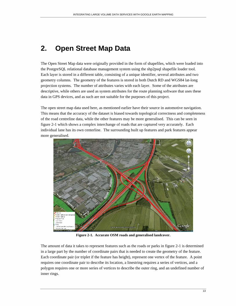
The open street map data used here, as mentioned earlier have their source in automotive navigation.
This means that the accuracy of the dataset is biased towards topological correctness and completeness
of the road centreline data, while the other features may be more generalised. This can be seen in
figure 2-1 which shows a complex interchange of roads that are captured very accurately. Each
individual lane has its own centerline. The surrounding built up features and park features appear
more generalised.
Figure 2-1. Accurate OSM roads and generalised landcover.
The amount of data it takes to represent features such as the roads or parks in figure 2-1 is determined
in a large part by the number of coordinate pairs that is needed to create the geometry of the feature.
Each coordinate pair (or triplet if the feature has height), represent one vertex of the feature. A point
requires one coordinate pair to describe its location, a linestring requires a series of vertices, and a
polygon requires one or more series of vertices to describe the outer ring, and an undefined number of
inner rings.
INTEGRATING LARGE VOLUME DATA SERVICES WITH GOOGLE EARTH MAPPING
14
The complexity of the data varies between layers. Generally the higher the number of vertices per
layer, the larger the scale at which it should be displayed, and the higher the likelihood that it should
be displayed as an image to get acceptable performance. Some layers have an extremely large number
of vertices, such as the road layer, while others are very simple, such as the Airport boundaries, or the
railway stations. This has an impact on the amount of data that is necessary to pass over the network
from the data sources to Google Earth, and can help determine the scale at which the data should be
displayed. It also has an impact on whether the data should be displayed as an image or as features.
There are two layers in particular that contain a large number of features, and are worth exploring - the
“Roads” and “Nodes” layers. The Roads layer contains 1,037,773 features comprising a geometric
representation of the road network of the Netherlands. In the specifications of the AND dataset, these
roads are classified twice, firstly by their type, and secondly by the scale at which they are displayed.
There are seven main road types in the dataset, and two supplementary types. They are represented by
integer values in the rd_5 attribute, and range from 1-7, plus 50 and 59 for the two extra types. Values
1-6 represent physical roads decreasing in size from motorways to other roads, while 7 is for ferries
that carry cars and cargo. The value 50 is for connections to railways and airports, while 59 is a
virtual connection that is used to connect features that are not otherwise connected by other features in
the database.
It would be impractical, both performance wise and cartographically to display all the road features at
once, so they have been split up into several layers. Each layer comes from the AND specifications,
and has a predefined scale at which it is suitable for display. These layers are defined by integer
values in the rd_7 attribute. They range in recommended scales from 1:4,000,000 to 1:250,000. Each
scale range is comprised of different types of roads that provide connections between locations of
varying significance. These locations can be found in the Nodes dataset. The nodes have a much
more limited number of features compared to the roads table, but as they are linked to the roads by the
recommended scales, it makes sense to divide them into layers with the same scale dependencies that
are found in the roads layers. While the nodes layer contains many different classes of features, for the
purposes of this work only the cities have been selected from the dataset. For more detailed
information about the roads and nodes layers please see Appendix 1.
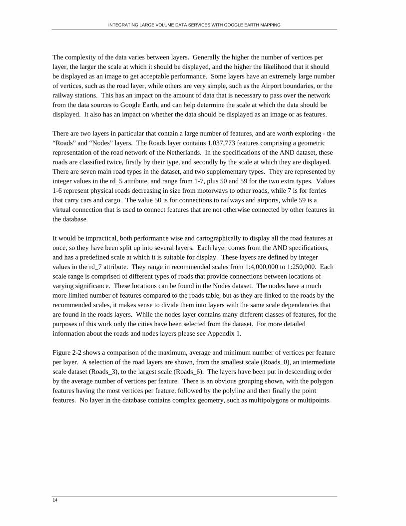
Figure 2-2 shows a comparison of the maximum, average and minimum number of vertices per feature
per layer. A selection of the road layers are shown, from the smallest scale (Roads_0), an intermediate
scale dataset (Roads_3), to the largest scale (Roads_6). The layers have been put in descending order
by the average number of vertices per feature. There is an obvious grouping shown, with the polygon
features having the most vertices per feature, followed by the polyline and then finally the point
features. No layer in the database contains complex geometry, such as multipolygons or multipoints.
INTEGRATING LARGE VOLUME DATA SERVICES WITH GOOGLE EARTH MAPPING
15
Figure 2-2. Comparison of vertices per feature, for several selected OSM layers.
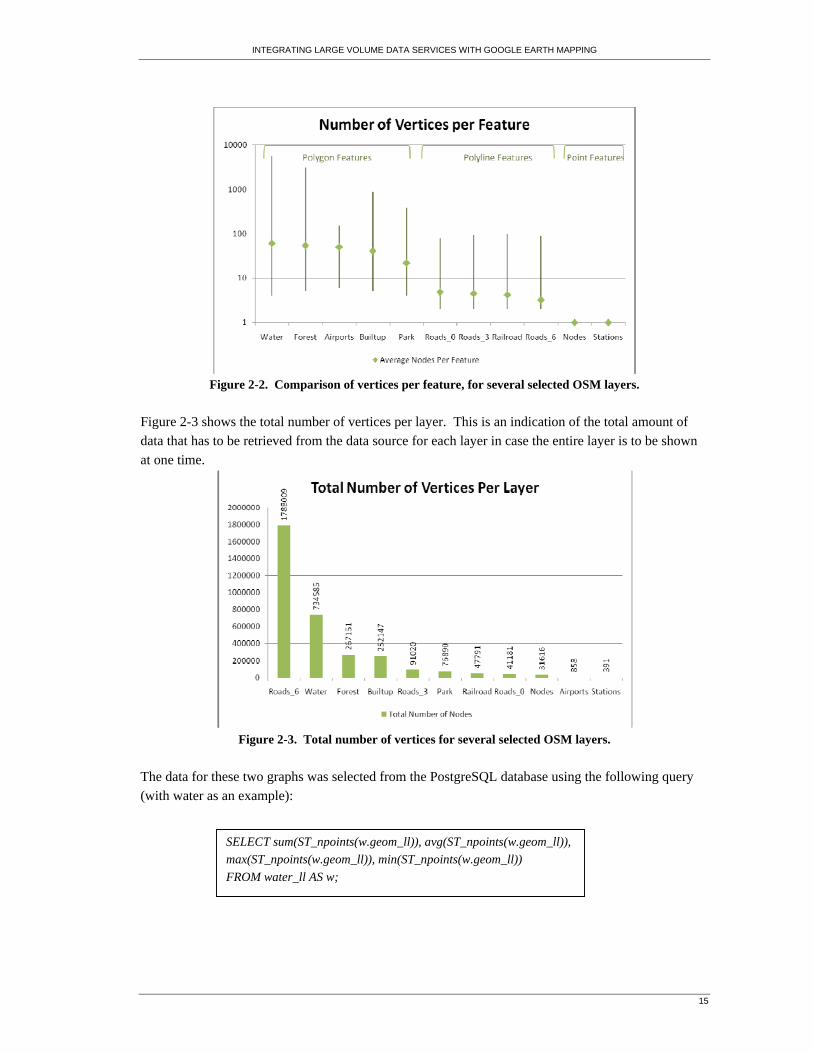
Figure 2-3 shows the total number of vertices per layer. This is an indication of the total amount of
data that has to be retrieved from the data source for each layer in case the entire layer is to be shown
at one time.
Figure 2-3. Total number of vertices for several selected OSM layers.
The data for these two graphs was selected from the PostgreSQL database using the following query
(with water as an example):
SELECT sum(ST_npoints(w.geom_ll)), avg(ST_npoints(w.geom_ll)),
max(ST_npoints(w.geom_ll)), min(ST_npoints(w.geom_ll))
FROM water_ll AS w;
INTEGRATING LARGE VOLUME DATA SERVICES WITH GOOGLE EARTH MAPPING
16
3. Options for KML Generation
A selection of different KML serving architectures were investigated, and in some cases limited testing
was undertaken in order to select the most promising option for further work.
3.1. ArcGIS Server
Currently at version 9.3, ArcGIS Server is high performance proprietary server software developed by
ESRI. ArcGIS Server offers KML output from datastores and geoprocessing tasks18. However as it is
commercial software, its cost could be outside the budget of many users. Taking this into account,
along with reasons from the FOSS4G conference presentation by Saul Farber
(http://www.foss4g2007.org/presentations/view.php?abstract_id=8) open source software was
preferred.
3.2. FME Server
FME Server is a spatial ETL (Extract, Transform, Load) software from Safe Software. It is able to
read many different data types, reproject, adjust attributes, merge and combine datasets, and finally
export data into many different formats including KML. Like ArcGIS Server, this is commercial
software, and so requires investment. Also, as it is powerful, but also quite complex, it requires investment in time as well as money.
3.3. KML MapServer
One of the most popular WMS currently is UMN MapServer. It is a widely used system for delivering
a variety of vector and raster data to users via the internet. It is primarily used for rendering images of
the data through client software such as OpenLayers running in a web browser. It is also able to serve
vector features via WFS. If this is combined with the KML MapServer project, then KML can be
served from the MapServer. However, KML MapServer does not currently support a bounding box,
meaning that all the data for each layer will be loaded every time the map is refreshed. For the
complex features that are going to be used in this project, this is not appropriate.
3.4. WFS-KML Gateway
WFS-KML Gateway is a promising project that is currently under development by Eduardo Riesco at
Universidad de Valladolid in Spain. It can be placed into any servlet container on a web server and
immediately start serving KML from a WFS. However, as it is still in development, there are many
bugs. For example, it currently only supports polygon rendering. Furthermore, there are issues
associated with the way it parses geometry from GML to KML that result in incorrect geometry in
Google Earth. As it reads WFS rather than WMS, this tool currently has no support for styling. With
further development it could have potential for statistical display of data, as it will have a strong
emphasis on the three dimensional display of features, which can be useful for emphasising trends.
INTEGRATING LARGE VOLUME DATA SERVICES WITH GOOGLE EARTH MAPPING
17
3.5. GeoServer KML
GeoServer is a fully featured WMS/WFS, with an easy set up process and a good interface. It reads
several popular data types, and can generate KML easily. As this is the option selected for the
completion of the project, further details are provided in the following sections of the report.
INTEGRATING LARGE VOLUME DATA SERVICES WITH GOOGLE EARTH MAPPING
18
4. Selected KML Generation Method
4.1. GeoServer
GeoServer was developed in 2001 by the Open Planning Project (OPP). The intention of GeoServer
was to help create a more open, interoperable infrastructure of geographic information. It was
specifically directed towards governmental offices that may be mandated to make their data available,
but lack the technical capacity to do so19. It is focused on the WFS side of geo-web services, with
emphasis on optimising the delivery of geographic features and attributes, rather than just images of
the data, however it is still a competent WMS.
Availability of GeoServer is via the geoserver.org website that hosts the GeoServer software, and
provides news, a forum, a “wiki-style” encyclopaedia, demonstration datasets and tutorials for using
various aspects of GeoServer.
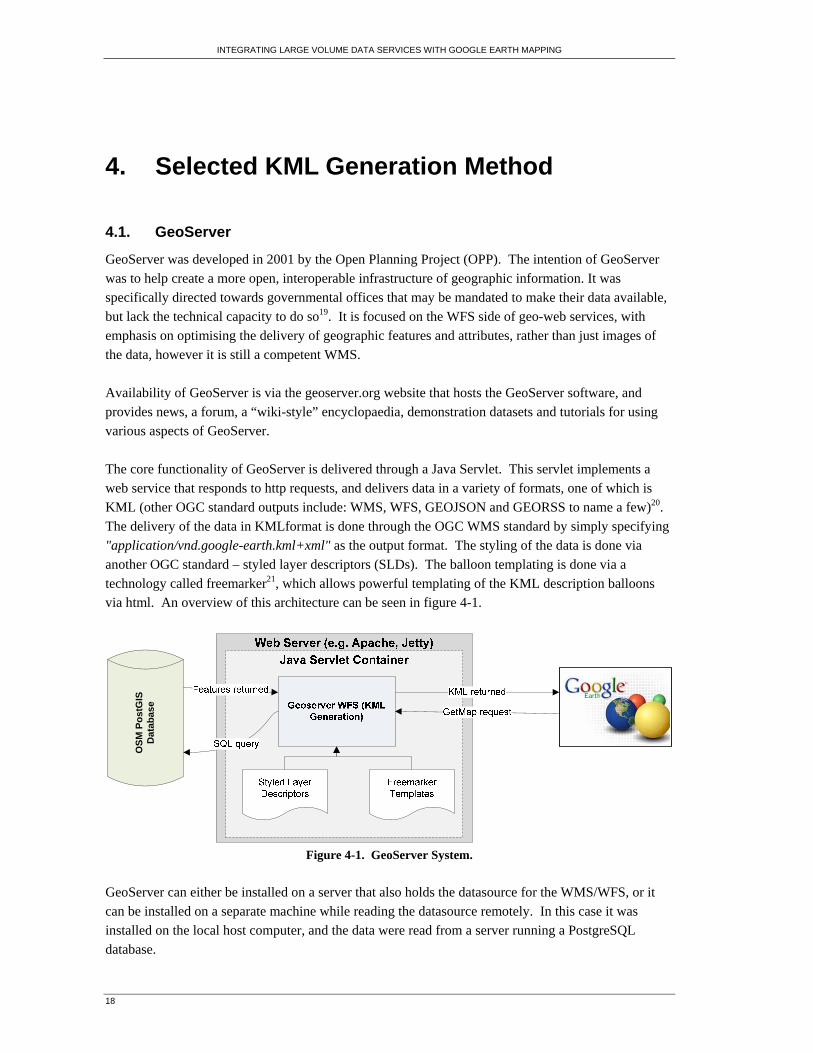
The core functionality of GeoServer is delivered through a Java Servlet. This servlet implements a
web service that responds to http requests, and delivers data in a variety of formats, one of which is
KML (other OGC standard outputs include: WMS, WFS, GEOJSON and GEORSS to name a few)20.
The delivery of the data in KMLformat is done through the OGC WMS standard by simply specifying
"application/vnd.google-earth.kml+xml" as the output format. The styling of the data is done via
another OGC standard – styled layer descriptors (SLDs). The balloon templating is done via a
technology called freemarker21, which allows powerful templating of the KML description balloons via html. An overview of this architecture can be seen in figure 4-1.
OS
M P
ost
GIS
D
ata
bas
e
Figure 4-1. GeoServer System.
GeoServer can either be installed on a server that also holds the datasource for the WMS/WFS, or it
can be installed on a separate machine while reading the datasource remotely. In this case it was
installed on the local host computer, and the data were read from a server running a PostgreSQL
database.
INTEGRATING LARGE VOLUME DATA SERVICES WITH GOOGLE EARTH MAPPING
19
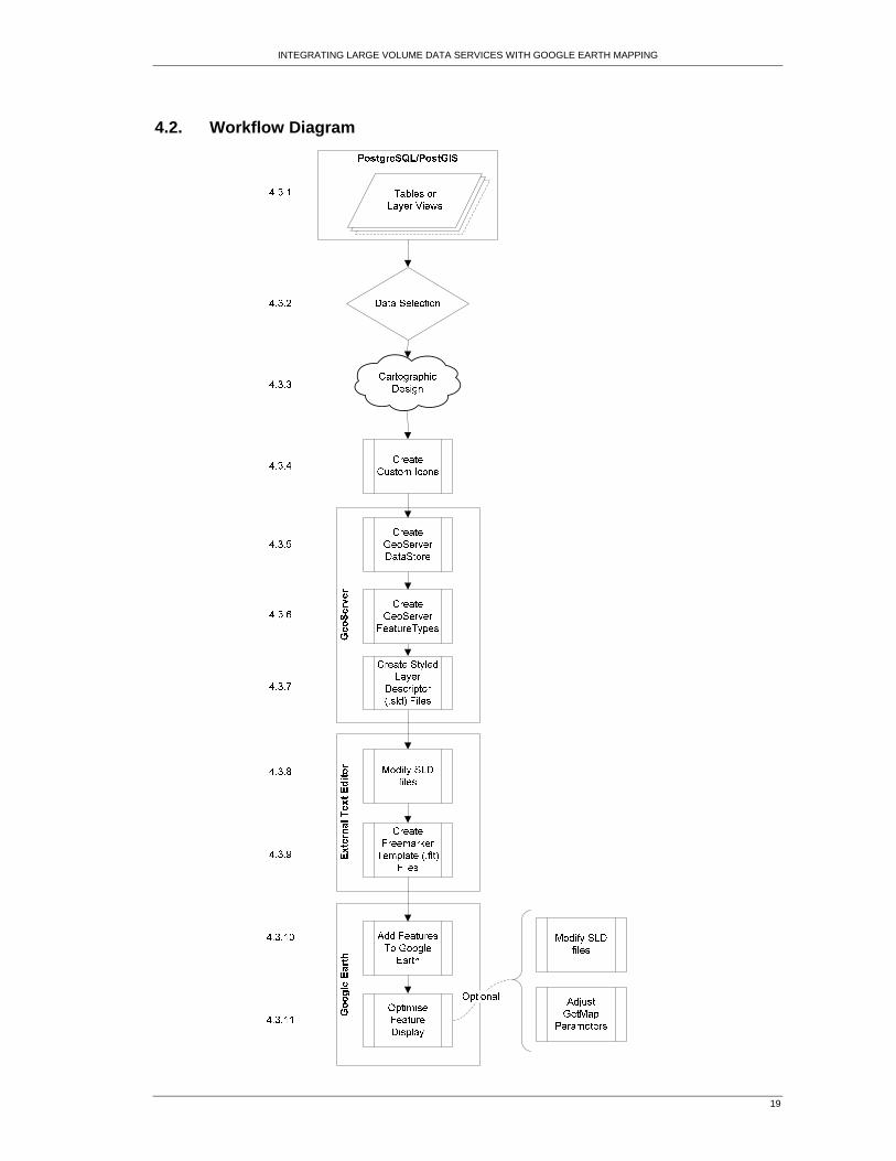
4.2. Workflow Diagram
INTEGRATING LARGE VOLUME DATA SERVICES WITH GOOGLE EARTH MAPPING
20
4.3. Description of the Workflow Steps
4.3.1. Data Preparation
The OSM data are stored in a relational PostgreSQL database hosted on the ITC server pubnt03.itc.nl.
It is important to ensure that the user who is working in GeoServer has access rights to the tables
and/or views that they will need from this database. The database is spatially extended using PostGIS,
which adds a selection of spatial operators and feature types to the database. Each spatially enabled
table in the database has two geometry columns, one for the Dutch RD coordinate system, and one for
WGS84 lat-long. GeoServer does not currently support multiple geometry columns, so it is necessary
to create views that only have one geometry column21. This is also useful, as it is appropriate to
examine the attributes of the data and select only the most relevant ones to display. If there are many
attributes that are intended for system use, such as unique identifiers, or columns to enable joins, then
these can be left out of the views. These do not need to be shown, and reducing the number of
attributes reduces the amount of data that needs to be generated and distributed. Also, it is possible to
add in information from non-spatial tables through a join into the view and expose this information to
GeoServer.
To improve performance attributes that may be queried by GeoServer for feature definitions can be
indexed. Spatial indices should be applied to the geometry columns to speed up the bounding box
intersection queries. All the views were created using the geometry columns that store the coordinates
in WGS84 (EPSG code: 4326), as this is the projection system supported by Google Earth23.
4.3.2. Data Selection
Depending on purpose of the user, some of the information included in the tables might not be
necessary. In this case not all the tables that are present in the database need to be served via
GeoServer to Google Earth. For example there is a table that displays a lat-long grid over the
Netherlands. This may be useful in a WMS that does not have a built in grid, but as Google Earth can
display WGS84 grid lines as an option, this dataset is redundant. Additionally there are other datasets
that may not be necessary to serve such as the country border. Google Earth has many of the internal
and external borders for the Netherlands, already cached and optimized for viewing. The selection of
the layers made available via Google Earth can be seen in table 4-1.
Table 4-1. Layers served from GeoServer.
Layer Name Levels Layer Group
Airports_ll 1
OSM_Landcover Builtup_ll 1
Forest_ll 1
Industrial_ll 1
Nodes_ll 7 OSM_Cities
Park_ll 1 OSM_Landcover
Railroad_ll 1 OSM_Transport
Roads_ll 7 OSM_Transport
Sea_ll 1 OSM_Landcover
Stations_ll 1 OSM_Transport
Water_ll 1 OSM_Landcover
INTEGRATING LARGE VOLUME DATA SERVICES WITH GOOGLE EARTH MAPPING
21
Once the required datasets have been chosen, the data can be further subset. When writing the queries
to create the views it is possible to select only records that meet certain prerequisites for some
attributes. For example, when creating the Nodes view the developer could select only the features
that represent cities of a certain size, or exit points from the motorways. Here, the decision was made
to keep all the features, so they could be adjusted at a later date, once there was increased familiarity
with the data. An alternative way of selecting which data will be displayed from the layers is
discussed in sections 4.3.7 and 4.3.8 on SLDs.
4.3.3. Cartographic Design
The different layers have varying requirements for symbolisation. Point, polyline or polygon features
each have to be symbolised in a different way. Additionally the layers may only be visible at certain
scales, so the symbology needs to be appropriate to be viewed at the scale that the layer is going to be
viewed. If the layers are going to have labels, then the attributes that are going to populate these labels
need to be selected. Additionally, the attributes that are going to be present in the description balloons
need to be chosen, so they can be incorporated later in the freemarker templates (more detail will be
discussed in section 4.3.9.)
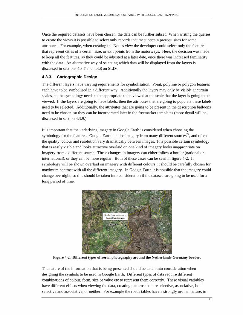
It is important that the underlying imagery in Google Earth is considered when choosing the
symbology for the features. Google Earth obtains imagery from many different sources24, and often
the quality, colour and resolution vary dramatically between images. It is possible certain symbology
that is easily visible and looks attractive overlaid on one kind of imagery looks inappropriate on
imagery from a different source. These changes in imagery can either follow a border (national or
international), or they can be more regular. Both of these cases can be seen in figure 4-2. If
symbology will be shown overlaid on imagery with different colours, it should be carefully chosen for
maximum contrast with all the different imagery. In Google Earth it is possible that the imagery could
change overnight, so this should be taken into consideration if the datasets are going to be used for a
long period of time.
Figure 4-2. Different types of aerial photography around the Netherlands-Germany border.
The nature of the information that is being presented should be taken into consideration when
designing the symbols to be used in Google Earth. Different types of data require different
combinations of colour, form, size or value etc to represent them correctly. These visual variables
have different effects when viewing the data, creating patterns that are selective, associative, both
selective and associative, or neither. For example the roads tables have a strongly ordinal nature, in
INTEGRATING LARGE VOLUME DATA SERVICES WITH GOOGLE EARTH MAPPING
22
that there are classes that can be viewed in a heirachy of importance, from the motorways to the local
roads. This is best represented by a combination of value and size, to create this ordered perception in
the viewers mind.
The data needs to be displayed in a way that could be considered “atlas-like”, so the features should be
displayed in a manner that is familiar to the users. There are certain conventions that can make
features more readily identifiable to users. In this case, there are two layers that represent water – the
sea and water layers. These will be shown in blue. There are also two layers that represent more
natural vegetation features, forests and parks, so these will be shown in two different shades of green.
The forests are shown in a darker green, and it appears denser than the lighter green of the parks. The
roads are shown with a symbology that is similar to many road maps and online mapping sites.
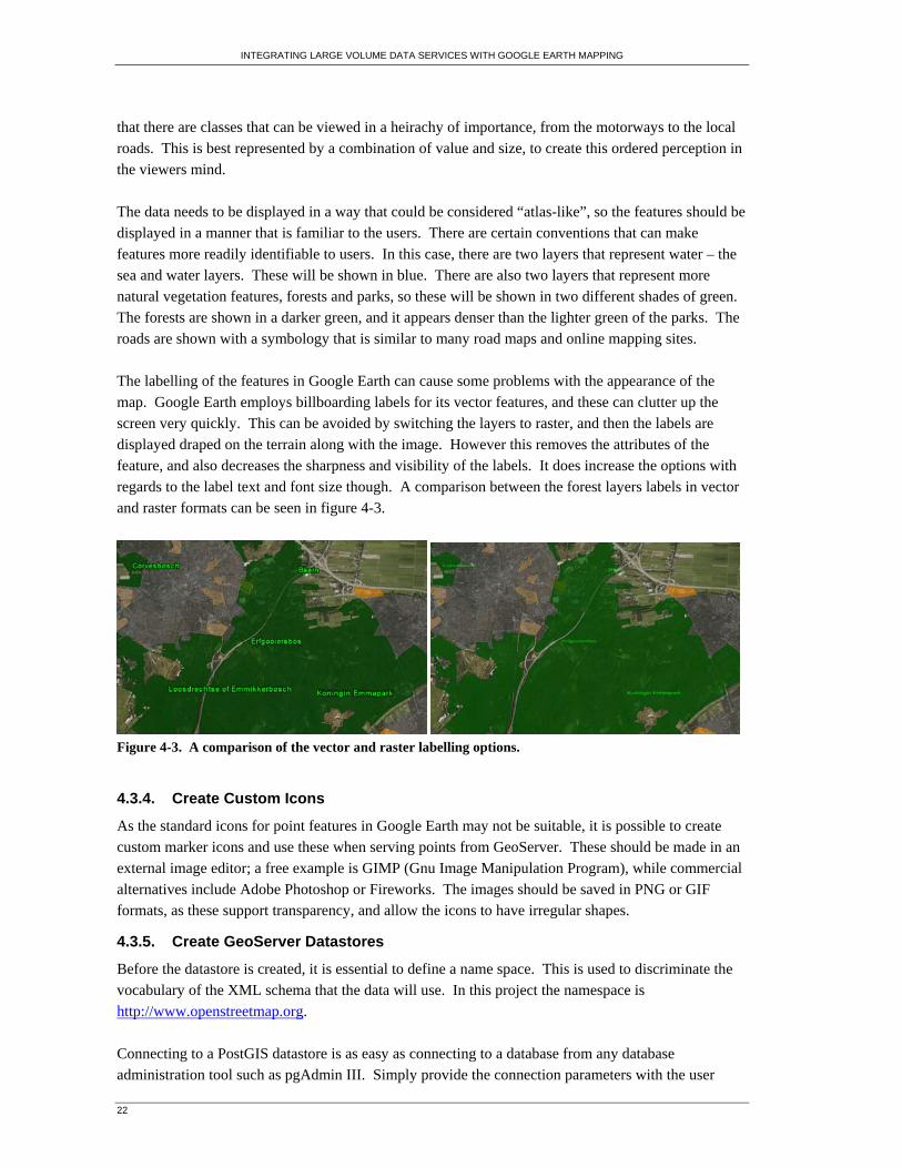
The labelling of the features in Google Earth can cause some problems with the appearance of the
map. Google Earth employs billboarding labels for its vector features, and these can clutter up the
screen very quickly. This can be avoided by switching the layers to raster, and then the labels are
displayed draped on the terrain along with the image. However this removes the attributes of the
feature, and also decreases the sharpness and visibility of the labels. It does increase the options with
regards to the label text and font size though. A comparison between the forest layers labels in vector
and raster formats can be seen in figure 4-3.
Figure 4-3. A comparison of the vector and raster labelling options.
4.3.4. Create Custom Icons
As the standard icons for point features in Google Earth may not be suitable, it is possible to create
custom marker icons and use these when serving points from GeoServer. These should be made in an
external image editor; a free example is GIMP (Gnu Image Manipulation Program), while commercial
alternatives include Adobe Photoshop or Fireworks. The images should be saved in PNG or GIF formats, as these support transparency, and allow the icons to have irregular shapes.
4.3.5. Create GeoServer Datastores
Before the datastore is created, it is essential to define a name space. This is used to discriminate the
vocabulary of the XML schema that the data will use. In this project the namespace is
http://www.openstreetmap.org.
Connecting to a PostGIS datastore is as easy as connecting to a database from any database
administration tool such as pgAdmin III. Simply provide the connection parameters with the user
INTEGRATING LARGE VOLUME DATA SERVICES WITH GOOGLE EARTH MAPPING
23
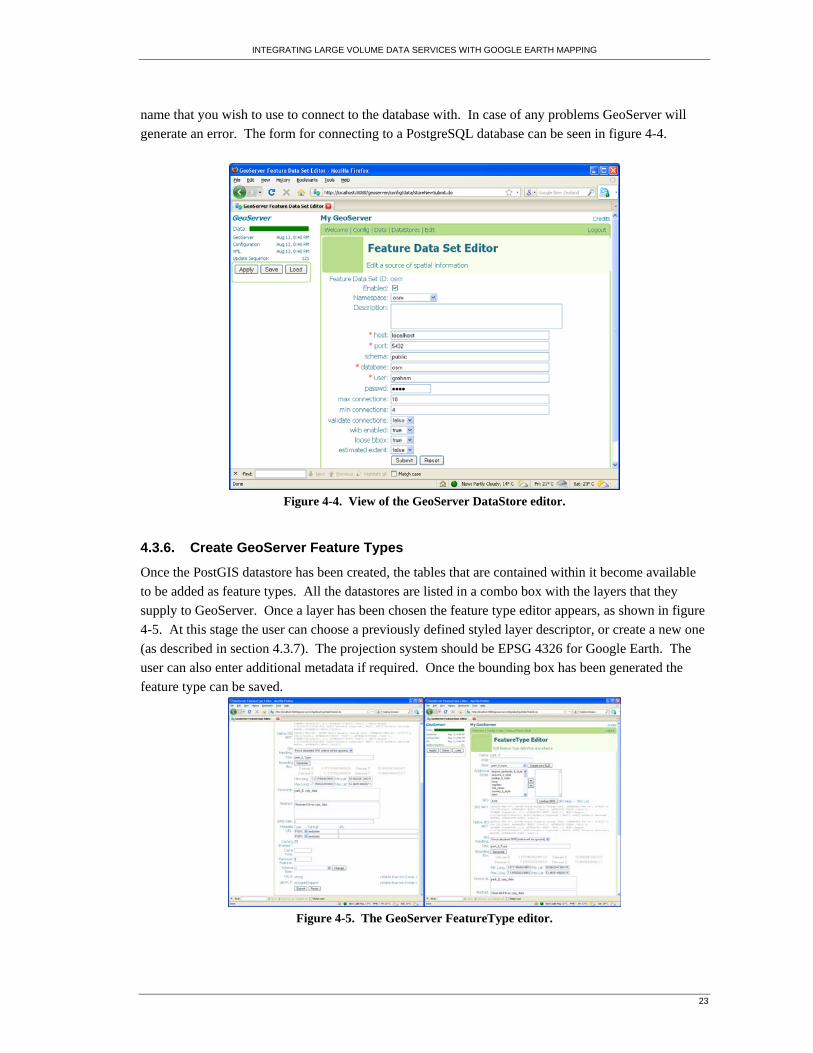
name that you wish to use to connect to the database with. In case of any problems GeoServer will
generate an error. The form for connecting to a PostgreSQL database can be seen in figure 4-4.
Figure 4-4. View of the GeoServer DataStore editor.
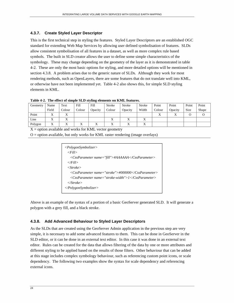
4.3.6. Create GeoServer Feature Types
Once the PostGIS datastore has been created, the tables that are contained within it become available
to be added as feature types. All the datastores are listed in a combo box with the layers that they
supply to GeoServer. Once a layer has been chosen the feature type editor appears, as shown in figure
4-5. At this stage the user can choose a previously defined styled layer descriptor, or create a new one
(as described in section 4.3.7). The projection system should be EPSG 4326 for Google Earth. The
user can also enter additional metadata if required. Once the bounding box has been generated the
feature type can be saved.
Figure 4-5. The GeoServer FeatureType editor.
INTEGRATING LARGE VOLUME DATA SERVICES WITH GOOGLE EARTH MAPPING
24
4.3.7. Create Styled Layer Descriptor
This is the first technical step in styling the features. Styled Layer Descriptors are an established OGC
standard for extending Web Map Services by allowing user defined symbolisation of features. SLDs
allow consistent symbolisation of all features in a dataset, as well as more complex rule based
symbols. The built in SLD creator allows the user to define some simple characteristics of the
symbology. These may change depending on the geometry of the layer as it is demonstrated in table
4-2. These are only the most basic options for styling, and more detailed options will be mentioned in
section 4.3.8. A problem arises due to the generic nature of SLDs. Although they work for most
rendering methods, such as OpenLayers, there are some features that do not translate well into KML,
or otherwise have not been implemented yet. Table 4-2 also shows this, for simple SLD styling
elements in KML.
Table 4-2. The effect of simple SLD styling elements on KML features. Geometry Name
Field
Text
Colour
Fill
Colour
Fill
Opacity
Stroke
Colour
Stroke
Opacity
Stroke
Width
Point
Colour
Point
Opacity
Point
Size
Point
Shape
Point X X X X O O
Line X X X X X
Polygon X X X X X X X
X = option available and works for KML vector geometry
O = option available, but only works for KML raster rendering (image overlays)
Above is an example of the syntax of a portion of a basic GeoServer generated SLD. It will generate a
polygon with a grey fill, and a black stroke.
4.3.8. Add Advanced Behaviour to Styled Layer Descriptors
As the SLDs that are created using the GeoServer Admin application in the previous step are very
simple, it is necessary to add some advanced features to them. This can be done in GeoServer in the
SLD editor, or it can be done in an external text editor. In this case it was done in an external text
editor. Rules can be created for the data that allows filtering of the data by one or more attributes and
different styling to be applied based on the results of those filters. Other behaviour that can be added at this stage includes complex symbology behaviour, such as referencing custom point icons, or scale
dependency. The following two examples show the syntax for scale dependency and referencing
external icons.
<PolygonSymbolizer>
<Fill>
<CssParameter name="fill">#AAAAAA</CssParameter>
</Fill>
<Stroke>
<CssParameter name="stroke">#000000</CssParameter>
<CssParameter name="stroke-width">1</CssParameter>
</Stroke>
</PolygonSymbolizer>
INTEGRATING LARGE VOLUME DATA SERVICES WITH GOOGLE EARTH MAPPING
25
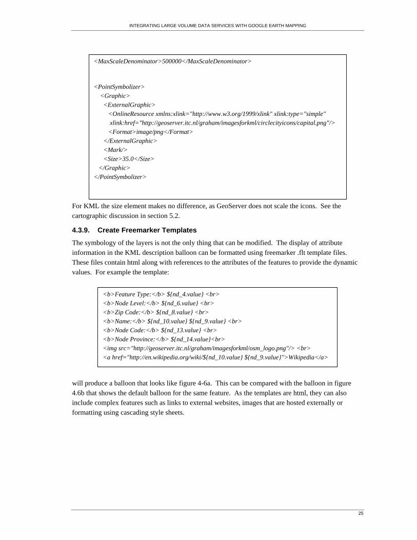
For KML the size element makes no difference, as GeoServer does not scale the icons. See the
cartographic discussion in section 5.2.
4.3.9. Create Freemarker Templates
The symbology of the layers is not the only thing that can be modified. The display of attribute
information in the KML description balloon can be formatted using freemarker .flt template files.
These files contain html along with references to the attributes of the features to provide the dynamic
values. For example the template:
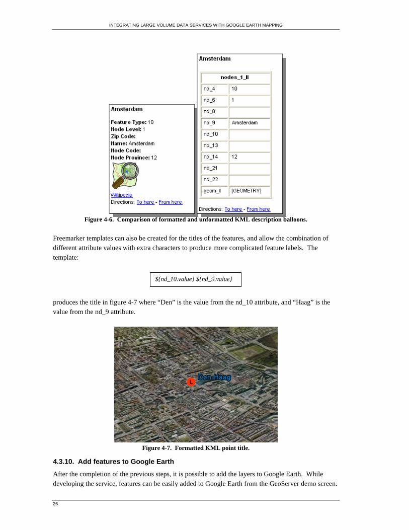
will produce a balloon that looks like figure 4-6a. This can be compared with the balloon in figure
4.6b that shows the default balloon for the same feature. As the templates are html, they can also include complex features such as links to external websites, images that are hosted externally or
formatting using cascading style sheets.
<b>Feature Type:</b> ${nd_4.value} <br>
<b>Node Level:</b> ${nd_6.value} <br>
<b>Zip Code:</b> ${nd_8.value} <br>
<b>Name:</b> ${nd_10.value} ${nd_9.value} <br>
<b>Node Code:</b> ${nd_13.value} <br>
<b>Node Province:</b> ${nd_14.value}<br>
<img src="http://geoserver.itc.nl/graham/imagesforkml/osm_logo.png"/> <br>
<a href="http://en.wikipedia.org/wiki/${nd_10.value} ${nd_9.value}">Wikipedia</a>
<MaxScaleDenominator>500000</MaxScaleDenominator>
<PointSymbolizer>
<Graphic>
<ExternalGraphic>
<OnlineResource xmlns:xlink="http://www.w3.org/1999/xlink" xlink:type="simple"
xlink:href="http://geoserver.itc.nl/graham/imagesforkml/circlecityicons/capital.png"/>
<Format>image/png</Format>
</ExternalGraphic>
<Mark/>
<Size>35.0</Size>
</Graphic>
</PointSymbolizer>
INTEGRATING LARGE VOLUME DATA SERVICES WITH GOOGLE EARTH MAPPING
26
Figure 4-6. Comparison of formatted and unformatted KML description balloons.
Freemarker templates can also be created for the titles of the features, and allow the combination of
different attribute values with extra characters to produce more complicated feature labels. The
template:
produces the title in figure 4-7 where “Den” is the value from the nd_10 attribute, and “Haag” is the
value from the nd_9 attribute.
Figure 4-7. Formatted KML point title.
4.3.10. Add features to Google Earth
After the completion of the previous steps, it is possible to add the layers to Google Earth. While
developing the service, features can be easily added to Google Earth from the GeoServer demo screen.
${nd_10.value} ${nd_9.value}
INTEGRATING LARGE VOLUME DATA SERVICES WITH GOOGLE EARTH MAPPING
27
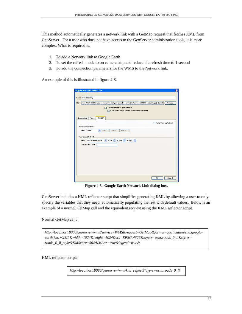
This method automatically generates a network link with a GetMap request that fetches KML from
GeoServer. For a user who does not have access to the GeoServer administration tools, it is more
complex. What is required is:
1. To add a Network link to Google Earth
2. To set the refresh mode to on camera stop and reduce the refresh time to 1 second
3. To add the connection parameters for the WMS to the Network link.
An example of this is illustrated in figure 4-8.
Figure 4-8. Google Earth Network Link dialog box.
GeoServer includes a KML reflector script that simplifies generating KML by allowing a user to only
specify the variables that they need, automatically populating the rest with default values. Below is an
example of a normal GetMap call and the equivalent request using the KML reflector script.
Normal GetMap call:
KML reflector script:
http://localhost:8080/geoserver/wms?service=WMS&request=GetMap&format=application/vnd.google-
earth.kmz+XML&width=1024&height=1024&srs=EPSG:4326&layers=osm:roads_0_ll&styles=
roads_0_ll_style&KMScore=50&KMAttr=true&legend=true&
http://localhost:8080/geoserver/wms/kml_reflect?layers=osm:roads_0_ll
INTEGRATING LARGE VOLUME DATA SERVICES WITH GOOGLE EARTH MAPPING
28
4.3.11. Optimise Feature Display
Once the layers have been added to Google Earth, it is possible to change the way they are displayed
by modifying some of the parameters that are included in the GetMap call. Specifically, one
parameter that makes a large difference to the performance and the cartographic output is the
KMScore. The KMScore is a value that determines the point at which the display of the layers in
Google Earth changes from vector to raster. When the number of features returned from the server
passes the threshold set in the KMScore, the layer is shown as an image rather than as vectors. The
KMScore is a log function, where 0 = always raster, and 100 = always vector. A plot of this function
can be seen in figure 4-9.
Figure 4-9. KMScore vs number of features displayed.
A choice can also be made between providing the attributes of the features or not using the KMAttr
option. If it is turned on then the features are available via an information point, while if it is turned
off then the point is not there and the attributes are not available. This also reduces the amount of
KML that has to be displayed, as the features do not include the extra geometry and attributes of the
information points.
GeoServer is able to generate a legend screenoverlay in Google Earth to assist the interpretation of the
features that are displayed in Google Earth. This can be seen in figure 4-10. It is the result of
changing another GetMap parameter – legend. If legend = true, the legend will be created. One
problem is the legends are not aware of conflicts, and they will overlap if more than one are created.
Figure 4-10. Roads layers showing legend generated in the Roads_0 layer.

INTEGRATING LARGE VOLUME DATA SERVICES WITH GOOGLE EARTH MAPPING
29
5. Results/Discussion
5.1. Performance
5.1.1. Implementation
Delivering KML from GeoServer is an easy process that should be relatively straight forward to
implement by anybody who has administered a web map service. It only requires some administration
in the current GeoServer service, and does not need any extra software to be installed, which simplifies
the procedure. It features a good graphical user interface, compared to alternatives like MapServer
that work primarily through editing the configuration mapfile. There is some manual text editing work
required to enable some of the more advanced features, but the comprehensive wiki and tutorials ease
the way for beginners.
GeoServer is very flexible taking into account all the different ways it can be set up. There are options
for optimisation along the whole data flow, from the type of data source used to the layers that are
selected to the display in Google Earth. These will be discussed as they occur in the following
sections.
The administration interface is not difficult to navigate, but still has some idiosyncrasies. Therefore
with the release of GeoServer 2.0 the interface will be getting a new design. GeoServer 2.0 is
currently in the very early alpha stage of development, but can be downloaded and installed if desired.
Figure 5-1 shows a comparison between the current and future interfaces.
Figure 5-1. Comparison of GeoServer 1.6.4 and 2.0 interfaces
INTEGRATING LARGE VOLUME DATA SERVICES WITH GOOGLE EARTH MAPPING
30
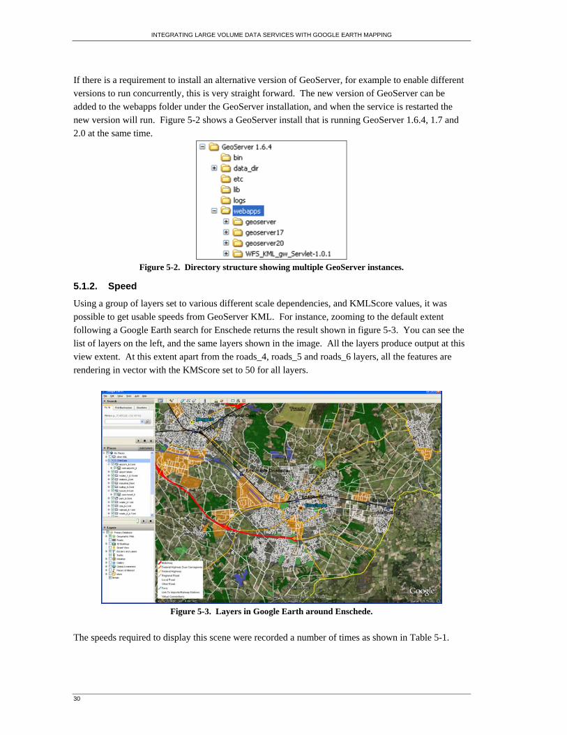
If there is a requirement to install an alternative version of GeoServer, for example to enable different
versions to run concurrently, this is very straight forward. The new version of GeoServer can be
added to the webapps folder under the GeoServer installation, and when the service is restarted the
new version will run. Figure 5-2 shows a GeoServer install that is running GeoServer 1.6.4, 1.7 and
2.0 at the same time.
Figure 5-2. Directory structure showing multiple GeoServer instances.
5.1.2. Speed
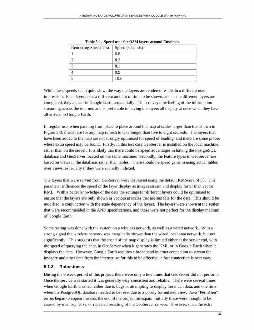
Using a group of layers set to various different scale dependencies, and KMLScore values, it was
possible to get usable speeds from GeoServer KML. For instance, zooming to the default extent
following a Google Earth search for Enschede returns the result shown in figure 5-3. You can see the
list of layers on the left, and the same layers shown in the image. All the layers produce output at this
view extent. At this extent apart from the roads_4, roads_5 and roads_6 layers, all the features are
rendering in vector with the KMScore set to 50 for all layers.
Figure 5-3. Layers in Google Earth around Enschede.
The speeds required to display this scene were recorded a number of times as shown in Table 5-1.
INTEGRATING LARGE VOLUME DATA SERVICES WITH GOOGLE EARTH MAPPING
31
Table 5-1. Speed tests for OSM layers around Enschede.
Rendering Speed Test Speed (seconds)
1 6.8
2 8.3
3 8.1
4 8.9
5 10.6
While these speeds seem quite slow, the way the layers are rendered results in a different user
impression. Each layer takes a different amount of time to be shown, and as the different layers are
completed, they appear in Google Earth sequentially. This conveys the feeling of the information streaming across the internet, and is preferable to having the layers all display at once when they have
all arrived to Google Earth.
In regular use, when panning from place to place around the map at scales larger than that shown in
Figure 5-3, it was rare for any map refresh to take longer than five to eight seconds. The layers that
have been added to the map are not strongly optimised for speed of loading, and there are some places
where extra speed may be found. Firstly, in this test case GeoServer is installed on the local machine,
rather than on the server. It is likely that there could be speed advantages in having the PostgreSQL
database and GeoServer located on the same machine. Secondly, the feature types in GeoServer are
based on views in the database, rather than tables. There should be speed gains in using actual tables
over views, especially if they were spatially indexed.
The layers that were served from GeoServer were displayed using the default KMScore of 50. This
parameter influences the speed of the layer display as images stream and display faster than vector
KML. With a better knowledge of the data the settings for different layers could be optimised to
ensure that the layers are only shown as vectors at scales that are suitable for the data. This should be
modified in conjunction with the scale dependency of the layers. The layers were shown at the scales
that were recommended in the AND specifications, and these were not perfect for the display medium
of Google Earth.
Some testing was done with the system on a wireless network, as well as a wired network. With a
strong signal the wireless network was marginally slower than the wired local area network, but not
significantly. This suggests that the speed of the map display is limited either at the server end, with
the speed of querying the data, in GeoServer when it generates the KML or in Google Earth when it
displays the data. However, Google Earth requires a broadband internet connection to stream the
imagery and other data from the internet, so for this to be effective, a fast connection is necessary.
5.1.3. Robustness
During the 6 week period of this project, there were only a few times that GeoServer did not perform.
Once the service was started it was generally very consistent and reliable. There were several times
when Google Earth crashed, either due to bugs or attempting to display too much data, and one time
when the PostgreSQL database needed to be reset due to a poorly formulated view. Java “PermGen”
errors began to appear towards the end of the project timespan. Initially these were thought to be
caused by memory leaks, or repeated resetting of the GeoServer service. However, once the extra
INTEGRATING LARGE VOLUME DATA SERVICES WITH GOOGLE EARTH MAPPING
32
GeoServer versions (1.7 RC2, 2.0 alpha) were removed from the webapps folder, leaving only 1.6.4
the service resumed operating correctly. This is possibly caused by the stripped down version of Jetty
6.2 that is shipped with GeoServer, and could be resolved by deploying GeoServer into a full install of
Apache or similar. An optimised server running a server specific operating system is more likely to
handle problems that can cause this kind of error.
5.1.4. Scalability
It is easy to make changes to the layers that are served through GeoServer, or to add new ones through
the administration interface. Style changes are simply a matter of editing textfiles, and there does not
appear to be a limit to the number of feature types that can be served, or to the maximum number of
features that can be served from each feature type. It is likely that the database, the network or Google
Earth will have trouble before GeoServer does. The database, the network and GeoServer all support
standard scaling measures, such as on-server caching, round robin load distribution or multi-tier server
architectures. Methods such as these can help to increase the performance of GeoServer as the number
of requests and amount of data increases.
5.1.5. Using Caching or Regionation
Two more advanced features that have not been implemented in this project are caching, and regionation. Caching refers to the act of rendering image tiles at different scales, then storing them on
the server for quick access at a later date. This technique is usually associated with WMS serving
images and can provide large performance gains, as the images do not have to be rendered so can be
retrieved and displayed very fast. This is not appropriate for this project, as raster representation of the
features is only required when there are too many features to allow the preferred vector display.
GeoServer claims to support vector caching with the optional GeoWebCache plugin, but it was not
possible to implement it during the time available.
Another method that has potential to improve performance is regionation. This is the process of
creating a hierarchy of NetworkLinks that each display a small amount of KML at a different scale.
The different layers that were used for this project have defined scales at which we want either all the
features to be present, or none of them. Therefore it was decided that regionation was not suitable for
these data. Regionation seems to be more suitable for large, unstructured data that would otherwise be
obscuring each other. A good example of this is the sample Swiss Transit dataset on the Google Code
webpage25.
5.2. Cartography
5.2.1. Styling
The OSM data used in this context is intended to serve as an analogue for the proposed National Atlas
dataset. Because of this it is important to consider the appropriateness of Google Earth as a way to
display this sort of data.
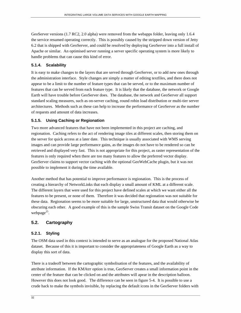
There is a tradeoff between the cartographic symbolisation of the features, and the availability of
attribute information. If the KMAtrr option is true, GeoServer creates a small information point in the
center of the feature that can be clicked on and the attributes will apear in the description balloon.
However this does not look good. The difference can be seen in figure 5-4. It is possible to use a
crude hack to make the symbols invisible, by replacing the default icons in the GeoServer folders with
INTEGRATING LARGE VOLUME DATA SERVICES WITH GOOGLE EARTH MAPPING
33
blank ones. This mean that the attributes can still be accessed, but it is difficult to find the right place
on a polyline to click on to get them. A polygon is easier, as a user can ctrl-click on any part of the
polygon to retrieve the attributes for that feature. The KML generated is still a multi-geometry, as it
has the polyline or polygon geometry, and a point geometry for the information point.
Figure 5-4. Attribute information points.
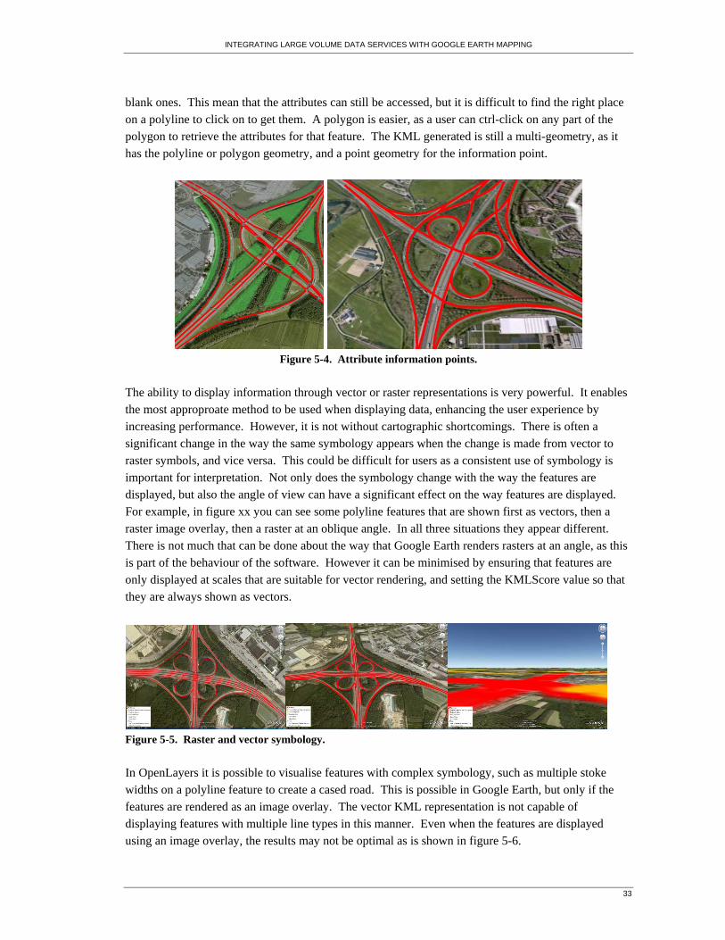
The ability to display information through vector or raster representations is very powerful. It enables
the most approproate method to be used when displaying data, enhancing the user experience by
increasing performance. However, it is not without cartographic shortcomings. There is often a
significant change in the way the same symbology appears when the change is made from vector to
raster symbols, and vice versa. This could be difficult for users as a consistent use of symbology is
important for interpretation. Not only does the symbology change with the way the features are
displayed, but also the angle of view can have a significant effect on the way features are displayed.
For example, in figure xx you can see some polyline features that are shown first as vectors, then a
raster image overlay, then a raster at an oblique angle. In all three situations they appear different.
There is not much that can be done about the way that Google Earth renders rasters at an angle, as this
is part of the behaviour of the software. However it can be minimised by ensuring that features are
only displayed at scales that are suitable for vector rendering, and setting the KMLScore value so that
they are always shown as vectors.
Figure 5-5. Raster and vector symbology.
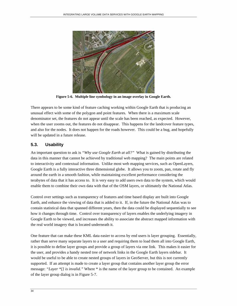
In OpenLayers it is possible to visualise features with complex symbology, such as multiple stoke
widths on a polyline feature to create a cased road. This is possible in Google Earth, but only if the
features are rendered as an image overlay. The vector KML representation is not capable of
displaying features with multiple line types in this manner. Even when the features are displayed
using an image overlay, the results may not be optimal as is shown in figure 5-6.
INTEGRATING LARGE VOLUME DATA SERVICES WITH GOOGLE EARTH MAPPING
34
Figure 5-6. Multiple line symbology in an image overlay in Google Earth.
There appears to be some kind of feature caching working within Google Earth that is producing an
unusual effect with some of the polygon and point features. When there is a maximum scale
denominator set, the features do not appear until the scale has been reached, as expected. However,
when the user zooms out, the features do not disappear. This happens for the landcover feature types,
and also for the nodes. It does not happen for the roads however. This could be a bug, and hopefully
will be updated in a future release.
5.3. Usability
An important question to ask is “Why use Google Earth at all?” What is gained by distributing the
data in this manner that cannot be achieved by traditional web mapping? The main points are related
to interactivity and contextual information. Unlike most web mapping services, such as OpenLayers,
Google Earth is a fully interactive three dimensional globe. It allows you to zoom, pan, rotate and fly around the earth in a smooth fashion, while maintaining excellent performance considering the
terabytes of data that it has access to. It is very easy to add users own data to the system, which would
enable them to combine their own data with that of the OSM layers, or ultimately the National Atlas.
Control over settings such as transparency of features and time based display are built into Google
Earth, and enhance the viewing of data that is added to it. If, in the future the National Atlas was to
contain statistical data that spanned different years, then the data could be displayed sequentially to see
how it changes through time. Control over transparency of layers enables the underlying imagery in
Google Earth to be viewed, and increases the ability to associate the abstract mapped information with
the real world imagery that is located underneath it.
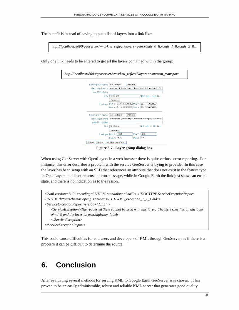
One feature that can make these KML data easier to access by end users is layer grouping. Essentially,
rather than serve many separate layers to a user and requiring them to load them all into Google Earth,
it is possible to define layer groups and provide a group of layers via one link. This makes it easier for
the user, and provides a handy nested tree of network links in the Google Earth layers sidebar. It
would be useful to be able to create nested groups of layers in GeoServer, but this is not currently
supported. If an attempt is made to create a layer group that contains another layer group the error
message: “Layer *[] is invalid.” Where * is the name of the layer group to be contained. An example
of the layer group dialog is in Figure 5-7.
INTEGRATING LARGE VOLUME DATA SERVICES WITH GOOGLE EARTH MAPPING
35
The benefit is instead of having to put a list of layers into a link like:
Only one link needs to be entered to get all the layers contained within the group:
Figure 5-7. Layer group dialog box.
When using GeoServer with OpenLayers in a web browser there is quite verbose error reporting. For
instance, this error describes a problem with the service GeoServer is trying to provide. In this case
the layer has been setup with an SLD that references an attribute that does not exist in the feature type.
In OpenLayers the client returns an error message, while in Google Earth the link just shows an error
state, and there is no indication as to the reason.
This could cause difficulties for end users and developers of KML through GeoServer, as if there is a
problem it can be difficult to determine the source.
6. Conclusion
After evaluating several methods for serving KML to Google Earth GeoServer was chosen. It has
proven to be an easily administrable, robust and reliable KML server that generates good quality
http://localhost:8080/geoserver/wms/kml_reflect?layers=osm:roads_0_ll,roads_1_ll,roads_2_ll...
http://localhost:8080/geoserver/wms/kml_reflect?layers=osm:osm_transport
<?xml version="1.0" encoding="UTF-8" standalone="no"?><!DOCTYPE ServiceExceptionReport
SYSTEM "http://schemas.opengis.net/wms/1.1.1/WMS_exception_1_1_1.dtd">
<ServiceExceptionReport version="1.1.1" >
<ServiceException>The requested Style cannot be used with this layer. The style specifies an attribute
of nd_9 and the layer is: osm:highway_labels
</ServiceException>
</ServiceExceptionReport>
INTEGRATING LARGE VOLUME DATA SERVICES WITH GOOGLE EARTH MAPPING
36
output. Speed testing showed that the performance results were acceptable, even with little
performance optimisation on the data, or on the server hardware and software. With an optimised
server setup and more attention to the configuration settings for the files very good performance will
be possible.
The OSM data served as a good approximation for potential National Atlas data. The data were not
optimised for display in Google Earth, which is likely to happen with the different potential National
Atlas datasets.
Cartographically GeoServer creates a good quality output. The Google Earth environment is not as
cartographically effective as a dedicated mapping service such as OpenLayers, and this is reflected in
the results. OpenLayers provides much finer control over symbology and labelling. There can be
problems with the way features appear when they change from vector to raster in Google Earth, but
this can be controlled through careful style configuration.
Creating KML through GeoServer is a very flexible method of getting diverse datasets into Google
Earth. It works well, even with datasets that are not well suited to this kind of mapping. It would be a
suitable option to serve KML for a National Atlas of Holland.
Google Earth allows a more immersive, interactive experience with the layers than a normal web map.
The ability to smoothly rotate, pan and zoom around the data, while it is overlayed on high quality
imagery enhances the user experience. The ability for users of the system to easily add their own data
increases the value of the service. The transparency of the OSM layers can be adjusted from within
Google Earth to enable the underlying imagery to be compared to the features that are being displayed.
Recommendations for improving the results are:
Optimising the datasets if possible by simplifying features and removing unnecessary amounts of detail. Ensure that all data is indexed, spatially and non-spatially.
Examining the datasets carefully and determining the best levels at which they should be
shown.
Using good cartographic methods to determine the correct symbology for the different layers,
taking into account the unique Google Earth environment.
Ensuring that the latest version of GeoServer is used. As it is constantly under development,
the latest versions always have new and improved features.
Optimising the server-side performance of the system by utilising the correct placement of
GeoServer on the server, rather than locally. Create a proper production setup, with dedicated
client-server architecture, allowing each machine to do its own job.
INTEGRATING LARGE VOLUME DATA SERVICES WITH GOOGLE EARTH MAPPING
37
References
1. Web Mapping (updated: 17/06/2008) http://en.wikipedia.org/wiki/Web_mapping (accessed:
19/06/2008)
2. Nebert, D. (2004) The SDI Cookbook Version 2.0
http://www.gsdi.org/docs2004/Cookbook/cookbookV2.0.pdf
3. Kraak, M. J. Et al (2007) The Dutch National Atlas in a GII Environment: The Application of
Design Templates; 23rd International Cartographic Conference
4. Beaujardiere, J. (2004) OGC Web Map Service Interface, OGC 03-109r1
http://portal.opengeospatial.org/files/?artifact_id=4756
5. Vretanos, P. A. (2005) Web Feature Service Implementation Specification, OGC 04-094
http://portal.opengeospatial.org/files/?artifact_id=8339
6. Portele, C. (2007) OpenGIS Georaphy Markup Language (GML) Encoding Standard, OGC
07-036 http://portal.opengeospatial.org/files/?artifact_id=20509
7. Keyhole Homepage (19/09/2003)
http://web.archive.org/web/20030919004249/http://www.keyhole.com/ (accessed:
06/07/2008)
8. Maney, K. Tiny tech company awes viewers (updated: 21/03/2003)
http://www.usatoday.com/tech/news/techinnovations/2003-03-20-earthviewer_x.htm
(accessed: 06/07/2008)
9. Google Corporate Information (updated: 21/07/2008)
http://www.google.com/corporate/history.html (accessed: 05/08/2008)
10. Google Earth update makes Alps sparkle (02/03/2007)
http://www.ogleearth.com/2007/03/google_earth_up_2.html (accessed: 17/06/2008)
11. OGC KML Standard (updated: 19/08/2008) http://www.opengeospatial.org/standards/kml/
(accessed: 04/08/2008)
12. OGC approves KML as a standard (updated: 13/04/2008)
http://www.opengeospatial.org/pressroom/pressreleases/857 (accessed: 15/07/2008)
13. Köbben, (2008) B. A Short Introduction to Geo-Web Services
14. Open Street Map: About (updated: 03/08/2008) http://wiki.openstreetmap.org/index.php/OpenStreetMap:About (accessed: 04/08/2008)
15. Open Street Map: Mapping Projects (updated: 13/08/2008)
http://wiki.openstreetmap.org/index.php/Mapping_projects (accessed: 13/08/2008)
16. Open Street Map: AND Data (updated: 12/07/2008)
http://wiki.openstreetmap.org/index.php/AND_Data (accessed: 02/08/2008)
INTEGRATING LARGE VOLUME DATA SERVICES WITH GOOGLE EARTH MAPPING
38
17. AND Newsletter http://www.and.com/company/newsletter/newsletter10/art01en.php
(accessed: 14/07/2008)
18. What’s New in ArcGIS http://www.esri.com/software/arcgis/about/whats-new.html (accessed:
15/08/2007)
19. The Open Planning Project: Motivations (updated: 12/01/2007)
http://www.openplans.org/projects/topp-the-organization/motivations (accessed: 10/08/2008)
20. GeoServer for Google Earth (updated: 06/08/2007)
http://geoserver.org/display/GEOSDOC/00+GeoServer+for+Google+Earth
(accessed:11/08/2008 )
21. Freemarker Templates (updated: 03/08/2007)
http://geoserver.org/display/GEOSDOC/Freemarker+templates (accessed: 01/08/2007)
22. My Geo follies (updated: 25/03/2008)
http://geoserver.org/display/GEOSDOC/My+Geo+follies?focusedCommentId=1279189#MyG
eofollies-Butthefilteredlayersareslow (accessed: 15/08/2008)
23. Importing Your Data Into Google Earth (updated 28/05/2008)
http://earth.google.com/userguide/v4/ug_importdata.html (accessed: 03/08/2008)
24. Google Earth: From Space to Your Face... and Beyond (updated: 08/01/2008)
http://www.google.com/librariancenter/articles/0604_01.html (accessed: 20/08/2008)
25. Swiss Transit Region Sample (updated: 10/08/2007)
http://code.google.com/p/regionator/wiki/SwissTransit (accessed: 10/06/2008)
INTEGRATING LARGE VOLUME DATA SERVICES WITH GOOGLE EARTH MAPPING
39
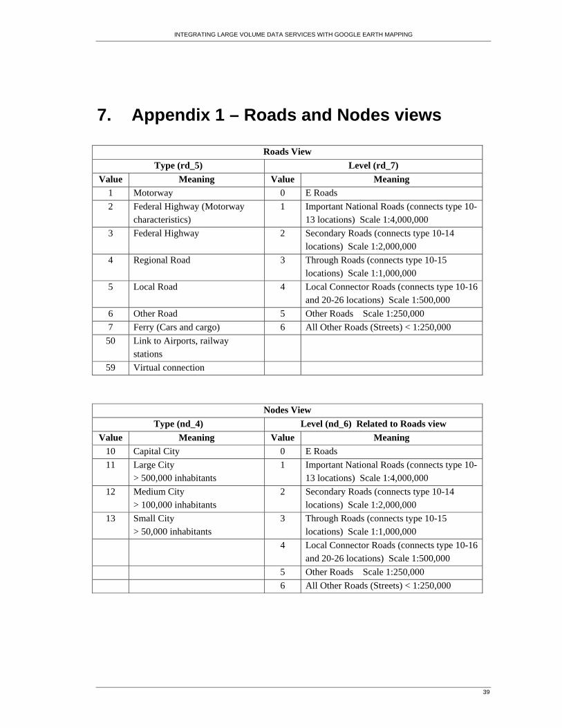
7. Appendix 1 – Roads and Nodes views
Roads View
Type (rd_5) Level (rd_7)
Value Meaning Value Meaning
1 Motorway 0 E Roads
2 Federal Highway (Motorway
characteristics)
1 Important National Roads (connects type 10-
13 locations) Scale 1:4,000,000
3 Federal Highway 2 Secondary Roads (connects type 10-14
locations) Scale 1:2,000,000
4 Regional Road 3 Through Roads (connects type 10-15
locations) Scale 1:1,000,000
5 Local Road 4 Local Connector Roads (connects type 10-16
and 20-26 locations) Scale 1:500,000
6 Other Road 5 Other Roads Scale 1:250,000
7 Ferry (Cars and cargo) 6 All Other Roads (Streets) < 1:250,000
50 Link to Airports, railway
stations
59 Virtual connection
Nodes View
Type (nd_4) Level (nd_6) Related to Roads view
Value Meaning Value Meaning
10 Capital City 0 E Roads
11 Large City
> 500,000 inhabitants
1 Important National Roads (connects type 10-
13 locations) Scale 1:4,000,000
12 Medium City
> 100,000 inhabitants
2 Secondary Roads (connects type 10-14
locations) Scale 1:2,000,000
13 Small City
> 50,000 inhabitants
3 Through Roads (connects type 10-15
locations) Scale 1:1,000,000
4 Local Connector Roads (connects type 10-16
and 20-26 locations) Scale 1:500,000
5 Other Roads Scale 1:250,000
6 All Other Roads (Streets) < 1:250,000


![Integrating Coexpression Networks with GWAS to Prioritize ... · LARGE-SCALE BIOLOGY ARTICLE Integrating Coexpression Networks with GWAS to Prioritize Causal Genes in Maize[OPEN]](https://img.pdfslide.us/doc/110x75/5f51aba08bfbac6bef7784c2/integrating-coexpression-networks-with-gwas-to-prioritize-large-scale-biology.jpg)