Gradients Weights improve Regression and Classiﬁcationskk2175/Papers/jmlr2016.pdf · c 2016 Samory Kpotufe, Abdeslam Boularias, Thomas Schultz, and Kyoungok Kim. S. KPOTUFE, A

Journal of Machine Learning Research 17 (2016) 1-34 Submitted 8/13; Revised 2/16; Published 4/16

Gradients Weights improve Regression and Classification

Samory Kpotufe∗ [email protected] University, Princeton, NJ

Abdeslam Boularias [email protected] University, New Brunswick, NJ

Thomas Schultz [email protected] of Bonn, Germany

Kyoungok Kim [email protected]

Seoul National University of Science & Technology (SeoulTech), Korea

Editor: Hui Zou

AbstractIn regression problems over Rd, the unknown function f often varies more in some coordinatesthan in others. We show that weighting each coordinate i according to an estimate of the variationof f along coordinate i – e.g. the L1 norm of the ith-directional derivative of f – is an efficientway to significantly improve the performance of distance-based regressors such as kernel and k-NN regressors. The approach, termed Gradient Weighting (GW), consists of a first pass regressionestimate fn which serves to evaluate the directional derivatives of f , and a second-pass regressionestimate on the re-weighted data. The GW approach can be instantiated for both regression andclassification, and is grounded in strong theoretical principles having to do with the way regressionbias and variance are affected by a generic feature-weighting scheme. These theoretical principlesprovide further technical foundation for some existing feature-weighting heuristics that have provedsuccessful in practice.

We propose a simple estimator of these derivative norms and prove its consistency. The pro-posed estimator computes efficiently and easily extends to run online. We then derive a classifica-tion version of the GW approach which evaluates on real-worlds datasets with as much success asits regression counterpart.Keywords: Nonparametric learning, feature selection, feature weighting, nonparametric sparsity,metric learning.

1. Introduction

High-dimensional regression is the problem of inferring an unknown function f from data pairs(Xi, Yi), i = 1, 2, . . . n, where the input Xi belongs to a Euclidean subspace X ⊂ Rd and theoutput Yi is a noisy version of f(Xi). The problem is significantly harder for larger dimension d,and various pre-processing approaches have been devised over time to alleviate this so-called curseof dimension. A simple and common approach is that of reducing the dimension of the input X byproperly selecting a few coordinate-variables with the most influence on the problem. The generalmotivating assumption for these methods is that of (approximate) sparsity: the unknown function

∗. A significant part of this work was conducted when the authors were at the Max Planck Institute for IntelligentSystems, Tuebingen, Germany.

c©2016 Samory Kpotufe, Abdeslam Boularias, Thomas Schultz, and Kyoungok Kim.

S. KPOTUFE, A. BOULARIAS, T. SCHULTZ, K. KIM

f only varies along a few relevant coordinates in some subset R of [d].= 1, 2, . . . , d, that is

f(X) = f(X(R)

)where X(R) picks out the set of relevant coordinates. However, as illustrated by

Fig. 3, there are many real-world examples in which f varies significantly along all coordinates, butvaries more in some coordinates than in others. The natural approach in this case, implicit in somemethods and heuristics (see Section 1.2), is to weight each coordinate according to some measureof relevance learned from data. The learned coordinate-relevance would typically rely on variousassumptions on the form of f , for example f might be assumed linear.

In the case of nonparametric regression, where little is assumed about the form of f , the ques-tion of how to properly weight coordinates has not received much theoretical attention. We presentand analyze a simple approach termed Gradient Weighting (GW), consisting of weighting each co-ordinate i according to the (unknown) variation of f along i. To this end, f is estimated from datain a first pass as fn, where fn serves to assess the coordinate-wise variation of f and accordinglyweight the data; the transformed data is then used to re-estimate f in a second pass. This proce-dure can be iterated into a multi-pass procedure, although we only consider the two-pass versionjust described. We show that such weighting can be learned efficiently, is easily extended online,and can significantly improve the performance of distance-based regressors (e.g. kernel and k-NNregression) in real-world applications. Moreover the method easily extends to distance-based clas-sification methods such as k-NN classification and ε-NN classification.

The GW approach is grounded in strong theoretical principles (developed in Section 2) havingto do with the way regression bias and variance are affected by the distribution of weights in ageneric feature-weighting method. We argue in Section 2 that a good situation for distance-basedregressors is one where the unknown function f varies in a few coordinates more than in others, andthe weights correlate with the variation of f along coordinates. The theoretical intuition developedis kept general enough to also explain the practical success of some existing heuristics (see Section6.2) which inherently learn weights that are correlated with the variation of the unknown f alongcoordinates. We validate the theoretical intuition in extensive experiments on many real-worlddatasets in Section 5.

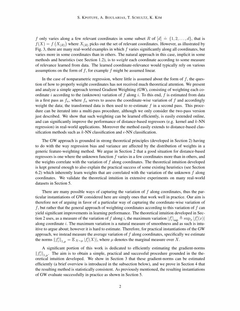
There are many possible ways of capturing the variation of f along coordinates, thus the par-ticular instantiations of GW considered here are simply ones that work well in practice. Our aim istherefore not of arguing in favor of a particular way of capturing the coordinate-wise variation off , but rather that the general approach of weighting coordinates according to this variation of f canyield significant improvements in learning performance. The theoretical intuition developed in Sec-tion 2 uses, as a measure of the variation of f along i, the maximum variation |f ′i |sup , supx |f ′i(x)|along coordinate i. The maximum variation is a natural measure of smoothness and as such is intu-itive to argue about; however it is hard to estimate. Therefore, for practical instantiations of the GWapproach, we instead measure the average variation of f along coordinates, specifically we estimatethe norms ‖f ′i‖1,µ = EX∼µ |f ′i(X)|, where µ denotes the marginal measure over X .

A significant portion of this work is dedicated to efficiently estimating the gradient-norms‖f ′i‖1,µ. The aim is to obtain a simple, practical and successful procedure grounded in the the-oretical intuition developed. We show in Section 3 that these gradient-norms can be estimatedefficiently (a brief overview is introduced in the subsection below), and we prove in Section 4 thatthe resulting method is statistically consistent. As previously mentioned, the resulting instantiationsof GW evaluate successfully in practice as shown in Section 5.

2

GRADIENTS WEIGHTS

1.1 GW for distance-based nonparametric methods

For distance-based methods, the weights can be incorporated into a distance function of the form

ρ(x, x′) ,(

(x− x′)>W(x− x′))1/2

, (1)

where each element Wi of the diagonal matrix W is an estimate of the variation of f along coor-dinate i, as captured for instance by ‖f ′i‖1,µ. In our evaluations we set Wi to an estimate ∇n,i of‖f ′i‖1,µ, or to the square estimate∇2

n,i.To estimate ‖f ′i‖1,µ, one does not need to estimate f ′i well everywhere, just well on average.

While many elaborate derivative estimators exist (see e.g. (Hardle and Gasser, 1985)), we have tokeep in mind our need for a fast but consistent estimator of ‖f ′i‖1,µ. We propose a simple estimator∇n,i which averages the differences along i of an estimator fn,h of f . More precisely (see Section 3)∇n,i has the form En |fn,h(X + tei)− fn,h(X − tei)| /2t where En denotes empirical expectationover a sample Xin1 . ∇n,i can therefore be updated online at the cost of just two estimates of fn,h,given a proper online version of fn,h (see e.g. Gu and Lafferty (2012)).

In this paper fn,h is a kernel estimator, although any regression method might be used in esti-mating ‖f ′i‖1,µ. We prove in Section 4 that, under mild conditions, Wi is a consistent estimator ofthe unknown norm ‖f ′i‖1,µ. Moreover we prove finite sample convergence bounds to help guide thepractical tuning of the two parameters t and h.

1.2 Related Work

The GW approach is close in spirit to metric learning (Weinberger and Tesauro, 2007; Xiao et al.,2009; Shalev-shwartz et al., 2004; Davis et al., 2007), where the best metric ρ is found by optimizingover a sufficiently large space of possible metrics. Clearly metric learning can only yield betterperformance, but the optimization over a larger space will result in heavier preprocessing time,often O(n2) on datasets of size n. Yet, preprocessing time is especially important in many modernapplications where data sizes are large, or where training and prediction have real-time constraints(e.g. robotics, finance, advertisement, recommendation systems). Here we do not optimize overa space of metrics, but rather estimate a single metric ρ based on the coordinate-wise variation off . Our metric ρ is efficiently obtained, can be estimated online, and still significantly improves theperformance of distance-based regressors.

We also note that there are actually few metric learning approaches for regression and these aretypically designed around a particular regression approach or problem. The method by Weinbergerand Tesauro (2007) is designed for Gaussian-kernel regression, the one by Xiao et al. (2009) is tunedto the particular problem of age estimation. For the problem of classification, the metric-learningapproaches of Shalev-shwartz et al. (2004); Davis et al. (2007) are meant for online applications –they are therefore relatively efficient methods – but cannot be used in regression.

In the case of kernel regression and local polynomial regression, multiple bandwidths can beused, one for each coordinate. However, tuning d bandwidth parameters requires searching a d-dimensional grid, i.e. the number of possible settings is exponential in d, which is impractical evenin batch mode. The RODEO method of Lafferty and Wasserman (2005) alleviates this problem,however only in the particular case of local linear regression. Our method applies to any distance-based regressor.

The ideas presented here are related to recent notions of nonparametric sparsity where it isassumed that the target function is well approximated by a sparse function, i.e. one which varies in

3


just a few coordinates (e.g. Hoffmann and Lepski (2002); Lafferty and Wasserman (2005); Rigolletand Tsybakov (2011); Rosasco et al. (2012)). The method of Rosasco et al. (2012) is most relatedto the present work in that they employ a penalized learning objective based on the coordinate-wisevariation of f , as captured by the L2 gradient norms ‖f ′i‖2,µ. However, as in the other works onsparsity just mentioned, Rosasco et al. (2012) relies on f being actually sparse or at least close tosparse. In the present work we do not need sparsity, instead we only need the target function f tovary in some coordinates more than in others which is most likely the case in practice. Our approachtherefore works in practice even in cases where the target function is far from sparse.

One line of work which also does away with the assumption of sparsity of f , is that of anisotropicregression (Nusbaum (1983); Hoffmann and Lepski (2002)). Anisotropic regression assumes thatthe target function f does not have the same degree of smoothness in all coordinate directions,where smoothness is roughly captured by the number of bounded derivatives of f . The attainablerates in anisotropic regression are better than the usual minimax rates for nonparametric regression(e.g. Stone (1980)) which consider the worst-case degree of smoothness across all coordinates. Inthe present work, we only consider the first derivatives of f across coordinates, in other words f isallowed to have the same degree of smoothness across coordinates, but we are interested in the casewhere these coordinate-wise derivatives have different magnitudes. We show in Section 2 that thisis enough to attain better rates than the usual minimax rates, in particular by using the GW approachproposed here.

As previously mentioned, the theoretical intuition developed in this work helps explain thepractical success of some existing heuristics. In particular the popular Relief family of heuristics(e.g. Kira and Rendell (1992); Kononenko (1994); Robnik-Sikonja and Kononenko (2003)) canbe viewed as inherently learning weights that are correlated with the coordinate-wise variation off . Our work therefore offers new insights about existing heuristics and opens possible avenues offurther development of these heuristics. This theme is further developed in Section 6.2.

Finally, part of this work appeared as a conference version Kpotufe and Boularias (2012) cov-ering the case of regression. The present work covers both regression and classification and furtherdiffers in the technical motivation offered for the GW approach. While Kpotufe and Boularias(2012) argues for GW under strong uniform assumptions on the marginal distribution µ on X , thetheoretical intuition developed in the present work assumes a general distribution µ. The more gen-eral assumptions are made possible by introducing a new set of techniques dealing with the coveringnumbers of the space X after data weighting.

1.3 Paper Outline

In summary, we develop theoretical intuition for GW in Section 2. In Section 3 we derive a concretemethod for estimating the coordinate-wise variablity of f ; the method is both simple and efficient.We show in Section 4 that the method is a consistent estimator of the gradient norms ‖f ′i‖1,µ.In Section 5 we validate our theory on various real-world applications. We finish with a generaldiscussion of our results in Section 6, including possible future directions.

2. Theoretical Justification of GW

In this section we develop theoretical intuition about why GW works. We focus on the problem ofnonparametric regression since the same intuition is easily implied for the case of nonparametricclassification (see Section 2.3). We will argue that it is possible to attain good regression rates

4

GRADIENTS WEIGHTS

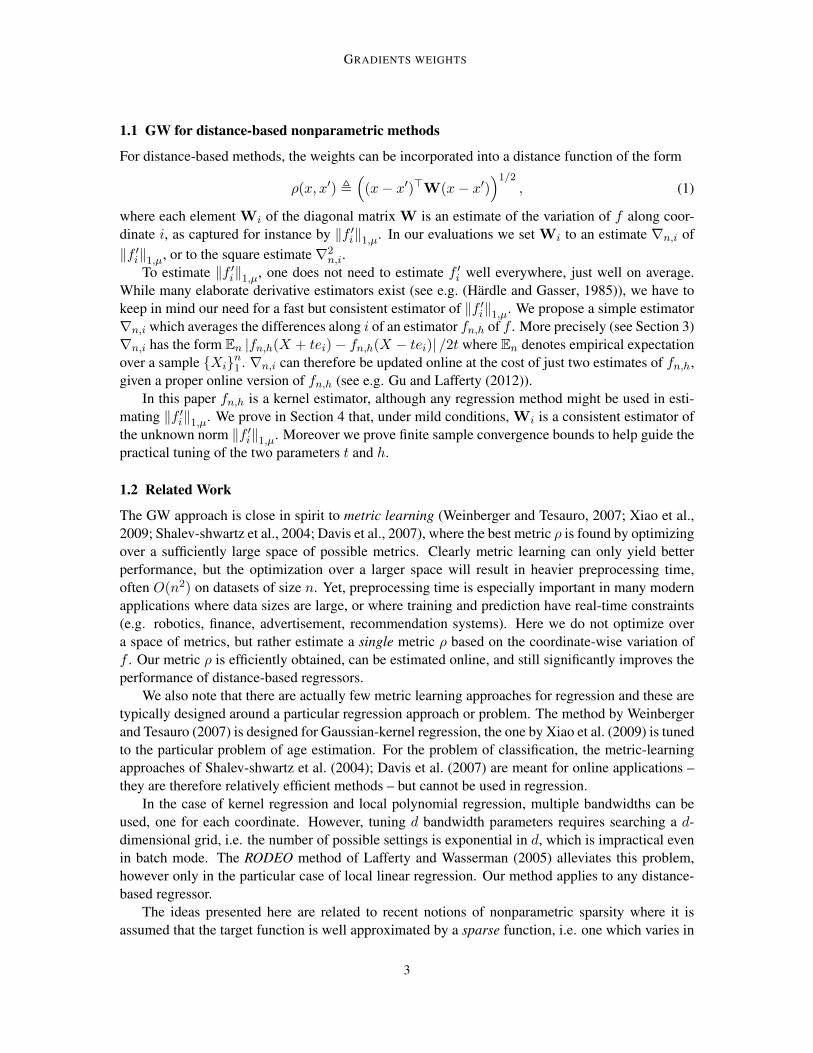
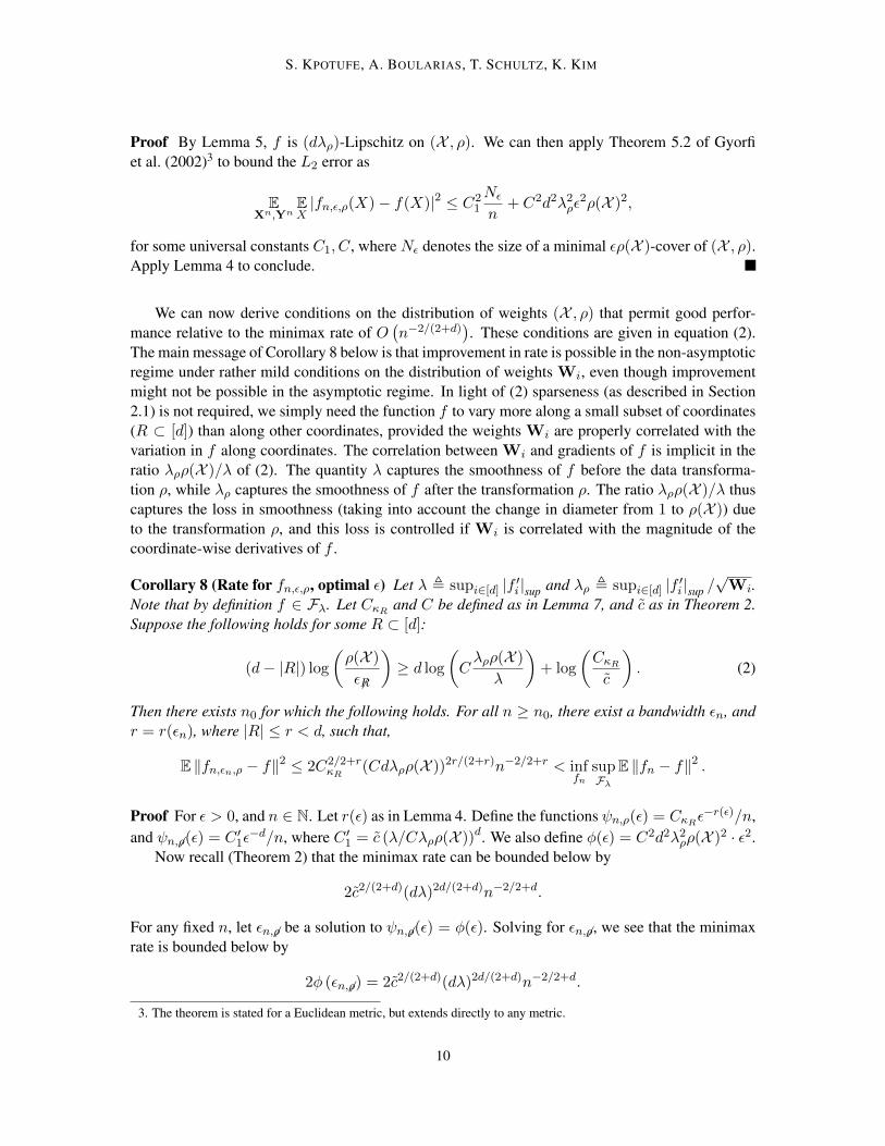
Figure 1: Illustration of a sparse function. Here x = (x1, x2), and f (x) = f (x2). There is novariation in f along coordinate 1, in other words |f ′1|sup = 0 and ‖f ′1‖1,µ = 0.

even when the target function f depends on all coordinates, provided f does not vary equally inall coordinates, and the gradient weights Wi are correlated with the coordinate-wise variation inf . The coordinate-wise variation will be captured in this discussion by the quantities |f ′i |sup ,supx∈X |f ′i(x)|, i ∈ [d], as previously mentioned.

We will consider the metric ρ generally: instead of assuming a particular form, we will let theanalysis uncover a form of ρ which yields improved regression rates. Improvement is measuredhere in a minimax sense which will soon be made clear. The analysis of this section will thus yieldintuition not only about GW, but about coordinate-weighting generally.

We have the following assumption throughout the section.

Assumption 2.1 The input space X is full-dimensional in Rd, connected1, and has bounded diam-eter ‖X‖ , supx,x′∈X ‖x− x′‖ = 1. The output space is Y = [0, 1].

2.1 Rough Intuition: the sparse case

We start with a simple case where the unknown function is actually R-sparse, i.e. depends on asmall set of coordinates R ( [d] (illustrated in Figure 2.1). The function f then varies only alongcoordinates in R, i.e. f ′i 6= 0 only for coordinates i ∈ R. Hence if the metric ρ is defined by settingthe gradient weights Wi to either |f ′i |sup and ‖f ′i‖1,µ, the resulting space (X , ρ) is a (weighted) pro-jection of the original Euclidean X down to just the relevant coordinates R ( [d]. Thus regressionor classification on (X , ρ) would have performance depending on the lower-dimension |R| of thisspace, rather than the high-dimension d of the original space.

To make this intuition precise, we introduce the following definition and minimax theorem.

Definition 1 (The class Fλ) Given λ > 0, we let Fλ denote all distributions PX,Y on X × [0, 1]such that, for all i ∈ [d], the directional derivatives of f(x) , E [Y |X = x] satisfy |f ′i |sup ,supx∈X |f ′i(x)| ≤ λ.

The worst-case rate for the class Fλ is given in the following minimax theorem of Stone.

Theorem 2 (Minimax rate for Fλ: Stone (1982)) There exists c < 1, independent of n, such thatfor all sample sizes n ∈ N,

inffn

supf∈Fλ

EXn,Yn

‖fn − f‖2 ≥ 2c2/(2+d)(dλ)2d/(2+d)n−2/2+d,

1. This is needed so that ‖f ′i‖1,µ = 0 implies that f is a.e. constant along coordinate i.

5


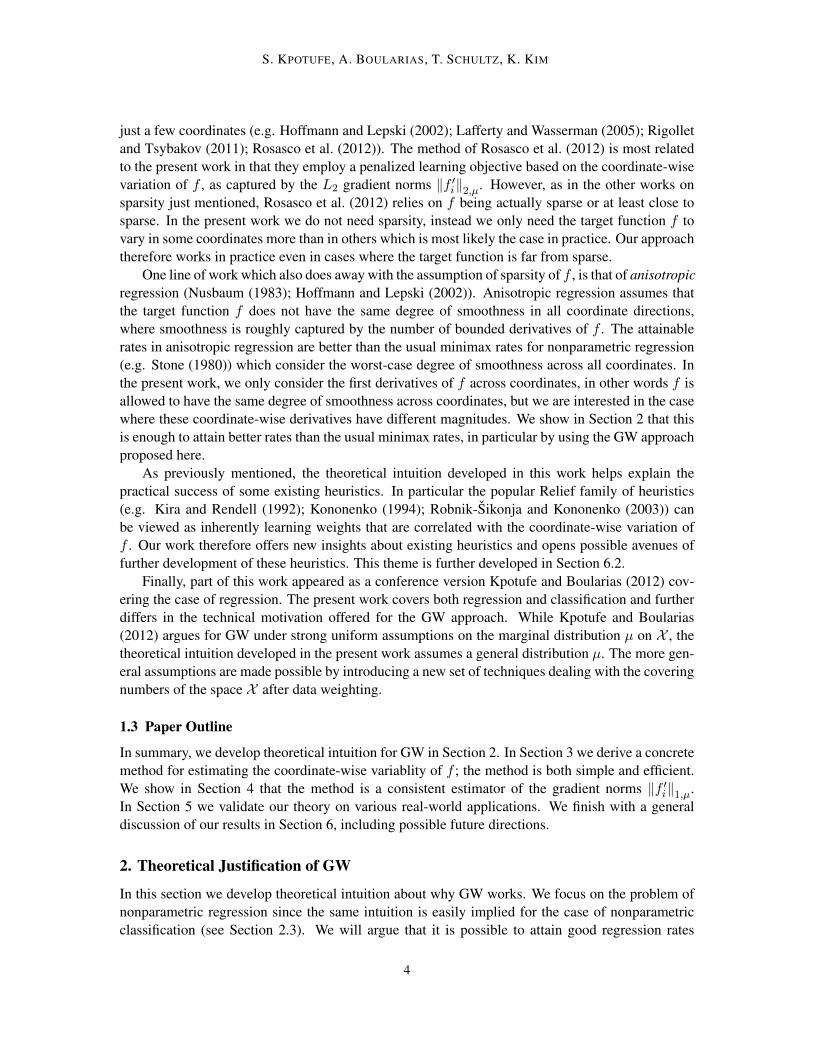
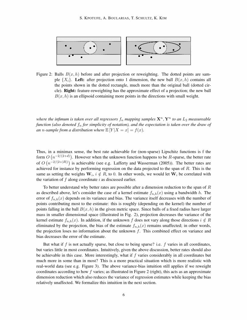
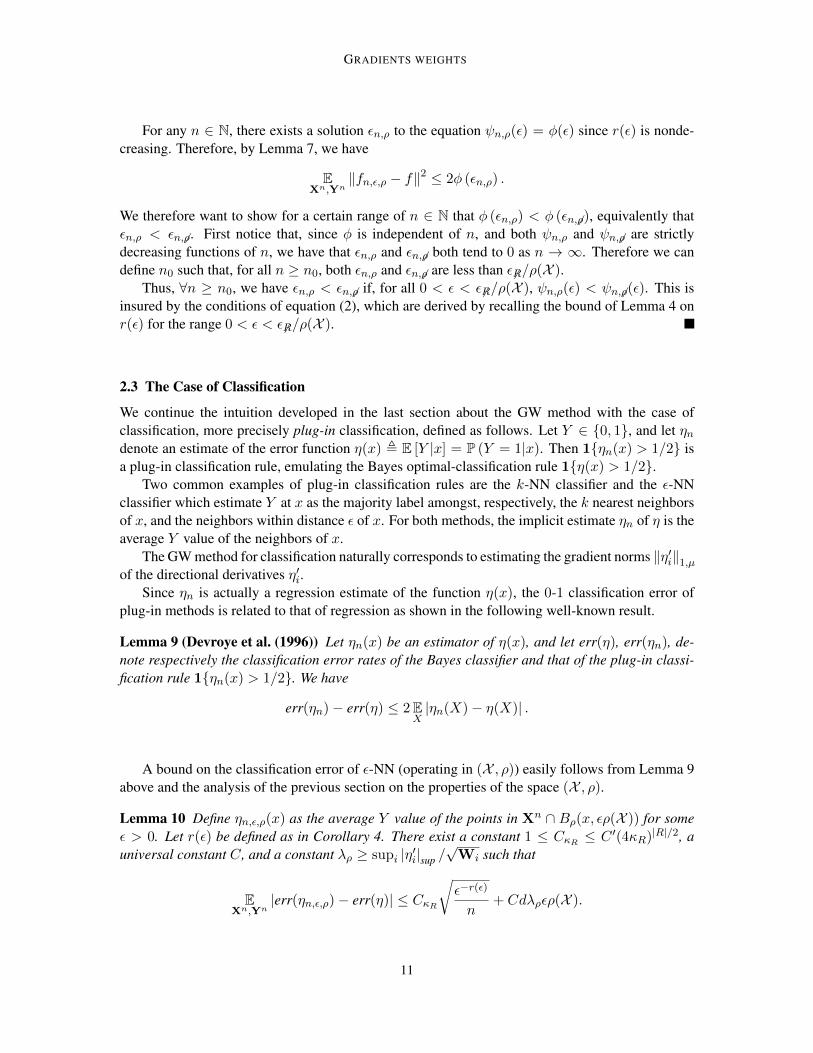
Figure 2: Balls B(x, h) before and after projection or reweighting. The dotted points are sam-ple Xi. Left: after projection onto 1 dimension, the new ball B(x, h) contains allthe points shown in the dotted rectangle, much more than the original ball (dotted cir-cle). Right: feature-reweighting has the approximate effect of a projection; the new ballB(x, h) is an ellipsoid containing more points in the directions with small weight.

where the infimum is taken over all regressors fn mapping samples Xn,Yn to an L2 measureablefunction (also denoted fn for simplicity of notation), and the expectation is taken over the draw ofan n-sample from a distribution where E [Y |X = x] = f(x).

Thus, in a minimax sense, the best rate achievable for (non-sparse) Lipschitz functions is f theform O

(n−2/(2+d)

). However when the unknown function happens to be R-sparse, the better rate

of O(n−2/(2+|R|)) is achievable (see e.g. Lafferty and Wasserman (2005)). The better rates are

achieved for instance by performing regression on the data projected to the span of R. This is thesame as setting the weights Wi, i /∈ R, to 0. In other words, we would let Wi be correlated withthe variation of f along coordinate i as discussed earlier.

To better understand why better rates are possible after a dimension reduction to the span of Ras described above, let’s consider the case of a kernel estimate fn,h(x) using a bandwidth h. Theerror of fn,h(x) depends on its variance and bias. The variance itself decreases with the number ofpoints contributing most to the estimate: this is roughly (depending on the kernel) the number ofpoints falling in the ball B(x, h) in the given metric space. Since balls of a fixed radius have largermass in smaller dimensional space (illustrated in Fig. 2), projection decreases the variance of thekernel estimate fn,h(x). In addition, if the unknown f does not vary along those directions i /∈ Reliminated by the projection, the bias of the estimate fn,h(x) remains unaffected; in other words,the projection loses no information about the unknown f . This combined effect on variance andbias decreases the error of the estimate.

But what if f is not actually sparse, but close to being sparse? i.e. f varies in all coordinates,but varies little in most coordinates. Intuitively, given the above discussion, better rates should alsobe achievable in this case. More interestingly, what if f varies considerably in all coordinates butmuch more in some than in most? This is a more practical situation which is more realistic withreal-world data (see e.g. Figure 3). The above variance-bias intuition still applies if we reweightcoordinates according to how f varies; as illustrated in Figure 2 (right), this acts as an approximatedimension reduction which also reduces the variance of regression estimates while keeping the biasrelatively unaffected. We formalize this intuition in the next section.

6

GRADIENTS WEIGHTS

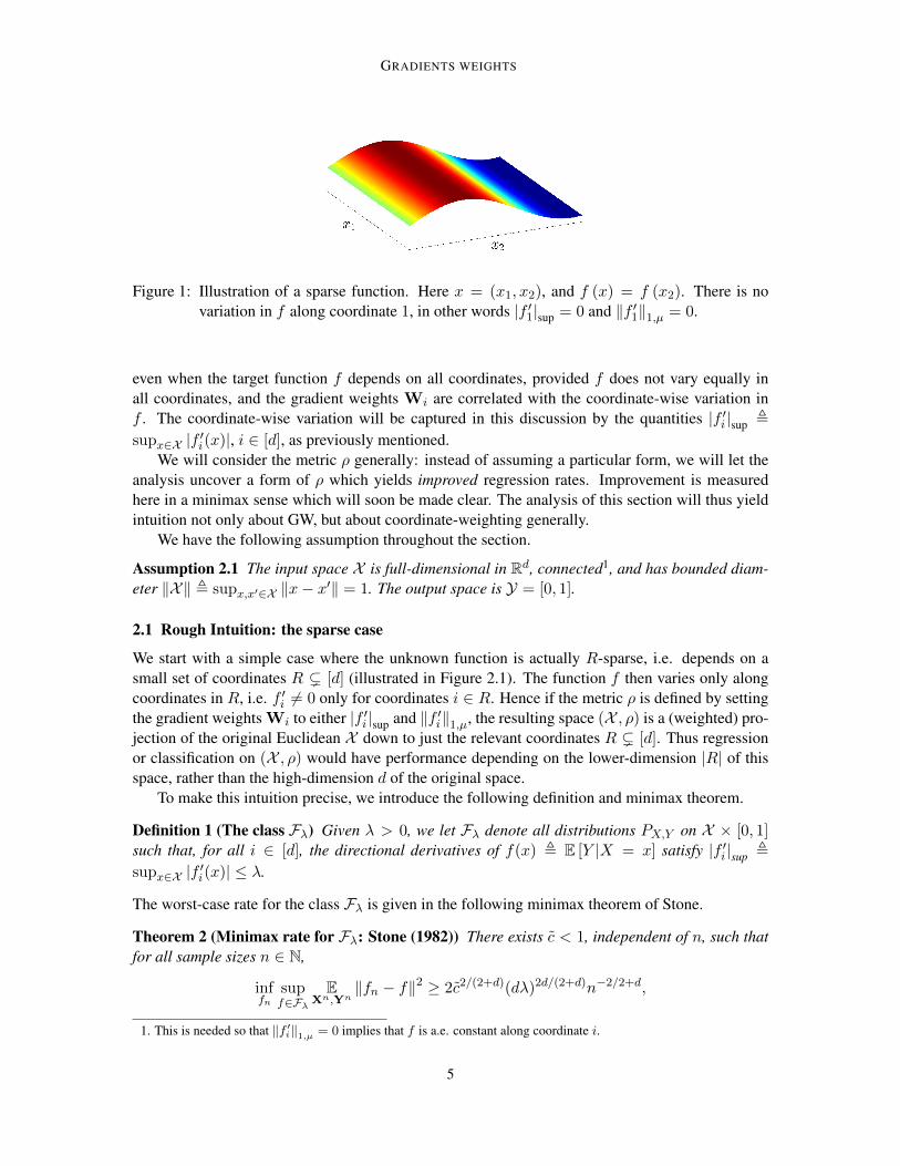
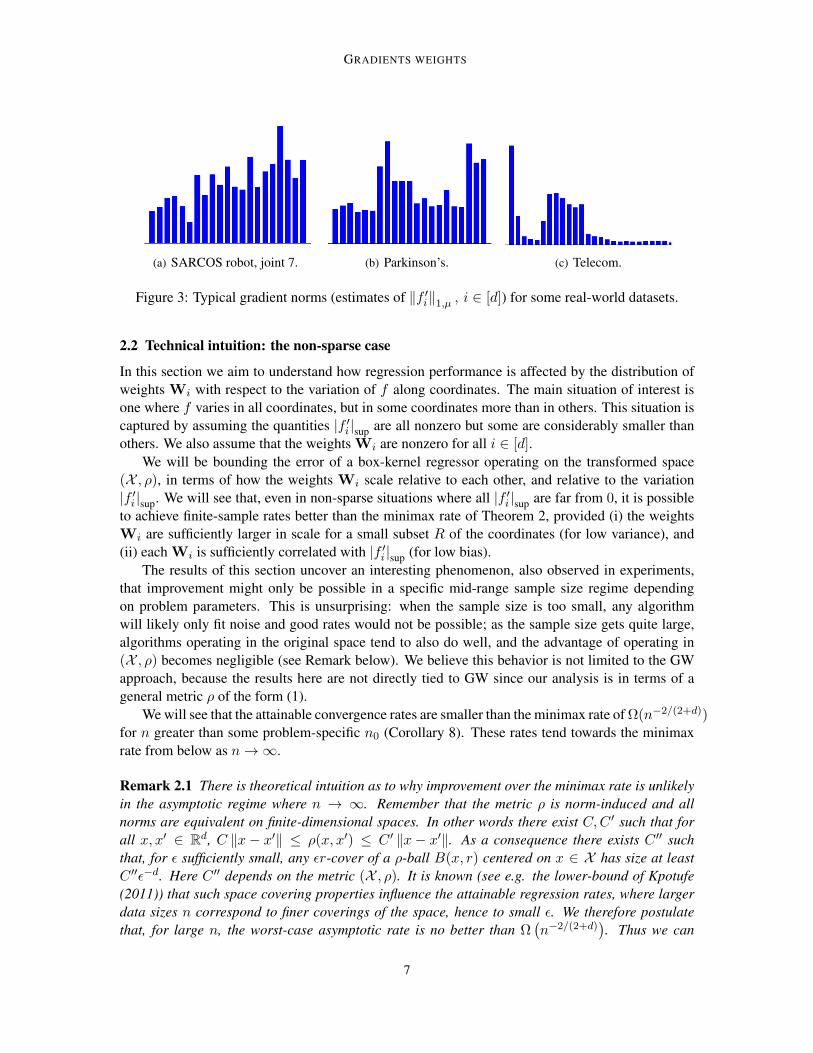
(a) SARCOS robot, joint 7. (b) Parkinson’s. (c) Telecom.

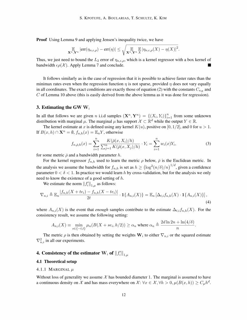
Figure 3: Typical gradient norms (estimates of ‖f ′i‖1,µ , i ∈ [d]) for some real-world datasets.

2.2 Technical intuition: the non-sparse case

In this section we aim to understand how regression performance is affected by the distribution ofweights Wi with respect to the variation of f along coordinates. The main situation of interest isone where f varies in all coordinates, but in some coordinates more than in others. This situation iscaptured by assuming the quantities |f ′i |sup are all nonzero but some are considerably smaller thanothers. We also assume that the weights Wi are nonzero for all i ∈ [d].

We will be bounding the error of a box-kernel regressor operating on the transformed space(X , ρ), in terms of how the weights Wi scale relative to each other, and relative to the variation|f ′i |sup. We will see that, even in non-sparse situations where all |f ′i |sup are far from 0, it is possibleto achieve finite-sample rates better than the minimax rate of Theorem 2, provided (i) the weightsWi are sufficiently larger in scale for a small subset R of the coordinates (for low variance), and(ii) each Wi is sufficiently correlated with |f ′i |sup (for low bias).

The results of this section uncover an interesting phenomenon, also observed in experiments,that improvement might only be possible in a specific mid-range sample size regime dependingon problem parameters. This is unsurprising: when the sample size is too small, any algorithmwill likely only fit noise and good rates would not be possible; as the sample size gets quite large,algorithms operating in the original space tend to also do well, and the advantage of operating in(X , ρ) becomes negligible (see Remark below). We believe this behavior is not limited to the GWapproach, because the results here are not directly tied to GW since our analysis is in terms of ageneral metric ρ of the form (1).

We will see that the attainable convergence rates are smaller than the minimax rate of Ω(n−2/(2+d))for n greater than some problem-specific n0 (Corollary 8). These rates tend towards the minimaxrate from below as n→∞.

Remark 2.1 There is theoretical intuition as to why improvement over the minimax rate is unlikelyin the asymptotic regime where n → ∞. Remember that the metric ρ is norm-induced and allnorms are equivalent on finite-dimensional spaces. In other words there exist C,C ′ such that forall x, x′ ∈ Rd, C ‖x− x′‖ ≤ ρ(x, x′) ≤ C ′ ‖x− x′‖. As a consequence there exists C ′′ suchthat, for ε sufficiently small, any εr-cover of a ρ-ball B(x, r) centered on x ∈ X has size at leastC ′′ε−d. Here C ′′ depends on the metric (X , ρ). It is known (see e.g. the lower-bound of Kpotufe(2011)) that such space covering properties influence the attainable regression rates, where largerdata sizes n correspond to finer coverings of the space, hence to small ε. We therefore postulatethat, for large n, the worst-case asymptotic rate is no better than Ω

(n−2/(2+d)

). Thus we can

7


only expect improvements over the minimax rate in small sample regimes, where small is problem-specific. Note that this remark is of independent interest since other approaches such as metriclearning would typically use norm-induced metrics.

The analysis in this section, although focusing on kernel regression, yields general intuitionabout the behavior of other related distance-based regressors such as k-NN, since such regressorsare similarly affected by characteristics of the regression problem (e.g. smoothness of f , intrinsicdimension of (X , ρ)).

We start by defining quantities which serve to describe the distribution of weights Wi.

Definition 3 For any subset of coordinates R ⊂ [d], define κR ,√

maxi∈RWi/mini∈RWi, andlet ε6R , 2

√maxi/∈RWi. Finally we define the ρ-diameter of X as ρ(X ) , supx,x′∈X ρ(x, x′).

As discussed earlier, regression variance is small if there exists a small subset R for which theweights Wi are relatively larger than those for coordinates not in R. Formally, we want the quanti-ties |R|, ε6R and κR relatively small for some R ⊂ [d]. How small will become gradually clearer.

We start with two results (Lemmas 4 and 5 below) on properties of the metric space (X , ρ)which affect the behavior of a distance-based regressor such as fn,ε,ρ. All omitted proofs are givenin the appendix.

The first Lemma 4 concerns the size of minimal covers (at different scales) of the metric (X , ρ).Such cover sizes influence the variance of a distance-based regressor operating on (X , ρ). If (X , ρ)has small cover-sizes, it can typically be covered by large balls, each ball likely to contain enoughdata for small regression variance. Lemma 4 roughly states that, while a minimal ε-cover of theEuclidean space X ⊂ Rd has size O

(ε−d), an ερ(X )-cover of (X , ρ) has smaller size Cε−r where

|R| ≤ r ε→0−−→ d. Both C and the function r(ε) depend on the relative distribution of weights Wi ascaptured by the quantities |R|, ε6R and κR.

Lemma 4 (Covering numbers) Consider R ⊂ [d] such that maxi/∈RWi < mini∈RWi. Thereexist C ≤ C ′(4κR)|R| such that, for any ε > 0, the smallest ερ(X )-cover of (X , ρ) has size at mostCε−r(ε), where r(ε) is a nondecreasing function of ε satisfying

r(ε) ≤

|R| if ε ≥ ε6R/ρ(X )

d− (d− |R|) · log(ρ(X )/ε6R)log(1/ε) if ε < ε6R/ρ(X )

The function r(ε) captures the dimension of (X , ρ)2. We thus want r to be small so that the transfor-mation ρ acts like a low-dimensional projection and hence helps reduce variance. The function r issmallest when most weights are concentrated in a small subset R, i.e. we want small |R| and smallε6R/ρ(X ) (this term captures the difference in magnitude between weights not in R and weights inR). It might therefore seem preferable to choose ρ in this way, but we have to be careful: not alldimension reduction is good since such a transformation ρ might introduce additional regressionbias. We therefore need to understand how regression bias is affected by the distribution of weightsWi in the transformation ρ.

Lemma 5 below captures the smoothness properties of the target function f in the transformedmetric (X , ρ). These smoothness properties affect the bias of distance-based regressors on (X , ρ).

2. The logarithm of covering numbers is a common measure of metric dimension, see e.g. Clarkson (2005) for anoverview of the subject.

8

GRADIENTS WEIGHTS

Lemma 5 (Change in Lipschitz smoothness for f ) Suppose each derivative f ′i is bounded on Xby |f ′i |sup. Assume Wi > 0 whenever |f ′i |sup > 0. Denote by R the largest subset of [d] such that|f ′i |sup > 0 for i ∈ R . We have for all x, x′ ∈ X ,

∣∣f(x)− f(x′)∣∣ ≤ (∑

i∈R

|f ′i |sup√Wi

)ρ(x, x′).

We want f to be as smooth as possible, in other words we want the Lipschitz parameter(∑i∈R|f ′i|sup√

Wi

)as small as possible. Suppose Wi is uncorrelated with the variation of f along

i, e.g. Wi is small for those coordinates where |f ′i |sup is large, then the function f might end uplacking smoothness in the modified space (X , ρ). While it is hard to estimate |f ′i |sup, we can ex-pect it to be correlated with ‖f ′i‖1,µ which is easier to estimate (Section 3). Thus by keeping theweights Wi correlated with the gradient norms ‖f ′i‖1,µ, we expect the function f to remain rela-tively smooth in the space (X , ρ) and hence we expect to maintain control on regression bias. Sinceit is unlikely in practice that f varies equally in all coordinates (Figure 3), in light of Lemma 20,we will expect better regression performance in the space (X , ρ) as variance should decrease whilebias remains controlled.

Remark 2.2 As previously mentioned, there are many ways to incorporate the coordinate-wisevariability of f into the weights ρ, and GW (or Relief heuristics discussed in Section 6.2) is just

one of this. In light of the Lipschitz parameter(∑

i∈R|f ′i|sup√

Wi

), we could reasonably set Wi to

approximate ‖f ′i‖q1,µ for some q > 0 (q = 1, 2 in this work), or to ‖f ′i‖

qi1,µ for some power qi

depending on i. These are interesting questions deserving further investigation.

We now go further in formalizing the intuition discussed so far by considering the case of kernelregression in (X , ρ). We will derive exact conditions on the distribution of weights Wi that allowimprovements over the minimax rate of O

(n−2/(2+d)

)in the non-asymptotic regime.

The box-kernel regression estimate is defined as follows.

Definition 6 Given ε > 0 and x ∈ X , the box-kernel estimate at x is defined as follows. Recall thatρ(X ) , supx,x′∈X ρ(x, x′) denotes the ρ-diameter of X :

fn,ε,ρ(x) , average Yi of points Xi ∈ B(x, ερ(X )), or 0 if B(x, ερ(X )) is empty.

The next lemma establishes the convergence rate for a box-kernel regressor using any given band-width ερ(X ). The lemma is a simple application of known results on the bias and variance ofa kernel regressor combined with the previous two lemmas on the dimension of (X , ρ) and thesmoothnness of f on (X , ρ).

Lemma 7 (Rate for fn,ε,ρ, arbitrary ε) Consider anyR ⊂ [d] such that maxi/∈RWi < mini∈RWi.There exist 1 ≤ CκR ≤ C ′(4κR)|R|, a universal constant C, and λρ ≥ supi |f ′i |sup /

√Wi such that

EXn,Yn

|fn,ε,ρ − f |2 ≤ CκRε−r(ε)

n+ C2d2λ2

ρε2ρ(X )2,

where r(ε) is defined as in Lemma 4.

9


Proof By Lemma 5, f is (dλρ)-Lipschitz on (X , ρ). We can then apply Theorem 5.2 of Gyorfiet al. (2002)3 to bound the L2 error as

EXn,Yn

EX|fn,ε,ρ(X)− f(X)|2 ≤ C2

1

Nε

n+ C2d2λ2

ρε2ρ(X )2,

for some universal constants C1, C, where Nε denotes the size of a minimal ερ(X )-cover of (X , ρ).Apply Lemma 4 to conclude.

We can now derive conditions on the distribution of weights (X , ρ) that permit good perfor-mance relative to the minimax rate of O

(n−2/(2+d)

). These conditions are given in equation (2).

The main message of Corollary 8 below is that improvement in rate is possible in the non-asymptoticregime under rather mild conditions on the distribution of weights Wi, even though improvementmight not be possible in the asymptotic regime. In light of (2) sparseness (as described in Section2.1) is not required, we simply need the function f to vary more along a small subset of coordinates(R ⊂ [d]) than along other coordinates, provided the weights Wi are properly correlated with thevariation in f along coordinates. The correlation between Wi and gradients of f is implicit in theratio λρρ(X )/λ of (2). The quantity λ captures the smoothness of f before the data transforma-tion ρ, while λρ captures the smoothness of f after the transformation ρ. The ratio λρρ(X )/λ thuscaptures the loss in smoothness (taking into account the change in diameter from 1 to ρ(X )) dueto the transformation ρ, and this loss is controlled if Wi is correlated with the magnitude of thecoordinate-wise derivatives of f .

Corollary 8 (Rate for fn,ε,ρ, optimal ε) Let λ , supi∈[d] |f ′i |sup and λρ , supi∈[d] |f ′i |sup /√Wi.

Note that by definition f ∈ Fλ. Let CκR and C be defined as in Lemma 7, and c as in Theorem 2.Suppose the following holds for some R ⊂ [d]:

(d− |R|) log

(ρ(X )

ε6R

)≥ d log

(Cλρρ(X )

λ

)+ log

(CκRc

). (2)

Then there exists n0 for which the following holds. For all n ≥ n0, there exist a bandwidth εn, andr = r(εn), where |R| ≤ r < d, such that,

E ‖fn,εn,ρ − f‖2 ≤ 2C2/2+r

κR(Cdλρρ(X ))2r/(2+r)n−2/2+r < inf

fnsupFλ

E ‖fn − f‖2 .

Proof For ε > 0, and n ∈ N. Let r(ε) as in Lemma 4. Define the functions ψn,ρ(ε) = CκRε−r(ε)/n,

and ψn,6ρ(ε) = C ′1ε−d/n, where C ′1 = c (λ/Cλρρ(X ))d. We also define φ(ε) = C2d2λ2

ρρ(X )2 · ε2.Now recall (Theorem 2) that the minimax rate can be bounded below by

2c2/(2+d)(dλ)2d/(2+d)n−2/2+d.

For any fixed n, let εn, 6ρ be a solution to ψn,6ρ(ε) = φ(ε). Solving for εn,6ρ, we see that the minimaxrate is bounded below by

2φ (εn,6ρ) = 2c2/(2+d)(dλ)2d/(2+d)n−2/2+d.

3. The theorem is stated for a Euclidean metric, but extends directly to any metric.

10

GRADIENTS WEIGHTS

For any n ∈ N, there exists a solution εn,ρ to the equation ψn,ρ(ε) = φ(ε) since r(ε) is nonde-creasing. Therefore, by Lemma 7, we have

EXn,Yn

‖fn,ε,ρ − f‖2 ≤ 2φ (εn,ρ) .

We therefore want to show for a certain range of n ∈ N that φ (εn,ρ) < φ (εn, 6ρ), equivalently thatεn,ρ < εn,6ρ. First notice that, since φ is independent of n, and both ψn,ρ and ψn, 6ρ are strictlydecreasing functions of n, we have that εn,ρ and εn, 6ρ both tend to 0 as n → ∞. Therefore we candefine n0 such that, for all n ≥ n0, both εn,ρ and εn, 6ρ are less than ε6R/ρ(X ).

Thus, ∀n ≥ n0, we have εn,ρ < εn,6ρ if, for all 0 < ε < ε 6R/ρ(X ), ψn,ρ(ε) < ψn, 6ρ(ε). This isinsured by the conditions of equation (2), which are derived by recalling the bound of Lemma 4 onr(ε) for the range 0 < ε < ε 6R/ρ(X ).

2.3 The Case of Classification

We continue the intuition developed in the last section about the GW method with the case ofclassification, more precisely plug-in classification, defined as follows. Let Y ∈ 0, 1, and let ηndenote an estimate of the error function η(x) , E [Y |x] = P (Y = 1|x). Then 1ηn(x) > 1/2 isa plug-in classification rule, emulating the Bayes optimal-classification rule 1η(x) > 1/2.

Two common examples of plug-in classification rules are the k-NN classifier and the ε-NNclassifier which estimate Y at x as the majority label amongst, respectively, the k nearest neighborsof x, and the neighbors within distance ε of x. For both methods, the implicit estimate ηn of η is theaverage Y value of the neighbors of x.

The GW method for classification naturally corresponds to estimating the gradient norms ‖η′i‖1,µof the directional derivatives η′i.

Since ηn is actually a regression estimate of the function η(x), the 0-1 classification error ofplug-in methods is related to that of regression as shown in the following well-known result.

Lemma 9 (Devroye et al. (1996)) Let ηn(x) be an estimator of η(x), and let err(η), err(ηn), de-note respectively the classification error rates of the Bayes classifier and that of the plug-in classi-fication rule 1ηn(x) > 1/2. We have

err(ηn)− err(η) ≤ 2EX|ηn(X)− η(X)| .

A bound on the classification error of ε-NN (operating in (X , ρ)) easily follows from Lemma 9above and the analysis of the previous section on the properties of the space (X , ρ).

Lemma 10 Define ηn,ε,ρ(x) as the average Y value of the points in Xn ∩ Bρ(x, ερ(X )) for someε > 0. Let r(ε) be defined as in Corollary 4. There exist a constant 1 ≤ CκR ≤ C ′(4κR)|R|/2, auniversal constant C, and a constant λρ ≥ supi |η′i|sup /

√Wi such that

EXn,Yn

|err(ηn,ε,ρ)− err(η)| ≤ CκR

√ε−r(ε)

n+ Cdλρερ(X ).

11


Proof Using Lemma 9 and applying Jensen’s inequality twice, we have

EXn,Yn

|err(ηn,ε,ρ)− err(η)| ≤√

EXn,Yn

EX|ηn,ε,ρ(X)− η(X)|2.

Thus, we just need to bound the L2 error of ηn,ε,ρ, which is a kernel regressor with a box kernel ofbandwidth ερ(X ). Apply Lemma 7 and conclude.

It follows similarly as in the case of regression that it is possible to achieve faster rates than theminimax rates even when the regression function η is not sparse, provided η does not vary equallyin all coordinates. The exact conditions are exactly those of equation (2) with the constants CκR andC of Lemma 10 above (this is easily derived from the above lemma as it was done for regression).

3. Estimating the GW Wi

In all that follows we are given n i.i.d samples (Xn,Yn) = (Xi, Yi)ni=1 from some unknowndistribution with marginal µ. The marginal µ has support X ⊂ Rd while the output Y ∈ R.

The kernel estimate at x is defined using any kernel K(u), positive on [0, 1/2], and 0 for u > 1.If B(x, h) ∩Xn = ∅, fn,h(x) = EnY , otherwise

fn,ρ,h(x) =

n∑i=1

K(ρ(x,Xi)/h)∑nj=1K(ρ(x,Xj)/h)

· Yi =

n∑i=1

wi(x)Yi, (3)

for some metric ρ and a bandwidth parameter h.For the kernel regressor fn,h used to learn the metric ρ below, ρ is the Euclidean metric. In

the analysis we assume the bandwidth for fn,h is set as h ≥(log2(n/δ)/n

)1/d, given a confidenceparameter 0 < δ < 1. In practice we would learn h by cross-validation, but for the analysis we onlyneed to know the existence of a good setting of h.

We estimate the norm ‖f ′i‖1,µ as follows:

∇n,i , En|fn,h(X + tei)− fn,h(X − tei)|

2t· 1An,i(X) = En [∆t,ifn,h(X) · 1An,i(X)] ,

(4)

where An,i(X) is the event that enough samples contribute to the estimate ∆t,ifn,h(X). For theconsistency result, we assume the following setting:

An,i(X) ≡ mins∈−t,t

µn(B(X + sei, h/2)) ≥ αn where αn ,2d ln 2n+ ln(4/δ)

n.

The metric ρ is then obtained by setting the weights Wi to either ∇n,i or the squared estimate∇2n,i in all our experiments.

4. Consistency of the estimator Wi of ‖f ′i‖1,µ

4.1 Theoretical setup

4.1.1 MARGINAL µ

Without loss of generality we assume X has bounded diameter 1. The marginal is assumed to havea continuous density on X and has mass everywhere on X : ∀x ∈ X , ∀h > 0, µ(B(x, h)) ≥ Cµh

d.

12

GRADIENTS WEIGHTS

This is for instance the case if µ has a lower-bounded density on X . Under this assumption, forsamples X in dense regions, X ± tei is also likely to be in a dense region.

4.1.2 REGRESSION FUNCTION AND NOISE

The output Y ∈ R is given as Y = f(X) + η(X), where Eη(X) = 0. We assume the followinggeneral noise model: ∀δ > 0 there exists c > 0 such that supx∈X PY |X=x (|η(x)| > c) ≤ δ.

We denote by CY (δ) the infimum over all such c. For instance, suppose η(X) has exponentiallydecreasing tail, then ∀δ > 0,CY (δ) ≤ O(ln 1/δ). A last assumption on the noise is that the varianceof (Y |X = x) is upper-bounded by a constant σ2

Y uniformly over all x ∈ X .Define the τ -envelope of X as X +B(0, τ) , z ∈ B(x, τ), x ∈ X. We assume there exists τ

such that f is continuously differentiable on the τ -envelope X +B(0, τ). Furthermore, each deriva-tive f ′i(x) = e>i ∇f(x) is upper bounded on X +B(0, τ) by |f ′i |sup and is uniformly continuous onX +B(0, τ) (this is automatically the case if the support X is compact).

4.1.3 DISTRIBUTIONAL PARAMETERS

Our consistency results are expressed in terms of the following distributional quantities. For i ∈ [d],define the (t, i)-boundary of X as ∂t,i(X ) , x : x+ tei, x− tei 6⊂ X. The smaller the massµ(∂t,i(X )) at the boundary, the better we approximate ‖f ′i‖1,µ.

The second type of quantity is εt,i , supx∈X , s∈[−t,t] |f ′i(x)− f ′i(x+ sei)|.Since µ has continuous density on X and ∇f is uniformly continuous on X + B(0, τ), we

automatically have µ(∂t,i(X ))t→0−−→ 0 and εt,i

t→0−−→ 0.

4.2 Main theorem

Our main theorem bounds the error in estimating each norm ‖f ′i‖1,µ with ∇n,i. The main technicalhurdles are in handling the various sample inter-dependencies introduced by both the estimatesfn,h(X) and the events An,i(X), and in analyzing the estimates at the boundary of X .

Theorem 11 Let t+ h ≤ τ , and let 0 < δ < 1. There exist C = C(µ,K(·)) and N = N(µ) suchthat the following holds with probability at least 1− 2δ. Define A(n) , Cd · log(n/δ) ·C2

Y (δ/2n) ·σ2Y / log2(n/δ). Let n ≥ N , we have for all i ∈ [d]:

∣∣∣∇n,i − ∥∥f ′i∥∥1,µ

∣∣∣ ≤ 1

t

√A(n)

nhd+ h ·

∑i∈[d]

∣∣f ′i∣∣sup

+ 2∣∣f ′i∣∣sup

(√ln 2d/δ

n+ µ (∂t,i(X ))

)+ εt,i.

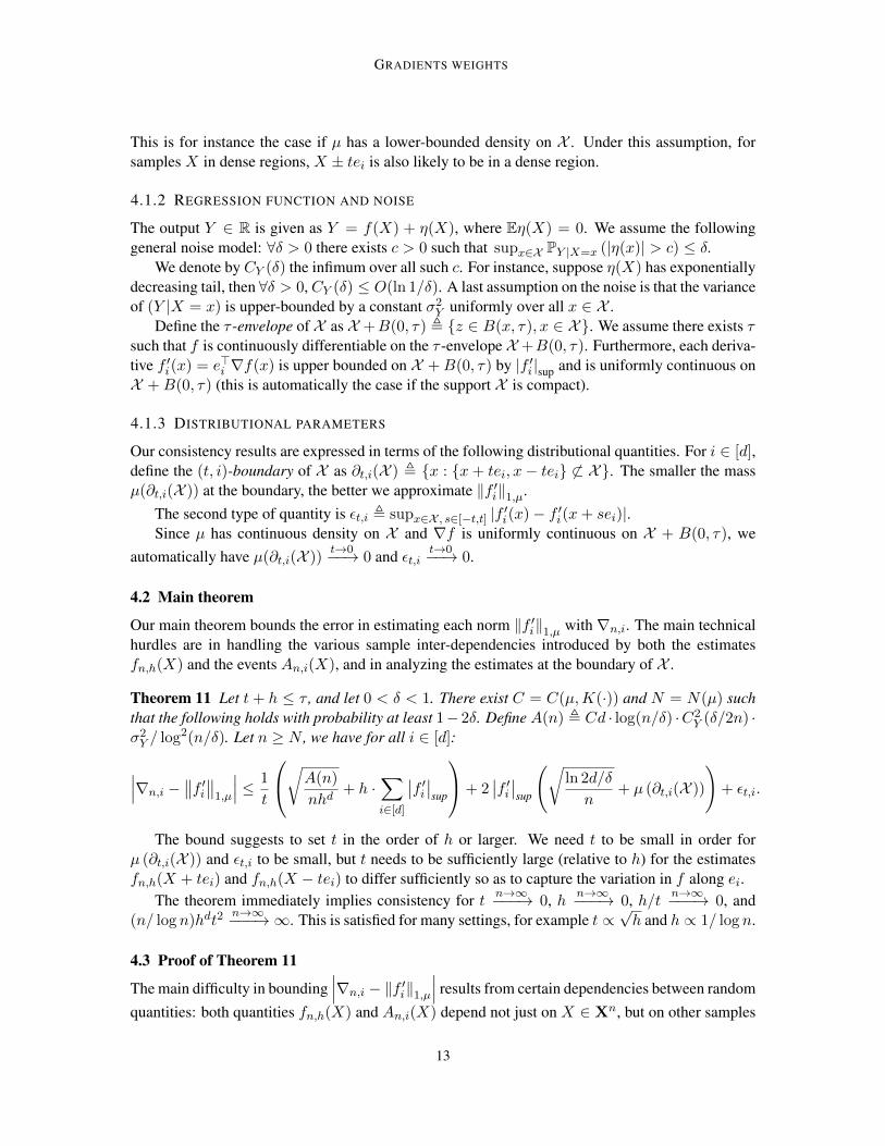
The bound suggests to set t in the order of h or larger. We need t to be small in order forµ (∂t,i(X )) and εt,i to be small, but t needs to be sufficiently large (relative to h) for the estimatesfn,h(X + tei) and fn,h(X − tei) to differ sufficiently so as to capture the variation in f along ei.

The theorem immediately implies consistency for t n→∞−−−→ 0, h n→∞−−−→ 0, h/t n→∞−−−→ 0, and(n/ log n)hdt2

n→∞−−−→∞. This is satisfied for many settings, for example t ∝√h and h ∝ 1/ log n.

4.3 Proof of Theorem 11

The main difficulty in bounding∣∣∣∇n,i − ‖f ′i‖1,µ∣∣∣ results from certain dependencies between random

quantities: both quantities fn,h(X) and An,i(X) depend not just on X ∈ Xn, but on other samples

13


in Xn, and thus introduce inter-dependencies between the estimates ∆t,ifn,h(X) for different pointsX in the sample Xn.

To handle these dependencies, we carefully decompose∣∣∣∇n,i − ‖f ′i‖1,µ∣∣∣, i ∈ [d], starting with:∣∣∣∇n,i − ∥∥f ′i∥∥1,µ

∣∣∣ ≤ ∣∣∇n,i − En∣∣f ′i(X)

∣∣∣∣+∣∣∣En ∣∣f ′i(X)

∣∣− ∥∥f ′i∥∥1,µ

∣∣∣ . (5)

The following simple lemma bounds the second term of (5).

Lemma 12 With probability at least 1− δ, we have for all i ∈ [d],

∣∣∣En ∣∣f ′i(X)∣∣− ∥∥f ′i∥∥1,µ

∣∣∣ ≤ ∣∣f ′i∣∣sup ·√

ln 2d/δ

n.

Proof Apply a Chernoff bound, and a union bound on i ∈ [d].

Now the first term of equation (5) can be further bounded as∣∣∇n,i − En∣∣f ′i(X)

∣∣∣∣ ≤ ∣∣∇n,i − En∣∣f ′i(X)

∣∣ · 1An,i(X)∣∣+ En

∣∣f ′i(X)∣∣ · 1An,i(X)

≤∣∣∇n,i − En

∣∣f ′i(X)∣∣ · 1An,i(X)

∣∣+∣∣f ′i∣∣sup · En1

An,i(X)

. (6)

We will bound each term of (6) separately.The next lemma bounds the second term of (6). It is proved in the appendix. The main tech-

nicality in this lemma is that, for any X in the sample Xn, the event An,i(X) depends on othersamples in Xn.

Lemma 13 Let ∂t,i(X ) be defined as in Section (4.1.3). For n ≥ n(µ), with probability at least1− 2δ, we have for all i ∈ [d],

En1An,i(X)

≤√

ln 2d/δ

n+ µ (∂t,i(X )) .

It remains to bound |∇n,i − En |f ′i(X)| · 1An,i(X)|. To this end we need to bring in fthrough the following quantities:

∇n,i , En[|f(X + tei)− f(X − tei)|

2t· 1An,i(X)

]= En [∆t,if(X) · 1An,i(X)]

and for any x ∈ X , define fn,h(x) , EYn|Xnfn,h(x) =∑

iwi(x)f(xi).The quantity ∇n,i is easily related to En |f ′i(X)|·1An,i(X). This is done in Lemma 14 below.

The quantity fn,h(x) is needed when relating∇n,i to ∇n,i.

Lemma 14 Define εt,i as in Section (4.1.3). With probability at least 1− δ, we have for all i ∈ [d],∣∣∣∇n,i − En∣∣f ′i(X)

∣∣ · 1An,i(X)∣∣∣ ≤ εt,i.

14

GRADIENTS WEIGHTS

Proof We have f(x+ tei)− f(x− tei) =∫ t−t f

′i(x+ sei) ds and therefore

2t(f ′i(x)− εt,i

)≤ f(x+ tei)− f(x− tei) ≤ 2t

(f ′i(x) + εt,i

).

It follows that∣∣ 1

2t |f(x+ tei)− f(x− tei)| − |f ′i(x)|∣∣ ≤ εt,i, therefore∣∣∣∇n,i − En

∣∣f ′i(X)∣∣ · 1An,i(X)

∣∣∣ ≤ En∣∣∣∣ 1

2t|f(x+ tei)− f(x− tei)| −

∣∣f ′i(x)∣∣∣∣∣∣ ≤ εt,i.

It remains to relate Wi to ∇n,i. We have

2t∣∣∣∇n,i − ∇n,i∣∣∣ =2t |En(∆t,ifn,h(X)−∆t,if(X)) · 1An,i(X)|

≤2 maxs∈−t,t

En|fn,h(X + sei)− f(X + sei)| · 1An,i(X)

≤2 maxs∈−t,t

En∣∣∣fn,h(X + sei)− fn,h(X + sei)

∣∣∣ · 1An,i(X) (7)

+ 2 maxs∈−t,t

En∣∣∣fn,h(X + sei)− f(X + sei)

∣∣∣ · 1An,i(X). (8)

We first handle the bias term (8) in the next lemma which is given in the appendix.

Lemma 15 (Bias) Let t+ h ≤ τ . We have for all i ∈ [d], and all s ∈ t,−t:

En∣∣∣fn,h(X + sei)− f(X + sei)

∣∣∣ · 1An,i(X) ≤ h ·∑i∈[d]

∣∣f ′i∣∣sup .

The variance term in (7) is handled in the lemma below. The proof is given in the appendix.

Lemma 16 (Variance terms) There exist C = C(µ,K(·)) such that, with probability at least 1−2δ, we have for all i ∈ [d], and all s ∈ −t, t:

En∣∣∣fn,h(X + sei)− fn,h(X + sei)

∣∣∣ · 1An,i(X) ≤

√Cd · log(n/δ)C2

Y (δ/2n) · σ2Y

n(h/2)d.

The next lemma summarizes the above results:

Lemma 17 Let t+ h ≤ τ and let 0 < δ < 1. There exist C = C(µ,K(·)) such that the followingholds with probability at least 1− 2δ. Define A(n) , Cd · log(n/δ) · C2

Y (δ/2n) · σ2Y / log2(n/δ).

We have

∣∣∇n,i − En∣∣f ′i(X)

∣∣ · 1An,i(X)∣∣ ≤1

t

√A(n)

nhd+ h ·

∑i∈[d]

∣∣f ′i∣∣sup

+ εt,i.

Proof Apply lemmas 14, 15 and 16, in combination with equations 7 and 8.

To complete the proof of Theorem 11, apply lemmas 17 and 12 in combination with equations5 and 6.

15


5. Experimental Evaluation of the GW Approach

We have so far derived GW based on the theoretical principles of Section 2, namely that perfor-mance improvements are possible if data coordinates are weighted according to the coordinate-wisevariation of the unknown f , and if f varies unevenly across coordinates. In this section, we verifythese theoretical principles empirically on various real-world datasets. The code and all the datasets used in these experiments are publicly available at http://goo.gl/bCfS78

We consider kernel, k-NN and SVM (support vector) approaches on a variety of controlled (ar-tificial) and real-world datasets. We emphasize that our goal is to demonstrate the benefits of GW inimproving the performance of these successful and popular procedures on a wide range of datasets.We do not aim to beat results that may have been obtained on these data using procedures otherthan kernel, k-NN and SVM approaches, since this is not required for a practical validation of ourtheoretical results. We also note that, throughout the experiments, we only retain the numerical at-tributes in each data set, and discard all the categorical attributes. Therefore, our reported predictionerrors on some datasets might differ from others reported in the literature at large.

Parameter settings and general comments: Recall that, for the GW approach, we might setthe components Wi of the metric ρ to ∇qn,i. The exponent q (cf. Remark 2.2) is a parameter leftopen by our theoretical analysis. In our experiments, we explore the choices q = 1, as in Kpotufeand Boularias (2012), and q = 2 which serves to further emphasize the difference in importancebetween coordinates.

The resulting performance of the GW approach depends on the parameters used to learn∇n,i ,En [∆t,ifn,h(X) · 1An,i(X)]. These are the bandwidth h used in the estimate fn,h(X) and theparameter t in ∆t,ifn,h(X) , |fn,h(X + tei)− fn,h(X − tei)| /2t. In the majority of experiments(reported in the main body of the paper) we tune h, but we don’t tune t and simply set t = h/2as a rule of thumb. This results in faster training time, and although not optimal, still results insignificant performance gains for the various regression and classification procedures where GW isused to preprocess the data. If in addition we properly tune t, the observed performance gains areeven more significant as reported in Tables 4 and 5 of the Appendix.

We emphasize that the GW approach is computationally cheap: it only adds to training timesince it only involves pre-processing the data. No significant difference is observed in estimationtime, i.e. in computing regression or classification estimates using the preprocessed data vs usingthe original data. In fact estimation time can even be smaller after preprocessing since GW can actas an approximate dimension-reduction given the sparsity in the data. The average prediction timesare reported in Table 6 of the appendix.

Our experiments are divided as follows. First we show the attainable performance gains byusing GW for regression, then we show that GW works well also for classification. At the end ofthe section we explore the tradeoffs between feature selection and feature weigthing.

5.1 Regression experiments

In this section, we present experiments on several real-world regression data sets. We compare theperformances of both kernel regression and k-NN regression in the Euclidean metric space and inthe learned gradient weights metric space.

16

GRADIENTS WEIGHTS

5.1.1 DATA DESCRIPTION

The first two data sets describe the dynamics of 7 degrees of freedom of robotic arms, Barrett WAMand SARCOS (Nguyen-Tuong et al., 2009; Nguyen-Tuong and Peters, 2011). The input points are21-dimensional and correspond to samples of the positions, velocities, and accelerations of the 7joints. The output points correspond to the torque of each joint. The far joints (1, 5, 7) correspondto different regression problems and are the only results reported. As expected, results for otherjoints were found to be similarly good.

Another data set describes the probabilities of achieving successful grasping actions performedby a robot on different piles of objects (Boularias et al., 2014a,b). Each data point describes onegrasping action performed at a particular location on the surface of a pile of objects. The objects aremostly rocks and rubble with unknown and irregular shapes. An input point is a 150-dimensionalvector and corresponds to a patch of a depth image obtained by projecting the robotic hand on thescene. The output is a value between 0 and 1.

The other data sets are taken from the UCI repository (Frank and Asuncion, 2012) and from (Torgo,2012). The concrete strength data set (Concrete Strength) contains 8-dimensional input points, de-scribing age and ingredients of concrete, the output points are the compressive strength. The winequality data set (Wine Quality) contains 11-dimensional input points corresponding to the physico-chemistry of wine samples, the output points are the wine quality. The ailerons data set (Ailerons)is taken from the problem of flying a F16 aircraft. The 5-dimensional input points describe thestatus of the aeroplane, while the goal is to predict the control action on the ailerons of the aircraft.The housing data set (Housing) concerns the task of predicting housing values in areas of Boston,the input points are 13-dimensional. The Parkinson’s Telemonitoring data set (Parkison’s) is usedto predict the clinician’s Parkinson’s disease symptom score using biomedical voice measurementsrepresented by 21-dimensional input points. We also consider a telecommunication problem (Tele-com), wherein the 47-dimensional input points and the output points describe the bandwidth usagein a network.

5.1.2 EXPERIMENTAL SETUP

For all data sets, we normalize each coordinate with its standard deviation from the training data.To learn the metric, we set h by cross-validation on half the training points, and we set t = h/2for all data sets. Note that in practice we might want to also tune t in the range of h for evenbetter performance than reported here. The event An,i(X) is set to reject the gradient estimate∆n,ifn,h(X) at X if no sample contributed to one of the estimates fn,h(X ± tei).

In each experiment, we compare kernel regression in the Euclidean metric space (KR) and inthe learned metric space with gradient weights (KR-ρ) and with squared gradient weights (KR-ρ2),where we use a box kernel for the three methods. Similar comparisons are made using k-NN, k-NN-ρ and k-NN-ρ2. All methods are implemented using a fast neighborhood search procedure, namelythe cover-tree of (Beygelzimer et al., 2006), and we also report in the supplementary material theaverage prediction times so as to confirm that, on average, time-performance is not affected by usingthe metric.

The parameter k in k-NN, k-NN-ρ, k-NN-ρ2, and the bandwidth in KR, KR-ρ, KR-ρ2 arelearned by cross-validation on half of the training points. We try the same range of k (from 1 to5 log n) for the three k-NN methods (k-NN, k-NN-ρ). We try the same range of bandwidth/space-diameter h (a grid of size 0.02 from 1 to 0.02 ) for the three KR methods (KR, KR-ρ, KR-ρ2): this

17


is done efficiently by starting with a log search to quickly reduce the search space, followed by agrid search on the resulting smaller range.

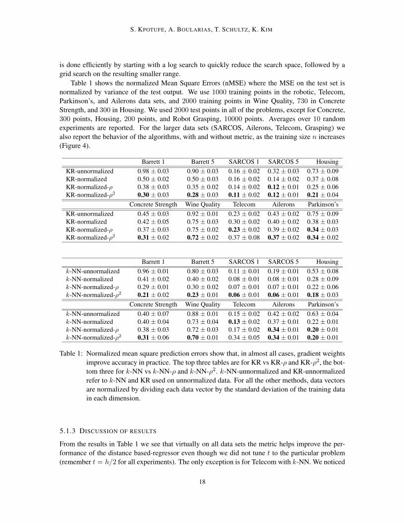
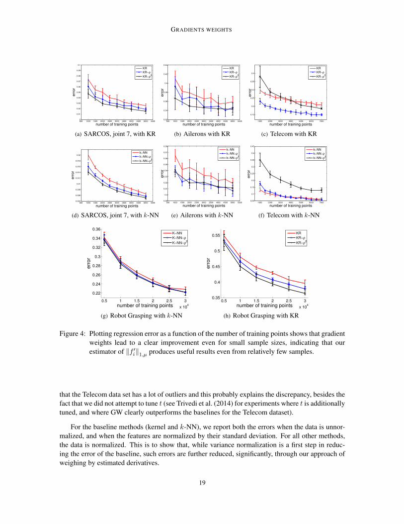
Table 1 shows the normalized Mean Square Errors (nMSE) where the MSE on the test set isnormalized by variance of the test output. We use 1000 training points in the robotic, Telecom,Parkinson’s, and Ailerons data sets, and 2000 training points in Wine Quality, 730 in ConcreteStrength, and 300 in Housing. We used 2000 test points in all of the problems, except for Concrete,300 points, Housing, 200 points, and Robot Grasping, 10000 points. Averages over 10 randomexperiments are reported. For the larger data sets (SARCOS, Ailerons, Telecom, Grasping) wealso report the behavior of the algorithms, with and without metric, as the training size n increases(Figure 4).

Barrett 1 Barrett 5 SARCOS 1 SARCOS 5 HousingKR-unnormalized 0.98 ± 0.03 0.90 ± 0.03 0.16 ± 0.02 0.32 ± 0.03 0.73 ± 0.09KR-normalized 0.50 ± 0.02 0.50 ± 0.03 0.16 ± 0.02 0.14 ± 0.02 0.37 ± 0.08KR-normalized-ρ 0.38 ± 0.03 0.35 ± 0.02 0.14 ± 0.02 0.12 ± 0.01 0.25 ± 0.06KR-normalized-ρ2 0.30 ± 0.03 0.28 ± 0.03 0.11 ± 0.02 0.12 ± 0.01 0.21 ± 0.04

Concrete Strength Wine Quality Telecom Ailerons Parkinson’sKR-unnormalized 0.45 ± 0.03 0.92 ± 0.01 0.23 ± 0.02 0.43 ± 0.02 0.75 ± 0.09KR-normalized 0.42 ± 0.05 0.75 ± 0.03 0.30 ± 0.02 0.40 ± 0.02 0.38 ± 0.03KR-normalized-ρ 0.37 ± 0.03 0.75 ± 0.02 0.23 ± 0.02 0.39 ± 0.02 0.34 ± 0.03KR-normalized-ρ2 0.31 ± 0.02 0.72 ± 0.02 0.37 ± 0.08 0.37 ± 0.02 0.34 ± 0.02

Barrett 1 Barrett 5 SARCOS 1 SARCOS 5 Housingk-NN-unnormalized 0.96 ± 0.01 0.80 ± 0.03 0.11 ± 0.01 0.19 ± 0.01 0.53 ± 0.08k-NN-normalized 0.41 ± 0.02 0.40 ± 0.02 0.08 ± 0.01 0.08 ± 0.01 0.28 ± 0.09k-NN-normalized-ρ 0.29 ± 0.01 0.30 ± 0.02 0.07 ± 0.01 0.07 ± 0.01 0.22 ± 0.06k-NN-normalized-ρ2 0.21 ± 0.02 0.23 ± 0.01 0.06 ± 0.01 0.06 ± 0.01 0.18 ± 0.03

Concrete Strength Wine Quality Telecom Ailerons Parkinson’sk-NN-unnormalized 0.40 ± 0.07 0.88 ± 0.01 0.15 ± 0.02 0.42 ± 0.02 0.63 ± 0.04k-NN-normalized 0.40 ± 0.04 0.73 ± 0.04 0.13 ± 0.02 0.37 ± 0.01 0.22 ± 0.01k-NN-normalized-ρ 0.38 ± 0.03 0.72 ± 0.03 0.17 ± 0.02 0.34 ± 0.01 0.20 ± 0.01k-NN-normalized-ρ2 0.31 ± 0.06 0.70 ± 0.01 0.34 ± 0.05 0.34 ± 0.01 0.20 ± 0.01

Table 1: Normalized mean square prediction errors show that, in almost all cases, gradient weightsimprove accuracy in practice. The top three tables are for KR vs KR-ρ and KR-ρ2, the bot-tom three for k-NN vs k-NN-ρ and k-NN-ρ2. k-NN-unnormalized and KR-unnormalizedrefer to k-NN and KR used on unnormalized data. For all the other methods, data vectorsare normalized by dividing each data vector by the standard deviation of the training datain each dimension.

5.1.3 DISCUSSION OF RESULTS

From the results in Table 1 we see that virtually on all data sets the metric helps improve the per-formance of the distance based-regressor even though we did not tune t to the particular problem(remember t = h/2 for all experiments). The only exception is for Telecom with k-NN. We noticed

18

GRADIENTS WEIGHTS

500 1000 1500 2000 2500 3000 3500 4000 4500 5000 55000

0.01

0.02

0.03

0.04

0.05

0.06

0.07

0.08

0.09

0.1

number of training points

err

or

KR

KR−ρ

KR−ρ2

(a) SARCOS, joint 7, with KR

500 1000 1500 2000 2500 3000 3500 4000 4500 5000 55000.32

0.34

0.36

0.38

0.4

0.42

0.44


err

or

KR

KR−ρ

KR−ρ2

(b) Ailerons with KR

1000 2000 3000 4000 5000 6000 7000

0.15

0.2

0.25

0.3

0.35

0.4


err

or

KR

KR−ρ

KR−ρ2

(c) Telecom with KR

500 1000 1500 2000 2500 3000 3500 4000 4500 5000 55000.004

0.006

0.008

0.01

0.012

0.014

0.016

0.018

0.02


err

or

k−NN

k−NN−ρ

k−NN−ρ2

(d) SARCOS, joint 7, with k-NN

500 1000 1500 2000 2500 3000 3500 4000 4500 5000 55000.29

0.3

0.31

0.32

0.33

0.34

0.35

0.36

0.37

0.38


err

or

k−NN

k−NN−ρ

k−NN−ρ2

(e) Ailerons with k-NN

1000 2000 3000 4000 5000 6000 70000.05

0.1

0.15

0.2

0.25

0.3

0.35

0.4

0.45


err

or

k−NN

k−NN−ρ

k−NN−ρ2

(f) Telecom with k-NN

0.5 1 1.5 2 2.5 3

x 104

0.22

0.24

0.26

0.28

0.3

0.32

0.34

0.36


err

or

K−NN

K−NN−ρ

K−NN−ρ2

(g) Robot Grasping with k-NN

0.5 1 1.5 2 2.5 3

x 104

0.35

0.4

0.45

0.5

0.55


err

or

KR

KR−ρ

KR−ρ2

(h) Robot Grasping with KR

Figure 4: Plotting regression error as a function of the number of training points shows that gradientweights lead to a clear improvement even for small sample sizes, indicating that ourestimator of ‖f ′i‖1,µ produces useful results even from relatively few samples.

that the Telecom data set has a lot of outliers and this probably explains the discrepancy, besides thefact that we did not attempt to tune t (see Trivedi et al. (2014) for experiments where t is additionallytuned, and where GW clearly outperforms the baselines for the Telecom dataset).

For the baseline methods (kernel and k-NN), we report both the errors when the data is unnor-malized, and when the features are normalized by their standard deviation. For all other methods,the data is normalized. This is to show that, while variance normalization is a first step in reduc-ing the error of the baseline, such errors are further reduced, significantly, through our approach ofweighing by estimated derivatives.

19


Also notice that the error of k-NN is already low for small sample sizes, making it harder tooutperform. However, as shown in Figure 4, for larger training sizes k-NN-ρ gains on k-NN. Wealso note that methods using squared gradient weights (k-NN-ρ2 and KR-ρ2) achieved a betterperformance compared to other methods. The only exception here is also Telecom, where the non-squared gradient weights yield a lower prediction error. The rest of the results in Figure 4 where wevary n are self-descriptive: gradient weighting clearly improves the performance of the distance-based regressors.

Finally, we note that the average prediction times (reported in the supplementary material) isnearly the same for all the methods. Last, remember that the metric can be learned online at the costof only 2d times the average kernel estimation time reported.

5.2 Classification experiments

5.2.1 DATA DESCRIPTION

We tested the gradient weights method on six different data sets taken from the UCI repository (Frankand Asuncion, 2012) and from the LIBSVM website (Fan, 2012). The covertype data set containspredictions of binary forest cover types from cartographic features given by 10 real variables among54 other variables. This data set originally consists of seven different cover types, but only the twolargest categories are selected for binary classification. The MAGIC gamma data set consists of 10features and predicts the registration of high energy gamma particles in a ground-based atmosphericCherenkov gamma telescope. The IJCNN data set contains predictions of one binary output fromfour different time series, described by 10 categorical variables and 12 real variables. The shuttledata set contains 9 numerical attributes. The original data set has seven different categories, butfor binary classification we merged all the classes into one class, except the first class which corre-sponds to approximately 80% of all the data. The page blocks data set predicts whether a blockin a given document is a text block using 10 real-valued features. We also consider the thyroiddata set where the problem is to determine whether a given patient is hypothyroid. There are threedifferent output classes in this data set, the condition of a patient is described by 6 real variables and15 categorical variables.

5.2.2 EXPERIMENTAL SETUP

The setup for the classification experiments is similar to the one used in the regression experiments.For all data sets, we normalize each coordinate with its standard deviation from the training data.We use the training data to compute the gradient weights. Parameter t is set proportionally tothe difference between the minimum and the maximum values of each feature to account for thedifferences between features scales that remain after normalization. One can also consider usingthe learned gradient weights to set t and to re-estimate the gradient weights again, in a repeatediterative process. The probability P (Ci|x) of each classCi, used for calculating the feature weights,is estimated by weighted k-NN with Gaussian kernel.

In each experiment, we compare a k nearest neighbor classifier in the Euclidean metric space(k-NN), the learned metric space with gradient weights (k-NN-ρ), and a metric space in which gra-dient weights have been squared (k-NN-ρ2). Analogous results have been obtained using an ε-NNclassifier (ε-NN, ε-NN-ρ, ε-NN-ρ2) which uses all training samples within an ε-ball around the testpoint, rather than the k nearest neighbors. Parameters k and ε have been set by cross-validation withhalf the training points. As in the regression experiments, k and ε are found by using a log search,

20

GRADIENTS WEIGHTS

0 500 1000 1500 2000 2500 3000 35000.22

0.24

0.26

0.28

0.3

0.32

0.34

0.36


err

or

k−NN

k−NN−ρ

k−NN−ρ2

(a) Covertype with k-NN

0 500 1000 1500 2000 2500 3000 35000.03

0.04

0.05

0.06

0.07

0.08

0.09


err

or

k−NN

k−NN−ρ

k−NN−ρ2

(b) IJCNN with k-NN

500 1000 1500 2000 2500 3000 3500

0.04

0.045

0.05

0.055

0.06

0.065

0.07


err

or

k−NN

k−NN−ρ

k−NN−ρ2

(c) Thyroid with k-NN

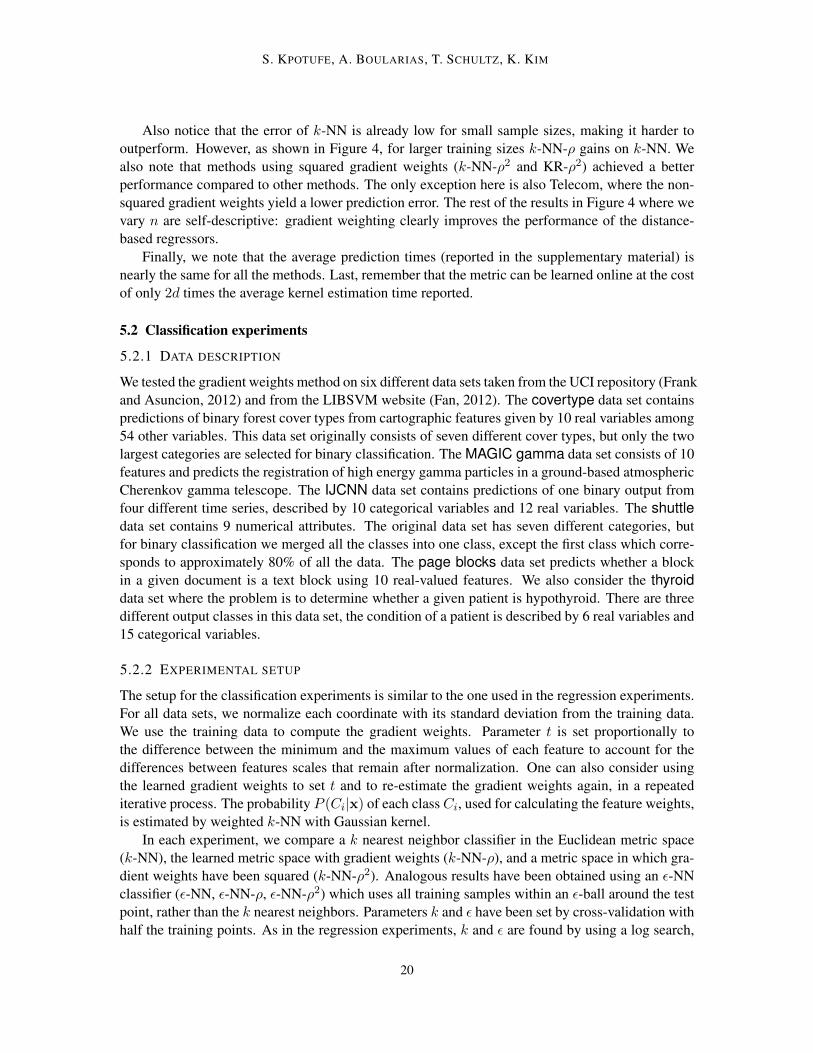
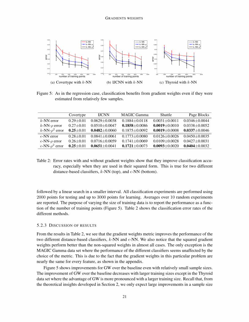
Figure 5: As in the regression case, classification benefits from gradient weights even if they wereestimated from relatively few samples.

Covertype IJCNN MAGIC Gamma Shuttle Page Blocksk-NN error 0.29±0.01 0.0629±0.0038 0.1884±0.0118 0.0031±0.0011 0.0346±0.0044k-NN-ρ error 0.27±0.01 0.0510±0.0047 0.1858±0.0086 0.0019±0.0010 0.0338±0.0052k-NN-ρ2 error 0.25±0.01 0.0482±0.0060 0.1875±0.0092 0.0019±0.0008 0.0337±0.0046e-NN error 0.28±0.01 0.0841±0.0061 0.1773±0.0080 0.0126±0.0026 0.0450±0.0035e-NN-ρ error 0.26±0.01 0.0716±0.0059 0.1741±0.0069 0.0109±0.0028 0.0427±0.0031e-NN-ρ2 error 0.25±0.01 0.0651±0.0041 0.1721±0.0073 0.0093±0.0020 0.0404±0.0032

Table 2: Error rates with and without gradient weights show that they improve classification accu-racy, especially when they are used in their squared form. This is true for two differentdistance-based classifiers, k-NN (top), and ε-NN (bottom).

followed by a linear search in a smaller interval. All classification experiments are performed using2000 points for testing and up to 3000 points for learning. Averages over 10 random experimentsare reported. The purpose of varying the size of training data is to report the performance as a func-tion of the number of training points (Figure 5). Table 2 shows the classification error rates of thedifferent methods.

5.2.3 DISCUSSION OF RESULTS

From the results in Table 2, we see that the gradient weights metric improves the performance of thetwo different distance-based classifiers, k-NN and ε-NN. We also notice that the squared gradientweights perform better than the non-squared weights in almost all cases. The only exception is theMAGIC Gamma data set where the performance of the different classifiers seems unaffected by thechoice of the metric. This is due to the fact that the gradient weights in this particular problem arenearly the same for every feature, as shown in the appendix.

Figure 5 shows improvements for GW over the baseline even with relatively small sample sizes.The improvement of GW over the baseline decreases with larger training sizes except in the Thyroiddata set where the advantage of GW is more pronounced with a larger training size. Recall that, fromthe theoretical insights developed in Section 2, we only expect large improvements in a sample size

21


0 2 4 6 8 10 12 14 16 18 20 220

0.1

0.2

0.3

0.4

0.5

0.6

0.7

0.8

number of selected features

err

or

KR with feature selection

KR−ρ

KR−ρ2

(a) Barrett, joint 1

0 2 4 6 8 10 12 14 16 18 20 220

0.1

0.2

0.3

0.4

0.5

0.6

0.7

0.8


err

or


KR−ρ

KR−ρ2

(b) Barrett, joint 5

0 2 4 6 8 10 12 14 16 18 20 220.1

0.15

0.2

0.25

0.3

0.35

0.4


err

or


KR−ρ

KR−ρ2

(c) Sarcos, joint 1

0 2 4 6 8 10 12 14 16 18 20 220.1

0.15

0.2

0.25

0.3

0.35

0.4

0.45

0.5

0.55

0.6


err

or


KR−ρ

KR−ρ2

(d) Sarcos, joint 5

0 2 4 6 8 10 12 140.1

0.2

0.3

0.4

0.5

0.6

0.7

0.8


err

or


KR−ρ

KR−ρ2

(e) Housing

0 1 2 3 4 5 6 7 8 9

0.3

0.4

0.5

0.6

0.7

0.8

0.9


err

or


KR−ρ

KR−ρ2

(f) Concrete Strength

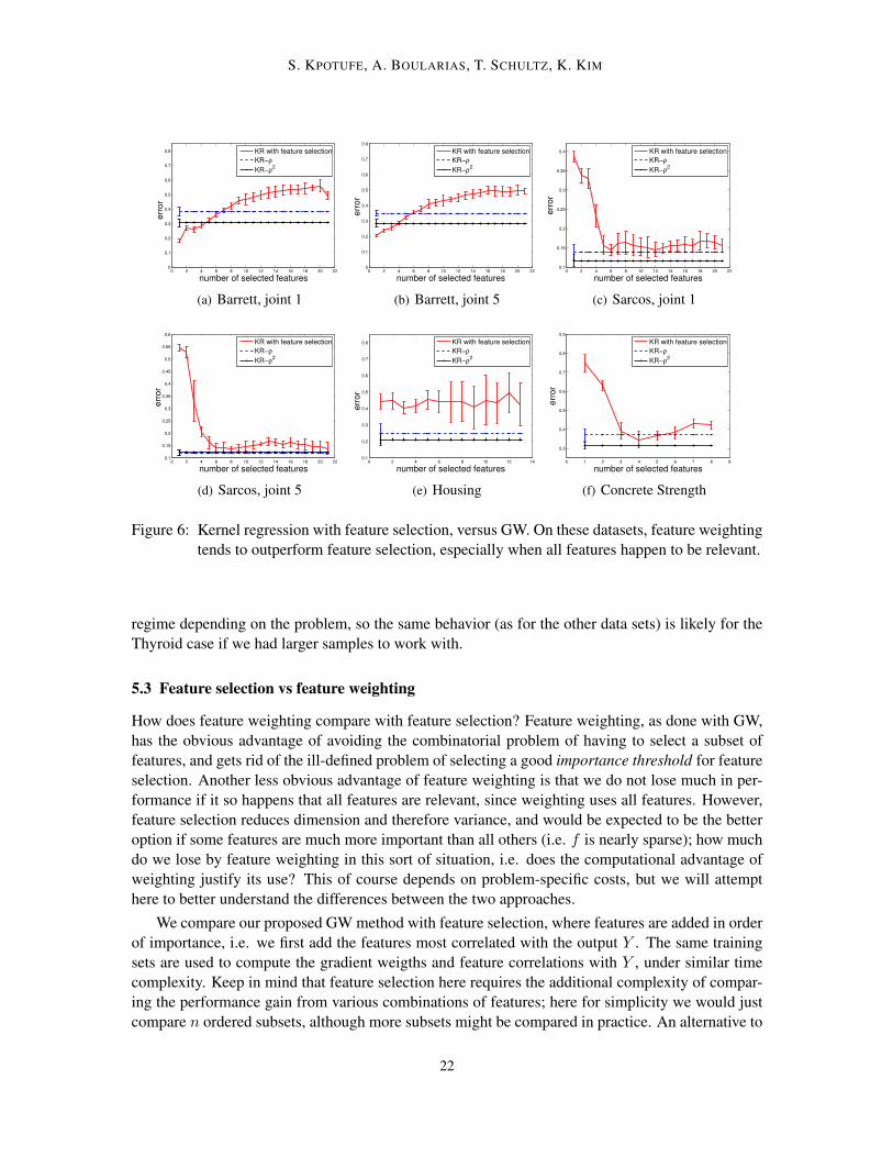
Figure 6: Kernel regression with feature selection, versus GW. On these datasets, feature weightingtends to outperform feature selection, especially when all features happen to be relevant.

regime depending on the problem, so the same behavior (as for the other data sets) is likely for theThyroid case if we had larger samples to work with.

5.3 Feature selection vs feature weighting

How does feature weighting compare with feature selection? Feature weighting, as done with GW,has the obvious advantage of avoiding the combinatorial problem of having to select a subset offeatures, and gets rid of the ill-defined problem of selecting a good importance threshold for featureselection. Another less obvious advantage of feature weighting is that we do not lose much in per-formance if it so happens that all features are relevant, since weighting uses all features. However,feature selection reduces dimension and therefore variance, and would be expected to be the betteroption if some features are much more important than all others (i.e. f is nearly sparse); how muchdo we lose by feature weighting in this sort of situation, i.e. does the computational advantage ofweighting justify its use? This of course depends on problem-specific costs, but we will attempthere to better understand the differences between the two approaches.

We compare our proposed GW method with feature selection, where features are added in orderof importance, i.e. we first add the features most correlated with the output Y . The same trainingsets are used to compute the gradient weigths and feature correlations with Y , under similar timecomplexity. Keep in mind that feature selection here requires the additional complexity of compar-ing the performance gain from various combinations of features; here for simplicity we would justcompare n ordered subsets, although more subsets might be compared in practice. An alternative to

22

GRADIENTS WEIGHTS

0 2 4 6 8 10 120.2

0.25

0.3

0.35

0.4

0.45

0.5


Err

or

k−NN with feature selection

k−NN−ρ

k−NN−ρ2

(a) Covertype

0 2 4 6 8 10 12 140.04

0.05

0.06

0.07

0.08

0.09

0.1

0.11


Err

or


k−NN−ρ

k−NN−ρ2

(b) IJCNN

0 2 4 6 8 10 120.16

0.18

0.2

0.22

0.24

0.26

0.28

0.3


Err

or


k−NN−ρ

k−NN−ρ2

(c) MAGIC Gamma

0 1 2 3 4 5 6 7 8 9 100

0.02

0.04

0.06

0.08

0.1

0.12

0.14


Err

or


k−NN−ρ

k−NN−ρ2

(d) Shuttle

0 2 4 6 8 10 120.02

0.03

0.04

0.05

0.06

0.07

0.08


Err

or


k−NN−ρ

k−NN−ρ2

(e) Page Blocks

0 1 2 3 4 5 6 70.025

0.03

0.035

0.04

0.045

0.05

0.055

0.06

0.065

0.07


Err

or


k−NN−ρ

k−NN−ρ2

(f) Thyroid

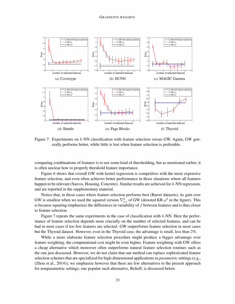
Figure 7: Experiments on k-NN classification with feature selection versus GW. Again, GW gen-erally performs better, while little is lost when feature selection is preferable.

comparing combinations of features is to use some kind of thresholding, but as mentioned earlier, itis often unclear how to properly threshold feature importance.

Figure 6 shows that overall GW with kernel regression is competitive with the more expensivefeature selection, and even often achieves better performance in those situations where all featureshappen to be relevant (Sarcos, Housing, Concrete). Similar results are achieved for k-NN regression,and are reported in the supplementary material.

Notice that, in those cases where feature selection performs best (Barret datasets), its gain overGW is smallest when we used the squared version ∇2

n,i of GW (denoted KR-ρ2 in the figure). Thisis because squaring emphasizes the differences in variability of f between features and is thus closerto feature selection.

Figure 7 repeats the same experiments in the case of classification with k-NN. Here the perfor-mance of feature selection depends more crucially on the number of selected features, and can bebad in most cases if too few features are selected. GW outperforms feature selection in most casesbut the Thyroid dataset. However, even in the Thyroid case, the advantage is small, less than 2%.

While a more elaborate feature selection procedure might produce a bigger advantage overfeature weighting, the computational cost might be even higher. Feature weighting with GW offersa cheap alternative which moreover often outperforms natural feature selection routines such asthe one just discussed. However, we do not claim that our method can replace sophisticated featureselection schemes that are specialized for high-dimensional applications in parametric settings (e.g.,(Zhou et al., 2014)); we emphasize however that there are few alternatives to the present approachfor nonparametric settings; one popular such alternative, Relieff, is discussed below.

23


0 500 1000 1500 2000 2500 3000 35000.22

0.24

0.26

0.28

0.3

0.32

0.34


err

or

SVM

SVM−ρ

SVM−ρ2

(a) Covertype with SVM

0 500 1000 1500 2000 2500 3000 35000.04

0.05

0.06

0.07

0.08

0.09

0.1


err

or

SVM

SVM−ρ

SVM−ρ2

(b) IJCNN with SVM

500 1000 1500 2000 2500 3000 3500

0.04

0.045

0.05

0.055

0.06

0.065

0.07

0.075

0.08


err

or

SVM

SVM−ρ

SVM−ρ2

(c) Thyroid with SVM

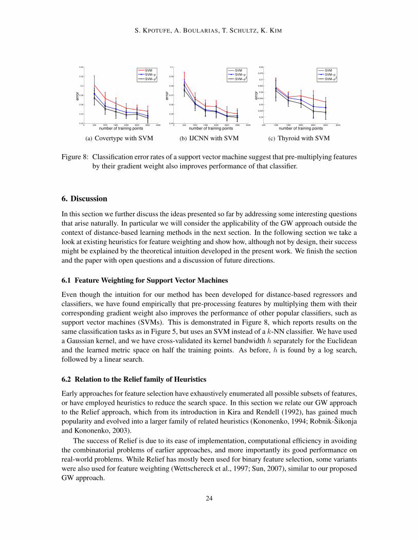
Figure 8: Classification error rates of a support vector machine suggest that pre-multiplying featuresby their gradient weight also improves performance of that classifier.

6. Discussion

In this section we further discuss the ideas presented so far by addressing some interesting questionsthat arise naturally. In particular we will consider the applicability of the GW approach outside thecontext of distance-based learning methods in the next section. In the following section we take alook at existing heuristics for feature weighting and show how, although not by design, their successmight be explained by the theoretical intuition developed in the present work. We finish the sectionand the paper with open questions and a discussion of future directions.

6.1 Feature Weighting for Support Vector Machines

Even though the intuition for our method has been developed for distance-based regressors andclassifiers, we have found empirically that pre-processing features by multiplying them with theircorresponding gradient weight also improves the performance of other popular classifiers, such assupport vector machines (SVMs). This is demonstrated in Figure 8, which reports results on thesame classification tasks as in Figure 5, but uses an SVM instead of a k-NN classifier. We have useda Gaussian kernel, and we have cross-validated its kernel bandwidth h separately for the Euclideanand the learned metric space on half the training points. As before, h is found by a log search,followed by a linear search.

6.2 Relation to the Relief family of Heuristics

Early approaches for feature selection have exhaustively enumerated all possible subsets of features,or have employed heuristics to reduce the search space. In this section we relate our GW approachto the Relief approach, which from its introduction in Kira and Rendell (1992), has gained muchpopularity and evolved into a larger family of related heuristics (Kononenko, 1994; Robnik-Sikonjaand Kononenko, 2003).

The success of Relief is due to its ease of implementation, computational efficiency in avoidingthe combinatorial problems of earlier approaches, and more importantly its good performance onreal-world problems. While Relief has mostly been used for binary feature selection, some variantswere also used for feature weighting (Wettschereck et al., 1997; Sun, 2007), similar to our proposedGW approach.

24

GRADIENTS WEIGHTS

Covertype MAGIC Gamma Shuttle Page BlocksGradient Weights 0.0113±0.0067 0.0050±0.0039 0.0006±0.0011 0.0007±0.0026ReliefF 0.0229±0.0075 0.0147±0.0072 -0.0019±0.0024 -0.0019±0.0049

Table 3: Comparing the improvement in classification error over the k-NN baseline when usingsquared gradient weights or ReliefF shows that none of the two methods dominates theother one. Negative numbers indicate cases where ReliefF led to increased errors.

While Relief and our GW approach have similar practical benefits, GW is grounded in the the-oretical insights developed earlier in this work. Corollary 8 allows us to theoretically understandthe conditions under which GW improves regression rates in a minimax sense, opening up potentialdirections for further development of feature weighting methods. To the best of our knowledge, nosuch theoretical results are available for Relief although various works have provided theoreticalinterpretation (e.g. (Sun, 2007)) without actually analyzing the direct effect of Relief weights onregression or classification convergence rates. We will argue here that the theoretical intuition de-veloped in this work helps explain some of the success of Relief: the weights computed by Relief,similar to those of GW, are generally correlated with the coordinate-wise variation of the unknownregression function f .

(a) Covertype (b) MAGIC Gamma (c) Page Blocks (d) Shuttle

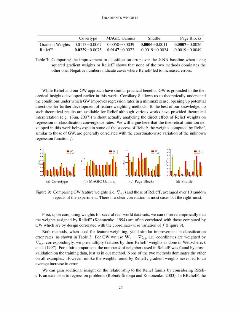
Figure 9: Comparing GW feature weights (i.e. ∇n,i) and those of ReliefF, averaged over 10 randomrepeats of the experiment. There is a clear correlation in most cases but the right-most.

First, upon computing weights for several real-world data sets, we can observe empirically thatthe weights assigned by ReliefF (Kononenko, 1994) are often correlated with those computed byGW which are by design correlated with the coordinate-wise variation of f (Figure 9).

Both methods, when used for feature-weighting, yield similar improvement in classificationerror rates, as shown in Table 3. For GW we use Wi = ∇2

n,i, i.e. coordinates are weighted by∇n,i; correspondingly, we pre-multiply features by their ReliefF weights as done in Wettscherecket al. (1997). For a fair comparison, the number k of neighbors used in ReliefF was found by cross-validation on the training data, just as in our method. None of the two methods dominates the otheron all examples. However, unlike the weights found by ReliefF, gradient weights never led to anaverage increase in error.

We can gain additional insight on the relationship to the Relief family by considering RReli-efF, an extension to regression problems (Robnik-Sikonja and Kononenko, 2003). In RReliefF, the

25


weight Wi of a feature i is estimated as

Wi =

∑x

∑x′∈N(x) |fn(x)− fn(x′)||xi − x′i|dis(x, x′)∑x

∑x′∈N(x) |fn(x)− fn(x′)|dis(x, x′)

−

∑x

∑x′∈N(x)

(|xi − x′i|dis(x, x′)− |fn(x)− fn(x′)||xi − x′i|dis(x, x′)

)n−

∑x

∑x′∈N(x) |fn(x)− fn(x′)|dis(x, x′)

,

where x is a training input point, xi is the ith attribute of x, n is the number of training points, fnis a k-NN estimate of f , N(x) is the set of k nearest neighbors of x with respect to the Euclideanmetric, and dis is a dissimilarity function, defined as dis(x, x′) = exp

(− 1

h

(rank(x, x′)

)2) where

rank(x, x′) is obtained by ranking the neighbors of x according to their increasing distance from x,and h is some bandwidth. By rearranging the terms of the equation above, we have

Wi =

(1

A(fn)+

1

B(fn)

)∑x

∑x′∈N(x)

|fn(x)− fn(x′)||xi − x′i|dis(x, x′)

− 1

B(fn)

∑x

∑x′∈N(x)

|xi − x′i|dis(x, x′)

=

(1

A(fn)+

1

B(fn)

)Wi,I +

1

B(fn)Wi,II ,

where

A(fn) =∑

x

∑x′∈N(x) |fn(x)− fn(x′)|dis(x, x′),

B(fn) = n−∑

x

∑x′∈N(x) |fn(x)− fn(x′)|dis(x, x′).

Notice thatA(fn) andB(fn) are global parameters that do not depend on the feature i for whichthe weight Wi is calculated.

The term 1B(fn)Wi,II can be interpreted as a measure of the spread of the input points around

axis i, and has little dependence on the output Y . Moreover this term would generally be negligible:suppose w.l.o.g. that |Y | is normalized to be at most 1, then B(fn) = Ω(n) so the term goes to 0.

The other term(

1A(fn) + 1

B(fn)

)Wi,I is most important and is correlated with the variation of

fn (hence of f ) in direction i. In particular, Wi,I has the essential ingredients of an estimator of‖f ′i‖1,µ: it is a weighted average of differences in fn, where the weights (|xi − x′i|dis(x, x′)) are(1) larger for pairs of points aligned along coordinate i (via |xi − x′i|), and (2) larger for the closestpairs of points (via the dissimilarity dis(x, x′)).

In fact the differences between Wi,I and our estimator ∇n,i are simply in the way we accom-plish (1) and (2) above: we directly look at pairs of points (x ± tei), t-close and aligned with thecoordinate i. This is similar to setting the neighborhood N(x) in Relieff to x ± tei and using adissimilarity of the form dis(x, x′) =

(2nt2

)−1.The success of GW is best understood in terms of how they reduce the variance of distance-

based regressors while controlling bias, as elucidated in Section 2.2. Even though no such analysisis available for Relief, our results extend the same theoretical intuition to the RReliefF heuristicwhich also estimates a quantity that is correlated with the coordinate-wise variation of f .

26

GRADIENTS WEIGHTS

6.3 Final Remarks and Future Directions

We have shown both theoretically and empirically that it is possible to gain significantly in re-gression and classification performance by weighting features according to the way the unknownregression function f varies along coordinates, provided f does not vary equally across coordinates,which is often the case. We derived a simple procedure to estimate the variation in f and showedits consistency. The present brings up many new questions which we hope would be the subject offuture investigation. We list some of these questions below.

The approach results in a two-phase prediction procedure, which however might be iterated intoa multiple phase procedure for a potentially better estimation of f . A natural question is how todetect convergence of a multiple phase approach. This is unclear for now, but is worth pursuingsince even the simple two-phase approach discussed here works well.

The approach presented in this paper weights coordinates with some power of the estimate∇n,i of the gradient norm ‖f ′i‖1,µ. Should all coordinates be weighted with the same power of∇n,i, or is there a better way to weights coordinates according to the way f varies? This questionrequires refined theoretical understanding of how coordinate-weighting affects particular regressionand classification procedures.

The current approach does not take into account the fact that the input X might not be full-dimensional. It is often the case that data lies near lower-dimensional subspaces of Rd. How doesone capture the directional variation of f in these cases?

Given the simplicity and success of the approach presented here, we believe even better feature-weigthing approaches are lurking close, and some of the above questions are potential directions forfurther improvement.

Acknowledgments

A significant part of this work was conducted when the authors were at the Max Planck Institute forIntelligent Systems, Tuebingen, Germany.

Appendix A. Consistency lemmas

We need the following VC result.

Lemma 18 (Relative VC bounds (Vapnik and Chervonenkis, 1971)) Let 0 < δ < 1 and defineαn = (2d ln 2n+ ln(4/δ)) /n.

Then with probability at least 1− δ over the choice of Xn, all balls B ∈ Rd satisfy

µ(B) ≤ µn(B) +√µn(B)αn + αn.

Proof [Lemma 13] Let Ai(X) denote the event that mins∈−t,t µ(B(X + sei, h/2)) < 3αn. ByLemma 18, with probability at least 1−δ, ∀i ∈ [d], An,i(X) =⇒ Ai(X) so that En1

An,i(X)

≤

En1Ai(X)

.

Using a Chernoff bound, followed by a union bound on [d], we also have with probability atleast 1− δ that En1

Ai(X)

≤ E1

Ai(X)

+√

ln(2d/δ)/n.Finally, E1

Ai(X)

≤ E

[1Ai(X)

|X ∈ X \ ∂t,i(X )

]+ µ (∂t,i(X )). The first term is 0 for

large n. This is true since, for x ∈ X \ ∂t,i(X ), for all i ∈ [d] and s ∈ −t, t, x + sei ∈ X , and

27


therefore µ(B(x+ sei, h/2)) ≥ Cµ(h/2)d ≥ 3αn for our setting of h (see Section 3).

Proof [Lemma 15] Let x = X + sei. For any Xi ∈ Xn, let vi denote the unit vector in direction(Xi − x). We have∣∣∣fn,h(x)− f(x)

∣∣∣ ≤∑i

wi(x) |f(Xi)− f(x)| =∑i

wi(x)

∣∣∣∣∣∫ ‖Xi−x‖

0v>i ∇f(x+ svi) ds

∣∣∣∣∣≤∑i

wi(x) ‖Xi − x‖ · maxx′∈X+B(0,τ)

∥∥∥v>i ∇f(x′)∥∥∥ ≤ h ·∑

i∈[d]

∣∣f ′i∣∣sup .

Multiply the l.h.s. by 1An,i(X), take the empirical expectation and conclude.

The variance (Lemma 16) is handled in a way similar to an analysis of (Kpotufe, 2011) on k-NN regression. The additional technicality in the present result is due to the fact that, unlike in thecase of k-NN, the number of points contributing to the estimate (and hence the variance) is not aconstant.Proof [Lemma 16] Assume that An,i(X) is true, and fix x = X + sei. The following variancebound is quickly obtained:

EYn|Xn

∣∣∣fn,h(x)− fn,h(x)∣∣∣2 ≤ σ2

Y ·∑i∈[n]

wi(x) ≤ σ2Y ·max

i∈[n]wi(x).

Let Ynx denote the Y values of samplesXi ∈ B(x, h), and writeψ(Yn

x) ,∣∣∣fn,h(x)− fn,h(x)

∣∣∣.We next relate ψ(Yn

x) to the above variance.Let Yδ denote the event that for all Yi ∈ Yn, |Yi − f(Xi)| ≤ CY (δ/2n) · σY . By definition of

CY (δ/2n), the event Yδ happens with probability at least 1− δ/2 ≥ 1/2. We therefore have that

PYn|Xn

(ψ(Yn

x) > 2EYn|Xnψ(Ynx) + ε

)≤ PYn|Xn

(ψ(Yn

x) > EYn|Xn,Yδψ(Ynx) + ε

)≤ PYn|Xn,Yδ

(ψ(Yn


)+ δ/2.

Now, it can be verified that, by McDiarmid’s inequality, we have

PYn|Xn,Yδ(ψ(Yn


)≤ exp

−2ε2/C2Y (δ/2n) · σ2

Y

∑i∈[n]

w2i (x)

.

Notice that the number of possible sets Ynx (over x ∈ X ) is at most the n-shattering number of

balls in Rd. By Sauer’s lemma we know this number is bounded by (2n)d+2. We therefore have bya union bound that, with probability at least 1− δ, for all x ∈ X satisfying B(x, h/2) ∩Xn 6= ∅,

ψ(Ynx) ≤ 2EYn|Xnψ(Yn

x) +

√(d+ 2) · log(n/δ)C2

Y (δ/2n) · σ2Y

∑i∈[n]

w2i (x)

≤ 2(EYn|Xnψ2(Yn

x))1/2

+√

(d+ 2) · log(n/δ)C2Y (δ/2n) · σ2

Y ·maxiwi(x)

≤√Cd · log(n/δ)C2

Y (δ/2n) · σ2Y /nµn((B(x, h/2)),

28

GRADIENTS WEIGHTS

where the second inequality is obtained by applying Jensen’s, and the last inequality is due to thefact that the kernel weights are upper and lower-bounded on B(x, h/2).

Now by Lemma 18, with probability at least 1− δ, for all X such that An,i(X) is true, we havefor all s ∈ −t, t, 3µn((B(x, h/2)) ≥ µ((B(x, h/2)) ≥ Cµ(h/2)d. Integrate this into the aboveinequality, take the empirical expectation and conclude.

Appendix B. Properties of the metric space (X , ρ)

B.1 Covering numbers

We assume throughout this section that ∆X , supx,x′∈X ‖x− x′‖ = 1. Recall Definition 3 ofSection 2.2.

We start with the following easily obtained lemma.

Lemma 19 ConsiderR ⊂ [d] such that maxi/∈R < mini∈RWi. Define ρR(x, x′) ,√

mini∈RWi·∑i∈R

(xi − x′i

)2. For any x, x′ ∈ X ,

ρR(x, x′) ≤ ρ(x, x′) ≤ κRρR(x, x′) + ε6R/2.

Proof We have

ρ2(x, x′) =∑i∈R

Wi(xi − x′i)2 +

∑i/∈R

Wi(xi − x′i)2

≤ κ2R ·min

i∈RWi ·

∥∥x− x′∥∥2

R+ max

i/∈RWi · ‖X‖

≤(κRρR(x, x′) + ε6R/2

)2.

The next lemma bounds ε-covering numbers for large ε (relative to ε6R).

Lemma 20 (Covering numbers at large scale) Consider any R ( [d] such that maxi/∈RWi <mini∈RWi. Let ρ(X ) denote the ρ-diameter of X . For any ερ(X ) ≥ ε6R, (X , ρ) can be covered byCRε

−|R| ρ-balls of radius ερ(X ), where CR ≤ C(4κR)|R|.

Proof Let x, x′ ∈ X and define ‖x− x′‖R ,√∑

i∈R(xi − x′i)2. Notice that in the pseudo-metric

space (X , ‖x− x′‖R), every ball B of radius r can be covered by at most Cε−|R| balls of radius εrfor any ε > 0. This is also true for any scaling of ‖x− x′‖R, in particular for ρR. We next relatethe covering numbers of (X , ρ) to those of (X , ρR).

Let Z denote an ερ(X )-packing of (X , ρ), i.e. ρ(z, z′) > ερ(X ) for all z, z′ ∈ Z. The size of Zis an upper-bound on the mininum ερ(X )-cover size of (X , ρ). We have by Lemma 19, ρR(z, z′) >(ερ(X ) − ε6R/2)/κR ≥ (ερ(X )/2κR). Thus, the size of Z is at most that of a (ερ(X )/4κR)-coverof (X , ρR). Since the ρR-diameter of X is at most ρ(R), we have |Z| ≤ C(4κR)|R|ε−|R|.

29


Using the above lemma, we can now prove Lemma 4 which bounds covering numbers of thespace (X , ρ) at all scales.Proof [Lemma 4] The first part of Lemma 4 was obtained in Lemma 20 above. The second part isobtained as follows.

We only consider dyadic values ε = 2−m < ε6R/ρ(X ), since, for nondyadic values of ε, thebound on the smallest cover can only be within a constant factor depending on d.

To construct a small ερ(X )-cover, start with an ε6R-cover Z of X . This has size at mostCR(ε6R/ρ(X ))−|R| by Lemma 20. Consider any z ∈ Z. The ball B(z, ε6R) has an ερ(X )-coverof size at most C ′(ε6R/ερ(X ))d by the doubling property of bounded subsets of Rd. The unionover z ∈ Z of the covers of the balls B(z, ε6R) is an ερ(X )-cover of X , and has size at mostCR · C ′ε−r(ε) ≤ CR(ε6R/ρ(X ))−|R| · C ′(ε6R/ερ(X ))d, for some r(ε) defined as in the lemma state-ment.

B.2 Change in Lipschitz constant

Next, Lemma 5 which bounds the change in Lipschitz constant is obtained as follows.Proof [Lemma 5] Let x 6= x′ and v = (x−x′)/ ‖x− x′‖. Clearly vi ≤ ρ(x, x′)/(‖x− x′‖·

√Wi).

We have

∣∣f(x)− f(x′)∣∣ ≤ ∫ ‖x−x′‖

0

∣∣∣v>∇f(x+ sv)∣∣∣ ds ≤ ∫ ‖x−x′‖

0

∑i∈R

∣∣vi · f ′i(x+ sv)∣∣ ds

≤∑i∈R

∫ ‖x−x′‖0

∣∣vi∣∣ · ∣∣f ′i∣∣sup ≤∑i∈R

ρ(x, x′)√Wi

∣∣f ′i∣∣sup .

Appendix C. Asymptotic rate for norm-induced metrics

A norm-induced metric ρ on a space X ⊂ Rd is one where there exists a norm ρ : X → R suchthat for every x, x′ ∈ X , ρ(x, x′) = ρ(x − x′). We show in this section that, for such metrics, aregressor operating on the space (X , ρ) has worst-case rate of Ω

(n−2/(2+d)

)for large n.

Without loss of generality, let (X , ρ) have diameter 1. We assume further, throughout the sec-tion, that the space X is compact under ρ.

The main argument consists of showing that ε-cover sizes for (X , ρ) are of the form ε−d forsufficiently small ε. This is then enough to call on the regression lower-bound result of Kpotufe(2011) to conclude the argument.

Appendix D. Additional experimental results

30

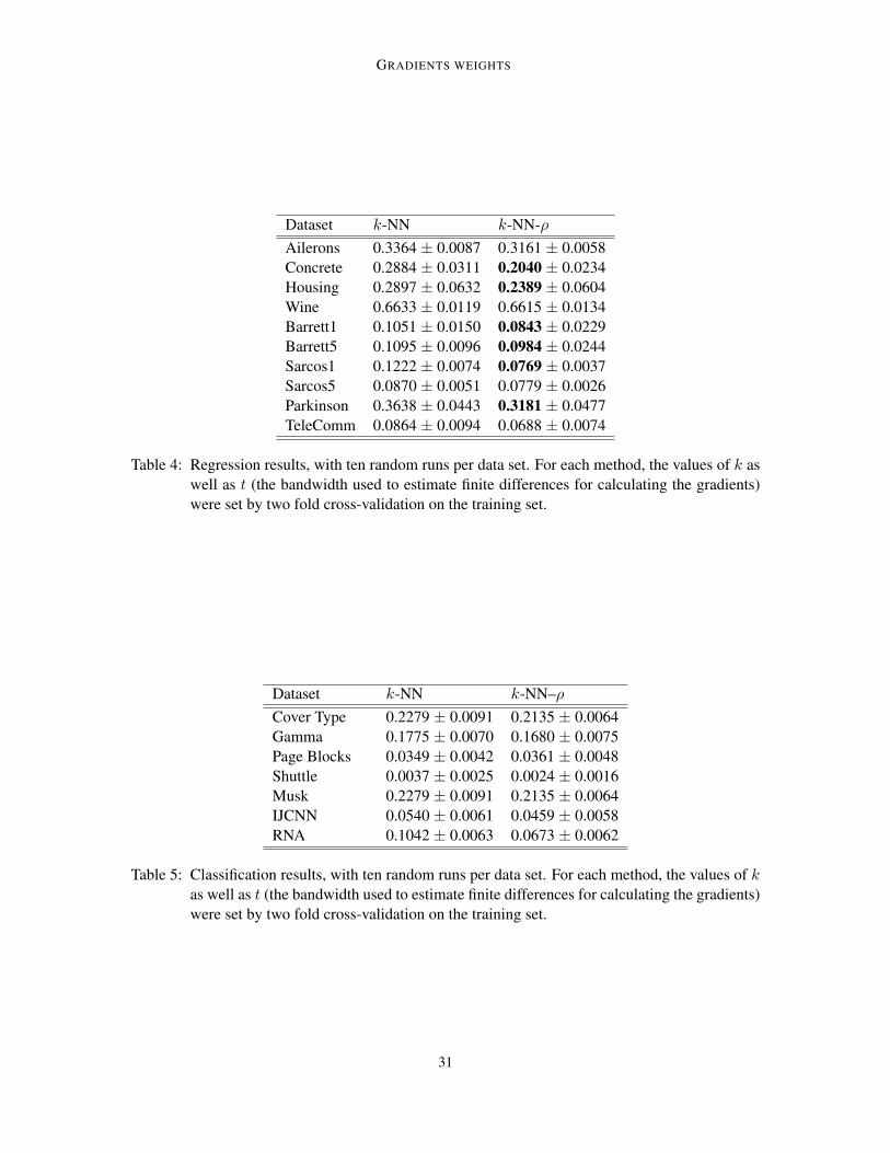
GRADIENTS WEIGHTS

Dataset k-NN k-NN-ρAilerons 0.3364 ± 0.0087 0.3161 ± 0.0058Concrete 0.2884 ± 0.0311 0.2040 ± 0.0234Housing 0.2897 ± 0.0632 0.2389 ± 0.0604Wine 0.6633 ± 0.0119 0.6615 ± 0.0134Barrett1 0.1051 ± 0.0150 0.0843 ± 0.0229Barrett5 0.1095 ± 0.0096 0.0984 ± 0.0244Sarcos1 0.1222 ± 0.0074 0.0769 ± 0.0037Sarcos5 0.0870 ± 0.0051 0.0779 ± 0.0026Parkinson 0.3638 ± 0.0443 0.3181 ± 0.0477TeleComm 0.0864 ± 0.0094 0.0688 ± 0.0074

Table 4: Regression results, with ten random runs per data set. For each method, the values of k aswell as t (the bandwidth used to estimate finite differences for calculating the gradients)were set by two fold cross-validation on the training set.

Dataset k-NN k-NN–ρCover Type 0.2279 ± 0.0091 0.2135 ± 0.0064Gamma 0.1775 ± 0.0070 0.1680 ± 0.0075Page Blocks 0.0349 ± 0.0042 0.0361 ± 0.0048Shuttle 0.0037 ± 0.0025 0.0024 ± 0.0016Musk 0.2279 ± 0.0091 0.2135 ± 0.0064IJCNN 0.0540 ± 0.0061 0.0459 ± 0.0058RNA 0.1042 ± 0.0063 0.0673 ± 0.0062

Table 5: Classification results, with ten random runs per data set. For each method, the values of kas well as t (the bandwidth used to estimate finite differences for calculating the gradients)were set by two fold cross-validation on the training set.

31


Barrett joint 1 Barrett joint 5 SARCOS joint 1 SARCOS joint 5 HousingKR error 0.50 ± 0.02 0.50 ± 0.03 0.16 ± 0.02 0.14 ± 0.02 0.37 ± 0.08KR-ρ error 0.38 ± 0.03 0.35 ± 0.02 0.14 ± 0.02 0.12 ± 0.01 0.25 ± 0.06KR-ρ2 error 0.30 ± 0.03 0.28 ± 0.03 0.11 ± 0.02 0.12 ± 0.01 0.21 ± 0.04KR-ρ3 error 0.18 ± 0.02 0.20 ± 0.01 0.18 ± 0.03 0.14 ± 0.02 0.25 ± 0.03KR-ρ4 error 0.17 ± 0.01 0.20 ± 0.01 0.37 ± 0.02 0.20 ± 0.01 0.39 ± 0.08KR time 0.39 ± 0.02 0.37 ± 0.01 0.28 ± 0.05 0.23 ± 0.03 0.10 ±0.01KR-ρ time 0.41 ± 0.03 0.38 ± 0.02 0.32 ± 0.05 0.23 ± 0.02 0.11 ±0.01

Concrete Strength Wine Quality Telecom Ailerons Parkinson’sKR error 0.42 ± 0.05 0.75 ± 0.03 0.30 ± 0.02 0.40 ± 0.02 0.38 ± 0.03KR-ρ error 0.37 ± 0.03 0.75 ± 0.02 0.23 ± 0.02 0.39 ± 0.02 0.34 ± 0.03KR-ρ2 error 0.31 ± 0.02 0.72 ± 0.02 0.37 ± 0.08 0.37 ± 0.02 0.34 ± 0.02KR-ρ3 error 0.28 ± 0.04 0.73 ± 0.03 0.57 ± 0.02 0.38 ± 0.02 0.31 ± 0.02KR-ρ4 error 0.37 ± 0.04 0.78 ± 0.02 0.54 ± 0.03 0.41 ± 0.01 0.30 ± 0.01KR time 0.14 ± 0.02 0.19 ± 0.02 0.15±0.01 0.20±0.01 0.30±0.03KR-ρ time 0.14 ± 0.01 0.19 ± 0.02 0.16±0.01 0.21±0.01 0.30±0.03

Barrett joint 1 Barrett joint 5 SARCOS joint 1 SARCOS joint 5 Housingk-NN error 0.41 ± 0.02 0.40 ± 0.02 0.08 ± 0.01 0.08 ± 0.01 0.28 ± 0.09k-NN-ρ error 0.29 ± 0.01 0.30 ± 0.02 0.07 ± 0.01 0.07 ± 0.01 0.22 ± 0.06k-NN-ρ2 error 0.21 ± 0.02 0.23 ± 0.01 0.06 ± 0.01 0.06 ± 0.01 0.18 ± 0.03k-NN-ρ3 error 0.11 ± 0.02 0.19 ± 0.01 0.08 ± 0.01 0.05 ± 0.01 0.23 ± 0.03k-NN-ρ4 error 0.15 ± 0.01 0.20 ± 0.01 0.37 ± 0.01 0.16 ± 0.01 0.31 ± 0.07k-NN time 0.21 ± 0.04 0.16 ± 0.03 0.13 ± 0.01 0.13 ± 0.01 0.08 ±0.01k-NN-ρ time 0.13 ± 0.04 0.16 ± 0.03 0.14 ± 0.01 0.13 ± 0.01 0.08 ±0.01

Concrete Strength Wine Quality Telecom Ailerons Parkinson’sk-NN error 0.40 ± 0.04 0.73 ± 0.04 0.13 ± 0.02 0.37 ± 0.01 0.22 ± 0.01k-NN-ρ error 0.38 ± 0.03 0.72 ± 0.03 0.17 ± 0.02 0.34 ± 0.01 0.20 ± 0.01k-NN-ρ2 error 0.31 ± 0.06 0.70 ± 0.01 0.34 ± 0.05 0.34 ± 0.01 0.20 ± 0.01k-NN-ρ3 error 0.26 ± 0.02 0.71 ± 0.01 0.55 ± 0.03 0.36 ± 0.01 0.22 ± 0.01k-NN-ρ4 error 0.38 ± 0.05 0.78 ± 0.01 0.52 ± 0.02 0.45 ± 0.01 0.25 ± 0.01k-NN time 0.10 ± 0.01 0.15 ± 0.01 0.16±0.02 0.12±0.01 0.14±0.01k-NN-ρ time 0.11 ± 0.01 0.15 ± 0.01 0.15±0.01 0.11±0.01 0.15±0.01

Table 6: Normalized mean square prediction errors and average prediction time per point (in mil-liseconds). The top five tables are for KR vs KR-ρ, KR-ρ2,KR-ρ3 and KR-ρ4, the bottomfive for k-NN vs k-NN-ρ, k-NN-ρ2, k-NN-ρ3 and k-NN-ρ4.

References

A. Beygelzimer, S. Kakade, and J. Langford. Cover trees for nearest neighbors. ICML, 2006.

Abdeslam Boularias, James Andrew Bagnell, and Anthony Stentz. Efficient Optimization for Au-tonomous Robotic Manipulation of Natural Objects. In Proceedings of the Twenty-Eighth AAAIConference on Artificial Intelligence, pages 2520–2526, 2014a.

32

GRADIENTS WEIGHTS

Abdeslam Boularias, James Andrew Bagnell, and Anthony Stentz. Robot Grasping DataSet. http://www.cs.rutgers.edu/˜ab1544/data/AAAI2014Data.tar.bz2.Carnegie Mellon University, Robotics Department, 2014b.

K. Clarkson. Nearest-neighbor searching and metric space dimensions. Nearest-Neighbor Methodsfor Learning and Vision: Theory and Practice, 2005.

Jason V. Davis, Brian Kulis, Prateek Jain, Suvrit Sra, and Inderjit S. Dhillon. Information-theoreticmetric learning. In ICML, pages 209–216, 2007.

L. Devroye, L. Gyorfi, and G. Lugosi. A Probabilistic Theory of Pattern Recognition. Springer,1996.

Rong-En Fan. LIBSVM Data: Classification, Regression, and Multi-label, 2012. URL http://www.csie.ntu.edu.tw/˜cjlin/libsvmtools/datasets/.

A. Frank and A. Asuncion. UCI machine learning repository. http://archive.ics.uci.edu/ml. University of California, Irvine, School of Information and Computer Sciences, 2012.

Haijie Gu and John Lafferty. Sequential nonparametric regression. arXiv preprint arXiv:1206.6408,2012.

L. Gyorfi, M. Kohler, A. Krzyzak, and H. Walk. A Distribution Free Theory of NonparametricRegression. Springer, New York, NY, 2002.

W. Hardle and T. Gasser. On robust kernel estimation of derivatives of regression functions. Scan-dinavian journal of statistics, pages 233–240, 1985.

Marc Hoffmann and Oleg Lepski. Random rates in anisotropic regression. Annals of statistics,pages 325–358, 2002.

Kenji Kira and Larry A. Rendell. A practical approach to feature selection. In Proceedings of theNinth International Workshop on Machine Learning, ML92, pages 249–256, 1992.

Igor Kononenko. Estimating attributes: Analysis and extensions of RELIEF. In Proc. EuropeanConf. on Machine Learning, pages 171–182, 1994.

S. Kpotufe. k-NN Regression Adapts to Local Intrinsic Dimension. NIPS, 2011.

S. Kpotufe and A. Boularias. Gradient weights help nonparametric regressors. NIPS, 2012.

J. Lafferty and L. Wasserman. Rodeo: Sparse nonparametric regression in high dimensions. Arxivpreprint math/0506342, 2005.

Duy Nguyen-Tuong and Jan Peters. Incremental online sparsification for model learning in real-timerobot control. Neurocomputing, 74(11):1859–1867, 2011.

Duy Nguyen-Tuong, Matthias W. Seeger, and Jan Peters. Model learning with local gaussian pro-cess regression. Advanced Robotics, 23(15):2015–2034, 2009.

M Nusbaum. Optimal filtration of a function of many variables in white gaussian noise. PROB.INFO. TRANSMISSION., 19(2):105–111, 1983.

33


Philippe Rigollet and Alexandre Tsybakov. Exponential screening and optimal rates of sparse esti-mation. The Annals of Statistics, 39(2):731–771, 2011.

Marko Robnik-Sikonja and Igor Kononenko. Theoretical and empirical analysis of relieff and rreli-eff. Machine learning, 53(1-2):23–69, 2003.

L. Rosasco, S. Villa, S. Mosci, M. Santoro, and A. Verri. Nonparametric sparsity and regularization.http://arxiv.org/abs/1208.2572, 2012.

Shai Shalev-shwartz, Yoram Singer, and Andrew Y. Ng. Online and batch learning of pseudo-metrics. In ICML, pages 743–750. ACM Press, 2004.

C. J. Stone. Optimal rates of convergence for non-parametric estimators. Ann. Statist., 8:1348–1360,1980.

C. J. Stone. Optimal global rates of convergence for non-parametric estimators. Ann. Statist., 10:1340–1353, 1982.

Yijun Sun. Iterative RELIEF for feature weighting: Algorithms, theories, and applications. IEEETrans. Pattern Analysis and Machine Intelligence, 29(6):1035–1051, 2007.

Luis Torgo. Regression datasets. http://www.liaad.up.pt/˜ltorgo. University of Porto,Department of Computer Science, 2012.

Shubhendu Trivedi, Jialei Wang, Samory Kpotufe, and Gregory Shakhnarovich. A consistent es-timator of the expected gradient outerproduct. In Proceedings of the Thirtieth Conference onUncertainty in Artificial Intelligence, pages 819–828, 2014.

V. Vapnik and A. Chervonenkis. On the uniform convergence of relative frequencies of events totheir expectation. Theory of probability and its applications, 16:264–280, 1971.

Kilian Q. Weinberger and Gerald Tesauro. Metric learning for kernel regression. Journal of MachineLearning Research - Proceedings Track, 2:612–619, 2007.

Dietrich Wettschereck, David W. Aha, and Takao Mohri. A review and empirical evaluation offeature weighting methods for a class of lazy learning algorithms. Artificial Intelligence Review,11:273–314, 1997.

Bo Xiao, Xiaokang Yang, Yi Xu, and Hongyuan Zha. Learning distance metric for regression bysemidefinite programming with application to human age estimation. In Proceedings of the 17thACM international conference on Multimedia, pages 451–460, 2009.

Yingbo Zhou, Utkarsh Porwal, Ce Zhang, Hung Q Ngo, Long Nguyen, Christopher Re, and VenuGovindaraju. Parallel feature selection inspired by group testing. In Z. Ghahramani, M. Welling,C. Cortes, N.D. Lawrence, and K.Q. Weinberger, editors, Advances in Neural Information Pro-cessing Systems 27, pages 3554–3562. Curran Associates, Inc., 2014.

34

Documents

Gradients Weights improve Regression and Classiﬁcationskk2175/Papers/jmlr2016.pdf · c 2016 Samory Kpotufe, Abdeslam Boularias, Thomas Schultz, and Kyoungok Kim. S. KPOTUFE, A