Embed Size (px)
Citation preview

Gradient-, Ensemble-, and Adjoint-FreeData-Driven Parameter Estimation
by
Ankit Goel
A dissertation submitted in partial fulfillmentof the requirements for the degree of
Doctor of Philosophy(Aerospace Engineering)
in The University of Michigan2019
Doctoral Committee:
Professor Dennis S. Bernstein, ChairProfessor Karthik DuraisamyAssistant Professor Alex GorodetskyProfessor Aaron Ridley

ACKNOWLEDGEMENTS
First and foremost, I would like to thank my advisor, Professor Dennis Bern-
stein for giving me the opportunity to work under his guidance during last several
years. This dissertation would not have been possible without his infallible support,
encouragement, and numerous memorable discussions. Also, I would like to thank
my committee members Professor Karthik Duraisamy, Professor Aaron Ridley, and
Professor Alex Gorodetsky for giving me challenging projects and providing helpful
comments and suggestions. I am extremely grateful for the opportunity to study at
the University of Michigan, and learn from some of the best professors.
I would like to also acknowledge all my friends and colleagues in Ann Arbor:
Sneha Sanjeevini, Ambarish Desai, Nitin Sharma, Pradyumna Srinivasan, Albert
Thomas, Sushant Choudhary, Pradeep Kumar, Ahmad Ansari, Ming-Jui (Ray) Yu,
Antai Xie, Khaled Aljanaideh, Yousaf Rahman, Frant Sobolic, Syed Aseem Ul Islam,
Adam Bruce, Angeline G. Burrell, Pedro Di Donato, Robert Zidek, Sweewarman
Balachandran, Gianluca Kapiris, Christian Spiess, who have made my time in the
graduate school very enjoyable.
Finally, I would like to thank my parents and my brother for their unconditional
love, support, and encouragement. I am very grateful for the family I have.
ii

TABLE OF CONTENTS
ACKNOWLEDGEMENTS . . . . . . . . . . . . . . . . . . . . . . . . . . ii
LIST OF FIGURES . . . . . . . . . . . . . . . . . . . . . . . . . . . . . . . vi
LIST OF TABLES . . . . . . . . . . . . . . . . . . . . . . . . . . . . . . . . x
ABSTRACT . . . . . . . . . . . . . . . . . . . . . . . . . . . . . . . . . . . xi
CHAPTER
1. Introduction . . . . . . . . . . . . . . . . . . . . . . . . . . . . . . 1
1.1 Motivation and Purpose . . . . . . . . . . . . . . . . . . . . . 11.2 Contributions . . . . . . . . . . . . . . . . . . . . . . . . . . . 91.3 Dissertation Outline . . . . . . . . . . . . . . . . . . . . . . . 101.4 Publications . . . . . . . . . . . . . . . . . . . . . . . . . . . 11
1.4.1 Journal Articles . . . . . . . . . . . . . . . . . . . . 121.4.2 Peer–reviewed Conference Papers . . . . . . . . . . 12
2. Gradient-, Ensemble-, and Adjoint-Free Data-Driven Param-eter Estimation . . . . . . . . . . . . . . . . . . . . . . . . . . . . . 14
2.1 Introduction . . . . . . . . . . . . . . . . . . . . . . . . . . . 142.2 Parameter-Estimation Problem . . . . . . . . . . . . . . . . . 172.3 Retrospective Cost Parameter Estimation . . . . . . . . . . . 20
2.3.1 Parameter Estimator . . . . . . . . . . . . . . . . . 202.3.2 Retrospective Cost Optimization . . . . . . . . . . . 22
2.4 Analysis of RCPE . . . . . . . . . . . . . . . . . . . . . . . . 242.4.1 The filter Gf . . . . . . . . . . . . . . . . . . . . . . 24
2.5 Examples with lµ = ly = 1 . . . . . . . . . . . . . . . . . . . . 272.6 Example with lµ = ly = 2 . . . . . . . . . . . . . . . . . . . . 332.7 Examples with lµ = 2 and ly = 1 . . . . . . . . . . . . . . . . 362.8 Examples with lµ = 3 and ly = 1 . . . . . . . . . . . . . . . . 412.9 Parameter Estimation in the Generalized Burgers Equation . 52
iii

2.10 Thermal Conductivity Estimation using Density Measurements 552.11 Conclusions . . . . . . . . . . . . . . . . . . . . . . . . . . . . 59
3. Estimation of the Eddy Diffusion Coefficient Using Total Elec-tron Content Data . . . . . . . . . . . . . . . . . . . . . . . . . . . 60
3.1 Introduction . . . . . . . . . . . . . . . . . . . . . . . . . . . 603.2 Global Ionosphere-Thermosphere Model . . . . . . . . . . . . 623.3 Retrospective Cost Parameter Estimation . . . . . . . . . . . 63
3.3.1 Retrospective Cost Optimization . . . . . . . . . . . 653.4 Biquadratic Retrospective Cost Optimization . . . . . . . . . 66
3.4.1 Retrospective cost as a quadratic function of θ . . . 673.4.2 Retrospective cost as a quadratic function of N . . 673.4.3 Alternating Convex Search algorithm . . . . . . . . 70
3.5 Illustrative example . . . . . . . . . . . . . . . . . . . . . . . 713.6 Estimation of EDC using TEC GITM . . . . . . . . . . . . . 753.7 Conclusions . . . . . . . . . . . . . . . . . . . . . . . . . . . . 78
4. Recursive Least Squares with Information-Driven DirectionalForgetting . . . . . . . . . . . . . . . . . . . . . . . . . . . . . . . . 79
4.1 Recursive Least Squares . . . . . . . . . . . . . . . . . . . . . 824.2 Persistent Excitation and Forgetting . . . . . . . . . . . . . . 884.3 Persistent Excitation and the Condition Number . . . . . . . 964.4 Lyapunov Analysis of the Parameter Error . . . . . . . . . . 1004.5 Lack of Persistent Excitation . . . . . . . . . . . . . . . . . . 1084.6 Information Subspace . . . . . . . . . . . . . . . . . . . . . . 1144.7 Information-Driven Forgetting . . . . . . . . . . . . . . . . . 1174.8 Conclusions . . . . . . . . . . . . . . . . . . . . . . . . . . . . 124
5. Adaptive Squaring-Based Control Allocation for Wide Systems125
5.1 Introduction . . . . . . . . . . . . . . . . . . . . . . . . . . . 1255.2 Control allocation problem . . . . . . . . . . . . . . . . . . . 1275.3 RCAC algorithm . . . . . . . . . . . . . . . . . . . . . . . . . 128
5.3.1 Retrospective Performance Variable . . . . . . . . . 1295.3.2 Retrospective Cost Function . . . . . . . . . . . . . 1305.3.3 The Target Model Gf . . . . . . . . . . . . . . . . . 131
5.4 Illustrative Examples . . . . . . . . . . . . . . . . . . . . . . 1335.4.1 Colocated actuators . . . . . . . . . . . . . . . . . . 1345.4.2 Independent actuators . . . . . . . . . . . . . . . . 1355.4.3 Uncontrollable channels . . . . . . . . . . . . . . . . 137
5.5 Conclusions . . . . . . . . . . . . . . . . . . . . . . . . . . . . 138
iv

6. Output-Constrained Adaptive Control for Unstart Preven-tion in a 2D Scramjet Combustor . . . . . . . . . . . . . . . . . 140
6.1 Introduction . . . . . . . . . . . . . . . . . . . . . . . . . . . 1406.2 Scramjet Model . . . . . . . . . . . . . . . . . . . . . . . . . 1426.3 Unstart and Unstart detection . . . . . . . . . . . . . . . . . 1446.4 Adaptive Setpoint Command Following . . . . . . . . . . . . 1466.5 Adaptive Command Following with Conflicting Commands . 1476.6 Adaptive Command Following with Auxiliary Output Con-
straints . . . . . . . . . . . . . . . . . . . . . . . . . . . . . . 1546.7 Conclusions . . . . . . . . . . . . . . . . . . . . . . . . . . . . 159
7. Conclusions and Future Work . . . . . . . . . . . . . . . . . . . 161
BIBLIOGRAPHY . . . . . . . . . . . . . . . . . . . . . . . . . . . . . . . . 165
v

LIST OF FIGURES
Figure
1.1 Mass-spring system with unknown spring stiffness . . . . . . . . . . 2
2.1 Retrospective cost parameter estimation. . . . . . . . . . . . . . . 20
2.2 The set SOp for lµ = 2. . . . . . . . . . . . . . . . . . . . . . . . . . 22
2.3 Estimation of unknown parameters in an affinely parameterized linearsystem. . . . . . . . . . . . . . . . . . . . . . . . . . . . . . . . . . 28
2.4 Effect of the choice of input and filter coefficient. . . . . . . . . . . . 29
2.5 Effect of initial conditions on convergence. . . . . . . . . . . . . . . 30
2.6 Estimation of unknown parameters in a nonaffinely parameterizedlinear system. . . . . . . . . . . . . . . . . . . . . . . . . . . . . . . 31
2.7 UKF-based parameter estimation. . . . . . . . . . . . . . . . . . . 32
2.8 Effect of noise on the estimation accuracy of (a) RCPE and (b) UKF. 33
2.9 Estimation of unknown parameters in a nonaffinely parameterizedlinear system. . . . . . . . . . . . . . . . . . . . . . . . . . . . . . . 34
2.10 Estimation of unknown parameters in a nonaffinely parameterizedlinear system using sparse integrator. . . . . . . . . . . . . . . . . . 35
2.11 Estimation of unknown parameters in an affinely parameterized linearsystem. . . . . . . . . . . . . . . . . . . . . . . . . . . . . . . . . . 37
2.12 Parameter pre-estimate ν(k) for various choices of Gf . . . . . . . . . 38
vi
2.13 Estimation of unknown parameters in a nonaffinely parameterizedlinear system. . . . . . . . . . . . . . . . . . . . . . . . . . . . . . . 40
2.14 Parameter pre-estimate ν(k) for various choices of Gf . . . . . . . . 41
2.15 Estimation of unknown parameters in an affinely parameterized linearsystem. . . . . . . . . . . . . . . . . . . . . . . . . . . . . . . . . . 42
2.16 Parameter pre-estimate ν(k) for various choices of Gf and Op . . . . 44
2.17 Parameter pre-estimate ν(k) for various choices of Gf and Op. . . . 46
2.18 Estimation of unknown parameters in a nonaffinely parameterizedlinear system. . . . . . . . . . . . . . . . . . . . . . . . . . . . . . . 48
2.19 Output error for all six permutations. . . . . . . . . . . . . . . . . . 49
2.20 Parameter pre-estimate ν(k) for various choices of Gf and Op. . . . 51
2.21 Simulation of the generalized Burgers equation with the discretization(2.57). . . . . . . . . . . . . . . . . . . . . . . . . . . . . . . . . . . 54
2.22 Estimation of unknown parameters in the generalized Burgers equa-tion. . . . . . . . . . . . . . . . . . . . . . . . . . . . . . . . . . . . 55
2.23 Estimation of thermal conductivity coefficients. . . . . . . . . . . . 57
2.24 Effect of the initial parameter guess on the estimates of thermal con-ductivity coefficients. . . . . . . . . . . . . . . . . . . . . . . . . . 58
3.1 RCPE estimate of the unknown parameter µ in the linear system(3.37), (3.38) with the nonlinear parameter dependence (3.39)-(3.41). 73
3.2 Effect of the ACS filter initialization N0 and the weight Rθ on theperformance of RCPE. . . . . . . . . . . . . . . . . . . . . . . . . . 74
3.3 RCPE estimate of the unknown EDC in GITM. . . . . . . . . . . . 76
3.4 Measured and computed TEC at the fictitious ground station locatedat 1 deg North, 45 deg East. . . . . . . . . . . . . . . . . . . . . . 77
4.1 Example 4.2. Persistent excitation and bounds on P−1k . . . . . . . 94
4.2 Example 4.3. Lack of persistent excitation and bounds on P−1k . . . 95
vii

4.3 Example 4.4. Using the condition number of Pk to evaluate persis-tency. . . . . . . . . . . . . . . . . . . . . . . . . . . . . . . . . . . 99
4.4 Example 4.5. Effect of λ on the rate of convergence of θk. . . . . . 107
4.5 Example 4.7. Subspace constrained regressor. . . . . . . . . . . . . 110
4.6 Example 4.7. Subspace constrained regressor. . . . . . . . . . . . . 111
4.7 Example 4.8. Effect of lack of persistent excitation on θk. . . . . . 113
4.8 Illustrative example of the information subspace. . . . . . . . . . . . 115
4.10 Example 4.10. Information-driven forgetting for a regressor lackingpersistent excitation. . . . . . . . . . . . . . . . . . . . . . . . . . . 121
4.11 Example 4.11. Effect of Information-driven forgetting on θk. . . . . 122
4.9 Example 4.9. Relation between Pk and the information content ψk. 123
5.1 Block diagram representation of the adaptive control allocation prob-lem with the adaptive controller Gc and plant G. . . . . . . . . . . 128
5.2 Example 5.4.1. Control allocation for setpoint command following. 135
5.3 Example 5.4.2. Control allocation for setpoint command following. 136
5.4 Example 5.4.3. Control allocation for setpoint command following. 138
6.1 Geometry of the Hyshot-II scramjet engine. . . . . . . . . . . . . . . 143
6.2 Critical thrust y0 and the pressure metric pm in the normal operatingand unstarting scramjet. . . . . . . . . . . . . . . . . . . . . . . . . 146
6.3 Scramjet command-following control system architecture . . . . . . 147
6.4 Closed-loop response of the spring-mass-damper system with conflict-ing commands. . . . . . . . . . . . . . . . . . . . . . . . . . . . . . 150
6.5 Asymptotic output of the spring-mass-damper system with conflict-ing commands for various filter and performance weight choices. . . 151
6.6 Closed-loop response of the scramjet to conflicting commands. . . . 152
viii

6.7 Closed-loop response of the scramjet to conflicting commands forvarious filter choices. . . . . . . . . . . . . . . . . . . . . . . . . . . 153
6.8 Closed-loop response of the system (6.19), (6.20) with auxiliary out-put constraints. . . . . . . . . . . . . . . . . . . . . . . . . . . . . . 157
6.9 Closed-loop response of the scramjet with the auxiliary output con-straint. . . . . . . . . . . . . . . . . . . . . . . . . . . . . . . . . . 159
ix

LIST OF TABLES
Table
2.1 Summary of the numerical examples. . . . . . . . . . . . . . . . . . 17
2.2 Filter coefficients for Example 2.4. . . . . . . . . . . . . . . . . . . 38
2.3 Filter coefficients and Op for Example 2.6. . . . . . . . . . . . . . . 43
2.4 Filter coefficient sign for Example 2.6. . . . . . . . . . . . . . . . . 45
2.5 Filter coefficients and Op for Example 2.7. . . . . . . . . . . . . . . 50
4.1 Summary of definitions, results, and examples in this chapter. . . . 81
4.2 Various expressions for RLS variables. . . . . . . . . . . . . . . . . . 88
4.3 Behavior of Pk under persistent and not persistent excitation. . . . . 96
4.4 Asymptotic behavior of RLS in Example 4.6. In the case of persistentexcitation with λ < 1, the convergence of θk is geometric. . . . . . . 109
6.1 Summary of parameters used in the heat-release model (6.3), (6.4). 144
x

ABSTRACT
In many applications, models of physical systems have known structure but un-
known parameters. By viewing the unknown parameters as constant states, nonlinear
estimation methods such as the extended Kalman filter, unscented Kalman filter, and
ensemble Kalman filter can be used to estimate the states of the augmented system,
thereby providing estimates of the parameters along with the dynamic states. These
methods tend to be computationally expensive due to the need for Jacobians, ensem-
bles, or adjoints, especially when the models are high-dimensional.
This dissertation presents retrospective cost parameter estimation (RCPE), which
does not require gradients, ensembles, or adjoints. Rather, RCPE estimates unknown
parameters from a single trajectory, and requires updating an adaptive integrator gain
for each unknown parameter. RCPE is applicable to parameter estimation in linear
and nonlinear models, where the parameterization may be either affine or nonaffine.
The main contribution of this work is to show that the parameter estimates may
be permuted in an arbitrary way, and thus a permutation is needed to correctly as-
sociate each parameter estimate with the corresponding unknown parameter. RCPE
is illustrated through several numerical examples including the Burgers equation and
the Global Ionosphere Thermosphere Model (GITM), where the goal is to estimate
representational parameters such as eddy diffusion coefficient and thermal conduc-
tivity coefficients using measurements of atmospheric variables such as total electron
content, density, temperatures etc.
The next part of the dissertation focuses on forgetting in the context of recursive
least squares (RLS) algorithm. It is a well-known fact that classical RLS with for-
xi

getting diverges in the cases where the excitation is not persistent. In this work, an
information-driven directional forgetting technique is proposed, which constrains the
forgetting to directions in which new information is available, thereby allowing RLS
to operate without divergence during periods of loss of persistency.
In the last part of this dissertation, retrospective cost adaptive control (RCAC)
is extended to the problem of control allocation in overactuated systems. In partic-
ular, it is shown that the applied control input lies in the range of the target model
used in RCAC, thereby providing a simple technique to constrain the control input
to a desired subspace. Finally, RCAC is extended to asymptotically enforce output
constraint by formulating the problem as a problem of following conflicting com-
mands, and is used to prevent a scramjet combustor from unstarting using pressure
measurements.
xii

CHAPTER 1
Introduction
1.1 Motivation and Purpose
In many applications of science and engineering, models of physical systems have
known structure but unknown parameters. In such models, often called gray-box
models, the structure of the function describing the evolution of the state of the system
is known, but the values of the parameters in the function may be unknown. These
parameters might be embedded in the model in such a way that direct calculation is
not possible due to lack of measurements. Such parameters are called inaccessible,
which means that they relate unmeasured signals, and thus cannot be determined by
regression. Furthermore, these parameters might represent the cumulative effect of a
complex phenomena, and thus might not have a true measurable value.
To illustrate this problem, consider the problem of estimating the spring stiffness
k2 in the mass-spring system shown in Figure 1.1. The system is modeled by
m1q1 + (k1 + k2)q1 − k2q2 = 0, (1.1)
m2q2 − k2q1 + k2q2 = F, (1.2)
where q1 is the position of the mass m1, q2 is the position of the mass m2, and k1, k2
are the stiffness of the first and second spring, and F is the force applied to m2. Note
1
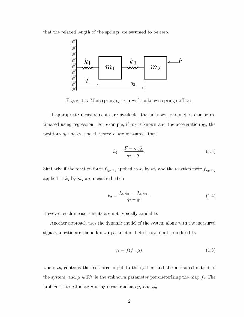
that the relaxed length of the springs are assumed to be zero.
m1 m2k1 k2
q1 q2
F
Figure 1.1: Mass-spring system with unknown spring stiffness
If appropriate measurements are available, the unknown parameters can be es-
timated using regression. For example, if m2 is known and the acceleration q2, the
positions q1 and q2, and the force F are measured, then
k2 =F −m2q2q2 − q1
. (1.3)
Similarly, if the reaction force fk2/m1 applied to k2 by m1 and the reaction force fk2/m2
applied to k2 by m2 are measured, then
k2 =fk2/m1 − fk2/m2
q2 − q1. (1.4)
However, such measurements are not typically available.
Another approach uses the dynamic model of the system along with the measured
signals to estimate the unknown parameter. Let the system be modeled by
yk = f(φk, µ), (1.5)
where φk contains the measured input to the system and the measured output of
the system, and µ ∈ Rlµ is the unknown parameter parameterizing the map f . The
problem is to estimate µ using measurements yk and φk.
2

The most common approach is to use least-squares formulation to estimate the
unknown parameter. In this case, the estimate µk of the unknown parameter µ at
step k is given by the minimizer of
J(µ)4=
k∑i=0
(yi − yi)T(yi − yi), (1.6)
where yi is the computed output of the estimation model given by
yi = f(φi, µ). (1.7)
for all i ∈ {0, 1, · · · , k}.
If the model (1.5) is linearly parameterized by µ, that is, the output yk can be
written as yk = φkµ, then the minimizer of (1.6) has a closed-form solution [1]. In
the case where f is nonlinearly parameterized by µ, using analytical expression of
f , [2] uses Taylor series expansion to iteratively minimize J(µ), [3] uses gradient-
descent method to minimize J(µ), while [4] optimally interpolates the solution given
by the Taylor series expansion and the gradient-descent method. The severity of
nonlinearity in function f and the order of the system (1.5) render minimization of
J(µ) using anylytical methods difficult. In addition, these methods are plagued by
slow convergence or divergence of the estimates. Note that these methods require an
analytical expression of f to compute the gradients. Furthermore, the computational
cost increases with k.
In the case where analytical expression of f is not available, the gradient of the
cost function (1.6) can be computed by finite differences. Note that this method uses
f as a black-box model. However, this method becomes computationally expensive
as the size of the vector µ and the number of samples k increase. Alternatively, the
gradient of the cost function (1.6) can be computed by variational methods [5–7],
which require an adjoint formulation of the dynamics. Adjoint based methods tend
3

to be computationally expensive due to the need for multiple iterations of the forward
model and backward adjoint. To use the adjoint method to compute the gradient,
note that
dJ
dµ=
k∑i=0
∂J
∂yi
∂yi∂µ
(1.8)
For i ∈ {0, 1, · · · , k}, define gi(yi, µ)4= yi − f(φi, µ). Note that gi(yi, µ) = 0. Thus,
∂gi∂yi
∂yi∂µ
+∂gi∂µ
= 0. (1.9)
It follows from (1.8) and (1.9) that
dJ
dµ=
k∑i=0
λTi∂gi∂µ
. (1.10)
where λi is obtained by solving
∂gi∂yi
T
λi = − ∂J∂yi
T
. (1.11)
Note that (1.11) is called the adjoint equation. Various formulations based on adjoint
method to estimate unknown parameter in a dynamical system modeled using state-
space representation are discussed in [8–12].
As a special case of this problem, a linear system may have uncertain entries
in its state space representation. For this problem, a two-step procedure is used in
[13], where a black-box model is first constructed based on the input-output data,
and a similarity transformation is used to recover the unknown parameters. In [14],
a sequential convex relaxation method is used to estimate unknown entries in the
matrices of a state space realization.
The measurements of uk and yk may be corrupted by noise. In presence of noise,
4

the unknown parameter µ is treated as a random variable in a probabilistic frame-
work. Consequently, the statistical characteristics of µk depend on the the statistical
characteristics of the noise. In such cases, the parameter estimation problem has a
Bayesian interpretation. Using Bayes’ rule, the conditional probability distribution
of the unknown parameter given the measurements is formulated and maximized in
order to obtain the parameter estimate µk [5, 15–17]. In [18], parameters in the spe-
cial case of a linear system are estimated using expectation maximization algorithm
under the assumption of Gaussian noise.
State estimation techniques provide another framework for estimating the un-
known parameters. In this framework, (1.5) is written in the state-space form as
xk+1 = f(xk, uk, µ), (1.12)
yk = g(xk, uk, µ), (1.13)
where xk ∈ Rlx is the state of the system at step k, uk ∈ Rlu is the input to the
system, yk ∈ Rly is the measured output of the system, and µ ∈ Rlµ is the unknown
parameter parameterizing the dynamics map f and g. Usually, the state xk of the
system (1.12) is not available to estimate µ. By viewing the unknown parameters as
constant states, and augmenting the original states with the constant states, state
estimation techniques can be used to estimate the states of the augmented system,
thereby providing estimates of the parameters along with the dynamic states [19].
However, the parameter states multiply the dynamic states, thus the resulting esti-
mation dynamics are nonlinear irrespective of whether the “original” dynamics (1.12),
(1.13) are linear or nonlinear. Consequently, nonlinear state estimation techniques
such as the extended Kalman filter (EKF), unscented Kalman filter (UKF), and en-
semble Kalman filter (EnKF) can be applied to these problems [19–25]. For example,
to estimate k2 in (1.1), (1.2) using Kalman filter based estimation techniques, the
5
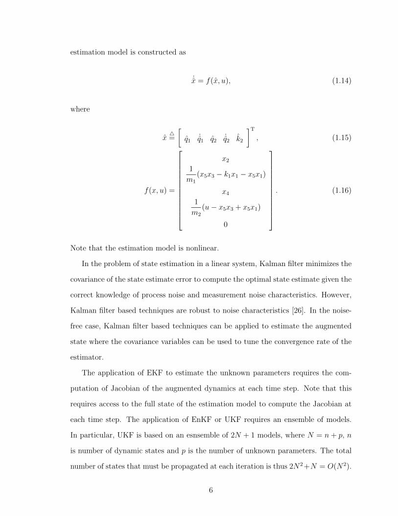
estimation model is constructed as
˙x = f(x, u), (1.14)
where
x4=
[q1 ˙q1 q2 ˙q2 k2
]T, (1.15)
f(x, u) =
x21
m1
(x5x3 − k1x1 − x5x1)
x41
m2
(u− x5x3 + x5x1)
0
. (1.16)
Note that the estimation model is nonlinear.
In the problem of state estimation in a linear system, Kalman filter minimizes the
covariance of the state estimate error to compute the optimal state estimate given the
correct knowledge of process noise and measurement noise characteristics. However,
Kalman filter based techniques are robust to noise characteristics [26]. In the noise-
free case, Kalman filter based techniques can be applied to estimate the augmented
state where the covariance variables can be used to tune the convergence rate of the
estimator.
The application of EKF to estimate the unknown parameters requires the com-
putation of Jacobian of the augmented dynamics at each time step. Note that this
requires access to the full state of the estimation model to compute the Jacobian at
each time step. The application of EnKF or UKF requires an ensemble of models.
In particular, UKF is based on an esnsemble of 2N + 1 models, where N = n+ p, n
is number of dynamic states and p is the number of unknown parameters. The total
number of states that must be propagated at each iteration is thus 2N2+N = O(N2).
6

Consequently, for a system with n dynamic states and p unknown parameters, it fol-
lows that N = n + p, and thus the total number of states that must be propagated
at each iteration is (2N + 1)N = [2(n+ p) + 1](n+ p). Note that UKF also requires
access to the full state of the estimation model to construct the ensemble.
The purpose of this dissertation is to present a gradient free, ensemble free, and ad-
joint free data driven parameter estimation technique. In particular, this dissertation
presents retrospective cost parameter estimation (RCPE) algorithm for estimating
multiple unknown parameters in linear and nonlinear systems with affine or nonaffine
parameterizations.
Like UKF but unlike EKF, RCPE does not require a Jacobian of the dynamics
in order to update the parameter estimates. However, unlike UKF, RCPE does not
require an ensemble of models. In contrast to UKF, RCPE requires the propagation
of only a single copy of the “original” system dynamics, so that the number of states
that must be propagated at each iteration is simply n. In addition, unlike EKF and
UKF, RCPE does not require access to the states of the estimation model. For
both UKF and RCPE, this model need only be given as an executable simulation;
explicit knowledge of the equations and source code underlying the simulation is not
required. Finally, unlike variational methods, RCPE does not require an adjoint
model. However, the price paid for not requiring an explicit model or an ensemble
of models is the need within RCPE to select a permutation matrix that correctly
associates each parameter estimate with the corresponding unknown parameter.
7

The retrospective cost parameter estimation algorithm is a variation of retrospec-
tive cost model refinement (RCMR) developed in [27–29] and is based on retrospective
cost adaptive control (RCAC) [30]. RCMR was developed to estimate unknown pa-
rameters in an affinely parameterized dynamical system. To estimate µ using RCMR,
(1.12) is written as
xk+1 = f(xk, uk) +
lµ∑i=1
vi,k, (1.17)
vi,k = µiwi,k, (1.18)
wi,k = hi(xk, uk). (1.19)
Note that µi appears as a static feedback in the dynamics given by (1.17). RCMR
minimizes a retrospective cost function based on the measurements of vi,k and wi,k
whose minimizer provides the parameter estimate µk. Although RCMR does not use
hi(xk, uk) to compute the estimate µk, RCMR does require that the function hi(xk, uk)
be available to compute wi,k. These requirements prohibits RCMR to be applicable
to problems where the dynamics (1.12) is nonlinearly parameterized or the dynamics
(1.12) are so complicated that construction of the functions hi(xk, uk) is cumbersome.
On the other hand, RCPE is applicable to parameter estimation in linear and
nonlinear models, where the parameterization may be either affine or nonaffine. In
order to update the parameter estimate, RCPE uses an error signal given by the
difference between the output of the system and the output of the estimation model.
The parameter update is obtained by minimizing a retrospective cost function whose
minimizer provides an update of the gains of an integrator. The output of the adaptive
integrator consists of the parameter pre-estimates, whose absolute values are the
parameter estimates. However, the parameter estimates may be permuted in an
unknown way, and thus a permutation is needed to correctly associate each parameter
estimate with the corresponding unknown parameter.
8

1.2 Contributions
The major contributions of the dissertation are listed below.
1. Development of RCPE, which is a gradient-, ensemble-, and adjoint-free data
driven parameter estimation algorithm applicable to affinely or nonaffinely pa-
rameterized systems.
2. Analysis of the retrospective cost in RCPE to show that the parameter estimate
is constrained to the subspace defined by the filter coefficients used to define
the retrospective cost.
3. Systematic demonstration of RCPE on low-order systems and high-dimensional
systems such as the Burgers equation and the global ionosphere thermosphere
model to show the effect of the ordering of the filter coefficients and the necessity
of the permutation matrix.
4. Formulation of the biquadratic retrospective cost to simultaneously optimize
the adaptive integrator gains and the filter coefficients in RCPE.
5. Analysis of asymptotic convergence of recursive least squares algorithm using
discrete-time Lyapunov theory and asymptotic bounds on RLS variables under
persistent excitation.
6. Development of the information-driven directional forgetting scheme in recur-
sive least squares algorithm to constrain forgetting to the information subspace
in the case of lack of persistent excitation.
7. Extension of RCAC to constrain the input to a desired input subspace and
application to the problem of control allocation in wide systems.
8. Extension of RCAC to enforce output constrains asymptotically and application
to a 2D scramjet combustor to prevent unstart.
9

1.3 Dissertation Outline
This disseration is organized as follows.
Chapter 2 Summary
Chapter 2 presents the parameter estimation problem in dynamical systems. First,
The parameter estimator, consisting of an adaptive integrator, permutation, and a
nonlinear transformation to the first orthant is presented. Then, the retrospective cost
parameter estimation (RCPE) algorithm is presented. Next, it is shown in Theorem
2.1 that the parameter estimates produced by RCPE are constrained to lie in a
subspace defined by the filter coefficients that define the retrospective cost. Then,
the need of permutation is shown through several numerical examples. Finally, RCPE
is applied to high-dimensional nonlinear systems.
Chapter 3 Summary
Chapter 3 extends RCPE by simultaneously optimizing the the filter coefficients
that define the retrospective cost. It is shown that that the optimization problem is
biquadratic but nonconvex. An alternating convex search is used to converge to a local
minimizer. The extended algorithm is demonstrated on a low-dimensional system,
and finally, it is used to estimate eddy diffusion coefficient (EDC) in global ionosphere-
thermosphere model (GITM) by using measurements of total electron content (TEC).
Chapter 4 Summary
Chapter 4 presents a novel directional forgetting algorithm to prevent estimator
divergence under lack of persistency in the context of recursive least squares. Various
results on the effect of forgetting with and without the persistence of excitation are
10

presented, and it is shown that some singular values of the covariance matrix diverge
in the case where excitation is not persistent. Finally, a matrix forgetting scheme is
proposed which constrains forgetting to the directions receiving new information.
Chapter 5 Summary
Chapter 5 presents the control allocation problem. In the context of the retro-
spective cost adaptive control (RCAC), it is shown that the the control input lies in
the range of the target model. An extension of Theorem 2.1 that includes control
penalty in the retrospective cost is presented. Finally, numerical examples demon-
strate control allocation in wide plant using RCAC.
Chapter 6 Summary
Chapter 6 extends RCAC to enforce auxiliary output constraints. First, it is shown
that in the case of conflicting commands, RCAC trades off output error based on the
choice of the target model. Next, the problem of output constraints is formulated as
a command-following problem with conflicting commands. Although the constraint
is violated, it is shown that the asymptotic magnitude of the constraint violation
error can be arbitrarily reduced by tuning the target model in RCAC. Finally, the
extended RCAC algorithm is used to prevent unstart in a two-dimensional scramjet
combustor model.
Finally, the thesis is concluded in Chapter 7.
1.4 Publications
The following is the list of publications relevant to the research presented in this
dissertation.
11

1.4.1 Journal Articles
• A. Goel, and D. S. Bernstein, “Gradient-, Ensemble-, and Adjoint-Free Data-
Driven Parameter Estimation”, Accepted for publication in AIAA Journal of
Guidance, Control, and Dynamics.
• A. Goel, and D. S. Bernstein, ” Recursive Least Squares with Directional For-
getting”, submitted to IEEE Control System Magazine.
• A. Goel, K. Duraisamy, and D. S. Bernstein, ”Retrospective Cost Adaptive
Control of Unstart in a Model Scramjet Combustor”, AIAA Journal, vol. 56,
no. 3, pp. 1085–1096, 2018.
• A. G. Burrell, A. Goel, A. J. Ridley, and D. S. Bernstein, “Correction of the
Photoelectron Heating Efficiency Within the Global Ionosphere-Thermosphere
Model Using Retrospective Cost Model Refinement”, Journal of Atmospheric
Solar-Terrestrial Physics, Vol. 124, pp. 30–38, 2015.
1.4.2 Peer–reviewed Conference Papers
• A. Goel and D. S. Bernstein, “Data-Driven Parameter Estimation for Mod-
els with Nonlinear Parameter Dependence,” in Proceedings of Conference on
Decision and Control, pp. 1470–1475, Miami, FL, Dec 2018.
• A. Goel , K. Duraisamy, and D. S. Bernstein, ”Output-Constrained Adaptive
Control for Unstart Prevention in a 2D Scramjet Combustor ,” AIAA Scitech
2019 Forum , San Diego, CA, Jan 2019.
• A. Goel, A. Ansari and D. S. Bernstein, “Adaptive Squaring-Based Control
Allocation for Wide Systems with Application to Lateral Flight Control,” in
Proceedings of Conference on Decision and Control, pp. 5140–5145, Miami,
FL, Dec 2018.
12
• A. Goel and D. S. Bernstein, “A Targeted Forgetting Factor for Recursive Least
Squares,” in Proceedings of Conference on Decision and Control, pp. 3899–
3903, Miami, FL, Dec 2018.
• A. Goel and D. S. Bernstein, “Parameter Estimation for Nonlinearly Parame-
terized Gray-Box Models,” in Proceedings of American Control Conference, pp.
5280–5285, Milwaukee, WI, June 2018.
• A. Goel, A. Ridley, and D. S. Bernstein, “Estimation of the Eddy Diffusion
Coefficient Using Total Electron Content Data,” in Proceedings of American
Control Conference, pp. 3298–3303, Milwaukee, WI, June 2018.
• A. Goel, K. Duraisamy and D. S. Bernstein, “Parameter estimation in the
Burgers equation using retrospective-cost model refinement,“ in Proceedings of
American Control Conference, pp. 6983–6988, Boston, MA, July 2016.
13
CHAPTER 2
Gradient-, Ensemble-, and Adjoint-Free
Data-Driven Parameter Estimation
2.1 Introduction
In many applications, models of physical systems have known structure but un-
known parameters. By viewing the unknown parameters as constant states, nonlin-
ear estimation methods can be used to estimate the states of the augmented system,
thereby providing estimates of the parameters along with the dynamic states [19].
The extended Kalman filter (EKF), unscented Kalman filter (UKF), and ensemble
Kalman filter (EnKF) can be applied to these problems [19–25]. An alternative ap-
proach to parameter estimation is variational methods [6, 7, 31], which require an
adjoint formulation of the dynamics, These methods tend to be computationally ex-
pensive due to the need for multiple iterations of the forward model and backward
adjoint.
As a special case of this problem, a linear system may have uncertain entries in its
state space representation. Since the parameter states multiply the dynamic states,
the resulting estimation dynamics are nonlinear despite the fact that the “original”
dynamics are linear. For this problem, a two-step procedure is used in [13], where a
black-box model is first constructed based on the input-output data, and a similarity
14

transformation is used to recover the unknown parameters. In [14], a sequential
convex relaxation method is used to estimate unknown entries in the matrices of a
state space realization.
The present chapter focuses on retrospective cost parameter estimation (RCPE),
which is a variation of retrospective cost model refinement (RCMR) developed in
[27–29] and is based on retrospective cost adaptive control [30]. RCPE is applicable
to parameter estimation in linear and nonlinear models, where the parameterization
may be either affine or nonaffine. In order to update the parameter estimate, RCPE
uses an error signal given by the difference between the output of the physical sys-
tem and the output of the estimation model. The parameter update is obtained by
minimizing a retrospective cost function whose minimizer provides an update of the
gains of an integrator. The output of the adaptive integrator consists of the pa-
rameter pre-estimates, whose absolute values are the parameter estimates. However,
the parameter estimates may be permuted in an unknown way, and thus a permuta-
tion is needed to correctly associate each parameter estimate with the corresponding
unknown parameter.
Like UKF but unlike EKF, RCPE does not require a Jacobian of the dynamics
in order to update the parameter estimates. However, unlike UKF, RCPE does not
require an ensemble of models. In particular, for parameter estimation, the unscented
Kalman filter (UKF) is based on an ensemble of 2N + 1 models, where N = n+ p, n
is number of dynamic states and p is the number of unknown parameters. The total
number of states that must be propagated at each iteration is thus 2N2+N = O(N2).
Consequently, for a system with n dynamic states and p unknown parameters, it
follows that N = n+p, and thus the total number of states that must be propagated at
each iteration is (2N+1)N = [2(n+p)+1](n+p). In contrast to UKF, RCPE requires
the propagation of only a single copy of the “original” system dynamics, so that the
number of states that must be propagated at each iteration is simply n. For both
15

UKF and RCPE, this model need only be given as an executable simulation; explicit
knowledge of the equations and source code underlying the simulation is not required.
However, the price paid for not requiring an explicit model or an ensemble of models
is the need within RCPE to select a permutation matrix that correctly associates
each parameter estimate with the corresponding unknown parameter. Finally, unlike
variational methods, RCPE does not require an adjoint model.
The contribution of the present chapter is to present, analyze, and demonstrate the
RCPE algorithm for estimating multiple unknown parameters in linear and nonlinear
systems with affine or nonaffine parameterizations. RCPE is shown to be applica-
ble without explicit knowledge of the system equations, and thus is implementable
using only an executable simulation. The chapter analyzes the effect of the filter
coefficients in determining the search directions leading to the parameter estimates.
Most importantly, this chapter demonstrates the need for the permutation matrix in
problems with multiple unknown parameters. Finally, a numerical example with 101
dynamic states and two parameter states shows that the computation required by
RCPE (202 propagated states) is substantially less than the computation required by
UKF (21,321 propagated states).
The chapter is structured as follows. Section 2.2 describes the parameter-estimation
problem. Section 2.3 describes the RCPE algorithm. Next, section 2.4 analyzes the
effect of the user-defined filter in RCPE on the performance of the parameter estima-
tor. Sections 2.5-2.9 present several numerical examples (summarized in Table 2.1)
demonstrating the application of RCPE and its features.
16

Example System Parameterization lµ ly Objective
2.1 Linear Affine 1 1Effect of x(0) and u on the
choice of N1
2.2 Linear Nonaffine 1 1Effect of noise and compar-
ison with UKF
2.3 Linear Nonaffine 2 2 Effect of sparse Gf
2.4 Linear Affine 2 1 Choice of N1, N2, and Op
2.5 Nonlinear Nonaffine 2 1Choice of Op with fixed
N1, N2
2.6 Linear Affine 3 1Choice of N1, N2, N3 with
fixed Op
2.7 Nonlinear Affine 3 1Choice of Op with fixed
N1, N2, N3
2.9 Nonlinear Affine 2 1High-dimensional applica-
tion
Table 2.1: Summary of the numerical examples.
2.2 Parameter-Estimation Problem
Consider the discrete-time system
x(k + 1) = f(x(k), u(k), µ) + w1(k), (2.1)
y(k) = h(x(k), u(k), µ) + w2(k), (2.2)
where x(k) ∈ Rlx is the state, u(k) ∈ Rlu is the measured input, y(k) ∈ Rly is the
measured output, w1(k) ∈ Rlx is the process noise, w2(k) ∈ Rly is the measurement
noise, and µ = [µ1 · · · µlµ ]T ∈M ⊆ Rlµ is the true parameter, which is unknown. The
17

set M is assumed to be known and satisfy M ⊆ [0,∞)lµ , that is, M is contained in
the nonnegative orthant. If M does not satisfy this condition, then it may be possible
to replace M by M′4= µ + M and µ by µ − µ in (2.1), (2.2), where µ ∈ Rlµ shifts
M such that M′ is contained in the nonnegative orthant. With this transformation,
which can always be done if M is bounded, it can be assumed that µ is an element
of the nonnegative orthant. The system (2.1), (2.2) is viewed as the truth model of a
physical system.
Based on (2.1), (2.2), the estimation model is constructed as
x(k + 1) = f(x(k), u(k), µ(k)), (2.3)
y(k) = h(x(k), u(k), µ(k)), (2.4)
where x(k) is the computed state, y(k) is the computed output of (2.3), (2.4), and
µ(k) is the parameter estimate. It is assumed that f and h are known, and thus they
can be used to construct (2.3), (2.4). Since w1(k) and w2(k) are unknown, they do
not appear in (2.3), (2.4). Since µ is unknown, it is replaced by µ(k) in (2.3), (2.4).
The objective is to construct µ(k) based on the output error z(k) ∈ Rly defined by
z(k)4= y(k)− y(k). (2.5)
The ability to estimate µ is based on the assumption that (2.1), (2.2) is structurally
identifiable [32–34] and the data are sufficiently persistent [35, 36].
Since measurements of only y are available, the state x is unknown, and thus
x(0) is unknown. For all examples in this chapter, the initial state of the estimation
model (2.3), (2.4) is chosen to be zero to reflect the absence of additional modeling
information. However, the initial state of (2.1), (2.2) is unknown and nonzero.
Definition 2.1. The system (2.1), (2.2) is affinely parameterized if there exist func-
18

tions f0, f1, . . . , flµ and h0, h1, . . . , hlµ such that
f(x, u, µ) = f0(x, u) +
lµ∑i=1
µifi(x, u), (2.6)
h(x, u, µ) = h0(x, u) +
lµ∑i=1
µihi(x, u). (2.7)
Otherwise, (2.1), (2.2) is nonaffinely parameterized.
A specialization of (2.1), (2.2) is given by the linear discrete-time system
x(k + 1) = A(µ)x(k) +B(µ)u(k) + w1(k), (2.8)
y(k) = C(µ)x(k) +D(µ)u(k) + w2(k). (2.9)
In this case, the estimation model (2.3), (2.4) becomes
x(k + 1) = A(µ(k))x(k) +B(µ(k))u(k), (2.10)
y(k) = C(µ(k))x(k) +D(µ(k))u(k). (2.11)
Definition 2.2. The linear system (2.8), (2.9) is affinely parameterized if there exist
constant matrices A0, A1, . . . , Alµ ∈ Rlx×lx , B0, B1, . . . , Blµ ∈ Rlx×lu , C0, C1, . . . , Clµ ∈
Rly×lx , and D0, D1, . . . , Dlµ ∈ Rly×lu such that
A(µ) = A0 +
lµ∑i=1
µiAi, B(µ) = B0 +
lµ∑i=1
µiBi, (2.12)
C(µ) = C0 +
lµ∑i=1
µiCi, D(µ) = D0 +
lµ∑i=1
µiDi. (2.13)
Otherwise, (2.8), (2.9) is nonaffinely parameterized.
19

2.3 Retrospective Cost Parameter Estimation
This section presents retrospective cost parameter estimation (RCPE). RCPE uses
the estimation model (2.3), (2.4) along with a parameter estimator to construct µ(k).
The parameter estimator constructs µ(k) by minimizing a cost function based on the
output error z.
2.3.1 Parameter Estimator
System (2.1), (2.2)
EstimationModel (2.3), (2.4)
Parameter Estimator(2.14), (2.15), (2.16)
u y
−y
zµ Parameter Estimator(2.14), (2.15), (2.16)
Figure 2.1: Retrospective cost parameter estimation.
The parameter estimator consists of an adaptive integrator and an output nonlin-
earity. In particular, the parameter pre-estimate ν is given by
ν(k) = R(k)φ(k), (2.14)
where the integrator state φ(k) ∈ Rly is updated by
φ(k) = φ(k − 1) + z(k − 1). (2.15)
The adaptive integrator gain R(k) ∈ Rlµ×ly is updated by RCPE as described later in
this section. Since ν(k) is not necessarily an element of the nonnegative orthant, an
20

output nonlinearity is used to transform ν(k). In particular, the parameter estimate
µ(k) is given by
µ(k) = Op|ν(k)|, (2.16)
where the absolute value is applied componentwise. The matrix Op is explained below.
The parameter estimator, which consists of (2.14), (2.15), (2.16), is represented in
Figure 2.1. Since z(k)→ 0 is a necessary condition for φ to converge, the integrator
(2.15) allows z to converge to zero while φ converges to a finite value. Consequently,
the parameter pre-estimate ν given by (2.14) can converge to a nonzero value, which,
in turn, allows the parameter estimate µ, given by (2.16), to converge to µ.
Let the lµ-tuple p = (i1, . . . , ilµ) denote a permutation of (1, . . . , lµ). Then the
matrix Op ∈ Rlµ×lµ maps (1, . . . , lµ) to (i1, . . . , ilµ). Since Op is a permutation matrix,
each of its rows and columns contains exactly one “1” and the remaining entries are
all zero. Specifically, row j of Op is row ij of the identity matrix Ilµ . Now, define the
set
SOp
4= {s ∈ Rlµ : Op|s| = µ}, (2.17)
whose elements are the vectors that are mapped to µ by the componentwise absolute
value and the permutation Op. For illustration, Figure 2.2(a) shows the elements of
SO12 , and Figure 2.2(b) shows the elements of SO21 .
To facilitate the subsequent development, note that the parameter pre-estimate
(2.14) can be rewritten as
ν(k) = Φ(k)θ(k), (2.18)
21

µ
(a) p = 12.
µ
(b) p = 21.
Figure 2.2: The set SOp for lµ = 2 consists of the blue dots; µ is shown in red.
where the regressor matrix Φ(k) is defined by
Φ(k)4= Ilµ ⊗ φT(k) ∈ Rlµ×lθ , (2.19)
and the coefficient vector θ(k) is defined by
θ(k)4= vec R(k) ∈ Rlθ , (2.20)
where lθ4= lµly, “⊗” is the Kronecker product, and “vec” is the column-stacking
operator. Note that θ(k) is an alternative representation of the adaptive integrator
gain R(k).
2.3.2 Retrospective Cost Optimization
The retrospective error variable is defined by
z(k, θ)4= z(k) +Gf(q)[Φ(k)θ − ν(k)], (2.21)
22

where q is the forward-shift operator and θ ∈ Rlθ is determined by optimization to
obtain the updated coefficient vector θ(k + 1). The filter Gf has the form
Gf(q) =
nf∑i=1
1
qiNi, (2.22)
where N1, . . . , Nnf∈ Rly×lµ are the filter coefficients. Note that Gf is an ly × lµ finite
impulse response filter. The retrospective error variable (2.21) can thus be rewritten
as
z(k, θ) = z(k) +NΦ(k)θ −NV (k), (2.23)
where
N4= [N1 · · · Nnf
] ∈ Rly×nf lµ , (2.24)
Φ(k)4=
Φ(k − 1)
...
Φ(k − nf)
∈ Rlµnf×lθ , V (k)4=
ν(k − 1)
...
ν(k − nf)
∈ Rlµnf . (2.25)
The retrospective cost function is defined by
J(k, θ)4=
k∑i=1
λk−iz(i, θ)Tz(i, θ) + λkθTRθθ, (2.26)
where Rθ ∈ Rlθ×lθ is positive definite and λ ∈ (0, 1] is the forgetting factor. The
following result uses recursive least squares (RLS) to minimize (2.26).
Proposition 2.1. Let P (0) = R−1θ , θ(0) = 0, and λ ∈ (0, 1]. For all k ≥ 1, denote
the minimizer of the retrospective cost function (2.26) by
θ(k + 1) = argminθ∈Rn
J(k, θ). (2.27)
23

Then, for all k ≥ 1, θ(k + 1) is given by
P (k + 1) = λ−1[P (k)− P (k)Φ(k)TNTΓ(k)−1NΦ(k)P (k)], (2.28)
θ(k + 1) = θ(k)− P (k + 1)Φ(k)TNT[NΦ(k)θ(k) + z(k)−NV (k)], (2.29)
where
Γ(k)4= λIly +NΦ(k)P (k)Φ(k)TNT. (2.30)
Furthermore, the parameter estimate at step k + 1 is given by
µ(k + 1) = Op|ν(k + 1)| = Op|Φ(k + 1)θ(k + 1)|. (2.31)
Since θ(0) = 0, it follows that ν(0) = 0 and thus µ(0) = 0.
2.4 Analysis of RCPE
This section analyzes the role of the filter Gf in the update of the parameter
pre-estimate ν. In particular, it is shown that the filter coefficients determine the
subspace of Rlµ that contains ν.
2.4.1 The filter Gf
To analyze the role of Gf , the cost function (2.26) is rewritten as
J(k, θ) = θTAθ(k)θ + 2bθ(k)Tθ + cθ(k), (2.32)
24
where
Aθ(k)4=
k∑i=1
λk−iΦ(i)TNTNΦ(i) + λkRθ, (2.33)
bθ(k)4=
k∑i=1
λk−iΦ(i)TNT(z(i)−NV (i)), (2.34)
cθ(k)4=
k∑i=1
λk−i(z(i)−NV (i))T(z(i)−NV (i)). (2.35)
At step k, the batch least squares minimizer θ(k + 1) of (2.26) is given by
θ(k + 1) = −Aθ(k)−1bθ(k), (2.36)
which is equal to θ(k + 1) given by (2.29).
The following result shows that the parameter pre-estimate ν(k), and thus the
estimate µ(k), is constrained to lie in a subspace determined by the coefficients of Gf .
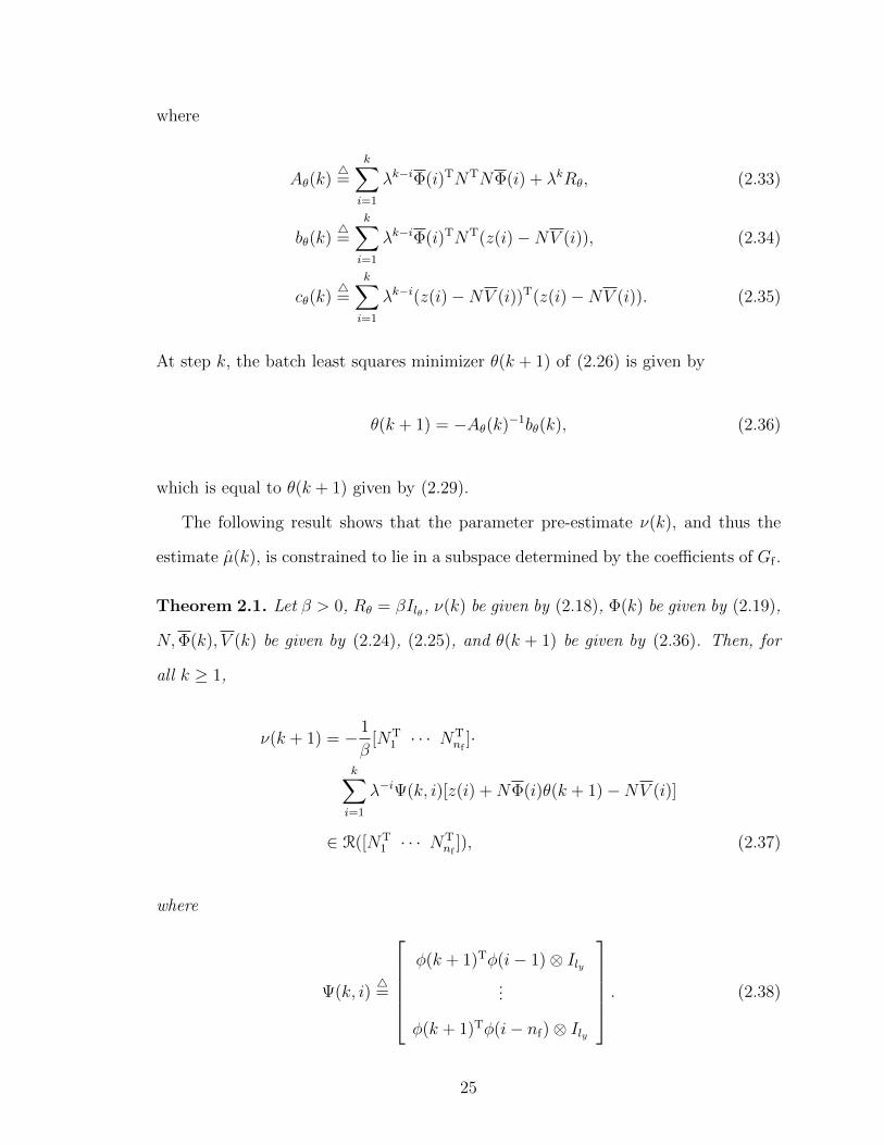
Theorem 2.1. Let β > 0, Rθ = βIlθ , ν(k) be given by (2.18), Φ(k) be given by (2.19),
N,Φ(k), V (k) be given by (2.24), (2.25), and θ(k + 1) be given by (2.36). Then, for
all k ≥ 1,
ν(k + 1) = − 1
β[NT
1 · · · NTnf
]·
k∑i=1
λ−iΨ(k, i)[z(i) +NΦ(i)θ(k + 1)−NV (i)]
∈ R([NT1 · · · NT
nf]), (2.37)
where
Ψ(k, i)4=
φ(k + 1)Tφ(i− 1)⊗ Ily
...
φ(k + 1)Tφ(i− nf)⊗ Ily
. (2.38)
25
Proof. Note that
Φ(k + 1)Aθ(k)θ(k + 1) =k∑i=1
λk−iΦ(k + 1)(Φ(i)TNTNΦ(i)
)θ(k + 1)+
λkβΦ(k + 1)θ(k + 1)
=k∑i=1
(λk−i
nf∑j=1
(Ilu ⊗ φ(k + 1)T)(Ilu ⊗ φ(i− j))NTj
)·
NΦ(i)θ(k + 1) + λkβΦ(k + 1)θ(k + 1)
=k∑i=1
(λk−i
nf∑j=1
NTj φ(k + 1)Tφ(i− j)
)NΦ(i)θ(k + 1)+
λkβΦ(k + 1)θ(k + 1)
= [NT1 · · · NT
nf]
k∑i=1
λk−iΨ(k, i)NΦ(i)θ(k + 1)+
λkβΦ(k + 1)θ(k + 1) (2.39)
and
Φ(k + 1)bθ(k) = Φ(k + 1)k∑i=1
λk−iΦ(i)TNT(z(i)−NV (i)
)= [NT
1 · · · NTnf
]k∑i=1
λk−iΨ(k, i)(z(i)−NV (i)
). (2.40)
Writing (2.36) as Aθ(k)θ(k + 1) = −bθ(k), multiplying by Φ(k + 1), and using (2.39)
and (2.40) yields (2.37).
It follows from Lemma 2.1 that the parameter pre-estimate ν is constrained to
lie in the subspace of Rlµ spanned by the coefficients of the filter used by RCPE. In
addition to the subspace constraint, the numerical examples in sections 2.5–2.8 show
that the feasible region is determined by the choice of the filter coefficients. The
feasible region is the set of parameter pre-estimates in Rlµ that are asymptotically
26

reachable by the estimator. Consequently, the permutation matrix Op must be chosen
such that at least one element of SOp , defined in (2.17), lies in the feasible region.
In view of Lemma 2.1, for all examples in this chapter where lz = 1, nf is set to be
equal to lµ, and each filter coefficient is chosen to be an element of {e1, e2, . . . , elµ},
where ei is the ith row of the identity matrix Ilµ . For lz > 1, the filter coefficients
must be selected such that µ ∈ R([NT1 · · · NT
nf]).
2.5 Examples with lµ = ly = 1
In this section, RCPE is used to estimate one parameter in an affinely and non-
affinely parameterized linear systems.
Example 2.1. Affinely parameterized linear dynamics with one unknown parameter
in the dynamics matrix. This example shows the effect of u , x(0) and N1 on the
feasible region. Consider the linear system (2.8), (2.9), where
A(µ) =
µ 0.2
0.1 0.6
, B =
0.9
0.3
, C =
[1.1 0.5
], (2.41)
and µ = 0.3. The initial state is x(0) = [10 10]T, the input is
u(k) = 2 +15∑j=1
sin
(2πj
100k
), (2.42)
N1 = 1, λ = 1, and Rθ = 106. Furthermore, O1 = 1, and thus S1 = {±µ}. Figure 2.3
shows the output error, true parameter, parameter pre-estimate, parameter estimate,
state-estimate error, and estimator coefficient. (b) shows that ν(k) converges to −µ,
and thus, by (2.16), µ(k) = |ν(k)| converges to µ. Unless stated otherwise, the
abscissa of all plots denotes the iteration step.
27

10-6
10-3
100
-0.2
0
0.2
100 200
10-6
10-3
100
100 200
-3
-2
-1
010
-3
Figure 2.3: Example 2.1. (a) output error, (b) true parameter, parameter pre-
estimate, and parameter estimate, (c) state-estimate error, (d) parameter
estimator coefficient.
In order to investigate the effect of u and N1 on the feasible region, µ is estimated
with the input αu, where u is given by (2.42), α = ±1, and N1 = ±1. For all four
cases, Figure 2.4 shows the true parameter, parameter pre-estimate, and parameter
estimate. Note that, for a given input u and filter coefficient N1, ν(k) converges to
either µ or −µ, and thus µ(k) converges to µ.
28

50 100 150 200 250
-0.2
0
0.2
(a) N1 = 1, α = 1.
50 100 150 200 250
0
0.1
0.2
0.3
(b) N1 = −1, α = 1.
50 100 150 200 250
0
0.1
0.2
0.3
(c) N1 = 1, α = −1.
50 100 150 200 250
-0.2
0
0.2
(d) N1 = −1, α = −1.
Figure 2.4: Example 2.1. Parameter pre-estimate ν(k) and the estimate µ(k) for
various choices of the filter coefficient N1 and the input u determined by
the parameter α.
Next, to investigate the effect of the initial conditions of (2.8), (2.9) on the perfor-
mance of RCPE, µ is estimated with x1(0) and x2(0) varied from −100 to 100. The
input u(k) is given by (2.42) in all cases. Each point in Figure 2.5 (a),(b) corresponds
to an initial condition of (2.8), (2.9), where green indicates that ν(k) converges to µ,
blue indicates that ν(k) converges to −µ, and red indicates that ν(k) diverges. Note
that all cases are obtained by running RCPE under the same values of λ and Rθ;
however, the set of initial conditions x(0) for which ν(k) converges can be expanded
by varying these parameters. Figures 2.4 and 2.5 suggest that, for the given input
29
u and filter coefficient N1, the feasible region is either (−∞, 0] or [0,∞), and thus
cannot be determined a priori. Consequently, (2.16) ensures that there exists s ∈ SOp
in the feasible region such that, ν(k) converges to s , and thus µ(k) converges to µ. �
-100 -50 0 50 100
-100
-50
0
50
100
(a) N1 = −1
-100 -50 0 50 100
-100
-50
0
50
100
(b) N1 = 1
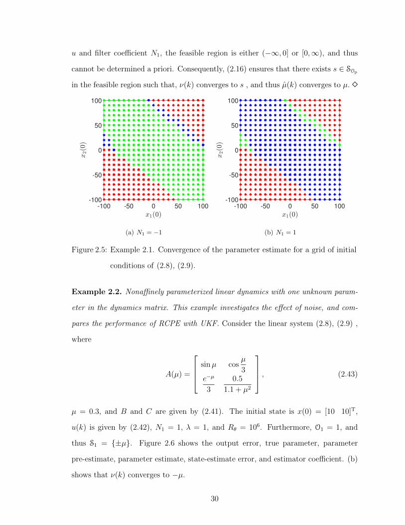
Figure 2.5: Example 2.1. Convergence of the parameter estimate for a grid of initial
conditions of (2.8), (2.9).
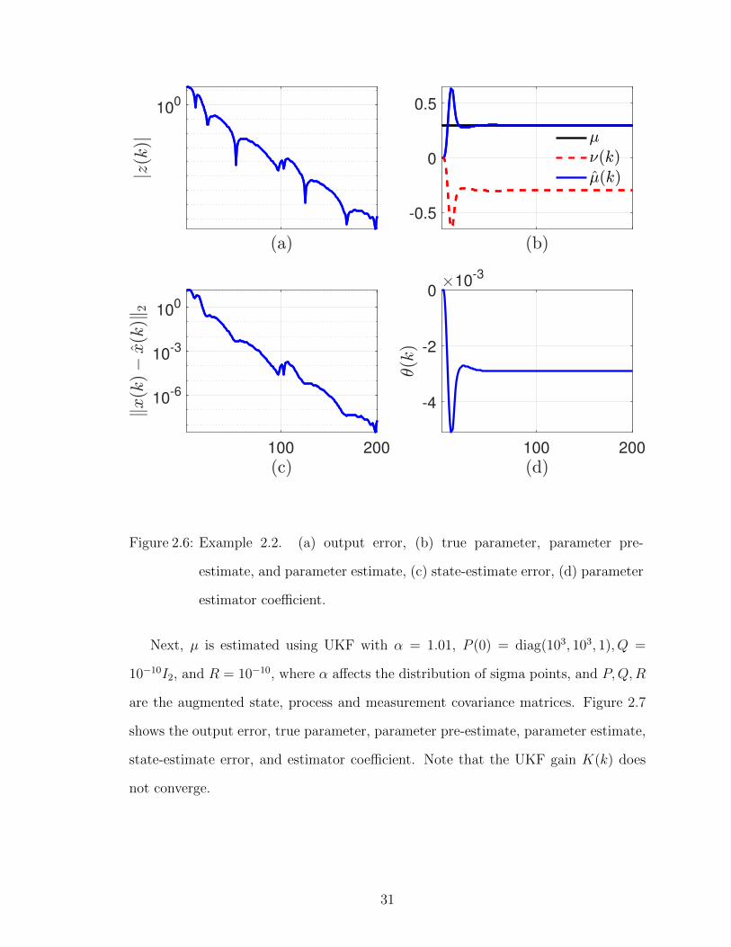
Example 2.2. Nonaffinely parameterized linear dynamics with one unknown param-
eter in the dynamics matrix. This example investigates the effect of noise, and com-
pares the performance of RCPE with UKF. Consider the linear system (2.8), (2.9) ,
where
A(µ) =
sinµ cosµ
3e−µ
3
0.5
1.1 + µ2
, (2.43)
µ = 0.3, and B and C are given by (2.41). The initial state is x(0) = [10 10]T,
u(k) is given by (2.42), N1 = 1, λ = 1, and Rθ = 106. Furthermore, O1 = 1, and
thus S1 = {±µ}. Figure 2.6 shows the output error, true parameter, parameter
pre-estimate, parameter estimate, state-estimate error, and estimator coefficient. (b)
shows that ν(k) converges to −µ.
30
100
-0.5
0
0.5
100 200
10-6
10-3
100
100 200
-4
-2
010
-3
Figure 2.6: Example 2.2. (a) output error, (b) true parameter, parameter pre-
estimate, and parameter estimate, (c) state-estimate error, (d) parameter
estimator coefficient.
Next, µ is estimated using UKF with α = 1.01, P (0) = diag(103, 103, 1), Q =
10−10I2, and R = 10−10, where α affects the distribution of sigma points, and P,Q,R
are the augmented state, process and measurement covariance matrices. Figure 2.7
shows the output error, true parameter, parameter pre-estimate, parameter estimate,
state-estimate error, and estimator coefficient. Note that the UKF gain K(k) does
not converge.
31

10-12
10-9
10-6
10-3
100
100 200
10-9
10-6
10-3
100
0
0.2
0.4
100 200
-1
0
1
Figure 2.7: Example 2.2. UKF-based parameter estimation. (a) output error, (b) true
parameter and parameter estimate, (c) state-estimate error, (d) compo-
nents of the UKF based estimator gain.
Next, to compare the accuracy of RCPE and UKF in the presence of noise,
µ is estimated with process noise w1 ∼ N(0, σ21I2) and measurement noise w2 ∼
N(0, σ22). For RCPE, N1 = 1, λ = 1, and Rθ = 106; for UKF, α = 1.01, P (0) =
diag(103, 103, 1), Q = σ1I2, and R = σ2. For a range of values of σ1 and σ2, Figure
2.8 shows
εµ4=
1
100
√√√√ 1000∑i=901
(µ(i)− µ)2. (2.44)
32

Note that, unlike UKF, RCPE uses no knowledge of the noise statistics Q and R to
compute µ. �
-10 -8 -6 -4 -2
-10
-8
-6
-4
-2
-11
-10
-9
-8
-7
-6
-5
-4
-3
(a) RCPE
-10 -8 -6 -4 -2
-10
-8
-6
-4
-2
-11
-10
-9
-8
-7
-6
-5
-4
-3
(b) UKF
Figure 2.8: Example 2.2. Effect of noise on the estimation accuracy of (a) RCPE and
(b) UKF; the color scale denotes values of log εµ as a function of σ1 and
σ2.
2.6 Example with lµ = ly = 2
In this section, RCPE is used to estimate two unknown parameters in linear
systems that are affinely and nonaffinely parameterized with two measurements.
Example 2.3. Nonaffinely parameterized linear dynamics with two measurements
and two unknown parameters. This example shows how RCPE can be implemented
with a sparse R(k). Consider the linear system (2.8), (2.9), where
A(µ) =
sinµ1 cos µ13
e−µ1
3
0.5
1.1 + µ21
, B(µ) =
log(1 + µ22)
1 + sinµ2
, C(µ) =
µ2 4µ21
sinµ1 2µ2
,(2.45)
33
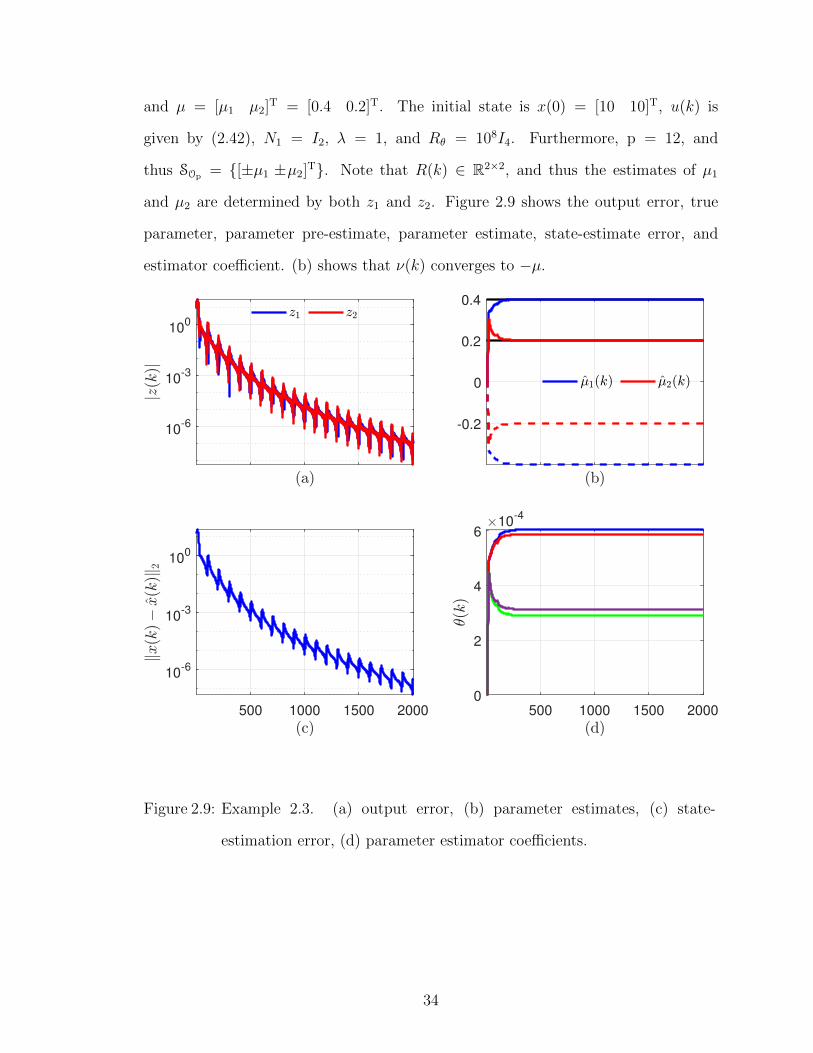
and µ = [µ1 µ2]T = [0.4 0.2]T. The initial state is x(0) = [10 10]T, u(k) is
given by (2.42), N1 = I2, λ = 1, and Rθ = 108I4. Furthermore, p = 12, and
thus SOp = {[±µ1 ±µ2]T}. Note that R(k) ∈ R2×2, and thus the estimates of µ1
and µ2 are determined by both z1 and z2. Figure 2.9 shows the output error, true
parameter, parameter pre-estimate, parameter estimate, state-estimate error, and
estimator coefficient. (b) shows that ν(k) converges to −µ.
10-6
10-3
100
-0.2
0
0.2
0.4
500 1000 1500 2000
10-6
10-3
100
500 1000 1500 2000
0
2
4
610
-4
Figure 2.9: Example 2.3. (a) output error, (b) parameter estimates, (c) state-
estimation error, (d) parameter estimator coefficients.
34
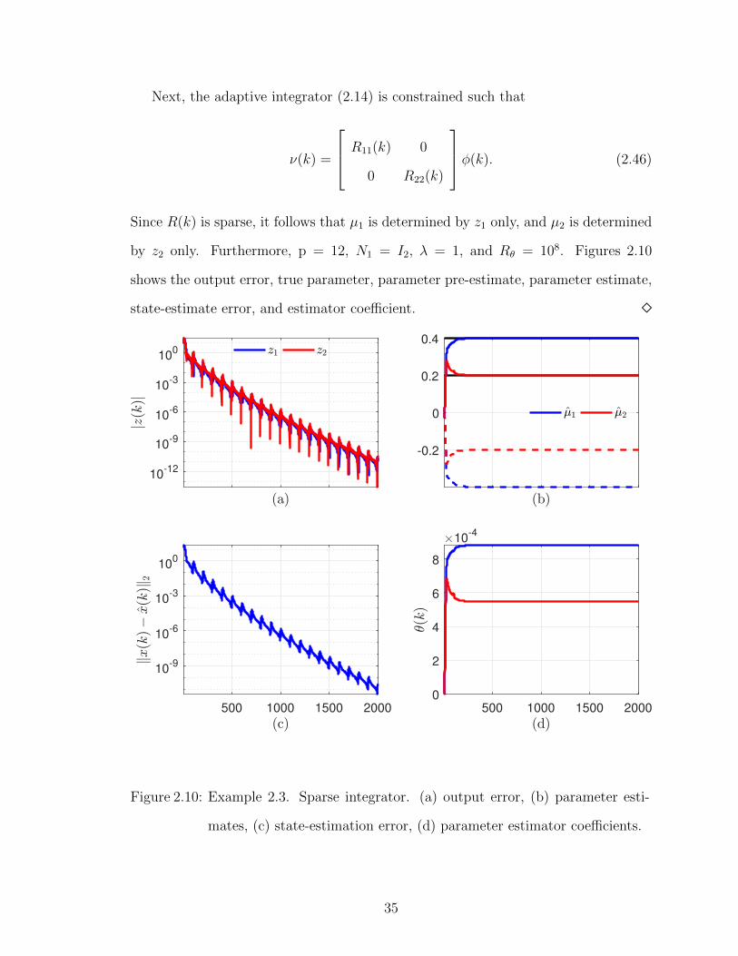
Next, the adaptive integrator (2.14) is constrained such that
ν(k) =
R11(k) 0
0 R22(k)
φ(k). (2.46)
Since R(k) is sparse, it follows that µ1 is determined by z1 only, and µ2 is determined
by z2 only. Furthermore, p = 12, N1 = I2, λ = 1, and Rθ = 108. Figures 2.10
shows the output error, true parameter, parameter pre-estimate, parameter estimate,
state-estimate error, and estimator coefficient. �
10-12
10-9
10-6
10-3
100
-0.2
0
0.2
0.4
500 1000 1500 2000
10-9
10-6
10-3
100
500 1000 1500 2000
0
2
4
6
8
10-4
Figure 2.10: Example 2.3. Sparse integrator. (a) output error, (b) parameter esti-
mates, (c) state-estimation error, (d) parameter estimator coefficients.
35

2.7 Examples with lµ = 2 and ly = 1
In this section, RCPE is used to estimate two unknown parameters in affinely and
nonaffinely parameterized systems with one measurement. These examples show that
the feasible region is determined by the choice and ordering of the filter coefficients.
Example 2.4. Affinely parameterized linear dynamics with two unknown parameters
in the dynamics matrix. This example investigates the effect of N1, N2, and Op on
the feasible region. Consider the linear system (2.8), (2.9), where
A(µ) =
µ1 µ2
0.1 0.6
, (2.47)
the input and output matrices are given by (2.41), and µ = [µ1 µ2]T = [0.3 0.2]T. The
initial state is x(0) = [10 10]T, u(k) is given by (2.42), N1 = e1, N2 = e2, λ = 0.999,
and Rθ = 106I2. Furthermore, p = 12, and thus SO12 = {[±µ1 ±µ2]T}. Figures 2.11
shows the output error, true parameter, parameter pre-estimate, parameter estimate,
state-estimate error, and estimator coefficient. (b) shows that ν(k) converges to −µ.
36

Figure 2.11: Example 2.4. (a) output error, (b) true parameter, parameter pre-
estimate, and parameter estimate, (c) state-estimate error, (d) parame-
ter estimator coefficients.
Next, the effect of the choice of Op and N1 and N2 is investigated. For lµ = 2,
there are two choices of Op and two ways to order the filter coefficients e1 and e2.
Further, for each ordering, there are four ways to allocate signs. Table 2.2 shows all
such filter choices. Figure 2.12(a) shows ν(k) for p = 12, and Figure 2.12(b) shows
ν(k) for p = 21, where the corresponding filter coefficients are given in Table 2.2. Note
that, for a fixed ordering of the filter coefficients, there is exactly one permutation
matrix Op such that the parameter pre-estimate ν converges to an element of SOp .
Conversely, for a fixed permutation matrix Op, there is exactly one ordering of the
37

filter coefficients such that the parameter pre-estimate ν converges to an element of
SOp . �
N1 N2
Gf1 e1 e2
Gf2 −e1 e2
Gf3 e1 −e2
Gf4 −e1 −e2
N1 N2
Gf5 e2 e1
Gf6 −e2 e1
Gf7 e2 −e1
Gf8 −e2 −e1
Table 2.2: Filter coefficients for Example 2.4.
-0.2 -0.1 0 0.1 0.2
-0.2
-0.1
0
0.1
0.2
(a) p = 12.
-0.2 -0.1 0 0.1 0.2
-0.2
-0.1
0
0.1
0.2
(b) p = 21.
Figure 2.12: Example 2.4. Parameter pre-estimate ν(k) for various choices of Gf given
in Table 2.2. The true parameter µ is shown in red.
Example 2.5. Nonaffinely parameterized nonlinear dynamics with two unknown pa-
rameters. This example investigates the effect of N1, N2, and Op on the feasible region.
38

Consider the (3,3) type nonlinear system [37, p. 183]
x(k + 1) =
x2(k)
1 + 0.8x2(k) + x1(k)
1 + µ1x2(k) + µ2x1(k)
+
0
1
u(k), (2.48)
y(k) = x1(k), (2.49)
where µ = [µ1 µ2]T = [0.6 1.1]T. The initial state is x(0) = [10 10]T, u(k) is given
by
u(k) = 2 +5∑j=1
1
jsin
(2πj
100k + j2
), (2.50)
N1 = e2, N2 = e1, λ = 0.999, and Rθ = 1012I2. Furthermore, p = 21, and thus
SOp = {[±µ2 ±µ1]T}. Figure 2.13 shows the output error, true parameter, parameter
pre-estimate, parameter estimate, state-estimate error, and estimator coefficient. (b)
shows that ν(k) converges to O−1p µ. Analogous results shown in Figure 2.12 are
obtained for other choices of the filter coefficients and permutation matrix Op.
Figure 2.14(a) shows ν(k) for p = 21, and Figure 2.14(b) shows ν(k) for p = 12,
where the corresponding filter coefficients are given in Table 2.2. Note that, for a fixed
ordering of the filter coefficients, there is exactly one permutation matrix Op such that
the parameter pre-estimate ν converges to an element of SOp . Conversely, for a fixed
permutation matrix Op, there is exactly one ordering of the filter coefficients such
that the parameter pre-estimate ν converges to an element of SOp . �
39

10-9
10-6
10-3
100
0
0.5
1
1 2 3
104
10-9
10-6
10-3
100
1 2 3
104
-10
-5
010
-5
Figure 2.13: Example 2.5. (a) output error, (b) true parameter, parameter pre-estimate, and parameter estimate, (c) state-estimate error, (d) parame-ter estimator coefficients.
40

-1 -0.5 0 0.5 1
-0.5
0
0.5
1
(a) p = 21.
-0.5 0 0.5
-1
-0.5
0
0.5
1
(b) p = 12.
Figure 2.14: Example 2.5. Parameter pre-estimate ν(k) for various choices of Gf given
in Table 2.2. The true parameter µ is shown in red.
2.8 Examples with lµ = 3 and ly = 1
In this section, RCPE is used to estimate three unknown parameters in affinely
and nonaffinely parameterized systems with one measurement.
Example 2.6. Affinely parameterized linear dynamics with three unknown parame-
ters in the dynamics matrix. This example investigates the effect of N1, N2, N3, and
Op on the feasible region. Consider the linear system (2.8), (2.9), where
A(µ) =
µ1 µ2
0.1 µ3
, (2.51)
the input and output matrices are given by (2.41), and µ = [µ1 µ2 µ3]T =
[0.3 0.2 0.6]T. The initial state is x(0) = [10 10 10]T, u(k) is given by (2.42),
N1 = e3, N2 = e2, N3 = e1, λ = 0.999, and Rθ = 106I2. Furthermore, p = 123, and
thus SOp = {[±µ1 ±µ2 ±µ3]T}. Figures 2.15 shows the output error, true parame-
41
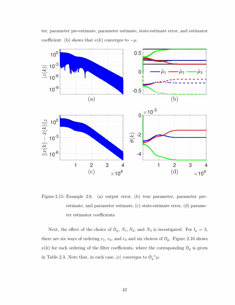
ter, parameter pre-estimate, parameter estimate, state-estimate error, and estimator
coefficient. (b) shows that ν(k) converges to −µ.
10-9
10-6
10-3
100
-0.5
0
0.5
1 2 3 4
104
10-6
10-3
100
1 2 3 4
104
-4
-2
010
-3
Figure 2.15: Example 2.6. (a) output error, (b) true parameter, parameter pre-
estimate, and parameter estimate, (c) state-estimate error, (d) parame-
ter estimator coefficients.
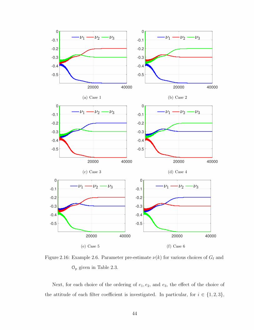
Next, the effect of the choice of Op, N1, N2, and N3 is investigated. For lµ = 3,
there are six ways of ordering e1, e2, and e3 and six choices of Op. Figure 2.16 shows
ν(k) for each ordering of the filter coefficients, where the corresponding Op is given
in Table 2.3. Note that, in each case, |ν| converges to O−1p µ.
42

Case N1 N2 N3 p
1 e1 e2 e3 321
2 e1 e3 e2 231
3 e2 e1 e3 312
4 e2 e3 e1 132
5 e3 e2 e1 123
6 e3 e1 e2 213
Table 2.3: Filter coefficients and Op for Example 2.6.
43
20000 40000
-0.5
-0.4
-0.3
-0.2
-0.1
0
(a) Case 1
20000 40000
-0.5
-0.4
-0.3
-0.2
-0.1
0
(b) Case 2
20000 40000
-0.5
-0.4
-0.3
-0.2
-0.1
0
(c) Case 3
20000 40000
-0.5
-0.4
-0.3
-0.2
-0.1
0
(d) Case 4
20000 40000
-0.5
-0.4
-0.3
-0.2
-0.1
0
(e) Case 5
20000 40000
-0.5
-0.4
-0.3
-0.2
-0.1
0
(f) Case 6
Figure 2.16: Example 2.6. Parameter pre-estimate ν(k) for various choices of Gf and
Op given in Table 2.3.
Next, for each choice of the ordering of e1, e2, and e3, the effect of the choice of
the attitude of each filter coefficient is investigated. In particular, for i ∈ {1, 2, 3},
44
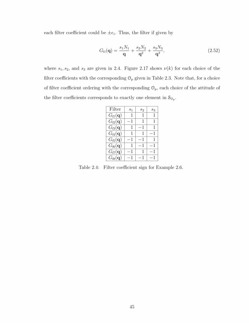
each filter coefficient could be ±ei. Thus, the filter if given by
Gfi(q) =s1N1
q+s2N2
q2+s3N3
q3, (2.52)
where s1, s2, and s3 are given in 2.4. Figure 2.17 shows ν(k) for each choice of the
filter coefficients with the corresponding Op given in Table 2.3. Note that, for a choice
of filter coefficient ordering with the corresponding Op, each choice of the attitude of
the filter coefficients corresponds to exactly one element in SOp .
Filter s1 s2 s3Gf1(q) 1 1 1Gf2(q) −1 1 1Gf3(q) 1 −1 1Gf4(q) 1 1 −1Gf5(q) −1 −1 1Gf6(q) 1 −1 −1Gf7(q) −1 1 −1Gf8(q) −1 −1 −1
Table 2.4: Filter coefficient sign for Example 2.6.
45
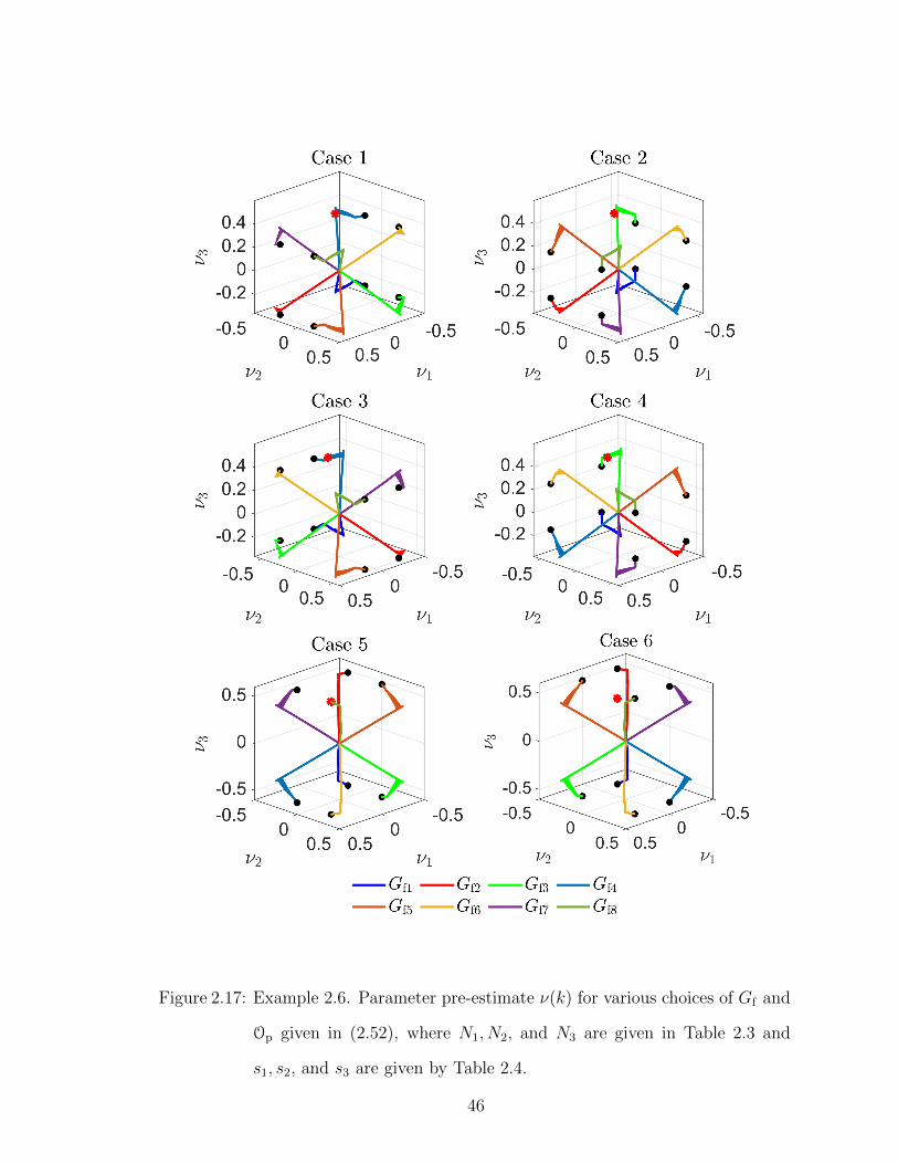
Figure 2.17: Example 2.6. Parameter pre-estimate ν(k) for various choices of Gf and
Op given in (2.52), where N1, N2, and N3 are given in Table 2.3 and
s1, s2, and s3 are given by Table 2.4.
46

�
Example 2.7. Affinely parameterized nonlinear dynamics with three unknown pa-
rameters. This example investigates the effect of N1, N2, N3, and Op on the feasible
region. Consider the (3,3) type nonlinear system [37, p. 183]
x(k + 1) =
x2(k)
µ1 + µ2x2(k) + µ3x1(k)
1 + 0.6x2(k) + 1.1x1(k)
+
0
1
u(k), (2.53)
y(k) = x1(k), (2.54)
where µ = [µ1 µ2 µ3]T = [0.5 0.8 1.0]T. The initial state is x(0) = [10 10 10]T,
u(k) is given by (2.42), N1 = e1, N2 = e2, N3 = e3, λ = 0.9999, and Rθ = 106I2.
Furthermore, p = 213, and thus SOp = {[±µ2 ±µ1 ±µ3]T}. Figures 2.18 shows
the output error, true parameter, parameter pre-estimate, parameter estimate, state-
estimate error, and estimator coefficient. Analogous results shown in Figure 2.16 are
obtained for other choices of the filter coefficients and the permutation matrix Op.
47

10-6
10-3
100
-0.5
0
0.5
1
0.5 1 1.5 2
105
10-6
10-3
100
0.5 1 1.5 2
105
-6
-4
-2
010
-3
Figure 2.18: Example 2.7. (a) output error, (b) true parameter, parameter pre-
estimate, and parameter estimate, (c) state-estimate error, (d) parame-
ter estimator coefficients.
Figure 2.19 shows the output error for all six permutations. For clarity, a subset
of the data is shown. Note that the output error diverges for all permutation but p =
213. Thus, diverging output error can be used to rule out the incorrect permutations.
48

0.2 0.4 0.6 0.8 1 1.2 1.4 1.6 1.8 2
105
10-6
10-4
10-2
100
321
312
231
213
132
123
Figure 2.19: Example 2.7. Output error for all six permutations. [For clarity, only
a subset of the data is plotted.] For five of the six permutations, the
parameter error diverges. However, the correct permutation 213 yields
convergence to the true parameters.
Next, for each choice of the ordering of e1, e2, and e3, the effect of the choice of
the attitude of each filter coefficient is investigated. Figure 2.20 shows ν(k) for each
choice of the filter coefficients with the corresponding Op given in Table 2.5. Note
that, for a choice of filter coefficient ordering with the corresponding Op, each choice
of the attitude of the filter coefficients corresponds to exactly one element in SOp .
49
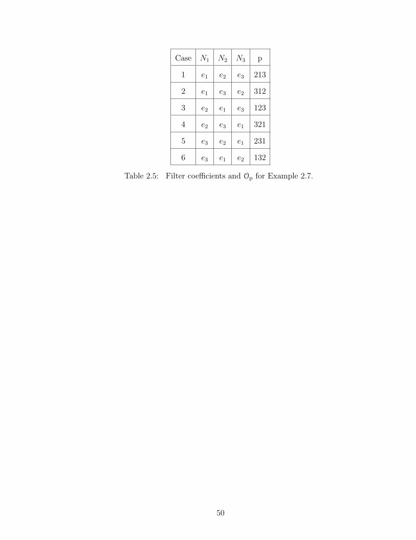
Case N1 N2 N3 p
1 e1 e2 e3 213
2 e1 e3 e2 312
3 e2 e1 e3 123
4 e2 e3 e1 321
5 e3 e2 e1 231
6 e3 e1 e2 132
Table 2.5: Filter coefficients and Op for Example 2.7.
50
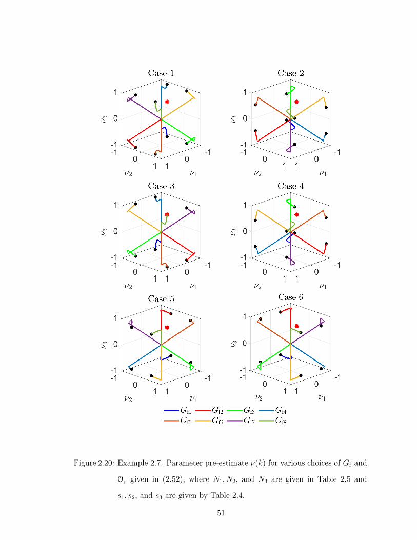
Figure 2.20: Example 2.7. Parameter pre-estimate ν(k) for various choices of Gf and
Op given in (2.52), where N1, N2, and N3 are given in Table 2.5 and
s1, s2, and s3 are given by Table 2.4.
51

�
2.9 Parameter Estimation in the Generalized Burgers Equa-
tion
In this section, we consider the generalized one-dimensional viscous Burgers equa-
tion [38]
∂u
∂t+ µ1
∂
∂x
u2
2=
∂
∂x
(µ2∂u
∂x
), (2.55)
where u(x, t) is a function of space and time with domain [0, 1]× [0,∞), µ1 > 0 is the
convective constant and µ2 > 0 is the viscosity. Note that there is no external input to
this system and u is used to denote the solution of this partial differential equation.
The initial condition is u(x, 0) = 0 for all x ∈ [0, 1], and the boundary conditions
are u(0, t) = 0 and u(1, t) = sin(5t) + 0.25 sin(10t) for all t ≥ 0. The objective is to
estimate the unknown parameter µ4= [µ1 µ1]
T using measurements of u at a single
location.
The Burgers equation (2.55) is discretized using a forward Euler approximation
for the time derivative, a second-order-accurate upwind method for the convective
term, and a second-order-accurate central difference scheme for the viscous term.
The spatial domain [0, 1] is discretized using N equally spaced grid points; thus
∆x4= 1
N−1 . The time step ∆t is chosen to satisfy the CFL condition, that is,
∆t <Cmax∆x
|max(u)|, (2.56)
where the Courant number Cmax depends on the discretization scheme [39]. Finally,
the discrete variable uj(k)4= u((j − 1)∆x, k∆t) is defined on the grid points j ∈
52

{1, . . . , N} for all time steps k ≥ 0. Hence, at each grid point, j ∈ {3, . . . , N − 1},
uj(k + 1) = uj(k)− µ1∆t
2∆x(1.5uj(k)2 − 2uj−1(k)2 + 0.5uj−2(k)2)+
µ2∆t
∆x2(uj+1(k)− 2uj(k) + uj−1(k)). (2.57)
For all k ≥ 0, the discretized boundary conditions are
u1(k) = u2(k) = 0, uN(k) = sin(5∆tk) + 0.25 sin(10∆tk), (2.58)
and, for all j ∈ {3, . . . , N − 1}, the initial condition is
uj(0) = 0. (2.59)
In this example, µ1 = 1.4, µ2 = 0.3, Cmax = 0.25, N = 100, and ∆t = 10−4 s.
Figure 2.21(a) shows the numerical solution of (2.57) with the boundary conditions
(2.58) and initial conditions (2.59), where the solid black line shows the measurement
location. Figure 2.21(b) shows the measurement y(k)4= u87(k) = u(0.87, k∆t).
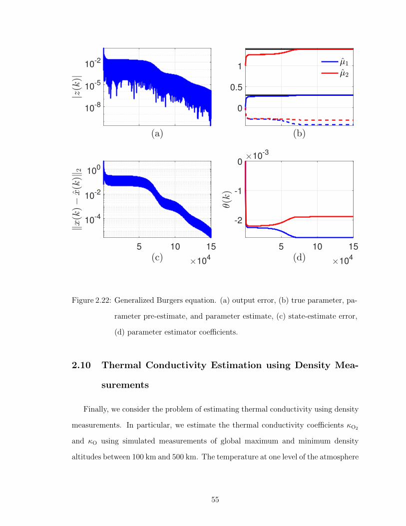
In order to start the estimation model, nonzero values of µ1(0) and µ2(0) are
needed. A simple way to ensure this is to replace µ by µ(k) = µ+Opν(k), where µ =
[µ1 µ1]T = [1 0.01]T, so that µ(0) 6= 0 . Furthermore, N1 = e1, N2 = e2, λ = 0.9999,
and Rθ = 106I2. Let p = 21 so that SOp = {[±(µ2 − µ2) ± (µ1 − µ2)]T}. Figure 2.22
shows the output error, true parameter, parameter pre-estimate, parameter estimate,
state-estimate error, and estimator coefficient.
53

(a) u(x, t)
2 4 6 8 10
-0.5
0
0.5
(b) y(t)
Figure 2.21: Simulation of the generalized Burgers equation with the discretization
(2.57).
54
10-8
10-5
10-2
0
0.5
1
5 10 15
104
10-4
10-2
100
5 10 15
104
-2
-1
010
-3
Figure 2.22: Generalized Burgers equation. (a) output error, (b) true parameter, pa-
rameter pre-estimate, and parameter estimate, (c) state-estimate error,
(d) parameter estimator coefficients.
2.10 Thermal Conductivity Estimation using Density Mea-
surements
Finally, we consider the problem of estimating thermal conductivity using density
measurements. In particular, we estimate the thermal conductivity coefficients κO2
and κO using simulated measurements of global maximum and minimum density
altitudes between 100 km and 500 km. The temperature at one level of the atmosphere
55

depends on the vertical structure of the temperature through the equation
δT
δt∝ δ
δzλδT
δz, (2.60)
where T is the temperature, t is time, z is altitude, and λ is approximated as
λ =κO2NO2 + κONO
NO2 +NO
T S, (2.61)
where the parameters κO2 and κO depend on the density of atomic (NO) and molecular
(NO2) oxygen, and S is independent of both.
To illustrate the application of RCPE to estimate thermal conductivity coeffi-
cients κO2 and κO, we generate measurements from a simulation of Global Ionosphere
Thermosphere Model (GITM), described in detail in Section 3.2, with thermal con-
ductivity coefficients κO2 = 0.00036 and κO = 0.00056. In particular, we record
minimum and maximum values of the density between 100 and 500 km.
In the estimation model, the thermal conductivity coefficients estimates are given
by
κO2(k)
κO(k)
=
κO2
κO
+ Op|ν(k)|, (2.62)
where κO2 = 0.00031 and κO = 0.00030 are the initial guesses of thermal conductivity
coefficients. In RCPE, we set N1 = I2, λ = 0.999, Rθ = 108I2, and p = 12. Figure 2.23
shows the output error, true parameter, parameter pre-estimate, parameter estimate,
estimated and measured densities, and the estimator coefficient.
56
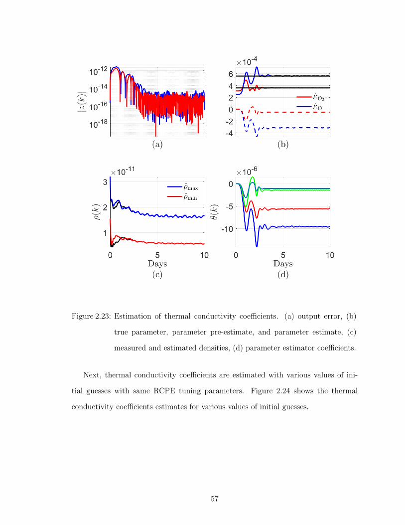
Figure 2.23: Estimation of thermal conductivity coefficients. (a) output error, (b)
true parameter, parameter pre-estimate, and parameter estimate, (c)
measured and estimated densities, (d) parameter estimator coefficients.
Next, thermal conductivity coefficients are estimated with various values of ini-
tial guesses with same RCPE tuning parameters. Figure 2.24 shows the thermal
conductivity coefficients estimates for various values of initial guesses.
57
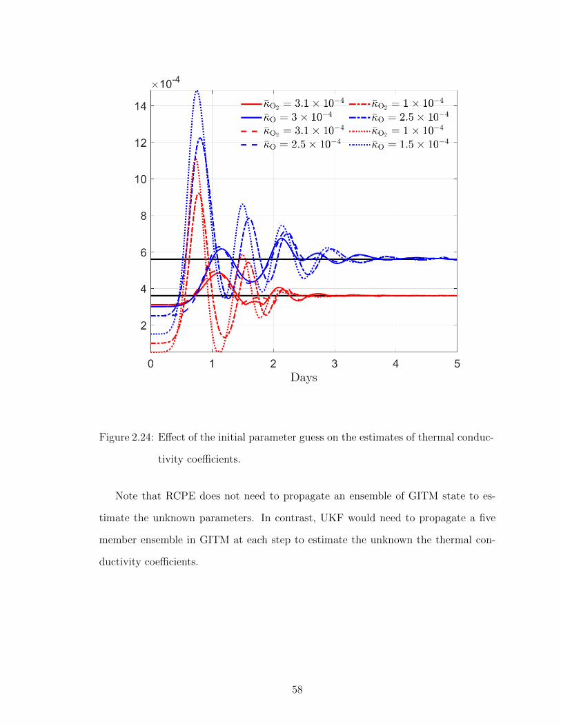
Figure 2.24: Effect of the initial parameter guess on the estimates of thermal conduc-
tivity coefficients.
Note that RCPE does not need to propagate an ensemble of GITM state to es-
timate the unknown parameters. In contrast, UKF would need to propagate a five
member ensemble in GITM at each step to estimate the unknown the thermal con-
ductivity coefficients.
58

2.11 Conclusions
This chapter presented RCPE, which is an iterative, data-driven technique for
estimating unknown parameters in linear and nonlinear dynamical systems. Unlike
the extended Kalman filter, RCPE is gradient-free; unlike the unscented Kalman
filter, RCPE is ensemble-free; and unlike variational methods, RCPE is adjoint-free.
It is shown that to estimate multiple unknown parameters, a permutation matrix
is required to correctly associate each parameter estimate with the corresponding
unknown parameter. The need to select the permutation matrix is the price paid
for not requiring gradient information, an ensemble of models, or an adjoint model.
The potential usefulness of RCPE was demonstrated by application to the Burgers
equation and GITM. In the Burgers equation, UKF requires an ensemble of 207
models each with 101 states, requiring a total of 21,321 state updates. In contrast,
RCPE required one model and testing of two permutations, which requires a total
of 202 state updates (101 for each permutation). In GITM which has ∼ 106 states,
in the case where UKF is applied to update the unknown parameters only, a five
member ensemble needs to be propagated at each step to estimate the unknown the
thermal conductivity coefficients, increasing the computational cost by at least five
times. In contrast, RCPE required a single propagation of GITM states and testing
of two permutations.
In the next chapter, RCPE is extended to the case where the filter coefficients that
define the retrospective cost are simultaneously optimized along with the parameter
estimator coefficient. The extended RCPE is applied to the problem of estimating
eddy diffusion coefficient in GITM using the measurements of total electron content.
59
CHAPTER 3
Estimation of the Eddy Diffusion Coefficient Using
Total Electron Content Data
3.1 Introduction
Computational models of high-dimensional complex physical systems often have
unknown parameters. These parameters might be unknown due to lack of a physical
measurement equipment. For example, measurements of friction force to estimate
friction coefficients might not be available. In addition, the unknown parameters
might be used as a proxy for the cumulative effect of a complex phenomenon, and thus
are representational nature, that is, they may not have a true value. For example, the
subgrid stresses in large eddy simulations are modeled using constitutive relationships
using unknown coefficients.
The present chapter focuses on estimation of such uncertain parameters arising
in a model of the upper atmosphere, which extends from about 60 km to 1000 km.
The basis of this model is the Navier-Stokes equations coupled with electrodynamics
equations. The source terms driving the ionosphere, such as the solar flux and the
Earth’s magnetic field, as well as coupling effects such as viscosity and diffusion,
are constructed statistically [40] or empirically to match the predicted output of the
model with measurements from various ground stations and satellites in orbit.
60

It is well known that turbulent diffusion affects energy deposition and transport
of chemical species in the upper atmosphere. Eddy diffusion coefficient (EDC) is
used to model this mixing process. Specifically, EDC models turbulent mixing in the
upper atmosphere [41]. According to mass continuity and the momentum equations,
the altitude profile of the neutral constituents changes from full mixing at lower
altitudes (below 150 km), where turbulent mixing prevails, to molecular diffusion
at higher altitudes (above 150 km). The value of EDC represents the intensity of
the turbulent mixing, which is a key factor in determining the free-electron density
in the ionosphere, usually measured by total electron content (TEC). However, no
measurement device can directly measure EDC, and no first-principles physics model
is available to determine its value. Nevertheless, models of the upper atmosphere
routinely simulate the turbulent mixing at various altitudes by using shape functions
parameterized by EDC [42].
The estimates of EDC obtained in the present chapter are based on measurements
of the total electron content (TEC). TEC, defined as the total number of electrons
integrated along a vertical column of one meter squared cross section, is a widely used
quantity to describe the ionosphere. TEC is measured in TEC unit (TECU), where
1 TECU = 1016 electrons/m2. The free electrons in the ionosphere cause delay in the
propagation of radio waves in the atmosphere. Ionospheric irregularities also cause
random amplitude and phase fluctuations in the signals [43]. TEC measurements are
thus used to correct positioning errors and improve the accuracy of the Global Nav-
igation Satellite Systems [44]. Consequently, the physics of TEC are widely studied
[45–48]. TEC is routinely used to estimate the state of the ionosphere and thermo-
sphere [49–51]. The use of TEC measurements to estimate EDC is a novel element
of the present chapter.
In this chapter, we use retrospective cost parameter estimation (RCPE) to the
problem of estimating EDC. RCPE was applied to atmospheric models in [27, 52–54].
61

The present chapter extends RCPE by simultaneously optimizing the filter Gf ,
which is used to define the retrospective cost function [55, 56]. Within the context
of adaptive control, Gf is chosen to capture knowledge of the leading sign, relative
degree, and nonminimum-phase zeros. For parameter estimation within the context
of a high-order nonlinear model such as the atmospheric model considered in this
chapter, there are no clear guidelines for constructing Gf . Consequently, the present
chapter updates Gf online through a combined optimization procedure. A related
optimization technique within the context of adaptive control was considered in [57,
58].
The optimization problem involving both the unknown parameters and the filter
Gf turns out to be biquadratic. Although this biquadratic function is strictly convex
in each variable separately, it is highly nonconvex as a joint function of its arguments.
Unfortunately, numerical algorithms that converge globally to the global minimizer
of biquadratic functions are not available [59], and this poses a technical challenge
within the context of parameter estimation for large-scale physics models. In the
present chapter we apply an alternating convex search method that is guaranteed to
converge to a local minimizer.
The chapter is organized as follows. In Section 3.2, we describe GITM and the role
played by EDC. In Section 3.3, we summarize the RCPE algorithm. In section 3.4,
an algorithm to optimize the biquadratic retrospective cost function is presented. A
low-dimensional system illustrating the application of RCPE is presented in Section
3.5. Estimation of EDC using TEC is presented in 3.6. Finally, in Section 3.7, we
summarize the results of the chapter and discuss future directions.
3.2 Global Ionosphere-Thermosphere Model
GITM is a computational code that models the thermosphere and the ionosphere
of the Earth as well as that of various planets and moons by solving coupled continuity,
62

momentum, and energy equations [60]. By propagating the governing equations,
GITM computes neutral, ion, and electron temperatures, neutral-wind and plasma
velocities, and mass and number densities of neutrals, ions, and electrons. GITM uses
a uniform grid in latitude with width 2πnlat
rad, where nlat is the number of grid points.
In longitude and altitude, GITM uses a stretched grid to account for temperature
and density variations.
GITM is implemented in parallel, where the computational domain (the atmo-
sphere from 100 km to 600 km) is divided into blocks. Ghost cells border the physical
blocks to exchange information. GITM can be run in one-dimensional mode, where
horizontal transport is ignored, or in global three-dimensional mode. Furthermore,
GITM can be run at either a constant or a variable time step, which is calculated
by GITM based on the physical state and the user-defined CFL number in order
to maintain numerical stability. To initialize GITM, neutral and ion densities and
temperatures for a chosen time are set using the Mass Spectrometer and Incoherent
Scatter radar (MSIS) model [61] and International Reference Ionosphere (IRI) [62].
The model inputs for GITM are 10.7 cm solar radio flux (F10.7 index), hemispheric
power index (HPI), interplanetary magnetic field (IMF), solar wind plasma (SWP),
and solar irradiance, all of which are read from a text file containing the time of
measurements and the measured values. These signals are available from various
terrestrial sensor platforms.
3.3 Retrospective Cost Parameter Estimation
Consider the parameter estimator where the parameter pre-estimate ν is given by
µ(k) =lw∑i=1
Piν(k − i) +lw∑i=1
Qiz(k − i) +R(k)γ(k), (3.1)
63

where lw is the data-window length, and the integrator state γ(k) ∈ Rly is updated
by
γ(k) = γ(k − 1) + z(k − 1), (3.2)
and Pi(k) ∈ Rlµ×lµ , Qi(k), R(k) ∈ Rlµ×ly are the coefficient matrices, which are
updated by the RCPE algorithm. Finally, the parameter estimate µ(k) is given by
µ(k) = Op|ν(k)|, (3.3)
where Op is a permutation matrix described in Section 3.3.
We rewrite (3.1) as
ν(k) = Φ(k)θ(k), (3.4)
where the regressor matrix Φ(k) is defined by
Φ(k)4= Ilµ ⊗ φT(k) ∈ Rlµ×lθ ,
where
φ(k)4=
ν(k − 1)
...
ν(k − lw)
z(k − 1)
...
z(k − lw)
g(k)
, (3.5)
64

θ(k)4= vec
[P1(k) · · ·Plw(k) Q1(k) · · ·Qlw(k) R(k)
]∈ Rlθ , (3.6)
lθ4= l2µlw+lµly(lw+1), “⊗” is the Kronecker product, and “vec” is the column-stacking
operator.
3.3.1 Retrospective Cost Optimization
The retrospective error variable is defined by
z(k, θ, N) = z(k) + Gf(q)(Φ(k)θ − ν(k)), (3.7)
where θ ∈ Rlθ contains the parameter estimator coefficients to be optimized, and Gf
is an FIR filter of order nf to be optimized, given by
Gf(q) =
nf∑i=1
1
qiNi, (3.8)
where Ni ∈ Rly×lµ are the filter coefficients to be optimized. The retrospective error
variable (3.7) can thus be written as
z(k, θ, N) = z(k) + NΦ(k)θ − NV (k), (3.9)
where
N4=
[N1 · · · Nnf
]∈ Rly×nf lµ , (3.10)
and Φ(k) and V (k) are defined by (2.25).
Using the retrospective error variable z(k, θ, N), the retrospective cost function is
65
defined by
J(k, θ, N)4=
k∑i=1
λk−iz(k, θ, N)TRz z(k, θ, N) + λkθTRθθ, (3.11)
where Rz ∈ Rly×ly and Rθ ∈ Rlθ×lθ are positive definite, and λ ∈ (0, 1] is the forgetting
factor. Note that the retrospective cost J(k, θ, N) is a biquadratic function, that is,
J(k, θ, N) is a quadratic function of θ for fixed N , and a quadratic function of N
for fixed θ. We use alternating convex search (ACS) described in [59] to optimize the
retrospective cost with respect to the parameter estimator coefficients and the filter.
The parameter pre-estimate is given by
ν(k + 1) = Φ(k + 1)θ(k + 1), (3.12)
where θ(k + 1) is the minimizer of J(k, θ, N) at the kth step. Finally, the parameter
estimate at step k + 1 is given by
µ(k + 1) = Op|ν(k + 1)| = Op|Φ(k + 1)θ(k + 1)|. (3.13)
3.4 Biquadratic Retrospective Cost Optimization
In this section we show that J(k, θ, N) defined by (3.11) is biquadratic as a joint
function of the arguments θ and N and strictly convex in θ and N separately. This
property suggests an optimization algorithm in which J(k, θ, N) is minimized alter-
nately with respect to θ and N
66

3.4.1 Retrospective cost as a quadratic function of θ
We write the retrospective cost function (3.11) as
J(k, θ, N) = θTAθ(k, N)θ + θTbθ(k, N) + bθ(k, N)Tθ + cθ(k, N), (3.14)
where
Aθ(k, N)4=
k∑i=1
λk−iΦ(i)TNTNΦ(i) + λkRθ ∈ Rlθ×lθ , (3.15)
bθ(k, N)4=
k∑i=1
λk−i(NΦ(i)
)T(z(i)− NV (i)
)∈ Rlθ , (3.16)
cθ(k, N)4=
k∑i=1
λk−i[V (i)TNTNV (i) + z(i)Tz(i) + V (i)TNTz(i)] ∈ R. (3.17)
For fixed N , the global minimizer θ∗(k, N) of (3.11) is given by
θ∗(k, N) = −Aθ(k, N)−1bθ(k, N). (3.18)
3.4.2 Retrospective cost as a quadratic function of N
We write the retrospective cost function (3.11) as
J(k, θ, N)4= tr
(NAN(k, θ)NT + NBN(k, θ)T +BN(k, θ)NT + CN(k, θ)
), (3.19)
67

where
AN(k, θ)4=
k∑i=1
λk−i(Φ(i)θ − V (i)
)(Φ(i)θ − V (i)
)T ∈ Rnf lµ×nf lµ , (3.20)
BN(k, θ)4=
k∑i=1
λk−iz(i)(Φ(i)θ − V (i)
)T ∈ Rly×nf lµ , (3.21)
CN(k, θ)4=
k∑i=1
λk−iz(i)z(i)T ∈ Rly×ly . (3.22)
For fixed θ, the global minimizer N∗(k, θ) of (3.11) is given by
N∗(k, θ)4= −BN(k, θ)AN(k, θ)−T ∈ Rly×nf lµ . (3.23)
It follows from Theorem 2.1 that the pre-estimate ν(k) is constrained to lie in a
subspace defined by the coefficients of Gf(q). In particular, for all k ≥ 1, ν(k) ∈
R([NT1 · · · NT
nf]). Consequently, the filter order nf should be chosen such that
R([NT1 · · · NT
nf]) = Rlµ . (3.24)
For example, to estimate lµ unknown parameters with one measurement, nf should
be at least lµ.
3.4.2.1 Sparse Filter
The following result, given in [63], allows the construction of sparse filter coeffi-
cients.
Proposition 3.1. Let N be a sparse matrix with p nonzero entries. Let q be the
number of rows of N where the p nonzero entries appear; and let r be the number of
rows of N where the p nonzero entries appear. Then N can be written as E1NE2,
where E1 and E2 are matrices containing zero and one, and N contains the p nonzero
68

entries, if and only if p = qr.
In the case where ly = 1, we set nf = lµ, and constrain the filter coefficients Ni
to lie along the canonical basis vectors. In particular, it follows from Proposition 3.1
that N can be written as N = nE2. For example, let lµ = 2 and N = [n1e2 n2e1].
Then,
n =
[n1 n2
], (3.25)
E2 =
e2 0
0 e1
. (3.26)
In cases where it is not possible to write N = E1NE2, it is possible to set certain
components of the filter coefficients as constants, so that Proposition 3.1 can be used.
In such cases, N can be written as
N = E1nE2 + E0, (3.27)
where E0 contains the constants. For example,
N =
n1 0 n2 0
0 1 0 1
(3.28)
= E1
[n1 n2
]E2 + E0, (3.29)
where
E04=
0 0 0 0
0 1 0 1
, E14=
1
0
, E24=
1 0 0 0
0 0 1 0
. (3.30)
69

Finally, with sparse filter, the retrospective cost function (3.11) can be written as
J(k, θ, n)4= tr
(E1nAN(k, θ)nTET
1 + E1nBN(k, θ)T +BN(k, θ)nTET1 + CN(k, θ)
),
(3.31)
where
AN(k, θ) = E2AN(k, θ)ET2 , (3.32)
BN(k, θ) = E2BN(k, θ) + E2AN(k, θ)ET0 , (3.33)
CN(k, θ) = CN(k, θ) + E0AN(k, θ)ET0 + E0BN(k, θ) +BN(k, θ)TET
0 (3.34)
where AN(k, θ) is given by (3.20), BN(k, θ) is given by (3.21), and CN(k, θ) is given
by (3.22). For fixed θ, the global minimizer n∗(k, θ) of (3.31) is given by
n∗(k, θ)4= −(ET
1 E1)−1ET
1 BN(k, θ)AN(k, θ)−T. (3.35)
3.4.3 Alternating Convex Search algorithm
The ACS algorithm consists of using (3.23) and (3.18) alternately to converge to
a stationary point of (3.11). At step k, ACS consists of the following rules:
1. Set i = 0 and choose nonzero N0.
2. Use (3.18) with Ni to compute θi+1.
3. Use (3.23) with θi+1 to compute Ni+1.
4. Compute Ji+1(k, θi+1, Ni+1) using either (3.14) or (3.19).
5. For i > 2, if Ji+1 − Ji ≤ ε, then stop, where ε > 0 is the user-defined stopping
criteria, and set θ(k + 1) = θi+1 and N(k + 1) = Ni+1. Otherwise, replace i by
i+ 1 and go to 2).
70

Finally, the parameter pre-estimate is given by
ν(k + 1) = Φ(k + 1)θ(k). (3.36)
3.5 Illustrative example
In this section, RCPE is used to estimate an unknown scalar parameter µ that
nonaffinely parameterizes a linear system realization. Consider the LTI physical sys-
tem model
x(k + 1) = A(µ)x(k) +B(µ)u(k) + w1(k), (3.37)
y(k) = C(µ)x(k) + w2(k), (3.38)
where
A(µ) =
e−µ 1− µ
µ2 log(1 + µ2)
, (3.39)
B(µ) =
sinµ
1 + cosµ
, (3.40)
C(µ) =
[1 + µ µ2
]. (3.41)
The true value of µ is 0.8. The estimation model is thus
x(k + 1) = A(µ(k))x(k) +B(µ(k))u(k), (3.42)
y(k) = E(µ(k))x(k), (3.43)
where µ(k) is the output of the parameter estimator (3.1), (3.3) updated by RCPE.
The measurement y(k) is generated using the input u(k) = 2 + sin(2π40k)
+
71

sin(2π80k − 0.3
)+ sin
(2π160k − 0.5
), the initial state x(0) = [10 10]T, each component
of the process noise w1 is N(0, 10−6), and the measurement noise w2 is N(0, 10−6).
To reflect the absence of additional information, the initial state x(0) of the estima-
tion model and the initial estimate µ(0) of the unknown parameter µ are set to zero.
We use RCPE to estimate the unknown parameter µ in the linear system (3.37),
(3.38) with the nonlinear parameter dependence (3.39)-(3.41). We set lw = 1, nf = 1,
Rz = 1, and Rθ = 106Ilθ . At each step, ACS is initialized with N0 = −1. Figure 3.1
shows the estimate µ(k) of µ.
72

100 200 300
-20
0
20
(a)
100 200 300
0
0.2
0.4
0.6
0.8
(b)
50 100 150 200 250 300
0
1
2
3
(c)
100 200 300
0
0.02
0.04
(d)
100 200 300
0
20
40
(e)
100 200 300
-30
-25
-20
(f)
Figure 3.1: RCPE estimate of the unknown parameter µ in the linear system (3.37),
(3.38) with the nonlinear parameter dependence (3.39)-(3.41). (a) shows
the performance z on a linear scale, (b) shows the parameter estimate
µ, (c) shows the measured input u to the system, (d) shows the adapted
coefficients θ of the parameter estimator, (e) shows the measured out-
put and the output of the estimation model, and (f) shows the adapted
coefficient N(k) of the filter Gf .
73

Next, we investigate the effect of the ACS filter initialization N0 and the weight
Rθ on the performance of RCPE. We set lw = 1, nf = 1, and Rz = 1. Figure 3.2
shows the estimate µ(k) of µ and the filter coefficient N(k) for various initializations
and weights. Note that RCPE successfully estimates the unknown parameter µ for
ACS filter initialization choices ranging several orders of magnitude, thus indicating
that ACS filter initialization choice is not critical.
50 100 150 200 250
0
0.2
0.4
0.6
0.8
(a)
50 100 150 200 250
-30
-25
-20
(b)
50 100 150 200 250
0
0.5
1
(c)
50 100 150 200 250
-230
-220
-210
(d)
Figure 3.2: Effect of the ACS filter initialization N0 and the weight Rθ on the perfor-
mance of RCPE. (a) and (c) show the parameter estimate µ for various
values of the filter initialization N0 and the weight Rθ. (b) and (d) show
the filter coefficient N for various values of the filter initialization N0 and
the weight Rθ.
74

3.6 Estimation of EDC using TEC GITM
Finally, we consider the problem of estimating the EDC in the global ionosphere
thermosphere model (GITM) using measurements of TEC at a fixed ground station
on Earth.
To generate the measurements of TEC, we simulate the upper atmosphere of Earth
using GITM for the period starting at 00:00:00, 21-Nov-2002 and ending at 00:00:00,
8-Dec-2002 with EDC = 1750. TEC is computed at every minute at a fictitious
ground station located at 1 deg North, 45 deg East. The initial state of the upper
atmosphere, comprising neutral and ion densities and temperature, is set using MSIS
and IRI for the chosen start time. The inputs to GITM, such as F10.7 index, IMF
data, SWP data, and HPI data, are read from text files.
To estimate the unknown EDC, we compute the TEC at every minute at the
ground location 1 deg North, 45 deg East for the period starting from 00:00:00,
21-Nov-2002 to 00:00:00, 8-Dec-2002. The initial state of the upper atmosphere,
comprising neutral and ion densities and temperature, is set using MSIS and IRI for
the chosen start time. GITM is run for one simulation day, that is from 00:00:00,
21-Nov-2002 to 00:00:00, 22-Nov-2002 with EDC = 1500. At the start of the second
simulation day, RCPE is switched on. Note that the delayed starting of RCPE en-
sures that, at the instant RCPE starts, the state of the atmosphere updated by the
estimation GITM model is the not same as the GITM model used to generate the
TEC measurements.
We set lw = 2, nf = 1, Rz = 1, and Rθ = 10−1Ilθ , and use RCPE to update
the estimate of EDC at every minute. Figure 3.3 shows the estimate of EDC using
RCPE. Figure 3.4 shows the measured and computed TEC.
75

5 10 15
-8
-6
-4
-2
0
(a)
5 10 15
1500
2000
2500
3000
(b)
5 10 15
-10
-5
0
10-3
(c)
5 10 15
0
20
40
(d)
Figure 3.3: RCPE estimate of the unknown EDC in GITM. (a) shows the performance
z on a linear scale, (b) shows the EDC estimate, (c) shows the adapted
coefficient N(k) of the filter Gf , and (d) shows the adapted coefficients θ
of the parameter estimator.
76

Figure 3.4: Measured and computed TEC at the fictitious ground station located at 1
deg North, 45 deg East. y denotes the TEC measurements generated using
GITM with a constant EDC= 1750, and y denotes the TEC computed
by GITM where EDC is updated at every minute by RCPE.
Note that RCPE does not use GITM to update the parameter estimator. Instead,
GITM is used as a black box model, although the EDC estimate is injected into
GITM as a gray box model. In fact, the internal parameter dependence of GITM on
EDC is extremely complicated; fortunately, there is no need to explicitly characterize
this dependence.
77

3.7 Conclusions
This chapter presented an extension of retrospective cost parameter estimation
(RCPE) by concurrently optimizing the filter Gf and the parameter estimator. This
technique was used to estimate an unknown parameter in a large-scale model of
a physical system, namely, the eddy diffusion coefficient in the global ionosphere-
thermosphere model.
Analysis of RCPE focused on the biquadratic nature of the retrospective cost
function. Alternating convex search algorithm was used to optimize the biquadratic
retrospective cost function.
78
CHAPTER 4
Recursive Least Squares with Information-Driven
Directional Forgetting
Within the context of system identification, persistent excitation is crucial for
constructing estimators that converge to the unknown parameters. This convergence
depends on two things, namely, identifiability [64], which is ability to distinguish
distinct parameters, and persistent excitation, which refers to the spectral content
of the signals needed to ensure convergence of the parameter estimates to the true
parameter values [35, 65, 66]. Roughly speaking, the level of persistency must be
commensurate with the number of unknown parameters. For example, a harmonic
input has two-dimensional persistency and thus can be used to identify two parame-
ters, whereas white noise is sufficiently persistent for identifying an arbitrary number
of parameters. Within the context of adaptive control, persistent excitation is needed
to avoid bursting [67]; recent research has focused on relaxing these requirements
[68–70].
Under persistent excitation, a key issue in practice is the speed of convergence,
especially under changing conditions. For example, the parameters of a system may
change abruptly, and the goal is to ensure fast convergence to the modified param-
eters. The speed of convergence depends on the ability to forget past parameters
and incorporate new information. Although somewhat counterintuitive, the ability
79
to accommodate new information depends on the ability to forget. The ability to
forget is thus crucial to the ability to learn. This paradox is widely recognized, and
effective forgetting is of intense interest in machine learning [71].
This chapter considers forgetting within the context of recursive least squares
(RLS). In the classical RLS formulation, a constant forgetting factor λ ∈ (0, 1] can be
set by the user. However, it often occurs in practice that if λ is too small—perhaps as
small as 0.99—then RLS may diverge. This phenomenon has been extensively studied
and various remedies have been studied in the form of variable-rate forgetting [72–78].
The present chapter considers a technique that complements variable-rate forget-
ting, namely, directional forgetting. Directional forgetting has been widely studied
within the context of recursive least squares [79–85]. In the absence of persistent
excitation, new information is confined to a limited number of directions. The goal
of directional forgetting is thus to determine these directions and thereby constrain
forgetting to the directions in which new information is available. This technique
allows RLS to operate without divergence during periods of loss of persistency.
The chapter is organized as follows. Section 4.1 presents the classical recursive
least squares algorithm with constant scalar forgetting factor. Section 4.2 defines
persistency of excitation and presents results on bounds of the estimator variables.
Section 4.3 connects persistency of excitation of a sequence to the condition number
of the information matrix. Section 4.4 presents Lyapunov analysis of the parameter
error. Section 4.5 shows the effect of lack of persistent excitation on the estimator.
Section 4.6 introduces the information subspace, and Section 4.7 introduces the ma-
trix forgetting that constrains forgetting to the information directions receiving new
information. Finally, the chapter concludes in Section 4.8.
Table 4.1 summarizes the results and examples in this chapter.
80

Definition 4.1 Persistently exciting regressor
Definition 4.2 Uniformly Lyapunov stable equilibrium
Definition 4.3 Uniformly globally aymptotically stable equilibrium
Definition 4.4 Uniformly globally geometrically stable equilibrium
Theorem 4.1 Recursive least squares (RLS)
Theorem 4.2 Lyapunov stability theorem
Theorem 4.3 Lyapunov analysis of RLS for λ ∈ (0, 1)
Theorem 4.4 Stability analysis of RLS for λ ∈ (0, 1] based on θk
Proposition 4.1 Convergence of zk and θk
Proposition 4.2 Data-dependent subspace constraint on θk
Proposition 4.3 Bounds on Pk for λ = 1
Proposition 4.4 Bounds on Pk for λ ∈ (0, 1)
Proposition 4.5 Converse of Proposition 4.4
Proposition 4.6 Persistent excitation and Ak
Example 4.1 Necessary, but not sufficient condition for persistent excitation
Example 4.2 Persistent excitation and bounds on P−1k
Example 4.3 Lack of persistent excitation and bounds on P−1k
Example 4.4 Using κ(Pk) to determine whether (φk)∞k=0 is persistently exciting
Example 4.5 Effect of λ on the rate of convergence of θk
Example 4.6 Lack of persistent excitation in scalar estimation
Example 4.7 Subspace constrained regressor
Example 4.8 Effect of lack of persistent excitation on θk
Example 4.9 Lack of persistent excitation and the information subspace
Example 4.10 Information-driven forgetting for a regressor lacking persistent
excitation
Example 4.11 Effect of Information-driven forgetting on θk
Table 4.1: Summary of definitions, results, and examples in this chapter.81

4.1 Recursive Least Squares
Consider the model
yk = φkθ, (4.1)
where, for all k ≥ 0, yk ∈ Rp is the measurement, φk ∈ Rp×n is the regressor matrix,
and θ ∈ Rn is the vector of unknown parameters. The goal is to estimate θ as new
data becomes available. One approach to this problem is to minimize the quadratic
cost function
Jk(θ)4=
k∑i=0
λk−i(yi − φiθ)T(yi − φiθ) + λk+1(θ − θ0)TR(θ − θ0), (4.2)
where λ ∈ (0, 1] is the forgetting factor, R ∈ Rn×n is positive definite, and θ0 ∈ Rn
is the initial estimate of θ. The forgetting factor applies higher weighting to more
recent data, which is useful for estimating time-varying parameters. The following
result is recursive least squares.
Theorem 4.1. For all k ≥ 0, let φk ∈ Rp×n and yk ∈ Rp, let R ∈ Rn×n be positive
definite, and let P0 = R−1, θ0 ∈ Rn, and λ ∈ (0, 1]. Furthermore, for all k ≥ 0,
denote the minimizer of (4.2) by
θk+1 = argminθ∈Rn
Jk(θ). (4.3)
Then, for all k ≥ 0, θk+1 is given by
Pk+1 =1
λPk −
1
λPkφ
Tk
(λIp + φkPkφ
Tk
)−1φkPk, (4.4)
θk+1 = θk + Pk+1φTk (yk − φkθk). (4.5)
82
Furthermore, for all k ≥ 0, Pk is positive definite and
P−1k+1 = λP−1k + φTk φk. (4.6)
Proof. See [86].
Let k ≥ 0. By defining the parameter error
θk4= θk − θ, (4.7)
it follows that
φiθk − yi = φiθk, (4.8)
and
Jk(θk+1) =k∑i=0
λk−iθTk+1φTi φiθk+1 + λk+1(θk+1 − θ0)TR(θk+1 − θ0). (4.9)
Furthermore, it follows from (4.5) and (4.7) that θk satisfies
θk+1 = (In − Pk+1φTk φk)θk (4.10)
= λPk+1P−1k θk. (4.11)
Note that (4.11) implies that, for all k, l ≥ 0,
θk = λk−lPkP−1l θl. (4.12)
The following lemma is used in the proof of Proposition 4.1.
83

Lemma 4.1.1. Let A ∈ Rn×n be positive semidefinite, and let λ > 0. Then,
In − A(λIn + A)−1 > 0. (4.13)
Proof. Write A = SDST, where D = diag(d1, . . . , dn) is diagonal and S is unitary.
For all i ∈ {1, . . . , n}, di ≥ 0, and thus diλ+di
< 1. Thus,
D(λIn +D)−1 = diag(
d1λ+d1
, . . . , dnλ+dn
)< In. (4.14)
Pre-multiplying and post-multiplying (4.14) by S and ST, respectively, yields (4.13).
�
The following result shows that the estimate θk of θ converges.
Proposition 4.1. For all k ≥ 0, let φk ∈ Rp×n and yk ∈ Rp, let R ∈ Rn×n be positive
definite, and let P0 = R−1, θ0 ∈ Rn, and λ ∈ (0, 1]. Let Pk and θk be given by (4.4)
and (4.5), respectively, and define the predicted error zk4= φkθk − yk. Then,
limk→∞
zk = 0 (4.15)
and
limk→∞
(θk+1 − θk) = 0. (4.16)
Proof. Note that zk = φkθk, and, for all k ≥ 0, define Vk4= θTk P
−1k θk. Note that, for
84

all k ≥ 0 and θk ∈ Rn, Vk ≥ 0. Furthermore, for all k ≥ 0,
Vk+1 − Vk = θTk+1P−1k+1θk+1 − θTk P−1k θk
= λ2θTk P−1k Pk+1P
−1k θk − θTk P−1k θk
=(λθTk+1 − θTk
)P−1k θk
=(−(1− λ)θTk − λθTk φT
k φkPk+1
)P−1k θk
= −(1− λ)θTk P−1k θk − λθTk φT
k φkPk+1P−1k θk
= −(1− λ)θTk P−1k θk − θTk φT
k
(Ip − φkPkφT
k (λIp + φkPkφTk )−1
)φkθk
= −((1− λ)Vk + zTk
(Ip − φkPkφT
k (λIp + φkPkφTk )−1
)zk)
≤ 0.
Note that, since (Vk)∞k=1 is a nonnegative, nonincreasing sequence, it converges to a
nonnegative number. Hence limk→∞(Vk+1 − Vk) = 0, which implies that
limk→∞
((1− λ)Vk + zTk Rkzk
)= 0,
where Rk4= Ip − φkPkφT
k (λIp + φkPkφTk )−1. Lemma 4.1.1 implies that Rk is positive
definite. Since Vk ≥ 0, it follows that limk→∞ zk = 0. Finally, (4.16) follows from (4.5)
and (4.15).
The following lemma is used in the proof of Proposition 4.2.
Lemma 4.1.2. Let X ∈ Rp×n and y ∈ R1×n, and let W ∈ Rp×p be positive
definite. Then,
(In +XTWX)−1yT ∈ R([XT yT]). (4.17)
85

Proof. Note that
yT ∈ R([XT yT])
= R[XT yT +XTWXyT]
= R
[XT (In +XTWX)yT]
Ip +WXXT 0
0 1
= R([XT(Ip +WXXT) (In +XTWX)yT])
= R([(In +XTWX)XT (In +XTWX)yT])
= (In +XTWX)R([XT yT]),
which implies (4.17).
The following result shows that the estimate θk of θ is constrained to a data-
dependent subspace.
Proposition 4.2. For all k ≥ 0, let φk ∈ Rp×n and yk ∈ Rp, let R ∈ Rn×n be positive
definite, let θ0 ∈ Rn, let λ ∈ (0, 1], and define θk+1 by (4.3). Then, θk+1 satisfies
(k∑i=0
λk−iφTi φi + λk+1R
)θk+1 =
k∑i=0
λk−iφTi yi + λk+1Rθ0. (4.18)
Furthermore,
θk+1 ∈ R(ΦTk Φk +R−1ΦT
k ΦkR−1 + θ0θ
T0 ), (4.19)
where
Φk4= [φT
0 · · · φTk ]T ∈ R(k+1)p×n. (4.20)
86

Proof. Note that
Jk(θ) = θTAkθ + θTbk + ck,
where
Ak4=
(k∑i=0
λk−iφTi φi + λk+1R
),
bk4=
k∑i=0
−λk−iφTi yi − λk+1Rθ0,
ck4=
k∑i=0
λk−iyTi yi + λk+1θT0 Rθ0.
Since Ak is positive definite, it follows from Lemma 1 in [86] that the minimizer θk+1
of Jk satisfies (4.18).
Next, define Wk4= diag(λ−1Ip, . . . , λ
−1−kIp) ∈ R(k+1)p×(k+1)p. Using (4.18) and
Lemma 4.1.2, it follows that
θk+1 =(In + ΦT
kWkΦk
)−1( k∑i=0
λ−i−1R−1φTi yi + θ0
)
=k∑i=0
(In + ΦT
kWkΦk
)−1λ−i−1R−1φT
i yi +(In + ΦT
kWkΦk
)−1θ0
∈k∑i=0
R([ΦTk R−1φT
i ]) + R([ΦTk θ0])
= R([ΦTk R−1ΦT
k θ0])
= R(ΦTk Φk +R−1ΦT
k ΦkR−1 + θ0θ
T0 ).
Table 4.2 summarizes the various expressions for the RLS variables.
87

Variable Equation Reference
Pk • Pk+1 =1
λPk −
1
λPkφ
Tk
(λIp + φkPkφ
Tk
)−1φkPk (4.4)
• P−1k+1 = λP−1k + φTk φk (4.6)
• P−1k+1 = λk+1P−10 +∑k
i=0 λk−iφT
i φi (4.6)θk • θk+1 = θk + Pk+1φ
Tk (yk − φkθk) (4.5)
• θk+1 = θk + PkφTk
(λIp + φkPkφ
Tk
)−1(yk − φkθk) [86]
• θk+1 = Pk+1
(∑ki=0 λ
k−iφTi yi + λk+1P−10 θ0
)(4.18)
θk • θk = θk − θ (4.7)
• θk+1 = (In − Pk+1φTk φk)θk (4.10)
• θk+1 = λPk+1P−1k θk (4.11)
• θk = λk−lPkP−1l θl (4.12)
Table 4.2: Various expressions for RLS variables.
4.2 Persistent Excitation and Forgetting
In this section, we define persistent excitation of the regressor sequence and in-
vestigate the effect of persistent excitation and forgetting on Pk. For all j ≥ 0 and
k ≥ j, define
Fj,k4=
k∑i=j
φTi φi. (4.21)
Definition 4.1. The sequence (φk)∞k=0 ⊂ Rp×n is persistently exciting if there exist
N ≥ n/p and α, β ∈ (0,∞) such that, for all j ≥ 0,
αIn ≤ Fj,j+N ≤ βIn. (4.22)
Suppose that (φk)∞k=0 is persistently exciting and (4.22) is satisfied for N,α, β.
Then, it can be seen that, with suitable values of α and β, (4.22) is satisfied for all
larger values of N . For example, if N is replaced by 2N, then (4.22) is satisfied with
α replaced by 2α and β replaced by 2β.
88

Lemma 4.2.1. Let λ = 1. For all k ≥ 1, define Pk as in Theorem 4.1. Then,
P−1k = F0,k + P−10 . (4.23)
The following result shows that, if (φk)∞k=0 is persistently exciting and λ = 1, then
Pk converges to zero.
Proposition 4.3. Assume that (φk)∞k=0 ∈ Rp×n is persistently exciting, let N,α, β be
given by Definition 4.1, let R ∈ Rn×n be positive definite, define P04= R−1, let λ = 1,
and, for all k ≥ 0, let Pk be given by (4.4). Then, for all k ≥ N + 1,
b kN+1cαIn + P−10 ≤ P−1k ≤ d k
N+1eβIn + P−10 . (4.24)
Furthermore,
limk→∞
Pk = 0. (4.25)
Proof. First, note that, for all k ≥ 0,
F0,k =
b kN+1
c∑i=1
F(i−1)(N+1),i(N+1)−1 + Fb kN+1
c(N+1),k
≤d kN+1
e∑i=1
F(i−1)(N+1),i(N+1)−1,
89

and thus (4.22) implies that
b kN+1cαIn ≤
b kN+1
c∑i=1
F(i−1)(N+1),i(N+1)−1
≤d kN+1
e∑i=1
F(i−1)(N+1),i(N+1)−1
≤ d kN+1eβIn. (4.26)
It follows from Lemma 4.2.1 and (4.26) that, for all k ≥ N + 1,
b kN+1cαIn + P−10 ≤ F
0,b kN+1
c(N+1)−1+ P−10
≤ F0,k + P−10
= P−1k
≤ F0,d k
N+1e(N+1)−1
+ P−10
≤ d kN+1eβIn + P−10 .
Finally, it follows from (4.24) that limk→∞ Pk = 0.
Example 4.1 shows that limk→∞ Pk = 0 is a necessary condition (φk)∞k=0 to be
persistently exciting, but not a sufficient condition.
Example 4.1. Necessary, but not sufficient condition for persistent excita-
tion. For all k ≥ 0, let φk = 1√k+1
. Let λ = 1. For all N ≥ 1, note that Fj,j+N ≤ N+1j+1
,
and thus there does not exist α satisfying (4.22). Hence, (φk)∞k=0 is not persistently
exciting. However, it follows from (4.6) that, for all k ≥ 0,
P−1k =k∑i=0
1
i+ 1+ P−10 . (4.27)
Thus, limk→∞ Pk = 0. �
90
The following result given in [87] shows that, if (φk)∞k=0 is persistently exciting and
λ ∈ (0, 1), then Pk is bounded.
Proposition 4.4. Assume that (φk)∞k=0 ∈ Rp×n is persistently exciting, let N,α, β
be given by Definition 4.1, let R ∈ Rn×n be positive definite, define P04= R−1, let
λ ∈ (0, 1), and, for all k ≥ 0, let Pk be given by (4.4). Then, for all k ≥ N + 1,
λN(1− λ)α
1− λN+1In ≤ P−1k ≤
β
1− λN+1In + P−1N . (4.28)
Proof. It follows from (4.6) that, for all i ≥ 0, λP−1i ≤ P−1i+1 and φTi φi ≤ P−1i+1, and
thus, for all i, j ≥ 0, λjP−1i ≤ P−1i+j. Hence, for all k ≥ N + 1,
αIn ≤k−1∑
i=k−N−1
φTi φi
≤k∑
i=k−N
P−1i
≤ (λ−N + · · ·+ 1)P−1k
=1− λN+1
λN(1− λ)P−1k ,
which proves the first inequality in (4.28). To prove the second inequality in (4.28),
91

note that, for all k ≥ N + 1,
P−1k ≤1− λ
1− λN+1
k+N−1∑i=k−1
P−1i+1
≤ 1− λ1− λN+1
(λk+N−1∑i=k−1
P−1i + βIn
)
≤ 1− λ1− λN+1
(λk
N∑i=0
P−1i +1− λk
1− λβIn
)
≤ λk−NP−1N +(1− λk)β1− λN+1
In.
≤ P−1N +β
1− λN+1In.
The next result, which is an immediate consequence of (4.6), is a converse of
Proposition 4.4.
Proposition 4.5. Define φk, yk, R, and P0 as in Theorem 4.1. Let λ ∈ (0, 1), and
let Pk be given by (4.4). Furthermore, assume there exist α, β ∈ (0,∞) such that, for
all k ≥ 0, αIn ≤ P−1k ≤ βIn. Let N ≥ λβ−α(1−λ)α . Then, for all j ≥ 0,
[(1 + (1− λ)N)α− λβ]In ≤j+N∑i=j
φTi φi ≤
1− λN+1
λN(1− λ)βIn. (4.29)
Consequently, (φk)∞k=0 is persistently exciting.
92

Proof. Note that, for all j ≥ 0,
[(1 + (1− λ)N)α− λβ]In = αIn + (1− λ)NαIn − βIn
≤ P−1j+N+1 + (1− λ)
j+N∑i=j+1
P−1i − λP−1j
=
j+N∑i=j
(P−1i+1 − λP−1i )
=
j+N∑i=j
φTi φi,
which proves the first inequality in (4.29). To prove the second inequality in (4.29),
note that (4.6) implies that, for all i ≥ 0, λP−1i ≤ P−1i+1 and φTi φi ≤ P−1i+1, and thus,
for all i, j ≥ 0, λjP−1i ≤ P−1i+j. Hence, for all j ≥ 0,
j+N∑i=j
φTi φi ≤
j+N∑i=j
P−1i+1
≤ (λ−N + · · ·+ 1)P−1j+N+1
≤ 1− λN+1
λN(1− λ)βIn.
Finally, it follows from Definition 4.1 with N ≥ λβ−α(1−λ)α , α = (1 + (1 − λ)N)α − λβ,
and β = 1−λN+1
λN (1−λ)β, that (φk)∞k=0 is persistently exciting.
Note that the proof of Proposition 4.5 shows that the lower bound in Definition
4.1 requires that N satisfy N ≥ λβ−α(1−λ)α . However, the upper bound in Definition 4.1
is satisfied for all N ≥ 1.
Example 4.2. Persistent excitation and bounds on P−1k . Let φk = [uk uk−1],
where uk is the periodic signal
uk = sin2πk
17+ sin
2πk
23+ sin
2πk
53. (4.30)
93

For j = 1, . . . , 5000, Figures 4.1a) and b) show the singular values of Fj,j+N for
N = 2 and N = 10. For each value of N, the constants α, β are chosen to satisfy
(4.22). Letting λ = 0.99, Figure 4.1c) shows the singular values of P−1k with the
corresponding upper and lower bounds given by (4.28) for N = 2 and N = 10. Since
uk is periodic, it follows that, for all j ≥ 0, the lower and upper bounds (4.22) on
Fj,j+N are satisfied. Hence, (φk)∞k=0 is persistently exciting. Finally, note that α and
β are larger for N = 10 than for N = 2, as expected. �
Figure 4.1: Example 4.2. Persistent excitation and bounds on P−1k . a) and b) show
the singular values of Fj,j+N for N = 2 and N = 10, where α and β
are chosen to satisfy (4.22). c) shows the singular values of P−1k , with
corresponding bounds given by (4.28) for λ = 0.99.
Example 4.3. Lack of persistent excitation and bounds on P−1k . Let φk =
[uk uk−1], where uk is given by (4.30) for all k < 2500 and uk = 1 for all k ≥ 2500.
For j = 1, . . . , 5000, Figure 4.2a) shows the singular values of Fj,j+2. Note that the
94
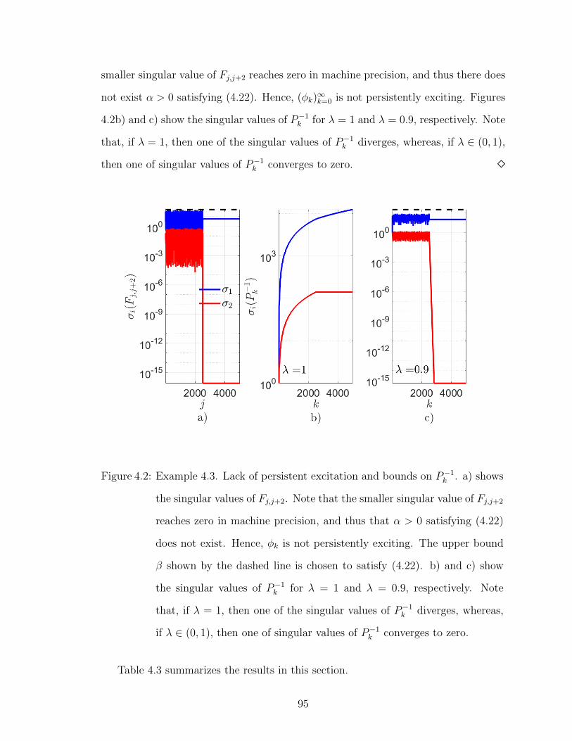
smaller singular value of Fj,j+2 reaches zero in machine precision, and thus there does
not exist α > 0 satisfying (4.22). Hence, (φk)∞k=0 is not persistently exciting. Figures
4.2b) and c) show the singular values of P−1k for λ = 1 and λ = 0.9, respectively. Note
that, if λ = 1, then one of the singular values of P−1k diverges, whereas, if λ ∈ (0, 1),
then one of singular values of P−1k converges to zero. �
Figure 4.2: Example 4.3. Lack of persistent excitation and bounds on P−1k . a) shows
the singular values of Fj,j+2. Note that the smaller singular value of Fj,j+2
reaches zero in machine precision, and thus that α > 0 satisfying (4.22)
does not exist. Hence, φk is not persistently exciting. The upper bound
β shown by the dashed line is chosen to satisfy (4.22). b) and c) show
the singular values of P−1k for λ = 1 and λ = 0.9, respectively. Note
that, if λ = 1, then one of the singular values of P−1k diverges, whereas,
if λ ∈ (0, 1), then one of singular values of P−1k converges to zero.
Table 4.3 summarizes the results in this section.
95

Excitation \ λ λ = 1 λ ∈ (0, 1)Persistent
• Pk converges to zero • Pk remains bounded
• Proposition 4.3 • Propositions 4.4, 4.5
• Example 4.2 • Example 4.2Not Persistent
• Some singular values of Pkremain bounded
• Some singular values of Pkdiverge
• Other singular values of Pkconverge to zero
• Other singular values of Pkremain bounded
• Example 4.3 • Example 4.3
Table 4.3: Behavior of Pk under persistent and not persistent excitation.
4.3 Persistent Excitation and the Condition Number
For nonsingular A ∈ Rn×n, the condition number of A is defined by
κ(A)4=σmax(A)
σmin(A), (4.31)
For B ∈ Rn×m, let ‖B‖ denotes the maximum singular value of B. If A is positive
definite, then
‖A−1‖−1In = σmin(A)In ≤ A ≤ σmax(A)In = ‖A‖In. (4.32)
Therefore, if α, β ∈ (0,∞) satisfy α ≤ σmin(A) and σmax(A) ≤ β, then κ(A) ≤ β
α.
Thus, if λ = 1 and (φk)∞k=0 is persistently exciting with N,α, β given by Definition
4.1, then it follows from (4.24) that
κ(Pk) ≤β
α. (4.33)
96

Similarly, if λ ∈ (0, 1) and (φk)∞k=0 is persistently exciting with N,α, β given by
Definition 4.1, then it follows from (4.28) that
κ(Pk) ≤β + (1− λN+1)‖P−1N ‖
λN(1− λ)α. (4.34)
However, as shown by Example 4.3, if (φk)∞k=0 is not persistently exciting, then there
may not exist α > 0 satisfying (4.22), and thus κ(Pk) cannot be bounded. Hence κ(Pk)
can be used to determine whether or not the (φk)∞k=0 is persistently exciting, where
a bounded condition number implies that (φk)∞k=0 is persistently exciting, whereas a
diverging condition number implies that φk is not persistently exciting, as illustrated
by the following example. [88] provides a recursive algorithm for computing κ(Pk).
Example 4.4. Using the condition number of Pk to determine whether
(φk)∞k=0 is persistently exciting. Consider the 5th-order IIR system
yk =0.68q4 − 0.16q3 − 0.12q2 − 0.18q + 0.09
q5 − q4 + 0.41q3 − 0.17q2 − 0.03q + 0.01uk, (4.35)
where q is the forward-shift operator, and uk is given by (4.30). To apply RLS, let θ
consist of the coefficients in (4.35) and
φk = [uk−1 · · · uk−5 yk−1 · · · yk−5], (4.36)
Note that the regressor (4.36) corresponds to a 5th-order IIR parameterization of a
linear input-output model. Let P0 = I10. Figure 4.3a) shows the singular values of
Fj,j+20, where the singular values of Fj,j+20 close to machine precision (∼ 10−15) are
essentially zero. Thus, Definition 4.1 implies that (φk)∞k=0 is not persistently exciting.
Figures 4.3b) and c) show the singular values and the condition number of Pk for
λ = 1. Note that the six singular values of Pk decrease due to the presence of three
harmonics in uk. Note that κ(Pk) is diverging due to the lack of persistent excitation.
97

Figures 4.3d) and e) show the singular values and the condition number of Pk
for λ = 0.99. Note that the six singular values of Pk remain bounded due to the
presence of three harmonics in uk. However, Pk becomes ill-conditioned due to the
lack of persistent excitation. Consequently, numerical computation with Pk becomes
erroneous once Pk becomes ill-conditioned. �
98

Figure 4.3: Example 4.4. Using the condition number of Pk to evaluate persistency.
a) shows the singular values of Fj,j+20, where the singular values of Fj,j+20
close to machine precision (∼ 10−15) are essentially zero, thus implying
that (φk)∞k=0 is not persistently exciting. b) and c) shows the singular
values and the condition number of Pk for λ = 1. Note that the six
singular values of Pk decrease due to the presence of three harmonics in
uk. d) and e) shows the singular values and the condition number of Pk
for λ = 0.99. Note that the six singular values of Pk remain bounded
due to the presence of three harmonics in uk. However, Pk becomes ill-
conditioned due to the lack of persistent excitation.
99
Example 4.4 shows that if (φk)∞k=0 is not persistently exciting and λ = 1, then some
singular values of Pk converge while the rest decrease to zero. On the other hand,
if (φk)∞k=0 is not persistent and λ ∈ (0, 1), then some singular values of Pk diverge
while the rest remain bounded. In particular, let (φk)∞k=0 be not persistent such that,
for λ = 1, n1 singular values of Pk converge to zero, while n − n1 remain bounded.
Then, for λ ∈ (0, 1), n1 singular values remain bounded, while n− n1 singular values
diverge.
4.4 Lyapunov Analysis of the Parameter Error
Let k ≥ 0, and consider the system
xk+1 = f(k, xk), (4.37)
where xk ∈ Rn, f : {0, 1, 2, . . .}×Rn → Rn is continuous, and, for all k ≥ 0, f(k, 0) =
0.
Definition 4.2. The zero solution xk ≡ 0 of (4.37) is uniformly Lyapunov stable if,
for all ε > 0, there exists δ ∈ (0, ε] such that, for all k0 ≥ 0 and all xk0 ∈ Rn such
that ‖xk0‖ < δ, it follows that, for all k ≥ k0, ‖xk‖ < ε.
Definition 4.3. The zero solution xk ≡ 0 of (4.37) is uniformly globally aymptot-
ically stable if it is uniformly Lyapunov stable, and for all x0 ∈ Rn, if follows that
limk→∞ xk = 0.
Definition 4.4. The zero solution xk ≡ 0 of (4.37) is uniformly globally geometrically
stable if there exist α0 > 0 and β0 > 1 such that, for all x0 ∈ Rn, it follows that, for
all k ≥ 0,
‖xk‖ ≤ α0‖x0‖β−k0 . (4.38)
100

Note that, if the zero solution xk ≡ 0 of (4.37) is uniformly globally geometri-
cally stable, then it is uniformly globally aymptotically stable as well as uniformly
Lyapunov stable.
The following result is a specialization of Theorem 13.11 given in [89, pp. 784,
785].
Theorem 4.2. Consider (4.37), and assume there exist a continuous function V :
Rn → R and α1, β1 > 0 such that, for all k ≥ 0,
α1‖x‖2 ≤ V (k, x) ≤ β1‖x‖2, (4.39)
V (k + 1, f(k, x))− V (k, x) ≤ 0. (4.40)
Then the zero solution xk ≡ 0 of (4.37) is uniformly Lyapunov stable. Furthermore,
assume there exists γ1 > 0 such that, for all k ≥ 0 and x ∈ Rn,
V (k + 1, f(k, x))− V (k, x) ≤ −γ1‖x‖2. (4.41)
Then the zero solution xk ≡ 0 of (4.37) is uniformly globally geometrically stable.
The following result uses Lyapunov theory to show that, if (φk)∞k=0 is persistently
exciting, then the RLS estimate θk with λ ∈ (0, 1) converges to θ in the sense of
Definition 4.4. A related result is given in [87].
Theorem 4.3. Assume that (φk)∞k=0 is persistently exciting, let N,α, β be given by
Definition 4.1, let R ∈ Rn×n be positive definite, define P04= R−1, let λ ∈ (0, 1], and,
for all k ≥ 0, let Pk be given by (4.4). Then the zero solution of (4.10) is Lyapunov
stable. In addition, if λ ∈ (0, 1), then the zero solution of (4.10) is uniformly globally
geometrically stable.
101
Proof. Define the Lyapunov candidate
V (k, x)4= xTP−1k x,
where x ∈ Rn. It follows from Proposition 4.4 that, for all k ≥ N + 1,
λN(1− λ)α
1− λN+1‖x‖2 ≤ V (k, x) ≤ β
1− λN+1‖x‖2 + xTP−1N x
≤(
β
1− λN+1+ ‖P−1N ‖
)‖x‖2,
which confirms (4.39) for all λ ∈ (0, 1] with α1 = λN (1−λ)α1−λN+1 , and β1 = β
1−λN+1 + ‖P−1N ‖.
Next, defining
f(k, x)4= (In − Pk+1φ
Tk φk)x,
it follows that
V (k + 1, f(k, x))− V (k, x) = f(k, x)TP−1k+1f(k, x)− xTP−1k x
= xT[(In − φTk φkPk+1)P
−1k+1(In − Pk+1φ
Tk φk)− P−1k ]x
= xT[(P−1k+1 − φTk φk)(In − Pk+1φ
Tk φk)− P−1k ]x
= xT[(λ− 1)P−1k − λP−1k Pk+1φ
Tk φk]x
= xT[(λ− 1)P−1k − λφTk (λIp − φkPkφT
k )−1φk]x.
≤ 0,
which confirms (4.40). It thus follows from Theorem 4.2 that the zero solution of
(4.10) is uniformly Lyapunov stable.
102
Furthermore, if λ ∈ (0, 1), then
V (k + 1, f(k, x))− V (k, x) ≤ (λ− 1)xTP−1k x
≤ (λ− 1)
(β
1− λN+1+ ‖P−1N ‖
)‖x‖2,
which confirms (4.41) with γ1 = (1−λ)( β1−λN+1 +‖P−1N ‖). It thus follows from Theorem
4.2 that the zero solution of (4.10) is uniformly globally geometrically stable.
The following result provides an alternative proof of Theorem 4.3 that does not
depend on Theorem 4.2. In addition, this result considers the case λ = 1, where the
RLS estimate θk converges to θ in the sense of Definition 4.3.
Theorem 4.4. Assume that (φk)∞k=0 is persistently exciting, let N,α, β be given by
Definition 4.1, let R ∈ Rn×n be positive definite, define P04= R−1, let λ ∈ (0, 1], and,
for all k ≥ 0, let Pk be given by (4.4). Then the zero solution of (4.10) is uniformly
globally asymptotically stable. Furthermore, if λ ∈ (0, 1), then the zero solution of
(4.10) is uniformly globally geometrically stable.
Proof. Let k0 ≥ 0 and θk0 ∈ Rn. Then, it follows from (4.12) that, for all k ≥ k0,
‖θk‖ = λk−k0‖PkP−1k0θk0‖
≤ ‖PkP−1k0θk0‖
≤ ‖Pk‖‖P−1k0‖‖θk0‖. (4.42)
First, consider the case where λ = 1. Let δ > 0, and suppose that θk0 ∈ Rn satisfies
‖θk0‖ ≤ δ. Now note that it follows from (4.6) with λ = 1 that Pk ≤ Pk−1 ≤ · · · ≤ Pk0 .
Hence, for all k ≥ k0, ‖Pk‖ ≤ ‖Pk0‖, and thus ‖Pk‖‖P−1k0‖ = ‖Pk‖/‖Pk0‖ ≤ 1. It
thus follows from (4.42) that, for all k ≥ k0, ‖θk‖ ≤ ‖θk0‖ < δ.It thus follows from
Definition 4.2 with ε = δ that the zero solution of (4.10) is uniformly Lyapunov
stable.
103

Next, let θ0 ∈ Rn. Then, Proposition 4.3 implies that
limk→∞
θk = limk→∞
PkP−10 θ0 = 0.
It thus follows from Definition 4.3 that the zero solution of (4.10) is uniformly globally
asymptotically stable.
Next, consider the case where λ ∈ (0, 1). Let k0 ≥ 0 and δ > 0, and let θk0 ∈ Rn
satisfy ‖θk0‖ ≤ δ. It follows from Proposition 4.4 and (4.42) that, for all k ≥ max(N+
1, k0),
‖θk‖ ≤ ε,
where
ε4=β + (1− λN+1)‖P−1N ‖
λN(1− λ)αδ.
It thus follows from Definition 4.2 that the zero solution of (4.10) is uniformly Lya-
punov stable.
Next, let θ0 ∈ Rn. Then, it follows from (4.12) and Proposition 4.4 that, for all
θ0 ∈ Rn, and k ≥ N + 1,
‖θk‖ ≤ α0‖θ0‖β−k0 ,
where β04= 1/λ and
α04=
1− λN+1
λN(1− λ)α‖P−10 ‖.
Thus, it follows from Definition 4.4 that the zero solution of (4.10) is uniformly
globally geometrically stable, and thus uniformly globally asymptotically stable.
104

The following result shows that persistent excitation produces an infinite sequence
of matrices whose product converges to zero.
Proposition 4.6. Let P0 ∈ Rn×n be positive definite, let λ ∈ (0, 1], and, for all k ≥ 0,
let Pk be given by (4.4). Then, for all k ≥ 0, all of the eigenvalues of Pk+1φTk φk are
contained in [0, 1]. If, in addition, (φk)∞k=0 is persistently exciting, then
limk→∞
Ak = 0, (4.43)
where
Ak4= (In − Pk+1φ
Tk φk) · · · (In − P1φ
T0 φ0). (4.44)
Proof. It follows from (4.6) that, for all k ≥ 0, φTk φk ≤ P−1k+1, and thus, for all k ≥ 0,
P1/2k+1φ
Tk φkP
1/2k+1 ≤ In. Hence, for all k ≥ 0,
0 ≤ λmax(Pk+1φTk φk) = λmax(P
1/2k+1φ
Tk φkP
1/2k+1) ≤ 1.
To prove (4.43), suppose that (φk)∞k=0 is persistently exciting and, for all i ∈ {1, . . . , n},
define θ04= ei + θ, where ei is the ith column of In. Note that, for all i ∈ {1, . . . , n},
θ04= θ0 − θ = ei. Then, (4.12) implies that, for all k ≥ 0 and all i ∈ {1, . . . , n},
θk+1 = Akei = λk+1Pk+1P−10 ei.
It follows from Proposition 4.4 that, for all i ∈ {1, . . . , n}, θk converges to 0. Hence,
for all i ∈ {1, . . . , n}, the ith column of Ak converges to zero as k →∞, which implies
(4.43).
It follows from Proposition 4.4 that, if (φk)∞k=0 is persistently exciting, then, for
all λ ∈ (0, 1], θk converges to zero. In addition, if λ ∈ (0, 1), then θk converges to zero
105

geometrically, that is, the rate of convergence of ‖θk‖ is O(λk). However, in the case
λ = 1, as shown in [87] and the next example, θk converges to zero as O(1/k), and
thus the convergence is not geometric.
Example 4.5. Effect of λ on the rate of convergence of θk. Consider the
3rd-order FIR system
yk =q2 + 0.8q + 0.5
q3uk, (4.45)
where q is the forward-shift operator. To apply RLS, let θ = [1 0.8 0.5], θ0 = 0, and
φk = [uk−1 uk−2 uk−3], where the input uk is zero-mean Gaussian white noise with
unity standard deviation. Figures 4.4a) - f) show the parameter error norm ‖θk‖ for
several values of P0 and λ. Note that the convergence rate of ‖θk‖ is O(1/k) for λ = 1
and geometric for all λ ∈ (0, 1). Figures 4.4g), h), and i) show the condition number
of the corresponding Pk for several values of P0 and λ. Note that, as λ is decreased,
the convergence rate of θk increases; however, the condition number of Pk degrades,
and the effect of P0 is reduced. �
106
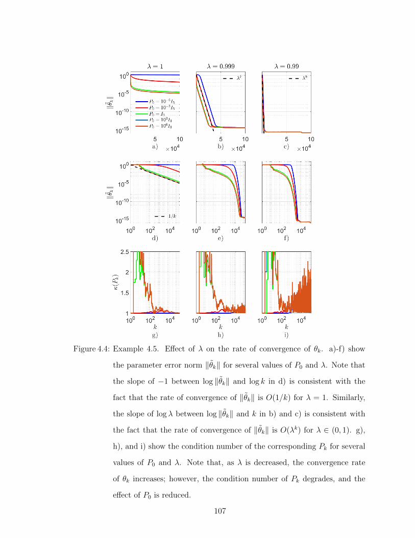
Figure 4.4: Example 4.5. Effect of λ on the rate of convergence of θk. a)-f) show
the parameter error norm ‖θk‖ for several values of P0 and λ. Note that
the slope of −1 between log ‖θk‖ and log k in d) is consistent with the
fact that the rate of convergence of ‖θk‖ is O(1/k) for λ = 1. Similarly,
the slope of log λ between log ‖θk‖ and k in b) and c) is consistent with
the fact that the rate of convergence of ‖θk‖ is O(λk) for λ ∈ (0, 1). g),
h), and i) show the condition number of the corresponding Pk for several
values of P0 and λ. Note that, as λ is decreased, the convergence rate
of θk increases; however, the condition number of Pk degrades, and the
effect of P0 is reduced.
107
4.5 Lack of Persistent Excitation
In this section, we investigate the effect of lack of persistent excitation on Pk and
θk using numerical examples. Recall that, as shown in Example 4.3 and Example
4.4, if (φk)∞k=0 is not persistently exciting and λ = 1, then some singular values of
Pk converge to zero, while the rest remain bounded. On the other hand, if (φk)∞k=0
is not persistently exciting and λ ∈ (0, 1), then some singular values of Pk remain
bounded, while the rest diverge. Furthermore, it follows from Proposition 4.1 that
the predicted error zk and the parameter error θk converge to zero, irrespective of
whether (φk)∞k=0 is persistent or not.
Example 4.6. Lack of persistent excitation in scalar estimation. Let n = 1,
so that (4.4), (4.5) are given by
Pk+1 =Pk
λ+ Pkφ2k
, (4.46)
θk+1 =λθk
λ+ Pkφ2k
. (4.47)
Now, let k0 ≥ 0 and assume that, for all k ≥ k0, φk = 0. Therefore, for all j ≥
0 and N ≥ 1, Fj,j+N cannot be lower bounded as in (4.22), and thus (φk)∞k=0 is
not persistently exciting. For λ = 1, Pk and θk converge in k0 steps to P and θ,
respectively, where P 6= 0 and, if θ0 6= θ, then θ 6= 0. However, for all λ ∈ (0, 1), Pk
diverges geometrically and θk converges in k0 steps.
Note that, for all λ ∈ (0, 1], since φk = 0 for all k ≥ k0, it follows from (4.46) and
(4.47) that, for all k ≥ k0, the minimum of (4.2) is achieved in a finite number of
steps. Consequently, RLS provides no further refinement of the estimate θk of θ, and
thus θ 6= 0 implies that θk does not converge to θ.
Next, assume that, for all k ≥ 0, φk = φ, where φ 6= 0. Then Definition 4.1
is satisfied with N = 1, α = φ2, and β = 3φ
2, and thus (φk)
∞k=0 is persistently
108

exciting. If λ = 1, then both Pk and θk converge to zero. However, if λ ∈ (0, 1),
then Pk converges to 1−λφ2 and θk converges geometrically to zero. Table 4.4 shows the
asymptotic behavior of θk and Pk for various cases. �
Excitation \ λ λ = 1 λ ∈ (0, 1)
Not persistently exciting θk → θ, Pk → P θk → θ, Pk diverges
Persistently exciting θk → 0, Pk → 0 θk → 0, Pk → 1−λφ2
Table 4.4: Asymptotic behavior of RLS in Example 4.6. In the case of persistentexcitation with λ < 1, the convergence of θk is geometric.
Example 4.7. Subspace constrained regressor. Consider (4.1), where φk =
(sin 2πk100
)[1 1] and θ = [0.4 1.4]T. To estimate θ using RLS, let P0 = I2 and θ0 = 0.
Figures 4.5 and 4.6 show the estimate θk of θ with λ = 1 and λ = 0.99. Note that
all regressors φk lie along the same one-dimensional subspace, and thus, (φk)∞k=0 is
not persistently exciting. It follows from (4.19) that the estimate θk of θ lies in this
subspace.
For λ = 1, note that one of the singular value decreases to zero, while the other
singular value remains bounded. Note that θk converges along the singular vector
corresponding to the bounded singular value. For λ = 0.99, one of the singular value
remains bounded, while the other singular value diverges. Note that θk converges
along the singular vector corresponding to the diverging singular value. �
109
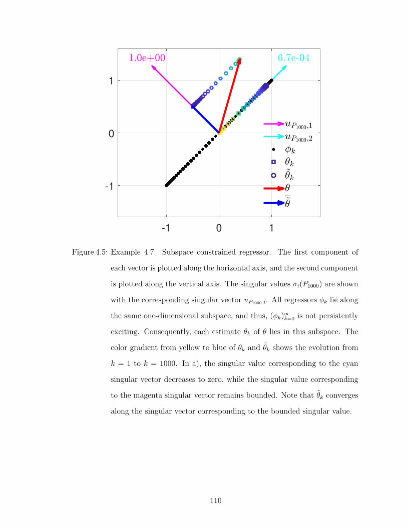
-1 0 1
-1
0
1
Figure 4.5: Example 4.7. Subspace constrained regressor. The first component of
each vector is plotted along the horizontal axis, and the second component
is plotted along the vertical axis. The singular values σi(P1000) are shown
with the corresponding singular vector uP1000,i. All regressors φk lie along
the same one-dimensional subspace, and thus, (φk)∞k=0 is not persistently
exciting. Consequently, each estimate θk of θ lies in this subspace. The
color gradient from yellow to blue of θk and θk shows the evolution from
k = 1 to k = 1000. In a), the singular value corresponding to the cyan
singular vector decreases to zero, while the singular value corresponding
to the magenta singular vector remains bounded. Note that θk converges
along the singular vector corresponding to the bounded singular value.
110

-1 0 1
-1
0
1
Figure 4.6: Example 4.7. Subspace constrained regressor. The first component of
each vector is plotted along the horizontal axis, and the second compo-
nent is plotted along the vertical axis. The singular values σi(P1000) are
shown with the corresponding singular vector uP1000,i. All regressors φk lie
along the same one-dimensional subspace, and thus, (φk)∞k=0 is not persis-
tently exciting. Consequently, each estimate θk of θ lies in this subspace.
The color gradient from yellow to blue of θk and θk shows the evolution
from k = 1 to k = 1000. The singular value corresponding to the cyan
singular vector remains bounded, while the singular value corresponding
to the magenta singular vector diverges. Note that θk converges along the
singular vector corresponding to the diverging singular value.
Example 4.8. Lack of persistent excitation and finite-precision arithmetic.
Consider the problem of fitting a 5th-order IIR model to the measured input-output
data from the system (4.35), where the input uk is given by (4.30). Note that φk
111

is given by (4.36), and is not persistently exciting as shown in Example 4.4. Let
P0 = I10, θ0 = 0, and λ = 0.999. Figure 4.7a) shows the predicted error zk, and b)
shows the norm of the parameter error θk. Note that the θk does not converge to 0.
c) shows the singular values of Pk, and d) shows the condition number of Pk. Note
that six singular values of Pk remain bounded due to the presence of three harmonics
in the regresssor. Due to finite-precision arithmetic, computation becomes erroneous
as Pk becomes numerically ill-conditioned, and thus, the estimate θk diverges. �
112

Figure 4.7: Example 4.8. Effect of lack of persistent excitation on θk. a) shows
the predicted error zk, b) shows the norm of the parameter error θk,
c) shows the singular values of Pk, and d) shows the condition number
of Pk. Note that six singular values of Pk remain bounded due to the
presence of three harmonics in the regresssor. Due to finite-precision
arithmetic, computation becomes erroneous as Pk becomes numerically
ill-conditioned, and thus, the estimate θk diverges.
The numerical examples in this section show that, if λ ∈ (0, 1] and (φk)∞k=0 is not
persistently exciting, then θk does not necessarily converge to zero. Furthermore, if
λ ∈ (0, 1) and (φk)∞k=0 is not persistently exciting, then some singular values of Pk di-
113
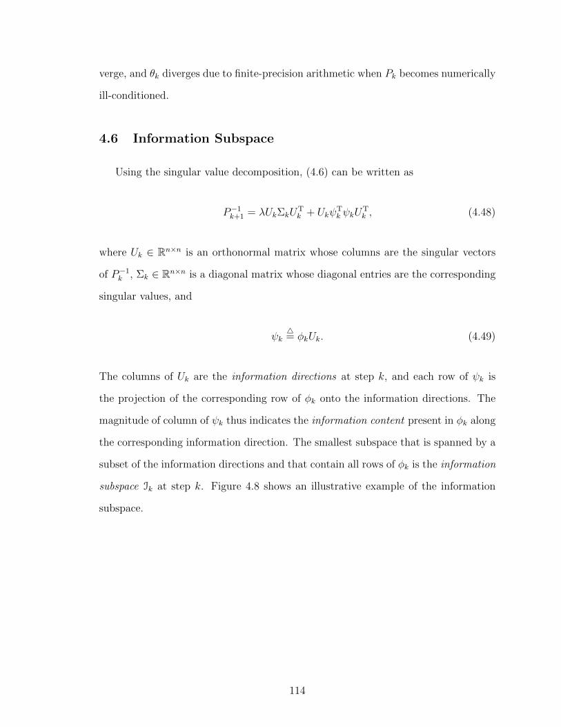
verge, and θk diverges due to finite-precision arithmetic when Pk becomes numerically
ill-conditioned.
4.6 Information Subspace
Using the singular value decomposition, (4.6) can be written as
P−1k+1 = λUkΣkUTk + Ukψ
Tk ψkU
Tk , (4.48)
where Uk ∈ Rn×n is an orthonormal matrix whose columns are the singular vectors
of P−1k , Σk ∈ Rn×n is a diagonal matrix whose diagonal entries are the corresponding
singular values, and
ψk4= φkUk. (4.49)
The columns of Uk are the information directions at step k, and each row of ψk is
the projection of the corresponding row of φk onto the information directions. The
magnitude of column of ψk thus indicates the information content present in φk along
the corresponding information direction. The smallest subspace that is spanned by a
subset of the information directions and that contain all rows of φk is the information
subspace Ik at step k. Figure 4.8 shows an illustrative example of the information
subspace.
114
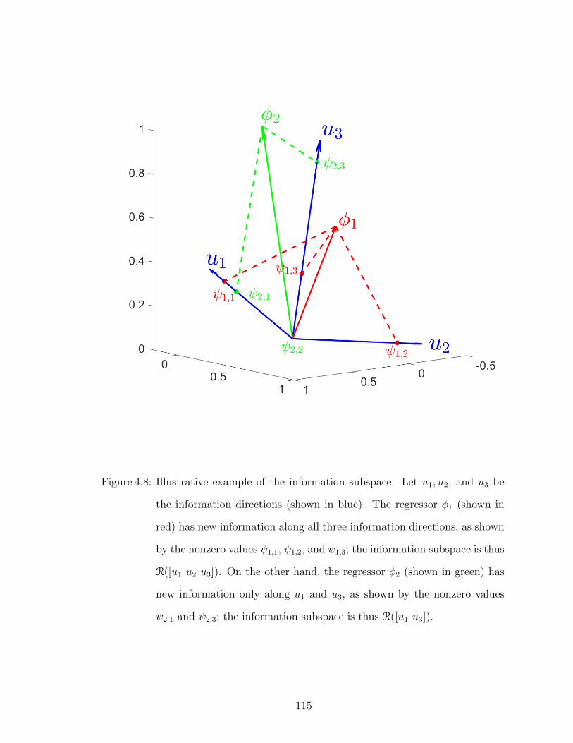
Figure 4.8: Illustrative example of the information subspace. Let u1, u2, and u3 be
the information directions (shown in blue). The regressor φ1 (shown in
red) has new information along all three information directions, as shown
by the nonzero values ψ1,1, ψ1,2, and ψ1,3; the information subspace is thus
R([u1 u2 u3]). On the other hand, the regressor φ2 (shown in green) has
new information only along u1 and u3, as shown by the nonzero values
ψ2,1 and ψ2,3; the information subspace is thus R([u1 u3]).
115

Now, consider the case where
ψk =
[ψk,1 0p×(n−n1)
], (4.50)
where ψk,1 ∈ Rp×n1 , which implies that φk provides new information along the first n1
columns of Uk; these directions constitute the information subspace. It thus follows
from (4.48) and (4.50) that P−1k+1 is given by
P−1k+1 = Uk
λΣk,1 + ψTk,1ψk,1 0
0 λΣk,2
UTk , (4.51)
where Σk,1 ∈ Rn1×n1 is the diagonal matrix whose diagonal entries are the first n1
singular values of P−1k , and Σk,2 is the diagonal matrix whose diagonal entries are the
remaining n− n1 singular values of P−1k . In particular, writing
Uk =
[Uk,1 Uk,2
], (4.52)
where Uk,1 ∈ Rn×n1 contains the first n1 columns of Uk, and Uk,2 ∈ Rn×n−n1 contains
the remaining n− n1 columns of Uk, it follows that
P−1k+1 =
[Uk+1,1 Uk+1,2
] Σk+1,1 0
0 Σk+1,2
UT
k+1,1
UTk+1,2
, (4.53)
where
Uk+1,1 = Uk,1Vk, (4.54)
Σk+1,1 = Dk, (4.55)
Uk+1,2 = Uk,2, (4.56)
Σk+1,2 = λΣk,2, (4.57)
116

where Vk ∈ Rn1×n1 contains the singular vectors of λΣk,1 + ψTk,1ψk,1 and Dk ∈ Rn1×n1
is the diagonal matrix containing the corresponding singular values. It follows from
(4.56), (4.57) that if, for all k ≥ 0, ψk is given by (4.50) and λ ∈ (0, 1), then the last
n−n1 singular vectors of P−1k do not change and the corresponding singular values of
P−1k decrease to zero geometrically. It thus follows from Proposition 4.4 that (φk)∞k=0
is not persistently exciting. Furthermore, since Pk and P−1k have the same singular
vectors and the singular values of Pk are the inverse of the singular values of P−1k , the
last n− n1 singular values of Pk diverge.
The following example shows that, if (φk)∞k=0 is not persistently exciting, then
the information subspace is a proper subset of Rn and the singular values of P−1k
corresponding to the singular vectors in the orthogonal complement of the information
subspace converge to zero.
Example 4.9. Lack of persistent excitation and the information subspace .
Consider the regressor φk given by (4.36) used in Example 4.4. Recall that (φk)∞k=0 is
not persistently exciting. Let P0 = I10. Figures 4.9a), b), and c) show the informa-
tion content |ψk,i| for several values of λ. Note that the information subspace is six
dimensional due to the presence of three harmonics in uk as shown by six relatively
large components of ψk. Figures 4.9d), e), and f) show the singular values of P−1k
for several values of λ. Note that, for λ < 1, the singular values that correspond
to the singular vectors not in the information subspace convergeto zero in machine
precision. �
4.7 Information-Driven Forgetting
Motivated by the fact that some singular values of P−1k converge to zero if φk is
not persistently exciting, as shown in Examples 4.3, 4.4, 4.6, 4.7, and 4.8, we propose
the following modification. We modify (4.6) by replacing the scalar forgetting factor
117

λ by a data-dependent forgetting matrix Λk. To do this, we redefine P−1k+1 as
P−1k+1 = ΛkP−1k Λk + φT
k φk, (4.58)
where Λk is a positive-definite (and thus symmetric) matrix constructed below. Note
that, for all k ≥ 0, P−1k+1 given by (4.58) is positive-definite. Using the singular value
decomposition, (4.58) can be written as
P−1k+1 = ΛkUkΣkUTk Λk + Ukψ
Tk ψkU
Tk , (4.59)
where Uk, Σk, and ψk are as defined in the previous section.
The objective is to apply forgetting to only those singular values of P−1k that
correspond to the singular vectors in the information subspace, that is, forgetting
is restricted to the subspace of P−1k where sufficient new information is provided
by φk. Specifically, forgetting is applied to those information directions where the
information content is greater than ε > 0, where ε should be selected to be larger
than the noise to signal ratio or larger than the machine zero, if no noise is present.
To do so, we write (4.59) as
P−1k+1 = UkΛkΣkΛkUTk + Ukψ
Tk ψkU
Tk , (4.60)
where Λk is a diagonal matrix whose diagonal entries are either√λ or 1. In particular,
Λk(i, i)4=
√λ, ‖ψk,i‖ > ε,
1, otherwise,
(4.61)
where ψk,i is the ith column of ψk and λ ∈ (0, 1]. Next, it follows from (4.59), (4.60)
118

that
Λk = UkΛkUTk , (4.62)
which is positive definite.
Using Uk obtained by the singular value decomposition of Pk, the information
content ψk given by (4.49), Λk is given by (4.61), and applying the matrix inversion
lemma to (4.58), the recursive update of Pk is given by
Λ−1k = UkΛ−1k UT
k , (4.63)
P k = Λ−1k PkΛ−1k , , (4.64)
Pk+1 = P k − P kφk(Ip + φTkP kφk)
−1φTkP k. (4.65)
Next, we show that the forgetting scheme (4.63) in (4.65) prevents the singular
values of Pk from diverging. Consider the case where, for all k,
ψk =
[ψk,1 0
], (4.66)
where ψk,1 ∈ Rp×n1 , that is, the information subspace is spanned by the first columns
of Uk. It thus follows from (4.60) and (4.66) that P−1k+1 is given by
P−1k+1 = Uk
λΣk,1 + ψTk,1ψk,1 0
0 Σk,2
UTk . (4.67)
It follows from the (2, 2) block of (4.67) that the last n−n1 information directions and
the corresponding singular values are not affected by φk. Furthermore, if n1 = n, that
is, new information is present in φk along every information direction, then forgetting
is applied to all of the singular values of P−1k , and thus information-driven directional
forgetting specializes to spatially uniform forgetting, that is, RLS with the update for
119

Pk given by (4.6).
Example 4.10. Information-driven forgetting for a regressor lacking per-
sistent excitation. Reconsider Example 4.9. Let P0 = I10, and P−1k be given by
(4.65), where ε = 10−8. Figures 4.10a) and b) show the information content |ψk,i| for
several values of λ. Note that the information subspace is six dimensional due to the
presence of three harmonics in uk as shown by six relatively large components of ψk.
Figures 4.10c) and d) show the singular values of P−1k for several values of λ. Note
that the singular values that correspond to the singular vectors not in the information
subspace do not convergeto zero. �
120
Figure 4.10: Example 4.10. Information-driven forgetting for a regressor lacking per-
sistent excitation. a) and b) show the information content ‖ψk‖ for
λ = 0.9 and λ = 0.8. c) and d) show the singular values of P−1k for
λ = 0.9 and λ = 0.8. The inverse of the condition number of Pk is
shown in black. Note that, for λ < 1, the singular values that corre-
spond to the singular vectors not in the information subspace do not
converge to zero.
Example 4.11. Effect of information-driven forgetting on θk. Reconsider
Example 4.8. Let P0 = I10, and P−1k be given by (4.65), where ε = 10−8. Figure
4.11a) shows the predicted error zk, and b) shows the norm of the parameter error
121

θk. Note that the θk does not converge to 0. c) shows the singular values of Pk, and
d) shows the condition number of Pk. Note that, unlike spatially uniform forgetting,
all singular values of Pk remain bounded, and θk does not diverge. �
Figure 4.11: Example 4.11. Effect of Information-driven forgetting on θk. a) shows
the predicted error zk, b) shows the norm of the parameter error θk, c)
shows the singular values of Pk, and d) shows the condition number of
Pk. Note that all singular values of Pk remain bounded.
122

Figure 4.9: Example 4.9. Relation between Pk and the information content ψk. a),b), and c) show the information content ψk,i for several values of λ. Notethat, in each case, the information subspace is six dimensional due to thepresence of three harmonics in uk. d), e), and (f) show the singular valuesof P−1k for several values of λ. The inverse of the condition number ofPk is shown in black. Note that, for λ < 1, the singular values of P−1k
corresponding to the singular vectors in the orthogonal complement ofthe information subspace converge to zero.
123
4.8 Conclusions
This chapter presented various results on uniform and directional forgetting within
the context of RLS. It was shown that, in the case of persistent excitation without
forgetting, the parameter estimates converge asymptotically, whereas, with forgetting,
the parameter estimates converge geometrically. Numerical examples were presented
to illustrate this behavior.
In the case where the excitation is not persistent and forgetting is used, it was
shown that forgetting is enforced in all information directions, whether or not new in-
formation is present in along all information directions. Consequently, the parameter
estimates converge, but not necessarily to their true values; furthermore, the matrix
Pk diverges leading to numerical instability. This phenomenon was traced to the di-
vergence of the singular values of Pk corresponding to singular vectors orthogonal to
the information subspace.
In order to address this problem, a data-dependent forgetting matrix was con-
structed to restrict forgetting to the information subspace. Numerical examples pre-
sented show that this directional forgetting technique prevents Pk from diverging
under lack of persistent excitation.
124

CHAPTER 5
Adaptive Squaring-Based Control Allocation for
Wide Systems
5.1 Introduction
Redundant actuators provide the opportunity to allocate control effort to account
for saturation and other input constraints. This is especially true in wide systems,
where the number of input channels is greater than the number of outputs. The
present chapter considers the control allocation problem within the context of adap-
tive control.
Many control applications possess the mixed blessing of more actuators than con-
trolled outputs. For these applications, the required control inputs can be realized by
combinations of redundant actuators, thus providing reliability. At the same time,
however, the presence of actuators with similar effect on the system demands that
these actuators be used optimally with respect to magnitude and rate saturation,
energy usage, and other limitations. This is the control allocation problem [90, 91].
Control allocation is widely studied within the context of aerospace vehicles [92–
95], where the moments obtainable from control surfaces are limited by there size and
depend on the current the aircraft speed. A classical case of actuator redundancy in
lateral flight control concerns the use of ailerons and rudders to perform turning
125

maneuvers. Separate use of these actuators for turning yields poor performance, due
to adverse aileron yaw and adverse rudder roll. Consequently, control allocation can
ensure that the ailerons and rudder are used in a desirable combination to perform
coordinated turns.
In the present chapter, we consider control allocation within the context of retro-
spective cost adaptive control (RCAC) [96]. RCAC is a direct digital control technique
that is applicable to stabilization, command following, and disturbance rejection. A
key feature of RCAC discussed in [96] is the role of the filter Gf in defining the
retrospective cost variable. As shown in [96], Gf serves as a target model for the
intercalated transfer function from the virtual external control perturbation to the
performance variable. Modeling information concerning the leading numerator sign,
relative degree, and nonminimum-phase (NMP) zeros is used to construct Gf .
The present chapter extends the development of [96] by focusing on wide (that is,
overactuated) systems for the purpose of control allocation. In particular, we show
that the applied control input lies in the range of the target model. For example, if
the plant is MISO and the target model Gf is chosen to be Gf(q) = N11q, where q
is the forward shift operator and N1 is a row vector, then the control input vector is
constrained to the direction NT1 . For example, if the plant has two inputs and one
output andN1 is chosen to beN1 = [3 6], then, for all time steps k, u1(k)/u2(k) = 1/2.
Consequently, the target model provides a simple and convenient technique for control
allocation in overactuated systems.
The contents of the chapter are as follows. Section 5.2 states the control allocation
problem. Next, Section 5.3 reviews RCAC, and Theorem 5.1 demonstrates how the
target model constrains the allowable directions of the control input. Section 5.4
presents several examples illustrating control allocation for RCAC. The chapter ends
with some conclusions and directions for future research.
126
5.2 Control allocation problem
Consider the MIMO discrete-time plant
x(k + 1) = f(x(k), u(k)) +D1w(k), (5.1)
y(k) = g(x(k)) +D2w(k), (5.2)
z(k) = Ex(k) + E0w(k), (5.3)
where x(k) ∈ Rlx is the state, y(k) ∈ Rly is the measurement, u(k) ∈ Rlu is the control
signal, w(k) ∈ Rlw is the exogenous signal, and z(k) ∈ Rlz is the performance variable.
The components of w can represent either command signals to be followed, external
disturbances to be rejected, or both. Figure 5.1 shows a block diagram representation
of (5.1)–5.3.
The goal is to develop an adaptive output-feedback controller that produces the
control effort in a desired ratio and minimizes z in the presence of the exogenous
signal w with limited modeling information about (5.1)–(5.3) .
In this chapter, we consider overactuated systems, that is, lu > ly. In overactuated
systems, the control input required to generate a desired output is not unique. For
example, consider step command following for a two-input, one-output LTI plant. At
steady state,
y∞ = C(I − A)−1Bu∞, (5.4)
where y∞ ∈ R is the asymptotic output of the plant, and u∞ ∈ R2 is the asymptotic
control input. Since C(I − A)−1B is a wide matrix, it follows that the asymptotic
control input u∞ is not unique. The goal of the control allocation problem is thus to
achieve the specified performance objectives while confining the control input vector
u to a chosen subspace that constrains the direction of the allowable control inputs.
127

Gc Gr z u
d
y
v
Figure 5.1: Block diagram representation of the adaptive control allocation problem
with the adaptive controller Gc and plant G. The goal is to design the
controller Gc that produces the control effort in a desired ratio such that
the plant output y follows the reference command r in presence of process
noise d and measurement noise v.
5.3 RCAC algorithm
We consider a dynamic compensator represented by an ARMA model.The control
u(k) is thus given by
u(k) =nc∑i=1
Pi(k)u(k − i) +nc∑i=1
Qi(k)z(k − i), (5.5)
where the coefficient matrices Pi(k) ∈ Rlu×lu , Qi(k), R(k) ∈ Rlu×lz are updated by
the RCAC algorithm.
We rewrite (5.5) as
u(k) = Φ(k)θ(k), (5.6)
128

where the regressor matrix Φ(k) is defined by
Φ(k)4= Ilu ⊗ φT(k) ∈ Rlu×lθ , (5.7)
where
φ(k)4= [µ(k − 1)T · · · µ(k − nc)
T z(k − 1)T · · · z(k − nc)T]T,
θ(k)4= vec
[P1(k) · · ·Pnc(k) Q1(k) · · ·Qnc(k)
]∈ Rlθ ,
lθ4= l2unc + lulync, “⊗” is the Kronecker product, and “vec” is the column-stacking
operator.
5.3.1 Retrospective Performance Variable
We define the retrospective performance variable
z(k) = z(k) +Gf(q)(Φ(k)θ − u(k)), (5.8)
where q is the forward-shift operator, θ ∈ Rlθ contains the controller coefficients to
be optimized,
Gf(q) =
nf∑i=1
Niq−i, (5.9)
and, for all i = 1, . . . , nf , Ni ∈ Rly×lu . Gf is an FIR filter of order nf whose choice is
discussed below. We rewrite (5.8) as
z(k) = z(k) +NΦb(k)θ −NUb(k), (5.10)
129
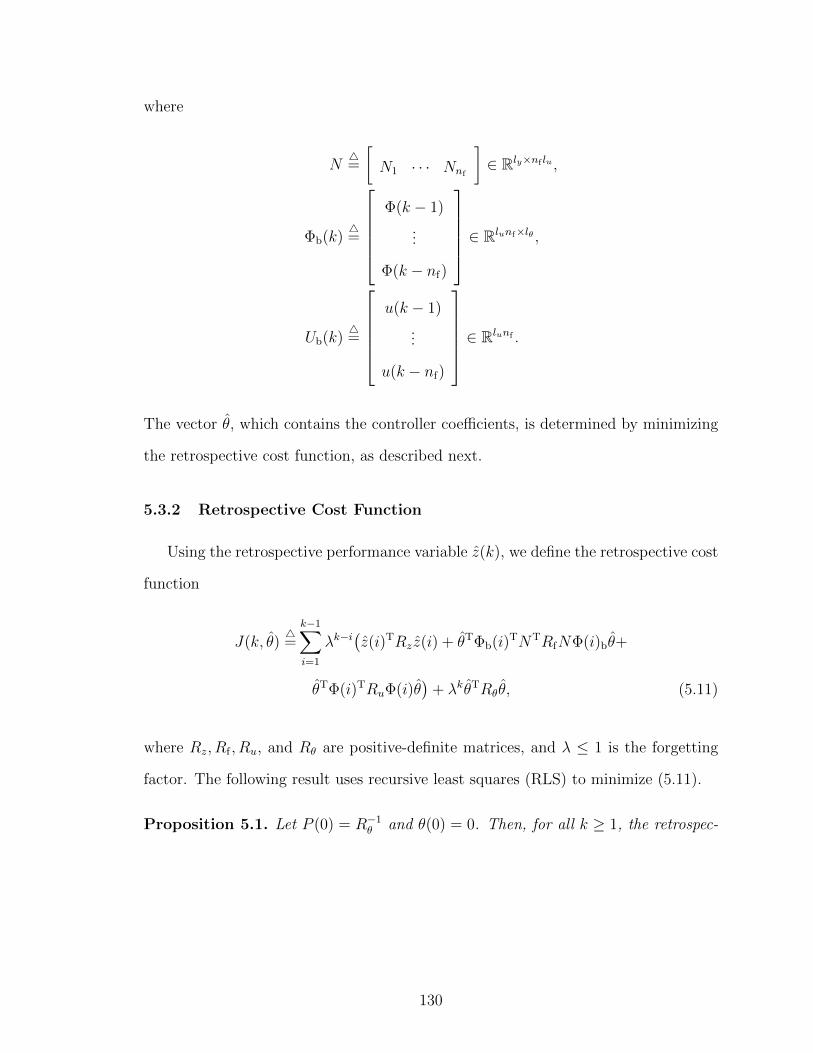
where
N4=
[N1 · · · Nnf
]∈ Rly×nf lu ,
Φb(k)4=
Φ(k − 1)
...
Φ(k − nf)
∈ Rlunf×lθ ,
Ub(k)4=
u(k − 1)
...
u(k − nf)
∈ Rlunf .
The vector θ, which contains the controller coefficients, is determined by minimizing
the retrospective cost function, as described next.
5.3.2 Retrospective Cost Function
Using the retrospective performance variable z(k), we define the retrospective cost
function
J(k, θ)4=
k−1∑i=1
λk−i(z(i)TRz z(i) + θTΦb(i)TNTRfNΦ(i)bθ+
θTΦ(i)TRuΦ(i)θ)
+ λkθTRθθ, (5.11)
where Rz, Rf , Ru, and Rθ are positive-definite matrices, and λ ≤ 1 is the forgetting
factor. The following result uses recursive least squares (RLS) to minimize (5.11).
Proposition 5.1. Let P (0) = R−1θ and θ(0) = 0. Then, for all k ≥ 1, the retrospec-
130

tive cost function (5.11) has a unique global minimizer θ(k), which is given by
θ(k) = θ(k − 1)− P (k)
NΦb(k − 1)
Φ(k − 1)
T Rz 0
0 Ru
·
NΦb(k − 1)θ(k − 1) + z(k − 1)−NUb(k − 1)
Φ(k − 1)θ(k − 1)
, (5.12)
P (k) = λ−1P (k − 1)− λ−1P (k − 1)
NΦb(k − 1)
Φ(k − 1)
T
· Γ(k)−1
NΦb(k − 1)
Φ(k − 1)
P (k − 1), (5.13)
where
Γ(k)4= λ
Rz 0
0 Ru
−1
+
NΦb(k − 1)
Φ(k − 1)
P (k − 1)
·
NΦb(k − 1)
Φ(k − 1)
T
. (5.14)
Furthermore, the control input at step k is given by
u(k) = Φ(k)θ(k). (5.15)
5.3.3 The Target Model Gf
The following result shows that the control u(k) is constrained to the subspace
spanned by the transposes of the coefficients of Gf .
Theorem 5.1. Let Rθ = βIlθ , Ru = γIlu and let θ(k) be given by (5.15). Let
131

Φ4= Ilu ⊗ φT, where φ ∈ Rlφ, and lφ
4= lθ/lu. Then, for all k ≥ 1,
Φθ(k) ∈ R
([NT
1 · · · NTnf
]). (5.16)
Proof. Note that
ΦAθ(k)θ(k) =k−1∑i=1
λk−iΦ(Φb(i)TNT(Rz +Rf)NΦb(i) + Φ(i)TγΦ(i)
)θ(k)+
λkβΦθ(k)
=k−1∑i=1
(λk−i
nf∑j=1
(Ilu ⊗ φT)(Ilu ⊗ φ(i− j))NTj
)(Rz +Rf)NΦb(i)θ(k)+
λk−i(Ilu ⊗ φT)(Ilu ⊗ φ(i))γΦ(i)θ(k) + λkβΦθ(k)
=k−1∑i=1
(λk−i
nf∑j=1
NTj φ
Tφ(i− j)
)(Rz +Rf)NΦb(i)θ(k)+
λk−iγφTφ(i)Φ(i)θ(k) + λkβΦθ(k)
=
[NT
1 · · · NTnf
] k−1∑i=1
λk−iΞ(i)(Rz +Rf)NΦb(i)θ(k) + Φ(k)θ(k),
where
Ξ(i)4=
φTφ(i− 1)⊗ Ilz
...
φTφ(i− nf)⊗ Ilz
,Φ(k)
4= Ilu ⊗ φ(k)T,
φ(k)4= M(k)φ,
M(k)4=
k−1∑i=1
λk−iγφ(i)φ(i)T + λkβIlφ .
132
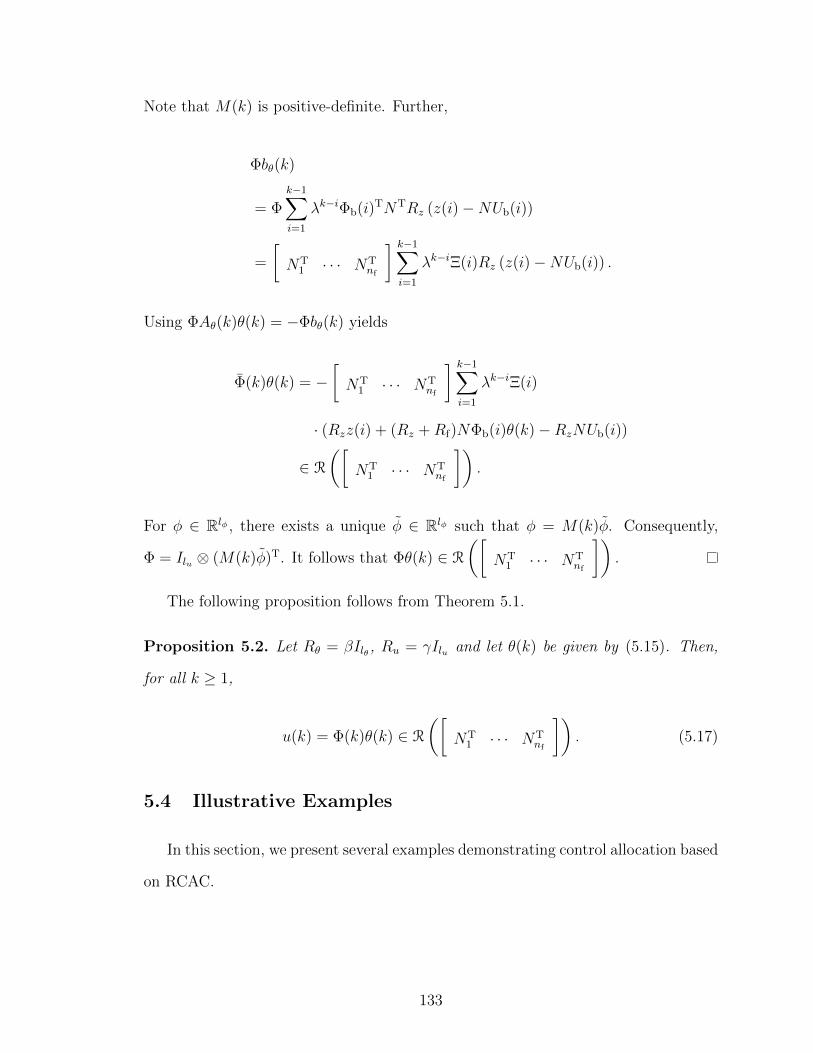
Note that M(k) is positive-definite. Further,
Φbθ(k)
= Φk−1∑i=1
λk−iΦb(i)TNTRz (z(i)−NUb(i))
=
[NT
1 · · · NTnf
] k−1∑i=1
λk−iΞ(i)Rz (z(i)−NUb(i)) .
Using ΦAθ(k)θ(k) = −Φbθ(k) yields
Φ(k)θ(k) = −[NT
1 · · · NTnf
] k−1∑i=1
λk−iΞ(i)
· (Rzz(i) + (Rz +Rf)NΦb(i)θ(k)−RzNUb(i))
∈ R
([NT
1 · · · NTnf
]).
For φ ∈ Rlφ , there exists a unique φ ∈ Rlφ such that φ = M(k)φ. Consequently,
Φ = Ilu ⊗ (M(k)φ)T. It follows that Φθ(k) ∈ R
([NT
1 · · · NTnf
]).
The following proposition follows from Theorem 5.1.
Proposition 5.2. Let Rθ = βIlθ , Ru = γIlu and let θ(k) be given by (5.15). Then,
for all k ≥ 1,
u(k) = Φ(k)θ(k) ∈ R
([NT
1 · · · NTnf
]). (5.17)
5.4 Illustrative Examples
In this section, we present several examples demonstrating control allocation based
on RCAC.
133
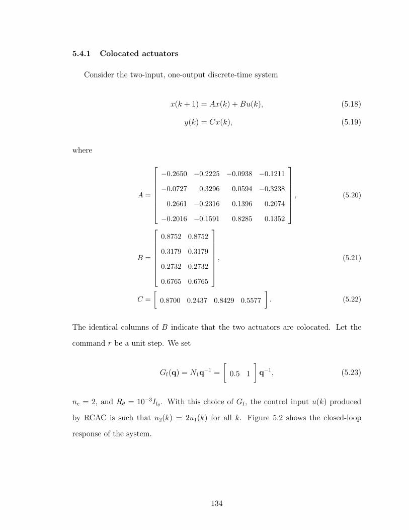
5.4.1 Colocated actuators
Consider the two-input, one-output discrete-time system
x(k + 1) = Ax(k) +Bu(k), (5.18)
y(k) = Cx(k), (5.19)
where
A =
−0.2650 −0.2225 −0.0938 −0.1211
−0.0727 0.3296 0.0594 −0.3238
0.2661 −0.2316 0.1396 0.2074
−0.2016 −0.1591 0.8285 0.1352
, (5.20)
B =
0.8752 0.8752
0.3179 0.3179
0.2732 0.2732
0.6765 0.6765
, (5.21)
C =
[0.8700 0.2437 0.8429 0.5577
]. (5.22)
The identical columns of B indicate that the two actuators are colocated. Let the
command r be a unit step. We set
Gf(q) = N1q−1 =
[0.5 1
]q−1, (5.23)
nc = 2, and Rθ = 10−3Ilθ . With this choice of Gf , the control input u(k) produced
by RCAC is such that u2(k) = 2u1(k) for all k. Figure 5.2 shows the closed-loop
response of the system.
134
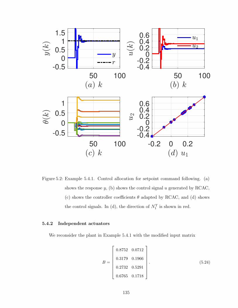
50 100
-0.5
0
0.5
1
1.5
50 100
-0.4-0.2
00.20.40.6
50 100
-0.5
0
0.5
1
-0.2 0 0.2
-0.4-0.2
00.20.40.6
Figure 5.2: Example 5.4.1. Control allocation for setpoint command following. (a)
shows the response y, (b) shows the control signal u generated by RCAC,
(c) shows the controller coefficients θ adapted by RCAC, and (d) shows
the control signals. In (d), the direction of NT1 is shown in red.
5.4.2 Independent actuators
We reconsider the plant in Example 5.4.1 with the modified input matrix
B =
0.8752 0.0712
0.3179 0.1966
0.2732 0.5291
0.6765 0.1718
. (5.24)
135

Let the command r be a unit step. We set
Gf(q) = N1q−1 =
[0.5 1
]q−1, (5.25)
nc = 2, and Rθ = 10−3Ilθ . With this choice of Gf , the control input produced by
RCAC is in the direction NT1 . Figure 5.3 shows the closed-loop response of the system.
50 100
0
0.5
1
50 100
0
0.2
0.4
0.6
50 100
-0.5
0
0.5
0 0.10.20.3
0
0.2
0.4
0.6
Figure 5.3: Example 5.4.2. Control allocation for setpoint command following. (a)
shows the response y, (b) shows the control signal u generated by RCAC,
(c) shows the controller coefficients θ adapted by RCAC, and (d) shows
the control signals. In (d), the direction of NT1 is shown in red.
136

5.4.3 Uncontrollable channels
We reconsider the plant in Example 5.4.1 with the modified input matrix
B =
[b1 b2
]=
0.8826 0.0984
0.5405 0.2135
0.0808 0.5128
0.3543 0.2059
. (5.26)
Note that (A, b1) and (A, b2) each have one uncontrollable mode, but (A,B) is con-
trollable. Hence, u1 and u2 must work together to achieve the control objective. Let
the command r be a unit step. We set
Gf(q) = N1q−1 =
[0.5 1
]q−1, (5.27)
nc = 2, and Rθ = 10−3Ilθ . With this choice of Gf , the control input produced by
RCAC is in the direction NT1 . Figure 5.4 shows the closed-loop response of the system.
137

50 100
0
0.5
1
50 100
0
0.2
0.4
0.6
50 100
-0.5
0
0.5
0 0.1 0.2 0.3
0
0.2
0.4
0.6
Figure 5.4: Example 5.4.3. Control allocation for setpoint command following. (a)
shows the response y, (b) shows the control signal u generated by RCAC,
(c) shows the controller coefficients θ adapted by RCAC, and (d) shows
the control signals. In (d), the direction of NT1 is shown in red.
5.5 Conclusions
This chapter presented a novel approach to control allocation for wide systems
within the context of retrospective cost adaptive control (RCAC). The approach is
based on the fact that the control input is constrained to the range of the transpose
of the target model. This technique was applied to illustrative examples.
The next chapter extends RCAC to asymptotically enforce auxiliary output con-
138

straints by formulating the auxiliary output constraints as conflicting commands.
139

CHAPTER 6
Output-Constrained Adaptive Control for Unstart
Prevention in a 2D Scramjet Combustor
6.1 Introduction
A supersonic combustion ramjet (scramjet) engine is an air-breathing propulsion
system that compresses and ignites a supersonic stream of air and generates thrust
by expelling high-energy gases through a nozzle without any moving parts. Scramjet
engines have high potential for high-speed transport, access to space, and payload
delivery. Although mechanically simple, the flow inside a scramjet engine, comprised
of pockets of subsonic regions and multiple shock structures, is extremely complex,
and is highly sensitive to external disturbances such as inlet mach number and angle
of attack of the leading ramp.
A major challenge in the operation of a scramjet is the problem of preventing
the scramjet from unstarting. The flow inside the scramjet can thermally choke
when sufficient heat is added in the combustor, resulting in a normal shock that
travels upstream, thereby destroying the shock structure and the supersonic flow.
Consequently, the thrust generated by the scramjet drops precipitously. Since it is
extremely difficult to re-establish stable supersonic flow structure quickly enough once
the engine has unstarted completely, unstart is usually fatal to the engine operation.
140

In addition to excessive heat addition, the scramjet engine can unstart because of
flow and structural perturbations.
In [97], unstart was prevented by constraining the hypersonic vehicle to remain
within a predefined flight envelope. In [98], a second-order linear, time-invariant
model relating the ramp angle and the shock train location was identified. A PID
controller was developed based on the identified model, and was applied to the high-
order model to shift the location of the shock train to prevent unstart. In [99],
a particle filter was used to estimate the state of a scramjet described by a one-
dimensional model, and a full-state-feedback control law was suggested to prevent
the scramjet from unstarting. As a result, the control altered the cycle length as well
as the burst length of the fuel flow based on the predicted future location of the shock
front computed using the filtered state. In [100], retrospective cost adaptive control
(RCAC) was used for unstart prevention in a 2D scramjet model with a single pressure
measurement near the combustor, however, the closed-loop response was oscillatory.
In the present work, RCAC is used to prevent unstart by enforcing auxiliary output
constraints.
RCAC is a direct discrete-time adaptive control algorithm that is applicable to sta-
bilization, command following, and disturbance rejection. RCAC minimizes a convex
cost function based on a performance variable, such as the thrust error, to optimize
the controller coefficients based on past control inputs and past measurements. The
retrospective cost minimized by RCAC is based on the retrospective performance,
which is defined using the target model Gf . The target model Gf reflects the qual-
itative response of the performance variable to the control input, which is usually
captured by the key dynamics features of the system to be controlled such as its rel-
ative degree, sign of the leading Markov parameter, and nonminimum-phase (NMP)
zeros, if any. As shown in [30], RCAC adapts the control law in order to match the
intercalated transfer function to the target model Gf .
141

RCAC was applied to the problem of possibly conflicting commands in an aircraft
to follow trim commands in [101]. The contribution of the present chapter is to
show that output constraints can be asymptotically enforced by casting them as
additional conflicting commands; these commands are conflicting in the sense that the
tradeoff necessitates a constraint violation. As in the case of conflicting commands,
the asymptotic response of the controlled system may not be able follow all of the
commands simultaneously, and thus RCAC automatically trades off the output error
and the constraint violation error. Although the constraint is violated, it is shown
that the asymptotic magnitude of the constraint violation can be reduced by varying
the tuning parameters in RCAC. By defining a conservative constraint, the required
constraint can be satisfied.
The chapter is organized as follows: in Section 6.2, the scramjet model used in this
chapter is presented; unstart and its characterization based on open-loop simulations
of the scramjet model is presented in Section 6.3. The control architecture for the
setpoint command following is presented in Section 6.4. In Section 6.5, RCAC is
extended to the problem of following conflicting setpoint commands. In Section 6.6,
RCAC is extended to the problem of preventing the scramjet from unstarting by
enforcing an auxiliary output constraint. Finally, the chapter is concluded in Section
6.7.
6.2 Scramjet Model
The scramjet engine considered in this work is based on the Hyshot-II geometry
[102] shown in Figure 6.1. The flow is modeled by coupled nonlinear partial differential
equations based on the assumption of inviscid flow along with a heat release model.
142
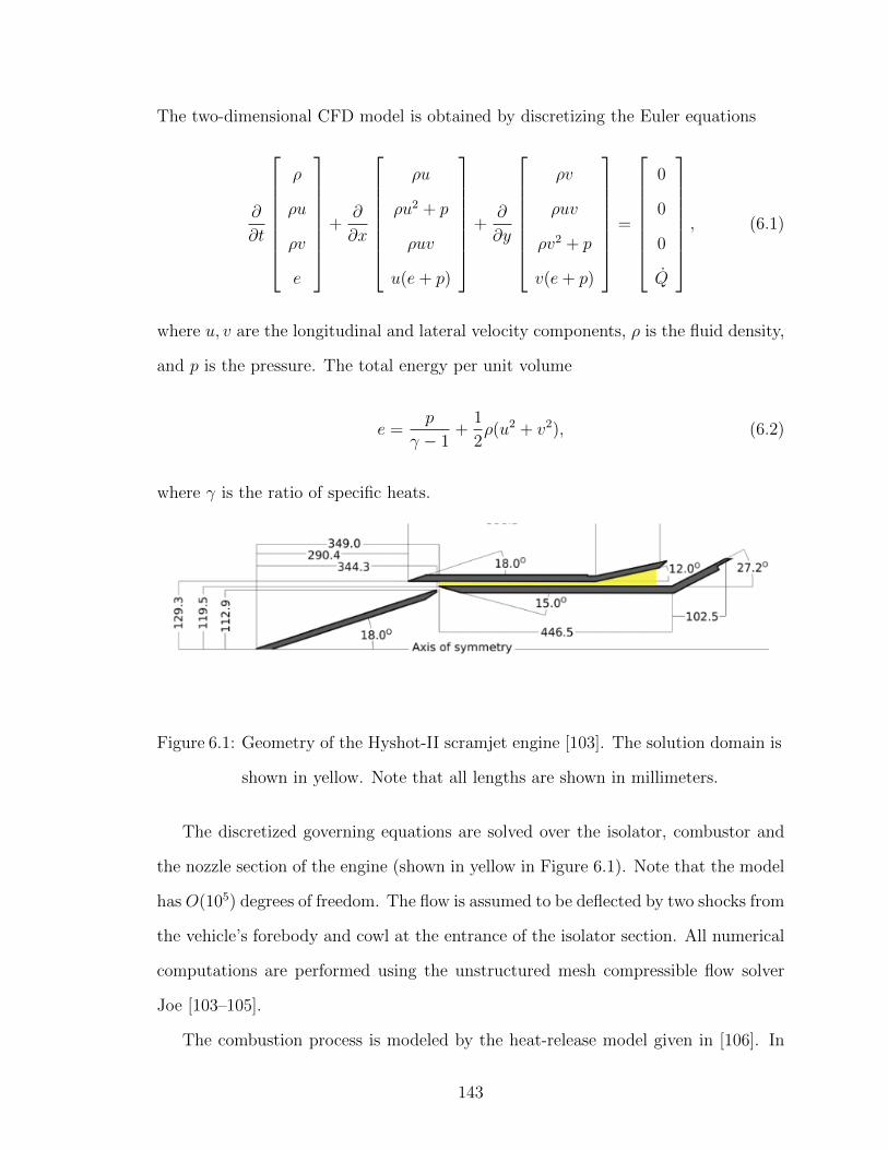
The two-dimensional CFD model is obtained by discretizing the Euler equations
∂
∂t
ρ
ρu
ρv
e
+
∂
∂x
ρu
ρu2 + p
ρuv
u(e+ p)
+
∂
∂y
ρv
ρuv
ρv2 + p
v(e+ p)
=
0
0
0
Q
, (6.1)
where u, v are the longitudinal and lateral velocity components, ρ is the fluid density,
and p is the pressure. The total energy per unit volume
e =p
γ − 1+
1
2ρ(u2 + v2), (6.2)
where γ is the ratio of specific heats.
Figure 6.1: Geometry of the Hyshot-II scramjet engine [103]. The solution domain is
shown in yellow. Note that all lengths are shown in millimeters.
The discretized governing equations are solved over the isolator, combustor and
the nozzle section of the engine (shown in yellow in Figure 6.1). Note that the model
has O(105) degrees of freedom. The flow is assumed to be deflected by two shocks from
the vehicle’s forebody and cowl at the entrance of the isolator section. All numerical
computations are performed using the unstructured mesh compressible flow solver
Joe [103–105].
The combustion process is modeled by the heat-release model given in [106]. In
143

particular, the source term Q is modeled by
Q = φfstHfmairη(x/Lc), (6.3)
η(x/Lc) = 1− e−(Cc(x−xc)/Lc)Dc, (6.4)
where xc < x < xc + Lc, φ is the fuel-air equivalence ratio, η is the heat-release
distribution function, and the numerical values of various parameters is given in Table
6.1. The thrust generated by the scramjet is computed by integrating the pressure
along the flow path, and is normalized and nondimensionalized by the free-stream
dynamic pressure and unit area. Finally, the heat addition, and thus the thrust is
controlled by varying the fuel-air equivalence ratio φ
Symbol Definition Nominal Value
fst Stoichiometric fuel/air ratio 0.028
Hf Fuel heating value (H2) 120 MJ/kg
xc Combustion ignition position 0.408 m
Lc Combustor length 0.368 m
Kc Fraction of completed combustion 0.95
Dc Shape parameter 0.75
Cc Shape parameter − log(1−Kc)1/Dc
Table 6.1: Summary of parameters used in the heat-release model (6.3), (6.4).
6.3 Unstart and Unstart detection
A major challenge in the operation of a scramjet is the need to prevent the scramjet
from unstarting. When sufficient heat is released in the combustor, usually by means
of too much fuel flow, the flow can thermally choke, resulting in a normal shock
that travels upstream, thereby destroying the shock structure and the supersonic
144

flow. Consequently, the thrust generated by the scramjet drops precipitously. This
is usually fatal to the engine operation since it is extremely difficult to establish
a stable supersonic flow structure quickly enough once the engine has unstarted. In
addition to excessive heat addition, a scramjet engine can unstart because of flow and
structural perturbations. Because of unstart, there is an upper limit on the thrust
that a scramjet engine can produce at a given operating condition. The maximum
asymptotic thrust that can be generated by the scramjet at a constant inlet Mach
number M0 is called the critical thrust at M0, and the constant equivalence ratio φ0
that corresponds to the critical thrust at M0 is called the critical equivalence ratio at
M0.
To characterize the onset of unstart, we simulate the scramjet without feedback
control for various fixed values of the equivalence ratio φ0 at various constant inlet
Mach numbers M0 for 3000 time steps. At each M0, if the applied equivalence ratio
is less than the critical equivalence ratio, the scramjet reaches a stable equilibrium
state and generates a constant thrust y0 at the end of the simulation. If, however,
the equivalence ratio is greater than the critical equivalence ratio, the state of the
scramjet starts diverging as it attempts to establish a stable subsonic flow inside the
scramjet, leading to a sharp loss of thrust. Figure 6.2(a) shows the asymptotic thrust
y0 for various values of constant equivalence ratios φ0 at various constant inlet Mach
numbers M0.
In [103], a functional defined based on the pressure profile on the upper wall of the
combustor is used to detect unstart. In [100], a single pressure measurement is used
to detect and prevent unstart. Since the shock structure shifts longitudinally as the
equivalence ratio is varied, the measured pressure can change sharply as the shock
moves across the pressure sensor. In the present work, the mean pm of the pressure
along the bottom wall near the combustor is used to detect unstart. Specifically, 20
pressure sensors located uniformly between x = 0.279 m and x = 0.294 m are used
145

to define the pressure metric pm. This sensor arrangement corresponds to pressure
measurements from 20 grid points in the simulation. Figure 6.2(b) shows the mean
pressure pm for various values of constant equivalence ratios φ0 at various constant
inlet Mach numbers M0. Note that the mean pressure metric pm increases abruptly
once the scramjet unstarts due to the presence of a normal shock wave. Hence, the
value of the metric pm can be used to constrain the control algorithm to prevent the
scramjet from unstarting.
0.25 0.3 0.35 0.4 0.45
0.26
0.28
0.3
0.32
0.34
0.36
(a) Steady state Thrust
0.25 0.3 0.35 0.4 0.45
0.3
0.35
0.4
0.45
0.5
0.55
(b) Pressure Metric
Figure 6.2: Critical thrust y0 and the pressure metric pm in the normal operating and
unstarting scramjet. The critical thrust at each value of M0 is shown with
a black circle.
6.4 Adaptive Setpoint Command Following
In this work, RCAC is used to optimize an infinite impulse response (IIR) con-
troller to follow setpoint thrust commands. The notation used for RCAC variables is
given in [100]. The scramjet is assumed to be operating in a steady state with the
equivalence ratio φ0 at the constant inlet Mach number M0. The thrust error, defined
as z(k)4= r(k) − y(k), where r(k) is the commanded value of the thrust and y(k) is
the generated thrust, is used to drive and optimize the controller Gc. The equivalence
ratio applied to the scramjet is φ(k) = φ0 + uc(k), where uc(k) is the output of Gc.
146

The control system architecture is shown in Figure 6.3.
- Gc
φ0
scramjet
M
uc φr z y
Figure 6.3: Scramjet command-following control system architecture. The controllerGc is updated by RCAC.
In [100], a feedback/feedforward controller structure is optimized using RCAC,
whereas, in this chapter, a feedback controller with an embedded integrator is opti-
mized. The embedded integrator ensures that uc(k) converges to the required constant
value as k →∞ and z(k)→ 0.
6.5 Adaptive Command Following with Conflicting Commands
Consider the SISO system
x(k + 1) = f(x(k), u(k)), (6.5)
y(k) = g(x(k), u(k)), (6.6)
where x(k) ∈ Rn is the state, u(k) ∈ R is the input, and y(k) ∈ R is the measured
output. The objective is to construct a control law such that y(k) − r(k) → 0 as
k →∞, where r(k) is the command.
As a first step in developing a strategy for enforcing constraints, we consider the
response of RCAC in the case of conflicting commands. In particular, we define the
147

performance variable
z(k)4=
y(k)− r1(k)
...
y(k)− rq(k)
∈ Rq, (6.7)
where r1(k), . . . , rq(k) ∈ R. If r1, . . . , rq are different signals, then the commands are
conflicting, that is, the output y(k) is simultaneously requested to follow different
commands. It is shown below that conflicting commands provide a technique for
asymptotically enforcing constraints.
Let
N1 =
N1,1
...
N1,q
, Rz = diag(Rz,1, . . . , Rz,q), (6.8)
where Rz,i > 0. Numerical examples show that, if limk→∞ z(k) exists, then
limk→∞
q∑j=1
N1,jRz,jzj(k) = 0. (6.9)
Consequently,
limk→∞
z(k) ∈ N(NT1 Rz), (6.10)
and thus,
limk→∞
y(k) =
∑qj=1Rz,jN1,jrj∑qj=1Rz,jN1,j
. (6.11)
Thus, by choosing N1, and Rz, (6.11) can be used to specify the tradeoff between
several conflicting commands. �
148
Example 6.1. Consider the spring-mass-damper system
mx+ cx+ kx = u, (6.12)
where x is the position of the particle with mass m = 1, the damping coefficient is
c = 5, the spring stiffness is k = 5, and u is the applied input. Let the measured
output be y(k) = x(kTs), where Ts = 0.01 sec is the sampling time.
The conflicting commands for the two-component performance variable (6.7) are
chosen to be the setpoints r1(k) = 1 and r2(k) = 2. RCAC is implemented with
N1 = [1 1]T, Rz = I2, Rθ = 102Ilθ , and λ = 0.999. Figure 6.4 shows the closed-loop
response of the spring-mass-damper system with conflicting commands, (a) shows the
measured output y(k), (b) shows the control u(k), (c) shows the output error z(k),
and (d) shows the coefficients of the controller optimized by RCAC.
Next, RCAC is implemented with N1 = [1 N1,2]T, Rz = diag(1, Rz,2), Rθ = 102Ilθ ,
and λ = 0.999, where N1,2 and Rz,2) are varied from 0.1 to 10. For each choice of
N1,2 and Rz,2, Figure 6.5 shows the asymptotic output y(k) the end of the simulation.
Note that the asymptotic output satisfies (6.11). �
149
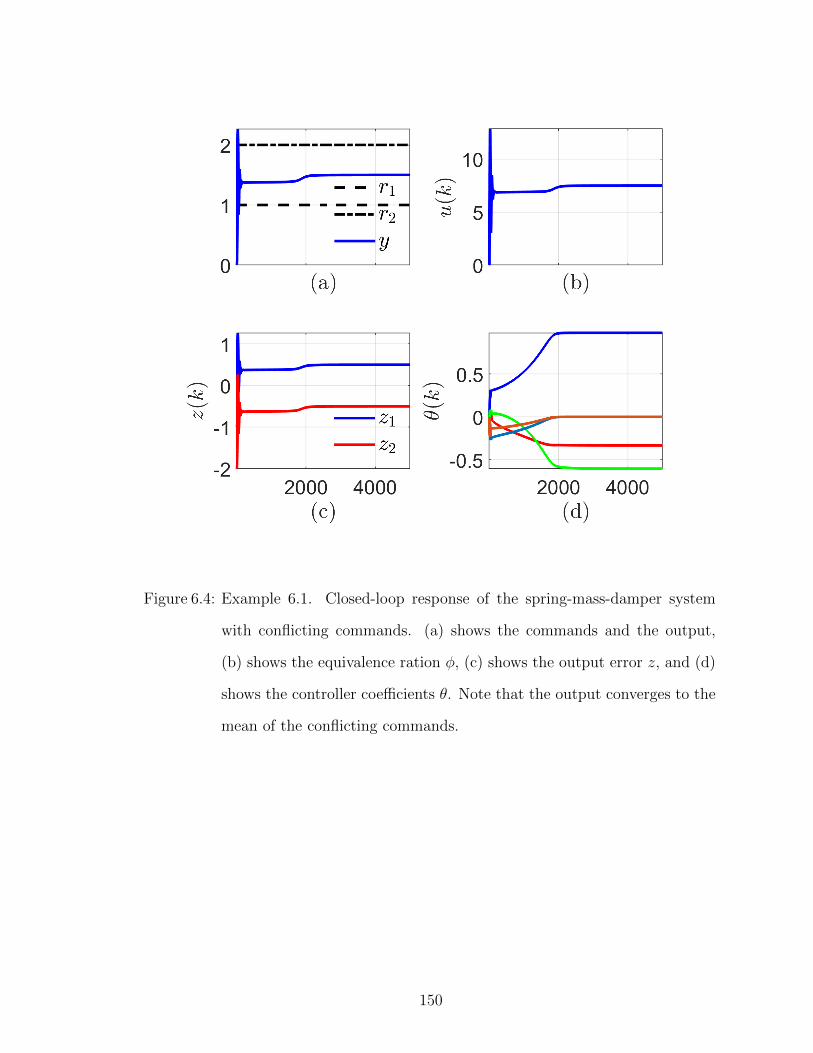
Figure 6.4: Example 6.1. Closed-loop response of the spring-mass-damper system
with conflicting commands. (a) shows the commands and the output,
(b) shows the equivalence ration φ, (c) shows the output error z, and (d)
shows the controller coefficients θ. Note that the output converges to the
mean of the conflicting commands.
150

10-1
100
101
10-1
100
101
1.1
1.2
1.3
1.4
1.5
1.6
1.7
1.8
Figure 6.5: Example 6.1. Asymptotic output of the spring-mass-damper system with
conflicting commands for various filter and performance weight choices.
Note that the asymptotic output satisfies (6.11).
Next, the closed-loop response of the scramjet to conflicting commands is consid-
ered. The conflicting commands are assumed to be less than the critical thrust at
the operating conditions. The scramjet is commanded to follow the step commands
r1(k) = 0.24 and r2(k) = 0.29 for all k > 0. At k = 0, the scramjet is assumed to be
operating in steady state with φ = 0.2 at the inlet Mach number M = 2.7. RCAC is
implemented with N1 = [0.1 0.1]T, λ = 0.9999, Rθ = 107I8, and Rz = I2. Figure 6.6
shows the closed-loop response of the scramjet to the conflicting commands. Note
that the asymptotic value of the generated thrust is in the middle of the commanded
151
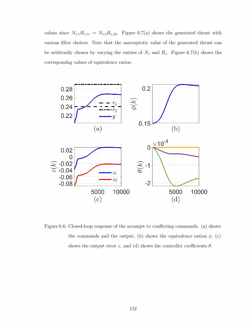
values since N1,1Rz,11 = N1,2Rz,22. Figure 6.7(a) shows the generated thrust with
various filter choices. Note that the assymptotic value of the generated thrust can
be arbitrarily chosen by varying the entries of N1 and Rz. Figure 6.7(b) shows the
correspondng values of equivalence ratios.
Figure 6.6: Closed-loop response of the scramjet to conflicting commands. (a) shows
the commands and the output, (b) shows the equivalence ration φ, (c)
shows the output error z, and (d) shows the controller coefficients θ.
152

(a) Thrust
(b) Equivalence ratio
Figure 6.7: Closed-loop response of the scramjet to conflicting commands for various
filter choices. (a) shows the commands and the output, and (b) shows
the equivalence ration φ.
153

6.6 Adaptive Command Following with Auxiliary Output
Constraints
Consider the system (6.5), (6.6), with auxiliary outputs
yc(k) = hc(x(k), u(k)), (6.13)
where yc(k) ∈ Rq is an auxiliary measured output to be constrained. Let r(k) be
the reference command. The objective is to construct a control law such that y(k)−
r(k) → 0 as k → ∞ while enforcing constraints of the form yc(k) ∈ Yc for all k ≥ 0,
where Yc ⊂ Rq. For all i = 1, . . . , q, the constraint on yci(k) is assumed to be given
by
ylci ≤ yci(k) ≤ yuci, (6.14)
where ylci, yuci are the lower and the upper constraint bounds.
Now, consider the performance variable
z(k)4=
R1d(yc1(k), ylc1, yuc1)
...
Rqd(ycq(k), ylcq, yucq)
y(k)− r(k)
, (6.15)
where Ri ≥ 0 and the two-sided constraint violation metric is defined by
d(yci(k), ylci, yuci)4=
yci(k)− yuci, yci(k) > yuci,
0, ylci ≤ yci(k) ≤ yuci,
yci(k)− ylci, yci(k) < ylci.
(6.16)
154
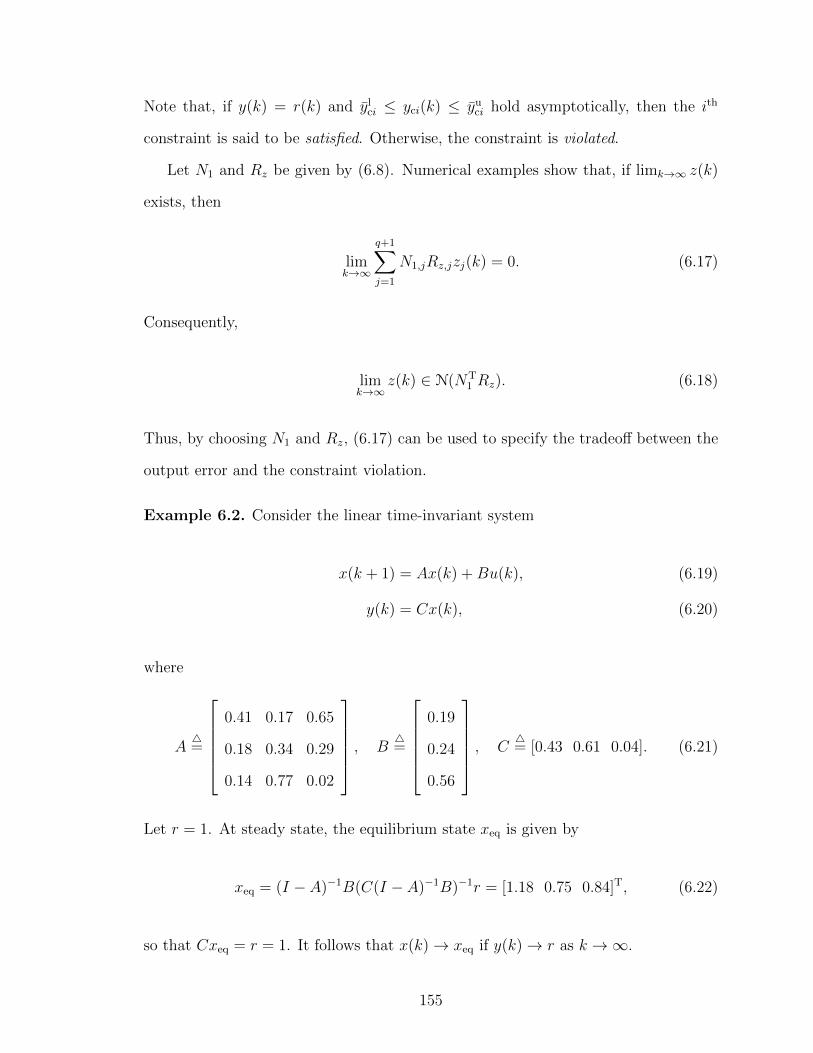
Note that, if y(k) = r(k) and ylci ≤ yci(k) ≤ yuci hold asymptotically, then the ith
constraint is said to be satisfied. Otherwise, the constraint is violated.
Let N1 and Rz be given by (6.8). Numerical examples show that, if limk→∞ z(k)
exists, then
limk→∞
q+1∑j=1
N1,jRz,jzj(k) = 0. (6.17)
Consequently,
limk→∞
z(k) ∈ N(NT1 Rz). (6.18)
Thus, by choosing N1 and Rz, (6.17) can be used to specify the tradeoff between the
output error and the constraint violation.
Example 6.2. Consider the linear time-invariant system
x(k + 1) = Ax(k) +Bu(k), (6.19)
y(k) = Cx(k), (6.20)
where
A4=
0.41 0.17 0.65
0.18 0.34 0.29
0.14 0.77 0.02
, B4=
0.19
0.24
0.56
, C4= [0.43 0.61 0.04]. (6.21)
Let r = 1. At steady state, the equilibrium state xeq is given by
xeq = (I − A)−1B(C(I − A)−1B)−1r = [1.18 0.75 0.84]T, (6.22)
so that Cxeq = r = 1. It follows that x(k)→ xeq if y(k)→ r as k →∞.
155

Consider the auxiliary output
yc(k) = x3(k), (6.23)
and consider the constraint given by yuc = 0.5. Thus, if r = 1, it follows from
(6.22) that the constraint is violated in the case where y(k)→ r as k →∞. RCAC is
implemented with N1 = [5 1]T, Rz = diag(10, 1), Rθ = 102Ilθ , R1 = 2, and λ = 0.999.
It follows from (6.17) that
limk→∞
100(yc(k)− yuc ) + y(k)− r = 0. (6.24)
Figure 6.8 shows the states and the constrained output of the system (6.19), (6.20).
Note that, asymptotically, the output error z2(k) = −0.4, and the constraint violation
metric yc(k)− yuc = 0.004 = −0.01z2(k) satisfy (6.24). �
156

1000 2000 3000 4000 5000
0
0.2
0.4
0.6
0.8
1
Figure 6.8: Example 6.2. Closed-loop response of the system (6.19), (6.20) with aux-
iliary output constraints. Note that the constraint is violated if the com-
mand is followed. Thus, asymptotically, the output error y(k)−r(k), and
the constraint violation metric yc(k)− yuc satisfy (6.24).
Next, the closed-loop response of the scramjet with the auxiliary output constraint
is considered, where the auxiliary output is the pressure metric pm defined in Section
6.3. Specifically, the constraint is given by
pm(k) ≤ 0.4. (6.25)
Note that pm = 0.4325 at the critical thrust M0 = 2.7. The scramjet is commanded
157

to follow the step command
r(k) =
0.32, k < 8000,
0.355, k ≥ 8000.
(6.26)
At k = 0, the scramjet is assumed to be operating in steady state with φ0 = 0.3 at
the inlet Mach number M = 2.7. RCAC is implemented with N1 = [1 1]T, Rz = I2, ,
Rθ = 107I8, R1 = 1, and λ = 0.9999.
For k < 8000, the commanded thrust is less than the critical thrust at the oper-
ating conditions, and thus the scramjet does not unstart and reaches a steady state.
Note that pm < 0.4 for k < 9000, and thus the constraint is satisfied. For k ≥ 8000,
the commanded thrust is greater than the critical thrust at the operating conditions,
thus the scramjet begins to unstart as the controller increases the equivalence ratio
to increase the generated thrust. However, the constraint eventually becomes active,
the scramjet converges to a steady state, and the output error and the constraint
violation metric converge to constant values based on the choice of N1, Rz, and R1.
Figure 6.9 shows the closed-loop response of the scramjet with auxiliary output
constraint, (a) shows the measured output y(k), (b) shows the equivalence ratio φ(k),
(c) shows the constraint violation metric z1(k) and the output error z2(k), and (d)
shows the coefficients of the controller optimized by RCAC.
158

Figure 6.9: Closed-loop response of the scramjet with the auxiliary output constraint.
(a) shows the commands and the output, (b) shows the equivalence ration
φ, (c) shows the output error z, and (d) shows the controller coefficients
θ.
6.7 Conclusions
In this chapter, retrospective cost adaptive control (RCAC) with auxiliary output
constraints was used to prevent a 2D scramjet combustor from unstarting. As a
first step towards enforcing output constraints, RCAC was applied to the problem
of following conflicting setpoint commands. The asymptotic response of the system
to the conflicting commands was shown to be directly related to the filter choice
159

and the performance weights in RCAC. Finally, RCAC was extended to implement
output constraints by defining the constraint violation metric and augmenting the
performance variable. The asymptotic response of the system and the asymptotic
constraint violation metric were shown to be directly related to the filter choice and
the performance weights in RCAC.
RCAC does not prevent the constraint from being violated. Instead, RCAC bal-
ances the several conflicting objectives by trading the cost between the output error
and the constraint violation metric. This tradeoff can be designed by the choice of
the filter choice and the performance weights in RCAC.
RCAC was implemented to follow conflicting commands and enforce auxiliary
output constraints in low-order linear systems to numerically explore the asymptotic
response. Finally, RCAC was applied to prevent the scramjet from unstarting by
using several pressure measurements as the auxiliary output.
The upper bound of the pressure metric used to prevent unstart used in this work
is based on open-loop simulations of the scramjet, which are chosen to be sufficiently
far from unstart.
160

CHAPTER 7
Conclusions and Future Work
This dissertation first presented retrospective cost parameter estimation algo-
rithm, which is an iterative, data-driven technique for estimating unknown parame-
ters in linear and nonlinear dynamical systems. Unlike the extended Kalman filter,
RCPE is gradient-free; unlike the unscented Kalman filter, RCPE is ensemble-free;
and unlike variational methods, RCPE is adjoint-free.
The parameter estimator system consisted of an adaptive integrator with an out-
put nonlinearity and a permutation. It was shown that to estimate multiple unknown
parameters, a permutation of the estimated paramters is required to correctly asso-
ciate each parameter estimate with the corresponding unknown parameter. The need
to select the permutation matrix is the price paid for not requiring gradient informa-
tion, an ensemble of models, or an adjoint model. In particular, it was shown that
for a choice filter coefficients that define the retrospective cost, there is exactly one
correct choice of permutation matrix. In fact, the parameter estimate diverges with
all other choices of the permutation matrix. In addition, it was shown that the RCPE
estimate is constrained to lie in a subspace defined by filter coefficients that define
the retrospective cost.
The potential usefulness of RCPE was demonstrated by application to the prob-
lem of estimating two unknown parameters in the Burgers equation, for which UKF
161

requires an ensemble of 207 models each with 101 states, requiring a total of 21,321
state updates. In contrast, RCPE required one model and testing of two permuta-
tions, which requires a total of 202 state updates (101 for each permutation).
Next, it was shown that RCPE can implemented with simultaneous optimization
of the filter coefficients. The resulting optimization problem is biquadratic and non-
convex, however it is convex in the filter coefficients and the parameter estimator
coefficients separately. Thus, an alternating convex search algorithm was used to
optimize the retrospective cost function. The extended RCPE is applied to the prob-
lem of estimating eddy diffusion coefficient in global ionosphere-thermosphere model
using the measurements of total electron content.
Several key issues remain unexplored in RCPE. First, the number of permutation
matrices that must be tested is potentially lµ!, which is prohibitive when lµ is large.
Fortunately, divergence of the parameter estimates can be used to rule out incorrect
permutation matrices. An online technique based on the performance metric may be
developed to determine the correct permutation matrices. Next, RCPE is based on
RLS with a constant, scalar forgetting factor, and the performance of RCPE tends to
be sensitive to the choice of λ. Variable-rate forgetting technique can be implemented
within RCPE to optimize the retrospective cost. Next, all of the examples consid-
ered in this dissertation involve asymptotically stable dynamics. Preliminary results
suggest that RCPE is effective for systems that are Lyapunov stable; however, in
this case, the performance of RCPE is sensitive to the weighting parameters. Better
understanding of this case is needed to mitigate the sensitivity.
Finally, this dissertation did not consider the problem of uncertainty propagation
in parameter estimation. It maybe possible to compute the parameter error covari-
ance in RCPE by using ensemble methods or analytical expressions. Furthermore,
methods such as unscented transformation, quadrature formulas maybe used to prop-
agate uncertainty separately. Finally, the independent propagation of state error and
162

parameter error covariance may be compared with Monte-Carlo based methods to
propagate uncertainty.
Next, this dissertation focused on forgetting in the context of recursive least
squares algorithm. Note that the minimizer of the retrospective cost in RCPE is
given by the RLS algorithm. It was shown that in the case where the excitation
is not persistent and forgetting factor is less than one, singular values of Pk cor-
responding to the singular vectors orthogonal to the information subspace diverge.
A data-dependent forgetting matrix scheme was developed to restrict forgetting to
the information subspace, and prevent Pk from diverging under lack of persistent
excitation.
Next, the dissertation focused on the problem of control allocation in wide systems
using RCAC. The approach is based on the fact that the control input is constrained to
the range of the transpose of the target model. This technique was demonstrated using
numerical examples. The illustrative examples that were considered were minimum
phase, and thus it was not necessary to account for the presence of NMP zeros.
Although NMP zeros are nongeneric in nonsquare plants, they arise generically in
square systems (with SISO plants as the special case 1× 1). It is thus of interest to
consider control allocation for NMP square systems. The challenge is thus to enforce
control allocation by choosing the filter coefficients to also account for the presence
of NMP zeros and simultaneously allowing the constraining the subspace defined by
the filter coefficients.
Finally, the dissertation presented a technique to asymptotically enforce auxil-
iary output constraints in RCAC. In particular, the problem of enforcing auxiliary
output constraints was formulated as a problem of following conflicting commands.
The asymptotic response of the system to the conflicting commands was shown to be
directly related to the filter choice and the performance weights in RCAC. Finally,
RCAC was extended to implement output constraints by defining the constraint vio-
163

lation metric and augmenting the performance variable. The asymptotic response of
the system and the asymptotic constraint violation metric were shown to be directly
related to the filter choice and the performance weights in RCAC.
It was shown that RCAC does not prevent the constraint from being violated.
Instead, RCAC balances the several conflicting objectives by trading the cost between
the output error and the constraint violation metric. This tradeoff can be designed
by the choice of the filter choice and the performance weights in RCAC.
The constraint violation metric was defined using a non-smooth nonlinear func-
tion. Future research should focus on using smooth nonlinear functions to construct
the constraint violation metric to improve the transient behaviour of the closed loop
system.
164

BIBLIOGRAPHY
165

BIBLIOGRAPHY
[1] L. Ljung, System Identification: Theory for the User, 2nd ed., ser. Prentice HallInformation and System Sciences Series. Prentice Hall, 1 1999.
[2] D. Morrision, “Methods for non-linear least squares problems and convergeneproofs, tracking programs and orbit determination,” in Proceedings of the JetPropulsion Laboratory Seminar, 1960, pp. 1–9.
[3] G. Booth, G. Box, M. Muller, and T. Peterson, “Forecasting by generalized re-gression methods, nonlinear estimation,(princeton-ibm),” Inter-national Busi-ness Machines Corporation, New York, 1959.
[4] D. W. Marquardt, “An Algorithm for Least-Squares Estimation ofNonlinear Parameters,” Journal of the Society for Industrial and AppliedMathematics, vol. 11, no. 2, pp. 431–441, 2005. [Online]. Available:http://www.siam.org/journals/ojsa.php
[5] T. S. Jaakkola and M. I. Jordan, “Bayesian Paramater Estimation viaVariational Methods,” Statistics and Computing, vol. 10, no. 10, pp. 25–37,2000. [Online]. Available: http://link.springer.com/10.1023/A:1008932416310
[6] R. L. Raffard, K. Amonlirdviman, J. D. Axelrod, and C. J. Tomlin, “An adjoint-based parameter identification algorithm applied to planar cell polarity signal-ing,” IEEE Transactions on Automatic Control, vol. 53, pp. 109–121, 2008.
[7] M. Eknes and G. Evensen, “Parameter estimation solving a weak constraintvariational formulation for an Ekman model,” Journal of Geophysical Research:Oceans, vol. 102, pp. 12 479–12 491, 1997.
[8] R. M. Errico, “What is an adjoint model?” Bulletin of the American Meteoro-logical Society, vol. 78, no. 11, pp. 2577–2592, 1997.
[9] I. M. Navon, “Practical and theoretical aspects of adjoint parameter estimationand identifiability in meteorology and oceanography,” Dynamics of atmospheresand oceans, vol. 27, no. 1-4, pp. 55–79, 1998.
[10] D. Kondrashov, C. Sun, and M. Ghil, “Data assimilation for a coupled ocean–atmosphere model. part ii: Parameter estimation,” Monthly Weather Review,vol. 136, no. 12, pp. 5062–5076, 2008.
166
[11] Y. Zhu and I. M. Navon, “Impact of parameter estimation on the performanceof the fsu global spectral model using its full-physics adjoint,” Monthly WeatherReview, vol. 127, no. 7, pp. 1497–1517, 1999.
[12] Z. Yang and J. M. Hamrick, “Variational inverse parameter estimation in a co-hesive sediment transport model: An adjoint approach,” Journal of GeophysicalResearch: Oceans, vol. 108, no. C2, 2003.
[13] G. Mercere, O. Prot, and J. A. Ramos, “Identification of parameterized gray-box state-space systems: From a black-box linear time-invariant representationto a structured one,” IEEE Transactions on Automatic Control, vol. 59, pp.2873–2885, 2014.
[14] C. Yu, L. Ljung, and M. Verhaegen, “Identification of structured state-spacemodels,” Automatica, vol. 90, pp. 54–61, 4 2018.
[15] A. Gelman, H. S. Stern, J. B. Carlin, D. B. Dunson, A. Vehtari, and D. B.Rubin, Bayesian data analysis. Chapman and Hall/CRC, 2013.
[16] S. Sarkka, Bayesian filtering and smoothing. Cambridge University Press,2013, vol. 3.
[17] H. White, “Maximum likelihood estimation of misspecified models,” Economet-rica: Journal of the Econometric Society, pp. 1–25, 1982.
[18] Z. Ghahramani and G. E. Hinton, “Parameter estimation for linear dynamicalsystems,” Technical Report CRG-TR-96-2, University of Totronto, Dept. ofComputer Science, Tech. Rep., 1996.
[19] R. Van der Merwe and E. A. Wan, “The square-root unscented Kalman fil-ter for state and parameter-estimation,” in Proceedings of IEEE InternationalConference on Acoustics, Speech, and Signal Processing, vol. 6. IEEE, 2001,pp. 3461–3464.
[20] L. Ljung, “Asymptotic behavior of the Extended Kalman filter as a parameterestimator for linear systems,” IEEE Transactions on Automatic Control, vol. 24,pp. 36–50, 2 1979.
[21] G. L. Plett, “Extended Kalman filtering for battery management systems ofLiPB-based HEV battery packs - Part 3. State and parameter estimation,”Journal of Power Sources, vol. 134, pp. 277–292, 2004.
[22] E. A. Wan and R. Van Der Merwe, “The unscented Kalman filter for nonlinearestimation,” in Adaptive Systems for Signal Processing, Communications, andControl Symposium. IEEE, 2000, pp. 153–158.
[23] G. Evensen, “The ensemble Kalman filter for combined state and parameterestimation,” IEEE Control Systems Magazine, vol. 29, pp. 83–104, 6 2009.
167

[24] H. Moradkhani, S. Sorooshian, H. V. Gupta, and P. R. Houser, “Dual state andparameter estimation of hydrological models using ensemble Kalman filter,”Advances in Water Resources, vol. 28, pp. 135–147, 2005.
[25] R. Madankan, P. Singla, T. Singh, and P. D. Scott, “Polynomial-chaos-basedBayesian approach for state and parameter estimations,” Journal of Guidance,Control, and Dynamics, vol. 36, pp. 1058–1074, 2013.
[26] J. L. Anderson, “An ensemble adjustment kalman filter for data assimilation,”Monthly weather review, vol. 129, no. 12, pp. 2884–2903, 2001.
[27] A. M. D’Amato, A. J. Ridley, and D. S. Bernstein, “Retrospective-cost-basedadaptive model refinement for the ionosphere and thermosphere,” StatisticalAnalysis and Data Mining, vol. 4, pp. 446–458, 8 2011.
[28] X. Zhou, D. S. Bernstein, J. L. Stein, and T. Ersal, “Battery state of healthmonitoring by estimation of side reaction current density via retrospective-cost subsystem identification,” Journal of Dynamic Systems, Measurement, andControl, vol. 139, p. 091007, 2017.
[29] A. Goel, K. Duraisamy, and D. S. Bernstein, “Parameter estimation in theburgers equation using retrospective-cost model refinement,” in Proc. Amer.Contr. Conf., Boston, MA, July 2016, pp. 6983–6988.
[30] Y. Rahman, A. Xie, and D. S. Bernstein, “Retrospective Cost Adaptive Control:Pole Placement, Frequency Response, and Connections with LQG Control,”IEEE Control System Magazine, vol. 37, pp. 28–69, 10 2017.
[31] T. S. Jaakkola and M. I. Jordan, “Bayesian parameter estimation via Varia-tional methods,” Statistics and Computing, vol. 10, pp. 25–37, 2000.
[32] R. Bellman and K. J. Astrom, “On structural identifiability,” Mathematicalbiosciences, vol. 7, no. 3-4, pp. 329–339, 1970.
[33] M. Grewal and K. Glover, “Identifiability of linear and nonlinear dynamicalsystems,” IEEE Trans. Autom. Contr., vol. 21, pp. 833–837, 12 1976.
[34] S. Stanhope, J. E. Rubin, and D. Swigon, “Identifiability of linear and linear-in-parameters dynamical systems from a single trajectory,” SIAM Journal onApplied Dynamical Systems, vol. 13, no. 4, pp. 1792–1815, 2014.
[35] I. M. Y. Mareels, R. R. Bitmead, M. Gevers, C. R. Johnson, R. L. Kosut, andM. A. Poubelle, “How exciting can a signal really be?” Systems & ControlLetters, vol. 8, pp. 197–204, 1987.
[36] J. C. Willems, P. Rapisarda, I. Markovsky, and B. L. De Moor, “A note onpersistency of excitation,” Systems & Control Letters, vol. 54, no. 4, pp. 325–329, 2005.
168

[37] M. R. S. M. R. S. Kulenovic and G. E. Ladas, Dynamics of second order ra-tional difference equations : with open problems and conjectures. Chapman &Hall/CRC, 2002.
[38] D. T. Blackstock, “Generalized burgers equation for plane waves,” The Journalof the Acoustical Society of America, vol. 77, no. 6, pp. 2050–2053, June 1985.
[39] R. Courant, K. Friedrichs, and H. Lewy, “On the partial difference equationsof mathematical physics,” IBM Journal of Research and Development, vol. 11,pp. 215–234, march 1967.
[40] K. F. Tapping, “The 10.7 cm solar radio flux (f10.7),” Space Weather, vol. 11,no. 7, pp. 394–406, 2013.
[41] L. Qian, A. G. Burns, S. C. Solomon, and W. Wang, “Annual/semiannualvariation of the ionosphere,” Geophys. Res. Lett., vol. 40, no. 10, pp. 1928–1933, 2013.
[42] T. Shimazaki, “Effective eddy diffusion coefficient and atmospheric compositionin the lower thermosphere,” J. Atmos. Terr. Physics, vol. 33, no. 9, pp. 1383–1401, 1971.
[43] P. M. Kintner, B. M. Ledvina, and E. R. de Paula, “Gps and ionosphericscintillations,” Space Weather, vol. 5, no. 9, 2007, s09003. [Online]. Available:http://dx.doi.org/10.1029/2006SW000260
[44] J. A. Klobuchar, “Ionospheric time-delay algorithm for single-frequency gpsusers,” IEEE Transactions on aerospace and electronic systems, no. 3, pp. 325–331, 1987.
[45] L. Liu, W. Wan, B. Ning, and M.-L. Zhang, “Climatology of the meantotal electron content derived from gps global ionospheric maps,” J. Geophys.Res.: Space Phys., vol. 114, no. A6, 2009, a06308. [Online]. Available:http://dx.doi.org/10.1029/2009JA014244
[46] N. Jakowski, C. Mayer, M. M. Hoque, and V. Wilken, “Total electron contentmodels and their use in ionosphere monitoring,” Radio Sci., vol. 46, no. 6,2011, rS0D18. [Online]. Available: http://dx.doi.org/10.1029/2010RS004620
[47] J. L. Lean, R. R. Meier, J. M. Picone, and J. T. Emmert, “Ionospherictotal electron content: Global and hemispheric climatology,” J. Geophys.Res.: Space Phys., vol. 116, no. A10, 2011, a10318. [Online]. Available:http://dx.doi.org/10.1029/2011JA016567
[48] L. Ciraolo and P. Spalla, “Comparison of ionospheric total electron content fromthe navy navigation satellite system and the gps,” Radio Sci., vol. 32, no. 3, pp.1071–1080, 1997. [Online]. Available: http://dx.doi.org/10.1029/97RS00425
169
[49] B. Tsurutani, A. Mannucci, B. Iijima, M. A. Abdu, J. H. A. Sobral,W. Gonzalez, F. Guarnieri, T. Tsuda, A. Saito, K. Yumoto, B. Fejer, T. J.Fuller-Rowell, J. Kozyra, J. C. Foster, A. Coster, and V. M. Vasyliunas, “Globaldayside ionospheric uplift and enhancement associated with interplanetaryelectric fields,” J. Geophys. Res.: Space Phys., vol. 109, no. A8, 2004, a08302.[Online]. Available: http://dx.doi.org/10.1029/2003JA010342
[50] J. Liu, B. Zhao, and L. Liu, “Time delay and duration of ionospheric totalelectron content responses to geomagnetic disturbances,” Annal. Geophys.,vol. 28, no. 3, pp. 795–805, 2010. [Online]. Available: https://www.ann-geophys.net/28/795/2010/
[51] E. G. Thomas, J. B. H. Baker, J. M. Ruohoniemi, A. J. Coster, andS.-R. Zhang, “The geomagnetic storm time response of gps total electroncontent in the north american sector,” J. Geophys. Res.: Space Phys.,vol. 121, no. 2, pp. 1744–1759, 2016, 2015JA022182. [Online]. Available:http://dx.doi.org/10.1002/2015JA022182
[52] A. G. Burrell, A. Goel, A. J. Ridley, and D. S. Bernstein, “Correction of the pho-toelectron heating efficiency within the global ionosphere-thermosphere modelusing retrospective cost model refinement,” J. Atmos. Solar-Terr. Phys., vol.124, pp. 30–38, 2015.
[53] A. M. Morozov, A. A. Ali, A. M. D’Amato, A. J. Ridley, S. L. Kukreja, andD. S. Bernstein, “Retrospective-cost-based model refinement for system emu-lation and subsystem identification,” in Proc. Conf. Dec. Contr., Orlando, FL,December 2011, pp. 2142–2147.
[54] A. A. Ali, A. Goel, A. J. Ridley, and D. S. Bernstein, “Retrospective-cost-basedadaptive input and state estimation for the ionosphere–thermosphere,” J. Aero.Inf. Sys., vol. 12, no. 12, pp. 767–783, 2015.
[55] Y. Rahman, A. Xie, and D. S. Bernstein, “Retrospective cost adaptive control:Pole placement, frequency response, and connections with lqg control,” IEEEContr. Sys. Mag., vol. 37, 2017, october.
[56] ——, “A Tutorial and Overview of Retrospective-Cost-Based Adaptive Con-trol,” Proc. Amer. Contr. Conf., pp. 3386–3409, July 2016.
[57] F. Sobolic and D. S. Bernstein, “Adaptive control with concurrent closed-loopidentification of time-varying nonminimum-phase zeros,” in Proc. Conf. Dec.Contr., Las Vegas, NV, December 2016, pp. 371–376.
[58] F. M. Sobolic, A. Goel, and D. S. Bernstein, “Retrospective cost adaptive con-trol using concurrent controller optimization and target-model identification,”in Proc. Amer. Contr. Conf., 2016, pp. 3416–3421.
170
[59] J. Gorski, F. Pfeuffer, and K. Klamroth, “Biconvex sets and optimization withbiconvex functions: a survey and extensions,” Math. Meth. Oper. Res., vol. 66,no. 3, pp. 373–407, 2007.
[60] A. Ridley, Y. Deng, and G. Toth, “The global ionosphere–thermosphere model,”J. Atmos. Solar-Terr. Phys., vol. 68, no. 8, pp. 839–864, 2006.
[61] A. E. Hedin, “Extension of the msis thermosphere model into the middle andlower atmosphere,” J. Geophys. Res.: Space Phys., vol. 96, no. A2, pp. 1159–1172, 1991.
[62] D. Bilitza, “International reference ionosphere 2000,” Radio Sci., vol. 36, no. 2,pp. 261–275, 2001.
[63] M.-J. Yu and D. S. Bernstein, “Retrospective cost subsystem estimation andsmoothing for linear systems with structured uncertainty,” Journal of AerospaceInformation Systems, pp. 1–19, October 2018.
[64] M. Grewal and K. Glover, “Identifiability of linear and nonlinear dynamicalsystems,” IEEE Trans. Autom. Contr., vol. 21, pp. 833–837, 12 1976.
[65] I. Y. Mareels and M. Gevers, “Persistence of excitation criteria,”in Proc. Conf. Dec. Contr, 1986, pp. 1933–1935. [Online]. Available:http://ieeexplore.ieee.org/document/4049134/
[66] I. M. Mareels and M. Gevers, “Persistency of excitation criteria forlinear, multivariable, time-varying systems,” Mathematics of Control, Signals,and Systems, vol. 1, no. 3, pp. 203–226, 1988. [Online]. Available:http://link.springer.com/10.1007/BF02551284
[67] B. D. O. Anderson, “Adaptive systems, lack of persistency of excitation andbursting phenomena,” Automatica, vol. 21, no. 3, pp. 247–258, 1985.
[68] G. Chowdhary and E. Johnson, “Concurrent learning for convergence in adap-tive control without persistency of excitation,” in Proc. Conf. Dec. Contr., 2010,pp. 3674–3679.
[69] G. Chowdhary, M. Muhlegg, and E. Johnson, “Exponential parameter andtracking error convergence guarantees for adaptive controllers without persis-tency of excitation,” Int. J. Contr., vol. 87, no. 8, pp. 1583–1603, 2014.
[70] S. Aranovskiy, A. Bobtsov, R. Ortega, and A. Pyrkin, “Performance enhance-ment of parameter estimators via dynamic regressor extension and mixing,”IEEE Trans. Autom. Contr., vol. 62, no. 7, pp. 3546–3550, 2017.
[71] P. Panda, J. M. Allred, S. Ramanathan, and K. Roy, “Learning to forget withadaptive synaptic plasticity in spiking neural networks,” J. Emerg. Selec. Top.Circ. Syst., vol. 8, no. 1, pp. 51–64, 2018.
171
[72] T. R. Fortescue, L. S. Kershenbaum, and B. E. Ydstie, “Implementation ofSelf-tuning Regulators with Variable Forgetting Factors,” Automatica, vol. 17,no. 6, pp. 831–835, 1981.
[73] C. Paleologu, J. Benesty, and C. Silviu, “A Robust Variable Forgetting FactorRecursive Least-Squares Algorithm for System Identification,” IEEE Sig. Proc.Lett., vol. 15, pp. 597–600, 2008.
[74] S.-H. Leung and C. F. So, “Gradient-Based Variable Forgetting Factor RLSAlgorithm in Time-Varying Environments,” IEEE Trans. Sig. Proc., vol. 53,no. 8, pp. 3141–3150, 2005.
[75] S. Song, J.-S. Lim, S. J. Baek, and K.-M. Sung, “Gauss Newton variable forget-ting factor recursive least squares for time varying parameter tracking,” Elec-tron. Lett., vol. 36, no. 11, pp. 988–990, 2000.
[76] D. J. Park, B. E. Jun, and K. J. H., “Fast tracking RLS algorithm using novelvariable forgetting factor with unity zone,” Electron. Lett., vol. 27, no. 23, pp.2150–2151, 1991.
[77] A. A. Ali, J. B. Hoagg, M. Mossberg, and D. S. Bernstein, “On the stability andconvergence of a sliding-window variable-regularization recursive-least-squaresalgorithm,” Int. J. Adapt. Control Signal Process., vol. 30, pp. 715–735, 2016.
[78] R. M. Canetti and M. D. Espana, “Convergence analysis of the least-squaresidentification algorithm with a variable forgetting factor for time-varying linearsystems,” Automatica, vol. 25, no. 4, pp. 609–612, 1989.
[79] R. Kulhavy, “Restricted exponential forgetting in real-time identification,” Au-tomatica, vol. 23, no. 5, pp. 589–600, 1987.
[80] R. Kulhavy and M. Karny, “Tracking of slowly varying parameters by direc-tional forgetting,” IFAC Proc., vol. 17, no. 2, pp. 687–692, 1984.
[81] G. Kreisselmeier, “Stabilized least-squares type adaptive identifiers,” IEEETrans. Autom. Contr., vol. 35, no. 3, pp. 306–310, 1990.
[82] L. Cao and H. Schwartz, “Directional forgetting algorithm basedon the decomposition of the information matrix,” Automat-ica, vol. 36, no. 11, pp. 1725–1731, 2000. [Online]. Available:https://www.sciencedirect.com/science/article/pii/S0005109800000935
[83] G. Kubin, “Stabilization of the RLS algorithm in the absence of persistentexcitation,” in Proc. Int. Conf. Acoustics, Speech, Signal Processing, 1988, pp.1369–1372.
[84] S. Bittanti, P. Bolzern, and M. Campi, “Convergence and exponential conver-gence of identification algorithms with directional forgetting factor,” Automat-ica, vol. 26, no. 5, pp. 929–932, 1990.
172

[85] ——, “Exponential convergence of a modified directional forgetting identifica-tion algorithm,” Systems & Control Letters, vol. 14, no. 2, pp. 131–137, 1990.
[86] S. A. U. Islam and D. S. Bernstein, “Recursive Least Squares for Real-TimeImplementation,” Contr. Sys. Mag., vol. 39, June 2019.
[87] R. M. Johnstone, C. R. Johnson, R. R. Bitmead, and B. D. O. Anderson,“Exponential convergence of recursive least squares with exponential forgettingfactor,” in Proc. Conf. Dec. Contr., 1982, pp. 994–997.
[88] J. Benesty and T. Gansler, “New Insights into the RLS Algorithm,”Eurasip Jour. App. Sig. Proc., no. 3, pp. 331–339, 2004. [Online]. Available:https://link.springer.com/content/pdf/10.1155%2FS1110865704310188.pdf
[89] W. M. Haddad and V. Chellaboina, Nonlinear Dynamical Systems and Control:A Lyapunov-based Approach. Princeton University Press, 2008. [Online].Available: https://press.princeton.edu/titles/8700.html
[90] O. Harkegard and S. T. Glad, “Resolving actuator redundancy–optimal controlvs. control allocation,” Automatica, vol. 41, pp. 137–144, 2005.
[91] T. A. Johansen and T. I. Fossen, “Control allocationA survey,” Automatica,vol. 49, pp. 1087–1103, 2013.
[92] W. C. Durham, “Constrained Control Allocation,” AIAA J. Guid. Contr. Dyn.,vol. 16, pp. 717–725, 1993.
[93] D. F. Enns, “Control Allocation Approaches,” in Proc. Guid. Nav. Contr. Conf.,Boston, August 1998, AIAA-98-4109.
[94] J. J. Burken, P. Lu, Z. Wu, and C. Bahm, “Two Reconfigurable Flight-ControlDesign Methods: Robust Servomechanism and Control Allocation,” AIAA J.Guid. Contr. Dyn., vol. 24, pp. 482–493, 2001.
[95] M. Bodson, “Evaluation of Optimization Methods for Control Allocation,”AIAA J. Guid. Contr. Dyn., vol. 25, pp. 703–711, 2002.
[96] Y. Rahman, A. Xie, and D. S. Bernstein, “Retrospective Cost Adaptive Control:Pole Placement, Frequency Response, and Connections with LQG Control,”IEEE Contr. Sys. Mag., vol. 37, pp. 28–69, October 2017.
[97] M. Brocanelli, Y. Gunbatar, A. Serrani, and M. A. Bolender, “Robust Controlfor Unstart Recovery in Hypersonic Vehicles,” in AIAA Guidance, Navigation,and Control Conference, ser. Guidance, Navigation, and Control and Co-locatedConferences. Reston, Virigina: American Institute of Aeronautics and Astro-nautics, 8 2012.
[98] J. R. Hutzel, Scramjet Isolator Modeling and Control. Air Force Institute ofTechnology: ProQuest Dissertations Publishing, 2011, uMI number 3481728.
173

[99] N. West, G. Papanicolaou, P. Glynn, and G. Iaccarino, “A Numerical Study ofFiltering and Control for Scramjet Engine Flow,” in 20th AIAA ComputationalFluid Dynamics Conference, ser. Fluid Dynamics and Co-located Conferences.American Institute of Aeronautics and Astronautics, 6 2011.
[100] A. Goel, K. Duraisamy, and D. S. Bernstein, “Retrospective Cost AdaptiveControl of Unstart in a Model Scramjet Combustor,” AIAA Journal, vol. 56,no. 3, pp. 1085–1096, 2018.
[101] M.-J. Yu, E. M. Atkins, I. Kolmanovsky, and D. Bernstein, “Trim-CommandedAdaptive Control for Waypoint-Defined Trajectory Following,” in AIAA Guid-ance, Navigation, and Control (GNC) Conference. Reston, Virginia: AmericanInstitute of Aeronautics and Astronautics, aug 2013.
[102] M. K. Smart, N. E. Hass, and A. Paull, “Flight Data Analysis of the HyShot2 Scramjet Flight Experiment,” AIAA Journal, vol. 44, no. 10, pp. 2366–2375,10 2006.
[103] Q. Wang, K. Duraisamy, J. J. Alonso, and G. Iaccarino, “Risk assessment ofscramjet unstart using adjoint-based sampling methods,” AIAA journal, vol. 50,no. 3, pp. 581–592, 2012.
[104] R. Pecnik, V. E. Terrapon, F. Ham, G. Iaccarino, and H. Pitsch, “Reynolds-averaged Navier-Stokes simulations of the HyShot II scramjet,” AIAA journal,vol. 50, no. 8, pp. 1717–1732, 2012.
[105] K. Duraisamy and J. Alonso, “Adjoint based techniques for uncertainty quan-tification in turbulent flows with combustion,” in 42nd AIAA Fluid DynamicsConference and Exhibit, 2012, p. 2711.
[106] C. Doolan and R. Boyce, “A Quasi-One-Dimensional Mixing and CombustionCode for Trajectory Optimisation and Design Studies,” in AIAA InternationalSpace Planes and Hypersonic Systems and Technologies Conference, no. AIAA2008-2603, Dayton, Ohio, 2008, pp. 898–907.
174


![Prediction performance of linear models and gradient ......2021/08/02 · linear (GBLUP, BayesB and elastic net [ENET]) 18 methods to a non-parametric tree-based ensemble (gradient](https://img.pdfslide.us/doc/110x75/61415a9ca2f84929c304564e/prediction-performance-of-linear-models-and-gradient-20210802-linear.jpg)