Gradient based fuzzy c-means algorithm - FIU Digital Commons

Florida International UniversityFIU Digital Commons

FIU Electronic Theses and Dissertations University Graduate School

7-7-1994

Gradient based fuzzy c-means algorithmIssam J. DagherFlorida International University

DOI: 10.25148/etd.FI14061586Follow this and additional works at: https://digitalcommons.fiu.edu/etd

Part of the Electrical and Computer Engineering Commons

This work is brought to you for free and open access by the University Graduate School at FIU Digital Commons. It has been accepted for inclusion inFIU Electronic Theses and Dissertations by an authorized administrator of FIU Digital Commons. For more information, please contact [email protected].

Recommended CitationDagher, Issam J., "Gradient based fuzzy c-means algorithm" (1994). FIU Electronic Theses and Dissertations. 2652.https://digitalcommons.fiu.edu/etd/2652

https://digitalcommons.fiu.edu/?utm_source=digitalcommons.fiu.edu%2Fetd%2F2652&utm_medium=PDF&utm_campaign=PDFCoverPages

https://digitalcommons.fiu.edu/etd?utm_source=digitalcommons.fiu.edu%2Fetd%2F2652&utm_medium=PDF&utm_campaign=PDFCoverPages

https://digitalcommons.fiu.edu/ugs?utm_source=digitalcommons.fiu.edu%2Fetd%2F2652&utm_medium=PDF&utm_campaign=PDFCoverPages

https://digitalcommons.fiu.edu/etd?utm_source=digitalcommons.fiu.edu%2Fetd%2F2652&utm_medium=PDF&utm_campaign=PDFCoverPages

http://network.bepress.com/hgg/discipline/266?utm_source=digitalcommons.fiu.edu%2Fetd%2F2652&utm_medium=PDF&utm_campaign=PDFCoverPages

https://digitalcommons.fiu.edu/etd/2652?utm_source=digitalcommons.fiu.edu%2Fetd%2F2652&utm_medium=PDF&utm_campaign=PDFCoverPages

mailto:[email protected]

FLORIDA IN TERN A TIO N A L U N IV ER SITY

M iam i, F lorida

G radient Based Fuzzy c-means A lgorithm

A thesis subm itted in p artia l satisfaction of th e

requirem ents for th e degree of

M A STER OF SCIEN CE

IN

ELECTRICA L E N G IN E ER IN G

by

Issam J. D agher

1994

To: Dean Gordon R. HopkinsCollege of Engineering and Design

This thesis, written by Issam J. Dagher, and entitled GRADIENT BASED FUZZY C-MEANS ALGORITHM, having been approved in respect to style and intellectual content, is referred to you for judgement.

We have read this thesis and recommend th a t it be approved.

Malek Adjouadi

Malcolm Heimer

Dong C. Park, M ajor Professor

Date of Defense: July 7, 1994.

The thesis of Issam J. Dagher is approved.

Dean Gordon R. Hopkins College of Engineering and Design

Dr. Richard L. Campbell Dean of Graduate Studies

Florida International University, 1994

ACKNOWLEDGEMENTS

I would like to thank the members of my committee for all their

support and constructive criticism in the development of my thesis. I

also wish to give thanks to the members of the Intelligent Computing

Research Laboratory for their timely comments and overall help.

I also would like to give a special thanks to my major professor, Dr.

Park, for his extended support in my research and thesis development,

to my parents for their good example.

The research described in this thesis was supported in part by the

National Science Foundation grant CDA-9313624 with the Center for

Advanced Technology and Education.

A BSTR A C T OF THE THESIS

G R A D IEN T BASED FUZZY C-M EANS ALGORITHM

by

Issam J. Dagher

Florida International University, 1994

Professor Dong C. Park, Major Professor

A clustering algorithm based on the Fuzzy c-means algorithm

(FCM) and the gradient descent method is presented. In the FCM, the

minimization process of the objective function is proceeded by solving

two equations alternatively in an iterative fashion. Each iteration

requires the use of all the data at once. In our proposed approach one

datum is presented at a time to the network and the minimization is

proceeded using the gradient descent method. Compared to FCM,the

experimental results show that our algorithm is very competitive in

terms of speed and stability of convergence for large number of data.

Table o f C ontents

1 In troduction 1

2 C lustering Techniques 4

2.1 Crisp clustering.............................................................. 6

2.2 Fuzzy clustering ........................................................... 7

3 Decision Functions - O ptim ization 9

3.1 Steepest descent m ethod............................................... 10

3.2 Steepest descent algorithm............................................ 11

4 Decision Function For H ard C lustering - Kohonen N et

work 15

4.1 Kohonen Network ......................................................... 16

4.2 Winner-Takes-All ......................................................... 18

5 Decision Function For Fuzzy C lustering - Fuzzy C-

M eans A lgorithm 19

V

5.1 Hard vs.Fuzzy partitions................................................ 19

5.2 Fuzzy c-means partitions................................................ 22

5.2.1 Minimization of Jm(/z, v ) .................................... 22

5.2.2 Fuzzy c-means a lg o rith m ................................. 23

6 Gradient Based Fuzzy C-M eans Algorithm 24

6.1 Derivation of the algo rithm .......................................... 24

6.2 Comparison between FCM and GBFCM ..................... 25

6.3 GBFCM algorithm ......................................................... 26

6.4 Improving the speed of convergence.............................. 27

6.4.1 Moving the centers to their transitional directions 27

6.4.2 Decreasing the learning s tep .............................. 27

6.5 Convergence of GBFCM vs. F C M .............................. 28

7 A pplication Of GBFCM To Image Segm entation 35

7.1 Detection of e d g e s ......................................................... 35

7.2 Thresholding................................................................. 37

7.3 Region Splitting and M erging....................................... 39

7.4 Unsupervised image segmentation................................. 39

7.4.1 Implementation................................................... 40

7.4.2 Results ............................................................... 41

vi

7.5 Stopping GBFCM and FCM at different iterations . . 48

7.6 Discussion........................................................................ 53

8 Application O f GBFCM To Regression A nalysis 54

8.1 Least squares estimation of the p a ram ete rs ............... 54

8.2 Unsupervised regression an a ly s is ................................. 55

8.3 Unsupervised learning - Objective fu n c tio n ............... 56

8.3.1 Objective function ............................................. 56

8.3.2 Estimating the parameters of the system . . . . 57

8.3.3 Results ............................................................... 58

9 A pplication O f GBFCM To R eduction o f features of

the Fourier transform of the EMG signal 61

9.1 Signal classification and recognition.............................. 62

9.2 Neural networks as a classifier .................................... 62

9.3 Unsupervised learn in g ................................................... 63

9.4 Results.............................................................................. 70

10 Conclusions 71

10.1 Future Work ................................................................ 71

List o f Figures

2.1 Unsupervised learning..................................................... 5

2.2 Supervised learning.......................................................... 5

3.1 Example of an objective function................................... 13

3.2 Projection of the objective function............................... 13

3.3 Proceedings of the Gradient Descent method............... 14

4.1 Kohonen network............................................................. 17

5.1 Membership grades for 3 clusters................................... 21

6.1 Input datal....................................................................... 29

6.2 Error vs. iteration for 2 clusters for datal.................... 29



6.5 Input d a ta 2 .................................................................... 31

6.6 Error vs. iteration for 2 clusters for.data2.................... 31

6.7 Error vs. iteration for 3 clusters for.data2.................... 32

viii

6.8 Error vs. iteration for 4 clusters for data2....................... 32

6.9 Input d a ta 3 ...................................................................... 33

6.10 Error vs. iteration for 2 clusters for data3..................... 33



7.1 Image of the Japanese flag............................................ 38

7.2 Histogram of the Japanese flag....................................... 38

7.3 Imagel of Lenna............................................................... 42

7.4 2-level segmentation of imagel.............................. 42



7.7 Image2 of a walkway........................................................ 44

7.8 2-level segmentation of image2.............................. 44



7.11 Image3 of a scene.............................................................. 46




7.15 Mean vs. standard deviation for the Lenna image. . . 48

ix

7.16 Error vs. iteration for 4 clusters...................................... 48

7.17 FCM 4 clusters - 2 iterations........................................... 49

7.18 GBFCM 4 clusters - 2 iterations..................................... 49







8.1 Input d ata l......................................................................... 58

8.2 2 clusters - 2 curves for data l.......................................... 58

8.3 Input data2......................................................................... 59

8.4 2 clusters - 2 curves for data2.......................................... 59

8.5 Input data3......................................................................... 60

8.6 3 clusters - 3 curves for data3.......................................... 60

9.1 Signal classification............................................................ 62

9.2 Neural network as a classifier........................................... 64

9.3 Reduction of features using GBFCM algorithm............ 64

9.4 Pattern 1 of the resting position...................................... 65

9.5 Pattern 2 of the resting position...................................... 65

X

9.6 Pattern 1 of the.mid position......................................... 66

9.7 Pattern 2 of the.mid position......................................... 66

9.8 Pattern 1 of the max position......................................... 67

9.9 Pattern 2 of the max position......................................... 67

9.10 6-point patterns for the min position............................ 68

9.11 6-point patterns for the mid position............................ 68

9.12 6-point patterns for the max position........................... 69

xi

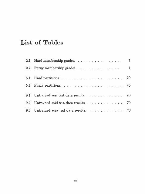
List o f Tables

2.1 Hard membership grades.................................................. 7

2.2 Fuzzy membership grades................................................. 7

5.1 Hard partitions.................................................................. 20

5.2 Fuzzy partitions................................................................. 20

9.1 Untrained rest test data results....................................... 70

9.2 Untrained mid test data results....................................... 70

9.3 Untrained max test data results....................................... 70

xii

Chapter 1

Introduction

The objective of clustering algorithms is the grouping of similar

objects and separating of dissimilar ones [1]. Kohonen [2] introduced

a network where the learning is based on the Winner-Takes-All rule.

It is based on the premise that one of the output neurons has the

maximum response due to an input. Only one winner is declared

(membership of 1) and all others are loosers (memberships of 0).

In 1973, Dunn [3] introduced a generalization of the Winner-Takes-

All rule. He combined Zadeh’s set concept with the criterion approach

to clustering. The membership grade is spread over {0, •••,!} which

will be able to “signal the presence or absence of Well-Separated Clus

ters” . He derived the necessary conditions for minimizing an objective

function. He called this method fuzzy ISODATA. A generalization of

the fuzzy ISODATA is done by Bezdek [4]. Bezdek defined a family

of objective functions {Jm, 1 < m < oo}, and established a conver-

l

gence theorem for that family. Windham presented a cluster validity

for the FCM algorithm [5]. He obtained a measure by computing the

ratio of the smallest membership to the largest one and transforming

this ratio into a probability function. In [6], an unsupervised fuzzy

clustering algorithm had been presented. The algorithm located the

regions where the data have low degree of memberships, and tried to

augment the number of clusters according to these regions.

In this thesis, we present a new algorithm called Gradient Based

FCM (GBFCM) which combines the characteristics of Kohonen net

work (presenting one datum at a time and applying the gradient de

scent method) and the FCM algorithm ( continuous values of the

membership grades in the range {0, “ *,1} ). In Chapter 2, differ

ent clustering techniques are presented. In Chapter 3, the minimiza

tion procedure (gradient descent method) is presented. The decision

functions for hard and fuzzy clustering are presented respectively in

Chapters 4 and 5. A derivation of the GBFCM algorithm is pre

sented in Chapter 6 establishing a comparison between FCM and

GBFCM and showing the pseudocode of the algorithm. Chapters

7,8,and 9 contain the results of applying GBFCM on image segmen

tation,regression analysis, and reduction of features of the Fourier

2

transform of the EMG signal. We conclude in Chapter 10 with a

short discussion about the algorithm and how it could be improved.

3

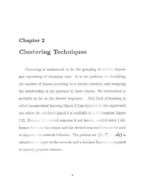
C lustering Techniques

C h ap ter 2

Clustering is understood to be the grouping of similar objects

and seperating of dissimilar ones. It is the problem of identifying

the number of classes according to a certain criterion, and assigning

the membership of the patterns in these classes. No information is

available as far as the desired responses . This kind of learning is

called unsupervised learning (figure 2.1)as opposed to the supervised

one where the teacher’s signal d is available at each iteration (figure

2.2). Because the desired response is not known, explicit error ( dif

ference between the output and the desired response) cannot be used

to improve the network behavior. The pattern set {afi, #2, . . . , is

submitted as input to the network and a decision function is required

to identify possible clusters .

4

5

Depending on the choice of this decision function, two approaches

can be used:

• Crisp clustering.

• Fuzzy clustering.

2.1 Crisp clustering

If X is a finite set, a family {A,*; 1 < i < c} is a crisp c-clusters of

X if:

U Ai = X (2.1)

A{ n A j = 0 for i ^ j (2.2)

The membership functions are:

~ { p ; « Z t A i (23)

S Ali(xk) = 1 for 1 < i < c and 1 < k < n (2.4)f=i

0 < T,M**) < n (2-5)*=iwhere n is the number of data, and c is the number of clusters.

For example :

X = {#1, x2, #3} n = 3

for 2 clusters c = 2 :

Exam ple 1:

exl xl x2 x3A1 1 1 0A2 0 0 1

Table 2.1: Hard membership grades.

The table shows that re 1 and x2 are in the class (cluster) A1 and x3

is in A2.

2.2 Fuzzy clustering

A fuzzy clustering is defined by the following properties of the

membership function:

0, •••,!} (2.6)

E f t W = l (2.7)<=1

0 < Z M xt) < n (2.8)k= 1

Exam ple 2:

ex3 xl x2 x3A1 .91 .58 .13A2 .09 .42 .87

Table 2.2: Fuzzy membership grades.

From the table, the following conclusions can be drawn:

7

• x l is most likely in A l.

• x3 is most likely in A2.

• x2 combines both properties of A l and A2 even though it does

not belong completely to one of the groups.

8

D ecision Functions - O ptim ization

C h ap ter 3

The basic mathematical optimization problem is to minimize a

scalar quantity E which is a function of n system parameters xi, X2, • • •, x

These variables must be adjusted to obtain the minimum required.

The problem can be defined as:

minimize E = f(x 1 , £2, * * *»xn) (3-1)

The function / is referred to as the objective function whose value is

the quantity which is to be minimized.

Gradient methods for optimization are based on the Taylor Series

expansion given by:

/(x + Ax) = /(x ) + gT A x + ^A xTH A x H (3.2)

where Ax is the change in the parameter vector x.

xT = [Axi Ax2 • • • Axn] (3.3)

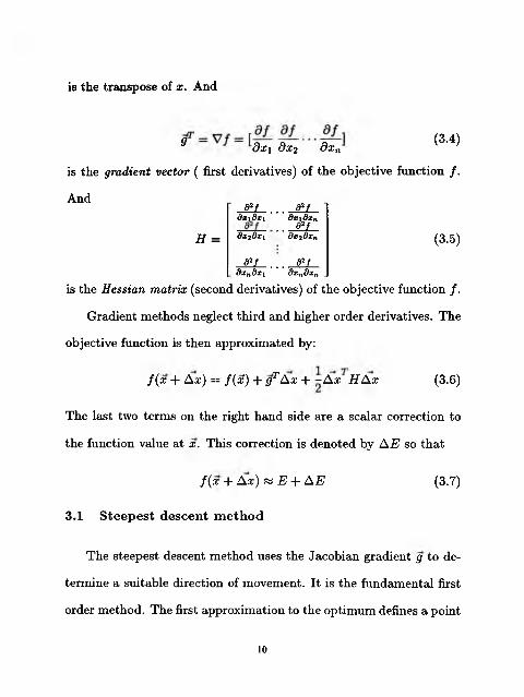
is the transpose of x. And

^ dx\ 9x2 dxn (3.4)

is the gradient vector ( first derivatives) of the objective function / .

And

H =

*7 . . . . . 02/dxjdxi dx\dxn

. . * /dxidxi 8x2dxn

a2/ a2/dxndx1 dxndxn

(3.5)

is the Hessian matrix (second derivatives) of the objective function / .

Gradient methods neglect third and higher order derivatives. The

objective function is then approximated by:

f ( x + Ax) as /(a?) + g1̂ A x + -Aa; H A x (3.6)

The last two terms on the right hand side are a scalar correction to

the function value at x. This correction is denoted by A E so that

f ( x -|- Ax) « E + A E

3.1 S teepest descent m ethod

(3.7)

The steepest descent method uses the Jacobian gradient g to de

termine a suitable direction of movement. It is the fundamental first

order method. The first approximation to the optimum defines a point

10

at which the function is evaluated to yield E and a suitable change

AE is found by evaluation of the Jacobian g. The effect on E of a

small change A x in x is given to the first order approximation by

A E = f A x (3.8)

This equation can be thought of as involving a dot product of two

vectors gT and Ax. This product is equal to:

gT A x = ||p||||Aa:|| cos 6 (3.9)

for fixed magnitudes ||p|| and ||Aa;||, A E depends on cos0, taking a

maximum positive value if 0 = 0 and a maximum negative value if

0 = 7r. The maximum reduction in E therefore occurs if 0 = 7r, from

which it follows that the minimizing change A x in x should be in the

direction of the negative gradient —g.

3.2 Steepest descent algorithm

The algorithm for implementing the steepest descent method is

the following:

1. Set A: = 0, and e as a small error value.

2. Input data Xk .

l l

3. Evaluate Ek = f ( x *) .

If ||f?* - £7*-i|| < € , output xmin = and Emin = Ek. Stop the

process .

4. Evaluate the gradient gi at point Xk-

5. Generate a new point x*+i = x*k — ctkQki w^ere ak is a constant .

6. Set k = k + 1. Goto 2.

The rate of change of the objective function at each iteration along

the direction of the negative gradient is determined by a* which could

be chosen to be a constant between 0 and 1 at all the iterations. This

method could be improved by choosing at each iteration the optimal

value of a*. This is done by the following equation:

df ( Xk ~ = 0 (3.10)da kv

which will give what is called the optimal steepest descent method. An

example of an objective function and its projection are in figures 3.1

and 3.2. The progress of the Gradient Descent algorithm is shown in

figure 3.3.

12

Figure 3.1: Example of an objective function.

Figure 3.2: Projection of the objective function.

Figure 3.3: Proceedings of the Gradient Descent method.

14

C h ap ter 4

D ecision Function For Hard C lustering - K ohonen N etw ork

The most common decision function is the Euclidean distance

defined as :

||x — itT|| = yj(x — wY(x — w) (4.1)

This rule of similarity states that the smaller the distance, the closer

are the patterns. The objective function is defined as:

E(w) = ||if — ty||2 (4.2)

The problem is reduced to:

minimize E(w) (4-3)

This objective function could be minimized by calculating the gradient

of E:

^ = - 2 ( * - * ) (4.4)

15

dEw{k) = w(k - 1) - ak~Q~jj (4.5)

which is equal to:

w(k) = w(k - 1 ) 4 - 2ak(x — w) (4.6)

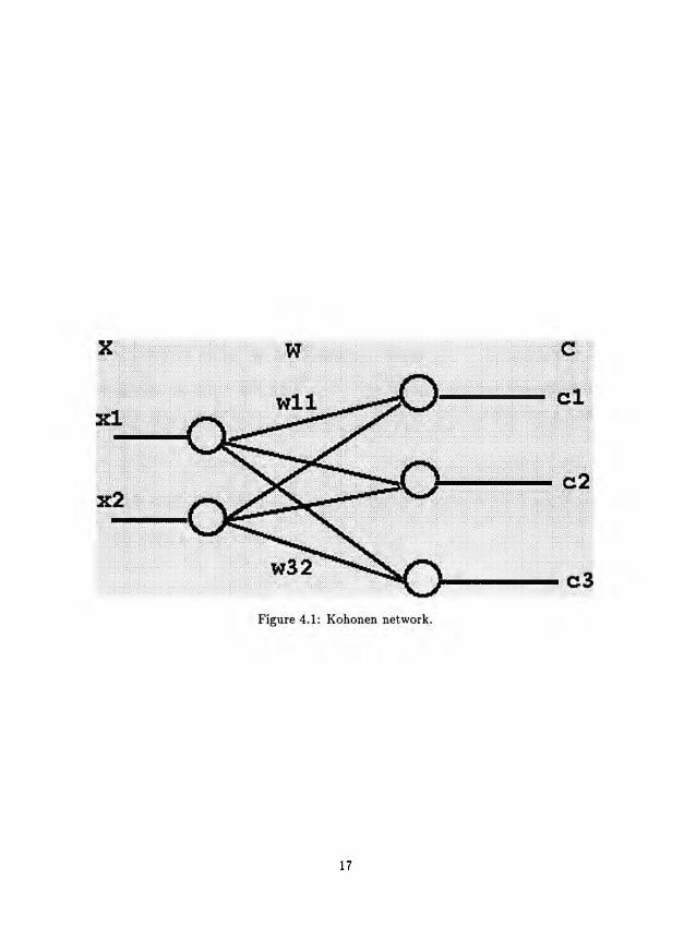
4.1 Kohonen Network

Kohonen’s network classifies input vectors into one of the specified

number of c categories according to the clusters detected in the train

ing set. The training is performed in an unsupervised mode and the

network undergoes the self-organization process. During the training,

dissimilar vectors are rejected, and only one ,the most similar, is ac

cepted for weight adaptation. In figure 4.1, the network consists of 2

inputs and 3 outputs. In general, the network consists of:

• The number of inputs which represent the dimension of the input

vector x. In our example, x is 2 dimensional vector [#1 #2].

• The number of outputs which represent the number of clusters.

In our example, 3 clusters are needed.

• And the weight vector w which will be updated at every iteration.

And then changing w by:

16

17

The updating of the weight vector is proceeded by using the Winner-

Takes-All method.

4.2 W inner-Takes-All

This learning is based on the premise that one of the neurons in

the output layer of figure 4.1 has the maximum response due to input

x. This maximum response is determined by the decision function

defined earlier (such as the Euclidian distance). This neuron is de

clared the winner. In other term, the winner is the output of the

network which has minimum distance to the input x. The learning is

proceeded as follows:

• Calculate the distances between the different weight vectors and

the input data vecor:

• The winning neuron will determine which cluster the input data

is in.

• Once the winning neuron is determined,all the weights which are

connected to that neuron will be updated using the following

formula:

D ,2\ t=l

(4.7)

w(k — 1) = w(k) + ak(x — w(k)) (4.8)

18

D ecision Function For Fuzzy C lustering - Fuzzy C -M eans A lgorithm

Kohonen network assumes that an object can belong to one and

only one class. In practice, the separation of clusters is a fuzzy notion

and hence the concept of fuzzy subsets offers special advantages over

conventional clustering by allowing algorithms to assign each object

a partial or distributed membership to each of the c clusters.

5.1 Hard vs.Fuzzy partitions

The following example designed by Bezdek illustrates the differ

ence between hard and fuzzy partitions best:

A typical 2 partitions of S = {Peach,Plum,Nectarine} can be given

as follows :

C h ap ter 5

19

Hard zl z2 z3Peach 1 0 0Plum 0 1 1

Table 5.1: Hard partitions.

where z 1 =peach,z2 =plum,and z3 =nectarine.

The table shows that for the nectarine, the hard clustering assigns full

membership to one of the two crisp subsets partitioning this data. In

this case, the nectarine is being considered as a plum ( membership

of 1). Fuzzy clustering enables algorithms to avoid such mistakes.

In the following table, the final column allocates most (0.6) of the

membership to the plum class. But also assigns a lesser membership

(0.4) to the peach class.

Fuzzy zl z2 z3Peach .9 .2 .4Plum .1 .8 .6

Table 5.2: Fuzzy partitions.

Columns such as the the one for the nectarine serve a useful pur

pose. Lack of strong membership in a single class is a signal “ to take

a second look. “ Hard partitions of data cannot suggest this.

In the following figure, 3 clusters were assumed. The membership

grade /i

• can only have 3 values el,e2,or e3 for hard clustering.

20

can span the surface E for fuzzy clustering .

Figure 5.1: Membership grades for 3 clusters.

21

5.2 Fuzzy c-means partitions

The objective function,which measures the desirability of cluster

ing candidates, is defined as:

V ) = ± ± {(& & ))"(* & ))* } (5.1)*=1 i=l

where

di($t)2 = ||f/t - (5.2)

the distance from the input data Xk to V{.

V( is the center of cluster i.

fii(xk) is the membership value of Xk in the cluster i.

m is a weighting exponent, m > 1.

c is the number of clusters.

n is the number of data.

The problem is :

Minimize Jm(/7, v). (5.3)

5.2.1 M inim ization of

The minimization of v) is done by :

^ # ^ = 0 (5.4)OfJ,

and

^ # ^ = 0 (5.5)ov

22

This will give:

i =1 dj(xk)

(5.6)

andJf _ St=! pA?h)m2k' E!=1 « ( * ) “

(5.7)

5.2.2 Fuzzy c-means algorithm

The algorithm for implementing this method is as follows :

1. Fix c, 2 < c < n.

Fix m, 1 < m < oo.

Fix e as a small positive error number.

2. Initialize the cluster centers Vi(t) .

3. Input data X = {#1 , • • • ,xn}.

4. Update V{(t + 1) then calculate //*(#*).

5. calculate the error e = ||ui(t + 1) — *T,-(t)||

if e < e output /x,- and u,- , stop.

else goto step 3.

23

G radient B ased Fuzzy C -M eans A lgorithm

One attempt to improve the FCM algorithm in this thesis is made

by minimizing the objective function using one datum at a time in

stead of the whole data at once.

6.1 Derivation of the algorithm

Given one datum X{ and c clusters with centers at Vj (j = 1,2, • • •, c),

the objective function to be minimized is :

Ji = - *.11 + t4i\Wi - **ll + • • • + /4 ||vc - X<|| (6.1)

with the constraint:

/^li + V>2i + •• + fj>ci = 1 (6 -2 )

The basic procedure of the gradient descent method is that starting

from an initial center vector u, the gradient VJ* of the current ob

jective function is computed [10]. The next value of v is obtained by

C h ap ter 6

24

moving in the direction of the negative gradient along the multidi

mensional error surface such that:

«*+i = «r* - (6.3)

where :

Equivalently,

'dvk

= 2 nli(vk- Si) (6.4)

V*+1 = V k - r ) /4 i(vk - Xi) (6.5)

where rj is a small learning constant.

For the membership grades, we set :

P = 0 (6.6)Of!

and obtain :

flki = ------------ ■ (6‘7)'pc ( dj(xk) \^j= 1 V

6.2 Com parison betw een FCM and G BFCM

FCM and GBFCM both have an objective function which tries to

minimize the distance between each center and the data with a mem

bership grade reflecting the degree of their similarities with respect to

other centers. On the other hand, they differ in the way they try to

minimize it:

25

• In the FCM algorithm, all the data are present in the objective

function, and the gradients are set to zero in order to obtain the

equations necessary for minimization[2-5] .

• In the GBFCM, only one datum is present at a time. And only

the gradients of the objective function with respect to the mem

bership grades are set to zero. The gradients with respect to

the centers are not set to zero, their negative values are used to

minimize the objective function.

6.3 G BFCM algorithm

The algorithm for implementing this method is as follows :

Procedure main()Read c,€,m

W hile (error > e ) e <— 0

W hile (input file is not empty ) Read one datum X {

Vk+i * - v k - rwli(vk ~ Xi)

e «— e + V i ( k + 1) — V i ( k )

end while error <— e

end while O utput f i { and v,-.

end main()

26

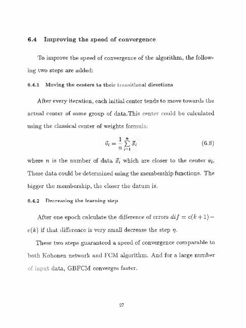
6.4 Im proving th e speed o f convergence

To improve the speed of convergence of the algorithm, the follow

ing two steps are added:

6.4.1 M oving the centers to their transitional directions

After every iteration, each initial center tends to move towards the

actual center of some group of data.This center could be calculated

using the classical center of weights formula:

tTi = - E x i (6.8)n i=i

where n is the number of data X{ which are closer to the center

These data could be determined using the membership functions. The

bigger the membership, the closer the datum is.

6.4.2 Decreasing the learning step

After one epoch calculate the difference of errors d if = e(k +1) —

e(k) if that difference is very small decrease the step tj.

These two steps guaranteed a speed of convergence comparable to

both Kohonen network and FCM algorithm. And for a large number

of input data, GBFCM converges faster.

27

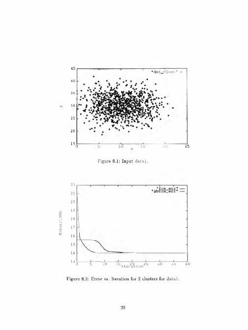
6.5 Convergence o f GBFCM vs. FCM

To show the convergence of GBFCM vs. FCM, input data were

created using the gaussian distribution. And the behavior of the error

with respect to each iteration for both algorithm were recorded. The

following graphs were obtained:

28

Erro

r/10

0045

40

35

>1 30

25

20

150 5 10 15 20 25x

Figure 6.1: Input data l.

22

21 20

19 18 17 16 15 14

13 0 5 10 15. _ 20_. 25 30 35 40iteration

Figure 6.2: Error vs. iteration for 2 clusters for d ata l.

■datclust" ♦

♦♦

29

Error/1000

Error/1000

Figure 6.3: Error vs. iteration for 3 dusters for datal.

Figure 6.4: Error vs. iteration for 4 dusters for datal.

30

Error/100000

90 80 70 60 50 40 30 20

10

°0 ’ 5 ’ 10 15 20 25x

Figure 6.5: Input data2

"dat_clust" ♦

Figure 6.6: Error vs. iteration for 2 clusters for data2.

31

Error/100000

Erro

r/10

0000



32

Figure 6.9: Input data3


Erro

r/10

000



34

A pplication O f G B FC M To Im age Segm entation

Image segmentation is defined as subdivision of an image into its

constituent parts or objects. This is achieved generally based on one of

two basic properties of gray level values: discontinuity and similarity.

The detection of discontinuities approach, is to partition an image

based on abrupt changes in gray level. Therefore, detection of isolated

points, lines and detection of edges fall into this category. On the

other hand detection of similarities approach is based on thresholding,

region growing, and region splitting and merging.

7.1 D etection of edges

By definition, an edge is the boundary between two regions with

relatively distinct gray-level properties. For edge detection to work

as a tool for image segmentation, the regions under investigation are

C h ap ter 7

35

sufficiently homogeneous so that the transition between two regions

can be determined on the basis of gray level discontinuities alone. The

basic tool used for edge detection is taking the derivative or gradient

of the image. The gradient of an image f(x,y) at location (x,y) is the

vector given by,

V / = (7.1). dy .

It is important to mention a popular and important operator known

as the Laplacian of the Gaussian. The Gaussian is defined as:

G(a!)y) = 2^ ea:p(" ^ " ) (7'2)

The Laplacain of the Gaussian is defined as:

CM)

1 x2 + y2 — 2a2 f x2 + y2

Which will give:

^ ~ ™

Applying the Laplacian of the Guassian to an image f ( x , y) is given

by:

f ( x ,y ) * V 2G(x,y) (7.5)

where * is the convolution operator.

This operator will be transformed into regular multiplication in the

36

frequency domain.

F (f(x , y) * V 2G(x, y)) = F (f(x , y)F(V2G(x, y)) (7.6)

where F is the Fourier transform.

The final output is the inverse of the Fourier transform obtained:

F -\F ( f(x ,y )F (V 2G(x,y))) (7.7)

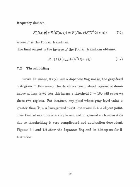
7.2 Thresholding

Given an image, f(x,y), like a Japanese flag image, the gray-level

histogram of this image clearly shows two distinct regions of domi

nance in gray level. For this image a threshold T = 100 will separate

these two regions. For instance, any pixel whose gray level value is

greater than T, is a background point, otherwise it is a object point.

This kind of example is a simple one and in general such separation

due to thresholding is very complicated and application dependent.

Figures 7.1 and 7.2 show the Japanese flag and its histogram for il

lustration.

37

Iv Iv a . / a v I . X v w v / w .'•>% ■''

Figure 7.1: Image of the Japanese flag .

grey le v e l g

Figure 7.2: Histogram of the Japanese flag.

38

7.3 R egion Splitting and M erging

The technique of region splitting and merging can be summarized

as follows:

1. Split the image into four equal parts with no intersection.

2. If all the pixels in a region R{ possess approximately the same

property then splitting of that region is complete and it is left

alone. ( The property of the pixels depends on the application,

and on the type of segmentation involved).

3. If the pixels in a region i?, , do not possess approximately the same

property, it is split again into four other disjoint regions. After

this, the regions with similar properties are merged together to

form one region.

7.4 U nsupervised im age segm entation

The following steps are taken in applying the unsupervised image

segmentation:

1. A sliding window of size Ml x N1 is selected and the window is

moved through the image at displacements M2 horizontally and

N2 vertically.

39

2. At each window position, certain window parameters are esti

mated from the data and stored as a vector.

3. Then the number of clusters in the set of parameter vectors are

identified.

4. Finally, the image is segmented.

7.4.1 Im plem entation

For the implementation part, a 256 x 256 image was used, and a 16

x 16 sliding window was selected. In addition, the model parameters

for each window were the mean and standard deviation. The formulas

used to calculate the mean and standard deviation of all the pixels in

a particular window are shown respectively below.

m = j j ' £ x i(7.8)

= (*<-">)* (7-9)

where N is the total number of pixels in the sliding window, and X{

is the gray level value of pixel position i in the window. The data

available were the mean and standard deviation of each window. The

unsupervised learning is used to to cluster the data. The number of

clusters obtained depends on the level of segmentation desired.

40

Furthermore, after the centers of the desired clusters were obtained,

segmentation of the image took place as follows:

1. Each pixel was compared to all the centers obtained using the

gaussian density function :

Gi(x) = 2ira%eX 2of (7-10)

2. Each pixel was then assigned the value of the center of a particular

cluster based on the following formula:

x = rrik (7-11)

where

k = max(G,*(a:)) 0 < i < c (7-12)

c is the number of clusters.

7.4.2 Results

Depending on the level of segmentation ( number of clusters )

chosen, the following images are obtained for 2,3,and 4 clusters.

41

Figure 7.3: Imagel of Lenna .

Figure 7.4: 2-level segmentation of imagel.

42

Figure 7.5: 3-level segmentation of im agel.

Figure 7.6: 4-level segmentation of imagel.

43

Figure 7.7: Image2 of a walkway.

Figure 7.8: 2-level segmentation of image2.

44



45

Figure 7.11: Image3 of a scene.



l i i l l■ s i

m m


7.5 Stopping G BFC M and FCM at different iterations

A 4-level segmentation of the Lenna image has been implemented.

FCM and GBFCM were compared by stopping the algorithms at

2,4,6,and 8 iterations .

Figure 7.15: Mean vs. standard deviation for the Lenna image.

Figure 7.16: Error vs. iteration for 4 clusters.

48

Figure 7.17: FCM 4 clusters - 2 iterations.

Figure 7.18: GBFCM 4 clusters - 2 iterations.

49



50



51



52

7.6 D iscussion

Stopping the algorithms at different iterations,as shown in the above

figures, is a strong tool which can be used to show the progress of

an algorithm. Starting at 2 iterations,FCM algorithm couldnot yet

distinguish between 2 regions (clusters) of the input data (figure 7.15).

Only one region could be seen (figure 7.17). GBFCM algorithm,on

the other hand, clustered the data into at least 2 regions (figure 7.18).

Going to 4 iterations figure 4 shows that the FCM algorithm started

to distinguish between 2 levels ( at least 3 levels for the GBFCM

algorithm ). Increasing the number of iterations has the effect of

clustering the data into the 4 regions desired (4-level segmentation)

as shown in figures 7.23 and 7.24.

53

A pplication O f G B FC M To R egression A nalysis

Regression analysis is a statistical technique for investigating and

modeling the relationship between variables. It is used to develop

equations which summarize or describe the behavior of a set of data.

To develop these equations, the following 2 steps should be taken:

1. Building a regression model.

2. Estimating the parameters of the model.

The data are used to estimate the unknown parameters of the system.

8.1 Least squares estim ation of the parameters

A regression model could be given by the following relationship:

y = f(x,/3) + e (8.1)

C h ap ter 8

54

f3 is a vector of parameters to be determined.

e random vector with mean vector 0 and covariance matrix (

Regression analysis is defined as the search for the best function /

which will fit a set of observed data. S = {(a?i, yi), • • •, (xn, yn)} The

method of least squares is used to estimate the vector /3. This vector

will be estimated so that the sum of the squares of the differences

between the observations y#* and the response of the model y is a

minimum.Thus the least squares criterion is

m = £ ( y i - f ( x i , p ) - e i)2 (8.2)i= 1

The least squares estimators of (3 must satisfy:

I - ° <8-3>

which will give the value of the vector f3.

8.2 U nsupervised regression analysis

Unsupervised regression analysis is a generalization of the regres

sion discussed earlier in the following 2 ways:

1. More than a single model are assumed.

2. And at the same time 5 = {(®i, 2/i), • • • » 2/n)} is not labeled.

55

Thus, instead of assuming that a single model can can account for all

n pairs in S, the data can be drawn from c models.

y = fi(x, Pi) + €,• 1 < (8.4)

and for a given (#*, y*) it is not known which model can be applied.

8.3 Unsupervised learning - O bjective function

Because the data set S is unlabeled, the problem is to assign

to each pair of data in 5 labels (memberships) which will identify its

degrees of belongings to each model (group) considered. This is called

unsupervised learning where the memberships /z are interpreted as the

importance or weight attached to the extent to which the model value

fi(x, Pi) matches y*. Crisp memberships would place all of the weight

in the approximation of y* by fi(x,/3{) on one class for each k. But

fuzzy partitions can represent situations where a data point fits all

the models to varying degrees.

8.3.1 Objective function

For one pair of data (x, y), the error function can be defined as:

Ei(pi) = \ \ y - f i ( x ,p i ) \ \ 2 (8-5)

56

which measures the error in /«(#, Pi) as an approximation to y.

Considering all the c models, the objective function is:

= (8-6) 1=1

8.3.2 Estim ating the parameters of the system

The minimization of J(fi,P) is done by :

0 (8.7)0/1

and

A+i = f t - (8.8)

Using these 2 formulas, the parameters P and fi could be calculated

(tj is a small learning constant which decreases as learning proceeds).

57

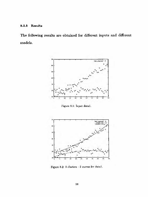
8.3 .3 R esu lts

The following results axe obtained for different inputs and different

models.

Figure 8.1: Input d ata l.

Figure 8.2: 2 clusters - 2 curves for d ata l.

58

* 0 0 0 I I | I ■ I I 1~'d«t ngnit* * • ♦

2000 *♦ ♦

• •♦

♦ ♦ #• • • .

-2000 h

♦♦.4000 I .1_______ I_______ I_______ I I - I I I

0 5 10 15 20 25 30 35 40 45 50

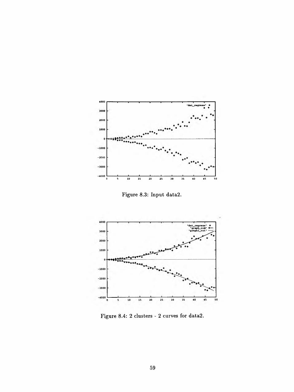
Figure 8.3: Input data2.

Figure 8.4: 2 clusters - 2 curves for data2.

59

Figure 8.5: Input data3.

Figure 8.6: 3 clusters - 3 curves for data3.

60

C h ap ter 9

A pplication O f G B FC M To R eduction o f features o f th e Fourier transform o f th e EM G signal

The source of the bioelectric signal is the single neural or muscular

cell. The accumulated effects of all active cells in the vicinity produce

an electric field which creates important electric signals used for the

diagnosis of neural and muscular systems. Electromyographic (EMG)

is the recording of the electric potential generated by the muscle.

EMG signals are nonperiodic and possess all the characteristics of a

random signal [16]. They can be anlysed using Fourier analysis which

extracts features that characterize the important aspects of the signal.

61

9.1 Signal classification and recognition

The recognition of the signal is done by means of a classification

process. The machine has a priori knowledge on the types (classes)

of signals under consideration. An unknown signal is then classified

into one of the known classes. The mechanism could be represented

by:

1. The input to the recognition machine is a set of N measurements

(samples of the signal).

2. A set of features is then extracted (Fourier transform).

3. And a classifier operates on the feature vector to perform the

classification.

..... \ \ Feature \/ Measurement ? extraction ? classifier

sampling Fourier transform decision functionFigure 9.1: Signal classification.

9.2 N eural networks as a classifier

In this method :

• A neural network (NN)is used to classify the data.

62

• The number of classes desired is 3 :min,mid, and max types.

These represent low,medium,and high level muscle activity respec

tively. The first set of data was collected with the arm being in a

resting position with very little firing of muscles. The second set

was collected with arm muscles being semi-tense. The third set was

collected with arm muscles being in a tense position. For every set

Fourier transform is applied to the data collected .

9.3 U nsupervised learning

A different approach based on the use of the unsupervised learning

which is capable of reducing the number of features obtained by the

Fourier analysis. Then these reduced features will be used to train a

NN with less number of neurons than the one used before.

63

EMG

JLm il

I T "H ill i $ i !

Figure 9.2: Neural network as a classifier.

m o * ■ ■■■ X63

unsupervisedfeaturesreduction

I I

Figure 9.3: Reduction of features using GBFCM algorithm.

64

The following figures represent 2 patterns of the resting position:

0 . 0 8

0 . 0 7

0 . 0 6

0.0S

I °-M0 . 0 3

0 . 0 2

0.01

° 0 10 20 30 40 50 60 70frequency

Figure 9.4: Pattern 1 of the resting position.

0 . 0 8

0 . 0 7

0 . 0 6

0 . 0 5

| 0 . 0 4

0 . 0 3

0 . 0 2

0.01

0

Figure 9.5: Pattern 2 of the resting position.

65

The following figures represent 2 patterns of the arm in the mid

position:

Figure 9.6: Pattern 1 of the mid position.

Figure 9.7: Pattern 2 of the mid position.

66

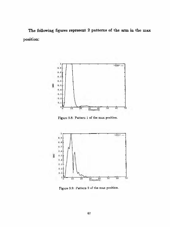
The following figures represent 2 patterns of the arm in the max

position:

Figure 9.8: Pattern 1 of the max position.

Figure 9.9: Pattern 2 of the max position.

67

Applying unsupervised learning to these patterns will give:

Figure 9.10: 6-point patterns for the min position.

Figure 9.11: 6-point patterns for the mid position.

68

Membership

Function

F(x)

° 0 0 . 5 1 1 . 5 2 2 . 5 3 3 . 5 4 4 . 5X

Figure 9.12: 6-point patterns for the max position

69

9.4 R esults

The following table is obtained after testing the network with un

trained data:

Pattern EMG (rest) EMG (betweenl) EMG (mid)EMG(rest) 95.92% 4.08% 0%

Table 9.1: Untrained rest test data results.

Pattern EMG (mid) EMG (between2) EMG (max)EMG (mid) 91.81% 8.19% 0%

Table 9.2: Untrained mid test data results.

Pattern EMG (between2) EMG(max)EMG (max) 7.7% 92.3%

Table 9.3: Untrained max test data results.

70

Chapter 10

C onclusions

A Gradient-Based FCM (GBFCM) algorithm is presented. This

algorithm combines the characteristics of Kohonen network (Requir

ing one datum at a time in a gradient fashion) and Fuzzy c-means

algorithm (fuzzy membership in {0, • • •, 1}). Both FCM and GBFCM

were applied to the same problem (4-level segmentation). The ex

periments performed in this thesis such as clustering of random data,

image segmentation, regression analysis, and reduction of features of

the EMG signal show that GBFCM converges faster giving competi

tive results when compared to FCM.

10.1 Future Work

GBFCM algorithm proceeds using the gradient descent method

which could be improved in terms of speed of convergence and com

plexity of calculations. This could be done using the :

71

1. conjugate gradient method which is much faster than the gradient

descent method.

2. genetic algorithm which doesn’t require the calculation of any

derivative.

Both of these methods could be used for future improvements.

72

Bibliography

[1] J.M.Zurada, Artificial neural systems, West 1992

[2] T. Kohonen,“ Learning Vector Quantization, “ Helsinki University

of Technology, Laboratory of Computer and Information Science,

Report TKK-F-A-601, 1986

[3] J.C.Dunn, UA fuzzy relative of the ISODATA process and its

use in detecting compact well separated clusters, “ J. Cybem.,

1973,(3) :32-75.

[4] J.C.Bezdek, “ A convergence theorem fo the fuzzy ISODATA

clustering algorithms,“IEEE trans. pattern Anal. Mach. int.,

1980,(2):l-8. 1975,(24):835-838.

[5] Windham M.P., “Cluster Validity for the Fuzzy c-means

clustering algorithm, “IEEE trans. pattern Anal. Mach. int.,

1982, (4) *.357-363.

73

[6] I.Gath,A.B.Geva, “Unsupervised optimal fuzzy clustering,44

IEEE trans. pattern Anal. Mach. int., 1989,(11):773-781.

[7] Rafael C. Gonzalez and Richard E. Woods,Digital Image Process-

ing, New York: Addison-Wesley, 1992.

[8] Young Won Lim and Sang Uk Lee,” On the color image segmenta

tion algorithm based on the thresholding and the Fuzzy c-means

techniques/4 Pattern Recognition, vol.23,no.9,1990.

[9] J.C.Bezdek, Pattern recognition with fuzzy objective function al

gorithms, New York: Plenum,1981.

[10] B.S .Gottfried,J.weisman, Introduction to optimization theory ,

Prentice Hall 1973

[11] J.C.Bezdek,J.C.Dunn/4 Optimal fuzzy partition:A heuristic for

estimating the parameters in a mixture of normal distributions/4

IEEE Trans. Comput., 1975,(24):835-838.

[12] Xuanli 1.x.,BEN G., 44 A validity measure for fuzzy clustering/4

IEEE trans. pattern Anal. Mach. int., 1991,(13):841-847.

[13] J. Hertz et al., Introduction to the Theory of Neural Computation,

Reading, MA: Addison-Wesley, 1990

74

[14] G.J.Klir,T.A.Folger, Fuzzy sets, uncertainty, and information ,

Prentice Hall 1988

[15] Dong C. Park and Issam Dagher, “Gradient Based Fuzzy c-means

( GBFCM ) agorithm,“ Proc. of IEEE World Congress on Com

putational Intelligence ’94,Orlando,June26-July2, 1994.

[16] Adrian Del Boca and Dong C. Park, “ Myoelectric Signal

Recognition using Artificial Neural Networks in Real Time

, “Proc. of IEEE World Congress on Computational Intelligence

’94, Orlando, June26-July2, 1994.

[17] V.Tiel, Convex Analysis, Wiley 1984

[18] J. Zhang and J. W. Modestino,“A Model Fitting Approach To

Cluster Validation, “ IEEE Transactions On Pattern Analysis

And Machine Intelligence, Vol. 12, No. 10, October 1990.

[19] C. Bouman and B. Liu.,“Multiple Resolution Segmentation of

Textured Images/4 IEEE Transactions On Pattern Analysis And

Machine Intelligence, PAMI-13, 1991, 99-113.

[20] Haluk Derin, and Howard Eliot,“Modelling and Segmentation

of Noisy and Textured Images Using Gibbs Random Fields/4

75

IEEE Transactions On Pattern Analysis And Machine Intelli

gence, Vol.PAMI-9, No. 1, January 1987.

[21] Hong Hai Nguyen and Paul Cohen, “Gibbs Random Fields, Fuzzy

Clustering, and the Unsupervised Segmentation Of Textured Im

ages, “ Graphical Models And Image Processing, Vol. 55, No.

1,January, pp. 1-19, 1993.

[22] Chee Sun Won And Haluk Derin. “Unsupervised Segmenta

tion of Noisy and Textured Images Using Markov Random

Fields, “ Graphical Models And Image Processing, Vol. 54, No. 4,

July, pp. 308-328,1992.

[23] R. J.Hathaway and J.C.Bezdek, “Switching Regression models and

Fuzzy Clustering, UIEEE Transactions on Fuzzy Systems, Vol.

l,No. 3,August 1993.

[24] R.D.De Veaux, “Mixtures of linear regression, “ Computational

Statistics and Data Analysis, Vol. 8,pp 227-245, 1989.

[25] M.Aitkin and G.T.Wilson,“Mixture models,outliers,and the EM

algorithm,u Technometrics, Vol. 22,No. 3, 1980.

[26] R.E.Quandt,“A new approach to estimating switching regres

sions,14 J. Amer. Stat. Ass., Vol. 67,pp. 306-310, 1972.

76

[27] R.E.Quandt and J .B.Ramsey,“Estimating mixtures of normal

distributions and switching regressions/* J. Amer. Stat. Ass.,

Vol. 73,pp. 730-752, 1987.

[28] R.J.Hathaway and J.C.Bezdek, “Numerical convergence and in

terpretation of the fuzzy c- shells clustering algorithm/* IEEE

Trans. Neural Networks, Vol, 3,pp. 787-793,Sept. 1992.

[29] Sanford Weibeig, Applied Linear Regression, New York: John Wi

ley , 1980.

[30] Douglas C. Montgomery And Elizabeth A.Peck,Introduction to

Linear Regression Analysis, New York: John Wiley , 1982.

77

Documents

Gradient based fuzzy c-means algorithm - FIU Digital Commons