GPU-based Parallel Computation Support for Stan · Stan has three distinct components: a probabilistic programming language, the Stan Math librarythatsupportsauto-diﬀerentiation,andalgorithmsforinference

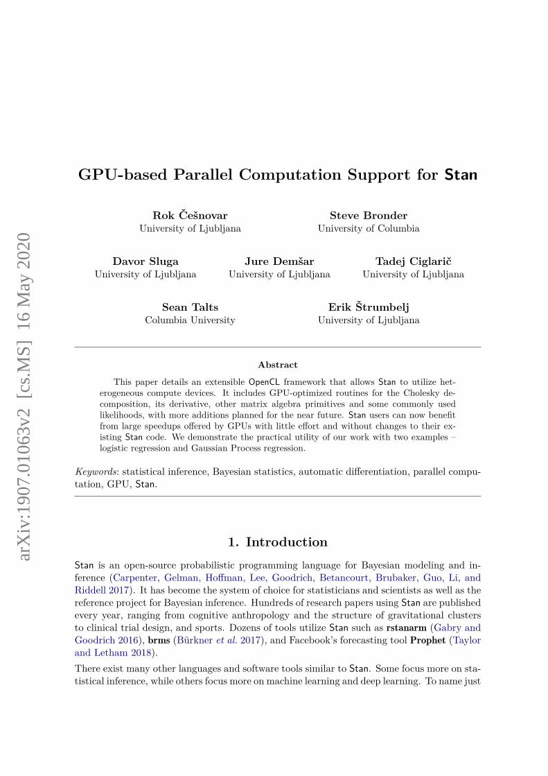
GPU-based Parallel Computation Support for Stan

Rok ČešnovarUniversity of Ljubljana

Steve BronderUniversity of Columbia

Davor SlugaUniversity of Ljubljana

Jure DemšarUniversity of Ljubljana

Tadej CiglaričUniversity of Ljubljana

Sean TaltsColumbia University

Erik ŠtrumbeljUniversity of Ljubljana

Abstract

This paper details an extensible OpenCL framework that allows Stan to utilize het-erogeneous compute devices. It includes GPU-optimized routines for the Cholesky de-composition, its derivative, other matrix algebra primitives and some commonly usedlikelihoods, with more additions planned for the near future. Stan users can now benefitfrom large speedups offered by GPUs with little effort and without changes to their ex-isting Stan code. We demonstrate the practical utility of our work with two examples –logistic regression and Gaussian Process regression.

Keywords: statistical inference, Bayesian statistics, automatic differentiation, parallel compu-tation, GPU, Stan.

1. IntroductionStan is an open-source probabilistic programming language for Bayesian modeling and in-ference (Carpenter, Gelman, Hoffman, Lee, Goodrich, Betancourt, Brubaker, Guo, Li, andRiddell 2017). It has become the system of choice for statisticians and scientists as well as thereference project for Bayesian inference. Hundreds of research papers using Stan are publishedevery year, ranging from cognitive anthropology and the structure of gravitational clustersto clinical trial design, and sports. Dozens of tools utilize Stan such as rstanarm (Gabry andGoodrich 2016), brms (Bürkner et al. 2017), and Facebook’s forecasting tool Prophet (Taylorand Letham 2018).There exist many other languages and software tools similar to Stan. Some focus more on sta-tistical inference, while others focus more on machine learning and deep learning. To name just

arX

iv:1

907.

0106

3v2

[cs

.MS]

16

May

202

0

2 GPU-based Parallel Computation Support for Stan

a few of the most popular: Edward/Edward2 (TensorFlow) (Tran, Hoffman, Saurous, Brevdo,Murphy, and Blei 2017) and PyMC3 (Salvatier, Wiecki, and Fonnesbeck 2016) (Theano)(Bergstra, Breuleux, Bastien, Lamblin, Pascanu, Desjardins, Turian, Warde-Farley, and Ben-gio 2010), Pyro (Bingham, Chen, Jankowiak, Obermeyer, Pradhan, Karaletsos, Singh, Szerlip,Horsfall, and Goodman 2019) (PyTorch) (Paszke, Gross, Chintala, Chanan, Yang, DeVito,Lin, Desmaison, Antiga, and Lerer 2017), and MxNet (Zheng, Chen, Li, Li, Lin, Wang, Wang,Xiao, Xu, Zhang, and Zhang 2015).Stan has three distinct components: a probabilistic programming language, the Stan Mathlibrary that supports automatic differentiation, and algorithms for inference. The main ad-vantages of Stan are a rich math library and state-of-the-art inference with a variant of Hamil-tonian Monte Carlo – the NUTS (No-U-turn) sampler (Hoffman and Gelman 2014) with someadditional modifications (Betancourt 2017a; Stan Development Team 2020) – which makesStan suitable for robust fully-Bayesian inference. Moreover, the Stan probabilistic program-ming language is easier to understand than systems embedded in other languages (Baudart,Hirzel, and Mandel 2018).Stan has only recently started building out low-level parallelism. While Stan supports thread-ing and MPI to execute disjoint sets in the automatic differentiation expression tree, it did nothave support for specialized hardware such as GPUs. An ideal case for GPU based optimiza-tion are models based on Gaussian Processes (GP). The computation in GP-based models is,even for moderate input sizes, dominated by computing the inverse of the covariance matrix.The O(n3) time of this operation also dominates the quadratic costs associated with trans-ferring matrices to and from a GPU. In turn, computing the Cholesky decomposition of thepositive definite matrix dominates the computation time of the matrix inverse. Because thesecosts can be broken up and executed in parallel they make the Cholesky decomposition anideal target for GPU-based computation.This paper describes a framework for GPU support in Stan and GPU implementations of theCholesky decomposition, its derivative, other matrix algebra primitives, and GLM likelihoodswith derivatives in the Stan Math library. Unlike most similar libraries, our framework relieson OpenCL 1.2 (Stone, Gohara, and Shi 2010), so it supports a variety of devices. Thisincludes GPUs of different vendors, multi-core CPUs, and other accelerators.The integration with Stan is seamless and user friendly - setting a flag moves the computationof supported routines to the GPU, with no need to change Stan code. The API providesexperts with a simple way of implementing their GPU kernels, using existing GPU kernels asbuilding blocks. We demonstrate the practical utility of our work – ease of use and speedups– with two examples, logistic regression and Gaussian Process regression.

2. Integrating OpenCL with StanStan’s reverse mode automatic differentiation uses the Matrix type from Eigen (Guennebaud,Jacob et al. 2010) to store data as a matrix of type double or Stan’s var type, where the varholds the value and adjoint used in automatic differentiation. Stan builds up an expressiontree used in automatic differentiation and stores all the data needed in the expression treevia its local allocator. When a node’s children in the expression graph are disjoint, Stan canutilize C++11 threading or MPI to compute the log probability evaluation in parallel. Whenan operation within a node is expensive, Stan can use the OpenCL backend to parallelize the

Journal of Statistical Software 3

operation on the node.

2.1. OpenCL baseStan’s OpenCL backend uses a single context to receive data and routines from individualnodes in the expression tree. Ensuring there is only one context and queue per device for thelife of the program makes context management simpler. The implementation of the OpenCLcontext which manages the device queue follows the singleton pattern and sits in the classopencl_context_base.Instead of calling opencl_context_base::getInstance().method(), developers can access thecontext through a friend adapter class opencl_context which provides an API for accessingthe base context. If the OpenCL implementation supports asynchronous operations, then thecontext asynchronously executes kernels. Asynchronous operations are particularly usefulin conjunction with threading as the individual threads will be able to enqueue operations,which will execute while threads do other calculations using CPU.

2.2. Matrix classThe base matrix class matrix_cl holds the device memory buffer, meta-information onthe matrix, and methods for reading and writing event stacks for asynchronous computa-tion. When a kernel receives a matrix_cl, the kernel’s event is attached to the appro-priate read or write event stack. Reading and writing to OpenCL buffers uses the genericenqueue(Write)/(Read)Buffer methods. Because Stan Math heavily relies on Eigen matri-ces, constructors and methods are available for easily passing data back and forth.Developers can pass in Eigen matrices directly to the matrix_cl constructor or use theto_matrix_cl() or from_matrix_cl() methods.

Eigen:: MatrixXd m(2, 2);m << 1, 2, 3, 4;

matrix_cl A(m);matrix_cl B(2, 2);

B = to_matrix_cl(m);Eigen:: MatrixXd C = from_matrix_cl(B);

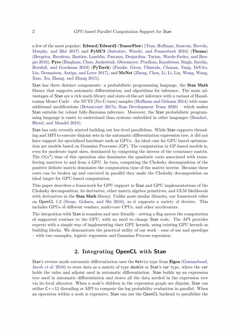
Similar constructors for the matrix_cl class are available for standard vectors std::vector<T>and arrays of doubles.We can reduce the data transfers of triangular matrices by only transferring the non-zeroparts of the matrix in a packed form. The kernel unpack deals with unpacking the packedform shown on the right-hand side on Figure 1 to a flat matrix shown on the left-hand side.For lower (upper) triangular matrices, the irrelevant upper (lower) triangular is filled withzeros. The kernel pack packs the flat matrix to packed form for the transfer back to the host’sglobal memory.

matrix_cl L = packed_copy <stan::math:: matrix_cl_view ::Lower >(L_val_cpu , M_);

When operating on GPUs, transferring data from host to device and making copies can bethe most expensive operations. To reduce the burden of data transfers, the Stan compileridentifies immutable data objects. These objects are copied to the GPU at the start andremain on the GPU until the end of inference.


Figure 1: Packing and unpacking a triangular matrix.

Note that matrix_cl supports direct allocation of a matrix of var objects (used for parametersfor the purpose of automatic differentiation) - this stores two separate matrices, one for valuesand the other for adjoints, which simplifies the API.

2.3. Kernel construction

The OpenCL specification demands that strings are used to represent OpenCL kernels. How-ever, having a large number of files comprised of strings is unwieldy and difficult to maintain.Stan wraps its kernels inside of a STRINGIFY macro, which gives developers access to the stan-dard set of developer tools such as code highlighting, linting, Doxygen (Van Heesch 2008),and auto-formatting. This style makes the kernel code easier to maintain compared to havingfiles full of strings. An example of how a developer brings a new kernel into Stan:

// Items in between \ cond and \ endcond are ignored by doxygen .// \ condconst char * example_kernel_code = STRINGIFY (// \ endcond/*** Example of adding new kernel in Stan** @param [ out] A An example output matrix .* @param [in] B An example input matrix .* @param val Some other input value*/__kernel void example ( double *A, double *B, int * val ) {// kernel code ...}// \ cond);// \ endcond/*** See the docs for \ link kernels / example .hpp example () \ endlink*/const kernel_cl < out_buffer , in_buffer , int > example ("␣example␣", example_kernel_code , {"␣THREAD_BLOCK_SIZE␣", 32});

In the above, a developer uses STRINGIFY to create a const char* that holds the kernel code.That string passes into the kernel_cl struct templated by the kernel argument types andwith arguments giving the name of the kernel, the kernel code, and optional kernel macrosthey would like to have defined in the kernel.Internally, we keep track of OpenCL events via queues on each matrix_cl object that we useto conservatively prevent race conditions and provide ordering where necessary. out_bufferand in_buffer are empty structs that we pass as template arguments to configure the kernelduring construction to indicate the directionality of each input buffer. At runtime, the kernel


will check the correct event queues on its arguments for events it needs to wait for and thenattach the event representing the kernel’s completion to each buffer’s queues correctly. Thatway we ensure that an operation that, for example, writes to a buffer, is completed before weallow the OpenCL runtime to read from that buffer.The parameter pack of types in the template for kernel_cl are unpacked and passed downas the argument types for the operator() and down to the template arguments for OpenCL’smake_kernel functor. Below is a simplified version of the code used to construct and call thekernel.

template <typename ... Args >struct kernel_cl {

const kernel_functor <to_const_buffer_t <Args >&...> make_functor;

kernel_cl(const char* name , const std::vector <const char*>& sources ,const std::map <const char*, int >& options = {})

: make_functor(name , sources , options) {}

auto operator ()(cl:: NDRange global_thread_size , cl:: NDRange thread_block_size ,to_const_matrix_cl_t <Args >&... args) const {

auto f = make_functor ();

const std::vector <cl::Event > kernel_events= vec_concat(select_events <Args >(args )...);

cl:: EnqueueArgs eargs(opencl_context.queue(), kernel_events ,global_thread_size , thread_block_size );

cl::Event kern_event = f(eargs , get_kernel_args(args )...);

assign_events <Args ...>( kern_event , args ...);return kern_event;

}};

Note that the meta-programming traits to_const_buffer_t<> and to_const_matrix_cl_t<>override the in_buffer and out_buffer template types in order to propagate a cl::Bufferor matrix_cl to subsequent templates and signatures.In the above code, the kernel_cl’s constructor passes the name, kernel code, and kerneloptions to the kernel functor in the initialization list which compiles the kernel. Kernelarguments declared with in_buffer or out_buffer should be of type matrix_cl. When akernel is called, the events that are in each matrix_cl’s read or write stacks are collecteddepending on whether it was designated as an in or out buffer. The kernel will then wait toexecute until the previous events complete. The kernel’s event is assigned to each matrix_cl’sread and write event stack via assign_events() depending on whether it was defined as anin_buffer or an out_buffer.When the kernel_cl struct is constructed, it compiles the kernel and developers call thekernel with

matrix_cl foo = //...matrix_cl goo;example(cl:: NDRange (...), goo , foo , 10);

Depending on the in/out_buffer passed when constructing the kernel, events will be added


to the appropriate matrix_cl read and/or write event stack. For instance, in the above, gooin the output and will have the kernel’s event attached to it’s write_stack. While foo willhave the kernel’s event attached to its read_stack. Later kernel calls that write to foo willknow to wait for all the events in foo’s read_stack and write_stack while kernels that usegoo as input will know to wait for the event’s in goo’s write_stack.The kernel functions for addition, subtraction, and multiplication are wrapped in their stan-dard operators so users of the Stan Math library can call the operations such as:

matrix_cl A = B * C + D - E;

3. GPU-optimized routines in the Stan Math libraryIn this section we describe the three GPU-optimized matrix algebra primitives that are cur-rently implemented in Stan Math. They are currently not accessible directly in the Stanlanguage but are used inside existing primitive and reverse functions. Several supportingroutines that were used in the implementation of these primitives are described in Section3.5.

3.1. Matrix multiplication

Efficient implementations of the general matrix multiplication in OpenCL can be found invarious best practices guides (Nvidia 2009, 2010) and research papers (Matsumoto, Nakasato,and Sedukhin 2014; Nugteren 2017, 2018). In Stan Math we implemented general matrixmultiplication with optimizations for triangular input matrices, vector and row vector inputs,and multiplication in the form C = AAT . Multiplications of a matrix or its diagonal with ascalar are also supported and explained in Section 3.5.We implemented a kernel for general matrix multiplication (GEMM) that is based on theaforementioned best practices guides and is exposed through the operator*(matrix_cl& A,matrix_cl& B) function. Matrix multiplication C = AB, where A is n × k and B is k ×mis executed with a 2D grid of n×m

WPT threads, where WPT (Work Per Thread) is an imple-mentation parameter. Thread (i, j) computes the values Ci,j , ..., Ci,j+WPT−1 of the resultingmatrix, therefore performing up to WPT dot products of rows in A and columns in B. Thedefault value is WPT = 8 as it gives good overall performance on GPUs of different architec-tures but it can be tuned for the target GPU. The dot products are done in smaller chunks(tiles) in order to facilitate the use of the GPUs small and fast shared memory. The useof shared memory with tiling is another common approach to optimization in OpenCL andCUDA GEMM implementations. When A or B are triangular, threads automatically adapt thestart and end of the dot products to avoid unnecessary reads for elements known to be zero.Triangularity information is passed as part of the matrix_cl object. Matrix methods utilizethis information and set it appropriately for their outputs, if applicable. For example:

// triangularity information can be set at object initializationmatrix_cl A(A_cpu);matrix_cl A_low(A_cpu ,matrix_cl_view ::Lower);matrix_cl A_upp(A_cpu ,matrix_cl_view ::Upper);matrix_cl B(B_cpu);matrix_cl B_low(B_cpu ,matrix_cl_view ::Lower);matrix_cl b_upp(B_cpu ,matrix_cl_view ::Upper);


// different underlying multiplication algorithms are executed based on inputmatrix_cl C = multiply(A , B);matrix_cl C = multiply(A_low , B);matrix_cl C = multiply(A, B_upp);matrix_cl C = multiply(A_upp , B_low);

Special case: large k

When k is multiple orders of magnitude larger than n and m and n × m is small, a smallnumber of threads will compute long dot products thus reducing the occupancy of the GPU.In such cases we instead create n×m×s threads, splitting the dot products into s parts, eachthread calculating a part of the scalar product. In order to avoid race conditions, we creates copies of the resulting matrix, with the thread’s ID in the 3rd dimension determining thecopy to write the result to. A separate support kernel then adds these copies together usingn ×m threads with thread (i, j) assigned to add the s copies of Ci,j . Since n ×m is small,these extra copies do not have a large memory footprint. The value s is determined based onthe size of the input matrices. This optimization offers up to a 45% reduction in executiontime compared to the GEMM kernel.

Special case: C = AAT

Because C is symmetric the threads where j < i compute the values Ci,j , ..., Ci,j+WPT−1and map these values over the diagonal to Cj,i, ..., Cj+WPT−1,i. Threads where j > i returnimmediately. This kernel is accessible through multiply_transpose(matrix_cl& A).

Special case: vector inputs

We also implemented kernels that optimize multiplication of matrices with vectors, row vectorsand scalars. The latter is only used as an internal function to implement other primitivefunction or gradients and is described in Section 3.5.The general matrix multiplication kernel is not suitable for cases where the inputs are vectoror row vectors as it would create additional threads without assigned work. In the case ofmatrix vector multiplication we create 1D work groups instead of 2D as we do in the GEMMkernel in order to avoid spawning overhead threads. When multiplying a 1 × n row vectorwith a n ×m matrix we create m work groups of arbitrary size (default is 64). Each workgroup is assigned one of the m scalar products.

Primitive function

The primitive function for general matrix multiplication accepts two Eigen matrices withelements of type double. Setting STAN_OPENCL flag does not guarantee that all functionsthat have GPU support will use the GPU. The function will use the existing CPU sequentialimplementations if the problem is small enough that no speedup is expected. For the primitiveGEMM, the GPU routines are used if n ×m > 250000 and k > 100. These values are set sothat the matrix multiplication that meets the criteria is guaranteed to be faster on any givenGPU. These values could generally be set lower on mid and high-end GPUs


Reverse mode function

We focused on optimizing the reverse mode for the general matrix multiplication (GEMM).Reverse modes for multiplication that involve scalars are not optimized using OpenCL. Thereare three implementations for GEMM in reverse mode: matrix multiplication of two matrices ofstan::math::var objects, matrix multiplication of a matrix of doubles with a matrix of varobjects and vice versa. The description of the general case is given here, with the other twocases only omitting certain copies.In the forward pass we extract the values from the matrices and multiply them using the samekernel that is used in the primitive function. If the input matrix is a matrix of doubles, theextraction step can be ignored. In the chain() function, that is used to evaluate the gradient,we have three input matrices of doubles (adjAB, B, A) and we need to calculate the followingexpressions:

adjA = adjAB * B.transpose ();ajdB = A.transpose () * adjAB;

The transpose kernel is described in Section 3.5 while the GEMM kernel explained above isused for the multiplication. The thresholds on when to move the computation to the OpenCLdevice are the same as for the primitive form of matrix multiplication.

3.2. Solving triangular systems

Primitive function

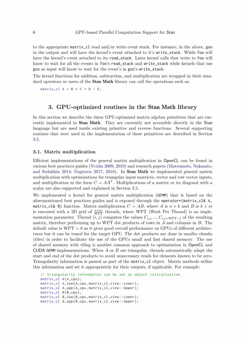
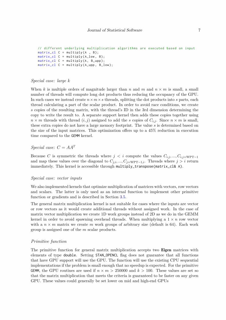
We implemented a general solver for Ax = b, where A is triangular and a special case whereb is an identity matrix. In the latter, we transfer the input matrix to the GPU, if notalready present in the GPUs global memory, and calculate the lower triangular inverse of Aon the GPU. If A is upper triangular the input and output of the lower triangular inverse aretransposed. The result is then copied back to the global memory of the host. The generalsolver only adds a multiplication of the inverse A−1 with the right-hand side b.The OpenCL implementation of the lower triangular inverse is based on our previous work(Češnovar and Štrumbelj 2017). The forward substitution algorithm that is commonly usedin sequential implementations is not suitable even for multi-core parallel implementations asit requires constant communication between threads. The communication-free algorithm formulti-core CPUs proposed in (Mahfoudhi, Mahjoub, and Nasri 2012) is based on the divide-and-conquer approach. The idea is that we can split the matrix into submatrices as shownin Figure 2. The input matrix is split in three submatrices: A1, A2 and A3. We calculatethe inverses of A1 and A2 in parallel to get C1 and C2. The remaining submatrix is thencalculated using C3 = −C2A3C1, with matrix multiplication also parallelized as shown inSection 3.1.Our approach generalizes this for many-core architectures, calculating a batch of smallerinverses along the diagonal in the first step (blocks labeled S1 in Figure 3). For this step weuse kernel batch_identity (see 3.5). It creates a large number of smaller identity matricesthat are then used in diag_inv to calculate the inverses of the smaller submatrices along thediagonal. For a n× n matrix, this kernel is executed with n threads split into b work groups,where b is the number of submatrices along the diagonal. Each work group is thus assignedone of the inverses along the diagonal. The rest of the submatrices are calculated by applying


Figure 2: Splitting into submatrices when computing the lower triangular inverse.

equation C3 = −C2A3C1. For Figure 3 this is done in four steps, first calculating submatriceslabeled S2, then reapplying the same equation to calculate submatrices S3, S4 and S5. Eachstep is done in two phases, first calculating T = C2A3 with the inv_lower_tri_multiply andthen C3 = −TC1 with the neg_rect_lower_tri_multiply kernel. Both kernels are based onthe general matrix multiply kernel but modified to handle a batch of multiplications of smallsubmatrices. The GPU support is only used when n > 500.

Figure 3: Splitting into submatrices when computing the lower triangular inverse.


In order to add GPU support to the reverse mode implementation of triangular system solvers,we used the lower triangular inverse kernel, the GEMM kernels, and the trivial transpose kernel.There are again three implementations for solving triangular systems in the form Ax = b, onewith A and b being matrices of var, and two cases where either of them is a matrix of doubles.In the function evaluation phase, we use the same principles as in the primitive function withthe added steps of extracting a matrix of doubles from the inputs, if needed. In the chain()function that is used to evaluate the gradient, we have three input matrices: adjC, A and C.To evaluate the gradient we calculate the following:

A * adjB = adjC;adjA = - adjB * C.transpose ();


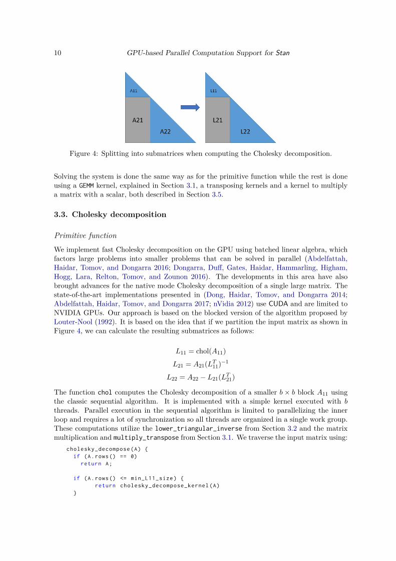
Figure 4: Splitting into submatrices when computing the Cholesky decomposition.

Solving the system is done the same way as for the primitive function while the rest is doneusing a GEMM kernel, explained in Section 3.1, a transposing kernels and a kernel to multiplya matrix with a scalar, both described in Section 3.5.

3.3. Cholesky decomposition

Primitive function

We implement fast Cholesky decomposition on the GPU using batched linear algebra, whichfactors large problems into smaller problems that can be solved in parallel (Abdelfattah,Haidar, Tomov, and Dongarra 2016; Dongarra, Duff, Gates, Haidar, Hammarling, Higham,Hogg, Lara, Relton, Tomov, and Zounon 2016). The developments in this area have alsobrought advances for the native mode Cholesky decomposition of a single large matrix. Thestate-of-the-art implementations presented in (Dong, Haidar, Tomov, and Dongarra 2014;Abdelfattah, Haidar, Tomov, and Dongarra 2017; nVidia 2012) use CUDA and are limited toNVIDIA GPUs. Our approach is based on the blocked version of the algorithm proposed byLouter-Nool (1992). It is based on the idea that if we partition the input matrix as shown inFigure 4, we can calculate the resulting submatrices as follows:

L11 = chol(A11)

L21 = A21(LT11)−1

L22 = A22 − L21(LT21)

The function chol computes the Cholesky decomposition of a smaller b × b block A11 usingthe classic sequential algorithm. It is implemented with a simple kernel executed with bthreads. Parallel execution in the sequential algorithm is limited to parallelizing the innerloop and requires a lot of synchronization so all threads are organized in a single work group.These computations utilize the lower_triangular_inverse from Section 3.2 and the matrixmultiplication and multiply_transpose from Section 3.1. We traverse the input matrix using:

cholesky_decompose(A) {if (A.rows() == 0)

return A;

if (A.rows() <= min_L11_size) {return cholesky_decompose_kernel(A)

}


block = A.rows() / partition

A_11 = A(0:block , 0:block)L_11 = cholesky_decompose(A_11);

A(0:block , 0:block) = L_11

block_subset = A.rows() - blockA_21 = A(block:A.rows(), 0:block)L_21 = A_21 * transpose(lower_triangular_inverse(L_11))A(block:A.rows(), 0:block) = L_21

A_22 = A(block:A.rows(), block:A.rows ())

L_22 = A_22 - multiply_transpose(L_21)

L_rem_11 = cholesky_decompose(L_22);A(block:N, block:N) = L_rem_11return A;

}

Note that partition and min_L11_size are implementation parameters.


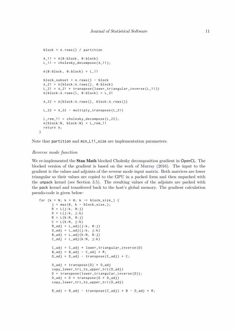
We re-implemented the Stan Math blocked Cholesky decomposition gradient in OpenCL. Theblocked version of the gradient is based on the work of Murray (2016). The input to thegradient is the values and adjoints of the reverse mode input matrix. Both matrices are lowertriangular so their values are copied to the GPU in a packed form and then unpacked withthe unpack kernel (see Section 3.5). The resulting values of the adjoints are packed withthe pack kernel and transferred back to the host’s global memory. The gradient calculationpseudo-code is given below:

for (k = N; k > 0; k -= block_size_) {j = max(0, k - block_size_ );R = L(j:k, 0:j)D = L(j:k, j:k)B = L(k:N, 0:j)C = L(k:N, j:k)R_adj = L_adj(j:k, 0:j)D_adj = L_adj(j:k, j:k)B_adj = L_adj(k:N, 0:j)C_adj = L_adj(k:N, j:k)

C_adj = C_adj * lower_triangular_inverse(D)B_adj = B_adj - C_adj * R;D_adj = D_adj - transpose(C_adj) * C;

D_adj = transpose(D) * D_adjcopy_lower_tri_to_upper_tri(D_adj)D = transpose(lower_triangular_inverse(D));D_adj = D * transpose(D * D_adj)copy_lower_tri_to_upper_tri(D_adj)

R_adj = R_adj - transpose(C_adj) * B - D_adj * R;


●●● ●●● ●●●

●

●●●●●

●●

●

●

●

●

●

●

●

●

●

●

●

●

●

●

●

●

●●● ●●●

●●●

●●●

●●●

●

●●

●

●●

●

●●

●

●

●

●

●

●

●●● ●●● ●

●● ●●●●●●

●●●

●●●

●

●●

●

●●

●

●●

cholesky_decompose_double cholesky_decompose_grad cholesky_decompose_var

0 5000 10000 0 5000 10000 0 5000 10000

0

10

20

30

40

n

spee

dup

GPU ● ● ●radeon titanxp v100

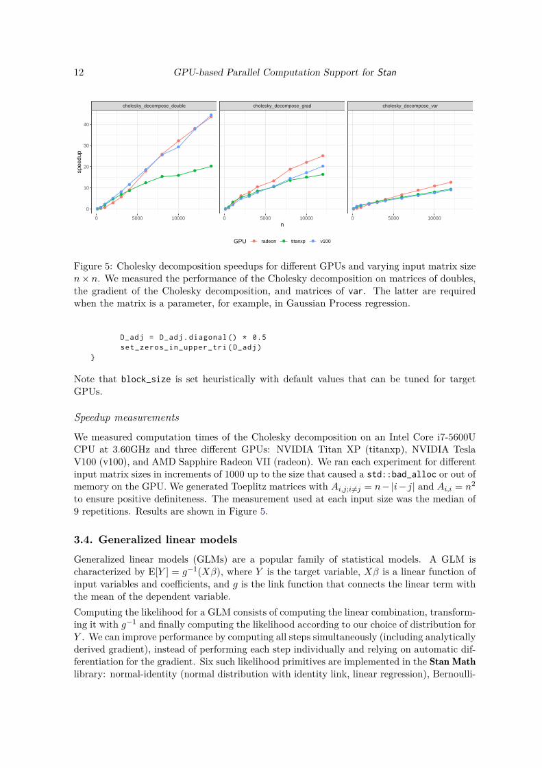
Figure 5: Cholesky decomposition speedups for different GPUs and varying input matrix sizen× n. We measured the performance of the Cholesky decomposition on matrices of doubles,the gradient of the Cholesky decomposition, and matrices of var. The latter are requiredwhen the matrix is a parameter, for example, in Gaussian Process regression.

D_adj = D_adj.diagonal () * 0.5set_zeros_in_upper_tri(D_adj)

}

Note that block_size is set heuristically with default values that can be tuned for targetGPUs.

Speedup measurements

We measured computation times of the Cholesky decomposition on an Intel Core i7-5600UCPU at 3.60GHz and three different GPUs: NVIDIA Titan XP (titanxp), NVIDIA TeslaV100 (v100), and AMD Sapphire Radeon VII (radeon). We ran each experiment for differentinput matrix sizes in increments of 1000 up to the size that caused a std::bad_alloc or out ofmemory on the GPU. We generated Toeplitz matrices with Ai,j;i 6=j = n−|i− j| and Ai,i = n2

to ensure positive definiteness. The measurement used at each input size was the median of9 repetitions. Results are shown in Figure 5.

3.4. Generalized linear models

Generalized linear models (GLMs) are a popular family of statistical models. A GLM ischaracterized by E[Y ] = g−1(Xβ), where Y is the target variable, Xβ is a linear function ofinput variables and coefficients, and g is the link function that connects the linear term withthe mean of the dependent variable.Computing the likelihood for a GLM consists of computing the linear combination, transform-ing it with g−1 and finally computing the likelihood according to our choice of distribution forY . We can improve performance by computing all steps simultaneously (including analyticallyderived gradient), instead of performing each step individually and relying on automatic dif-ferentiation for the gradient. Six such likelihood primitives are implemented in the Stan Mathlibrary: normal-identity (normal distribution with identity link, linear regression), Bernoulli-


logit (logistic regression), Poisson-log, negative binomial-log, categorical-logit (multinomiallogistic regression), and ordinal-logit (ordinal logistic regression). Stan users can access themby calling the built-in log-pdf/pmf. These likelihoods can also be used as components in morecomplex models, such as multi-level regression.Note that the GLM likelihoods are heavily templated. With the exception of integers, everyargument can have type var or double. Many arguments can either be scalars or vectors. Forexample, standard deviation in the normal-identity GLM can be the usual scalar parameteror, if we want to implement heteroskedasticity, a vector.The GPU implementation of the GLM primitives is based on their CPU implementation thatis already in Stan and not part of this work. First, the data are transferred to the GPU. Theargument types also determine which derivatives we need to compute. This information istransferred to the GPU kernel by kernel arguments and it allows kernels to skip unnecessarycomputation.Each GLM is implemented in a single kernel. The kernel requires execution of one threadper input variable. The number of threads is rounded up and they are organized into workgroups of size 64. Each thread calculates one scalar product of the matrix-vector productand additional GLM-specific values and derivatives. Computation of the (log) likelihood endswith the summation over intermediate values, computed by each thread. Threads in a workgroup execute parallel reduction. First thread of each work group writes partial sum to theglobal memory. Partial sums are then transferred to the main memory and summation iscompleted by the CPU.Derivatives with respect to coefficients and input variables require calculation of anothermatrix-vector product. Since another product cannot be efficiently computed in the samekernel, a GEMV kernel is run if these derivatives are needed.

3.5. Supporting GPU routines

Here we describe additional OpenCL kernels that are available in Stan Math. These routinesare not bottlenecks of statistical computation, so we opted for simplicity. All kernels use thedefault work group size determined by OpenCL.These OpenCL kernels often do not outperform their CPU or Eigen equivalents, especiallywhen we consider data transfers to or from the OpenCL GPU device. They should only beused as parts of an algorithm or when there is no data copy overhead. Note that all OpenCLkernels in Stan Math can be used as building blocks for new GPU routines.All the kernels below assume input matrices of size m×n.

Add and subtract

These kernels add or subtract two matrices of the same size and store the result to a thirdmatrix buffer. They execute on a grid of m×n threads, where thread (i, j) adds or subtractselements Ai,j and Bi,j and stores them to Ci,j .The kernel code for adding two matrices:

__kernel void add(__global double *C, __global double *A,__global double *B, unsigned int rows ,unsigned int cols) {

int i = get_global_id (0);


int j = get_global_id (1);if (i < rows && j < cols) {

C(i, j) = A(i, j) + B(i, j);}

}

Multiplication with scalar

Kernels scalar_mul and scalar_mul_diagonal can be used to multiply a matrix with a scalar.The former multiplies the entire input matrix with the given scalar while the latter multipliesonly the diagonal elements. Similarly to the add and subtract kernels, the kernel scalar_mulis executed with m×n threads with each thread multiplying one matrix element. The kernelscalar_mul_diagonal is executed with min(m,n) threads with each thread multiplying onediagonal element.

Matrix transpose

Two kernels can be used for transposing a matrix and both are executed withm×n threads. Inkernel transpose each thread copies an element from Ai,j to Bj,i and triangular_transposecopies the lower triangular of a matrix to the upper triangular or vice-versa. In the formercase, the threads with indices under and on the diagonal perform Aj,i = Ai,j and threadsabove the diagonal do nothing. In the latter case the roles are reversed.

Matrix initialization

Three kernels can be used to initialize a matrix: zeros, identity and batch_identity. Forkernel zeros we specify the output matrix, its size, and if we want to set zeros only onthe lower or upper triangular of the matrix. In both cases, we spawn m × n threads, witheach thread assigned a single matrix element. Similarly, for kernel identity each thread isassigned a single matrix element. The batch_identity kernel is used to make a batch ofsmaller identity matrices in a single continuous buffer. This kernel is executed with k×n×nthreads, where k is the number of n× n identity matrices to create. Each thread is assigneda single element in one of the batch matrices, with the thread ID (0, ..., k − 1) on the firstdimension determining the matrix and the IDs on the remaining two dimensions determiningthe element of the matrix.

Submatrix copy

OpenCL provides functions that enable copying of entire matrix buffers. In order to add thefunctionality of copying arbitrary submatrices we implemented the sub_block kernel. Thiskernel copies a rectangular or triangular submatrix of size k × l from a source matrix to agiven submatrix of the destination matrix of size m × n. Each of the k × l threads thatexecute this kernel is assigned one element of the submatrix. The thread then determineswhether to copy the element based on the triangular view argument and its indices on thetwo dimensions. Similarly to the zeros kernel, sub_block has a triangular view argumentthat determines whether to copy the entire input matrix or only the lower/upper triangularparts.


Input checking

We implemented kernels that allow the user to check whether the matrices stored on theOpenCL devices are symmetric, contain NaN values or contain zeros on the diagonal. Theinputs are a pointer to the matrix buffer, its size and a pointer to a flag variable. If theconditions of the check are met, the matrix sets the flag. No threads reset the flag so thereare no race conditions. check_diagonal_zeros is executed with min(m,n) threads, eachthread checking one diagonal element for zeros. check_nan is executed with m × n threads,each thread checking one matrix element for NaN. For the kernel check_symmetric the flagshould be set before executing the kernel with the threads resetting it upon discovery of non-symmetry. The kernel is again executed using m× n threads, each thread checking whetherAi,j −Aj,i is within tolerance of zero.

3.6. Kernel fusion

If only the basic computation primitives are implemented for the GPU, we are faced with adilemma when developing new algorithms that are a composition of these primitives (for ex-ample, GLM likelihoods). We can call multiple kernels or manually develop a new kernel thatcombines multiple primitive methods into a single kernel. The latter speeds up computationin two ways. First, we reduce kernel launch overhead. And second, we reduce the amountof memory transfers. Combining kernels is also referred to as kernel fusion (Filipovič andBenkner 2015) and it can be done manually or automated.The problem with manually developing new kernels is that it requires specific expertise and isa time consuming process. To mitigate this, we also developed an OpenCL GPU kernel fusionlibrary for Stan Math. The library automatically combines kernels, optimizes computation,and is simple to use. This speeds up the development of new GPU kernels while keepingthe performance of automatically combined kernels comparable to hand crafted kernels. Thedetails of the kernel fusion library for Stan Math can be found in Ciglarič, Češnovar, andŠtrumbelj (2020).We maintain a list of functions that are implemented and available for use with the ker-nel generator at https://github.com/bstatcomp/math/issues/15. It includes the previouslymentioned add and subtract, multiplication with scalar, and submatrix copy.

4. Illustrative examplesIn this section we show two illustrative examples that demonstrate the use of the new GPUroutines and what speedups we can expect.

• The measurements are end-to-end, measuring the speedups that a user would experienceduring typical use. That is, we measure the time it takes from calling the model tosample to when the samples are output by the model. This includes reading the data andoutputting the samples, but not model compilation time. Model compilation only hasto be done once and we find it reasonable to assume that compilation time is negligibleover the life span of the model. For logistic regression we ran each experiment for 500warmup and 500 sampling iterations and for GP regression 30 warmup and 10 samplingiterations.

https://github.com/bstatcomp/math/issues/15


• We made three measurements for each hardware-model-input size configuration. Wecalculate speedups by dividing the average of the three measurements for the devicewith the average of the three measurements for the reference device (cpu).

• We ran the experiments on an Intel Core i7-5600U CPU (cpu) at 3.60GHz and twodifferent GPUs: NVIDIA Titan XP (titanxp), and AMD Sapphire Radeon VII (radeon).

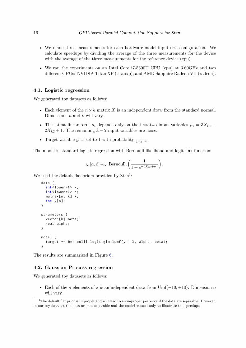
4.1. Logistic regression

We generated toy datasets as follows:

• Each element of the n× k matrix X is an independent draw from the standard normal.Dimensions n and k will vary.

• The latent linear term µi depends only on the first two input variables µi = 3Xi,1 −2Xi,2 + 1. The remaining k − 2 input variables are noise.

• Target variable yi is set to 1 with probability 11+e−µi .

The model is standard logistic regression with Bernoulli likelihood and logit link function:

yi|α, β ∼iid Bernoulli( 1

1 + e−(Xiβ+α)

).

We used the default flat priors provided by Stan1:data {

int <lower=1> k;int <lower=0> n;matrix[n, k] X;int y[n];

}

parameters {vector[k] beta;real alpha;

}

model {target += bernoulli_logit_glm_lpmf(y | X, alpha , beta);

}

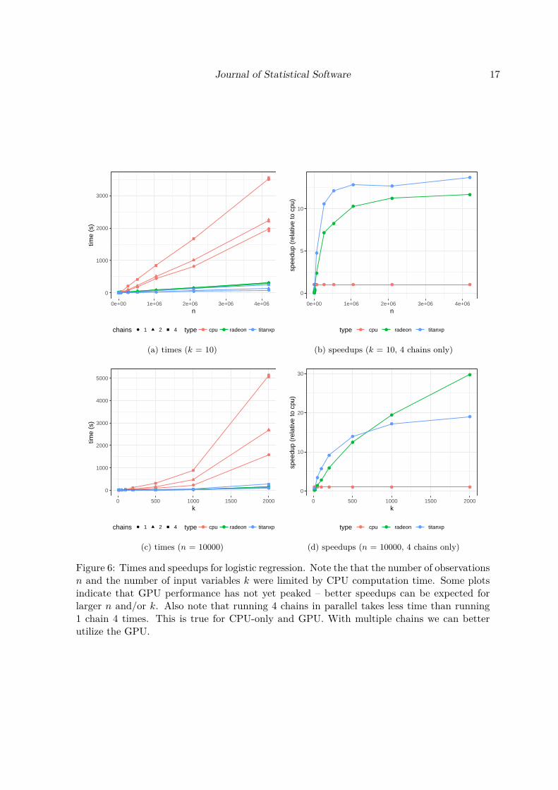
The results are summarized in Figure 6.

4.2. Gaussian Process regression

We generated toy datasets as follows:

• Each of the n elements of x is an independent draw from Unif(−10,+10). Dimension nwill vary.

1The default flat prior is improper and will lead to an improper posterior if the data are separable. However,in our toy data set the data are not separable and the model is used only to illustrate the speedups.


●●●●●●●●●●●●●●●●●●●●●●●●●●●●●●●●●●●●●●●●●●

●●●

●●●

●●●

●●●

●●●

●●●

●●●

●●●

●●●●●●●●●●●●●●●●●●●●●●●●●●●●●● ●●● ●●● ●●● ●●● ●●●●●●●0

1000

2000

3000

0e+00 1e+06 2e+06 3e+06 4e+06n

time

(s)

chains ● 1 2 4 type ● ● ●cpu radeon titanxp

(a) times (k = 10)

●

●●

●

●●

●

●●

●

●●

●

●●

●

●

●●●●

●

●

●

●

●

●

●

●

●

●

●

●

●

●

●

●

●

0

5

10

0e+00 1e+06 2e+06 3e+06 4e+06n

spee

dup

(rel

ativ

e to

cpu

)

type ● ● ●cpu radeon titanxp

(b) speedups (k = 10, 4 chains only)

●●●●●●●●●●●●●●●●●● ●●●●●● ●●●●●●●●●●●●

●●●

●●●

●●●

●●●●●●●●●●●● ●●● ●●● ●●● ●●●

●●●0

1000

2000

3000

4000

5000

0 500 1000 1500 2000k

time

(s)

chains ● 1 2 4 type ● ● ●cpu radeon titanxp

(c) times (n = 10000)

●●●●●●●●

●

●

●

●

●

●

●

●

●

●

●

●

●

●

●

●

0

10

20

30

0 500 1000 1500 2000k

spee

dup

(rel

ativ

e to

cpu

)

type ● ● ●cpu radeon titanxp

(d) speedups (n = 10000, 4 chains only)

Figure 6: Times and speedups for logistic regression. Note the that the number of observationsn and the number of input variables k were limited by CPU computation time. Some plotsindicate that GPU performance has not yet peaked – better speedups can be expected forlarger n and/or k. Also note that running 4 chains in parallel takes less time than running1 chain 4 times. This is true for CPU-only and GPU. With multiple chains we can betterutilize the GPU.


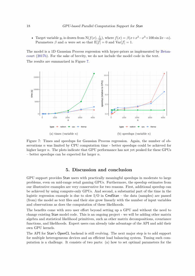
• Target variable yi is drawn from N(f(x), 110), where f(x) = β(x+x2−x3+100 sin 2x−α).

Parameters β and α were set so that E[f ] = 0 and Var[f ] = 1.

The model is a 1D Gaussian Process regression with hyper-priors as implemented by Betan-court (2017b). For the sake of brevity, we do not include the model code in the text.The results are summarized in Figure 7.

●●●●●●●●●●●● ●●● ●●● ●●●●●●

●●● ●●●

●●●●●●●●●●●● ●●● ●●● ●●●

●●●

●●●

●●●

●●●●●●●●●●●● ●●● ●●● ●●●●●●

●●●

●●●

0

5000

10000

15000

0 1000 2000 3000 4000n

time

(s)

type ● ● ●radeon cpu titanxp

(a) times (variable n)

●

●

●

●

●

●

●

●

●

●

●●

●

●●

●●

●●

●

●●

●

●

●

●

●

●

●

●

0.0

2.5

5.0

7.5

10.0

0 1000 2000 3000 4000n

spee

dup

(rel

ativ

e to

CP

U)

type ● ● ●radeon cpu titanxp

(b) speedups (variable n)

Figure 7: Times and speedups for Gaussian Process regression. Again, the number of ob-servations n was limited by CPU computation time - better speedups could be achieved forhigher larger n. The plots indicate that GPU performance has not yet peaked for these GPUs– better speedups can be expected for larger n.

5. Discussion and conclusionGPU support provides Stan users with practically meaningful speedups in moderate to largeproblems, even on mid-range retail gaming GPUs. Furthermore, the speedup estimates fromour illustrative examples are very conservative for two reasons. First, additional speedup canbe achieved by using compute-only GPUs. And second, a substantial part of the time in thelogistic regression example is due to slow I/O in CmdStan – the data (samples) are passed(from) the model as text files and their size grow linearly with the number of input variablesand observations as does the computation of these likelihoods.The benefits come with zero user effort beyond setting up a GPU and without the need tochange existing Stan model code. This is an ongoing project - we will be adding other matrixalgebra and statistical likelihood primitives, such as other matrix decompositions, covariancefunctions, and likelihoods. Expert users can already take advantage of the API and add theirown GPU kernels.The API for Stan’s OpenCL backend is still evolving. The next major step is to add supportfor multiple heterogeneous devices and an efficient load balancing system. Tuning such com-putation is a challenge. It consists of two parts: (a) how to set optimal parameters for the


device(s) and (b) when to move computation to the device(s) (when does the speedup justifythe overhead). The iterative Markov Chain Monte Carlo (or optimization) setting lends itselfto the possibility of efficient online tuning, because computation and input dimensions areconstant over all iterations.

Computational detailsAll the functionality described in this paper is part of Stan as of releases CmdStan 2.22 andStan Math 3.1.Instructions on how to activate GPU support for CmdStan or CmdStanR can be found here:https://github.com/bstatcomp/stan_gpu_install_docs

AcknowledgmentsWe would like to thank Bob Carpenter for for his comments on an earlier draft of our work.This research was supported by the Slovenian Research Agency (ARRS, project grant L1-7542 and research core funding P5-0410). We gratefully acknowledge the support of NVIDIACorporation with the donation of the Titan XP GPU used for this research. We gratefully ac-knowledge the support of Amazon with an Amazon Research Award. Part of Steve Bronder’scontributions were made while he was working at Capital One.

References

Abdelfattah A, Haidar A, Tomov S, Dongarra J (2016). “Performance Tuning and Op-timization Techniques of Fixed and Variable Size Batched Cholesky Factorization onGPUs.” Procedia Computer Science, 80, 119 – 130. ISSN 1877-0509. doi:https://doi.org/10.1016/j.procs.2016.05.303. International Conference on ComputationalScience 2016, ICCS 2016, 6-8 June 2016, San Diego, California, USA, URL http://www.sciencedirect.com/science/article/pii/S1877050916306548.

Abdelfattah A, Haidar A, Tomov S, Dongarra J (2017). “Fast Cholesky Factorization onGPUs for Batch and Native Modes in MAGMA.” Journal of Computational Science, 20, 85– 93. ISSN 1877-7503. doi:https://doi.org/10.1016/j.jocs.2016.12.009. URL http://www.sciencedirect.com/science/article/pii/S1877750316305154.

Baudart G, Hirzel M, Mandel L (2018). “Deep Probabilistic Programming Languages: AQualitative Study.” arXiv preprint arXiv:1804.06458.

Bergstra J, Breuleux O, Bastien F, Lamblin P, Pascanu R, Desjardins G, Turian J, Warde-Farley D, Bengio Y (2010). “Theano: a CPU and GPU Math Expression Compiler.” InProceedings of the Python for scientific computing conference (SciPy), volume 4. Austin,TX.

Betancourt M (2017a). “A conceptual introduction to Hamiltonian Monte Carlo.” arXivpreprint arXiv:1701.02434.

https://github.com/bstatcomp/stan_gpu_install_docs

http://dx.doi.org/https://doi.org/10.1016/j.procs.2016.05.303

http://dx.doi.org/https://doi.org/10.1016/j.procs.2016.05.303

http://www.sciencedirect.com/science/article/pii/S1877050916306548


http://dx.doi.org/https://doi.org/10.1016/j.jocs.2016.12.009




Betancourt M (2017b). “Robust Gaussian Processes in Stan, Part 3.” Retrieved from https://betanalpha.github.io/assets/case_studies/gp_part3/part3.html.

Bingham E, Chen JP, Jankowiak M, Obermeyer F, Pradhan N, Karaletsos T, Singh R, SzerlipP, Horsfall P, Goodman ND (2019). “Pyro: Deep Universal Probabilistic Programming.”The Journal of Machine Learning Research, 20(1), 973–978.

Bürkner PC, et al. (2017). “brms: An R Package for Bayesian Multilevel Models Using Stan.”Journal of Statistical Software, 80(1), 1–28.

Carpenter B, Gelman A, Hoffman MD, Lee D, Goodrich B, Betancourt M, Brubaker M, GuoJ, Li P, Riddell A (2017). “Stan: A Probabilistic Programming Language.” Journal ofStatistical Software, 76(i01).

Češnovar R, Štrumbelj E (2017). “Bayesian Lasso and Multinomial Logistic Regression onGPU.” PLoS ONE, 12(6), e0180343.

Ciglarič T, Češnovar R, Štrumbelj E (2020). “Automated OpenCL GPU kernel fusion forStan Math.” In Proceedings of the International Workshop on OpenCL, pp. 1–6.

Dong T, Haidar A, Tomov S, Dongarra J (2014). “A Fast Batched Cholesky Factorization ona GPU.” In 2014 43rd International Conference on Parallel Processing, pp. 432–440. ISSN0190-3918. doi:10.1109/ICPP.2014.52.

Dongarra JJ, Duff I, Gates M, Haidar A, Hammarling S, Higham NJ, Hogg J, Lara P, ReltonSD, Tomov S, Zounon M (2016). “A Proposed API for Batched Basic Linear AlgebraSubprograms.”

Filipovič J, Benkner S (2015). “OpenCL kernel fusion for GPU, Xeon Phi and CPU.” In 201527th International Symposium on Computer Architecture and High Performance Computing(SBAC-PAD), pp. 98–105. IEEE.

Gabry J, Goodrich B (2016). “rstanarm: Bayesian Applied Regression Modeling via Stan.”R package version, 2(1).

Guennebaud G, Jacob B, et al. (2010). “Eigen v3.” http://eigen.tuxfamily.org.

Hoffman MD, Gelman A (2014). “The No-U-turn Sampler: Adaptively Setting Path Lengthsin Hamiltonian Monte Carlo.” Journal of Machine Learning Research, 15(1), 1593–1623.

Louter-Nool M (1992). “Block-Cholesky for Parallel Processing.” Appl. Numer. Math., 10(1),37–57. ISSN 0168-9274. doi:10.1016/0168-9274(92)90054-H. URL http://dx.doi.org/10.1016/0168-9274(92)90054-H.

Mahfoudhi R, Mahjoub Z, Nasri W (2012). “Parallel Communication-Free Algorithm forTriangular Matrix Inversion on Heterogenoues Platform.” In 2012 Federated Conference onComputer Science and Information Systems (FedCSIS), pp. 553–560.

Matsumoto K, Nakasato N, Sedukhin SG (2014). “Implementing Level-3 BLAS Routines inOpenCL on Different Processing Units.”

Murray I (2016). “Differentiation of the Cholesky Decomposition.” arXiv e-prints,arXiv:1602.07527. 1602.07527.

https://betanalpha.github.io/assets/case_studies/gp_part3/part3.html

https://betanalpha.github.io/assets/case_studies/gp_part3/part3.html

http://dx.doi.org/10.1109/ICPP.2014.52

http://dx.doi.org/10.1016/0168-9274(92)90054-H

http://dx.doi.org/10.1016/0168-9274(92)90054-H

http://dx.doi.org/10.1016/0168-9274(92)90054-H

1602.07527


Nugteren C (2017). “CLBlast: A Tuned OpenCL BLAS Library.” CoRR, abs/1705.05249.1705.05249, URL http://arxiv.org/abs/1705.05249.

Nugteren C (2018). “CLBlast: A Tuned OpenCL BLAS Library.” In Proceedings of the In-ternational Workshop on OpenCL, IWOCL ’18, pp. 5:1–5:10. ACM, New York, NY, USA.ISBN 978-1-4503-6439-3. doi:10.1145/3204919.3204924. URL http://doi.acm.org/10.1145/3204919.3204924.

Nvidia (2009). “NVIDIA OpenCL Best Practices Guide .”

Nvidia (2010). “NVIDIA CUDA C Programming Guide.”

nVidia (2012). CUBLAS Library User Guide. nVidia, v5.0 edition. URL http://docs.nvidia.com/cublas/index.html.

Paszke A, Gross S, Chintala S, Chanan G, Yang E, DeVito Z, Lin Z, Desmaison A, Antiga L,Lerer (2017). “Automatic Differentiation in PyTorch.” In NIPS Autodiff Workshop.

Salvatier J, Wiecki TV, Fonnesbeck C (2016). “Probabilistic Programming in Python usingPyMC3.” PeerJ Computer Science, 2, e55.

Stan Development Team (2020). Stan Modeling Language User’s Guide and Reference Man-ual, Version 2.22. URL http://mc-stan.org/.

Stone JE, Gohara D, Shi G (2010). “OpenCL: A Parallel Programming Standard for Het-erogeneous Computing Systems.” IEEE Des. Test, 12(3), 66–73. ISSN 0740-7475. doi:10.1109/MCSE.2010.69. URL http://dx.doi.org/10.1109/MCSE.2010.69.

Taylor SJ, Letham B (2018). “Forecasting at Scale.” The American Statistician, 72(1), 37–45.

Tran D, Hoffman MD, Saurous RA, Brevdo E, Murphy K, Blei DM (2017). “Deep Proba-bilistic Programming.” arXiv preprint arXiv:1701.03757.

Van Heesch D (2008). “Doxygen: Source Code Documentation Generator Tool.” URL:http://www. doxygen. org.

Zheng, Chen T, Li M, Li Y, Lin M, Wang N, Wang M, Xiao T, Xu B, Zhang C, Zhang (2015).“Mxnet: A Flexible and Efficient Machine Learning Library for Heterogeneous DistributedSystems.” arXiv preprint arXiv:1512.01274.

1705.05249

http://arxiv.org/abs/1705.05249

http://dx.doi.org/10.1145/3204919.3204924

http://doi.acm.org/10.1145/3204919.3204924

http://doi.acm.org/10.1145/3204919.3204924

http://docs.nvidia.com/cublas/index.html

http://docs.nvidia.com/cublas/index.html

http://mc-stan.org/

http://dx.doi.org/10.1109/MCSE.2010.69




Affiliation:Rok Češnovar, Davor Sluga, Jure Demšar, Tadej Ciglarič, Erik ŠtrumbeljUniversity of LjubljanaFaculty of Computer and Information ScienceE-mail: [email protected] BronderISERPColumbia UniversityE-mail: [email protected] TaltsISERPColumbia UniversityE-mail: [email protected]

mailto:[email protected]



Documents

GPU-based Parallel Computation Support for Stan · Stan has three distinct components: a probabilistic programming language, the Stan Math librarythatsupportsauto-diﬀerentiation,andalgorithmsforinference