FACULTYFACULTYFACULTYFACULTYOFOFOFOF ENGINEERINGENGINEERINGENGINEERINGENGINEERINGANDANDANDANDSUSTAINABLESUSTAINABLESUSTAINABLESUSTAINABLEDEVELOPMENTDEVELOPMENTDEVELOPMENTDEVELOPMENT

A study of the possibility to connect local levellingnetworks to the Swedish height system RH 2000

using GNSS

Ke Liu

MayMayMayMay 2011201120112011

ThesisThesisThesisThesis forforforfor aaaa DegreeDegreeDegreeDegree ofofofofMasterMasterMasterMaster ofofofof ScienceScienceScienceScience inininin GeomaticsGeomaticsGeomaticsGeomaticsSupervisor:Supervisor:Supervisor:Supervisor: MartinMartinMartinMartin LidbergLidbergLidbergLidberg

Examiner:Examiner:Examiner:Examiner: Stig-GStig-GStig-GStig-GööööranranranranMMMMåååårtenssonrtenssonrtenssonrtensson

I

AbstractAbstractAbstractAbstractIn this study, the connection of a local levelling network to thenational height system in Sweden, RH 2000, with GNSS-techniques isinvestigated. The SWEN 08 is applied as geoid model. Essentially,the method is precise normal height determination with GNSS. Theaccuracy, repeatability and the affecting elements are tested.According to the statistics, the proposed method achieves 1-cmaccuracy level. Suggestions on the general methodology and settingsof several elements are proposed based on the statistics for the futureapplication.

KeywordsKeywordsKeywordsKeywords::::GNSS, GPS, levelling, RH 2000

II

PrefacePrefacePrefacePreface

This thesis is a MSc diploma work by Ke Liu, who studies Geomaticsat the University of Gävle (Högskolan i Gävle, HiG), Sweden. Thisstudy is performed for and conducted by Lantmäteriet – the Swedishmapping, cadastral and land registration authority. Lantmäterietprovides the data and software, on which this study is based.

Martin Lidberg at Lantmäteriet and Stig-Göran Mårtensson at theUniversity of Gävle offered me this precious chance to undertakesuch study, provided crucial and kindly help. Tina Kempe calculatedanother table of statistics separately, helped a lot with patient on themethod. This study could not have been accomplished without theirkindness, patient and professional guidance. I sincerely express mygratitude to Martin, Stig-Göran, Tina, as well as everybody whocared and contributed to this study.

III

AbstractAbstractAbstractAbstract iiii

PrefacePrefacePrefacePreface iiiiiiii

1111 IntroductionIntroductionIntroductionIntroduction 11111.11.11.11.1 RRRRevieweviewevieweview onononon formerformerformerformer studiesstudiesstudiesstudies 33331.21.21.21.2 AimAimAimAim andandandand objectivesobjectivesobjectivesobjectives 4444

2222 TheTheTheThe GNSSGNSSGNSSGNSS fieldfieldfieldfield experimentexperimentexperimentexperiment 55552.12.12.12.1 TheTheTheThe choicechoicechoicechoice ofofofof studystudystudystudy areaareaareaarea 55552.22.22.22.2 GPSGPSGPSGPS campaignscampaignscampaignscampaigns 7777

3333 TheTheTheThemmmmethodethodethodethod ofofofof connectingconnectingconnectingconnecting locallocallocallocal levellinglevellinglevellinglevellingnetworksnetworksnetworksnetworks totototo RHRHRHRH 2000200020002000 9999

3.13.13.13.1 BaselinesBaselinesBaselinesBaselines processingprocessingprocessingprocessing andandandand networknetworknetworknetwork adjustmentadjustmentadjustmentadjustment 101010103.23.23.23.2 CoordinateCoordinateCoordinateCoordinate systemsystemsystemsystem transformationstransformationstransformationstransformations andandandand normalnormalnormalnormal heightheightheightheight

calculationscalculationscalculationscalculations 121212123.33.33.33.3 NetworkNetworkNetworkNetwork constraintconstraintconstraintconstraint andandandand GNSSGNSSGNSSGNSS obtainedobtainedobtainedobtained normalnormalnormalnormal heightsheightsheightsheights

correctioncorrectioncorrectioncorrection 131313133.43.43.43.4 HeightHeightHeightHeight computationcomputationcomputationcomputation ofofofof thethethethe otherotherotherother sitessitessitessites inininin thethethethe locallocallocallocal networknetworknetworknetwork14141414

4444 EvaluatiEvaluatiEvaluatiEvaluationononon ofofofof thethethethe proposedproposedproposedproposedmethodmethodmethodmethod 161616164.14.14.14.1 DesignDesignDesignDesign ofofofof experimentsexperimentsexperimentsexperiments 161616164.24.24.24.2 CheckCheckCheckCheck withwithwithwith knownknownknownknown networknetworknetworknetwork 191919194.34.34.34.3 StatisticsStatisticsStatisticsStatistics onononon thethethethe accuracyaccuracyaccuracyaccuracy 20202020

5555 ResultResultResultResult andandandand analysisanalysisanalysisanalysis 252525255.15.15.15.1 SomeSomeSomeSome explanationexplanationexplanationexplanation onononon thethethethe tablestablestablestables ofofofof resultresultresultresult 313131315.25.25.25.2 TheTheTheThe overalloveralloveralloverall accuracyaccuracyaccuracyaccuracy 313131315.35.35.35.3 AccuracyAccuracyAccuracyAccuracy withwithwithwith regardsregardsregardsregards totototo differentdifferentdifferentdifferent factorsfactorsfactorsfactors 323232325.45.45.45.4 AnalysisAnalysisAnalysisAnalysis onononon PossiblePossiblePossiblePossible ErrorErrorErrorError SourcesSourcesSourcesSources 47474747

6666 ConclusionConclusionConclusionConclusion andandandandDiscussionDiscussionDiscussionDiscussion 494949496.16.16.16.1 ConclusionConclusionConclusionConclusion 494949496.26.26.26.2 DiscussionDiscussionDiscussionDiscussion 50505050

TableTableTableTable ofofofof contentscontentscontentscontents

IV

7777 AcknowledgementsAcknowledgementsAcknowledgementsAcknowledgements 54545454

ReferencesReferencesReferencesReferences iiii

AppendixAppendixAppendixAppendix iiiiiiiiiiii1.1.1.1. InstallingInstallingInstallingInstalling thethethethe antennaantennaantennaantenna modelsmodelsmodelsmodels iiiiiiiiiiii2.2.2.2. RoutineRoutineRoutineRoutine ofofofof thethethethe ExcelExcelExcelExcel VBAVBAVBAVBAmacromacromacromacro usedusedusedused forforforfor statisticsstatisticsstatisticsstatistics vvvv

1

AAAA studystudystudystudy ofofofof thethethethe possibilitypossibilitypossibilitypossibility totototo connectconnectconnectconnectlocallocallocallocal levellinglevellinglevellinglevelling networksnetworksnetworksnetworks totototo thethethetheSwedishSwedishSwedishSwedish heightheightheightheight systemsystemsystemsystem RH2000RH2000RH2000RH2000

usingusingusingusing GNSSGNSSGNSSGNSS

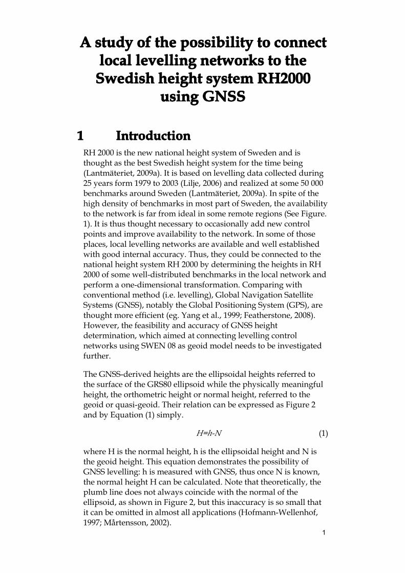
1111 IntroductionIntroductionIntroductionIntroductionRH 2000 is the new national height system of Sweden and isthought as the best Swedish height system for the time being(Lantmäteriet, 2009a). It is based on levelling data collected during25 years form 1979 to 2003 (Lilje, 2006) and realized at some 50 000benchmarks around Sweden (Lantmäteriet, 2009a). In spite of thehigh density of benchmarks in most part of Sweden, the availabilityto the network is far from ideal in some remote regions (See Figure.1). It is thus thought necessary to occasionally add new controlpoints and improve availability to the network. In some of thoseplaces, local levelling networks are available and well establishedwith good internal accuracy. Thus, they could be connected to thenational height system RH 2000 by determining the heights in RH2000 of some well-distributed benchmarks in the local network andperform a one-dimensional transformation. Comparing withconventional method (i.e. levelling), Global Navigation SatelliteSystems (GNSS), notably the Global Positioning System (GPS), arethought more efficient (eg. Yang et al., 1999; Featherstone, 2008).However, the feasibility and accuracy of GNSS heightdetermination, which aimed at connecting levelling controlnetworks using SWEN 08 as geoid model needs to be investigatedfurther.

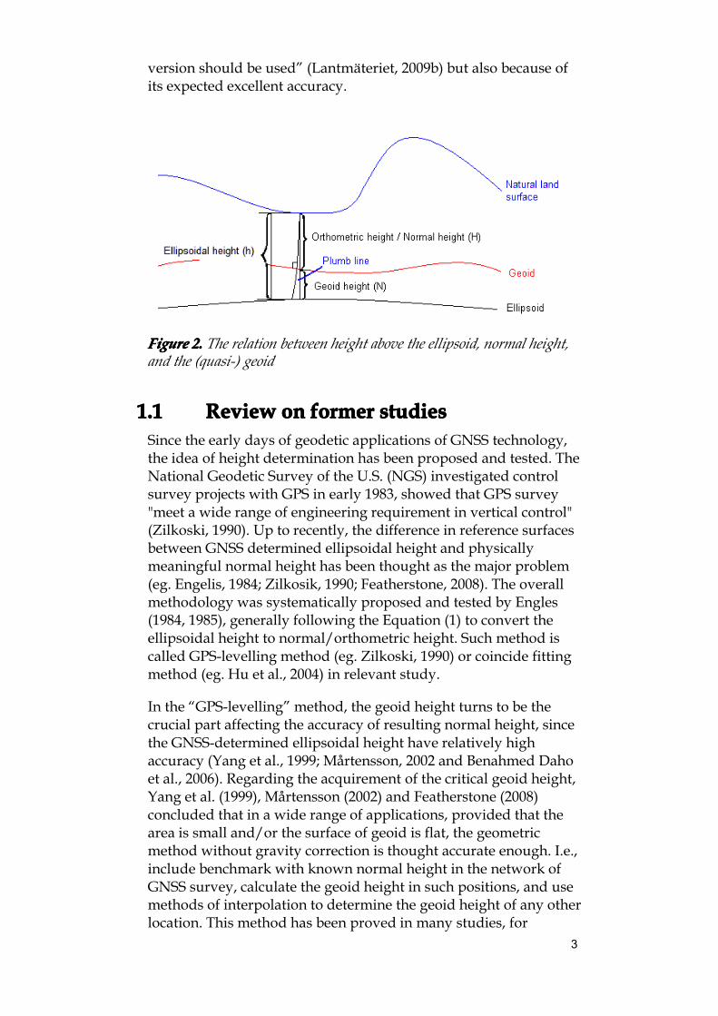
The GNSS-derived heights are the ellipsoidal heights referred tothe surface of the GRS80 ellipsoid while the physically meaningfulheight, the orthometric height or normal height, referred to thegeoid or quasi-geoid. Their relation can be expressed as Figure 2and by Equation (1) simply.

H=h-N (1)

where H is the normal height, h is the ellipsoidal height and N isthe geoid height. This equation demonstrates the possibility ofGNSS levelling: h is measured with GNSS, thus once N is known,the normal height H can be calculated. Note that theoretically, theplumb line does not always coincide with the normal of theellipsoid, as shown in Figure 2, but this inaccuracy is so small thatit can be omitted in almost all applications (Hofmann-Wellenhof,1997; Mårtensson, 2002).

2

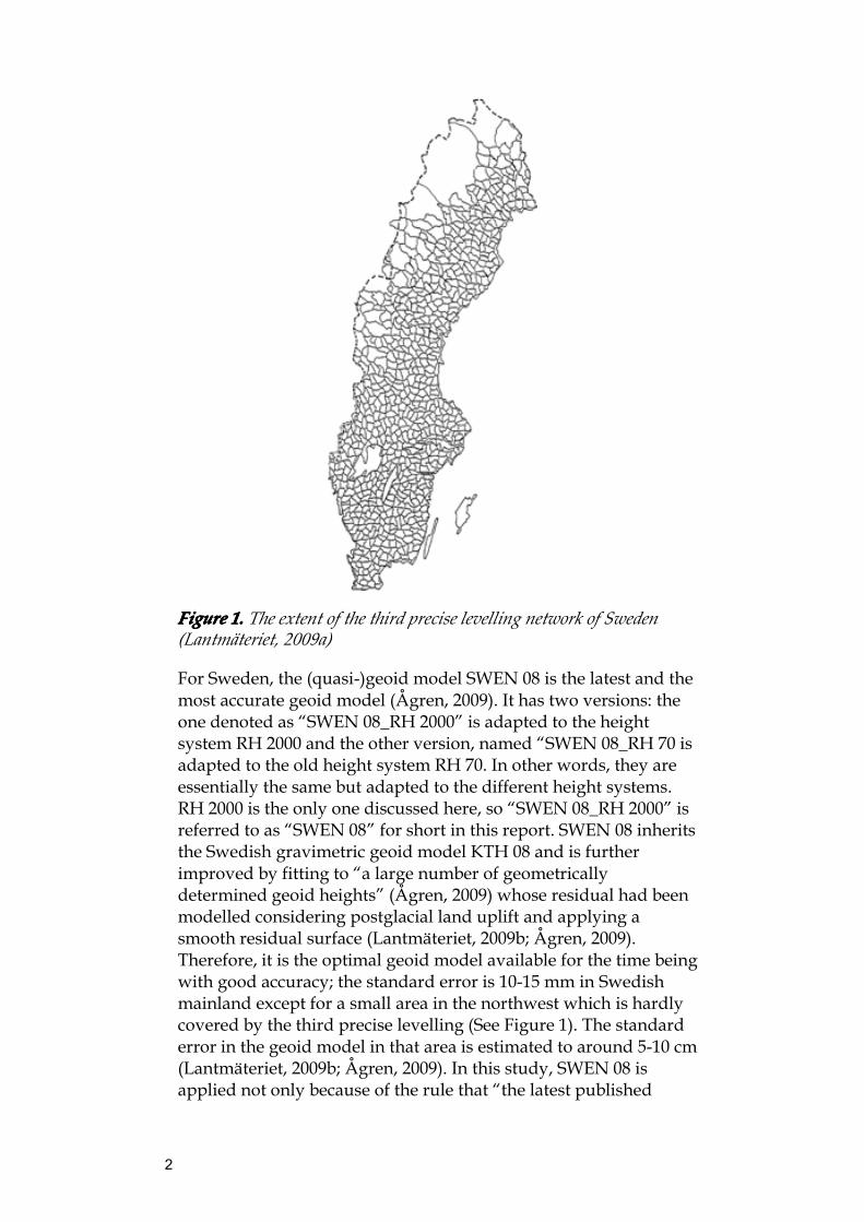
FigureFigureFigureFigure 1.1.1.1. The extent of the third precise levelling network of Sweden(Lantmäteriet, 2009a)

For Sweden, the (quasi-)geoid model SWEN 08 is the latest and themost accurate geoid model (Ågren, 2009). It has two versions: theone denoted as “SWEN 08_RH 2000” is adapted to the heightsystem RH 2000 and the other version, named “SWEN 08_RH 70 isadapted to the old height system RH 70. In other words, they areessentially the same but adapted to the different height systems.RH 2000 is the only one discussed here, so “SWEN 08_RH 2000” isreferred to as “SWEN 08” for short in this report. SWEN 08 inheritsthe Swedish gravimetric geoid model KTH 08 and is furtherimproved by fitting to “a large number of geometricallydetermined geoid heights” (Ågren, 2009) whose residual had beenmodelled considering postglacial land uplift and applying asmooth residual surface (Lantmäteriet, 2009b; Ågren, 2009).Therefore, it is the optimal geoid model available for the time beingwith good accuracy; the standard error is 10-15 mm in Swedishmainland except for a small area in the northwest which is hardlycovered by the third precise levelling (See Figure 1). The standarderror in the geoid model in that area is estimated to around 5-10 cm(Lantmäteriet, 2009b; Ågren, 2009). In this study, SWEN 08 isapplied not only because of the rule that “the latest published

3

version should be used” (Lantmäteriet, 2009b) but also because ofits expected excellent accuracy.

FigureFigureFigureFigure 2.2.2.2. The relation between height above the ellipsoid, normal height,and the (quasi-) geoid

1.11.11.11.1 RRRRevieweviewevieweview onononon formerformerformerformer studiesstudiesstudiesstudiesSince the early days of geodetic applications of GNSS technology,the idea of height determination has been proposed and tested. TheNational Geodetic Survey of the U.S. (NGS) investigated controlsurvey projects with GPS in early 1983, showed that GPS survey"meet a wide range of engineering requirement in vertical control"(Zilkoski, 1990). Up to recently, the difference in reference surfacesbetween GNSS determined ellipsoidal height and physicallymeaningful normal height has been thought as the major problem(eg. Engelis, 1984; Zilkosik, 1990; Featherstone, 2008). The overallmethodology was systematically proposed and tested by Engles(1984, 1985), generally following the Equation (1) to convert theellipsoidal height to normal/orthometric height. Such method iscalled GPS-levelling method (eg. Zilkoski, 1990) or coincide fittingmethod (eg. Hu et al., 2004) in relevant study.

In the “GPS-levelling” method, the geoid height turns to be thecrucial part affecting the accuracy of resulting normal height, sincethe GNSS-determined ellipsoidal height have relatively highaccuracy (Yang et al., 1999; Mårtensson, 2002 and Benahmed Dahoet al., 2006). Regarding the acquirement of the critical geoid height,Yang et al. (1999), Mårtensson (2002) and Featherstone (2008)concluded that in a wide range of applications, provided that thearea is small and/or the surface of geoid is flat, the geometricmethod without gravity correction is thought accurate enough. I.e.,include benchmark with known normal height in the network ofGNSS survey, calculate the geoid height in such positions, and usemethods of interpolation to determine the geoid height of any otherlocation. This method has been proved in many studies, for

4

example, Becker et al. (2002) and Mårtensson (2002). Mårtensson(2002) achieved the relative accuracy of ±10 mm per 10 km usingthe geometric geoid model. However, when the study area is muchlarger and the surface of geoid is not flat, some corrections arethought necessary (Engelis et al., 1985; Yang et al., 1999 andBenahmed Daho et al., 2006). Yang et al. (1999) studied theaccuracy and contributing error sources of a geoid model obtainedwith geometric method in a relatively small area (Hong Kong),proposed that incorporation of a geopotential model and a digitalterrain model can dramatically improve the accuracy. An accuracyof 2 - 3 cm was achieved in Hong Kong.

1.21.21.21.2 AimAimAimAim andandandand objectivesobjectivesobjectivesobjectivesHowever, in the former studies summarized above, the authorsmade their own geoid model mainly because no other accurategeoid model was thought available. It is obvious that the accuracyof the resulting geoid model differs and the result of normalheights is seriously affected with these uncertainties of geoid model.Featherstone (2008) argued “the ellipsoidal height is inherently lessaccurate than horizontal position” due to the various errors inGNSS measurement. The transformation from ellipsoidal height tonormal height worsens the accuracy due to errors of the geoidmodel applied. Therefore, provided that an accurate geoid model,e.g. SWEN 08_RH2000, is available, it will be interesting toinvestigate how the accuracy can be improved comparing to theformer studies.

The objective of this study is to investigate the possibility forconnecting local levelling networks to RH 2000 using GNSStechnology. This is in principle determination of normal heightsusing GNSS, and applying geoid correction using the SWEN 08geoid model. There is still lack of evidence showing how accurateGNSS levelling might be and what kind of application it isqualified to when a good geoid model like SWEN 08 is available.

5

2222 TheTheTheThe GNSSGNSSGNSSGNSS fieldfieldfieldfield experimentexperimentexperimentexperimentThis study is based on a GNSS field experiment performed byLantmäteriet in 2008, which is primarily aimed at establishing a testdata set for evaluating the accuracy of GNSS levelling.

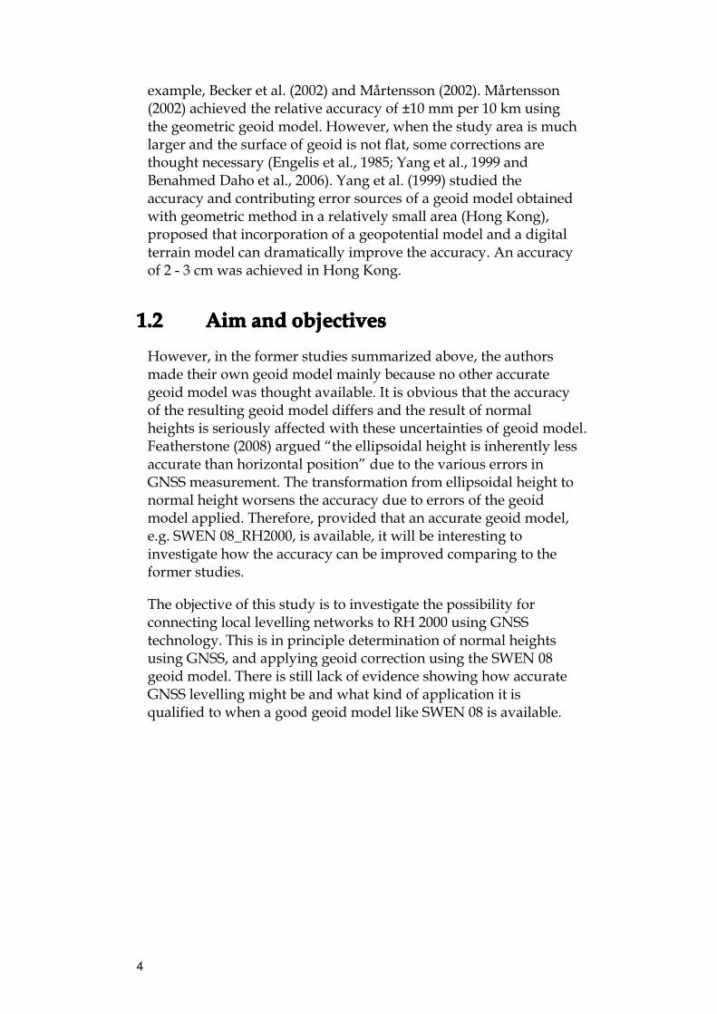
2.12.12.12.1 TheTheTheThe choicechoicechoicechoice ofofofof studystudystudystudy areaareaareaareaAn area in the north-east of Uppsala, Sweden, around a smallvillage named Gåvsta was chosen for the GNSS field experiment,on which this study is based. A local levelling network exists inGåvsta, encircled by a loop that consists of benchmarks of thenational levelling network in RH 2000. See Figure 3 and 4.Previously, the local network has been connected to the nationalheight system by motorized levelling as a densification of thenational network (Becker, 1985). In this GNSS field experiment,some well-distributed benchmarks, in both the national and thelocal network, were chosen to be re-measured with GNSS in orderto establish a test-dataset. Because both GPS-only andGPS/GLONASS receivers are used in the measurement, only theGPS signal has been used in this study. Therefore, the term “GPS”is used on the specific data involved in this study, and the term“GNSS” is used to describe the GNSS data that might be used inthis general methodology. Moreover, in this report, sites 1001, 1002,1003 etc. are referred as sites of ”1000-series” for short. Similarly,sites of “2000-series” refer to sites 2001, 2002, 2003, etc.

FigureFigureFigureFigure 3.3.3.3. Sites measured on February 18 – 20, 2008 : the red dots showsthe benchmarks of national network, the blue ones shows the sites ofdensification and the labelled green ones shows the dots re-measured withGPS (Eriksson, 2009)

6

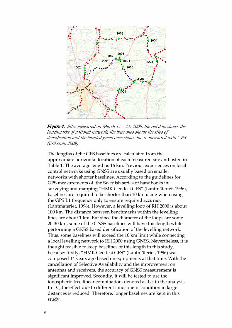
FigureFigureFigureFigure 4.4.4.4. Sites measured on March 17 – 21, 2008: the red dots shows thebenchmarks of national network, the blue ones shows the sites ofdensification and the labelled green ones shows the re-measured with GPS(Eriksson, 2009)

The lengths of the GPS baselines are calculated from theapproximate horizontal location of each measured site and listed inTable 1. The average length is 16 km. Previous experiences on localcontrol networks using GNSS are usually based on smallernetworks with shorter baselines. According to the guidelines forGPS measurements of the Swedish series of handbooks insurveying and mapping “HMK Geodesi GPS” (Lantmäteriet, 1996),baselines are required to be shorter than 10 km using when usingthe GPS L1 frequency only to ensure required accuracy(Lantmäteriet, 1996). However, a levelling loop of RH 2000 is about100 km. The distance between benchmarks within the levellinglines are about 1 km. But since the diameter of the loops are some20-30 km, some of the GNSS baselines will have this length whileperforming a GNSS based densification of the levelling network.Thus, some baselines will exceed the 10 km limit while connectinga local levelling network to RH 2000 using GNSS. Nevertheless, it isthought feasible to keep baselines of this length in this study,because: firstly, “HMK Geodesi GPS” (Lantmäteriet, 1996) wascomposed 14 years ago based on equipments at that time. With thecancellation of Selective Availability and the improvement onantennas and receivers, the accuracy of GNSS measurement issignificant improved. Secondly, it will be tested to use theionospheric-free linear combination, denoted as Lc, in the analysis.In LC, the effect due to different ionospheric condition in largedistances is reduced. Therefore, longer baselines are kept in thisstudy.

7

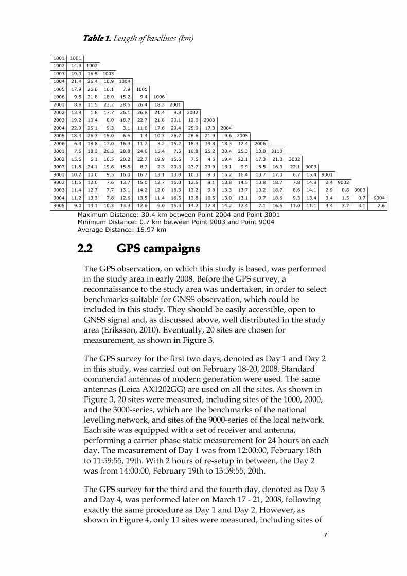
TableTableTableTable 1.1.1.1. Length of baselines (km)

Maximum Distance: 30.4 km between Point 2004 and Point 3001Minimum Distance: 0.7 km between Point 9003 and Point 9004Average Distance: 15.97 km

2.22.22.22.2 GPSGPSGPSGPS campaignscampaignscampaignscampaignsThe GPS observation, on which this study is based, was performedin the study area in early 2008. Before the GPS survey, areconnaissance to the study area was undertaken, in order to selectbenchmarks suitable for GNSS observation, which could beincluded in this study. They should be easily accessible, open toGNSS signal and, as discussed above, well distributed in the studyarea (Eriksson, 2010). Eventually, 20 sites are chosen formeasurement, as shown in Figure 3.

The GPS survey for the first two days, denoted as Day 1 and Day 2in this study, was carried out on February 18-20, 2008. Standardcommercial antennas of modern generation were used. The sameantennas (Leica AX1202GG) are used on all the sites. As shown inFigure 3, 20 sites were measured, including sites of the 1000, 2000,and the 3000-series, which are the benchmarks of the nationallevelling network, and sites of the 9000-series of the local network.Each site was equipped with a set of receiver and antenna,performing a carrier phase static measurement for 24 hours on eachday. The measurement of Day 1 was from 12:00:00, February 18thto 11:59:55, 19th. With 2 hours of re-setup in between, the Day 2was from 14:00:00, February 19th to 13:59:55, 20th.

The GPS survey for the third and the fourth day, denoted as Day 3and Day 4, was performed later on March 17 - 21, 2008, followingexactly the same procedure as Day 1 and Day 2. However, asshown in Figure 4, only 11 sites were measured, including sites of

1001 1001

1002 14.9 1002

1003 19.0 16.5 1003

1004 21.4 25.4 10.9 1004

1005 17.9 26.6 16.1 7.9 1005

1006 9.5 21.8 18.0 15.2 9.4 1006

2001 8.8 11.5 23.2 28.6 26.4 18.3 2001

2002 13.9 1.8 17.7 26.1 26.8 21.4 9.8 2002

2003 19.2 10.4 8.0 18.7 22.7 21.8 20.1 12.0 2003

2004 22.9 25.1 9.3 3.1 11.0 17.6 29.4 25.9 17.3 2004

2005 18.4 26.3 15.0 6.5 1.4 10.3 26.7 26.6 21.9 9.6 2005

2006 6.4 18.8 17.0 16.3 11.7 3.2 15.2 18.3 19.8 18.3 12.4 2006

3001 7.5 18.3 26.3 28.8 24.6 15.4 7.5 16.8 25.2 30.4 25.3 13.0 3110

3002 15.5 6.1 10.5 20.2 22.7 19.9 15.6 7.5 4.6 19.4 22.1 17.3 21.0 3002

3003 11.5 24.1 19.6 15.5 8.7 2.3 20.3 23.7 23.9 18.1 9.9 5.5 16.9 22.1 3003

9001 10.2 10.0 9.5 16.0 16.7 13.1 13.8 10.3 9.3 16.2 16.4 10.7 17.0 6.7 15.4 9001

9002 11.6 12.0 7.6 13.7 15.0 12.7 16.0 12.5 9.1 13.8 14.5 10.8 18.7 7.8 14.8 2.4 9002

9003 11.4 12.7 7.7 13.1 14.2 12.0 16.3 13.2 9.8 13.3 13.7 10.2 18.7 8.6 14.1 2.9 0.8 9003

9004 11.2 13.3 7.8 12.6 13.5 11.4 16.5 13.8 10.5 13.0 13.1 9.7 18.6 9.3 13.4 3.4 1.5 0.7 9004

9005 9.0 14.1 10.3 13.3 12.6 9.0 15.3 14.2 12.8 14.2 12.4 7.1 16.5 11.0 11.1 4.4 3.7 3.1 2.6

8

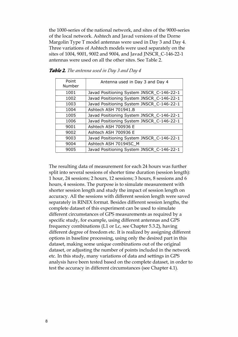
the 1000-series of the national network, and sites of the 9000-seriesof the local network. Ashtech and Javad versions of the DorneMargolin Type T model antennas were used in Day 3 and Day 4.Three variations of Ashtech models were used separately on thesites of 1004, 9001, 9002 and 9004, and Javad JNSCR_C-146-22-1antennas were used on all the other sites. See Table 2.

TableTableTableTable 2222.... The antenna used in Day 3 and Day 4

PointNumber

Antenna used in Day 3 and Day 4

1001 Javad Positioning System JNSCR_C-146-22-11002 Javad Positioning System JNSCR_C-146-22-11003 Javad Positioning System JNSCR_C-146-22-11004 Ashtech ASH 701941.B1005 Javad Positioning System JNSCR_C-146-22-11006 Javad Positioning System JNSCR_C-146-22-19001 Ashtech ASH 700936 E9002 Ashtech ASH 700936 E9003 Javad Positioning System JNSCR_C-146-22-19004 Ashtech ASH 701945C_M9005 Javad Positioning System JNSCR_C-146-22-1

The resulting data of measurement for each 24 hours was furthersplit into several sessions of shorter time duration (session length):1 hour, 24 sessions; 2 hours, 12 sessions; 3 hours, 8 sessions and 6hours, 4 sessions. The purpose is to simulate measurement withshorter session length and study the impact of session length onaccuracy. All the sessions with different session length were savedseparately in RINEX format. Besides different session lengths, thecomplete dataset of this experiment can be used to simulatedifferent circumstances of GPS measurements as required by aspecific study, for example, using different antennas and GPSfrequency combinations (L1 or Lc, see Chapter 5.3.2), havingdifferent degree of freedom etc. It is realized by assigning differentoptions in baseline processing, using only the desired part in thisdataset, making some unique combinations out of the originaldataset, or adjusting the number of points included in the networketc. In this study, many variations of data and settings in GPSanalysis have been tested based on the complete dataset, in order totest the accuracy in different circumstances (see Chapter 4.1).

9

3333 TheTheTheThe mmmmethodethodethodethod ofofofof connectingconnectingconnectingconnecting locallocallocallocallevellinglevellinglevellinglevelling networksnetworksnetworksnetworks totototo RHRHRHRH 2000200020002000

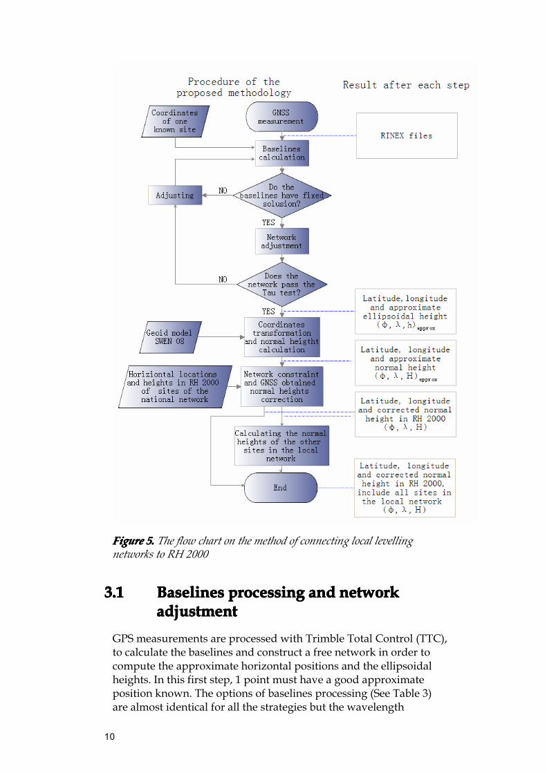
The purpose of this study is to investigate the possibility to connectlocal levelling networks to the national height system RH 2000 inSweden. The methodology applied is generally composed of threeparts. Firstly, compute GPS baselines and perform networkadjustment in a free network. Secondly, transform this free networkinto RH 2000 by using a geoid model and a regional fit to knownpoints in RH 2000. Finally adjust the local levelling network tosome GPS-determined points in RH 2000 from the second step.

In some more detail, the following method is proposed in thisstudy to connect local levelling networks to RH 2000 (see Figure 5):firstly, free network of GPS measurement is calculated andadjusted. The resulting ellipsoidal heights of the benchmarks in thelocal network are transformed into approximate normal heightsusing SWEN08 (Ågren, 2009) as geoid model (Chapter 3.1 and 3.2).Secondly, the resulting network of approximate normal heights isaligned to the known heights in RH 2000 on benchmarks includedin the network by applying a one-dimensional 3-parameter verticaltransformation (an inclined plane). With this transformation, theGPS obtained free network is adjusted to the network of RH 2000and the GPS-obtained approximate normal heights of the localnetwork are corrected. An indicator of quality of this GPS-determined network is also calculated in this step. See Chapter 3.3.Thirdly, the local network is aligned to the GPS-obtained networkby performing a 1-parameter vertical transformation using thebenchmarks in the local network re-measured with GPS ascommon points. With this transformation, the translation valuebetween the local and the national system are calculated. Thereby,the heights in RH 2000 of the other benchmarks in the localnetwork, which are not re-measured with GPS, are computed. SeeChapter 3.4.

The GNSS software Trimble Total Control (Trimble Navigation Ltd.,2002), denoted as “TTC” in this report, have been used in this studyfor baseline calculation and network adjustment. The Gtranstransformation utility (Lantmäteriet 2009c) was used forcoordinates transformation and network fitting, which isessentially a program for coordinates/ heights transformation.

10

FigureFigureFigureFigure 5.5.5.5. The flow chart on the method of connecting local levellingnetworks to RH 2000

3.13.13.13.1 BaselinesBaselinesBaselinesBaselines processingprocessingprocessingprocessing andandandand networknetworknetworknetworkadjustmentadjustmentadjustmentadjustment

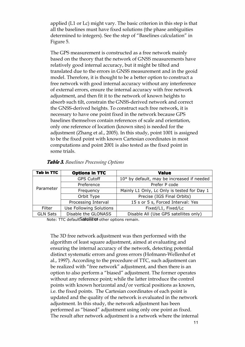
GPS measurements are processed with Trimble Total Control (TTC),to calculate the baselines and construct a free network in order tocompute the approximate horizontal positions and the ellipsoidalheights. In this first step, 1 point must have a good approximateposition known. The options of baselines processing (See Table 3)are almost identical for all the strategies but the wavelength

11

applied (L1 or Lc) might vary. The basic criterion in this step is thatall the baselines must have fixed solutions (the phase ambiguitiesdetermined to integers). See the step of “Baselines calculation” inFigure 5.

The GPS measurement is constructed as a free network mainlybased on the theory that the network of GNSS measurements haverelatively good internal accuracy, but it might be tilted andtranslated due to the errors in GNSS measurement and in the geoidmodel. Therefore, it is thought to be a better option to construct afree network with good internal accuracy without any interferenceof external errors, ensure the internal accuracy with free networkadjustment, and then fit it to the network of known heights toabsorb such tilt, constrain the GNSS-derived network and correctthe GNSS-derived heights. To construct such free network, it isnecessary to have one point fixed in the network because GPSbaselines themselves contain references of scale and orientation,only one reference of location (known sites) is needed for theadjustment (Zhang et al., 2005). In this study, point 1001 is assignedto be the fixed point with known Cartesian coordinates in mostcomputations and point 2001 is also tested as the fixed point insome trials.

TableTableTableTable 3333.... Baselines Processing Options

TabTabTabTab inininin TTCTTCTTCTTC OptionsOptionsOptionsOptions inininin TTCTTCTTCTTC ValueValueValueValue

Parameter

GPS Cutoff 10° by default, may be increased if neededPreference Prefer P codeFrequency Mainly L1 Only, Lc Only is tested for Day 1Orbit Type Precise (IGS Final Orbits)

Processing Interval 15 s or 5 s, Forced Interval: YesFilter Use Following Solutions Fixed/L1, Fixed/Lc

GLN Sats Disable the GLONASSSatellites

Disable All (Use GPS satellites only)Note: TTC default values of other options remain.

The 3D free network adjustment was then performed with thealgorithm of least square adjustment, aimed at evaluating andensuring the internal accuracy of the network, detecting potentialdistinct systematic errors and gross errors (Hofmann-Wellenhof etal., 1997). According to the procedure of TTC, such adjustment canbe realized with “free network” adjustment, and then there is anoption to also perform a “biased” adjustment. The former operateswithout any reference point; while the latter introduce the controlpoints with known horizontal and/or vertical positions as known,i.e. the fixed points. The Cartesian coordinates of each point isupdated and the quality of the network is evaluated in the networkadjustment. In this study, the network adjustment has beenperformed as “biased” adjustment using only one point as fixed.The result after network adjustment is a network where the internal

12

accuracy of the network is determined by the GPS observations,but it is not disturbed by constraints from known points. But itmight be tilted, rotated and translated with respect to the correctpositions because it has not been constrained to more than onepoint. So, the GPS-obtained ellipsoidal heights here are anapproximation that needs to be further corrected.

The resulting (approximate) 3-dimentional SWEREF 99 Cartesiancoordinates of each point are output in the K-file format. Thisformat is essentially a text file with coordinates, developed byLantmäteriet and the specific format used in the coordinatetransformation tool, Gtrans.

Moreover, in Trimble Total Control, an antenna model providesphase centre eccentricity and elevation dependent variationinformation of a calibrated antenna (Trimble Navigation Ltd., 2002).Normally, if the required antenna model is included in TTC, thebaselines processing can be performed without extra preparation.However, in this study, the phase centre variation (PCV) models ofLeica AX1202GG and Javad JNSCR_C146-22-1 antennas are notincluded. Therefore, they must be installed manually beforebaselines processing. In this study, the phase centre variationmodel of Leica AX1202GG and the model of the Javad antenna isavailable on the website of National Geodetic Survey of the U.S.(NGS) 1. The table of elevation- and/or azimuth-dependent antennaphase centre offsets is copied from the website and arranged intospecified format in TTC (see Appendix 1). See Trimble NavigationLtd. (2002).

3.23.23.23.2 CoordinateCoordinateCoordinateCoordinate systemsystemsystemsystem transformationstransformationstransformationstransformations andandandandnormalnormalnormalnormal heightheightheightheight calculationscalculationscalculationscalculations

Before computing normal heights with Equation (1), the resultingSWEREF 99 Cartesian coordinates of all the points must betransformed into SWEREF 99 TM (the national TransverseMercator map projection for Sweden) to fit the coordinates systemapplied by SWEN 08. Then, SWEN 08 is applied as geoid correctionto compute normal heights in RH 2000 of each site (see Figure 5). Inthis study, they are realized with the software of Gtrans. Theresults are horizontal coordinates in SWEREF 99 TM and normalheights in RH 2000. The resulting normal heights are still in a freenetwork. Therefore, they are approximations and need to becorrected by constraining the free network to the known heights ofbench marks in RH 2000.

1 http://www.ngs.noaa.gov/cgi-bin/query_cal_antennas.prl?Model=JNS&Antenna=JNSCR_C146-22-1%20NONE

13

The horizontal coordinates, which required by SWEN 08 to obtaingeoid heights, are also approximations from the free network.Theoretically, potential errors in the horizontal domain might affectthe geoid heights and thereby affecting the resulting normalheights. Nevertheless, it is thought insignificant and can be omittedin this project. The approximate horizontal coordinates is appliedin this study because horizontal locations of the benchmarks of RH2000 themselves are inaccurate. It is the situation in Sweden and inalmost all the other countries that the benchmarks of a heightsystem are not as accurate in horizontal domain as a triangulationpoint. Thus, even if the free network was constrained in horizontaldomain, their latitudes and longitudes are still relatively inaccurate.However, in this study, such errors are thought so insignificant thatcan be ignored in this area of Sweden. Empirically, the maximumabsolute horizontal deviation in static carrier phase GPSmeasurement is expected around 10 m. The elevation abnormity (ζ),i.e., the difference of geoid height, is computed to be 0.03 mm permeter by average between these investigated benchmarks.Therefore, the error will be 0.3 mm even if a significant horizontalerror existed by 10 m in one site. Obviously, theoretically possibleerrors due to the inaccuracy of horizontal location are soinsignificant that it can be ignored in this study. However, it is notproved in this study that the same accuracy can be achieved as atriangulation point in the western and northern part of Swedenwhere the elevation abnormity (ζ) might be steep. Moreover,theoretically possible errors in horizontal position in the GPSmeasurement will also cause tilt in calculated baselines. There islack of investigation in this study on this error. However, the resultshows it is acceptable even if it existed in this study (see Chapter5.1). One possible solution to such problems is to improve thehorizontal accuracy of GPS measurement in horizontal domain,such as connecting the network to permanent GNSS stations (CORS)in the SWEPOS® control network.

3.33.33.33.3 NetworkNetworkNetworkNetwork constraintconstraintconstraintconstraint andandandandGNSSGNSSGNSSGNSS obtainedobtainedobtainedobtainednormalnormalnormalnormal heightsheightsheightsheights correctioncorrectioncorrectioncorrection

After calculating the approximate normal heights, the free networkis ready to be aligned (fitted) to the known heights of benchmarksof RH 2000 included in the network. By doing this, the free networkis adjusted to and made consistent with the network of RH 2000.E.g. the approximate normal heights of the local network in Gåvsta(points of 9000-series) are being corrected. It might need bothvertical shift and rotation about the x- and y-axis to perform suchconstraint. Therefore, a one-dimensional (vertical) 3-parametercoordinate/height transformation (inclined plane transformation)is applied. See Equation (2):

14

Hi= Hi0+C0 - yi0Δα1+xi0Δα2 -Vh (2)

where Hi is normal height in RH 2000, Hi0 is the GNSS determinedapproximate normal height, C0 is the vertical shift between the twoheight systems, Δα1 andΔα2 are rotation angles about the x-axis andthe y-axis, xi0 and yi0 are the (possibly approximate) horizontalcoordinates. Vh is the residual of height for each specific point. Theorigin of this rotation is in the geometrical centre of the network.Therefore, xi0 and yi0 are relative to centre of the network. Thehorizontal coordinates are required with only low accuracy(Hofmann-Wellenhof et al., 1997). The redundant common pointshere is important because they “enable a least square adjustmentand provide necessary check on the computation of the rotation”(Hofmann-Wellenhof et al., 1997). Meanwhile, the standard error ofunit weight (S0) of this transformation is calculated from theresiduals according to the following formula:

2

10

pN

h

f

VS

N=∑

(3)

where S0 is the standard error unit weight of the transformation. Np

is the number of points included. Vh is the residual of height foreach specific point. Nf is the number of redundancies (or degrees offreedom).

Nf= nNp – Nc (4)

where Nc is the number of parameters applied in thetransformation; n is the number of dimension, i.e., n=3 in 3-dimensional Helmert transformation. So, n=1 in this 1-dimensionaltransformation:

Nf= Np – Nc (5)

where Nf, Np and Nc is identical as portrayed above in Equation (3)and (4). The standard error of unit weight of the transformation isan indicator about how the two networks agree, which is anindicator of the quality of GPS height measurement and normalheight calculation with SWEN 08, See Chapter 4.3.1., where all theindicators are explained.

3.43.43.43.4 HeightHeightHeightHeight computationcomputationcomputationcomputation ofofofof thethethethe otherotherotherother sitessitessitessites ininininthethethethe locallocallocallocal networknetworknetworknetwork

Practically, not all the benchmarks in the local network must beobserved with GNSS. The normal heights of the other benchmarks,

15

which were not observed with GNSS, can be subsequentlycomputed by fitting the local network to the GNSS-determinednetwork of normal heights in RH 2000. Based on the formertransformation, the levellings are supposed not to be tilted so andthe local system should not be tilted when aligned to RH 2000. Aone-dimensional (vertical) transformation is therefore applied. Themathematical expression is:

Ht = Hf +C0 - vH (6)

where Ht are the heights after the transformation, i.e. normalheights in RH 2000. Hf are the heights of points in the local systembefore the transformation. C0 is the systematic height shift of thelocal levelling network, and vH is the residuals.

After this step, the normal heights of all the benchmarks in the localnetwork have been resolved and therefore the progress of normalheights determination with GNSS is accomplished. That means thelocal network has been connected to RH 2000.

In this study, all the transformation portrayed above are performedwith Gtrans. Some or all of the benchmarks of RH 2000 re-measured with GPS, e.g. sites of 1000, 2000 and 3000-series, areused as common points. Both the result and the statistics of thetransformations are saved for further analysis. See Chapter 4.

16

4444 EvaluatiEvaluatiEvaluatiEvaluationononon ofofofof thethethethe proposedproposedproposedproposed methodmethodmethodmethodFollowing the same approach as depicted in Chapter 3, many setsof independent computations of normal heights are performedseparately for test. See Chapter 4.1. After obtained the normalheights with GPS, the proposed methodology is evaluated bycomparing the GPS-obtained normal heights with theircorresponding pre-determined (chapter 2.1) normal heights inRH 2000. Statistics will be preformed to compute indicators in eachtest computation. The indicators will be arranged, compared andevaluated (see Chapter 4.3) to conclude proposals for futureapplication (see Chapter 5).

4.14.14.14.1 DesignDesignDesignDesign ofofofof experimentsexperimentsexperimentsexperimentsThe methodology proposed in this study was tested using differentdata and settings. For example, using measurement of differentdays obtained with different antennas, using different sessionduration and GPS frequency combinations (e.g. L1 or Lc),simulating measuring more sites with less GPS receivers, and someother reasonable changes on parameters, as shown in Table 4. Thepurpose of such experiments is to test the accuracy andrepeatability of this approach under different circumstances thatmight exist in applications. By comparing their accuracy, theaffecting elements of the proposed method are identified andanalyzed. The ultimate goal for this study is to be able to proposean optimal combination of observation and analysis strategy forthese kind of survey work. In this study, a full set of data andsettings used in a computation is referred as a "strategy". In otherwords, a “strategy” refers to certain combination of methodologyfor GPS measurements, options in baseline processing, andnetwork adjustment and transformations applied in order to derivenormal heights in RH 2000. Various strategies are designed torealize tests mentioned above, see Table 4. They are organized in 9groups, numbered with Roman numerals in Table 4, and namedaccording to their attributes.

17

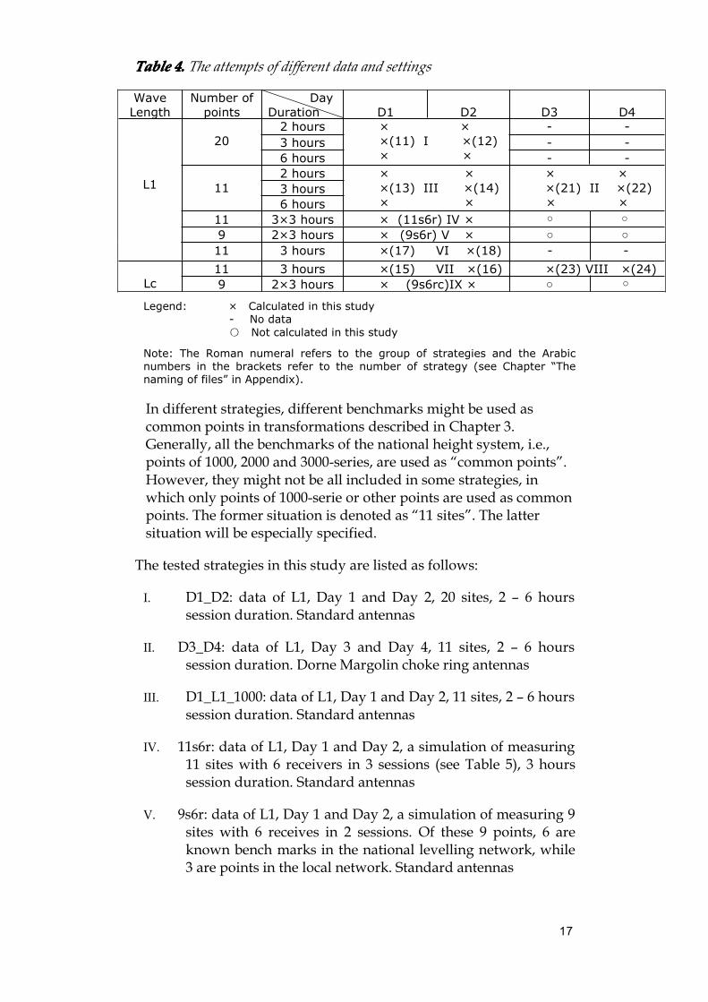
TableTableTableTable 4.4.4.4. The attempts of different data and settings

WaveLength

Number ofpoints

DayDuration D1 D2 D3 D4

L1

202 hours × ×

×(11) I ×(12)× ×

- -3 hours - -6 hours - -

112 hours × ×

×(13) III ×(14)× ×

× ××(21) II ×(22)× ×

3 hours6 hours

11 3×3 hours × (11s6r) IV × ○ ○9 2×3 hours × (9s6r) V × ○ ○11 3 hours ×(17) VI ×(18) - -

Lc11 3 hours ×(15) VII ×(16) ×(23) VIII ×(24)9 2×3 hours × (9s6rc)IX × ○ ○

Legend: × Calculated in this study- No data○ Not calculated in this study

Note: The Roman numeral refers to the group of strategies and the Arabicnumbers in the brackets refer to the number of strategy (see Chapter “Thenaming of files” in Appendix).

In different strategies, different benchmarks might be used ascommon points in transformations described in Chapter 3.Generally, all the benchmarks of the national height system, i.e.,points of 1000, 2000 and 3000-series, are used as “common points”.However, they might not be all included in some strategies, inwhich only points of 1000-serie or other points are used as commonpoints. The former situation is denoted as “11 sites”. The lattersituation will be especially specified.

The tested strategies in this study are listed as follows:

I. D1_D2: data of L1, Day 1 and Day 2, 20 sites, 2 – 6 hourssession duration. Standard antennas

II. D3_D4: data of L1, Day 3 and Day 4, 11 sites, 2 – 6 hourssession duration. Dorne Margolin choke ring antennas

III. D1_L1_1000: data of L1, Day 1 and Day 2, 11 sites, 2 – 6 hourssession duration. Standard antennas

IV. 11s6r: data of L1, Day 1 and Day 2, a simulation of measuring11 sites with 6 receivers in 3 sessions (see Table 5), 3 hourssession duration. Standard antennas

V. 9s6r: data of L1, Day 1 and Day 2, a simulation of measuring 9sites with 6 receives in 2 sessions. Of these 9 points, 6 areknown bench marks in the national levelling network, while3 are points in the local network. Standard antennas

18

VI. D1_D2_L1_2000: data of L1, Day 1 and Day 2, 11 sites in whichsites of 2000-series are used instead of the 1000-series asknown ones, 3 hours session duration. Standard antennas

VII. D1_Lc_1000: data of Lc, Day 1 and Day 2, 11sites, 3 hourssession duration. Standard antennas

VIII. D3_Lc: data of Lc, Day 3 and Day 4, 11sites, 3 hours sessionduration. Dorne Margolin choke ring antennas

IX. 9s6rc: same as 9s6r, but using Lc.

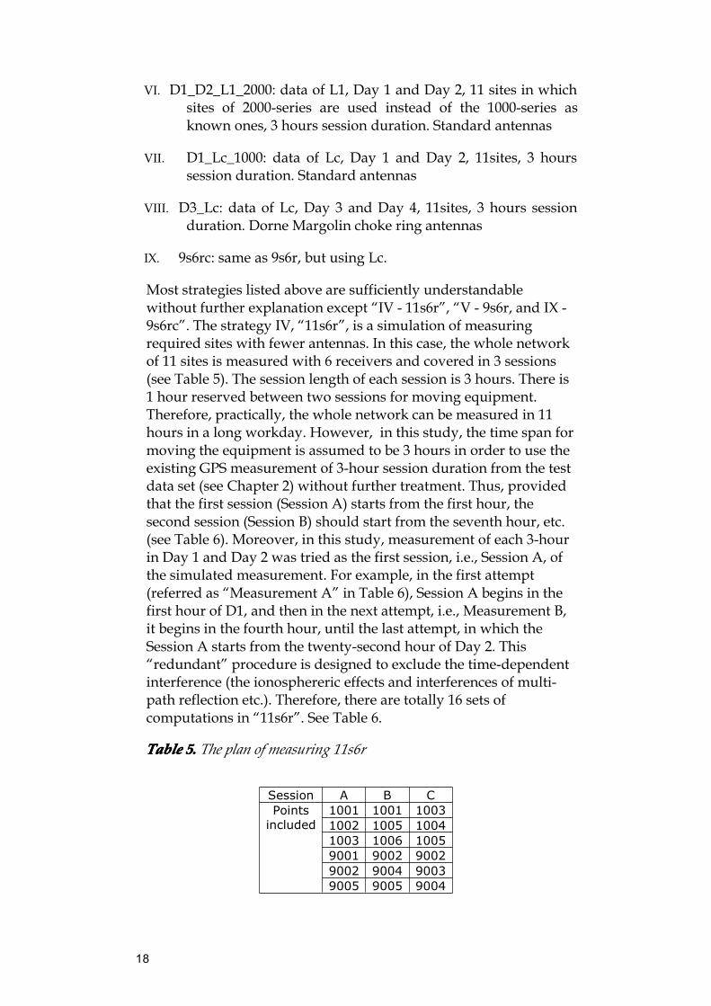
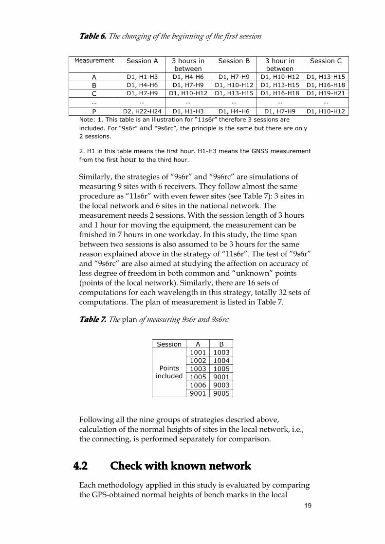
Most strategies listed above are sufficiently understandablewithout further explanation except “IV - 11s6r”, “V - 9s6r, and IX -9s6rc”. The strategy IV, “11s6r”, is a simulation of measuringrequired sites with fewer antennas. In this case, the whole networkof 11 sites is measured with 6 receivers and covered in 3 sessions(see Table 5). The session length of each session is 3 hours. There is1 hour reserved between two sessions for moving equipment.Therefore, practically, the whole network can be measured in 11hours in a long workday. However, in this study, the time span formoving the equipment is assumed to be 3 hours in order to use theexisting GPS measurement of 3-hour session duration from the testdata set (see Chapter 2) without further treatment. Thus, providedthat the first session (Session A) starts from the first hour, thesecond session (Session B) should start from the seventh hour, etc.(see Table 6). Moreover, in this study, measurement of each 3-hourin Day 1 and Day 2 was tried as the first session, i.e., Session A, ofthe simulated measurement. For example, in the first attempt(referred as “Measurement A” in Table 6), Session A begins in thefirst hour of D1, and then in the next attempt, i.e., Measurement B,it begins in the fourth hour, until the last attempt, in which theSession A starts from the twenty-second hour of Day 2. This“redundant” procedure is designed to exclude the time-dependentinterference (the ionosphereric effects and interferences of multi-path reflection etc.). Therefore, there are totally 16 sets ofcomputations in “11s6r”. See Table 6.

TableTableTableTable 5.5.5.5. The plan of measuring 11s6r

Session A B CPoints

included1001 1001 10031002 1005 10041003 1006 10059001 9002 90029002 9004 90039005 9005 9004

19

TableTableTableTable 6.6.6.6. The changing of the beginning of the first session

Measurement Session A 3 hours inbetween

Session B 3 hour inbetween

Session C

A D1, H1-H3 D1, H4-H6 D1, H7-H9 D1, H10-H12 D1, H13-H15

B D1, H4-H6 D1, H7-H9 D1, H10-H12 D1, H13-H15 D1, H16-H18C D1, H7-H9 D1, H10-H12 D1, H13-H15 D1, H16-H18 D1, H19-H21

… … … … … …

P D2, H22-H24 D1, H1-H3 D1, H4-H6 D1, H7-H9 D1, H10-H12Note: 1. This table is an illustration for “11s6r” therefore 3 sessions areincluded. For “9s6r” and “9s6rc”, the principle is the same but there are only2 sessions.

2. H1 in this table means the first hour. H1-H3 means the GNSS measurementfrom the first hour to the third hour.

Similarly, the strategies of “9s6r” and “9s6rc” are simulations ofmeasuring 9 sites with 6 receivers. They follow almost the sameprocedure as “11s6r” with even fewer sites (see Table 7): 3 sites inthe local network and 6 sites in the national network. Themeasurement needs 2 sessions. With the session length of 3 hoursand 1 hour for moving the equipment, the measurement can befinished in 7 hours in one workday. In this study, the time spanbetween two sessions is also assumed to be 3 hours for the samereason explained above in the strategy of “11s6r”. The test of ”9s6r”and “9s6rc” are also aimed at studying the affection on accuracy ofless degree of freedom in both common and “unknown” points(points of the local network). Similarly, there are 16 sets ofcomputations for each wavelength in this strategy, totally 32 sets ofcomputations. The plan of measurement is listed in Table 7.

TableTableTableTable 7777.... The plan of measuring 9s6r and 9s6rc

Session A B

Pointsincluded

1001 10031002 10041003 10051005 90011006 90039001 9005

Following all the nine groups of strategies descried above,calculation of the normal heights of sites in the local network, i.e.,the connecting, is performed separately for comparison.

4.24.24.24.2 CheckCheckCheckCheck withwithwithwith knownknownknownknown networknetworknetworknetworkEach methodology applied in this study is evaluated by comparingthe GPS-obtained normal heights of bench marks in the local

20

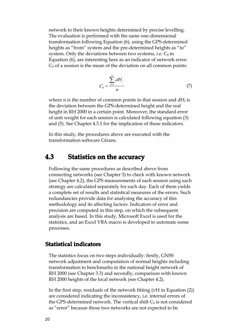
network to their known heights determined by precise levelling.The evaluation is performed with the same one-dimensionaltransformation following Equation (6), using the GPS-determinedheights as “from” system and the pre-determined heights as “to”system. Only the deviations between two systems, i.e. C0 inEquation (6), are interesting here as an indicator of network error.C0 of a session is the mean of the deviation on all common points:

10

n

ii

dHC

n==∑

(7)

where n is the number of common points in that session and dHi isthe deviation between the GPS-determined height and the realheight in RH 2000 in a certain point. Moreover, the standard errorof unit weight for each session is calculated following equation (3)and (5). See Chapter 4.3.1 for the implication of those indicators.

In this study, the procedures above are executed with thetransformation software Gtrans.

4.34.34.34.3 StatisticsStatisticsStatisticsStatistics onononon thethethethe accuracyaccuracyaccuracyaccuracyFollowing the same procedures as described above fromconnecting networks (see Chapter 3) to check with known network(see Chapter 4.2), the GPS measurements of each session using eachstrategy are calculated separately for each day. Each of them yieldsa complete set of results and statistical measures of the errors. Suchredundancies provide data for analysing the accuracy of thismethodology and its affecting factors. Indicators of error andprecision are computed in this step, on which the subsequentanalysis are based. In this study, Microsoft Excel is used for thestatistics, and an Excel VBA macro is developed to automate someprocesses.

StatisticalStatisticalStatisticalStatistical indicatorsindicatorsindicatorsindicators

The statistics focus on two steps individually: firstly, GNSSnetwork adjustment and computation of normal heights includingtransformation to benchmarks in the national height network ofRH 2000 (see Chapter 3.3) and secondly, comparison with knownRH 2000 heights of the local network (see Chapter 4.2).

In the first step, residuals of the network fitting (vH in Equation (2))are considered indicating the inconsistency, i.e. internal errors ofthe GPS-determined network. The vertical shift C0 is not consideredas “error” because those two networks are not expected to be

21

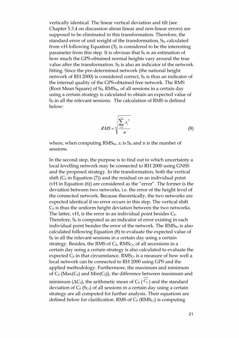
vertically identical. The linear vertical deviation and tilt (seeChapter 5.3.4 on discussion about linear and non-linear errors) aresupposed to be eliminated in this transformation. Therefore, thestandard error of unit weight of the transformation, S0, calculatedfrom vH following Equation (3), is considered to be the interestingparameter from this step. It is obvious that S0 is an estimation ofhow much the GPS-obtained normal heights vary around the truevalue after the transformation. S0 is also an indicator of the networkfitting. Since the pre-determined network (the national heightnetwork of RH 2000) is considered correct, S0 is thus an indicator ofthe internal quality of the GPS-obtained free network. The RMS(Root Mean Square) of S0, RMSS0, of all sessions in a certain dayusing a certain strategy is calculated to obtain an expected value ofS0 in all the relevant sessions. The calculation of RMS is definedbelow:

n

xRMS

n

ii∑

== 1

2

(8)

where, when computing RMSS0, xi is S0i and n is the number ofsessions.

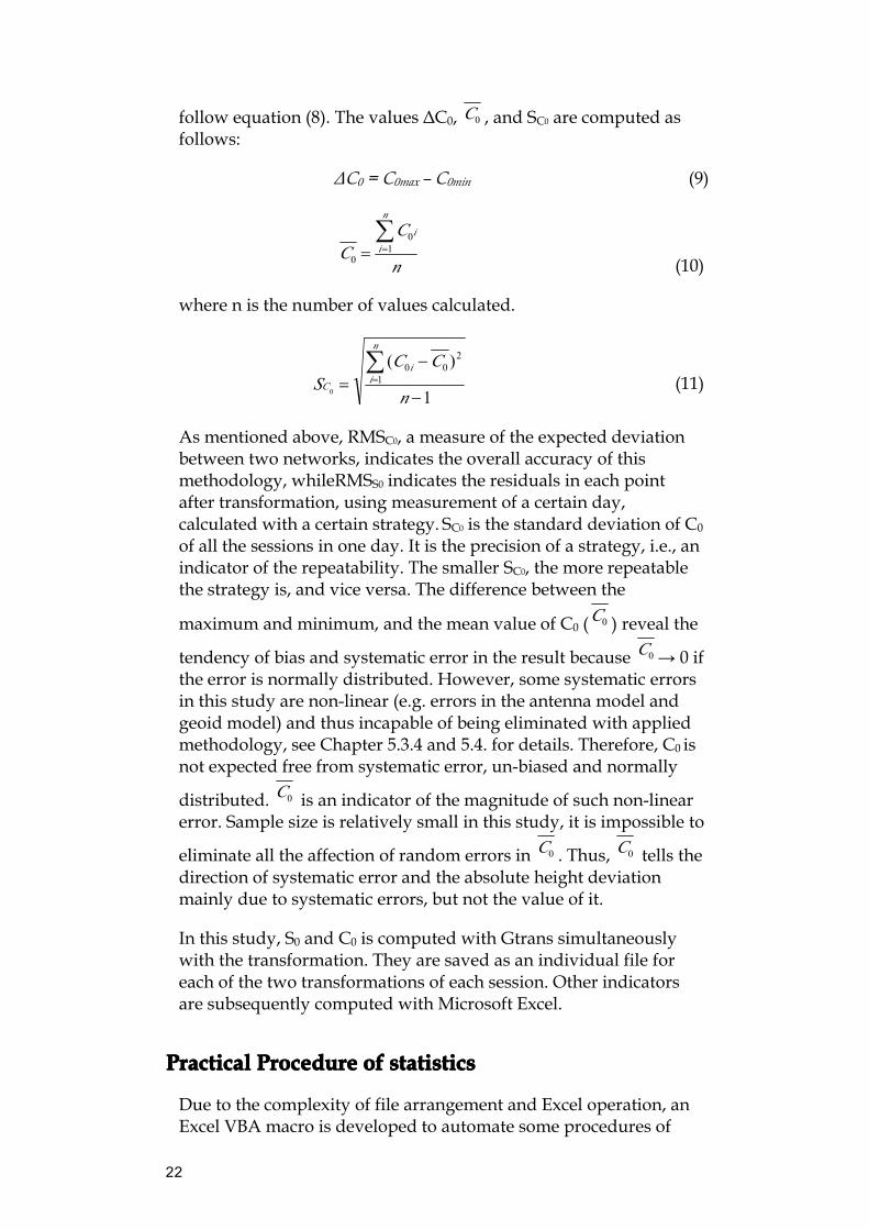
In the second step, the purpose is to find out to which uncertainty alocal levelling network may be connected to RH 2000 using GNSSand the proposed strategy. In the transformation, both the verticalshift (C0 in Equation (7)) and the residual on an individual point(vH in Equation (6)) are considered as the “error”. The former is thedeviation between two networks, i.e. the error of the height level ofthe connected network. Because theoretically, the two networks areexpected identical if no error occurs in this step. The vertical shiftC0 is thus the uniform height deviation between the two networks.The latter, vH, is the error in an individual point besides C0.Therefore, S0 is computed as an indicator of error existing in eachindividual point besides the error of the network. The RMSSo is alsocalculated following Equation (8) to evaluate the expected value ofS0 in all the relevant sessions in a certain day using a certainstrategy. Besides, the RMS of C0, RMSC0, of all secessions in acertain day using a certain strategy is also calculated to evaluate theexpected C0 in that circumstance. RMSC0 is a measure of how well alocal network can be connected to RH 2000 using GPS and theapplied methodology. Furthermore, the maximum and minimumof C0 (Max(C0) and Min(C0)), the difference between maximum andminimum (ΔC0), the arithmetic mean of C0 ( 0C ) and the standarddeviation of C0 (SC0) of all sessions in a certain day using a certainstrategy are all computed for further analysis. Their equations aredefined below for clarification. RMS of C0 (RMSC0) is computing

22

follow equation (8). The values ΔC0, 0C , and SC0 are computed asfollows:

ΔC0 = C0max – C0min (9)

n

CC

n

ii∑

== 10

0 (10)

where n is the number of values calculated.

1

)(1

200

0 −

−=∑=

n

CCS

n

ii

C (11)

As mentioned above, RMSC0, a measure of the expected deviationbetween two networks, indicates the overall accuracy of thismethodology, whileRMSS0 indicates the residuals in each pointafter transformation, using measurement of a certain day,calculated with a certain strategy. SC0 is the standard deviation of C0

of all the sessions in one day. It is the precision of a strategy, i.e., anindicator of the repeatability. The smaller SC0, the more repeatablethe strategy is, and vice versa. The difference between the

maximum and minimum, and the mean value of C0 ( 0C ) reveal the

tendency of bias and systematic error in the result because 0C → 0 ifthe error is normally distributed. However, some systematic errorsin this study are non-linear (e.g. errors in the antenna model andgeoid model) and thus incapable of being eliminated with appliedmethodology, see Chapter 5.3.4 and 5.4. for details. Therefore, C0 isnot expected free from systematic error, un-biased and normally

distributed. 0C is an indicator of the magnitude of such non-linearerror. Sample size is relatively small in this study, it is impossible to

eliminate all the affection of random errors in 0C . Thus, 0C tells thedirection of systematic error and the absolute height deviationmainly due to systematic errors, but not the value of it.

In this study, S0 and C0 is computed with Gtrans simultaneouslywith the transformation. They are saved as an individual file foreach of the two transformations of each session. Other indicatorsare subsequently computed with Microsoft Excel.

PracticalPracticalPracticalPractical ProcedureProcedureProcedureProcedure ofofofof statisticsstatisticsstatisticsstatistics

Due to the complexity of file arrangement and Excel operation, anExcel VBA macro is developed to automate some procedures of

23

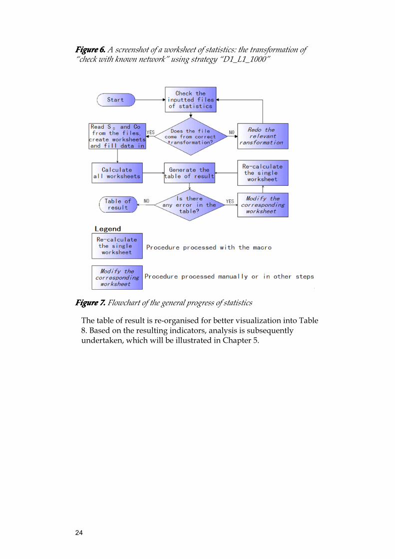
statistics (see Appendix 2). It is composed of five relativelyindependent subroutines (See Figure. 6), including:

1. check the input files of statistics: read input files, creatingcorresponding worksheets and fill in data

2. calculate indicators of all the worksheets

3. calculate a single worksheet

4. generate the table of result.

With the macro, the input files of statistics are firstly automaticallychecked to see if it is the desired one, i.e., if it was generated withthe correct transformation. If any trace of error found, the relevanttransformation must be re-computed in Gtrans. With correct inputfiles of statistics, S0 in the first transformation, as well as S0 and C0

in the second transformation are loaded. They are arranged withthe step of transformation, day, session duration and strategyapplied and subsequently filled into their correspondingworksheets. One worksheet is created for each step oftransformation of a strategy, i.e., for each strategy, two worksheets,separate for “network constraint” and for “check with knownnetwork” are created. Then, statistical indicators are calculated ineach worksheet and eventually organized into the table of result(Table 8). Figure 6 shows the general structure of such Excelworksheet for statistics. If any error was found in a singleworksheet, the problem must be solved and that single worksheetcan be calculated individually after modifications and the table ofresult can be generated again. See Figure 7.

24

FigureFigureFigureFigure 6666.... A screenshot of a worksheet of statistics: the transformation of“check with known network” using strategy “D1_L1_1000”

FigureFigureFigureFigure 7777.... Flowchart of the general progress of statistics

The table of result is re-organised for better visualization into Table8. Based on the resulting indicators, analysis is subsequentlyundertaken, which will be illustrated in Chapter 5.

25

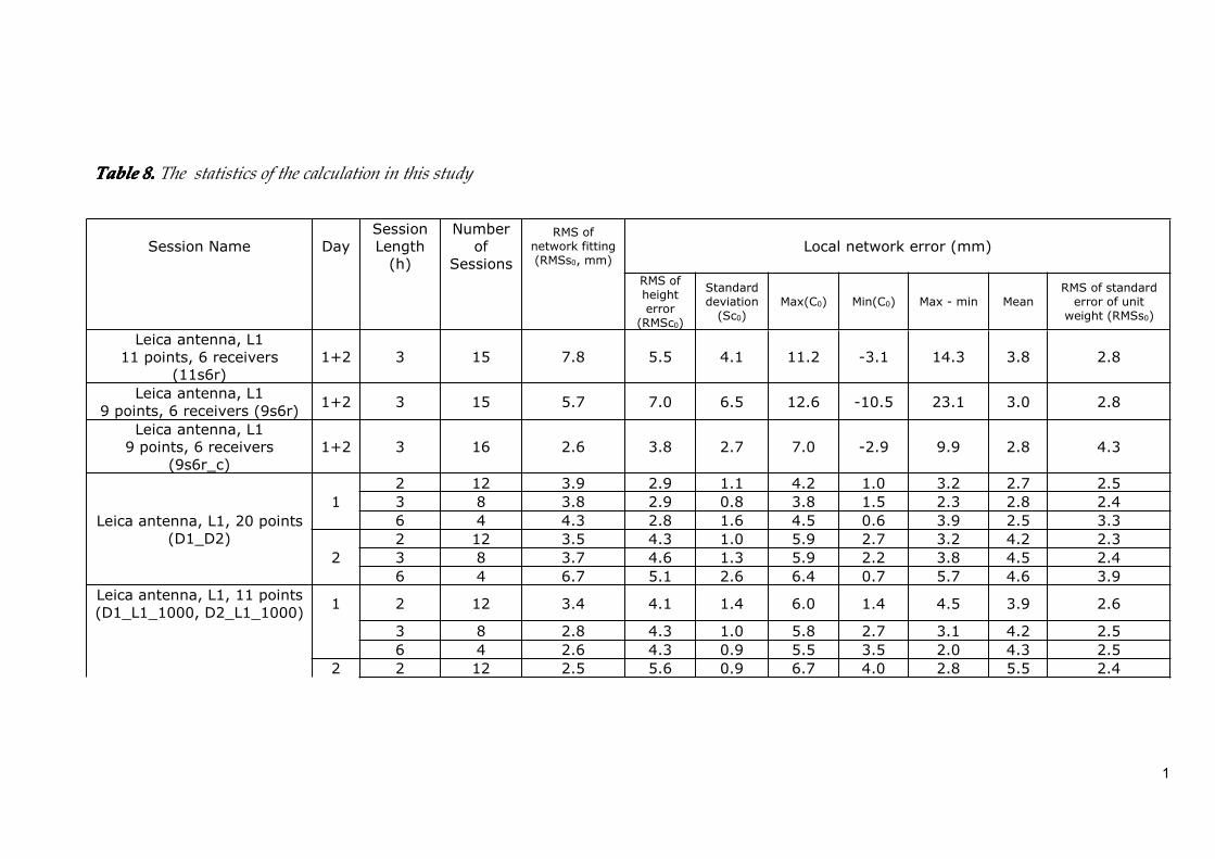
5555 ResultResultResultResult andandandand analysisanalysisanalysisanalysisThe GPS obtained normal heights in RH 2000 and the statisticalindicators constitute the result of this study. The latter reveals thefeasibility and accuracy of this methodology and is therefore ofoutmost interest. The results are summarized in Table 8.

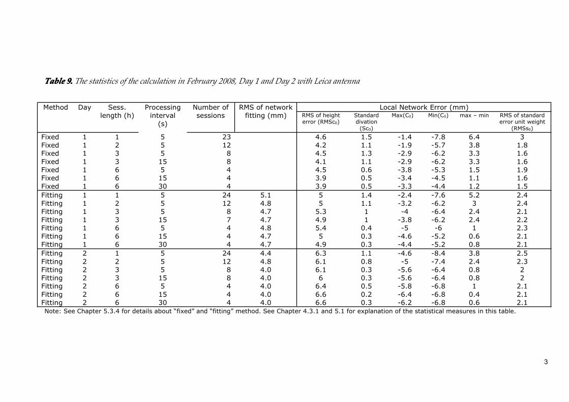
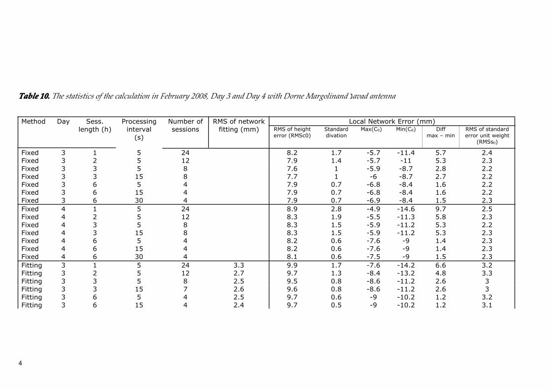
In 2008, Lantmäteriet performed a comparable analysis based onthe same GPS measurement, using different software and settings.GeoGenius from TerraSAT GmbH was applied for GPSmeasurement processing, using broadcast orbit. Many processingtime interval were tried, including 5 seconds, 15 seconds and 30seconds while processing interval of 15-second is uniformlyapplied in this study, see Table 3. The former geoid modelSWEN05_RH2000 was used in the analysis from 2008. Moreover,two different methods of network fitting were tested in the formercalculation, denoted as “fitting” and “fixed”. The former is thesame method applied in this study (see Chapter 3.1 and 3.3), i.e.,free network adjustment with one point fixed and then constrainedto the known network by 1-dimentional 3-parametertransformation. The latter is to assign the correct heights to all theincluded benchmarks of the national network during networkadjustment, rather than performing a free network adjustment andthen a transformation. Therefore, the GPS-determined network isdirectly constraint (fixed) to the national network with networkadjustment. See Chapter 5.3.4. The results of this former analysis ofthe same observation campaign are listed in Table 9 and 10. Theyare discussed together in this study in order to analyze the factorseffecting the accuracy with more samples.

1

TableTableTableTable 8888.... The statistics of the calculation in this study

Session Name DaySessionLength

(h)

Numberof

Sessions

RMS ofnetwork fitting(RMSs0, mm)

Local network error (mm)

RMS ofheighterror

(RMSc0)

Standarddeviation

(Sc0)Max(C0) Min(C0) Max - min Mean

RMS of standarderror of unit

weight (RMSs0)

Leica antenna, L111 points, 6 receivers

(11s6r)1+2 3 15 7.8 5.5 4.1 11.2 -3.1 14.3 3.8 2.8

Leica antenna, L19 points, 6 receivers (9s6r)

1+2 3 15 5.7 7.0 6.5 12.6 -10.5 23.1 3.0 2.8

Leica antenna, L19 points, 6 receivers

(9s6r_c)1+2 3 16 2.6 3.8 2.7 7.0 -2.9 9.9 2.8 4.3

Leica antenna, L1, 20 points(D1_D2)

12 12 3.9 2.9 1.1 4.2 1.0 3.2 2.7 2.53 8 3.8 2.9 0.8 3.8 1.5 2.3 2.8 2.46 4 4.3 2.8 1.6 4.5 0.6 3.9 2.5 3.3

22 12 3.5 4.3 1.0 5.9 2.7 3.2 4.2 2.33 8 3.7 4.6 1.3 5.9 2.2 3.8 4.5 2.46 4 6.7 5.1 2.6 6.4 0.7 5.7 4.6 3.9

Leica antenna, L1, 11 points(D1_L1_1000, D2_L1_1000)

1 2 12 3.4 4.1 1.4 6.0 1.4 4.5 3.9 2.6

3 8 2.8 4.3 1.0 5.8 2.7 3.1 4.2 2.56 4 2.6 4.3 0.9 5.5 3.5 2.0 4.3 2.5

2 2 12 2.5 5.6 0.9 6.7 4.0 2.8 5.5 2.4

2

3 8 1.9 5.5 0.8 6.1 4.1 2.1 5.5 2.46 4 1.9 5.4 0.7 5.9 4.4 1.5 5.3 2.3

Leica antenna, Lc, 11 points(D1_Lc_1000, D2_Lc_1000)

1 3 7 2.6 4.1 1.4 5.5 1.9 3.6 3.9 3.1

2 3 8 2.2 5.2 0.9 6.7 3.9 2.8 5.1 3.9Leica antenna, L1, 11

points, points of 2000-series are used as known

(D1_D2_L1_2000)

1 3 8 5.8 2.7 1.3 4.1 0.0 4.1 2.4 2.4

2 3 7 5.8 4.7 1.5 7.0 2.4 4.5 4.5 2.3

DM antenna, L1, 11 points(D3_D4)

32 11 5.0 8.8 1.6 12.7 7.0 5.8 8.7 4.63 8 4.7 8.6 1.0 10.1 7.4 2.7 8.5 4.56 4 4.3 6.9 1.5 8.2 4.9 3.4 6.8 4.7

42 12 3.4 9.0 1.9 10.5 3.6 6.9 8.8 4.33 8 3.2 9.0 1.8 11.1 5.2 5.9 8.8 4.26 4 3.9 6.4 2.4 9.3 3.8 5.5 6.0 4.6

DM antenna, Lc, 11 points(D3_Lc, D4_Lc)

3 3 8 4.3 7.8 0.9 9.3 6.2 3.1 7.8 4.44 3 8 3.6 8.2 1.2 10.4 7.1 3.2 8.1 4.5

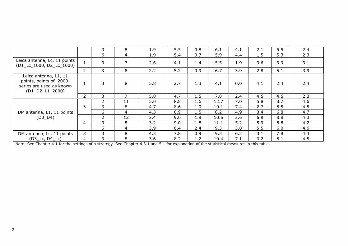
Note: See Chapter 4.1 for the settings of a strategy. See Chapter 4.3.1 and 5.1 for explanation of the statistical measures in this table.

3

TableTableTableTable 9999.... The statistics of the calculation in February 2008, Day 1 and Day 2 with Leica antenna

Method Day Sess.length (h)

Processinginterval

(s)

Number ofsessions

RMS of networkfitting (mm)

Local Network Error (mm)RMS of heighterror (RMSc0)

Standarddivation

(Sc0)

Max(C0) Min(C0) max – min RMS of standarderror unit weight

(RMSs0)

Fixed 1 1 5 23 4.6 1.5 -1.4 -7.8 6.4 3Fixed 1 2 5 12 4.2 1.1 -1.9 -5.7 3.8 1.8Fixed 1 3 5 8 4.5 1.3 -2.9 -6.2 3.3 1.6Fixed 1 3 15 8 4.1 1.1 -2.9 -6.2 3.3 1.6Fixed 1 6 5 4 4.5 0.6 -3.8 -5.3 1.5 1.9Fixed 1 6 15 4 3.9 0.5 -3.4 -4.5 1.1 1.6Fixed 1 6 30 4 3.9 0.5 -3.3 -4.4 1.2 1.5Fitting 1 1 5 24 5.1 5 1.4 -2.4 -7.6 5.2 2.4Fitting 1 2 5 12 4.8 5 1.1 -3.2 -6.2 3 2.4Fitting 1 3 5 8 4.7 5.3 1 -4 -6.4 2.4 2.1Fitting 1 3 15 7 4.7 4.9 1 -3.8 -6.2 2.4 2.2Fitting 1 6 5 4 4.8 5.4 0.4 -5 -6 1 2.3Fitting 1 6 15 4 4.7 5 0.3 -4.6 -5.2 0.6 2.1Fitting 1 6 30 4 4.7 4.9 0.3 -4.4 -5.2 0.8 2.1Fitting 2 1 5 24 4.4 6.3 1.1 -4.6 -8.4 3.8 2.5Fitting 2 2 5 12 4.8 6.1 0.8 -5 -7.4 2.4 2.3Fitting 2 3 5 8 4.0 6.1 0.3 -5.6 -6.4 0.8 2Fitting 2 3 15 8 4.0 6 0.3 -5.6 -6.4 0.8 2Fitting 2 6 5 4 4.0 6.4 0.5 -5.8 -6.8 1 2.1Fitting 2 6 15 4 4.0 6.6 0.2 -6.4 -6.8 0.4 2.1Fitting 2 6 30 4 4.0 6.6 0.3 -6.2 -6.8 0.6 2.1Note: See Chapter 5.3.4 for details about “fixed” and “fitting” method. See Chapter 4.3.1 and 5.1 for explanation of the statistical measures in this table.

4

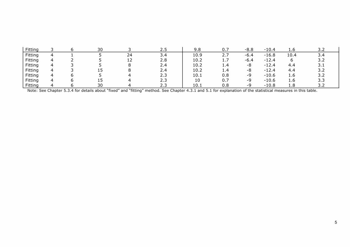
TableTableTableTable 10101010.... The statistics of the calculation in February 2008, Day 3 and Day 4 with Dorne Margolinand Javad antenna

Method Day Sess.length (h)

Processinginterval

(s)

Number ofsessions

RMS of networkfitting (mm)

Local Network Error (mm)RMS of heighterror (RMSc0)

Standarddivation

Max(C0) Min(C0) Diffmax – min

RMS of standarderror unit weight

(RMSs0)

Fixed 3 1 5 24 8.2 1.7 -5.7 -11.4 5.7 2.4Fixed 3 2 5 12 7.9 1.4 -5.7 -11 5.3 2.3Fixed 3 3 5 8 7.6 1 -5.9 -8.7 2.8 2.2Fixed 3 3 15 8 7.7 1 -6 -8.7 2.7 2.2Fixed 3 6 5 4 7.9 0.7 -6.8 -8.4 1.6 2.2Fixed 3 6 15 4 7.9 0.7 -6.8 -8.4 1.6 2.2Fixed 3 6 30 4 7.9 0.7 -6.9 -8.4 1.5 2.3Fixed 4 1 5 24 8.9 2.8 -4.9 -14.6 9.7 2.5Fixed 4 2 5 12 8.3 1.9 -5.5 -11.3 5.8 2.3Fixed 4 3 5 8 8.3 1.5 -5.9 -11.2 5.3 2.2Fixed 4 3 15 8 8.3 1.5 -5.9 -11.2 5.3 2.3Fixed 4 6 5 4 8.2 0.6 -7.6 -9 1.4 2.3Fixed 4 6 15 4 8.2 0.6 -7.6 -9 1.4 2.3Fixed 4 6 30 4 8.1 0.6 -7.5 -9 1.5 2.3Fitting 3 1 5 24 3.3 9.9 1.7 -7.6 -14.2 6.6 3.2Fitting 3 2 5 12 2.7 9.7 1.3 -8.4 -13.2 4.8 3.3Fitting 3 3 5 8 2.5 9.5 0.8 -8.6 -11.2 2.6 3Fitting 3 3 15 7 2.6 9.6 0.8 -8.6 -11.2 2.6 3Fitting 3 6 5 4 2.5 9.7 0.6 -9 -10.2 1.2 3.2Fitting 3 6 15 4 2.4 9.7 0.5 -9 -10.2 1.2 3.1

5

Fitting 3 6 30 3 2.5 9.8 0.7 -8.8 -10.4 1.6 3.2Fitting 4 1 5 24 3.4 10.9 2.7 -6.4 -16.8 10.4 3.4Fitting 4 2 5 12 2.8 10.2 1.7 -6.4 -12.4 6 3.2Fitting 4 3 5 8 2.4 10.2 1.4 -8 -12.4 4.4 3.1Fitting 4 3 15 8 2.4 10.2 1.4 -8 -12.4 4.4 3.2Fitting 4 6 5 4 2.3 10.1 0.8 -9 -10.6 1.6 3.2Fitting 4 6 15 4 2.3 10 0.7 -9 -10.6 1.6 3.3Fitting 4 6 30 4 2.3 10.1 0.8 -9 -10.8 1.8 3.2Note: See Chapter 5.3.4 for details about “fixed” and “fitting” method. See Chapter 4.3.1 and 5.1 for explanation of the statistical measures in this table.

27

5.15.15.15.1 SomeSomeSomeSome explanationexplanationexplanationexplanation onononon thethethethe tablestablestablestables ofofofof resultresultresultresultThe table of statistics of this study, Table 8, can be understood asthree components. Firstly, the first column to the fourth columnillustrates the data used and strategy applied in that trial ofcomputation. Secondly, the fifth column, RMS of network fitting ,lists RMS of standard error of unit weight ( osRMS ) in the firsttransformation, i.e., free network constraint. Thirdly, the sixthcolumn to the last column is indicators from the secondtransformation, i.e., comparing with the pre-determined network.

The tables of statistics of the former analysis, Table 9 and 10, havevery similar structure. As mentioned before, there were twomethods of network fitting tried in that study, they aredistinguished with “fixed” and “fitting” in the first column.

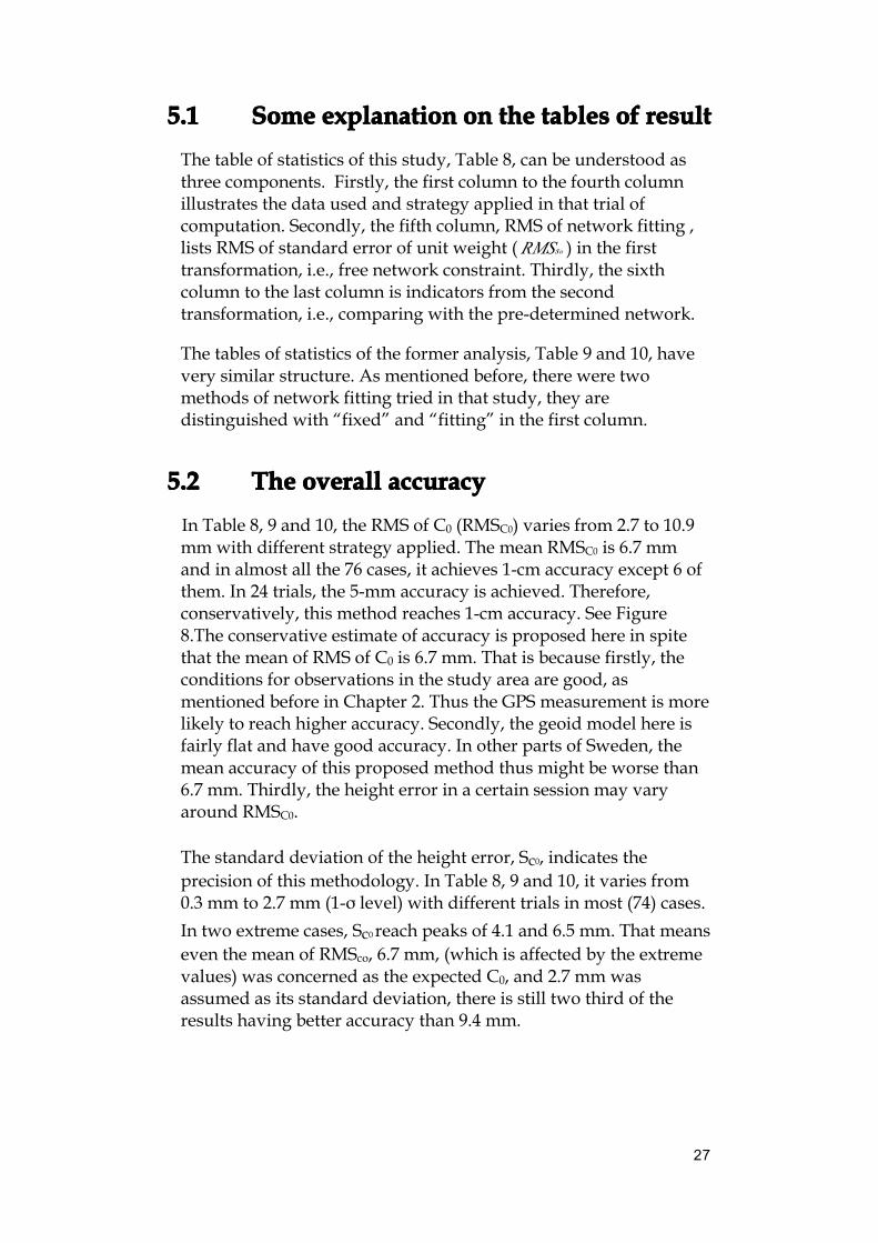
5.25.25.25.2 TheTheTheThe overalloveralloveralloverall accuracyaccuracyaccuracyaccuracyIn Table 8, 9 and 10, the RMS of C0 (RMSC0) varies from 2.7 to 10.9mm with different strategy applied. The mean RMSC0 is 6.7 mmand in almost all the 76 cases, it achieves 1-cm accuracy except 6 ofthem. In 24 trials, the 5-mm accuracy is achieved. Therefore,conservatively, this method reaches 1-cm accuracy. See Figure8.The conservative estimate of accuracy is proposed here in spitethat the mean of RMS of C0 is 6.7 mm. That is because firstly, theconditions for observations in the study area are good, asmentioned before in Chapter 2. Thus the GPS measurement is morelikely to reach higher accuracy. Secondly, the geoid model here isfairly flat and have good accuracy. In other parts of Sweden, themean accuracy of this proposed method thus might be worse than6.7 mm. Thirdly, the height error in a certain session may varyaround RMSC0.

The standard deviation of the height error, Sc0, indicates theprecision of this methodology. In Table 8, 9 and 10, it varies from0.3 mm to 2.7 mm (1-σ level) with different trials in most (74) cases.In two extreme cases, Sc0 reach peaks of 4.1 and 6.5 mm. That meanseven the mean of RMSco, 6.7 mm, (which is affected by the extremevalues) was concerned as the expected C0, and 2.7 mm wasassumed as its standard deviation, there is still two third of theresults having better accuracy than 9.4 mm.

28

FigureFigureFigureFigure 8.8.8.8. RMS and standard deviation of height errors

To achieve this level of accuracy, the RMS of network fitting in thefirst transformation (RMSso) varies from 1.9 mm to 7.8 mm, i.e., thefinal accuracy might not been achieved if the GPS measurement isworse. Moreover, the RMSso in the second transformation is from1.6 mm to 4.7 mm besides C0.

In conclusion, this result reveals that with static GPS observation,with commercial GPS software and SWEN 08 as geoid model, it isfeasible to achieve 1 cm accuracy (1σ) in height determination inmajor part of Sweden.

5.35.35.35.3 AccuracyAccuracyAccuracyAccuracy withwithwithwith regardsregardsregardsregards totototo differentdifferentdifferentdifferentfactorsfactorsfactorsfactors

This chapter focus on the impact of a single factor upon the quality,especially the accuracy and repeatability, of this method. Differentoptions of a parameter are compared while other parameters arekept fixed, to ensure that the result is affected only by the analyzedfactor.

SessionSessionSessionSession durationdurationdurationduration

The impact of session duration is evaluated by comparingstatistical indicators computed using 1-hour, 2-hour 3-hour and 6-hour observation. Only comparable strategies are comparedtogether to ensure that all the other parameters except sessionduration are identical. The comparison is performed by using anindicator of shorter observation time minus the same indicator oflonger observation time: the RMSC0or SC0 of 1-hour observationminus the same indicator of 2-hour observation, etc. The

29

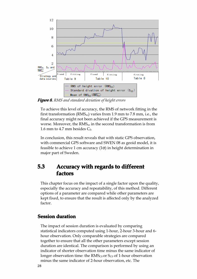
differences shows the tendency of change. In Table 11, thecomparison using statistics of the former study is given. Table 12 isthe same comparison using statistics of this study. For a bettervisualization, Figure 9 and Figure 10 is plotted out of Table 11 andTable 12 separately.

TableTableTableTable 11111111.... The impact of observation time on accuracy (study in 2008),Unit: mm

Method ΔRMSCo

1h-2hΔRMSCo

2h-3hΔRMSCo

3h-6hΔSCo

1h-2hΔSCo

2h-3hΔSCo

3h-6hFixed Day 1 0.4 -0.3 0 0.4 -0.2 0.7Fitting day 1 0 -0.3 -0.1 0.3 0.1 0.6Fitting day 2 0.2 0 -0.3 0.3 0.5 -0.2fixed Day 3 0.3 0.3 -0.3 0.3 0.4 0.3Fixed Day 4 0.6 0 0.1 0.9 0.4 0.9fitting Day 3 0.2 0.2 -0.2 0.4 0.5 0.2fitting Day 4 0.7 0 0.1 1 0.3 0.6

Mean 0.3 -0.01 -0.1 0.5 0.3 0.4

-0.4

-0.2

0

0.2

0.4

0.6

0.8

1

1h-2h 2h-3h 3h-6h 1h-2h 2h-3h 3h-6h

ΔRMSCo ΔRMSCo ΔRMSCo ΔSCo ΔSCo ΔSCo

Fixed Day 1

Fitting day 1

Fitting day 2

fixed Day 3

Fixed Day 4

fitting Day 3

fitting Day 4

FigureFigureFigureFigure 9.9.9.9. The effect of observation time to accuracy (calculation of 2008),Unit mm

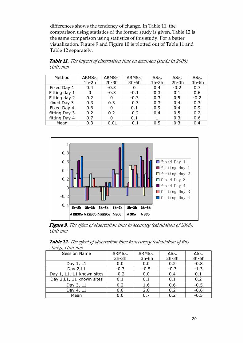
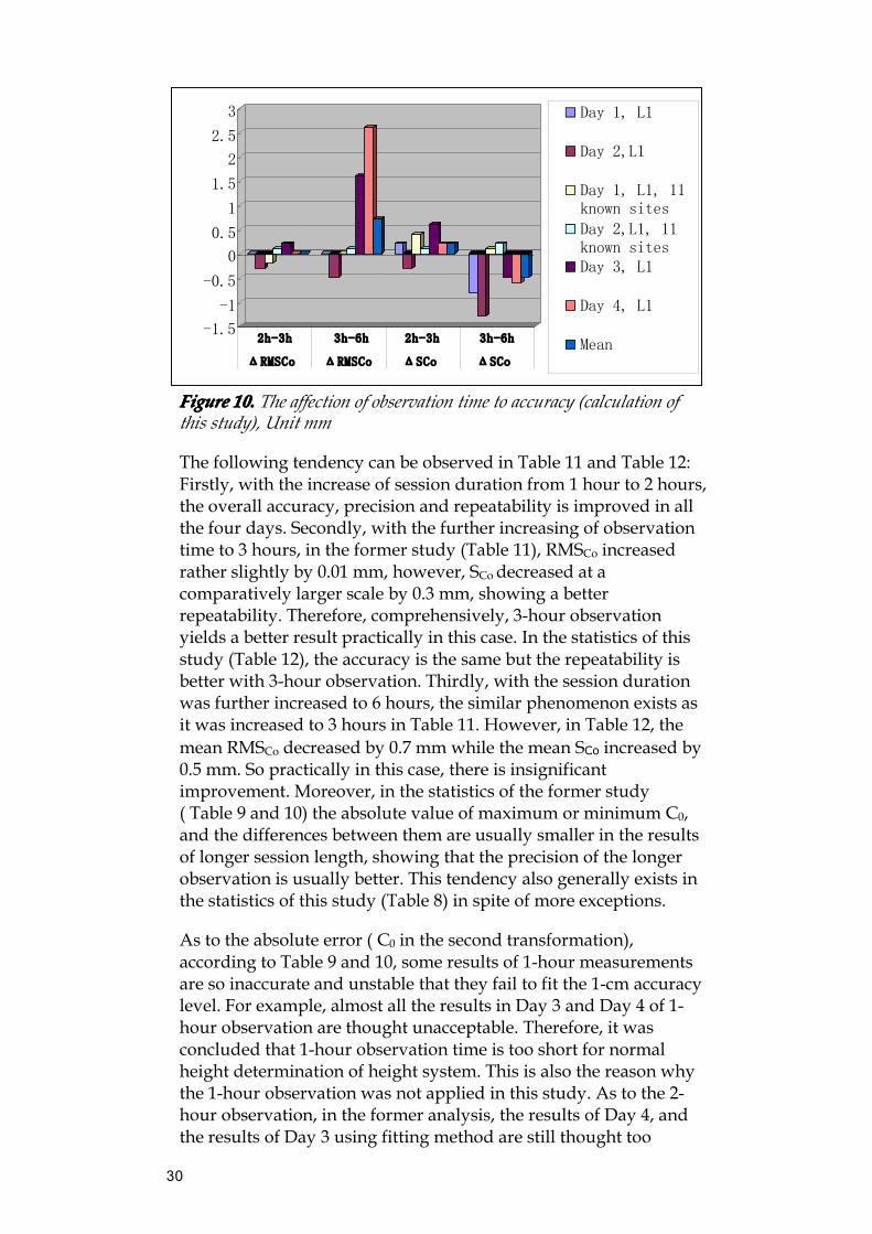
TableTableTableTable 12121212.... The effect of observation time to accuracy (calculation of thisstudy), Unit mm

Session Name ΔRMSCo

2h-3hΔRMSCo

3h-6hΔSCo

2h-3hΔSCo

3h-6hDay 1, L1 0.0 0.0 0.2 -0.8Day 2,L1 -0.3 -0.5 -0.3 -1.3

Day 1, L1, 11 known sites -0.2 0.0 0.4 0.1Day 2,L1, 11 known sites 0.1 0.1 0.1 0.2

Day 3, L1 0.2 1.6 0.6 -0.5Day 4, L1 0.0 2.6 0.2 -0.6

Mean 0.0 0.7 0.2 -0.5

30

-1.5

-1

-0.5

0

0.5

1

1.5

2

2.5

3

2h-3h 3h-6h 2h-3h 3h-6h

ΔRMSCo ΔRMSCo ΔSCo ΔSCo

Day 1, L1

Day 2,L1

Day 1, L1, 11known sites

Day 2,L1, 11known sitesDay 3, L1

Day 4, L1

Mean

FigureFigureFigureFigure 10.10.10.10. The affection of observation time to accuracy (calculation ofthis study), Unit mm

The following tendency can be observed in Table 11 and Table 12:Firstly, with the increase of session duration from 1 hour to 2 hours,the overall accuracy, precision and repeatability is improved in allthe four days. Secondly, with the further increasing of observationtime to 3 hours, in the former study (Table 11), RMSCo increasedrather slightly by 0.01 mm, however, SCodecreased at acomparatively larger scale by 0.3 mm, showing a betterrepeatability. Therefore, comprehensively, 3-hour observationyields a better result practically in this case. In the statistics of thisstudy (Table 12), the accuracy is the same but the repeatability isbetter with 3-hour observation. Thirdly, with the session durationwas further increased to 6 hours, the similar phenomenon exists asit was increased to 3 hours in Table 11. However, in Table 12, themean RMSCo decreased by 0.7 mm while the mean SCo increased by0.5 mm. So practically in this case, there is insignificantimprovement. Moreover, in the statistics of the former study( Table 9 and 10) the absolute value of maximum or minimum C0,and the differences between them are usually smaller in the resultsof longer session length, showing that the precision of the longerobservation is usually better. This tendency also generally exists inthe statistics of this study (Table 8) in spite of more exceptions.

As to the absolute error ( C0 in the second transformation),according to Table 9 and 10, some results of 1-hour measurementsare so inaccurate and unstable that they fail to fit the 1-cm accuracylevel. For example, almost all the results in Day 3 and Day 4 of 1-hour observation are thought unacceptable. Therefore, it wasconcluded that 1-hour observation time is too short for normalheight determination of height system. This is also the reason whythe 1-hour observation was not applied in this study. As to the 2-hour observation, in the former analysis, the results of Day 4, andthe results of Day 3 using fitting method are still thought too

31

inaccurate (see Table 10), but most results of 2-hour observation aresufficient. The similar tendency exists in this study: the results of 2-hour measurement in Day 3 and Day 4 using L1 (two trials) arefound fail to achieve 1-cm accuracy, however, most of results using2-hour measurement are acceptable except these two individualcases.

In conclusion, it is found in the results of both studies that longerobservation time (session duration) tends to yields better results.However, it is just a general tendency. The increase of accuracy andrepeatability is not linear and not proportional with the increase ofsession duration. Practically, there are even some exceptions. 2hours is found acceptable. Therefore, considering the expense andinefficiency of long observation time, 2 hours or 3 hours areproposed for application.

WavelengthWavelengthWavelengthWavelength

There are two wavelengths applied in this study: L1 and theionospheric-free linear combination, denoted as Lc. As the effect ofionosphere is frequency depended, it is thus possible to “eliminatethe ionosphereric refraction by using two signals with differentfrequency” (Hofmann-Wellenhof et al., 1997). Lc is a commonlyused linear combination of L1 and L2 for such purpose. In carrierphase observables,

Lc= (f12L1-f22L2)/(f12-f22) (12)

where f1 and f2 are the frequency of L1 and L2 (Hofmann-Wellenhof et al., 1997). However, the so called “ionosphere-free”cannot remove all the ionospheric disturbances because there aresome approximation involved, see Hofmann-Wellenhof et al. (1997).Meanwhile, Lc amplifies any noise in L1 or L2 by 3 times. Inaddition, it is argued that in local scale where the baselines are lessthan few tens of kilometres, the ionospheric delays are identical forall receives and thus can be ignored (eg. Colombo, 2000). Therefore,L1 is proposed by Lantmäteriet rather than Lc in GPS surveying ofsmaller network mentioned in “HMK Geodesi GPS” (Lantmäteriet,1996). However, in this study, the baseline is longer than therecommendation (Lantmäteriet, 1996) and the consideration ofionospheric affection is thus thought necessary. Also, note that thisrecommendation is based on the experience some 15 years ago, andmay therefore be re-considered (see Chapter 2.1).

With the larger network in this study (see Chapter 2.1), thecomparison between L1 and Lc (See Table 13) shows that Lc yieldssimilar or even better accuracy. This is indicated in Table 13 thatthe RMS of network error (RMSCo) using L1 is always larger thanusing Lc. The strategy 9s6r using L1 was found having pooraccuracy (See Chapter 5.2 and 5.3.1), but the equivalent strategy

32

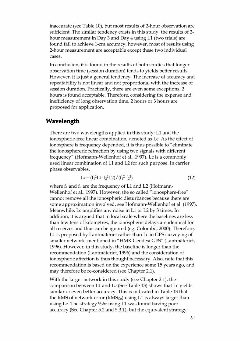
9s6rc using the same method but using Lc signal is found muchbetter. Except this extreme example, RMSCo using Lc is still smallerby 0.2 to 0.8 mm. But their repeatability, Sco, is similar. Moreover,the mean of C0 ( 0C ) using Lc are found always smaller, showingthe measurements using Lc contain less systematic error than usingL1. RMSSo in the first transformation (fitting to known network)using Lc is similar, and slightly worse than L1 except the extremeexample of 9s6rc. RMSSo of the second transformation (compare thepoints of 9000-series to their known height) using Lc is much worsethan using L1 (See Table 13). That means the systematic error of thenetwork using Lc is smaller, but the error in each individual site islarger. This phenomenon coincides with the theory that Lc partlyeliminates ionosphereric affection but amplify the noise.

TableTableTableTable 13.13.13.13. A comparison of the results between L1 and Lc, session durationof 3 hours

Session Diff. RMS of Networkfitting*

(ΔRMSso, mm)

Diff. local height error* (mm)

ΔRMSco ΔSco Δ(Max-Min)

ΔMean ΔRMSso

Leica antenna, 9 sitess, 6 receivers 3.1 3.2 3.8 13.3 0.3 -1.4

Leica antenna, D1, 11 points 0.1 0.2 -0.4 -0.5 0.3 -0.6

Leica antenna, D2, 11 points -0.3 0.3 -0.1 -0.7 0.3 -1.5

DM antenna, D3, 11 points 0.4 0.8 0.1 -0.4 0.8 0.2

DM antenna, D4, 11 points -0.5 0.8 0.6 2.6 0.7 -0.3

Mean value except 9s6r & 9s6rc -0.08 0.53 0.05 0.25 0.53 -0.55

Note: the differences are calculated by the indicators using L1 minus thecorresponding indicators using Lc.

In conclusion, this study shows that it has the potential to achievesimilar or practically even better accuracy with Lc combination,which is contrary with the former proposal. However, it is notenough to conclude that Lc is better than L1 here with only fourpairs of comparisons and measurement of 4 days at the same timeof a year. The following elements might effect the choice ofwavelength: firstly the length of baseline: it is argued that withshort baselines, the atmospheric effect is insignificant (Colombo,2000). Secondly, the magnitude and condition of ionospherericrefraction, which directly determined by the intensity of ionization,see Chapter 6.2.2.

Thus, based on relevant study and the default settings of thesoftware TTC, it is suggested that L1 is better for baselines less than5 km; while Lc is proposed for baselines longer than 5 km. As to theeffect of time, more study on the ionosphere is needed.

33

AntennaAntennaAntennaAntenna

There are three types of antennas applied in this study: LeicaLEIAX1202GG is used on the first and the second day on all sites.On the third and the forth day, Javad JNSCR_C-146-22-1 andAshtech copies of the Dorne Margolin Model T are both applied ondifferent sites as listed in Table 2. These choke-ring antennas withDorne Margolin antenna elements are expected to get better resultas they are more scientific antennas. However, the result turns to beunexpected that commercial standard antennas (here LeicaLEIAX1202GG) gives better result.

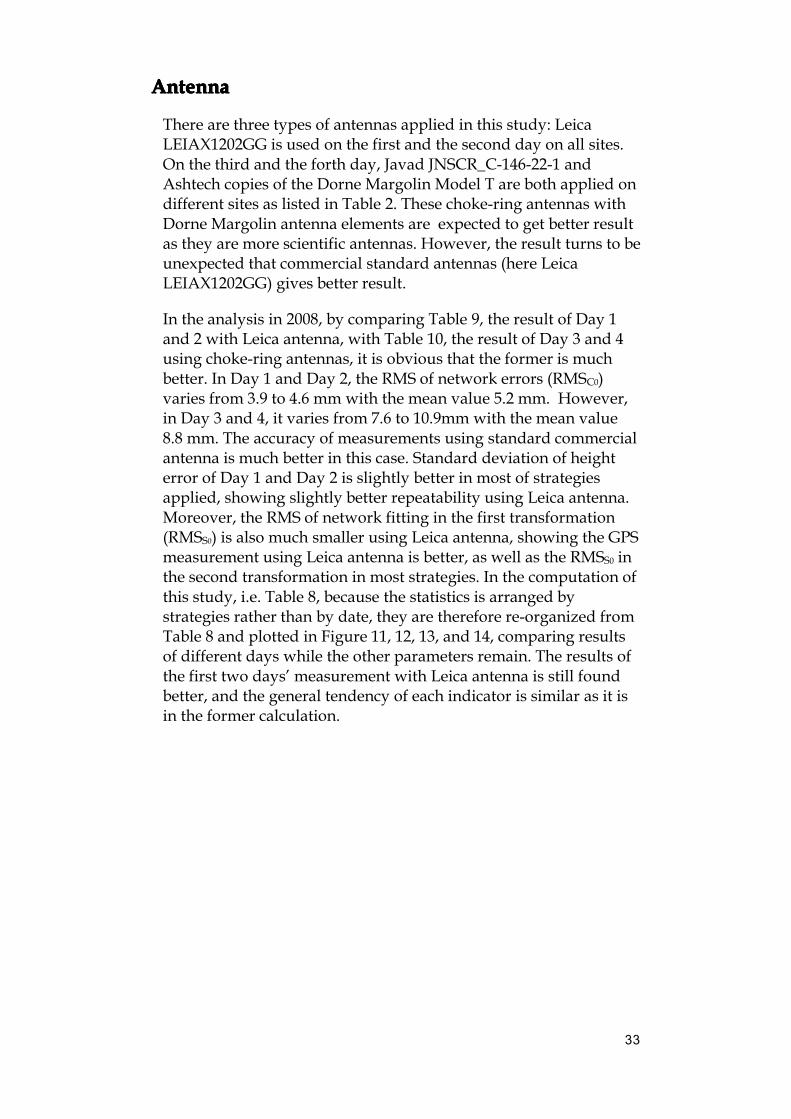
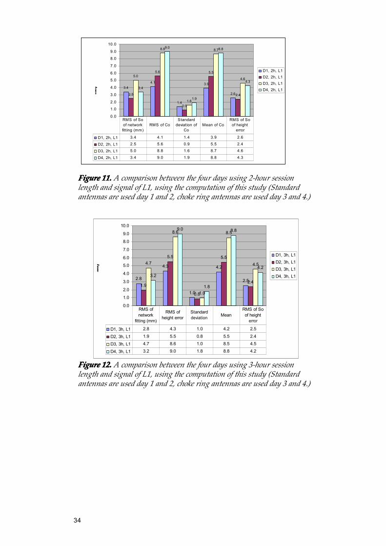
In the analysis in 2008, by comparing Table 9, the result of Day 1and 2 with Leica antenna, with Table 10, the result of Day 3 and 4using choke-ring antennas, it is obvious that the former is muchbetter. In Day 1 and Day 2, the RMS of network errors (RMSC0)varies from 3.9 to 4.6 mm with the mean value 5.2 mm. However,in Day 3 and 4, it varies from 7.6 to 10.9mm with the mean value8.8 mm. The accuracy of measurements using standard commercialantenna is much better in this case. Standard deviation of heighterror of Day 1 and Day 2 is slightly better in most of strategiesapplied, showing slightly better repeatability using Leica antenna.Moreover, the RMS of network fitting in the first transformation(RMSS0) is also much smaller using Leica antenna, showing the GPSmeasurement using Leica antenna is better, as well as the RMSS0 inthe second transformation in most strategies. In the computation ofthis study, i.e. Table 8, because the statistics is arranged bystrategies rather than by date, they are therefore re-organized fromTable 8 and plotted in Figure 11, 12, 13, and 14, comparing resultsof different days while the other parameters remain. The results ofthe first two days’ measurement with Leica antenna is still foundbetter, and the general tendency of each indicator is similar as it isin the former calculation.

34

3.44.1

1.4

3.9

2.62.5

5.6

0.9

5.5

2.4

5.0

8.8

1.6

8.7

4.6

3.4

9.0

1.9

8.8

4.3

0.0

1.0

2.0

3.0

4.0

5.0

6.0

7.0

8.0

9.0

10.0

(mm)

(mm)

(mm)

(mm)

D1, 2h, L1D2, 2h, L1D3, 2h, L1D4, 2h, L1

D1, 2h, L1 3.4 4.1 1.4 3.9 2.6

D2, 2h, L1 2.5 5.6 0.9 5.5 2.4

D3, 2h, L1 5.0 8.8 1.6 8.7 4.6

D4, 2h, L1 3.4 9.0 1.9 8.8 4.3

RMS of So of network fitting (mm)

RMS of CoStandard

deviation of Co

Mean of CoRMS of So

of height error

FigureFigureFigureFigure 11.11.11.11. A comparison between the four days using 2-hour sessionlength and signal of L1, using the computation of this study (Standardantennas are used day 1 and 2, choke ring antennas are used day 3 and 4.)

2.8

4.3

1.0

4.2

2.51.9

5.5

0.8

5.5

2.4

4.7

8.6

1.0

8.5

4.5

3.2

9.0

1.8

8.8

4.2

0.0

1.0

2.0

3.0

4.0

5.0

6.0

7.0

8.0

9.0

10.0

(mm)

(mm)

(mm)

(mm)

D1, 3h, L1D2, 3h, L1D3, 3h, L1D4, 3h, L1

D1, 3h, L1 2.8 4.3 1.0 4.2 2.5

D2, 3h, L1 1.9 5.5 0.8 5.5 2.4

D3, 3h, L1 4.7 8.6 1.0 8.5 4.5

D4, 3h, L1 3.2 9.0 1.8 8.8 4.2

RMS of network

fitting (mm)

RMS of height error

Standard deviation Mean

RMS of So of height

error

FigureFigureFigureFigure 12.12.12.12. A comparison between the four days using 3-hour sessionlength and signal of L1, using the computation of this study (Standardantennas are used day 1 and 2, choke ring antennas are used day 3 and 4.)

35

2.6

4.3

0.9

4.3

2.51.9

5.4

0.7

5.3

2.3

4.3

6.9

1.5

6.8

4.7

3.9

6.4

2.4

6.0

4.6

0.0

1.0

2.0

3.0

4.0

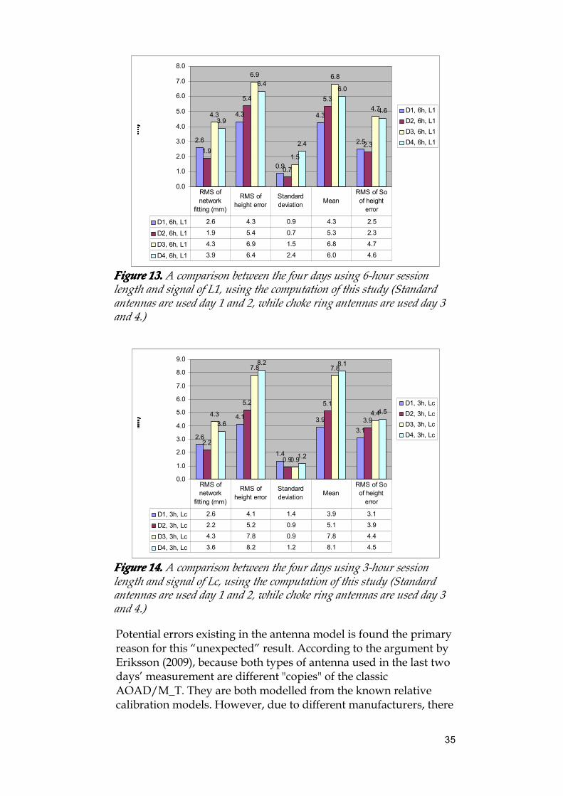
5.0

6.0

7.0

8.0

(mm)

(mm)

(mm)

(mm)

D1, 6h, L1D2, 6h, L1D3, 6h, L1D4, 6h, L1

D1, 6h, L1 2.6 4.3 0.9 4.3 2.5

D2, 6h, L1 1.9 5.4 0.7 5.3 2.3

D3, 6h, L1 4.3 6.9 1.5 6.8 4.7

D4, 6h, L1 3.9 6.4 2.4 6.0 4.6

RMS of network

fitting (mm)

RMS of height error

Standard deviation Mean

RMS of So of height

error

FigureFigureFigureFigure 13.13.13.13. A comparison between the four days using 6-hour sessionlength and signal of L1, using the computation of this study (Standardantennas are used day 1 and 2, while choke ring antennas are used day 3and 4.)

2.6

4.1

1.4

3.93.1

2.2

5.2

0.9

5.1

3.94.3

7.8

0.9

7.8

4.43.6

8.2

1.2

8.1

4.5

0.0

1.0

2.0

3.0

4.0

5.0

6.0

7.0

8.0

9.0

(mm)

(mm)

(mm)

(mm)

D1, 3h, LcD2, 3h, LcD3, 3h, LcD4, 3h, Lc

D1, 3h, Lc 2.6 4.1 1.4 3.9 3.1

D2, 3h, Lc 2.2 5.2 0.9 5.1 3.9

D3, 3h, Lc 4.3 7.8 0.9 7.8 4.4

D4, 3h, Lc 3.6 8.2 1.2 8.1 4.5

RMS of network

fitting (mm)

RMS of height error

Standard deviation Mean

RMS of So of height

error

FigureFigureFigureFigure 14.14.14.14. A comparison between the four days using 3-hour sessionlength and signal of Lc, using the computation of this study (Standardantennas are used day 1 and 2, while choke ring antennas are used day 3and 4.)

Potential errors existing in the antenna model is found the primaryreason for this “unexpected” result. According to the argument byEriksson (2009), because both types of antenna used in the last twodays’ measurement are different "copies" of the classicAOAD/M_T. They are both modelled from the known relativecalibration models. However, due to different manufacturers, there

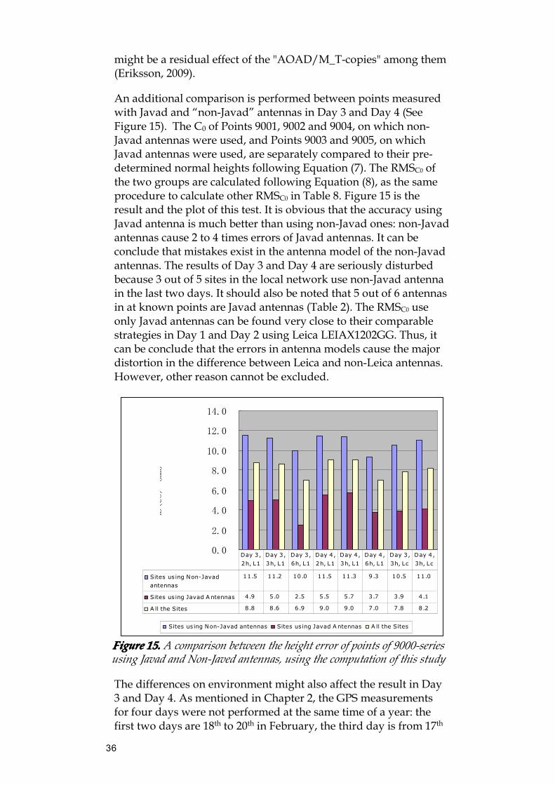
36

might be a residual effect of the "AOAD/M_T-copies" among them(Eriksson, 2009).

An additional comparison is performed between points measuredwith Javad and “non-Javad” antennas in Day 3 and Day 4 (SeeFigure 15). The C0 of Points 9001, 9002 and 9004, on which non-Javad antennas were used, and Points 9003 and 9005, on whichJavad antennas were used, are separately compared to their pre-determined normal heights following Equation (7). The RMSC0 ofthe two groups are calculated following Equation (8), as the sameprocedure to calculate other RMSC0 in Table 8. Figure 15 is theresult and the plot of this test. It is obvious that the accuracy usingJavad antenna is much better than using non-Javad ones: non-Javadantennas cause 2 to 4 times errors of Javad antennas. It can beconclude that mistakes exist in the antenna model of the non-Javadantennas. The results of Day 3 and Day 4 are seriously disturbedbecause 3 out of 5 sites in the local network use non-Javad antennain the last two days. It should also be noted that 5 out of 6 antennasin at known points are Javad antennas (Table 2). The RMSC0 useonly Javad antennas can be found very close to their comparablestrategies in Day 1 and Day 2 using Leica LEIAX1202GG. Thus, itcan be conclude that the errors in antenna models cause the majordistortion in the difference between Leica and non-Leica antennas.However, other reason cannot be excluded.

0.0

2.0

4.0

6.0

8.0

10.0

12.0

14.0

RMS(Co) (mm)

Sites us ing Non-Javad antennas Sites us ing Javad A ntennas A ll the Sites

Sites us ing Non-Javad

antennas

11.5 11.2 10.0 11.5 11.3 9.3 10.5 11.0

Sites us ing Javad A ntennas 4.9 5.0 2.5 5.5 5.7 3.7 3.9 4.1

A ll the Sites 8.8 8.6 6.9 9.0 9.0 7.0 7.8 8.2

Day 3,

2h, L1

Day 3,

3h, L1

Day 3,

6h, L1

Day 4,

2h, L1

Day 4,

3h, L1

Day 4,

6h, L1

Day 3,

3h, Lc

Day 4,

3h, Lc

FigureFigureFigureFigure 11115555.... A comparison between the height error of points of 9000-seriesusing Javad and Non-Javed antennas, using the computation of this study

The differences on environment might also affect the result in Day3 and Day 4. As mentioned in Chapter 2, the GPS measurementsfor four days were not performed at the same time of a year: thefirst two days are 18th to 20th in February, the third day is from 17th

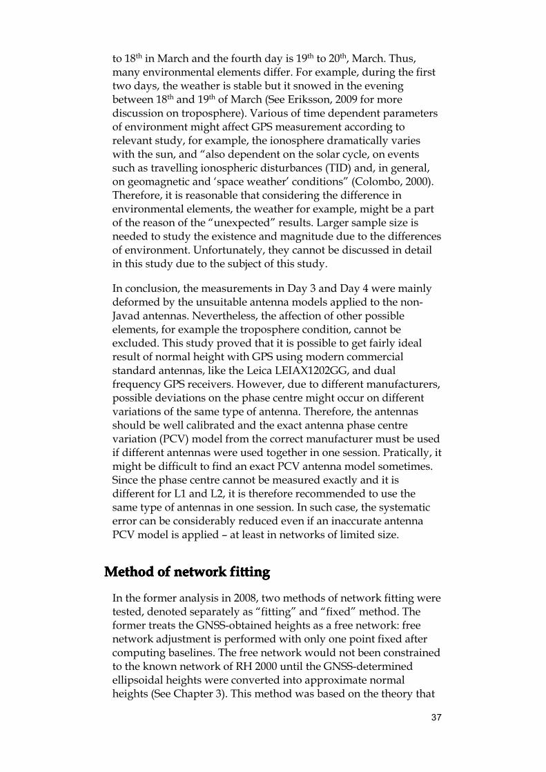
37

to 18th in March and the fourth day is 19th to 20th, March. Thus,many environmental elements differ. For example, during the firsttwo days, the weather is stable but it snowed in the eveningbetween 18th and 19th of March (See Eriksson, 2009 for morediscussion on troposphere). Various of time dependent parametersof environment might affect GPS measurement according torelevant study, for example, the ionosphere dramatically varieswith the sun, and “also dependent on the solar cycle, on eventssuch as travelling ionospheric disturbances (TID) and, in general,on geomagnetic and ‘space weather’ conditions” (Colombo, 2000).Therefore, it is reasonable that considering the difference inenvironmental elements, the weather for example, might be a partof the reason of the “unexpected” results. Larger sample size isneeded to study the existence and magnitude due to the differencesof environment. Unfortunately, they cannot be discussed in detailin this study due to the subject of this study.

In conclusion, the measurements in Day 3 and Day 4 were mainlydeformed by the unsuitable antenna models applied to the non-Javad antennas. Nevertheless, the affection of other possibleelements, for example the troposphere condition, cannot beexcluded. This study proved that it is possible to get fairly idealresult of normal height with GPS using modern commercialstandard antennas, like the Leica LEIAX1202GG, and dualfrequency GPS receivers. However, due to different manufacturers,possible deviations on the phase centre might occur on differentvariations of the same type of antenna. Therefore, the antennasshould be well calibrated and the exact antenna phase centrevariation (PCV) model from the correct manufacturer must be usedif different antennas were used together in one session. Pratically, itmight be difficult to find an exact PCV antenna model sometimes.Since the phase centre cannot be measured exactly and it isdifferent for L1 and L2, it is therefore recommended to use thesame type of antennas in one session. In such case, the systematicerror can be considerably reduced even if an inaccurate antennaPCV model is applied – at least in networks of limited size.

MethodMethodMethodMethod ofofofof networknetworknetworknetwork fittingfittingfittingfitting

In the former analysis in 2008, two methods of network fitting weretested, denoted separately as “fitting” and “fixed” method. Theformer treats the GNSS-obtained heights as a free network: freenetwork adjustment is performed with only one point fixed aftercomputing baselines. The free network would not been constrainedto the known network of RH 2000 until the GNSS-determinedellipsoidal heights were converted into approximate normalheights (See Chapter 3). This method was based on the theory that

38

GNSS observation has relatively high internal accuracy but mightbe tilt as a whole due to errors in GNSS measurement and in geoidmodel. Thus, it is better to firstly ensure the internal accuracy byfree network adjustment, and then fit the internally good networkto the known network to absorb the tilt. This is the only method ofnetwork fitting applied in this study. The latter, so called “fixed”method, constraints the GNSS-obtained network to the knownnetwork of RH 2000 directly in network adjustment using leastsquare adjustment. Practically, it is realized by assigning theknown heights to the benchmarks of national network included inthe GPS measurement during network adjustment so that all thepoints in the national network are fixed in the network adjustmentof the computed GPS baselines.

Theoretically, the “fitting” method is proposed for keeping thegood internal accuracy and absorbing the tilt of the GNSSdetermined network (Hofmann-Wellenhof et al., 1997). Therefore, itis believed better and proposed (Lantmäteriet, 1996). However,according to the statistics of the former analysis in 2008, the “fixed”method yields even better accuracy. In Table 14, the indicators ofusing both methods are compared: two equivalent strategies withthe same settings except the method of network fitting arecompared. Indicators using “fitting” minus the indicators using“fixed”, obtain their differences. Generally, the result shows that“fixed” method gives better overall accuracy (RMSC0) for all thestrategies, 1.5 mm by average. However, the differences of SC0 and(Max-Min) shows that free network fitting have similar, or evenslightly better precision. Generally, this study shows the “fitting”method might not always be the optimum option.

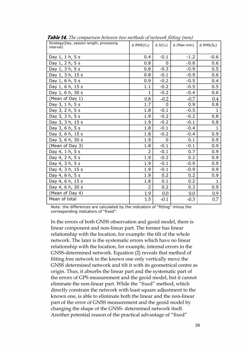
39

TableTableTableTable 14.14.14.14. The comparison between two methods of network fitting (mm)Strategy(Day, session length, processinginterval) Δ RMS(C0) Δ S(C0) Δ (Max-min) Δ RMS(S0)

Day 1, 1 h, 5 s 0.4 -0.1 -1.2 -0.6Day 1, 2 h, 5 s 0.8 0 -0.8 0.6Day 1, 3 h, 5 s 0.8 -0.3 -0.9 0.5Day 1, 3 h, 15 s 0.8 -0.1 -0.9 0.6Day 1, 6 h, 5 s 0.9 -0.2 -0.5 0.4Day 1, 6 h, 15 s 1.1 -0.2 -0.5 0.5Day 1, 6 h, 30 s 1 -0.2 -0.4 0.6(Mean of Day 1) 0.8 -0.2 -0.7 0.4Day 3, 1 h, 5 s 1.7 0 0.9 0.8Day 3, 2 h, 5 s 1.8 -0.1 -0.5 1Day 3, 3 h, 5 s 1.9 -0.2 -0.2 0.8Day 3, 3 h, 15 s 1.9 -0.2 -0.1 0.8Day 3, 6 h, 5 s 1.8 -0.1 -0.4 1Day 3, 6 h, 15 s 1.8 -0.2 -0.4 0.9Day 3, 6 h, 30 s 1.9 0 0.1 0.9(Mean of Day 3) 1.8 -0.1 -0.1 0.9Day 4, 1 h, 5 s 2 -0.1 0.7 0.9Day 4, 2 h, 5 s 1.9 -0.2 0.2 0.9Day 4, 3 h, 5 s 1.9 -0.1 -0.9 0.9Day 4, 3 h, 15 s 1.9 -0.1 -0.9 0.9Day 4, 6 h, 5 s 1.9 0.2 0.2 0.9Day 4, 6 h, 15 s 1.8 0.1 0.2 1Day 4, 6 h, 30 s 2 0.2 0.3 0.9(Mean of Day 4) 1.9 0.0 0.0 0.9Mean of total 1.5 -0.1 -0.3 0.7Note: the differences are calculated by the indicators of “fitting” minus thecorresponding indicators of “fixed”.

In the errors of both GNSS observation and geoid model, there islinear component and non-linear part. The former has linearrelationship with the location, for example: the tilt of the wholenetwork. The later is the systematic errors which have no linearrelationship with the location, for example, internal errors in theGNSS-determined network. Equation (2) reveals that method offitting free network to the known one only vertically move theGNSS determined network and tilt it with its geometrical centre asorigin. Thus, it absorbs the linear part and the systematic part ofthe errors of GPS measurement and the geoid model, but it cannoteliminate the non-linear part. While the “fixed” method, whichdirectly constrain the network with least square adjustment to theknown one, is able to eliminate both the linear and the non-linearpart of the error of GNSS measurement and the geoid model bychanging the shape of the GNSS- determined network itself.Another potential reason of the practical advantage of “fixed”

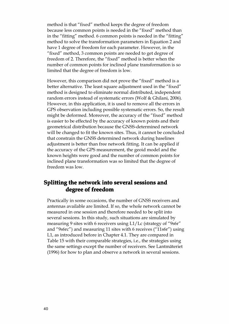
40

method is that “fixed” method keeps the degree of freedombecause less common points is needed in the “fixed” method thanin the “fitting” method. 6 common points is needed in the “fitting”method to solve the transformation parameters in Equation 2 andhave 1 degree of freedom for each parameter. However, in the“fixed” method, 3 common points are needed to get degree offreedom of 2. Therefore, the “fixed” method is better when thenumber of common points for inclined plane transformation is solimited that the degree of freedom is low.

However, this comparison did not prove the “fixed” method is abetter alternative. The least square adjustment used in the “fixed”method is designed to eliminate normal distributed, independentrandom errors instead of systematic errors (Wolf & Ghilani, 2006).However, in this application, it is used to remove all the errors inGPS observation including possible systematic errors. So, the resultmight be deformed. Moreover, the accuracy of the “fixed” methodis easier to be effected by the accuracy of known points and theirgeometrical distribution because the GNSS-determined networkwill be changed to fit the known sites. Thus, it cannot be concludedthat constrain the GNSS determined network during baselinesadjustment is better than free network fitting. It can be applied ifthe accuracy of the GPS measurement, the geoid model and theknown heights were good and the number of common points forinclined plane transformation was so limited that the degree offreedom was low.

SplittingSplittingSplittingSplitting thethethethe networknetworknetworknetwork intointointointo severalseveralseveralseveral sessionssessionssessionssessions andandandanddegreedegreedegreedegree ofofofof freedomfreedomfreedomfreedom

Practically in some occasions, the number of GNSS receivers andantennas available are limited. If so, the whole network cannot bemeasured in one session and therefore needed to be split intoseveral sessions. In this study, such situations are simulated bymeasuring 9 sites with 6 receivers using L1/Lc (strategy of “9s6r”and “9s6rc”) and measuring 11 sites with 6 receives (“11s6r”) usingL1, as introduced before in Chapter 4.1. They are compared inTable 15 with their comparable strategies, i.e., the strategies usingthe same settings except the number of receivers. See Lantmäteriet(1996) for how to plan and observe a network in several sessions.

41

TableTableTableTable 11115555.... Comparison between the spitted network and the original one

Session NameRMS ofnetwork fitting(RMSso, mm)

Local Network Error (mm)RMS ofheight error(RMSco)

Standarddeviation(Sco)

Max –min Mean

RMS of standarderror of unitweight (RMSso)

Leica antenna, L111 points, 6 receivers(11s6r)

7.8 5.5 4.1 14.3 3.8 2.8

Leica antenna, L19 points, 6 receivers(9s6r)

5.7 7.0 6.5 23.1 3.0 2.8

Leica antenna, L19 points, 6 receivers(9s6r_c)

2.6 3.8 2.7 9.9 2.8 4.3

Day 1, Leica antenna, L1,11 points (D1_L1_1000) 2.8 4.3 1.0 3.1 4.2 2.5Day 2, Leica antenna, L1,11 points (D2_L1_1000) 1.9 5.5 0.8 2.1 5.5 2.4Day 1, Leica antenna, Lc,11 points (D1_Lc_1000) 2.6 4.1 1.4 3.6 3.9 3.1Day 2, Leica antenna, Lc,11 points (D2_Lc_1000) 2.2 5.2 0.9 2.8 5.1 3.9

The method measuring 11 sites with 6 receives (11s6r) achieves agood accuracy but with relatively poor repeatability (See Table 15):the RMSCo using “11s6r” is found slightly worse by 1.2 mm thanusing “D1_L1_1000”, but as good as using “D2_L1_1000”. However,SCo using “11s6r" is worse by 3.1 mm than using “D1_L1_1000” andby 3.3 mm than using “D2_L1_1000”. The worse reliability is alsoindicated with the larger absolute values of maximum/minimumof C0 and larger differences between them using “11s6r” (See Table

8 and Table 15). However, the mean of C0 ( 0C ) using “11s6r” iseven better than using “D1_L1_1000” and “D2_L1_1000”, showingthat the extra error is random, rather than systematic. Therefore, itis thought possible to obtain good accuracy by measuring 11 siteswith 6 receivers, but the repeatability is worse because of the lowdegree of freedom due to less redundancy of common points. Theaffection of degree of freedom will be analyzed later in this chapter.With declining of participating sites to 9, the accuracy andrepeatability further decrease. The strategy “9s6r” yields worseresult than “11s6r” by 1.5 mm in RMSCo, by 2.4 mm in SCo, by 0.8

mm in Co (see Table 15). Considering the SCo and RMSCocomprehensively, the final accuracy using “9s6r” might be largerthan 1 cm (1σ)1. Therefore, this strategy is not recommended. The 9sites included in this study has been selected so 6 sites are knownpoints in the national height network, while 3 are sites in the localnetwork. This is in order to keep the degree of freedom in the fit(inclined plane) to the national network at an acceptable level (dof:6-3=3), and at the same time have redundancy in the connection ofthe local network to the GPS-determined points using the 1parameter vertical transformation (dof: 3-1=2).

42

In the first (inclined plane) transformation, in which the desiredheights of the local network is corrected, the degree of freedom isimportant to estimate the unknowns in Equation (2) moreaccurately. According to Equation (2), this transformation needs atleast 3 common points to solve the unknowns. The redundanciesenable averaging out the affection of a single point. With lessredundancy, the estimates of those coefficients are more easilyaffected by error of a single point. Such misestimate of coefficientssubsequently causes larger errors in one session and yields worserepeatability between different sessions (See Table 15). It is alsoshown in this comparison that the measurement with wavelengthLc is better when the degree of freedom is lower, see Table 15.

In conclusion, it is proved feasible to measure the network inseveral sessions and reach 1-cm accuracy although it is not asaccurate and precise as measuring in one session. It is important tokeep more degree of freedom to have better accuracy andprecession, especially when the network cannot be measured inone session. When the degree of freedom is low, it is worthconsidering constraining the GPS determined network directly tothe known one with least square adjustment, i.e., using the so-called “fixed” method, instead of the free network transformation.See Chapter 5.3.4. Unfortunately, it is difficult to specify whichkind of split is acceptable or how to “safely” split the network withthe limitation of data and purpose in this study. It is necessary tohave serious consideration and evaluation when the network has tobe split in several sessions.

TheTheTheThe selectionselectionselectionselection ofofofof commoncommoncommoncommon pointspointspointspoints

As introduced in Chapter 3 and Chapter 5.3.4, GPS-obtainednetwork is firstly treated as a free network and subsequently fittedto the known heights of RH 2000. Common points between the twonetworks are needed to estimate translation value and rotationangles in Equation (2). Their accuracy effects the accuracy of theGPS-determined heights of the local network.

In this study, some benchmarks of RH 2000 included in the GPSmeasurement are used as common points. They are points of “1000-series” in most strategies. However, a trial with points of “2000-series” as common points is performed and compared to itscomparable strategy to study possible errors due to inaccuracy ofthe known points (see Table 16).

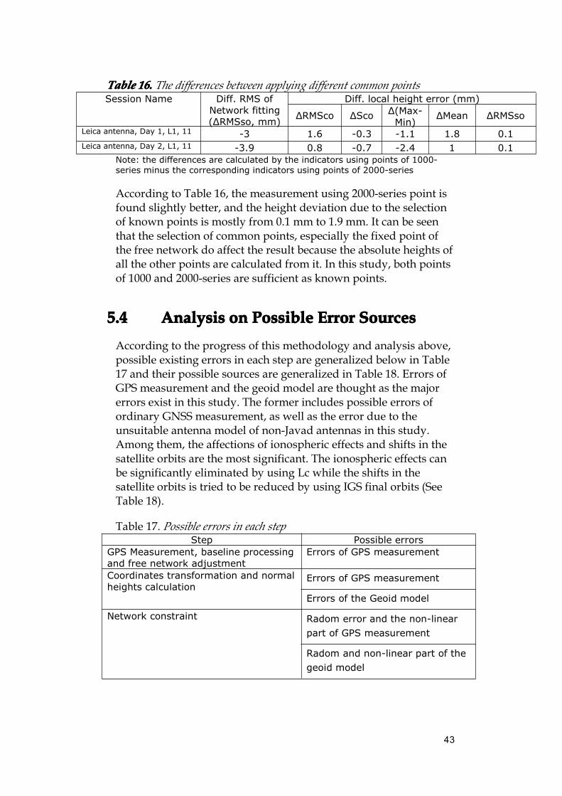
43

TableTableTableTable 11116666.... The differences between applying different common pointsSession Name Diff. RMS of

Network fitting(ΔRMSso, mm)

Diff. local height error (mm)

ΔRMSco ΔSco Δ(Max-Min)

ΔMean ΔRMSso

Leica antenna, Day 1, L1, 11 -3 1.6 -0.3 -1.1 1.8 0.1Leica antenna, Day 2, L1, 11 -3.9 0.8 -0.7 -2.4 1 0.1

Note: the differences are calculated by the indicators using points of 1000-series minus the corresponding indicators using points of 2000-series

According to Table 16, the measurement using 2000-series point isfound slightly better, and the height deviation due to the selectionof known points is mostly from 0.1 mm to 1.9 mm. It can be seenthat the selection of common points, especially the fixed point ofthe free network do affect the result because the absolute heights ofall the other points are calculated from it. In this study, both pointsof 1000 and 2000-series are sufficient as known points.

5.45.45.45.4 AnalysisAnalysisAnalysisAnalysis onononon PossiblePossiblePossiblePossible ErrorErrorErrorError SourcesSourcesSourcesSourcesAccording to the progress of this methodology and analysis above,possible existing errors in each step are generalized below in Table17 and their possible sources are generalized in Table 18. Errors ofGPS measurement and the geoid model are thought as the majorerrors exist in this study. The former includes possible errors ofordinary GNSS measurement, as well as the error due to theunsuitable antenna model of non-Javad antennas in this study.Among them, the affections of ionospheric effects and shifts in thesatellite orbits are the most significant. The ionospheric effects canbe significantly eliminated by using Lc while the shifts in thesatellite orbits is tried to be reduced by using IGS final orbits (SeeTable 18).

Table 17. Possible errors in each stepStep Possible errors

GPS Measurement, baseline processingand free network adjustment

Errors of GPS measurement

Coordinates transformation and normalheights calculation

Errors of GPS measurement

Errors of the Geoid model

Network constraint Radom error and the non-linearpart of GPS measurement

Radom and non-linear part of thegeoid model

44

Table 18. Possible error sources

Errors Error Sources Solution*Errors of GPSmeasurement

Errors in AntennaModels

Use the exact antennamodel, or use the sametype of antenna in onesession

Ionospheric effects Using LcShifts in the satelliteorbits

Using IGS final orbits.Include one known site.

Clock errors of thesatellites' clocks

Double differencing

Multipath effect How to select points!Tropospheric effects Long observation timeOthers

Errors of the GeoidmodelOther possible errors Errors of the known

pointsTry with another set ofknown points

*Note: All the 3 errors may contain linear and non-linear component. Grosserrors are checked and eliminated in each step; the linear part ofsystematic errors is mostly eliminated in the first (inclined plane)transformation.

The linear part of all sorts of errors are theoretically eliminatedwith the 1-dimentional 3-parameter transformation from the freenetwork to the known one. After this transformation, the followingerrors remain: firstly, non-linear part of errors. They aretheoretically incapable being eliminated by such transformationand therefore remain and contribute to the final errors. This non-linear part of errors includes non-linear part of errors in GPSmeasurement and geoid model. Many errors from various sourcesare suspected to be potentially non-linear systematic based onrelevant studies (Colombo, 2000; Hofmann-Wellenhof, et el., 2001etc.), see Table 19. However, due to the limitation of the topic ofthis study, only some of them are proved to be visible in this study.As discussed in Chapter 4.3.1., the existence of such non-linearsystematic errors cause bias in the results and statistics.

TableTableTableTable 11119999.... Possible sources of systematic errorsError Sources Potentially non-linear systematic*Errors in Antenna Models Yes (in this study)Ionospheric effects YesShifts in the satellite orbits InconclusiveClock errors of the satellites' clocks NoMultipath effect InconclusiveTropospheric effects YesErrors of the Geoid model YesErrors of the known points No*Note: Due to the limitation of the topic of this study, some error sources

cannot be studied in detail. Refer to specific studies on such study formore information.

45

6666 ConclusionConclusionConclusionConclusion andandandand DiscussionDiscussionDiscussionDiscussion

6.16.16.16.1 ConclusionConclusionConclusionConclusionBased on the field experiment of GPS measurement in Uppsala, thisstudy evaluated the feasibility, accuracy and the effecting elementsof connecting a local levelling network to RH 2000 with GNSSusing SWEN 08 as geoid model. Essentially, this is determinationof normal heights using GNSS. Different strategies of observationsand computation are evaluated to investigate the effecting elements,with the aim to propose optimum strategies in different conditionsfor future practical applications. Some conclusions from this studyare given below.

It is proved feasible to connect a local levelling network to RH 2000with GPS, i.e., it is possible to obtain accurate normal heights withstatic carrier phase GPS observation and SWEN 08 as geoid model.The accuracy of most strategies tested fulfil the 1-cm level criterion(Chapter 5.2).

The GPS observation is proved sufficient with modern commercialstandard antennas of good quality, like the Leica AX1202 GG, anddual frequency GPS receivers. However, the antennas should bewell calibrated and the exact antenna phase centre variation (PCV)model must be used. Due to different manufacturers, possibledeviations on the phase centre might occur due to the variations ofsame type of antenna (see Chapter 5.3.3). In practical work, it mightbe difficult to find the exact PCV antenna model sometimes. Sincethe phase centre cannot be measured exactly and it is different forL1 and L2, it is better to use the same type of antennas in a session.In such case, the systematic error can be considerably reduced evenif an inaccurate antenna PCV model is applied.

It is shown in this study that session duration of 2 or 3 hours issufficient for the studied application. Longer observation timegenerally yields better result. However, it is not an efficient optionconsidering the accuracy and repeatability will not increaseconstantly and linearly with the increase of observation time(Chapter 5.3.1).

The result using ionospheric-free combination Lc is found as goodas using L1, or even better sometimes in this study, but L1 isproposed in the former studies for smaller network. Consideringthe properties of the affection of ionosphere, L1 is proposed for

46

baselines shorter than approximate 5 km and Lc is thought ideal forbaselines longer than approximate 5 km (Chapter 5.3.2).

The “fixed” method, i.e., directly constrain the GNSS obtainednetwork to the national network in the baseline adjustment, isfound practically better than free network fitting in this studybecause it absorb both the linear and non-linear portion of errors inGPS measurement and the geoid model. However, theoretically, itis unstable because one of the prerequisites of least squareadjustment is to exclude gross and systematic errors. Thus, the“fixed” method might be affected by systematic errors. Moreover, itis more seriously depend on the quality and distribution of knownpoints in the national system than free network fitting because theshape of the GPS-obtained network will be changed to fit theknown coordinates/ heights. However, it is thought to be a betteralternative if there were not so many common points in the first(inclined plane) transformation, because it keeps the degree offreedom (Chapter 5.3.4). A practical procedure may be to firstperform the free network adjustment and inclined planetransformation in order to check for gross errors. When this havebeen checked, perform the network adjustment using fixed heightsat known points.

It is revealed in this study that the accuracy and repeatabilitydecrease when the network is split and measured in severalsessions and when the degree of freedom is low, due to lesscommon sites. With only 3 trials, no “threshold” can be proposedto judge which kind of split is acceptable and how many commonpoints is needed at least. However, it is suggested that such splitshould be considered and evaluated seriously in application whenit is necessary. As to the degree of freedom, at least 3 commonpoints are needed to solve Equation (2) and the necessary degree offreedom is determined by the quality (mainly the magnitude ofnon-linear errors within the GNSS determined network) of theGNSS measurement. Otherwise, constrain the GNSS obtainednetwork directly to the national network, i.e., the “fixed” method,is thought theoretically better when the degree of freedom is low(Chapter 5.2.4 and 5.2.5).

At last, it is proved that the accuracy of the fixed point in the freenetwork and the known sites in the national network will effect theaccuracy of the result. Thus, it is important to apply accurate sitesas fixed point and known points (Chapter 5.3.6 for details).

6.26.26.26.2 DiscussionDiscussionDiscussionDiscussionThe feasibility of GPS normal height obtainment with SWEN 08 isproved and effecting elements are analyzed in this study. Thus, thepredetermined objective is accomplished. However, some

47

limitations found should be discussed; some new problems anduncertainties arose need to be discussed and require furtherinvestigation.

TheTheTheThe uncertaintiesuncertaintiesuncertaintiesuncertainties ofofofof usingusingusingusing LcLcLcLc

In the comparison performed in Chapter 5.3.2 between L1 and Lc,Lc cannot be proved better although it yields better results in thisstudy. The choice of wavelength mainly lies on two aspects: thelength of baselines and the magnitude of both noise andionospheric disturbances, which is uncertain. As to the ionosphere,it dramatically varies with “the main source of ionization”(Colombo, 2000): the sun. The solar cycle, other events such astravelling ionospheric disturbances (TID), in general geomagneticand “space weather” conditions affect tremendously (Colombo,2000). Considering the magnitude of the ionospheric affectionvaries, uncertainties would always exist in the practical result usingLc (Colombo, 2000). In spite of such uncertainties, in this study, it isshowed that the result using Lc is as good as the result using L1,sometimes even better. Such uncertainty of using Lc is a subjectworth further study.

TheTheTheThe limitationlimitationlimitationlimitation ofofofof thisthisthisthis studystudystudystudy andandandand overviewoverviewoverviewoverview onononon thisthisthisthissubjectsubjectsubjectsubject

Firstly, although possible error sources are generalised in Chapter5.4, they are not analyzed into detail. It is believed that there arestill possible errors that remain unclear. For example, the twopossible errors due to errors in horizontal domain mentioned inChapter 3.2 cannot be proved and quantified in this study due tothe limitation on time and subject of this study.

Secondly, the respective magnitude and propagations of each errorand error source, i.e., their contribution to the overall error, remainunclear. Among the error sources listed in Table 18, only the errorsdue to antenna model can be quantified (see Figure 15). In thefurther study, more comparable tests that test each elementseparately while others isolated are required to provide a largersample size. For some error sources that changing with some otherelements, for example atmospheric affection, different set ofobservation in different circumstances should be performed tostudy how it changes. Eventually, each error source and the errorpropagation could be quantified. Such estimation would help tooptimize strategy of observation in the future application. In thisstudy, the result fulfils the criterion of 1-cm accuracy. However,with limitation on measurements available and topic of this study,

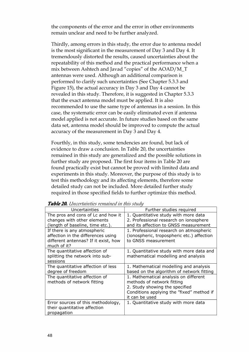
48

the components of the error and the error in other environmentsremain unclear and need to be further analyzed.

Thirdly, among errors in this study, the error due to antenna modelis the most significant in the measurement of Day 3 and Day 4. Ittremendously distorted the results, caused uncertainties about therepeatability of this method and the practical performance when amix between Ashtech and Javad “copies” of the AOAD/M_Tantennas were used. Although an additional comparison isperformed to clarify such uncertainties (See Chapter 5.3.3 andFigure 15), the actual accuracy in Day 3 and Day 4 cannot berevealed in this study. Therefore, it is suggested in Chapter 5.3.3that the exact antenna model must be applied. It is alsorecommended to use the same type of antennas in a session. In thiscase, the systematic error can be easily eliminated even if antennamodel applied is not accurate. In future studies based on the samedata set, antenna model should be improved to compute the actualaccuracy of the measurement in Day 3 and Day 4.

Fourthly, in this study, some tendencies are found, but lack ofevidence to draw a conclusion. In Table 20, the uncertaintiesremained in this study are generalized and the possible solutions infurther study are proposed. The first four items in Table 20 arefound practically exist but cannot be proved with limited data andexperiments in this study. Moreover, the purpose of this study is totest this methodology and its affecting elements, therefore somedetailed study can not be included. More detailed further studyrequired in those specified fields to further optimize this method.

TableTableTableTable 20.20.20.20.Uncertainties remained in this studyUncertainties Further studies required

The pros and cons of Lc and how itchanges with other elements(length of baseline, time etc.).

1. Quantitative study with more data2. Professional research on ionosphereand its affection to GNSS measurement

If there is any atmosphericaffection in the differences usingdifferent antennas? If it exist, howmuch of it?

1. Professional research on atmospheric(ionospheric, tropospheric etc.) affectionto GNSS measurement

The quantitative affection ofsplitting the network into sub-sessions

1. Quantitative study with more data andmathematical modelling and analysis

The quantitative affection of lessdegree of freedom

1. Mathematical modelling and analysisbased on the algorithm of network fitting

The quantitative affection ofmethods of network fitting

1. Mathematical analysis on differentmethods of network fitting2. Study showing the specifiedConditions applying the ”fixed” method ifit can be used

Error sources of this methodology,their quantitative affectionpropagation

1. Quantitative study with more data

49

At least, in this study, only GPS signal is used. That is becausesome receivers used in the GPS field observation campaign wereunable to track GLONASS signals. However, due to their theoreticsimilarity, the general conclusion obtained in this study isapplicable to other systems. Other systems, including GLONASSsignal can be tested in the further study.

50

7777 AcknowledgementsAcknowledgementsAcknowledgementsAcknowledgementsI sincerely express my gratitude to all the people who cared andcontributed to this study. Martin Lidberg at Lantmäteriet and Stig-Göran Mårtensson at the University of Gävle (HiG) gave me thisprecious chance to undertake such study and provided all the helpsas much as they can. Tina Kempe calculated another table ofstatistics separately, helped a lot with patient on the method. Thisstudy can not be accomplished without their kindness, patient andprofessional guidance.

I

ReferencesReferencesReferencesReferencesBecker, J-M., 1985, The Swedish experience with motorized levelling

new techniques and tests, The NAVD Symposium, April pp. 21-26, 1985; Lantmäteriet report number: LMV-RAPPORT 1985:7

Becker, M., Zerbini, S., Baker, T., Bürki, B., Galanis, J., Garate, J.,Georgiev, I., Kahle, H.-G., Kotzev V., Lobazov, V., Marson, I.,Negusini, M., Richter, B., Veis, G. and Yuzefovich, P., 2002.Assessment of height variation by GPS at Mediterranean andBlack Sea coast tide gauges from the SELF projects, Global andPlanetary Change 34(2002) 5-3

Benahmed Daho, S.A., Kahlouche, S., and Fairhead, J.D., 2006. AProcedure for Modelling the Differences Between theGravimetric Geoid Model and GPS/levelling Data with anExample in the North Part of Algeria, Computers &Geosciences 32 (2006) 1733–1745

Colombo, O.L., 2000. Ionospheric Tomography Helps Resolve GPSAmbiguities on the Fly At Distance of Hundreds of KilometersDuring Increased Geomagnetic Activity, IEEE "PLANS 2000"Meeting, San Diego, 13-16 March 2000

Engelis, T., Rapp, R.H. and Tscherning, C.C., 1984. The precisecomputation of geoid undulation differences with comparisonto results obtained from the global positioning system,Geophysical Research Letters, vol. 11, no. 9, pp. 821-824.

Engelis, T., Rapp, R.H. and Bock, Y., 1985. Measuring orthometricheight differences with GPS and gravity data, ManuscriptaGeodaetica, vol. 10, no. 3, pp. 187-194

Eriksson, P., 2009. Anslutning av lokala höjdnät till RH 2000Stomnätsmätning med statisk GNSS-mätning, Projektrapport –ISSN 280-5731 Lantmäteriet ( in Swedish)

Featherstone, W.E., 2008. GNSS-based Heighting in Australia:Current, Emerging and Future Issues, Spatial Science, vol. 53,no. 2, December 2008

Hofmann-Wellenhof, B., Lichtenegger, H. and Collins, J., 2001. GPStheory and practice (Fifth, revised edition), Springer-VerlagWien New York

Hu, W., Sha, Y., and Kuang, S., 2004. New Method for TransformingGlobal Positioning System Height into Normal Height Based on

II

Neural Network, Journal of Surving Engineering, February2004, DOI: 10.1061/(ASCE) 0733-9453(2004) 130:1 (36)

Lantmäteriet 1996. Handbok till mätningskungörelsen Geodesi, GPS(Andra utgåvan), HMK-Ge: GPS, ISBN 91-7774-061-0 (inSwedish). http://www.lantmateriet.se/hmk , cited 03/2011

Lantmäteriet 2009a. Height systems - RH 2000,http://www.lantmateriet.se/templates/LMV_Page.aspx?id=4211, cited 04/2010

Lantmäteriet 2009b. The geoid - Swedish geoid models,http://www.lantmateriet.se/templates/LMV_Page.aspx?id=11011, cited 04/2010

Lantmäteriet 2009c. The user manue of Gtrans 3.63 (in Swedish)

Lilje, M., 2006. The New Swedish Height System RH 2000 and GeoidModel SWEN 05LR, XXIII FIG Congress, Munich, 8-13 October2006

Mårtensson, S-G., 2002. Height Determination by GPS – Accuracywith Respect to Different Geoid Models in Sweden, FIG XXIIInternational Congress, Washington, 19-26 April 2002

Trimble Navigation Ltd., 2002. Trimble Total Control™ User Guide

Wlof, P.R. and Ghilani, C.D., 2006. Elementary Surveying (anintroduction to Geomatics), Pearson Education, Inc. pp. 396 –410

Yang, Z. and Chen, Y., 1999. Determination of Local Geoid withGeometric Method: Case Study, Journal of SurveyingEngineering, August 1999.

Zhang, Q. and Li, J., 2005. The principle and application of GPSsurvey (in Chinese), Science Press of China

Zilkoski, D.B., 1990. Establishing Vertical Control Using GPS SatelliteSurveys, FIG June 1990

Ågren, J., 2009. Beskrivning av de nationella geoidmodellernaSWEN08_RH2000 och SWEN08_RH70 (in Swedish),Rapportserie: Geodesi och Geograkiska informationssystemLMV-Rapport 2009:1

III

AppendixAppendixAppendixAppendix

1.1.1.1. InstallingInstallingInstallingInstalling thethethethe antennaantennaantennaantenna modelsmodelsmodelsmodelsAs mentioned in Chapter 3.1, in this study, the phase centrevariation (PCV) models of Leica AX1202GG and JavadJNSCR_C146-22-1 antennas are not included in TTC. Therefore,they must be manually installed by modifying the file“antenna.ini” (Trimble Navigation Ltd., 2002). The modified fileused in this study is included below.

Antenna.ini

[AntDatabaseInfo]

Version=6.70

Language=SWE

; Instructions

;---------------------------------------------------------------------------

; - Use a unique [key] for each new antenna entry.

; (If you have serial number dependent antenna calibrations this[key]

; must be a combination of antenna name and serial number.)

; - The Type number must be larger than 10000 and unique.

; - The following items must be unique:

; [key]

; Name

; DCName (not needed)

; CharCode (not needed)

; Type

[PhaseCorrTables]

Set1=Trimble,PhaseCorrTable,"Default Trimble Calibration"

Set2=NGS,NGSCorrTable,"US National Geodetic Survey,ant_info.003"

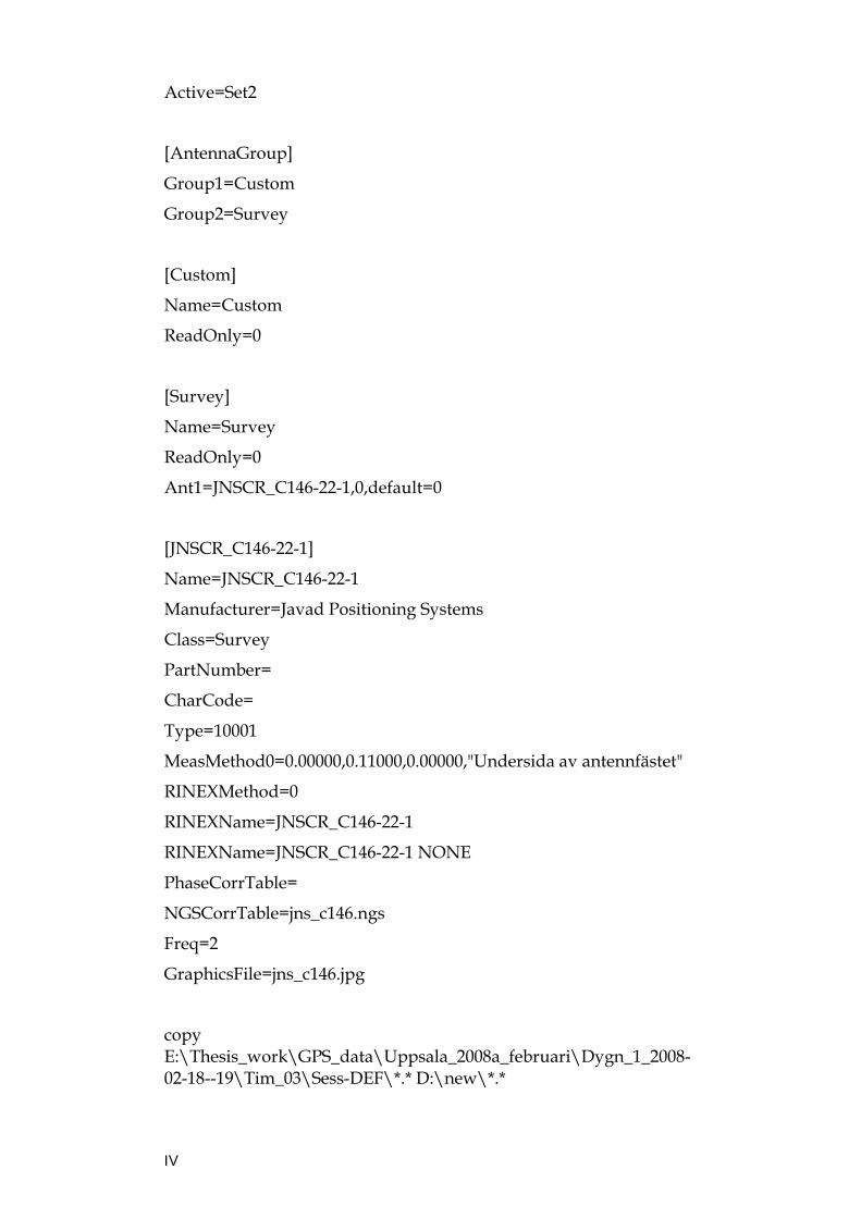
IV

Active=Set2

[AntennaGroup]

Group1=Custom

Group2=Survey

[Custom]

Name=Custom

ReadOnly=0

[Survey]

Name=Survey

ReadOnly=0

Ant1=JNSCR_C146-22-1,0,default=0

[JNSCR_C146-22-1]

Name=JNSCR_C146-22-1

Manufacturer=Javad Positioning Systems

Class=Survey

PartNumber=

CharCode=

Type=10001

MeasMethod0=0.00000,0.11000,0.00000,"Undersida av antennfästet"

RINEXMethod=0

RINEXName=JNSCR_C146-22-1

RINEXName=JNSCR_C146-22-1 NONE

PhaseCorrTable=

NGSCorrTable=jns_c146.ngs

Freq=2

GraphicsFile=jns_c146.jpg

copyE:\Thesis_work\GPS_data\Uppsala_2008a_februari\Dygn_1_2008-02-18--19\Tim_03\Sess-DEF\*.* D:\new\*.*

V

2.2.2.2. RRRRoutineoutineoutineoutine ofofofof thethethethe ExcelExcelExcelExcel VBAVBAVBAVBAmacromacromacromacro usedusedusedused forforforforstatisticsstatisticsstatisticsstatisticsDue to the complexity of file arrangement and Excel operation, anExcel VBA macro is developed to automate some procedures ofstatistics (see Chapter 4.3.2 ). The routine and subs of this macro islisted below.

Private Function FileNames() As Variant

Dim Filter As Variant

Dim DefaultFilter As Integer

Filter = "Text Files (*.txt),*.txt," & "Gtrans Result Files (*.gp),*.gp"

DefaultFilter = 2

'Filter and default settings

' Default Disk and path

ChDrive ("d")

ChDir ("d:\coordinates_results")

'GetOpenFilename

FileNames = Application.GetOpenFilename(Filter, DefaultFilter,"Open Gtrans result files (Translation)...", , True)

End Function

Private Function ReadFile(filenum As Integer) As Variant 'Read thecontent of the file into an array

Dim col As Integer

Dim content(300) As String

col = 1

Do While Not EOF(filenum)

Line Input #1, content(col)

VI

col = col + 1

Loop

ReadFile = content

End Function

Sub RangeWorkSheet()

Columns("A:A").ColumnWidth = 36.5 'adjust width and addheader

Range("A1") = "File Name"

Range("B1") = "So"

Range("D1") = "Co"

Range("E1") = "Session Length"

Columns("A:E").Select

Selection.Sort Key1:=Range("E2"), Order1:=xlAscending,Key2:=Range("A2") _

, Order2:=xlAscending, Header:=xlYes, OrderCustom:=1,MatchCase:=False _

, Orientation:=xlTopToBottom, SortMethod:=xlPinYin,DataOption1:= _

xlSortNormal, DataOption2:=xlSortNormal

End Sub

Sub FillIn(content As Variant, col2 As Integer, fname As String)

Dim filetype As String

filetype = Right$(LCase$(fname), 5)

ActiveCell.Offset(col2) = Trim(fname)

ActiveCell.Offset(col2, 1) = "0" & Mid(Trim(content(28)), 59, 100)

If filetype = "-c.gp" Then

VII

ActiveCell.Offset(col2, 2) = "Co ="

ActiveCell.Offset(col2, 3) = "0" & Mid(Trim(content(33)), 23, 12)

If Mid(Trim(content(33)), 22, 1) = "-" ThenActiveCell.Offset(col2, 3) = ActiveCell.Offset(col2, 3) * -1

End If

ActiveCell.Offset(col2, 4) = InStr(fname, "_") - 3 'count probablesession lenght

End Sub

Sub Compute() 'Compute the current worksheet only

Dim SessionNum As String

Dim i As Integer, RangeStart As Integer, NumRows As Long

Dim CalRange As Range

RangeStart = 2

NumRows = ActiveSheet.UsedRange.Row - 1 +ActiveSheet.UsedRange.Rows.Count 'Poer, How to find the lastrow that contain data in Excel, http://www.excelvbamacro.com,consulted 11/11, 2009

Range("F1") = "Session #" 'header

Range("G1") = "RMS So"

Range("H1") = "RMS Co"

Range("I1") = "Standard Divation Co"

Range("J1") = "Max Co"

Range("K1") = "Min Co"

Range("L1") = "Diff Co"

Range("M1") = "Mean Co"

Range("n1") = "Number of Sessions"

For i = 2 To NumRows

ActiveWorkbook.ActiveSheet.Cells(i, 1).Activate

SessionNum = Left(ActiveCell, 2)

VIII

If SessionNum <> Left(ActiveCell.Offset(1, 0), 2) OrActiveCell.Offset(0, 4) <> ActiveCell.Offset(1, 4) Then

Cells(i, 6) = SessionNum 'fill in the sessionlength

Set CalRange = ActiveSheet.Range(Cells(RangeStart, 2), Cells(i, 2))'range selection

Cells(i, 7).Formula = "=SQRT(SUMSQ(" &CalRange.Columns(1).Address(False, False) & ")/COUNT(" &CalRange.Columns(1).Address(False, False) & "))" 'RMS SoCalculation

Cells(i, 14) = i - RangeStart + 1

If Cells(2, 4) <> "" Then 'if Co exist, Calculate Standard divation,Max, Min, Diff of Co

Set CalRange = CalRange.Offset(0, 2)

Cells(i, 8).Formula = "=SQRT(SumSq(" &CalRange.Columns(1).Address(False, False) & ") / Count(" &CalRange.Columns(1).Address(False, False) & "))"

Cells(i, 9).Formula = "=StDev(" &CalRange.Columns(1).Address(False, False) & ")"

Cells(i, 10).Formula = "=Max(" &CalRange.Columns(1).Address(False, False) & ")"

Cells(i, 11).Formula = "=Min(" &CalRange.Columns(1).Address(False, False) & ")"

ActiveWorkbook.ActiveSheet.Cells(i, 10).Activate

Cells(i, 12).Formula = ActiveCell - ActiveCell.Offset(0, 1)

Cells(i, 13).Formula = "=average(" &CalRange.Columns(1).Address(False, False) & ")"

End If

RangeStart = i + 1

End If

Next i

IX

End Sub

Sub ComputeAll() 'go through and compute all the worksheets

Dim i As Integer

For Each ws In ThisWorkbook.Worksheets

If ws.Name <> "Result" Then

ws.Activate

Call RangeWorkSheet

Call Compute

End If

Next

End Sub

Sub IfExist() 'Look for worksheet "Result", create if it's not exist, toprovide a place for the final result

Dim WorksheetResult As Worksheet

For Each ws In ThisWorkbook.Worksheets 'go through all theworksheets

If ws.Name = "Result" Then

ws.Activate

Exit Sub

End If

Next

Set WorksheetResult = ThisWorkbook.Worksheets.Add

WorksheetResult.Name = "Result"

End Sub

Sub orgnize()

Dim i As Integer, ii As Integer, ComRange As Range

Call IfExist

'ThisWorkbook.Sheets("Result").range("a2").Select

X

With ThisWorkbook.Sheets("Result").Range("a2")

.Offset(0, 0) = "Session Name"

.Offset(0, 1) = "Day"

.Offset(0, 2) = "Session Length"

.Offset(0, 3) = "Number of Sessions"

.Offset(0, 4) = "RMS of network fitting (mm)"

.Offset(0, 5) = "RMS of height error"

.Offset(0, 6) = "Standard deviation"

.Offset(0, 7) = "Max"

.Offset(0, 8) = "Min"

.Offset(0, 9) = "Max - min"

.Offset(0, 10) = "Mean"

.Offset(0, 11) = "RMS of standard error of unit weight"

End With

For Each ws In ThisWorkbook.Worksheets

If ws.Name <> "Result" And Right(ws.Name, 1) = "T" Then

For ii = 2 To ws.UsedRange.Row - 1 +ws.UsedRange.Rows.Count

If ws.Cells(ii, 6) <> "" Then

With ThisWorkbook.Sheets("Result").Range("a3")

.Offset(i, 0) = ws.Cells(ii, 6) '"Session Name"

Select Case ws.Cells(ii, 6) '"Day"

Case 11, 13, 15

.Offset(i, 1) = "1"

Case 12, 14, 16

.Offset(i, 1) = "2"

Case 21, 23

XI

.Offset(i, 1) = "3"

Case 22, 24

.Offset(i, 1) = "4"

Case "9s", 10

.Offset(i, 1) = "1+2"

End Select

.Offset(i, 2) = ws.Cells(ii, 5) '"Session Length"

.Offset(i, 3) = ws.Cells(ii, 14) '"Number of Sessions"

.Offset(i, 5) = ws.Cells(ii, 8) * 1000 '"RMS of height error"

.Offset(i, 6) = ws.Cells(ii, 9) * 1000 'Standard deviation

.Offset(i, 7) = ws.Cells(ii, 10) * 1000 'Max

.Offset(i, 8) = ws.Cells(ii, 11) * 1000 'Min

.Offset(i, 9) = ws.Cells(ii, 12) * 1000 'Max-Min

.Offset(i, 10) = ws.Cells(ii, 13) * 1000 'Mean

.Offset(i, 11) = ws.Cells(ii, 7) * 1000 '"RMS of standard error ofunit weight"

End With

i = i + 1

End If

Next ii

End If

Next

For Each ws In ThisWorkbook.Worksheets

If ws.Name <> "Result" And Right(ws.Name, 1) <> "T" Then

For i = 2 To ws.UsedRange.Row - 1 + ws.UsedRange.Rows.Count

XII

If ws.Cells(i, 6) <> "" Then

For ii = 3 To Worksheets("Result").UsedRange.Row - 1 +Worksheets("Result").UsedRange.Rows.Count

If ws.Cells(i, 6) = Worksheets("Result").Cells(ii, 1) Andws.Cells(i, 5) = Worksheets("Result").Cells(ii, 3) ThenWorksheets("Result").Cells(ii, 5) = ws.Cells(i, 7) * 1000

Next ii

End If

Next i

End If

Next

'the following code format the "result" table and range the result

Columns("B:B").ColumnWidth = 3.44

Columns("C:C").ColumnWidth = 12

Columns("D:D").ColumnWidth = 11.56

Columns("E:E").ColumnWidth = 22

Columns("F:F").ColumnWidth = 16

Columns("G:G").ColumnWidth = 15.11

Columns("H:H").ColumnWidth = 4.56

Columns("I:I").ColumnWidth = 4.78

Range("E3:L27").Select

Range("E27").Activate

Selection.NumberFormat = "0.0"

Range("A2:L27").Select

Selection.Sort Key1:=Range("A3"), Order1:=xlAscending,Key2:=Range("B3") _

, Order2:=xlAscending, Key3:=Range("C3"),Order3:=xlAscending, Header:= _

XIII

xlGuess, OrderCustom:=1, MatchCase:=False,Orientation:=xlTopToBottom, _

DataOption1:=xlSortNormal, DataOption2:=xlSortNormal,DataOption3:= _

xlSortNormal

End Sub

Sub main()

Dim FileName As Variant 'file names

Dim i As Integer, col2 As Integer, sessionlength As Integer, col3 AsInteger 'number of files, number of cols in worksheetInner,SessionLength

col2 = 1

col3 = 1

Dim content As Variant, nameArr As Variant, NeatFileName AsString 'file content

Dim WorkSheetName As String

Dim WorkSheetOuter As Worksheet

Dim WorksheetInner As Worksheet

FileName = FileNames()

If Not IsArray(FileName) Then Exit Sub 'Exit on cancel

Set WorkSheetOuter = Worksheets.Add 'add 2 new worksheets forouter loop and inner points fitting

Set WorksheetInner = Worksheets.Add

For i = LBound(FileName) To UBound(FileName) ' Open Files

Open FileName(i) For Input Access Read As #1

XIV

content = ReadFile(1) 'read files, the content has been read into anarray, and ready for filled into worksheets

'If i = LBound(Filename) Then 'rename 2 worksheets

nameArr = Split(FileName(i), "\")

NeatFileName = nameArr(UBound(nameArr))

'sessionlength = InStr(NeatFileName, "_") - 3 'count probablesession lenght

WorkSheetName = Mid(Trim(NeatFileName), 1, 2)

WorkSheetOuter.Name = WorkSheetName & "_L"

WorksheetInner.Name = WorkSheetName & "_T"

'End If

Select Case Right$(LCase$(FileName(i)), 5)

Case "-c.gp"

WorksheetInner.Activate

Call FillIn(content, col2, NeatFileName)

col2 = col2 + 1

Call RangeWorkSheet

Case "00.gp"

WorkSheetOuter.Activate

Call FillIn(content, col3, NeatFileName)

col3 = col3 + 1

Call RangeWorkSheet

Case Else

MsgBox (FileName(i) & " is not a valid file.")

End Select

Close #1

XV

WorkSheetOuter.Activate

Call RangeWorkSheet

WorksheetInner.Activate

Call RangeWorkSheet

Next i

Set WorkSheetOuter = Nothing

Set WorksheetInner = Nothing

End Sub