Global Positioning Field School Cultural Resources GIS

Washington, DC

MONDAY INTRODUCTION AND COURSE EXPECTATIONS 9:00-9:15 a.m. Seating determines teams for the week. Session 1 OVERVIEW OF GPS CONCEPTS 9:15-10:00 a.m. Format: Lecture After this session, participants will be able to:

- describe the role of satellites in GPS - describe how positions are collected by GPS - recognize sources of error inherent in GPS data - identify effects of selective availability - describe how differential correction works - recognize parameters used in collecting GPS data - understand GPS data structure

BREAK Session 2 GETTING TO KNOW THE GPS EQUIPMENT 10:15 a.m.-Noon Team Leaders Format: Inside/Outside. Direction/Hands-On with GPS units Materials: Manual, GPS units, compass

Exercise 1: Setting Parameters Exercise 2: Locating Active Satellites

After this session, participants will be able to:

- assemble GPS equipment - troubleshoot for bad connections - set data collection parameters - locate active satellites

LUNCH

GPS FIELD SCHOOL 1

Session 3 INTRODUCTION TO DATA COLLECTION 1:30-3:00 p.m. Team Leaders Format: Inside/Outside. Direction/Hands-On with GPS units Materials: GPS units, Crib Card, checklist

Exercise 3: Practicing Data Capture After this session, participants will be able to:

- create, open, and close files - collect generic points, lines, and areas

BREAK Session 4 INTRODUCTION TO PATHFINDER OFFICE SOFTWARE 3:15-5:00 p.m. Format: Lecture and Demonstration/Hands-On with PC Materials: PC, data loggers, null modem cables

Exercise 4: Exploring Pathfinder Office After this session, participants will be able to:

- access software on PC - use Pathfinder Office menus - transfer data between data logger and PC - display and query data on screen

TUESDAY Session 5 PROJECT DEVELOPMENT AND DATA DICTIONARY DESIGN 8:00-10:30 a.m. Format: Lecture/Roundtable Materials: data dictionary work sheets

Exercise 5: Data Dictionary Design After this session, participants will be able to:

- decide the purpose and best method of survey - write a project description to outline the information required - determine the level of accuracy needed for a project - determine what information to collect using GPS - identify features to collect in the field - identify attributes and attribute values for the features

BREAK

2 GPS FIELD SCHOOL

Session 6 ENTERING AND DOWNLOADING THE DATA DICTIONARY 10:45-11:30 a.m. Format: Lecture Materials: PC, data loggers, null modem cables

Exercise 6: Downloading the Data Dictionary After this session, participants will be able to:

- enter data dictionary on PC - download data dictionary to datalogger

LUNCH Session 7 PROJECT FIELDWORK 1:00-4:00 p.m. Team Leaders Format: Teams/Hands-On with GPS units After this session, participants will be able to:

- operate a rover in the field - map features using the data dictionary - maintain a team logbook

WEDNESDAY Session 8 INTRODUCTION TO POST-PROCESSING 8:00-9:00 a.m. Format: Teams/Hands-On with PC Materials: Data loggers and PCs, team logbooks, file inventory forms, null modem cables

Exercise 7: Differential Correction

After this session, participants will be able to: - process base and rover files - conduct differential correction - display field collected data on screen - query their data - fill out file inventory forms

Session 9 INTRODUCTION TO FILE EDITING 9:00-11:30 a.m. Format: Lecture/Demonstration Materials: PCs, team logbooks, file inventory forms After this session, participants will be able to:

- edit features on-screen in Pathfinder Office - use field notebooks to proof data

GPS FIELD SCHOOL 3

LUNCH Session 10 PROJECT FIELDWORK 1:00-4:00 p.m. Team Leaders Format: Teams/Hands-On with GPS units In this session, participants will:

- improve data collection skills - conduct team-based fieldwork - troubleshoot problems

THURSDAY Session 11 POST-PROCESSING AND EDITING 8:00-11:30 a.m. Team Leaders Format: Teams/Hands-On with PC In this session, participants will:

- improve basic processing skills - improve basic editing skills - plot progress on a master map

LUNCH Session 12 PROJECT FIELDWORK 1:00-4:00 p.m. Team Leaders Format: Outside. Teams/Hands-On with GPS units In this session, participants will:

- improve data collection skills - conduct team-based fieldwork

FRIDAY Session 13 POST-PROCESSING AND EDITING 8:00-9:30 a.m. Team Leaders Format: Teams/Hands-On with PC Materials: Data loggers and PCs, team logbooks, file inventory forms In this session, participants will:

- improve basic processing and editing skills - exchange data files with other teams - display data

4 GPS FIELD SCHOOL

BREAK Session 14 EXPORT TO GIS 9:45-10:15 Format: Lecture and Demonstration/Hands-On with PC Materials: PCs, team logbooks, file inventory forms

Exercise 8: Export to GIS Session 15 BASIC GEOGRAPHIC INFORMATION SYSYTEM CONCEPTS 10:20-1:00 After these session, participants will be:

- familiar with the process of exporting data to a GIS - familiar with the data import requirements of ArcView

-familiar with the basics of a Geographic Information Sysytem (GIS) PROJECT DOCUMENTATION AND COURSE EVALUATION 1:00--1:30 p.m. Format: Discussion and awarding of certificates Materials: Team logbooks, file inventory forms, evaluation form

NOTE: ALL IMAGES USED FOR GEOEXPLORER 3 SYSTEM INSTRUCTION COPYRIGHTED TO TRIMBLE NAVIGATION LTD.

Instructors: National Park Service

Cultural Resources GIS 1201 I Street, NW, 2270 Washington, DC 20005 Fax: 202-371-6473

GPS FIELD SCHOOL 5

Session 1: OVERVIEW OF GPS CONCEPTS Global Positioning Systems are tools for navigation and for mapping. The kind of system you should purchase depends on the application you have. Systems vary in looks, price, accuracy and capabilities, but all use the same three things: satellites, receivers and some complicated mathematics to compute coordinate positions for locations on the ground. Each of these components is explained below. Satellites Twenty-eight satellites (SV’s) currently are operational in the GPS constellation, along with two spares in orbit, but not broadcasting signals. The orbits of these satellites are planned so at least 6 SV’s are in view (barring physical blockage on the ground, as from buildings or mountains) at all times anywhere in the world. These satellites are administered and controlled by the US Department of Defense (DOD), but commercial and civilian uses were developed soon after the constellation of satellites was in place. Each satellite is equipped with an atomic clock that is synched to the atomic clocks on all of the other satellites and a radio transmitter. The SV’s are constantly transmitting position (the satellite’s position, not yours) and time data via radio waves. GPS receivers on the ground pick up the radio waves. The radio waves are all around us all of the time, making GPS an open system. If you have the right kind of receiver then you can use DoD’s radio waves free of charge. The orbits of the satellites must be precisely controlled for the system to work. DOD maintains a master control station in Colorado Springs, five monitor stations and three ground antennas throughout the world for the purpose of monitoring the orbits. These stations are constantly reading the position data transmitted by the SV, computing any corrections needed, or future orbit paths, then uploading that information back to the SV. The orbit information is then relayed to individual receivers in the form of an almanac. The almanac is the part of the radio signal containing the satellite orbiting information, and it is used to determine where each satellite is. This almanac or ephemeris information also tells the health of all the satellites. Ephemeris information from one satellite contains information for all of the satellites. The radio signal also contains an identifier, so a receiver can tell which satellite it is tracking. Finally, the radio signal contains time information, although the information that is broadcast is more than a simple time-tag that says 10:52. What is really being broadcast from the each satellite is something called “pseudo-random code.” The pattern of this code is so complex that it seems to be randomly generated. The complexity is important, so that no sections of the code repeat. It is the uniqueness of each segment of code that allows for calculation of time. Each satellite has its own version of the code, and no sections repeat in any of the codes. Receivers

6 GPS FIELD SCHOOL

When the receiver gets signals from a satellite, it can tell what time the signal was transmitted by reading the code. It also knows what time it received the signal. Since radio waves travel at a

constant speed, it is a relatively simple calculation to figure out the distance from the receiver to the satellite. But calculating the distance to the satellite is only part of the problem. Mathematics

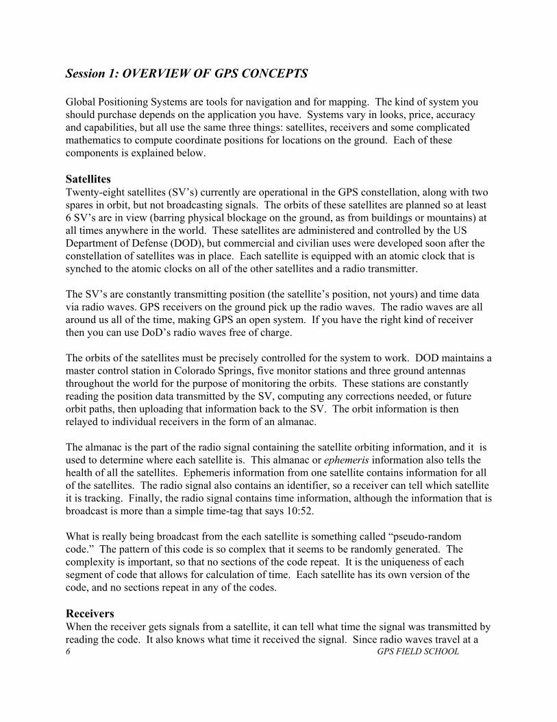
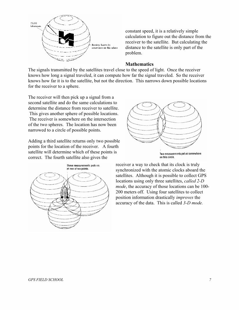
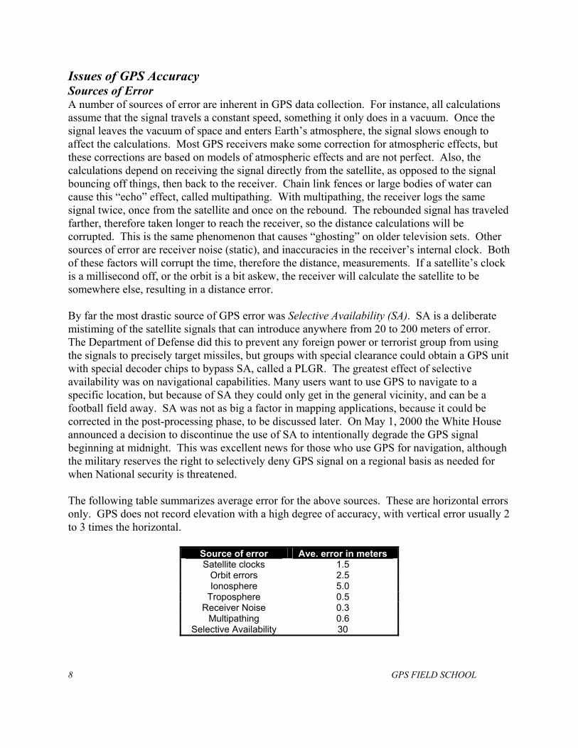
The signals transmitted by the satellites travel close to the speed of light. Once the receiver knows how long a signal traveled, it can compute how far the signal traveled. So the receiver knows how far it is to the satellite, but not the direction. This narrows down possible locations for the receiver to a sphere. The receiver will then pick up a signal from a second satellite and do the same calculations to determine the distance from receiver to satellite. This gives another sphere of possible locations. The receiver is somewhere on the intersection of the two spheres. The location has now been narrowed to a circle of possible points. Adding a third satellite returns only two possible points for the location of the receiver. A fourth satellite will determine which of these points is correct. The fourth satellite also gives the

receiver a way to check that its clock is truly synchronized with the atomic clocks aboard the satellites. Although it is possible to collect GPS locations using only three satellites, called 2-D mode, the accuracy of those locations can be 100-200 meters off. Using four satellites to collect position information drastically improves the accuracy of the data. This is called 3-D mode.

GPS FIELD SCHOOL 7

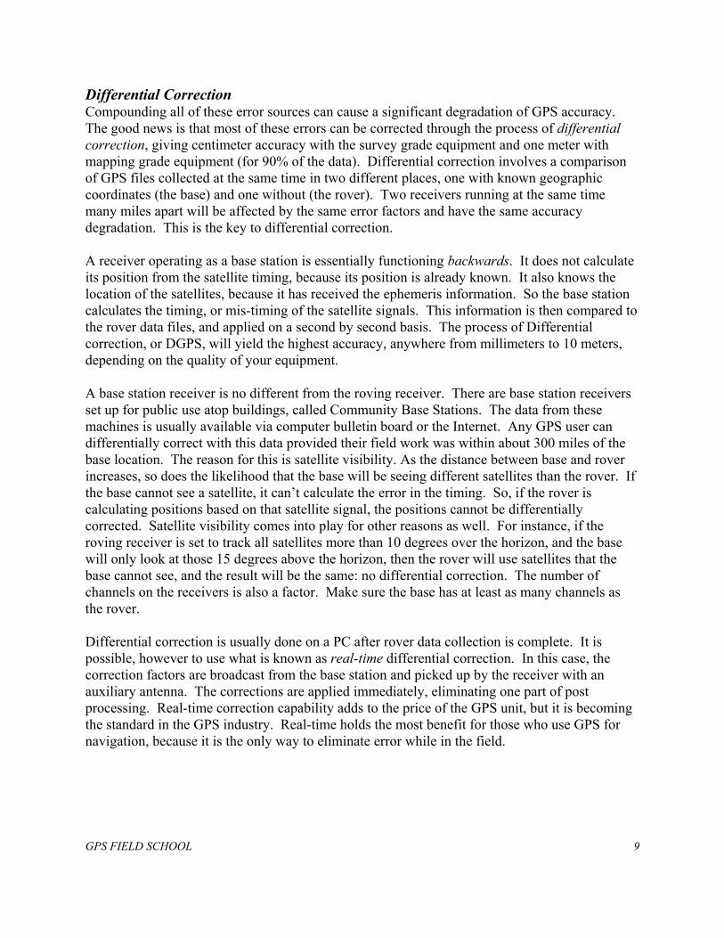
Issues of GPS Accuracy Sources of Error A number of sources of error are inherent in GPS data collection. For instance, all calculations assume that the signal travels a constant speed, something it only does in a vacuum. Once the signal leaves the vacuum of space and enters Earth’s atmosphere, the signal slows enough to affect the calculations. Most GPS receivers make some correction for atmospheric effects, but these corrections are based on models of atmospheric effects and are not perfect. Also, the calculations depend on receiving the signal directly from the satellite, as opposed to the signal bouncing off things, then back to the receiver. Chain link fences or large bodies of water can cause this “echo” effect, called multipathing. With multipathing, the receiver logs the same signal twice, once from the satellite and once on the rebound. The rebounded signal has traveled farther, therefore taken longer to reach the receiver, so the distance calculations will be corrupted. This is the same phenomenon that causes “ghosting” on older television sets. Other sources of error are receiver noise (static), and inaccuracies in the receiver’s internal clock. Both of these factors will corrupt the time, therefore the distance, measurements. If a satellite’s clock is a millisecond off, or the orbit is a bit askew, the receiver will calculate the satellite to be somewhere else, resulting in a distance error. By far the most drastic source of GPS error was Selective Availability (SA). SA is a deliberate mistiming of the satellite signals that can introduce anywhere from 20 to 200 meters of error. The Department of Defense did this to prevent any foreign power or terrorist group from using the signals to precisely target missiles, but groups with special clearance could obtain a GPS unit with special decoder chips to bypass SA, called a PLGR. The greatest effect of selective availability was on navigational capabilities. Many users want to use GPS to navigate to a specific location, but because of SA they could only get in the general vicinity, and can be a football field away. SA was not as big a factor in mapping applications, because it could be corrected in the post-processing phase, to be discussed later. On May 1, 2000 the White House announced a decision to discontinue the use of SA to intentionally degrade the GPS signal beginning at midnight. This was excellent news for those who use GPS for navigation, although the military reserves the right to selectively deny GPS signal on a regional basis as needed for when National security is threatened. The following table summarizes average error for the above sources. These are horizontal errors only. GPS does not record elevation with a high degree of accuracy, with vertical error usually 2 to 3 times the horizontal.

Source of error Ave. error in meters Satellite clocks 1.5

Orbit errors 2.5 Ionosphere 5.0

Troposphere 0.5 Receiver Noise 0.3

Multipathing 0.6 Selective Availability 30

8 GPS FIELD SCHOOL

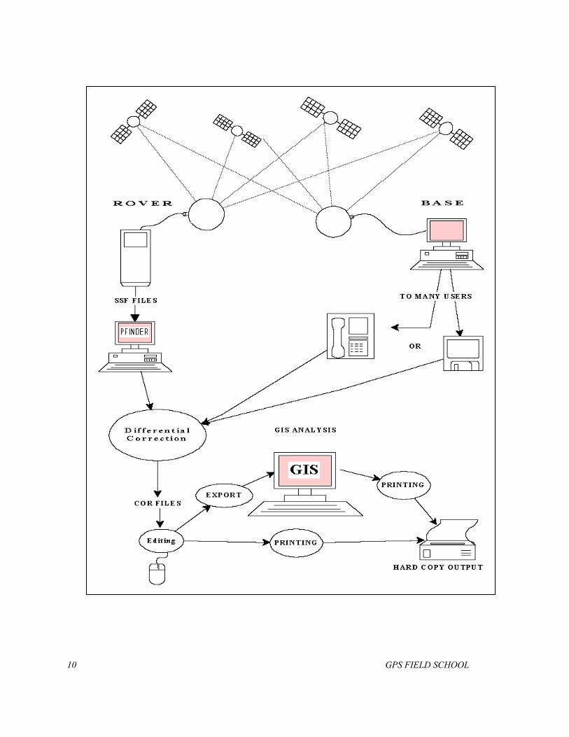
Differential Correction Compounding all of these error sources can cause a significant degradation of GPS accuracy. The good news is that most of these errors can be corrected through the process of differential correction, giving centimeter accuracy with the survey grade equipment and one meter with mapping grade equipment (for 90% of the data). Differential correction involves a comparison of GPS files collected at the same time in two different places, one with known geographic coordinates (the base) and one without (the rover). Two receivers running at the same time many miles apart will be affected by the same error factors and have the same accuracy degradation. This is the key to differential correction. A receiver operating as a base station is essentially functioning backwards. It does not calculate its position from the satellite timing, because its position is already known. It also knows the location of the satellites, because it has received the ephemeris information. So the base station calculates the timing, or mis-timing of the satellite signals. This information is then compared to the rover data files, and applied on a second by second basis. The process of Differential correction, or DGPS, will yield the highest accuracy, anywhere from millimeters to 10 meters, depending on the quality of your equipment. A base station receiver is no different from the roving receiver. There are base station receivers set up for public use atop buildings, called Community Base Stations. The data from these machines is usually available via computer bulletin board or the Internet. Any GPS user can differentially correct with this data provided their field work was within about 300 miles of the base location. The reason for this is satellite visibility. As the distance between base and rover increases, so does the likelihood that the base will be seeing different satellites than the rover. If the base cannot see a satellite, it can’t calculate the error in the timing. So, if the rover is calculating positions based on that satellite signal, the positions cannot be differentially corrected. Satellite visibility comes into play for other reasons as well. For instance, if the roving receiver is set to track all satellites more than 10 degrees over the horizon, and the base will only look at those 15 degrees above the horizon, then the rover will use satellites that the base cannot see, and the result will be the same: no differential correction. The number of channels on the receivers is also a factor. Make sure the base has at least as many channels as the rover. Differential correction is usually done on a PC after rover data collection is complete. It is possible, however to use what is known as real-time differential correction. In this case, the correction factors are broadcast from the base station and picked up by the receiver with an auxiliary antenna. The corrections are applied immediately, eliminating one part of post processing. Real-time correction capability adds to the price of the GPS unit, but it is becoming the standard in the GPS industry. Real-time holds the most benefit for those who use GPS for navigation, because it is the only way to eliminate error while in the field.

GPS FIELD SCHOOL 9

10 GPS FIELD SCHOOL

Data Structure All of the data that comes from the receiver is in the form of positions: x, y, and z latitude, longitude, elevation coordinates. Asset Surveyor combines positions into a feature, such as a road or an archeological site. GIS and GPS classify features as one of three types: point, line or area (polygon). Point features are made up of a number of positions averaged together. Because of the averaging, point features are usually the most accurate. Line features are strings of positions joined together chronologically, like connect the dots. Polygon features are like line features, except that the last position connects to the first, forming an enclosed area. The user enters information about the feature; its attributes, such as name of the road or state identification number for the site. Attributes are sometimes in the form of a menu--a list of possible choices for the attribute. Each item on the menu is called an attribute value. A good example is a feature called “road”. The user may want to know about the road surface. However, the user doesn’t need to know in great detail about the surface, only whether it is paved, gravel or earth. In this case, the feature is ROAD, the attribute is surface type, and the attribute values are paved, gravel, or earth. Attributes and positions together make up a feature. The receiver supplies the positions, and the user supplies the attributes from what is called a data dictionary. The data dictionary is defined before the mapping begins and consists of a list of things to be mapped and the information to collect about each one. Features are then stored in a file. The file is downloaded to a PC and processed using Pathfinder Office software. Post-processing occurs in two stages: differential correction and editing. The data does not come out of the datalogger looking perfect. All accuracy statements on GPS equipment are true only 90% of the time. Therefore, the data will need some “tweaking.” Pathfinder Office software allows the users to delete obviously erroneous positions when necessary. It does not allow the user to insert any information from the keyboard or with the mouse. All input can come only from a GPS unit, so how well you use the GPS unit in the field determines how accurate your information will be. Getting the most accurate information The reliability of GPS data depends on three things: 1) The GPS equipment: If you have a 6 channel hand-held receiver you will get decent results.

If you have a 12 channel survey grade receiver, you will get better results. 2) Proper techniques for data collection and editing: There are many things you can do while in

the field to improve the reliability of your data. These will be discussed in a later session. 3) Careful planning and teamwork

GPS FIELD SCHOOL 11

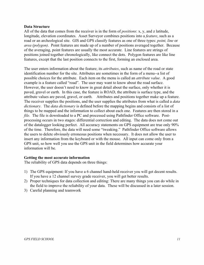
Session 2: GETTING TO KNOW THE GPS EQUIPMENT WHEN USING ASSET SURVEYOR on a TSC-1

Highlight an option and press enter to select it After changing settings or logging a feature, press ENTER to save and exit the screen Use up and down arrows to navigate through menus or else press the first letter of desired

option. Note: if only one item begins with the letter, you will immediately enter that option. Function keys (F1 - F5) have different functions based on the menu you are in. Read the

bottom of the display to determine the uses. Once in a screen setting that has a menu the item can be changed using the right toggle then

the up or down toggle to highlight the menu item, then ENTER to choose the highlighted item.

FIRST EXERCISE: SETTING PARAMETERS FOR THE TRIMBLE PROXR GPS SETTINGS

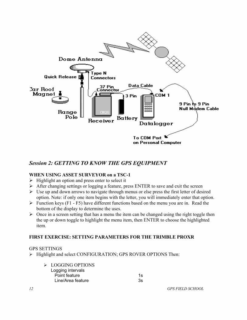
Highlight and select CONFIGURATION; GPS ROVER OPTIONS Then:

LOGGING OPTIONS Logging intervals

Point feature 1s Line/Area feature 3s

12 GPS FIELD SCHOOL

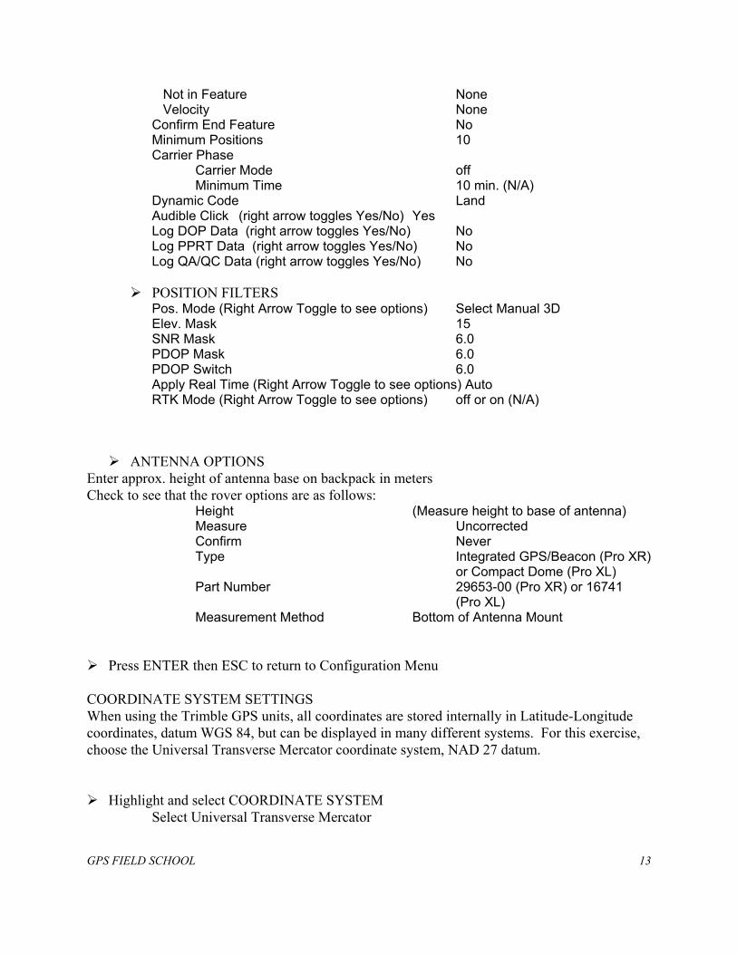
Not in Feature None Velocity None Confirm End Feature No Minimum Positions 10 Carrier Phase Carrier Mode off Minimum Time 10 min. (N/A) Dynamic Code Land Audible Click (right arrow toggles Yes/No) Yes Log DOP Data (right arrow toggles Yes/No) No Log PPRT Data (right arrow toggles Yes/No) No Log QA/QC Data (right arrow toggles Yes/No) No

POSITION FILTERS

Pos. Mode (Right Arrow Toggle to see options) Select Manual 3D Elev. Mask 15 SNR Mask 6.0 PDOP Mask 6.0 PDOP Switch 6.0 Apply Real Time (Right Arrow Toggle to see options) Auto RTK Mode (Right Arrow Toggle to see options) off or on (N/A)

ANTENNA OPTIONS Enter approx. height of antenna base on backpack in meters Check to see that the rover options are as follows:

Height (Measure height to base of antenna) Measure Uncorrected Confirm Never Type Integrated GPS/Beacon (Pro XR)

or Compact Dome (Pro XL) Part Number 29653-00 (Pro XR) or 16741

(Pro XL) Measurement Method Bottom of Antenna Mount

Press ENTER then ESC to return to Configuration Menu

COORDINATE SYSTEM SETTINGS When using the Trimble GPS units, all coordinates are stored internally in Latitude-Longitude coordinates, datum WGS 84, but can be displayed in many different systems. For this exercise, choose the Universal Transverse Mercator coordinate system, NAD 27 datum.

Highlight and select COORDINATE SYSTEM Select Universal Transverse Mercator

GPS FIELD SCHOOL 13

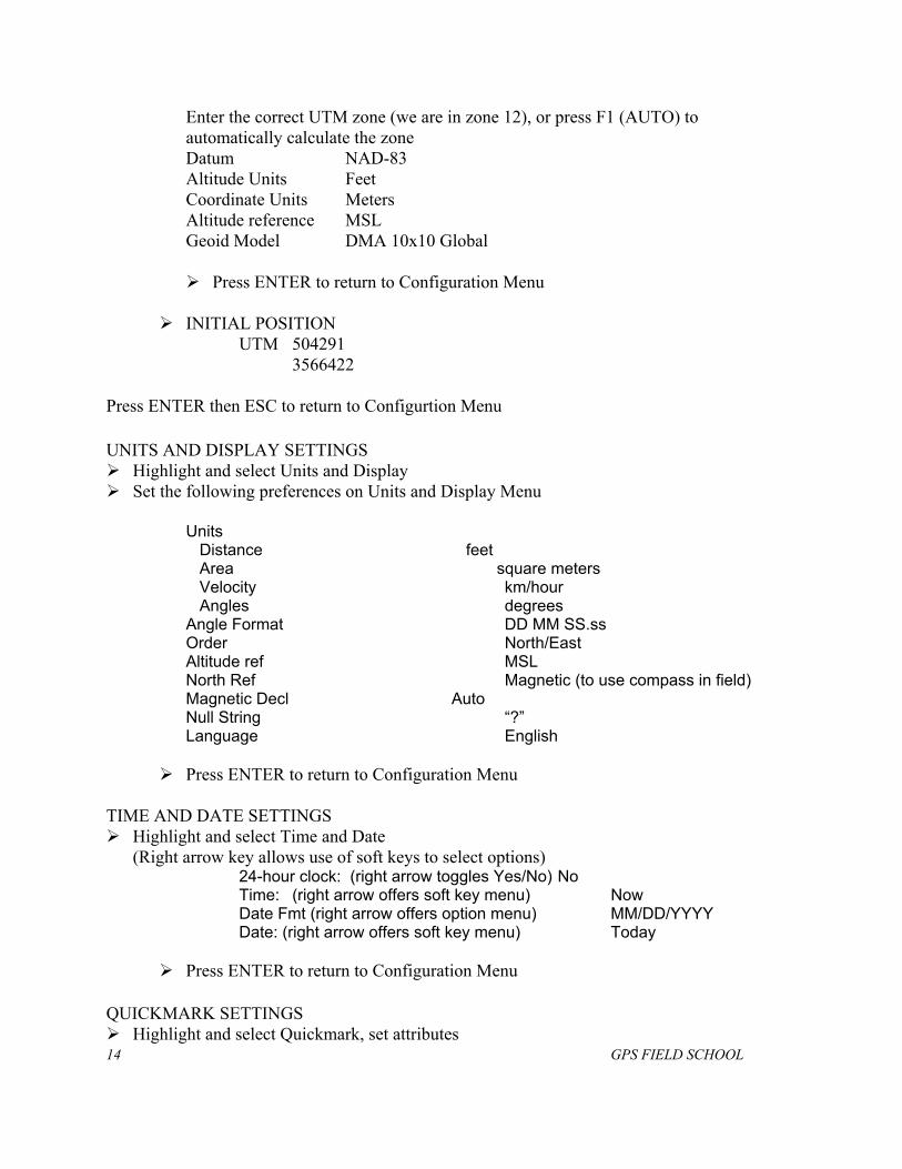
Enter the correct UTM zone (we are in zone 12), or press F1 (AUTO) to automatically calculate the zone

Datum NAD-83 Altitude Units Feet Coordinate Units Meters Altitude reference MSL Geoid Model DMA 10x10 Global

Press ENTER to return to Configuration Menu

INITIAL POSITION

UTM 504291 3566422

P ress ENTER then ESC to return to Configurtion Menu UNITS AND DISPLAY SETTINGS

Highlight and select Units and Display Set the following preferences on Units and Display Menu

Units Distance feet Area square meters Velocity km/hour Angles degrees Angle Format DD MM SS.ss Order North/East Altitude ref MSL North Ref Magnetic (to use compass in field) Magnetic Decl Auto Null String “?” Language English

Press ENTER to return to Configuration Menu

TIME AND DATE SETTINGS

Highlight and select Time and Date (Right arrow key allows use of soft keys to select options)

24-hour clock: (right arrow toggles Yes/No) No Time: (right arrow offers soft key menu) Now Date Fmt (right arrow offers option menu) MM/DD/YYYY Date: (right arrow offers soft key menu) Today

Press ENTER to return to Configuration Menu QUICKMARK SETTINGS

14 GPS FIELD SCHOOL Highlight and select Quickmark, set attributes

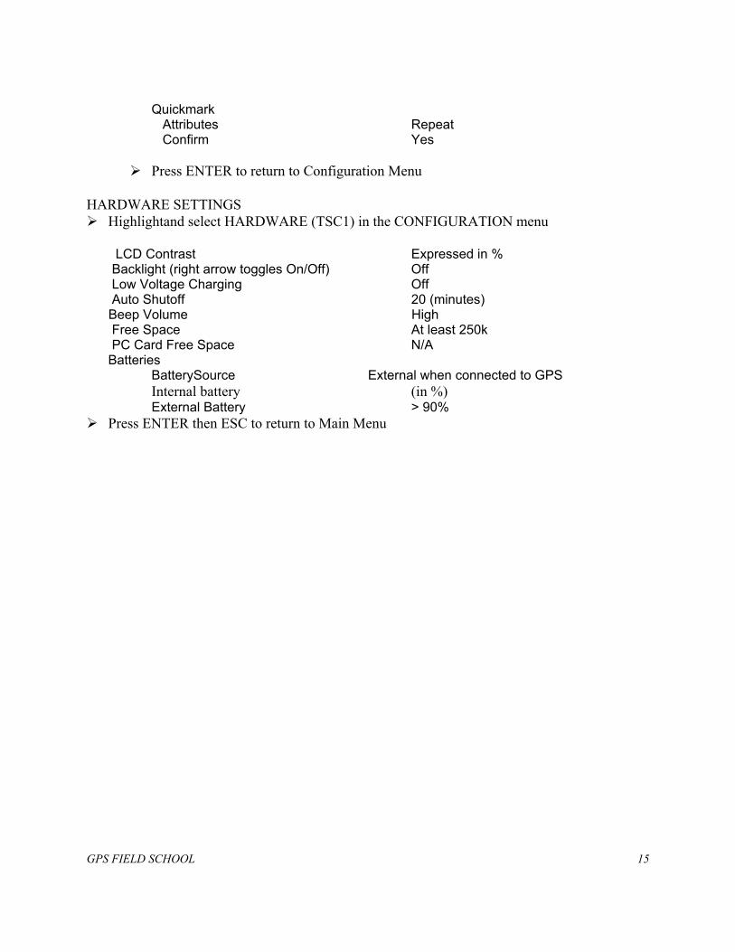
Quickmark Attributes Repeat Confirm Yes

Press ENTER to return to Configuration Menu

HARDWARE SETTINGS Highlightand select HARDWARE (TSC1) in the CONFIGURATION menu

LCD Contrast Expressed in %

Backlight (right arrow toggles On/Off) Off Low Voltage Charging Off Auto Shutoff 20 (minutes)

Beep Volume High Free Space At least 250k PC Card Free Space N/A Batteries

BatterySource External when connected to GPS Internal battery (in %) External Battery > 90%

Press ENTER then ESC to return to Main Menu

GPS FIELD SCHOOL 15

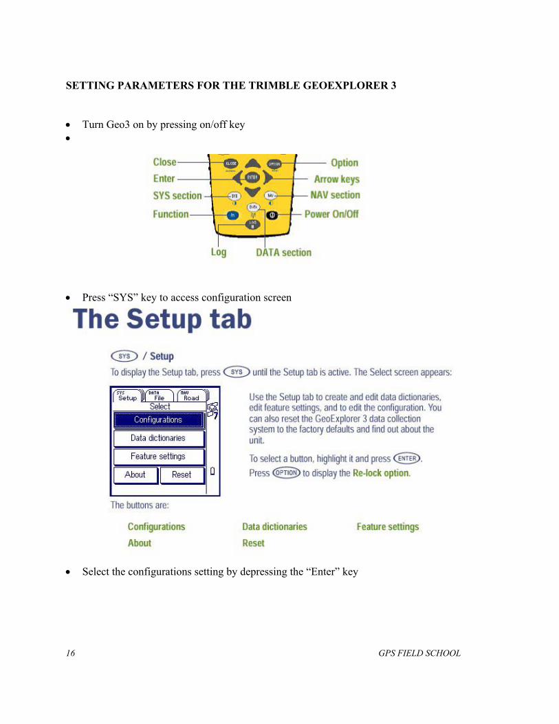
SETTING PARAMETERS FOR THE TRIMBLE GEOEXPLORER 3 • Turn Geo3 on by pressing on/off key •

• Press “SYS” key to access configuration screen

• Select the configurations setting by depressing the “Enter” key

16 GPS FIELD SCHOOL

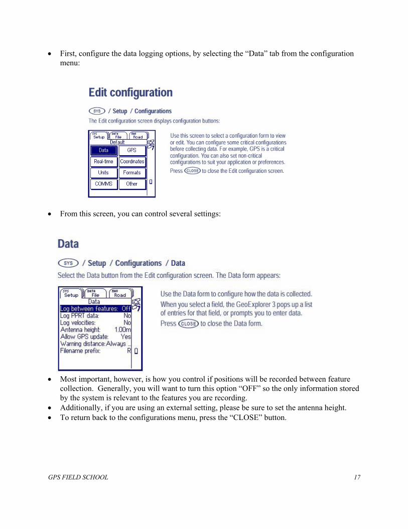
• First, configure the data logging options, by selecting the “Data” tab from the configuration menu:

• From this screen, you can control several settings:

• Most important, however, is how you control if positions will be recorded between feature collection. Generally, you will want to turn this option “OFF” so the only information stored by the system is relevant to the features you are recording.

• Additionally, if you are using an external setting, please be sure to set the antenna height. • To return back to the configurations menu, press the “CLOSE” button.

GPS FIELD SCHOOL 17

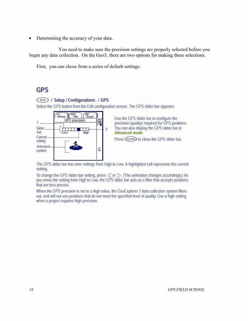
• Determining the accuracy of your data.

You need to make sure the precision settings are properly selected before you begin any data collection. On the Geo3, there are two options for making these selections.

First, you can chose from a series of default settings:

18 GPS FIELD SCHOOL

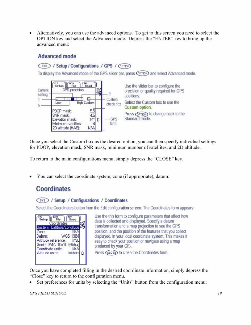
• Alternatively, you can use the advanced options. To get to this screen you need to select the OPTION key and select the Advanced mode. Depress the “ENTER” key to bring up the advanced menu:

Once you select the Custom box as the desired option, you can then specify individual settings for PDOP, elevation mask, SNR mask, minimum number of satellites, and 2D altitude. To return to the main configurations menu, simply depress the “CLOSE” key. • You can select the coordinate system, zone (if appropriate), datum:

Once you have completed filling in the desired coordinate information, simply depress the “Close” key to return to the configuration menu. • Set preferences for units by selecting the “Units” button from the configuration menu: GPS FIELD SCHOOL 19

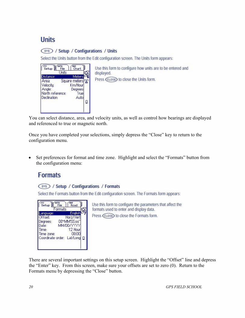
You can select distance, area, and velocity units, as well as control how bearings are displayed and referenced to true or magnetic north. Once you have completed your selections, simply depress the “Close” key to return to the configuration menu. • Set preferences for format and time zone. Highlight and select the “Formats” button from

the configuration menu:

There are several important settings on this setup screen. Highlight the “Offset” line and depress the “Enter” key. From this screen, make sure your offsets are set to zero (0). Return to the Formats menu by depressing the “Close” button.

20 GPS FIELD SCHOOL

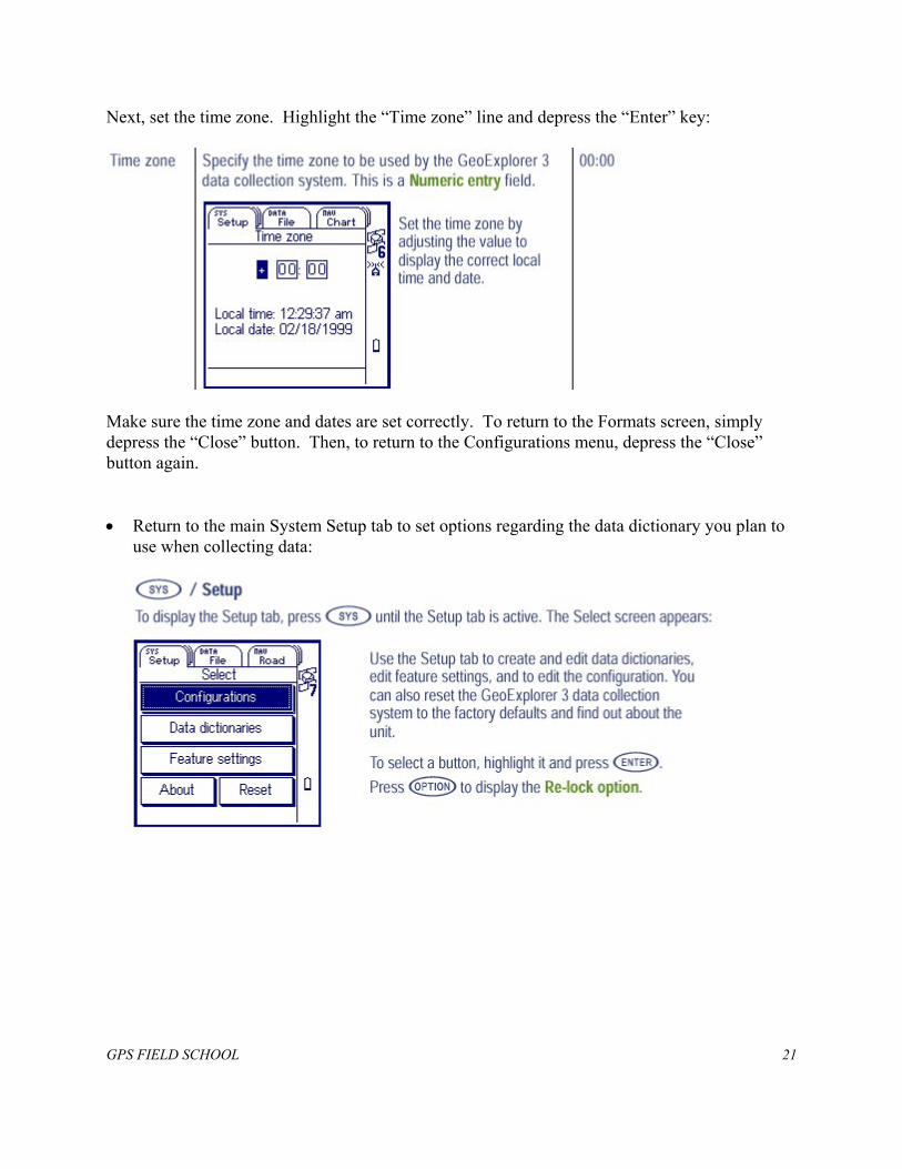
Next, set the time zone. Highlight the “Time zone” line and depress the “Enter” key:

Make sure the time zone and dates are set correctly. To return to the Formats screen, simply depress the “Close” button. Then, to return to the Configurations menu, depress the “Close” button again. • Return to the main System Setup tab to set options regarding the data dictionary you plan to

use when collecting data:

GPS FIELD SCHOOL 21

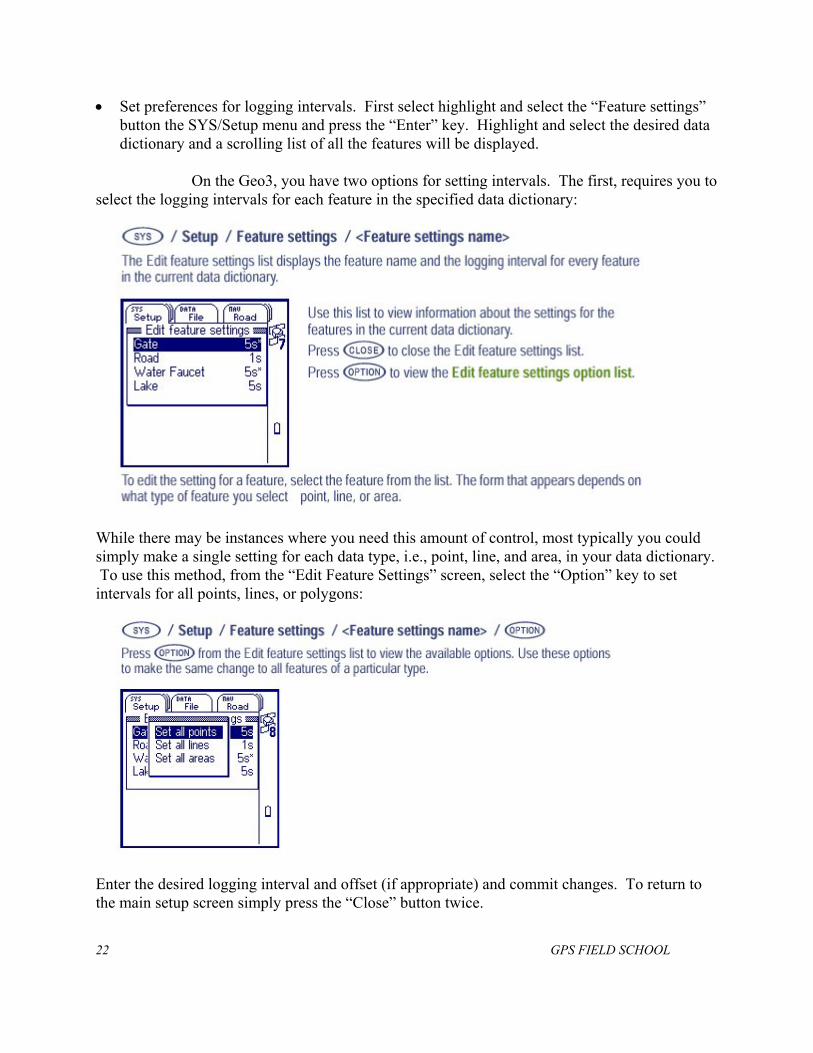
• Set preferences for logging intervals. First select highlight and select the “Feature settings” button the SYS/Setup menu and press the “Enter” key. Highlight and select the desired data dictionary and a scrolling list of all the features will be displayed.

On the Geo3, you have two options for setting intervals. The first, requires you to

select the logging intervals for each feature in the specified data dictionary:

While there may be instances where you need this amount of control, most typically you could simply make a single setting for each data type, i.e., point, line, and area, in your data dictionary. To use this method, from the “Edit Feature Settings” screen, select the “Option” key to set intervals for all points, lines, or polygons:

Enter the desired logging interval and offset (if appropriate) and commit changes. To return to the main setup screen simply press the “Close” button twice.

22 GPS FIELD SCHOOL

SECOND EXERCISE: LOCATING ACTIVE SATELLITES FOR THE TRIMBLE PROXR From Main Menu

Select SATELLITE INFORMATION Press F1 (Mode) to view satellite information

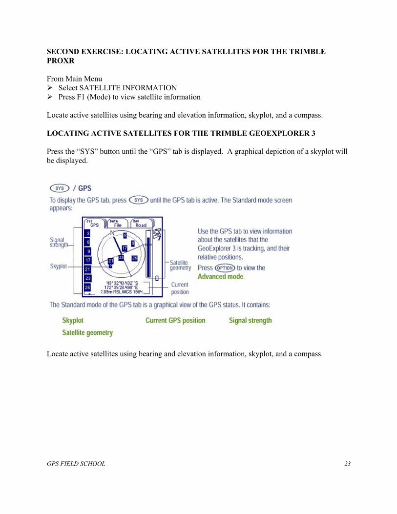
Locate active satellites using bearing and elevation information, skyplot, and a compass. LOCATING ACTIVE SATELLITES FOR THE TRIMBLE GEOEXPLORER 3 Press the “SYS” button until the “GPS” tab is displayed. A graphical depiction of a skyplot will be displayed.

Locate active satellites using bearing and elevation information, skyplot, and a compass. GPS FIELD SCHOOL 23

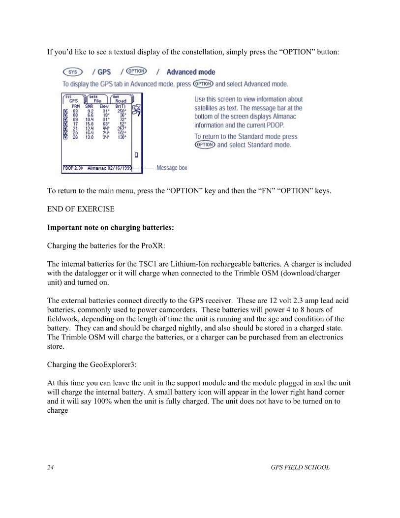
If you’d like to see a textual display of the constellation, simply press the “OPTION” button:

To return to the main menu, press the “OPTION” key and then the “FN” “OPTION” keys. END OF EXERCISE Important note on charging batteries: Charging the batteries for the ProXR: The internal batteries for the TSC1 are Lithium-Ion rechargeable batteries. A charger is included with the datalogger or it will charge when connected to the Trimble OSM (download/charger unit) and turned on. The external batteries connect directly to the GPS receiver. These are 12 volt 2.3 amp lead acid batteries, commonly used to power camcorders. These batteries will power 4 to 8 hours of fieldwork, depending on the length of time the unit is running and the age and condition of the battery. They can and should be charged nightly, and also should be stored in a charged state. The Trimble OSM will charge the batteries, or a charger can be purchased from an electronics store. Charging the GeoExplorer3: At this time you can leave the unit in the support module and the module plugged in and the unit will charge the internal battery. A small battery icon will appear in the lower right hand corner and it will say 100% when the unit is fully charged. The unit does not have to be turned on to charge

24 GPS FIELD SCHOOL

NOTES

GPS FIELD SCHOOL 25

Session 3: INTRODUCTION TO DATA COLLECTION THIRD EXERCISE: PRACTICING DATA CAPTURE WITH THE TRIMBLE PROXR NOTE: The antenna is the point that is recorded, always be aware of where the antenna is!

From Main Menu, highlight and select DATA COLLECTION Select CREATE NEW FILE Start typing to name file

File naming convention A0921F01 Team Letter = A Month and Day = 0921 (September 21) File Number = F01

Press Enter to set file name and move to Data Dictionary option Press right arrow for list of data dictionaries, highlight and select “Generic” Check Free space for file storage, should be greater than 250 KB for a day's work

(If there is not enough space, press ESC to return to the FILE MANAGER menu, then select Delete File(s))

Press ENTER to continue. The generic data dictionary is now displayed. It lets you capture data in three ways:

Point (collected positions are averaged as a point) Line (maps a line as you walk it) Area (defines a polygon as you walk around it)

Soft keys are keys that change function depending on which menu you are using. The function is shown on the bottom of the display screen. Each function corresponds with the Function button below it on the keyboard. For instance, the F3 button is REPEAT when in data capture and not logging, but NEST when logging a line. In this screen:

F1 PAUSE allows the user to pause data collection. We have set our dataloggers to collect information only when a feature is active. When in this screen, no feature is active, therefore there is no need to use pause at this time.

F2 REVIEW Lets you review the features that you have already collected in that file. F3 REPEAT lets you repeat a feature of the type that is highlighted. If “point-

generic” is highlighted, a new point will start logging. All attributes will be filled in exactly as they were for the last point-generic, but can be edited.

F4 QUICK allows you to log a point with a single position. F5 EXT allows you to check status of external sensors (N/A)

To log a point feature

Stand on or as close as possible to feature and remain stationary until all positions (10 minimum) are collected and the feature is ended (ENTER) or PAUSED (F1).

Highlight Point (generic) and press Enter to begin logging View soft keys at bottom of the screen. • F1 PAUSE allows you to pause data collection, press F1 again to resume.

26 GPS FIELD SCHOOL

• F2 REVIEW Lets you review the features that you have already collected in that file. • F3 EXT allows you to check status of external sensors (N/A) • F4 OFFSET allows you to stand away from the point and record it.

Press ENTER to end logging feature and return to data dictionary To use an offset to record a point While recording a point feature press F3 OFFSET. Make sure the format (soft key F2) is bearing/horizontal distance/vertical distance. Bearing In degrees from you to the feature Horizontal Distance from you to the feature (if you type in a distance in units other

than what you indicated in the configuration the TSC1 will do a conversion)

Vertical Distance You only need to worry about this if you are recording elevation

Press enter and this will return you to the feature you are recording. You can add an offset at any before you end the feature. To log a line feature

Highlight Line (generic) and press enter to begin logging. Walk briskly and use PAUSE (F1) if you need to stop.

View soft keys at bottom of the screen. • F1 PAUSE or RESUME • F2 REVIEW Lets you review the features that you have already collected in that file. • F3 NEST allows you to temporarily stop logging positions to your line feature and

log a point instead. This is discussed further below • F4 SEG lets you segment your line feature. This is used when the attributes of a line

feature change. This is discussed further below. • F5 (arrow) allows you to access additional soft keys • (F5) F1 EXT allows you to check status of external sensors (N/A). • (F5) F2 OFFSET allows you to record the line from a distance. (Think of soft keys as asking you a question—‘Do you want to Pause?’, etc.)

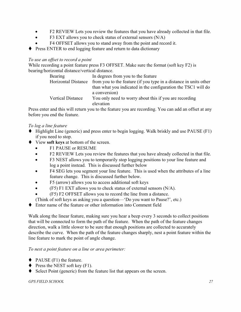
Enter name of the feature or other information into Comment field Walk along the linear feature, making sure you hear a beep every 3 seconds to collect positions that will be connected to form the path of the feature. When the path of the feature changes direction, walk a little slower to be sure that enough positions are collected to accurately describe the curve. When the path of the feature changes sharply, nest a point feature within the line feature to mark the point of angle change. To nest a point feature on a line or area perimeter:

PAUSE (F1) the feature. Press the NEST soft key (F1). Select Point (generic) from the feature list that appears on the screen.

GPS FIELD SCHOOL 27

RESUME (F1). Enter a comment, i.e. "angle point"

When sufficient positions have been collected, press OK to close the point feature. RESUME (F1) Continue to walk along the linear feature. Press ENTER to record the line feature.

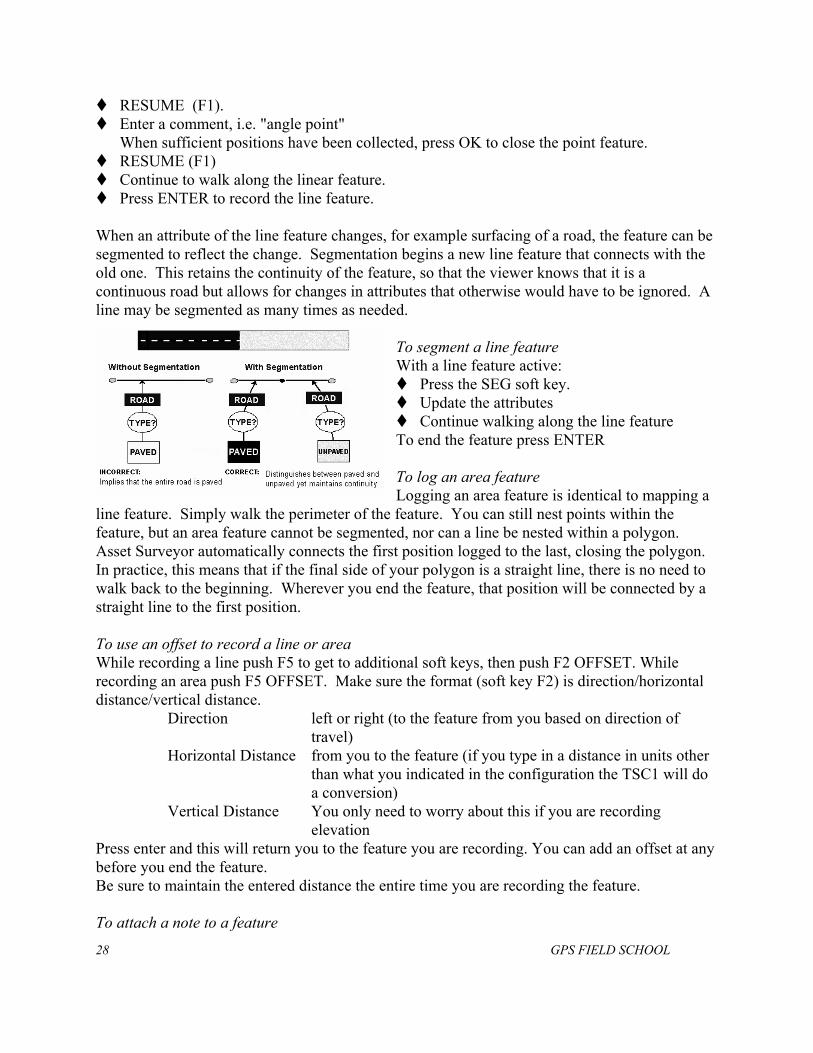
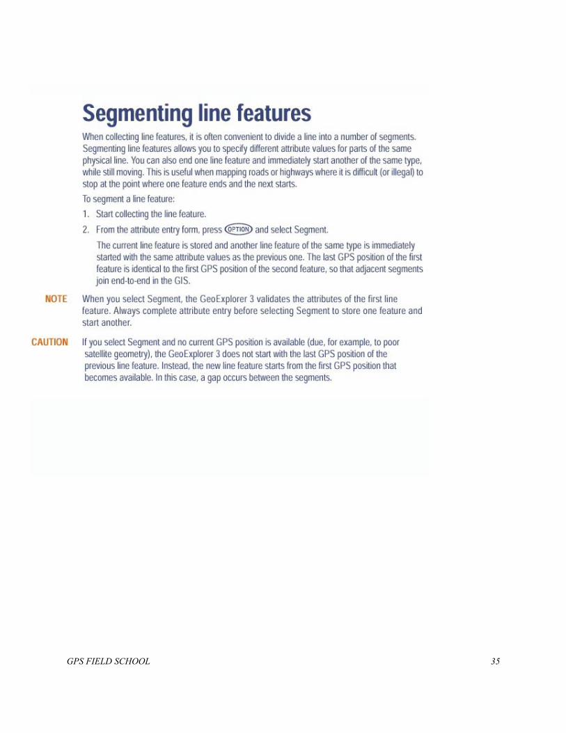
When an attribute of the line feature changes, for example surfacing of a road, the feature can be segmented to reflect the change. Segmentation begins a new line feature that connects with the old one. This retains the continuity of the feature, so that the viewer knows that it is a continuous road but allows for changes in attributes that otherwise would have to be ignored. A line may be segmented as many times as needed.

To segment a line feature With a line feature active:

Press the SEG soft key. Update the attributes Continue walking along the line feature

To end the feature press ENTER To log an area feature Logging an area feature is identical to mapping a

line feature. Simply walk the perimeter of the feature. You can still nest points within the feature, but an area feature cannot be segmented, nor can a line be nested within a polygon. Asset Surveyor automatically connects the first position logged to the last, closing the polygon. In practice, this means that if the final side of your polygon is a straight line, there is no need to walk back to the beginning. Wherever you end the feature, that position will be connected by a straight line to the first position. To use an offset to record a line or area While recording a line push F5 to get to additional soft keys, then push F2 OFFSET. While recording an area push F5 OFFSET. Make sure the format (soft key F2) is direction/horizontal distance/vertical distance. Direction left or right (to the feature from you based on direction of

travel) Horizontal Distance from you to the feature (if you type in a distance in units other

than what you indicated in the configuration the TSC1 will do a conversion)

Vertical Distance You only need to worry about this if you are recording elevation

Press enter and this will return you to the feature you are recording. You can add an offset at any before you end the feature. Be sure to maintain the entered distance the entire time you are recording the feature. To attach a note to a feature

28 GPS FIELD SCHOOL

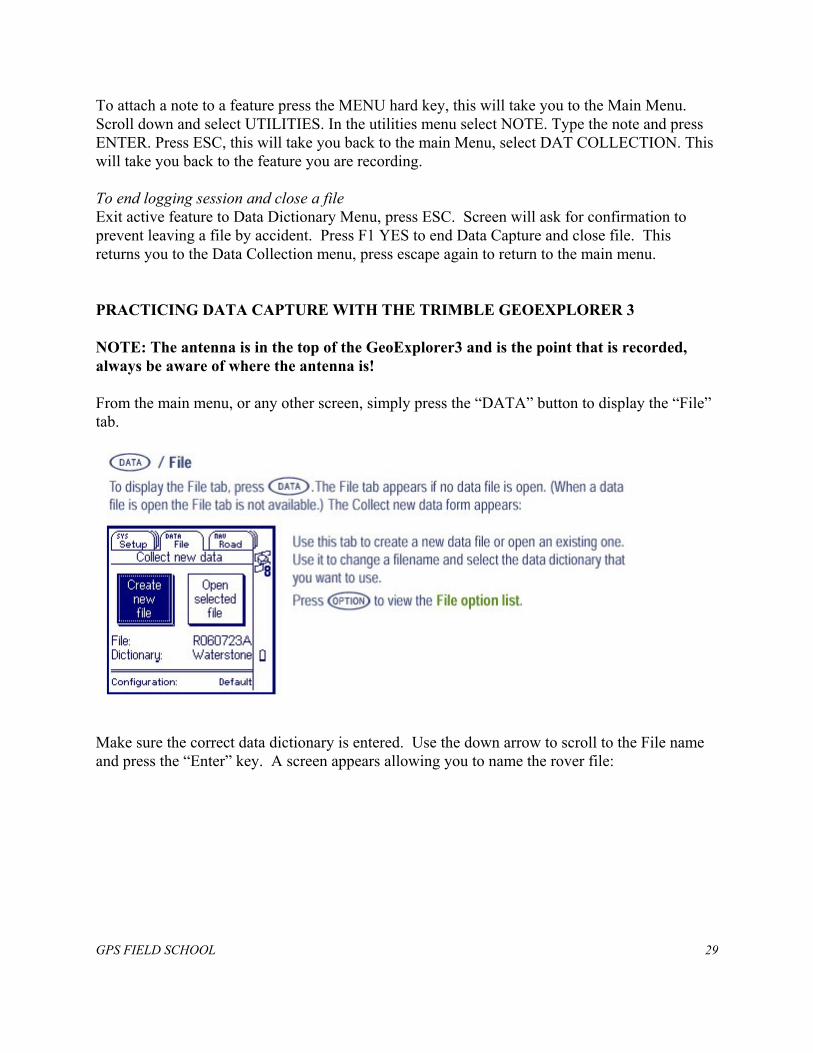
To attach a note to a feature press the MENU hard key, this will take you to the Main Menu. Scroll down and select UTILITIES. In the utilities menu select NOTE. Type the note and press ENTER. Press ESC, this will take you back to the main Menu, select DAT COLLECTION. This will take you back to the feature you are recording. To end logging session and close a file Exit active feature to Data Dictionary Menu, press ESC. Screen will ask for confirmation to prevent leaving a file by accident. Press F1 YES to end Data Capture and close file. This returns you to the Data Collection menu, press escape again to return to the main menu. PRACTICING DATA CAPTURE WITH THE TRIMBLE GEOEXPLORER 3 NOTE: The antenna is in the top of the GeoExplorer3 and is the point that is recorded, always be aware of where the antenna is! From the main menu, or any other screen, simply press the “DATA” button to display the “File” tab.

Make sure the correct data dictionary is entered. Use the down arrow to scroll to the File name and press the “Enter” key. A screen appears allowing you to name the rover file:

GPS FIELD SCHOOL 29

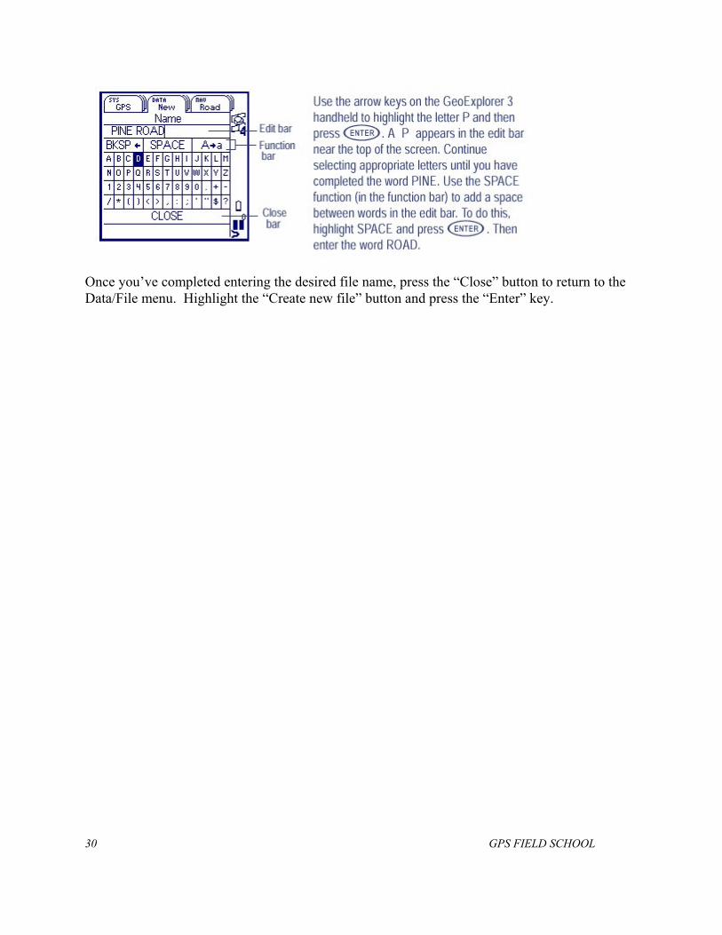
Once you’ve completed entering the desired file name, press the “Close” button to return to the Data/File menu. Highlight the “Create new file” button and press the “Enter” key.

30 GPS FIELD SCHOOL

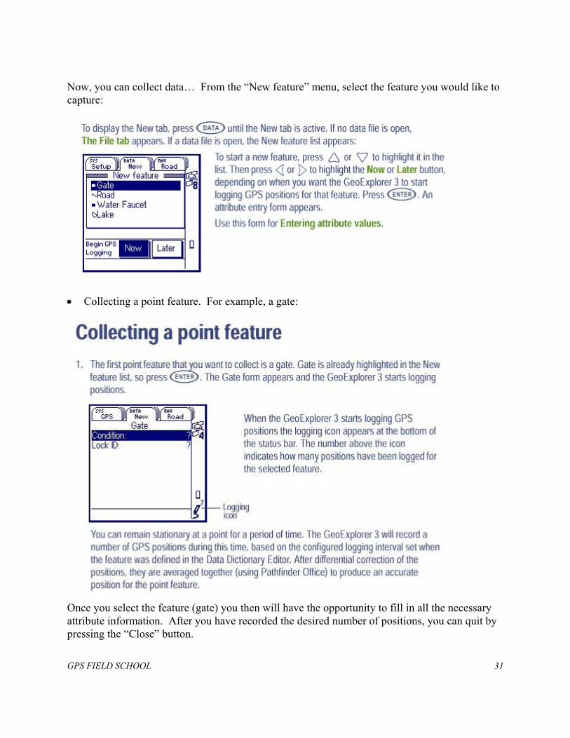
Now, you can collect data… From the “New feature” menu, select the feature you would like to capture:

• Collecting a point feature. For example, a gate:

Once you select the feature (gate) you then will have the opportunity to fill in all the necessary attribute information. After you have recorded the desired number of positions, you can quit by pressing the “Close” button.

GPS FIELD SCHOOL 31

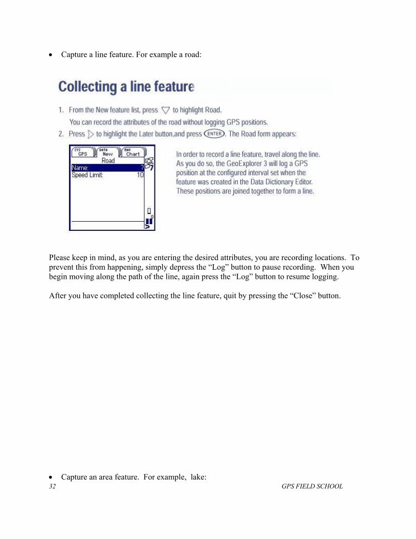
• Capture a line feature. For example a road:

Please keep in mind, as you are entering the desired attributes, you are recording locations. To prevent this from happening, simply depress the “Log” button to pause recording. When you begin moving along the path of the line, again press the “Log” button to resume logging. After you have completed collecting the line feature, quit by pressing the “Close” button.

32 GPS FIELD SCHOOL • Capture an area feature. For example, lake:

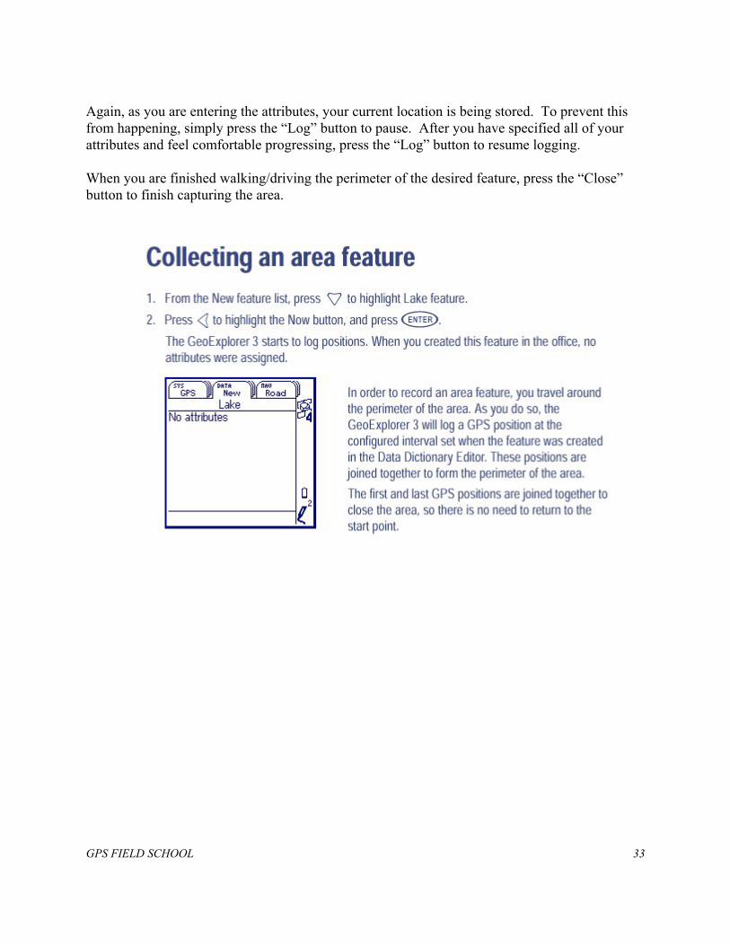
Again, as you are entering the attributes, your current location is being stored. To prevent this from happening, simply press the “Log” button to pause. After you have specified all of your attributes and feel comfortable progressing, press the “Log” button to resume logging. When you are finished walking/driving the perimeter of the desired feature, press the “Close” button to finish capturing the area.

GPS FIELD SCHOOL 33

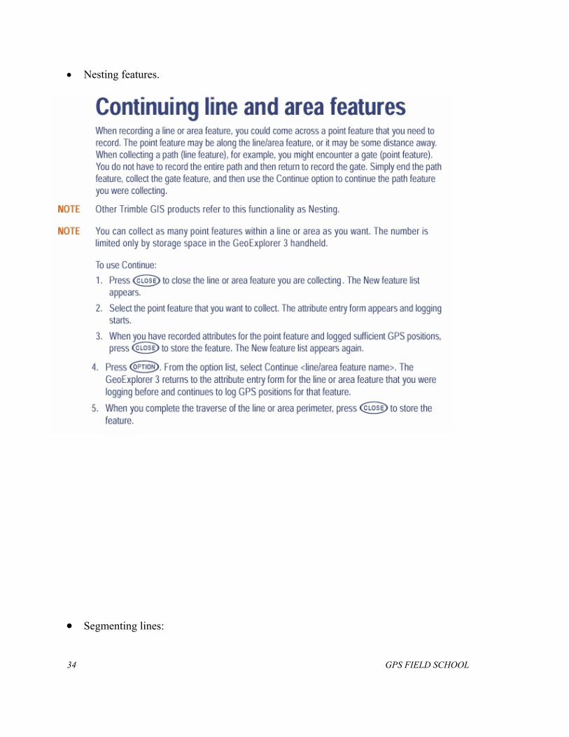
• Nesting features.

• Segmenting lines:

34 GPS FIELD SCHOOL

GPS FIELD SCHOOL 35

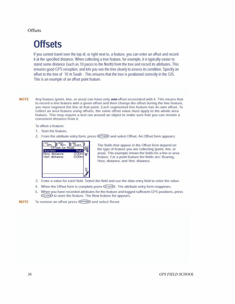
Offsets

36 GPS FIELD SCHOOL

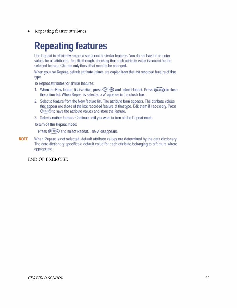
Repeating feature attributes: •

END OF EXERCISE

GPS FIELD SCHOOL 37

NOTES

38 GPS FIELD SCHOOL

Session 4: INTRODUCTION TO PATHFINDER OFFICE Pathfinder Office is the PC end of the data collection software you have already seen. The data you collect using an MC-V is downloaded to the PC via the 9 pin to 9 pin null-modem cable that is included with the hardware. From the TDC-1, a specialized round 12 pin to 9 pin cable is used. This is also included with the hardware. FOURTH EXERCISE: EXPLORING PATHFINDER OFFICE In this exercise we will configure the Pathfinder Office program to look the way we want, download data from the datalogger to the PC, and look at our data on screen as lines, points, and areas. Pathfinder Office is mouse and menu driven, like any Windows compatible program. Use the left mouse button unless otherwise instructed. Also, the menus can be accessed by the use of "hot keys" These keystrokes are a combination of the ALT key and a standard key. The hot key will be underlined on the menu button on screen. So for example, to quit Pathfinder Office program, you can either click FILE EXIT or type ALT-F (to access the file menu) then ALT-X .

To start the program, double click the Pathfinder Office icon PROJECTS The project is the main way in which data is organized in Pathfinder Office. A project is nothing more than a directory where Pathfinder Office looks for data. Usually, a project contains data associated with one geographic location or perhaps one type of resource (for example, a cultural resources project and a natural resources project). Data files are stored in the project directory, and there are three subdirectories in a project for organizing other kinds of files: base, export and backup. The backup subdirectory contains backup copies of field collected files. When data is downloaded from the datalogger, an extra copy of each file is placed in this subdirectory. The base subdirectory is where you should store base station files for differential correction. These files will be discussed in a later session. The export subdirectory is the default target location when GPS files are exported for use in another program. This is also covered in a later session. NOTE: Do not rename or delete any of the default folders in the project folder or Pathfinder Office will not open the project.

GPS FIELD SCHOOL 39

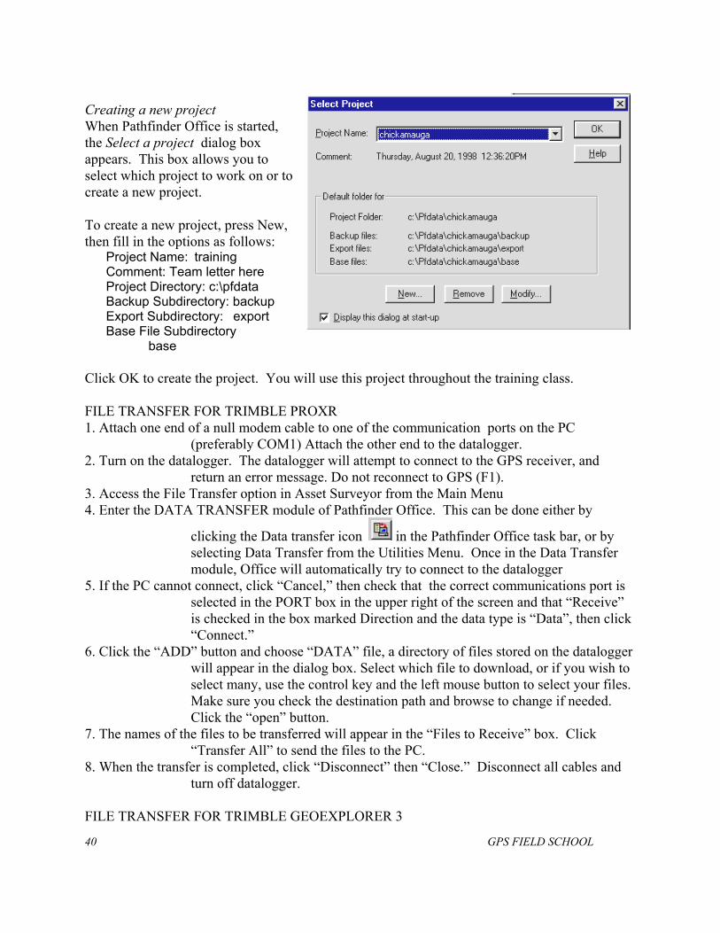
Creating a new project When Pathfinder Office is started, the Select a project dialog box appears. This box allows you to select which project to work on or to create a new project. To create a new project, press New, then fill in the options as follows:

Project Name: training Comment: Team letter here Project Directory: c:\pfdata Backup Subdirectory: backup Export Subdirectory: export Base File Subdirectory base

Click OK to create the project. You will use this project throughout the training class. FILE TRANSFER FOR TRIMBLE PROXR 1. Attach one end of a null modem cable to one of the communication ports on the PC

(preferably COM1) Attach the other end to the datalogger. 2. Turn on the datalogger. The datalogger will attempt to connect to the GPS receiver, and

return an error message. Do not reconnect to GPS (F1). 3. Access the File Transfer option in Asset Surveyor from the Main Menu 4. Enter the DATA TRANSFER module of Pathfinder Office. This can be done either by

clicking the Data transfer icon in the Pathfinder Office task bar, or by selecting Data Transfer from the Utilities Menu. Once in the Data Transfer module, Office will automatically try to connect to the datalogger

5. If the PC cannot connect, click “Cancel,” then check that the correct communications port is selected in the PORT box in the upper right of the screen and that “Receive” is checked in the box marked Direction and the data type is “Data”, then click “Connect.”

6. Click the “ADD” button and choose “DATA” file, a directory of files stored on the datalogger will appear in the dialog box. Select which file to download, or if you wish to select many, use the control key and the left mouse button to select your files. Make sure you check the destination path and browse to change if needed.

Click the “open” button. 7. The names of the files to be transferred will appear in the “Files to Receive” box. Click

“Transfer All” to send the files to the PC. 8. When the transfer is completed, click “Disconnect” then “Close.” Disconnect all cables and

turn off datalogger. FILE TRANSFER FOR TRIMBLE GEOEXPLORER 3

40 GPS FIELD SCHOOL

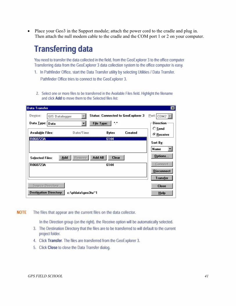
• Place your Geo3 in the Support module; attach the power cord to the cradle and plug in. Then attach the null modem cable to the cradle and the COM port 1 or 2 on your computer.

GPS FIELD SCHOOL 41

DISPLAY THE DATA Pathfinder Office will open with three windows. The first, the MAP window is the graphic display of the data as points, lines and areas. If this display does not appear it can be opened from the menu : View—>Map. The second, POSITION PROPERTIES, displays coordinate information and is used for editing, which is covered in a later session. The last window is the FEATURE PROPERTIES and it displays all the information on the highlighted feature: this box will also be used for editing. The QUERY POSITION and FEATURE PROPERTIES displays can also be opened from the menu: Data—>Feature Properties or Data—>Position Properties Opening a data file Pathfinder Office can display many files at once. However, you can only open one file at a time if you wish to edit the file. In the Files menu, select open. Type the name of the file to be displayed or select from the directory listing using the mouse. To select a block of sequential files from the directory, select the first file in the block, then press shift and click on the last file. To select a non-sequential group of files, use the control key then click on the desired files. When all desired files are highlighted, press Open. Options The options menu allows you to specify the units and projection system of the display. Although the GPS data is collected on the datalogger in latitude longitude coordinates, it can be displayed in a number of other systems, such as Universal Transverse Mercator (UTM) or State Plane system. Background files In order to make editing easier, Pathfinder Office can display geographic data in many different file formats as background. This allows you to open a single file for editing, but still see the features in context. Images can also be displayed as background files. There are additional considerations for using an image, however. Image data cannot be transformed by Pathfinder Office into a new projection system. The image must be registered to the current projection system in order to display. If you wish to display an image, change the current projection system under the options menu. To load a background file to the map window, select Files --> Background and press the

button. Select the desired file from the directory list. You can select Trimble files, as well as DXF (Autocad format), SHP (ArcView format), TIF (TIFF images) among others. The box entitled “List Files of Type:” allows you to specify which types of files will be displayed in the directory listing. You can also maneuver throughout the directory system to find specific files elsewhere on the hard drive or on a floppy disk.

Once a file is in the Background files list, use the button to block it from display,

to add it back to the display and to remove the file name from the list altogether. A check mark next to the file name indicates that it will be displayed. NOTE: You should not display the file that is open for editing. This will cause confusion,

42 GPS FIELD SCHOOL

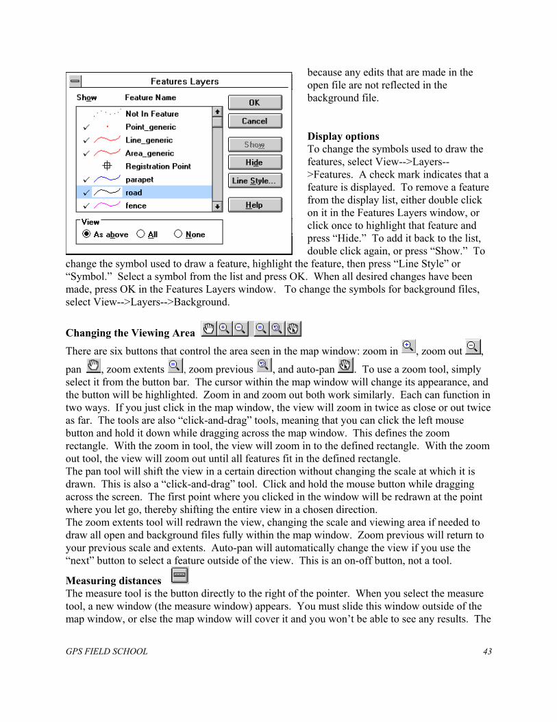
because any edits that are made in the open file are not reflected in the background file. Display options To change the symbols used to draw the features, select View-->Layers-->Features. A check mark indicates that a feature is displayed. To remove a feature from the display list, either double click on it in the Features Layers window, or click once to highlight that feature and press “Hide.” To add it back to the list, double click again, or press “Show.” To

change the symbol used to draw a feature, highlight the feature, then press “Line Style” or “Symbol.” Select a symbol from the list and press OK. When all desired changes have been made, press OK in the Features Layers window. To change the symbols for background files, select View-->Layers-->Background.

Changing the Viewing Area

There are six buttons that control the area seen in the map window: zoom in , zoom out ,

pan , zoom extents , zoom previous , and auto-pan . To use a zoom tool, simply select it from the button bar. The cursor within the map window will change its appearance, and the button will be highlighted. Zoom in and zoom out both work similarly. Each can function in two ways. If you just click in the map window, the view will zoom in twice as close or out twice as far. The tools are also “click-and-drag” tools, meaning that you can click the left mouse button and hold it down while dragging across the map window. This defines the zoom rectangle. With the zoom in tool, the view will zoom in to the defined rectangle. With the zoom out tool, the view will zoom out until all features fit in the defined rectangle. The pan tool will shift the view in a certain direction without changing the scale at which it is drawn. This is also a “click-and-drag” tool. Click and hold the mouse button while dragging across the screen. The first point where you clicked in the window will be redrawn at the point where you let go, thereby shifting the entire view in a chosen direction. The zoom extents tool will redrawn the view, changing the scale and viewing area if needed to draw all open and background files fully within the map window. Zoom previous will return to your previous scale and extents. Auto-pan will automatically change the view if you use the “next” button to select a feature outside of the view. This is an on-off button, not a tool.

Measuring distances The measure tool is the button directly to the right of the pointer. When you select the measure tool, a new window (the measure window) appears. You must slide this window outside of the map window, or else the map window will cover it and you won’t be able to see any results. The

GPS FIELD SCHOOL 43

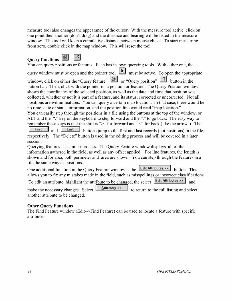
measure tool also changes the appearance of the cursor. With the measure tool active, click on one point then another (don’t drag) and the distance and bearing will be listed in the measure window. The tool will keep a cumulative distance between mouse clicks. To start measuring from zero, double click in the map window. This will reset the tool.

Query functions You can query positions or features. Each has its own querying tools. With either one, the

query window must be open and the pointer tool must be active. To open the appropriate

window, click on either the “Query feature” or “Query position” button in the button bar. Then, click with the pointer on a position or feature. The Query Position window shows the coordinates of the selected position, as well as the date and time that position was collected, whether or not it is part of a feature, and its status, corrected or uncorrected. Not all positions are within features. You can query a certain map location. In that case, there would be no time, date or status information, and the position line would read “map location.” You can easily step through the positions in a file using the buttons at the top of the window, or ALT and the “.” key on the keyboard to step forward and the “,” to go back. The easy way to remember these keys is that the shift is “>“ for forward and “<“ for back (like the arrows). The

and buttons jump to the first and last records (not positions) in the file, respectively. The “Delete” button is used in the editing process and will be covered in a later session. Querying features is a similar process. The Query Feature window displays all of the information gathered in the field, as well as any offset applied. For line features, the length is shown and for area, both perimeter and area are shown. You can step through the features in a file the same way as positions. One additional function in the Query Feature window is the button. This allows you to fix any mistakes made in the field, such as misspellings or incorrect classifications. To edit an attribute, highlight the attribute to be changed, the select and

make the necessary changes. Select to return to the full listing and select another attribute to be changed. Other Query Functions The Find Feature window (Edit-->Find Feature) can be used to locate a feature with specific attributes.

44 GPS FIELD SCHOOL

NOTES

GPS FIELD SCHOOL 45

Session 5: PROJECT DEVELOPMENT AND DATA DICTIONARY DESIGN The real world is a complicated place, full of innumerable features (things) with innumerable attributes (sizes, colors, shapes, types). We cannot map everything in the real world; therefore, we simplify the real world into something we can handle. Some real world variables are useful for understanding relationships between the parts and the whole, for orienting ourselves in space and time, or for answering research questions and generating statistics; other variables are incidental or superfluous to the task at hand. To simplify, we select those features and attributes that we wish to observe and ignore the rest. We isolate features of interest and filter out extraneous noise. This selection process results in a simplified “model” of reality that can be more easily manipulated, analyzed, and translated into a map. We cannot map everything in the real world; therefore, we construct a model of reality, called a “cartographic model,” to guide our GPS survey in the field. A cartographic model consists of specific features and attributes selected from the real world and organized in a way that makes apparent the relationships between these features within a landscape. Selection of features and attributes is based on interest and need. From our cartographic model we can derive a list of essential features and attributes that we wish to observe in the field. This list becomes our project data dictionary. The data dictionary becomes the surveyors’ eyes in the field. It directs the surveyors to observe what we want them to see and to filter out the rest. When selecting those features and attributes in the real world that we wish surveyors to observe, it is important not to leave something out of the data dictionary that is essential to the purpose of the survey. For example, if the task at hand is to map an historic landscape, all of the major features that define the landscape (road traces, woodlots, house sites, fence lines, etc.) should be included in the data dictionary. If major features are omitted, the surveyor probably will not map those features or else will record them sporadically. The data collected in the field will be incomplete and disorganized. Once data has been observed in the field, recorded in GPS, and loaded into the computer it can be related to other layers of information through the use of Geographic Information Systems. This is where the results of the GPS survey are displayed in relationship to other map layers and where the data can be used to generate statistics, measure distances and areas, develop new cartographic models, propose new sets of research questions, and design and print hard copy maps. Thus, we move from the real world to a model that contains selected elements of the real world. From this model we develop the data dictionary that guides the GPS surveyor through the landscape. This results in data layers in the digital world. Once in GIS, the information can be used to influence decisions that, in turn, have an impact on reality. For example, by overlaying in GIS a proposed residential development upon historic landscape features recorded with GPS, we could measure and display the impact of the development on the historic resources. This, in turn, might result in a plan to preserve some of the resources. Or, if we were to map the locations of vegetation types, we would know where to focus our efforts to combat plant disease or insect infestation. If we were to map metal utility poles and interpretive signs and noted their condition, we would know where to spend next year’s paint budget. 46 GPS FIELD SCHOOL

A well-conceived data dictionary--one that simplifies reality yet does not exclude anything essential--is the key to a successful GPS survey. If our analyses are flawed by incomplete or inaccurate information, subsequent actions taken in the real world will equally be flawed. By thinking carefully about a project before going into the field, we can avoid the dreaded words, “garbage in... garbage out.” Project Design There are four major steps in project planning and design:

1) Decide on the purpose of the survey 2) Write a project description and outline the project’s research questions 3) Decide on the level of accuracy needed for mapping and analysis 4) Determine which data layers must be created, and which are already available

1) Decide on the purpose of the survey A GPS survey can be conducted for three major purposes:

to build a baseline inventory of resource information to answer questions about those resources for a specific application. to implement some combination of these

A baseline inventory survey is designed to capture data for the purpose of gaining an overview of the resource base. Although it may have no immediate specific application, a baseline inventory serves as an all-purpose database that can be used in future GIS analyses. The baseline inventory provides a context for all specific applications. In developing a data dictionary for baseline inventory, it is important to know what data is already available, to organize what needs to be mapped by resource types (cultural, natural, maintenance, interpretation, etc.) and to prioritize the features to be mapped (you cannot map everything at once). A baseline inventory survey tends to be “feature-oriented,” containing many features but fewer attributes for each feature. In developing a data dictionary for a specific application survey, it is important to identify a problem, define questions that will help solve the problem, and identify the data needed to answer these questions. The project leader must determine how the spatial data will be manipulated to yield a result or “solution.” In practice, one begins by visualizing a solution and working backwards to define the kinds of spatial data needed to “map” the solution. For example, campers and hikers are threatened by dead trees and falling limbs. Maintenance of hazard trees is a daily concern in parks. Knowing the location of all of the hazardous trees around the camping areas and along the trails would enable the maintenance crew to budget time and money for posting, topping, or removal. Knowing the type and size of the tree, or assigning a “hazard level” of very high, high, and moderate, would enable the tree crew to focus on problem areas and make most efficient use of time and money. A survey for a specific application tends to be “attribute-oriented,” containing fewer features but collecting more in-

GPS FIELD SCHOOL 47

depth descriptions of each. Sometimes the baseline inventory needs to be expanded before more specific research questions can be answered, resulting in a combined approach that builds the inventory while attempting to answer a specific question. A combined survey attempts to balance the breadth of features covered with the depth of attributes captured. In such circumstances, the project leader can create one data dictionary that contains many inventory features but requires more in-depth description for one or two specific features. 2) Write a Project Description and Outline Research Questions A project description briefly explains the purpose of the project, the research questions that are to be answered, the methodology to be used, the number of persons available for the survey, the amount of time allotted for the survey, and the desired end product. It is important to determine whether the purpose of the project is to build a baseline inventory, to develop solutions for a specific application, or to combine the two approaches. Make a list of research questions that you wish to answer. These may be as broad as “how many miles of hiking trails are in the park?” or as focused as “In which areas do the oak trees show signs of disease and decay?” The research questions will be used to determine the breadth of features and depth of attributes in the data dictionary. The availability of staff, equipment, and time will influence how the survey will be conducted--whether it will focus on a narrow geographic area or attempt to cover a lot of ground. How many people and GPS units are available? Is this a multi-team operation or a one-person show? Should teams work together mapping different features in the same geographic area or divide the landscape into sectors? How much time is available? Will this be a comprehensive effort or a quick once-over? Are the surveyors knowledgeable about the subject matter? Will they be able to identify the attributes? In the above example regarding diseased oak trees, the surveyors must be able to recognize an oak tree as well as the signs of disease and decay in order to fill in the correct attribute values. When developing a data dictionary, it is important to visualize an end product. What is the final product? Will the survey result in new layers for the computer database? Will the GPS data be used to print out paper maps for inclusion in a report? Will the attribute information be used to generate statistics? The end product may influence the types of information collected, the scope of the survey, the scale and level of accuracy.

48 GPS FIELD SCHOOL

3) Decide on the level of accuracy needed for mapping and analysis The purpose of the survey and the required scale of the finished product will influence the level of accuracy that is required. Baseline inventory data should be collected at a scale that is comparable to existing resource base maps. This will vary by organization, location, or park. It makes little sense to collect highly accurate data for your baseline inventory if it is going to be used to augment small-scale 1:250,000 maps. There are easier ways to get this kind of information into the computer. On the other hand, most site plans and tax parcel maps are produced at a scale of 1:2000. This scale requires the kind of detailed information that can be collected efficiently by GPS. Data collected for a specific application needs to be detailed enough to resolve the analysis, which in most cases needs to be very detailed indeed. Below are some of the standard levels of mapping accuracy:

* 1:250,000 scale USGS 1 x 2-degree series ± 250 meters * 1:100,000 scale USGS 30 x 60-minute series ± 90 meters * 1:24,000 scale USGS 7.5-minute quadrangle maps ± 12 meters * 1:2000 scale site plans and tax parcel maps ± 5 meters (varies widely) * GPS (mapping grade) ± 1 meter * GPS (survey grade) ±10 centimeters * Laser transit boundary line survey ± 5 centimeters

4) Determine what information is needed and what information is already available Think about the finished product outlined in your project description. What information do you need to complete that product? If your survey is an inventory, the information needed is just what is described in step 2. If your project is a specific application, you may need to compare different data sets to arrive at the final product. Determine which layers of information are already available in your database or from other sources. Other sources could mean purchasing digital data from USGS or other GIS agencies, digitizing data from USGS quad sheets, or importing existing dBASE or other databases. Often, there is an easier way to get the information into the computer than by deploying a GPS survey. Is this data of sufficient accuracy to provide a context for specific applications? A GPS survey should be used to capture details that are unavailable from standard map sources. For instance, to use GIS to site a hiking trail, you need to know slope, soil type and the locations of the resources you wish to include in this hiking tour. Slope and soil type are available from the USGS and the SCS respectively. The resources to be included on the tour will not be readily available from any other source, and are the prime target of a GPS survey. Examine existing documentation, such as surveys, reports, maps, or databases, for ideas on how to organize data collection and design your data dictionary.

GPS FIELD SCHOOL 49

Developing Your Data Dictionary There are three major steps for developing a good data dictionary:

1) Identify features to be observed and mapped 2) Identify attributes that will be recorded for each feature 3) Test the data dictionary to ensure that nothing essential is left out

1) Identify features to map There are two types of features to map in any given GPS survey:

Target features (those required to complete the inventory or application) Reference features (those required to provide context)

Target features are those needed to augment the existing inventory or to answer specific questions. Reference features serve as a check on the location of the target features and provide a frame of reference for defining the boundaries of the project area. For example, although the primary target feature may be the boundary of an endangered species’ habitat, it would be essential to map the road network surrounding the area, trails leading into the habitat, nearby structures, and so forth, so that the finished map layers can be used to guide a biologist back to the site in the future. Reference features also serve the purpose of assisting in editing linear data. Take for example, a project that requires an inventory of historic walls. If a wall runs alongside a hiking trail, it would be very helpful to map the hiking trail as well, so that you can be assured of the accuracy of your data and also be able to edit the linear features properly (See Session 9). Another example of reference features that are useful to include in any data dictionary are “line points.” These are point features that are taken at the beginning, end and angle points of a line feature. Line points are very helpful in editing line features, because they allow you to use a “connect the dots” approach. Point features are the most accurate data you will collect. With line points in your data dictionary, you can utilize the accuracy of point features to anchor lines and polygons. In the real world every feature has an area; but in the digital world we simplify:

Very small areas become points. Long, skinny areas are symbolized as lines. Larger areas remain as polygons.

The decision to collect point, line, or polygon data will depend on the scale at which the data will be used and displayed, the type of statistics you wish to generate for each feature, and the accuracy of the equipment. How are resources typically symbolized on your baseline inventory database? You should maintain the following conventions:

If surface area is needed then features must be mapped as polygons If only length is required then features can be lines

50 GPS FIELD SCHOOL

If only location is desired then features can be points Another consideration is the resolution of the survey instrument. For example, the Trimble ProXL with an 8-channel receiver delivers an accuracy of ± 1-meter, 90% of the time; therefore areas under 2 X 2 meters should be mapped only as points. 2) Identify attributes that will be recorded for each feature In moving from the real world to the digital world we must simplify:

Make a limited number of essential observations Describe features so that they are easily recognizable in the field

For an inventory project:

What attributes are most often used to describe the feature; e.g. site condition? What attributes will allow linkage to other databases; e.g. identification number?

For a specific application project:

What characteristics are used in the analysis? Other considerations:

Editing functions; i.e. begin point, end point, angle point Links from the digital world to the real world, or to other digital sources How the attribute information will be used or queried

Attribute values can be collected in seven different formats; each suited to a particular purpose.

Menu: user chooses from a predefined list of options Numeric: distinct numeric values, such as counts of resources or heights Text: user enters up to 100 characters of text Date: automatically enters current date Time: automatically enters current time File Name: automatically enters file name

Menu attributes:

standardize selections constrain choices reduce errors make it easier to query

however: not as flexible as character fields must be well thought out before going into the field

GPS FIELD SCHOOL 51

Character and numeric attributes: open ended very flexible can respond to unanticipated field conditions

however: are difficult to query increase the chance of typographical errors results often in non-standardized choices

Sometimes a feature has no attributes. For certain features, no information is needed beyond the location. Also, features mapped for editing reference, such as line points, might not be transferred to the GIS, and therefore do not need attributes. 3) Test the Data Dictionary You can expect to revise your data dictionary as work progresses. If at all possible, test your data dictionary under field conditions. Take it to your project site and start mapping. Look around for other features that should be in the database. Decide if additional data can be collected with minimal effort. For instance, if your project was to map an interpretive hiking trail, it will cost little additional effort to map the signs as you map the trail. A comprehensive inventory of interpretive signs can be a large undertaking, and this extra effort could give you a head start. Also test your attribute information and make sure that nothing was left out. A menu choice called “other” is often a good idea, just in case. FIFTH EXERCISE: Data Dictionary Worksheets

For this training course, project descriptions have already been prepared. Read each project description on the handout provided and propose the type of survey you would use to carry out the project. On the right side of the title of the project enter the purpose of the survey: [I] for inventory; [A] for application; [C] for a combination of both inventory and application. Discuss and identify the features that you will need to map for your assigned project. Use the sample data dictionary sheet as a guide, and on a clean worksheet:

Enter the feature name Circle its feature class Enter its first attribute name Circle its attribute type Fill in the attribute values - for menu...enter the choices - for character...enter the character limit - for numeric...enter the number of digits - for date and time...leave blank

52 GPS FIELD SCHOOL

NOTES

GPS FIELD SCHOOL 53

Session 6: ENTERING AND DOWNLOADING THE DATA DICTIONARY

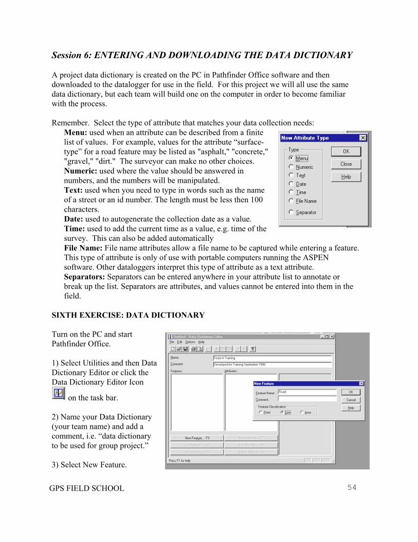
A project data dictionary is created on the PC in Pathfinder Office software and then downloaded to the datalogger for use in the field. For this project we will all use the same data dictionary, but each team will build one on the computer in order to become familiar with the process. Remember. Select the type of attribute that matches your data collection needs:

Menu: used when an attribute can be described from a finite list of values. For example, values for the attribute “surface-type” for a road feature may be listed as "asphalt," "concrete," "gravel," "dirt." The surveyor can make no other choices. Numeric: used where the value should be answered in numbers, and the numbers will be manipulated. Text: used when you need to type in words such as the name of a street or an id number. The length must be less then 100 characters. Date: used to autogenerate the collection date as a value. Time: used to add the current time as a value, e.g. time of the survey. This can also be added automatically File Name: File name attributes allow a file name to be captured while entering a feature. This type of attribute is only of use with portable computers running the ASPEN software. Other dataloggers interpret this type of attribute as a text attribute. Separators: Separators can be entered anywhere in your attribute list to annotate or break up the list. Separators are attributes, and values cannot be entered into them in the field.

SIXTH EXERCISE: DATA DICTIONARY Turn on the PC and start Pathfinder Office. 1) Select Utilities and then Data Dictionary Editor or click the Data Dictionary Editor Icon

on the task bar. 2) Name your Data Dictionary (your team name) and add a comment, i.e. “data dictionary to be used for group project.” 3) Select New Feature.

GPS FIELD SCHOOL 54

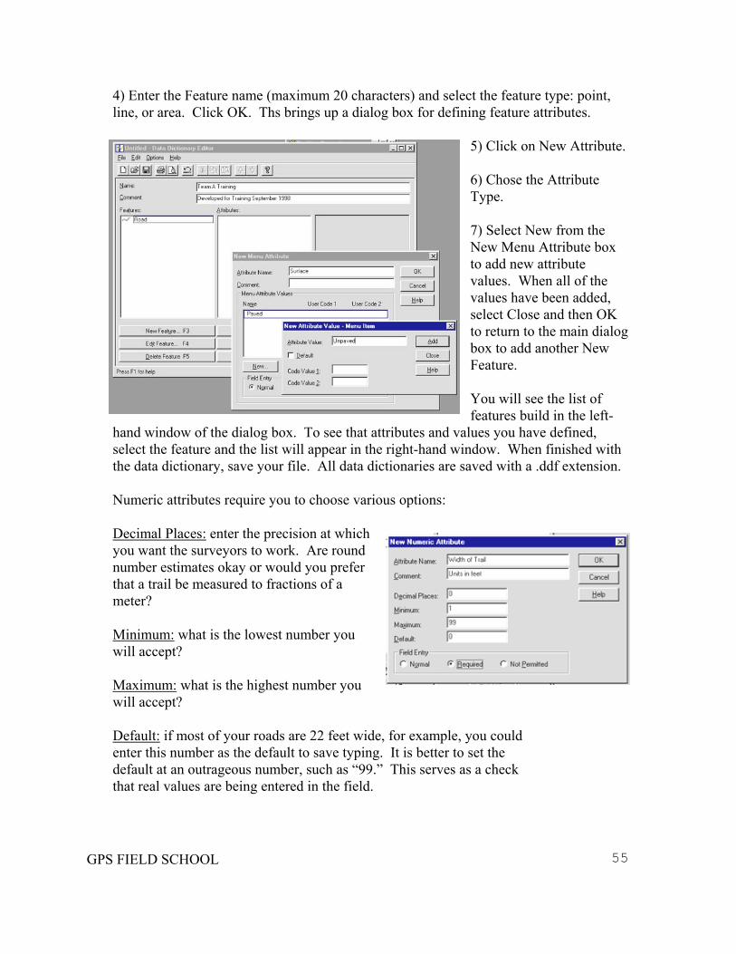
4) Enter the Feature name (maximum 20 characters) and select the feature type: point, line, or area. Click OK. Ths brings up a dialog box for defining feature attributes.

5) Click on New Attribute. 6) Chose the Attribute Type. 7) Select New from the New Menu Attribute box to add new attribute values. When all of the values have been added, select Close and then OK to return to the main dialog box to add another New Feature. You will see the list of features build in the left-

hand window of the dialog box. To see that attributes and values you have defined, select the feature and the list will appear in the right-hand window. When finished with the data dictionary, save your file. All data dictionaries are saved with a .ddf extension. Numeric attributes require you to choose various options: Decimal Places: enter the precision at which you want the surveyors to work. Are round number estimates okay or would you prefer that a trail be measured to fractions of a meter? Minimum: what is the lowest number you will accept? Maximum: what is the highest number you will accept? Default: if most of your roads are 22 feet wide, for example, you could enter this number as the default to save typing. It is better to set the default at an outrageous number, such as “99.” This serves as a check that real values are being entered in the field.

GPS FIELD SCHOOL 55

Field Entry: The Field Entry field affects the entry of values for the selected attribute while you are capturing a feature. There are three options:

Normal: value entry is optional. Use this only for attributes that are non-essential. Required: You must enter a value and cannot turn off the feature in the field until you do. This option should be selected for all essential field attributes. Not Permitted: You are not allowed to enter a value. You can use this option together with a default attribute value to prevent that value from being changed.

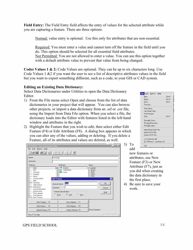
Codes Values 1 & 2: Code Values are optional. They can be up to six characters long. Use Code Values 1 &2 if you want the user to see a list of descriptive attributes values in the field but you want to export something different, such as a code, to your GIS or CAD system. Editing an Existing Data Dictionary: Select Data Dictionaries under Utilities to open the Data Dictionary Editor. 1) From the File menu select Open and choose from the list of data

dictionaries in your project that will appear. You can also browse other projects, or import a data dictionary from an .ssf or .cor file, using the Import from Data File option. When you select a file, the dictionary loads into the Editor with features listed in the left-hand window and attributes in the right.

2) Highlight the Feature that you wish to edit, then select either Edit Feature (F4) or Edit Attribute (F8). A dialog box appears in which you can alter any of the values, adding or deleting. If you delete a Feature, all of its attributes and values are deleted, as well.

3) To add new features or attributes, use New Feature (F3) or New Attribute (F7), just as you did when creating the data dictionary in the first place.

4) Be sure to save your work.

GPS FIELD SCHOOL 56

DATA DICTIONARY TRANSFER FOR TRIMBLE PROXR 1. Attach one end of a null modem cable to one of the communication ports on the PC

(preferably COM1) Attach the other end to the datalogger. 2. Turn on the datalogger. The datalogger will attempt to connect to the GPS receiver, and

return an error message. Do not reconnect to GPS (F1). 3. Access the File Transfer option in Asset Surveyor from the Main Menu 4. Enter the DATA TRANSFER module of Pathfinder Office. This can be done either by

clicking the Data transfer icon in the Pathfinder Office task bar, or by selecting Data Transfer from the Utilities Menu. Once in the Data Transfer module, Office will automatically try to connect to the datalogger

5. If the PC cannot connect, click “Cancel,” then check that the correct communications port is selected in the PORT box in the upper right of the screen and that “Send” is checked in the box marked Direction, and the file type is “Data Dictionary” then click “Connect.”

6. A list of data dictionary files in the project folder will appear in the “Available files” box. Select which one file to download, or if you wish to select many, use the control key and the left mouse button to select your files. If all files are to be downloaded, click the “Add All” button.

6. Click the “ADD” button and choose “DATA” file, a list of data dictionary files in the project folder will appear in the dialog box. Select which file to download, or if you wish to select many, use the control key and the left mouse button to select your files. Click the “open” button.

7. The names of the files to be transferred will appear in the “Files to Send” box. Click “Transfer All” to send the files to the datalogger.

8. When the transfer is completed, click “Disconnect” then “Close.” Disconnect all cables and turn off datalogger.

GPS FIELD SCHOOL 57

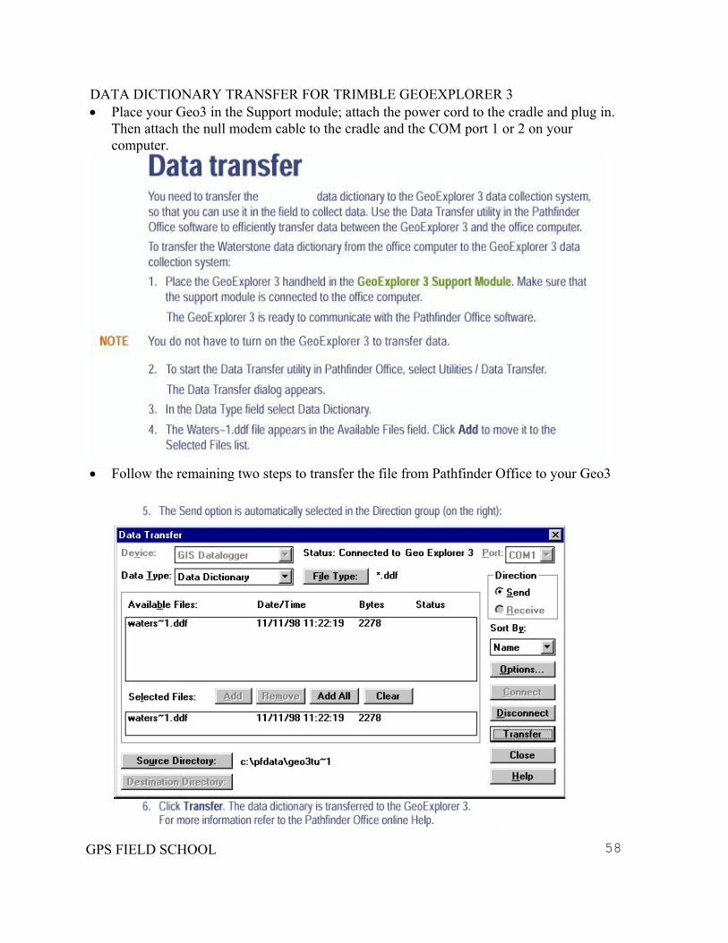
DATA DICTIONARY TRANSFER FOR TRIMBLE GEOEXPLORER 3 • Place your Geo3 in the Support module; attach the power cord to the cradle and plug in.

Then attach the null modem cable to the cradle and the COM port 1 or 2 on your computer.

• Follow the remaining two steps to transfer the file from Pathfinder Office to your Geo3

GPS FIELD SCHOOL 58

NOTES

GPS FIELD SCHOOL 59

Session 7: PROJECT FIELDWORK Most of you probably will use GPS to augment your daily tasks--to assist with resource identification and documentation, map areas of vegetation for monitoring and protection, add features to a baseline park inventory, map social trails that provide informal points of park access, or walk out the proposed course of a new hiking/interpretive trail. In many cases, you will be working alone, that is, fielding a single team. In some cases, though, it can be productive to bring in other teams from the region or neighboring parks to assist with a special mapping project. Because GPS equipment--and trained personnel--are usually in short supply, resource managers in neighboring parks should consider pooling resources and exchanging services. A multi-team GPS survey can be a complex logistical undertaking. A large project can be divided among teams by task or by sector. The project manager should

• write a project description • clearly delineate the tasks and expectations of each team • design and download a project data dictionary to each datalogger • discuss the importance of every item on the data dictionary • provide maps, documentation, and guides if needed • hold daily debriefing sessions, and • track daily progress on a master map.

There are many things that the crew leader can do to maximize efficiency and data quality. Field Time Rule Number 1 Always know where you are going. This is vital to the efficiency of the survey. Most people will only have a limited amount of time to spend in the field, and that time must be spent wisely. While the satellites are available, the GPS units should be moving. It is wasteful to spend field time searching for the next feature to map if this searching can be avoided. Do a reconnaissance before the survey begins, or assign at least two people to a team, one of whom can scout the next feature to map. Field Time Rule Number 2 Know your data dictionary. Time is wasted looking for the right feature in a data dictionary. If the surveyors know the data dictionary, know what features are called and where things are located, the mapping goes much faster. All field crews should review the data dictionary before setting out. Field Time Rule Number 3 Know what you are mapping. If the surveyors are unfamiliar with the resources, it is very important that a knowledgeable person accompany the crew if you are to get accurate data. This applies not only to recognizing the physical feature, but properly recording the attributes. At the very least, a printed copy of the data dictionary along with descriptions of each attribute and how to assess it should be part of every field kit.

GPS FIELD SCHOOL 60

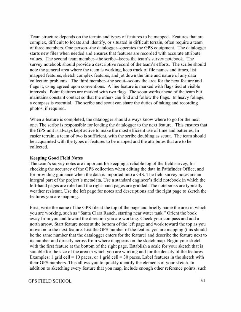
Team structure depends on the terrain and types of features to be mapped. Features that are complex, difficult to locate and identify, or situated in difficult terrain, often require a team of three members. One person--the datalogger--operates the GPS equipment. The datalogger starts new files when needed and ensures that features are recorded with accurate attribute values. The second team member--the scribe--keeps the team’s survey notebook. The survey notebook should provide a descriptive record of the team’s efforts. The scribe should note the general area where the team is working, keep track of file names and times, list mapped features, sketch complex features, and jot down the time and nature of any data collection problems. The third member--the scout--scours the area for the next feature and flags it, using agreed upon conventions. A line feature is marked with flags tied at visible intervals. Point features are marked with two flags. The scout works ahead of the team but maintains constant contact so that the others can find and follow the flags. In heavy foliage, a compass is essential. The scribe and scout can share the duties of taking and recording photos, if required. When a feature is completed, the datalogger should always know where to go for the next one. The scribe is responsible for leading the datalogger to the next feature. This ensures that the GPS unit is always kept active to make the most efficient use of time and batteries. In easier terrain, a team of two is sufficient, with the scribe doubling as scout. The team should be acquainted with the types of features to be mapped and the attributes that are to be collected. Keeping Good Field Notes The team’s survey notes are important for keeping a reliable log of the field survey, for checking the accuracy of the GPS collection when editing the data in Pathfinder Office, and for providing guidance when the data is imported into a GIS. The field survey notes are an integral part of the project’s metadata. Use a standard engineer’s field notebook in which the left-hand pages are ruled and the right-hand pages are gridded. The notebooks are typically weather resistant. Use the left page for notes and descriptions and the right page to sketch the features you are mapping. First, write the name of the GPS file at the top of the page and briefly name the area in which you are working, such as “Santa Clara Ranch, starting near water tank.” Orient the book away from you and toward the direction you are working. Check your compass and add a north arrow. Start feature notes at the bottom of the left page and work toward the top as you move on to the next feature. List the GPS number of the feature you are mapping (this should be the same number that the datalogger enters for the feature) and describe the feature next to its number and directly across from where it appears on the sketch map. Begin your sketch with the first feature at the bottom of the right page. Establish a scale for your sketch that is suitable for the size of the area in which you are working and for the density of the features. Examples: 1 grid cell = 10 paces, or 1 grid cell = 30 paces. Label features in the sketch with their GPS numbers. This allows you to quickly identify the elements of your sketch. In addition to sketching every feature that you map, include enough other reference points, such

GPS FIELD SCHOOL 61

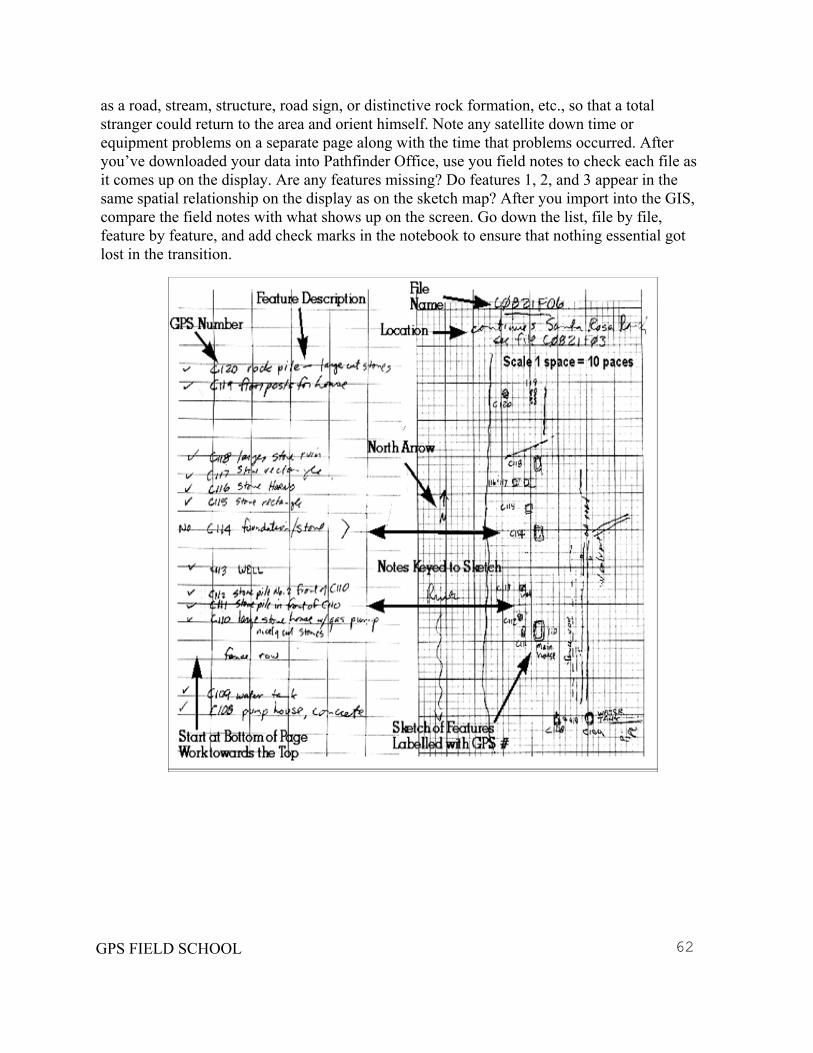
as a road, stream, structure, road sign, or distinctive rock formation, etc., so that a total stranger could return to the area and orient himself. Note any satellite down time or equipment problems on a separate page along with the time that problems occurred. After you’ve downloaded your data into Pathfinder Office, use you field notes to check each file as it comes up on the display. Are any features missing? Do features 1, 2, and 3 appear in the same spatial relationship on the display as on the sketch map? After you import into the GIS, compare the field notes with what shows up on the screen. Go down the list, file by file, feature by feature, and add check marks in the notebook to ensure that nothing essential got lost in the transition.

GPS FIELD SCHOOL 62

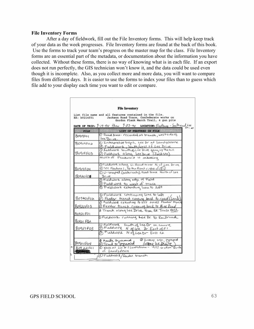
File Inventory Forms After a day of fieldwork, fill out the File Inventory forms. This will help keep track of your data as the week progresses. File Inventory forms are found at the back of this book. Use the forms to track your team’s progress on the master map for the class. File Inventory forms are an essential part of the metadata, or documentation about the information you have collected. Without these forms, there is no way of knowing what is in each file. If an export does not run perfectly, the GIS technician won’t know it, and the data could be used even though it is incomplete. Also, as you collect more and more data, you will want to compare files from different days. It is easier to use the forms to index your files than to guess which file add to your display each time you want to edit or compare.

GPS FIELD SCHOOL 63

Session 8: INTRODUCTION TO POST-PROCESSING Post-processing consists of:

1) downloading base files to your PC from either a bulletin board community base station (CBS) via modem or the Internet, or from a datalogger set up to operate as a base station; 2) downloading the rover files from the data logger to the computer; 3) selecting base and rover files for differential correction; 4) adjusting the reference position for the base station (if necessary); and 5) running differential correction.

SEVENTH EXERCISE: DIFFERENTIAL CORRECTION 1) Download Base Files Base station data may come in one big file that contains all of a day’s data or it may come packaged as hourly files. Hourly files downloaded from a CBS are tagged by “GPS time,” that is Greenwich Mean Time. You need to know how many hours west of GMT your current location is to determine which hourly files you need for correction. To convert GMT for this area: MST + 7:00 hours = GMT All CBS bulletin boards are not alike. Each has its own way of packaging and presenting the data for downloading. Most, however, provide step-by-step instructions on the codes and commands needed to accomplish the download. (If not, you will need to call the keeper of the base station and receive these instructions over the telephone.) A typical code might be: A8062111.ssf in which “A” is the base code, “8" the year, “06" the month, and “11" the hour covered by the file in GPS time. For this class we will use the base station at:

Colorado Plateau Field Station Flagstaff, Arizona http://www.usgs.nau.edu/gps/ Format: FYMMDDHH

For the following exercise, the instructors have acquired the base station data for you. Use Windows Explorer or DOS commands to copy the information from the diskette into the project subdirectory named “base” (for example: c:\pfdata\training\base). Pathfinder Office looks for base files in this subdirectory when it begins processing. 2) Download Rover Files Start Pathfinder Office and make sure you are in the right project. Download your rover files to the PC. Note: The most common mistake made in transferring data is to start transferring on the PC before getting the datalogger ready.

GPS FIELD SCHOOL 64

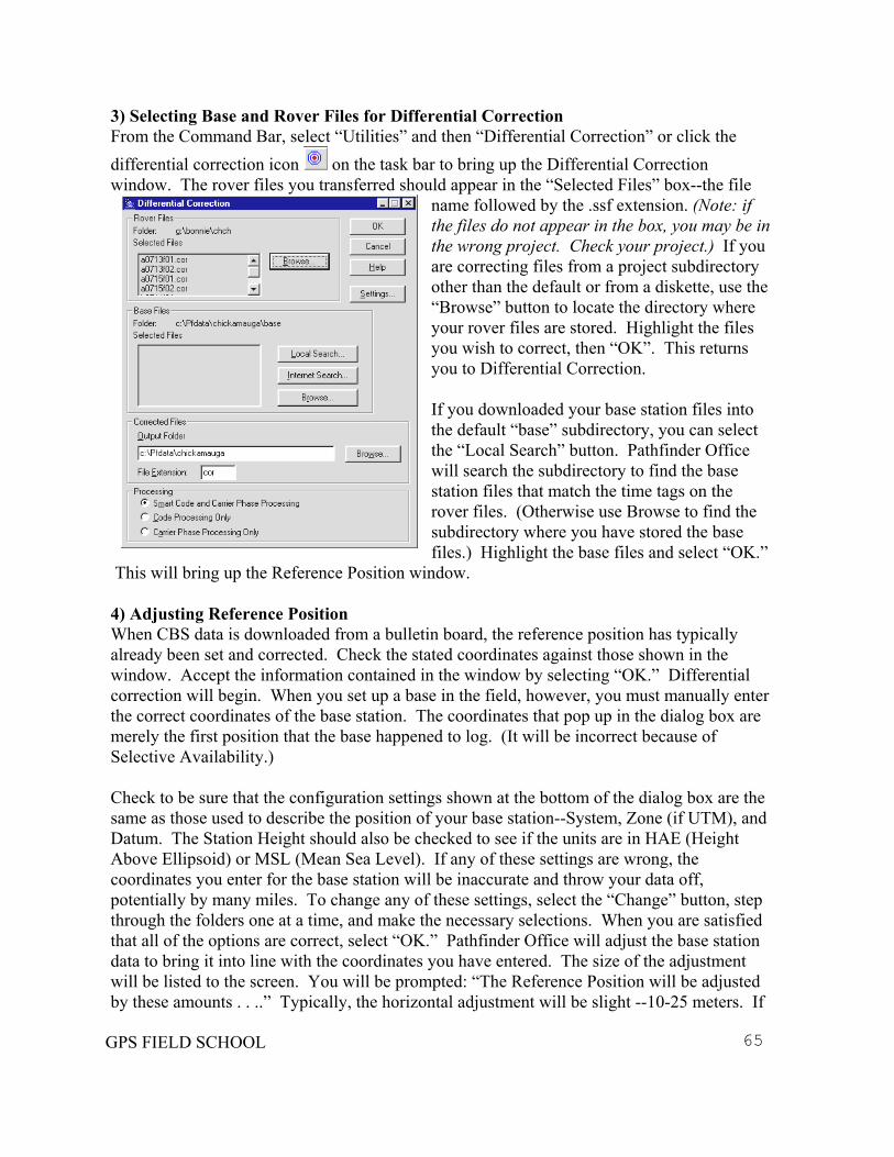
3) Selecting Base and Rover Files for Differential Correction From the Command Bar, select “Utilities” and then “Differential Correction” or click the differential correction icon on the task bar to bring up the Differential Correction window. The rover files you transferred should appear in the “Selected Files” box--the file

name followed by the .ssf extension. (Note: if the files do not appear in the box, you may be in the wrong project. Check your project.) If you are correcting files from a project subdirectory other than the default or from a diskette, use the “Browse” button to locate the directory where your rover files are stored. Highlight the files you wish to correct, then “OK”. This returns you to Differential Correction. If you downloaded your base station files into the default “base” subdirectory, you can select the “Local Search” button. Pathfinder Office will search the subdirectory to find the base station files that match the time tags on the rover files. (Otherwise use Browse to find the subdirectory where you have stored the base files.) Highlight the base files and select “OK.”

This will bring up the Reference Position window. 4) Adjusting Reference Position When CBS data is downloaded from a bulletin board, the reference position has typically already been set and corrected. Check the stated coordinates against those shown in the window. Accept the information contained in the window by selecting “OK.” Differential correction will begin. When you set up a base in the field, however, you must manually enter the correct coordinates of the base station. The coordinates that pop up in the dialog box are merely the first position that the base happened to log. (It will be incorrect because of Selective Availability.)

GPS FIELD SCHOOL 65

Check to be sure that the configuration settings shown at the bottom of the dialog box are the same as those used to describe the position of your base station--System, Zone (if UTM), and Datum. The Station Height should also be checked to see if the units are in HAE (Height Above Ellipsoid) or MSL (Mean Sea Level). If any of these settings are wrong, the coordinates you enter for the base station will be inaccurate and throw your data off, potentially by many miles. To change any of these settings, select the “Change” button, step through the folders one at a time, and make the necessary selections. When you are satisfied that all of the options are correct, select “OK.” Pathfinder Office will adjust the base station data to bring it into line with the coordinates you have entered. The size of the adjustment will be listed to the screen. You will be prompted: “The Reference Position will be adjusted by these amounts . . ..” Typically, the horizontal adjustment will be slight --10-25 meters. If

it is above 100 meters, though, you may have made a mistake entering the coordinates. Cancel. Go back and double check all your settings and values. When you are satisfied that everything is in order. Select “OK” and “OK” again to accept the base station adjustment. Differential correction will now begin.

Note: if you accidentally adjust a base station to the wrong coordinates you will need to delete the file and reload an unadjusted version. Trying to readjust the file will compound the error.

5) Running Differential Correction After the base and rover files are processed and compared, the results box will pop up showing the number of positions and features that were corrected. This dialog box will also tell you why positions did not correct. For example, the box will tell you that:

6 files processed. In these files: 96% of the uncorrected positions were corrected. 1878 positions were read. 1803 positions were corrected. 30 features were corrected. 3 features did not correct.

Select “More Details” for a description of which features did not correct and the reasons why. You might learn that:

There were 317 positions in file B0712f02. Of those, 298 were corrected. 7 positions were collected before the base station was operating. 3 positions were discarded because of faulty rover data. 6 discarded because a satellite used by the rover was missing in the base constellation. 4 positions were collected after the base station was shut down.

Files that contain positions that were collected before the base was turned on or after it was turned off can be run through the process again if you find base station files with the correct time tags. You must recorrect the entire file with correction data from a single base station. If your chosen base doesn’t have the data you need, you must go to another base and get all of the files to correct your rover file from that new base. Recorrect the entire rover file against this new base data. After you have studied the log files, “Close” out of differential correction and go to the main Pathfinder Office window. To view the files you have just corrected, select “Files” and “Open” from the Command Bar. This will bring up the files in your subdirectory.

GPS FIELD SCHOOL 66

Files are stored on the datalogger without an extension (e.g., a1023f01). When these files are transferred into Pathfinder Office, the program translates them into Trimble’s standard storage format and adds an .ssf file extension (e.g., a1023f01.ssf). The process of differential correction corrects for SA and changes the .ssf extension to a .cor (e.g., a1023f01.cor). You will now have two sets of files in your subdirectory -- an uncorrected set with the .ssf extension, and a corrected set with the .cor extension. You may view these files, by highlighting all of them and selecting “OK.” If you wish to edit positions, however, you can only work on one file at a time. Highlight and open the file you want to edit and bring the others in as background coverages. Because of the various sources of error in GPS collection, it is necessary to inspect and edit the “raw” data after differential correction. In Pathfinder Office, you cannot add positions, only take them away. Thus, the editing task is to identify problem features and delete positions that are obviously deviant. The next session will introduce you to file editing techniques.

GPS FIELD SCHOOL 67

Session 9: INTRODUCTION TO FILE EDITING Because of the various sources of error in GPS collection, it is necessary to inspect and edit the data after differential correction. In Pathfinder Office, you cannot add positions, only take them away. This prevents surveyors from altering or falsifying data (not that any would). Thus, the editing task is to identify problem features and delete positions that are obviously deviant. How do we tell good data from bad data? Ask whether the data was collected properly. Were there equipment problems? Were mistakes made in collection? Consult your field notes to see whether the satellites were cooperating (low PDOP, steady acquisitions). Do all of the collected features line up with your reference features on the display? Does the appearance of the display match your field sketches and memory? It is best to edit a day’s data before collecting new data. The sooner you look at features in Pathfinder Office, the clearer recall you will have of the sites and situations surrounding the data collection. The longer data sits unedited, the less accurate the editing, the more suspect the information. Point features require no editing, but do require scrutiny. Does this monument line up with the road and other monuments, for example? If it seems misplaced, consult your notes for this file. Were you having trouble receiving satellites? Was the PDOP very high, spiking in and out? Was there operator error? If you conclude that a point feature is misplaced, make a note on your file inventory sheet and go back out to the field to re-map the point. Or, add the file again, displaying positions rather than features. Examine the pattern. If one or more positions seem far out of line, delete these positions, save the file, and display the features again. Line and Area features sometimes require extensive editing. The straight sidewalk that you remember may show up on the display as a zigzag or appear to have thorns like a rose stem. Relying on the Beginning and End Points that you collected in the field, you can reliably straighten out the line by deleting the zigs or stripping the thorns. The result will be a straight line that follows the trend of the majority of positions captured in the feature. Nested angle points alert you to actual bends and angles in the line. If you stood in one place too long while collecting positions, a line might actually tie itself into knots. Unravel the knots by deleting the extra positions. (This can be avoided by using PAUSE button in the field.) In the Display Screen under Data, you will find Feature Properties and Position Properties. The Feature Properties window allows you to review and edit the data displayed. The Position Properties window lets you examine individual (GPS) positions in a data file. Use the Positions Properties when you want to remove positions. Use the Feature Properties to remove entire features. A pop-up window will appear asking for confirmation to delete the current feature, if you respond yes, the feature will disappear and the Delete key will turn into the Undelete key. A deleted feature is still present in the data file, and you can undelete it. Pathfinder Office does not display deleted features or notes and they do not appear in data output to a GIS.

GPS FIELD SCHOOL 68

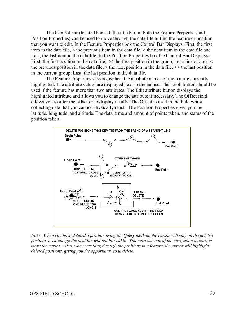
The Control bar (located beneath the title bar, in both the Feature Properties and Position Properties) can be used to move through the data file to find the feature or position that you want to edit. In the Feature Properties box the Control Bar Displays: First, the first item in the data file, < the previous item in the data file, > the next item in the data file and Last, the last item in the data file. In the Position Properties box the Control Bar Displays: First, the first position in the data file, << the first position in the group, i.e. a line or area, < the previous position in the data file, > the next position in the data file, >> the last position in the current group, Last, the last position in the data file. The Feature Properties screen displays the attribute names of the feature currently highlighted. The attribute values are displayed next to the names. The scroll button should be used if the feature has more than two attributes. The Edit attribute button displays the highlighted attribute and allows you to change the attribute if necessary. The Offset field allows you to alter the offset or to display it fully. The Offset is used in the field while collecting data that you cannot physically reach. The Position Properties gives you the latitude, longitude, and altitude. The data, time and amount of points taken, and status of the position taken.

Note: When you have deleted a position using the Query method, the cursor will stay on the deleted position, even though the position will not be visible. You must use one of the navigation buttons to move the cursor. Also, when scrolling through the positions in a feature, the cursor will highlight deleted positions, giving you the opportunity to undelete.

GPS FIELD SCHOOL 69

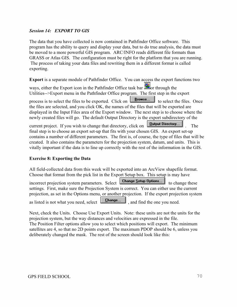
Session 14: EXPORT TO GIS The data that you have collected is now contained in Pathfinder Office software. This program has the ability to query and display your data, but to do true analysis, the data must be moved to a more powerful GIS program. ARC/INFO reads different file formats than GRASS or Atlas GIS. The configuration must be right for the platform that you are running. The process of taking your data files and rewriting them in a different format is called exporting. Export is a separate module of Pathfinder Office. You can access the export functions two

ways, either the Export icon in the Pathfinder Office task bar or through the Utilities-->Export menu in the Pathfinder Office program. The first step in the export

process is to select the files to be exported. Click on to select the files. Once the files are selected, and you click OK, the names of the files that will be exported are displayed in the Input Files area of the Export window. The next step is to choose where the newly created files will go. The default Output Directory is the export subdirectory of the

current project. If you wish to change that directory, click on . The final step is to choose an export set-up that fits with your chosen GIS. An export set-up contains a number of different parameters. The first is, of course, the type of files that will be created. It also contains the parameters for the projection system, datum, and units. This is vitally important if the data is to line up correctly with the rest of the information in the GIS. Exercise 8: Exporting the Data All field-collected data from this week will be exported into an ArcView shapefile format. Choose that format from the pick list in the Export Setup box. This setup is may have

incorrect projection system parameters. Select to change these settings. First, make sure the Projection System is correct. You can either use the current projection, as set in the Options menu, or another projection. If the export projection system

as listed is not what you need, select , and find the one you need. Next, check the Units. Choose Use Export Units. Note: these units are not the units for the projection system, but the way distances and velocities are expressed in the file. The Position Filter options allow you to select which positions will export. The minimum satellites are 4, so that no 2D points export. The maximum PDOP should be 6, unless you deliberately changed the mask. The rest of the screen should look like this:

GPS FIELD SCHOOL 70

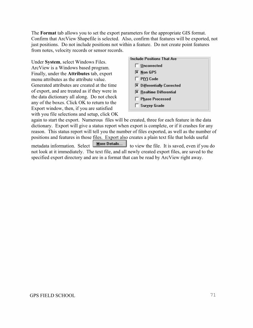
The Format tab allows you to set the export parameters for the appropriate GIS format. Confirm that ArcView Shapefile is selected. Also, confirm that features will be exported, not just positions. Do not include positions not within a feature. Do not create point features from notes, velocity records or sensor records. Under System, select Windows Files. ArcView is a Windows based program. Finally, under the Attributes tab, export menu attributes as the attribute value. Generated attributes are created at the time of export, and are treated as if they were in the data dictionary all along. Do not check any of the boxes. Click OK to return to the Export window, then, if you are satisfied with you file selections and setup, click OK again to start the export. Numerous files will be created, three for each feature in the data dictionary. Export will give a status report when export is complete, or if it crashes for any reason. This status report will tell you the number of files exported, as well as the number of positions and features in those files. Export also creates a plain text file that holds useful

metadata information. Select to view the file. It is saved, even if you do not look at it immediately. The text file, and all newly created export files, are saved to the specified export directory and are in a format that can be read by ArcView right away.

GPS FIELD SCHOOL 71

Some Basic GIS Concepts Although we have been working with spatial data throughout this course in Pathfinder Office®, your GPS data will ultimately reside in a GIS or geographic information system. Learning to collect your cultural/natural resource information, or any other features such as utilities, with GPS remains the goal of this fieldschool. However, using this data, once captured, will become your eventual priority. The GIS will be the tool you use to view your GPS data, manipulate the information, combine the GPS data with other digital information, or query your data in order to answer your daily questions. A GIS consists of a combination of elements including, hardware, software and data, in addition to the people and methods required to make the GIS work. Together, all of these elements create an interactive and powerful mapping application. GIS hardware encompasses the computer, as well as input devices (such as digitizers, scanners or GPS) and output devices (such as printers or plotters). To maintain and use this hardware, you will need to establish and follow a methodology for collecting data and utilizing your GIS, in addition to finding people with GIS skills. Most of all, you will need spatial data and GIS software to provide the tools to display, analyze and manipulate your data. Broken down into these component elements, it becomes clear where your GPS, the data you collect with the GPS, and GIS will fit into your overall resource management plan. All GIS works by abstracting the three-dimensional world into a series of two-dimensional map layers. We already encountered this concept when editing GPS data in Pathfinder Office®, where you looked at individual feature types as different data layers. Through a similar overlay technique in the GIS, each data type or theme, such as topography, waterways, road networks or cultural resources, is represented as a layer of data. Individual features, represented as points, lines or polygons, make up the data layers themselves. The power of GIS lies in its ability to link each individual feature within a data layer to the information describing that feature, or attribute data. We entered all our own attribute data into the datalogger while we collected our coordinates with GPS receiver. Other spatial data you may use in the GIS also contains similar attribute information. The functionality of the GIS will allow us to manipulate this information, edit it and add to it. Additionally, we can use this attribute information to ask and answer questions. GIS Software Many versions of GIS software exist, and all of them comprise similar tools, allowing users to manage, analyze and display digital spatial and attribute information. Most GIS packages contain a database management system for the attribute information, tools to query both spatially and tabularly, spatial analysis tools, display tools for the spatial data and a graphical user interface for users to interact with.

GPS FIELD SCHOOL 72

The Environmental Systems Research Institute (ESRI) is the largest producer of GIS

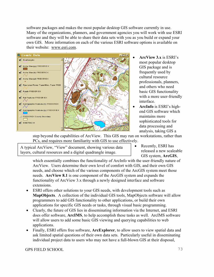
software packages and makes the most popular desktop GIS software currently in use. Many of the organizations, planners, and government agencies you will work with use ESRI software and they will be able to share their data sets with you as you build or expand your own GIS. More information on each of the various ESRI software options is available on their website: www.esri.com.

• ArcView 3.x is ESRI’s

most popular desktop GIS package and is frequently used by cultural resource professionals, planners, and others who need basic GIS functionality with a more user-friendly interface.

• ArcInfo is ESRI’s high-end GIS software which maintains more sophisticated tools for data processing and analysis, taking GIS a

step beyond the capabilities of ArcView. This GIS may run on workstations, rather than PCs, and requires more familiarity with GIS to use effectively.

A typical ArcView, “View” document, showing various data layers, cultural resources and a digital quadrangle image.

• Recently, ESRI has released a new scaleable GIS system, ArcGIS,

which essentially combines the functionality of ArcInfo with the user-friendly nature of ArcView. Users determine their own level of comfort with GIS, and their own GIS needs, and choose which of the various components of the ArcGIS system meet those needs. ArcView 8.1 is one component of the ArcGIS system and expands the functionality of ArcView 3.x through a newly designed interface and software extensions.

• ESRI offers other solutions to your GIS needs, with development tools such as MapObjects. A collection of the individual GIS tools, MapObjects software will allow programmers to add GIS functionality to other applications, or build their own applications for specific GIS needs or tasks, through visual basic programming.

• Clearly, the future of GIS lies in disseminating information via the Internet, and ESRI does offer software, ArcIMS, to help accomplish these tasks as well. ArcIMS software will allow users to add some basic GIS viewing and querying capabilities to web applications.

GPS FIELD SCHOOL 73

• Finally, ESRI offers free software, ArcExplorer, to allow users to view spatial data and ask limited spatial questions of their own data sets. Particularly useful in disseminating individual project data to users who may not have a full-blown GIS at their disposal,

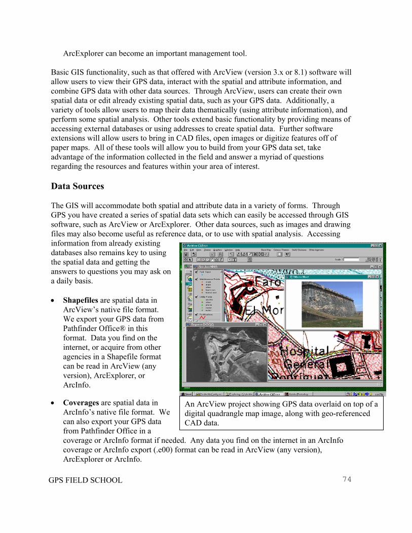
ArcExplorer can become an important management tool. Basic GIS functionality, such as that offered with ArcView (version 3.x or 8.1) software will allow users to view their GPS data, interact with the spatial and attribute information, and combine GPS data with other data sources. Through ArcView, users can create their own spatial data or edit already existing spatial data, such as your GPS data. Additionally, a variety of tools allow users to map their data thematically (using attribute information), and perform some spatial analysis. Other tools extend basic functionality by providing means of accessing external databases or using addresses to create spatial data. Further software extensions will allow users to bring in CAD files, open images or digitize features off of paper maps. All of these tools will allow you to build from your GPS data set, take advantage of the information collected in the field and answer a myriad of questions regarding the resources and features within your area of interest. Data Sources The GIS will accommodate both spatial and attribute data in a variety of forms. Through GPS you have created a series of spatial data sets which can easily be accessed through GIS software, such as ArcView or ArcExplorer. Other data sources, such as images and drawing files may also become useful as reference data, or to use with spatial analysis. Accessing information from already existing databases also remains key to using the spatial data and getting the answers to questions you may ask on a daily basis. • Shapefiles are spatial data in

ArcView’s native file format. We export your GPS data from Pathfinder Office® in this format. Data you find on the internet, or acquire from other agencies in a Shapefile format can be read in ArcView (any version), ArcExplorer, or ArcInfo.

An ArcView project showing GPS data overlaid on top of a digital quadrangle map image, along with geo-referenced CAD data.

• Coverages are spatial data in ArcInfo’s native file format. We can also export your GPS data from Pathfinder Office in a coverage or ArcInfo format if needed. Any data you find on the internet in an ArcInfo coverage or ArcInfo export (.e00) format can be read in ArcView (any version), ArcExplorer or ArcInfo.

GPS FIELD SCHOOL 74

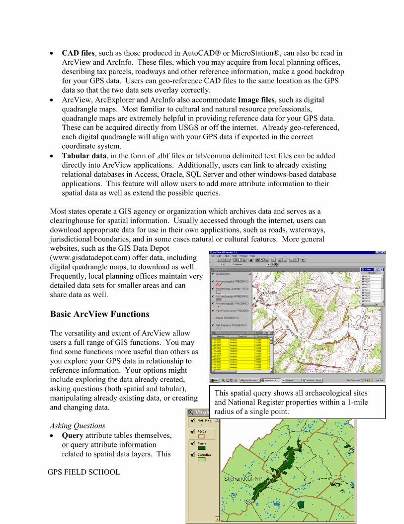
• CAD files, such as those produced in AutoCAD® or MicroStation®, can also be read in ArcView and ArcInfo. These files, which you may acquire from local planning offices, describing tax parcels, roadways and other reference information, make a good backdrop for your GPS data. Users can geo-reference CAD files to the same location as the GPS data so that the two data sets overlay correctly.

• ArcView, ArcExplorer and ArcInfo also accommodate Image files, such as digital quadrangle maps. Most familiar to cultural and natural resource professionals, quadrangle maps are extremely helpful in providing reference data for your GPS data. These can be acquired directly from USGS or off the internet. Already geo-referenced, each digital quadrangle will align with your GPS data if exported in the correct coordinate system.

• Tabular data, in the form of .dbf files or tab/comma delimited text files can be added directly into ArcView applications. Additionally, users can link to already existing relational databases in Access, Oracle, SQL Server and other windows-based database applications. This feature will allow users to add more attribute information to their spatial data as well as extend the possible queries.

Most states operate a GIS agency or organization which archives data and serves as a clearinghouse for spatial information. Usually accessed through the internet, users can download appropriate data for use in their own applications, such as roads, waterways, jurisdictional boundaries, and in some cases natural or cultural features. More general websites, such as the GIS Data Depot (www.gisdatadepot.com) offer data, including digital quadrangle maps, to download as well. Frequently, local planning offices maintain vdetailed data sets for smaller areas and can share data as well.

ery

Basic ArcView Functions

75

The versatility and extent of ArcView allow users a full range of GIS functions. You may find some functions more useful than others as you explore your GPS data in relationship to reference information. Your options might include exploring the data already created, asking questions (both spatial and tabular), manipulating already existing data, or creating and changing data.

This spatial query shows all archaeological sites and National Register properties within a 1-mile radius of a single point.

Asking Questions

GPS FIELD SCHOOL

• Query attribute tables themselves, or query attribute information related to spatial data layers. This

will result in selecting features on your screen which meet a certain criteria that you define, such as locating all the buildings built between 1800 and 1850, or locating all the archaeological sites related to a specific cultural affiliation.

• Theme on theme selection using the spatial data to ask questions. This function uses one theme to ask a question of a second, such as, “find all the national register properties within 100 meters of a roadway.” Theme on theme selections allow users to take advantage of the geography to ask questions, something that can only be done with a GIS.

Manipulating Data

Users can quickly and easily draw their own spatial data, using other reference information, such as tax parcels or digital quadrangle maps. This is particularly helpful when drawing project boundaries.

• Spatial joins use the relationship between two themes to answer questions. This function joins together the attribute

tinuous line, for example.

attribute information again to combine featuwould allow users to join all the line segmensingle con

• Buffering features allows users to generaliaround their features. This function would awith GPS representing archaeological sites, instance.

Creating Data • Creating new shapefiles and editing shapef

Users can draw directly on-screen, using refquadrangle maps. Similar to the data collecor polygons and attach their own attributes tusers may reshape, delete or alter any of theacquired from other sources may be edited aCAD files may not. Coverages and CAD fithen edited however.

GPS FIELD SCHOOL

• Geo-Coding functions allow users to create

Performing a spatial join with this data would allow users to find all the NationalRegister sites within park boundaries,

information of different data layers, using the geographySpatial joins are particulahelpful when determining inside or nearest relationship For example, users couuse a join to determine what congressional district each of their resources fell withdetermine the nearest national reg

. rly an

. ld

in, or

ister property to

•

ate a

their park. Merging features uses the

res within a single data layer. Merging ts forming “Main St.” together to cre

ze their data, or examine an area directly llow users to generalize points collected creating larger areas defined by a radius, for

iles is a simple process within the GIS. erence information, such as digital ted with GPS, users may create points, lines o each feature as it is created. Once drawn, spatial data on-screen as well. Shapefiles s well, although coverages, images and

les may be converted into shapefiles first,

76

point data from a table of addresses. Using

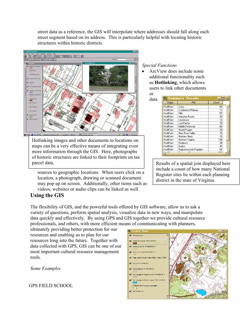
street data as a reference, the GIS will interpolate where addresses should fall along each street segment based on its address. This is particularly helpful with locating historic structures within historic districts.

Special Functions

Hotlinking images and other documents to locations on maps can be a very effective means of integrating even more information through the GIS. Here, photographs of historic structures are linked to their footprints on tax parcel data. Results of a spatial join displayed here

include a count of how many National Register sites lie within each planning district in the state of Virginia.

• ArcView does include some additional functionality such as Hotlinking, which allows users to link other documents or data

sources to geographic locations. When users click on a location, a photograph, drawing or scanned document may pop up on screen. Additionally, other items such as videos, websites or audio clips can be linked as well.

Using the GIS

77

The flexibility of GIS, and the powerful tools offered by GIS software, allow us to ask a variety of questions, perform spatial analysis, visualize data in new ways, and manipulate data quickly and effectively. By using GPS and GIS together we provide cultural resource professionals, and others, with more efficient means of communicating with planners, ultimately providing better protection for our resources and enabling us to plan for our resources long into the future. Together with data collected with GPS, GIS can be one of our most important cultural resource management tools. Some Examples

GPS FIELD SCHOOL

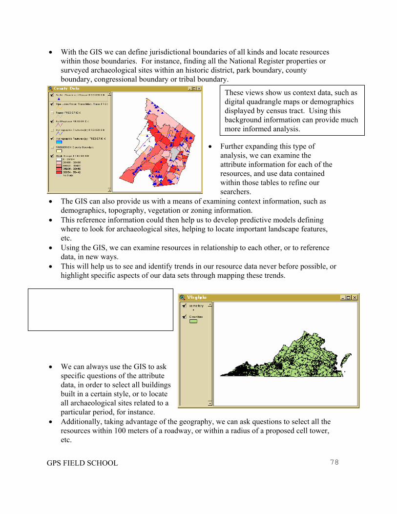
• With the GIS we can define jurisdictional boundaries of all kinds and locate resources within those boundaries. For instance, finding all the National Register properties or surveyed archaeological sites within an historic district, park boundary, county boundary, congressional boundary or tribal boundary.

•

• The GIS can also provide us with a means of examidemographics, topography, vegetation or zoning inf

• This reference information could then help us to dewhere to look for archaeological sites, helping to loetc.

• Using the GIS, we can examine resources in relatiodata, in new ways.

• This will help us to see and identify trends in our rehighlight specific aspects of our data sets through m

This view showing the distribution of cemeteries in Virginia indicates an interesting trend, which might lead to more research and further investigation.

GPS FIELD SCHOOL

• We can always use the GIS to ask

specific questions of the attribute data, in order to select all buildings built in a certain style, or to locate all archaeological sites related to a particular period, for instance.

• Additionally, taking advantage of the geography, wresources within 100 meters of a roadway, or withinetc.

These views show us context data, such asdigital quadrangle maps or demographics displayed by census tract. Using this background information can provide muchmore informed analysis.

Further expanding this type of analysis, we can examine the attribute information for each of the resources, and use data contained within those tables to refine our searchers. ning context information, such as ormation. velop predictive models defining cate important landscape features,

nship to each other, or to reference

source data never before possible, or apping these trends.

78

e can ask questions to select all the a radius of a proposed cell tower,

• We can further map out specific events, such as ARPA violations, to determine if there are specific areas targeted by thieves, or regions which require more attention and protection.

• Using the geography and the attributes together to ask questions in a variety of ways allows users to see their data in ways never before possible, and it allows us to develop a more efficient and means of communicating with planning professionals, resulting in better protection for our resources.

What Next Clearly, GIS and GPS together make powerful data collection and management tools for cultural resources, and any other resource type you may be interested in. These functions represent only a few of the possibilities available in ArcView, and other GIS software packages. You may want to investigate training in ArcView alone, or another GIS, to fully take advantage of the spatial data you collect using GPS. GIS will be one of the most important cultural resource management tools available to you in the future. Check the ESRI website (www.esri.com) for more information on their classes and course schedules/locations, or let CRGIS know of your interest in ArcView training. NOTES

GPS FIELD SCHOOL 79

NOTES

GPS FIELD SCHOOL 80

GPS FIELD SCHOOL 81