GOVERNMENT BORROWING AND MACROECONOMIC DYNAMICS OF

PAKISTAN

Authors: Dr. Mudassar Rashid, Muhammad Abeer Farooq, Dr. Shahzada M. Naeem Nawaz1

Sub-Theme: Macroeconomic Policies in a changing global and Local Landscape

ABSTRACT

Every economy employs certain procedures to address the growth and inflation dilemma. In the

capitalistic economies of present day, the objectives of sustained growth and minimal inflation

are achieved through the coordinated efforts of fiscal and monetary authorities. In developing

countries like Pakistan where both the authorities face the dilemma of meagre resources to

achieve their objectives, it is pertinent to study the effects of government borrowing on

macroeconomic dynamics. This study utilizes a modified New Keynesian Model to study the

impact of government borrowings on economic indicators like inflation, aggregate demand,

interest rate and exchange rate. In addition, the role of the State Bank of Pakistan in stabilization

of the economy by controlling government borrowing is also studied. Both Law of One Price and

Uncovered Interest Parity condition are relaxed. The data was taken for the period of 1975 to

2015. Rational expectation restrictions are identified by following Keating (1990). For

estimation purposes, Structural Vector Autoregressive (SVAR) model is used as to check the

structural changes with policy shocks. Johansen Cointegration (1990) is applied on the basis of

the results of unit root test of stationarity to check the long run association between the variables.

The responses of macroeconomic variables to government borrowing shocks and risk premium

shocks are assessed with impulse response function. Both the government borrowing and risk

premium shock have permanent positive effect on macroeconomic aggregates in the long run. An

effective monetary-fiscal coordination effort is needed to ensure the applicability of FDLA in its

true spirit.

Keywords: Monetary Policy, Fiscal Policy, Government Borrowing, SVAR, Impulse Response,

Risk Premium Shock

1 The authors are Assistant Professor, COMSATS, Islamabad; Research Fellow, Independent Researcher, Punjab

Economic Research Institute respectively.

1. INTRODUCTION

During the past thirty years, an important issue for the policy makers remains around the

repercussions of government borrowing on macroeconomic performance of a country. It is not

difficult to understand the reasons behind rapid rise in government borrowing in comparison to

GDP all over the world. History, prior to last three decades, witnesses rapid increase in the

government borrowing only during the depression periods or the war. However, the policy

makers, more or less, remains silent to devise policies to overcome this rising trend. This episode

raises a very relevant question, that is, what are the repercussions of government borrowing?

In Pakistan from the beginning of financial restructuring, the idea of monetary and fiscal policy

coordination is least bothered even in academic research. During 1973-90, domestic borrowings

was high because of fiscal policy failure. In 1990s, it is witnessed that there are many changes in

monetary authority rules and debt management rules. One of those changes is the change for

policy makers. That was conducting of monetary policy by central bank of Pakistan. It was a

modification in the State Bank of Pakistan Act, 1956, monetary policy conducting comes first

responsibility of SBP.

The economic policy should be organized in a way so as to provide stable economic growth

which is free from the impacts of inflation. So, to achieve those end results of economic policy,

there is need for coordination between fiscal and monetary authorities whose objectives are often

conflicting and contradictory. Keeping this in mind is always important as the autonomy of

central banks has been advocated in the past few decades due to the distrust in government's

policies to reduce inflation. As a result, the idea of 'independence of central banks' was

propagated to keep a check on inflation through monetary policy. The study aims to frame

theoretical model comprising impact of government borrowing on aggregate demand, exchange

rate, interest rate, inflation and other macroeconomic indicators so as to understand the role of

government borrowing in affecting macroeconomic dynamics of the economy of Pakistan.

Many times, governments take political decisions about the infrastructure development and the

projects which can be quoted for winning the upcoming elections. These politically motivated

decisions are normally rationalized economically. More specifically in the economy of Pakistan,

lack of independence of the monetary authority (which is State Bank of Pakistan) which, during

the last many years, is working under the fiscal dominance, the sustained fiscal deficit

historically and the popular decisions by the sitting governments are the major factors which

provide good base to analyze the economy. This study makes choice to adopt a New Keynesian

Model developed by Cebi (2012) for Turkey and recently verified numerically by Shahid et al

(2016). Based on this model, the study aims to make the policy analysis where in magnitude of

the relationship among the macroeconomic variables will also be focused on along with relying

on simulation analysis.

Much of the literature both for the developed and developing countries emphasis only partially

on impact of government borrowing on few of the macroeconomic indicators like economic

growth, inflation etc. The great evolution in macroeconomic modeling, after the happening of the

Oil price shock of 1973 that results in capturing the Lucas critique, has not been covered under

the topic. There is need to understand the short run dynamics of government borrowing through

New Keynesian model considering most theoretically sound models wherein these models

address the Lucas Critique efficiently. The literature on Pakistan is greatly missing in this

perspective. The current study will use the New Keynesian model wherein uncovered interest

parity condition and the assumption of law of one price will be relaxed. Both the Fiscal and

monetary policies framework will be included in the model so as to complete the model in all

dimensions. Thus, government purchases will be explicitly included in the aggregate demand

equation. Equation for fiscal solvency will also be a part of the model. The model developed by

Cebi (2012), who worked for Turkey, is adopted mostly.

In Section 2, theoretical framework along with model is discussed that depict most of the

channels through which government borrowing impact the economy. Section 3, discusses the

methodology and identification of rational expectation restrictions. Section 4 incorporates

analysis of estimated results and last section concludes the study and present policy

recommendations.

2. THEORETICAL FRAMEWORK

It is a matter of routine in macroeconomics to approximate the solutions to non-linear, DSGE

using linear techniques, ever since the works of Kydland and Prescott (1982) and King et al.

(1988). Certain aspects of the dynamic properties of complicated models are characterized by

linear approximation methods. The first-order approximations do give reasonable answers to

questions such as the identification and determination of equilibrium and magnitudes of second

moments of the endogenous variables, where the support of shocks riding aggregate fluctuations

is small and an internal stationary than solution exists.

Economists of the last two decades of the 20th

century began constructing the macroeconomic

models on the basis of microeconomic foundations of rational choice in response to Lucas

Critique. These models are known widely as dynamic stochastic general equilibrium

(DSGE) models. These models start by categorizing agents actively working in the economy, i.e.

firms, households and governments in a single or multiple countries, as well as technology,

preferences and budgetary constraints of each one of them. It is assumed that every economic

agent makes an optimal choice, after taking into consideration the prices and strategies of other

agents, for both the present and the future. By considering the decisions of the different kinds of

agents, all at a time; it is very much possible to ascertain the price which equates supply to

demand in every market. Hence, a kind of equilibrium self-consistency is embodied in these

models: given the prices that must be in parallel with the agent’s supply and demand, agents

choose optimally. With the use of these models, we can choice structural shocks from the

models.

2.1 Aggregate Demand Curve

According to Ricardian equivalence, any tax cut or increase in government spending, which may

result in increase in budget deficit, requires implementation of taxes in the future. Thus, the

rational consumers increase their savings to pay future taxes which neutralizes the impact of

decrease in government savings. Ultimately, there will be no impact on the national savings and

the other macroeconomic variables as well. However, the empirical failure of Ricardian

Equivalence is mainly due to presence of market imperfections specifically in the capital market.

Market imperfections ensure the rigidity of prices in the short run which results in increase in

aggregate demand as a result of any decrease in nominal interest rate and the subsequent real

interest rate. Thus, real interest rate has negative affect on the aggregate demand. Another

important implication of the change in interest rate is to affect the consumption smoothing

pattern of households. Depending on the direction of change in interest rate, inter-temporal

substitution in consumption play important role.

New Keynesian models have strong microeconomic foundations and derived through the

behavior of individual households and firms. Households have two primary roles to play, one is

the consumption and the other is the supply of labor services. Accordingly, the objective of

household is maximization of lifetime utility, that is, any decrease (increase) in consumption

(saving) in the current period ensures increase (decrease) in consumption (saving) in the next

period. Therefore, forward looking output gap is a natural ingredient of the demand equation.

Looking at the consumption basket of the consumer in an open economy framework ensures the

inclusion of imported goods in consumption. There is potential of influence of exchange rate

changes on the demand if law of one price does not hold. Therefore, change in exchange rate is

an important determinant of aggregate demand. However, the direction of influence is uncertain,

that is, exchange rate can have either positive or negative influence on demand. It depends on the

behavior of suppliers of imported goods whether they fully pass on the impact of exchange rate

changes to the consumers or not.

Changes in fiscal policy stance through changes in government spending significantly affect the

aggregate demand in the economy and leads to consumption led growth. Finally, the IS equation

includes the aggregate demand shock originated through the structure of the economy and from

the behavior of consumer. The IS equation closely resembles Clarida, Gali and Gertler (2001),

Gali and Monachelli (2005) and Cebi (2012).

[ ] … (2.1)

Equation 2.1 is in log-linearized form. Output gap is obtained after subtracting potential output

from the actual output which is actually the cyclic component of the output and represents

deviation from the natural level of output. It is obtained through employing Hodrick Prescot

filter, a built-in feature in Eviews 9. Deviation of the economy from the natural path depicts the

presence of some sort of rigidities in the market thus calls for role of fiscal and monetary policies

to stabilize the economy around the natural path, that is, the steady state. Real interest rate is

what the Wicksell call it natural real rate of interest.

2.2 Aggregate Supply Function/Phillips Curve Equation

The nature of inflation dynamics, which is the most distinctive feature of the new Keynesian

paradigm, is captured by the New Keynesian Phillips Curve, which is based on Calvo’s (1983)

model. According to this model, inflation is determined by expected future inflation and firm’s

real marginal costs. Two main issues highlighted include one, what measures needed to

administer real activity. Two, expectations are a central part that can affect the results. Cost-push

shock can be added with the marginal cost, which represents the imperfections in the labor

market [Nawaz and Ahmed (2015)].2 The increased government borrowing may also be financed

through seigniorage which results in high inflation. According to Sargent and Wallace (1981),

inflation is ultimately a fiscal phenomenon and not the monetary phenomenon. At the time of

servicing the borrowing, higher dead weight losses will be witnessed in comparison to the losses

witnessed at the time of accumulating the government borrowings. Political angle of the

government borrowing is also very important as it reduces the fiscal flexibility of the government

and the political dependence due to heavy reliance on international agencies like IMF (Wicksell,

1896; Feldstein, 1995 among others). Government borrowings may also shake the confidence of

foreign investors. Government borrowing has large effect on life cycle consumers in the long run

in the sense of crowding-out (Auerbach and Kotlikoff, 1987).

… (2.2)

Above equation is for inflation that depends upon expected inflation, output gap, and cost push

shocks. And further cost put shocks can be

, it is short run trade off between

inflation and output. This equation also infers that inflation is forward looking, that is, current

inflation is dependent on forward looking expectations of inflation. It means that when producer

sets the price future inflation is considered by him.

2.3 Uncovered Interest Parity

Assuming that the time-varying risk premium is negatively correlated with an expected

depreciation may explain the empirical facts; see Froot and Thaler (1990). McCallum (1994)

explains the apparent empirical failure of uncovered interest rate parity with the hypothesis that

2 Nawaz and Ahmed (2015). New Keynesian macroeconomic model and monetary policy in Pakistan. Pakistan

Development Review, 54(1), 55.

central banks systematically manage interest rate differentials to avoid frequent changes in the

exchange rate. So, it seems to be preferable to use more common approach to describe the

relationship between interest rate and exchange rate. Following Ball (1999), it is proposed that

we ease the uncovered interest parity condition and apply simple approach that just show the

proportionate relation between real interest rate and exchange rate and a random shock which

captures every exogenous variable that can affect the real exchange rate like foreign interest rate,

confidence on the part of investors, and expectations etc.

A rise in real interest rate will leads to appreciation in real exchange rate, thus make domestic

assets more attractive for the foreign as well as domestic investors. is autoregressive term.

2.4 Taylor Rule

The primary role of the central bank is to ensure the stability of the economy through

appropriately responding to inflation and output gap. The objective is primarily to minimize the

welfare losses. Government borrowing many times in developing countries like Pakistan may

result in significant welfare losses due to inflationary consequences for the economy that leads to

lowering the purchasing power of the consumer. Therefore, an additional role of the central bank

can be to prevent the economy from excessive government borrowing through increasing the

interest rate. It discourages the government borrowing due to high cost of borrowing. According

to fiscal Responsibility and Debt Limitation Act (2005) validated in 2012 by the parliament put

State Bank of Pakistan responsible to control the government debt. Thus, presumably SBP

respond to debt also along with responding to inflation and output gap. Kumhof et al (2008)

include both inflation and debt in the interest rate rule. Accordingly, the interest rate rule will

take the form as

represents the monetary shock and is assumed as AR process. Any monetary surprises by the

monetary authority can influence the macroeconomic indicators in an important direction to

achieve the desired objectives.

2.5 Fiscal Policy Rule

Output and debt stabilization are two primary objectives of fiscal authority. Following basic form

of fiscal rules (government spending and tax rules) adopted by Cebi (2012), we transform the lag

of government spending and taxes into forward looking components, depicting the forward-

looking behavior on the part of fiscal authority to smooth the economy. Therefore, fiscal

smoothing is assumed to be a part of objective of the fiscal authority. The forward-looking form

of fiscal policy reaction function in log linear form is as under:

( )[ ]

[ ]

Parameters ρg and ρτ denote the degree of fiscal smoothing. The greater the degree of fiscal

smoothing, the less will be the response of government spending and taxes to output gap and

debt. Parameters gy and τy demonstrate the sensitivities of government spending and tax to past

value of output gap. Parameters gb and τb correspond to feedback coefficients on unobservable

debt stock and

and are i.i.d. government spending and tax shocks, which represent the non-

systematic component of discretionary fiscal policy or discretionary exogenous deviations from

the fiscal rules.

The government issues nominal debt period-by-period in order to pay the principle and interest

on its existing debt and to fund any discrepancy between its spending and its tax revenues. The

model is completed by fiscal constraint. As in Cebi (2012), log linear solvency constraint can be

written as:

[

]

However, the fiscal constraint also includes the structural shock depicting any surprise increase

in fiscal deficit can influence the debt and through debt to other macroeconomic indicators. It

resembles a situation where fiscal authority enjoy debt over and above the maximum limit of

debt as is the case of Pakistan in the presence of fiscal dominance. In this state of affairs, the role

of monetary authority is critically important. Any lack in fiscal-monetary coordination leads to

welfare losses. Where, is nominal debt stock, and denote the debt

to GDP ratio and consumption to GDP ratio at steady state respectively.

3. METHODOLOGY AND IDENTIFICATION OF RESTRICTIONS

In the previous section, we have discussed the theoretical foundations of the impact of

government borrowing on the macroeconomic dynamics along with representation of the

theoretical equations which adopted to estimate.

Critique by Lucas in 1976, during the period when Orthodox Keynesian models proved fail,

proved as a revolutionary step in the area of macroeconomic modelling on one hand and the

unacceptable econometric models on the other hand. It was actually the rebirth of

Macroeconomics. As a result, more strong models having microeconomic foundations started

evolving and the innovation of econometric models soon after the inception of VAR models have

been witnessed. Since then VAR models have been the prime models for making policy analysis.

The transformation of VAR models into structural VAR models further strengthen the body of

literature on econometric modelling. Structural VAR models incorporate the economic theory

through a compatible mode. The basic point of caution to use structural VAR models for policy

analysis is equal number of equations and structural shocks, according to Gali (1999). The

procedure developed by Keating (1990) is used to identify the Rational Expectation restrictions.

This procedure has the feature to not put restrictions on the lag dynamics of the model. Recently,

this procedure is used by Nawaz and Ahmed (2015) and Leu (2011) to estimate the parameters.

3.1 Identification of Restrictions

DSGE model conforming NK framework in closed economic environment derived in the

previous section is reproduced below.

[ ] … 3.1

… 3.2

… 3.3

… 3.4

( )[ ]

… 3.5

[ ] … 3.6

[

]

… 3.7

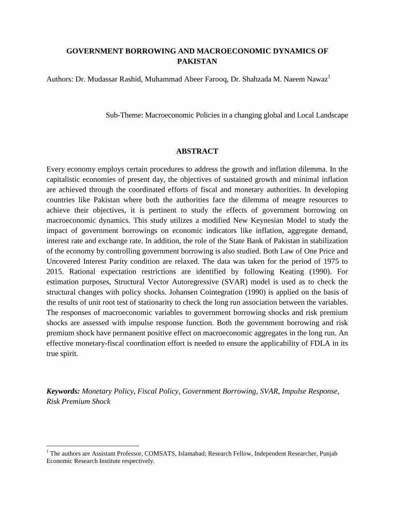
Subtracting all the variables in the above equations from their expected value at time ( )

yields the following set of equations:

“In the above equations, for all the variables represent the respective residual which

are residuals of reduced form VAR residuals. However, are the forward-

looking components in the model.

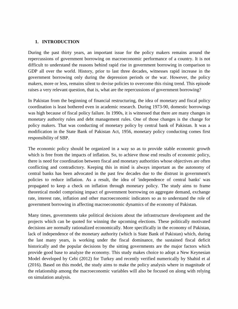
The procedure to calculate these forward looking components is elaborated as follows:”

[

]

[

]

[

]

[

]

(3.8)

(3.9)

“One step conditional expectation of equation (4.8) can be written in form as follows.”

(3.10)

“It may be considered that the expected value of residuals is equal to zero, i.e. .

As Y vector consists of all the endogenous variables, therefore to locate the variable of interest

(output gap and inflation), there is need to introduce vectors of length nq where n denotes the

number of endogenous variables and q denotes their lag order.”

for the output gap

for inflation

for Exchange Rate

for government expenditures

for taxes

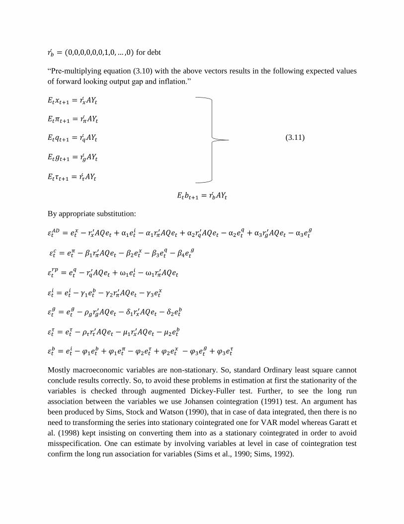
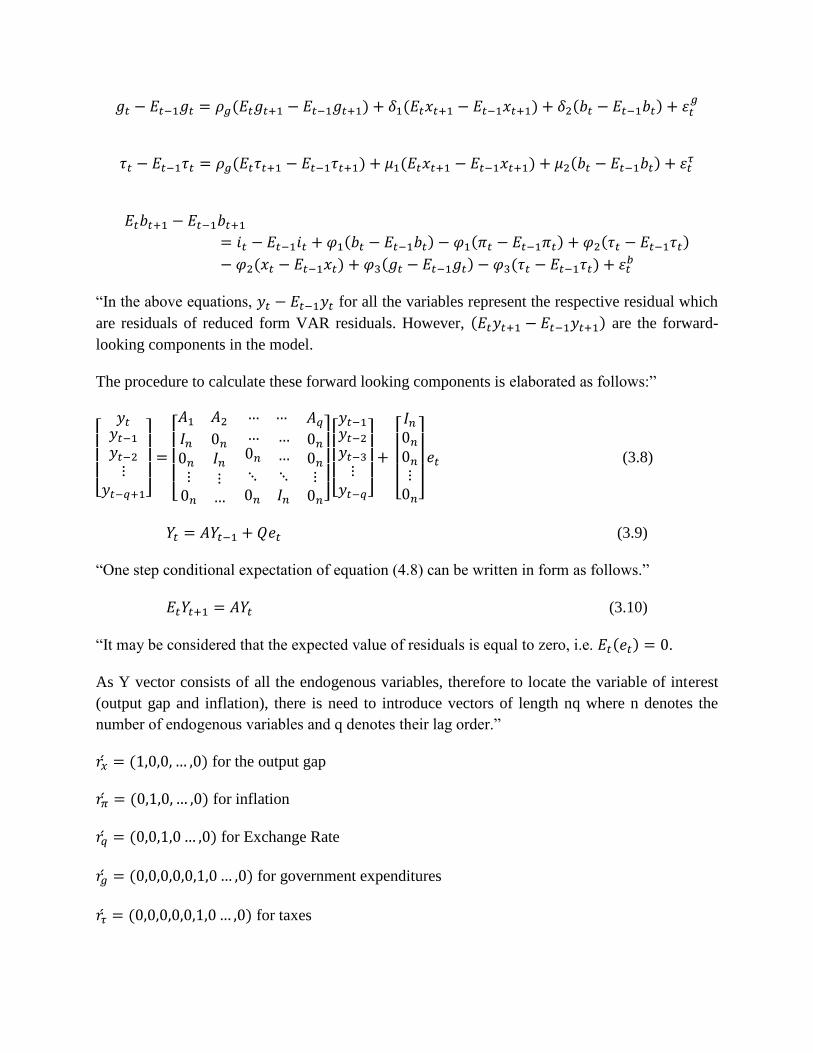
for debt

“Pre-multiplying equation (3.10) with the above vectors results in the following expected values

of forward looking output gap and inflation.”

(3.11)

By appropriate substitution:

Mostly macroeconomic variables are non-stationary. So, standard Ordinary least square cannot

conclude results correctly. So, to avoid these problems in estimation at first the stationarity of the

variables is checked through augmented Dickey-Fuller test. Further, to see the long run

association between the variables we use Johansen cointegration (1991) test. An argument has

been produced by Sims, Stock and Watson (1990), that in case of data integrated, then there is no

need to transforming the series into stationary cointegrated one for VAR model whereas Garatt et

al. (1998) kept insisting on converting them into as a stationary cointegrated in order to avoid

misspecification. One can estimate by involving variables at level in case of cointegration test

confirm the long run association for variables (Sims et al., 1990; Sims, 1992).

4. ESTIMATION RESULTS AND ANALYSIS

In this section, we estimate the New Keynesian model which is derived in above section. The

method for estimation procedure is SVAR which is appropriate to achieve our objectives.

Estimation is performed in Eviews 9 enterprises edition. Firstly, to check the stationarity of

variables we used unit root test, after that based on the results of unit root test we estimated the

long run association between the dependent and independent variables. The stationarity of the

variables is checked and found all the variables stationary at first order of integration. The results

are reported below in the table 4.1.

For analyzing long run relationship empirically among the macroeconomic variables used in our

model we adopted Johansen and Juselius’ (1990) system of cointegration test. The Trace test

statistics showed that there are seven coingtegration equations at 0.05 level are rejected the null

hypothesis of no long run association among variables. Whereas, Max-eigenvalue test indicates

five cointegration equations at the 0.05 level and rejecting the null hypothesis of no long run

association among variables. The results are reported in Appendix as table A-4.1 and A-4.2.

Table 4.1: Results of Unit Root Test

Variable At t-statistic Prob Order of integration

Output gap Level -1.53 0.512

1st difference -9.49*** 0.000 I(1)

R Level -2.01 0.06

1st difference -5.63*** 0.000 I(1)

Q (Risk

premium)

Level -2.36 0.120

1st difference -4.90*** 0.000 I(1)

Inf Level -2.41 0.144

1st difference -10.2*** 0.000 I(1)

Revenue gap Level -3.10 0.112

1st difference -4.57*** 0.000 I(1)

Expenditure

gap

Level -0.11 0.410

1st difference -5.33*** 0.000 I(1)

Debt gap Level -2.33 0.04

1st difference -4.31*** 0.00 I(1)

Note: ‘*’, ‘**’, ‘***’ shows the significance level at 10%, 5% and 1% respectively.

Critical values at 1%, 5% and 10% level of significance are: -4.521,-3.521 and -3.213

Various lag length criteria are used to obtain the optimal level of lag length for the VAR model.

The results show that the efficient lag length range is one as per AIC and all the diagnostic tests

are clear such as there is no evidence of serial correlation, heteroscedasticity and normality in

VAR (1, 1) model and given at appendix.

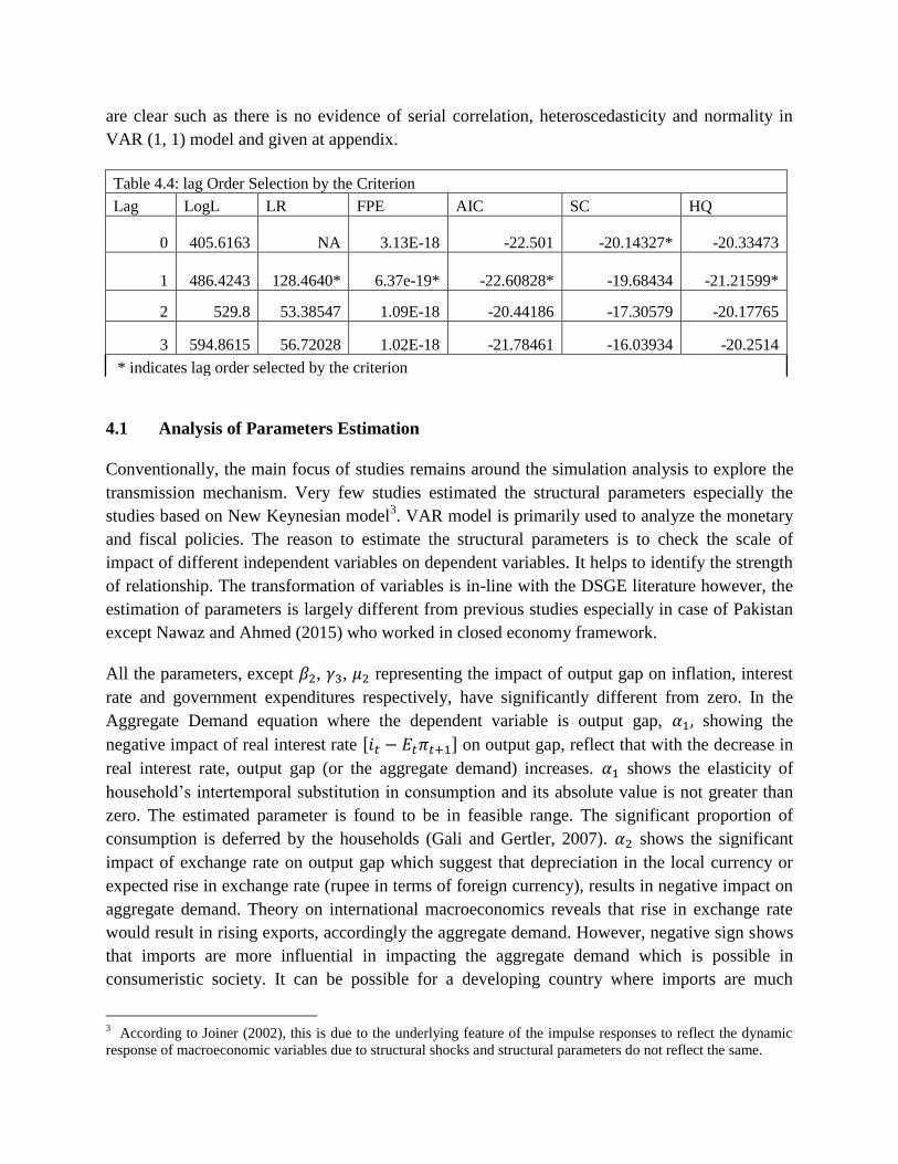
Table 4.4: lag Order Selection by the Criterion

Lag LogL LR FPE AIC SC HQ

0 405.6163 NA 3.13E-18 -22.501 -20.14327* -20.33473

1 486.4243

128.4640* 6.37e-19* -22.60828* -19.68434 -21.21599*

2 529.8 53.38547 1.09E-18 -20.44186 -17.30579 -20.17765

3 594.8615 56.72028 1.02E-18 -21.78461 -16.03934 -20.2514

* indicates lag order selected by the criterion

4.1 Analysis of Parameters Estimation

Conventionally, the main focus of studies remains around the simulation analysis to explore the

transmission mechanism. Very few studies estimated the structural parameters especially the

studies based on New Keynesian model3. VAR model is primarily used to analyze the monetary

and fiscal policies. The reason to estimate the structural parameters is to check the scale of

impact of different independent variables on dependent variables. It helps to identify the strength

of relationship. The transformation of variables is in-line with the DSGE literature however, the

estimation of parameters is largely different from previous studies especially in case of Pakistan

except Nawaz and Ahmed (2015) who worked in closed economy framework.

All the parameters, except , , representing the impact of output gap on inflation, interest

rate and government expenditures respectively, have significantly different from zero. In the

Aggregate Demand equation where the dependent variable is output gap, showing the

negative impact of real interest rate [ ] on output gap, reflect that with the decrease in

real interest rate, output gap (or the aggregate demand) increases. shows the elasticity of

household’s intertemporal substitution in consumption and its absolute value is not greater than

zero. The estimated parameter is found to be in feasible range. The significant proportion of

consumption is deferred by the households (Gali and Gertler, 2007). shows the significant

impact of exchange rate on output gap which suggest that depreciation in the local currency or

expected rise in exchange rate (rupee in terms of foreign currency), results in negative impact on

aggregate demand. Theory on international macroeconomics reveals that rise in exchange rate

would result in rising exports, accordingly the aggregate demand. However, negative sign shows

that imports are more influential in impacting the aggregate demand which is possible in

consumeristic society. It can be possible for a developing country where imports are much

3 According to Joiner (2002), this is due to the underlying feature of the impulse responses to reflect the dynamic

response of macroeconomic variables due to structural shocks and structural parameters do not reflect the same.

needed for the economy and exports are much vulnerable to the factors other than price.

indicates that with the expected rise in government expenditures in the next period, aggregate

demand in the current period decreases.

Table 4.5: Parameters Value with SVAR

Coefficient Std. Error z-Statistic Prob.

Aggregate Demand Equation

-0.0117 0.0006 -20.8941 0.0000

-2.2257 0.0257 -86.7065 0.0000

-0.3489 0.0068 -51.5630 0.0000

Phillips Curve Equation

0.5993 1.2683 0.4725 0.6366

3.2477 0.8890 3.6534 0.0003

0.6659 0.3148 2.1153 0.0344

UIP Equation

0.0285 0.0004 81.1189 0.0000

Taylor Rule

-0.1518 0.0311 -4.8878 0.0000

0.0023 0.0011 2.0030 0.0452

0.0646 0.0631 1.0243 0.3057

Fiscal Policy Rule

Government Expenditure Equation

2.8740 0.0275 104.5036 0.0000

5.1037 0.0778 65.5748 0.0000

-1.3633 0.0260 -52.4896 0.0000

Revenue Equation

1.9270 0.1059 18.1975 0.0000

-6.1009 0.5874 -10.3866 0.0000

0.1239 0.1354 0.9148 0.3603

Solvency Constraint

0.0295 0.0065 4.5228 0.0000

-0.2211 0.0200 -11.0309 0.0000

-0.0362 0.0118 -3.0775 0.0021

The impact of output gap on inflation is insignificant whereas the role of forward-looking

expectations is positively significant showing the forward-looking behavior on the part of firms

in deciding current period’s prices. It also depicts that inflation is primarily a cost-push

phenomenon in the country. The reason is obvious, that is, increasing cost of raw material,

energy and the imported goods used in the production process are the major reasons. The impact

of exchange rate on inflation is positively significant. It further strengthens the cost push nature

of inflation in the country as exchange rate being the component of marginal cost theoretically.

Government expenditures positively influence the inflation which shows that fiscal policy’s

impact on economic growth has cost of inflation for the economy. shows significant positive

impact of interest rate on exchange rate. Taylor (1993) provided a framework for rule based

monetary policy wherein he developed a response function depicting the response of interest rate

to inflation and demand changes. The parameters of interest rate rule show that State Bank of

Pakistan has not followed the Taylor rule during the period of investigation. This is something

critical and alarming in nature which due to inconsistency, involvement of time lag in response

or political factors results in failing to stabilize the economy or achieving the targeted levels of

macroeconomic indicators. Negative sign of debt parameter the reverse response of SBP, that is,

instead of increasing the interest rate to discourage the borrowing by the government, SBP

decreases the interest rate which confirms the fiscal dominance and the failure of implementation

of FDLA. However, as a matter of fact, SBP never claimed to follow the rule based policy as

also contended by Malik and Ahmed (2010).

With the increase in debt by the government, government expenditures decrease which is evident

from negative sign of . If the government expect that aggregate demand is increase in the next

period, it increases the expenditures in the current period which is reflection of growth strategy

of the government. It is depicted by the positive sign of . On the other hand, tax revenue

increases in response to increase in debt by the government which is evident from positive sign

of . With the increase in real debt in the current period, debt in the next period also increase.

Increase in tax- aggregate demand difference results in decreased debt in the next period.

Increase in fiscal deficit causes debt to decrease in future.

4.2 Impulse Response Analysis

In order to see the impulse responses in our model of different variables to output gap, it is given

the cholesky one S.D. innovations +/-2 S.E shock to dependent variables. At first, by giving the

shock to innovation in the aggregate demand equation output gap is dependent variable and

government borrowing shock affect the output gap. It depicts that the response of output gap is

increasing positively till one and a half year, then it tends to decline and after eight periods its

positive impact vanishes, showing no change in the output gap. The output gap is showing

positive behavior towards government borrowing shock. The impact of output gap to

government borrowing shock is as similar to the literature that government in order to meet the

budget deficit tends to take borrowing and it would lead to the aggregate demand that ultimately

results of increase the output gap of the country Schclarek.(2004).

4.2.1 Response of Macroeconomic indicators to Government Borrowing Shock

The government borrowing is availed in respect of access of government expenditure. Due to the

increase in the government borrowing the aggregate demand increase through investment and

consumption channel in the economy.

-.01

.00

.01

.02

2 4 6 8 10

Figure 1: Response of output gap to borrowing shock

As due to the increase in the government borrowing, the supply of money is increase in the

economy; if borrowing is done through printing of money, and it would ultimately lead to

increase in the inflationary pressure in the economy. Now, in context of Pakistan, the

government borrowing shows a positive relationship for first few years and then it soon reaches

to the steady state level and shows no impact over inflation in the economy.

-1

0

1

2 4 6 8 10

Figure 2: Response of inflation to Borrowing shock

In Figure 2, inflation is also showing increasing trend due to the government borrowing shock at

first year and after that it tends to decrease and reaches to the steady state level at fourth year.

The response of inflation to government borrowing shock is similar to the theory. Due to the

government borrowing the supply of money would increase in the economy. If borrowing is

through printing of money and this increase in money supply is create the inflationary pressure in

the economy (Yasmin et. al, 2013). It shows the positive behavior of inflation to the government

borrowing shock in the long run.

The impulse response of risk premium to government borrowing shock is negatively related at

first two periods. The risk premium goes down to the steady state level for first two periods. At

third periods, its moves upward from the steady state level and for further four periods it has a

positive impact. It shows that the any shock to government budget borrowing is responsible

negative association to the risk premium and it also validated by the literature that with the

increase in the government budget borrowing there happens two-fold impacts, at first the

exchange rate declines and the second one is inflation advances forward.

-.01

.00

.01

.02

.03

2 4 6 8 10

Figure 3: Response of Risk Premium to Borrowing Shock

As due to increase in the government borrowing the interest rate is crease making crowding out

effect. This has negative impact over output gap as due to increase in the interest rate the

aggregate demand would shrink. And similar effect can be analyzed for first two periods in case

of Pakistan through impulse response function given in the Figure 4 below:

-.08

-.04

.00

.04

.08

.12

2 4 6 8 10

Figure 4: Response of Interest Rate to Borrowing Shock

The impulse responses of interest rate are to government borrowing shock is at first neutral and

remained at steady state level. In second period, the interest moves upward showing increasing

trend it lasts till fourth periods then it increases with decreasing return and would finally reaches

at steady state level at seventh period. Kinoshita, (2006). It shows that due to shock to the

government borrowing the interest rate keeps no movement instantly but positively after a year.

The increase in the government borrowing, government becomes able to finance its expenditure

in the economy. So, as due to the increase in the government borrowing the government

expenditure would increase positively in the economy. Contrary to it, in case of Pakistan, it is

showing negative relationship between government expenditure to borrowing shock and

government expenditure going below the steady state level with the increase in the borrowing

shock as given below in Figure 5:

-.02

.00

.02

.04

.06

2 4 6 8 10

Figure 5: Response of Government Expenditure to Borrowing Shock

Next, government expenditures are showing reverse behavior with the government borrowing

shock. The impulse responses of government expenditures to government borrowing remain

below the steady state level from the beginning, it has a constant negative behavior to the

government borrowing shock and showing no sign to moves back to the steady state level.

The tax revenues are to government borrowing shock showing positive impulse responses. The

tax revenues tend to increase to government borrowing shock and it continuo to increase as a

increasing return till fourth period and after that it increases as a decreasing return and reach to

the steady state level in the tenth period. The impulse responses showing a positive relationship

between the tax revenues and government borrowing shock and its peak is in fourth period.

-.08

-.04

.00

.04

.08

2 4 6 8 10

Figure 6: Response of Revenue to Borrowing Shock

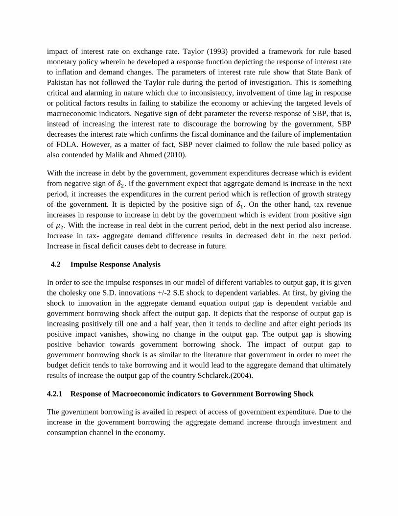
The impulse responses of government borrowing to its self is showing the reverse relationship,

as any shock to government borrowing would be responsible for deterioration to government

borrowing. Before shock, the government borrowing is positive and start with decreasing return

very promptly for first two periods and then it shows a constant decrease for next three periods

and finally reaches at the steady state level.

-.02

-.01

.00

.01

.02

2 4 6 8 10

Figure 7: Response of Government Borrowings to Borrowing Shock

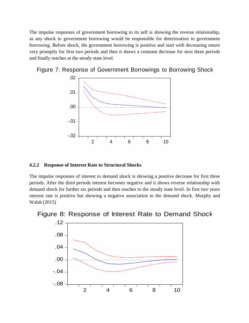
4.2.2 Response of Interest Rate to Structural Shocks

The impulse responses of interest to demand shock is showing a positive decrease for first three

periods. After the third periods interest becomes negative and it shows reverse relationship with

demand shock for further six periods and then reaches to the steady state level. In first two years

interest rate is positive but showing a negative association to the demand shock. Murphy and

Walsh (2015)

-.08

-.04

.00

.04

.08

.12

2 4 6 8 10

Figure 8: Response of Interest Rate to Demand Shock

There is a trade-off between interest rate and inflation, as due to increase in the interest rate the

aggregate dement would shrink and it would lead to decrease in the investment and consumption.

The interest rate to inflation impulse responses showing a constant positive relationship for first

four periods and then it reaches to the steady state level. In the fifth period, the response of

interest rate becomes negative to inflation shock and it moves similarly till ninth periods and

then shows no variation.

-.08

-.04

.00

.04

.08

.12

2 4 6 8 10

Figure 9: Response of Interest Rate to Inflation

The interest rate to risk premium shocks impulse responses are showing a negative association

for first seven periods. The peak of negative association of interest rate to risk premium shock is

at third period and afterward it fosters to the steady state level.

-.08

-.04

.00

.04

.08

.12

2 4 6 8 10

Figure 10: Response of Interest Rate to Risk Premium Shock

The interest rate to interest rate shock is showing a negative association between them. The

impulse responses show that due to the shock in interest rate, the interest rate declines

continuously till fifth periods and then becomes steady state level and instantly goes down to this

level and shows a negative association in the six periods till tenth period.

-.08

-.04

.00

.04

.08

.12

2 4 6 8 10

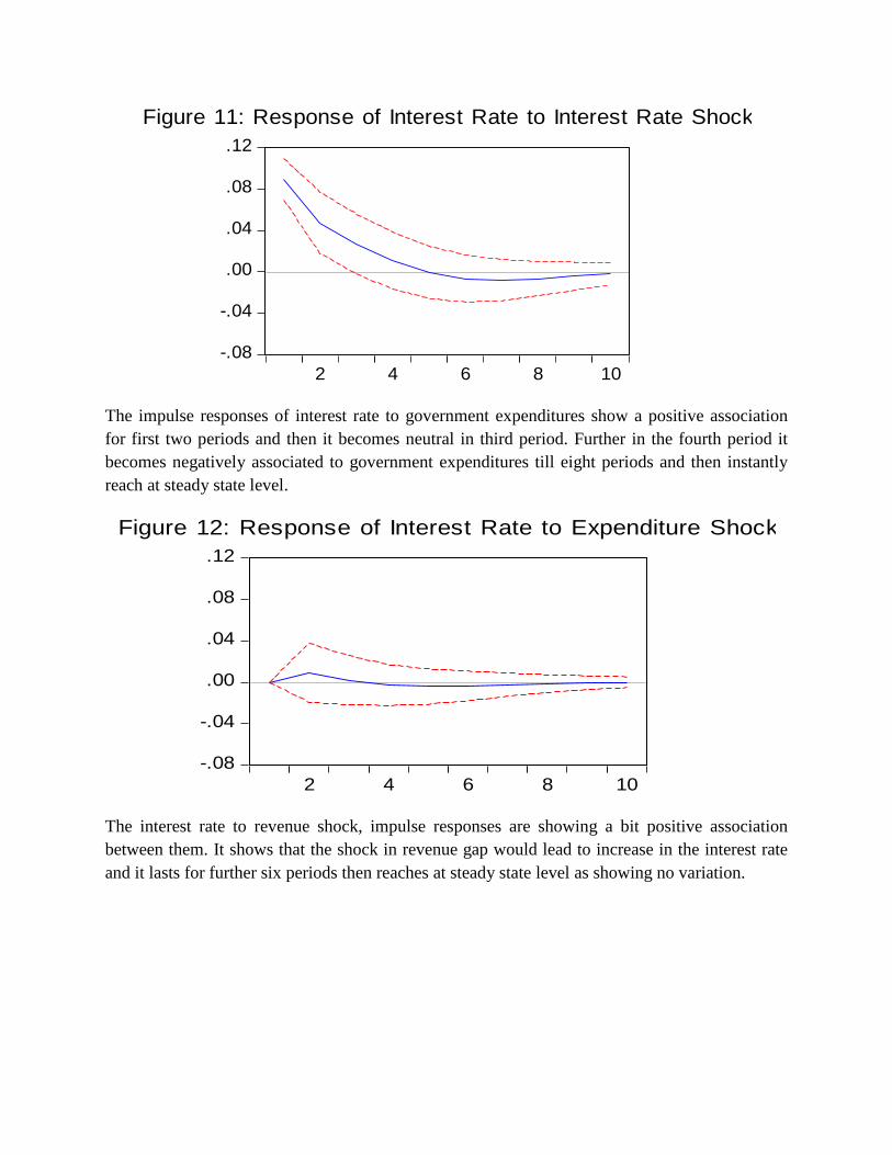
Figure 11: Response of Interest Rate to Interest Rate Shock

The impulse responses of interest rate to government expenditures show a positive association

for first two periods and then it becomes neutral in third period. Further in the fourth period it

becomes negatively associated to government expenditures till eight periods and then instantly

reach at steady state level.

-.08

-.04

.00

.04

.08

.12

2 4 6 8 10

Figure 12: Response of Interest Rate to Expenditure Shock

The interest rate to revenue shock, impulse responses are showing a bit positive association

between them. It shows that the shock in revenue gap would lead to increase in the interest rate

and it lasts for further six periods then reaches at steady state level as showing no variation.

-.08

-.04

.00

.04

.08

.12

2 4 6 8 10

Figure 13: Response of Interest Rate to Revenue Shock

4.6 Generalized Forecast Error Variance Decomposition Analysis

In table 4.6, it can be observed that government borrowing is main contributor for variation in

output gap. Which is almost 10.02% for up to 6 years. It is very important to notice that with the

government borrowings government borrowing is increase but demand will be increased. As a

result of this shock output remain above steady state for almost 2 years. Then it tends to decline

and after eight periods its positive impact vanishes. Risk premium is the second biggest

contributor of accounting 6.73% of the forecast error variance. After that we can also see that

risk premium and inflations are showing 7.47% and 6.73 respectively.

Table 4.6 Variance Decomposition of Output Gap (X):

Period S.E. X INF Q R GGAP TGAP BGAP

1 0.01476 100 0 0 0 0 0 0

2 0.01702 84.138 5.79791 0.0898 3.74269 0.57884 1.90392 3.74887

3 0.01841 72.4905 6.73067 1.97063 7.77472 0.78689 2.85979 7.38682

4 0.01927 66.2103 6.23904 4.64293 9.68921 0.84785 3.1101 9.26057

5 0.01973 63.3629 6.01364 6.55756 10.1907 0.85579 3.11208 9.90735

6 0.01993 62.3026 6.08241 7.47096 10.1926 0.85004 3.07316 10.0282

Table 4.7 shows comparative significance of the structural shocks in describing inflation in

Pakistan. The results show that in the short run output gap is most important for the explaining

variations in inflation. An increase in output gap causes inflation to fall immediately below

steady state level which is unable to recover till 6th

period. It can be also seen that government

borrowing explaining 3.81 % variation in inflation. When there is an increase in government

borrowings money supply will also increase and it will create inflationary pressure in the

economy.

Table 4.7 Variance Decomposition of INF:

Period S.E. X INF Q R GGAP TGAP BGAP

1 1.07643 3.10E-05 100 0 0 0 0 0

2 1.19935 4.62976 85.8065 5.04451 0.71837 0.91034 0.04902 2.8415

3 1.25082 7.54628 79.3485 7.50506 0.66346 1.0968 0.04509 3.79485

4 1.27154 8.44283 78.0927 7.55187 0.95292 1.09898 0.08499 3.77576

5 1.28001 8.4996 77.6621 7.52929 1.31359 1.08684 0.16061 3.74796

6 1.28522 8.43079 77.1262 7.83171 1.49523 1.07813 0.22063 3.81731

Above table is showing the variance decomposition of government borrowing it shows the

variation in borrowing is mostly explain by government borrowing which means that with

increase in government borrowing the will be variation in government borrowing almost 6 to 8

years are needed to get back on steady state level. After government borrowings, risk premium

shock is major source of explanation for variation in government borrowings

Table 4.8 Variance Decomposition of BGAP:

Period S.E. X INF Q R GGAP TGAP BGAP

1 0.02047 3.52109 0.92025 43.6725 0.77016 0.16989 0.11639 50.8298

2 0.02676 10.9236 0.54692 44.2354 4.30636 3.64686 0.07438 36.2665

3 0.0305 14.4735 1.54402 38.9719 10.3267 5.50474 0.06803 29.1111

4 0.03253 14.9726 2.83849 34.4246 15.6942 6.00399 0.0598 26.0063

5 0.03359 14.3633 3.32895 32.8498 18.7761 5.97402 0.06327 24.6446

6 0.03418 13.8799 3.29781 33.1923 19.7768 5.82516 0.07118 23.9569

5. CONCLUSION AND POLICY RECOMENDATIONS

Like other developing countries, Pakistan is also facing the problem of government borrowing.

To pay this debt government have to borrow from available sources (internal source or external

source). In order to access the effect of government borrowings on macroeconomic stability the

model developed in this study taking into account the perspective of New Keynesian Model. It is

very important for policy maker to make policy according to expectations of economic agents.

Because policy responses under the given situation of debt are not as per objectives of policies.

All the parameters, except , , representing the impact of output gap on inflation, interest

rate and government expenditures respectively, have significantly different from zero. In the

Aggregate Demand equation where the dependent variable is output gap, showing the

negative impact of real interest rate [ ] on output gap, reflect that with the decrease in

real interest rate, output gap (or the aggregate demand) increases. shows the elasticity of

household’s intertemporal substitution in consumption and its absolute value is not greater than

zero (Gali and Gertler, 2007). The results of estimates of parameters show the expenditure led

growth in the economy which show the positive influence of fiscal policy but monetary policy

seems to be ineffective to meet the targets set by the fiscal authority.

To analyze the dynamic response of macroeconomic variable to government borrowings

estimation results are derived using maximum likelihood estimation procedure through Structural

Auto Regressive (SVAR) Model. Problem of interpreting VARs is solved with the SVARs by

including restrictions sufficient to identifying the underlying shocks. The results of SVAR is

shown that government borrowing has negative effect on economy.

The dominant role of fiscal authority can be a point of criticism up to extent that there must be

independence of the monetary authority on one hand and there should be some defined

framework of the monetary policy. An appropriate framework that can be built through some

sort of Taylor type rule is necessary. Further to it, an effective monetary-fiscal coordination

effort is need of the time that may also ensure the applicability of FDLA in its true spirit. Debts

are normally treated as necessary phenomenon for the developing economies but the expenditure

preferences and the revenue optimality are necessary ingredients which seems to be missing in

Pakistan during the period of investigation.

References

Auerbach, Alan J., and Laurence J. Kotlikoff, (1987). Dynamic Fiscal Policy. Cambridge:

Cambridge University Press.

Ball, L., (1999). Policy rules for open economies, in J. Taylor (ed.), Monetary Policy Rules.

University of Chicago Press. pp. 127–144.

Calvo, G.A., 1983. Staggered Prices in a Utility-Maximizing Framework. Journal of Monetary

Economics, 12, pp.383–98.

Cebi. C. (2012). The Interaction between Monetary and Fiscal Policies in Turkey: An estimated

New Keynesian DSGE model. Economic Modeling, 29: 1258 – 1267.

Clarida, R., Galí, J., and Gertler, M., 2001. A simple framework for international monetary

policy analysis, NBER Working Paper 8870

Feldstein, Martin, (1995). Budget Deficits and Debt: Issues and Options. Overview Panelist,

Federal Reserve Bank of Kansas City, 403-412.

Galí, J., & Monacelli, T., 2005. Optimal Monetary and Fiscal Policy in a Currency Union, CEPR

Discussion Papers 5374

Gali, Jordi, 1999. Technology, employment, and the business cycle: do technology shocks

explain aggregate fluctuations?," American Economic Review 89(1), 249-271.

Johansen, Søren (1991). "Estimation and Hypothesis Testing of Cointegration Vectors in

Gaussian Vector Autoregressive Models". Econometrica. 59 (6): 1551–1580.

Keating, J., (1990). Identifying VAR models under rational expectations. Journal of Monetary

Economics, 25, pp.453–476.

King, Robert G., Plosser, Charles I. and Rebelo, Sergio T., (1988). Production, Growth, and

Business Cycles: II. New Directions. Journal of Monetary Economics, 21, 309-42.

Kydland, F.E., & Prescott, E.C., (1982). Time to Build and Aggregate

Fluctuations, Econometrica, Econometric Society, 50(6), pp. 1345-70.

Leu, Shawn Chen-Yu, 2011. "A New Keynesian SVAR model of the Australian

economy," Economic Modelling, Elsevier, 28(1), pages 157-168.

McCallum, B. T., (1994). A reconsideration of the uncovered interest parity relationship. Journal

of Monetary Economics 33: 105–132.

Nawaz and Ahmed (2015), New Keynesian Macroeconomic Model and Monetary Policy of

Pakistan. Pakistan Development Review, 54 (1), 2015.

Sargent, T. J., 1980. Rational expectations and the reconstruction of macroeconomics. Federal

Reserve Bank of Minneapolis, Quarterly Review, Summer.

Sims, C.A., 1992. Interpreting the macroeconomic time series facts: The effects of monetary

policy. European Economic Review, Elsevier, 36(5), pp.975-1000, June.

Sims, C.A., Stock, J.H., & Watson, M.W., 1990. Inference in Linear Time Series Models with

Some Unit Roots, Econometrica, 58, 113-144.

Appendix

Table A-4.2: Unrestricted Cointegration Rank Test (Trace)

Hypothesized Trace 0.05

No. of CE(s) Eigenvalue Statistic Critical Value Prob.**

None * 0.987992 390.0656 125.6154 0.0000

At most 1 * 0.839463 213.1791 95.75366 0.0000

At most 2 * 0.802536 140.0098 69.81889 0.0000

At most 3 * 0.576144 75.12179 47.85613 0.0000

At most 4 * 0.433970 40.78737 29.79707 0.0019

At most 5 * 0.237491 18.02303 15.49471 0.0204

At most 6 * 0.164257 7.177376 3.841466 0.0074

Trace test indicates 7 cointegrating eqn(s) at the 0.05 level

* denotes rejection of the hypothesis at the 0.05 level

**MacKinnon-Haug-Michelis (1999) p-values

Table A-4.3: Unrestricted Cointegration Rank Test (Maximum Eigenvalue)

Hypothesized Max-Eigen 0.05

No. of CE(s) Eigenvalue Statistic Critical Value Prob.**

None * 0.987992 176.8865 46.23142 0.0000

At most 1 * 0.839463 73.16927 40.07757 0.0000

At most 2 * 0.802536 64.88803 33.87687 0.0000

At most 3 * 0.576144 34.33442 27.58434 0.0058

At most 4 * 0.433970 22.76434 21.13162 0.0292

At most 5 0.237491 10.84565 14.26460 0.1621

At most 6 * 0.164257 7.177376 3.841466 0.0074

Max-eigenvalue test indicates 5 cointegrating eqn(s) at the 0.05 level

* denotes rejection of the hypothesis at the 0.05 level

**MacKinnon-Haug-Michelis (1999) p-values