Embed Size (px)
Citation preview

UNIVERSIDADE DE LISBOA
FACULDADE DE CIENCIAS
DEPARTAMENTO DE INFORMATICA
GOSSIP-BASED DATA DISTRIBUTION IN
MOBILE AD HOC NETWORKS
Hugo Alexandre Tavares Miranda
DOUTORAMENTO EM INFORMATICA
(Engenharia Informatica)
2007


UNIVERSIDADE DE LISBOA
FACULDADE DE CIENCIAS
DEPARTAMENTO DE INFORMATICA
GOSSIP-BASED DATA DISTRIBUTION IN
MOBILE AD HOC NETWORKS
Hugo Alexandre Tavares Miranda
DOUTORAMENTO EM INFORMATICA
(Engenharia Informatica)
Tese orientada pelo Prof. Doutor Luıs Eduardo Teixeira Rodrigues
2007


This work was partially supported by the European Science Foundation (ESF) programme
Middleware for Network Eccentric and Mobile Applications (MiNEMA), by project
Probabilistically-Structured Overlay Networks (P-SON), POSC/EIA/60941/2004 and by
project Middleware for Context-aware and Adaptive Systems (MICAS),
POSC/EIA/60692/2004 through Fundacao para a Ciencia e Tecnologia (FCT) and FEDER and
by PRODEP


Resumo Extendido
A tecnologia utilizada nas redes sem fios sofreu avancos significativos, que criaram
as condicoes para o desenvolvimento de uma nova geracao de dispositivos computa-
cionais moveis, como os telefones celulares, os computadores portateis e os assistentes
digitais pessoais. Por sua vez, a popularidade crescente destes dispositivos aumentou
o interesse nas aplicacoes de computacao movel que beneficiam da ubiquidade das
redes de computadores.
Os dispositivos computacionais portateis sao tendencialmente de pequena di-
mensao e leves, abdicando de algumas funcionalidades. Em comparacao com, por
exemplo, os computadores de secretaria, os dispositivos moveis apresentam menor
memoria e poder computacional. Adicionalmente, espera-se que nestes dispositivos
ocorram frequentemente interrupcoes temporarias do acesso a rede, devido por exem-
plo a exaustao das baterias, ao deslocamento do dispositivo para uma zona onde nao
existe cobertura ou, simplesmente, porque o utilizador o solicitou.
As redes ad hoc moveis (MANETs, do ingles Mobile Ad hoc NETworks) sao uma
classe particular de redes sem fios caracterizadas pela ausencia de infra-estrutura. Nas
MANETs, a rede e exclusivamente composta pelos dispositivos participantes. Espera-
se que estas redes venham a ser particularmente uteis para situacoes onde a instalacao
da infra-estrutura e excessivamente cara, demorada ou inadequada, por exemplo em
locais afectados por catastrofes naturais, missoes de busca e salvamento ou missoes
militares.
O desenvolvimento de aplicacoes para MANETs tem desafios muito particulares.

Ao contrario do que e comum nas redes fixas e nas redes sem fios infra-estruturadas,
nao e possıvel concentrar servicos como o armazenamento de dados, servico de no-
mes, etc. em servidores especializados e com um elevado grau de fiabilidade. Pelo
contrario, emMANETs estes servicos terao que ser conseguidos atraves da cooperacao
dos participantes. Um exemplo paradigmatico e o encaminhamento de mensagens en-
tre dispositivos e que e suportado por uma cadeia de dispositivos localizados entre
ambos.
Nos ultimos anos foram propostas diversas solucoes para o problema do enca-
minhamento de mensagens. Com este problema resolvido, e agora o momento de
abordar e resolver outras limitacoes ao desenvolvimento de aplicacoes para MANETs.
Idealmente, as solucoes devem ser desenvolvidas sob a forma de camadas de codigo
intermedio, capazes de esconder das aplicacoes as dificuldades que estas redes acarre-
tam.
A disseminacao de dados e um dos servicos chave em MANETs. Este servico per-
mite por exemplo a equipas de busca e salvamento partilhar fotografias ou informacao
actualizada da zona afectada; a passageiros num aeroporto encontrar um parceiro para
um jogo de xadrez ou a vendedores numa feira usar uma MANET para anunciar os
seus produtos. Todos estes exemplos partilham um modelo comum de dados: os da-
dos sao produzidos por diferentes participantes e nao sao actualizados com frequencia.
Alem disso, nao e possıvel inferir um destinatario para os dados nem quais os dispo-
sitivos que estarao mais interessados.
Em MANETs, a concentracao de dados num unico dispositivo deve ser evitada
devido: i) a baixa disponibilidade dos dispositivos; ii) a sobrecarga dos dispositi-
vos que armazenariam os dados e iii) a mobilidade dos dispositivos, que resulta em
interrupcoes frequentes da ligacao a rede e na ocorrencia de particoes. A disponibili-
dade dos dados aumentaria se estes fossem replicados pelos participantes. Por outro
lado, um algoritmo de distribuicao das replicas tem que evitar a redundancia exces-
siva, uma vez que os dispositivos podem ter recursos limitados. Atendendo a que para
os dispositivos que operam nas redes sem fios, quer a largura de banda quer a energia

sao recursos escassos, o algoritmo deve tambem reduzir tanto quanto possıvel a quan-
tidade de dados e informacao de controlo necessaria para proceder a disseminacao.
Nas MANETs, as replicas devem ser distribuıdas de forma uniforme pelos dis-
positivos que formam a rede, evitando a sua agregacao em regioes geograficas. Ou
seja, quando um item de dados e solicitado por um dispositivo, a distancia ao dispo-
sitivo que fornece a informacao deve ser aproximadamente a mesma, independente-
mente da localizacao de ambos. Naturalmente, a distancia real dependera demultiplos
parametros, como o numero de dispositivos, a memoria disponibilizada por cada um
e o numero de itens anunciados.
A distribuicao geografica das replicas pode oferecer uma contribuicao valiosa para
o desempenho das aplicacoes. A transmissao e recepcao de dados contribuem signifi-
cativamente para o consumo de energia dos dispositivos. Se as replicas se encontrarem
distribuıdas geograficamente, um dispositivo que pretenda obter um qualquer item
de dados encontra-lo-a com grande probabilidade num qualquer dispositivo proximo,
permitindo a sua obtencao com umnumeromenor de transmissoes. Contribui-se desta
forma para a reducao do consumo de energia, da latencia na obtencao de informacao
e da quantidade de trafego gerado.
A disseminacao de dados em MANETs, e em particular, a sua distribuicao ge-
ografica, sao problemas que ja foram abordados por diversos grupos de investigacao.
Contudo, a maioria do trabalho anterior assume que os dispositivos conhecem a sua
localizacao geografica. De notar que esta informacao pode nao estar disponıvel, como
por exemplo no interior de edifıcios, mesmo assumindo que os dispositivos moveis
dispoem de equipamentos de localizacao geografica (por exemplo receptores do sis-
tema de posicionamento global, GPS). Este requisito diminui por isso consideravel-
mente o domınio de aplicacao destes algoritmos.
A tese apresenta um conjunto de algoritmos que se complementam para oferecer
um servico integral de replicacao dos dados por um subconjunto, geograficamente
disperso, dos participantes na rede. Assumimos contudo que os dispositivos nao sao
capazes de obter a sua localizacao geografica ou que a informacao disponıvel nao apre-

senta precisao suficiente. A distribuicao geografica permite que os dispositivos ob-
tenham a informacao utilizando um numero limitado de transmissoes, contribuindo
desta forma para a preservacao dos recursos da rede.
As principais contribuicoes da tese sao:
• um novo metodo para a seleccao dos dispositivos mais adequados para proceder
a retransmissao de mensagens que se pretendem difundidas por todos os partici-
pantes. Ometodo utiliza a forca do sinal recebido para seleccionar os dispositivos
mais distantes dos emissores anteriores;
• Um algoritmo de replicacao de dados para MANETs. O algoritmo dispoe as
replicas por forma a que qualquer dispositivo possa encontrar uma replica dos
dados dentro de um numero predefinido de saltos;
• Quatro algoritmos para atenuar o impacto do movimento dos dispositivos na
distribuicao geografica. Estes algoritmos apresentam um consumo diminuto de
recursos, beneficiando do trafego gerado pelas operacoes de obtencao de dados
para avaliar a qualidade da disseminacao e aplicar as correccoes;
• Um algoritmo de agregacao de dados a partir de uma condicao especificada pelo
utilizador e que deve ser satisfeita pelos dados a obter.
A tese comeca por motivar o problema e explanar os requisitos do modelo no
Capıtulo 1. O Capıtulo 2 apresenta o trabalho relacionado, dividido em dois blocos
principais: algoritmos de disseminacao de mensagens e algoritmos de distribuicao de
dados. As contribuicoes da tese para cada um destes aspectos sao apresentadas e ava-
liadas respectivamente nos Capıtulos 3 e 4. Este ultimo apresenta e avalia ainda os
algoritmos de atenuacao do movimento dos dispositivos. O Capıtulo 5 expoe uma
aplicacao dos algoritmos a uma versao do Session Initiation Protocol (SIP) especial-
mente desenvolvida para MANETs. As principais conclusoes deste trabalho assim
como as perspectivas para o trabalho futuro sao apresentadas no Capıtulo 6.

Abstract
Wireless networks are useful in many different scenarios. They allow to create
emergency networks for catastrophe response, wide area surveillance networks in hos-
tile environments, or simply permit users to share information, play on-line games,
and surf the Web. Mobile ad hoc networks are a particular case of wireless networks
characterised by the absence of a supporting infrastructure.
The thesis addresses the problem of building middleware services that permit to
fully exploit the opportunities offered by mobile ad hoc networks. For that purpose, it
is required to design algorithms that account for the limitations of mobile devices and
that make a careful use of the scarce resources available in ad hoc networks. A central
middleware service for mobile applications is data sharing. The thesis addresses the
use of data replication as a technique to improve data availability and resource sav-
ings in mobile ad hoc networks. In particular, the thesis proposes the use of epidemic
protocols to achieve these goals.
In this context, the thesis presents the following contributions. It presents and eval-
uates i) an algorithm to reduce the number of transmissions required in a broadcast,
ii) an algorithms for the geographical distribution of replicas of data items, and iii)
algorithms to attenuate the impact of node movement in the geographical distribu-
tion. Finally, the thesis describes an application of the algorithms to build a concrete
application, a version of the Session Initiation Protocol for wireless networks.


Palavras Chave
Redes ad hoc moveis,
Distribuicao geografica de dados,
Algoritmos de disseminacao
Keywords
Mobile ad hoc networks,
Geographical data distribution,
Broadcast algorithms


Agradecimentos
Na realizacao deste trabalho contei com o apoio pessoal e/ou cientıfico de um
conjunto de pessoas e instituicoes sem as quais este trabalho nao teria sido possıvel.
Aproveito por isso para expressar aqui os meus agradecimentos aqueles que mais sig-
nificativamente deram a sua contribuicao.
Ao Goncalo e ao Pedro agradeco a paciencia com que aceitam as minhas ausencias.
A Cristina devo uma parte significativa destes resultados. Pela motivacao que sempre
me transmitiu, pela disponibilidade com que vai assumindomuitas dasminhas tarefas,
abdicando do seu tempo. Sem a sua energia e apoio nao teria sido possıvel a realizacao
deste trabalho.
Nao teria sido possıvel chegar ate aqui se nao tivesse, ao longo dos tempos, sentido
um apoio continuado no prosseguimento dos meus estudos. Agradeco por isso aos
meus pais e irmas a quem dedico genericamente esta tese.
Foram muitas as instituicoes que contribuiram para este trabalho. O programa
MiNEMA, da European Science Foundation (ESF) suportou financeiramente os contac-
tos com a Universidade de Helsınquia. Adicionalmente, tem servido como um forum
que me permitiu enriquecer a minha formacao, criar e fortalecer lacos com outros in-
vestigadores.
Localmente, contei com o apoio institucional do Departamento de Informatica
da Faculdade de Ciencias da Universidade de Lisboa e do Laboratorio de Sistemas
Informaticos de Grande Escala (LaSIGE). A ambos agradeco a disponibilizacao das
condicoes para desenvolver o meu trabalho. Uma palavra especial para os membros

(passados e presentes) do DIALNP, que tem feito deste grupo um excelente ponto de
partilha de ideias, entreajuda e convıvio, contribuindo assim para um ambiente de
estımulo a investigacao. Um agradecimento especial ao Filipe Araujo pelo cuidado
que pos na revisao de parte desta tese.
O Professor Luıs Rodrigues excedeu largamente o papel de orientador cientıfico
da tese. A sua experiencia, permanente disponibilidade, dinamica invejavel e o em-
penho no acompanhamento dos trabalhos dos alunos e em proporcionar-lhes todas as
condicoes necessarias, sao por si so um dos mais importantes factores de motivacao
e fazem dele um modelo a seguir. Por fim, agradeco-lhe a oportunidade que me
deu de alargar a minha formacao para domınios nao estritamente relacionados com
a elaboracao da tese. Estou certo que experiencias como a organizacao de eventos,
a participacao na elaboracao de propostas de financiamento e em comissoes de pro-
grama, e o estabelecimento de contactos com outros investigadores serao tambem fac-
tores importantes para o desenvolvimento da minha carreira.
Lisboa, Junho de 2007
Hugo Alexandre Miranda

A Cristina
Ao Goncalo e ao Pedro


Contents
Contents i
List of Figures vii
List of Tables xiii
1 Introduction 1
1.1 Problem Statement and Objectives . . . . . . . . . . . . . . . . . . . . . . 3
1.2 Contributions . . . . . . . . . . . . . . . . . . . . . . . . . . . . . . . . . . 4
1.3 Results . . . . . . . . . . . . . . . . . . . . . . . . . . . . . . . . . . . . . . 5
1.4 Outline of the Thesis . . . . . . . . . . . . . . . . . . . . . . . . . . . . . . 5
2 Related Work 9
2.1 General Architecture of Data Distribution Protocols . . . . . . . . . . . . 10
2.2 Local Storage Management . . . . . . . . . . . . . . . . . . . . . . . . . . 11
2.3 Data Dissemination Algorithms . . . . . . . . . . . . . . . . . . . . . . . . 14
2.3.1 Location Unaware Algorithms . . . . . . . . . . . . . . . . . . . . 15
2.3.2 Improved Location Unaware Algorithms . . . . . . . . . . . . . . 20
2.3.3 Trial and Error Algorithms . . . . . . . . . . . . . . . . . . . . . . 24
i

2.3.4 Owner Oriented Algorithms . . . . . . . . . . . . . . . . . . . . . 28
2.3.5 Location Aware Algorithms . . . . . . . . . . . . . . . . . . . . . . 31
2.3.6 Discussion . . . . . . . . . . . . . . . . . . . . . . . . . . . . . . . . 33
2.4 Packet Dissemination . . . . . . . . . . . . . . . . . . . . . . . . . . . . . . 36
2.4.1 Broadcast Algorithms . . . . . . . . . . . . . . . . . . . . . . . . . 37
2.4.2 Probabilistic Algorithms . . . . . . . . . . . . . . . . . . . . . . . . 39
2.4.3 Counter-based Algorithms . . . . . . . . . . . . . . . . . . . . . . 43
2.4.4 Distance-Aware Algorithms . . . . . . . . . . . . . . . . . . . . . . 47
2.4.5 Discussion . . . . . . . . . . . . . . . . . . . . . . . . . . . . . . . . 50
2.5 Summary . . . . . . . . . . . . . . . . . . . . . . . . . . . . . . . . . . . . . 53
3 A Power-Aware Broadcasting Algorithm 57
3.1 Pampa . . . . . . . . . . . . . . . . . . . . . . . . . . . . . . . . . . . . . . 59
3.1.1 Delay Assignment . . . . . . . . . . . . . . . . . . . . . . . . . . . . 61
3.2 Comparison with Related Work . . . . . . . . . . . . . . . . . . . . . . . . 62
3.3 Simulation Results . . . . . . . . . . . . . . . . . . . . . . . . . . . . . . . 63
3.3.1 Test-bed . . . . . . . . . . . . . . . . . . . . . . . . . . . . . . . . . 64
3.3.2 Delivery Ratio . . . . . . . . . . . . . . . . . . . . . . . . . . . . . . 65
3.3.2.1 Impact of the bounded delay . . . . . . . . . . . . . . . . 68
3.3.3 Number of Transmissions . . . . . . . . . . . . . . . . . . . . . . . 70
3.3.4 Coverage . . . . . . . . . . . . . . . . . . . . . . . . . . . . . . . . . 72
3.3.5 Delay . . . . . . . . . . . . . . . . . . . . . . . . . . . . . . . . . . . 73
3.4 Summary . . . . . . . . . . . . . . . . . . . . . . . . . . . . . . . . . . . . . 73
ii

4 Replica Management 75
4.1 System Model . . . . . . . . . . . . . . . . . . . . . . . . . . . . . . . . . . 76
4.2 Initialisation . . . . . . . . . . . . . . . . . . . . . . . . . . . . . . . . . . . 77
4.3 Data Dissemination . . . . . . . . . . . . . . . . . . . . . . . . . . . . . . . 80
4.3.1 Power-Aware data DISsemination algorithm . . . . . . . . . . . . 81
4.3.2 Geographical Distribution of the Replicas . . . . . . . . . . . . . . 84
4.3.2.1 Expected Maximum Distance . . . . . . . . . . . . . . . 87
4.3.2.2 Expected Reply Distance . . . . . . . . . . . . . . . . . . 88
4.3.2.3 Cluster Storage Space and Saturation Point . . . . . . . 89
4.3.3 Decreasing the Impact of the Limited Storage . . . . . . . . . . . . 91
4.3.3.1 Hold period . . . . . . . . . . . . . . . . . . . . . . . . . 92
4.3.3.2 Storage Space Management . . . . . . . . . . . . . . . . 93
4.3.4 Illustration . . . . . . . . . . . . . . . . . . . . . . . . . . . . . . . . 94
4.4 Data Retrieval . . . . . . . . . . . . . . . . . . . . . . . . . . . . . . . . . . 96
4.4.1 Adaptation of the qTTL value . . . . . . . . . . . . . . . . . . . . . 99
4.5 Shuffling . . . . . . . . . . . . . . . . . . . . . . . . . . . . . . . . . . . . . 100
4.5.1 Effects of Movement in Data Placement . . . . . . . . . . . . . . . 101
4.5.2 Herald Messages . . . . . . . . . . . . . . . . . . . . . . . . . . . . 102
4.5.3 Characterisation of Shuffling Algorithms . . . . . . . . . . . . . . 103
4.5.4 Shuffling Algorithms . . . . . . . . . . . . . . . . . . . . . . . . . . 104
4.5.5 Illustration . . . . . . . . . . . . . . . . . . . . . . . . . . . . . . . . 108
4.6 Comparison with Related Work . . . . . . . . . . . . . . . . . . . . . . . . 111
iii
4.7 Evaluation . . . . . . . . . . . . . . . . . . . . . . . . . . . . . . . . . . . . 113
4.7.1 Dissemination Algorithm . . . . . . . . . . . . . . . . . . . . . . . 114
4.7.1.1 Sensitivity to Different Network Configurations . . . . . 114
4.7.1.2 Message Overhead . . . . . . . . . . . . . . . . . . . . . 119
4.7.1.2.1 Dissemination . . . . . . . . . . . . . . . . . . . 120
4.7.1.2.2 Queries . . . . . . . . . . . . . . . . . . . . . . . 121
4.7.1.3 Attenuation of the Dissemination Cost . . . . . . . . . . 122
4.7.2 Shuffling Algorithms . . . . . . . . . . . . . . . . . . . . . . . . . . 124
4.7.2.1 Probability of Insertion . . . . . . . . . . . . . . . . . . . 128
4.7.2.2 Convergence Tests . . . . . . . . . . . . . . . . . . . . . . 129
4.7.2.3 Mitigation Tests . . . . . . . . . . . . . . . . . . . . . . . 137
4.8 Summary . . . . . . . . . . . . . . . . . . . . . . . . . . . . . . . . . . . . . 145
5 Application 147
5.1 Overview of SIP . . . . . . . . . . . . . . . . . . . . . . . . . . . . . . . . . 148
5.1.1 Decentralised SIP . . . . . . . . . . . . . . . . . . . . . . . . . . . . 150
5.2 SIPCache . . . . . . . . . . . . . . . . . . . . . . . . . . . . . . . . . . . . . 152
5.2.1 Dissemination and Retrieval Using PADIS . . . . . . . . . . . . . 152
5.2.2 Data Gathering Module . . . . . . . . . . . . . . . . . . . . . . . . 154
5.2.2.1 Detailed Description . . . . . . . . . . . . . . . . . . . . 156
5.3 Evaluation . . . . . . . . . . . . . . . . . . . . . . . . . . . . . . . . . . . . 162
5.3.1 Test-bed Description . . . . . . . . . . . . . . . . . . . . . . . . . . 162
5.3.2 Coverage . . . . . . . . . . . . . . . . . . . . . . . . . . . . . . . . . 164
iv

5.3.3 Traffic . . . . . . . . . . . . . . . . . . . . . . . . . . . . . . . . . . 166
5.4 Summary . . . . . . . . . . . . . . . . . . . . . . . . . . . . . . . . . . . . . 171
6 Conclusions and Future Work 173
6.1 Future Work . . . . . . . . . . . . . . . . . . . . . . . . . . . . . . . . . . . 175
References 177
Index 185
v

vi

List of Figures
1.1 Architecture of data distribution middleware frameworks . . . . . . . . 6
2.1 Generic architecture of data distribution protocols . . . . . . . . . . . . . 10
2.2 A taxonomy of data dissemination algorithms . . . . . . . . . . . . . . . 15
2.3 Intersection of trails and queries in rumour routing . . . . . . . . . . . . 17
2.4 Storage and query circles in Double Ruling storage . . . . . . . . . . . . . 26
2.5 Network region partitioning in GLS . . . . . . . . . . . . . . . . . . . . . 28
2.6 Home node and perimeter in Data-Centric Storage . . . . . . . . . . . . . 30
2.7 Monitor nodes in Resilient-Data-Centric Storage . . . . . . . . . . . . . . 32
2.8 Flooding algorithm . . . . . . . . . . . . . . . . . . . . . . . . . . . . . . . 38
2.9 GOSSIP1(p) algorithm . . . . . . . . . . . . . . . . . . . . . . . . . . . . . 39
2.10 GOSSIP1(p, k) algorithm . . . . . . . . . . . . . . . . . . . . . . . . . . . . 41
2.11 GOSSIP2(p1, k, p2, n) algorithm . . . . . . . . . . . . . . . . . . . . . . . . 42
2.12 RAPID algorithm . . . . . . . . . . . . . . . . . . . . . . . . . . . . . . . . 42
2.13 Probability adaptation function in RAPID . . . . . . . . . . . . . . . . . . 43
2.14 Enhanced RAPID algorithm . . . . . . . . . . . . . . . . . . . . . . . . . . 44
2.15 GOSSIP3(p, k,m) algorithm . . . . . . . . . . . . . . . . . . . . . . . . . . 45
vii

2.16 Counter-based scheme . . . . . . . . . . . . . . . . . . . . . . . . . . . . . 46
2.17 Hop Count-Aided Broadcasting algorithm . . . . . . . . . . . . . . . . . 47
2.18 Overlap of the coverage between two nodes . . . . . . . . . . . . . . . . . 48
2.19 Distance-based scheme . . . . . . . . . . . . . . . . . . . . . . . . . . . . . 49
2.20 Self-Adaptive Probability Broadcasting Algorithm . . . . . . . . . . . . . 51
3.1 Deployment and transmission range of some nodes . . . . . . . . . . . . 58
3.2 Pampa algorithm . . . . . . . . . . . . . . . . . . . . . . . . . . . . . . . . 60
3.3 Function delay . . . . . . . . . . . . . . . . . . . . . . . . . . . . . . . . . . 62
3.4 Delivery Ratio of Counter Based algorithms . . . . . . . . . . . . . . . . . 66
3.5 Delivery Ratio of Distance Based algorithms . . . . . . . . . . . . . . . . 68
3.6 Comparison of the delivery ratio of Pampa with the “counter-based
scheme” . . . . . . . . . . . . . . . . . . . . . . . . . . . . . . . . . . . . . 69
3.7 Comparison of the delivery ratio of Pampa with Pampa2. . . . . . . . . 70
3.8 Transmissions ratio . . . . . . . . . . . . . . . . . . . . . . . . . . . . . . . 71
3.9 Hops to the source of the message (Speed 0) . . . . . . . . . . . . . . . . . 72
3.10 Average latency (Speed 0) . . . . . . . . . . . . . . . . . . . . . . . . . . . 73
4.1 Initialisation procedure of the algorithms . . . . . . . . . . . . . . . . . . 78
4.2 Auxiliary modules of the distribution and query algorithms . . . . . . . 79
4.3 Example of dissemination of an item . . . . . . . . . . . . . . . . . . . . . 81
4.4 Data dissemination algorithm . . . . . . . . . . . . . . . . . . . . . . . . . 83
4.5 Recursive reverse shortest path to a replica . . . . . . . . . . . . . . . . . 86
4.6 An example of data propagation in the algorithm. . . . . . . . . . . . . . 87
viii

4.7 Counter-examples to the general expected distance rule . . . . . . . . . . 87
4.8 Partitioning of the cluster in rings for DbC=4 . . . . . . . . . . . . . . . . 88
4.9 Function τ(DbC) . . . . . . . . . . . . . . . . . . . . . . . . . . . . . . . . 90
4.10 A run of the dissemination algorithm . . . . . . . . . . . . . . . . . . . . 95
4.11 Retrieval algorithm - sender . . . . . . . . . . . . . . . . . . . . . . . . . . 97
4.12 Retrieval algorithm - query handling . . . . . . . . . . . . . . . . . . . . . 98
4.13 Retrieval algorithm - replies handling . . . . . . . . . . . . . . . . . . . . 99
4.14 Effects of movement in the distribution of the replicas . . . . . . . . . . . 102
4.15 Format of HERALD message tuples . . . . . . . . . . . . . . . . . . . . . . 103
4.16 Swap of data items between two nodes storage spaces . . . . . . . . . . . 105
4.17 Distance evaluation of a worst case scenario simulation . . . . . . . . . . 108
4.18 Variation of the standard deviation of the number of copies . . . . . . . . 110
4.19 Average distance of the replies . . . . . . . . . . . . . . . . . . . . . . . . 116
4.20 Average distance of the replies with variation of number of advertised
items . . . . . . . . . . . . . . . . . . . . . . . . . . . . . . . . . . . . . . . 120
4.21 Transmissions per registration . . . . . . . . . . . . . . . . . . . . . . . . . 120
4.22 Transmissions per query . . . . . . . . . . . . . . . . . . . . . . . . . . . . 122
4.23 Ratio of transmissions per query/transmissions per registration . . . . . 123
4.24 Snapshot of the Manhattan Grid movement model with 7 by 3 streets . . 125
4.25 Average distance of the nodes to the closest replica for two configura-
tions of the Probabilistic algorithm . . . . . . . . . . . . . . . . . . . . . . 130
4.26 Convergence tests when DbC=2 and transmission range=200m . . . . . . 131
4.27 Convergence tests when DbC=2 and transmission range=250m . . . . . . 132
ix

4.28 Convergence tests when DbC=2 and transmission range=300m . . . . . . 133
4.29 Convergence tests when DbC=4 and transmission range=200m . . . . . . 134
4.30 Mitigation tests with 200m transmission range, 2m/s average speed, 700
items and DbC=4 . . . . . . . . . . . . . . . . . . . . . . . . . . . . . . . . 137
4.31 Mitigation tests with 200m transmission range, 2m/s average speed, 400
items and DbC=2 . . . . . . . . . . . . . . . . . . . . . . . . . . . . . . . . 138
4.32 Mitigation tests with 250m transmission range, 2m/s average speed, 700
items and DbC=2 . . . . . . . . . . . . . . . . . . . . . . . . . . . . . . . . 139
4.33 Mitigation tests with 200m transmission range, 2m/s average speed, 700
items and DbC=2 . . . . . . . . . . . . . . . . . . . . . . . . . . . . . . . . 140
4.34 Mitigation tests with 200m transmission range, 5m/s average speed, 700
items and DbC=4 . . . . . . . . . . . . . . . . . . . . . . . . . . . . . . . . 141
4.35 Mitigation tests with 200m transmission range, 5m/s average speed, 400
items and DbC=2 . . . . . . . . . . . . . . . . . . . . . . . . . . . . . . . . 142
4.36 Mitigation tests with 250m transmission range, 5m/s average speed, 700
items and DbC=2 . . . . . . . . . . . . . . . . . . . . . . . . . . . . . . . . 143
4.37 Mitigation tests with 200m transmission range, 5m/s average speed, 700
items and DbC=2 . . . . . . . . . . . . . . . . . . . . . . . . . . . . . . . . 144
5.1 Simplified logical message flow in SIP . . . . . . . . . . . . . . . . . . . . 149
5.2 Software architecture for decentralised SIP . . . . . . . . . . . . . . . . . 150
5.3 Simplified logical message flow in dSIP . . . . . . . . . . . . . . . . . . . 151
5.4 Software architecture for SIPCache . . . . . . . . . . . . . . . . . . . . . . 153
5.5 Simplified logical message flow in SIPCache . . . . . . . . . . . . . . . . 154
5.6 Binding dissemination in SIPCache . . . . . . . . . . . . . . . . . . . . . . 154
x

5.7 Query handling in SIPCache . . . . . . . . . . . . . . . . . . . . . . . . . . 155
5.8 Propagation of gathering messages and replies . . . . . . . . . . . . . . . 157
5.9 Bootstrap of the data gathering operation . . . . . . . . . . . . . . . . . . 158
5.10 Policies for filling data gathering messages with known data items . . . 159
5.11 Data Gathering message dissemination . . . . . . . . . . . . . . . . . . . 161
5.12 Reply handling . . . . . . . . . . . . . . . . . . . . . . . . . . . . . . . . . 162
5.13 Auxiliary functions . . . . . . . . . . . . . . . . . . . . . . . . . . . . . . . 163
5.14 Coverage of the data gathering module . . . . . . . . . . . . . . . . . . . 165
5.15 Retransmissions of the gathering message . . . . . . . . . . . . . . . . . . 166
5.16 Average data gathering message size . . . . . . . . . . . . . . . . . . . . . 167
5.17 Average number of reply messages . . . . . . . . . . . . . . . . . . . . . . 168
5.18 Average bytes per operation . . . . . . . . . . . . . . . . . . . . . . . . . . 170
xi

xii

List of Tables
2.1 Comparison of the data dissemination algorithms surveyed . . . . . . . 34
2.2 Comparison of the broadcast algorithms surveyed . . . . . . . . . . . . . 52
3.1 Comparison of the broadcast algorithms surveyed with Pampa . . . . . 63
4.1 Comparison of the characteristics of the shuffling algorithms . . . . . . . 105
4.2 Comparison of the data dissemination algorithms surveyed with PADIS 112
4.3 Saturation Point Ratios for Convergence tests . . . . . . . . . . . . . . . . 126
4.4 Saturation Point Ratios for Mitigation tests . . . . . . . . . . . . . . . . . 127
5.1 Proportion of the reply messages and total bytes per operation transmit-
ted by the “Not Filled” policy sent by the “Random” policy . . . . . . . . 169
xiii

xiv
1Introduction
Advances in wireless network technology paved the way to the development of a
new generation of communication devices, like cell phones, wireless enabled laptops
and PDAs. The growing popularity of these devices has increased the demand for
mobile computing applications that can benefit from ubiquitous connectivity.
A common requirement for wireless devices is that they should be portable, so that
they can be easily carried by the users. Therefore, mobile devices tend to be small and
lightweight, trading of some functionalities by size. In comparison with, for example,
desktop computers, mobile devices present lower computing power and less memory.
Mobile devices are expected to be temporarily disconnected, due to drained batteries,
movement of the device to some location outside the network range or simply because
the user has requested it.
Mobile Ad hoc NETworks (MANETs) are one particular class of wireless networks
characterised by the lack of a support infrastructure. The network is composed only by
the mobile devices. MANETs are particularly useful for situations where the deploy-
ment of an infrastructure is expensive or impossible like catastrophe scenarios, search
and rescue, and military operations.
Application development is particularly challenging in MANETs. Contrary to
what is typical in wired or wireless infrastructured networks, it is not possible to cen-
tralise in some reliable and powerful server functions such as data storage, naming
service, etc. Instead, these services must be provided via the cooperation of the par-
ticipating devices. A notorious example is packet routing between two devices not in
1

2 CHAPTER 1. INTRODUCTION
transmission range, which must be supported by a sequence of intermediate devices
that forward the message.
Packet routing in ad hoc networks has received considerable attention in the last
few years and a number of interesting protocols have been proposed. With the routing
problem solved, it is time to identify and resolve other impairments to the develop-
ment of distributed applications in MANETs. Ideally, solutions should be provided as
middleware services, capable of masking the peculiarities of ad hoc networks to the
application.
Data dissemination is one of the key applications of MANETs. Teams of a search-
and-rescue operation may want to exchange photographs or up-to-date information of
the disaster scene, participants on a digital flea market may use a MANET to advertise
their products, and passengers waiting on an airport may try to find a partner for a
chess game. All these scenarios share a common data model: data is produced by
different nodes and is not frequently updated. Furthermore, there is not an a priori
known target node for consuming the data, nor it is possible to infer which nodes are
more likely to be interested on it.
The concentration of the data in a single node is unsuitable in MANETs due to
i) the low availability of the devices; ii) the overload of the device storing the data;
and iii) the mobility of the devices, which results in frequent network disconnections
and network partitions. Data availability may be improved if multiple replicas are
distributed through the participants. However, a data dissemination algorithm for
MANETs should balance the need to provide data replication with the need to avoid
excessive data redundancy (as nodes may have limited storage capability). Since in
wireless networks both bandwidth and battery power are precious resources, the al-
gorithm should also minimise the amount of data and control packets required to dis-
seminate data.
In MANETs, data replicas should be deployed as evenly as possible among all the
nodes that form the network, avoiding clustering of information in sub-areas. That is,
whenever a data item is requested by a node S, the distance to the node that provides

1.1. PROBLEM STATEMENT AND OBJECTIVES 3
the reply should be approximately the same, regardless of the location of S. Naturally,
the actual distance depends on multiple parameters, such as the number of nodes in
the network, the amount of memorymade available at each node, and the total number
of data items stored in the network.
The geographical distribution of the replicas can provide a valuable contribution
to the performance of the data dissemination applications. Packet transmission and
reception have been identified as some of the most resource demanding operations
for mobile devices (Feeney & Nilsson, 2001). If replicas are geographically distributed,
nodes are more likely to contact at least one of them using a small number of messages,
saving their battery reserves. Because replicas can be found close to any node, the
query time is reduced, what contributes to improve latency and reduce the traffic.
Due to its importance, data dissemination in MANETs has been a subject widely
studied. In particular, the development of data dissemination algorithms that aim at
a geographical distribution of items is not novel. However, most of previous work
assumes that nodes are aware of their geographical location. That is, these algorithms
can only be applied if mobile nodes have some location device available or perform
complex computations to determine their position. In addition, we note that at some
sites (for example indoors), location information may not be available or it may not be
possible to obtain it with sufficient accuracy. Therefore, the application domain of the
existing geographical data distribution algorithms is severely limited.
1.1 Problem Statement and Objectives
The goal of this thesis is to devise algorithms that distribute replicas of data items
by some of the mobile nodes in an ad hoc network. The thesis assumes that nodes are
unable to retrieve their geographical location. Still, replicas should be geographically
distributed so that any node in the network can retrieve the item from a location at
most a few hops away.

4 CHAPTER 1. INTRODUCTION
The thesis assumes that all nodes cooperate to the successful execution of the al-
gorithms. In particular, nodes are required to i) make some storage space available to
be managed by the algorithms; and ii) send all the messages that are required, for ex-
ample, by contributing to the propagation of the messages transmitted by other nodes
and by replying to queries.
An ideal data distribution algorithm should provide consistent updates of the
replicas, high availability and partition tolerance. Unfortunately, Gilbert & Lynch
(2002) have proven the Brewer’s conjecture, which stated that at most two of these
properties can be achieved simultaneously. In this thesis, replicas are used to improve
availability and tolerance to partitions. The lack of consistency support does not nec-
essarily limit the utility of the algorithms: this section has already presented some ex-
amples of applications where data is not frequently updated and which do not depend
of strict consistency requirements for their correct execution.
1.2 Contributions
The main contributions of this thesis are:
• A novel method for the selection of the most adequate nodes for retransmitting
a message in a broadcast. The method uses the Received Signal Strength Indi-
cator (RSSI) to select nodes that are more distant from the source of the previ-
ous retransmissions. The selection criteria improves previous work by requiring
a lower number of retransmissions for delivering the message to a comparable
number of nodes.
• A replication algorithm for mobile ad hoc networks. The algorithm places copies
at a bounded number of hops of any node in the network so that data can be
retrieved with a limited number of messages. In addition, the algorithm presents
a moderate use of the memory of the devices. The algorithm performs these tasks
without using location information.

1.3. RESULTS 5
• Four alternative shuffling algorithms to mitigate the impact of node movement
in the geographical distribution. The algorithms relocate replicas in the back-
ground and use the feedback provided by messages used for other operations.
The algorithms differentiate by the effort to preserve the number of replicas and
by the type of messages they use.
• A data gathering mechanism to retrieve multiple items satisfying some condi-
tion that benefits of the geographical distribution of the replicas to minimise the
number of transmissions.
1.3 Results
The thesis presents the following results:
• A middleware framework for replica distribution in MANETs. The framework
provides services for geographical distribution of the replicas, data retrieval and
shuffling.
• Extensive simulation results that confirm the properties claimed by the frame-
work.
• A proof-of-concept application to a framework that adapts the Session Initiation
Protocol (SIP) to mobile ad hoc networks.
1.4 Outline of the Thesis
In this thesis we present the components of a scalable middleware framework for
data distribution and retrieval in ad hoc networks. The framework replicates data
items so that nodes have one replica located in a bounded and predefined number of
hops. A general overview of the framework is presented in Figure 1.1. The framework

6 CHAPTER 1. INTRODUCTION
DisseminationRetrieval Shuffling
Data Management
Packet Dissemination
Application
Chapter 4
Chapter 3
Chapter 5
Data Distribution Middleware
Figure 1.1: Architecture of data distribution middleware frameworks
is composed by a Data Management and a Packet Dissemination module. The chapter
where each of the components is described is presented on the right.
The thesis is structured as follows. Chapter 2 presents a survey of the related work.
Our work combines a novel broadcast algorithm with data management algorithms.
Previously, these aspects have been addressed has two independent lines of research.
The chapter reflects this separation by presenting two major sections, each covering
some of the most significant contributions to the state of the art on these research
trends. Each section is concluded with a comparison of the algorithms surveyed and
an analysis focused on their limitations, which is used to motivate our work.
The broadcast algorithm is the focus of Chapter 3. The chapter begins with the
description of the algorithm, named“Pampa”, and then proceeds to compare it both
analytically and by the results of simulations with some of the related work.
Chapter 4 addresses the data management module. The chapter starts with a de-
scription of the dissemination, query and shuffling algorithms. The quality of the dis-
semination and the capability of the shuffling algorithms to keep an acceptable data
distribution in spite of node movement are evaluated in separate in the second part of
the chapter.
1.4. OUTLINE OF THE THESIS 7
The framework was integrated in an independent project aiming to adapt the Ses-
sion Initiation Protocol (SIP) to ad hoc networks. An overview of the project and of
the contribution of the algorithms described in the thesis is presented in Chapter 5.
The chapter also describes and evaluates the data gathering module of the project, that
benefits of the dissemination capabilities of the framework to retrieve the data items
satisfying some condition.
The most significant conclusions of the thesis and some directions for the continu-
ation of this work are presented in Chapter 6.
Related Publications
Preliminary versions of portions of this dissertation have been published in the
following:
• MIRANDA, HUGO, LEGGIO, SIMONE, RODRIGUES, LUIS, & RAATIKAINEN,
KIMMO. 2006a (Sept. 11–14). A power-aware broadcasting algorithm. In: Pro-
ceedings of the 17th Annual IEEE International Symposium on Personal, Indoor and
Mobile Radio Communications (PIMRC’06). University of Oulu, Helsinki, Finland.
This paper presents the Power-AwareMessage PropagationAlgorithm (PAMPA).
The performance of PAMPA is estimated using a network simulator and com-
pared with other message propagation algorithms.
• MIRANDA, HUGO, LEGGIO, SIMONE, RODRIGUES, LUIS, & RAATIKAINEN,
KIMMO. 2006b (Dec. 12–15). An algorithm for distributing and retrieving in-
formation in sensor networks. Pages 31–45 of: Proceedings of the 10th International
Conference on Principles of Distributed Systems (OPODIS 2006) - part II - Brief An-
nouncements.
This brief announcement paper presents and evaluates a preliminary version of
Power-Aware data DISsemination algorithm (PADIS), the data dissemination al-
gorithm described in the dissertation.

8 CHAPTER 1. INTRODUCTION
• MIRANDA, HUGO, LEGGIO, SIMONE, RODRIGUES, LUIS, & RAATIKAINEN,
KIMMO. 2007 (Aug. 28–31). An algorithm for dissemination and retrieval of
information in wireless ad hoc networks. Proceedings of the 13th International Euro-
Par Conference - European Conference on Parallel and Distributed Computing. Lecture
Notes in Computer Science. Rennes, France: Springer. (to appear).
The most up-to-date version of PADIS is described in this paper. The perfor-
mance of PADIS is estimated by varying multiple parameters using a network
simulator.
• MIRANDA, HUGO, LEGGIO, SIMONE, RODRIGUES, LUIS, & RAATIKAINEN,
KIMMO. 2006c. Global data management. Emerging Communication: Studies in
New Technologies and Practices in Communication, vol. 8. Nieuwe Hemweg
6B, 1013 BG Amsterdam, The Netherlands: IOS Press. Chap. Epidemic Dissemi-
nation for Probabilistic Data Storage, pages 124–145.
This book chapter begins with a characterisation and overview of recent results
on gossip protocols. It then proceeds to describe and evaluate a preliminary ver-
sion of PADIS named PCache and the data gatheringmechanism that is presented
in this dissertation.
• LEGGIO, SIMONE, MIRANDA, HUGO, RAATIKAINEN, KIMMO, & RODRIGUES,
LUIS. 2006 (July 17–21). SIPCache: A distributed SIP location service for mo-
bile ad-hoc networks. In: Proceedings of the 3rd Annual International Conference on
Mobile and Ubiquitous Systems: Networks and Services (MOBIQUITOUS 2006).
This short paper presents SIPCache, a Session Initiation Protocol (SIP) for ad hoc
networks. The paper focus on the integration of the three components that result
in SIPCache: dSIP, PADIS and the data gathering mechanism.

2Related Work
The frequent disconnections, low reliability and limited resources of mobile de-
vices make efficient data dissemination and data retrieval challenging problems in
wireless networks. This chapter surveys research results on data dissemination pro-
tocols.
Wireless networks can be applied on a multitude of application scenarios, each
characterised by different data access patterns and device capabilities. The chapter
reflects this heterogeneity by surveying data dissemination protocols for sensor, infra-
structured, hybrid and ad hoc networks. The goal is to identify approaches that, inde-
pendently of the original application scenario, can be applied in MANETs. In addition,
from the survey will emerge an interesting and useful approach for MANETs which,
to the extent of our knowledge, has not been attempted before and will be the focus of
the thesis.
This chapter is organised as follows. Section 2.1 identifies themost relevant compo-
nents of a generic data replication service. Related work on these components, namely
local storage management, data distribution and packet dissemination is presented re-
spectively from Section 2.2 to Section 2.4. Themost relevant conclusions extracted from
the survey are summarised on Section 2.5.
9
10 CHAPTER 2. RELATEDWORK
Local Storage
Packet Dissemination
Data Management
Data Retrieval
Data Dissemination Replica Refreshment
Replica Location
Figure 2.1: Generic architecture of data distribution protocols
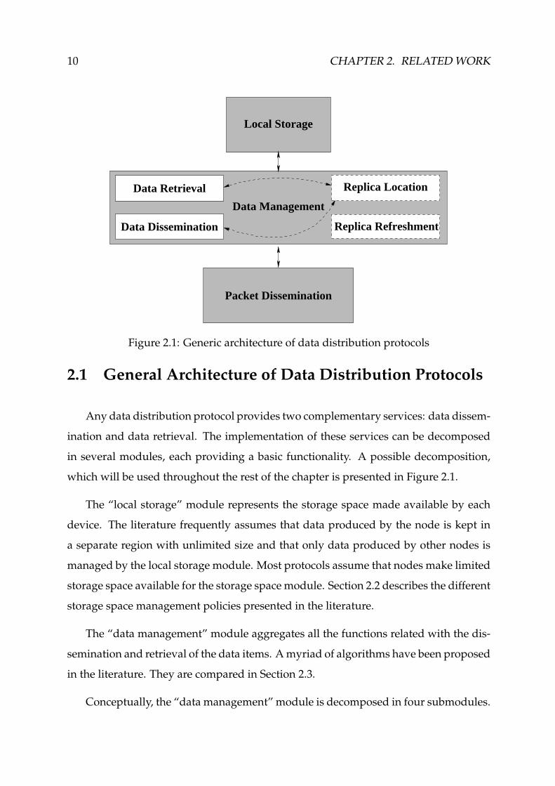
2.1 General Architecture of Data Distribution Protocols
Any data distribution protocol provides two complementary services: data dissem-
ination and data retrieval. The implementation of these services can be decomposed
in several modules, each providing a basic functionality. A possible decomposition,
which will be used throughout the rest of the chapter is presented in Figure 2.1.
The “local storage” module represents the storage space made available by each
device. The literature frequently assumes that data produced by the node is kept in
a separate region with unlimited size and that only data produced by other nodes is
managed by the local storage module. Most protocols assume that nodes make limited
storage space available for the storage space module. Section 2.2 describes the different
storage space management policies presented in the literature.
The “data management” module aggregates all the functions related with the dis-
semination and retrieval of the data items. Amyriad of algorithms have been proposed
in the literature. They are compared in Section 2.3.
Conceptually, the “data management” module is decomposed in four submodules.

2.2. LOCAL STORAGE MANAGEMENT 11
The algorithms supporting data replication are provided by the “data dissemination”
submodule. The “replica refreshment” submodule is present only in some of the proto-
cols surveyed. It is responsible for monitoring and correcting either the number or the
location of the replicas. The “data retrieval” submodule issues queries for data items
and collects and prepares replies.
Some protocols apply deterministic functions to decide the location or identity of
the nodes hosting the replicas. We assume that these protocols use a “replica location”
submodule. If available, the “Replica Location” submodule is used by the “data dis-
semination” and “data retrieval” submodules respectively to decide the location of the
replicas and the destination of queries.
Although conceptually independent, the algorithms implemented in the “data dis-
semination”, “data retrieval” and “replica location” modules are typically tightly cou-
pled. For clarity, these modules are aggregated in the description of the related work.
The “packet dissemination” module exports the message reception and dissemi-
nation primitives that interface the underlying network. Depending of the algorithms
implemented in the remaining modules, point-to-point, multicast and broadcast algo-
rithms may be required. Section 2.4 addresses this module, putting particular empha-
sis on broadcast algorithms as they will be one of the building blocks of the algorithms
presented in the thesis.
2.2 Local Storage Management
The “local storage” module manages a device’s storage space made available for
storing replicas of data items advertised by other nodes. When the storage space made
available by a device is full, an algorithm must be applied to decide which data items
should be kept and which should be discarded. This algorithm plays an important
role in the overall performance of data distribution protocols. Local storage manage-
ment has been previously addressed in different settings, such as operating systems,
12 CHAPTER 2. RELATEDWORK
databases and web caching. The Least Recently Used (LRU) algorithm is frequently
cited as an example of a policy offering good performance in different settings. The
literature has also shown that for wireless networks, it is possible to devise specialised
algorithms that provide a better performance than more general solutions.
Two different approaches, specifically addressing the wireless environment have
been proposed, namely: i) algorithms accounting with the popularity of the data ob-
jects aim at reducing the average reply time by keeping the most popular items, so that
queries can be replied faster. ii) Other algorithms privilege data availability, giving
preference to the diversity of the items in the collective storage space defined by the
union of the individual storage space of the nodes in some neighbourhood.
The Global-Cache-Miss initiated Cache Management (GCM) and the Motion-aware
Cache Management (MCM) (Wu & Tan, 2006) are examples of algorithms privileging
the popularity of the items. Both algorithms were devised for infra-structured wire-
less networks with a centralised, resourceful data server that repeatedly broadcasts
the data items. The goal of the algorithms is to reduce latency, by retrieving the data
items either from their local cache or from the cache of the nodes in their direct trans-
mission range (so that nodes do not have to wait for the next retransmission from the
data server).
In GCM, a node checks if the data item is stored in its local cache and then repeat-
edly probes its 1-hop neighbours until either the item is delivered by one of its neigh-
bours or broadcasted by the data server. Each node preferably populates its storage
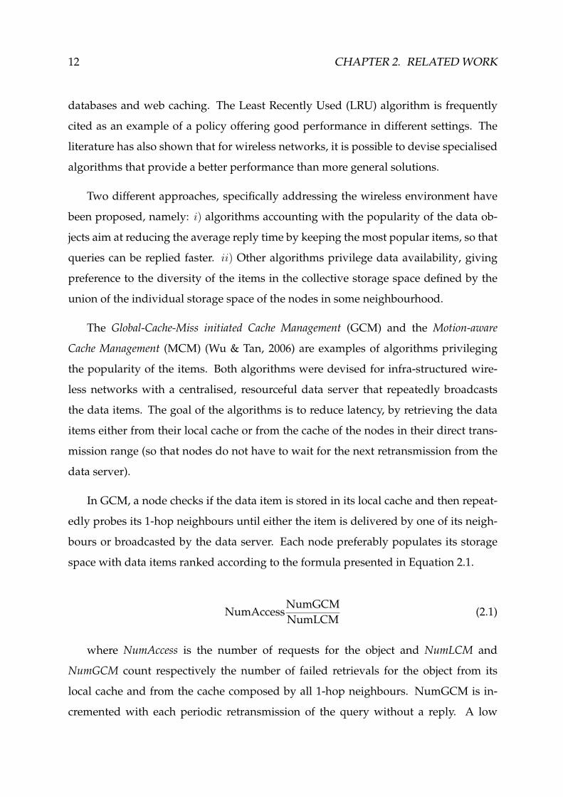
space with data items ranked according to the formula presented in Equation 2.1.
NumAccessNumGCM
NumLCM(2.1)
where NumAccess is the number of requests for the object and NumLCM and
NumGCM count respectively the number of failed retrievals for the object from its
local cache and from the cache composed by all 1-hop neighbours. NumGCM is in-
cremented with each periodic retransmission of the query without a reply. A low

2.2. LOCAL STORAGE MANAGEMENT 13
NumGCM represents either an item that is popular in the cache of the neighbours or
frequently broadcasted by the data server.
MCM ranks the candidates for replacement in local storage according to a “PIX” (P
InverseX) score, originally described in Acharya et al. (1995). PIX score is given by the
ratio of the access probability (P ) for the frequency with which the item is broadcast
by the data server (X). An interesting aspect of MCM is that the decision to cache an
item depends of the estimated availability of a replica stored on a node in proximity.
The future distance between two nodes is calculated by comparing their position, di-
rection and speed. Comparisons between GCM and MCM show that in general, GCM
outperforms MCM although at expenses of additional energy consumption.
In (Sailhan & Issarny, 2003), nodes in an hybrid network cache web pages, making
them available to other nodes. Each node ranks its cached web pages according to
their popularity and access cost. Popularity estimates the probability of future accesses
from past requests. The AccessCost estimates the cost of retrieving the web page from
another node, which may possible be located several hops away. Finally, the system
prefers to remove older and bigger documents.
Popularity is a relevant criteria when it is known that data will be available in
a bounded time. Other algorithms give priority to data availability, and therefore,
are more adequate for scenarios where such a bound does not exist. This is the most
expected scenario in MANETs. For example, in the algorithm described in (Lim et al.,
2006), a data item is only cached if the object was sent by a nodemore than a predefined
number of hops away. Cached data item are selected to be replaced by one of three Time
and Distance Sensitive (TDS) algorithms. TDS combines the distance to the closest node
known to also store a copy (δ) with the inverse of the time elapsed since the distance
was measured (τ ). τ is used to estimate the accuracy of the distance measurement. The
three TDS algorithms are:
TDS D given by δ + τ . Because δ ≥ 1 and 0 ≤ τ ≤ 1, it can be said that TDS D selects
the item with the lower δ and uses τ for tie-breaking;

14 CHAPTER 2. RELATEDWORK
TDS T that selects the item with the lowest τ .
TDS N which selects the lowest value of δ × τ .
Simulation results concluded that in general, the three algorithms perform better
than the traditional LRU (Least Recently Used) cache update policy. Of the different
TDS policies, no clear winer can be found, as they present different results depending
of the network settings. TDS algorithms have a limited application as they require
nodes to be equipped with location devices.
2.3 Data Dissemination Algorithms
Intuition suggests that there is a tradeoff between the effort placed on the dissem-
ination of the data and the effort required to retrieve it. In principle, a strategy that
saves the resources during the dissemination, for example by placing the replicas in
nodes close to the producer will require the consumption of more resources for data
retrieval. This observation motivated the classification adopted in this section, which
is depicted in Figure 2.2. At first, algorithms are arranged according to the level of
awareness of the nodes on the location of the data. The term location is used in a broad
sense encompassing both geographical location and node addresses. In this taxonomy,
a node is aware of the location of some data item if it knows either a geographical
coordinate or the address of a node and one of them can be used to retrieve the data
item.
Algorithms that are unaware of the location of data items are arranged by their ef-
fort on the geographical distribution of the replicas in two classes: “location unaware”
algorithms completely ignore the state of other nodes in the strategies for keeping data
items in their storage space; “Improved location unaware” algorithms perform some
form of leveraging of the replicas to prevent excessive redundancy in the neighbor-
hood of each node.

2.3. DATA DISSEMINATION ALGORITHMS 15
Data SourceKnown
LocationReplicaKnown Unknown Replica Topological
DistributionYes No
Unknown
QueryAddressedYes No
Trialand error
Server oriented Improvedlocation unaware
Locationaware unaware
Location
Figure 2.2: A taxonomy of data dissemination algorithms
On the opposite side of our classification are the algorithms that are aware of the
location of every replica. These algorithms have been grouped in a class named “lo-
cation aware”. The algorithms that are aware of only one copy are arranged by the
strategy used for performing the queries. The “server oriented” class groups the al-
gorithms that address the query to the location of the known copy of the data. As the
name implies, “trial and error” algorithms perform a preliminary step trying to find
some replica in a more favorable location than the one that is known.
2.3.1 Location Unaware Algorithms
Location unaware algorithms typically use the less efficient dissemination proce-
dures. Of the four algorithms described in this section, three perform on-demand repli-
cation, with nodes caching only the data that has been received in result of a query. An-
other common aspect of these algorithms is the absence of cooperative management of
the available distributed storage space.
A simple location unaware algorithm was used to estimate the equilibrium point
between the effort that should be placed on dissemination and retrieval (Krishna-
machari & Ahn, 2006). The goal is to determine the most adequate number of repli-
cas of a data item. In the algorithm, nodes disseminate data using point-to-point
messages addressed to random nodes. Queries progress in successive expanding-
ring search broadcasts with TTL increasing according to a dynamic programming se-

16 CHAPTER 2. RELATEDWORK
quence (Chang & Liu, 2004). The authors conclude that, in this setting, the optimal
number of replicas of each item is proportional to the square root of its query rate.
However, this result is of limited application because it assumes that the query ratio of
some item will be known by the producer. In addition, it should be expected that in
non-random deployment of the replicas, for example like those presented below, that
take into account the popularity of the data items, queries can use different sequences
of TTLs.
The Simple Search (SS) algorithm (Lim et al., 2006) was devised for hybrid networks.
It is assumed that nodes only keep items they have previously requested in their stor-
age space. Simple Search improves access latency for the cases where the requested data
is stored in some node closer than the data server, co-located with the base station.
In SS the queries are broadcasted to the network in a request message with a pre-
defined value in a Time-To-Live field. All nodes that receive the request packet and
do not store the object append their address to the request packet, decrement the TTL
field and, if the TTL field permits it, retransmit the packet. Instead of retransmitting
the request, nodes capable of replying to the request, including the data server, send
a point-to-point ack message to the source of the request. The ack message follows the
path accumulated in the request message. The querying node requests the object to
the source of the first ack message received using a confirm message and discards the
remaining. The data is delivered by the node that receives the confirmmessage.
In contrast with SS, the Rumour Routing, Static Access Frequency and Autonomous
Gossipping algorithms (described below) assume that nodes are simultaneously the
producers and consumers of data. Each assumes, however, a different networking
model. The Rumour Routing algorithm relies on the stability of the network links be-
tween the nodes and is therefore more adequate for sensor networks without node
movement. Autonomous Gossipping, instead, relies on the temporary links established
by moving nodes to disseminate data. Static Access Frequency considers that nodes are
in transmission range for some time interval.
Rumour Routing (Braginsky & Estrin, 2002) does not replicate data. Instead, it im-
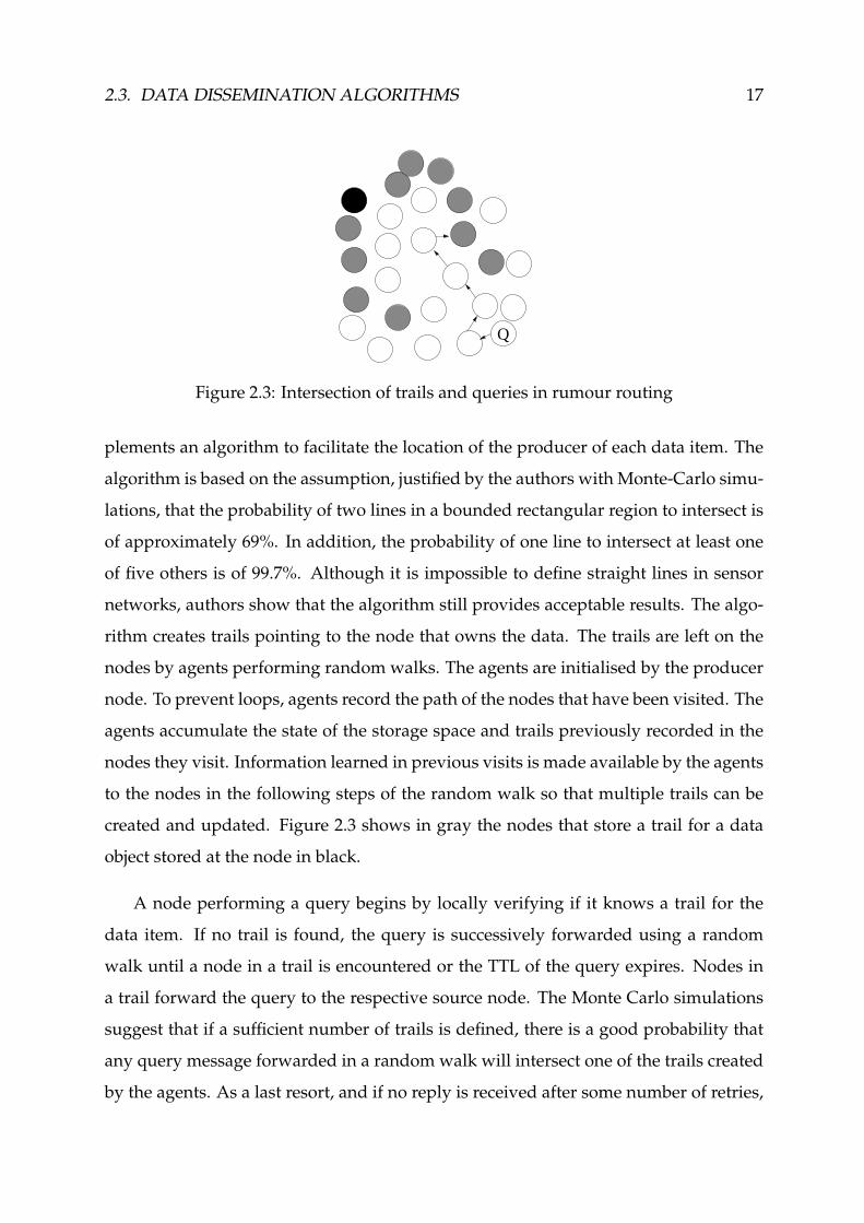
2.3. DATA DISSEMINATION ALGORITHMS 17
Q
Figure 2.3: Intersection of trails and queries in rumour routing
plements an algorithm to facilitate the location of the producer of each data item. The
algorithm is based on the assumption, justified by the authors with Monte-Carlo simu-
lations, that the probability of two lines in a bounded rectangular region to intersect is
of approximately 69%. In addition, the probability of one line to intersect at least one
of five others is of 99.7%. Although it is impossible to define straight lines in sensor
networks, authors show that the algorithm still provides acceptable results. The algo-
rithm creates trails pointing to the node that owns the data. The trails are left on the
nodes by agents performing random walks. The agents are initialised by the producer
node. To prevent loops, agents record the path of the nodes that have been visited. The
agents accumulate the state of the storage space and trails previously recorded in the
nodes they visit. Information learned in previous visits is made available by the agents
to the nodes in the following steps of the random walk so that multiple trails can be
created and updated. Figure 2.3 shows in gray the nodes that store a trail for a data
object stored at the node in black.
A node performing a query begins by locally verifying if it knows a trail for the
data item. If no trail is found, the query is successively forwarded using a random
walk until a node in a trail is encountered or the TTL of the query expires. Nodes in
a trail forward the query to the respective source node. The Monte Carlo simulations
suggest that if a sufficient number of trails is defined, there is a good probability that
any query message forwarded in a random walk will intersect one of the trails created
by the agents. As a last resort, and if no reply is received after some number of retries,

18 CHAPTER 2. RELATEDWORK
the algorithm broadcasts the query.
The Static Access Frequency (SAF) algorithm (Hara, 2001) tries to improve data avail-
ability in the presence of network partitions by predicting future access by the appli-
cations to the data items. SAF progresses in rounds. At the beginning of each round,
nodes rank the data objects by access frequencies and try to populate their storage
space with the data items with the highest ranks. Storage space must be occupied by
the designated objects. If some object cannot be retrieved, the storage space will re-
main free until the object is retrieved from the network. SAF is a simple algorithm that
does not require coordination between the nodes. This uncooperative behaviour will
likely replicate the most popular items a large number of times, decreasing the number
of items that could be retrieved from the neighbours.
SAF was extended to address the case where the access pattern of the nodes dis-
closes some correlation between different data objects (Hara et al., 2004) and to handle
periodic updates of data items (Hara, 2002). For clarity, the improved versions of the al-
gorithms (respectively C-SAF and E-SAF) are discussed together with other algorithms
proposed by the same authors in Section 2.3.2.
Autonomous Gossipping (Datta et al., 2004) uses ecological and economical prin-
ciples as an alternative to classical access frequency definitions. Autonomous Gossip-
ping considers each host to be an habitat providing storage space for a limited number
of data items. The habitat may be more or less favourable to the data item, depending
on the relevance of the data item to the host.
Both hosts and data items have a profile, defining respectively the topics of rele-
vance for the host and the topics covered by the data item. A function similarity numer-
ically rates the proximity of the profiles of hosts and data items. In addition, data items
carry an attribute describing the geographical locations where the item is supposed to
reside and a scalar called the associated utility, measuring the utility of the item to the
host. The utility of an item can be incremented for example when the item is used by
some application and decremented otherwise. Hosts advertise a goal zone to let data
items learn about their intended destination.

2.3. DATA DISSEMINATION ALGORITHMS 19
The system partially implements a “survival of the fittest” model. Opportunistic
gossipping, defined by the temporary interaction made available by the movement of
the nodes, is used for data items to evaluate the conditions of their hosts, and consider
their migration for more favourable habitats. Inside each host, data items compete for
their survival, knowing that the hosts attempt to maximise the accumulated associated
utility of the data items they host. When an opportunity appears, data items decide to
stay, migrate or replicate to another host with a more suitable profile, according to the
following policies:
Migration A data item decides to migrate when the host provides adverse conditions,
defined by a similarity below some threshold and low utility. The decision to
migrate is taken without the data items becoming aware if the migration will
provide better conditions.
Replication A data item may decide to replicate if it has an high utility and similarity
above a threshold. To prevent an excessive population of some data item, and
again following the ecological model, the utility of the original data item and its
replica will be lower than its value before replication.
Replica reconciliation occurs when a data item finds a copy of itself in the host to
where it has migrated. The utility of the re-conciliated data item is higher than
the utility of both replicas.
Migration anyway Independently of the friendliness of its current habitat, a data item
may decide to migrate if the current host is outside its target location (if any).
Migration is attempted to hosts whose goal zone is the same of the data item.
Simulation results (Datta et al., 2004) confirmed that autonomous gossipping is ca-
pable of delivering messages to a large proportion of the interested nodes. However,
it leaves some questions unanswered. Intuition suggests that an high threshold may
result in nodes becoming excessively judicious about the hosted data items what may
endanger the message dissemination. This can be compensated either by increasing

20 CHAPTER 2. RELATEDWORK
the size of the habitat or the frequency of contacts so that the probability of finding an
interested node is increased. However, simulation results presented are not sufficient
to evaluate this tradeoff.
2.3.2 Improved Location Unaware Algorithms
Although unaware of their precise location, improved location unaware algorithms
use some form of topological information to distribute the replicas. This section
presents three examples. The first degrades the accuracy of the information with the
distance to the source. In the remaining, nodes in proximity cooperate to improve data
availability by coordinating the content of their storage space.
The concept of non-uniform information is introduced in Tilak et al. (2003) to describe
one application model for sensor networks where the relevance of the information de-
grades with the distance from the source to the consumer. In the non-uniform informa-
tion model it is assumed that instead of delivering data to powerful sink nodes, fixed
over the network, sensor nodes will deliver data to “passing by” sink nodes. Examples
are military applications, where the presence of enemies nearby is more relevant than
learning about a distant fight.
Two categories of algorithms are presented in the paper to limit the propagation of
the information: deterministic and randomised. In both, the goal is to progressively
reduce the number of forwarders of every message by successively applying at each
hop a mechanism that only propagates some of the messages it receives. In the Fil-
tercast deterministic algorithm, each node forwards every nth message received from
the same source. However, if all nodes are configured with the same constant, all will
propagate the same message from each source. If this synchronisation is removed, the
accuracy of the information propagated is improved. This is addressed in the RFilter-
cast deterministic algorithm, where although forwarding every nthmessage, each node
initially peaks a random number that will decide which of the nmessages is transmit-
ted. Simulation results showed that using RFiltercast, nodes transmit more messages

2.3. DATA DISSEMINATION ALGORITHMS 21
than with Filtercast. Both deterministic algorithms present some scalability problems
as they require that each node keep a counter for each source.
Randomised algorithms are stateless and therefore scale better with the size of the
network. In the unbiased algorithm, each packet is retransmitted with an independent
probability. The biased algorithm, in turn, improves the probability of retransmission
for packets with an higher Time-To-Live field, what corresponds to an higher proximity
to the source.
Non-uniform information algorithms effectively reduce the number of retransmit-
ted messages and therefore, contribute to increase the network lifetime by saving
node’s batteries. However, the lack of semantic interpretation of the filtered data raises
concerns of the utility of these algorithms.
The Dynamic Access Frequency and Neighbourhood (DAFN) and the Dynamic Con-
nectivity based Grouping (DCG) algorithms (Hara, 2001) predict the items that will be
accessed by each node in the future from previous accesses. Like in SAF (described in
Section 2.3.1), the estimation is used to improve data availability in the presence of net-
work partitions. Both algorithms progress in rounds. At each round, nodes re-evaluate
their access pattern to the data and negotiate with their neighbours the data items that
should be stored so that data availability is improved for the group.
In DAFN, nodes negotiate with their 1-hop neighbours. Each round begins with
the broadcast of a message by every node. The message notifies the neighbours about
the presence of the node and includes information about the node’s access frequency to
the data items. Nodes then follow a deterministic algorithm to populate their storage
space. For each 1-hop neighbouring set of nodes, the algorithm is sequentially applied
from the one with the lowest ID to the one with the highest. If two neighbouring nodes
intend to store the same data item, the algorithm dictates that:
• If one of the nodes is the producer of the object, the other node will not store it;
• If none of the nodes is the producer of the object, the item is stored by the node
with the highest access frequency.

22 CHAPTER 2. RELATEDWORK
The storage space made available by duplicate elimination will be filled by the next
objects in the node’s rank. If some node cannot retrieve an object from the network, the
space will be temporarily filled with some other object until the node is able to retrieve
a replica of the preferred object.
Although DAFN improves replica distribution over SAF, it still allows some re-
dundancy between nodes two or more hops away. However, it should be noted that
the major goal of replication is to improve availability. Therefore, some tradeoff must
be found between the number of replicas of each data item that can be reached by
the nodes and the probability of, in the future, none of the nodes storing them to be
reachable. DCG estimates this probability by counting the number of links that must
be broken between any two nodes. Instead of using 1-hop neighbours, DCG groups
nodes connected by at least two disjoint paths and removes replica redundancy among
them. Each group estimates their access frequency to the data items by summing the
access frequency of all its members. Data items are allocated to the node with the
highest access frequency for the item.
DCG is the most effective of SAF, DAFN and DCG algorithms in the removal of
redundancy. However, it is also the one requiring the more power consuming oper-
ations. In dense networks, i.e. those where a large number of nodes can be reached,
DCGwill require the transmission and forwarding of a large number of messages. An-
other benefit of replication, not considered in DCG, is the improvement of the access
latency to the data. DCG may increase latency in large scale networks because it will
likely increase the average distance of each node to the replicas of the items.
Simulations assumed a random movement of the nodes and experimented differ-
ent access patterns to the data. DCG showed to be the best performing one for every
scenario at the expenses of the highest number of messages. The most interesting re-
sults are presented with increasing levels of randomness in the queries. The more
random the queries, the more the performance of the three algorithms approximates.
However, DCG continuously increases traffic while the traffic in DAFN tends to be
reduced and in SAF it is constant and significantly lower. Finally, simulations con-

2.3. DATA DISSEMINATION ALGORITHMS 23
firm that the performance of all the algorithms is highly by the number of neighbours
and the storage space at each node. In extreme cases, any of the algorithms performs
equally. The availability of the data can be differentiated only for the intermediary
cases. However, the same conclusions do not apply to the traffic, being even impossi-
ble to establish a correlation between the traffic and the data availability results.
SAF, DAFN and DCGwere extended respectively to C(Correlation)-SAF, C-DAFN
and C-DCG to address the case where the access patterns discloses some correlation
between independent data items (Hara et al., 2004). The strength of correlation is de-
fined for each node and pair of items as the frequency of access to the two items by
the node. It is assumed that the strength of correlation between each two data items
is known and does not change. In these algorithms, the access frequency is replaced
by the data priority, estimated by each node from the access frequency of the item and
from the sum of the strength of the correlations of the item with all other items.
Evaluation was performed by comparing the original methods with those using
correlation in a network where nodes request data items with a correlation predefined
by the authors. The performance of each algorithm relative to each other mimics the
results presented in the original version. In this scenario, correlation-aware methods
provide better accessibility than non-correlation methods while increasing the traffic
at the nodes.
E(xtended)-SAF, E-DAFN and E-DCG handle periodic updates of the data ob-
jects (Hara, 2002). The algorithms assume that items are periodically updated with
a known and constant rate. The access frequency metric for each item is replaced by a
PT value representing the average number of access requests which are issued for an
item until its next update. PT is given by pij.τj , where pij is the access frequency of
nodeNi to itemDj and τj denotes the time remaining until the next update of itemDj .
Preference is given to replicate data objects with higher PT values as they represent the
objects that will be valid for more time and with an higher access ratio.
Simulation results show that when the frequency of the updates is significantly
higher than the frequency of the rounds, the rapid invalidation of the caches attenuates

24 CHAPTER 2. RELATEDWORK
the gains of the extended algorithms. However, the frequency of the rounds can not be
excessive because previous results (Hara, 2001) showed that it significantly increases
traffic.
2.3.3 Trial and Error Algorithms
In the “trial and error” and “owner oriented” classes of algorithms, nodes are
aware of the ID or location of the primary copy of the data but not of the replicas.
These classes are distinguished by the effort put by the querying node in retrieving the
data from the replicas. In general, trial and error algorithms weight the cost of address-
ing the query to the server or perform a preliminary round probing a limited number
of nodes for the data and select the most advantageous option. In some algorithms,
and in the absence of failures, the preliminary round always succeeds and is the de-
fault mode of operation. The examples below show the application of trial and error
algorithms in two distinct types of networks: hybrid networks and sensor networks
where nodes are equipped with location devices.
A simple example of a trial and error algorithm for hybrid networks is 7DS (Pa-
padopouli & Schulzrinne, 2001). In 7DS, each node can be in one of two modes: infra-
structured or ad hoc. If the node is in range of a base station, queries are directly ad-
dressed to it. Otherwise, queries are broadcasted to the node’s 1-hop neighbours and
replied by those having the resource in their local cache. Resources are only cached by
nodes that have previously requested them.
The 1-hop query propagation of 7DS limits the probability of successful retrieval of
the data. The algorithm described in (Sailhan & Issarny, 2003) removes this limitation.
It aims specifically at caching web information in hybrid networks but could be easily
extended for other application domains. In this algorithm, nodes create profiles of
other nodes. A profile describes the interests of a node and are created by observing
the queries the node sends.
The algorithm is tightly integrated with the Zone Routing Protocol (ZRP) (Haas,

2.3. DATA DISSEMINATION ALGORITHMS 25
1997). The ZRP combines reactive and proactive mechanisms. Each node pro-actively
collects routing information for the nodes in its neighbourhood (the “zone” of the
node). Routing information for nodes outside its zone is collected on-demand.
The algorithm operates in two phases: replica location and data retrieval. Replicas
are located by successively performing a sequence of steps from the one with the low-
est cost for retrieving the data to the one with the highest cost. The steps performed
are:
1. If an access point is located in its zone, the data is retrieved from the access point;
2. The node broadcasts a query to the nodes in its zone;
3. The node sends point-to-point queries to some nodes outside the zone but at
a lower distance than the data server. The nodes selected are those known to
have a profile matching the requested web page, ordered according to a rank
that weights the node’s profile and the distance, in hops, between them.
4. The query is sent to the closest access point.
Only positive replies are sent to the querying node. If several replies are received,
what may happen in Steps 2 and 3, nodes are ranked by weighting the distance (in
hops), the freshness of the data and the resources available on the node for each reply.
The resource is requested to the most suitable node.
Double rulings algorithms are an example of trial and error algorithms for sensor
networks where the devices are aware of their location. These algorithms use sphere
projections to determine the location of the replicas so that they form a circle as de-
picted in Figure 2.4. The work described in (Sarkar et al., 2006) uses stereographic
projections.
In this algorithm, the area of the sensor network is considered as a finite region of
the plane. Since the stereographic projection maps a plane in a sphere, the sensor net-
work is mapped in a region of the sphere. The rationale for this algorithm comes from

26 CHAPTER 2. RELATEDWORK
Q
Figure 2.4: Storage and query circles in Double Ruling storage
noticing that in a sphere, any two great circles intersect. Double rulings algorithms
use one such great circle for determining the location of the replicas and another for
forwarding the queries.
In double ruling all nodes can derive the location of the primary copy from a map-
ping of the key or type of the data in a geographical coordinate inside the network
perimeter. This mapping is usually referred as Geographical Hash Tables (GHTs) due
to its similarities with Distributed Hash Tables (DHTs), which map the key of a data
item on an address.
Every data object is stored along the projection on the plane of the great circle pass-
ing by the producer and the hash of the data type given by a GHT. Storage is performed
by nodes forwarding the object along the circle. A property of the storage circle is that,
independently of the location of the source, it necessarily includes the hash point and
its antipode point in the sphere. The nodes closer to these locations perform aggre-
gation functions that speed up and reduce the amount of energy required to retrieve
data summaries. Figure 2.4 shows two storage circles and represents in black these two
points.
Data summaries can be retrieved by addressing the queries using any geographical
routing algorithm (like GPSR (Karp & Kung, 2000) or other) to the hash point or to its
antipode. Data can be retrieved by having the query to follow any closed curve that
separates the two hash points, knowing that the curve finds a replica of every data

2.3. DATA DISSEMINATION ALGORITHMS 27
object stored.
The trial and error classification of this algorithm comes from noticing that any
data item will eventually be found if the query is forwarded along a query curve. A
query curve is depicted in a dashed circle in Figure 2.4. The curve is determined by
an algorithm that first rotates the sphere so that the hash point is placed at the top of
the sphere and then deriving a latitude circle over the sphere. It is shown in the paper
that, if the distance between the producer of the item and the querying node is d, the
distance to the closest replica is in the order ofO(d). Double ruling algorithms have the
desirable property of avoiding traffic concentration at the hash points, thus improving
fairness and load balancing.
The Geographical Location Service (GLS) (Li et al., 2000) was designed to facilitate
the mapping of node identities on their current location but can be applied in other
domains. All nodes have an unique identity, selected from a circular identity space.
The goal of the algorithm is to facilitate the retrieval of the approximate location of
any node from its identity, so that a geographical routing algorithm like GPSR (Karp &
Kung, 2000) can be used for packet forwarding.
The algorithm assumes that all nodes are aware of a geographical partition of the
networked region. A simple example is to partition the network in squares, as depicted
in Figure 2.5. An hierarchy is established with squares of order n being successively
grouped in squares of order n+1with sides that double the size of the squares of order
n. A fundamental requirement of the algorithm is that each square of order n is part of
precisely one square of order n + 1. Figure 2.5 shows 16 order 1 squares, grouped in 4
order 2 squares and in one order 3 square.
The algorithm geographically distributes the information by the network. Some
node S, updating its location, registers the information with progressively lower den-
sity of replicas as the size of the squares increases. The location of S will be stored at
each square of order 1 in the square of order 2 where S is located. One copy will be
stored at each of the remaining squares of order 2 that share the same order 3 square,
etc. In practice, S stores 3 replicas at each level of the hierarchy. Figure 2.5 depicts

28 CHAPTER 2. RELATEDWORK
Figure 2.5: Network region partitioning in GLS
in gray a possible deployment of the replicas. Replicas of the location of S are stored
at the node with the least identity greater than the identity of S on the target region.
However, the effective identity of the nodes storing the replica is unknown to S. In-
stead, the packet is forwarded to some point in the target square using geographical
routing. The first node in the respective square that receives the packet will use the
same algorithm followed by queries (described below) to find the target node.
A node issuing a query for S and not locally storing S’s location will forward it to
the node with the closest identity of which it stores the location. Nodes successively
perform a similar operation until a reply to the query is found. It should be noted that
this algorithm converges by approximating the query to some node storing the replica.
It was shown that the number of forwardings is not more than the order of the square
on which the querying node and S are co-located (Li et al., 2000).
2.3.4 Owner Oriented Algorithms
In owner oriented algorithms, queries are addressed to the node known to hold the
item. This section presents two variations of owner oriented algorithms. One imple-
ments a transparent caching mechanism in hybrid networks. In the second, queries are
always replied by the owner node. Replicas are made available to tolerate faults and
node movement.
In the Cache the Data (CacheData) protocol (Yin & Cao, 2006) requests are always
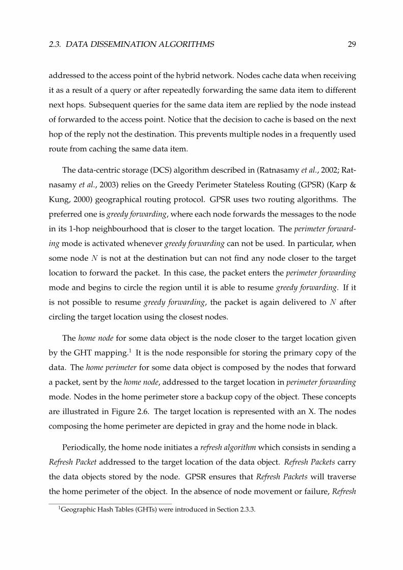
2.3. DATA DISSEMINATION ALGORITHMS 29
addressed to the access point of the hybrid network. Nodes cache data when receiving
it as a result of a query or after repeatedly forwarding the same data item to different
next hops. Subsequent queries for the same data item are replied by the node instead
of forwarded to the access point. Notice that the decision to cache is based on the next
hop of the reply not the destination. This prevents multiple nodes in a frequently used
route from caching the same data item.
The data-centric storage (DCS) algorithm described in (Ratnasamy et al., 2002; Rat-
nasamy et al., 2003) relies on the Greedy Perimeter Stateless Routing (GPSR) (Karp &
Kung, 2000) geographical routing protocol. GPSR uses two routing algorithms. The
preferred one is greedy forwarding, where each node forwards the messages to the node
in its 1-hop neighbourhood that is closer to the target location. The perimeter forward-
ingmode is activated whenever greedy forwarding can not be used. In particular, when
some node N is not at the destination but can not find any node closer to the target
location to forward the packet. In this case, the packet enters the perimeter forwarding
mode and begins to circle the region until it is able to resume greedy forwarding. If it
is not possible to resume greedy forwarding, the packet is again delivered to N after
circling the target location using the closest nodes.
The home node for some data object is the node closer to the target location given
by the GHT mapping.1 It is the node responsible for storing the primary copy of the
data. The home perimeter for some data object is composed by the nodes that forward
a packet, sent by the home node, addressed to the target location in perimeter forwarding
mode. Nodes in the home perimeter store a backup copy of the object. These concepts
are illustrated in Figure 2.6. The target location is represented with an X. The nodes
composing the home perimeter are depicted in gray and the home node in black.
Periodically, the home node initiates a refresh algorithm which consists in sending a
Refresh Packet addressed to the target location of the data object. Refresh Packets carry
the data objects stored by the node. GPSR ensures that Refresh Packets will traverse
the home perimeter of the object. In the absence of node movement or failure, Refresh
1Geographic Hash Tables (GHTs) were introduced in Section 2.3.3.

30 CHAPTER 2. RELATEDWORK
X
Figure 2.6: Home node and perimeter in Data-Centric Storage
Packets are equally used to signal the availability of the home node.
Nodes receiving a Refresh Packet enter or update the data object in their caches.
Therefore, nodes that recently joined the home perimeter are implicitly included in the
list of replicas. Additionally, each node in the home perimeter compares its distance
to the target location with the distance of the home node to the target location. If
closer, the node elects himself as the new home node. Others (including the previous
home node) will be notified by an updated Refresh Packet. It should be noted that this
procedure implicitly addresses the case where the home node moves away from the
home perimeter.
Nodes in the home perimeter may also initiate the refresh algorithm if they do not
receive a refresh packet after a predefined amount of time. This procedure triggers the
replacement of a failed home node and will trigger the election of a new one.
An interesting case occurs when a home node issues a refresh packet for a data object
but never receives it. This implicitly indicates to the node that it is no longer included
in the home perimeter what may occur either because the node moved away or because
some other node became closer to the target location. After a predefined timeout with-
out receiving any refresh packet, nodes purge the data object from their caches.

2.3. DATA DISSEMINATION ALGORITHMS 31
2.3.5 Location Aware Algorithms
In location-aware algorithms, nodes know the location of both the primary copy of
the data and its replicas. This section presents three examples of these algorithms. The
first two are designed for hybrid networks. The third extends DCS by geographically
distributing the replicas and uses a deterministic algorithm to derive their location.
The Cache the Data Path (CachePath) (Yin & Cao, 2006) algorithm was designed
for hybrid networks. Nodes store the replies to their queries. Intermediary hops that
forward the reply record the key of the item and the destination of the message.
Queries are always addressed to the access point. However, a node forwarding a
query may redirect it, if it is aware of a replica of the item in a node located closer than
the access point. Nodes rely on the underlying routing protocol to learn the distance (in
hops) to the access point and to the caching node as well as to forward the messages.
In comparisonwith CacheData (presented in Section 2.3.4), CachePath requires less
storage space because only an address, not the object is stored. In addition, the algo-
rithm implements some mechanisms to prevent nodes from storing useless informa-
tion. Nodes that are closer to the access point than to the destination of a reply do not
record information because it is more cost efficient to forward the query to the access
point. Also, because node movement can rapidly invalidate distance information, ad-
dresses are cached only if the replica is stored up to a maximum predefined distance.
Nodes that redirect queries are responsible for confirming the availability of the data
item or to retransmit the query to the access point if the object is not provided.
Analytical comparisons showed that CachePath and CacheData present advan-
tages over a baselinemethodwhere all queries are forwarded to the data centre. Cache-
Data outperforms CachePath when the storage space available at the nodes is larger,
when data items are frequently updated or the topology changes. In the opposite
situations, CachePath is preferable. HybridCache (Yin & Cao, 2006) selects the most
favourable of CachePath and CacheData on a per-query basis according to three rules:

32 CHAPTER 2. RELATEDWORK
X
XX
X
Z1 Z2
Z4 Z3
Figure 2.7: Monitor nodes in Resilient-Data-Centric Storage
• CacheData is used if the data item is small;
• CacheData is used if the object is frequently updated. CachePath is used other-
wise;
• CachePath is used when the gains (in hops) are significant, i.e. when the distance
to the data centre is high in comparison with the distance to the caching node.
Simulation results showed that HybridCache outperforms CacheData and CacheP-
ath.
Storing the replicas of each data item in proximity is considered undesirable be-
cause such a system is unable to tolerate localised failures which may result for
example from interference (Ghose et al., 2003). Resilient Data-Centric Storage (R-
DCS) (Ghose et al., 2003) improves data availability by geographically partitioning the
network in zones and storing at most one replica on each zone (see Figure 2.7). R-DCS
implements a two layer architecture, with some nodes storing replicas of the data and
others keeping summaries of the cached information. R-DCS extends the GHT func-
tion with a zone parameter so that a different location, within the zone, is returned
for each zone. Like in DCS (described in Section 2.3.4), the node closer to the target
location in each zone is the home node for the object. In R-DCS, this node is named the
“monitor node”.
Data storage is optional for monitor nodes and depends of its available resources.
Amonitor node that simultaneously stores data is called a replica node. At aminimum,
2.3. DATA DISSEMINATION ALGORITHMS 33
any monitor node is required to store a map containing:
• A list of the zones containing replica nodes;
• A list of the zones containing monitor nodes;
• Event summaries, to facilitate summary-mode queries;
Data objects are stored by forwarding them to the corresponding monitor node in
the source’s zone. If the monitor node is not storing data, it will forward the object
to the closest replica node. All queries are also addressed to the monitor node in the
region of the source. Depending on the type of the query, the monitor node will either
reply directly (if it is a summary query) or forward the request to all other monitor
nodes so that each can reply with the information stored locally.
Monitor nodes coordinate to keep updated versions of the map using a virtual ring
(depicted in Figure 2.7). Each monitor node receiving the map updates it with the
information it collected since the last visit and forwards the map to the next node in
the ring.
2.3.6 Discussion
This section surveyed different algorithms for data dissemination in wireless net-
works. As depicted in Table 2.1, the algorithms cover a large number of combinations
of assumptions concerning the capabilities of the devices, their movement, the sup-
porting infrastructure and the predictability of the accesses to each data item.
The table shows some correlations among different algorithms. For example, the
absence of proactive dissemination of replicas can be found in all algorithms devel-
oped for hybrid networks (those with a small number of producers) but also in others
developed for wireless networks without infrastructure support. With the exception of
Rumour Routing, all these algorithms create copies of the data items by storing them
on the nodes performing the queries. Replication is justified, for example, to improve

34CHAPTER2.RELATEDWORK
Class ProtocolNode
Movement
Location
Awareness
Access
PredictionProducers
Replica
Refresh/
Leveraging
Geograph.
Distr.
Message type
Proactive
Dissem.Query
Location
Unaware Simple Search • << n – B
Rumour Routing n rw rw
*-SAF • • n ◦ –
Aut. Gossipping • • n ◦ opp –
Improved Non-Unif n local/degrad. B –
*-DAFN • • n ◦ coordination –
*-DCG • • n ◦ coordination –
Trial&
Error
7DS • << n – p2p/B
Sailhan et al. • << n – p2p
Double rulings • n deterministic p2p p2p
GLS • • n ◦ deterministic p2p p2p
Owner CacheData • << n local – p2p
DCS • • n • p2p p2p
Loc.
Aware
CachePath • n – p2p
R-DCS • • n • deterministic p2p p2p
•: feature of the algorithm ◦: implicitly provided
n: approx. all nodes in the network, << n: small number of nodes
rw: random-walk, B: broadcast, p2p: point-to-point message, opp: opportunistic, –: not applicable
Table 2.1: Comparison of the data dissemination algorithms surveyed

2.3. DATA DISSEMINATION ALGORITHMS 35
availability (Hara, 2001) and to reduce of the number of transmissions (Sailhan & Is-
sarny, 2003).
Replica refreshment can be used to ensure that an adequate number of replicas exist
or that they are at the correct location. Some protocols offer this feature as a side effect
of the protocol’s normal operation. DCS and R-DCS are the only two protocols that
implement specific measures to ensure that replicas are kept at the correct location.
They send periodic messages, which are also used as keep alive messages, and that
trigger a reconfiguration in case of failure.
The geographic distribution of the replicas should be interpreted differently for
algorithms with and without proactive replica dissemination. Proactive algorithms
distribute the replicas by the networked region. Non-proactive algorithms are mostly
motivated by the savings in the resources of the nodes and aim to prevent that many
replicas are stored in a neighborhood. The non-uniform information algorithm (Tilak
et al., 2003) uses a particular case of geographic dissemination because it is the only
one that degrades the quality of the information with the distance to the source.
In the algorithms surveyed, proactive and geographic distribution of replicas is
an exclusive of the algorithms that benefit of location information. Geographical dis-
tribution is motivated, for example, by the improved resilience to localised failures,
like interference (Ghose et al., 2003). The three algorithms providing this feature ap-
ply deterministic functions (GHTs) to determine the location of the data. Deterministic
functions provide two advantages: i) they avoid expensive coordination operations
among the nodes to prevent redundancy, and ii) they allow all operations to be im-
plemented with point-to-point messages, which are expectedly less energy consuming
than broadcasts. A requirement typically neglected in the literature and affecting these
algorithms is that, to be useful, GHTs must first learn the topology of the entire net-
work so that all data keys can be mapped on coordinates inside the network.
Two methods are used for distributing replicas in non proactive replication algo-
rithms. In CacheData (Yin & Cao, 2006), the node selected for storing a replica is the
node located at the injunction of different routes to the access point. This implicitly

36 CHAPTER 2. RELATEDWORK
prevents multiple nodes in a single but frequently used route from redundantly stor-
ing the same data item. Nodes in DAFN and DCG (Hara, 2001) periodically initiate
rounds aimed specifically at negotiating the content of the cache of each node.
Point-to-point messages are the preferred method for message dissemination in al-
gorithms where the location of at least one copy is known. It should be noted that
point-to-point messages hide an implicit cost: these messages are typically delivered
to some underlying routing protocol which is responsible for finding the route to the
destination, or, in some cases, the most adequate next hop. To perform these oper-
ations, many routing protocols developed for networks where nodes are unaware of
their location, like DSR (Johnson et al., 2001) and AODV (Perkins & Royer, 1999) may
occasionally use broadcasts.
Location unaware algorithms cannot address point-to-point messages to a specific
node. However, even in this case, broadcast is used by a limited number of algorithms.
Alternatives are to rely on sequences of random point-to-point messages within neigh-
bours (randomwalks) or communicate onlywhen new nodes become in range (Oppor-
tunistic Gossipping). Node discovery is typically performed using limited broadcasts.
2.4 Packet Dissemination
The goal of the packet disseminationmodule is to propagate messages according to
the requirements of the query and dissemination algorithms. As shown in the previous
section (see Table 2.1), the preferred packet dissemination algorithm is point-to-point
what is typically provided by some routing protocol. Point-to-point routing protocols
for multi-hop wireless networks have received considerable attention in the literature.
The interested reader is referred to (Liu & Kaiser, 2003) for an extensive survey on the
subject.
Random-walks, opportunistic communication and broadcast have also been re-
ferred in the previous section as alternative mechanisms used for message propaga-

2.4. PACKET DISSEMINATION 37
tion. However, random walks and opportunistic communication are too restrictive
and show to be useful only in a limited number of scenarios. Both are probabilistic,
best effort mechanisms, that can not assure a timely message delivery or a successful
delivery of the messages even if it is possible to establish a communication channel
between two endpoints.
Broadcast does not suffer from the problems mentioned above but it is typically
avoided due to its considerable costs when compared with point-to-point messages.
However, due to the decentralised nature of Mobile Ad hoc NETworks (MANETs),
many services, like the location of some resource, are typically implemented using
broadcasts. Besides the data distribution protocols mentioned in the previous sec-
tion, examples of other applications implemented using broadcasts are route discov-
ery (Johnson et al., 2001; Perkins & Royer, 1999), reputation systems (Perich et al., 2004)
and the distribution of code updates for sensors (Levis et al., 2004).
This section focus on algorithms aimed to reduce the cost of broadcast operations.
We note that reducing the cost of broadcast operations indirectly helps to improve the
performance of the data distribution protocols that use point-to-point message deliv-
ery as many routing protocols use broadcast for determining the route for a node.
2.4.1 Broadcast Algorithms
The number of nodes required to retransmit a message so that it gets delivered
to every participant depends of several factors like the transmission range of the de-
vices, the location of the source, the size of the region covered by the nodes or their
geographical distribution. Furthermore, these factors may be permanently changing,
even between consecutive messages. In some cases, the underlying infrastructure may
provide the tools to efficiently broadcast messages. This is the case, for example, of
spanning trees provided by multi-cast routing protocols for ad hoc networks. How-
ever, in many cases, maintaining such structure is too costly or even impossible due
to the high mobility of the nodes. This section will focus on alternatives that do not

38 CHAPTER 2. RELATEDWORK
1: msgSet← {}
2: upon event RECEIVE(m) do3: ifm 6∈ msgSet then4: DELIVER(m)5: msgSet← msgSet
⋃
{m}6: SEND(m)7: end if8: end upon
Figure 2.8: Flooding algorithm
require an underlying infrastructure.
The most common implementation of broadcast is by flooding the network. In
flooding, each node keeps a log of the messages recently received. When a node re-
ceives a message for the first time, the node adds the unique identification of the
message to its log and retransmits it. Figure 2.8 shows an algorithm implementing
flooding. Flooding creates a large number of redundant transmissions. Many nodes
receive multiple copies of the message, each transmitted by a different node. There-
fore, it wastes a non-negligible amount of bandwidth and power. Independently of
the contribution of each retransmission, it consumes resources at the sender. Further-
more, receivers also spend a non-negligible amount of energy at the reception (Feeney
& Nilsson, 2001) and CPU time to decide if the message should be discarded or re-
transmitted. Finally, flooding may generate collisions and contention because most of
the Medium Access Control (MAC) protocols for ad hoc networks, like the one used
in the IEEE 802.11 (IEEE 802.11, 1999), lack a coordination function able to completely
avoid collisions of concurrent transmissions.
In a flooding procedure, the redundant reception of messages can not be com-
pletely avoided. Elsewhere (Tseng et al., 2002), it was shown that a retransmission
necessarily overlaps at least 39% of the region already covered by a previous transmis-
sion. Themotivation for devising algorithms that improve the performance of flooding
comes from noticing that this value increases significantly with the number of retrans-
missions listened by a node. The same paper shows that after listening to four trans-

2.4. PACKET DISSEMINATION 39
Uses:p: probability of retransmission
1: msgSet← {}
2: upon event RECEIVE(m) do3: ifm 6∈ msgSet then4: DELIVER(m)5: msgSet← msgSet
⋃
{m}6: if RANDOM(0,1)< p then7: SEND(m)8: end if9: end if10: end upon
Figure 2.9: GOSSIP1(p) algorithm
missions of the samemessage, a retransmission will overlap on averagemore than 95%
the region covered by the previous ones.
2.4.2 Probabilistic Algorithms
A simple approach to reduce the number of retransmissions of a broadcast is to
have each node to forward the first received copy of every message according to some
probability. This section describes a family of probabilistic algorithms named GOSSIP,
all presented in (Haas et al., 2002).
The simpler implementation of a probabilistic algorithm is GOSSIP1(p), where each
node, after receiving amessage for the first time retransmit it with some probability p ≤
1. GOSSIP1(p) is depicted in Figure 2.9. It should be noted that for p = 1, GOSSIP1(p)
becomes the flooding algorithm described previously.
GOSSIP1(p) presents some limitations that are better explained in a simplified
model assuming that the algorithm progresses in rounds. In this model, the source
of the message initiates the broadcast in round r = 0. A node receiving a message
for the first time in round r will possibly transmit it in round r + 1. Nodes receive a
transmission in the same round where it was transmitted.

40 CHAPTER 2. RELATEDWORK
An interesting property of probabilistic algorithms is that for the majority of the
broadcasts, either a large or a small proportion of the nodes receive the broadcast. This
property is usually referred as a bimodal behaviour and was studied in the context
of probabilistic algorithms for broadcasting in wireless networks in (Haas et al., 2002).
Let tr be the number of nodes that retransmit a message in round r and nr the number
of nodes that received it for the first time in the same round. In GOSSIP1(p), tr+1 is
expected to be close to nr× p < nr. Given that p is a constant, the probability of having
some nodes to retransmit the message in round r + 1, i.e. tr+1 > 0 increases with nr
which in turn depends of tr. Therefore, the broadcast is more likely to be delivered to
every node if, in all rounds, tr is high. The bimodal behaviour of GOSSIP1(p) comes
from the broadcast being initiated by a single node, so t0 = 1. If the number of neigh-
bouring nodes (nr) or the probability of retransmission (p) is also small, there is the risk
that after a few rounds, the broadcast dies because nr × p ≈ 0. However, with some
probability, it is also possible that nr increases rapidly in the first few rounds, ensuring
the delivery of the message to a large proportion of the nodes.
To avoid the bimodal behaviour one should therefore improve the operation of the
first few rounds. Because the number of neighbours (nr) does not depend of the algo-
rithm, an higher tr can only be achieved with an higher probability of retransmission p.
GOSSIP1(p, k) extends GOSSIP1(p) by setting p = 1 in the first k rounds of a broadcast.
In the remaining rounds, nodes retransmit with probability p < 1. The algorithm is
depicted in Figure 2.10.
Experimental results confirmed that for p > 0.7 and k = 4, GOSSIP1(p, k) does
not exhibit bimodal behaviour, meaning that only approximately 70% of the nodes
are required to propagate a broadcast to deliver it to a large proportion of the nodes
with high probability. For lower values of p, the delivery ratio of GOSSIP1(p, k) decays
rapidly. The problem was attributed to the irregular distribution of the nodes. In
regions with low density, the conditions that motivated GOSSIP1(p, k) may appear as a
result of a small number of nodes listening to the message for the first time, even after
a large number of rounds.

2.4. PACKET DISSEMINATION 41
Uses:p: probability of retransmissionk: min number of hops
1: msgSet← {}
2: upon event RECEIVE({m,hops}) do3: ifm 6∈ msgSet then4: DELIVER(m)5: msgSet← msgSet
⋃
{m}6: if hops < k ∨ RANDOM(0,1) < p then7: SEND({m,hops+1})8: end if9: end if10: end upon
Figure 2.10: GOSSIP1(p, k) algorithm
The problem can be addressed by monitoring the network so that an higher
probability of retransmission is applied in regions where the node density is low.
GOSSIP2(p1, k, p2, n) is depicted in Figure 2.11. In this algorithm, p1 and k retain the
meaning described for GOSSIP1(p, k). p2 > p1 specifies the probability of retransmis-
sion for nodes receiving the message from a node with less than n neighbours. Sim-
ulations showed that for the same scenarios, GOSSIP1(0.8,4) presented a comparable
performance to GOSSIP2(0.6,4,1,6). However, GOSSIP2 required on average less 13%
transmissions than GOSSIP1.
An undesirable requirement of GOSSIP2 is that nodesmust be aware of their neigh-
bours. Due to node movement, the number of neighbours can only be known if all
nodes periodically transmit some control message to advertise their presence. How-
ever, the periodic sending of messages should be avoided in wireless networks because
it increases bandwidth and battery consumption. RAPID (Drabkin et al., 2006) reduces
this burden by having nodes to periodically broadcast an heartbeat message only if no
message has been sent for a predefined period of time. RAPID algorithm is outlined in
Figure 2.12.
In contrast with the previous algorithms, in RAPID the probability of retransmis-

42 CHAPTER 2. RELATEDWORK
Uses:k: min number of hopsn: min number of neighboursp1: probability of retransmission in the regular casep2: probability of retransmission in special case
1: msgSet← {}
2: upon event RECEIVE({m,hops,nn}) do3: ifm 6∈ msgSet then4: DELIVER(m)5: msgSet← msgSet
⋃
{m}6: rnd←RANDOM(0,1)7: if hops < k ∨ (nn < n ∧ rnd < p2) ∨ (nn ≥ n ∧ rnd < p1) then8: myNeigh←COUNTNEIGHBOURS9: SEND({m,hops+1,myNeigh})10: end if11: end if12: end upon
Figure 2.11: GOSSIP2(p1, k, p2, n) algorithm
Uses:NNEIGH: current estimated number of neighboursβ: reliability factor
1: msgSet← {}
2: upon event RECEIVE(m) do3: ifm 6∈ msgSet then4: DELIVER(m)5: msgSet← msgSet
⋃
{m}
6: p← min{
1, β
NNEIGH
}
7: if RANDOM(0,1)< p then8: SEND(m)9: end if10: end if11: end upon
Figure 2.12: RAPID algorithm
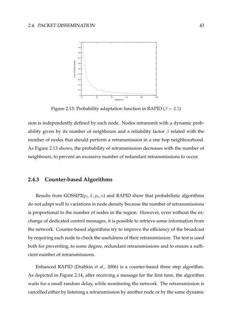
2.4. PACKET DISSEMINATION 43
0
0.1
0.2
0.3
0.4
0.5
0.6
0.7
0.8
0.9
1
0 20 40 60 80 100
Pro
b of
Ret
rans
mis
sion
Neighbours
Figure 2.13: Probability adaptation function in RAPID (β = 2.5)
sion is independently defined by each node. Nodes retransmit with a dynamic prob-
ability given by its number of neighbours and a reliability factor β related with the
number of nodes that should perform a retransmission in a one hop neighbourhood.
As Figure 2.13 shows, the probability of retransmission decreases with the number of
neighbours, to prevent an excessive number of redundant retransmissions to occur.
2.4.3 Counter-based Algorithms
Results from GOSSIP2(p1, k, p2, n) and RAPID show that probabilistic algorithms
do not adapt well to variations in node density because the number of retransmissions
is proportional to the number of nodes in the region. However, even without the ex-
change of dedicated control messages, it is possible to retrieve some information from
the network. Counter-based algorithms try to improve the efficiency of the broadcast
by requiring each node to check the usefulness of their retransmission. The test is used
both for preventing, to some degree, redundant retransmissions and to ensure a suffi-
cient number of retransmissions.
Enhanced RAPID (Drabkin et al., 2006) is a counter-based three step algorithm.
As depicted in Figure 2.14, after receiving a message for the first time, the algorithm
waits for a small random delay, while monitoring the network. The retransmission is
cancelled either by listening a retransmission by another node or by the same dynamic

44 CHAPTER 2. RELATEDWORK
Uses:NNEIGH: current estimated number of neighboursβ: reliability factords: small maximum timer delaydl: large maximum timer delay
1: msgSet← {}
2: upon event RECEIVE(msg) do3: ifmsg 6∈ msgSet then4: DELIVER(msg)5: msgSet← msgSet
⋃
{msg}6: d←RANDOM(0,ds)
7: p← min{
1, β
NNEIGH
}
8: SETALARM(d,{msg,p})9: else10: CANCELALARM(msg)11: end if12: end upon
13: upon event ALARM({msg,p}) do14: if RANDOM(0,1)<p then15: SEND(msg)16: else17: d←RANDOM(0,dl)18: SETALARM(d,{msg,1.0})19: end if20: end upon
Figure 2.14: Enhanced RAPID algorithm
probability function used in RAPID (see Section 2.4.2). However, a node that decides
not to retransmit continues to monitor the network for an additional random time.
This second monitoring period has a larger interval. The node will retransmit with
probability 1 if it does not listen at least one retransmission of the message during this
period.
Like in GOSSIP1(p, k), in GOSSIP3(p, k,m) when a node receives a message for the
first time, it will retransmit it with probability p, with p = 1 if the source is less than k
hops away. However, each node that decided not to retransmit is required to confirm
that a sufficient number (m) of retransmissions occurs so that the broadcast does not
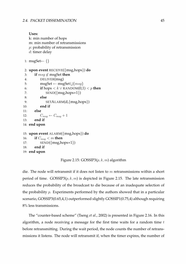
2.4. PACKET DISSEMINATION 45
Uses:k: min number of hopsm: min number of retransmissionsp: probability of retransmissiond: timer delay
1: msgSet← {}
2: upon event RECEIVE({msg,hops}) do3: ifmsg 6∈ msgSet then4: DELIVER(msg)5: msgSet← msgSet
⋃
{msg}6: if hops < k ∨ RANDOM(0,1) < p then7: SEND({msg,hops+1})8: else9: SETALARM(d,{msg,hops})10: end if11: else12: Cmsg ← Cmsg + 113: end if14: end upon
15: upon event ALARM({msg,hops}) do16: if Cmsg < m then17: SEND({msg,hops+1})18: end if19: end upon
Figure 2.15: GOSSIP3(p, k,m) algorithm
die. The node will retransmit if it does not listen to m retransmissions within a short
period of time. GOSSIP3(p, k,m) is depicted in Figure 2.15. The late retransmission
reduces the probability of the broadcast to die because of an inadequate selection of
the probability p. Experiments performed by the authors showed that in a particular
scenario, GOSSIP3(0.65,4,1) outperformed slightly GOSSIP1(0.75,4) although requiring
8% less transmissions.
The “counter-based scheme” (Tseng et al., 2002) is presented in Figure 2.16. In this
algorithm, a node receiving a message for the first time waits for a random time t
before retransmitting. During the wait period, the node counts the number of retrans-
missions it listens. The node will retransmit if, when the timer expires, the number of

46 CHAPTER 2. RELATEDWORK
Uses:m: min number of retransmissionsmaxDelay: maximum delay
1: msgSet← {}
2: upon event RECEIVE(msg) do3: ifmsg 6∈ msgSet then4: DELIVER(msg)5: msgSet← msgSet
⋃
{msg}6: delay←RANDOM(0,maxDelay)7: SETALARM(delay,msg)8: else9: Cmsg ← Cmsg + 110: end if11: end upon
12: upon event ALARM(msg) do13: if Cmsg < m then14: SEND(msg)15: end if16: end upon
Figure 2.16: Counter-based scheme
retransmissions listened is below a predefined threshold value.
Like in GOSSIP3(p, k,m), nodes in the “counter-based scheme” count the num-
ber of retransmissions listened to decide if they should retransmit. However, in
the “counter-based scheme” the transmissions are distributed over some time pe-
riod. This may be advantageous for wireless networks as it reduces the number
of collisions in multiple access MAC protocols like the IEEE 802.11 (IEEE 802.11,
1999). These algorithms differ also in the expected number of retransmissions, which
in GOSSIP3(p, k,m) depends of the network density but is a fixed constant in the
“counter-based scheme”.
In the “Hop Count-Aided Broadcasting” (HCAB) algorithm (Huang et al., 2006),
messages carry an hop count field (HC) set to zero by the source and incremented at
every retransmission. As depicted in Figure 2.17, nodes receiving the message for the
first time start a random timer and record the value of HC. Themessage will be retrans-

2.4. PACKET DISSEMINATION 47
Uses:maxDelay: maximum delay
1: msgSet← {}
2: upon event RECEIVE({msg,HC}) do3: ifmsg 6∈ msgSet then4: DELIVER(msg)5: msgSet← msgSet
⋃
{msg}6: HCmsg ← HC7: delay←RANDOM(0,maxDelay)8: SETALARM(delay,msg)9: else10: if HC > HCmsg then11: CANCELALARM(msg)12: end if13: end if14: end upon
15: upon event ALARM(msg) do16: SEND({msg,HCmsg + 1})17: end upon
Figure 2.17: Hop Count-Aided Broadcasting algorithm
mitted by the node if, when the timer expires, no message with an HC higher than the
first was received. Implicitly, nodes in HCAB try to assure that each transmission is
forwarded by some node, hopefully covering additional regions of the network.
2.4.4 Distance-Aware Algorithms
When nodes are equipped with omni-directional antennas, each transmission per-
formed by a node S is propagated in every direction. The signal strength fades with the
distance to the source by a factor that depends of different physical aspects, such as ob-
stacles traversed by the signal. The transmission of a message by S will be received by
a node R if at R’s location the signal strength is above the minimum receiving thresh-
old of R’s interface. A simplified theoretical model commonly used in the literature
assumes that nodes are homogeneous. That is, all nodes transmit with the same power

48 CHAPTER 2. RELATEDWORK
������������������������������������������������������������������������������������������������������������������������������������������������������������������������������������������������������������������������������������������������������������������������������������������������
������������������������������������������������������������������������������������������������������������������������������������������������������������������������������������������������������������������������������������������������������������������������������������������������
S R
rr
(a) Small additionalcoverage
������������������������������������������������������������������������������������������������������������������������
������������������������������������������������������������������������������������������������������������������������
S R
rr
(b) Maximum additional cov-erage
Figure 2.18: Overlap of the coverage of the transmission range between two nodes
and have an equal minimum receiving threshold. It is also assumed that there is a
monotonously decreasing function that maps the distance to the source in the signal
strength.
In this model, the receivers of any message transmitted by some node S are those
lying within a circle centred at S and with a radius that depends of the transmission
power, the fading of the signal and the minimal reception threshold. If all these factors
are known, it is possible to map the power with which each message is received by
some node on its distance to the source. This section uses the model above to present
some algorithms that use the distance between the nodes as a criteria for the selection
of the nodes that will retransmit a message.
A node R that retransmits a message must have received it from some node S.
Therefore, R must be within transmission range of S. Since it is assumed that nodes
use omni-directional antennas, part of the coverage provided by the retransmission of
R will overlap with the region previously covered by the transmission from S. Fig-
ure 2.18 illustrates this by presenting two nodes S andR and their transmission ranges
as circles of radius r.
For the theoretical model presented above, it was shown in (Tseng et al., 2002) that
the additional coverage provided by a retransmission may increase between 0% and
61% the coverage of the previous retransmission. Figures 2.18(a) and 2.18(b) show
the additional coverage provided with a retransmission by R and the overlapped re-
gion. As it can be seen, the gains depend of the location of the node performing the

2.4. PACKET DISSEMINATION 49
Uses:maxPwr: threshold transmission powermaxDelay: maximum delay
1: msgSet← {}
2: upon event RECEIVE(msg,P) do3: ifmsg 6∈ msgSet then4: DELIVER(msg)5: msgSet← msgSet
⋃
{msg}6: Pmsg ← P7: delay←RANDOM(0,maxDelay)8: SETALARM(delay,msg)9: else10: Pmsg ← max {Pmsg,P}11: end if12: end upon
13: upon event ALARM(msg) do14: if Pmsg < maxPwr then15: SEND(msg)16: end if17: end upon
Figure 2.19: Distance-based scheme
retransmission: a node closer to the source (Figure 2.18(a)) contributes with a smaller
additional coverage and a node more distant to the source (Figure 2.18(b)) with an
higher additional coverage.
Preventing nodes too close to a previous sender (and therefore providing a negli-
gible contribution to the coverage) from retransmitting is addressed in the “distance-
based scheme” described in (Tseng et al., 2002) and depicted in Figure 2.19. After re-
ceiving a message, nodes set a timer for a random time. During this period, nodes
computeM , the maximum received signal strength (RSSI) of the original message and
of all copies. A node will retransmit a message only if when the timer expiresM does
not exceed a predefined threshold.
Given that in the wireless media the signal strength decays with the distance to
the sender, it can also be said that this model prevents nodes within a minimal dis-

50 CHAPTER 2. RELATEDWORK
tance from a previous sender from forwarding the message. Like in the counter-based
algorithms presented in Section 2.4.3, the “distance-based scheme” adapts well to dif-
ferent network densities: the number of transmissions does not grow with the average
number of neighbours.
In the “Self-Adaptive Probability Broadcasting” (SAPB) (Huang et al., 2006), the
probability of a node to retransmit a message is given by an aggregation of three met-
rics. Figure 2.20 shows that like in many other algorithms described above, each node
sets a timer for a random time after receiving a message for the first time. When the
timer expires, the probability of retransmission will be given by:
P = K.f(n).g(Sx) (2.2)
where K is a constant defined so that 0 < P ≤ 1, n is the number of transmissions
received and Sx is the maximum of the Received Signal Strength Indicator (RSSI) of
all copies of the message received during the time interval. Functions f(n) and g(Sx)
should bemonotonously decreasing so that the probability of retransmission decreases
with the number of retransmissions listened and with their RSSI. SAPB combines the
three major topics that have been addressed in the other proposals discussed: a ran-
dom selection of the nodes, a bound on the number of retransmissions in the neigh-
bourhood of each node and a bound on the distance to the source of previous trans-
missions.
2.4.5 Discussion
A summary of the key characteristics of each algorithm discussed in this section
is presented on Table 2.2. The column “bounded transmissions” shows which algo-
rithms impose an absolute limit on the number of retransmissions in the neighbour-
hood of each node. This is an important aspect as it evaluates the adaptation of the
algorithms to different node densities. Of the surveyed algorithms, only the Enhanced
RAPID and “Counter-based scheme” prevent a node from retransmitting if it listens

2.4. PACKET DISSEMINATION 51
Uses:K: constant multiplicative factorf: function over the number of retransmissionsg: function over maximum transmission powermaxDelay: maximum delay
1: msgSet← {}
2: upon event RECEIVE(msg,P) do3: ifmsg 6∈ msgSet then4: DELIVER(msg)5: msgSet← msgSet
⋃
{msg}6: Nmsg ← 17: Smsg ← P8: delay←RANDOM(0,maxDelay)9: SETALARM(delay,msg)10: else11: Nmsg ← Nmsg + 112: Smsg ← max {Smsg,P}13: end if14: end upon
15: upon event ALARM(msg) do16: p← K.f(Nmsg).g(Smsg)17: if RANDOM(0,1) < p then18: SEND(msg)19: end if20: end upon
Figure 2.20: Self-Adaptive Probability Broadcasting Algorithm
to more than a predefined number of retransmissions. The “distance-based scheme”
indirectly implies an upper bound on the number of retransmissions because a trans-
mission from a node implicitly prohibits those closer than a predefined distance from
retransmitting. A lower bound can be defined as a configuration parameter (this is the
case in GOSSIP3(p, k,m) and “counter-based scheme”) or be implicit (like in HCAB) by
having the nodes to retransmit if, when its timer expires, the retransmissions listened
do not satisfy some condition.
The “source aware” column shows the algorithms that identify a potential threat to
the broadcast at the early stages of the dissemination. Indirectly, this is also addressed

52 CHAPTER 2. RELATEDWORK
AlgorithmBounded
transmissionsSourceaware
ProgressCollisionavoidance
Randomselectionof nodesUpper Lower
Probab
GOSSIP1(p) •GOSSIP1(p, k) • •GOSSIP2(p1, k, p2, n) • •RAPID •
Count Enhanced RAPID • • ◦ • •
GOSSIP3(p, k,m) • • •Count-based • • ◦ • •HCAB ◦ ◦ • • •
Dist Distance-based ◦ • • •
SAPB • ••: feature of the algorithm ◦: implicitly provided
Table 2.2: Comparison of the broadcast algorithms surveyed
by all algorithms imposing a lower bound on the number of retransmissions because
this bound is also applicable in the neighbourhood of the source.
The “Distance-based scheme” and HCAB are the two algorithms that use the ex-
pectations of additional coverage in the selection of the nodes that will retransmit. The
former by estimating the distance to the source of the previous retransmissions while
the later uses a counter that compares the original reception of the message at the node
with other retransmissions performed in the neighbourhood.
Algorithms marked in the “collision avoidance” column are those that incorporate
a mechanism to separate the retransmissions performed by the nodes, using a random
delay locally decided at each node. This separation is fundamental in some medium
access protocols to prevent contention and an undesirable number of collisions result-
ing from the simultaneous retransmission of the message by multiple nodes in a neigh-
bourhood as a result of the reception of the same message. It should be noted that any
of the other algorithms can be easily adapted to address this issue by applying some
random delay before performing the retransmission of the message.
Although with some variations, all the algorithms surveyed use randomisation to
select the nodes that will perform the retransmission. The random selection may be ex-
plicit, like in GOSSIP algorithms where nodes peek a random number to decide if they

2.5. SUMMARY 53
retransmit, or can be implicit. In these, after receiving a message, each node chooses a
random delay, and decides to retransmit at the end of the delay if some criteria has not
been satisfied by previous retransmissions. Therefore, a node that randomly selected a
smaller delay is more likely to be required to retransmit.
Contrary to the remaining, RAPID, Enhanced RAPID and GOSSIP2(p1, k, p2,m)
adapt their probability of retransmission to the local node density. The former two us-
ing a linear variation and the later with a fixed threshold. This is an interesting feature,
which, although not explicitly bounding the number of retransmissions attempts to
adapt to the network conditions in the neighbourhood of each node.
HCAB and Enhanced RAPID prevent all nodes listening to one retransmission
from sending. This is a restrictive threshold that is based on the results presented
in (Tseng et al., 2002) that concluded that very limited additional coverage is gained
with the second retransmission. As Section 3.3 will show, simulations of HCAB do not
provide a delivery ratio comparable with other algorithms using an higher threshold.
However, it should be noted that RAPID runs in the background a gossip algorithm
allowing nodes to learn and retrieve messages they did not receive with the dissemi-
nation algorithm.
2.5 Summary
Data distribution protocols can be decomposed in different modules. The decom-
position proposed in this chapter uses threemodules: local storage spacemanagement,
data management and packet dissemination. From the survey of the related work for
each of these topics we extract the following conclusions.
Cache management policies that have proven to be successful in other domains are
not themost adequate to wireless networks. However, nomain trend in customised so-
lutions has been found. Apparently, the most adequate policy is likely to depend of the
application scenario and of the particularities of the wireless networking environment.

54 CHAPTER 2. RELATEDWORK
Data management uses replication algorithms to improve resilience to faults like
disconnection, interference and device failure. In addition, replication contributes to
reduce the number of messages and bandwidth required for data retrieval.
Two major types of replication algorithms have been found. In proactive replica-
tion, data is pushed to a subset of the nodes in the network, regardless of their interest
on that particular item. In non-proactive algorithms, nodes store the data they have
previously requested or forwarded and make it available to other nodes.
A particular variant tries to evenly distribute the replicas over the entire networked
region. It was argued that geographically distribution of the replicas provides the
biggest tolerance to failures. In scenarios where the access pattern of the nodes to
the data is not correlated with their location, geographical distribution can equally
contribute to reduce the access latency and the number of messages required to re-
trieve the data. To the extent of our knowledge, proactive geographical distribution of
the data has only been pursued in the context of wireless networks where the nodes
are aware of their location. In networks where devices do not have location informa-
tion available, geographical distribution has been addressed in a limited scope, where
neighbouring nodes cooperate to prevent an excessive redundancy of the data.
To replicate data, nodes exchange messages. The survey identified four mes-
sage passing mechanisms: point-to-point, randomwalk, opportunistic gossipping and
broadcast. A correlation between point-to-point message passing and dissemination
algorithms were nodes are aware of the location of at least one copy of the items was
found. In the remaining algorithms no clear trend can be identified.
Broadcast has been widely used by protocols for wireless networks and is one of
the cornerstones of different point-to-point routing protocols for MANETs. Therefore,
a reduction on the number of messages transmitted on each broadcast contributes to
the reduction of the cost of different data dissemination protocols, including some of
those using point-to-point messages. Different proposals have recently emerged to
reduce the cost of broadcast operations. The survey showed that although implement-
ing different policies, all randomly select some of the neighbours of the source of the

2.5. SUMMARY 55
previous transmission.

56 CHAPTER 2. RELATEDWORK
3A PowerAware
Broadcasting Algorithm
Section 2.4 presented different algorithms for message dissemination that generate
a much smaller number of retransmissions than flooding. The goal of these algorithms
is to devise, in run-time, a subset of participants that are required to retransmit so
that every node in the network receives at least one copy of the message. Due to the
movement of the nodes and to the different location of the sources, this subset may be
different for each message.
An important factor to improve the performance of broadcast algorithms for
MANETs and which has been previously neglected in the literature is the location
of the nodes performing a retransmission with respect to the source of the previous
transmissions. We provide a simple case study supporting this claim.
Figure 3.1 represents a region of a MANET with a source S of a broadcast message
and its neighbours. It is assumed that the network follows the simplified network-
ing model described in Section 2.4.4. In brief, that all nodes transmit with the same
power and are capable of receiving a message if the signal strength at the receiver is
above some minimum threshold. The figure assumes that the transmission range of all
nodes is r and that the minimal power threshold used by the “distance-based scheme”
described in Section 2.4.4 is r′. The transmission range of nodes S,B,C and F is repre-
sented by circles.
The region covered by a retransmission of a broadcast initiated by S growswith the
distance of the retransmitting node to S. Elsewhere (Tseng et al., 2002), it was shown
57

58 CHAPTER 3. A POWER-AWARE BROADCASTING ALGORITHM
r’r r rr
r’
r
G S A B C D EF
Figure 3.1: Deployment and transmission range of some nodes
that if all nodes transmit with equal power, a retransmission can increase between 0%
and 61% the space covered by the previous transmission, depending on the location
of the retransmitting node. In this example, the most efficient retransmissions would
be performed by nodes C and F . The minimal number of transmissions required to
deliver a message broadcasted by node S to all other nodes is three: the message is
delivered to nodes A,B,C and F by the first transmission and nodes C and F could
retransmit to deliver it respectively toD and E, and G. We emphasise that, in runtime,
nodes do not have access to the information required for following the same rationale
presented above.
Section 2.4.5 showed that all algorithms surveyed in the related work randomly
select the nodes that perform a retransmission. Applying these algorithms to the sce-
nario depicted in Figure 3.1 shows that for all algorithms the random selection of the
nodes may result in at least four, instead of the optimal three retransmissions. With
exception of the “distance-based scheme”, all algorithms will randomly select one of
the nodes A, B or C to perform the first retransmission. The transmission by node
A, for example, satisfies the conditions of all these algorithms but provides a minimal
contribution to increase the number of nodes that received the message. Depending on
the algorithm and on its configuration parameters, a retransmission by node A would
either: i) require a retransmission by node D in order to have the message delivered
to node E, or ii) be useless, if nodes B or C retransmit as well. Therefore, if node A is
selected, the message can not be delivered to every node in the figure with less than

3.1. PAMPA 59
four transmissions.
The “Distance-based scheme” is configured with a fixed threshold. This threshold
can not be too close to the maximum transmission range to prevent the elimination
of good candidates for retransmission in the cases where nodes are not uniformly dis-
tributed. In the example of Figure 3.1, the threshold is represented using dashed circles
with radius r′ and excludes node A from the list of candidates for retransmission of a
message sent by S. However, the “distance-based scheme” does not rank differently
the nodes located outside the circle defined by r′. After the transmission by node S,
both nodes B and C are candidates to retransmit. This algorithm would require four
transmissions if the timer of node B expires before the timer of node C. It should be
noted that the retransmission by B would even inhibit node C from retransmitting.
This chapter proposes a novel algorithm to reduce the resources consumed by the
nodes and the bandwidth required by broadcasts in MANETs. This is a challenging
problem because we want to minimise the signalling overhead and we do not want to
enforce the use of special hardware (e.g. nodes are not required to use a GPS receiver
to become aware of their location). Like in the “distance-aware scheme” (Tseng et al.,
2002), our algorithm only assumes that nodes are able to retrieve the power with which
each message is received. The algorithm, named Power-Aware Message Propagation
Algorithm (Pampa) is distinguished from the previous proposals by removing some
of the randomness associated with the decision on the nodes that will retransmit a
message. Simulation results, to be presented in Section 3.3 experimentally confirm that
the selection of the nodes can be improved to prevent the occurrence of these cases.
3.1 Pampa
As mentioned before, the increment in the coverage provided by a retransmitting
node may vary between 0% and 61%. This ratio grows with the distance to the source.
The key idea of Pampa is to run a fully distributed algorithm that makes nodes more
distant to the source to retransmit first, instead of relying on the random selection of
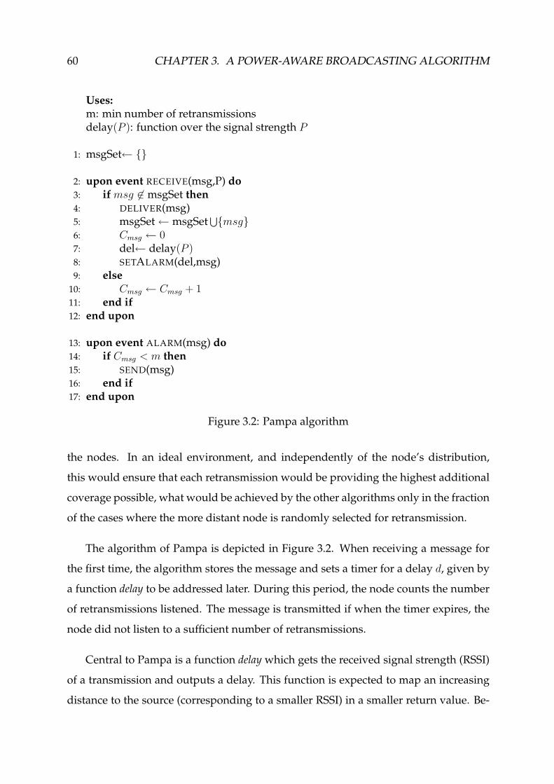
60 CHAPTER 3. A POWER-AWARE BROADCASTING ALGORITHM
Uses:m: min number of retransmissionsdelay(P ): function over the signal strength P
1: msgSet← {}
2: upon event RECEIVE(msg,P) do3: ifmsg 6∈ msgSet then4: DELIVER(msg)5: msgSet← msgSet
⋃
{msg}6: Cmsg ← 07: del← delay(P )8: SETALARM(del,msg)9: else10: Cmsg ← Cmsg + 111: end if12: end upon
13: upon event ALARM(msg) do14: if Cmsg < m then15: SEND(msg)16: end if17: end upon
Figure 3.2: Pampa algorithm
the nodes. In an ideal environment, and independently of the node’s distribution,
this would ensure that each retransmission would be providing the highest additional
coverage possible, what would be achieved by the other algorithms only in the fraction
of the cases where the more distant node is randomly selected for retransmission.
The algorithm of Pampa is depicted in Figure 3.2. When receiving a message for
the first time, the algorithm stores the message and sets a timer for a delay d, given by
a function delay to be addressed later. During this period, the node counts the number
of retransmissions listened. The message is transmitted if when the timer expires, the
node did not listen to a sufficient number of retransmissions.
Central to Pampa is a function delay which gets the received signal strength (RSSI)
of a transmission and outputs a delay. This function is expected to map an increasing
distance to the source (corresponding to a smaller RSSI) in a smaller return value. Be-

3.1. PAMPA 61
cause the RSSI will be different for each node, the function delay will return a different
value for each node receiving the same transmission. Implicitly, the function orders the
nodes according to the distance to the source, with nodes more distant to the source
expiring their timers first. It should be noted that the function is fully distributed: the
algorithm is triggered exclusively by the transmission of the broadcast message and
it does not require any coordination between the nodes. Like in the “counter-based
scheme” (Tseng et al., 2002), the algorithm prevents excessive redundancy by having
nodes to count the number of retransmissions listened. However, Pampa bias the de-
lay such that the nodes refraining from transmitting are usually those that are closer to
the source.
3.1.1 Delay Assignment
The selection of a good delay function is key to the performance of Pampa. We es-
timate that a delay function that varies linearly with the distance to the source would
provide the best results. However, such a function would require complex computa-
tions unsuitable to be performed by mobile devices for each received message.
In our tests, we defined two simpler delay functions that multiply the RSSI by a con-
stant k to return the number of seconds that the node should wait before retransmit-
ting. Analysis of an adequate value for k was performed using the Two Ray Ground
propagation model as defined in the ns–2 network simulator version 2.28. We have
found 300 × 106 to be an adequate value for obtaining distinct wait times for nodes
close to each other. The behaviour of the function delay(p) = 300× 106 × p for the Two
Ray Ground propagation model is presented in Figure 3.3.
As expected, the function follows the logarithmic decay of the reception power of
a message. For short distances, the function returns excessively large delay values.
However, nodes at these distances from the source have a large probability of not be-
ing required to retransmit. A careful implementation of the algorithm can free the
resources consumed by the messages on hold as soon as the threshold number of re-

62 CHAPTER 3. A POWER-AWARE BROADCASTING ALGORITHM
0
2
4
6
8
10
12
80 100 120 140 160 180 200 220 240 260
Del
ay (
s)
Distance to the source (m)
delay(p)delay2(p)
Figure 3.3: Function delay
transmissions is listened. Section 3.3.2.1 will show that these excessive delays do not
significantly influence the propagation of the message.
However, to better assert its impact in the performance of Pampa, a second delay
function delay2was defined. This function, also depicted in Figure 3.3 defines a maxi-
mum delay of two seconds with an additional random variation of 500ms to prevent
an excessive number of collisions.
3.2 Comparison with Related Work
In Pampa, the instant at which each node forwards a message is locally determined
from its distance to the sender. In the absence of abnormal effects on the signal prop-
agation, Pampa assures that the first nodes to perform a retransmission are those that
provide the higher possible additional coverage. In the example presented in Fig-
ure 3.1, node C would be the first to retransmit, delivering the message to both nodes
D and E. Although slightly later, node F would also be required to retransmit and
therefore, guarantee the coverage of nodeG. In this example, Pampa reduces the prob-
ability of requiring four instead of the minimal three transmissions for delivering the
message to every node.
Table 3.1 extends to Pampa the comparison of the related work of Table 2.2 (see
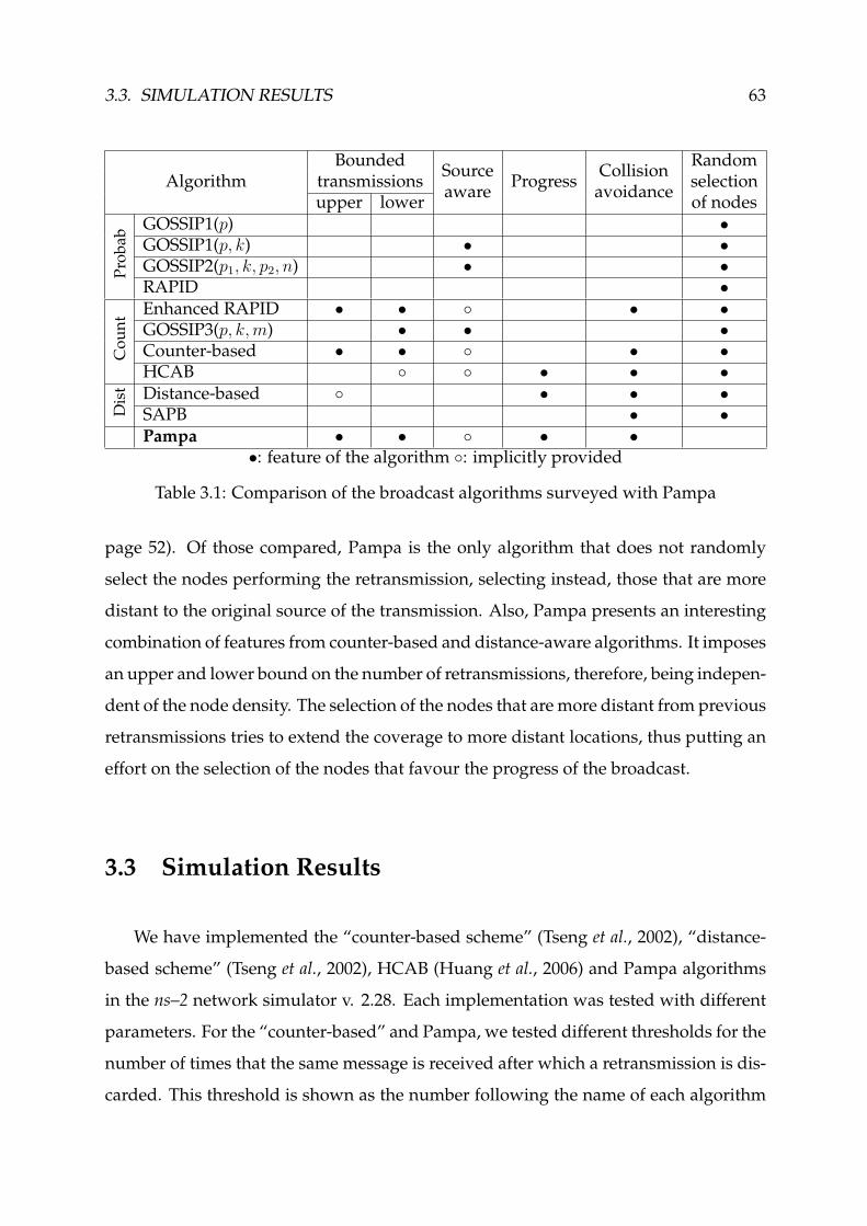
3.3. SIMULATION RESULTS 63
AlgorithmBounded
transmissionsSourceaware
ProgressCollisionavoidance
Randomselectionof nodesupper lower
Probab
GOSSIP1(p) •GOSSIP1(p, k) • •GOSSIP2(p1, k, p2, n) • •RAPID •
Count Enhanced RAPID • • ◦ • •
GOSSIP3(p, k,m) • • •Counter-based • • ◦ • •HCAB ◦ ◦ • • •
Dist Distance-based ◦ • • •
SAPB • •Pampa • • ◦ • •
•: feature of the algorithm ◦: implicitly provided
Table 3.1: Comparison of the broadcast algorithms surveyed with Pampa
page 52). Of those compared, Pampa is the only algorithm that does not randomly
select the nodes performing the retransmission, selecting instead, those that are more
distant to the original source of the transmission. Also, Pampa presents an interesting
combination of features from counter-based and distance-aware algorithms. It imposes
an upper and lower bound on the number of retransmissions, therefore, being indepen-
dent of the node density. The selection of the nodes that are more distant from previous
retransmissions tries to extend the coverage to more distant locations, thus putting an
effort on the selection of the nodes that favour the progress of the broadcast.
3.3 Simulation Results
We have implemented the “counter-based scheme” (Tseng et al., 2002), “distance-
based scheme” (Tseng et al., 2002), HCAB (Huang et al., 2006) and Pampa algorithms
in the ns–2 network simulator v. 2.28. Each implementation was tested with different
parameters. For the “counter-based” and Pampa, we tested different thresholds for the
number of times that the same message is received after which a retransmission is dis-
carded. This threshold is shown as the number following the name of each algorithm

64 CHAPTER 3. A POWER-AWARE BROADCASTING ALGORITHM
in the captions of the figures. In addition, Pampa was tested with the two delay func-
tions introduced in Section 3.1.1. In the figures that follow, Pampa with the unbound
delay function is identified as “Pampa” while Pampa using function delay2is depicted
as “Pampa2”. The “distance-based scheme” was tested with different threshold dis-
tances, identified (in meters) in the captions of the figures. HCAB does not have any
configuration parameters.
Each algorithm had some parameters immutable for all simulations. The maxi-
mum random delay used by the “counter-based scheme”, “distance-based scheme”
and HCAB was set to 0.75s. As described in Section 3.1.1, both Pampa and Pampa2
multiply the Received Signal Strength Indication (RSSI) by 300 × 106. The maximum
delay in Pampa2is 2s and the additional jitter is randomly selected between 0 and
500ms.
3.3.1 Test-bed
Different node densities have been experimented by changing the size of the simu-
lated space. Eight simulated regions were tested: 250m× 250m, 500m× 250m, 1000m×
500m, 1000m × 1000m, 2000m × 1000m, 1500m × 1500m, 2000m × 1500m and 2000m ×
2000m, providing ratios between 625m2/node and 40000m2/node. All simulations are
run with 100 nodes. Nodes were configured to emulate a 914MHz Lucent WaveLAN
DSSS radio interface running an IEEE802.11 protocol at 2Mb/s. Network cards present
a transmission range of 250m using the Two Ray Ground propagation model.
Each test combines different traffic sources and movement of the nodes. Traffic
in each test is composed of 1000 messages, generated at a pace of one message per
second. The source of each message is selected at random. The size of each message is
1000 bytes.
At the beginning of each test, nodes are uniformly deployed over the simulated
region. In one set of tests, nodes do not move for the entire duration of the simulation.
These tests have been named “Speed 0”. In the remaining two sets nodes move using

3.3. SIMULATION RESULTS 65
the Random Waypoint Movement Model (Johnson & Maltz, 1996). In this movement
model nodes select a random location in the simulated region and move in a straight
line to it at a speed randomly defined between a minimum and a maximum value.
When the location is reached, nodes stop for a predefined amount of time and initiate a
new cycle by selecting another random location. In our tests, minimum and maximum
speeds are respectively 4m/s and 6m/s for one test set and 9m/s and 11m/s for the
other. Nodes never stop. These sets have been named respectively “Speed 5” and
“Speed 10”.
For each simulated region and speed, 100 different tests were defined and experi-
mented with each of the algorithms. Each point in the figures presented below aver-
ages the result of the 100 runs. The evaluation will focus on four metrics: the propor-
tion of nodes receiving each message; the number of transmissions used; the latency of
the delivery and the number of hops required to deliver the message to the nodes.
3.3.2 Delivery Ratio
This section evaluates the efficiency of the algorithms. The metric used is the aver-
age of the proportion of the nodes that receive each message. Figure 3.4 compares the
performance of the counter based algorithms with Pampa. A comparison between the
three plots of the figure shows that the performance of all algorithms improveswith the
movement of the nodes. This behaviour is attributed to a reduced number of partitions,
which results from the concentration of nodes at the centre of the simulated space. This
is a well-known effect of the random way-point movement model (Bettstetter et al.,
2003). This conclusion is supported by counts of the average number of nodes receiv-
ing each message in the 2000m × 2000m tests. The values were of 4.30, 5.91 and 5.92
respectively for tests in Speeds 0, 5 and 10.
The figure shows that for high densities, all the algorithms are capable of delivering
every message to all nodes. As the area of the simulation increases, so does the average
distance between the nodes and the gains provided by Pampa becomemore clear. This
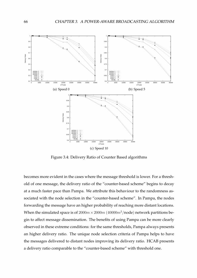
66 CHAPTER 3. A POWER-AWARE BROADCASTING ALGORITHM
0.2
0.3
0.4
0.5
0.6
0.7
0.8
0.9
1
0 5000 10000 15000 20000 25000 30000 35000 40000
Del
iver
y R
atio
m2/node
pampa, 1pampa, 2pampa, 3
count, 1count, 2count, 3
HCAB
(a) Speed 0
0.6
0.65
0.7
0.75
0.8
0.85
0.9
0.95
1
0 5000 10000 15000 20000 25000 30000 35000 40000
Del
iver
y R
atio
m2/node
pampa, 1pampa, 2pampa, 3
count, 1count, 2count, 3
HCAB
(b) Speed 5
0.6
0.65
0.7
0.75
0.8
0.85
0.9
0.95
1
0 5000 10000 15000 20000 25000 30000 35000 40000
Del
iver
y R
atio
m2/node
pampa, 1pampa, 2pampa, 3
count, 1count, 2count, 3
HCAB
(c) Speed 10
Figure 3.4: Delivery Ratio of Counter Based algorithms
becomes more evident in the cases where the message threshold is lower. For a thresh-
old of one message, the delivery ratio of the “counter-based scheme” begins to decay
at a much faster pace than Pampa. We attribute this behaviour to the randomness as-
sociated with the node selection in the “counter-based scheme”. In Pampa, the nodes
forwarding the message have an higher probability of reaching more distant locations.
When the simulated space is of 2000m×2000m (40000m2/node) network partitions be-
gin to affect message dissemination. The benefits of using Pampa can be more clearly
observed in these extreme conditions: for the same thresholds, Pampa always presents
an higher delivery ratio. The unique node selection criteria of Pampa helps to have
the messages delivered to distant nodes improving its delivery ratio. HCAB presents
a delivery ratio comparable to the “counter-based scheme” with threshold one.

3.3. SIMULATION RESULTS 67
The delivery ratio of the “distance-based scheme” with thresholds corresponding
to 125m, 175m and 225m (respectively, 50%, 70% and 90% of the transmission range)
is compared with Pampa in Figure 3.5. The figure shows that the “distance-based”
scheme is particularly sensitive to its threshold. The “distance-based scheme” exhibits
less tolerance to lower node densities than Pampa. Again, this behaviour can be par-
tially attributed to the random selection of nodes. In sparse networks, each message is
received by a small number of nodes. The propagation of the broadcast is affected if
either, all nodes receiving the message are closer to the source than the minimal thresh-
old or if the node whose timer expires first is one of the nodes closer to the source. It
should be noted that in this case, the retransmission by this node is likely to prevent the
retransmission from other nodes whose additional contribution to the coverage space
could be higher. Due to their poor performance, the rest of the evaluation omits results
for the “distance-based scheme” with thresholds corresponding to 225m and 175m.
Figure 3.6 presents a more conclusive comparison between the two best per-
forming algorithms presented before: Pampa and the “counter-based scheme”. Fig-
ures 3.6(a), 3.6(b) and 3.6(c) divide the delivery ratio of Pampa by the delivery ratio of
the “counter-based scheme” for the same threshold. Results clearly show the benefits
of using Pampa. In lowest densities, Pampa is capable of delivering up to 30% more
messages than the “counter-based scheme”. The “counter-based scheme” outperforms
Pampa only in a few densities and speeds and always with marginal gains.
It is interesting to notice that the gains increase for lower thresholds. This be-
haviour is attributed to the fact that, with higher thresholds, the probability of the
“counter-based scheme” to select the most adequate nodes for retransmission in-
creases, while Pampa tends to select these nodes even when the threshold is low. This
conclusion is supported by the results presented in Figure 3.6(d) which divide the de-
livery ratio with a threshold of 4 by the delivery ratio with a threshold of 3. The figure
shows that the “counter-based scheme” is the one that most benefits from the increased
redundancy.
The overlap between the lines for Speeds 5 and 10 is due to the similar number

68 CHAPTER 3. A POWER-AWARE BROADCASTING ALGORITHM
0
0.1
0.2
0.3
0.4
0.5
0.6
0.7
0.8
0.9
1
0 5000 10000 15000 20000 25000 30000 35000 40000
Del
iver
y R
atio
m2/node
pampa, 1pampa, 2pampa, 3
distance, 125distance, 175distance, 225
(a) Speed 0
0.1
0.2
0.3
0.4
0.5
0.6
0.7
0.8
0.9
1
0 5000 10000 15000 20000 25000 30000 35000 40000
Del
iver
y R
atio
m2/node
pampa, 1pampa, 2pampa, 3
distance, 125distance, 175distance, 225
(b) Speed 5
0.1
0.2
0.3
0.4
0.5
0.6
0.7
0.8
0.9
1
0 5000 10000 15000 20000 25000 30000 35000 40000
Del
iver
y R
atio
m2/node
pampa, 1pampa, 2pampa, 3
distance, 125distance, 175distance, 225
(c) Speed 10
Figure 3.5: Delivery Ratio of Distance Based algorithms
of neighbours counted in these simulations. A second conclusion to be derived from
Figure 3.6(d) is that independently of the network density and speed, in general, the
increment of the threshold above 3 provides only marginal gains in the delivery ratio
(below 4%). This is an important conclusion, given that it provides an upper bound
on the number of retransmissions and therefore, on the battery consumption required
for broadcast delivery. However, results presented before have shown that smaller
thresholds present considerably lower delivery ratios when the density increases.
3.3.2.1 Impact of the bounded delay
A similar comparison between Pampa and Pampa2is presented in Figure 3.7. Re-
call from Section 3.1.1 that the only difference between these algorithms is that in

3.3. SIMULATION RESULTS 69
0.95
1
1.05
1.1
1.15
1.2
1.25
1.3
0 5000 10000 15000 20000 25000 30000 35000 40000
Gai
ns
m2/node
pampa/count, 1pampa/count, 2pampa/count, 3pampa/count, 4
(a) Speed 0
0.98
1
1.02
1.04
1.06
1.08
1.1
1.12
1.14
1.16
1.18
0 5000 10000 15000 20000 25000 30000 35000 40000
Gai
ns
m2/node
pampa/count, 1pampa/count, 2pampa/count, 3pampa/count, 4
(b) Speed 5
0.98
1
1.02
1.04
1.06
1.08
1.1
1.12
1.14
1.16
1.18
1.2
0 5000 10000 15000 20000 25000 30000 35000 40000
Gai
ns
m2/node
pampa/count, 1pampa/count, 2pampa/count, 3pampa/count, 4
(c) Speed 10
1
1.005
1.01
1.015
1.02
1.025
1.03
1.035
1.04
20000 25000 30000 35000 40000
Gai
ns
m2/node
Pampa, Speed 0Pampa, Speed 5
Pampa, Speed 10Count, Speed 0Count, Speed 5
Count, Speed 10
(d) Gains using threshold 4 over threshold 3
Figure 3.6: Comparison of the delivery ratio of Pampa with the “counter-basedscheme”
Pampa2, nodes closer than 120m (approximately) to the source are randomly sorted
by the jitter delay. Therefore, Pampa2should consume less memory of the mobile de-
vices than Pampa because messages will be holden for a smaller period of time. The
figure shows that in general, Pampa slightly outperforms Pampa2by small margins
that do not exceed 1.6%. Such a small value shows that Pampa2can be used as a less
resource demanding version of Pampa without significantly reducing its performance.
The highest improvements of Pampa are for the less dense networks what confirms
the relevance of the node sorting operation performed by Pampa, even when nodes
are close to the source.

70 CHAPTER 3. A POWER-AWARE BROADCASTING ALGORITHM
0.998
0.999
1
1.001
1.002
1.003
1.004
1.005
1.006
0 5000 10000 15000 20000 25000 30000 35000 40000
Gai
ns
m2/node
pampa/pampa2, 1pampa/pampa2, 2pampa/pampa2, 3pampa/pampa2, 4
(a) Speed 0
0.999
1
1.001
1.002
1.003
1.004
1.005
1.006
1.007
1.008
1.009
1.01
0 5000 10000 15000 20000 25000 30000 35000 40000
Gai
ns
m2/node
pampa/pampa2, 1pampa/pampa2, 2pampa/pampa2, 3pampa/pampa2, 4
(b) Speed 5
0.998
1
1.002
1.004
1.006
1.008
1.01
1.012
1.014
1.016
0 5000 10000 15000 20000 25000 30000 35000 40000
Gai
ns
m2/node
pampa/pampa2, 1pampa/pampa2, 2pampa/pampa2, 3pampa/pampa2, 4
(c) Speed 10
Figure 3.7: Comparison of the delivery ratio of Pampa with Pampa2
3.3.3 Number of Transmissions
The ratio of messages sent per node and per broadcast is depicted in Figure 3.8. To
make the figures more readable, we omit to depict the results for the algorithms that
exhibit very low reliability values.
All algorithms exhibit a similar pattern, even if the absolute values differ. The
decay in the number of messages, depicted in Figure 3.8(a), is again attributed to net-
work partitions which are less likely to occur when nodes move. Nodes in a partition
other than the one where the sending node is located are unable to receive the message
and therefore, can not retransmit it. Pampa and the “counter-based scheme” use the
same algorithm at each node for deciding whether to retransmit or not. Therefore, for
the same threshold, both algorithms present a similar number of messages. However,

3.3. SIMULATION RESULTS 71
0
0.1
0.2
0.3
0.4
0.5
0.6
0.7
0.8
0 5000 10000 15000 20000 25000 30000 35000 40000
Mes
sage
s se
nt/N
ode/
Bro
adca
st
m2/node
pampa, 2pampa, 3pampa, 4
pampa2, 2pampa2, 3pampa2, 4
count, 2count, 3count, 4
distance, 125HCAB
(a) Speed 0
0
0.1
0.2
0.3
0.4
0.5
0.6
0.7
0 5000 10000 15000 20000 25000 30000 35000 40000
Mes
sage
s se
nt/N
ode/
Bro
adca
st
m2/node
pampa, 2pampa, 3pampa, 4
pampa2, 2pampa2, 3pampa2, 4
count, 2count, 3count, 4
distance, 125HCAB
(b) Speed 5
0
0.1
0.2
0.3
0.4
0.5
0.6
0.7
0 5000 10000 15000 20000 25000 30000 35000 40000
Mes
sage
s se
nt/N
ode/
Bro
adca
st
m2/node
pampa, 2pampa, 3pampa, 4
pampa2, 2pampa2, 3pampa2, 4
count, 2count, 3count, 4
distance, 125HCAB
(c) Speed 10
Figure 3.8: Transmissions ratio
it was shown before that Pampa achieves an higher delivery ratio, what justifies the
small increment in the number of messages transmitted for low node densities.
The figure also confirms the advantages of the counter based and distance aware
algorithms over pure probabilistic ones. The GOSSIP algorithms presented in (Haas
et al., 2002) required a probability of retransmission above 60% to ensure an high prob-
ability of delivery to every node. Our experiments suggest that such a high retrans-
mission rate is only required for sparse networks, where the number of neighbours is
low.

72 CHAPTER 3. A POWER-AWARE BROADCASTING ALGORITHM
0
1
2
3
4
5
6
0 5000 10000 15000 20000 25000 30000
Hop
s
m2/node
pampa, 2pampa, 3
count, 2count, 3
distance, 125HCAB
Figure 3.9: Hops to the source of the message (Speed 0)
3.3.4 Coverage
In principle, the criteria used for selecting retransmitting nodes in Pampa should
improve the utility of each retransmission, measured by the number of nodes receiving
amessage for the first timewith each retransmission. To confirm this intuition, we have
counted, for each message, the number of hops travelled until it is delivered for the
first time to each node. The results are presented in Figure 3.9, which omits the results
for the networks with 2000m× 2000m because it was considered that the low delivery
ratio presented does not allow the interpretation of this metric. The figure shows that
Pampa delivers messages in less hops than the remaining algorithms, confirming the
utility gains expected for Pampa.
The figure also shows that contrary to the “counter based scheme”, the number of
hops in Pampa is independent of the threshold. This behaviour is attributed to the ran-
domness of the “counter-based scheme”: when its threshold is lower, the probability of
having the most adequate nodes selected is reduced and some nodes will only receive
the message after an additional retransmission. This conclusion is also supported by
the good performance of the “distance-based scheme” in this metric. By prohibiting
nodes too close to the source from retransmitting, the algorithm inherently favours the
selection of the nodes that are capable of providing the highest coverage. On the con-
trary, the random selection of the nodes that retransmit in HCAB does not provide any
guarantee that the node that retransmits will provide a good additional coverage.

3.4. SUMMARY 73
0
0.5
1
1.5
2
2.5
0 5000 10000 15000 20000 25000 30000
Del
ay (
s)
m2/node
pampa, 2pampa, 3
pampa2, 2pampa2, 3
count, 2count, 3
distance, 125HCAB
Figure 3.10: Average latency (Speed 0)
3.3.5 Delay
To conclude the evaluation, Figure 3.10 presents the average time interval between
the initial transmission of a message and its delivery to each node. Results show that
for high densities, messages in Pampa have a latency comparable with the remaining
algorithms.
In sparse networks, the difference between Pampa and the remaining algorithms
becomes significant. However, as shown before, it is in these networks that Pampa
more significantly outperforms the remaining algorithms. Results for Pampa2high-
light an implicit trade-off of Pampa: an excessive delay can be mitigated using a delay
function that puts an upper bound on the delay of each nodes. However, as shown in
Section 3.3.2.1, a lower latency implies a small degradation in the delivery ratio.
3.4 Summary
In Mobile Ad Hoc Networks, broadcasting a message to every node is an oper-
ation that consumes a non-negligible amount of resources at all participants. How-
ever, broadcast is a basic mechanism often required by protocols at different levels of
the network stack. The most simple implementation of broadcast consists in having
each node to retransmit each message after receiving it for the first time. This imple-

74 CHAPTER 3. A POWER-AWARE BROADCASTING ALGORITHM
mentation, usually referred as flooding, creates a large redundancy of messages in the
network and unnecessarily wastes resources at the participating nodes.
This chapter presented a new algorithm that uses information locally available at
each node to reduce the redundancy of the broadcast operation. The novelty of the
algorithm, named Pampa, is the ranking of the nodes according to their distance to
the source. Pampa does not require the exchange of control messages or specialised
hardware.
The algorithm was compared with previous proposals and it was shown to im-
prove their performance, particularly in more adverse conditions like sparse networks,
at the expenses of a small increase in the latency of the delivery.

4Replica Management
Chapter 2 surveyed different data dissemination and retrieval algorithms designed
for a large variety of networking models. We have observed that some dissemination
algorithms attempt to place the replicas in a geographically distributed manner. There
are two main reasons to promote a geographical distribution of the replicas:
Improved resilience to failures. If replicas are geographically distributed, the proba-
bility of having all of them being affected by some localised malfunction of the
network, such as interference, is reduced. If the network becomes partitioned,
geographical distribution may also increase the probability of having replicas
available in the different partitions of the network.
Decreased cost of data retrieval. Assuming that there is no relation between the loca-
tion of the nodes and the data they query, geographical distribution of the repli-
cas reduces both the cost (in number of messages) and the time to access the data,
because the probability of finding the data item in some close neighbour of the
client increases.
Algorithms that promote a geographical distribution of replicas have been de-
signed under different assumptions. Some algorithms provide a limited form of ge-
ographical distribution by preventing replicas from being close to each other (Hara,
2001). Others effectively distribute the replicas but require the nodes to be aware of
their location. These alternatives have been discussed in Section 2.3.6, where we had
the opportunity to note the absence of protocols that perform a proactive geograph-
ical distribution of the replicas for scenarios where the nodes are not aware of their
75

76 CHAPTER 4. REPLICA MANAGEMENT
location. This chapter proposes to fill the gap by presenting a protocol with these char-
acteristics.
In our work, we assume that either: i) there is no predictable (biased) access pat-
tern to the objects or; ii) that this access pattern cannot be derived a priori or even dur-
ing the lifetime of the system. Therefore, we aim at distributing data items as evenly as
possible among all the nodes that form the network, avoiding clustering of information
in sub-areas. An uniform dissemination of data items should leverage access latency
to any item from any node in the network, i.e, whenever a data item is requested by a
node S, the distance to the node that provides the reply should be approximately the
same, regardless of the location of S. Naturally, the actual distance depends on mul-
tiple parameters, such as the number of nodes in the network, the amount of memory
made available at each node, and the number of data items.
The chapter is organised as follows. Section 4.1 formalises the assumptions of the
system model used by the algorithm. The protocol is described in four sections. Sec-
tion 4.2 introduces the configuration parameters and the auxiliary modules. The dis-
semination algorithm, named Power-Aware data DISsemination algorithm (PADIS) is
presented in Section 4.3. An algorithm for data retrieval well suited to the dissemina-
tion algorithm is described in Section 4.4. Section 4.5 discusses different algorithms for
correcting the data distribution in the presence of node movement. Section 4.6 analyti-
cally compares our work with the algorithms surveyed in the related work. Evaluation
was performed using a network simulator. The results are presented in Section 4.7. Fi-
nally, Section 4.8 summarises the results of the chapter.
4.1 SystemModel
Our work makes no assumption on the distribution of the nodes or on the size of
the network (both in number of nodes and dimension). Devices communicate using
omni-directional antennas and are able to establish bidirectional links. That is, if some
node A is able to receive messages from one neighbour B, then node B is also able to

4.2. INITIALISATION 77
receive messages transmitted by node A. Nodes are not aware of their location or of
the location of their neighbours.
To prevent trivial solutions to the data dissemination problem, we require the net-
work to be large enough, avoiding all nodes from being within direct communication
of each other. To be able to deliver data to every participating node, we assume that
the network density is such that partitions are rare.
Nodes are producers and consumers of a (a priori unknown) number of data items,
composed of a key and a value. The key is required to uniquely identify each data
item. The algorithm does not interpret the content or structure of the key but assumes
that the application provides a function allowing to determine if two keys are equal.
Data items are short so that a few can fit in a single frame at the link layer level. Nodes
always store the items they produce in a separate region of the memory with unlimited
size.
Nodes are required to cooperate. Nodes must adhere to the protocol by i) forward-
ing messages, ii) keeping the items they produce in memory, iii)making some storage
space permanently available for keeping data advertised by other nodes and iv) reply
whenever listening for a query for a data item they store. Typically, the storage space at
each node is enough for keeping only a fraction of the total amount of data produced.
The system model above shares many assumptions with those presented for some
of the frameworks surveyed in the related work. A remarkably similar set of assump-
tions is presented for SAF, DAFN, and DCG, although we remove the assumptions
on the predictability of the data access (Hara, 2001) and on the correlation of the
queries (Hara et al., 2004).
4.2 Initialisation
Bootstrap of the dissemination and query algorithms require the setting up of a
number of variables depicted in Figure 4.1. The same figure also presents the configu-
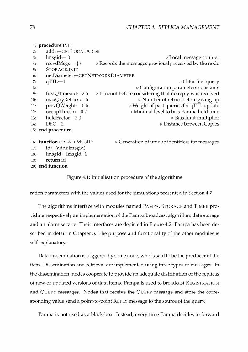
78 CHAPTER 4. REPLICA MANAGEMENT
1: procedure INIT2: addr←GETLOCALADDR3: lmsgid← 0 ⊲ Local message counter4: recvdMsgs← {} ⊲ Records the messages previously received by the node5: STORAGE.INIT6: netDiameter←GETNETWORKDIAMETER7: qTTL←1 ⊲ ttl for first query8: ⊲ Configuration parameters constants9: firstQTimeout←2.5 ⊲ Timeout before considering that no reply was received10: maxQryRetries← 5 ⊲Number of retries before giving up11: prevQWeight← 0.5 ⊲Weight of past queries for qTTL update12: occupThresh← 0.7 ⊲Minimal level to bias Pampa hold time13: holdFactor←2.0 ⊲ Bias limit multiplier14: DbC←2 ⊲ Distance between Copies15: end procedure
16: function CREATEMSGID ⊲ Generation of unique identifiers for messages17: id←(addr,lmsgid)18: lmsgid←lmsgid+119: return id20: end function
Figure 4.1: Initialisation procedure of the algorithms
ration parameters with the values used for the simulations presented in Section 4.7.
The algorithms interface with modules named PAMPA, STORAGE and TIMER pro-
viding respectively an implementation of the Pampa broadcast algorithm, data storage
and an alarm service. Their interfaces are depicted in Figure 4.2. Pampa has been de-
scribed in detail in Chapter 3. The purpose and functionality of the other modules is
self-explanatory.
Data dissemination is triggered by some node, who is said to be the producer of the
item. Dissemination and retrieval are implemented using three types of messages. In
the dissemination, nodes cooperate to provide an adequate distribution of the replicas
of new or updated versions of data items. Pampa is used to broadcast REGISTRATION
and QUERY messages. Nodes that receive the QUERY message and store the corre-
sponding value send a point-to-point REPLY message to the source of the query.
Pampa is not used as a black-box. Instead, every time Pampa decides to forward

4.2. INITIALISATION 79
Pampa
+ relay(id,msg,ttl)+ send(addr,id,msg,ttl)+ decide(id):bool+ drop(id)
Timer
+ setAlarm(time,id)
Storage
+ add(key,value)+ addLocal(key,value)+ hasValue(key):bool+ getValue(key):value+ occupRatio():real
Figure 4.2: Auxiliary modules of the distribution and query algorithms
or drop a message, it first issues a call-back: the dissemination and query algorithms
may then update the contents of the message, or overrule Pampa’s decision on the fate
of the message. In particular the algorithms may opt to force the transmission of a
message that would be otherwise dropped by Pampa.
The module PAMPA exports the methods RELAY for retransmitting a message;
DROP to discard a message; and SEND for point-to-point delivery to a node in trans-
mission range.1 The Pampa’s decision to forward or drop a message is retrieved using
the method DECIDE. Additionally, PAMPA notifies the algorithms by delivering events
when new messages or duplicates arrive. The notification includes the suggested hold
time for the message, i.e. the time the receiver should wait for other retransmissions
before relaying the message.
Data is kept in the STORAGE module. The module allows to differentiate data gen-
erated at the node (using the ADDLOCAL method) and which can not be erased from
data provided by other nodes (the ADD method) which can be overwritten by later
entries if the storage space fills. Nodes always try to keep their storage space full, oc-
cupying all free space before beginning to overwrite other entries. Each data item is
stored together with a flag replacewhose purpose will be described later.
1Point-to-point message passing is associated to PAMPA only to keep on this module all networkrelated activities.
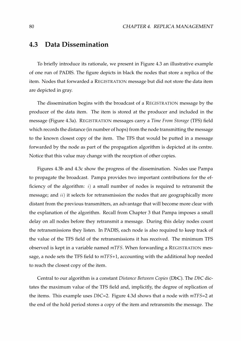
80 CHAPTER 4. REPLICA MANAGEMENT
4.3 Data Dissemination
To briefly introduce its rationale, we present in Figure 4.3 an illustrative example
of one run of PADIS. The figure depicts in black the nodes that store a replica of the
item. Nodes that forwarded a REGISTRATION message but did not store the data item
are depicted in gray.
The dissemination begins with the broadcast of a REGISTRATION message by the
producer of the data item. The item is stored at the producer and included in the
message (Figure 4.3a). REGISTRATION messages carry a Time From Storage (TFS) field
which records the distance (in number of hops) from the node transmitting themessage
to the known closest copy of the item. The TFS that would be putted in a message
forwarded by the node as part of the propagation algorithm is depicted at its centre.
Notice that this value may change with the reception of other copies.
Figures 4.3b and 4.3c show the progress of the dissemination. Nodes use Pampa
to propagate the broadcast. Pampa provides two important contributions for the ef-
ficiency of the algorithm: i) a small number of nodes is required to retransmit the
message; and ii) it selects for retransmission the nodes that are geographically more
distant from the previous transmitters, an advantage that will become more clear with
the explanation of the algorithm. Recall from Chapter 3 that Pampa imposes a small
delay on all nodes before they retransmit a message. During this delay nodes count
the retransmissions they listen. In PADIS, each node is also required to keep track of
the value of the TFS field of the retransmissions it has received. The minimum TFS
observed is kept in a variable named mTFS. When forwarding a REGISTRATION mes-
sage, a node sets the TFS field to mTFS+1, accounting with the additional hop needed
to reach the closest copy of the item.
Central to our algorithm is a constant Distance Between Copies (DbC). The DbC dic-
tates the maximum value of the TFS field and, implicitly, the degree of replication of
the items. This example uses DbC=2. Figure 4.3d shows that a node with mTFS=2 at
the end of the hold period stores a copy of the item and retransmits the message. The

4.3. DATA DISSEMINATION 81
0 0
1
1
1
1
1
a) b)
2
2
2
222
0
1
1
1
1
2
21
2
2
2
2
2
22
0
1
1
1
1
2
2
0
0
21
c) d)
2
2
2
1
2
2
0
1
1
1
1
2
1
0
0
1
11
1
1
1 12
2 12
2
2 2
2
2
2
2
0 1
1
1
2
1
0
0
1
1
1
1
1
1
e) f)
Figure 4.3: Example of dissemination of an item
TFS of the message is reset to 0 to let other nodes learn about the newly stored copy
and update their mTFS variables accordingly (see for example Figure 4.3e).
The final state of the system after the dissemination of the item is depicted in Fig-
ure 4.3f. Although only a small number of nodes have stored the item, a replica is
stored at no more than DbC hops away from any of the nodes.
4.3.1 Power-Aware data DISsemination algorithm
Dissemination of data items is initiated by the source node with the broadcast of
a REGISTRATION message using Pampa. The dissemination algorithm is depicted in
Figure 4.4. Function REGISTER (Figure 4.4, l. 1-9), shows that after receiving a call to
advertise some data, the node prepares a REGISTRATION message and uses Pampa to

82 CHAPTER 4. REPLICA MANAGEMENT
propagate it. In REGISTRATIONmessages, the time from storage (TFS) field indicates the
distance (in number of hops) from the sender to the closest node that is known to have
stored the items. Therefore, the source node sets the TFS field to zero to indicate that
the record is stored locally.
When a message is received for the first time, nodes initialise mTFS with the value
of the message’s TFS field. The message is then placed on hold for a period of time
which will be dictated by Pampa and biased by the storage space available at the node
(l. 11-20). Section 4.3.3.1 addresses the algorithm used for determining the hold period.
Retransmissions listened by the node during the hold period are used by Pampa
to decide if the message should be retransmitted and by PADIS to update mTFS to the
lowest observed value of the TFS field (l. 23). The algorithm tries to keep a replica
of each item at most DbC (Distance Between Copies) hops away of every node in the
system. DbC is a configuration parameter that should be set according to the network
conditions.2 We assume that DbC> 0, given that DbC= 0 dictates a trivial solution to
the dissemination problem which consists in having the items stored at every node.
When the hold period expires (l. 28-44), the nodes decide if the message is retrans-
mitted and if the item is stored. The decision takes as input the following parame-
ters: i) the output of the Pampa’s algorithm (the return value of the call to the DECIDE
method), that accounts with the number of retransmissions listened; and ii) the mTFS
computed during the hold period. There are three possible outcomes:
• The message is dropped and the item is not stored if mTFS<DbC and Pampa decides
not to retransmit. The combination of these conditions suggests that the dissem-
ination has been ensured by other nodes and that a copy of the item is stored at
an acceptable distance.
• The message is retransmitted but the item is not stored if mTFS<DbC but Pampa de-
cides to retransmit. The message is retransmitted with TFS=mTFS+1 to let other
2Section 4.7 shows how different values of DbC affect the performance of the algorithm.

4.3. DATA DISSEMINATION 83
1: procedure REGISTER(data)2: STORAGE.ADDLOCAL(data)3: tfs← 04: ttl←netDiameter5: mid←CREATEMSGID6: msg←(REG,data,tfs)7: PAMPA.RELAY(mid,msg,ttl)8: recvdMsgs←recvdMsgs
⋃
{mid}9: end procedure
10: upon event PAMPA.RECEIVE(mid,(REG,data,tfs),ttl,holdTime) do11: ifmid 6∈ recvdMsgs then12: decidedmid ←false13: recvdMsgs←recvdMsgs
⋃
{mid}14: mTFSmid ←tfs15: datamid ←data16: ttlmid ←ttl17: if tfs=DbC ∧ STORAGE.OCCUPRATIO>occupThresh then
18: holdTime←holdTime×(
1 +STORAGE.OCCUPRATIO−occupThresh
1−occupThresh× holdFactor
)
19: end if20: TIMER.SETALARM(holdTime,mid)21: else22: if ¬decidedmid then23: mTFSmid ← min{mTFSmid,tfs}24: end if25: PAMPA.DROP(mid)26: end if27: end upon
28: upon event TIMER.ALARM(mid) do29: ifmTFSmid ≥DbC then30: STORAGE.ADD(datamid)31: tfs← 032: forward←true33: else34: tfs←mTFSmid + 135: forward←PAMPA.DECIDE(mid)36: end if37: if forward ∧ttlmid > 0 then38: msg←(REG,datamid,tfs)39: PAMPA.RELAY(mid,msg,ttlmid − 1)40: else41: PAMPA.DROP(mid)42: end if43: decidedmid ←true44: end upon
Figure 4.4: Data dissemination algorithm
84 CHAPTER 4. REPLICA MANAGEMENT
nodes learn about the additional hop to the closest known replica of the data
item.
• The message is retransmitted and the item is stored when mTFS=DbC, regardless of
the outcome of Pampa’s DECIDE method. The message is retransmitted with
TFS=0.
4.3.2 Geographical Distribution of the Replicas
The principal goal of PADIS is to put a replica a bounded number of hops away
from any node in the network. If replicas are within a bounded number of hops, the
retrieval of any data item should be possible using a limited number of messages and
therefore requiring modest power and bandwidth consumption.
This section discusses different limits for the distance of the items to any node in
the network. It assumes an ideal execution environment with a perfect wireless me-
dia, without message loss, collisions, or attenuation of the signal strength not resulting
exclusively of the distance between the source of the message and the receivers. There-
fore, Pampa is expected to always select for retransmission the nodes that are more
distant to the source of the message. Node deployment is such that Pampa is able to
deliver every message to every node in the network. In particular, it is assumed that
there are no network partitions. Nodes do not move. The relocation of the replicas to
mitigate the effect of node movements in these properties is the focus of Section 4.5.
Message propagation follows the Unity Disk Graph (UDG) model. In brief, UDG
considers that each transmission is delivered to all nodes within a circle with a radius
of 1 unit centred at the source. Because the transmission radius is equal for every node,
if some node n receives a transmission performed by node n′ then n′ will also receive
the transmissions performed by node n.
In this analysis, the algorithm is divided in two periods. The hold period is trig-
gered by the reception of the first transmission advertising the data item. The duration

4.3. DATA DISSEMINATION 85
of the hold period is dictated by Pampa. At the end of the hold period, nodes enter the
decision period, where the local outcome of the algorithm is decided.
The maximum number of hops of distance between any node and a replica is dic-
tated by the DbC constant. We show it by emphasising the combination of two aspects
of the algorithm:
1. The mTFS variable of each node is related with the distance, in hops, from the
node to some copy of the item. In particular, if mTFS=n, then a copy is located
n + 1 hops away of the node.
We begin the proof by noting the relation between mTFS and the value of the
TFS field of the messages the node receives during the hold period. mTFS is
initialised with the TFS field of the first transmission of the message received
(l. 14) and updated on the reception of every retransmission (l. 23). The update
will always be to the minimum between the previous value of the variable and of
the TFS field of the retransmission. Therefore, mTFS will necessarily be: i) equal
to the value of the TFS field of some retransmission it listened; and ii) lower or
equal to the value in the TFS field of every retransmission it listened.
In a direct application of the previous results, we note that if mTFS=0 for some
node p, then at least one of p’s neighbours forwarded the registration with TFS=0.
Lines 1 to 9 and 29 to 32 in Figure 4.4, show the two only cases where registra-
tions are broadcast with TFS=0. These correspond respectively to the broadcast
initially performed by the producer and by other nodes that also store the item.
Therefore, if mTFS=0 then some node one hop away has stored the item.
The result can be extended by induction for other values of mTFS. Notice that if
the item is not stored, nodes that retransmit the message set TFS=mTFS+1 (l. 34).
This transmission puts an upper bound on the value of themTFS of the receivers,
which are the one hop neighbours of the node. The bound is one unit above the
mTFS of the sender, thus correctly reflecting the additional hop required to reach
the replica.

86 CHAPTER 4. REPLICA MANAGEMENT
2
13
0
12 3 4
2 3
31
Figure 4.5: Recursive reverse shortest path to a replica
In practice, this result shows that it is possible to define a path from any node q to
a copy of the item located mTFS+1 hops away. The path is defined by recursion,
starting at step 0 with node q. Let r be the node added on step i, i ≥ 0. The
recursive step i + 1 adds to the path one of r’s neighbours, selected from those
that transmitted with a TFS value equal to r’s mTFS.
The recursion is exemplified in Figure 4.5. Solid arrows in the figure represent
the dissemination of a data item, with the number close to each node showing
the value of the TFS field in the message it broadcasts. The dashed arrows repre-
sent the reverse path that can be followed by the nodes to reach the copy at the
expected distance. Note that a node broadcasting a message with TFS=n needs
to make n reverse hops to reach the node that stored the data item.
2. A node with mTFS=DbC stores the item and retransmits with TFS=0.
This feature trivially results from lines 29 to 32 of Figure 4.4.
The second aspect imposes an upper bound on the possible values of TFS, which
can not be greater thanDbC. However, as shown by the first, this value is closely related
to the number of hops from each node to some copy. Therefore, it can be concluded
that the DbC constant effectively imposes a maximum distance from each node to a
copy of the data item: at the end of the hold period, all nodes with a known distance
to a copy greater than DbC store the item.

4.3. DATA DISSEMINATION 87
0 2tfs: 3 4
1 hop 2 hops 3 hops 2 hops 1 hop
1
Figure 4.6: An example of data propagation in the algorithm.
A
B
0
1
1
2 3
2
3
Figure 4.7: Counter-examples to the general expected distance rule
4.3.2.1 Expected Maximum Distance
In general, the upper bound presented above can be further reduced by approxi-
mately half. For themajority of the nodes, a copywill be found notmore than⌈
DbC+1
2
⌉
hops away. The rationale is intuitively demonstrated by observing Figure 4.6. The
figure shows the increasing TFS field of the retransmissions for a configuration with
DbC= 4 and the distance at which the nodes will be able to find a copy. Nodes that
forwarded the item are depicted in gray and nodes that forwarded and stored the item
in black. Notice that for each node, the closest copy may be located in some node that
has already retransmit the message or in a node that will eventually retransmit it.
The exceptions to this rule are cases where the propagation of the data item dies
before the TFS of the successive retransmissions reach DbC. We identify two particular
cases, both depicted in Figure 4.7, where DbC=3 is assumed. Node A is close to the
geographical boundaries of the network. There is no node to receive its transmission
and store the data item after it. Node B is surrounded by retransmissions with a lower
TFS that prevent mTFS from growing on its neighbours as it would expect.

88 CHAPTER 4. REPLICA MANAGEMENT
r/2 r/2 r/2 r/2 r/2
Figure 4.8: Partitioning of the cluster in rings for DbC=4
4.3.2.2 Expected Reply Distance
The same rationale used for determining the expected maximum distance can be
used to derive the expected average distance from any node to a data item, under
two assumptions: i) that the exceptions mentioned are not frequent, and therefore do
not significantly contribute for biasing the average, and ii) that nodes are uniformly
deployed in the network.
Average is estimated by considering each node storing the data item as a cluster
head. The cluster is composed by this node and by all nodes closer to this node than
to any other cluster head. The analysis above suggests that the nodes are those located
at less than⌈
DbC+1
2
⌉
hops away from the cluster head. However, as Figure 4.6 shows,
when DbC is even, some nodes are equidistant in number of hops but not in metric
distance of the two cluster heads. Therefore, the estimation must account with the
metric distance and not the hops so that each half of these nodes is attributed to one
cluster head.
The estimation considers the proportion of the nodes located at each number of
hops from the cluster head. We assume that all nodes have the same transmission
range r. To encompass the cases for an odd and even DbC, the cluster is partitioned in
DbC+1 rings, centred at the cluster head andwith a r/2width, as depicted in Figure 4.8.
Since we assume that nodes are uniformly distributed, the proportion of nodes on
each ring to the total number of nodes in the cluster is equal to the proportion of the
area of each ring to the area of the cluster. The later is given by Equation 4.1.

4.3. DATA DISSEMINATION 89
π(
i+1
2r)2
− π(
i2r)2
π(
DbC+1
2r)2
, i = 0 . . .DbC (4.1)
The number of hops required by each node to reach the cluster head depends of
the ring where the node is located and is incremented at every two rings. This is given
by Equation 4.2.
⌈
i + 1
2
⌉
, i = 0 . . .DbC (4.2)
The function τ(DbC) gives the expected average distance from any node to the
cluster head. The function combines Equations 4.1 and 4.2.
τ (DbC) =DbC∑
i=0
⌈
i + 1
2
⌉ π(
i+1
2r)2
− π(
i2r)2
π(
DbC+1
2r)2
=
∑DbCi=0
(⌈
i+1
2
⌉
(2i + 1))
(DbC + 1)2(4.3)
Figure 4.9 depicts a plot of function τ . The figure shows that the algorithm moder-
ately increases the average distance between any node and the closest copy of an item
with the DbC constant. This suggests that when we consider the limited storage space
made available by the nodes, the algorithm will scale well with the number of items
by increasing DbC.
4.3.2.3 Cluster Storage Space and Saturation Point
The storage capacity of a subset R of the nodes in the network can be determined
by adding, for each node n ∈ R, the storage space it makes available for keeping items
produced by other nodes (RSn) with the storage space occupied by the items the node

90 CHAPTER 4. REPLICA MANAGEMENT
0
0.5
1
1.5
2
2.5
3
3.5
4
4.5
1 2 3 4 5 6 7 8 9 10
τ(D
bC)
DbC
Figure 4.9: Function τ(DbC)
has produced (LSn). That is, the total storage space for the subset is given by:
SS(R) =∑
n∈R
(RSn + LSn) (4.4)
Assuming that all nodes produce an equal number of data items and make avail-
able an equal amount of storage space for keeping items advertised by other nodes,
Equation 4.4 can be approximated to:
SS ′R = |R| ×
(
RS +|I|
|N |
)
(4.5)
where |R| is the cardinality of the set R, RS is the storage space made available for
data items produced by other nodes, |I| is the total number of items produced by all
nodes in the network and |N | the total number of nodes in the network.
Previously, we showed that for each data item, our algorithm divides the network
in clusters, each composed of the node storing a copy of the item and those that are
closer to this node than to any other node also storing a copy of the item. If we again
assume an uniform deployment of the nodes and ignore those at the boundaries, each
cluster should have approximately the same number of nodes. Each run of the algo-
rithm defines a possibly different partition of the network in clusters. Because nodes
are uniformly distributed and each node generates approximately the same number
4.3. DATA DISSEMINATION 91
of data items, each node will be elected as a cluster head for approximately the same
number of data items. Therefore, each cluster will define the total capacity of the net-
work for encompassing new items without degrading the properties of the algorithm.
We define the saturation point (SP) of the algorithm as the multiple solutions of
equation 4.6
SS ′C = |I| (4.6)
for a generic cluster C composed by an average number of nodes. That is, the
SP gives the multiple combinations of storage space on each node, number of items
and number of nodes in the cluster that are theoretically sufficient for storing all data
items advertised in a single cluster. The number of nodes in a cluster depends of the
DbC. Therefore, Equation 4.6 shows that the algorithm can be tailored to networking
environments with different number of items and storage space at the nodes. Recall
that Section 4.3.2.2 has already shown that a small growth in DbC does not represent a
significant increase in the average distance to the closest copy of a data item.
For each network, the saturation point ratio (SPR) is defined as the ratio between the
storage space made available in a cluster and the total number of items.
SPR =SS ′
C
|I|=|R| ×
(
RS + |I||N |
)
|I|(4.7)
In the theoretical model, the algorithm should be able to provide its properties for
all values of SPR ≥ 1. Section 4.7 will use the SPR to evaluate the performance of the
algorithm in a simulated environment.
4.3.3 Decreasing the Impact of the Limited Storage
We assume that nodes make available limited storage space for keeping data items
advertised by others. This can pose a problem to the performance of the algorithm

92 CHAPTER 4. REPLICA MANAGEMENT
given that nodes elected as cluster heads for some data items may not have storage
space available for keeping the item. This section shows how the problem is addressed
in the algorithm. It first presents a mechanism to improve the selection of the nodes
that store the data items, possibly sacrificing the best possible deployment of the repli-
cas. Next, the section briefly discusses storage space managing policies, to be imple-
mented locally at each node.
4.3.3.1 Hold period
In a broadcast, Pampa selects the most adequate nodes for retransmission using
the gains in the coverage of each retransmission as the single criteria. Pampa is unfair,
because it does not attempt to leverage the number of retransmissions among neigh-
bouring nodes. Depending on the deployment of the nodes and of the location of the
producers, some nodes may have their probability of being required to retransmit in-
creased. It was shown before that the probability of being required to store a data item
is related with the order of timer expiration among the nodes, as dictated by Pampa.
Therefore, some nodes may be more frequently requested to store data. As a result,
these nodes may exhaust their local storage space significantly before the other nodes
in the neighbourhood.
Figure 4.4 (l. 17-19) show that PADIS compensates this effect by biasing the hold
time so that it depends also on the available storage space of the node. The biasing
mechanism is triggered locally at the node by the combination of two factors: i) the
reception of a REGISTRATIONmessage with TFS=DbC, and ii) an occupancy ratio of the
storage space above some constant threshold. Notice that the first criteria is justified
by knowing that if some message, and in this case, the first, was not received with
TFS=DbC then the item will not be stored by the node.
As shown in Equation 4.8, the hold period dictated by Pampa (represented as
hPampa) is used until the node reaches an occupancy ratio threshold (thresh). Above
this threshold, the hold time is increased proportionally to the occupancy ratio. The

4.3. DATA DISSEMINATION 93
weight of the additional delay in the hold period is dictated by a configuration param-
eter bias.
holdPeriod =
hPampa ,TFS < DbC ∨ occup < thresh
hPampa×(
1 +occup−thresh
1−thresh× bias
)
, otherwise
(4.8)
4.3.3.2 Storage Space Management
The algorithm tries to distribute data items as evenly as possible by the nodes.
However, some nodes may see their storage space filled before its neighbours, either
because they are in a region with a low density or because the number of items adver-
tised exceeds the storage capacity of the region. Nodes are required to keep adding
items to their storage space until it is completely filled.
When the storage space fills, nodes are required to drop stored items to make room
for new items. Different policies could be adopted for the selection of the items to be
dropped, for example those surveyed in Section 2.2.
We note that PADIS should avoid deterministic policies. A deterministic criteria
applied to different nodes would likely select the same entry for replacement. This
would eliminate a large number of replicas of the same item resulting in an uneven
distribution of the item. Therefore, we adopted a policy where nodes randomly select
one of the existing entries for replacement. As it will be shown later, shuffling policies
that aim to mitigate the bias introduced by node movement in the item distribution
may also provide a valuable contribution to the leveraging of the number of replicas
of the items.

94 CHAPTER 4. REPLICA MANAGEMENT
4.3.4 Illustration
PADIS was experimented in a simulated environment. The networking environ-
ment is similar to the one used in Section 4.7 for an in-depth evaluation of the algo-
rithm. For illustrative purposes, Figure 4.10 shows the state of a network composed
by 100 nodes in a region with 1500m × 500m, after the dissemination of 10 data items,
identified by numbers between 0 and 9. In this run, the transmission range of each
node is of 250m and the configuration parameter DbC is set to 2.
The figure is used to illustrate how geographical distribution of the data items is
achieved and to develop an intuition on how the removal of the theoretical assump-
tions that have been presented before will affect the algorithm.
In the figure, rectangles present the items kept at the storage space of each node.
Items that have been produced by the node are presented above the dividing line of
the rectangle. Items produced by other nodes are presented below the line. Dotted
arrows show the propagation path followed for the dissemination of item 0.
PADIS replicated each item between 3 and 6 times, excluding the original, kept at
the producers. On average, items were replicated 4.9 times. Item 2 was the one less
replicated, possibly due to the central point where the dissemination started. Intuition
suggests that the replicas have been deployed in locations adequate to cover the entire
network.
The dissemination path for item 0 is a good example of the typical behaviour of
the algorithm. Retransmissions are preferably performed by the nodes more distant to
the source. This saves device resources (only 25% of the nodes transmitted the mes-
sage) and allows to define larger clusters, reducing the number of copies required.
The shaded area of the figure highlights an undesirable occurrence: the storage of two
copies of data item 0 in adjacent nodes. We attribute this behaviour to the small dif-
ference of the timers set by both nodes after the reception of the message. As a result,
nodes concurrently decided to store the item without being aware of the decision of
its neighbours. Unfortunately, this occurrence was not unique. A similar one can be

4.3. DATA DISSEMINATION 95
250m
9
3
0
37
5
48
62
7
05
9
9 0
7
0
35
5
1
8344
6
3
07 2
9629
806
5
18
74
53
11
057
7
468
1
348
2
Figure 4.10: A run of the dissemination algorithm

96 CHAPTER 4. REPLICA MANAGEMENT
found with data item 1 at the bottom of the figure.
The figure also shows that the replicas are evenly distributed. 35% of the nodes
were requested to store at least one item advertised by other nodes. Only one node
stored 4 items and two nodes stored 3 items. Even distribution is an important result
as it suggests that for uniform deployments, the algorithm tends to leverage storage
occupancy, adequately exploiting cluster size.
4.4 Data Retrieval
The data retrieval algorithm assumes that the items have been geographically dis-
tributed using PADIS. Therefore, it attempts to save the resources of the devices and
bandwidth by forwarding the QUERY message to nodes a limited number of hops
away. Only if this initial attempt fails the algorithm broadcasts the message to all
nodes in the network. The data retrieval algorithm uses Pampa for the dissemination
of the QUERYmessage. This section presents a detailed description of the data retrieval
algorithm.
Figure 4.11 depicts the part of the algorithm performed by the source of the query.
Nodes begin by looking for the key in their local storage. If the value is not found,
the node uses Pampa to first broadcast a QUERY message within a limited number of
hops, dictated by a variable qTTL (l. 6-8). The algorithm adapts the value of qTTL to
the network conditions following an algorithm described below.
Lines 11 to 18 show that if no answer is received, the query will be retransmitted
with a TTL large enough to reach all nodes in the network. This query will be retrans-
mitted at growing time intervals until a reply is received or a maximum number of
retries is reached.
Figure 4.12 shows how QUERY messages are handled by the nodes. A node re-
ceiving a QUERY message and that does not find the value locally (l. 41-45) pushes its
address in the route stack field of the message, in a route construction process similar to

4.4. DATA RETRIEVAL 97
1: procedure QUERY(key)2: if STORAGE.HASVAL(key) then3: value←STORAGE.GETVAL(key)4: DELIVER(key,value)5: else6: ttl←ROUND(qTTL)7: retrieskey ← 08: SENDQRY(key,ttl)9: end if10: end procedure
11: upon event TIMER.ALARM(key) do12: if retrieskey < maxQryRetries then13: ttl←NETWORKDIAMETER14: SENDQRY(key,ttl)15: else16: DELIVER(key,NOTFOUND)17: end if18: end upon
19: procedure SENDQRY(key,ttl)20: routeStack←{}21: PUSH(routeStack,addr)22: mid←CREATEMSGID23: msg←(QRY,key,routeStack)24: PAMPA.RELAY(mid,msg,ttl)25: recvdMsgs←recvdMsgs
⋃
{mid}26: retrieskey ←retrieskey + 127: qTimeout←firstQTimeout×retrieskey
28: TIMER.SETALARM(qTimeout,key)29: end procedure
Figure 4.11: Retrieval algorithm - sender

98 CHAPTER 4. REPLICA MANAGEMENT
30: upon event PAMPA.RECEIVED(mid,(QRY,key,routeStack),ttl,holdTime) do31: ifmid 6∈ recvdMsgs then32: recvdMsgs←recvdMsgs
⋃
{mid}33: if STORAGE.HASVAL(key) then34: PAMPA.DROP(mid)35: mid←CREATEMSGID36: value←STORAGE.GETVAL(key)37: tfs← 038: nextAddr←POP(routeStack)39: msg←(RPLY,key,value,tfs,routeStack)40: PAMPA.SEND(nextAddr,mid,msg,netDiameter)41: else if ttl> 0 then42: PUSH(routeStack,localAddr)43: msgmid ←(QRY,key,routeStack)44: ttlmid ←ttl45: TIMER.SETALARM(holdTime,mid)46: end if47: else48: PAMPA.DROP(mid)49: end if50: end upon
51: upon event TIMER.ALARM(mid) do52: if PAMPA.DECIDE(mid) then53: PAMPA.RELAY(mid,msgmid)54: else55: PAMPA.DROP(mid)56: end if57: end upon
Figure 4.12: Retrieval algorithm - query handling
the Simple Search (SS) algorithm (Lim et al., 2006). The retransmission of the message is
dictated by Pampa, as depicted in lines 51 to 57.
If the key is found (l. 33-40), the QUERY message is not retransmitted. Instead, the
node sends a point to point REPLY message to the source of the query. The TFS field of
the REPLY is set to 0 at the origin and incremented at every intermediate hop to reflect
the distance at which the data item was stored. The REPLY message follows the path
constructed in the routeStack field of the QUERY (Figure 4.13, l. 66-68). When the node
that issued the query receives the first reply, it cancels the pending timer and delivers

4.4. DATA RETRIEVAL 99
58: upon event PAMPA.RECEIVED(mid,(RPLY,key,value,tfs,routeStack),ttl,holdTime)do
59: if routeStack={} then60: if TIMER.EXISTS(key) then61: TIMER.CANCELALARM(key)62: DELIVER(key,value)63: qTTL←prevQWeight×qTTL+(1−prevQWeight)×tfs64: end if65: else66: nextAddr←POP(routeStack)67: msg←(RPLY,key,value,tfs+1,routeStack)68: PAMPA.SEND(nextAddr,mid,msg,ttl-1)69: end if70: end upon
Figure 4.13: Retrieval algorithm - replies handling
the (key,value) pair (l. 59-62).
4.4.1 Adaptation of the qTTL value
To save resources, it is desirable that most of the queries get a reply in the first
broadcast of the QUERY message. An early reply avoids the second broadcast which
is sent to every node in the network and therefore consumes a significantly higher
amount of power. The range of the first QUERY message presents an interesting trade-
off. It should be large enough to avoid a second broadcast in the majority of the cases
but it should be as small as possible to prevent the waste of energy that results from
the retransmissions of the QUERYmessage to nodes more distant than the closest copy
of the item. Previously, Section 4.3.2 showed that nodes should be able to retrieve any
data item within a bounded distance. In the algorithm, the TTL of the first QUERY
message is defined by a variable qTTL whose value is adjusted after each query. As
depicted in line 63, qTTL is tuned by weighting past experiences of the node with the
distance at which the reply was found, given by the TFS field of the REPLY. The weight
of past experiences and of the latest result is dictated by a constant prevQWeightwhich
can be initialised according to the expected conditions of the network, for example
by privileging the latest experience if it is expected that network conditions change

100 CHAPTER 4. REPLICA MANAGEMENT
rapidly.
4.5 Shuffling
PADIS performs the geographical distribution of the replicas of the items. Unfor-
tunately, node movement will cause distortions to the initial distribution. In addition,
the illustration of Section 4.3.4 also showed that the geographical distribution is not
perfect and may place replicas of the data items in nodes close to each other. There-
fore, a relevant problem is to find algorithms that are able to correct distortions in the
replica distribution. We call these “shuffling” algorithms. As their name implies, shuf-
fling algorithms operate by moving replicas from one node to the other, in an attempt
to improve the replica distribution. Shuffling algorithms can be used: i) as a corrective
measure, to restore an even replica distribution from an unbalanced initial scenario or;
ii) pro-actively, to counterbalance the effect of node movement, preventing the system
from ever reaching an uneven replica distribution.
Data shuffling is strongly related with the management of the storage space. The
shuffling algorithm must decide which items of the storage space it should replace
or deliver to other nodes. In our model, each entry of the storage space has a replace
boolean flag associated. When the replace flag is set, this means that the associated item
is a good candidate to be moved to another part of the network. Typically, the replace
flag may be set when a node notices that there are other copies of the same item in its
vicinity.
The reader may notice that if one has a perfect “shuffling” algorithm, the initial
placement becomes less relevant: no matter the initial distribution of replicas, the sys-
tem would always converge to an even distribution. However, as we will show, shuf-
fling algorithmsmay require some time to converge andmay benefit from a good initial
placement.

4.5. SHUFFLING 101
4.5.1 Effects of Movement in Data Placement
Intuition suggests that the movement of nodes tends to create scenarios where item
are unevenly distributed, even if initially replicas were placed using a perfect algo-
rithm. To assess if this intuition proves to be correct, we prepared a simple simulation
were 100 nodes are initially deployed according to one of the RandomWaypoint (RWP)
or Manhattan (Man) movement models in a region with 1500m× 500m. Nodes have a
transmission range of 250m and store a replica of each data item (DbC) every 5 hops.3
Initially, nodes do not move and used the dissemination algorithm to distribute 100
items. To remove any bias from this study, no storage constraints were applied to the
nodes: nodes can store all the items required by the placement algorithm. At the end
of the dissemination period, we measured the average and the standard deviation of
the distance (in meters) of each node to the closest copy of each item. These values are
depicted at time 0 in Figure 4.14 which presents the average and the standard deviation
of each node to each data item averaged from 10 runs with different movements of the
nodes. As it can be observed, at time 0, the algorithm places a copy of each data item
on average at 336.64m (resp. 354.81m) of each node, in the Manhattan (resp. Random
Waypoint) movement model. The ratio of the standard deviation to the average is at
this stage of 55.4% (resp. 56.6%).
After the placement, nodes moved according to the predefined movement models
for 1800s, without pausing and with a speed of approximately 10m/s. No messages
were exchanged during this period. The distance of each node to the closest node
storing a copy of each item was measured periodically, considering the location of
each node at that time instant.
The figure confirms that random movement does not provide an homogeneous
distribution of the replicas. Because nodes move at random in a delimited region, the
average distance can not vary significantly. In the random Waypoint simulations, the
average distance could even become below the value found after the placement due
3For additional details about the simulation environment see the baseline configuration described inSection 4.7.

102 CHAPTER 4. REPLICA MANAGEMENT
330
340
350
360
370
380
390
0 200 400 600 800 1000 1200 1400 1600 1800
Ave
rage
Dis
tanc
e (m
)
Time since beginning of movement (s)
RWPMan
(a) Average
180
190
200
210
220
230
240
250
260
270
280
0 200 400 600 800 1000 1200 1400 1600 1800
Sta
ndar
d D
evia
tion
(m)
Time since beginning of movement (s)
RWPMan
(b) Standard deviation
Figure 4.14: Effects of movement in the distribution of the replicas
to the well known tendency of the model to concentrate the nodes at the centre of the
simulated region (Bettstetter et al., 2003).
The large increase (up to 50%) in the standard deviation, however, shows that there
is a much more irregular distribution of the distance of the nodes to the closest copy of
each item. Node movement makes the ratio of the standard deviation to the average to
be between 65.6% and 73.7% in the Manhattan movement model and between 64.3%
and 66.3% in the RandomWaypoint. In both cases, 50s after nodes have began tomove,
the ratio has increased 10%. Relevant for our study is the property of the standard
deviation estimator stating that when comparing two standard deviations for the same
average, the higher one will include samples with higher distances to the average.
Therefore, any increment in the standard deviation is particularly harmful for the data
retrieval algorithm as it increases themaximumdistance at which an itemwill be found
with consequences on the stabilisation of the qTTL value.
4.5.2 Herald Messages
Shuffling algorithms require the exchange of control information among themobile
nodes. Control information is exchanged in HERALD messages. The precise purpose
of HERALD messages varies with the shuffling algorithm. For simplicity, we define

4.5. SHUFFLING 103
data item hops lifetime tfs store
Figure 4.15: Format of HERALD message tuples
a unique HERALD message format to be used by all the shuffling algorithms to be
presented. As it will be clear from the exposition, not all fields are relevant for ev-
ery algorithm. HERALD messages carry a set of records with the format presented in
Figure 4.15.
The field data item carries a data item. The field hops is initially set to zero and
incremented every time the HERALD message is forwarded. The field lifetime defines
the maximum value for the hops field; when a tuple reaches lifetime hops the tuple is
removed from the message. By setting the lifetime one can control how far an item is
announced in the network. For instance, by setting a lifetime of one, it is possible to
announce a data item to a direct neighbour only. If one or more records have reached
their lifetime, a node forwarding the message replaces them by new records, using the
same strategy as the source of the message.
The TFS field indicates howmany hops the record was forwarded without meeting
a replica of the data item. It is incremented every time a node forwards a tuple for a
data item it does not own in its local database, or reset to zero otherwise.
The boolean field store indicates the purpose of the dissemination of the item. If
store is set to “false”, the item is being disseminated with informational proposes, so
that other nodes learn that the item is stored at TFS hops away. A “true” value allows
nodes to store the data item in their storage space if some conditions discussed below
are met.
4.5.3 Characterisation of Shuffling Algorithms
The shuffling algorithm may cause the number of replicas of each data item to
change. For instance, if in order to create a new local replica of a data item a node

104 CHAPTER 4. REPLICA MANAGEMENT
needs to discard a replica of another item (due to space constraints) one is increasing
the number of replicas of one item and decreasing the number of replicas of another
item. Due to mobility, message losses and node disconnections, it is impossible to
design a shuffling algorithm that preserves exactly the original number of replicas in
the system. In addition, the most adequate number of replicas of each data item may
vary to attend to changes in the topology or simply to the location of the replicas.
Concerning the number of replicas, we present below two classes of algorithms: those
that try to keep a stable number of replicas and those that assume that the number of
replicas will be leveraged by random factors. The evaluation will compare them under
this perspective.
When a node forwards an HERALD message it may remove, add, or replace the
tuples carried in the message. Different algorithms may use different policies to per-
form these actions as well as to define the route of a HERALD message. For instance,
one node may send a HERALDmessage to a specific node in the system using point-to-
point routing. We may also avoid sending control packets explicitly for the operation
of the shuffling algorithm by piggybacking HERALD messages in data QUERY or RE-
PLY messages. In this case, the route of the HERALD message is constrained by the
route of the control message it is piggybacked with.
4.5.4 Shuffling Algorithms
This section proposes four independent shuffling algorithms that can be integrated
with the data retrieval algorithm. One possible classification of the algorithms, named
Default, Swap on Query, Advertise State and Probabilistic, considers the use of HERALD
messages and their effort on preserving the number of replicas of each data item. These
aspects are compared in Table 4.1. The algorithms work as follows:
Default A reply found far away from the source of the query signals an uneven dis-
tribution of the item, possibly due to the violation of some of the assumptions of
the theoretical model or to the movement of the nodes. In the Default algorithm,

4.5. SHUFFLING 105
AlgorithmHerald messages
Preserve replicasPiggyback On-demand
DefaultSwap on Query • •Advertise State • • •Probabilistic •
Table 4.1: Comparison of the characteristics of the shuffling algorithms
I1,I2,
I3,I4I5,I6,
I7,I8R S
Reply(I6)
Swap(I6->{I2,I3})
SwapReply(I2->I6)
I1,I6,
I3,I4
I5,I2,
I7,I8
Figure 4.16: Swap of data items between two nodes storage spaces
nodes use the TFS field of REPLYmessages to learn the distance at which the item
was found. To improve the distribution of the item, nodes update their storage
space when they receive a reply to a query from more than DbC hops away. The
data item received will occupy a random position of the storage space, replacing
the existing item. The Default algorithm does not use HERALD messages.
Swap on Query Like for the Default algorithm, a node R decides to store a data item
when the first reply is received from a node located at more thanDbC hops away.
The Swap on Query algorithm attempts to preserve the number of replicas of each
data item by performing a swap with the node S that sent the REPLY. The swap
process is summarised in Figure 4.16.
Instead of randomly selecting an item for being erased, node R sends a point-
to-point HERALD message to node S. The message follows the reverse path of
the REPLY. Each record in the message will contain one of the data items in R’s
106 CHAPTER 4. REPLICA MANAGEMENT
storage space. The TFS field of the records is set to zero and incremented or reset
to zero by the intermediate nodes that forward the HERALD message.
If the item sent in the reply was not produced by S, then node S selects one of
the items in the HERALDmessage and swaps it with the item initially sent to R in
the REPLY. The item is randomly selected among those with an highest TFS and
which is not present in S’s storage space. The details of the swap performed by
S are sent in a SwapReply HERALD message addressed to R. After receiving it, R
replaces the item selected by S with the reply to the query.
If S is the producer of the data item, it cannot remove the item from its storage
space. In this case, the SwapReply message will contain only the item that was
originally replied. When receiving the message, node R randomly selects one of
the items in its storage space and replaces it by the item in the REPLY. It should
be noted that in this case, the number of copies is not preserved: the queried
item gets one additional replica in the system while some other item randomly
selected will have one less.
Advertise State In Swap on Query, nodes select for swapping any data item satisfying
a simple set of constraints. Results should be improved if the items were selected
from those that are known to be redundant because another replica is stored in
some close neighbour. The Advertise State algorithm attempts to mitigate this
problem by piggybacking informative HERALD messages in QUERY messages.
HERALDmessages are filled with records up to the maximummessage size, thus
preventing fragmentation of the QUERY message. Data items are selected from
those in the storage space having the replace flag set to false. The TFS and hops
fields of the records are set to zero and the lifetime field is set to the DbC constant.
The store flag is set to false.
Nodes receiving the QUERY message compare the data items contained in the
HERALD message with those in their storage space. Data items present in both
have their replace flag set to true, thus signalling the availability of another replica
in the node’s proximity. In the Advertise State algorithm, the swap operation de-

4.5. SHUFFLING 107
scribed in the Swap on Query is changed to preferably select items with the replace
flag set to true.
This algorithm puts additional effort in the preservation of the number of repli-
cas. REPLYmessages include a flag which, if active, informs that the item can not
be swapped. In this case, the node that performed the query will not attempt a
swap and will not insert the item in its storage space.
Probabilistic The Probabilistic Shuffling algorithm continuously updates the storage
space of the nodes thanks to the exchange of HERALD messages piggybacked
in QUERY messages. Probabilistic shuffling does not require the transmission of
dedicated control messages.
Records of the HERALD message are filled with data items randomly selected
from the storage space. Data items in the storage space with the replace flag set to
false are advertised with the same purpose described in the Advertise State algo-
rithm. The lifetime of these records is set to DbC.
Data items with the replace flag set to true will have the store flag of their records
also set to true. In addition, these records will have the lifetime field set to the TTL
of the QUERY message. These records are used to create new replicas of the data
item. A new replica will be created in a node that receives the message if all the
following conditions are met:
1. the HERALD message record has the store flag set to true and TFS>DbC;
2. the node has some storage space entries with the replace flag set;
3. a random number generator selects a number with some probability pins.
The item replaces one of the entries with the replace flag set.
A second probability dictates the refreshment rate of the records in the HERALD
message. Besides the refreshment imposed by the lifetime field, nodes that re-
transmit the QUERY message may replace each of the records with a data item
they own in its storage space with probability prep.

108 CHAPTER 4. REPLICA MANAGEMENT
150
200
250
300
350
400
450
500
0 1000 2000 3000 4000 5000 6000
Ave
rage
dis
tanc
e (m
)
Time (s)
Default, worst caseSwap on Query, worst caseAdvertise State, worst case
Probabilistic, worst caseDefault, early
Swap on Query, earlyAdvertise State, early
Probabilistic, early
(a) Average
50
100
150
200
250
300
350
0 1000 2000 3000 4000 5000 6000
Sta
ndar
d D
evia
tion
of th
e D
ista
nce
(m)
Time (s)
Default, worst caseSwap on Query, worst caseAdvertise State, worst case
Probabilistic, worst caseDefault, early
Swap on Query, earlyAdvertise State, early
Probabilistic, early
(b) Standard Deviation
Figure 4.17: Distance evaluation of a worst case scenario simulation
4.5.5 Illustration
To develop an intuition on the behaviour of each of the four algorithms, we pre-
pared a worst case scenario simulation and closely monitored the status of the storage
space of each node.
In the simulation, 100 nodes were randomly deployed in a region with 1500m ×
500m. Each node produced one data item. In the worst case scenario, four copies of
each data item were deployed: one in the node that produced it and each of the re-
maining on the three nodes that were geographically closer. This scenario was named
“worst case”. The “early” scenario was used for comparison. In the “early” scenario,
items were previously distributed using PADIS. In both cases, after the deployment of
the replicas, 3000 queries were performed, distributed by 6000s.
Figure 4.17 evaluates the metric distance of each node to the closest copy of each
data item. The average of these values is presented in Figure 4.17(a). In the “worst
case” scenario, all algorithms appear to converge to the same value, although at dif-
ferent speeds. The probabilistic algorithm is the one that converged faster. This is
expected, given that this is the algorithm that can shuffle more items on each query.
A comparison between the “worst case” and the “early” scenario suggests some
interesting conclusions. Apparently, these shuffling algorithms are unable to bring a

4.5. SHUFFLING 109
bad distribution to the average distance that can be achieved by the dissemination al-
gorithms. In addition, starting from a good distribution, the shuffling algorithms tend
to deteriorate it, although in a limited way. In “early” scenarios, the less aggressive al-
gorithms tend to benefit for a longer time of the good initial distribution. We note that,
as Section 4.7 will show, the number of items advertised is very low. Therefore, it is
possible that the shuffling algorithms are relocating some of the excessive redundancy
left during dissemination.
Figure 4.17(b) shows the progress of the standard deviation metric. As it can be
seen, although presenting a lower average, probabilistic algorithms tend to provide a
more uneven and unstable distribution of the items. Again, the convergence point is
far from the minimal value exhibited at the end of the dissemination in the “early”
scenario.
A second aspect considered in this evaluation addressed the impact of the algo-
rithms in the number of copies. The results presented in Figure 4.18 show the standard
deviation of the number of copies, calculated after every update to the storage space
of any node.
As expected, the probabilistic algorithm performs a more uneven distribution of
the number of replicas. However, there are two relevant aspects that deserve some
attention: i) like in the distance evaluation, the metric seems to stabilise. This sug-
gests that the algorithm does not continuously benefits some data items by increasing
its number of copies and ii) a comparison between Figures 4.17(a) and 4.18(a) shows
that, specially in the initial moments of the simulation, although presenting a more un-
even distribution of the number of copies, the algorithm presents the lowest average
distance.
The Advertise State algorithm is the only that effectively enforces the preservation
of the number of replicas. The pattern it exhibits in Figure 4.18(a) is explained by the
moment at which nodes replace items in their storage space during the exchange of
Swap and Swap Replymessages. Figure 4.17(a) shows that the Advertise State and Swap
on Query algorithms present a similar performance in the worst case but not in the

110 CHAPTER 4. REPLICA MANAGEMENT
0
0.5
1
1.5
2
2.5
3
3.5
0 1000 2000 3000 4000 5000 6000
Cop
ies
Time (s)
Default, worst caseSwap on Query, worst caseAdvertise State, worst case
Probabilistic, worst case
(a) Worst case test
0
0.5
1
1.5
2
2.5
3
3.5
0 1000 2000 3000 4000 5000 6000
Cop
ies
Time (s)
Default, earlySwap on Query, earlyAdvertise State, early
Probabilistic, early
(b) Early dissemination test
Figure 4.18: Variation of the standard deviation of the number of copies

4.6. COMPARISONWITH RELATEDWORK 111
early tests. This is inverted when we compare the stability of the number of replicas in
Figure 4.18. An important conclusion that can be withdrawn from these results is that
the number of copies should not be the unique factor for evaluating the quality of the
distribution.
4.6 Comparison with Related Work
Table 4.2 extends to PADIS and the shuffling algorithms the comparison of the
related work of Table 2.1 (see page 34). As it can be observed, PADIS provides a unique
combination of features and requirements.
PADIS characteristics suggest that the algorithm fits in the Improved Location Un-
aware category given that the source of the data is unknown although it performs ge-
ographical distribution of the replicas. In the same class, the DAFN and DCG also
provide geographical distribution without degrading the quality of the information, in
contrast with the non-uniform algorithm. However, they rely on a predictable access
pattern to the data.
Replica geographical distribution can also be found in some of the algorithms in
the Location Aware, Server Oriented and Trial and Error classes. However, all these algo-
rithms require devices to be aware of their location.
The shuffling algorithms associated with PADIS provide two alternatives for the
re-allocation of the replicas. The Shuffle On Query and Advertise State algorithms use
dedicated messages. Therefore, we consider that like DAFN and DCG, these algo-
rithms explicitly address the problem using a coordination mechanism. On the other
hand, the decision to shuffle is local to each node in the Default and Probabilistic al-
gorithms and does not require the exchange of explicit messages. This characteristic
is only shared by the CacheData algorithm, which assumes a small number of data
producers and by the non-uniform dissemination algorithm.
PADIS is the only algorithm using broadcast messages to disseminate data and

112
CHAPTER4.REPLICAMANAGEMENT
Class ProtocolNode
Movement
Location
Awareness
Access
PredictionProducers
Replica
Refresh/
Leveraging
Geograph.
Distr.
Message type
Proactive
Dissem.Query
Location
Unaware Simple Search • << n – B
Rumour Routing n rw rw
*-SAF • • n ◦ –
Aut. Gossipping • • n ◦ opp –
Improved
Non-Unif n local/degrad. B –
*-DAFN • • n ◦ coordination –
*-DCG • • n ◦ coordination –
PADIS + Shuffle • n ◦/• local/coord B B
Trial&
Error
7DS • << n – p2p/B
Sailhan et al. • << n – p2p
Double rulings • n deterministic p2p p2p
GLS • • n ◦ deterministic p2p p2p
Owner CacheData • << n local – p2p
DCS • • n • p2p p2p
Loc.
Aware
CachePath • n – p2p
R-DCS • • n • deterministic p2p p2p
•: feature of the algorithm ◦: implicitly provided
n: approx. all nodes in the network, << n: small number of nodes
rw: random-walk, B: broadcast, p2p: point-to-point message, opp: opportunistic, –: not applicable
Table 4.2: Comparison of the data dissemination algorithms surveyed with PADIS

4.7. EVALUATION 113
queries. Pampa is expected to contribute to the limited impact of this option on the
power consumption of the devices. However, we note that data is disseminated using
point-to-point messages only by location aware algorithms. Contrary to PADIS, many
of the remaining algorithms do not pro-actively disseminate replicas, thus degrading
their resilience to node or localised failures in the network.
The description of the SAF, DAFN and DCG algorithms omits the algorithm used
for locating the replicas. Therefore, it is not possible to perform a fair comparison be-
tween PADIS and the remaining. However, we note that the replica location unaware-
ness that characterises Location Unaware and Improved Location Unaware algorithms sug-
gests that the broadcast based, data retrieval algorithm presented in this thesis is a
good candidate for providing this service.
4.7 Evaluation
We have implemented a prototype of our algorithms in the ns-2 network simulator
v. 2.28. The simulated network is composed of 100 nodes using IEEE 802.11 network
interfaces at 2Mb/s. The nodes are uniformly deployed over a region with 1500m ×
500m.
In all tests, data items have 300 bytes. Measurements have been taken in number
of messages and number of data items stored at the nodes. Therefore, the size of the
data item is only relevant for estimating the traffic generated at the network.
Simulations are composed by an initial dissemination of the data items followed by
queries. The nodes performing the queries and the queried items are selected using an
uniform distribution. No warm-up period is used. All values presented below average
100 independent runs, combining different dissemination and query operations and
deployments of the nodes.
The evaluation is divided in two parts. Section 4.7.1 evaluates the data distribution
capabilities of PADIS. The capability of the shuffling algorithms to correct a biased

114 CHAPTER 4. REPLICA MANAGEMENT
distribution is the focus of Section 4.7.2.
4.7.1 Dissemination Algorithm
PADIS was evaluated by comparing its performance in different conditions. The
evaluation uses two metrics. The “average distance of the replies” measures the dis-
tance (in number of hops) from the querying node to the source of the first reply re-
ceived. The distance of a reply is 0 if the value is stored in the querying node. The
“average number of transmissions” measures the resource consumption of the devices.
The metric is defined for registrations and queries. Both sum the total number of mes-
sages of each type and divide it by the number of operations. For queries, both QUERY
and REPLY messages (initial transmissions and forwarding) performed by all nodes in
a simulation are accounted.
Runs are executed for 900s of simulated time. Each run consisted of 400 queries
over a variable number of disseminated data items to be presented below. Data items
are disseminated in time instants selected uniformly between 0 and 400s. Queries start
at 200s and are uniformly distributed until the 890s of simulated time. The simulation
ensures that only advertised records can be queried so that the evaluation does not
become obfuscated by bogus queries. The Default shuffling algorithm was used in
these tests. Recall that this algorithm does not require additional messages or increases
the original message sizes.
4.7.1.1 Sensitivity to Different Network Configurations
The performance of the algorithm is affected by the number of nodes in the neigh-
bourhood of each node, the storage size at every node and the number of items adver-
tised in the network. To evaluate the effect of the variation of each of these parameters
individually, we fixed a value for each in a baseline configuration. Each parameter was
then individually varied keeping the remaining consistent with the baseline configu-
ration.

4.7. EVALUATION 115
Network Density The number of neighbours was varied by configuring the nodes
with different transmission powers while keeping the size of the simulated space
constant. The transmission power was set such that transmission ranges varied
between 150 and 325 meters, using the Free Space propagation model defined
in the ns-2 network simulator. A transmission range of 250m was settled for the
baseline configuration.
Storage Size To evaluate the behaviour of the algorithm for nodes with different re-
sources, we varied the number of items that can be kept by each node between
2 and 16. In the baseline configuration, each node makes available room for 10
records advertised by other nodes.
Number of Items The number of items advertised was varied between 50 and 800, at
intervals of 50. Advertisements were uniformly distributed by the nodes. In the
baseline configuration, 200 data items are advertised.
The different tests are harmonised by the Saturation Point Ratio. Recall from Sec-
tion 4.3.2.3 that the saturation point ratio considers the storage space made available
by the nodes on each cluster, what depends of the storage space made available by
each node and of the number of nodes in the cluster. While the storage space of each
node is defined by the storage size and number of items, which are well known on each
simulation, the number of nodes in the cluster must be estimated.
Because the network is limited in both the number of nodes and dimensions, the
size of the cluster varies significantly between the nodes at the centre of the simulated
space and those close to its borders. Knowing in advance that the estimation would be
inaccurate, the number of nodes in each cluster was derived from the average number
of 1 hop neighbours of each node and by the transmission radius r. The number of
1 hop neighbours was counted by averaging the number of nodes that receive each
broadcast of a message on every simulation with the same transmission range. The
nodes in a cluster were derived from the number of 1 hop neighbours by proportion to
the increment of the area defined by a transmission radius of r to the radius required

116 CHAPTER 4. REPLICA MANAGEMENT
1
1.2
1.4
1.6
1.8
2
2.2
2.4
2.6
0.5 1 1.5 2 2.5 3 3.5 4 4.5 5
Ave
rage
rep
ly d
ista
nce
Saturation point ratio
DbC=2DbC=3DbC=4
(a) Variation of number of neighbours
1
1.2
1.4
1.6
1.8
2
2.2
2.4
2.6
0.5 1 1.5 2 2.5 3 3.5 4 4.5 5
Ave
rage
rep
ly d
ista
nce
Saturation point ratio
DbC=2DbC=3DbC=4
(b) Variation of storage size
1
1.2
1.4
1.6
1.8
2
2.2
2.4
2.6
0.5 1 1.5 2 2.5 3 3.5 4 4.5 5
Ave
rage
rep
ly d
ista
nce
Saturation point ratio
DbC=2DbC=3DbC=4
(c) Variation of number of items
Figure 4.19: Average distance of the replies
by DbC+1
2r, whose circle defines the cluster area.
Note that the baseline configuration has a saturation point ratio above one for all
values ofDbC, meaning that the storage capacity of the network has not been exceeded.
Figure 4.19 shows the average distance of the replies in the simulations. Error bars
show the highest and lowest average reply distance of a subset of 80% of the simula-
tions for the scenario that excluded the 10% with higher and lower values. To facilitate
the comparison with the theoretical model, the figures show the values of the theo-
retical expected average reply for every DbC tested given by function τ , previously
presented in Section 4.3.2.2. The values of function τ for the DbC values tested are
respectively τ(2) = 1.55(5), τ(3) = 1.75 and τ(4) = 2.2.
4.7. EVALUATION 117
Independently of the DbC or of the parameter that was varied, all tests show that
for large values of the saturation point ratio the average reply distance remains approx-
imately constant. Also, to higher DbC, always correspond increasing average reply
distances. These two observations confirm that the algorithm stores a limited number
of copies of each data item. A desirable feature because it shows that the algorithm is
capable to adapt to different loads by reserving space for other items and by providing
replies close to the average expected distance. However, when the system is below
the Saturation Point (SP), our algorithm exhibits a smaller average reply distance than
the computed for the idealised model. This confirms the intuition developed in Sec-
tion 4.3.4: our approach presents slightly more redundancy than expected. A side
effect, confirmed by the plots is that the average distance of the replies becomes above
the theoretical expected limited for saturation point ratios above one.
There are different reasons for the differences between the simulated and the the-
oretical results. Recall that function τ assumes an idealised networking environment.
In particular, the following assumptions are not satisfied by the simulations:
Collisions and Partitions. In some wireless medium access protocols, like the IEEE
802.11 used in these tests, broadcasts are not acknowledged by the receivers. At
some point, two transmissions may collide, preventing some nodes from receiv-
ing both of them. Although collisions may not affect the delivery of the message,
they may influence the storage or propagation decisions of the nodes.
Because the number of nodes and network size have been kept constant in all
simulations, partitions are more likely to occur when the transmission range de-
creases. The performance of the algorithm in a partitioned environment becomes
harder to predict, as the probability of having a query replied will depend of
the probability of the producer and querier nodes to be on the same partition.
It should be noted that the error bars in Figure 4.19(a) grow with a decreasing
number of neighbours. In addition, the bars are significantly smaller when the
number of items or storage size varies. Therefore, the large variation of that set
of results is attributed to partitions.

118 CHAPTER 4. REPLICA MANAGEMENT
Concurrency. Pampa may not provide a sufficiently distinct hold time for two nodes
to prevent them from taking a similar decision because they are not aware of the
decision of the other. Examples of this event that resulted in redundant storage
of some data items have been observed in the illustrative run presented in Sec-
tion 4.3.4.
Network boundaries. As discussed in Section 4.3.2.1, some nodes may not have the
closest copy of some data items at the expected theoretical limit of⌈
DbC+1
2
⌉
as-
sumed by function τ . The most evident case are nodes close to the network
boundaries which lack the continuation of the propagation chain to get the item
eventually stored. An interesting aspect, that possibly justifies the increasing
degradation of performance for higher values of DbC is that, for the same net-
work, an higher DbC implies a small number of copies stored and, therefore, an
increase in the number of nodes affected by this condition.
Besides influencing the average distance, the estimation of the number of nodes
on each cluster is also more inaccurate at the network boundaries. Note that the
smaller number of neighbours results in significantly smaller clusters to what
correspond higher saturation point ratios.
Unlimited storage space. As discussed before, when the storage space of the nodes is
fully occupied, nodes may need to discard some of the old items to make room
for new ones. As we have seen, the algorithm does not provide a perfect replica
distribution and introduces some excessive redundancy. Therefore, it should be
expected that this effect appears when the saturation point ratio is above 1. When
the replica selected for replacement is not a redundant one, the random replacing
of replicas bias the item distribution because a cluster looses its replica of the item
significantly increasing the distance of the nodes in the cluster to the closest copy.
Node deployment. A fundamental assumption of the saturation point estimator is
that at every forwarding, there exists one node located precisely at the transmis-
sion radius from the previous source. Although Pampa favours the forwarding
of the messages by the nodes more distant to the source of the previous transmis-
4.7. EVALUATION 119
sion, it is only possible to assume that the node will be located at some distance
lower or equal to the transmission radius. These smaller distances in propagation
result in additional hops travelled by the REGISTRATION and QUERY messages
and reduces the area covered by each cluster.
Independently of the factors above, Figure 4.19 shows that the algorithm exhibits
the expected behaviour when the saturation point ratio approaches 1. As it becomes
theoretically impossible to store all the items in the target DbC, the average reply dis-
tance increases. Still, the system continues to provide acceptable results, suggesting
that in the majority of the cases copies are found within only a few hops in excess of
the theoretical limit.
Figure 4.20 present the same results than Figure 4.19(c) but using the number of
advertised items in the x axis. It confirms that the selection of an adequate DbC is cru-
cial for a good performance of the algorithm. It can be seen that the average distance of
the replies for the different values of DbC tend to approximate as the occupancy of the
storage space increases. In particular, the lines for DbC=2 and DbC=3 intersect around
the Saturation Point for DbC=2. This is an expected behaviour of the algorithm since
that above the Saturation Point it is not theoretically possible to store all information
in the nodes in the expected range. Therefore, it is preferable to extend the size of the
cluster, increasing its storage capacity, so that the algorithm can continue to apply its
fine dissemination capabilities.
4.7.1.2 Message Overhead
A second aspect that is relevant to assert on the performance of the algorithm is the
total number of messages required for disseminating and retrieving a data item. The
following subsections analyse individually each of these operations using the number
of transmissions per operation as the metric. The goal is to show that geographical dis-
tribution provides a good tradeoff, compensating the cost of the initial dissemination
of the data items with the gains given by the reduced number of messages required

120 CHAPTER 4. REPLICA MANAGEMENT
1
1.2
1.4
1.6
1.8
2
2.2
2.4
2.6
0 100 200 300 400 500 600 700 800
Ave
rage
rep
ly d
ista
nce
Advertised Items
DbC=2DbC=3DbC=4
Figure 4.20: Average distance of the replies with variation of number of advertiseditems
20
25
30
35
40
45
50
55
1 1.5 2 2.5 3
Mes
sage
s fo
rwar
ded/
regi
stra
tion
Saturation point ratio
StorageItems
Neighbors
Figure 4.21: Transmissions per registration
for data retrieval. As expected, Pampa plays an important role in the reduction of the
number of messages required for data dissemination and retrieval.
4.7.1.2.1 Dissemination PADIS broadcasts a message to disseminate each data
item. In consistency with results for Pampa, the number of transmissions generated
by dissemination is strongly dependent of the network density, what can be confirmed
in Figure 4.21.
The figure shows that for variations of the storage space or number of items, the
number of messages per operation is approximately the same until close to the Sat-
uration Point. Interestingly, the number of messages required for the dissemination
increases for lower values of the saturation point ratio in the tests that varied the num-

4.7. EVALUATION 121
ber of items. We attribute this variation to the bias applied to the hold time when the
occupancy ratio of the nodes is above some threshold (see Section 4.3.3.1). Although
it promotes an even distribution of the items, the additional hold time also prevents
Pampa from using the most adequate (distant) nodes for message propagation. There-
fore, additional retransmissions will be required on each broadcast. This variation is
not visible when the storage space is varied due to the large granularity of the bias to
the hold time: when the storage space is small, all nodes rapidly commute from the
regular Pampa’s hold time to the biased version, attenuating any benefit of this delay.
4.7.1.2.2 Queries The average number of messages per query is presented in Fig-
ure 4.22. It is interesting to notice that, for each value of DbC, the lines that capture
the behaviour of the system with the size of the storage space and with the number of
items practically overlap. This confirms that, as expected, when the system is below
the Saturation Point, none of these factors influences the number of messages trans-
mitted per query. A feature that can be clearly attributed to Pampa.
Additionally, we compared the growing ratios of the curves for the average dis-
tance of the replies and for the number of messages forwarded/query in both sce-
narios. The difference between these ratios is less than 2% when the storage space is
changed and less than 7%when the number of items changes. These small values show
that the growing of the average distance implies an almost linear grow of the number
of messages. In practise, this confirms the efficiency of our mechanism for adapting
the TTL of the first QUERYmessage, which prevents the frequent retransmission of the
queries using a full broadcast.
On the other hand, we expect the number of messages to drop significantly when
the node density increases because we benefit from the properties of Pampa, which
adapts the proportion of nodes retransmitting a message to the network density. Com-
paring results depicted in Figures 4.19(a) and 4.22(c), it can be seen that although the
distance of the replies tends to stabilise with the grow of the network density, the num-
ber of messages continues to diminish. Here, the difference between the ratios is higher

122 CHAPTER 4. REPLICA MANAGEMENT
5
10
15
20
25
30
35
40
45
2 4 6 8 10 12 14 16
Mes
sage
s fo
rwar
ded/
quer
y
Saturation point ratio
StorageItems
Neighbours
(a) DbC=2
10
15
20
25
30
35
40
45
2 4 6 8 10 12 14 16
Mes
sage
s fo
rwar
ded/
quer
y
Saturation point ratio
StorageItems
Neighbours
(b) DbC=3
10
15
20
25
30
35
40
45
2 4 6 8 10 12 14 16
Mes
sage
s fo
rwar
ded/
quer
y
Saturation point ratio
StorageItems
Neighbours
(c) DbC=4
Figure 4.22: Transmissions per query
than 36%.
These results show that network density is the dominating factor of the number of
messages per query what confirms previous results for Pampa.
4.7.1.3 Attenuation of the Dissemination Cost
The transmissions presented in Figure 4.21 are those required by Pampa to flood
the entire network. This would be the number of messages required in the majority of
the cases by queries if no early dissemination of the items was performed. A compari-
son with the number of messages required for data retrieval is depicted in Figure 4.23.
Results show that queries always require a non-negligible lower number of mes-

4.7. EVALUATION 123
0.35
0.4
0.45
0.5
0.55
0.6
0.65
0.7
0.75
0.8
0.85
0 1 2 3 4 5 6 7 8 9
Mes
sage
s fo
rwar
ded:
que
ry/r
egis
trat
ion
Saturation point ratio
StorageItems
Neighbours
(a) DbC=2
0.55
0.6
0.65
0.7
0.75
0.8
0.85
0 1 2 3 4 5 6 7 8 9
Mes
sage
s fo
rwar
ded:
que
ry/r
egis
trat
ion
Saturation point ratio
StorageItems
Neighbours
(b) DbC=3
0.6
0.65
0.7
0.75
0.8
0.85
0.9
0 1 2 3 4 5 6 7 8 9
Mes
sage
s fo
rwar
ded:
que
ry/r
egis
trat
ion
Saturation point ratio
StorageItems
Neighbours
(c) DbC=4
Figure 4.23: Ratio of transmissions per query/transmissions per registration
sages than dissemination. This suggests that the cost of dissemination can be absorbed
after a small number of queries. Not surprisingly, the gains of our algorithm are
smaller when theDbC is higher or with a lower saturation point ratio. This is explained
by noticing that the number of messages required for a registration is constant and in-
dependent of the DbC. On the other hand, an higher DbC implies an expected higher
average reply distance, thus requiring an higher TTL of the first QUERY message.
We note that these results are strongly dependent of the simulated scenario. Abso-
lute results determining the number of queries after which the use of this algorithm be-
comes advantageous in comparison with a strict pull model, where data items would
not be disseminated in advance will always depend of the simulated environment.
However, our algorithm provides the additional advantage of replicating the data

124 CHAPTER 4. REPLICA MANAGEMENT
items, making the network more robust against failures and departures of nodes.
4.7.2 Shuffling Algorithms
This section compares the performance of the four shuffling algorithms. Two
classes of tests were defined. Convergence tests evaluate the capability of the algorithms
to improve an initially biased distribution. Mitigation tests measured the capability of
the algorithms to attenuate the effects of the continuous node movement.
The test-bed for shuffling algorithms is similar, in number of nodes and network
dimension, to the one used for the dissemination algorithm. All tests begin with a
dissemination phase, where a variable number of items is advertised. Nodes do not
move during the dissemination phase.
In Convergence tests, the initial dissemination is biased by having the nodes tomove
during 300s with an average speed of 10m/s. Nodes then stop and perform 1000
queries, distributed by 2000s and randomly distributed by the data items using an
uniform distribution.
In Mitigation tests, nodes do not stop after the dissemination phase. Tests were
performed using average speeds of 2m/s and 5m/s. The number of queries and the
duration of the query phase is similar to the one used in convergence tests.
Themaximum storage space of each nodewas set to 10 items, excluding the items it
produces. New storage space entries are created only during the dissemination phase.
That is, the shuffling algorithmsmay only replace existing entries on the node’s storage
space.
We experimented two movement models frequently referred in the literature. Both
are briefly described here for self-containment of this text. In the Random Waypoint
Movement Model (Johnson & Maltz, 1996), nodes select a random location in the sim-
ulated region and move in a straight line to it at a speed randomly defined between a
minimum and a maximum value. When the location is reached, nodes stop for a pre-

4.7. EVALUATION 125
Figure 4.24: Snapshot of the Manhattan Grid movement model with 7 by 3 streets
defined amount of time and initiate a new cycle by selecting another random location.
In the Manhattan Grid movement model the region is traversed by vertical and
horizontal streets. Nodes move over the streets with a speed that can be varied within
some interval. When reaching an intersection, nodes decide to turn with some proba-
bility.
We note that, although not moving during the dissemination phase, nodes are ini-
tially deployed according to the movement model being tested. Both movement mod-
els consider pause times for the nodes. However, in our simulations, the nodes were
configured for not stopping. The Random Waypoint movement model was used in
convergence tests. Mitigation tests were run with both movement models. To pre-
vent anomalies on the average speed such as those identified in the Random Way-
point (Bettstetter et al., 2003), minimum and maximum speeds were always set 1m/s
respectively below and above the average. In the Manhattan Grid movement model,
the grid is composed of 7 × 3 streets spaced 250m. A snapshot of a node deployment
in a simulation using the Manhattan movement model with the configuration above is
presented in Figure 4.24.
To simulate different network conditions, we have varied the transmission range
of the nodes, the number of data items advertised and the DbC constant. Three trans-
mission ranges were tested: 200m, 250m and 300m permitting to evaluate algorithm’s
performance in sparser and denser networks. Nodes advertise 100, 400 or 700 items,
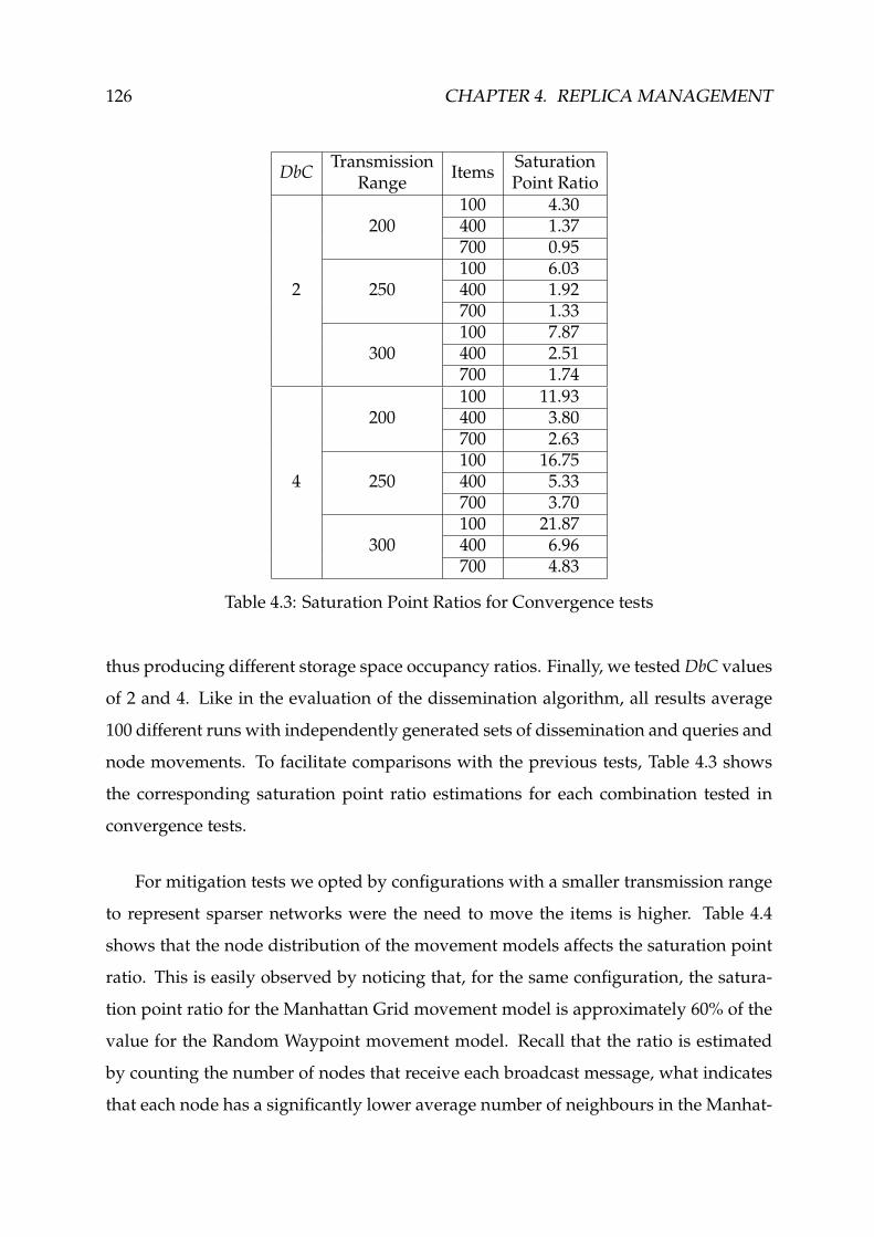
126 CHAPTER 4. REPLICA MANAGEMENT
DbCTransmission
ItemsSaturation
Range Point Ratio
2
200100 4.30400 1.37700 0.95
250100 6.03400 1.92700 1.33
300100 7.87400 2.51700 1.74
4
200100 11.93400 3.80700 2.63
250100 16.75400 5.33700 3.70
300100 21.87400 6.96700 4.83
Table 4.3: Saturation Point Ratios for Convergence tests
thus producing different storage space occupancy ratios. Finally, we testedDbC values
of 2 and 4. Like in the evaluation of the dissemination algorithm, all results average
100 different runs with independently generated sets of dissemination and queries and
node movements. To facilitate comparisons with the previous tests, Table 4.3 shows
the corresponding saturation point ratio estimations for each combination tested in
convergence tests.
For mitigation tests we opted by configurations with a smaller transmission range
to represent sparser networks were the need to move the items is higher. Table 4.4
shows that the node distribution of the movement models affects the saturation point
ratio. This is easily observed by noticing that, for the same configuration, the satura-
tion point ratio for the Manhattan Grid movement model is approximately 60% of the
value for the Random Waypoint movement model. Recall that the ratio is estimated
by counting the number of nodes that receive each broadcast message, what indicates
that each node has a significantly lower average number of neighbours in the Manhat-
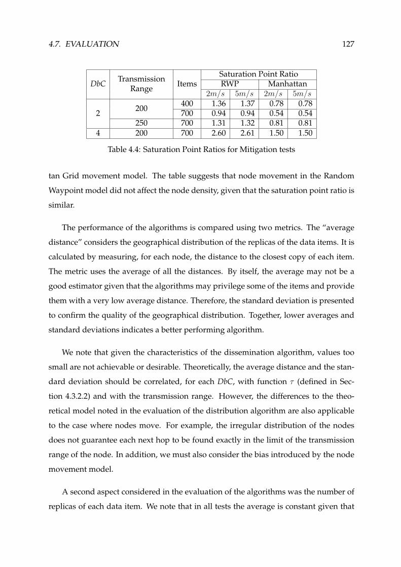
4.7. EVALUATION 127
DbCTransmissionRange
ItemsSaturation Point RatioRWP Manhattan
2m/s 5m/s 2m/s 5m/s
2200
400 1.36 1.37 0.78 0.78700 0.94 0.94 0.54 0.54
250 700 1.31 1.32 0.81 0.814 200 700 2.60 2.61 1.50 1.50
Table 4.4: Saturation Point Ratios for Mitigation tests
tan Grid movement model. The table suggests that node movement in the Random
Waypoint model did not affect the node density, given that the saturation point ratio is
similar.
The performance of the algorithms is compared using two metrics. The “average
distance” considers the geographical distribution of the replicas of the data items. It is
calculated by measuring, for each node, the distance to the closest copy of each item.
The metric uses the average of all the distances. By itself, the average may not be a
good estimator given that the algorithms may privilege some of the items and provide
them with a very low average distance. Therefore, the standard deviation is presented
to confirm the quality of the geographical distribution. Together, lower averages and
standard deviations indicates a better performing algorithm.
We note that given the characteristics of the dissemination algorithm, values too
small are not achievable or desirable. Theoretically, the average distance and the stan-
dard deviation should be correlated, for each DbC, with function τ (defined in Sec-
tion 4.3.2.2) and with the transmission range. However, the differences to the theo-
retical model noted in the evaluation of the distribution algorithm are also applicable
to the case where nodes move. For example, the irregular distribution of the nodes
does not guarantee each next hop to be found exactly in the limit of the transmission
range of the node. In addition, we must also consider the bias introduced by the node
movement model.
A second aspect considered in the evaluation of the algorithms was the number of
replicas of each data item. We note that in all tests the average is constant given that

128 CHAPTER 4. REPLICA MANAGEMENT
the storage space and the number of items is also constant. The metric used was the
standard deviation of the number of copies of each data item. The average is plotted to
allow a visual estimation of its proportion to the standard deviation. Again, the ideal
value of the standard deviation may not be zero. This is because the most adequate
number of replicas will depend of their location. For example, data items with replicas
stored at the nodes closer to the centre of the simulated space may require a smaller
number of replicas.
The evaluation compares the performance of the algorithms with each other and
with the state that was initially found after the dissemination phase. To observe the
evolution of the algorithms with time, snapshots of the state and location of the nodes
are taken at periodic intervals of each test. The first snapshot occurs at the end of the
dissemination phase. Plots represent this moment as time 0. The second snapshot
is taken 300s after, thus being coincident with the moment at which nodes stop in
convergence tests and queries start. A snapshot is taken again every 400s, with the last
one being coincident with the end of the simulation.
4.7.2.1 Probability of Insertion
The Probabilistic algorithm use two constants: prep dictates the probability of a trans-
mitting node to replace a record in the HERALDmessage; pins the probability of an item
being inserted when the node has some storage space entries marked with the replace
flag set to true. In this evaluation, we assume that prep should be necessarily small: if
records are frequently replaced, the TFS field is always kept at a low value. This would
prevent nodes more distant from receiving records with an high TFS and therefore,
from inserting the data items. In the simulations, we used a constant probability of 0.2
for prep as we considered that it represents a good tradeoff between the refreshment of
the records in the message and their continuation for being used in latter updates.
A definitive value for pins however is harder to establish. Intuitively, an higher
value of pins should provide a more aggressive update policy, that converges more
rapidly for the leveraging of the items distribution. However, if pins is excessively
4.7. EVALUATION 129
high, different neighbour nodes, receiving the same message will store the same item,
creating an undesirable level of redundancy for the item in some locations. Figure 4.25
compare the performance of two versions of the Probabilistic algorithm using pins = 0.5
and pins = 0.8 in the convergence tests.
Contrary to our expectations, the performance of the algorithms is very similar. In
some cases, pins = 0.8 presents an average smaller by a few meters in the earlier stages
of the tests. The difference tends to be attenuated later. In the Probabilistic algorithm,
a 30% difference in the probability may provide an almost negligible contribution to
the speed at which the algorithm improves the item distribution. Such a smaller differ-
ence suggests that a comparison of both variants with the remaining algorithms would
not provide a valuable contribution to the evaluation. Evaluation of convergence and
mitigation tests omit the results for pins = 0.5.
The following analysis will also omit results for 250 and 300m when DbC= 4. This
is justified by observing that in Figure 4.25 there is a small increase of the average
distance between the end of the dissemination phase (t = 0s) and the end of the move-
ment period (t = 300s). With DbC= 4, the distance between the replicas at the end of
the dissemination phase is close to what is achieved after the randommovement of the
nodes in a closed region with the predefined dimension.
4.7.2.2 Convergence Tests
The simulation results for the convergence tests are presented from Figure 4.26 to
Figure 4.29. The figures show that, in general, the four algorithms reduce the “average
distance” metric, in a tendency to correct the bad distribution that can be found after
nodes have moved. The standard deviation and the average curves exhibit a similar
pattern, suggesting that the leveraging is being equally distributed by the data items.
Not surprisingly, the Probabilistic algorithm is the algorithm that reacts faster to the
biased distribution. This is due to the number of data items that can be shuffled on
each query. Algorithms that keep the number of replicas constant will shuffle at most
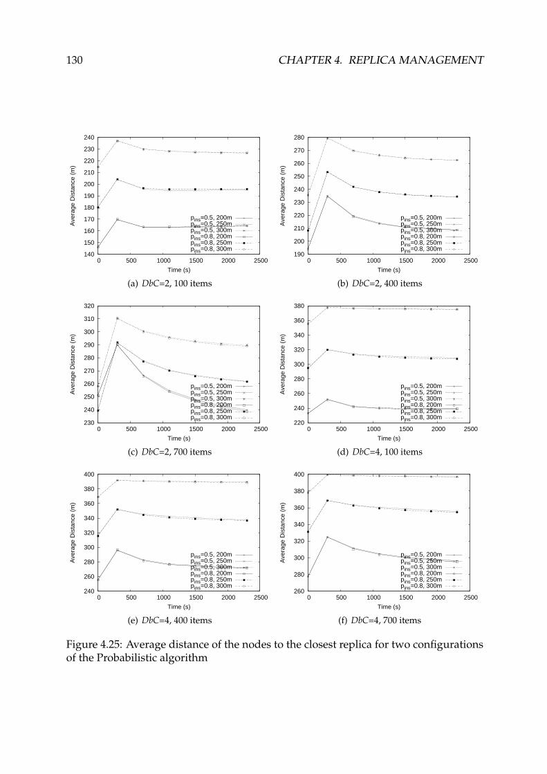
130 CHAPTER 4. REPLICA MANAGEMENT
140
150
160
170
180
190
200
210
220
230
240
0 500 1000 1500 2000 2500
Ave
rage
Dis
tanc
e (m
)
Time (s)
pins=0.5, 200mpins=0.5, 250mpins=0.5, 300mpins=0.8, 200mpins=0.8, 250mpins=0.8, 300m
(a) DbC=2, 100 items
190
200
210
220
230
240
250
260
270
280
0 500 1000 1500 2000 2500
Ave
rage
Dis
tanc
e (m
)
Time (s)
pins=0.5, 200mpins=0.5, 250mpins=0.5, 300mpins=0.8, 200mpins=0.8, 250mpins=0.8, 300m
(b) DbC=2, 400 items
230
240
250
260
270
280
290
300
310
320
0 500 1000 1500 2000 2500
Ave
rage
Dis
tanc
e (m
)
Time (s)
pins=0.5, 200mpins=0.5, 250mpins=0.5, 300mpins=0.8, 200mpins=0.8, 250mpins=0.8, 300m
(c) DbC=2, 700 items
220
240
260
280
300
320
340
360
380
0 500 1000 1500 2000 2500
Ave
rage
Dis
tanc
e (m
)
Time (s)
pins=0.5, 200mpins=0.5, 250mpins=0.5, 300mpins=0.8, 200mpins=0.8, 250mpins=0.8, 300m
(d) DbC=4, 100 items
240
260
280
300
320
340
360
380
400
0 500 1000 1500 2000 2500
Ave
rage
Dis
tanc
e (m
)
Time (s)
pins=0.5, 200mpins=0.5, 250mpins=0.5, 300mpins=0.8, 200mpins=0.8, 250mpins=0.8, 300m
(e) DbC=4, 400 items
260
280
300
320
340
360
380
400
0 500 1000 1500 2000 2500
Ave
rage
Dis
tanc
e (m
)
Time (s)
pins=0.5, 200mpins=0.5, 250mpins=0.5, 300mpins=0.8, 200mpins=0.8, 250mpins=0.8, 300m
(f) DbC=4, 700 items
Figure 4.25: Average distance of the nodes to the closest replica for two configurationsof the Probabilistic algorithm

4.7. EVALUATION 131
80
90
100
110
120
130
140
150
160
170
0 500 1000 1500 2000 2500
Dis
tanc
e (m
)
Time (s)
DefaultSwap On QueryAdvertise State
Probabilistic
(a) Distance, 100 items
1
1.5
2
2.5
3
3.5
4
4.5
5
5.5
0 500 1000 1500 2000 2500
Cop
ies
Time (s)
DefaultSwap On QueryAdvertise State
ProbabilisticAverage
(b) Copies, 100 items
120
140
160
180
200
220
240
0 500 1000 1500 2000 2500
Dis
tanc
e (m
)
Time (s)
(c) Distance, 400 items
1
1.5
2
2.5
3
3.5
0 500 1000 1500 2000 2500
Cop
ies
Time (s)
(d) Copies, 400 items
140
160
180
200
220
240
260
280
300
0 500 1000 1500 2000 2500
Dis
tanc
e (m
)
Time (s)
(e) Distance, 700 items
1
1.2
1.4
1.6
1.8
2
2.2
2.4
2.6
0 500 1000 1500 2000 2500
Cop
ies
Time (s)
(f) Copies, 700 items
Figure 4.26: Convergence tests when DbC=2 and transmission range=200m

132 CHAPTER 4. REPLICA MANAGEMENT
80
100
120
140
160
180
200
220
0 500 1000 1500 2000 2500
Dis
tanc
e (m
)
Time (s)
DefaultSwap On QueryAdvertise State
Probabilistic
(a) Distance, 100 items
0.5
1
1.5
2
2.5
3
3.5
4
0 500 1000 1500 2000 2500
Cop
ies
Time (s)
DefaultSwap On QueryAdvertise State
ProbabilisticAverage
(b) Copies, 100 items
100
120
140
160
180
200
220
240
260
0 500 1000 1500 2000 2500
Dis
tanc
e (m
)
Time (s)
(c) Distance, 400 items
0.8
1
1.2
1.4
1.6
1.8
2
2.2
2.4
2.6
2.8
3
0 500 1000 1500 2000 2500
Cop
ies
Time (s)
(d) Copies, 400 items
140
160
180
200
220
240
260
280
300
0 500 1000 1500 2000 2500
Dis
tanc
e (m
)
Time (s)
(e) Distance, 700 items
0.8
1
1.2
1.4
1.6
1.8
2
2.2
2.4
0 500 1000 1500 2000 2500
Cop
ies
Time (s)
(f) Copies, 700 items
Figure 4.27: Convergence tests when DbC=2 and transmission range=250m
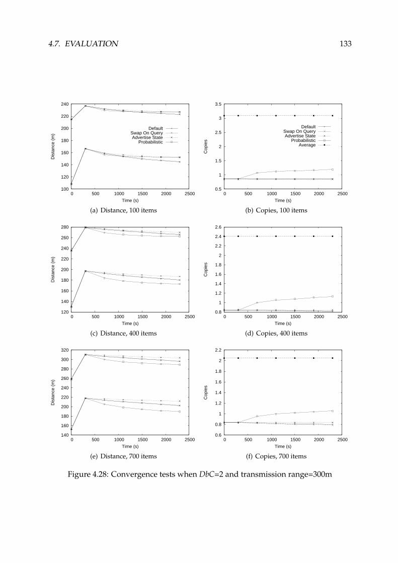
4.7. EVALUATION 133
100
120
140
160
180
200
220
240
0 500 1000 1500 2000 2500
Dis
tanc
e (m
)
Time (s)
DefaultSwap On QueryAdvertise State
Probabilistic
(a) Distance, 100 items
0.5
1
1.5
2
2.5
3
3.5
0 500 1000 1500 2000 2500
Cop
ies
Time (s)
DefaultSwap On QueryAdvertise State
ProbabilisticAverage
(b) Copies, 100 items
120
140
160
180
200
220
240
260
280
0 500 1000 1500 2000 2500
Dis
tanc
e (m
)
Time (s)
(c) Distance, 400 items
0.8
1
1.2
1.4
1.6
1.8
2
2.2
2.4
2.6
0 500 1000 1500 2000 2500
Cop
ies
Time (s)
(d) Copies, 400 items
140
160
180
200
220
240
260
280
300
320
0 500 1000 1500 2000 2500
Dis
tanc
e (m
)
Time (s)
(e) Distance, 700 items
0.6
0.8
1
1.2
1.4
1.6
1.8
2
2.2
0 500 1000 1500 2000 2500
Cop
ies
Time (s)
(f) Copies, 700 items
Figure 4.28: Convergence tests when DbC=2 and transmission range=300m

134 CHAPTER 4. REPLICA MANAGEMENT
120
140
160
180
200
220
240
260
0 500 1000 1500 2000 2500
Dis
tanc
e (m
)
Time (s)
DefaultSwap On QueryAdvertise State
Probabilistic
(a) Distance, 100 items
0.8
1
1.2
1.4
1.6
1.8
2
2.2
2.4
2.6
2.8
3
0 500 1000 1500 2000 2500
Cop
ies
Time (s)
DefaultSwap On QueryAdvertise State
ProbabilisticAverage
(b) Copies, 100 items
140
160
180
200
220
240
260
280
300
0 500 1000 1500 2000 2500
Dis
tanc
e (m
)
Time (s)
(c) Distance, 400 items
0.8
1
1.2
1.4
1.6
1.8
2
2.2
2.4
0 500 1000 1500 2000 2500
Cop
ies
Time (s)
(d) Copies, 400 items
160
180
200
220
240
260
280
300
320
340
0 500 1000 1500 2000 2500
Dis
tanc
e (m
)
Time (s)
(e) Distance, 700 items
0.6
0.8
1
1.2
1.4
1.6
1.8
2
0 500 1000 1500 2000 2500
Cop
ies
Time (s)
(f) Copies, 700 items
Figure 4.29: Convergence tests when DbC=4 and transmission range=200m

4.7. EVALUATION 135
two items. The default algorithm at most one while an undefined number of data items
can be shuffledwhen the Probabilistic algorithm is used. TheAdvertise State algorithm is
penalised by the frequent impossibility of swapping data items. As it can be observed,
the algorithm is particularly slower than the remaining when the average number of
copies is smaller. These are the cases where the probability of receiving a reply from
the producer of the item is higher.
In general, algorithms converge to some value between the average distance at
the end of the dissemination phase and at the end of the movement phase. That is,
although attenuating the impact of the node movement, the algorithms do not bring
the average distance to the low value that is achieved by the dissemination algorithm.
We attribute this behaviour to two interrelated factors.
1. The number of queries that may result in a shuffle of some data item decreases
with time. As a result of their operation, all algorithms progressively increase the
probability of finding a data item within the expected distance. Therefore, the
number of queries that will reach the conditions required by each algorithm for
shuffling is reduced. Not surprisingly, the “curve” that results from this effect is
more visible in the Probabilistic algorithm, the only one that can shuffle more than
one data item unrelated with the query.
2. Algorithms may be achieving a satisfactory distribution with a distance higher
than the one provided by the dissemination algorithm. This is expected given
that it was already shown that the dissemination algorithm induces excessive
redundancy. This claim is supported by noticing that the point to where the items
appear to converge is higher when the number of items is lower, that is, when
there is more space at the nodes for storing the redundant copies.
Results for the different algorithms are closer when there are less items adver-
tised. In particular, with 100 items, all algorithms presentmarginal differences between
them, with advantage for the algorithms that do not piggyback HERALD messages on

136 CHAPTER 4. REPLICA MANAGEMENT
queries. These algorithms tend to converge to an average distance lower than the re-
maining.
An observation of the graphics for the number of copies show that the algorithms
use different methods for achieving their goals. In particular, the Probabilistic algorithm
rapidly deteriorates the standard deviation of the number of copies while decreasing
the average distance. This indicates that the number of replicas of the items is less ho-
mogeneous in the Probabilistic algorithm. This can be attributed to i) a deviation of the
algorithm, if the preferred items are selected due to some possible random criteria; or
ii) an improvement of the geographical distribution that takes into account the location
of each replica. Results suggest that heterogeneity can be attributed to improvements
in the geographical distribution.
In general, the random algorithm presents the lowest average distance, even when
the standard deviation of the number of copies is significantly higher, what suggests
that the algorithm is improving the distribution. That is, the algorithm achieves a bet-
ter performance with a bigger deviation in the number of copies than the remaining,
which keep the number of copies close to what was determined during the dissemina-
tion. We interpret this result as a confirmation that the algorithm helps to remove the
additional redundancy that was already shown to be created by PADIS.
A particular case is observed in Figures 4.26(e) and 4.26(f), which is the only test
performed with a Saturation Point Ratio below 1. Recall that in this case, the algorithm
is unable to provide its properties given that the storage space made available by the
nodes is not sufficient for keeping the desired number of replicas. In this test, the Proba-
bilistic algorithm reduces the standard deviation of the number of copies, showing that
the grow that is visible in the remaining scenarios can be inverted in some cases. As a
result, the algorithm is able to improve the average distance to a value that is clearly
below the remaining and even below the one that was achieved by the dissemination
algorithm.

4.7. EVALUATION 137
200
250
300
350
400
450
0 500 1000 1500 2000 2500
Dis
tanc
e (m
)
Time (s)
DefaultSwap On QueryAdvertise State
ProbabilisticNo Queries
(a) Distance, RandomWaypoint
200
250
300
350
400
450
0 500 1000 1500 2000 2500
Dis
tanc
e (m
)
Time (s)
(b) Distance, Manhattan
0.6
0.8
1
1.2
1.4
1.6
1.8
2
2.2
2.4
0 500 1000 1500 2000 2500
Cop
ies
Time (s)
DefaultSwap On QueryAdvertise State
ProbabilisticAverage
(c) Copies, RandomWaypoint
0.6
0.8
1
1.2
1.4
1.6
1.8
2
2.2
2.4
0 500 1000 1500 2000 2500
Cop
ies
Time (s)
(d) Copies, Manhattan
Figure 4.30: Mitigation tests with 200m transmission range, 2m/s average speed, 700items and DbC=4
4.7.2.3 Mitigation Tests
In the mitigation tests, the shuffling algorithms were compared using the Random
Waypoint and the Manhattan Grid movement models. The simulation results are de-
picted from Figure 4.30 to Figure 4.37. The figures have been arranged by average
speed and from the highest to the lowest saturation point ratio. The plots showing the
metric distance of the nodes to the closest copy of each item also present the results for
control tests. In these tests nodes move but no queries are made. Given that in the re-
maining, shuffling always results from queries, the tests evidence what would happen
if no shuffling was used.
Recall from Table 4.4 that using the same configurations, the Manhattan Grid

138 CHAPTER 4. REPLICA MANAGEMENT
150
200
250
300
350
0 500 1000 1500 2000 2500
Dis
tanc
e (m
)
Time (s)
DefaultSwap On QueryAdvertise State
ProbabilisticNo Queries
(a) Distance, RandomWaypoint
150
200
250
300
350
0 500 1000 1500 2000 2500
Dis
tanc
e (m
)
Time (s)
(b) Distance, Manhattan
1
1.5
2
2.5
3
3.5
0 500 1000 1500 2000 2500
Cop
ies
Time (s)
DefaultSwap On QueryAdvertise State
ProbabilisticAverage
(c) Copies, RandomWaypoint
1
1.5
2
2.5
3
3.5
0 500 1000 1500 2000 2500
Cop
ies
Time (s)
(d) Copies, Manhattan
Figure 4.31: Mitigation tests with 200m transmission range, 2m/s average speed, 400items and DbC=2
movement model tests present a saturation point ratio that is approximately 60% of
the value for the Random Waypoint tests. The impact of the saturation point ratio is
clearly visible in side-by-side comparisons of both movement models.
The average distance of both movement models at the end of the dissemination
phase (in the plots corresponding to time 0s) and at the beginning of the query phase
(time 300s) present a similar pattern. At the end of the dissemination phase, and with
DbC=2, the Random Waypoint movement model presents an average distance that
is 55% ≈ 60% of the average distance exhibited by the Manhattan Grid movement
model. At the beginning of the query phase, the distributions become closer and are
in the interval 65% ≈ 69%. As expected, larger DbC’s also contribute to attenuate the

4.7. EVALUATION 139
150
200
250
300
350
400
0 500 1000 1500 2000 2500
Dis
tanc
e (m
)
Time (s)
DefaultSwap On QueryAdvertise State
ProbabilisticNo Queries
(a) Distance, RandomWaypoint
150
200
250
300
350
400
0 500 1000 1500 2000 2500
Dis
tanc
e (m
)
Time (s)
(b) Distance, Manhattan
0.8
1
1.2
1.4
1.6
1.8
2
2.2
2.4
2.6
0 500 1000 1500 2000 2500
Cop
ies
Time (s)
DefaultSwap On QueryAdvertise State
ProbabilisticAverage
(c) Copies, RandomWaypoint
0.8
1
1.2
1.4
1.6
1.8
2
2.2
2.4
2.6
0 500 1000 1500 2000 2500
Cop
ies
Time (s)
(d) Copies, Manhattan
Figure 4.32: Mitigation tests with 250m transmission range, 2m/s average speed, 700items and DbC=2
differences between the movement models and the ratios become around 65% and 70%
respectively at times 0s and 300s.
A common trend that can be found in the Random Waypoint model tests is the
stabilisation of the average distance, aligned with the control tests. This suggests that
the shuffling algorithms are unable to keep the pace with the changes in the topology.
These difficulties are more evident when we compare the graphics for the different
speeds with the graphics presented for the same configuration in convergence tests. It
can be observed that the tests for nodes moving at 5m/s are those presenting the lowest
gains and that convergence tests always present the highest gains. However, we note
that the requirement that nodes never stop is particularly demanding. As convergence

140 CHAPTER 4. REPLICA MANAGEMENT
200
250
300
350
400
0 500 1000 1500 2000 2500
Dis
tanc
e (m
)
Time (s)
DefaultSwap On QueryAdvertise State
ProbabilisticNo Queries
(a) Distance, RandomWaypoint
200
250
300
350
400
0 500 1000 1500 2000 2500
Dis
tanc
e (m
)
Time (s)
(b) Distance, Manhattan
0.8
1
1.2
1.4
1.6
1.8
2
2.2
2.4
2.6
0 500 1000 1500 2000 2500
Cop
ies
Time (s)
DefaultSwap On QueryAdvertise State
ProbabilisticAverage
(c) Copies, RandomWaypoint
0.8
1
1.2
1.4
1.6
1.8
2
2.2
2.4
2.6
0 500 1000 1500 2000 2500
Cop
ies
Time (s)
(d) Copies, Manhattan
Figure 4.33: Mitigation tests with 200m transmission range, 2m/s average speed, 700items and DbC=2
tests have shown, soon after the topology has stabilised, the algorithms are able to
improve the average distance. In a real scenario, we expect the algorithms to present
a behaviour that would be between the two extreme situations. We note also that
the pace of queries in these tests is constant. If the number of queries was increased,
the number of opportunities for the algorithms to improve the shuffling would also
increase and we should expect better results.
The Probabilistic algorithm is the one whose results tend to differentiate more from
the remaining. In some cases, it is even presenting results that are worst than those
observed in the control tests, suggesting that the algorithm is making more harm than
good to the distribution. This is consistent with the behaviour observed in the conver-

4.7. EVALUATION 141
200
250
300
350
400
450
0 500 1000 1500 2000 2500
Dis
tanc
e (m
)
Time (s)
DefaultSwap On QueryAdvertise State
ProbabilisticNo Queries
(a) Distance, RandomWaypoint
200
250
300
350
400
450
0 500 1000 1500 2000 2500
Dis
tanc
e (m
)
Time (s)
(b) Distance, Manhattan
0.6
0.8
1
1.2
1.4
1.6
1.8
2
2.2
2.4
0 500 1000 1500 2000 2500
Cop
ies
Time (s)
DefaultSwap On QueryAdvertise State
ProbabilisticAverage
(c) Copies, RandomWaypoint
0.6
0.8
1
1.2
1.4
1.6
1.8
2
2.2
2.4
0 500 1000 1500 2000 2500
Cop
ies
Time (s)
(d) Copies, Manhattan
Figure 4.34: Mitigation tests with 200m transmission range, 5m/s average speed, 700items and DbC=4
gence tests where it was noticed that the algorithm tends to stabilise at some average
distance above the minimum, specially when the saturation point ratio is high. We
note that like before, Figure 4.33 shows that in the lowest saturation point ratio we ex-
perimented, the Probabilistic algorithm is again providing the lowest average distance,
although not so clearly distinguishable from the remaining algorithms.
The results for the Manhattan Grid movement model on the other hand contra-
dict the previous analysis by showing that even when nodes move it is still possible
to improve the average distance metric. The behaviour of each algorithm concerning
the average distance is comparable with the graphics presented for convergence tests.
We emphasise two aspects that are likely to justify these differences: i) the substan-

142 CHAPTER 4. REPLICA MANAGEMENT
150
200
250
300
350
0 500 1000 1500 2000 2500
Dis
tanc
e (m
)
Time (s)
DefaultSwap On QueryAdvertise State
ProbabilisticNo Queries
(a) Distance, RandomWaypoint
150
200
250
300
350
0 500 1000 1500 2000 2500
Dis
tanc
e (m
)
Time (s)
(b) Distance, Manhattan
1
1.5
2
2.5
3
3.5
0 500 1000 1500 2000 2500
Cop
ies
Time (s)
DefaultSwap On QueryAdvertise State
ProbabilisticAverage
(c) Copies, RandomWaypoint
1
1.5
2
2.5
3
3.5
0 500 1000 1500 2000 2500
Cop
ies
Time (s)
(d) Copies, Manhattan
Figure 4.35: Mitigation tests with 200m transmission range, 5m/s average speed, 400items and DbC=2
tially smaller number of neighbours and corresponding saturation point ratio; and ii)
the highest average distance at the end of the dissemination phase, even with satura-
tion point ratios above one (see for example, the results for this movement model in
Figures 4.30 and 4.34 which have a saturation point ratio of 1.5).
In these tests, the Probabilistic algorithm clearly outperforms the remaining. The
algorithm rapidly makes the average distance converge to a value that is, in general,
below the achieved with the initial dissemination. It should also be noted that, con-
tradicting the rule observed in the majority of the convergence tests, the standard de-
viation of the number of copies also tends to decrease. This confirms that none of the
algorithms applies a particular bias to the number of copies of some item that could,

4.7. EVALUATION 143
150
200
250
300
350
400
0 500 1000 1500 2000 2500
Dis
tanc
e (m
)
Time (s)
DefaultSwap On QueryAdvertise State
ProbabilisticNo Queries
(a) Distance, RandomWaypoint
150
200
250
300
350
400
0 500 1000 1500 2000 2500
Dis
tanc
e (m
)
Time (s)
(b) Distance, Manhattan
0.8
1
1.2
1.4
1.6
1.8
2
2.2
2.4
2.6
0 500 1000 1500 2000 2500
Cop
ies
Time (s)
DefaultSwap On QueryAdvertise State
ProbabilisticAverage
(c) Copies, RandomWaypoint
0.8
1
1.2
1.4
1.6
1.8
2
2.2
2.4
2.6
0 500 1000 1500 2000 2500
Cop
ies
Time (s)
(d) Copies, Manhattan
Figure 4.36: Mitigation tests with 250m transmission range, 5m/s average speed, 700items and DbC=2
in the long term, affect the distribution. In fact, the standard deviation adapts to the
networking environment and can either increase or decrease to improve the average
distance.
The Advertise State algorithm is the one that exhibits the worst performance. In the
Manhattan Grid tests it is in general coincident with the control tests. We attribute
this behaviour to two particular features of the algorithm: i) its strong commitment
on the preservation of the number of replicas and ii) an incorrect application of the
replace flag that results from node movement. Recall from Section 4.5.3 that this algo-
rithm only advertises items stored with the replace flag set to false, meaning that no
other replica is known to be in the neighbourhood. However, in the presence of node

144 CHAPTER 4. REPLICA MANAGEMENT
150
200
250
300
350
400
0 500 1000 1500 2000 2500
Dis
tanc
e (m
)
Time (s)
DefaultSwap On QueryAdvertise State
ProbabilisticNo Queries
(a) Distance, RandomWaypoint
150
200
250
300
350
400
0 500 1000 1500 2000 2500
Dis
tanc
e (m
)
Time (s)
(b) Distance, Manhattan
1
1.2
1.4
1.6
1.8
2
2.2
2.4
2.6
0 500 1000 1500 2000 2500
Cop
ies
Time (s)
DefaultSwap On QueryAdvertise State
ProbabilisticAverage
(c) Copies, RandomWaypoint
1
1.2
1.4
1.6
1.8
2
2.2
2.4
2.6
0 500 1000 1500 2000 2500
Cop
ies
Time (s)
(d) Copies, Manhattan
Figure 4.37: Mitigation tests with 200m transmission range, 5m/s average speed, 700items and DbC=2
movement, nodes establish temporarily contact with others which also store replicas
of the same items. Due to the lack of refreshment of the flag, after some time, nodes
will cease to advertise their items, rendering the algorithm useless. The definition of
an adequate refreshment criteria for the flag will always depend of specific conditions
of the environment where the algorithm is going to be applied, removing generality to
the algorithm.
These results confirm the trend that emerged from the analysis of the convergence
tests. Shuffling algorithms can contribute to improve the distribution performed by the
dissemination algorithm, specially in the cases where the saturation point ratio is very
low. However, we note that in the general case, PADIS gives a valuable contribution to

4.8. SUMMARY 145
the overall performance of the framework. In particular, it provides an estimate of the
number of copies that are required and places them in adequate locations. Shuffling
algorithms help by refining the dissemination. However, they depend of the queries
and may suffer performance problems in some movement patterns.
4.8 Summary
This chapter presented PADIS, an algorithm for disseminating information in ad-
hoc networks. The algorithm is fully distributed as it does not assume the presence
of only a few data sources in the ad-hoc network; each node, instead, is expected to
advertise its own data items. The main goal of the algorithm is to ensure an even
geographical distribution of the disseminated data items, so that requests for a given
data item are satisfied by some nodes close to the source of the query. Data items are
disseminated with a counter to provide a minimal distance between the copies. The
use of Pampa reduces the number of messages required for propagation and increases
the geographical distance between the hops.
The chapter also presented a complement to PADIS, that consists on different al-
gorithms for leveraging item distribution in the presence of node movement. The four
algorithms described use different techniques and put different efforts in the preser-
vation of the number of replicas. The algorithms require a limited amount of power,
given that they either use point-to-point messages or piggyback their information in
messages used for data retrieval.
Simulation results show that PADIS achieves a fair dissemination of items through-
out the network although the results are slightly worst thanwhat could be theoretically
expected. The results are justified by the impossibility of providing an ideal network-
ing environment.
Comparative simulations of the shuffling algorithms have confirmed their capa-
bility to improve data distribution, particularly in the less favourable conditions for

146 CHAPTER 4. REPLICA MANAGEMENT
PADIS. The Probabilistic shuffling algorithm clearly stands, by lowering the average
distance from each node to each data item faster than the remaining.

5Application
It is easy to find in the literature different applications for data distribution algo-
rithms in mobile ad hoc networks. Good examples are the support of cooperative
work performed by geological teams during their field studies (Hara, 2001) or the dis-
tributed caching of web pages (Sailhan & Issarny, 2003). In general, applications can
be arranged in two classes: those that provide innovative services that emerge from
the possibilities offered by the mobility of the devices and those that aim to extend the
different services typically provided by the Internet to the ad hoc networking environ-
ment. This chapter focus on the later.
Many of the services provided in the Internet are implemented using a client-server
model requiring well known and reliable servers. In MANETs, a comparable model
can only be achieved by replicating the service in multiple nodes. Therefore, a chal-
lenge that is posed in extending Internet applications to MANETs is to devise alter-
native implementations that are able to cope with the constraints of the networking
environment. Ideally, the alternatives should be able to mask the differences of the un-
derlying environment so that applications developed for the wired setting could run
transparently in MANETs.
This chapter shows how the algorithms described in this thesis have been applied
to support the Session Initiation Protocol (SIP) (Rosenberg et al., 2002) in ad hoc net-
works. The SIP architecture is network-centric (Schulzrinne & Rosenberg, 2000), as
SIP relies on network entities to assist end users in their operations. SIP deployment
in server-less environments, such as MANETs, is thus not straightforward. For self-
containment, the chapter begins by providing in Section 5.1 a short overview of SIP and
147
148 CHAPTER 5. APPLICATION
decentralised SIP (dSIP) (Leggio et al., 2005), a solution for deploying SIP in MANETs.
dSIP was initially proposed in the context of 1 hopMANETs: those where all nodes
are in the transmission range of each other. In addition, dSIP exhibited scalability
problems. Section 5.2 describes SIPCache, a combination of PADIS with dSIP and with
a data gathering module, developed to mitigate dSIP’s previous limitations.
Section 5.3 evaluates the data gathering module of SIPCache. The chapter is con-
cluded with a summary of the results in Section 5.4.
5.1 Overview of SIP
The Session Initiation Protocol (SIP) (Rosenberg et al., 2002) is a signalling proto-
col designed by the IETF to initiate and manage multimedia communication sessions
in the Internet. A signalling protocol negotiates all the parameters necessary for a
communication session, e.g., its type (VoIP call, video call, chat) and characteristics
(e.g, audio codecs) used. A most relevant characteristic of SIP is its flexibility: SIP can
transparently signal any type of media session and is easily extendable to support new
features.
A SIP network is composed of multiple domains, each independently administered
by some organisation. Each domain provides a Registrar Server and a Proxy Server. In
order to use SIP services, it is necessary to register a user’s own contact information
in a SIP domain. Usually, the information consists in the SIP address, that is, the SIP
unique user name, also referred to as Address of Records (AOR), and the current IP
address. An association between a user’s AOR and his contact IP address is called a
“binding” and is stored in the Registrar Server for the domain. Queries are addressed
to Proxy Servers, who forwards them to the Registrar Server if the query is addressed to
some AOR of the local domain. Queries for AORs of other domains are forwarded to
the corresponding Proxy Server.
Authorised users communicate their bindings to the registrar server using a SIP

5.1. OVERVIEW OF SIP 149
Bob’s ProxyAlice’s ProxyAlice’s UA Bob’s UABob’s Registrar
INVITE (M1)
INVITE (M2)
REGISTER (R1)
200 OK (R2)
INVITE (M3)
Bob’s IP?
IP of Bob
Figure 5.1: Simplified logical message flow in SIP
REGISTER message. Figure 5.1 shows that Bob has registered to his registrar server
(message R1) and that the server has acknowledged the registration (message R2).
In general, when contacting a SIP user, a SIP client only knows the AOR of the
person to contact. Similarly to what happens in e-mail systems, the contact IP address
is typically unknown. In the example of Figure 5.1, user Alice, whowants to begin a SIP
session with Bob, sends an INVITE message first to the SIP Proxy Server of her domain
(message M1). The role of the proxy server is to locate, on behalf of the authorised
users, the final recipient of a SIP request. Alice’s proxy, thus, contacts the proxy serving
Bob’s domain (message M2).
Bob’s proxy recognises that the INVITE request is addressed to a user belonging
to its domain and exploits the location service, querying the domain registrar about
the contact address of the target user, as indicated by the dashed line messages in
Figure 5.1. The registrar returns to the proxy the contact information, and the message
is forwarded to destination (message M3). The location service related messages are
depicted using dashed lines to signal that the distinction between proxy and registrar
is merely logical: it is not uncommon that operators co-locate their functionalities into
the same host. The IETF has not defined a standard protocol for exploiting the location
service.

150 CHAPTER 5. APPLICATION
New SIPApplication
Standard SIPApplication
IP
Proximity Extensions Proximity Extensions
Proximity ManagerApplication
EnhancedAPI
SIP API
User Agent Server
Cache
Figure 5.2: Software architecture for decentralised SIP
5.1.1 Decentralised SIP
Mobile Ad hoc Networks are by definition self-managed networks without the
support of an underlying infrastructure composed for example of SIP proxies or reg-
istrar servers, fundamental to the correct behaviour of the SIP protocol. Decentralised
SIP (dSIP) (Leggio et al., 2005) is an architecture that overcomes this limitation, al-
lowing the use of SIP also in server-less environments, such as MANETs. In addi-
tion, dSIP extends standard SIP features with proximity functionalities for discovering
which users are present in the MANET.
The key idea of dSIP is to embed in each enabled device a basic subset of SIP
proxy and registrar server functionalities, so that dSIP devices are self-capable to main-
tain and exploit the location service. Decentralised SIP is particularly suited for small
MANETs, with few dozens of nodes at most.
The software architecture of dSIP is shown in Figure 5.2: the modules bordered
with solid lines are standard SIP modules in a device. The dashed modules are the
extensions defined by dSIP. In a standard SIP client, only the user agent (UA) side
of the stack would be present. In dSIP, the server module is added, and the server
standard capabilities are enhanced with the proximity functionalities. The interested
reader is referred to (Leggio et al., 2005) for a complete description of the role of each
module.
dSIP does not require the modification of the existing software modules of SIP

5.1. OVERVIEW OF SIP 151
INVITE (M1)
INVITE (M2)
Bob’s IP?
IP of Bob
REGISTER (R2)
200 OK (R3)
Alice’s UA User’s UA User’s UA Bob’s UA
REGISTER (R1)
200 OK (R3)
200 OK (R3)
Figure 5.3: Simplified logical message flow in dSIP
clients. Extensions are enabled by adding new submodules. This choice allows inter-
operability of dSIP UAs with standard SIP clients: a standard SIP application can be
deployed on top of dSIP equally well as an application that exploits dSIP proximity
functionalities. A native SIP application is unaware of the presence of a modified SIP
stack in the device, since it only utilises the standard SIP features. Moreover, a native
application can be utilised in MANETs, since the underlying middleware is able to
handle all the SIP messages sent by the application in the proper way.
The working principle of dSIP is that the user agent registers with the co-located
registrar server, according to standard SIP procedures, by sending internally a REGIS-
TER message. The server then registers the SIP user to the network spreading a SIP
REGISTER message. The server modules in the network receive the REGISTER mes-
sage, update their cache entry with the binding, and may reply to the registering node
by sending a “200 OK” confirmation message. The registering node server module
updates its cache with the bindings received from the other nodes. With this proce-
dure, also referred to as general registration, the SIP location service is maintained in
a distributed way among all the nodes. Figure 5.3 illustrates dSIP’s handling of SIP
REGISTER and INVITE messages.
A native SIP application sends a REGISTER message to its predefined registrar
server. The dSIP modules transparently intercepts the message and routes it to the
local server, ensuring interoperability with standard SIP applications.
152 CHAPTER 5. APPLICATION
Inviting a peer to a SIP session is similar: the INVITE message is routed to the
co-located server, which checks in its cache for a binding for the queried user. The IN-
VITE message is forwarded to the correct address if a match is found. dSIP proximity
functionalities extend SIP’s standard services by supporting queries for the list of users
in the network. This allows the user to begin sessions also with previously unknown
users.
5.2 SIPCache
dSIP works well in small networks. The design of dSIP assumes that all the server
module instances know the bindings of all users, what is not scalable. Moreover, dSIP
makes no assumption about the mechanism used for the spreading of the bindings.
dSIP was combined with PADIS to address these issues. The key idea of the result-
ing framework, named SIPCache, is to perform a partial replication of the AORs. The
architecture of SIPCache is depicted in Figure 5.4. SIPCache benefits of the geograph-
ical distribution of the replicas provided by PADIS to keep a copy of the AORs in the
proximity of any node. PADIS uses the original dSIP’s cache as its storage space. To
fully encompass the original dSIP facilities, SIPCache includes a data gathering mod-
ule supporting the proximity functionalities.
5.2.1 Dissemination and Retrieval Using PADIS
In SIPCache, the dissemination and retrieval algorithms described in Chapter 4 are
used to perform respectively the dissemination and query of bindings. The integration
of PADIS with dSIP required some minimal changes. For example, data items were
complemented with an expire field and a version number to allow nodes to purge old
records and keep track of the most up-to-date binding.
Figure 5.5 shows the logical flow of the dissemination in SIPCache. In comparison
with dSIP, it can be observed that the message flow reflects the PADIS data distribution
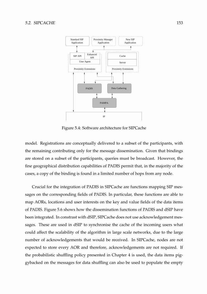
5.2. SIPCACHE 153
New SIPApplication
Standard SIPApplication
IP
User Agent
Proximity ManagerApplication
Cache
Server
Proximity Extensions Proximity Extensions
SIP APIEnhanced
API
PAMPA
PADIS Data Gathering
Figure 5.4: Software architecture for SIPCache
model. Registrations are conceptually delivered to a subset of the participants, with
the remaining contributing only for the message dissemination. Given that bindings
are stored on a subset of the participants, queries must be broadcast. However, the
fine geographical distribution capabilities of PADIS permit that, in the majority of the
cases, a copy of the binding is found in a limited number of hops from any node.
Crucial for the integration of PADIS in SIPCache are functions mapping SIP mes-
sages on the corresponding fields of PADIS. In particular, these functions are able to
map AORs, locations and user interests on the key and value fields of the data items
of PADIS. Figure 5.6 shows how the dissemination functions of PADIS and dSIP have
been integrated. In constrast with dSIP, SIPCache does not use acknowledgement mes-
sages. These are used in dSIP to synchronise the cache of the incoming users what
could affect the scalability of the algorithm in large scale networks, due to the large
number of acknowledgements that would be received. In SIPCache, nodes are not
expected to store every AOR and therefore, acknowledgements are not required. If
the probabilistic shuffling policy presented in Chapter 4 is used, the data items pig-
gybacked on the messages for data shuffling can also be used to populate the empty

154 CHAPTER 5. APPLICATION
INVITE (M2)
Bob’s IP?
IP of Bob
REGISTER (R2)
User’s UA Bob’s UA
REGISTER (R1)
User’s UA
INVITE (M1)
Alice’s UA User’s UA
Figure 5.5: Simplified logical message flow in SIPCache
1: procedure BINDING(SIPMessage)2: binding← EXTRACTBINDING(SIPMessage)3: PADIS.REGISTER(binding)4: end procedure
Figure 5.6: Binding dissemination in SIPCache
storage spaces of the new nodes.
Depending of the type of query performed, SIPCache may use either the data re-
trieval algorithm described in Chapter 4 if the query is aimed to a specific AOR (tar-
geted queries) or the data gathering module, described below, if the goal is to retrieve
a set of AORs matching some criteria. The pseudo-code for query handling is outlined
in Figure 5.7. The figure uses an abstract monitor for representing the suspension of
the thread of execution until a reply is found. In the case of targeted queries, the key is
passed to PADIS’s query method who will search the local cache and trigger one run
of the query algorithm if the reply is not locally available.
5.2.2 Data Gathering Module
One of the facilities provided by dSIP was to allow an user to retrieve a list of the
participants whose AOR satisfied some criteria. For example, users may find interest-
ing to learn about all available printers or to find other users in the ad hoc network
matching a specified profile. A query for all the people interested, e.g., in sports, can
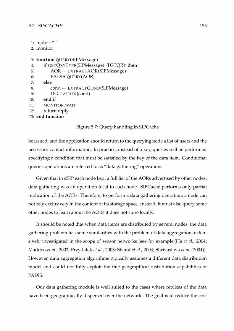
5.2. SIPCACHE 155
1: reply←” “2: monitor
3: function QUERY(SIPMessage)4: if GETQRYTYPE(SIPMessage)=TGTQRY then5: AOR← EXTRACTAOR(SIPMessage)6: PADIS.QUERY(AOR)7: else8: cond← EXTRACTCOND(SIPMessage)9: DG.GATHER(cond)10: end if11: MONITOR.WAIT12: return reply13: end function
Figure 5.7: Query handling in SIPCache
be issued, and the application should return to the querying node a list of users and the
necessary contact information. In practice, instead of a key, queries will be performed
specifying a condition that must be satisfied by the key of the data item. Conditional
queries operations are referred to as “data gathering” operations.
Given that in dSIP each node kept a full list of the AORs advertised by other nodes,
data gathering was an operation local to each node. SIPCache performs only partial
replication of the AORs. Therefore, to perform a data gathering operation, a node can
not rely exclusively in the content of its storage space. Instead, it must also query some
other nodes to learn about the AORs it does not store locally.
It should be noted that when data items are distributed by several nodes, the data
gathering problem has some similarities with the problem of data aggregation, exten-
sively investigated in the scope of sensor networks (see for example (He et al., 2004;
Madden et al., 2002; Przydatek et al., 2003; Sharaf et al., 2004; Shrivastava et al., 2004)).
However, data aggregation algorithms typically assumes a different data distribution
model and could not fully exploit the fine geographical distribution capabilities of
PADIS.
Our data gathering module is well suited to the cases where replicas of the data
have been geographically dispersed over the network. The goal is to reduce the cost

156 CHAPTER 5. APPLICATION
of each operation by limiting the search to the nodes located a few hops away from
the source, benefiting of the Pampa message dissemination capabilities. Data gather-
ing operations run in two phases: query dissemination and data delivery. In the first
phase, queries are disseminated within a bounded number of hops using Pampa. In
the data delivery phase, each node replies to the source of the first transmission of the
query it has received. Nodes that receive multiple replies are responsible for removing
redundancy of the data items they collect and to forward the aggregate to the source
of the query. A detailed description of the module is presented below.
5.2.2.1 Detailed Description
In a process similar to the one used by PADIS, each data gathering operation par-
titions the nodes in the network in clusters. The partitioning is triggered by the broad-
cast of a data GATHERING message using Pampa. Nodes selected for retransmitting
the message become cluster heads. A node becomes a member of at most two clusters:
of the one it leads (if any) and of the cluster headed by the node that transmitted the
first copy of the message it has received.
The main characteristic of our clustering approach is that it is stateless and
message-driven, that is, clusters are formed based only on the propagation of received
messages, as dictated by Pampa. There is no need to implement a dedicated member-
ship protocol, or for the cluster heads to keep state information on the nodes belonging
to their cluster. Each cluster head is responsible for preventing the delivery of redun-
dant data items to the source node by locally aggregating replies from the remaining
cluster members. An example of a cluster partitioning of a network is depicted in
Figure 5.8.
The use of Pampa gives a significant contribution to the performance and adapt-
ability of the data gathering module. As emphasised in Chapter 3, in the absence
of abnormal propagation effects, Pampa selects for retransmission the nodes that are
more distant from the previous source. Therefore, and using the same assumptions,
the module selects for cluster heads the nodes that are more distant from the sources

5.2. SIPCACHE 157
S
Cluster Head
H
H
H
H
H
H
Reply
Route
Figure 5.8: Propagation of gathering messages and replies
of the previous transmissions. The advantages of this approach are:
• a geographical extension of the coverage of each retransmission, allowing to re-
duce the diameter (in hops) of the query;
• an increase in the number of nodes on each cluster, allowing to collect more infor-
mation on each cluster head. Because more nodes are reached, the probabilities
of collecting all data items satisfying the condition also increases;
• a simple adaptation to different network conditions, as it was shown in the eval-
uation of Pampa.
As shown in Figure 5.9, a data gathering operation is triggered by the broadcast of
a GATHERING message using Pampa and containing the condition to be satisfied by
the data items. The message accumulates the path to be followed by the replies in a
routeStack field.
Each data gathering operation is performed using a ring search. The radius of the
ring is defined at the source of the query in a field commonly identified as Time-To-
Live (TTL), decremented by each node that forwards the message.
To limit the number of redundant replies, the message is filled up with data items
up to a maximum message size. These data items are selected from those that are
known to satisfy the condition and have been received in a previous transmission of
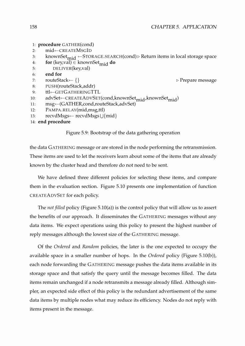
158 CHAPTER 5. APPLICATION
1: procedure GATHER(cond)2: mid←CREATEMSGID3: knownSetmid ←STORAGE.SEARCH(cond) ⊲ Return items in local storage space4: for (key,val) ∈ knownSetmid do5: DELIVER(key,val)6: end for7: routeStack← {} ⊲ Prepare message8: PUSH(routeStack,addr)9: ttl←GETGATHERINGTTL10: advSet←CREATEADVSET(cond,knownSetmid,knownSetmid)11: msg←(GATHER,cond,routeStack,advSet)12: PAMPA.RELAY(mid,msg,ttl)13: recvdMsgs← recvdMsgs
⋃
{mid}14: end procedure
Figure 5.9: Bootstrap of the data gathering operation
the data GATHERINGmessage or are stored in the node performing the retransmission.
These items are used to let the receivers learn about some of the items that are already
known by the cluster head and therefore do not need to be sent.
We have defined three different policies for selecting these items, and compare
them in the evaluation section. Figure 5.10 presents one implementation of function
CREATEADVSET for each policy.
The not filled policy (Figure 5.10(a)) is the control policy that will allow us to assert
the benefits of our approach. It disseminates the GATHERING messages without any
data items. We expect operations using this policy to present the highest number of
reply messages although the lowest size of the GATHERING message.
Of the Ordered and Random policies, the later is the one expected to occupy the
available space in a smaller number of hops. In the Ordered policy (Figure 5.10(b)),
each node forwarding the GATHERING message pushes the data items available in its
storage space and that satisfy the query until the message becomes filled. The data
items remain unchanged if a node retransmits a message already filled. Although sim-
pler, an expected side effect of this policy is the redundant advertisement of the same
data items by multiple nodes what may reduce its efficiency. Nodes do not reply with
items present in the message.

5.2. SIPCACHE 159
1: procedure CREATEADVSET(cond,firstSet,recvdSet)2: return {}3: end procedure
(a) Not filled
1: procedure CREATEADVSET(cond,firstSet,recvdSet)2: set← firstSet3: localSet← STORAGE.SEARCH(cond)4: while ¬FULL(set) do5: set← set
⋃
{x : x ∈ localSet ∧ x 6∈ set}6: end while7: return set8: end procedure
(b) Ordered
1: procedure CREATEADVSET(cond,firstSet,recvdSet)2: set← {}3: localSet← STORAGE.SEARCH(cond)4: bigSet← firstSet
⋃
recvdSet⋃
localSet5: while ¬FULL(set) do6: set← set
⋃
{x : x ∈ bigSet ∧ x 6∈ set}7: end while8: return set9: end procedure
(c) Random
Figure 5.10: Policies for filling data gathering messages with known data items
In the Random policy depicted in Figure 5.10(c), nodes snoop the network and col-
lect in a recvdSet set all the data items advertised in every retransmission they listen
of the GATHERING message. The items advertised are randomly selected from this set
and from those locally known by the node. The reply will not include any item that is
present in the recvdSet set. We expect this to be the most efficient redundancy removal
mechanism as it prevents the retransmission of data items known by several cluster
heads.
It should be noted that the selection of a policy does not imply a change in the
number of retransmissions of the GATHERING message, although it should affect the
number of bytes transmitted. The gains are expected to occur in the reduction of the

160 CHAPTER 5. APPLICATION
number of reply messages. We notice that the transmission of a frame implies both a
variable energy cost that depends of the number of bytes transmitted but also a fixed
cost (Feeney & Nilsson, 2001). In the fixed cost, one must account for example with
the collision avoidance protocol (which requires 3 link layer frames in IEEE802.11) as
well as the fixed sized headers of the lower level protocols. Therefore, policies that
require the transmission of more bytes may still provide non negligible energy savings
resulting from the transmission of a smaller number of messages.
Figure 5.11 shows the handling of a GATHERING message by the nodes. The prop-
agation strictly follows Pampa, which decides both the hold period and to forward or
not the message. The message will be replied if at the end of the hold period, Pampa
decides not to retransmit. A special case occurs when the dissemination phase is con-
cluded (signalled by the TTL field), in which the reply is immediately forwarded to the
cluster head.
If a node decides to retransmit, it decrements the TTL field of the message, updates
the data items to be forwarded according to the predefined policy and push its address
in the route stack, electing himself as cluster head. After retransmitting the message,
the node enters a second hold period defined by multiplying the value of the TTL field
by a constant. The value should be enough to permit the dissemination phase to be
concluded so that all replies can be successively collected by the cluster heads and
delivered to it before his timer expires.
Independently of being or not a cluster head, all nodes send a reply message only
when it is not empty. Figure 5.12 shows the pseudo-code of the reply phase of the data
gathering operation.
If a node receives a reply then it is either a cluster head or the source of the gather-
ing operation. Cluster heads collect all data items received in replies. The aggregate of
the replied data items, without duplicates, is forwarded to the previous cluster head.
A message may be delivered to a cluster head after its timer has expired. Nodes
do not keep any state about past operations. Therefore, when a node receives a reply

5.2. SIPCACHE 161
15: upon event PAMPA.RECEIVED(mid,(GATHER,cond,routeStack,advSet),ttl,holdTime)do
16: ifmid 6∈ recvdMsgs then17: recvdMsgs← recvdMsgs
⋃
{mid}18: knownSetmid ← advSet19: replySetmid ← {}20: ttlmid ← ttl− 121: if ttlmid > 0 then22: TIMER.SETALARM(holdTime,(FWD,mid))23: else24: PAMPA.DROP(mid)25: SENDREPLY(mid)26: end if27: else28: knownSetmid ← knownSetmid
⋃
advSet29: end if30: end upon
31: upon event TIMER.ALARM((FWD,mid)) do32: if PAMPA.DECIDE(mid) then33: FWDDG(mid)34: TIMER.SETALARM(kTime× ttlmid,(RPLY,mid))35: else36: PAMPA.DROP(mid)37: SENDREPLY(mid)38: end if39: end upon
Figure 5.11: Data Gathering message dissemination
for an unknown data gathering operation, it uses the route stack field to immediately
forward the message. Note that since the node does not keep any state, it can not re-
move redundant replies from the message. Redundancy could possibly be removed at
the next cluster head (if any) if it is delivered before its timer expires. In the worst case,
it is delivered to the source of the query, who is the ultimate responsible for purging
redundant replies before delivering the data to the application.

162 CHAPTER 5. APPLICATION
40: upon event PAMPA.RECEIVED(mid,(RPLY,replySet,routeStack),ttl,holdTime) do41: if routeStack={} then ⊲ The node is the destination42: for (key,val) ∈ replySet ∧ (key,val) 6∈ knownSetmid do43: DELIVER((key,val))44: end for45: knownSetmid ← knownSetmid
⋃
replySet46: else ⊲ Intermediate hop47: if TIMER.PENDING(RPLY,mid) then48: replySetmid ← replySetmid
⋃
replySet49: else50: nextAddr←POP(routeStack)51: ttl←ttl-152: msg←(RPLY,replySet,routeStack)53: PAMPA.SEND(nextAddr,mid,msg,ttl)54: end if55: end if56: end upon
57: upon event TIMER.ALARM((RPLY,mid)) do58: SENDREPLY(mid)59: end upon
Figure 5.12: Reply handling
5.3 Evaluation
To evaluate the performance of the data gathering module, we have integrated it
with the prototype of PADIS, implemented in the ns-2 network simulator v 2.28. Ex-
periments were developed to confirm that, given a fine initial distribution of the data,
the module is able to retrieve a significant proportion of the data items requested using
a small number of messages. In addition, we wanted to compare the three policies for
filling GATHERING messages with known items to confirm if our intuition concerning
the performance of each was correct.
5.3.1 Test-bed Description
The simulated environment is similar to the one used in the preceding chapters.
Experiments used a simulated network composed of 100 nodes uniformly disposed

5.3. EVALUATION 163
60: procedure SENDREPLY(mid)61: reply←STORAGE.SEARCH(condmid)
62: replySetmid ← replySetmid⋃
{
x : x ∈ reply ∧ x 6∈ knownSetmid
}
63: if replySetmid 6= {} then64: mid←CREATEMSGID65: nextAddr← POP(routeStackmid)66: msg← (RPLY,replySetmid,routeStack)67: PAMPA.SEND(nextAddr,mid,msg,netDiameter)68: end if69: end procedure
70: procedure FWDDG(mid)71: PUSH(routeStack,addr)72: advSet← CREATEADVSET(condmid, advSetmid , knownSetmid)73: msg← (GATHER,condmid, routeStack, advSet)74: PAMPA.RELAY(mid,msg,ttlmid)75: end procedure
Figure 5.13: Auxiliary functions
over a region with 1500m × 500m. 100 different random deployments of the nodes
were defined. Nodes do not move during the simulations. The simulated network
is an IEEE 802.11 at 2Mb/s. Network interfaces have a range of 250m using the Free
Space propagation model.
Runs are executed for 2400s of simulated time. Evaluation of data gathering is pre-
ceded by the dissemination of the data items, that takes place between 1s and 1600s.
The tests experimented different loads of the network. The number of items was var-
ied between 100 and 800 at intervals of 100. All nodes perform an equal number of
advertisements. Nodes make available storage space for accepting at most 10 items,
excluding the items they advertise. Each data item has a size of 300 bytes (50 for the
key and 250 for the value). The maximum message size was set to 1300 bytes. Due to
the size estimated for the condition and headers, a GATHERING message can contain
up to 3 data items and a reply up to 4 data items.
Each run consists of 400 random data gathering operations starting after the dis-
tribution of the data items and uniformly distributed at a pace of approximately one
operation every 2s. In the following, each data point averages 100 runs in similar

164 CHAPTER 5. APPLICATION
conditions but with a different combination of node deployment, moment of data ad-
vertising, sources of the gathering operations and items queried. The efficiency of the
data gathering operation is evaluated using two metrics.
Coverage Gives the proportion of data items satisfying each gathering operation that
are effectively delivered to the querying nodes. Only data items present in the
node’s storage space or delivered to it in the first 10 seconds after the query has
been issued are accounted. In the tests presented, each operation tries to collect
10 data items.
Traffic A second metric accounts with the number of gathering query and reply pack-
ets and bytes forwarded by the nodes. It should be noted that each forwarding
of a query or reply is accounted individually. Bytes are counted at the link layer
level, thus including the IEEE 802.11 MAC header.
PADIS was configured with Distance Between Copies (DbC) values between 2 and
4. Results presented in Chapter 4 suggest that if data was adequately distributed and
the saturation point ratio is above 1, in the majority of the cases data items should be
found in one of any node’s neighbours at most⌈
DbC+1
2
⌉
hops away. This assump-
tion was used to experiment the data gathering module. For each value of DbC, two
initial values were tested for the TTL field of the GATHERING message:⌈
DbC+1
2
⌉
and⌈
DbC+1
2
⌉
+ 1. Therefore, for DbC values of 2, 3 and 4, the initial values of the TTL field
have been set respectively as 2 and 3, 2 and 3, 3 and 4.
5.3.2 Coverage
The proportion of items retrieved on each gathering operation is depicted in Fig-
ure 5.14. All the plots exhibit a common pattern. The best performing combination is
the one that extends the search one hop away of the expected distance for the prede-
fined value of DbC. Also, for each DbC and TTL, the “Not Filled” is the policy that
gives an higher coverage, followed by the “Ordered” policy. The differences between

5.3. EVALUATION 165
0.7
0.75
0.8
0.85
0.9
0.95
1
100 200 300 400 500 600 700 800
Cov
erag
e
Items
TTL=2, Not FilledTTL=2, RandomTTL=2, Ordered
TTL=3, Not FilledTTL=3, RandomTTL=3, Ordered
(a) DbC=2
0.7
0.75
0.8
0.85
0.9
0.95
1
100 200 300 400 500 600 700 800
Cov
erag
e
Items
TTL=2, Not FilledTTL=2, RandomTTL=2, Ordered
TTL=3, Not FilledTTL=3, RandomTTL=3, Ordered
(b) DbC=3
0.7
0.75
0.8
0.85
0.9
0.95
1
100 200 300 400 500 600 700 800
Cov
erag
e
Items
TTL=3, Not FilledTTL=3, RandomTTL=3, Ordered
TTL=4, Not FilledTTL=4, RandomTTL=4, Ordered
(c) DbC=4
Figure 5.14: Coverage of the data gathering module
policies are more significant for a lower number of items advertised but never exceed
10%, corresponding to one queried item.
The plots confirm the efficiency of PADIS. Within a bounded number of hops, not
far from the expected average distance, nodes are able to find a large majority of the
items that have been advertised.
Chapter 4 referred that the number of nodes that would suffer from an ill dis-
tribution of the items in its neighbourhood and therefore would be likely to fail the
expected maximum distance should increase with the DbC. This explains the lowest
performance when DbC is 3 or 4 (in comparison with DbC=2) for a small numbers of
advertised items. Not surprisingly, the coverage decays more significantly for DbC=2.
This is due to the approximation to the saturation point, which occurs approximately

166 CHAPTER 5. APPLICATION
6
8
10
12
14
16
18
100 400 700
Tra
nsm
issi
ons/
oper
atio
n
Items
DbC=2, TTL=2, Not FilledDbC=2, TTL=2, Random
DbC=3, TTL=2, Not FilledDbC=3, TTL=2, Random
DbC=2, TTL=3, Not FilledDbC=2, TTL=3, Random
DbC=3, TTL=3, Not FilledDbC=3, TTL=3, Random
DbC=4, TTL=3, Not FilledDbC=4, TTL=3, Random
DbC=4, TTL=4, Not FilledDbC=4, TTL=4, Random
Figure 5.15: Retransmissions of the gathering message
at 650 items. Even in conditions beyond those that would permit to PADIS to main-
tain its properties, above 70% of the items are found within 2 hops and more than 80%
have one replica located at most 3 hops away. For the remaining values of DbC tested,
results do not decay so rapidly. This is justified by the lowest saturation point ratio
attained for these values of DbC. Notice that specially for DbC=4, there is an almost
constant performance, showing that the storage capacity of the nodes is far from being
exhausted. Because less copies of the items are stored, there is also less redundancy
and therefore the distribution of the items is improved.
5.3.3 Traffic
Figure 5.15 compares the number of retransmissions of each GATHERING message
for some of the scenarios presented above. The figure confirms that the number of re-
transmissions is dictated by the TTL and is independent of the DbC or the policy. A
close observation of the figure shows that different policies exhibit minor differences
on the ratio, which we attribute to negligible effects of the different message sizes on
Pampa. Depending of the value of the TTL, the dissemination of a GATHERING mes-
sage required on average between 6 and 17 transmissions.
While the number of messages is kept constant, Figure 5.16 confirms that their
sizes are affected by the policy used. Recall that in the “Not Filled” policy, the GATH-

5.3. EVALUATION 167
200
300
400
500
600
100 200 300 400 500 600 700 800
Byt
es/M
essa
ge
Items
TTL=2, Not FilledTTL=2, RandomTTL=2, Ordered
TTL=3, Not FilledTTL=3, RandomTTL=3, Ordered
(a) DbC=2
200
300
400
500
600
100 200 300 400 500 600 700 800
Byt
es/M
essa
ge
Items
TTL=2, Not FilledTTL=2, RandomTTL=2, Ordered
TTL=3, Not FilledTTL=3, RandomTTL=3, Ordered
(b) DbC=3
200
300
400
500
600
100 200 300 400 500 600 700 800
Byt
es/M
essa
ge
Items
TTL=3, Not FilledTTL=3, RandomTTL=3, Ordered
TTL=4, Not FilledTTL=4, RandomTTL=4, Ordered
(c) DbC=4
Figure 5.16: Average data gathering message size
ERINGmessage only contains the query. Therefore, as expected, the “Not Filled” policy
presents a constant message size that is independent of the DbC or number of items
advertised.
The “Ordered” and “Random” policies are both affected by the number of items.
As the number of items increases, the probability of the nodes forwarding the mes-
sage to store one of the items satisfying the query decreases. Because in the “Random”
policy nodes can also append to the GATHERING message items listened on different
retransmissions, there is an higher probability of having items to include in the mes-
sage.
The number of reply messages also varies significantly, as depicted in Figure 5.17.
In the “Not Filled” policy, nodes are not aware of the items that are already known

168 CHAPTER 5. APPLICATION
10
15
20
25
30
35
100 200 300 400 500 600 700 800
Mes
sage
s/O
pera
tion
Items
TTL=2, Not FilledTTL=2, RandomTTL=2, Ordered
TTL=3, Not FilledTTL=3, RandomTTL=3, Ordered
(a) DbC=2
10
15
20
25
30
35
100 200 300 400 500 600 700 800
Mes
sage
s/O
pera
tion
Items
TTL=2, Not FilledTTL=2, RandomTTL=2, Ordered
TTL=3, Not FilledTTL=3, RandomTTL=3, Ordered
(b) DbC=3
10
15
20
25
30
35
100 200 300 400 500 600 700 800
Mes
sage
s/O
pera
tion
Items
TTL=3, Not FilledTTL=3, RandomTTL=3, Ordered
TTL=4, Not FilledTTL=4, RandomTTL=4, Ordered
(c) DbC=4
Figure 5.17: Average number of reply messages
by previous cluster heads. Therefore, all nodes storing at least one item satisfying the
query will send a reply to the cluster head. The difference is more visible in situations
where the redundancy is higher, what occurs for low values of DbC and items.
It should be noted that since the number of GATHERING messages is independent
of the policy, these plots represent the effective gains in the number of messages of each
policy. Table 5.1 presents for 100 and 800 items the proportion of the replies transmitted
by the “Not Filled” policy for those used by the “Random” policy. The table shows
that ratios vary significantly, providing more substantial gains when the redundancy
is higher, i.e., when there are less items advertised and when the TTL of the message is
higher.
We emphasise that these results vary according to the tested scenario. The size

5.3. EVALUATION 169
DbC TTL100 800
Reply Msgs. Total Bytes Reply Msgs. Total Bytes
22 91.02% 106.21% 97.74% 112.40%3 79.07% 98.83% 92.61% 113.16%
32 93.71% 109.43% 97.91% 112.37%3 86.06% 107.43% 94.07% 114.48%
43 90.17% 112.31% 95.41% 116.10%4 85.92% 111.54% 92.68% 117.21%
Table 5.1: Proportion of the reply messages and total bytes per operation transmittedby the “Not Filled” policy sent by the “Random” policy
of the data items, for example, is one factor affecting the performance of the different
policies as it influences the number of data items that can be carried on each GATH-
ERING message. An increasing number of items on the GATHERING message should
provide additional gains in the number of messages because it would let nodes learn
about more items that do not need to be replied. On the contrary, an increased number
of items satisfying the condition should reduce the relevance of the “Random” policy
because the probability of some node to listen to a GATHERING message carrying the
item(s) it can provide will be smaller.
Figure 5.18 compares the average number of bytes transmitted per operation for
“Not Filled” and “Random Policies”. The figure clearly shows that the “Not Filled”
policy consumes less bytes per operation. It also shows that there is a different distri-
bution of the weight of each message type on the contribution for the total number of
bytes transmitted.
As it was shown before, the “Random” policy uses more bytes on GATHERING
messages. The difference is attenuated by the amount of bytes transmitted in reply
messages, which is significantly higher in the “Not Filled” policy due to its inability to
prevent redundant retransmissions. Table 5.1 supports these conclusions by presenting
side-by-side the ratio of reply messages and total bytes per operation between the “Not
Filled” and the “Random” policies.
The table shows that in the cases where there is more redundancy, which are those
where less items are advertised, the “Random” policy can save up to 20% of the reply

170 CHAPTER 5. APPLICATION
0
5000
10000
15000
20000
25000
100 200 300 400 500 600 700 800
Byt
es/o
pera
tion
Items
TTL=2, Not Filled, RepliesQueries
TTL=2, Random, RepliesQueries
TTL=3, Not Filled, RepliesQueries
TTL=3, Random, RepliesQueries
(a) DbC=2
0
5000
10000
15000
20000
25000
100 200 300 400 500 600 700 800
Byt
es/o
pera
tion
Items
TTL=2, Not Filled, RepliesQueries
TTL=2, Random, RepliesQueries
TTL=3, Not Filled, RepliesQueries
TTL=3, Random, RepliesQueries
(b) DbC=3
0
5000
10000
15000
20000
25000
100 200 300 400 500 600 700 800
Byt
es/o
pera
tion
Items
TTL=3, Not Filled, RepliesQueries
TTL=3, Random, RepliesQueries
TTL=4, Not Filled, RepliesQueries
TTL=4, Random, RepliesQueries
(c) DbC=4
Figure 5.18: Average bytes per operation

5.4. SUMMARY 171
messages. However, the total number of bytes transmitted per data gathering opera-
tion increases up to 17%. As discussed before, the “Random” policy can still present
some gains which can not be accounted in the simulation: a smaller number of mes-
sages decreases contention and reduces control messages, for example those required
by the IEEE 802.11 MAC protocol for point-to-point message passing.
An undesirable side effect of the reduction of the number of reply messages is the
increasing relevance of message losses to the coverage. Because there are less redun-
dant replies, each reply is more likely to contain the unique copy of a data item satisfy-
ing the query that will be delivered to the source. The lowest coverage exhibited by the
“Ordered” and “Random” policies (presented in Figure 5.14) is attributed to message
losses. To support this conclusion, we notice that the difference (which in rare cases
is of approximately 10%, or 1 item per gathering operation) is more significant when
the number of advertised items is smaller, meaning that there is more redundancy.
As redundancy decreases, the coverage results tend to approximate, showing that the
“Not Filled” policy tends to become equally vulnerable to message losses. The ns − 2
simulator was configured to present a reliable media, without message loss due to in-
terference. Message drops continue to occur, for example due to an excessive number
of collisions or the arrival of a second packet to the ARP temporary buffer, addressed
to the same node while the ARP module is still trying to retrieve the MAC address of
the node.
5.4 Summary
This chapter presented an application of the data distribution algorithms named
SIPCache. SIPCache is a distributed location service for the SIP protocol, aimed to
multi-hop ad hoc networks. SIPCache emerges directly from the combination of our
data distribution algorithms with dSIP, an extension to the Session Initiation Protocol
(SIP) forMANETs developed in an independent project, outside the scope of this thesis.
SIPCache confirmed that the algorithms are relevant for realistic environments. In

172 CHAPTER 5. APPLICATION
particular, it was shown that the algorithms can contribute to the adaptation required
by some popular services provided in the wired Internet which rely on centralised
servers.
SIPCache uses a data gathering module to collect an unknown number of data
items satisfying some constraint. The module relies on the geographical distribution
of the replicas and therefore, limits the scope of the search to a few hops away from
the source. Simulations have showed that the module requires a limited number of
messages per operation and presented acceptable completeness even in adverse con-
ditions. It uses Pampa to disseminate the query within a limited number of hops and
to define a cluster structure. Cluster heads are responsible for collecting information
on behalf of the querying node, purging the replies from multiple copies of the same
item.
Evaluation compared different approaches aiming to further reduce the traffic by
preventing nodes from sending replies without a valid contribution. It was shown that
it is possible to reduce the number of replies at expenses of increasing message sizes.
In addition, a tradeoff between most efficient approaches to remove redundancy and
the completeness of the information received was identified.

6Conclusions and Future
Work
The absence of a supporting infrastructuremakes application development forMo-
bile Ad hoc Networks (MANETs) particularly challenging. During application devel-
opment, the programmer is faced with different problems that can not be solved using
traditional approaches. For example, due to the high unreliability of mobile devices
and wireless networks it is inadequate to centralise data for distributed applications
on a single node. Decentralised solutions that replicate data by different nodes should
be preferred.
Message passing as been identified as one of the most significant sources of power
consumption in mobile devices. The multi-hop nature of MANETs, together with the
limited computational resources and power available to the devices, suggest that repli-
cas should be geographically distributed. Geographical distribution of the replicas re-
duces power consumption because data can be retrieved by any node in the network
using a small number of messages.
The geographical distribution of the replicas in MANETs is not a new subject.
However, in a survey to the related work, we showed that previous algorithms re-
quired additional information like the location of the nodes or an anticipated informa-
tion about the popularity of the items.
This thesis showed that it is possible to perform geographical distribution based
only on the Received Signal Strength Information (RSSI), which can be made available
by the wireless network interface of the devices. The algorithm presented in the thesis,
named PADIS, performs a plain geographical distribution in the sense that it does not
173

174 CHAPTER 6. CONCLUSIONS AND FUTURE WORK
bias the distribution of any item. Therefore, it is adequate for scenarios where it is not
possible to estimate the data items that will be more requested.
Devices participating in MANETs are expected to move. A fine geographical dis-
tribution may become inadequate as a result of the movement of the nodes. The thesis
presented, evaluated and compared different algorithms capable of leveraging the ge-
ographical distribution of the items. These algorithms complement PADIS as all share
the same set of requirements. To preserve the resources of the devices, shuffling is
triggered by information collected during data retrieval operations. The algorithms
experiment different approximations, with and without preservation of the number of
replicas and dedicated messages.
PADIS rely on a novel broadcast algorithm forMANETs named Pampa and equally
presented in the thesis. The goal of Pampa is to reduce the number of nodes required
to retransmit a broadcast message. Pampa is fully distributed and does not require the
use of dedicated control messages. Instead, it ranks nodes according to their distance
to the previous source and selects for retransmission those that are more distant. The
distance is estimated from the Received Signal Strength Indicator (RSSI). Evaluation
results show that this innovative application of the RSSI makes Pampa self-adaptable
to different node densities and improves the delivery ratio when compared with the
related work.
Finally, the thesis presented an illustrative application of these results. PADIS and
Pampa were successfully integrated in a middleware library aiming to decentralise
the Session Initiation Protocol (SIP) architecture so that it can be applied to ad hoc
networks. The resulting framework, named SIPCache contributed to increase the scal-
ability of the original work. SIPCache successfully reduces the resource consumption
of the devices and extends the number of participants that can be simultaneously using
the service.
6.1. FUTURE WORK 175
6.1 Future Work
Our algorithms present a limited set of requirements what makes them applicable
in a broad range of services. In the near future, we plan to continue our research in two
directions: i) to devise and evaluate complementary features for our algorithms; and
ii) to evaluate its applicability in other services, in particular as a complement to other
research trends that have been pursued by the authors.
PADIS guarantees a maximum distance from any node to any data item although
requiring a small number of messages. The algorithm does not put a bound on the
number of replicas or on the minimal distance, in hops, between them. In the future,
we plan to investigate different tradeoffs between the number of transmissions and
the memory resources required by the distribution. For example, we plan to devise
algorithms that, although requiring additional messages, ensure a minimal distance
between the replicas.
The algorithm relies on the Distance between Copies (DbC) constant to define the
maximumdistance between a node and a replica of each data item. The self-adaptation
of the algorithmwould be improved if the DbC did not have to be estimated in advance
by the system developer. Ideally, the algorithm should be able to change, in run-time,
the value of the DbC to attend to variations in the network conditions. Addressing
this issue is a complex task. The definition of an adequate DbC depends of multiple
variables like the network density, the storage space made available by each node and
the number of data items, which can vary with time but also with different regions of
the network.
To conclude our prospective future work concerning the improvement of the algo-
rithms, we plan to develop and evaluate other shuffling algorithms, possibly combin-
ing properties from some of those already described in this thesis. An aspect that we
plan to address is the tradeoff between the size of the data items and the number of
items that can be included in an HERALDmessage. In particular, a challenging scenario
considers the case where only keys are advertised in HERALD message due to the size

176 CHAPTER 6. CONCLUSIONS AND FUTURE WORK
of the complete items. In this scenario, the decision to shuffle should carefully weight
the benefits of the operation with the power consumed for transferring the data item.
Routing protocols for MANETs typically use flooding to broadcast route request
messages (Perkins & Royer, 1999; Johnson et al., 2001). Pampa can contribute to attenu-
ate the power consumed on route discovery by reducing the number of nodes required
to retransmit the route request messages. However, Pampa may introduce some bias
to the route discovery algorithm which can also decrease the performance of the rout-
ing protocol and should therefore be carefully weighted. Pampa is expected to increase
unfairness as nodes are selected strictly by their geographical coordinates. In the past,
we experimented to apply biased delays to the propagation of route request messages
of routing protocols. The goal was to improve fairness and load balancing by having
unfairly overused nodes to delay the route request message retransmission (Miranda
& Rodrigues, 2003; Miranda & Rodrigues, 2005; Miranda & Rodrigues, 2006b). As a fu-
ture work, the authors will investigate how Pampa can be adapted to simultaneously
improve fairness and reduce the number of retransmissions in a broadcast.
The problems of privacy and reputation have been widely addressed in the scope
of MANETs. Previously, we proposed an anonymity mechanism for MANETs that
binded the users to a virtual pseudonym, thus creating a permanent link between an
anonymous user and his reputation (Miranda & Rodrigues, 2006a). One of the limita-
tions of our proposal was the lack of a reliable mechanism for storing data and repu-
tation information in the MANET. To address this problem, our framework required
nodes to periodically connect to a trusted reliable server in the wired network. In fu-
ture work, we expect to benefit of PADIS to create a new anonymity framework that
alleviates these constraints.

References
ACHARYA, SWARUP, ALONSO, RAFAEL, FRANKLIN, MICHAEL, & ZDONIK, STANLEY.
1995. Broadcast disks: data management for asymmetric communication envi-
ronments. Pages 199–210 of: Proceedings of the 1995 ACM SIGMOD international
conference on management of data (SIGMOD ’95). New York, NY, USA: ACM Press.
BETTSTETTER, C., RESTA, G., & SANTI, P. 2003. The node distribution of the random
waypoint mobility model for wireless ad hoc networks. IEEE transactions on mobile
computing, 2(3), 257–269.
BRAGINSKY, DAVID, & ESTRIN, DEBORAH. 2002. Rumor routing algorthim for sen-
sor networks. Pages 22–31 of: Proceedings of the 1st ACM international workshop on
wireless sensor networks and applications (WSNA ’02). New York, NY, USA: ACM
Press.
CHANG, NICHOLAS, & LIU, MINGYAN. 2004. Revisiting the ttl-based controlled flood-
ing search: optimality and randomization. Pages 85–99 of: Proceedings of the 10th
annual international conference on mobile computing and networking (MobiCom ’04).
New York, NY, USA: ACM Press.
DATTA, ANWITAMAN, QUARTERONI, SILVIA, & ABERER, KARL. 2004. Autonomous
gossiping: A self-organizing epidemic algorithm for selective information dissem-
ination in mobile ad-hoc networks. In: BOUZEGHOUB, MOKRANE, GOBLE, CA-
ROLE, KASHYAP, VIPUL, et al. (eds), Proceedings of the international conference on
semantics of a networked world (IC-SNW’04). Lecture Notes in Computer Science,
vol. 3226 / 2004. Paris, France: Springer-Verlag Heidelberg.
177

178 REFERENCES
DRABKIN, VADIM, FRIEDMAN, ROY, KLIOT, GABRIEL, & SEGAL, MARC. 2006. RAPID:
Reliable probabilistic dissemination in wireless ad-hoc networks. Tech. rept. CS-2006-19.
Computer Science Department, Technion - Israel Institute of Technology.
FEENEY, LAURA MARIE, & NILSSON, MARTIN. 2001. Investigating the energy con-
sumption of a wireless network interface in an ad hoc networking environment.
Pages 1548–1557 of: Proceedings of the 20th annual joint conference of the IEEE computer
and communications societies (INFOCOM 2001), vol. 3. Anchorage, AK USA: IEEE.
GHOSE, ABHISHEK, GROSSKLAGS, JENS, & CHUANG, JOHN. 2003. Resilient data-
centric storage in wireless sensor networks. IEEE distributed systems online, Nov.
GILBERT, SETH, & LYNCH, NANCY. 2002. Brewer’s conjecture and the feasibility of
consistent, available, partition-tolerant web services. SIGACT news, 33(2), 51–59.
HAAS, ZYGMUNT J. 1997 (Oct. 12–16). A new routing protocol for the reconfigurable
wireless networks. Pages 562–566 of: Proceedings of the IEEE 6th international confer-
ence on universal personal communications, vol. 2.
HAAS, ZYGMUNT J., HALPERN, JOSEPH Y., & LI, LI. 2002. Gossip-based ad hoc rout-
ing. Pages 1707–1716 of: Proceedings of the 21st annual joint conference of the IEEE
computer and communications societies (INFOCOM 2002), vol. 3. IEEE.
HARA, TAKAHIRO. 2001. Effective replica allocation in ad hoc networks for improving
data accessibility. Pages 1568–1576 of: Proceedings of the 20th annual joint conference of
the IEEE computer and communications societies (INFOCOM 2001), vol. 3. Anchorage,
AK: IEEE.
HARA, TAKAHIRO. 2002 (Jan. 8–11). Replica allocation in ad hoc networks with peri-
odic data update. Pages 79–86 of: Proceedings of the 3rd international conference on
mobile data management, (MDM 2002).
HARA, TAKAHIRO, MURAKAMI, NORISHIGE, & NISHIO, SHOJIRO. 2004. Replica allo-
cation for correlated data items in ad hoc sensor networks. SIGMOD Record, 33(1),
38–43.

REFERENCES 179
HE, TIAN, BLUM, BRIAN M., STANKOVIC, JOHN A., & ABDELZAHER, TAREK. 2004.
AIDA: Adaptive application-independent data aggregation in wireless sensor net-
works. Transactions on embedded computing systems, 3(2), 426–457.
HUANG, QING, BAI, YONG, & CHEN, LAN. 2006. Efficient lightweight broadcast-
ing protocols for multi-hop ad hoc networks. In: Proceedings of the 17th annual
IEEE international symposium on personal, indoor and mobile radio communications
(PIMRC’06). Helsinki, Finland: IEEE, for University of Oulu.
IEEE 802.11. 1999. Wireless LAN medium access control (mac) and physical layer (phy)
specifications. ANSI/IEEE Std 802.11, 1999 Edition. IEEE Computer Society LAN
MAN Standards Committee, 3 Park Avenue, New York, NY 10016-5997, USA.
JOHNSON, DAVID B., & MALTZ, DAVID A. 1996. Mobile computing. Kluwer Academic
Publishers. Chap. Dynamic Source Routing in Ad Hoc Wireless Networks, pages
153–181.
JOHNSON, DAVID B., MALTZ, DAVID A., & BROCH, JOSH. 2001. Ad hoc networking.
Addison-Wesley. Chap. DSR: The Dynamic Source Routing Protocol for Multi-
Hop Wireless Ad Hoc Networks, pages 139–172.
KARP, BRAD, & KUNG, H. T. 2000. GPSR: greedy perimeter stateless routing for wire-
less networks. Pages 243–254 of: Proceedings of the 6th annual international conference
on mobile computing and networking (MobiCom ’00). New York, NY, USA: ACM
Press.
KRISHNAMACHARI, BHASKAR, & AHN, JOON. 2006 (Apr. 3–6). Optimizing data repli-
cation for expanding ring-based queries in wireless sensor networks. Pages 1–10 of:
Proceedings of the 4th international symposium on modeling and optimization in mobile,
ad hoc and wireless networks (WiOpt’06).
LEGGIO, SIMONE, MANNER, JUKKA, HULKKONEN, ANTTI, & RAATIKAINEN, KIMMO.
2005 (May 23–26). Session initiation protocol deployment in ad-hoc networks: a

180 REFERENCES
decentralized approach. In: Proceedings of the 2nd international workshop on wire-
less ad-hoc networks (IWWAN). Centre for Telecommunications Research, King’s
College London, London, UK.
LEVIS, PHILIP, PATEL, NEIL, CULLER, DAVID, & SHENKER, SCOTT. 2004. Trickle: A
self-regulating algorithm for code propagation andmaintenance inwireless sensor
networks. In: Proceedings of the 1st USENIX/ACM symposium on networked systems
design and implementation (NSDI 2004).
LI, JINYANG, JANNOTTI, JOHN, COUTO, DOUGLAS S. J. DE, KARGER, DAVID R., &
MORRIS, ROBERT. 2000. A scalable location service for geographic ad hoc rout-
ing. Pages 120–130 of: Proceedings of the 6th annual international conference on mobile
computing and networking (MobiCom ’00). New York, NY, USA: ACM Press.
LIM, SUNHO, LEE, WANG-CHIEN, CAO, GUOHONG, & DAS, CHITA R. 2006. A
novel caching scheme for improving internet-based mobile ad hoc networks per-
formance. Elsevier journal on ad-hoc networks, 4(2), 225–239.
LIU, CHANGLING, & KAISER, JORG. 2003 (Oct.). A survey of mobile ad hoc network routing
protocols. Tech. rept. 2003-08. Department of Computer Structures - University of
Ulm, Germany.
MADDEN, SAMUEL, FRANKLIN, MICHAEL J., HELLERSTEIN, JOSEPH M., & HONG,
WEI. 2002. TAG: a Tiny AGgregation service for ad-hoc sensor networks. SIGOPS
operating systems review, 36(SI), 131–146.
MIRANDA, HUGO, & RODRIGUES, LUIS. 2003. Friends and foes: Preventing selfish-
ness in open mobile ad hoc networks. Pages 440–445 of: Proceedings of the interna-
tional workshop on mobile distributed computing (MDC’03), in conjunction with the 23rd
IEEE international conference on distributed computing systems (ICDCS). Providence,
Rhode Island: IEEE.
MIRANDA, HUGO, & RODRIGUES, LUIS. 2005 (June 6–10). Using a fairness monitoring
service to improve load-balancing in DSR. Pages 314–320 of: Proceedings of the

REFERENCES 181
1st international workshop on services and infrastructure for the ubiquitous and mobile
internet (SIUMI’05), in conjunction with ICDCS’2005.
MIRANDA, HUGO, & RODRIGUES, LUIS. 2006a (July 17–21). A framework to provide
anonymity in reputation systems. In: Proceedings of the 3rd annual international
conference on mobile and ubiquitous systems: Networks and services (MOBIQUITOUS
2006).
MIRANDA, HUGO, & RODRIGUES, LUIS. 2006b (June 29–30). A two-side perspective on
cooperation in mobile ad hoc networks. Pages 109–118 of: JOSE, RUI, & BAQUERO,
CARLOS (eds), Proceedings of the conference on mobile and ubiquitous systems. Escola
de Engenharia - Universidade do Minho, Guimaraes, Portugal.
PAPADOPOULI, MARIA, & SCHULZRINNE, HENNING. 2001. Effects of power conser-
vation, wireless coverage and cooperation on data dissemination among mobile
devices. Pages 117–127 of: Proceedings of the 2nd ACM international symposium on
mobile ad hoc networking & computing. ACM Press.
PERICH, F., UNDERCOFFER, J., KAGAL, L., JOSHI, A., FININ, T., & YESHA, Y. 2004
(Aug. 22–26). In reputation we believe: query processing in mobile ad-hoc net-
works. Pages 326–334 of: Proceedings of the 1st annual international conference on
mobile and ubiquitous systems: Networking and services (MOBIQUITOUS 2004).
PERKINS, CHARLES E., & ROYER, ELIZABETH M. 1999 (Feb.). Ad-hoc on-demand
distance vector routing. Pages 90–100 of: Proceedings of the 2nd IEEE workshop on
mobile computing systems and applications.
PRZYDATEK, BARTOSZ, SONG, DAWN, & PERRIG, ADRIAN. 2003. SIA: secure infor-
mation aggregation in sensor networks. Pages 255–265 of: Proceedings of the 1st in-
ternational conference on embedded networked sensor systems (SenSys ’03). New York,
NY, USA: ACM Press.

182 REFERENCES
RATNASAMY, S., KARP, B., SHENKER, S., ESTRIN, D., GOVINDAN, R., YIN, L., & YU,
F. 2003. Data-centric storage in sensornets with GHT, a geographic hash table.
Mobile networks and applications, 8(4), 427–442.
RATNASAMY, SYLVIA, KARP, BRAD, YIN, LI, YU, FANG, ESTRIN, DEBORAH, GOVIN-
DAN, RAMESH, & SHENKER, SCOTT. 2002. GHT: a geographic hash table for data-
centric storage. Pages 78–87 of: Proceedings of the 1st ACM international workshop on
wireless sensor networks and applications (WSNA ’02). New York, NY, USA: ACM
Press.
ROSENBERG, J., SCHULZRINNE, H., CAMARILLO, G., JOHNSTON, A., PETERSON, J.,
SPARKS, R., HANDLEY, M., & SCHOOLER, E. 2002 (June). SIP: Session initiation
protocol. Request For Comments 3261. IETF.
SAILHAN, FRANCOISE, & ISSARNY, VALERIE. 2003. Cooperative caching in ad hoc
networks. Pages 13–28 of: Proceedings of the 4th international conference on mobile data
management (MDM ’03). London, UK: Springer-Verlag.
SARKAR, RIK, ZHU, XIANJIN, & GAO, JIE. 2006. Double rulings for information bro-
kerage in sensor networks. Pages 286–297 of: Proceedings of the 12th annual interna-
tional conference on mobile computing and networking (MobiCom ’06). New York, NY,
USA: ACM Press.
SCHULZRINNE, HENNING, & ROSENBERG, JONATHAN. 2000. The session initiation
protocol: Internet-centric signaling. IEEE communications magazine, 38(10), 134–
141.
SHARAF, MOHAMED A., BEAVER, JONATHAN, LABRINIDIS, ALEXANDROS, &
CHRYSANTHIS, PANOS K. 2004. Balancing energy efficiency and quality of ag-
gregate data in sensor networks. The VLDB journal, 13(4), 384–403.
SHRIVASTAVA, NISHEETH, BURAGOHAIN, CHIRANJEEB, AGRAWAL, DIVYAKANT, &
SURI, SUBHASH. 2004. Medians and beyond: new aggregation techniques for sen-

REFERENCES 183
sor networks. Pages 239–249 of: Proceedings of the 2nd international conference on
embedded networked sensor systems (SenSys ’04). New York, NY, USA: ACM Press.
TILAK, SAMEER, MURPHY, AMY, & HEINZELMAN, WENDI. 2003 (Nov. 4–7). Non-
uniform information dissemination for sensor networks. Pages 295–304 of: Pro-
ceedings of the 11th IEEE international conference on network protocols (ICNP’03).
TSENG, YU-CHEE, NI, SZE-YAO, CHEN, YUH-SHYAN, & SHEU, JANG-PING. 2002. The
broadcast storm problem in a mobile ad hoc network. Wireless networks, 8(2/3),
153–167.
WU, WEI, & TAN, KIAN-LEE. 2006 (May 10–12). Global cache management in nonuni-
form mobile broadcast. In: Proceedings of the 7th international conference on mobile
data management (MDM 2006).
YIN, LIANGZHONG, & CAO, GUOHONG. 2006. Supporting cooperative caching in ad
hoc networks. IEEE transactions on mobile computing, 5(1), 77–89.

184 REFERENCES

Index
τ function, 87, 113–115, 125
7DS, 24
Ad-hoc On-demand Distance Vector, 35
Address of Records, 146, 147, 150–153
Advertise State
Shuffling Algorithm, 102, 104, 105,
107, 109, 128, 140
AODV, see Ad-hoc On-Demand Distance
Vector
AOR, see Address of Records
Autonomous Gossipping, 16, 18, 19
biased algorithm
in Non-Uniform Dissemination, 21
bimodal, 39, 40
binding, 146, 149–151
C-DAFN, see Correlation Dynamic Access
Frequency and Neighborhood
C-DCG, see Correlation-Dynamic Connec-
tivity based Grouping
C-SAF, see Correlation Static Access Fre-
quency
CacheData, see Cache the Data
CachePath, see Cache the Data Path
Cache the Data, 28, 31, 35, 109
Cache the Data Path, 30, 31
Correlation Dynamic Access Fre-
quency and Neighbourhood,
23
Correlation Dynamic Connectiv-
ity based Grouping, 23
Correlation Static Access Frequency, 18, 23
counter-based scheme, 43, 44, 50, 51
and Pampa, 61–71
DAFN, see Dynamic Access Frequency
and Neighborhood
Data-Centric Storage, 29, 32, 33
data aggregation, 153
data availability, 12
data dissemination submodule, 11
data gathering, 152–155, 158–162, 169, 170
data management module, 10, 53
data retrieval submodule, 11
DbC, see Distance Between Copies
DCG, see Dynamic Connectivity based
185

186 INDEX
Grouping
DCS, see Data-Centric Storage
Decentralised SIP, 145, 146, 148–153, 169
Default
Shuffling Algorithm, 102, 103, 109, 112
delay function, 58–62, 71
distance-based scheme, 48, 50, 51, 55–57
and Pampa, 61–71
Distance Between Copies, 79, 81, 82, 84–
87, 89–91, 98, 102–105, 113, 114,
116, 117, 119, 120, 123–125, 128–
132, 135–142, 162–166, 173
Distributed Hash Tables, 26
double ruling algorithms, 25
DSDV, see Destination-Sequenced
Distance-Vector Protocol
dSIP, see Decentralised SIP
DSR, see Dynamic Source Routing
Dynamic Access Frequency and Neigh-
bourhood, 21–23, 75, 109
Dynamic Connectivity based Grouping,
21–23, 75, 109
dynamic programming sequence, 15
Dynamic Source Routing, 35
E-DAFN, see Extended Dynamic Access
Frequency and Neighborhood
E-DCG, see Extended Dynamic Connectiv-
ity based Grouping
E-SAF, see Extended Static Access Fre-
quency
Enhanced RAPID, 42, 50, 52
Extended Dynamic Access Fre-
quency and Neighbourhood,
23
Extended Dynamic Connectiv-
ity based Grouping, 23
Extended Static Access Frequency, 18, 23
Filtercast, 20
flooding, 37
Gathering Message, 154–158, 160–162,
164–167
GCM, see Global-Cache-Miss initiated
Cache Management
Geographical Hash Table, 26, 29, 32, 35
Geographical Location Service, 27
GHT, see Geographical Hash Table
Global-Cache-Miss initiated Cache Man-
agement, 12, 13
GLS, see Geographical Location Service
GOSSIP1, 38–41, 43
GOSSIP2, 40–42, 52
GOSSIP3, 43, 44, 51
GPSR, see Greedy Perimeter Stateless
Routing
great circle, 25, 26
greedy forwarding
in GPSR, 29
Greedy Perimeter Stateless Routing, 26,
27, 29

INDEX 187
HCAB, see Hop Count-Aided Broadcast-
ing
Herald Messages, 100, 102–105, 126, 133,
173
Home Node
in Data-Centric Storage, 29, 30
in Resilient Data-Centric Storage, 32
Home Perimeter
in Data-Centric Storage, 29, 30
Hop Count-Aided Broadcasting, 44, 45,
51, 52
and Pampa, 61–71
HybridCache, 31
hybrid networks, 16
Least Recently Used, 12, 14
local storage module, 10, 11, 52
LRU, see Least Recently Used
MCM, see Motion-aware Cache Manage-
ment
Monitor Node
in Resilient Data-Centric Storage, 32
Monte-Carlo simulations, 16, 17
Motion-aware Cache Management, 12, 13
mTFS, 79, 81–85
non-uniform information, 20, 33
Not filled policy, 156, 162, 164–167, 169
omni-directional antennas, 74
Opportunistic Gossipping, 18, 36
Ordered policy, 156, 162
pins, 105, 126, 128
prep, 105, 126
packet dissemination module, 11, 53
PADIS, see Power-Aware data DISsemina-
tion algorithm
Pampa, see Power-Aware Message Propa-
gation Algorithm
in SIPCache, 153–155, 158, 164, 170
in PADIS, 76–79, 81, 82, 89, 90, 94, 109,
115, 116, 118–120, 142
module, 76, 77, 81
perimeter forwarding
in GPSR, 29
PIX score, 13
Power-Aware data DISsemination algo-
rithm, 7, 8, 74–93, 97, 106–121, 134,
141–143, 146, 150–154, 160, 162–
164, 171–174
Power-Aware Message Propagation Algo-
rithm, 57–72, 172, 174
Probabilistic
Shuffling Algorithm, 102, 104, 109,
126–128, 133, 134, 137–139, 143
Proxy Server, 146–148
qTTL, 94, 96, 97, 100
Query Messages, 76, 93, 94, 96, 97, 102,
104, 105, 112, 116, 120
R-DCS, see Resilient Data-Centric Storage
Random policy, 156, 157, 165–167, 169

188 INDEX
random walk, 17
RAPID, 41, 42, 52
Received Signal Strength Indication, 48,
49, 171, 172
in Pampa, 58, 59, 62
refresh algorithm, 29
Refresh Packet
in Data-Centric Storage, 29, 30
registrar server, 146–149
Registration Message, 76, 78, 79, 90, 116
replica location submodule, 11
Replica Node
in Resilient Data-Centric Storage, 32
replica refreshment submodule, 11
Reply Message, 76, 94, 97, 102–104, 112
Resilient Data-Centric Storage, 32, 33
RFiltercast, 20
RSSI, see Received Signal Strength Indica-
tion
Rumour Routing, 16, 33
SAF, see Static Access Frequency
SAPB, see Self-Adaptive Probability
Broadcasting
Saturation Point, 88, 114, 116–119
Saturation Point Ratio, 89, 113–116, 118,
120, 123, 124, 134, 137–139, 141
Self-Adaptive Probability Broadcasting,
48, 49
Session Initiation Protocol, 145–151, 172
similarity
Autonomous Gossipping, 18
Simple Search, 16, 94
SIP, see Session Initiation Protocol
SIPCache, 146, 150–153, 169, 170, 172
SP, see Saturation Point
SPR, see Saturation Point Ratio
SS, see Simple Search
Static Access Frequency, 16–18, 21–23, 75,
109
stereographic projections
in double ruling algorithms, 25
survival of the fittest, 18
Swap on Query
Shuffling Algorithm, 102–104, 107
TDS, see Time and Distance Sensitive
TFS, see Time From Storage
Time-To-Live
in dynamic programming sequence,
15
in Gathering module, 155, 158, 162,
164, 166
in Non-Uniform Dissemination, 21
in PADIS, 94, 97, 105, 120
in Rumor Routing, 17
in Simple Search, 16
Time and Distance Sensitive, 13, 14
Time From Storage, 90
in Heralds, 101, 103–105, 126
in Registrations, 78, 79, 81, 83–85, 90
in Replies, 94, 97, 102

INDEX 189
TTL, see Time-To-Live
Two Ray Ground, 59
unbiased algorithm
in Non-Uniform Dissemination, 20
Zone Routing Protocol, 24
ZRP, see Zone Routing Protocol


![Localfeedbackstabilisationtoanon-stationary ... filearXiv:1211.7202v1 [math.OC] 30 Nov 2012 Localfeedbackstabilisationtoanon-stationary solutionforadampednon-linearwaveequation Ka¨ıs](https://img.pdfslide.us/doc/110x75/5e086e302d69686e276499e1/localfeedbackstabilisationtoanon-stationary-12117202v1-mathoc-30-nov-2012.jpg)