Confinement and stability of dynamical system in presence of scalar fields andperturbation in the bulk

Pinaki BhattacharyaGopal Nagar High School, Singur 712409, India

Jadavpur University, Kolkata, India

Sarbari GuhaDepartment of Physics, St. Xavier’s College (Autonomous),

30 Mother Teresa Sarani, Kolkata 700 016,India

In this paper we have considered a five-dimensional warped product spacetime with spacelike extradimension and with a scalar field source in the bulk. We have studied the dynamics of the scalarfield under different types of potential in an effort to explain the confinement of particles in thefive-dimensional spacetime. The behavior of the system is determined from the nature of dampingforce on the system. We have also examined the nature of the effective potential under differentcircumstances. Lastly we have studied the system to determine whether or not the system attainsasymptotically stable condition for both unperturbed and perturbed conditions. The analysis throwssignificant light on the nature confinement of particles and the stability of the dynamical systemunder these conditions.

I. INTRODUCTION

Recent higher dimensional theories of gravity [1, 2] have put forward the idea that extra spatial dimensions possiblyexist, but these are hidden from our observations due to the effect of warping instead of the traditional Kaluza-Klein compactification. This idea opened up new horizons in the field of particle physics and cosmology. The extradimensions could be much larger than the Planck length, with ordinary matter of the observed four-dimensional(4D) universe being confined to a 4D sub-manifold with three spatial dimensions [3]. The 4D hypersurface (calledthe ‘brane’), is warped by a function of the extra dimension (called the warp factor), to be embedded in the higherdimensional background. The simplest example of such warped braneworld models is the thin brane model of Randalland Sundrum (RS) [4, 5]. In this model, the brane is represented by a delta function term in the higher dimensionalbulk, and the brane tension is responsible for the discontinuity in the first derivative of the metric at the junctionof the two regions. Subsequently, other models with thin or thick branes have been constructed in five (or higher)dimensions [6–11]. The thick brane models assume the existence of bulk fields other than pure gravity in the formof real scalars, yielding regular domain wall solutions having a finite thickness, thereby giving rise to well-behaveddifferentiable metrics. On account of 4D Poincare invariance, these bulk fields acquire static nonzero configurationsalong the extra dimensions.

In the RS type II model, the zero mode perturbation of gravity is localized on the brane which is embedded in anon-compact five-dimensional (5D) anti-de Sitter (AdS5) spacetime having mirror symmetry. As gravity leaks intothe higher dimensional bulk, only a part of it is felt in the observed 4D universe. Confinement of gravity can beachieved in the thick brane versions of the RSII model [12, 13]. However, if the geodesic motion of particles getsperturbed, then stable confinement of particles cannot be achieved even in the RSII model [14]. As gravitational forcealone is not sufficient for providing particle confinement in presence of perturbed motion, some additional mechanismis necessary to provide confinement in such a case.

In higher dimensional cosmology, scalar fields help us to explain different phenomena of gravitation. Scalar fieldsrepresent spin-0 particles in field theories, for example the Higgs field in the standard model of particle physics. Incosmology, the present acceleration of the universe is explained in terms of a so-called ‘dark energy’. Generally, a scalarfield (e.g. quintessence) is considered as the possible source of dark energy. Other than the dark energy problem,different phases of the inflation [15], embedding (as in the braneworld models), can also be explained in terms ofscalar fields [16–19]. Scalar fields can act as an ‘effective’ cosmological constant driving an inflationary period of theuniverse. To produce a proper phase of inflation, the matter content of the universe must be dominated by a fluidwith negative pressure. At very high energies, as in the initial phase of cosmological evolution, the correct descriptionof matter is given by field theory in terms of a scalar field. In the simplest models of inflation, the energy densityresponsible for inflation arises from the expectation value of a scalar field rolling down a potential. If the potentialof this scalar field is sufficiently flat so that the field moves slowly, then the corresponding pressure is negative. Soit is believed that inflation is driven by one (or more) scalar field(s), called the inflaton. However, the shape of itspotential is not known except that it must be sufficiently flat. This led to the consideration of several types of scalar

arX

iv:1

412.

7832

v3 [

gr-q

c] 1

Jun

201

5

2

field models, each having its own merits and demerits. Scalar fields exhibit different cosmological behaviours due todifferent types of self interactions, or potentials.

In most braneworld models, depending on the nature of the bulk, either the scalar field is assumed to be a functionof the extra dimension as well as of the coordinates on the brane [20] or is simply dependent on the extra dimensionalcoordinate. On a large scale, the Universe appears to be homogeneous. Therefore a cosmological scalar field isassumed to be space-independent, and only varies with time. In some cases, scalar fields have been used to explainthe localization of fermions through Yukawa-type interactions, as in the Rubakov-Shaposhnikov model [21]. A non-quantum description of stable confinement of particles in the brane due to a direct interaction between a bulk scalarfield and the particles, was provided by Dahia et. al. [22]. They assumed the bulk scalar field to depend only onthe extra-dimensional coordinate. These scalar fields are known as kinklike scalar fields [23]. In a field theoreticdescription of thick branes, such scalar fields are suitable for localizing bulk fermions and other scalar or vector fieldsnear the 4D hypersurface [24].

In this work we have studied the behaviour of a scalar field in a 5D bulk with spacelike extra dimension, in orderto derive an idea about the nature of particle confinement in such a 5D spacetime. We have assumed the scalar fieldto depend on the extra-dimensional coordinate only. On the other hand, the 5D bulk is a warped product space withthe warping function dependent on the extra-dimensional coordinate. We divide our study into three parts. First,we have examined the nature of the scalar field and the corresponding ‘damping force’ on the 4D brane. During thisinvestigation we have showed how the warping function and the scalar field potential determine the nature of the‘damping force’, which helps us to study the nature of confinement of particles. We have assumed a massive scalarfield so that we can consider different types of potential and determine the effect of perturbation on the field potential.In the second part we have studied the effective potential near the brane for a Yukawa type interaction between thetest particle and the scalar field [22]. In the last section we have examined the stability of the dynamical system. Wehave discussed the effect of perturbation on the scalar field for an unwarped situation and showed how the nature ofthis perturbation gives rise to a limit cycle i.e an asymptotically stable situation. We have studied the system forboth quadratic scalar field potential and the Higgs potential.

II. MATHEMATICAL PRELIMINARIES

Let us consider a 5D line element represented by

dS2 = e2f(y)(dt2 −R2(t)(dr2 + r2dθ2 + r2sin2θdφ2)

)− dy2, (1)

where the warping function is f(y) and y is a spacelike extra dimension. According to our assumption, the 5D manifoldis foliated by a family of hypersurfaces defined by y = constant. So the geometry of the hypersurface at y = y0 canbe determined from the equation

ds2 = e2f(y0)(dt2 −R2(t)(dr2 + r2dθ2 + r2sin2θdφ2)

). (2)

In the following expressions, a prime stands for derivative with respect to y.A warped product space [25, 26], can be defined as follows: Let us consider two manifolds (Riemannian or semi-

Riemannian) (Mm, h) and (Mn, h) of dimensions m and n, with metrics h and h respectively. With the help of asmooth function f : Mn → < (henceforth referred to as the warping function), we can build a new Riemannian (orsemi-Riemannian) manifold (M, g) by setting M = Mm×Mn, which is defined by the metric g = e2fh⊕ h. Here (M,g) is called a warped product manifold. For dim M = 4, with signature ±2, (M, g) corresponds to a spacetime, calleda warped product spacetime, which in our case is a (3+1)-dimensional Lorentzian spacetime with signature (+,-,-,-).

III. SCALAR FIELD AND THE DAMPING FORCE

The nature of the scalar field is determined from the corresponding field equations. Let us consider the simplest caseof a one-component real scalar field φ minimally coupled to gravity in a warped extra dimension, where we neglectthe back reaction produced by the scalar field on the warping, as considered by Toharia et al in [31]. The 5D scalarfield equations are thus given by

1√g∂A(√ggAB∂Bφ) = −dV (φ)

dφ, (3)

where A,B, ... = 0, 1, 2, 3, 4. The vacuum expectation value (VEV) of the scalar field need not be constant, so thatit can have a nonzero value along the extra dimension, given by 〈φ(x, y)〉 = φc(y), where x is an element of the 4D

3

hypersurface. It has been demonstrated [1] that such a y-dependence of the VEV of a scalar field may lead to thenatural localization of fermions living on the higher-dimensional bulk to the lower-dimensional hypersurface in thethick brane scenario.

The equation of motion for the scalar field now reduces to the form

1√g∂y(√ggyy∂yφ) = −dV (φ)

dφ. (4)

The evolution of the static nonzero configurations of the scalar field in the background spacetime considered by us istherefore given by the equation

φ′′(y) + 4f ′(y)φ′(y) +dV (φ)

dφ= 0. (5)

This equation looks like the equation of standard damped harmonic motion. However, the difference is that here weare dealing with an equation for space evolution along the extra dimension at a given instant of time, instead of anactual time evolution. Thus the second term of (5) is analogous to a dissipative term, with the quantity f ′(y) beinganalogous to a ‘coefficient of friction’. The presence of the ‘dissipative’ term makes this system ‘nonconservative’ innature. We know that during cosmological phase transition the scalar field is required to interact with other fields,to facilitate the transfer of energy from potential energy into radiation [27, 28]. A similar study can be done fora 5D bulk considering the type of scalar field described in [29–31]. Here we have considered a RSII type scenariowith a thick brane. Assuming different types of scalar field potentials we have studied the nature of the ‘dissipative’force and its effect on the dynamical system, in order to get an idea of confinement in all these cases. The samplefield potentials which we have considered are the following: (i) quadratic potential V (φ) = 1

2m2φ2, where m is the

mass of the scalar field [32], (ii) quartic potential V (φ) = 12m

2φ2 + λ4φ

4 [33], where λ is a coupling constant and (iii)

V (φ) = Cφ2 where C is a constant [34]. For the quartic potential, it is known that the classical equations of motion of

a scalar field admit a domain wall solution which is independent of the coordinates on the brane and depends only onthe extra-dimensional coordinate [1]. Its form coincides with (1 + 1)-dimensional kink solutions [35] and provides asuitable mechanism for the trapping of ordinary matter. The study of this Mexican hat potential is a matter of greatinterest, especially in spontaneous symmetry breaking.

A. The potential V (φ) = 12m2φ2

Let us consider the potential due to a massive scalar field. It is known that a lot of inflationary models are basedon scalar fields because scalar fields play an important role in high energy physics. A massive scalar field helps usto describe chaotic inflation [36]. During chaotic inflation the scalar field is assumed not to be homogeneous. At thePlanck time, the scalar field in some parts of the universe is large and in other parts of the universe the scalar fieldis low. So in those parts of the universe where the scalar field is large at the Planck time, inflationary expansion cantake place. On other hand the places where the scalar field is low at the Planck time, will not experience inflationaryexpansion. So it is clear that under such a scenario, dissipation plays an important role in the stabilization of extradimension. Keeping this in mind, here we shall study the nature of the dissipation in the bulk along the extradimensional coordinate.

The scalar field equation in this circumstance becomes

φ′′(y) + 4f ′(y)φ′(y) +m2φ(y) = 0. (6)

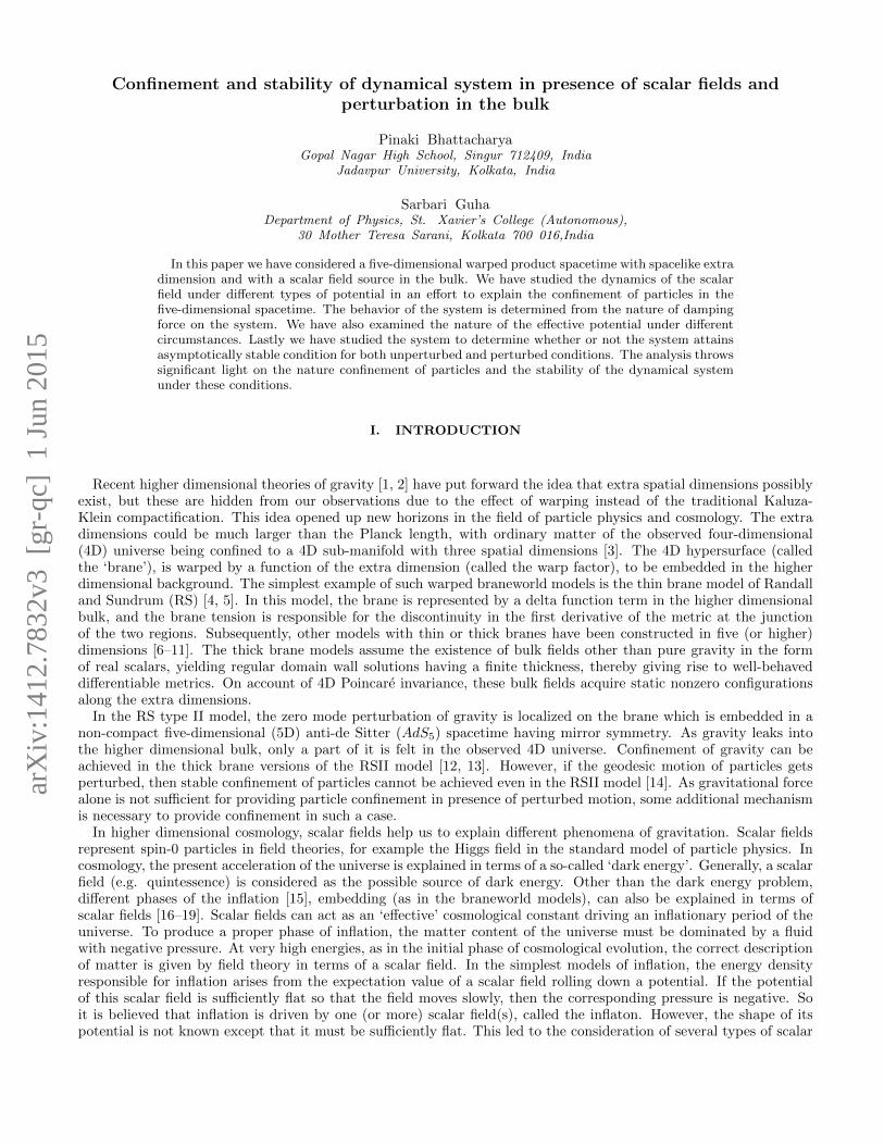
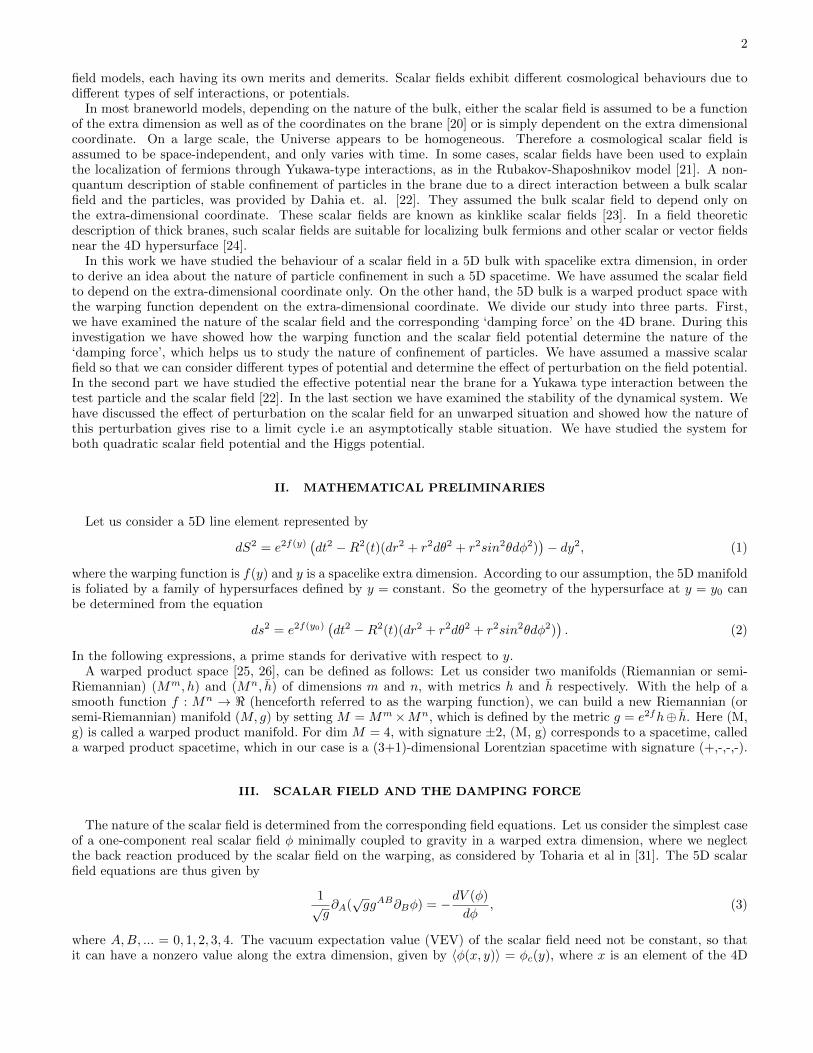
Since we were unable to find the analytical solution for (6), we solved the system in the same way as done in [37]using the NDSolve routine from Mathematica, assuming the boundary condition φ(0) = 1 and φ′(0) = 0. FIG. 1and FIG. 2 shows the nature of the scalar field and the nature of the corresponding damping force under a growingwarping function (f(y) = A ln cosh(y)). We find that the damping force is negative along the extra dimension but itincreases rapidly near the brane. So the figure suggests that as we move towards the y = 0 hypersurface, the systemwill become more stable due to the effect of damping. However this mechanism may not provide efficient trapping ofmatter.

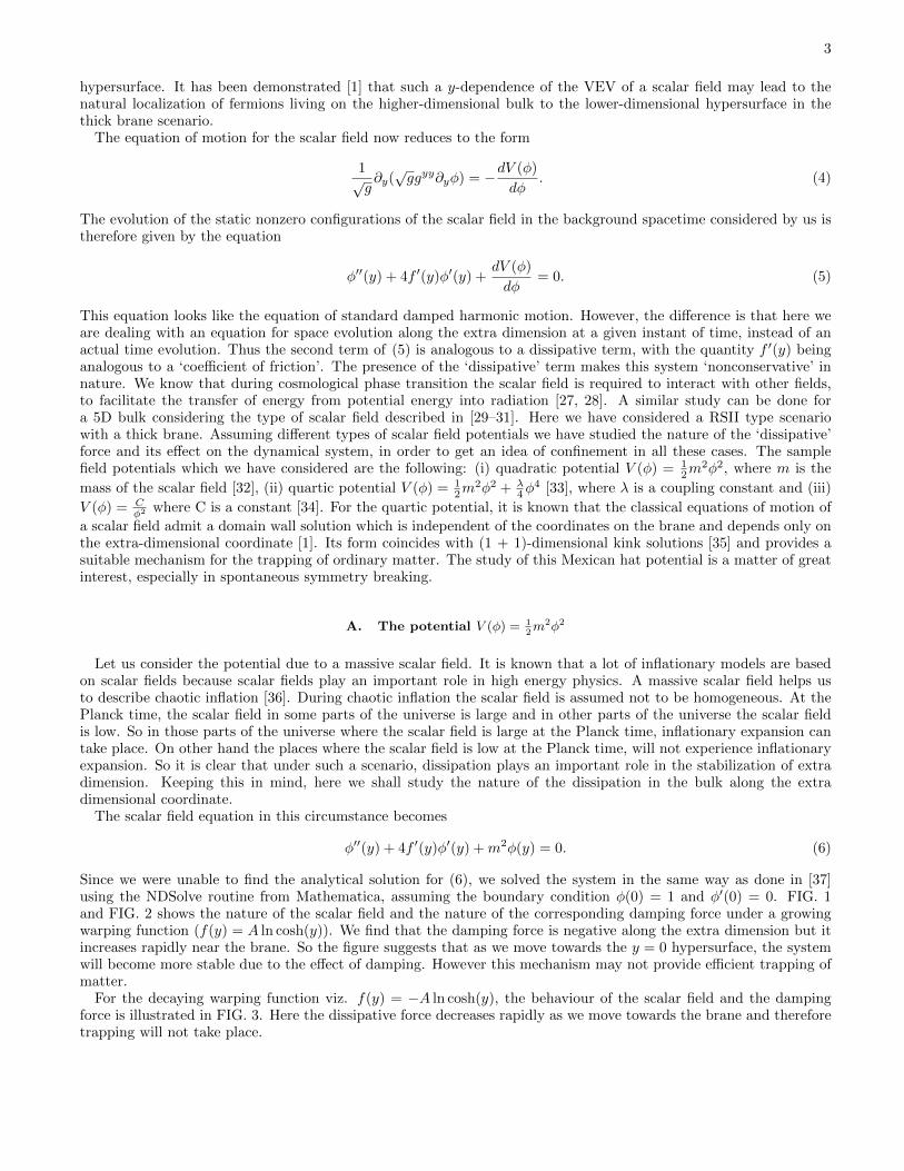
For the decaying warping function viz. f(y) = −A ln cosh(y), the behaviour of the scalar field and the dampingforce is illustrated in FIG. 3. Here the dissipative force decreases rapidly as we move towards the brane and thereforetrapping will not take place.

4

FIG. 1: Figure describing the variation of the scalar fieldwith respect to the extra dimensional coordinate whenV (φ) = 1

2m2φ2 and f(y) = A ln cosh(y).

FIG. 2: Figure showing the variation of the dragging forcewith the extra dimensional coordinate for V (φ) = 1

2m2φ2

and f(y) = A ln cosh(y).

FIG. 3: The figure on the left shows the behaviour of the scalar field (along the vertical axis) and the second one shows thevariation of the damping force (along the vertical) with respect to the extra dimensional coordinate (along the horizontal axis)when V (φ) = 1

2m2φ2 and f(y) = −A ln cosh(y).

B. The potential V (φ) = 12m2φ2 + λ

4φ4

Here we shall consider a single quadratically self coupled scalar field with λ as the coupling constant. We maychoose λ to be either positive or negative. But if we choose a negative coupling constant, then it leads to a potentialwhich has no lower bound. The potential has a single minimum at the origin if we assume that m2 is positive for apositive coupling constant, and it will also remain invariant under Z2 symmetry. But spontaneous symmetry breakingoccurs when m2 is negative [38, 39]. Thus we have considered both positive and negative values of m2 in our analysis.The consideration of spontaneous symmetry breaking can lead to important consequences during the creation andformation of the universe. Symmetry breaking methods can be used to describe the production of particles withoutthe loss of energy and gives rise to the gauge bosons. The field equation under such a potential can be written as

φ′′(y) + 4f ′(y)φ′(y) +m2φ(y) +λ

3φ3(y) = 0. (7)

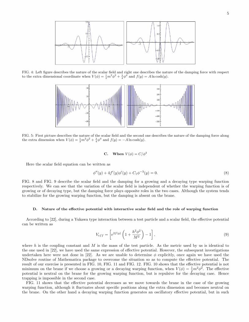
For the growing warping function, FIG. 4 shows that both the field and the damping force are oscillatory in nature,but the oscillations die out gradually as we move away from the brane. The damping vanishes not only on the branebut also at other places along the extra dimension. Thus the system has several unstable points in addition to theone on the brane. In this case we do not expect any efficient confinement of particles on the brane.

In the case of the decaying warping function, both the field and the damping shows oscillatory behaviour (FIG. 5).But unlike the previous case, here the amplitude of oscillations diverge as we move away from the brane. The dampingis absent on the brane.

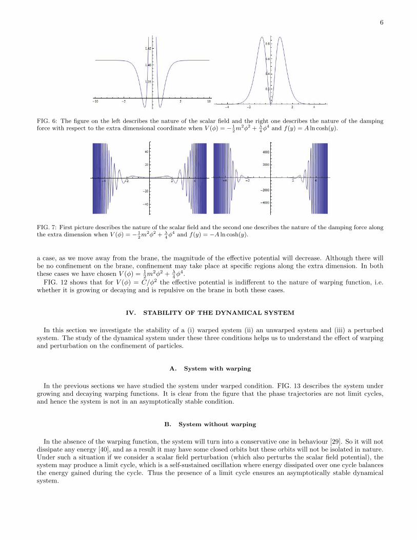
From FIG. 6 it is clear that the presence of negative m2 term implies that the dissipative nature of the systemgradually falls as we move away from the brane in the case of the growing warping function. For the decaying typewarping function, the dissipation is oscillating in nature along the extra dimensional coordinate.

5

FIG. 4: Left figure describes the nature of the scalar field and right one describes the nature of the damping force with respectto the extra dimensional coordinate when V (φ) = 1

2m2φ2 + λ

4φ4 and f(y) = A ln cosh(y).

FIG. 5: First picture describes the nature of the scalar field and the second one describes the nature of the damping force alongthe extra dimension when V (φ) = 1

2m2φ2 + λ

4φ4 and f(y) = −A ln cosh(y).

C. When V (φ) = C/φ2

Here the scalar field equation can be written as

φ′′(y) + 4f ′(y)φ′(y) + C1φ−3(y) = 0. (8)

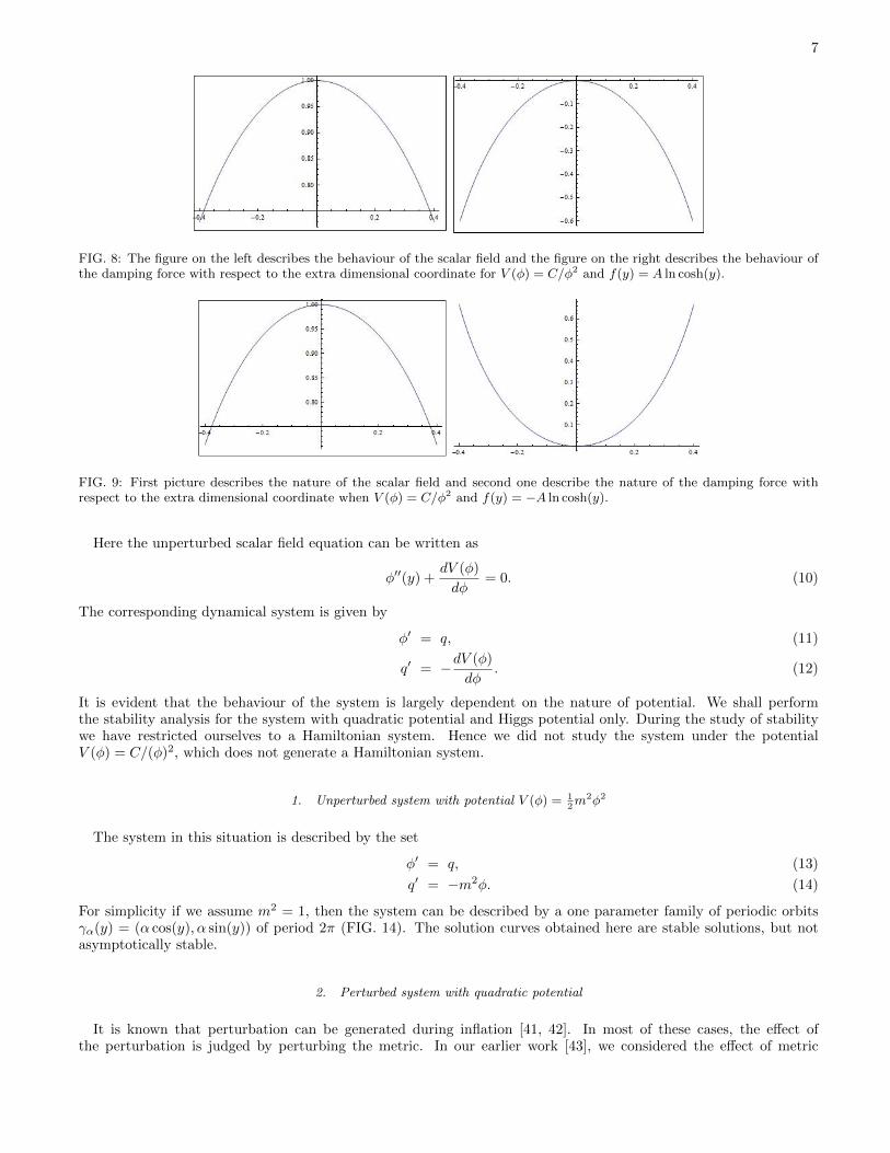
FIG. 8 and FIG. 9 describe the scalar field and the damping for a growing and a decaying type warping functionrespectively. We can see that the variation of the scalar field is independent of whether the warping function is ofgrowing or of decaying type, but the damping force plays opposite roles in the two cases. Although the system tendsto stabilize for the growing warping function, but the damping is absent on the brane.

D. Nature of the effective potential with interactive scalar field and the role of warping function

According to [22], during a Yukawa type interaction between a test particle and a scalar field, the effective potentialcan be written as

Veff =

[e2f(y)

(1 +

h2φ2

M2

)− 1

], (9)

where h is the coupling constant and M is the mass of the test particle. As the metric used by us is identical tothe one used in [22], we have used the same expression of effective potential. However, the subsequent investigationsundertaken here were not done in [22]. As we are unable to determine φ explicitly, once again we have used theNDsolve routine of Mathematica package to overcome the situation so as to compute the effective potential. Theresult of our exercise is presented in FIG. 10, FIG. 11 and FIG. 12. FIG. 10 shows that the effective potential is notminimum on the brane if we choose a growing or a decaying warping function, when V (φ) = 1

2m2φ2. The effective

potential is neutral on the brane for the growing warping function, but is repulsive for the decaying case. Hencetrapping is impossible in the second case.

FIG. 11 shows that the effective potential decreases as we move towards the brane in the case of the growingwarping function, although it fluctuates about specific positions along the extra dimension and becomes neutral onthe brane. On the other hand a decaying warping function generates an oscillatory effective potential, but in such

6

FIG. 6: The figure on the left describes the nature of the scalar field and the right one describes the nature of the dampingforce with respect to the extra dimensional coordinate when V (φ) = − 1

2m2φ2 + λ

4φ4 and f(y) = A ln cosh(y).

FIG. 7: First picture describes the nature of the scalar field and the second one describes the nature of the damping force alongthe extra dimension when V (φ) = − 1

2m2φ2 + λ

4φ4 and f(y) = −A ln cosh(y).

a case, as we move away from the brane, the magnitude of the effective potential will decrease. Although there willbe no confinement on the brane, confinement may take place at specific regions along the extra dimension. In boththese cases we have chosen V (φ) = 1

2m2φ2 + λ

4φ4.

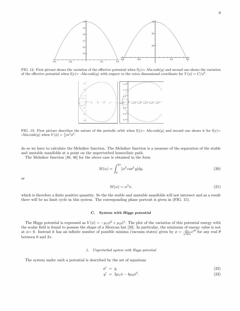
FIG. 12 shows that for V (φ) = C/φ2 the effective potential is indifferent to the nature of warping function, i.e.whether it is growing or decaying and is repulsive on the brane in both these cases.

IV. STABILITY OF THE DYNAMICAL SYSTEM

In this section we investigate the stability of a (i) warped system (ii) an unwarped system and (iii) a perturbedsystem. The study of the dynamical system under these three conditions helps us to understand the effect of warpingand perturbation on the confinement of particles.

A. System with warping

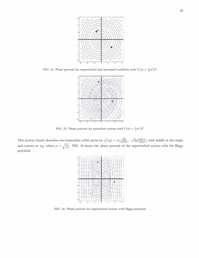
In the previous sections we have studied the system under warped condition. FIG. 13 describes the system undergrowing and decaying warping functions. It is clear from the figure that the phase trajectories are not limit cycles,and hence the system is not in an asymptotically stable condition.

B. System without warping

In the absence of the warping function, the system will turn into a conservative one in behaviour [29]. So it will notdissipate any energy [40], and as a result it may have some closed orbits but these orbits will not be isolated in nature.Under such a situation if we consider a scalar field perturbation (which also perturbs the scalar field potential), thesystem may produce a limit cycle, which is a self-sustained oscillation where energy dissipated over one cycle balancesthe energy gained during the cycle. Thus the presence of a limit cycle ensures an asymptotically stable dynamicalsystem.

7

FIG. 8: The figure on the left describes the behaviour of the scalar field and the figure on the right describes the behaviour ofthe damping force with respect to the extra dimensional coordinate for V (φ) = C/φ2 and f(y) = A ln cosh(y).

FIG. 9: First picture describes the nature of the scalar field and second one describe the nature of the damping force withrespect to the extra dimensional coordinate when V (φ) = C/φ2 and f(y) = −A ln cosh(y).

Here the unperturbed scalar field equation can be written as

φ′′(y) +dV (φ)

dφ= 0. (10)

The corresponding dynamical system is given by

φ′ = q, (11)

q′ = −dV (φ)

dφ. (12)

It is evident that the behaviour of the system is largely dependent on the nature of potential. We shall performthe stability analysis for the system with quadratic potential and Higgs potential only. During the study of stabilitywe have restricted ourselves to a Hamiltonian system. Hence we did not study the system under the potentialV (φ) = C/(φ)2, which does not generate a Hamiltonian system.

1. Unperturbed system with potential V (φ) = 12m2φ2

The system in this situation is described by the set

φ′ = q, (13)

q′ = −m2φ. (14)

For simplicity if we assume m2 = 1, then the system can be described by a one parameter family of periodic orbitsγα(y) = (α cos(y), α sin(y)) of period 2π (FIG. 14). The solution curves obtained here are stable solutions, but notasymptotically stable.

2. Perturbed system with quadratic potential

It is known that perturbation can be generated during inflation [41, 42]. In most of these cases, the effect ofthe perturbation is judged by perturbing the metric. In our earlier work [43], we considered the effect of metric

8

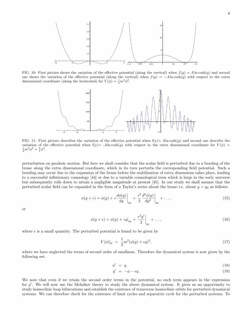
FIG. 10: First picture shows the variation of the effective potential (along the vertical) when f(y) = A ln cosh(y) and secondone shows the variation of the effective potential (along the vertical) when f(y) = −A ln cosh(y) with respect to the extradimensional coordinate (along the horizontal) for V (φ) = 1

2m2φ2.

FIG. 11: First picture describes the variation of the effective potential when f(y)= Aln cosh(y) and second one describe thevariation of the effective potential when f(y)= -Aln cosh(y) with respect to the extra dimensional coordinate for V (φ) =12m2φ2 + λ

4φ4.

perturbation on geodesic motion. But here we shall consider that the scalar field is perturbed due to a bending of thebrane along the extra dimensional coordinate, which in its turn perturbs the corresponding field potential. Such abending may occur due to the expansion of the brane before the stabilization of extra dimensions takes place, leadingto a successful inflationary cosmology [44] or due to a variable cosmological term which is large in the early universebut subsequently rolls down to attain a negligible magnitude at present [45]. In our study we shall assume that theperturbed scalar field can be expanded in the form of a Taylor’s series about the brane i.e. about y = y0 as follows:

φ(y + ε) = φ(y) + εdφ(y)

dy

∣∣∣∣y0

+ε2

2

d2φ(y)

dy2

∣∣∣∣y0

+ . . . , (15)

or

φ(y + ε) = φ(y) + εq|y0 +ε2q′

2

∣∣∣∣y0

+ . . . , (16)

where ε is a small quantity. The perturbed potential is found to be given by

V (φ)|p =1

2m2(φ(y) + εq)2, (17)

where we have neglected the terms of second order of smallness. Therefore the dynamical system is now given by thefollowing set:

φ′ = q, (18)

q′ = −φ− εq. (19)

We note that even if we retain the second order terms in the potential, no such term appears in the expressionfor q′. We will now use the Melnikov theory to study the above dynamical system. It gives us an opportunity tostudy homoclinic loop bifurcations and establish the existence of transverse homoclinic orbits for perturbed dynamicalsystems. We can therefore check for the existence of limit cycles and separatrix cycle for the perturbed systems. To

9

FIG. 12: First picture shows the variation of the effective potential when f(y)= Aln cosh(y) and second one shows the variationof the effective potential when f(y)= -Aln cosh(y) with respect to the extra dimensional coordinate for V (φ) = C/φ2.

FIG. 13: First picture describes the nature of the periodic orbit when f(y)= Aln cosh(y) and second one shows it for f(y)=-Aln cosh(y) when V (φ) = 1

2m2φ2.

do so we have to calculate the Melnikov function. The Melnikov function is a measure of the separation of the stableand unstable manifolds at a point on the unperturbed homoclinic path.

The Melnikov function [40, 46] for the above case is obtained in the form

M(α) =

∫ 2π

0

[α2 cos2 y]dy, (20)

or

M(α) = α2π, (21)

which is therefore a finite positive quantity. So the the stable and unstable manifolds will not intersect and as a resultthere will be no limit cycle in this system. The corresponding phase portrait is given in (FIG. 15).

C. System with Higgs potential

The Higgs potential is expressed as V (φ) = −µ1φ2 + µ2φ

4. The plot of the variation of this potential energy withthe scalar field is found to possess the shape of a Mexican hat [33]. In particular, the minimum of energy value is notat φ= 0. Instead it has an infinite number of possible minima (vacuum states) given by φ = µ1√

2µ2eiθ for any real θ

between 0 and 2π.

1. Unperturbed system with Higgs potential

The system under such a potential is described by the set of equations

φ′ = q, (22)

q′ = 2µ1φ− 4µ2φ3. (23)

10

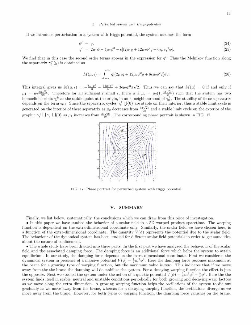
FIG. 14: Phase portrait for unperturbed and unwarped condition with V (φ) = 12m2φ2.

FIG. 15: Phase portrait for perturbed system with V (φ) = 12m2φ2.

This system clearly describes two homoclinic orbits given by γ±0 (y) = ±(√2p

cosh y ,−√

2p tanh ycosh y ), with saddle at the origin

and centers at ±p, where p =√

µ1

µ2. FIG. 16 shows the phase portrait of the unperturbed system with the Higgs

potential.

FIG. 16: Phase portrait for unperturbed system with Higgs potential.

11

2. Perturbed system with Higgs potential

If we introduce perturbation in a system with Higgs potential, the system assumes the form

φ′ = q, (24)

q′ = 2µ1φ− 4µ2φ3 − ε[(2µ1q + 12µ2φ

2q + 6εµ2q2φ]. (25)

We find that in this case the second order terms appear in the expression for q′. Thus the Melnikov function alongthe separatrix γ+0 (y) is obtained as

M(µ, ε) =

∫ ∞−∞

q[(2µ1q + 12µ2φ2q + 6εµ2q

2φ]dy. (26)

This integral gives us M(µ, ε) = − 8µ1p2

3 − 64µ2p4

5 + 3εµ2p3π√

2. Thus we can say that M(µ) = 0 if and only if

µ1 = µ233√2ε

98 . Therefore for all sufficiently small ε, there is a µε = µ2(1, 33√2ε

98 ) such that the system has two

homoclinic orbits γ±ε at the saddle point at the origin, in an ε- neighbourhood of γ±0 . The stability of these separatrixdepends on the term εµ1. Since the separatrix cycles γ±ε

⋃{0} are stable on their interior, thus a stable limit cycle is

generated on the interior of these separatrix as µ2 decreases from 33√2ε

98 and a stable limit cycle on the exterior of the

graphic γ+ε⋃γ−ε⋃{0} as µ1 increases from 33

√2ε

98 . The corresponding phase portrait is shown in FIG. 17.

FIG. 17: Phase portrait for perturbed system with Higgs potential.

V. SUMMARY

Finally, we list below, systematically, the conclusions which we can draw from this piece of investigation.• In this paper we have studied the behavior of a scalar field in a 5D warped product spacetime. The warping

function is dependent on the extra-dimensional coordinate only. Similarly, the scalar field we have chosen here, isa function of the extra-dimensional coordinate. The quantity V (φ) represents the potential due to the scalar field.The behaviour of the dynamical system has been studied for different scalar field potentials in order to get some ideaabout the nature of confinement.• The whole study have been divided into three parts. In the first part we have analyzed the behaviour of the scalar

field and the associated damping force. The damping force is an additional force which helps the system to attainequilibrium. In our study, the damping force depends on the extra dimensional coordinate. First we considered thedynamical system in presence of a massive potential V (φ) = 1

2m2φ2. Here the damping force becomes maximum at

the brane for a growing type of warping function, but the maximum value is zero. This indicates that if we moveaway from the the brane the damping will de-stabilize the system. For a decaying warping function the effect is justthe opposite. Next we studied the system under the action of a quartic potential V (φ) = 1

2m2φ2 + λ

4φ4. Here the the

system finds itself in stable, neutral and unstable conditions periodically for both growing and decaying warp factorsas we move along the extra dimension. A growing warping function helps the oscillations of the system to die outgradually as we move away from the brane, whereas for a decaying warping function, the oscillations diverge as wemove away from the brane. However, for both types of warping function, the damping force vanishes on the brane.

12

Lastly we have studied the effect of the potential V (φ) = C/φ2. Here the nature of the scalar field remains almostthe same for both growing and decaying warping functions, as if the field is indifferent to the warp factor, though thecorresponding damping force shows opposite behaviour in these two cases. Although the system tends to stabilize forthe growing warping function, but the damping is absent on the brane.• In the second part we have assumed the scalar field to have Yukawa-type interaction with the test particle. Under

this condition we have studied the effective potential, which shows a double bottom nature for growing and decayingwarping functions when the scalar field has a massive quadratic potential. For a quartic potential, in the case of agrowing warping function, the effective potential becomes minimum at the brane, but the minimum value is zero,indicating neutral confinement. Whereas for the decaying warping function it attains a repulsive maximum on thebrane. But the interesting part appears when we choose V (φ) = C/φ2. The behaviour of the effective potential onthe brane is identical for both the warping functions, and is repulsive in nature. This shows that the system ignoresthe presence of growing and decaying warping functions in the presence of this scalar field potential.• In the final part we have studied the stability of the dynamical system in presence and absence of a perturbation

during an unwarped condition. We found that the presence of perturbation may or may not generate asymptoticallystable cycle i.e a limit cycle, depending on the nature of the scalar field potential. In the warped condition, the phasetrajectories are not limit cycles and therefore we need not analyze the stability of the system in this condition. In theunwarped case, for the quadratic potential we find that there is a condition on the possibility of obtaining a limit cyclewhen the system remains unperturbed. So we conclude that there is a restriction on the situation when the systemcan become asymptotically stable. For the perturbed system the stable and unstable manifolds does not intersect andas a result there will be no limit cycle. During the study of the Higgs potential we found that we may obtain stableand unstable limit cycles.

Summarising we can say that the above analysis throws new light on the issue of confinement in presence of scalarfields in the bulk 5D spacetime for different types of scalar field potentials. The nature of the dissipation has beenstudied to see the role of dissipative term in confinement. During the study of the conservative system we haveconsidered the effect of a perturbation to see whether, and under what condition dissipation comes into play in thesystem. To do so we determined the condition to get a limit cycle which indicates an asymptotically stable dynamicalsystem.

Acknowledgments

SG thanks IUCAA, India for an associateship. PB gratefully acknowledges the facilities available at the Departmentof Physics, St. Xavier’s College (Autonomous), Kolkata and the Relativity and Cosmology Research Center, JadavpurUniversity.

[1] V. A. Rubakov and M. E. Shaposhnikov, Phys. Lett. B 125, 136 (1983).[2] J. Scherk and J.H. Schwarz, Phys. Lett. B 57, 463 (1975); E. Witten, Nucl. Phys. B 186, 412 (1981).[3] N. Arkani-Hamed, S. Dimopoulos, G. Dvali, Phys.Lett. B 429, 263 (1998); I. Antoniadis, N. Arkani-Hamed, S. Dimopoulos,

G. Dvali, Phys. Lett. B 436, 257 (1998); N. Arkani-Hamed, S. Dimopoulos and G. Dvali, Phys. Rev. D 59, 086004 (1999).[4] L. Randall and R. Sundrum, Phys. Rev. Lett. 83, 3370 (1999).[5] L. Randall and R. Sundrum, Phys. Rev. Lett. 83, 4690 (1999).[6] R. Koley and S. Kar, Class. Quant. Grav. 22, 753 (2005).[7] M. Giovannini, Class. Quant. Grav. 20, 1063 (2003).[8] S. Guha and S Chakraborty, Gen. Relativ. Gravit. 42, 1739 (2010).[9] P. Bhattacharya and S Guha, Phys. Scr. 85, 025001 (2012).

[10] D. Youm, Phys. Rev. D 62, 084002 (2000).[11] S. S. Seahra, Phys. Rev. D 68, 104027 (2003).[12] O. De Wolfe, D.Z. Freedman, S.S. Gubser, A. Karch, Phys. Rev. D 62, 046008 (2000).[13] A. Chamblin, G.W. Gibbons, Phys. Rev. Lett. 84, 1090 (2000).[14] W. Muck, K.S. Viswanathan and I. Volovich, Phys. Rev. D 62, 105019 (2000).[15] A. Linde, Particle Physics and Inflationary Cosmology (CRC Press, Florida, 1990).[16] Damien P. George, M. Trodden and R. R. Volkas, Journal of High Energy Physics 02(2009)035.[17] P. S. Wesson, arXiv:1003.2476[gr-qc].[18] E. Anderson, F. Dahia, J. E. Lidsey and C. Romero, J.Math.Phys. 44, 5108 (2003).[19] A. Macias and J. L. C-Cota, C. Lammerzahl, Exact Solutions and Scalar Fields in Gravity, (Kluwer Academic Publishers,

New York, 2002).[20] S. Pal and S. Kar, Gen. Relativ .Gravit. 41, 1165 (2009).

13

[21] V. A. Rubakov, Phys. Usp. 44, 871 (2001); Usp. Fiz. Nauk 171, 913 (2001).[22] F. Dahia and C. Romero, Phys. Lett. B 651, 232 (2007).[23] N. Arkani-Hamed and M. Schmaltz, Phys. Rev. D 61, 033005 (2000); D. E. Kaplan and T. M. Tait, Journal of High Energy

Physics 11(2001)051.[24] R. Davies, D. P. George, and R. R. Volkas, Phys. Rev. D 77, 124038 (2008).[25] J. Carot and J. da Costa, Class. Quantum Grav. 10, 461 (1993).[26] R. L. Bishop and B. O. ONeill, Trans. Am. Math. Soc. 145, 1 (1969).[27] Sam Bartrum, Mar Bastero-Gil, Arjun Berera, Rafael Cerezo, Rudnei O. Ramos, Joao G. Rosa, Phys. Lett. B 732, 116

(2014); Sam Bartrum, Arjun Berera, Joao G. Rosa, arXiv:1412.5489.[28] A Berera, Dissipative Dynamics of Inflation, arXiv:hep-ph/0106310v2.[29] Manuel Toharia and Mark Trodden, Phys. Rev. Lett 100, 041602 (2008).[30] Manuel Toharia and Mark Trodden, Phys. Rev. D 77, 025029 (2008).[31] Manuel Toharia and Mark Trodden, Phys. Rev. D 82, 025009 (2010).[32] L.N. Granda, J.C.A.P. 04(2011)016.[33] J. W. Moffat, Int. Jour. Mod. Phys. D 12, 1279 (2003).[34] A. Ghalee, arXiv:1402.6798 [astro-ph.CO]; Phys. Lett. B 724, 198 (2013).[35] R. Dashen, B. Hasslacher and A. Neveu, Phys. Rev. D 10, 4130 (1974).[36] Andrei Linde, arXiv:hep-th/0503203v1 26 Mar 2005[37] V. Dzhunushaliev, V. Folomeev, D. Singleton and S. Aguilar-Rudametkin, Phys. Rev. D 77, 044006 (2008).[38] R.Brout, F.Englert, E.Gunzig, The creation of the universe as a quantum phenomenon,Annals of Physics. Vol 115, page

78.[39] Amin Akhavan, arXiv:1403.0198v1 [hep-th] 2 Mar 2014[40] D. W. Jordan and P. Smith, Nonlinear Ordinary Differential Equations: An introduction for Scientists and Engineers, 4th

ed. (Oxford University Press Inc., New York, 2007).[41] L. Amendola and S. Tsujikwwa, DARK ENERGY: Theory and Observations, (Cambridge University Press, Cambridge,

UK, 2010).[42] A. Riotto, Inflation and the theory of cosmological perturbations, arXiv:hep-ph/0210162.[43] P. Bhattacharya and S Guha, arXiv:1202.2328v4 [gr-qc] 1 Jun 2015.[44] N. Kaloper, Phys. Rev. D 60, 123506 (1999).[45] M. D. Maia and G. S. Silva, Phys. Rev. D 50, 7233 (1994).[46] L. Perko, Differential Equations and Dynamical Systems, 3rd ed. (Springer-Verlag, New York. Inc., 2001).