Goodwin, Graebe, Salgado ©, Prentice Hall 2000 Chapter 8 Fundamental Design Limitations in SISO Control

Goodwin, Graebe, Salgado ©, Prentice Hall 2000Chapter 8

Chapter 8

Fundamental Design Fundamental Design Limitations in SISO ControlLimitations in SISO Control


This chapter examines those issues that limit the achievable performance in control systems. The limitations that we examine here include Sensors Actuators

maximal movements minimal movements

Model deficiencies Structural issues, including

poles in the ORHP zeros in the ORHP zeros that are stable but close to the origin poles on the imaginary axis zeros on the imaginary axis.


An understanding of these limitations is central to understanding control system design. Indeed, it is often more important to know what cannot be achieved (and why) than it is to generate a particular solution to a given problem.


Sensors

Sensors are a crucial part of any control system design, since they provide the necessary information upon which the controller action is based. They are the eyes of the controller. Hence, any error, or significant defect, in the measurement system will have a significant impact on performance.


Noise

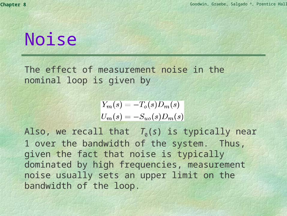
The effect of measurement noise in the nominal loop is given by

Also, we recall that T0(s) is typically near 1 over the bandwidth of the system. Thus, given the fact that noise is typically dominated by high frequencies, measurement noise usually sets an upper limit on the bandwidth of the loop.


Actuators

If sensors provide the eyes of control, then actuators provide the muscle. However, actuators are also a source of limitations in control performance. We will examine two aspects of actuator limitations. These are maximal movement, and minimal movement.


Maximal Actuator Movement

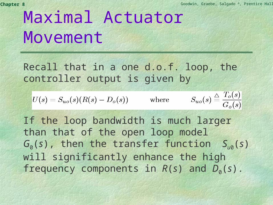
Recall that in a one d.o.f. loop, the controller output is given by

If the loop bandwidth is much larger than that of the open loop model G0(s), then the transfer function Su0(s) will significantly enhance the high frequency components in R(s) and D0(s).


Example:

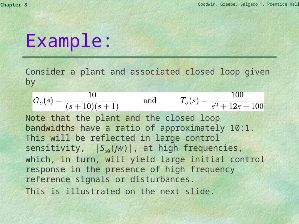
Consider a plant and associated closed loop given by

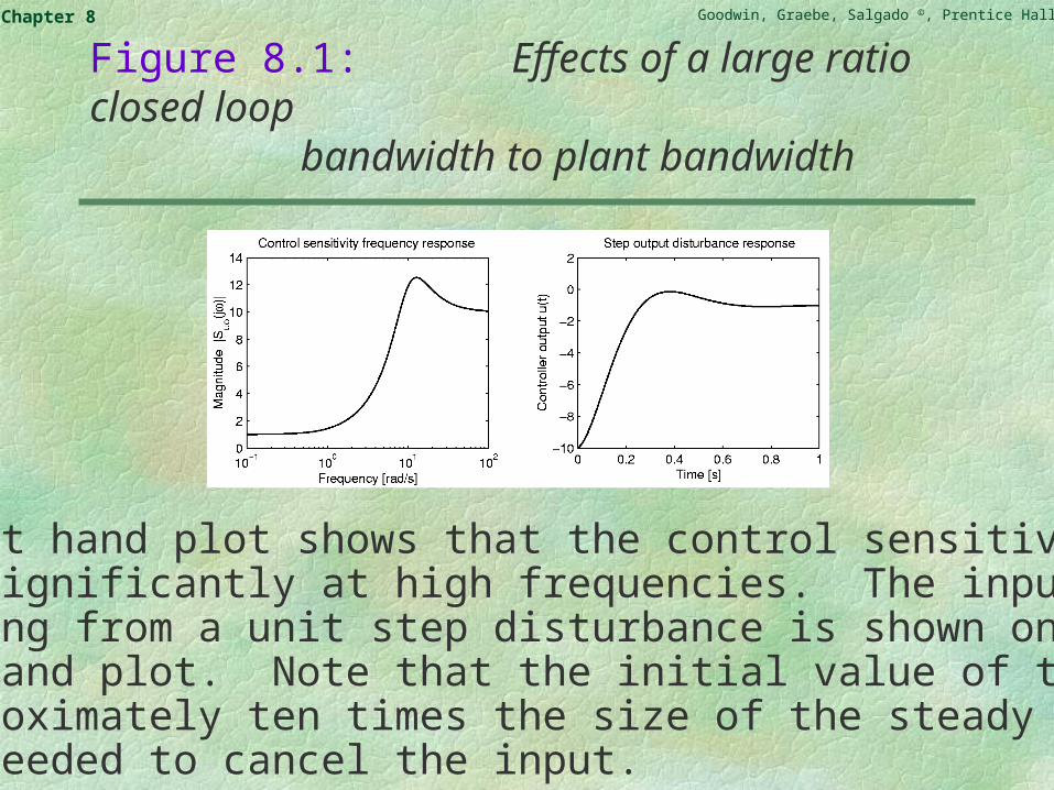
Note that the plant and the closed loop bandwidths have a ratio of approximately 10:1. This will be reflected in large control sensitivity, |Su0(jw)|, at high frequencies, which, in turn, will yield large initial control response in the presence of high frequency reference signals or disturbances.

This is illustrated on the next slide.


Figure 8.1: Effects of a large ratio closed loop bandwidth to plant bandwidth

The left hand plot shows that the control sensitivitygrows significantly at high frequencies. The input signalresulting from a unit step disturbance is shown on the right hand plot. Note that the initial value of the inputis approximately ten times the size of the steady stateinput needed to cancel the input.


Conclusion:

To avoid actuator saturation or slew rate problems, it will generally be necessary to place an upper limit

on the closed loop bandwidth.


Minimal Actuator Movement

We learned above that control loop performance is limited by the maximal available movement available from actuators. This is heuristically responsible. What is perhaps less obvious is that control systems are often also limited by minimal actuator movements.


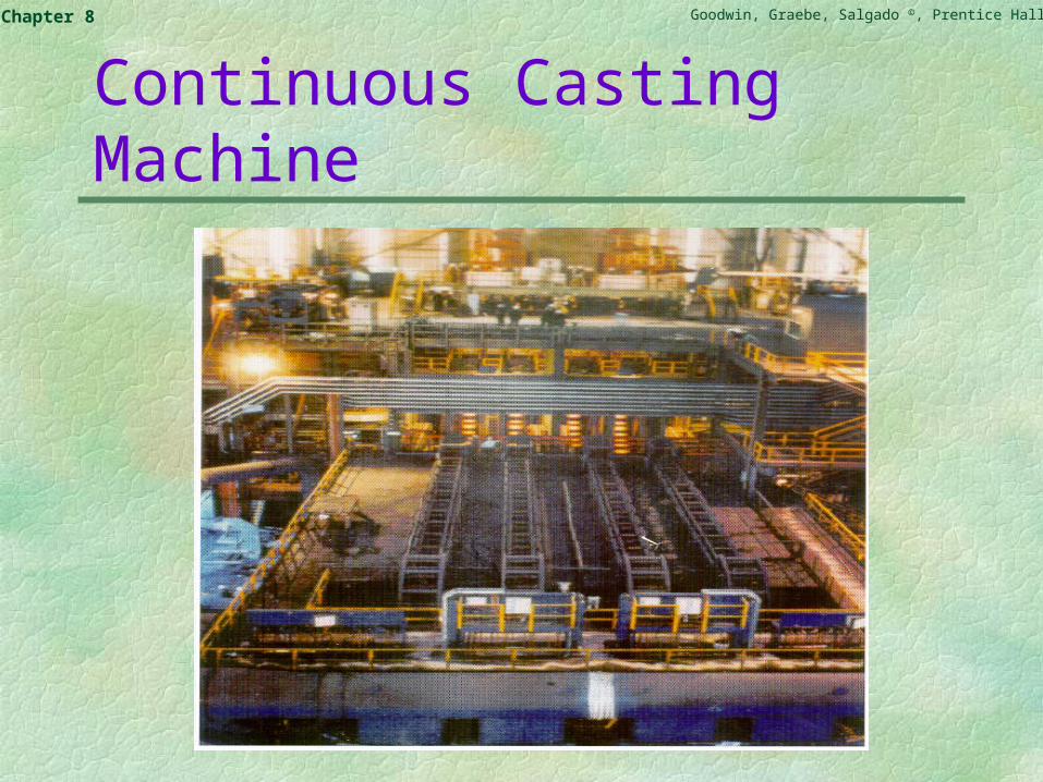
Example: Continuous Casting

Consider again the mould level controller illustrated in the following slides. It is known that many mould level controllers in industry exhibit poor performances in the form of self-sustaining oscillations. See for example the real data shown in Figure 8.2. Many explanations have been proposed for this problem. However, at least on the system with which the authors are familiar, the difficulty was directly traceable to minimal movement issues associated with the actuator. (The slide gate valve)


Continuous Casting Machine


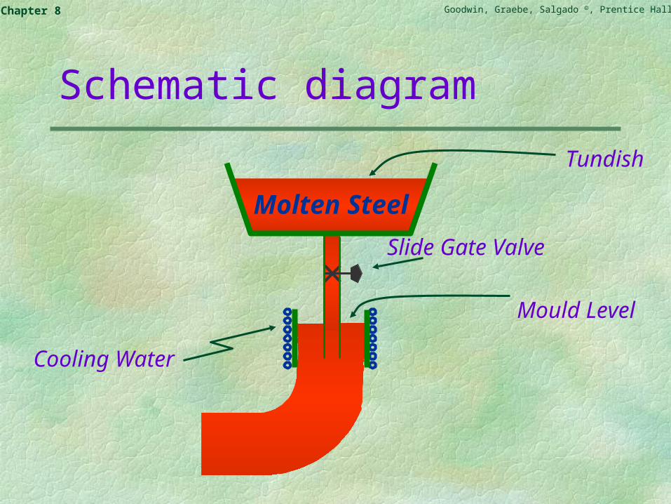
Schematic diagram

Tundish

Slide Gate Valve

Molten Steel

Mould Level

Cooling Water


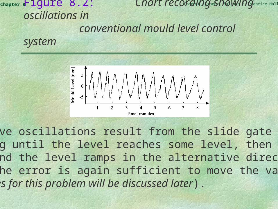
Figure 8.2: Chart recording showing oscillations in

conventional mould level control system

The above oscillations result from the slide gate valvesticking until the level reaches some level, then the valvemoves and the level ramps in the alternative directionuntil the error is again sufficient to move the valve.(Remedies for this problem will be discussed later).


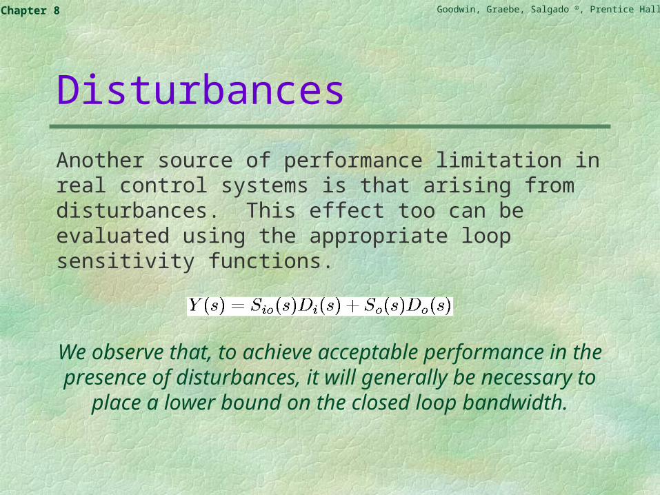
Disturbances

Another source of performance limitation in real control systems is that arising from disturbances. This effect too can be evaluated using the appropriate loop sensitivity functions.

We observe that, to achieve acceptable performance in the presence of disturbances, it will generally be

necessary to place a lower bound on the closed loop bandwidth.


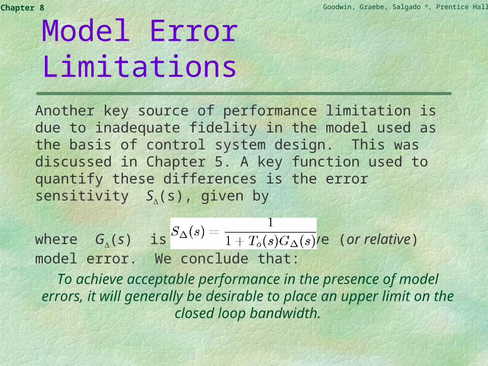
Model Error LimitationsAnother key source of performance limitation is due to inadequate fidelity in the model used as the basis of control system design. This was discussed in Chapter 5. A key function used to quantify these differences is the error sensitivity S(s), given by

where G(s) is the multiplicative (or relative) model error. We conclude that:

To achieve acceptable performance in the presence of model errors, it will generally be desirable to place an upper limit on the

closed loop bandwidth.


Structural Limitations

The above analysis of limitations has focussed on issues arising from the actuators, sensors and model accuracy. However, there is another source of errors arising from the nature of the plant. Specifically we have:

General Ideas: Performance in the nominal linear control loop is also subject to unavoidable constraints which derive from the particular structure of the nominal model itself. We discuss:

delays open loop zeros open loop poles


Delays

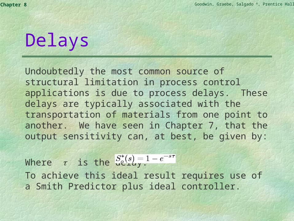
Undoubtedly the most common source of structural limitation in process control applications is due to process delays. These delays are typically associated with the transportation of materials from one point to another. We have seen in Chapter 7, that the output sensitivity can, at best, be given by:

Where is the delay.

To achieve this ideal result requires use of a Smith Predictor plus ideal controller.


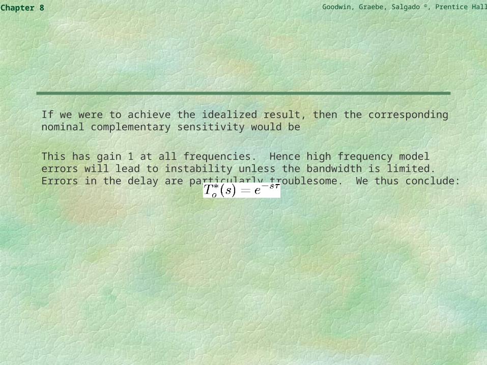
If we were to achieve the idealized result, then the corresponding nominal complementary sensitivity would be

This has gain 1 at all frequencies. Hence high frequency model errors will lead to instability unless the bandwidth is limited. Errors in the delay are particularly troublesome. We thus conclude:


(i) Delays limit disturbance rejection by requiring that a delay occur before the disturbance can be cancelled. This is reflected in the ideal sensitivity S0

*(s);

(ii) Delays further limit the achievable bandwidth due to the impact of model errors.


An interesting question which arises in this context is whether it is worthwhile using a Smith Predictor in practice.

The answer is probably yes if the system model (especially the delay) are accurately known. However, if the delay is poorly known, then robustness considerations limit the achievable bandwidth even if a Smith Predictor is used. Specifically, if the delay is known to say 100%, then the bandwidth is limited to the order of 1/ . Say =1/3, then this gives a bandwidth of approximately 3/. On the other hand, a simple PID controller can probably achieve a bandwidth of 4/. Thus, one can see that accurate knowledge of the system model and delay is a precursor to gaining advantages from using a Smith Predictor.


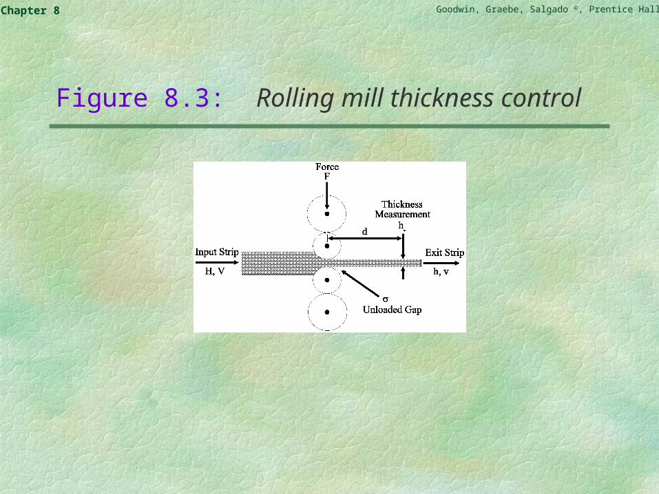
Example 8.3: Thickness control in rolling mills

We recall the example of thickness control in rolling mills as mentioned in Chapter 1 (see next slide for photo). A schematic diagram for one stand of a rolling mill is given in Figure 8.3.In Figure 8.3 we have used the following symbols:

F - Roll Force - unloaded roll gap H - input thickness V - input velocityh - exit thickness), v - exit velocity hm - measured exit thickness, d - distance from mill to exit thickness measurement.

The distance from the mill to output thickness measurement introduces a (speed dependent) time delay of (d/v). This introduces a fundamental limit to the controlled performances as described above.


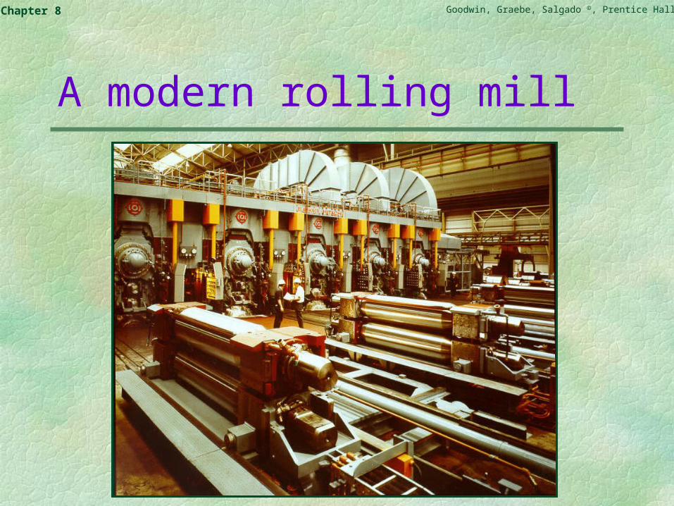
A modern rolling mill


Figure 8.3: Rolling mill thickness control


Open Loop Poles and Zeros

We next study the effect of open loop poles and zeros on achievable performance. We shall see that open loop poles and zeros have a dramatic (and predictable) effect on closed loop performance.

We begin by examining the so-called interpolation constraints which show how open loop poles and zeros are reflected in the poles and zeros of the various closed loop sensitivity functions.


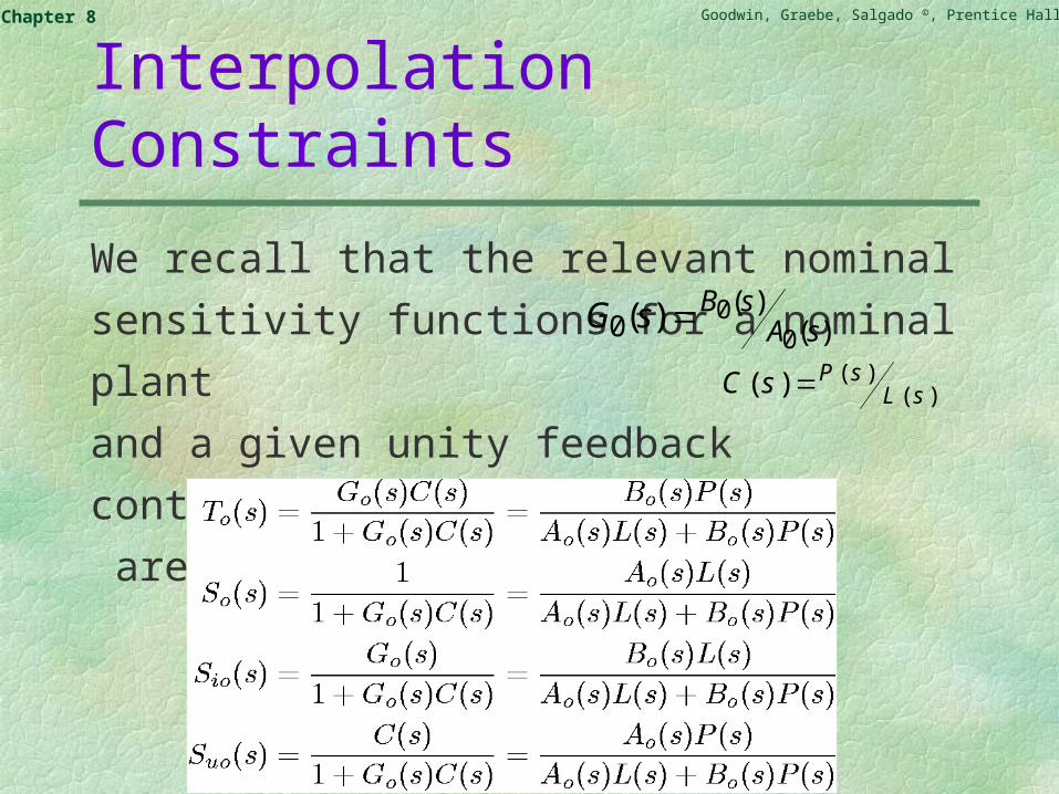
Interpolation Constraints

We recall that the relevant nominal sensitivity

functions for a nominal plant

and a given unity feedback controller

are given below

)()(

0 00)( sA

sBsG

)()()( sL

sPsC


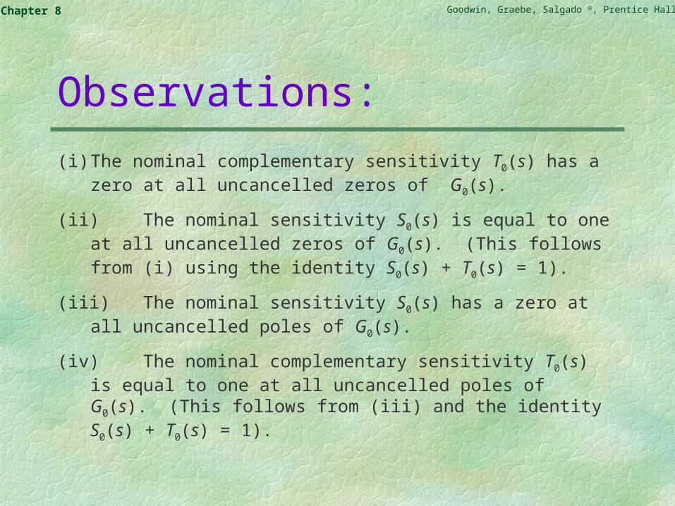
Observations:

(i) The nominal complementary sensitivity T0(s) has a zero at all uncancelled zeros of G0(s).

(ii) The nominal sensitivity S0(s) is equal to one at all uncancelled zeros of G0(s). (This follows from (i) using the identity S0(s) + T0(s) = 1).

(iii) The nominal sensitivity S0(s) has a zero at all uncancelled poles of G0(s).

(iv) The nominal complementary sensitivity T0(s) is equal to one at all uncancelled poles of G0(s). (This follows from (iii) and the identity S0(s) + T0(s) = 1).


We next show how these interpolation constraints lead to performance limits.


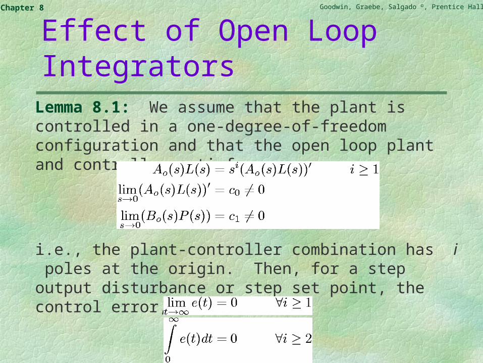
Effect of Open Loop IntegratorsLemma 8.1: We assume that the plant is controlled in a one-degree-of-freedom configuration and that the open loop plant and controller satisfy:

i.e., the plant-controller combination has i poles at the origin. Then, for a step output disturbance or step set point, the control error, e(t) satisfies


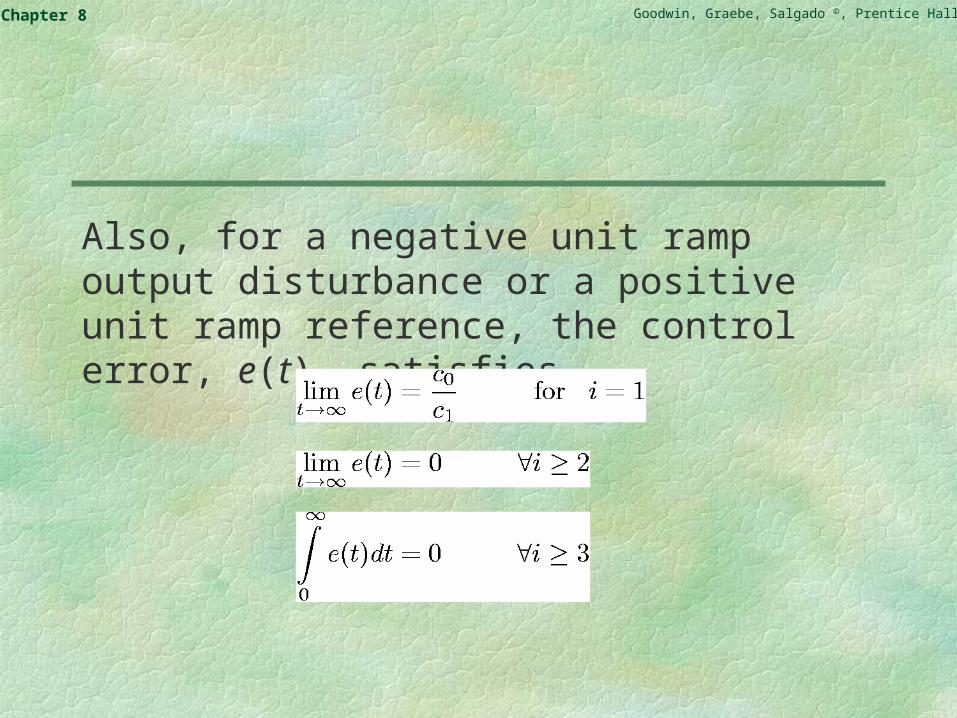
Also, for a negative unit ramp output disturbance or a positive unit ramp reference, the control error, e(t), satisfies


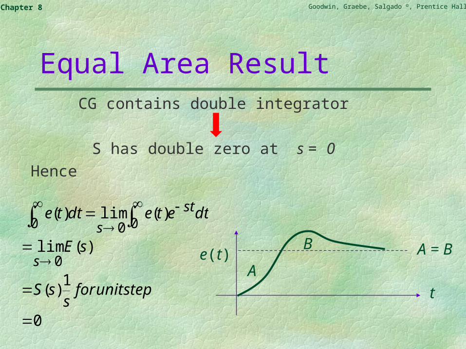
Equal Area ResultCG contains double integrator

S has double zero at s = 0

Hence

0

1)(

)(lim

)(lim)(

0

00 0

stepunitfors

sS

sE

dtetedtte

s

st

s

e(t)B

A

A = B

t


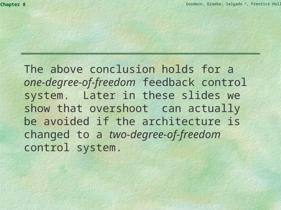
The above conclusion holds for a one-degree-of-freedom feedback control system. Later in these slides we show that overshoot can actually be avoided if the architecture is changed to a two-degree-of-freedom control system.


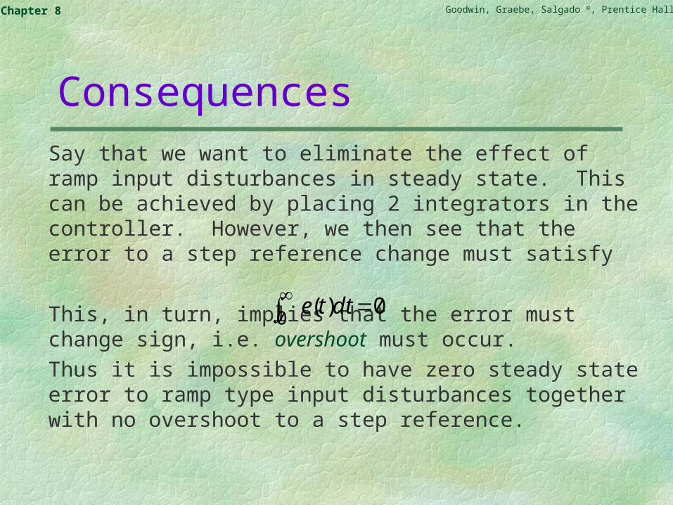
Consequences

Say that we want to eliminate the effect of ramp input disturbances in steady state. This can be achieved by placing 2 integrators in the controller. However, we then see that the error to a step reference change must satisfy

This, in turn, implies that the error must change sign, i.e. overshoot must occur.

Thus it is impossible to have zero steady state error to ramp type input disturbances together with no overshoot to a step reference.

0

0)( dtte


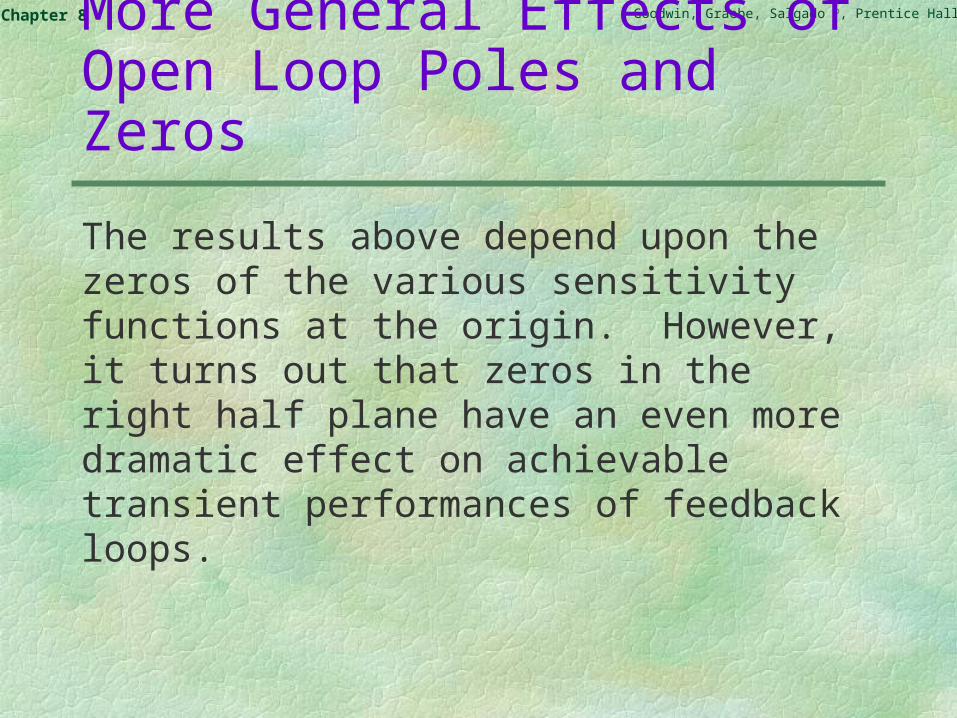
More General Effects of Open Loop Poles and Zeros

The results above depend upon the zeros of the various sensitivity functions at the origin. However, it turns out that zeros in the right half plane have an even more dramatic effect on achievable transient performances of feedback loops.


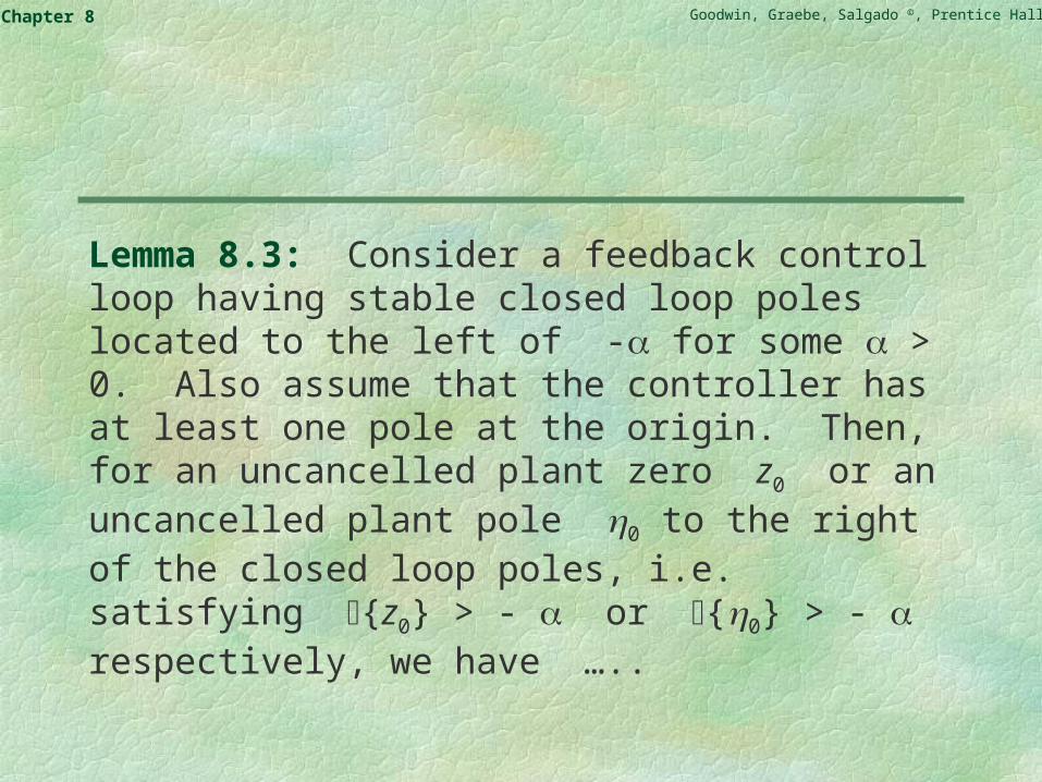
Lemma 8.3: Consider a feedback control loop having stable closed loop poles located to the left of - for some > 0. Also assume that the controller has at least one pole at the origin. Then, for an uncancelled plant zero z0 or an uncancelled plant pole 0 to the right of the closed loop poles, i.e. satisfying {z0} > - or {0} > - respectively, we have …..


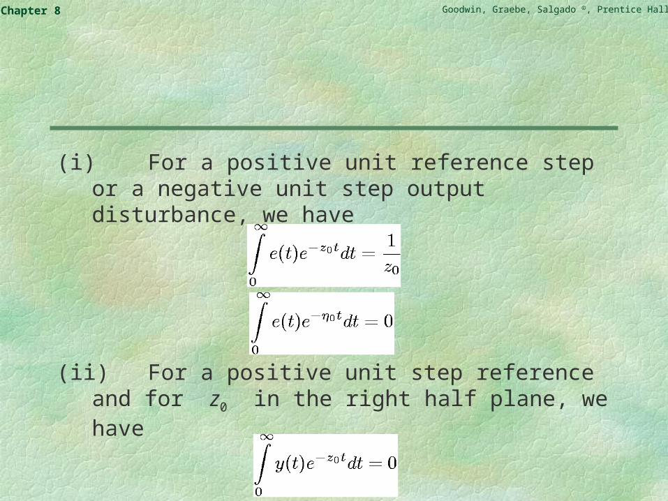
(i) For a positive unit reference step or a negative unit step output disturbance, we have

(ii) For a positive unit step reference and for z0 in the right half plane, we have


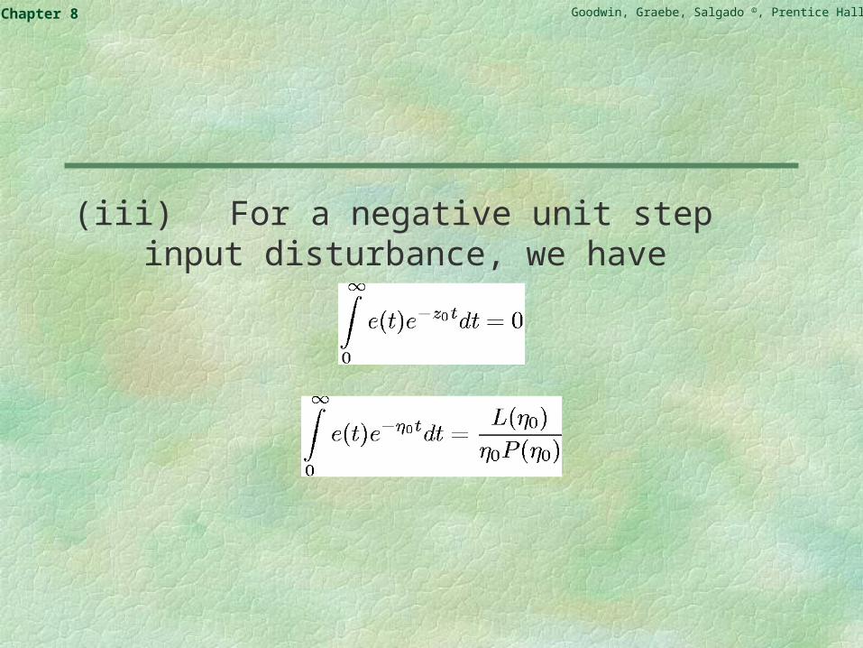
(iii) For a negative unit step input disturbance, we have


Observations

The above integral constraints show that (irrespective of how the closed loop control system is designed) the closed loop performance is constrained in various ways.


Specifically

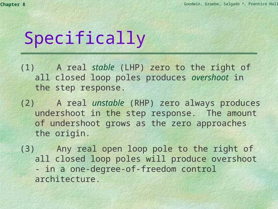
(1) A real stable (LHP) zero to the right of all closed loop poles produces overshoot in the step response.

(2) A real unstable (RHP) zero always produces undershoot in the step response. The amount of undershoot grows as the zero approaches the origin.

(3) Any real open loop pole to the right of all closed loop poles will produce overshoot - in a one-degree-of-freedom control architecture.


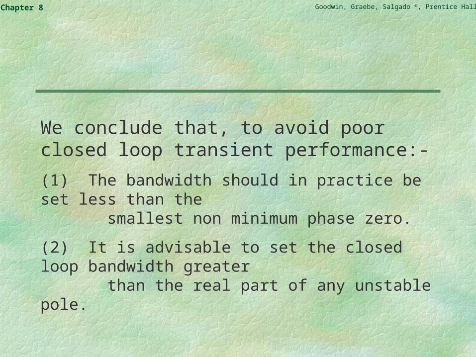
We conclude that, to avoid poor closed loop transient performance:-

(1) The bandwidth should in practice be set less than the smallest non minimum phase zero.

(2) It is advisable to set the closed loop bandwidth greater than the real part of any unstable pole.


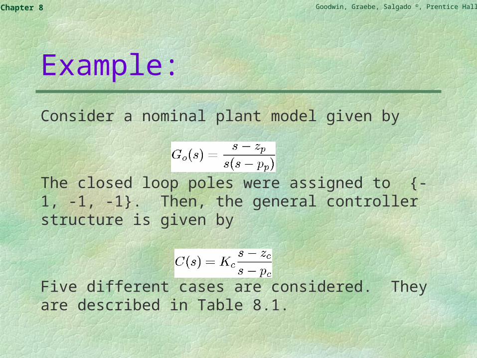
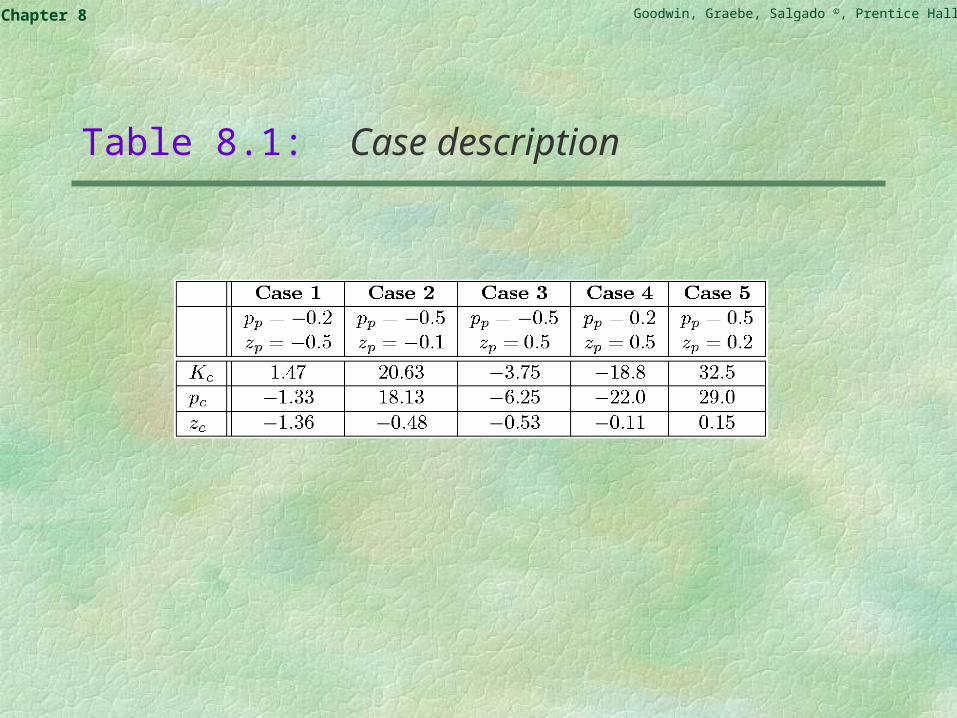
Example:

Consider a nominal plant model given by

The closed loop poles were assigned to {-1, -1, -1}. Then, the general controller structure is given by

Five different cases are considered. They are described in Table 8.1.


Table 8.1: Case description


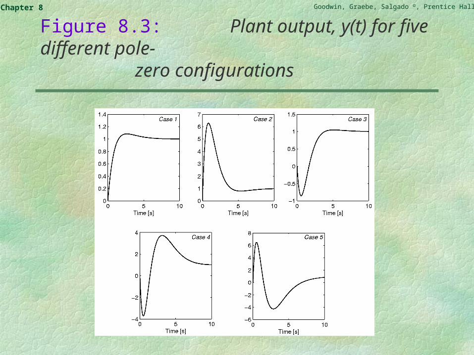
Figure 8.3: Plant output, y(t) for five different pole-zero configurations


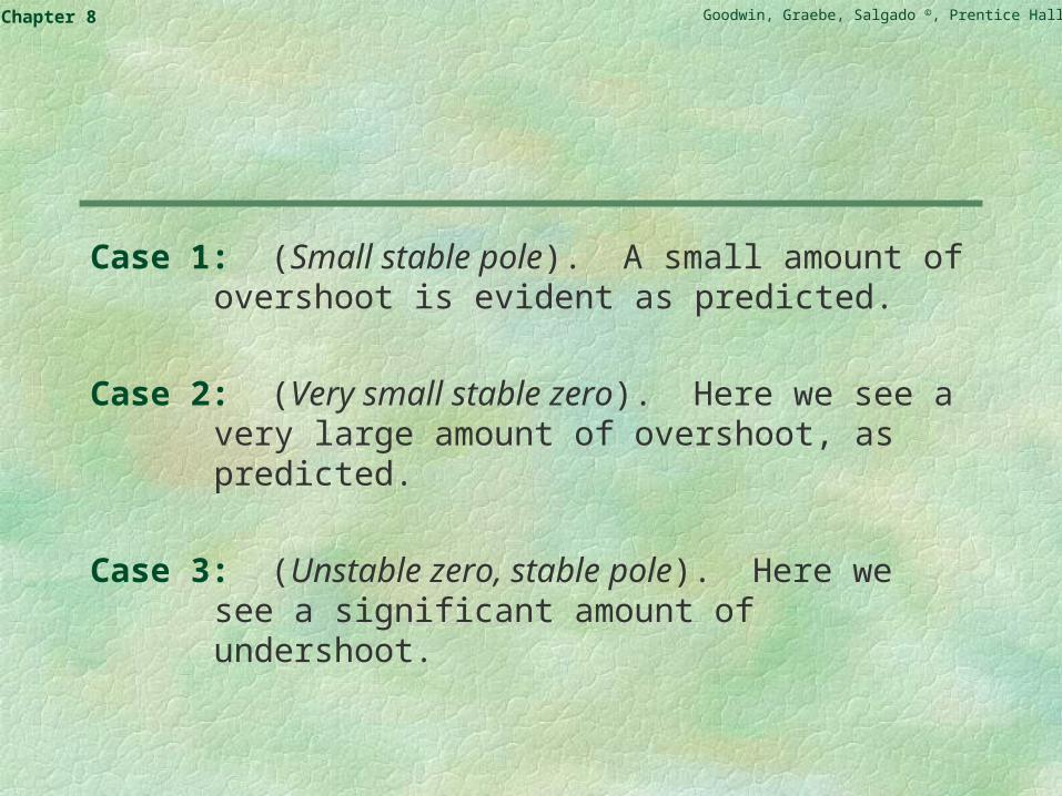
Case 1: (Small stable pole). A small amount of overshoot is evident as predicted.

Case 2: (Very small stable zero). Here we see a very large amount of overshoot, as predicted.

Case 3: (Unstable zero, stable pole). Here we see a significant amount of undershoot.


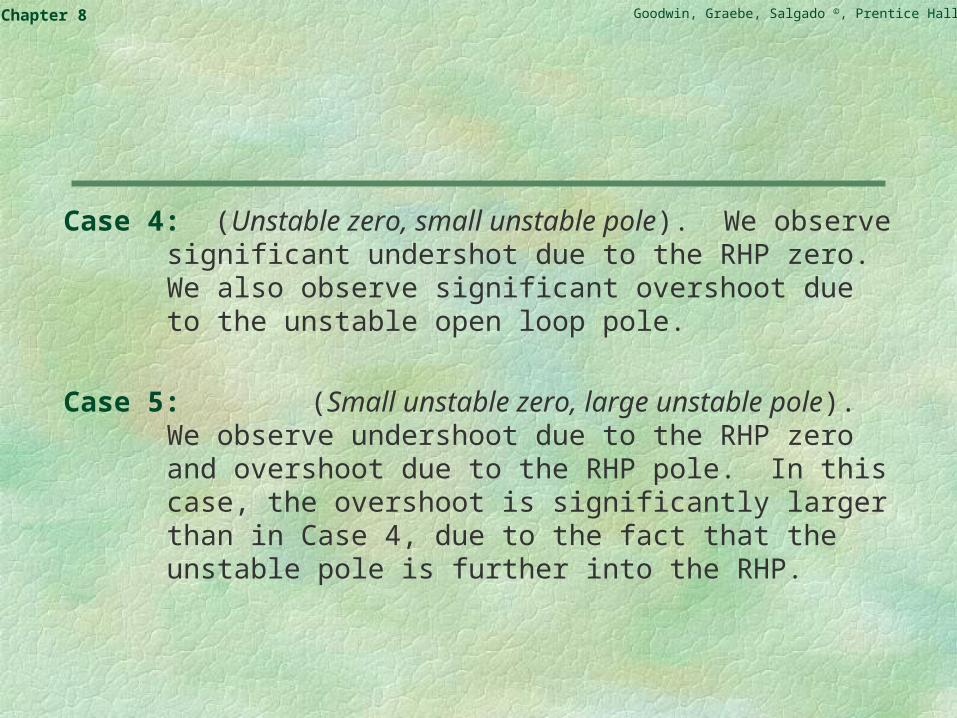
Case 4: (Unstable zero, small unstable pole). We observe significant undershot due to the RHP zero. We also observe significant overshoot due to the unstable open loop pole.

Case 5: (Small unstable zero, large unstable pole). We observe undershoot due to the RHP zero and overshoot due to the RHP pole. In this case, the overshoot is significantly larger than in Case 4, due to the fact that the unstable pole is further into the RHP.


Effect of Imaginary Axis Poles and Zeros

An interesting special case of Lemma 8.3 occurs when the plant has poles or zeros on the imaginary axis.


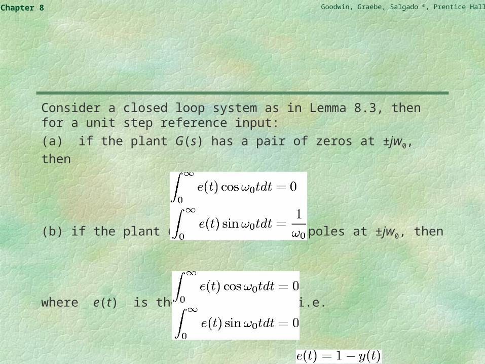
Consider a closed loop system as in Lemma 8.3, then for a unit step reference input:

(a) if the plant G(s) has a pair of zeros at ±jw0, then

(b) if the plant G(s) has a pair of poles at ±jw0, then

where e(t) is the control error, i.e.


We see from the above formula that the maximum error in the step response will be very large if one tries to make the closed loop bandwidth greater than the position of the resonant zeros.

We illustrate by a simple example:


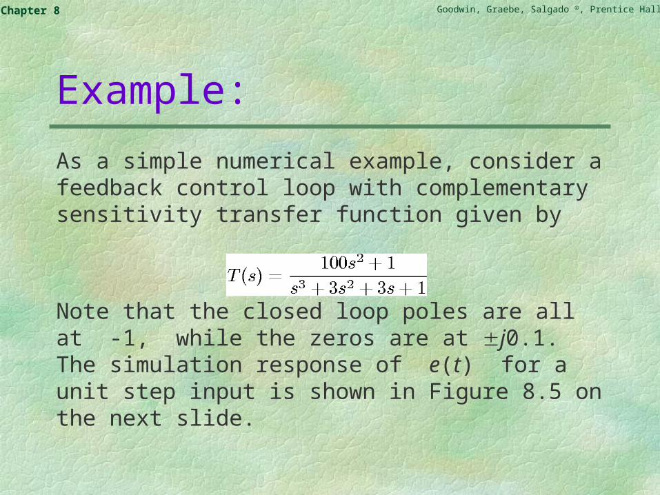
Example:

As a simple numerical example, consider a feedback control loop with complementary sensitivity transfer function given by

Note that the closed loop poles are all at -1, while the zeros are at j0.1. The simulation response of e(t) for a unit step input is shown in Figure 8.5 on the next slide.


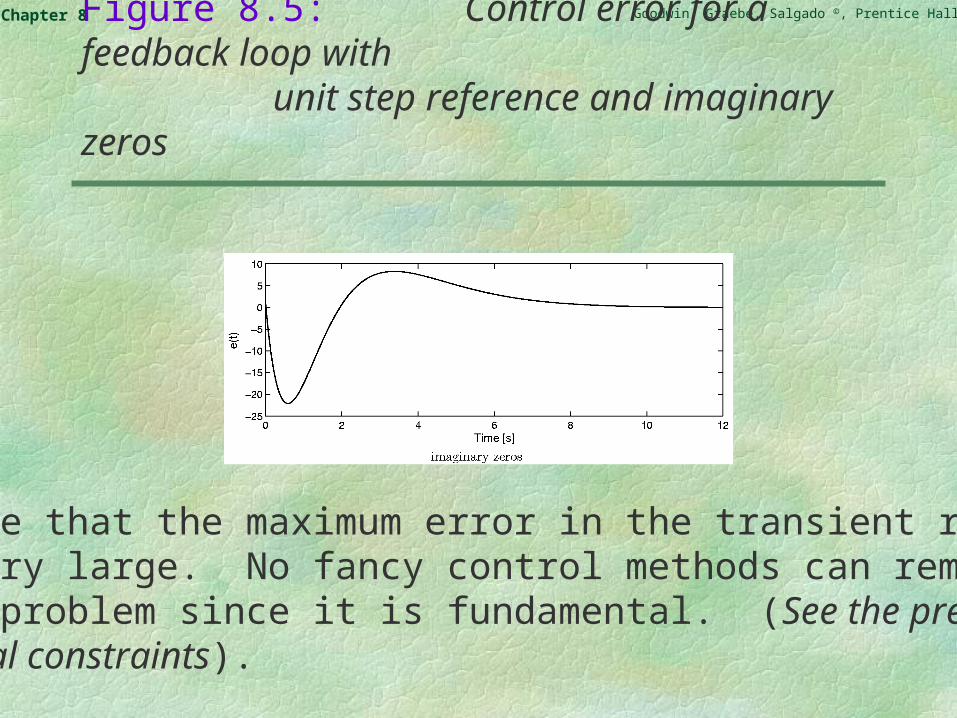
Figure 8.5: Control error for a feedback loop with unit step reference and imaginary zeros

We see that the maximum error in the transient responseis very large. No fancy control methods can remedythis problem since it is fundamental. (See the previousintegral constraints).


An Industrial Application (Hold-Up Effect in Reversing Mill)

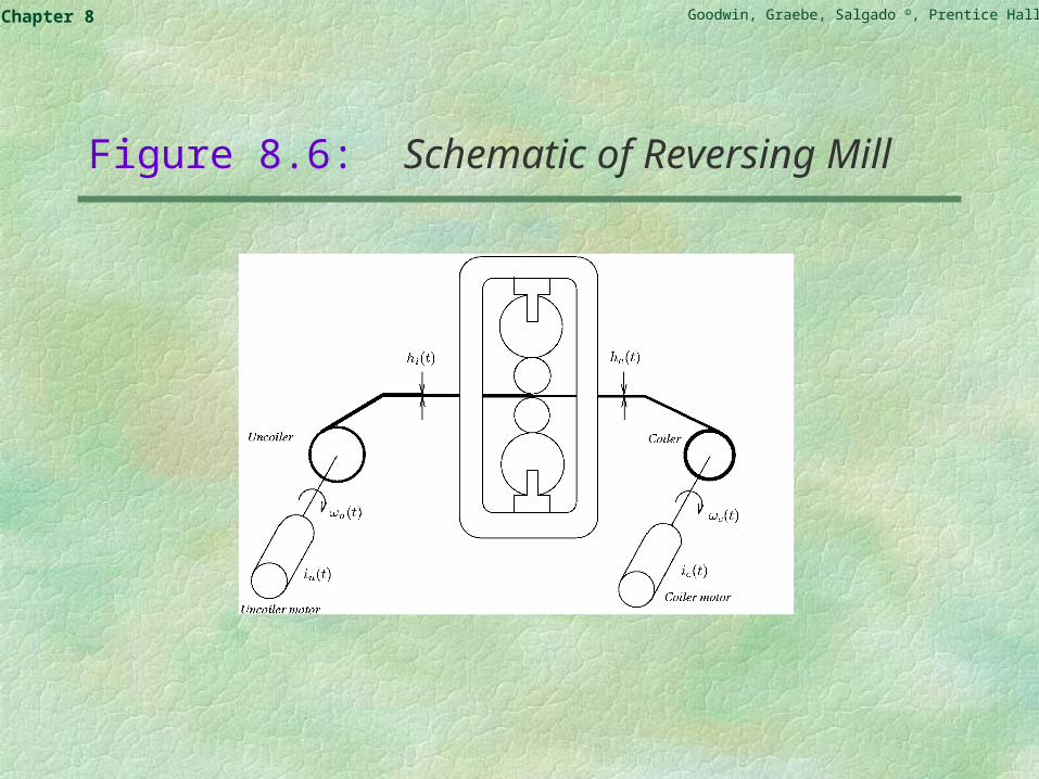
Here we study a reversing rolling mill. In this form of rolling mill the strip is successively passed from side to side so that the thickness is successfully reduced on each pass.

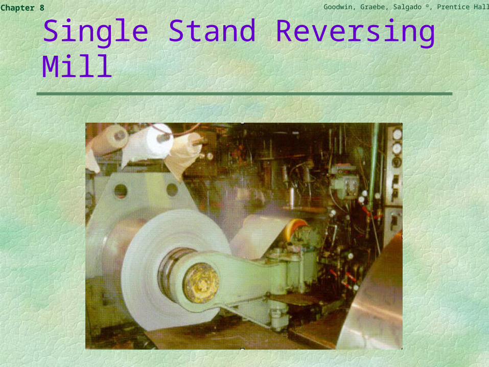
For a photo of a reversing mill see the next slide. For a schematic diagram of a single stand reversing rolling mill, see Figure 8.6.


Single Stand Reversing Mill


Figure 8.6: Schematic of Reversing Mill


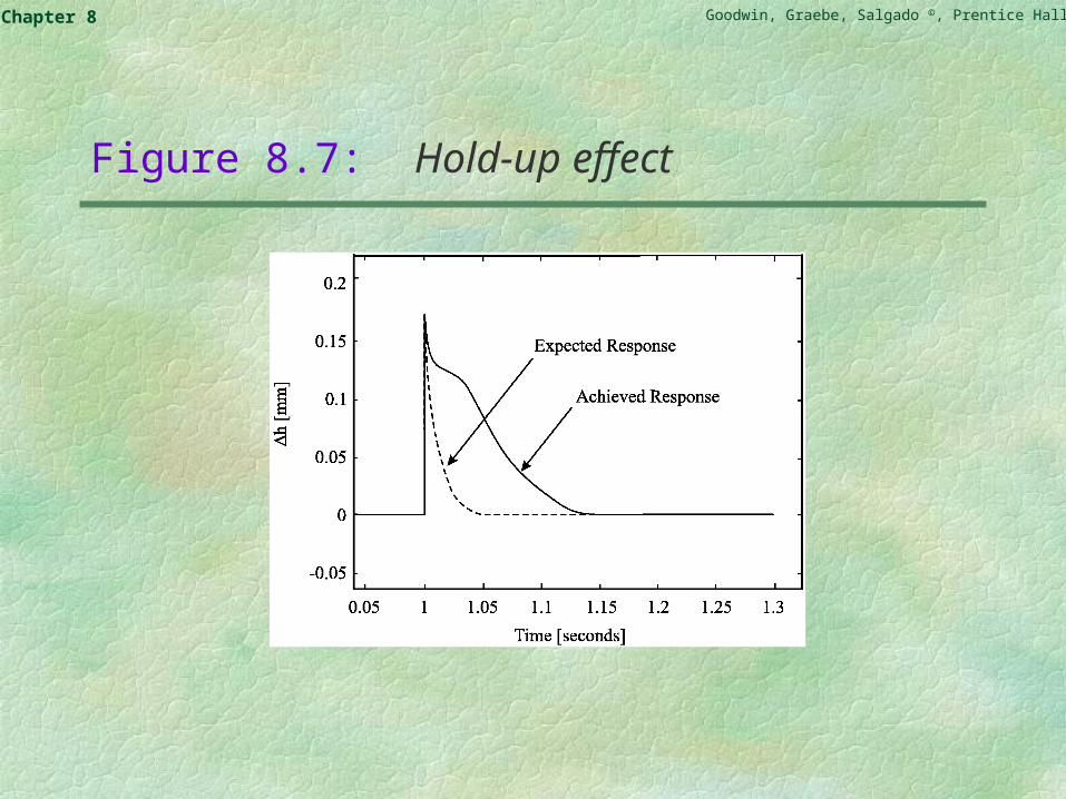
Despite great efforts to come up with a suitable design, the closed loop response of these systems tends to start out fast but then tends to hold-up. A typical response to a step input disturbance is shown schematically in Figure 8.7.


Figure 8.7: Hold-up effect


5.14

5.16

5.18

5.2

5.22

5.24

5.26

442.5 443 443.5 444 444.5 445 445.5

-4.5

-4

-3.5

-3

-2.5

-2

-1.5

-1

-0.5

Rol

lgap

in m

m

Time in seconds

Exit T

hic kn es s De vi ati on in m

m

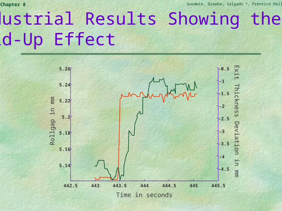
Industrial Results Showing the Hold-Up Effect


The reader may wonder:

1. How the above result occurs, and

2. How it can be remedied.

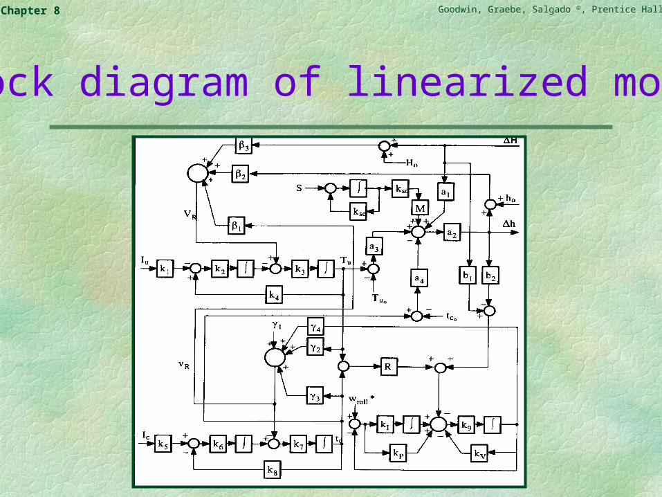
To answer this question, we build a model for the system. The associated Simulink diagram is shown on the next slide.


Block diagram of linearized model


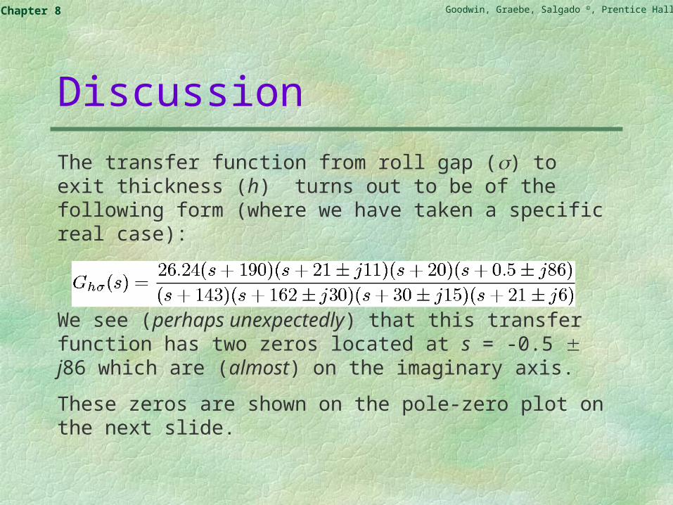
Discussion

The transfer function from roll gap () to exit thickness (h) turns out to be of the following form (where we have taken a specific real case):

We see (perhaps unexpectedly) that this transfer function has two zeros located at s = -0.5 j86 which are (almost) on the imaginary axis.

These zeros are shown on the pole-zero plot on the next slide.


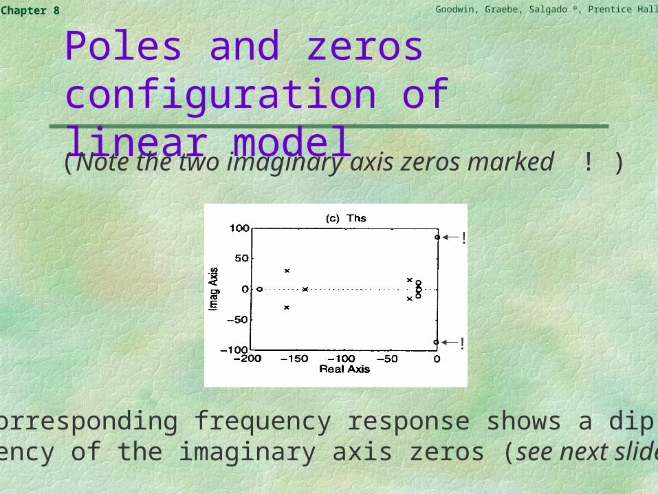
Poles and zeros configuration of linear model

!

!

(Note the two imaginary axis zeros marked ! )

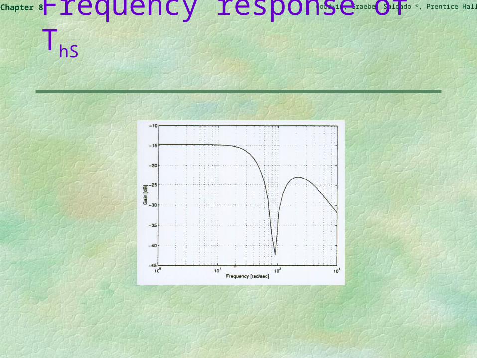
The corresponding frequency response shows a dip at thefrequency of the imaginary axis zeros (see next slide).


Frequency response of ThS


A physical explanation for the zeros is provided by thickness-tension interactions. This is described on the next slide.


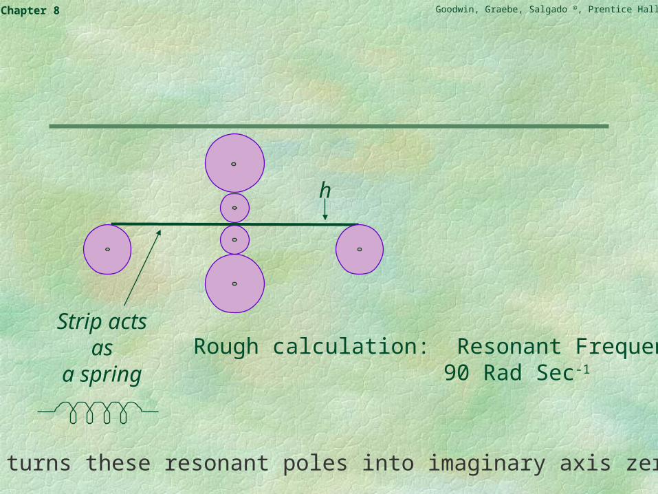
Strip actsas

a springRough calculation: Resonant Frequency

90 Rad Sec-1

h

Slip turns these resonant poles into imaginary axis zeros.


Next, recall the fundamental limitations arising from imaginary axis zeros. These are summarized on the next slide.


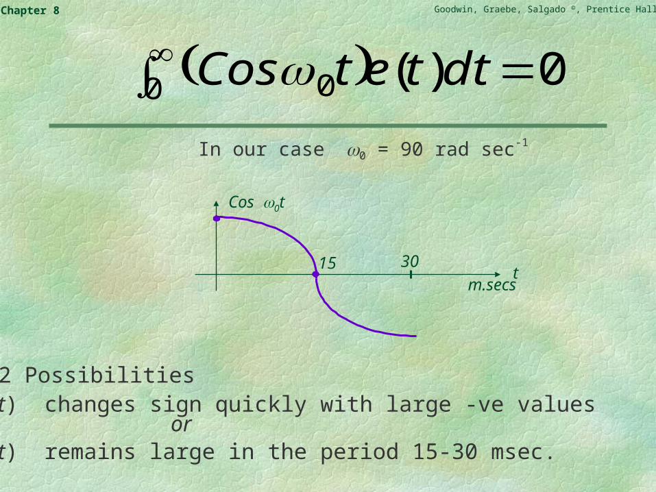
In our case 0 = 90 rad sec-1

0)(0 0 dttetCos

15 30t

m.secs

Cos 0t

Only 2 Possibilities e(t) changes sign quickly with large -ve values

or e(t) remains large in the period 15-30 msec.


Our previous analysis therefore suggests that the 2 (near) imaginary axis zeros will place fundamental limitations on the closed loop response time if significantly bad transients are to be avoided. Also, these limitations are fundamental, i.e. no fancy control system design can remedy the problem.


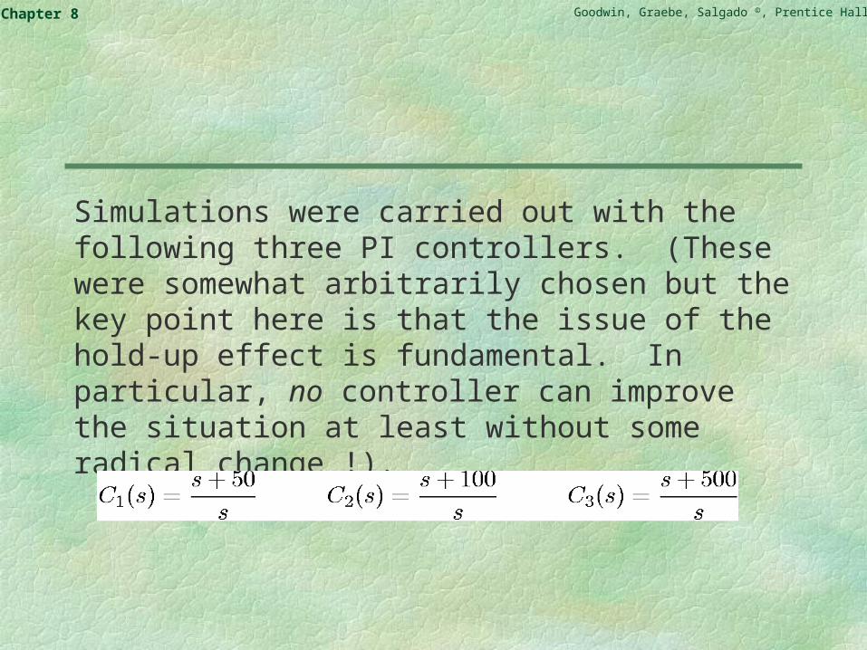
Simulations were carried out with the following three PI controllers. (These were somewhat arbitrarily chosen but the key point here is that the issue of the hold-up effect is fundamental. In particular, no controller can improve the situation at least without some radical change !).


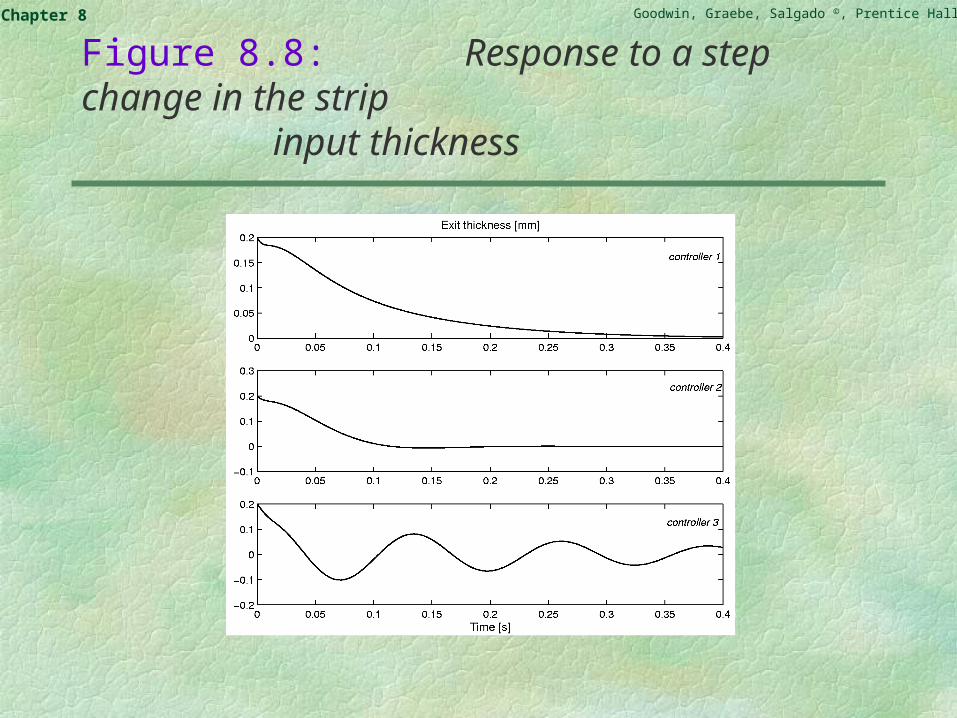
Figure 8.8: Response to a step change in the strip input thickness


Observations

We see that, as we attempt to increase the closed loop bandwidth (i.e. reduce the closed loop transient time) so the response deteriorates. This is in line with our previous predictions.


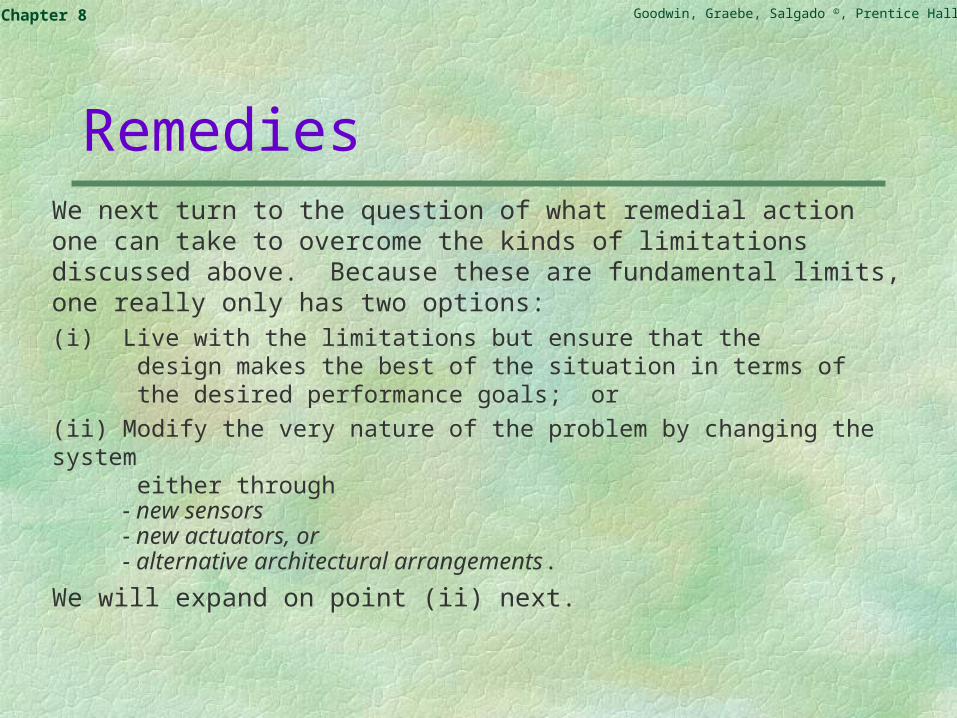
RemediesWe next turn to the question of what remedial action one can take to overcome the kinds of limitations discussed above. Because these are fundamental limits, one really only has two options:(i) Live with the limitations but ensure that the design makes the best of the situation in terms of the desired performance goals; or

(ii) Modify the very nature of the problem by changing the system either through

- new sensors- new actuators, or- alternative architectural arrangements.

We will expand on point (ii) next.


Alternative Sensors

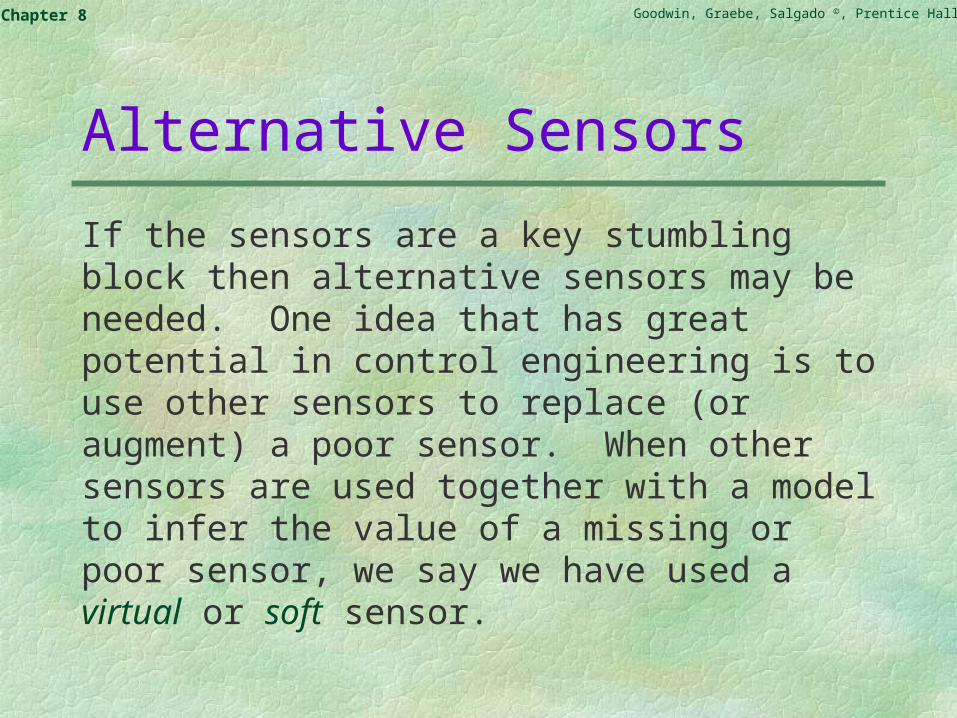
If the sensors are a key stumbling block then alternative sensors may be needed. One idea that has great potential in control engineering is to use other sensors to replace (or augment) a poor sensor. When other sensors are used together with a model to infer the value of a missing or poor sensor, we say we have used a virtual or soft sensor.


Thickness control in rolling mills revisited

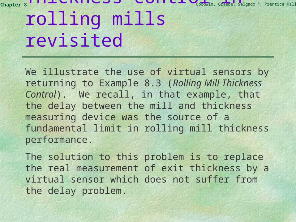
We illustrate the use of virtual sensors by returning to Example 8.3 (Rolling Mill Thickness Control). We recall, in that example, that the delay between the mill and thickness measuring device was the source of a fundamental limit in rolling mill thickness performance.

The solution to this problem is to replace the real measurement of exit thickness by a virtual sensor which does not suffer from the delay problem.


Development of Virtual Sensor

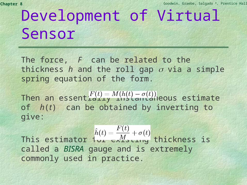
The force, F can be related to the thickness h and the roll gap via a simple spring equation of the form.

Then an essentially instantaneous estimate of h(t) can be obtained by inverting to give:

This estimator for existing thickness is called a BISRA gauge and is extremely commonly used in practice.


An alternative virtual sensor

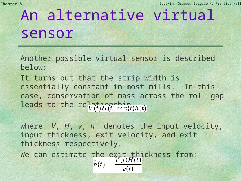
Another possible virtual sensor is described below:

It turns out that the strip width is essentially constant in most mills. In this case, conservation of mass across the roll gap leads to the relationship

where V, H, v, h denotes the input velocity, input thickness, exit velocity, and exit thickness respectively.

We can estimate the exit thickness from:


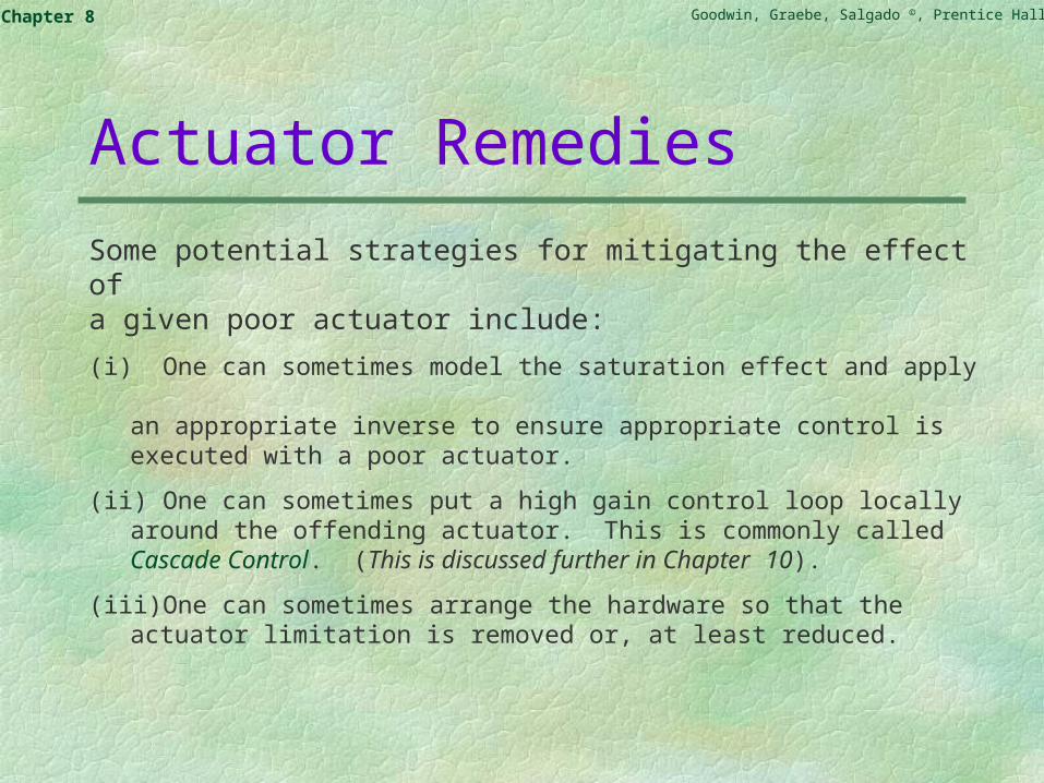
Actuator Remedies

Some potential strategies for mitigating the effect of a given poor actuator include:

(i) One can sometimes model the saturation effect and apply an appropriate inverse to ensure appropriate control is executed with a poor actuator.

(ii) One can sometimes put a high gain control loop locally around the offending actuator. This is commonly called Cascade Control. (This is discussed further in Chapter 10).

(iii) One can sometimes arrange the hardware so that the actuator limitation is removed or, at least reduced.


We study below a special way of arranging the control law to mitigate the bad effects of controller saturation.


Anti-Windup Mechanisms

When an actuator is limited in amplitude or slew rate, then one can often avoid the problem by reducing the performance demands. However, in other applications it is desirable to push the actuator hard up against the limits so as to gain the maximum benefit from the available actuator authority. This makes the best of the given situation. However, there is a down-side associated with this strategy.

In particular, one of the costs of driving an actuator into a maximal limit is associated with the problem of integral wind-up.


In particular, when the input is saturated the control is constant and hence the error cannot be reduced. Under these conditions, the I term in the PID controller will grow leading to poor transient/response. This is called wind-up.

For the moment it suffices to remark that the core idea used to protect systems against the negative effects of wind-up is to turn the integrator off whenever the input reaches a limit. This can either be done by a switch or by implementing the integrator in such a way that it automatically turns off when the input reaches a limit.


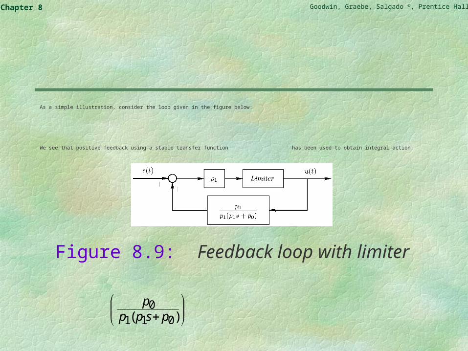
As a simple illustration, consider the loop given in the figure below:

We see that positive feedback using a stable transfer function has been used to obtain integral action.

Figure 8.9: Feedback loop with limiter

)( 0110

psppp


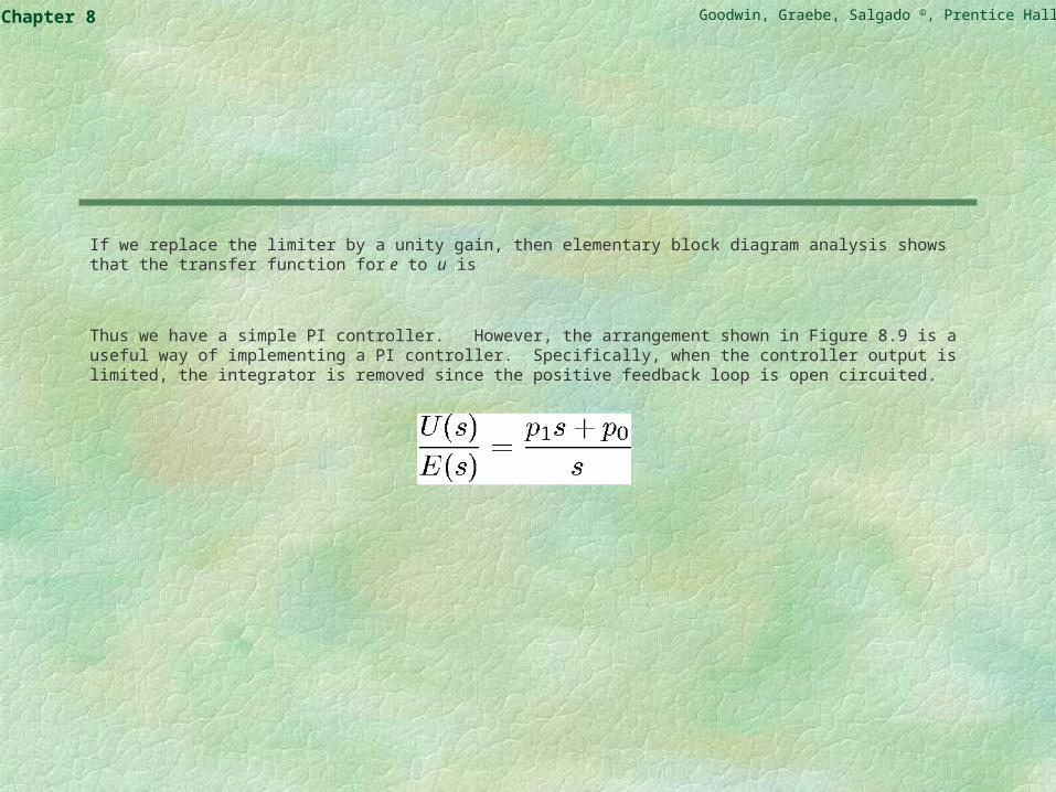
If we replace the limiter by a unity gain, then elementary block diagram analysis shows that the transfer function for e to u is

Thus we have a simple PI controller. However, the arrangement shown in Figure 8.9 is a useful way of implementing a PI controller. Specifically, when the controller output is limited, the integrator is removed since the positive feedback loop is open circuited.


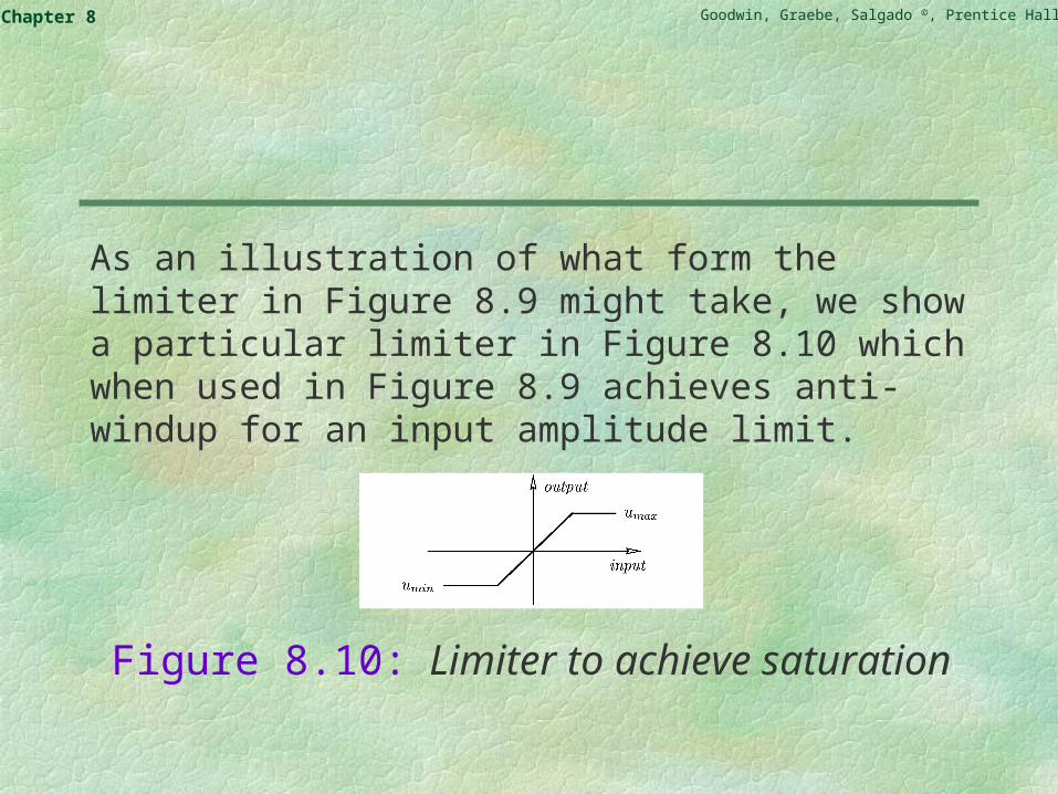
As an illustration of what form the limiter in Figure 8.9 might take, we show a particular limiter in Figure 8.10 which when used in Figure 8.9 achieves anti-windup for an input amplitude limit.

Figure 8.10: Limiter to achieve saturation


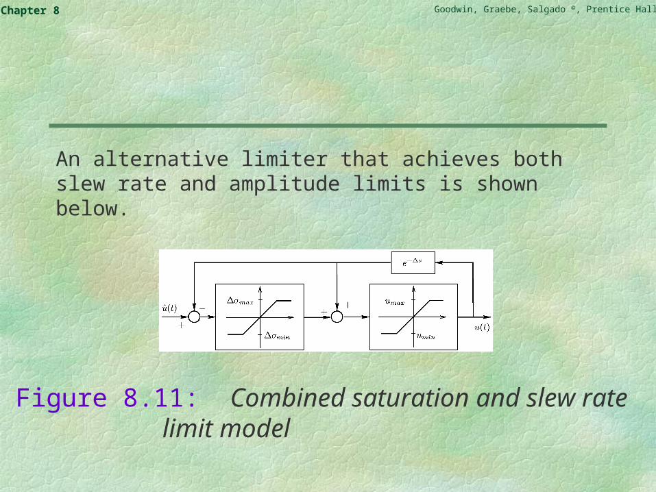
An alternative limiter that achieves both slew rate and amplitude limits is shown below.

Figure 8.11: Combined saturation and slew rate limit model


We will discuss the above kind of anti-windup protection in much greater detail in:

Chapter 11 (Dealing with Constraints)

and

Chapter 23 (Model Predictive Control).


Remedies for Minimal Actuation Movement

Minimal actuator movements are difficult to remedy. In some applications, it is possible to use dual-range controllers wherein a large actuator is used to determine the majority of the control force but a smaller actuator is used to give a fine-trim.

An example of this is given on the book’s web page in relation to pH Control.

In other applications we must live with the existing actuator.


Continuous Caster RevisitedWe recall the sustained oscillation problem due to actuator minimal movements described in Example 8.2.

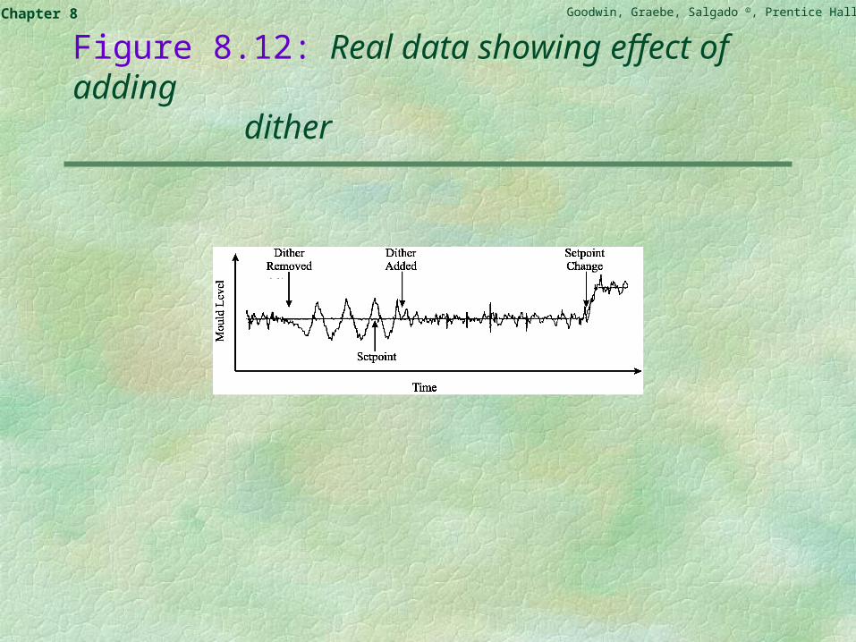
One cannot use dual-range control in this application because a small-high-precision valve would immediately clog with solidified steel. A solution we have used to considerable effect in this application is to add a small high frequency dither signal to the valve. This keeps the valve in motion and hence minimizes stiction effects. The high frequency input dither is filtered out by the dynamics of the process and thus does not have a significant impact on the final product quality. Of course, one does pay the price of having extra wear on the valve due to the presence of the dither signal. However, this cost is off-set by the very substantial improvements in product quality as seen at the output. Some real data is shown in Figure 8.12.


Figure 8.12: Real data showing effect of adding dither


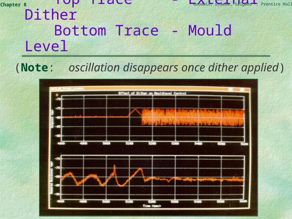
Further Real Data: Top Trace - External DitherBottom Trace - Mould Level

(Note: oscillation disappears once dither applied)


Finally, we turn to the impact of the process itself. We have discussed these limitations under the headings of:

delaysopen loop plant polesopen loop plant zeros

The limitations arising from these effects are fundamental WITHIN THE GIVEN ARCHITECTURE ! This suggests that the one to overcome these limitations is to consider changing the basic architecture of the problem.


Architectural Changes

The fundamental limits we have described apply to the given set-up. Clearly, if one changes the physical system in some way then the situation changes. Indeed, these kinds of change are a very powerful tool in the hands of the control system designer.


The above idea will actually be a central theme as we move forward in these notes. Indeed, we will give many industrial examples of the power of architectural changes. For example, in Chapter 10 we will show how feedforward and cascade loops can dramatically improve performance. We will also see how a simple architectural change can resolve the fundamental problem of the hold-up effect in Rolling Mills (see earlier in this chapter).


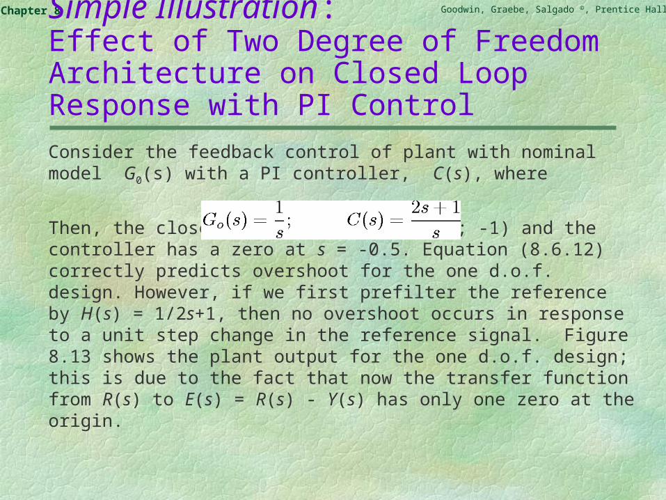
Simple Illustration: Effect of Two Degree of Freedom Architecture on Closed Loop Response with PI Control

Consider the feedback control of plant with nominal model G0(s) with a PI controller, C(s), where

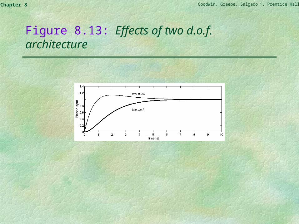
Then, the closed loop poles are at (-1; -1) and the controller has a zero at s = -0.5. Equation (8.6.12) correctly predicts overshoot for the one d.o.f. design. However, if we first prefilter the reference by H(s) = 1/2s+1, then no overshoot occurs in response to a unit step change in the reference signal. Figure 8.13 shows the plant output for the one d.o.f. design; this is due to the fact that now the transfer function from R(s) to E(s) = R(s) - Y(s) has only one zero at the origin.


Figure 8.13: Effects of two d.o.f. architecture


Design Homogeneity Revisited

We have seen above that limitations arise from different effects. For example, the following factors typically place an upper limit on the usable bandwidth

Actuator slew rate and amplitude limits Model error Delays Right half plane or imaginary axis zeros

This leads to the obvious question: which of these limits, if any, do I need to consider? The answer is that it is clearly best to focus on that particular issue which has the most impact.


This is because the greatest return comes from influencing the most significant factor.

Indeed, in an ideal situation, the final errors due to various sources should all be comparable (otherwise the possibility exists that one has over expended effort in reducing one source of error when it wasn’t dominant). We call this design homogeneity.


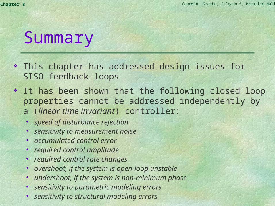
Summary

This chapter has addressed design issues for SISO feedback loops

It has been shown that the following closed loop properties cannot be addressed independently by a (linear time invariant) controller:

speed of disturbance rejection sensitivity to measurement noise accumulated control error required control amplitude required control rate changes overshoot, if the system is open-loop unstable undershoot, if the system is non-minimum phase sensitivity to parametric modeling errors sensitivity to structural modeling errors


Rather, tuning for one of these properties automatically impacts on the others.

For example, irrespectively of how a controller is synthesized and tuned, if the effect of the measurement noise on the output is T0(s), then the impact of an output disturbance is necessarily 1 - T0(s). Thus, any particular frequency cannot be removed from both an output disturbance and the measurement noise as one would require T0(s) to be close to 0 at that frequency, whereas the other would require T0(s) to be close to 1. One can therefore only reject one at the expense of the other, or compromise.


Thus, a faster rejection of disturbances, is generally associated with

higher sensitivity to measurement noise less control error larger amplitude and slew rates in the control action higher sensitivity to structural modeling errors more undershoot, if the system is non-minimum phase less overshoot if the system is unstable.


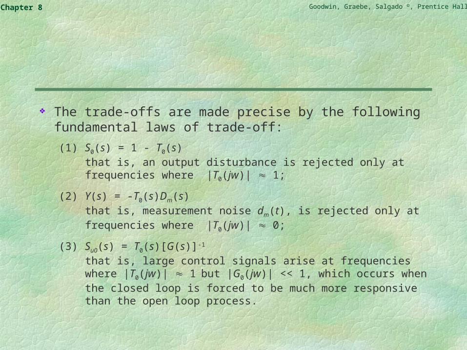
The trade-offs are made precise by the following fundamental laws of trade-off:

(1) S0(s) = 1 - T0(s)that is, an output disturbance is rejected only at frequencies where |T0(jw)| 1;

(2) Y(s) = -T0(s)Dm(s)that is, measurement noise dm(t), is rejected only at frequencies where |T0(jw)| 0;

(3) Su0(s) = T0(s)[G(s)]-1

that is, large control signals arise at frequencies where |T0(jw)| 1 but |G0(jw)| << 1, which occurs when the closed loop is forced to be much more responsive than the open loop process.


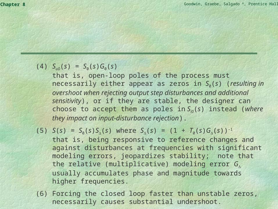
(4) Su0(s) = S0(s)G0(s)that is, open-loop poles of the process must necessarily either appear as zeros in S0(s) (resulting in overshoot when rejecting output step disturbances and additional sensitivity), or if they are stable, the designer can choose to accept them as poles in Si0(s) instead (where they impact on input-disturbance rejection).

(5) S(s) = S0(s)S(s) where S(s) = (1 + T0(s)G(s))-1

that is, being responsive to reference changes and against disturbances at frequencies with significant modeling errors, jeopardizes stability; note that the relative (multiplicative) modeling error G usually accumulates phase and magnitude towards higher frequencies.

(6) Forcing the closed loop faster than unstable zeros, necessarily causes substantial undershoot.


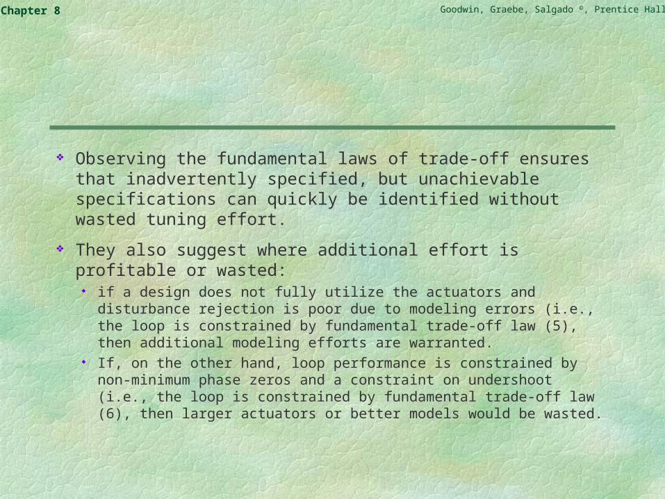
Observing the fundamental laws of trade-off ensures that inadvertently specified, but unachievable specifications can quickly be identified without wasted tuning effort.

They also suggest where additional effort is profitable or wasted:

if a design does not fully utilize the actuators and disturbance rejection is poor due to modeling errors (i.e., the loop is constrained by fundamental trade-off law (5), then additional modeling efforts are warranted.

If, on the other hand, loop performance is constrained by non-minimum phase zeros and a constraint on undershoot (i.e., the loop is constrained by fundamental trade-off law (6), then larger actuators or better models would be wasted.


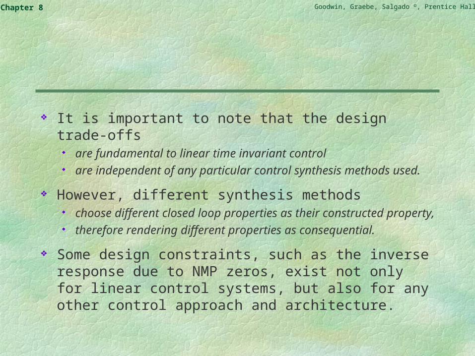
It is important to note that the design trade-offs are fundamental to linear time invariant control are independent of any particular control synthesis methods used.

However, different synthesis methods choose different closed loop properties as their constructed

property, therefore rendering different properties as consequential.

Some design constraints, such as the inverse response due to NMP zeros, exist not only for linear control systems, but also for any other control approach and architecture.


Remedies for the fundamental limits do exist but they inevitably require radical changes, e.g.

seeking alternative senses seeking alternative actuators modifying the basic architecture of the plant or controller.


We have seen that: sensors are the eyes of control. Consequently, if the sensors are poor

then good performance cannot be achieved.

Actuators provide the muscles for control; i.e. the motive force to move from where the plant states are to where we want then to be. Consequently if actuators are poor then good performance cannot be achieved.

However, good eyes and strong muscles are not enough for high performance control. The reader is encouraged to think of somebody they know who has good eyesight and who is strong but who cannot play a competitive sport at A-grade level. Of course, the extra ingredient is hand-eye coordination, I.e. the connection between sensors and actuators.


This connection has many difficult aspects. For example, if one thinks about playing tennis well, then one realizes that it is much more than hitting the ball hard. One needs to

predict where the ball will go; predict where the opponent will run; sometimes put spin or lob the ball.

These things take a long time to learn to do well, i.e. designing a high performance feedback controller connecting sensors to actuators is a non-trivial task. This is the subject of this book. We remind the reader of the following slide (from Chapter 1) which captures the above ideas in cartoon form:


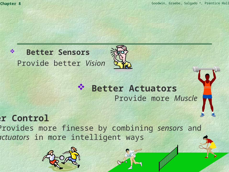
Better ControlProvides more finesse by combining sensors and actuators in more intelligent ways

Better ActuatorsProvide more Muscle

Better Sensors

Provide better Vision

Documents

Goodwin, Graebe, Salgado ©, Prentice Hall 2000 Chapter 8 Fundamental Design Limitations in SISO Control