Goodness of Fit: What Do We Really Want to Know?I. NarskyCalifornia Institute of Technology, Pasadena, CA 91125, USA

Definitions of the goodness-of-fit problem are discussed. A new method for estimation of the goodness of fitusing distance to nearest neighbor is described. Performance of several goodness-of-fit methods is studied fortime-dependent CP asymmetry measurements of sin(2β).

1. INTRODUCTION

The goodness-of-fit problem has recently attractedattention from the particle physics community. Inmodern particle experiments, one often performs anunbinned likelihood fit to data. The experimenterthen needs to estimate how accurately the fit functionapproximates the observed distribution. A number ofmethods have been used to solve this problem in thepast [1], and a number of methods have been recentlyproposed [2, 3] in the physics literature.

For binned data, one typically applies a χ2 statisticto estimate the fit quality. Without discussing advan-tages and flaws of this approach, I would like to stressthat the application of the χ2 statistic is limited. Theχ2 test is neither capable nor expected to detect fitinefficiencies for all possible problems. This is a pow-erful and versatile tool but it should not be consideredas the ultimate solution to every goodness-of-fit prob-lem.

There is no such popular method, an equivalent ofthe χ2 test, for unbinned data. The maximum like-lihood value (MLV) test has been frequently used inpractice but it often fails to provide a reasonable an-swer to the question at hand: how well are the datamodelled by a certain density [4]? It is only naturalthat goodness-of-fit tests for small data samples areharder to design and less versatile than those for largesamples. For small data samples, asymptotic approx-imations do not hold and the performance of everygoodness-of-fit test needs to be studied carefully onrealistic examples. Thus, the hope for a versatile un-binned goodness-of-fit procedure expressed by somepeople at the conference seems somewhat naive.

A more important practical question is how to de-sign a powerful goodness-of-fit test for each individualproblem. It is not possible to answer this question un-less we specify in more narrow terms the problem thatwe are trying to solve.

2. WHAT IS A GOODNESS-OF-FIT TEST?

A hypothesis test requires formulation of null andalternative hypotheses. The confidence level, 1 − αI ,

of the test is then defined as the probability of ac-cepting the null hypothesis given it is true, and thepower of the test, 1 − αII , is defined as the probabil-ity of rejecting the null hypothesis given the alterna-tive is true. Above, αI and αII denote Type I andType II errors, respectively. An ideal hypothesis testis uniformly most powerful (UMP) because it givesthe highest power among all possible tests at the fixedconfidence level. In most realistic problems, it is notpossible to find a UMP test and one has to considervarious tests with acceptable power functions.

There is a long-standing controversy about the con-nection between hypothesis testing and the goodness-of-fit problem. It can be argued [5] that there can beno alternative hypothesis for the goodness-of-fit test.In this approach, however, the experimenter does nothave any criteria for choosing one goodness-of-fit pro-cedure over another. One can design a goodness-of-fit test using first principles, advanced computationalmethods, rich intuition or black magic. But the prac-titioner wants to know how well this method will per-form in specific situations. To evaluate this perfor-mance, one needs to study the power of the proposedmethod against a few specific alternatives. A certain,perhaps vague, notion of an alternative hypothesismust be adopted for this exercise; hence, a certain,perhaps vague, notion of the alternative hypothesis istypically used to design a goodness-of-fit test.

Consider, for example, testing uniformity on an in-terval. The alternative is usually perceived as pres-ence of peaks in the data. Suppose we design a pro-cedure that gives the highest goodness-of-fit value forequidistant experimental points. This test will per-form well for the chosen alternative. In reality, how-ever, we may need to test exponentiality of the pro-cess. For instance, we use a Geiger counter to measureelapsed time between two consecutive events and plotthese time intervals next to each other on a straightline. In this case, equidistant data would imply thatthe process is not as random as we thought, and thedesigned goodness-of-fit procedure would fail to detectthe inconsistency between the data and the model.Tests against highly structured data (e.g., equidistantone-dimensional data) have been, in fact, a subject ofstatistical research on goodness-of-fit methods.

The question therefore is how to state the alterna-tive hypothesis in a way appropriate for each individ-

PHYSTAT2003, SLAC, Stanford, California, September 8-11, 2003

70

ual problem. I emphasize that I am not suggesting touse a directional test for one specific well-defined alter-native. The goal is to design an omnibus goodness-of-fit test that discriminates against at least severalplausible alternatives.

The null hypothesis is defined as

H0 : X ∼ f(x|θ0, η) , (1)

where X is a multivariate random variable, and f isthe fit density with a vector of arguments x, vectorof parameters θ and vector of nuisance parameters η.The alternative hypothesis is stated in the most gen-eral way as

H1 : X ∼ g(x) with g(x) 6= f(x|θ0, η) . (2)

A specific subclass of this alternative hypothesis thatis sometimes of interest is expressed as

H1 : X ∼ f(x|θ, η) with θ 6= θ0 . (3)

In other words, most usually we would like to testthe fit function against different shapes (2). For thetest (3), we assume that the shape of the fit functionis correctly modelled and we only need to cross-checkthe value of the parameter.

If a statistic S(x) is used to judge the fit quality,the goodness-of-fit is given by

1 − αI =

∫

fS(s)>fS(s0)

fS(s)ds , (4)

where s0 is the value of the statistic observed in theexperiment, and fS(s) is the distribution of the statis-tic under the null hypothesis.

In practice, the vector of parameter estimates θ0 isusually extracted from an unbinned maximum likeli-

hood (ML) fit to the data: θ0 = θ(x). In this case, thegoodness-of-fit statistic must be independent of, or atmost weakly correlated to, the ML estimator of the

parameter: ρ(S(x), θ(x)) ≈ 0, where ρ is the corre-lation coefficient computed under the null hypothesis.

If S(x) and θ(x) are strongly correlated, the goodness-of-fit test is redundant.

The ML estimator itself is usually a powerful toolfor discrimination against the alternative (3). In this

case, the statistic S(x) 6= θ(x) can be treated as anindependent cross-check of the parameters θ0.

The nuisance parameters η should affect our judg-ment about the fit quality as little possible. Discus-sion of methods for handling nuisance parameters isbeyond the scope of this note.

3. DISTANCE TO NEAREST NEIGHBORTEST

The idea of using Euclidian distance between near-est observed experimental points as a goodness-of-fitmeasure is not new. Clark and Evans [6] used an av-erage distance between nearest neighbors to test two-dimensional populations of various plants for unifor-mity. Later they extended this formalism to a highernumber of dimensions. Diggle [7] proposed to usean entire distribution of ordered distances to nearestneighbors and apply Kolmogorov-Smirnov or Cramer-von Mises tests to evaluate consistency between ex-perimentally observed and expected densities. Rip-ley [8] introduced a function, K(t), which representsa number of points within distance t of an arbitrarypoint of the process; he used the maximal deviationbetween expected and observed K(t) as a goodness-of-fit measure. Bickel and Breiman [9] introduced agoodness-of-fit test based on the distribution of thevariable exp (−Nf(xi)V (xi)), where f(xi) is the ex-pected density at the observed point xi, V (xi) is thevolume of a nearest neighbor sphere centered at xi

and N is the total number of observed points. An ap-proach closely related to distance-to-nearest-neighbortests is two-sample comparison based on counts ofnearest neighbors that belong to the same sample [10].These methods received substantial attention from thescience community and have been applied to numer-ous practical problems, mostly in ecology and medi-cal research. Ref. [11] offers a survey of distance-to-nearest-neighbor methods.

The goodness-of-fit test [3] uses a bivariate distribu-tion of the minimal and maximal distances to nearestneighbors. First, one transforms the fit function de-fined in an n-dimensional space of observables to auniform density in an n-dimensional unit cube. Thenone finds smallest and largest clusters of nearest neigh-bors whose linear size maximally deviates from theaverage cluster size predicted from uniformity. Thecluster size is defined as an average distance from thecentral point of the cluster to m nearest neighbors.If the experimenter has no prior knowledge of theoptimal number m of nearest neighbors included inthe goodness-of-fit estimation, one can try all possi-ble clusters 2 ≤ m ≤ N , where N is the total numberof observed experimental points. The probability ofobserving the smallest and largest clusters of this sizegives an estimate of the goodness of fit and the loca-tions of the clusters can be used to point out potentialproblems with data modelling.

This method is a good choice for detection of well-localized irregularities, e.g., unusual peaks in the data.Consider, for example, fitting a normal peak on top ofthe smooth background, as shown in Fig. 3. The like-lihood function is sensitive to the mean and width ofthe normal component. Hence, if the experimenter ismostly interested in how accurately these parameters

PHYSTAT2003, SLAC, Stanford, California, September 8-11, 2003

71

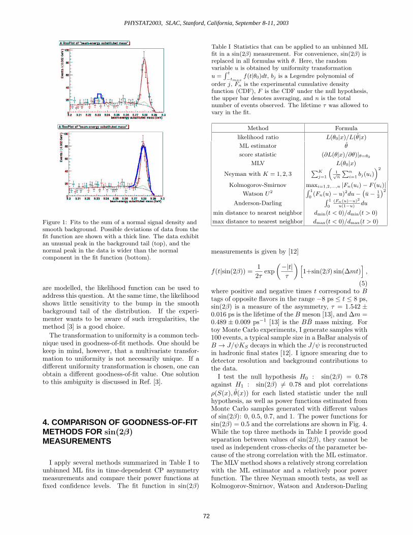
Figure 1: Fits to the sum of a normal signal density and

smooth background. Possible deviations of data from the

fit function are shown with a thick line. The data exhibit

an unusual peak in the background tail (top), and the

normal peak in the data is wider than the normal

component in the fit function (bottom).

are modelled, the likelihood function can be used toaddress this question. At the same time, the likelihoodshows little sensitivity to the bump in the smoothbackground tail of the distribution. If the experi-menter wants to be aware of such irregularities, themethod [3] is a good choice.

The transformation to uniformity is a common tech-nique used in goodness-of-fit methods. One should bekeep in mind, however, that a multivariate transfor-mation to uniformity is not necessarily unique. If adifferent uniformity transformation is chosen, one canobtain a different goodness-of-fit value. One solutionto this ambiguity is discussed in Ref. [3].

4. COMPARISON OF GOODNESS-OF-FITMETHODS FOR sin(2β)MEASUREMENTS

I apply several methods summarized in Table I tounbinned ML fits in time-dependent CP asymmetrymeasurements and compare their power functions atfixed confidence levels. The fit function in sin(2β)

Table I Statistics that can be applied to an unbinned ML

fit in a sin(2β) measurement. For convenience, sin(2β) is

replaced in all formulas with θ. Here, the random

variable u is obtained by uniformity transformation

u =∫

t

−tmax

f(t|θ0)dt, bj is a Legendre polynomial of

order j, Fn is the experimental cumulative density

function (CDF), F is the CDF under the null hypothesis,

the upper bar denotes averaging, and n is the total

number of events observed. The lifetime τ was allowed to

vary in the fit.

Method Formula

likelihood ratio L(θ0|x)/L(θ|x)

ML estimator θ

score statistic (∂L(θ|x)/∂θ)|θ=θ0

MLV L(θ0|x)

Neyman with K = 1, 2, 3∑

K

j=1

(

1√

n

∑

n

i=1bj(ui)

)2

Kolmogorov-Smirnov maxi=1,2,...,n |Fn(ui) − F (ui)|

Watson U2

∫

1

0(Fn(u) − u)2du −

(

u −1

2

)2

Anderson-Darling∫

1

0

(Fn(u)−u)2

u(1−u)du

min distance to nearest neighbor dmin(t < 0)/dmin(t > 0)

max distance to nearest neighbor dmax(t < 0)/dmax(t > 0)

measurements is given by [12]

f(t|sin(2β)) =1

2τexp

(

−|t|

τ

)

[

1+sin(2β) sin(∆mt)]

,

(5)where positive and negative times t correspond to Btags of opposite flavors in the range −8 ps ≤ t ≤ 8 ps,sin(2β) is a measure of the asymmetry, τ = 1.542 ±

0.016 ps is the lifetime of the B meson [13], and ∆m =0.489 ± 0.009 ps−1 [13] is the BB mass mixing. Fortoy Monte Carlo experiments, I generate samples with100 events, a typical sample size in a BaBar analysis ofB → J/ψKS decays in which the J/ψ is reconstructedin hadronic final states [12]. I ignore smearing due todetector resolution and background contributions tothe data.

I test the null hypothesis H0 : sin(2β) = 0.78against H1 : sin(2β) 6= 0.78 and plot correlations

ρ(S(x), θ(x)) for each listed statistic under the nullhypothesis, as well as power functions estimated fromMonte Carlo samples generated with different valuesof sin(2β): 0, 0.5, 0.7, and 1. The power functions forsin(2β) = 0.5 and the correlations are shown in Fig. 4.While the top three methods in Table I provide goodseparation between values of sin(2β), they cannot beused as independent cross-checks of the parameter be-cause of the strong correlation with the ML estimator.The MLV method shows a relatively strong correlationwith the ML estimator and a relatively poor powerfunction. The three Neyman smooth tests, as well asKolmogorov-Smirnov, Watson and Anderson-Darling

PHYSTAT2003, SLAC, Stanford, California, September 8-11, 2003

72

Figure 2: Correlations between the ML estimator of

sin(2β) and the chosen statistic (top). Power functions of

the hypothesis test H0 : sin(2β) = 0.78 against

H1 : sin(2β) 6= 0.78 versus confidence level (bottom) at

sin(2β) = 0.5.

tests, show small correlation to the ML estimator anddecent power functions; these tests perform compet-itively among each other. Yet Kolmogorov-Smirnovand Anderson-Darling tests produce somewhat bettercombinations of the small correlation and large powerfunction and should be preferred over others. Thedistance-to-nearest-neighbor test was designed for de-tection of well-localized regularities and hence was notexpected to give a high power function for the hypoth-esis test discussed here.

This exercise alone is insufficient to conclude thatthe two recommended tests are in fact the best om-nibus tests for fits of sin(2β). One would have to ex-tend this study to include other alternative densities,e.g., specific background shapes, that can distort theexperimental data.

5. SUMMARY

An acceptable goodness-of-fit test is defined as anomnibus test that discriminates against at least sev-

eral plausible alternatives. Numerous distance-to-nearest-neighbor methods for goodness-of-fit estima-tion have been described in the statistics literatureand should be tested in HEP practice. The distance-to-nearest-neighbor test based on minimal and max-imal distances should be used for detection of well-localized irregularities in the data. Correlation coef-ficients and power functions for several statistics arecompared for fits of sin(2β) in CP asymmetry mea-surements for one specific alternative.

Acknowledgments

I wish to thank the organizing committee of PHYS-TAT2003 for their effort. Thanks to Bob Cousins foruseful comments on this note.

Work partially supported by Department of Energyunder Grant DE-FG03-92-ER40701.

References

[1] R. D’Agostino and M. Stephens, “Goodness-of-Fit Techniques”, Marcel Decker, Inc., 1986;J. Rayner and D. Best, “Smooth Tests of Good-ness of Fit”, Oxford Univ. Press, 1989.

[2] B. Aslan and G. Zech, “A new class of binningfree, multivariate goodness-of-fit tests: The en-ergy tests”, hep-ex/0203010, 2002.

[3] I. Narsky, “Estimation of Goodness-of-Fit in Mul-tidimensional Analysis Using Distance to NearestNeighbor”, physics/0306171, 2003.

[4] J. Heinrich, “Can the likelihood functionbe used to measure goodness of fit?”,CDF/MEMO/BOTTOM/CDFR/5639, Fer-milab; also in these Proceedings.

[5] See, for example, F. James’ talk athttp://www-conf.slac.stanford.edu/phystat2003/talks/james/james-slac.slides.ps

[6] P.J. Clark and F.C. Evans, “Distance to NearestNeighbor as a Measure of Spatial Relationships inPopulations”, Ecology 35-4, 445 (1954); “Gener-alization of a Nearest Neighbor Measure of Dis-persion for Use in K Dimensions”, Ecology 60-2,316 (1979).

[7] P. Diggle, “On Parameter Estimation andGoodness-of-Fit Testing for Spatial Point Pat-terns”, Biometrics 35, 87 (1979).

[8] B.D. Ripley, “Modelling Spatial Patterns”, J. ofthe Royal Stat. Soc. B 39-2, 172 (1977).

[9] P.J. Bickel and L. Breiman, “Sums of functionsof nearest neighbor distances, moment bounds,limit theorems and a goodness of fit test”, Ann.of Probability 11, 185 (1983).

[10] J.H. Friedman and L.C. Rafsky, “Multivari-ate Generalizations of the Wald-Wolfowitz and

PHYSTAT2003, SLAC, Stanford, California, September 8-11, 2003

73

Smirnov Two-Sample Tests”, Ann. of Statistics7, 697 (1979); M.F. Schilling, “Multivariate Two-Sample Tests Based on Nearest Neighbors”, J. ofthe Amer. Stat. Assoc. 81, 799 (1986); J. Cuzickand R. Edwards, “Spatial Clustering in Inhomo-geneous Populations”, J. of the Royal Stat. Soc.B 52-1, 73 (1990).

[11] P.M. Dixon, “Nearest Neighbor Methods”,

http://www.stat.iastate.edu/preprint/articles/2001-19.pdf

[12] See, for example, BaBar Collaboration, “Mea-surement of sin2beta using Hadronic J/psi De-cays”, hep-ex/0309039, 2003.

[13] Phys. Rev. D 66, Review of Particle Physics,2002.

PHYSTAT2003, SLAC, Stanford, California, September 8-11, 2003

74