Goodness of fit in binary regression models

nusos.ado and binfit ado

Steve Quinn,1 David W Hosmer2 1. Department of Statistics, Data Science and Epidemiology, Swinburne University of Technology, Melbourne, Australia 2. Department of Biostatistics and Epidemiology, University of Massachusetts, Amherst MA, USA

Structure of the talk

•  Background

•  logistic regression •  The Hosmer-Lemeshow statistic

•  Motivation - other forms of binary regression

•  Log binominal regression •  The Hjort-Hosmer statistic

•  Complementary log-log regression •  The unweighted sum of squares statistic

Background – The logistic model

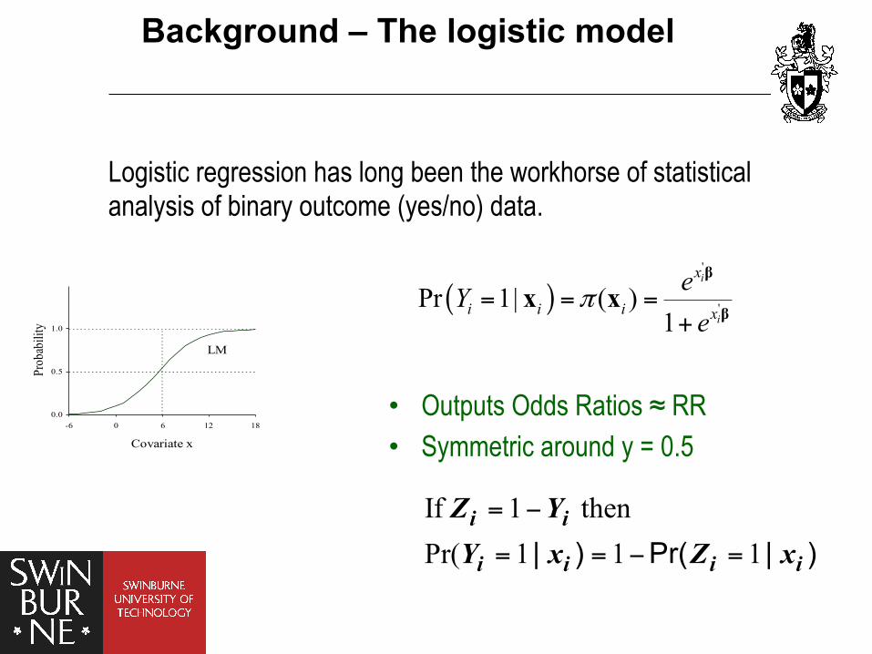
Logistic regression has long been the workhorse of statistical analysis of binary outcome (yes/no) data.

0.0

0.5

1.0

-6 0 6 12 18

Covariate x

Prob

abili

ty

LM

•  Outputs Odds Ratios ≈ RR •  Symmetric around y = 0.5

If 1 thenPr( 1 1 1| ) Pr( | )

i i

i i i i

Z YY x Z x= −

= = − =

( )'

'Pr 1| ( )1

i

i

x

i i i x

eYe

π= = =+

β

βx x

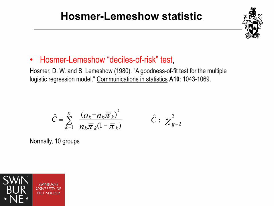
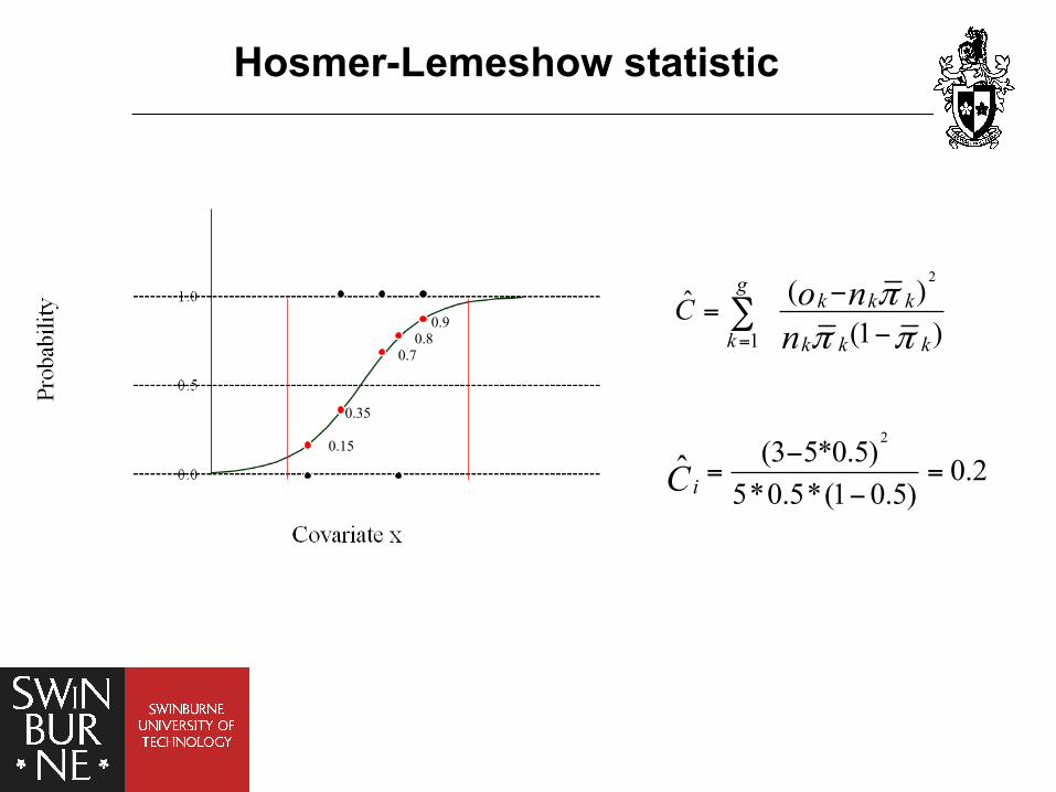
•  Hosmer-Lemeshow “deciles-of-risk” test, Hosmer, D. W. and S. Lemeshow (1980). "A goodness-of-fit test for the multiple logistic regression model." Communications in statistics A10: 1043-1069. Normally, 10 groups

2

1

( )ˆ(1 )

gk k k

k k k kC o n

nπ

π π=

−=

−∑ 2

2ˆ

gC χ −:

Hosmer-Lemeshow statistic

Menzies Research Institute

0.80.9

0.7

0.15

0.35

2(3 5*0.5) 0.25*0.5*(1 0.5)

ˆ iC−

= =−

2

1

( )ˆ(1 )

gk k k

k k k kC o n

nπ

π π=

−=

−∑

Hosmer-Lemeshow statistic

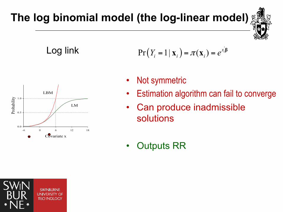
The log binomial model (the log-linear model)

•  Not symmetric •  Estimation algorithm can fail to converge •  Can produce inadmissible

solutions •  Outputs RR

0.0

0.5

1.0

-6 0 6 12 18

Covariate x

Prob

abili

ty

LBM

LM

Log link ( )'

Pr 1| ( )π= = = βx x ixi i iY e

Hjort-Hosmer statistic Hosmer DW, Hjort NL, (2002). “Goodness-of-fit processes for logistic regression: simulation results.” Statistics in medicine. 21(18), 2723-2738. Quinn SJ, Hosmer DW, Blizzard L, Goodness-of-fit statistics for log-link regression models. J Stat Comp Sim. 85(12) (2014), 2533-2545

Hjort–Hosmer recommended GOF statistic to assess log binomial regression

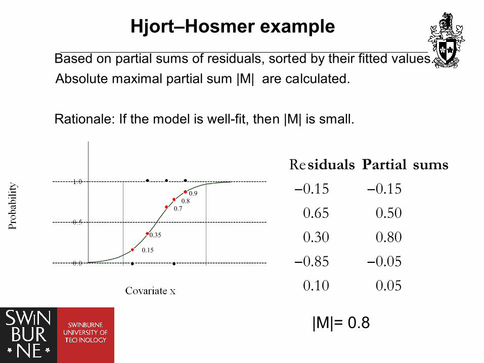
Hjort–Hosmer example

0.80.9

0.7

0.15

0.35

Re

0.15 0.15

0.65 0.50

0.30 0.80

0.85 0.05

0.10 0.05

siduals Partial sums

− −

− −

|M|= 0.8

Based on partial sums of residuals, sorted by their fitted values.Absolute maximal partial sum |M| are calculated.

Rationale: If the model is well-fit, then |M| is small.

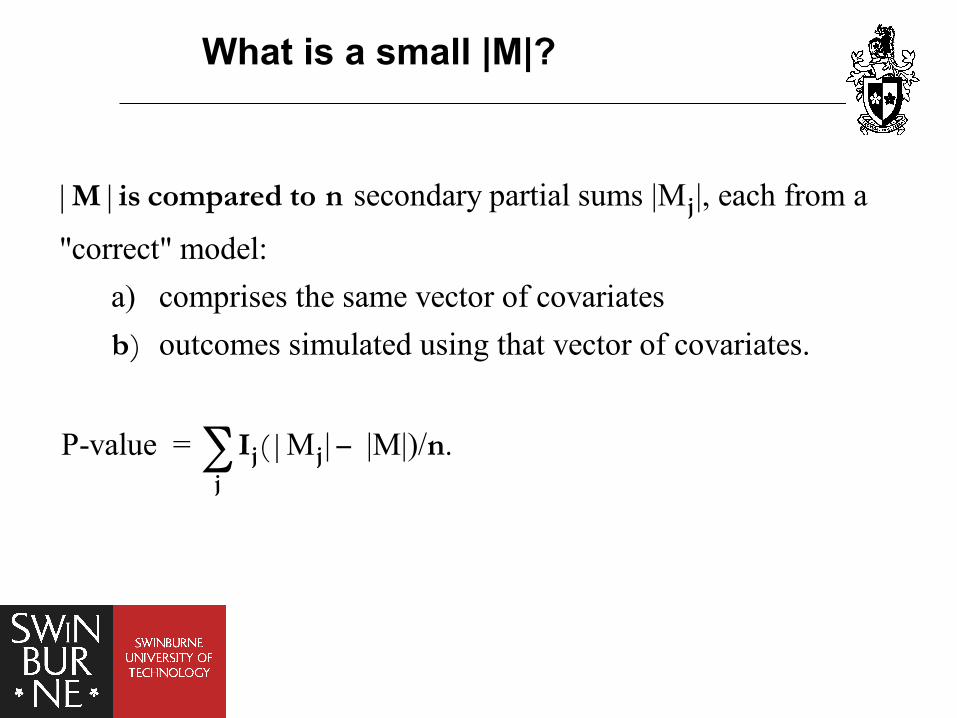
secondary partial sums |M |, each from a

"correct" model: a) comprises the same vector of covariates

outcomes simulated using that vector of covariates.

P-value = M | |M|)/

| |

)

(| .

j

j jj

M is compared to n

b

I n−∑

What is a small |M|?

Menzies Research Institute

Performance of HH vs. HL

•  The correct model

•  rejection rates of both HH and HL ≈ 5%

•  An incorrectly specified model

•  HH > HL by ≈ 10%

•  rejection rates of both HH and HL ≈ 5%

•  SUGM 2015

•  An ado file - hh.ado

Probit Complementary log-log (CLL) Log-log Arc-sin A corresponding study to that published in 2014 has been carried out for CLL •  Not symmetric •  Still used today

What about other forms of binary regression?

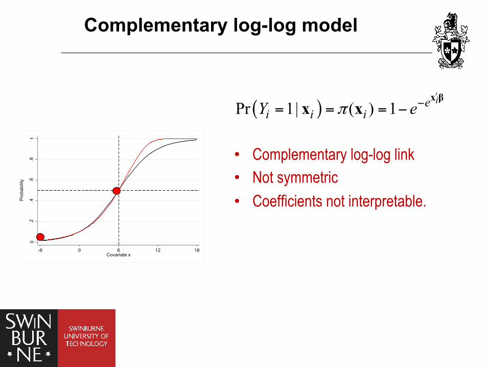
Complementary log-log model 0

.2.4

.6.8

1

Prob

abili

ty

-6 0 6 12 18Covariate x

•  Complementary log-log link •  Not symmetric •  Coefficients not interpretable.

( )Pr 1| ( ) 1πʹ−= = = −x β

x x iei i iY e

Why bother?

•  It has been used to calculate prevalence ratios (vs. prevalence odds ratios)

Bhattacharya R, Shen C, Sambamoorthi U, Excess risk of chronic physical conditions associated with depression and anxiety. BMC psychiatry. 14(2014), pp. 10.

•  It has been used based on a biological expectation of an asymmetrical relationship between the systematic and random components

Gyimah SO, Adjei JK, Takyi BK, Religion, contraception, and method choice of married women in Ghana. Journal of religion and health. 51(4) (2012), pp. 1359-1374.

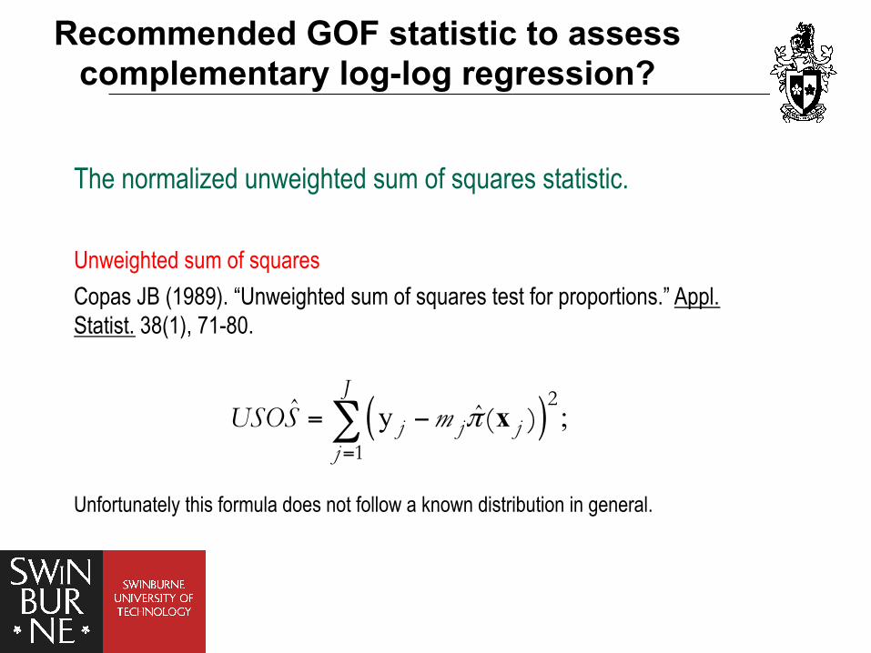
The normalized unweighted sum of squares statistic. Unweighted sum of squares Copas JB (1989). “Unweighted sum of squares test for proportions.” Appl. Statist. 38(1), 71-80.

Unfortunately this formula does not follow a known distribution in general.

Recommended GOF statistic to assess complementary log-log regression?

( )y ;=

= −∑ x2

1

ˆ ˆ( )J

j j jj

USOS m π

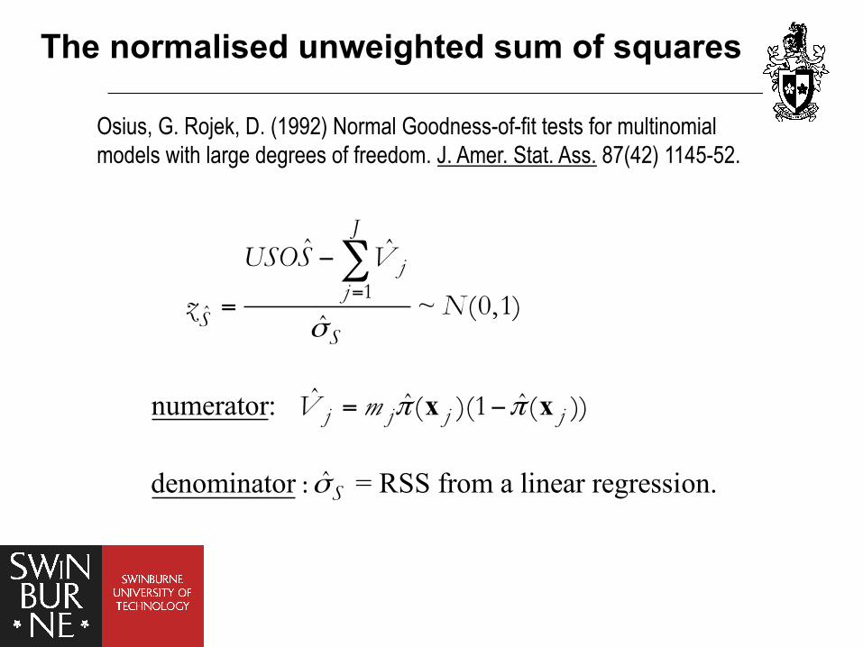
Osius, G. Rojek, D. (1992) Normal Goodness-of-fit tests for multinomial models with large degrees of freedom. J. Amer. Stat. Ass. 87(42) 1145-52.

The normalised unweighted sum of squares

numerator:

denominator = RSS from a linear regression.

=

−

=

= −

∑

x x

1ˆ

ˆ ˆ

~ (0,1)ˆ

ˆ ˆ ˆ( )(1 ( ))

ˆ:

J

jj

SS

j j j j

S

USOS V

z N

V m

σ

π π

σ

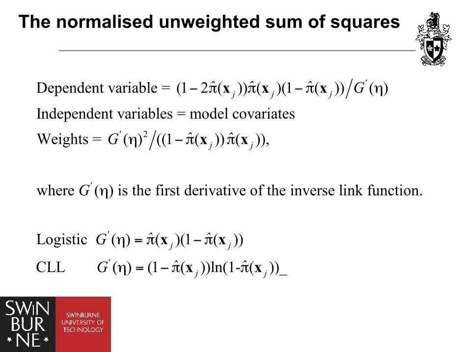
The normalised unweighted sum of squares

2

Dependent variable = (1 2 ( )) ( )(1 ( )) ( )

Independent variables = model covariatesWeights = ( ) ((1 ( )) ( )),

where ( ) is the first derivative of the inverse link function.

Logisti

'j j j

'j j

'

ˆ ˆ ˆ G

ˆ ˆG

G

− π π − π η

η − π π

η

x x x

x x

c ( ) ( )(1 ( ))

CLL ( ) (1 ( ))ln(1- ( ))_

'j j

'j j

ˆ ˆG

ˆ ˆG

η = π − π

η = − π π

x x

x x

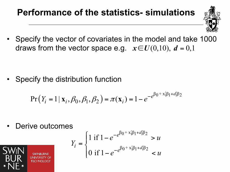
Performance of the statistics- simulations

•  Specify the vector of covariates in the model and take 1000 draws from the vector space e.g.

•  Specify the distribution function

•  Derive outcomes

( )β + x β β0 i 1 2

0 1 2Pr 1| , , , ( ) 1β β β πʹ ʹ+−= = = −

diei i iY ex x

β + x β β0 i 1 2

β + x β β0 i 1 2

1 if 1

0 if 1

di

di

e

ie

e uY

e u

ʹ ʹ+

ʹ ʹ+

−

−

⎧ − >⎪= ⎨⎪ − <⎩

(0,10), 0,1∈ =x U d

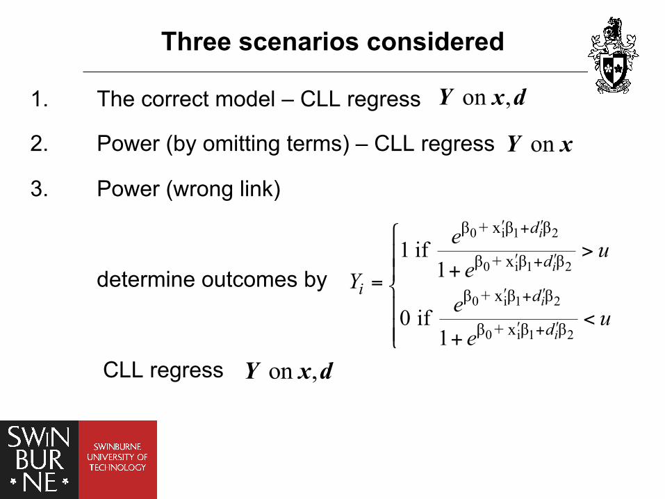
Three scenarios considered 1. The correct model – CLL regress

2. Power (by omitting terms) – CLL regress

3. Power (wrong link)

determine outcomes by

CLL regress

0 i 1 2

0 i 1 2

0 i 1 2

0 i 1 2

β + x β β

β + x β β

β + x β β

β + x β β

1 if 1

0 if 1

ʹ ʹ+

ʹ ʹ+

ʹ ʹ+

ʹ ʹ+

⎧>⎪

⎪ += ⎨⎪ <⎪⎩ +

i

i

i

i

d

d

i d

d

e ueYe ue

on ,Y x d

on Y x

on ,Y x d

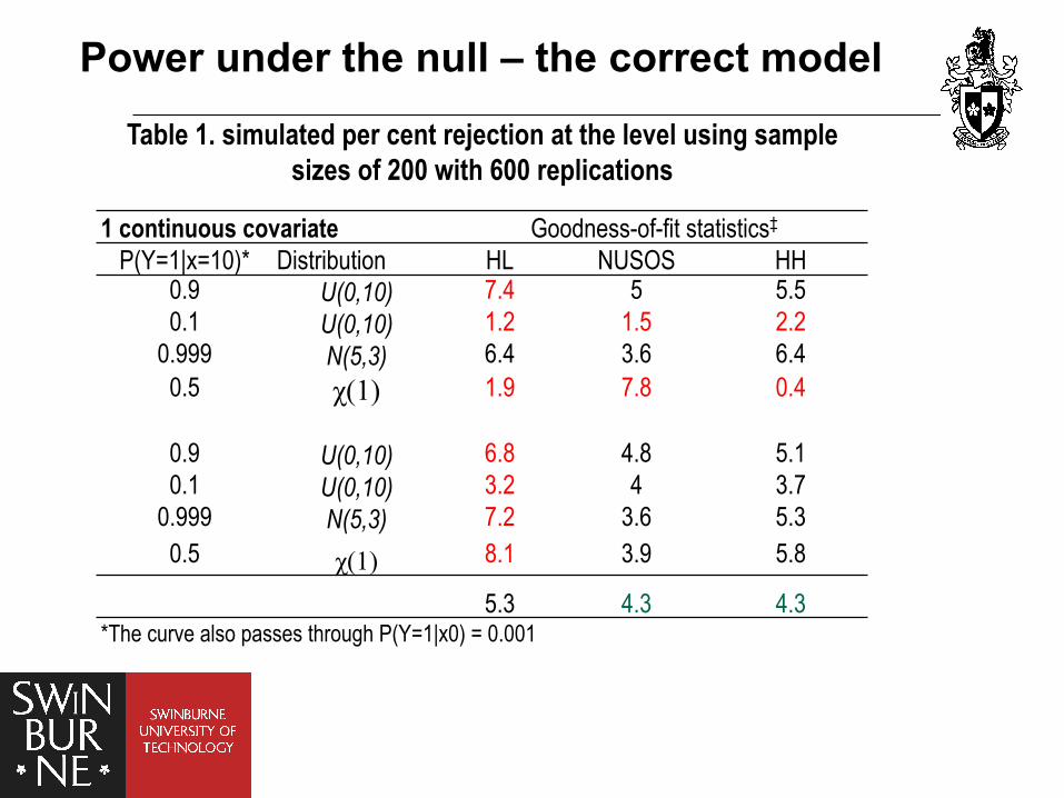
Power under the null – the correct model

Table 1. simulated per cent rejection at the level using sample sizes of 200 with 600 replications

1 continuous covariate Goodness-of-fit statistics‡

P(Y=1|x=10)* Distribution HL NUSOS HH 0.9 U(0,10) 7.4 5 5.5 0.1 U(0,10) 1.2 1.5 2.2

0.999 N(5,3) 6.4 3.6 6.4 0.5 χ(1) 1.9 7.8 0.4

0.9 U(0,10) 6.8 4.8 5.1 0.1 U(0,10) 3.2 4 3.7

0.999 N(5,3) 7.2 3.6 5.3 0.5 χ(1) 8.1 3.9 5.8

5.3 4.3 4.3 *The curve also passes through P(Y=1|x0) = 0.001

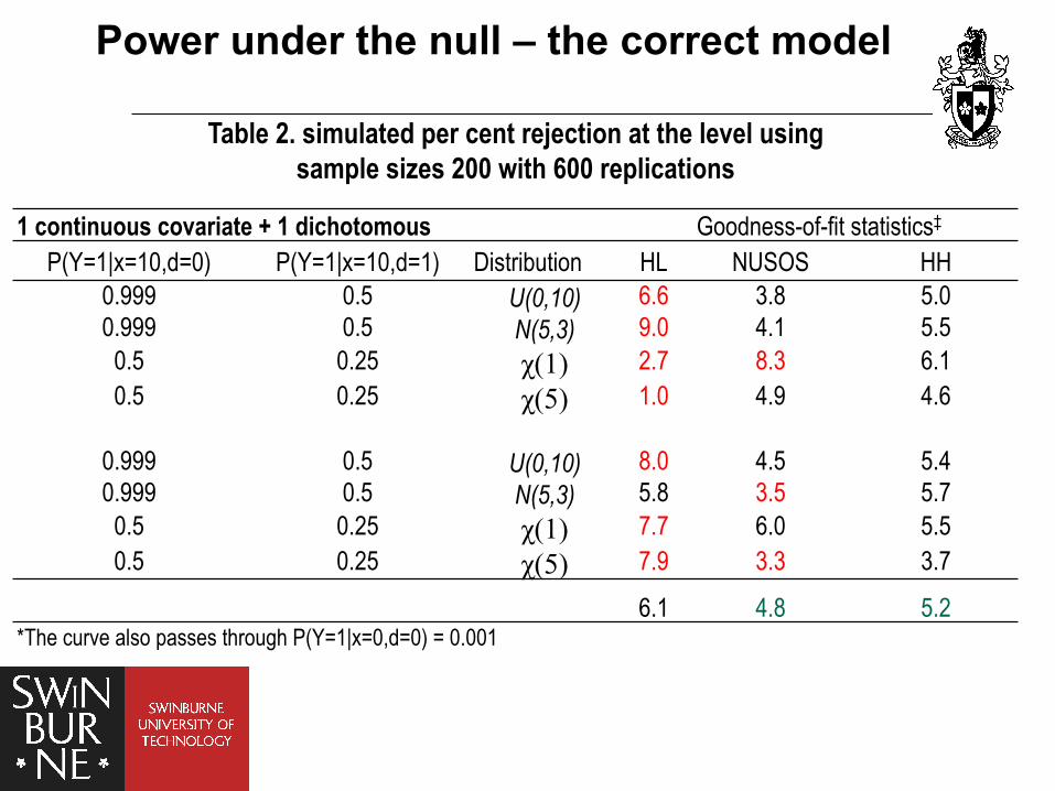
Table 2. simulated per cent rejection at the level using sample sizes 200 with 600 replications

1 continuous covariate + 1 dichotomous Goodness-of-fit statistics‡

P(Y=1|x=10,d=0) P(Y=1|x=10,d=1) Distribution HL NUSOS HH 0.999 0.5 U(0,10) 6.6 3.8 5.0 0.999 0.5 N(5,3) 9.0 4.1 5.5

0.5 0.25 χ(1) 2.7 8.3 6.1 0.5 0.25 χ(5) 1.0 4.9 4.6

0.999 0.5 U(0,10) 8.0 4.5 5.4 0.999 0.5 N(5,3) 5.8 3.5 5.7

0.5 0.25 χ(1) 7.7 6.0 5.5 0.5 0.25 χ(5) 7.9 3.3 3.7

6.1 4.8 5.2 *The curve also passes through P(Y=1|x=0,d=0) = 0.001

Power under the null – the correct model

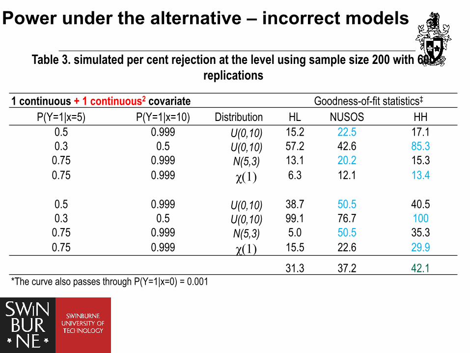
Table 3. simulated per cent rejection at the level using sample size 200 with 600 replications

1 continuous + 1 continuous2 covariate Goodness-of-fit statistics‡

P(Y=1|x=5) P(Y=1|x=10) Distribution HL NUSOS HH 0.5 0.999 U(0,10) 15.2 22.5 17.1 0.3 0.5 U(0,10) 57.2 42.6 85.3

0.75 0.999 N(5,3) 13.1 20.2 15.3 0.75 0.999 χ(1) 6.3 12.1 13.4

0.5 0.999 U(0,10) 38.7 50.5 40.5 0.3 0.5 U(0,10) 99.1 76.7 100

0.75 0.999 N(5,3) 5.0 50.5 35.3 0.75 0.999 χ(1) 15.5 22.6 29.9

31.3 37.2 42.1 *The curve also passes through P(Y=1|x=0) = 0.001

Power under the alternative – incorrect models

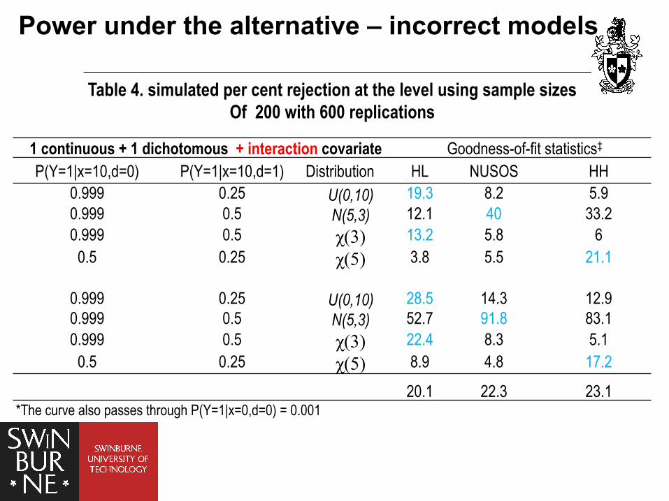
Table 4. simulated per cent rejection at the level using sample sizes Of 200 with 600 replications

1 continuous + 1 dichotomous + interaction covariate Goodness-of-fit statistics‡ P(Y=1|x=10,d=0) P(Y=1|x=10,d=1) Distribution HL NUSOS HH

0.999 0.25 U(0,10) 19.3 8.2 5.9 0.999 0.5 N(5,3) 12.1 40 33.2 0.999 0.5 χ(3) 13.2 5.8 6

0.5 0.25 χ(5) 3.8 5.5 21.1

0.999 0.25 U(0,10) 28.5 14.3 12.9 0.999 0.5 N(5,3) 52.7 91.8 83.1 0.999 0.5 χ(3) 22.4 8.3 5.1

0.5 0.25 χ(5) 8.9 4.8 17.2

20.1 22.3 23.1 *The curve also passes through P(Y=1|x=0,d=0) = 0.001

Power under the alternative – incorrect models

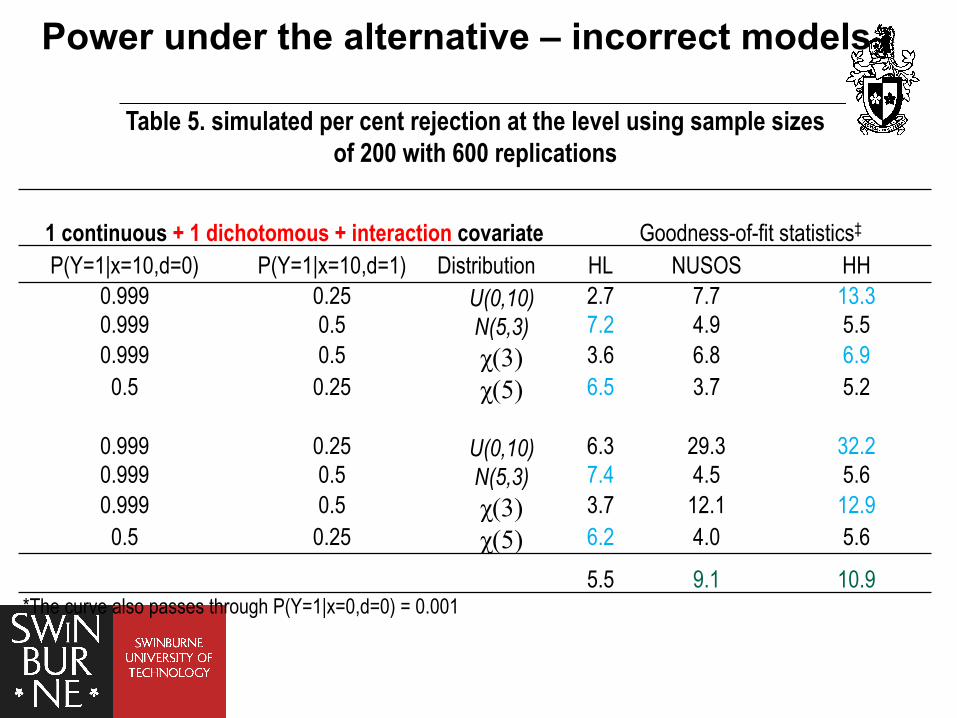
Table 5. simulated per cent rejection at the level using sample sizes of 200 with 600 replications

1 continuous + 1 dichotomous + interaction covariate Goodness-of-fit statistics‡ P(Y=1|x=10,d=0) P(Y=1|x=10,d=1) Distribution HL NUSOS HH

0.999 0.25 U(0,10) 2.7 7.7 13.3 0.999 0.5 N(5,3) 7.2 4.9 5.5 0.999 0.5 χ(3) 3.6 6.8 6.9

0.5 0.25 χ(5) 6.5 3.7 5.2

0.999 0.25 U(0,10) 6.3 29.3 32.2 0.999 0.5 N(5,3) 7.4 4.5 5.6 0.999 0.5 χ(3) 3.7 12.1 12.9

0.5 0.25 χ(5) 6.2 4.0 5.6

5.5 9.1 10.9 *The curve also passes through P(Y=1|x=0,d=0) = 0.001

Power under the alternative – incorrect models

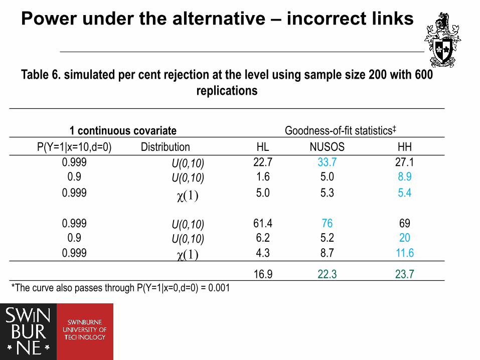
Table 6. simulated per cent rejection at the level using sample size 200 with 600 replications

1 continuous covariate Goodness-of-fit statistics‡ P(Y=1|x=10,d=0) Distribution HL NUSOS HH

0.999 U(0,10) 22.7 33.7 27.1 0.9 U(0,10) 1.6 5.0 8.9

0.999 χ(1) 5.0 5.3 5.4

0.999 U(0,10) 61.4 76 69 0.9 U(0,10) 6.2 5.2 20

0.999 χ(1) 4.3 8.7 11.6

16.9 22.3 23.7 *The curve also passes through P(Y=1|x=0,d=0) = 0.001

Power under the alternative – incorrect links

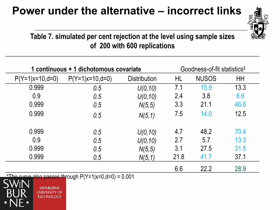
Table 7. simulated per cent rejection at the level using sample sizes of 200 with 600 replications

1 continuous + 1 dichotomous covariate Goodness-of-fit statistics‡ P(Y=1|x=10,d=0) P(Y=1|x=10,d=0) Distribution HL NUSOS HH

0.999 0.5 U(0,10) 7.1 15.9 13.3 0.9 0.5 U(0,10) 2.4 3.8 6.6

0.999 0.5 N(5,5) 3.3 21.1 46.6 0.999 0.5 N(5,1) 7.5 14.0 12.5

0.999 0.5 U(0,10) 4.7 48.2 70.4

0.9 0.5 U(0,10) 2.7 5.7 13.3 0.999 0.5 N(5,5) 3.1 27.5 31.5 0.999 0.5 N(5,1) 21.8 41.7 37.1

6.6 22.2 28.9 *The curve also passes through P(Y=1|x=0,d=0) = 0.001

Power under the alternative – incorrect links

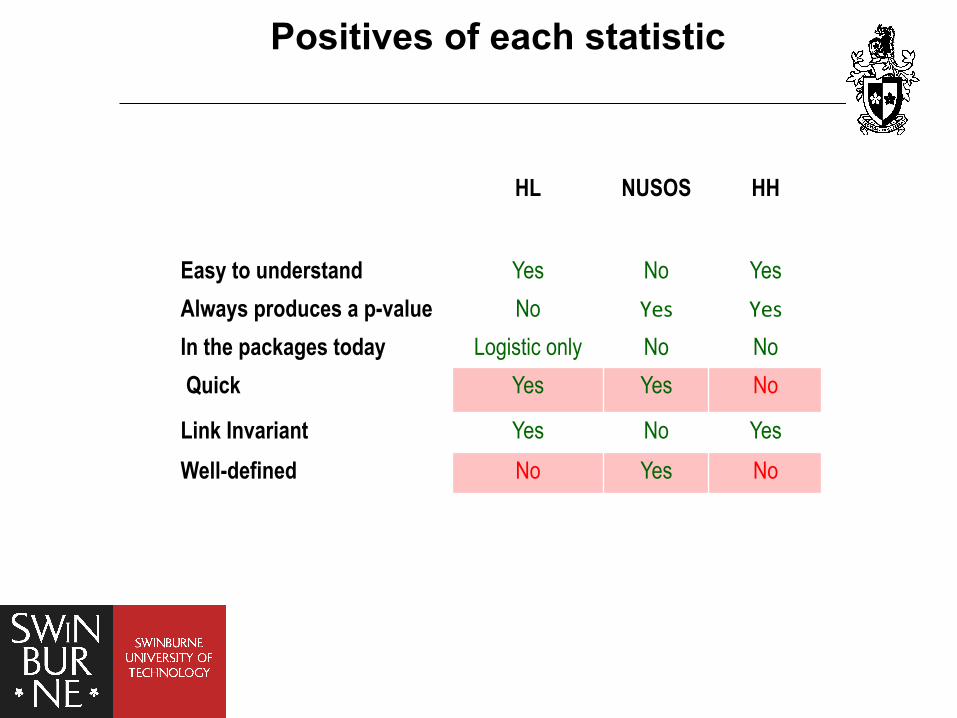
Positives of each statistic

  HL NUSOS HH

Easy to understand Yes No Yes Always produces a p-value No Yes Yes

In the packages today Logistic only No No Quick Yes Yes No

Link Invariant Yes No Yes Well-defined No Yes No

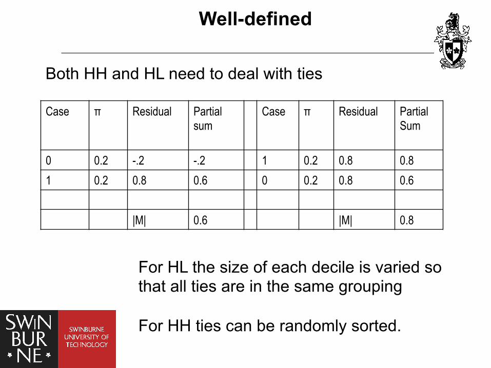
Well-defined

Both HH and HL need to deal with ties

Case π Residual Partial sum

Case π Residual Partial Sum

0 0.2 -.2 -.2 1 0.2 0.8 0.8 1 0.2 0.8 0.6 0 0.2 0.8 0.6

|M| 0.6 |M| 0.8

For HL the size of each decile is varied so that all ties are in the same grouping For HH ties can be randomly sorted.

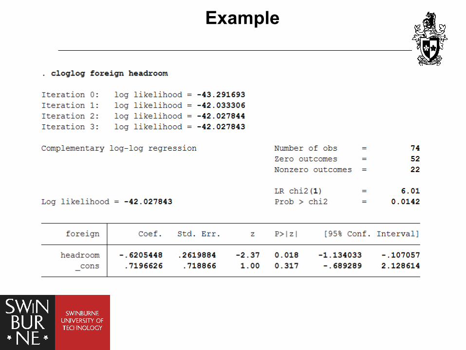
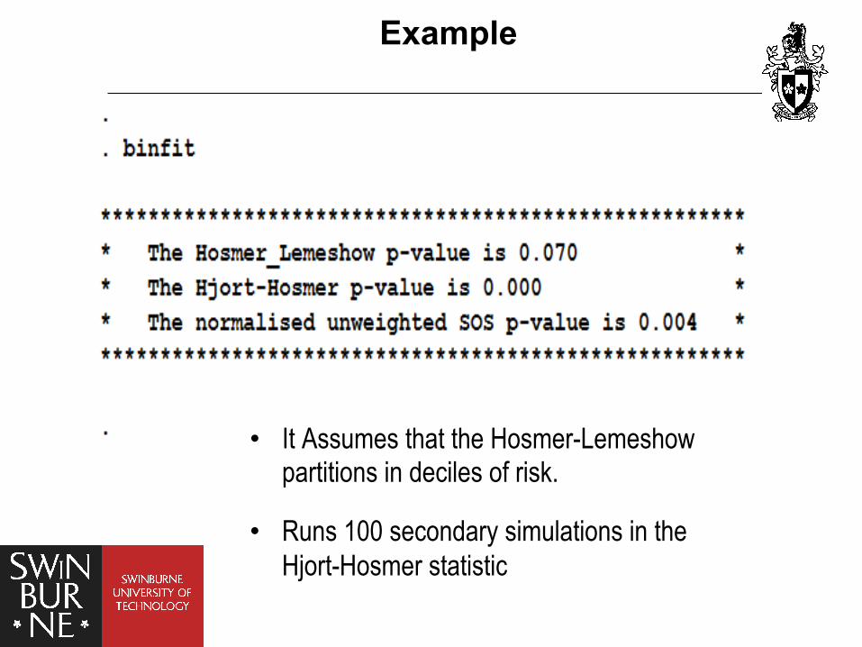
Example

Example

•  It Assumes that the Hosmer-Lemeshow partitions in deciles of risk.

•  Runs 100 secondary simulations in the Hjort-Hosmer statistic

Questions or comments ?