Newcastle University ePrints - eprint.ncl.ac.uk

Goodarzi M, Rouainia M, Aplin AC, Cubillas P, de Block M.

Predicting the elastic response of organic-rich shale using nanoscale

measurements and homogenisation methods.

Geophysical Prospecting (2017)

DOI: https://doi.org/10.1111/1365-2478.12475

Copyright:

This is the peer reviewed version of the following article, which has been published in final form at

https://doi.org/10.1111/1365-2478.12475. This article may be used for non-commercial purposes in

accordance with Wiley Terms and Conditions for Self-Archiving.

Date deposited:

23/10/2016

Embargo release date:

24 January 2018

Predicting the elastic response of organic-rich shaleusing nanoscale measurements and homogenisation

methods

M. Goodarzi1, M. Rouainia1, A.C. Aplin2, P. Cubillas2 and M. de Block31School of Civil Engineering and Geosciences, Newcastle University, Newcastle NE1 7RU, UK

2Department of Earth Sciences, Durham University, DH1 3LE, UK3SGS Horizon B.V., Stationsplein 6, Voorburg, 2275 AZ, Netherlands

Abstract

Determination of the mechanical response of shales throughexperimental proceduresis a practical challenge due to their heterogeneity and the practical difficulties of retrievinggood quality core samples. Here, we investigate the possibility of using multi-scale ho-mogenisation techniques to predict the macroscopic mechanical response of shales, basedon quantitative mineralogical descriptions. We use the novel PeakForce Quantitative Nanome-chanical Mapping (QNMr) technique to generate high resolution mechanical images ofshales, allowing the response of porous clay, organic matter and mineral inclusions to bemeasured at the nanoscale. These observations support someof the assumptions previouslymade in the use of homogenisation methods to estimate the elastic properties of shale,and also earlier estimates of the mechanical properties of organic matter. We evaluate theapplicability of homogenisation techniques against measured elastic responses of organic-rich shales, partly from published data and also from new indentation tests carried out inthis work. Comparison of experimental values of the elasticconstants of shale sampleswith those predicted by homogenisation methods showed thatalmost all predictions werewithin the standard deviation of experimental data. This suggests that the homogenisationapproach is a useful way of estimating the elastic and mechanical properties of shales, insituations where conventional rock mechanics test data cannot be measured.Key words: Anisotropy, Elastics, Imaging, Modelling, Rock physics.

1

1 Introduction1

Shale, or mudstone, is the most common sedimentary rock: a heterogeneous, multi-mineralic2

natural composite consisting of clay mineral aggregates, organic matter and variable quantities3

of minerals such as quartz, calcite and feldspar. Shale plays a key role as a top seal to many4

petroleum reservoirs and CO2 storage sites, as a low permeability barrier for nuclear waste and5

as an unconventional petroleum reservoir. In all these contexts, and as a material which needs to6

be effectively drilled when exploring for petroleum, the mechanical properties of shale are crit-7

ical but quite poorly constrained. For example, there are relatively few laboratory-based studies8

where mechanical data have been measured on shales which have been well-characterised in9

terms of mineralogy and microstructure. In part, this is dueto the chemical and mechanical10

instability of shales, which means that it is challenging and expensive to retrieve good quality11

core samples for undertaking conventional rock mechanics experiments (Kumar, Sondergeld12

and Rai 2012). Furthermore, because shales are heterogeneous on many scales (e.g. Aplin and13

Macquaker 2011), it is not straightforward to relate macroscopic experimental measurements to14

microscopic structural data.15

Recently, micromechanical indentation tests have been performed on shales (Zeszotarski et16

al. 2004; Ulm and Abousleiman 2006). Although this technique is fast and can be performed on17

commonly available drill cuttings, the data have limited scope as they cannot fully characterize18

the mechanical response of the material. However, indentation is useful for comparing the19

mechanical response of different materials. Another approach is to adopt micro-mechanical20

models that have been widely used in the field of composite engineering (Klusemann, Bohm21

and Svendsen 2012; Mortazavi et al. 2013). In these methods,the macroscale mechanical22

behaviour of a composite is determined from the mechanical response of each constituent along23

with their interaction with each other. This modelling approach is in principle well suited to24

shale, the mechanical properties of which are likely to depend on the porosity, the volume25

fraction of solid mineral inclusions and the amount of organic matter (Sayers 2013a).26

In their pioneering work on the micro-mechanical modellingof the anisotropic elastic re-27

sponse of shales, Hornby, Schwartz and Hudson (1994) assumed an isotropic intrinsic response28

for the solid unit of clay into which macroscopic anisotropywas introduced through platelet-29

shaped clay particles, their orientation and interparticle nanopores. Silt inclusions were then30

added as spherical isolated grains. Subsequent work modified this approach to provide an im-31

proved description of the elastic response of shales, including the incorporation of organic mat-32

ter into the shale microstructure model (Sayers 1994; Jakobson, Hudson and Johansen 2003;33

Ortega, Ulm and Abousleiman 2007; Zhu et al. 2012; Vasin et al. 2013; Sayers 2013a; Qin,34

Han and Zhao 2014). The main difference between these studies relates to the homogenisation35

strategies used to upscale the shale matrix (containing solid clay, kerogen and fluid phases), as36

well as the properties of the solid clay and kerogen. For example, Zhu et al. (2012) and Qin et37

al. (2014) considered kerogen as elliptical inclusions embedded into the shale microstructure.38

Guo, Li and Liu (2014) followed the same approach as Hornby etal. (1994), combining clay39

particles with kerogen and adding pores as spherical, isolated inclusions. In contrast, Vernik40

and Landis (1996) considered kerogen as an isotropic background matrix for the shale, which41

causes a reduction of the elastic constants. However, Sayers (2013b) showed that a model in42

which the matrix is described as a transversely isotropic (TI) kerogen and the shale as inclusion43

provides a better prediction of the elastic stiffness.44

Clearly, several quite different modelling approaches have been proposed to explain exper-45

imental observations, further highlighting the complexity of shales. In some studies (e.g. Wu46

et al. 2012; Zu et al. 2013), multiple micro-structural features, such as the amount of pores47

and their aspect ratios in both clay and kerogen, kerogen particle aspect ratio, cracks, etc., were48

considered numerically. However, these features could notbe directly measured and need to49

be calibrated. Although it is computationally possible to add any level of detail to a model, it50

should be noted that different combinations of these micro-structural features can produce the51

same overall mechanical response. Consequently, it is still difficult to be sure of the micro-52

structural factors which contribute most to the overall anisotropic response of shales (Bayuk,53

Ammerman and Chesnokov 2008).54

Two key issues need to be resolved in order to successfully implement multi-scale modelling55

approaches. Firstly, the mechanical properties of the elementary building blocks of shales must56

be known. Whilst the mechanical properties of phases such ascalcite and quartz are reason-57

ably well constrained, those of the solid unit of the porous clay and of organic matter are less58

well known. The second issue is the selection of an appropriate homogenisation strategy with59

which to account for the shale micro-structure and capture its behaviour at a macroscopic scale.60

With these two issues in mind, the objective of the present study is to assess the capabilities of61

multi-scale homogenisation methods to predict the elasticmechanical response of organic-rich62

shales using experimental measurements from nano to macro scales. In the first section, the63

adopted homogenisation formulation is discussed, along with its capabilities and limitations.64

Having described the input data required for this approach,we then use the recently developed65

Atomic Force Microscopy (AFM) technique, PeakForce QNMr, to investigate the nanoscale66

mechanical response of the individual phases, since these are fundamental inputs to the ho-67

mogenisation schemes. Published mechanical measurementsusing Ultra-sonic Pulse Velocity68

(UPV) test on core samples are then used to evaluate the predictions of the homogenisation69

method. Finally, indentation moduli measured parallel andperpendicular to bedding in several70

characterised organic-rich shale samples are used to further test the multi-scale homogenisation71

formulation for predicting the shale elastic response.72

2 Multi-scale homogenisation formulation73

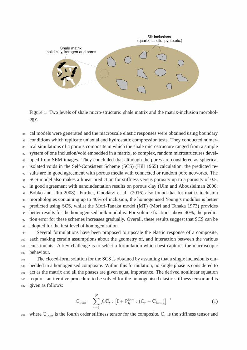
Here, shale is assumed to be a composite formed by a porous matrix in which solid mineral74

grains/inclusions are randomly distributed (Figure 1). Asa result, two levels of homogenisation75

need to be implemented for shales. At the first level, the properties of the shale matrix are76

upscaled using the porosity and properties of the solid unitof clay and organic matter. At the77

second level, the macroscale shale behaviour is obtained using the homogenised properties of78

the porous matrix from the previous level, plus the volume fractions and the properties of the79

different silt inclusions.80

Goodarzi, Rouainia and Aplin (2016) studied the performance and accuracy of various for-81

mulations using numerical analyses. Different microstructures for the porous clay and also82

the matrix-inclusion morphology were considered. Based onthese microstructures, numeri-83

Shale matrix

Silt Inclusions(quartz, calcite, pyrite,etc.)

solid clay, kerogen and pores

Figure 1: Two levels of shale micro-structure: shale matrixand the matrix-inclusion morphol-ogy.

cal models were generated and the macroscale elastic responses were obtained using boundary84

conditions which replicate uniaxial and hydrostatic compression tests. They conducted numer-85

ical simulations of a porous composite in which the shale microstructure ranged from a simple86

system of one inclusion/void embedded in a matrix, to complex, random microstructures devel-87

oped from SEM images. They concluded that although the poresare considered as spherical88

isolated voids in the Self-Consistent Scheme (SCS) (Hill 1965) calculation, the predicted re-89

sults are in good agreement with porous media with connectedor random pore networks. The90

SCS model also makes a linear prediction for stiffness versus porosity up to a porosity of 0.5,91

in good agreement with nanoindentation results on porous clay (Ulm and Abousleiman 2006;92

Bobko and Ulm 2008). Further, Goodarzi et al. (2016) also found that for matrix-inclusion93

morphologies containing up to 40% of inclusion, the homogenised Young’s modulus is better94

predicted using SCS, whilst the Mori-Tanaka model (MT) (Mori and Tanaka 1973) provides95

better results for the homogenised bulk modulus. For volumefractions above 40%, the predic-96

tion error for these schemes increases gradually. Overall,these results suggest that SCS can be97

adopted for the first level of homogenisation.98

Several formulations have been proposed to upscale the elastic response of a composite,99

each making certain assumptions about the geometry of, and interaction between the various100

constituents. A key challenge is to select a formulation which best captures the macroscopic101

behaviour.102

The closed-form solution for the SCS is obtained by assumingthat a single inclusion is em-103

bedded in a homogenised composite. Within this formulation, no single phase is considered to104

act as the matrix and all the phases are given equal importance. The derived nonlinear equation105

requires an iterative procedure to be solved for the homogenised elastic stiffness tensor and is106

given as follows:107

Chom =

N∑

r=1

frCr :[

I+ Phom

Ir: (Cr − Chom)

]

−1(1)

whereChom is the fourth order stiffness tensor for the composite,Cr is the stiffness tensor and108

fr is the volume fraction of the phaser, N is the total number of phases,I is the symmetric109

identity tensor, andPhom

Iris the Hill tensor which depends on the shape and the properties of110

the phase and the homogenised stiffness tensor of the composite. The stiffness tensor for a111

transversely isotropic material is described in terms of five independent components which can112

be written in the matrix notation as:113

C =

C11 C12 C13 0 0 0

C12 C11 C13 0 0 0

C13 C13 C33 0 0 0

0 0 0 2C44 0 0

0 0 0 0 2C44 0

0 0 0 0 0 2C66

with C66 =1

2

(

C11 − C12

)

(2)

The MT scheme, on the other hand, is based on the assumption that the inclusion is embed-114

ded in a layer of the matrix and an additional interaction term takes into account the effect of115

the adjacent inclusions. The final expression for MT scheme can be written as:116

Chom =N∑

r=1

frCr :[

I+ P0

Ir: (Cr − C0)

]

−1

[ N∑

s=0

fr[

I+ P0

Is: (Cs − C0)

]

−1

]

−1

(3)

whereC0 is the stiffness tensor for the matrix phase, andP0

Isis the Hill tensor which here it117

depends on the shape and the properties of the phaser and the homogenised stiffness tensor118

of the matrix. Obtaining the Hill’s tensor for the case of an anisotropic matrix is not trivial as119

it requires determination of Green’s function, which is extremely complicated for transversely120

isotropic materials (Laws 1977). Laws (1977) derived an integral expression for Hill’s tensor121

in this particular case which does not require knowledge of Green’s function. For explicit for-122

mulae of Hill’s tensor components for a spherical inclusionembedded in transversely isotropic123

matrices, readers are referred to Fritsch and Hellmich (2007). To the best of our knowledge,124

this is the only reference providing these expressions correctly.125

3 Material properties126

From equations (1) and (3), it can be seen that the volume fractions and the stiffness tensors of127

all constituents are required to allow the calculation of the homogenised elastic response of the128

composite. The volume fraction and mineralogy of clay and mineral inclusions can be estimated129

using X-ray diffraction, and the amount of organic matter measured by chemical analysis. A130

good estimation of the porosity, which can be measured in various ways, is also essential to the131

calculation of the clay matrix properties. The entire porosity of the sample is assumed to exist132

in the shale matrix, so that the porosity of the this matrix,φmatrix, which is used in the first level133

of homogenisation, is calculated as:134

φmatrix =φshale

1− finc(4)

whereφshale represents the shale porosity andfinc is the total volume of non-clay minerals.135

For dry conditions, porosity is taken to be a constituent with zero stiffness. However, in fully136

saturated shale, the stiffness properties of water within pores (i.e. bulk stiffnessK = 2.2 GPa137

and shear stiffnessG = 0 GPa) needs to be considered (Hornby et al. 1994; Vasin et al. 2013).138

Model implementation requires certain assumptions to be made about the properties of the139

different phases in shale. The shape and orientation of bothinclusions and pores are generally140

considered to be important sources of the macroscopic anisotropic response of shales (Vasin et141

al. 2013). Nanoscale indentation tests performed on several shale samples with a different level142

of porosity in their clay matrices revealed that the solid part of the porous clay exhibits a sig-143

nificant, intrinsic, anisotropic elastic response which gradually reduces with increasing porosity144

(Ulm and Abousleiman 2006; Bobko and Ulm 2008). Ortega, Ulm and Abousleiman (2010)145

used a micro-mechanical approach to study the simultaneouseffects of (a) anisotropy of the146

porous clay matrix, which was assumed to originate from solid clay particles, and (b) the shape147

and orientation of silt inclusions on the transversely isotropic elastic behaviour of bulk shale.148

They concluded that the possible contribution of the shape and orientation of silt inclusions on149

the macroscopic anisotropy of the shale is insignificant compared to the anisotropy of the clay150

matrix. This theoretical approach is also consistent with previous modelling and experimental151

studies in which an inverse correlation between silt inclusion content and anisotropy has been152

demonstrated (e.g. Bayuk et al. 2008; Guo et al. 2014).153

In addition, incorporating the effect of inclusion shape into multi-scale homogenisation re-154

quires additional experimental data which makes this approach inefficient from a practical point155

of view.156

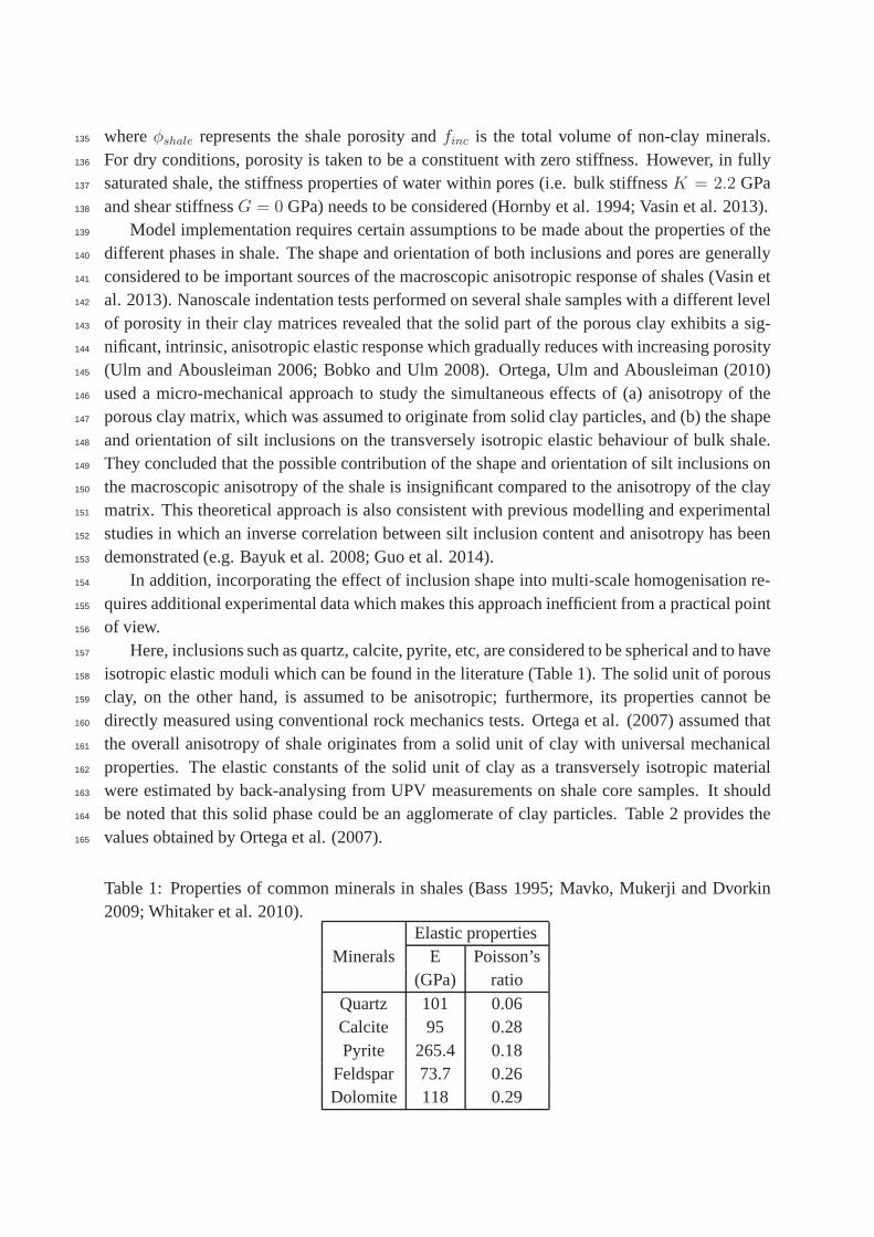
Here, inclusions such as quartz, calcite, pyrite, etc, are considered to be spherical and to have157

isotropic elastic moduli which can be found in the literature (Table 1). The solid unit of porous158

clay, on the other hand, is assumed to be anisotropic; furthermore, its properties cannot be159

directly measured using conventional rock mechanics tests. Ortega et al. (2007) assumed that160

the overall anisotropy of shale originates from a solid unitof clay with universal mechanical161

properties. The elastic constants of the solid unit of clay as a transversely isotropic material162

were estimated by back-analysing from UPV measurements on shale core samples. It should163

be noted that this solid phase could be an agglomerate of clayparticles. Table 2 provides the164

values obtained by Ortega et al. (2007).165

Table 1: Properties of common minerals in shales (Bass 1995;Mavko, Mukerji and Dvorkin2009; Whitaker et al. 2010).

Elastic propertiesMinerals E Poisson’s

(GPa) ratioQuartz 101 0.06Calcite 95 0.28Pyrite 265.4 0.18

Feldspar 73.7 0.26Dolomite 118 0.29

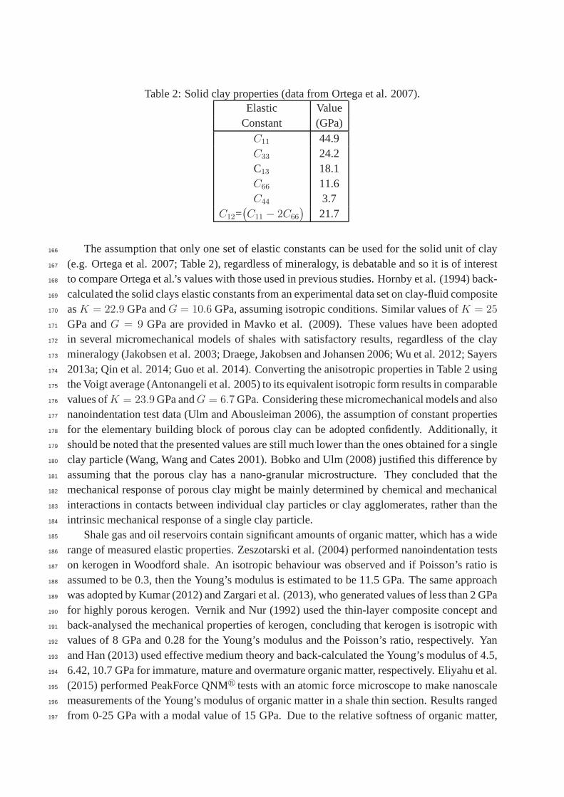
Table 2: Solid clay properties (data from Ortega et al. 2007).Elastic Value

Constant (GPa)C11 44.9C33 24.2C13 18.1C66 11.6C44 3.7

C12=(

C11 − 2C66

)

21.7

The assumption that only one set of elastic constants can be used for the solid unit of clay166

(e.g. Ortega et al. 2007; Table 2), regardless of mineralogy, is debatable and so it is of interest167

to compare Ortega et al.’s values with those used in previousstudies. Hornby et al. (1994) back-168

calculated the solid clays elastic constants from an experimental data set on clay-fluid composite169

asK = 22.9 GPa andG = 10.6 GPa, assuming isotropic conditions. Similar values ofK = 25170

GPa andG = 9 GPa are provided in Mavko et al. (2009). These values have been adopted171

in several micromechanical models of shales with satisfactory results, regardless of the clay172

mineralogy (Jakobsen et al. 2003; Draege, Jakobsen and Johansen 2006; Wu et al. 2012; Sayers173

2013a; Qin et al. 2014; Guo et al. 2014). Converting the anisotropic properties in Table 2 using174

the Voigt average (Antonangeli et al. 2005) to its equivalent isotropic form results in comparable175

values ofK = 23.9GPa andG = 6.7GPa. Considering these micromechanical models and also176

nanoindentation test data (Ulm and Abousleiman 2006), the assumption of constant properties177

for the elementary building block of porous clay can be adopted confidently. Additionally, it178

should be noted that the presented values are still much lower than the ones obtained for a single179

clay particle (Wang, Wang and Cates 2001). Bobko and Ulm (2008) justified this difference by180

assuming that the porous clay has a nano-granular microstructure. They concluded that the181

mechanical response of porous clay might be mainly determined by chemical and mechanical182

interactions in contacts between individual clay particles or clay agglomerates, rather than the183

intrinsic mechanical response of a single clay particle.184

Shale gas and oil reservoirs contain significant amounts of organic matter, which has a wide185

range of measured elastic properties. Zeszotarski et al. (2004) performed nanoindentation tests186

on kerogen in Woodford shale. An isotropic behaviour was observed and if Poisson’s ratio is187

assumed to be 0.3, then the Young’s modulus is estimated to be11.5 GPa. The same approach188

was adopted by Kumar (2012) and Zargari et al. (2013), who generated values of less than 2 GPa189

for highly porous kerogen. Vernik and Nur (1992) used the thin-layer composite concept and190

back-analysed the mechanical properties of kerogen, concluding that kerogen is isotropic with191

values of 8 GPa and 0.28 for the Young’s modulus and the Poisson’s ratio, respectively. Yan192

and Han (2013) used effective medium theory and back-calculated the Young’s modulus of 4.5,193

6.42, 10.7 GPa for immature, mature and overmature organic matter, respectively. Eliyahu et al.194

(2015) performed PeakForce QNMr tests with an atomic force microscope to make nanoscale195

measurements of the Young’s modulus of organic matter in a shale thin section. Results ranged196

from 0-25 GPa with a modal value of 15 GPa. Due to the relative softness of organic matter,197

the mechanical behaviour of shales may be significantly influenced by even small amounts198

of organic matter (Vernik and Milovac 2011; Sayers 2013b). This can lead to difficulties in199

implementing homogenisation techniques for these materials.200

4 Nanoscale mechanical mapping of shales201

Since shales are mainly formed of particles which range in size from smaller than 0.1 microns202

to 100 microns, it follows that a high resolution technique is required to measure the mechanical203

properties of individual particles or constituents in situ. Conventional small-scale mechanical204

testing methods such as indentation can extract discontinuous data, but only at a resolution of at205

least several microns. In contrast, the recently developedAFM technique known as PeakForce206

QNMr is a non-destructive method which measures the elastic response of a material surface207

with a resolution of a few nanometres. In this mode, an AFM probe is tapped over the surface208

(using a sinusoidal signal) and the peak force applied on thesurface is used as a feedback pa-209

rameter to track the scanned surface (i.e. the peak force is continuously monitored and kept210

constant during scanning). The mechanical response of the sample is extracted using the gen-211

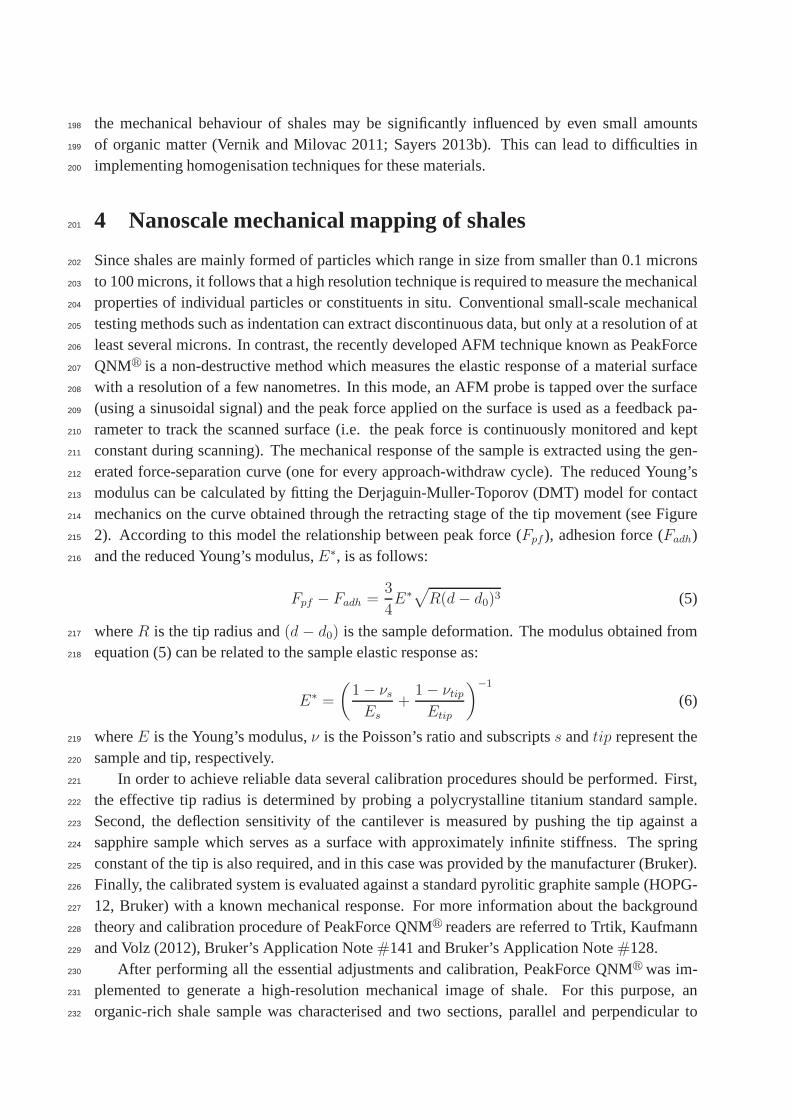
erated force-separation curve (one for every approach-withdraw cycle). The reduced Young’s212

modulus can be calculated by fitting the Derjaguin-Muller-Toporov (DMT) model for contact213

mechanics on the curve obtained through the retracting stage of the tip movement (see Figure214

2). According to this model the relationship between peak force (Fpf ), adhesion force (Fadh)215

and the reduced Young’s modulus,E∗, is as follows:216

Fpf − Fadh =3

4E∗

√

R(d− d0)3 (5)

whereR is the tip radius and(d − d0) is the sample deformation. The modulus obtained from217

equation (5) can be related to the sample elastic response as:218

E∗ =

(

1− νsEs

+1− νtipEtip

)

−1

(6)

whereE is the Young’s modulus,ν is the Poisson’s ratio and subscriptss andtip represent the219

sample and tip, respectively.220

In order to achieve reliable data several calibration procedures should be performed. First,221

the effective tip radius is determined by probing a polycrystalline titanium standard sample.222

Second, the deflection sensitivity of the cantilever is measured by pushing the tip against a223

sapphire sample which serves as a surface with approximately infinite stiffness. The spring224

constant of the tip is also required, and in this case was provided by the manufacturer (Bruker).225

Finally, the calibrated system is evaluated against a standard pyrolitic graphite sample (HOPG-226

12, Bruker) with a known mechanical response. For more information about the background227

theory and calibration procedure of PeakForce QNMr readers are referred to Trtik, Kaufmann228

and Volz (2012), Bruker’s Application Note#141 and Bruker’s Application Note#128.229

After performing all the essential adjustments and calibration, PeakForce QNMr was im-230

plemented to generate a high-resolution mechanical image of shale. For this purpose, an231

organic-rich shale sample was characterised and two sections, parallel and perpendicular to232

DTM fit formodulus

Approach

Withdraw

Tip position

Deformation

Adhesio

nP

eak

forc

e

Figure 2: Schematic diagram of a generated force-separation curve for a single tapping of thePeakForce QNMr (Modified from Bruker’s Application Note#128).

the bedding plane, were prepared (Table 3). Since a smooth surface is a key condition for233

good quality data in PeakForce QNMr and Indentation tests, the surfaces were hand polished234

and then polished using argon ion milling (Amirmajdi et al. 2009). Additionally, a suitable235

cantilever-tip assembly (with a relatively large stiffness> 200 Nm−1) is required to be able to236

measure the modulus on a shale, which contains stiff mineralgrains (E > 50 GPa) such as237

quartz. A diamond tip with a spring constant of 272 Nm−1 (DNISP; Bruker) was selected for238

this study. The tip was oscillated with 1 kHz frequency and the peak force was set to 50−239

150 nN, as this provided the best results during the tests performed on the HOPG-12 standard.240

These settings generated 1-2 nm indentation depths on the sample.241

Table 3: Characterisation of shale sample for the PeakForceQNMr test.Mineralogy Volume fraction

(%)Quartz 16.78Calcite 0.23Pyrite 2.91Feldspar 0.59Dolomite 0.00Clay 65.97Total organic Weightcarbon (TOC) (%)

5.83Porosity 9.45

4.1 Nano-mechanical image analysis242

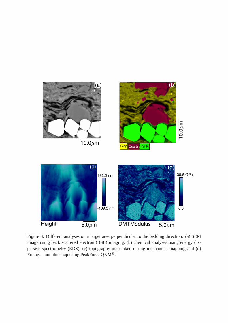
Figure 3 shows the elastic modulus map obtained on a 25×25 µm2 area on the shale sample243

perpendicular to the bedding direction (Figure 3d). Two types of grains with different, and244

relatively high stiffness (> 50 GPa); and also areas with very low stiffness (< 30 GPa) can245

be clearly recognised in this image. In order to better interpret the elastic modulus map, more246

analyses including back-scattered electron (BSE) SEM imaging, energy dispersive spectroscopy247

(EDS) chemical analysis and topographical data were also obtained from the same area (Figure248

3). As part of the data analysis, it was initially assumed that the stiffer grains represent pyrite249

(and were later identified as such from the EDS analysis (Figure 3b). An average value above250

100 GPa was measured on pyrite grains which is lower than the reported values of 265 GPa251

in the literature (see Table 1). The main reason for this deviation is that the reliable range of252

measurable elastic modulus for the diamond tip is less than 80 GPa (Bruker’s Application Note253

#128). The mean value of the measured Young’s modulus over thegrains corresponding to254

quartz in the EDS analysis (Figure 3b) is around 75 GPa, lowerthan the value reported in Table255

1 but between the values reported by Elihayu et al. (2015), 63± 8 GPa, and Mavko et al.256

(2009), 77− 95 GPa. Again, it is difficult to be certain of this result because of the reliable257

range of the tip.258

Due to the stiffness difference of shale constituents, it isnot possible to prepare a surface259

as smooth as single phase materials such as the pyrolitic graphite sample which is used for the260

calibration. Sample roughness may yield unreliable data. Comparing the topographical and the261

mechanical maps (Figures 3c and 3d), it can be concluded thatsome soft areas are correlated262

with abrupt deep areas on the sample. In fact, unlike the interpretation made by Eliyahu et al.263

(2015), not all the soft regions can be attributed to organicmatter and a careful comparison264

between both the mechanical and topographical images is required to locate real soft phases265

in the mechanical image. Such a comparison revealed the factthat the presence of the organic266

matter phase in the shale composite is not similar to other inclusions such as quartz and pyrite.267

This phase is intimately mixed within the porous clay ratherthan existing as isolated grains; this268

is important when accounting for organic matter in the homogenisation techniques. Assuming269

Poisson’s ratio is 0.3 for this phase, the measured Young’s moduli are less than 10 GPa with a270

mean value of 6 GPa. Considering that the maturity of this sample is at a vitrinite reflectance of271

0.5− 0.6% (Ro), this result is consistent with the values of 6− 9 GPa for immature kerogen272

obtained by Kumar (2012).273

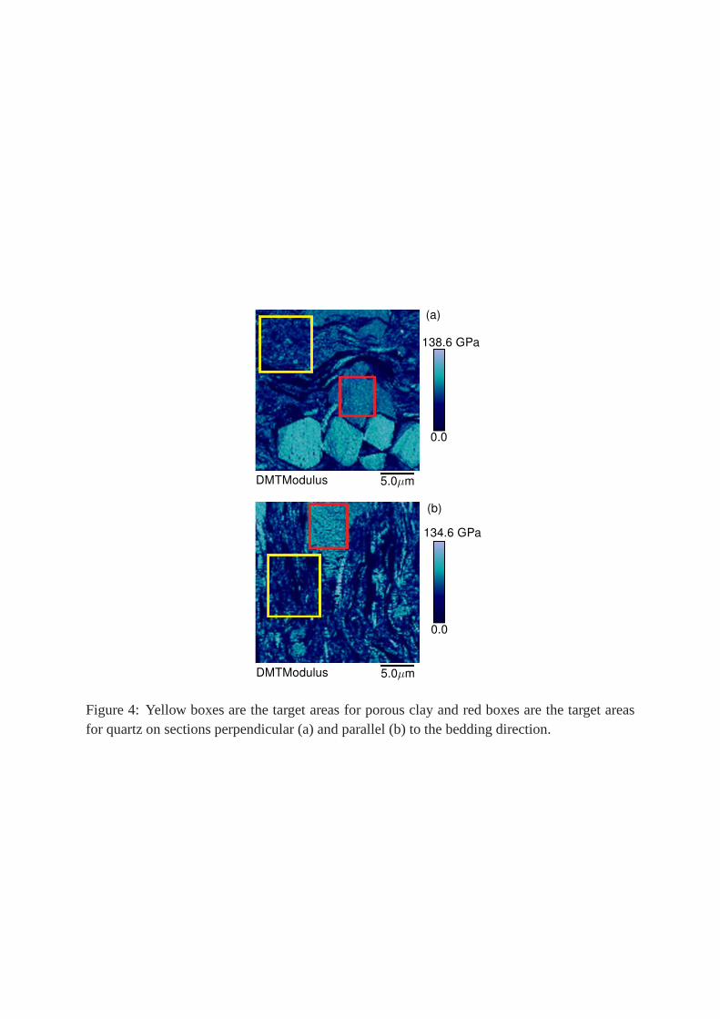
As the macroscopic response of shales is highly anisotropic, it is of interest to look at274

anisotropy at the nanoscale. Figure 4 shows the Young’s modulus map of sections both par-275

allel (E1) and perpendicular (E3) to the bedding direction. Two target areas were selected on276

both images that contained porous clay and quartz grains. The measured data in these areas277

were extracted and subjected to statistical analysis. Figure 5 illustrates the histogram and nor-278

mal curve on the data and the mean values and standard deviations (SD) are provided in Table279

4.280

The mean values obtained on quartz grains are almost identical, producing an anisotropy281

ratio (E1/E3) around 0.95. Although the measurements were taken from twodifferent grains282

with unknown orientations, this can be interpreted as an isotropic response for this phase. The283

DMTModulus 5.0µm

10.0µm

10.0µ

m

Clay PyriteQuartz

5.0µm

(a)

(c) (d)

(b)

Height

0.0

192.0 nm 138.6 GPa

-169.3 nm

Figure 3: Different analyses on a target area perpendicularto the bedding direction. (a) SEMimage using back scattered electron (BSE) imaging, (b) chemical analyses using energy dis-persive spectrometry (EDS), (c) topography map taken during mechanical mapping and (d)Young’s modulus map using PeakForce QNMr.

(a)

(b)

DMTModulus

DMTModulus 5.0µm

5.0µm

0.0

138.6 GPa

0.0

134.6 GPa

Figure 4: Yellow boxes are the target areas for porous clay and red boxes are the target areasfor quartz on sections perpendicular (a) and parallel (b) tothe bedding direction.

Figure 5: Histogram and normal curve of the measured Young’smoduli on (a) porous clay and(b) quartz grain in both sections parallel and perpendicular to bedding direction.

observed, in situ elastic response of quartz grains within shale microstructure is different to284

measurements on large quartz crystals, which show noticeable anisotropy (Heyliger, Ledbetter285

and Kim 2003). Vasin et al. (2013) considered the full anisotropic elastic response of silt286

inclusions with random orientations in modelling shale anisotropy. However, since quartz grains287

in shales are randomly orientated with respect to the crystal structure, our observation supports288

the simple assumption made in Hornby et al. (1994) that accounts for mineral inclusions as a289

spherical, elastically isotropic phase.290

The porous clay, on the other hand, shows significant anisotropy in these two sections with291

a ratio (E1/E3) around 1.45. An anisotropic ratio of 1.54 was obtained for ashale sample with292

almost the same porosity and inclusion volume fraction using UPV measurement on core sam-293

ples (Ulm and Abousleiman 2006). This comparison provides more support for the assumption,294

discussed in Section 3, about the origin of shale anisotropy. Additionally, the values obtained295

on the porous clay are higher than the properties assumed fora solid unit of porous clay here or296

the properties obtained by Hornby et al. (1994) (Table 2), but they are within the range of the297

properties reported for clay particles (Wang et al. 2001). Eliahayu et al. (2015) reported 29±298

1 GPa on the porous clay while they did not consider the direction of the section in their study.299

This value is very close to the measured data on the section perpendicular to bedding (see Table300

4). Further study is required to understand what type of micro-component of the porous clay301

was being touched by the tip.302

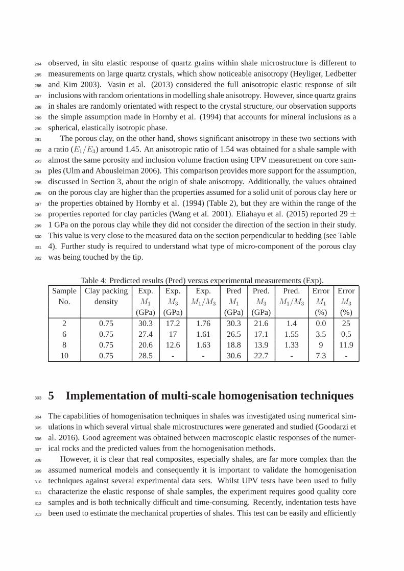
Table 4: Predicted results (Pred) versus experimental measurements (Exp).Sample Clay packing Exp. Exp. Exp. Pred Pred. Pred. Error Error

No. density M1 M3 M1/M3 M1 M3 M1/M3 M1 M3

(GPa) (GPa) (GPa) (GPa) (%) (%)2 0.75 30.3 17.2 1.76 30.3 21.6 1.4 0.0 256 0.75 27.4 17 1.61 26.5 17.1 1.55 3.5 0.58 0.75 20.6 12.6 1.63 18.8 13.9 1.33 9 11.910 0.75 28.5 - - 30.6 22.7 - 7.3 -

5 Implementation of multi-scale homogenisation techniques303

The capabilities of homogenisation techniques in shales was investigated using numerical sim-304

ulations in which several virtual shale microstructures were generated and studied (Goodarzi et305

al. 2016). Good agreement was obtained between macroscopicelastic responses of the numer-306

ical rocks and the predicted values from the homogenisationmethods.307

However, it is clear that real composites, especially shales, are far more complex than the308

assumed numerical models and consequently it is important to validate the homogenisation309

techniques against several experimental data sets. WhilstUPV tests have been used to fully310

characterize the elastic response of shale samples, the experiment requires good quality core311

samples and is both technically difficult and time-consuming. Recently, indentation tests have312

been used to estimate the mechanical properties of shales. This test can be easily and efficiently313

performed on shale cuttings and a good estimation on the anisotropic macroscopic elastic re-314

sponse of shale can be obtained (Kumar et al. 2012; Ulm and Abousleiman 2006). Here,315

published UPV results on well-characterised shales are used to evaluate the predictive capa-316

bility of the homogenisation techniques. In addition, several organic-rich shale samples were317

prepared, characterized and used to generate indentation data in order to extend the validation318

data sets.319

5.1 Elastic response of shales porous clay320

The mechanical response of silt-grade mineral inclusions in shales are well known and possible321

shape effects can be quantified using SEM or 3-D X-ray microtomographic imaging (Kanit-322

panyacharoen et al. 2011; Vasin et al. 2013; Peng et al. 2015). However, neither the exact323

microstructure of the porous clay, nor the properties of thesolid unit of this composite, have324

been fully evaluated. A complex network of pores including connected channels and isolated325

pores at different scales have been experimentally observed in porous clay (e.g. Chalmers,326

Bustin and Power 2012). Similarly, the organic matter occurs as a semi-continuous phase rather327

than as isolated inclusions in the porous clay (see Figure 3). Consequently, the main challenge328

in modelling the elastic behaviour of shales is the responseof the matrix.329

The main assumption in our approach is that the anisotropy originates from the solid clay,330

having a transversely elastic response. The Self-Consistent Scheme is used to combine, without331

any specific orientation distribution, the solid clay with the presence of pores and organic matter.332

Aligned, platy clay minerals are not considered explicitlyand the TI response compensates for333

this effect. On the other hand, Hornby et al. (1994) assumed an isotropic response for the solid334

clay and the anisotropy was subsequently generated by considering an oblate spheroid-shaped335

clay particles and nanopores. The SCS was combined with a differential effective medium336

model in order to satisfy the continuity of all the phases at any porosity level.337

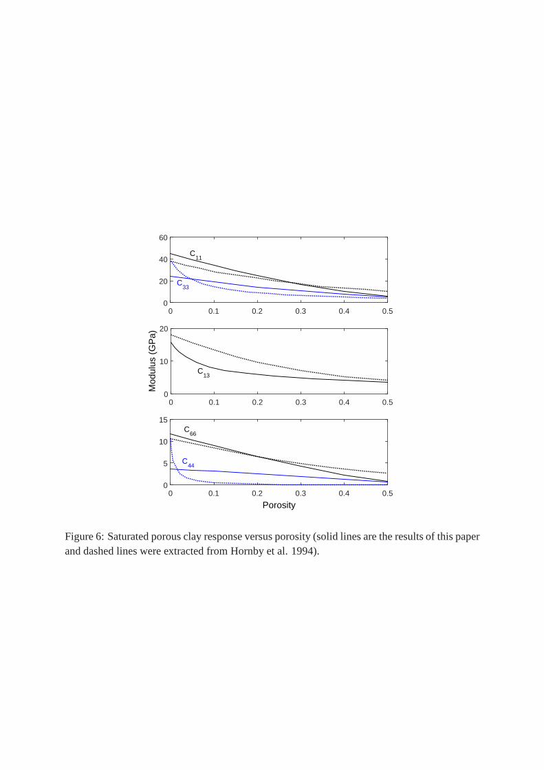
In order to clarify similarities and differences between the approach adopted in this paper338

and the pioneering work of Hornby et al. (1994), all five elastic constants of a fully-saturated339

porous clay are plotted as a function of porosity in Figure 6.Both approaches provide a similar340

trend for the elastic constants as functions of fluid-filled porosity except forC44, which shows341

a drastic decrease with a small increase in porosity in the Hornby et al. (1994) formulation.342

Additional differences can be partly attributed to the initial assumptions with regard to the343

isotropy and anisotropy of the elastic properties of the solid unit of clay. It should be noted344

that an increase or decrease in anisotropy can of course be introduced by considering elliptical345

shapes with specific orientations for pores or organic matter in the SCS formulation. These two346

modelling approaches give quite consistent results in reproducing the response of porous clay.347

5.2 UPV test data sets348

There are very few measurements of the mechanical behaviourof shales which are well char-349

acterised in terms of both mineralogy and microstrcture. Among these available data, those350

which were not used by Ortega et al. (2007) to back-calculatethe stiffness of the solid unit of351

porous clay, were chosen for this study. Table 5 provides themineralogical descriptions of these352

0 0.1 0.2 0.3 0.4 0.50

20

40

60

0 0.1 0.2 0.3 0.4 0.5

Mod

ulus

(G

Pa)

0

10

20

Porosity0 0.1 0.2 0.3 0.4 0.5

0

5

10

15

C11

C13

C66

C33

C44

Figure 6: Saturated porous clay response versus porosity (solid lines are the results of this paperand dashed lines were extracted from Hornby et al. 1994).

samples. For the first two data sets, Kimmeridge and Jurassicshales, the elastic constants were353

measured in saturated conditions under different confiningpressures. With increasing confining354

pressure, properties almost converged to constant values which we infer are due to the closure355

of microcracks. As cracks are not considered in our modelling, the values corresponding to356

the highest confining pressure, 80 MPa, were selected for comparison. For Woodford shales357

the natural water content of the samples was preserved but noinformation was provided on the358

confining pressure.359

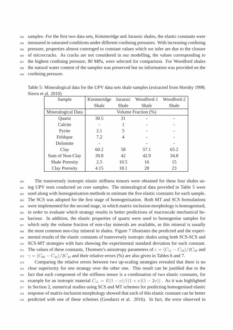
Table 5: Mineralogical data for the UPV data sets shale samples (extracted from Hornby 1998;Sierra et al. 2010)

Sample Kimmeridge Jurassic Woodford-1 Woodford-2Shale Shale Shale Shale

Mineralogical Data Volume Fraction (%)Quartz 30.5 31 - -Calcite - 1 - -Pyrite 2.1 5 - -

Feldspar 7.2 4 - -Dolomite - - -

Clay 60.2 58 57.1 65.2Sum of Non-Clay 39.8 42 42.9 34.8

Shale Porosity 2.5 10.5 16 15Clay Porosity 4.15 18.1 28 23

The transversely isotropic elastic stiffness tensors wereobtained for these four shales us-360

ing UPV tests conducted on core samples. The mineralogical data provided in Table 5 were361

used along with homogenisation methods to estimate the five elastic constants for each sample.362

The SCS was adopted for the first stage of homogenisation. Both MT and SCS formulations363

were implemented for the second stage, in which matrix-inclusion morphology is homogenised,364

in order to evaluate which strategy results in better predictions of macroscale mechanical be-365

haviour. In addition, the elastic properties of quartz wereused to homogenise samples for366

which only the volume fraction of non-clay minerals are available, as this mineral is usually367

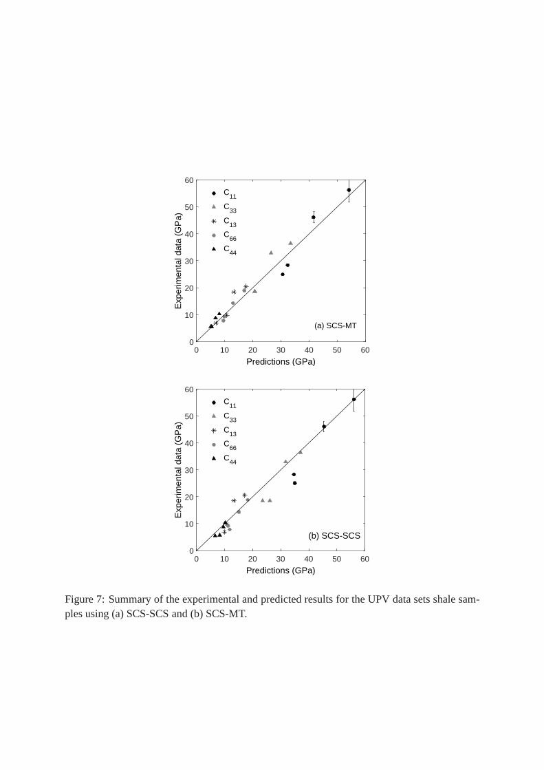
the most common non-clay mineral in shales. Figure 7 illustrates the predicted and the experi-368

mental results of the elastic constants of transversely isotropic shales using both SCS-SCS and369

SCS-MT strategies with bars showing the experimental standard deviation for each constant.370

The values of these constants, Thomsen’s anisotropy parameters ofε = (C11 − C33)/2C33 and371

γ = (C66 − C44)/2C44 and their relative errors (%) are also given in Tables 6 and 7.372

Comparing the relative errors between two up-scaling strategies revealed that there is no373

clear superiority for one strategy over the other one. This result can be justified due to the374

fact that each component of the stiffness tensor is a combination of two elastic constants, for375

example for an isotropic materialC11 = E(1 − ν)/((1 + ν)(1 − 2ν)) . As it was highlighted376

in Section 2, numerical studies using SCS and MT schemes for predicting homogenised elastic377

response of matrix-inclusion morphology showed that each of this elastic constant can be better378

predicted with one of these schemes (Goodarzi et al. 2016). In fact, the error observed in379

homogenised stiffness tensor components can be seen as the combined error of homogenised380

elastic constants. It can be observed that both SCS-SCS and SCS-MT methods produce some381

theoretical errors. However, in general, it can be concluded that SCS-SCS performed slightly382

better, particularly in terms of capturing anisotropy.383

Table 6: Experimental (Exp) and predicted (Pred) elastic constants for the UPV data sets sam-ples using SCS-SCS.

Elastic Kimmeridge Jurassic Woodford-2 Woodford-2constant Shale Shale Shale Shale

Exp. Pred. Error Exp. Pred. Error Exp. Pred. Error Exp. Pred. Error(%) (%) (%) (%)

C11 (GPa) 56.2 56 0.35 46.1 45.3 1.73 25 35 40 28.3 34.6 22.2C33 (GPa) 36.4 37 1.64 32.9 31.7 3.64 18.6 26 39.7 18.6 23.5 26.C13 (GPa) 20.5 17.2 16.1 18.5 13.3 28.1 6.9 9.96 44.3 9.8 10.6 8.16C66 (GPa) 18.9 18.2 3.70 14.3 15 4.9 7.8 11.8 51.2 9.3 11.1 19.3C44 (GPa) 10.3 10.2 0.97 8.8 9.5 7.95 5.7 8.2 43.8 5.5 6.6 20

ε 0.27 0.26 5.5 0.2 0.21 6.9 0.17 0.17 0.0 0.26 0.23 9.4γ 0.41 0.39 6.0 0.31 0.29 7.3 0.18 0.21 19 0.34 0.34 0.0

Table 7: Experimental (Exp) and predicted (Pred) elastic constants for the UPV data sets sam-ples using SCS-SCS.

Elastic Kimmeridge Jurassic Woodford-2 Woodford-2constant Shale Shale Shale Shale

Exp. Pred. Error Exp. Pred. Error Exp. Pred. Error Exp. Pred. Error(%) (%) (%) (%)

C11 (GPa) 56.2 54.2 3.55 46.1 41.6 9.76 25 30.6 22.4 28.3 32.5 14.8C33 (GPa) 36.4 33.5 8 32.9 26.4 19.7 18.6 20.6 10.7 18.6 20.7 11.2C13 (GPa) 20.5 17.6 14.1 18.5 13.3 28.1 6.9 10.1 46.3 9.8 10.8 10.2C66 (GPa) 18.9 17 10 14.3 13 9.1 7.8 9.5 21.7 9.3 9.9 6.45C44 (GPa) 10.3 8.1 21.3 8.8 6.7 23.8 5.7 5.4 5.26 5.5 5.1 7.3

ε 0.27 0.31 0.13 0.2 0.28 43.5 0.17 0.24 41 0.26 0.28 9.3γ 0.41 0.54 31.5 0.31 0.47 50.4 0.18 0.37 106 0.34 0.47 36.2

The prediction errors are relatively lower for the elastic constantsC11 andC33 compared384

to those forC13. This can be explained by the high degree of measurement uncertainties in385

C13 where the standard deviations are usually expected to be between 30% and 50% (Jones386

and Wang 1981; Domnesteanu, McCann and Sothcott 2002; Jakobsen and Johansen 2000).387

Additionally, Sayers (2013a) studied the anisotropic response of shales and concluded that the388

value ofC13 can be affected by features such as the presence of microcracks in the sample,389

which is ignored in our model. Considering the complexity ofshale microstructure in addition390

to the high standard deviations which are usually observed when measuring shale properties,391

we conclude that the homogenisation methods can provide valuable mechanical results simply392

and inexpensively, using just quantitative mineralogicaldescriptions of shales.393

The data in Table 7 show that the anisotropy was captured verywell for all the data sets.394

However, it is obvious that the absolute predicted elastic constants are not satisfactory for the395

case of Woodford shales in comparison with the results obtained for Kimmeridge and Jurassic396

shales. As the homogenisation overestimates the elastic modulus, this could be due to the lack397

of information on the confining pressures used in the Woodford data sets. This is a critical398

parameter in the UPV test results as it can reduce the effect of microcracks, which are not con-399

sidered in the modelling. For example, elevation in confining pressure from 5 MPa to 80 MPa400

increasesC11 by 40% in Jurassic shale (Hornby 1998). The TOC contents of these samples401

were not provided in the reference which could also have significantly reduced the elastic re-402

sponse. Moreover, it is also of interest to compare these results with previous micro-mechanical403

modelling of the same data sets. Jakobsen et al. (2003) attempted to predict the Jurassic shale404

elastic response. Several strategies were tried and the best results they could achieve were close405

to the measured properties at a confining pressure of 20 MPa. Vasin et al. (2013) started with406

a single clay particle to build up a shale model for Kimmeridge shale. They could not manage407

to reproduce the elastic response using the shale characterization obtained experimentally. By408

increasing the porosity to more than 10% with a specific aspect ratio, a good agreement was409

achieved with the predicted results and the measured elastic constant at a confining pressure410

of 80 MPa. It should be emphasised that the predicted data here are obtained solely using the411

shale characterisation presented in the literature (Hornby 1998; Sierra et al. 2010), without any412

further calibration.413

5.3 Indentation data sets414

5.3.1 Indentation test415

Indentation tests generate mechanical properties of materials from their surface response. In416

this test, an indenter with known mechanical properties is pushed into a material surface with417

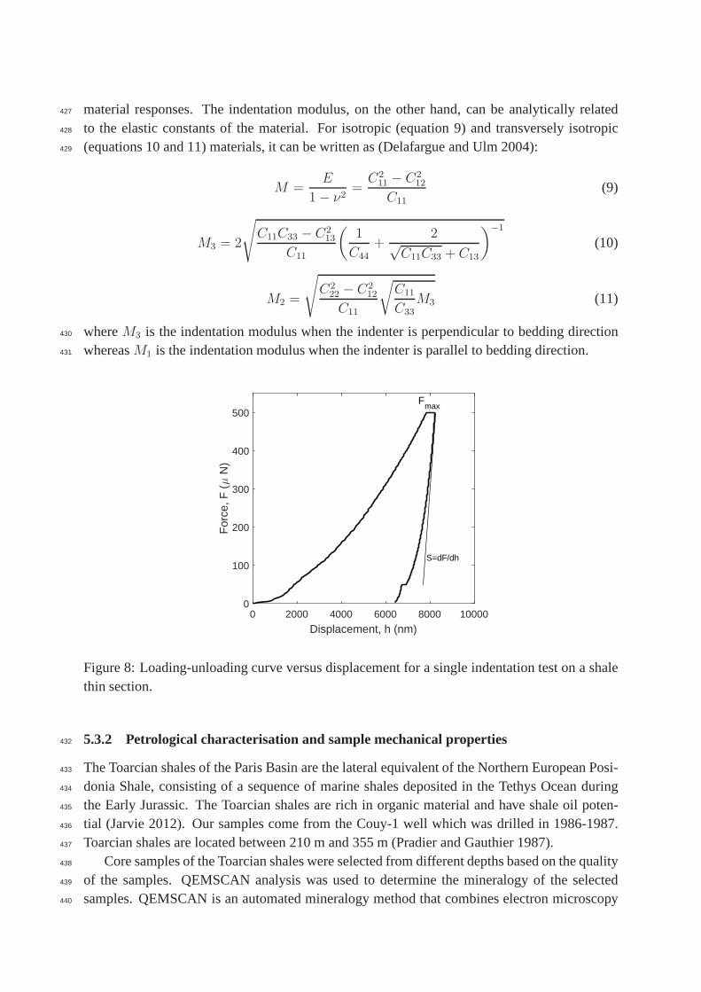
unknown properties. The continuous loading and unloading curves versus displacement are418

plotted as depicted in Figure 8, and two material propertiescan be defined as follows:419

H =Fmax

Ac

(7)

M =

√π

2

S√Ac

with S =

(

dF

dh

)

h=hmax

(8)

whereH is defined as the indentation hardness,M is the indentation modulus,Fmax is the420

maximum applied force on the indenter,hmax is the maximum penetration depth,Ac is the421

projected contact area on the sample, andS is the stiffness of the unloading curve athmax (see422

Figure 8).423

Indentation hardness is related to the elastic-plastic response of the material; however, it424

cannot be directly related to the conventional plastic parameters such as the angle of friction425

and cohesion. Therefore, this mechanical property is mainly derived for comparison of different426

Predictions (GPa)0 10 20 30 40 50 60

Exp

erim

enta

l dat

a (G

Pa)

0

10

20

30

40

50

60

(a) SCS-MT

C11

C33

C13

C66

C44

Predictions (GPa)0 10 20 30 40 50 60

Exp

erim

enta

l dat

a (G

Pa)

0

10

20

30

40

50

60

(b) SCS-SCS

C11

C33

C13

C66

C44

Figure 7: Summary of the experimental and predicted resultsfor the UPV data sets shale sam-ples using (a) SCS-SCS and (b) SCS-MT.

material responses. The indentation modulus, on the other hand, can be analytically related427

to the elastic constants of the material. For isotropic (equation 9) and transversely isotropic428

(equations 10 and 11) materials, it can be written as (Delafargue and Ulm 2004):429

M =E

1− ν2=

C2

11− C2

12

C11

(9)

M3 = 2

√

C11C33 − C213

C11

(

1

C44

+2√

C11C33 + C13

)

−1

(10)

M2 =

√

C222− C2

12

C11

√

C11

C33

M3 (11)

whereM3 is the indentation modulus when the indenter is perpendicular to bedding direction430

whereasM1 is the indentation modulus when the indenter is parallel to bedding direction.431

Displacement, h (nm)0 2000 4000 6000 8000 10000

For

ce, F

(µ

N)

0

100

200

300

400

500F

max

S=dF/dh

Figure 8: Loading-unloading curve versus displacement fora single indentation test on a shalethin section.

5.3.2 Petrological characterisation and sample mechanical properties432

The Toarcian shales of the Paris Basin are the lateral equivalent of the Northern European Posi-433

donia Shale, consisting of a sequence of marine shales deposited in the Tethys Ocean during434

the Early Jurassic. The Toarcian shales are rich in organic material and have shale oil poten-435

tial (Jarvie 2012). Our samples come from the Couy-1 well which was drilled in 1986-1987.436

Toarcian shales are located between 210 m and 355 m (Pradier and Gauthier 1987).437

Core samples of the Toarcian shales were selected from different depths based on the quality438

of the samples. QEMSCAN analysis was used to determine the mineralogy of the selected439

samples. QEMSCAN is an automated mineralogy method that combines electron microscopy440

with energy dispersive spectroscopy for quantitative mineralogical analysis of rock sample.441

Based on the mineralogical data, four samples were selectedfor indentation measurements to442

determine the mechanical properties. Figure 9 shows digital mineralogical image generated443

by QEMSCAN analysis. Table 8 provides information about thetotal organic carbon,Tmax444

index and mineralogical descriptions for the samples used in indentation tests. The following445

empirical relationship has been used to convert the TOC in weight percent to kerogen in volume446

percent (Vernik and Nur 1992; Carcione 2000):447

Kr =TOCρb0.75ρk

(12)

whereρb is the bulk density of the sample,ρk is the kerogen density andKr is the volumetric448

kerogen content. The values ofTmax are less than 435 indicating that the shale samples are449

immature; therefore, a value of 1.25 g/cm3 was selected for the kerogen density (Okiongbo,450

Aplin and Larter 2005).451

1 mm

Figure 9: QEMSCAN image based on combination of SEM and EDS digital images.

For each shale sample two surfaces, one parallel and one perpendicular to bedding, were pre-452

pared and polished in order to provide relatively smooth area as for the PeakForce QNMr tests.453

Tests were performed using the Berkovich indenter along with a force-controlled condition with454

a maximum value of 400 mN set for all experiments. This maximum possible load was applied455

in order to create the maximum possible contact area and to obtain the best surface response of456

the whole shale composite. This force value generated indentation depths from 3.5µm to 6.5457

µm, depending on the sample stiffness.458

Due to the complex nature of shale, even at the scale of a few microns, a large number of459

indents must be conducted in order to obtain a robust statistical description of the mechanical460

response. Here, an average, around 80 indentations were conducted on each surface to char-461

acterise its mechanical response. It should be noted that the indentation data usually contains462

some out-of-range values which might be caused by the indenter mainly touching a large stiff463

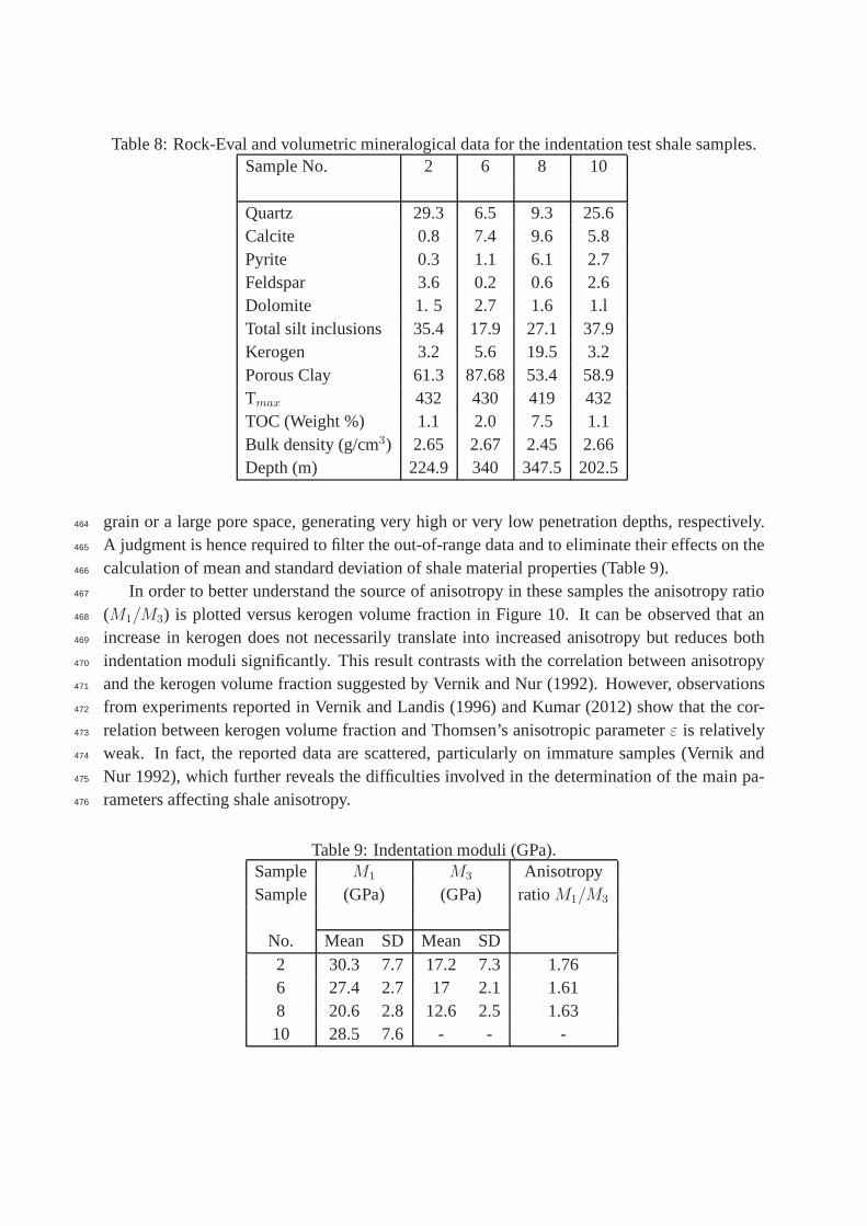
Table 8: Rock-Eval and volumetric mineralogical data for the indentation test shale samples.Sample No. 2 6 8 10

Quartz 29.3 6.5 9.3 25.6Calcite 0.8 7.4 9.6 5.8Pyrite 0.3 1.1 6.1 2.7Feldspar 3.6 0.2 0.6 2.6Dolomite 1. 5 2.7 1.6 1.lTotal silt inclusions 35.4 17.9 27.1 37.9Kerogen 3.2 5.6 19.5 3.2Porous Clay 61.3 87.68 53.4 58.9Tmax 432 430 419 432TOC (Weight %) 1.1 2.0 7.5 1.1Bulk density (g/cm3) 2.65 2.67 2.45 2.66Depth (m) 224.9 340 347.5 202.5

grain or a large pore space, generating very high or very low penetration depths, respectively.464

A judgment is hence required to filter the out-of-range data and to eliminate their effects on the465

calculation of mean and standard deviation of shale material properties (Table 9).466

In order to better understand the source of anisotropy in these samples the anisotropy ratio467

(M1/M3) is plotted versus kerogen volume fraction in Figure 10. It can be observed that an468

increase in kerogen does not necessarily translate into increased anisotropy but reduces both469

indentation moduli significantly. This result contrasts with the correlation between anisotropy470

and the kerogen volume fraction suggested by Vernik and Nur (1992). However, observations471

from experiments reported in Vernik and Landis (1996) and Kumar (2012) show that the cor-472

relation between kerogen volume fraction and Thomsen’s anisotropic parameterε is relatively473

weak. In fact, the reported data are scattered, particularly on immature samples (Vernik and474

Nur 1992), which further reveals the difficulties involved in the determination of the main pa-475

rameters affecting shale anisotropy.476

Table 9: Indentation moduli (GPa).Sample M1 M3 AnisotropySample (GPa) (GPa) ratioM1/M3

No. Mean SD Mean SD2 30.3 7.7 17.2 7.3 1.766 27.4 2.7 17 2.1 1.618 20.6 2.8 12.6 2.5 1.6310 28.5 7.6 - - -

Kerogen (Vol %)0 5 10 15 20

Ani

sotr

opy

ratio

(M

1/M3)

1.5

1.55

1.6

1.65

1.7

1.75

1.8

35.43

17.9227.1

Figure 10: Anisotropy versus kerogen volume fraction (datalabel is the volume fraction of siltinclusions).

5.3.3 Homogenisation of organic-rich shales477

In order to calculate the indentation moduli from the homogenisation technique, porosity and478

organic matter content should also be taken into account, inaddition to the mineralogical data479

provided in Table 8. Here, an estimation of the porosity is required as this parameter was not480

measured. In addition, identifying the material properties of organic matter and its role on the481

overall mechanical behaviour of the shale composite is alsoimportant.482

Due to the fact that all the samples have been retrieved from similar depths (see Table 8),483

it is assumed that the clay packing density,η , is the same in all samples. The clay packing484

density relates to the compaction state of clay particles and can be defined as:η = 1 − φclay.485

This value can be back-calculated from one data set by equalising the experimental value to the486

predicted one. The obtained value is then used as the ‘reference parameter’ for the rest of the487

experimental data. In addition, as the sample had been exposed to room-temperature for a long488

time before the test, the shale will be considered as dry, with no fluid within the pore spaces.489

An assumption in the homogenisation formulation is that thematrix is considered as a con-490

tinuous phase and the inclusions are isolated and fully surrounded by the matrix phase. SEM491

observations (see Figure 3) suggest that the organic matteris a semi-continuous phase mixed492

with the porous clay. We therefore assume that the organic matter can be considered to be493

part of the shale matrix so that its contribution is taken into account, along with that of the494

porosity, in the first level of homogenisation. Previous approaches include considering organic495

matter as the background phase in shale (Vernik and Landis 1996, Bayuk et al. 2008; Sayers496

2013b), combining kerogen and solid clay as the elementary building block of the shale matrix,497

or adding kerogen as inclusions (Guo et al. 2014).498

Based on the observation that kerogen in the tested samples does not increase the anisotropy499

ratio, it is assumed here that kerogen is mixed with a porous clay having the same packing500

density in all the samples. The combination of these phases through the use of SCS enables us to501

reproduce a system of semi-continuous random pore and kerogen networks with no preferential502

orientation. This approach is consistent with the experimental observation (Figure 10) in which503

anisotropy is slightly reduced by an increase in kerogen. The mechanical properties of kerogen504

are an important and controversial factor in the predictionof the overall mechanical response505

for organic-rich shale. However, as discussed in Section 3,there is a discrepancy between506

the reported elastic properties of kerogen in the literature. In Section 4, the nanoscale direct507

mechanical measurements were conducted on an immature shale sample which provided a mean508

value of 6 GPa for kerogen assuming that the Poisson’s ratio is 0.3. As the current samples are509

also immature, this value will be adopted for the micromechanical modelling.510

Based on the predicted results in Section 5.2, the SCS homogenisation strategy was also511

considered at the second level. The clay packing density wascalibrated to be approximately512

0.75 based on the indentation modulus parallel to the bedding direction (M1) for sample No. 2.513

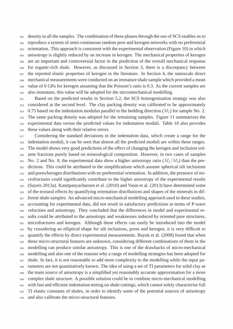
The same packing density was adopted for the remaining samples. Figure 11 summarizes the514

experimental data versus the predicted values for indentation moduli. Table 10 also provides515

these values along with their relative errors.516

Considering the standard deviations in the indentation data, which create a range for the517

indentation moduli, it can be seen that almost all the predicted moduli are within these ranges.518

The model shows very good predictions of the effect of changing the kerogen and inclusion vol-519

ume fractions purely based on mineralogical composition. However, in two cases of samples520

No. 2 and No. 8, the experimental data show a higher anisotropy ratio (M1/M3) than the pre-521

dictions. This could be attributed to the simplifications which assume spherical silt inclusions522

and pores/kerogen distributions with no preferential orientation. In addition, the presence of mi-523

crofractures could significantly contribute to the higher anisotropy of the experimental results524

(Sayers 2013a). Kanitpanyacharoen et al. (2010) and Vasin et al. (2013) have determined some525

of the textural effects by quantifying orientation distributions and shapes of the minerals in dif-526

ferent shale samples. An advanced micro-mechanical modelling approach used in these studies,527

accounting for experimental data, did not result in satisfactory predictions in terms of P-wave528

velocities and anisotropy. They concluded that the differences in model and experimental re-529

sults could be attributed to the anisotropy and weaknesses induced by oriented pore structures,530

microfractures and kerogen. Although these effects can easily be introduced into the model531

by considering an elliptical shape for silt inclusions, pores and kerogen, it is very difficult to532

quantify the effects by direct experimental measurements.Bayuk et al. (2008) found that when533

these micro-structural features are unknown, consideringdifferent combinations of them in the534

modelling can produce similar anisotropy. This is one of thedrawbacks of micro-mechanical535

modelling and also one of the reasons why a range of modellingstrategies has been adopted for536

shale. In fact, it is not reasonable to add more complexity tothe modelling while the input pa-537

rameters are not quantitatively known. The idea of using a set of TI parameters for solid clay as538

the main source of anisotropy is a simplified yet reasonably accurate approximation for a more539

complex shale structure. A possible solution could be to combine micro-mechanical modelling540

with fast and efficient indentation testing on shale cuttings, which cannot solely characterise full541

TI elastic constants of shales, in order to identify some of the potential sources of anisotropy542

and also calibrate the micro-structural features.543

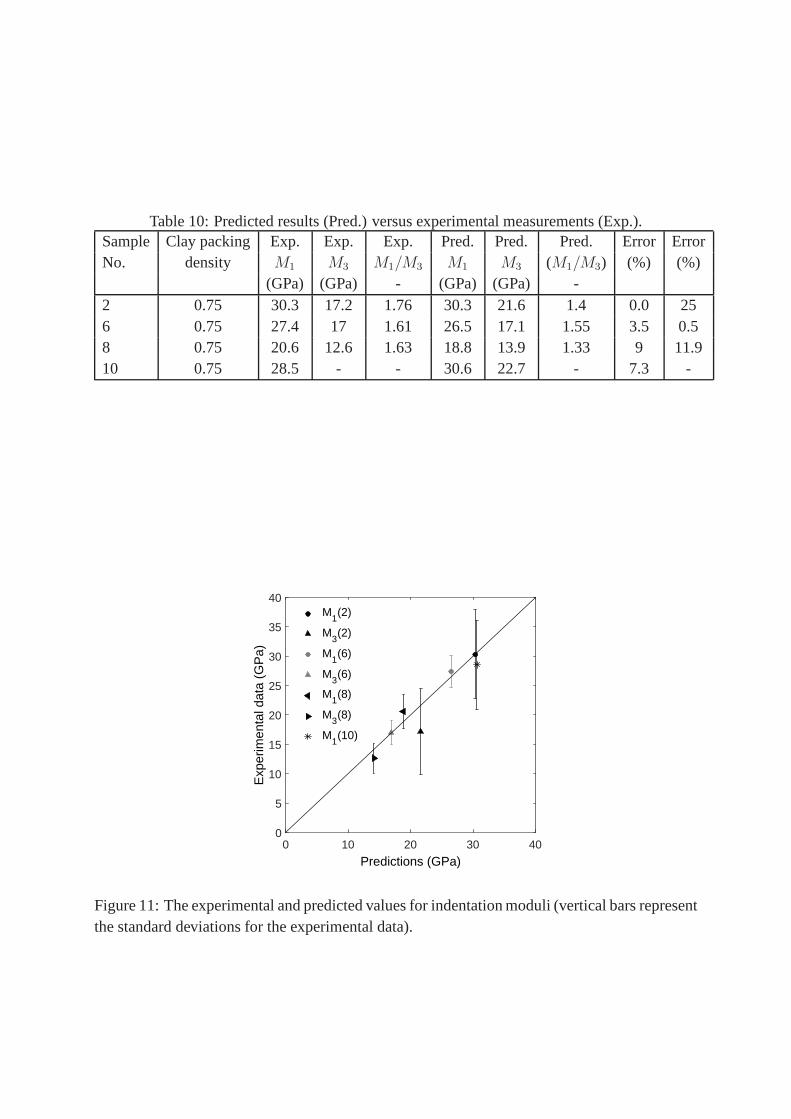
Table 10: Predicted results (Pred.) versus experimental measurements (Exp.).Sample Clay packing Exp. Exp. Exp. Pred. Pred. Pred. Error ErrorNo. density M1 M3 M1/M3 M1 M3 (M1/M3) (%) (%)

(GPa) (GPa) - (GPa) (GPa) -2 0.75 30.3 17.2 1.76 30.3 21.6 1.4 0.0 256 0.75 27.4 17 1.61 26.5 17.1 1.55 3.5 0.58 0.75 20.6 12.6 1.63 18.8 13.9 1.33 9 11.910 0.75 28.5 - - 30.6 22.7 - 7.3 -

Predictions (GPa)0 10 20 30 40

Exp

erim

enta

l dat

a (G

Pa)

0

5

10

15

20

25

30

35

40M

1(2)

M3(2)

M1(6)

M3(6)

M1(8)

M3(8)

M1(10)

Figure 11: The experimental and predicted values for indentation moduli (vertical bars representthe standard deviations for the experimental data).

6 Conclusions544

We have studied the capabilities of a range of multi-scale homogenisation techniques to model545

and predict the elastic response of shales. The shales were assumed to be a composite formed546

by a matrix containing solid clay, kerogen and pores. Solid mineral grains/inclusions were ran-547

domly distributed within the matrix. Consequently, two levels of homogenisation were required548

involving the SCS method at the first level to upscale the shale matrix and, at the second level,549

the capabilities of both MT and SCS in homogenising the matrix-inclusion morphology.550

Resulting Young’s modulus maps using the AFM-based PeakForce QNMr mechanical char-551

acterisation mode on two sections of immature, organic-rich shale, showed an isotropic response552

for quartz grains. The porous clay, in contrast, showed highly anisotropic behaviour with al-553

most the same anisotropy ratio as measured at the macroscale. Organic matter is seen to be a554

semi-continuous phase within the porous clay matrix, with ameasured Young’s modulus of 6555

GPa.556

Results from the homogenization method were evaluated against the limited geomechanical557

datasets available in the literature. Considering the multiscale complexity of shales and also558

the high standard deviations usually obtained in mechanical experiments on shale samples,559

the values estimated by the homogenisation method, which are based solely on mineralogical560

descriptions, provide valuable predictions of the mechanical response. Additionally, comparing561

SCS and MT for the second level of homogenisation, it was concluded that SCS produced a562

slightly better prediction of elastic response with a very good estimate of anisotropy.563

Finally, to generate more data for organic-rich shales easily and inexpensively, advanced564

indentation tests were implemented. Based on the observations in the nanoscale mechanical565

maps, organic matter was taken into account in the first levelof homogenization with the elastic566

modulus being measured by nano-mechanical mapping. A comparison between the predicted567

indentation moduli and the experimental values confirms thecapability of the multi-scale ho-568

mogenization method to predict the effect of kerogen on the elastic response of shales, provided569

that this phase is suitably accounted for. However, micro-structural features such as grain shape570

or pore aspect ratio, which cannot be measured directly, need to be calibrated in order to further571

adjust the predicted anisotropy. This calibration can be performed with indentation data sets572

which can be obtained from shale cuttings. Generally, it canbe concluded that the homogeniza-573

tion technique can be effectively used as an auxiliary approach to conventional rock mechanics574

tests to estimate the elastic response of shale rocks using petrological and mechanical properties575

of shale cuttings.576

Acknowledgements577

The authors would like to acknowledge the collaboration of the BRGM (the French geo-578

logical survey) and SGS Horizon B.V. by providing shale samples characterisation and the ex-579

perimental indentation data. The first author greatly acknowledges discussions with Mr. Leon580

Bowen on sample preparation, SEM and EDS analyses. We also thank Dr. Richard Thompson581

for providing access to the AFM facilities at Durham University.582

Rerefences583

Amirmajdi O.M., Ashyer-Soltani R., Clode M.P., Mannan S.H., Wang Y., Cabruja E. and Pel-584

legrini G. 2009. Cross-section preparation for solder joints and MEMS device using argon ion585

beam milling.IEEE Transactions on electronics packaging manufacturing32(4), 265-271.586

Antonangeli D., Krish M., Fiquet G., Badro J., Farber D.L., Bossak A. and Merkel S. 2005.587

Aggregate and single-crystalline elasticity of hcp cobaltat high pressure.Physical Review B588

72, 134303.589

Aplin A.C. and Macquaker J.H.S. 2011. Mudstone diversity: origin and implications for source,590

seal and reservoir properties in petroleum systems.The American Association of Petroleum591

Geologists (AAPG) Bulletin95(12), 2031-2059.592

Bass J.D. 1995. Elasticity of minerals, glasses, and melts.In: Minerals Physics & Crystallog-593

raphy: A handbook of physical constants(ed. T.J. Ahrens), pp. 45-63.AGU Reference Shelf.594

ISBN 9780875908526.595

Bayuk I.O., Ammerman M. and Chesnokov E.M. 2008. Upscaling of elastic properties of596

anisotropic sedimentary rocks.Geophysical Journal International172, 842-860.597

Bobko C. and Ulm F.J. 2008. The nano-mechanical morphology of shale.Mechanics of Mate-598

rials 40, 318-337.599

Bruker’s Application Note#141. Toward quantitative nanomechanical measurements on live600

cells with PeakForce QNM. https://www.bruker.com/products.601

Bruker’s Application Note#128. Quantitative mechanical property mapping at the nanoscale602

with PeakForce QNM. https://www.bruker.com/products.603

Carcione J.M. 2000. A model for seismic velocity and attenuation in petroleum source rocks.604

Geophysics65(4), 1080-1092605

Chalmers G.R., Bustin R.M. and Power I.M. 2012. Characterization of gas shale pore systems606

by porosimetry, pycnometry, surface area, and field emission scanning electron microscopy/transmission607

electron microscopy image analyses: Examples from the Barnett, Woodford, Haynesville, Mar-608

cellus and Doig units.The American Association of Petroleum Geologists (AAPG)96(6), 1099-609

1119.610

Delafargue A. and Ulm F.J. 2004. Explicit approximations ofthe indentation modulus of elas-611

tically orthotropic solids for conical indenters.International Journal of Solids and Structures612

41, 7351-7360.613

Domnesteanu P., McCann C. and Sothcott J. 2002. Velocity anisotropy and attenuation of shale614

in under- and over pressured conditions.Geophysical Prospecting50, 487-503.615

Draege A., Jakobsen M. and Johansen T.A. 2006. Rock physics modelling of shale diagenesis.616

Petroleum Geoscience12, 49-57.617

Eliyahua M., Emmanuel S., Day-Stirrat R.J. and Macaulay C.I. 2015. Mechanical properties618

of organic matter in shales mapped at the nanometer scale.Marine and Petroleum Geology59,619

294-304.620

Fritsch A. and Hellmich C. 2007. Universal microstructuralpatterns in cortical and trabecular,621

extracellular and extravascular bone materials: Micromechanics-based prediction of anisotropic622

elasticity.Journal of Theoretical Biology244, 597-620.623

Goodarzi M., Rouainia M. and Aplin A.C. 2016. Evaluation of multi-scale homogenisation624

methods for the case of clayey rock elastic properties usingnumerical simulation.Computa-625

tional Geosciences1-14, doi:10.1007/s10596-016-9579-y626

Guo Z.Q., Li X.Y. and Liu C. 2014. Anisotropy parameters estimate and rock physics analysis627

for the Barnett Shale.Journal of Geophysics and Engineering11, 065006.628

Heyliger P., Ledbetter H. and Kim S. 2003. Elastic constantsof natural quartz.The Journal of629

the Acoustical Society of America114, 644-650.630

Hill R. 1965. A self-consistent mechanics of composite materials. Journal of Mechanics and631

Physics of Solids13, 213-222.632

Hornby B.E., Schwartz L. and Hudson J. 1994. Anisotropic effective medium modelling of the633

elastic properties of shales.Geophysics59, 1570-83.634

Hornby B.E. 1998. Experimental laboratory determination of the dynamic elastic properties of635

wet, drained shales.Journal of Geophysical Research103(B12), 29945-29964.636

Jakobsen M. and Johansen T.A. 2000. Anisotropic approximations for mudrocks: A seismic637

laboratory study.Geophysics65(6), 1711-1725.638

Jakobsen M., Hudson J.A. and Johansen T.A. 2003. T-matrix approach to shale acoustics.639

Geophysical Journal International154, 533-558640

Jarvie D.M. 2012. Shale resource systems for oil and gas: Part 2 Shale-oil resource systems.641

In: Shale reservoirs Giant resources for the 21st century(ed. J.A. Breyer), pp. 89-119. AAPG642

Memoir Volume97. ISBN 978-1-62981-011-9.643

Jones L.E.A. and Wang H.F. 1981. Ultrasonic velocities in Cretaceous shales from the Williston644

basin.Geophysics46(3), 288-297.645

Kanitpanyacharoen W., Wenk H.R., Kets F., Lehr C. and Wirth R. 2011. Texture and anisotropy646

analysis of Qusaiba shales.Geophysical Prospecting59, 536-556.647

Klusemann B., Bohm H.J. and Svendsen B. 2012. Homogenisation methods for multi-phase648

elastic composites with non-elliptical reinforcements: Comparisons and benchmarks.European649

Journal of Mechanics - A/Solids34, 21-37.650

Kumar V., Sondergeld C.H. and Rai C.H. 2012. Nano to macro mechanical characterization651

of shale. SPE Annual Technical Conference and Exhibition, San Antonio, Texas, USA. SPE652

159804.653

Kumar V. 2012. Geomechanical Characterization of Shale Using Nano-indentation. MSc dis-654

sertation, University of Oklahoma.655

Laws N. 1977. The determination of stress and strain concentrations at an ellipsoidal inclusion656

in an anisotropic material.Journal of Elasticity7(1), 91-97.657

Mavko G., Mukerji T. and Dvorkin J. 2009. The Rock Physics Handbook. Cambridge Univer-658

sity Press. ISBN 9780521861366.659

Mori T. and Tanaka K. 1973. Average stress in matrix and average elastic energy of materials660

with misfitting inclusions.Acta Metallurgica21, 571-574.661

Mortazavi B., Baniassadi M,. Bardon J. and Ahzi S. 2013. Modelling of two-phase random662

composite materials by finite element, Mori-Tanaka and strong contrast methods.Composites:663

Part B45, 1117-1125.664

Okiongbo K.S., Aplin A.C. and Larter S.R. 2005. Changes in Type II Kerogen Density as a665

Function of Maturity: Evidence from the Kimmeridge Clay Formation. Energy & Fuels19,666

2495-2499.667

Ortega J.A., Ulm F.J. and Abousleiman Y. 2007. The effect of the nanogranular nature of shale668

on their poroelastic behaviour.Acta Geotechnica2, 155-182.669

Ortega J.A., Ulm F.J. and Abousleiman Y. 2010. The effect of particle shape and grain-scale670

properties of shale: A micromechanics approach.International Journal of Numerical and Ana-671

lytical Method in Geomechanics34, 1124-1156.672

Peng S., Yang J., Xiao X., Loucks B., Ruppel S. and Zhang T. 2015. An integrated method673

for upscaling pore-network characterization and permeability estimation: example from the674

Mississippian Barnett shale.Transport in Porous Media109, 359-376.675

Pradier B. and Gauthier B. 1987. Etude preliminaire de la matiere organique sedimentaire. In:676

Geologie profonde de la France, forage scientifique de Sancerre-Couy(ed. C. Lorenz), pp.677

103-108. Documents no135 du Bureau de Recherches Geologiques et Minieres (BRGM). in678

French679

Qin X., Han D. and Zhao L. 2014. Rock physics modeling of organic-rich shales with different680

maturity levels.SEG Technical Program Expanded Abstracts, 2952-2957.681

Sayers C.M. 1994. The elastic anisotropy of shales.Journal of Geophysical Research99(B1),682

767-774.683

Sayers C.M. 2013a. The effect of anisotropy on the Young’s moduli and Poisson’s ratios of684

shales.Geophysical Prospecting61, 416-426.685

Sayers C.M. 2013b. The effect of kerogen on the elastic anisotropy of organic-rich shales.686

Geophysics78, (2), D65-D74.687

Sierra R., Tran M.H., Abousleiman Y.N. and Slatt R.M. 2010. Woodford Shale Mechanical688

Properties and the Impacts of Lithofacies. The 44th US Rock Mechanics Symposium and 5th689

US-Canada Rock Mechanics Symposium. Salt Lake City ARMA-10-461690

Trtik P., Kaufmann J. and Volz U. 2012. On the use of peak-force tapping atomic force mi-691

croscopy for quantification of the local elastic modulus in hardened cement paste.Cement and692

Concrete Research42, 215-221.693

Ulm F.J. and Abousleiman Y. 2006. The nanogranular nature ofshale. Acta Geotechnica1,694

77-88.695

Vasin R.N., Wenk H.R., Kanitpanyacharoen W., Matthies S. and Wirth R. 2013. Elastic anisotropy696

modeling of Kimmeridge shale.Journal of Geophysical Research: Solid Earth118, 3931-3956.697

Vernik L. and Nur A. 1992. Ultrasonic velocity and anisotropy of hydrocarbon source rocks.698

Geophysics57, 727-735.699

Vernik L. and Landis C. 1996. Elastic anisotropy of source rocks: Implication for HC generation700

and primary migration.AAPG Bulletin80, 531-544.701

Vernik L. and Milovac J. 2011. Rock physics of organic shales. The Leading Edge30, 318-323.702

Wang Z., Wang H. and Cates M.E. 2001. Effective elastic properties of solid clays.Geophysics703

66(2), 428-440.704

Whitaker M.L., Liu W., Wang L. and Li B. 2010. Acoustic velocities and elastic properties of705

Pyrite (FeS2) to 9.6 GPa.Journal of Earth Science21, 792-800.706

Wu X., Chapman M., Li X.Y. and Dai H. 2012. Anisotropic elastic modelling for organic shales.707

74th EAGE Conference and Exhibition SPE EUROPE, Copenhagen, Denmark, P314708

Yan F. and Han D. 2013. Measurement of elastic properties of kerogen. 83rd SEG Annual709

Meeting, Houston, USA, Expanded Abstracts, 2778-2782710

Zargari S., Prasad M., Mba K.C. and Mattson E.D. 2013. Organic maturity, elastic properties,711

and textural characteristics of self-resourcing reservoirs. Geophysics78(4), D223-D235.712

Zeszotarski J.C., Chromik R.R., Vinci R.P., Messmer M.C., Michels R. and Larsen J.W. 2004.713

Imaging and mechanical property measurements of kerogen via nanoindentation.Geochimica714

et Cosmochimica Acta68, 4113-4119.715

Zhu Y., Xu S., Payne M., Martinez A., Liu E., Harris C. and Bandyopadhyay K. 2012. Improved716

rock-physics model for shale gas reservoirs. 82nd SEG Meeting, Denver, USA, Expanded717

Abstracts 2952-2957.718

Zu Y., Xu S., Liu E., Payne M.A. and Terrell M.J. 2013. Predicting anisotropic source rock719

properties from well data: U.S. Patent 2013/0013209 A1.720