Page 1 of 22

Golden Ratio Axioms of Time and Space.

Stephen H. Jarvis.

GRAVIELECTRIC, Stephen.jarvis@gravielectric.com, www.gravielectric.com

Tel: 61-2-99221289

Abstract: This sequel to “Gravity’s Emergence from Electrodynamics” will more closely examine the process of

time as the Golden Ratio equation when applied to space, more than developing electrodynamic wavefunction

equations, but setting an axiomatic base for the Golden Ratio as time when applied to space. Through this process

we shall derive 𝜋, the fine structure constant, and the speed of light, while also confirming through these

independent equations the idea of the Uncertainty Principle and Quantum Entanglement. More specifically, three

fundamental things to be demonstrated here using the Golden Ratio algorithm of time will be deriving the dipole of

magnetism, the electrical monopole field, and their relation to the Golden Ratio in creating the basis for the Fine

Structure Constant, charge of the electron, the speed of light, and the subatomic multi-traits of the elementary

particles. In confirming the need to explain the reason for the upgraded axioms for time and space, a general

criticism of contemporary physics’ current use of space and time and its limitation given the entirely hypothetical

nature of the resultant cosmic modelling theory regarding a multiverse and its endless possibilities is presented.

The solution to this problem is explained using a more solid definition for time as the Golden Ratio, more thoroughly

presented here in the context of the initial paper “Gravity’s Emergence from Electrodynamics” [1]; the first paper

was a general overview of the new a-priori for time, while this second paper examines all the generalisations and

assumptions presented in the first paper, reaching ultimate theoretical axioms for time in the context of space.

Keywords: golden ratio; time; space; electron; proton; neutron; electricity; magnetism; electromagnetism; fine

structure constant; pi; electrodynamics; elementary particle; subatomic particle; Higgs particle; quantum

entanglement; uncertainty principle; Rydberg equation; Brownian motion; fractal; electron shell; multiverse; big

bang; cosmology; Planck scale; speed of light; consciousness; cosmology

In the first paper “Gravity’s Emergence from Electrodynamics” [1] the idea of applying a new algorithm to

“time” was addressed. Subsequently it was demonstrated how this new algorithm could be utilised in the general

equations for electromagnetism and gravity, together with electron-shell modelling. In this paper, we will dive a step

deeper into the space and time structure of the golden ratio [2], highlighting why there are three spatial dimensions,

why the fine structure constant [3] is the value it is, why the speed of light is what it is [4], and why in space and

time there is the perfection of a circle via 𝜋 [5], all very fundamental constructs that we should not assume via

measured observations; science in the absence of a theory of everything is at best a process of “measuring”

features of space and time and formulating theories as to how each of these measurements relate with each other.

Here we will be diving within the idea of measuring by using the golden ratio for time alone. First, we shall explain

why we need this review of the current a-priori for space and time.

Page 2 of 22

1. The a-priori opportunity physics has yet to address.

Physics is “knowledge of nature” [6]. It involves the study of matter and its motion and behavior through

space and time, including concepts such as energy and force, while endeavoring to deliver an understanding of the

universe. As a discipline, it employs the scientific method [7] to test the validity of a physical theory by using a

methodical approach of experiment and research to test the theoretical proposals thereof. Much of what we know

of physics started with basic measurements of observable phenomena, measurements to find the mechanism and

associated predictability of those events in nature. Theories then developed to join these basic dots; initially we

applied rulers to measure distances between objects, and dials to measure time through the varying shades of

celestial rotations. Space [8] took on the definition of three dimensions, while time [9] was left as “something that a

clock measures”. And there’s our problem, “something that a clock measures”. If we are content with that definition,

then why not label space as “something that a ruler measures”? Let’s give more definition to time as per what was

presented in the first paper, “Gravity’s Emergence from Electrodynamics” [1], and apply this measurement of time

to space, such that space becomes “something that the golden ratio for time measures”. Presented here thus is a

new axiom for time that provides exactly that. The new axiom for time here cleans up much of scientific theory

regarding light/energy, mass, forces, and so on, everything that has embedded in it an equation for time. All those

predecessor concepts and associated equations will be supplemented with a more advanced understanding of

time, which paradoxically results in a cleaner and simpler description of all that physics aims to understand of space

and time.

One of the key flaws to physics today is where to go with cosmology [10]; a big bang [11], a steady state

[12], or the infinite multiverse [13]? What if the problem is how we register light to our perception? If the fundamental

basis of an idea is wrong, the development of that idea no matter how slightly incorrect will always result in unstable

theories unless the conclusions that result “require” an amendment to the fundamental idea the conclusions sprung

from. For if cosmology depends much on the fine structure behaviour of the atom, if our awareness of cosmology

is wrong, then so is the very fundamental basis we regard the atom. If our calculations though seem to be right,

the problems aren’t with our calculations, but how we perceive and in this case how we regard not space, but

“time”. The current trend in physics is to support the idea of an accelerating expanding universe and associated

cause being the big bang, the fundamental theoretical offspring of the red-shift of light. The argument presented

here is “what if light isn’t a singular dimensional entity entwined with space, yet an entity of its own with accelerating

expansive properties that provides the phenomena of entropy [14], spatial asymmetry [15], chirality [16], quantum

entanglement [17], and “all” the properties of energy, force, and motion? If such were the case, with that algorithm

physics should be far easier to understand space and time as a mathematics based on that algorithmic foundation

of time.

Conversely in the absence of this common start-point algorithm, physics has become vastly complex as

it seeks to explain space and time, reality, using numbers associated to equations/descriptors of tried and tested

phenomena, to link such phenomena with new equations and associated theories to arrive at an equation and

associated theory of everything on the Planck scale [18], a common end/start-point, to explain our origins and to

then maybe better understand our future purpose. Modern physics though, if it starts off on the wrong foot, wrong

a-priori, becomes a quagmire of ideas and equations never reaching their intended goal, ideas leading to false

conclusions that don’t add up in the far distant universe, ideas that make assumptions about new realities as the

only fix. This offering thus proposes a change to the current process of physics research with a new a-priori for

time and space. All the fragments of contemporary physics theory are nonetheless explained in the correct context

of a new axiomatic base for space and time, not as some may expect, but the explanation of the fundamental

tenets of space and time that makes all observed calculations in our natural world a logical and accurate inclusion.

Page 3 of 22

2. The solution.

The initial paper “Gravity’s Emergence from Electrodynamics” [1] was a general overview of the

fundamental reasoning behind gravity emerging from electrodynamics using the golden ratio as an algorithm for

time, detailing the two possible outcomes for each quantum step of determination of wavefunction expression of

light as “time” using the two results of the golden ratio equation, more specifically by provisionally labelling the

electrical component of electromagnetism to time-now, and the magnetic component to time-after, a starting point

nonetheless. For that paper merely proposed the idea of a sinusoidal wave for time “could” represent the dual

outcome consistent with the two results for the golden ratio for time ([1]; eq. 3,4). We didn’t prove time would be a

sinusoidal wave. We didn’t even demonstrate why space has three dimensions and why light emanates from a

point source in all directions in a 3-d space manifold. We also assumed two very fundamental constants, 𝜋 and the

fine structure constant, relying on measured research only. Here we shall provide the very key to unlocking the

fundamental basis for time as that sinusoidal algorithm in a 3-d spatial manifold, a sinusoidal curvature that imparts

itself such on 3-d space “in all axial directions”, and how this effect of light, although limited at a constant speed,

gives the effect of accelerating expansive 3-d space, and thus the illusion likewise of such a universe we would

consider to live in, together with deriving the value for 𝜋 in the context of fine structure constant of the atom. First,

we shall undertake a brief review of the new definitions for space and time from the first paper with a few additional

descriptors taking us to the sinusoidal wave construction.

Consider the following list of diagrams and equations from the first paper ([1]; figures 1-12, equations 1-

9). All the data contained in those equations and diagrams and associated descriptors are considered pre-required

for this discussion. In that set of equations and figures the overall outline for space and time was formed as a

golden ratio algorithm, provisionally labelling electricity and magnetism with time-now and time-after respectively,

establishing nonetheless with the general golden ratio equation how a basic link could be established between the

equations of gravity and electromagnetism, while detailing the process of atomic modelling and spatial dynamic

construction as per the derivation of the Rydberg formula ([1]; p13-15). It was thus considered that using the golden

ratio (as a time-algorithm) was successful in linking gravity with electromagnetism. Yet is this the “only” way to

achieve a link between the forces of gravity and electromagnetism together with the Rydberg formula [19]? Can

another algorithm, more complex, be used? Can another algorithm or first principle mechanism suggest other

possible “realities” including the one we are in, a type of basic multiverse-algorithm? To know this, we need to

examine more fundamentally the properties of time and space, such as “why” does space have three dimensions,

and why is the fine structure constant set at the value it is set at, and why does it require the use of “𝜋” in reference

to the wavelength of an electron, or as the initial paper [1] suggests, “time”? To answer these questions, we will

continue to investigate the use of the golden ratio for time given its success.

2.1 A closer look at the axioms for space and time

To consider a “moment”, as time not passing, it may as well be infinite time from the reference of another

process of time. Thus, obviously the definition of time here requires two references held in the same context of

laws of the flow of time. The initial paper presented time to represent the three basic equations: 𝑡𝐴 = 𝑡𝐵2 , 𝑡𝑁 = 1,

𝑡𝑁 = 𝑡𝐴 − 𝑡𝐵, ([1]; eq. 3, 4, 5), giving rise to 𝑡𝐴+ 𝑡𝐵

𝑡𝐴=

𝑡𝐴

𝑡𝐵 ([1]; eq. 6), providing two outcomes, two concepts, for time,

φ and −1

φ, as per the golden ratio. In short, the underlying premise was that time needs to be

relative to itself somehow to effect the idea of “flow”. The most basic mechanism we use is “before” and “after”, yet

as the initial paper [1] highlighted it is more complicated than this.

Page 4 of 22

In now developing upon the initial paper [1], let us label the two features of the golden ratio φ and −1

φ to

tB. We can suggest that the two outcomes for time would be at right angles to each other in terms of a temporal

axes alignment if indeed one value is one axis and the other value another axis. Note also that we are regarding

time “before” tB in considering φand −1

φ, given time “now” tN is defined as “1”, and the future tA as tB2. We also

suggested that time was a complex axis at right angles to space ([1]; p4-6). Now, to work with these features, let’s

take two axes for time before tB, one as φ the other as −1

φ (fig. 1.). If we apply “both” results to each other as a

vector function in our interest of applying this to 0-scalar space as a tA entity, and thus tB2, we arrive at (eq. 1.) (fig

2.):

(−1

φ)

2+ φ2 = ~3

-1/ -1/ √

Figure 1; two axes of time, −1

φ and φ Figure 2; two axes of time,

−1

φand φ which then result

in the value of √in a squared relationship.

Yet it is not as simple as this, for in using “both” factors of time, one axis remains complex and the other

in being at right angles to the time-axis becomes embedded in a spatial axis, which is a “square” value of the time

axis as per tA = tB2, given that tA would represent the feature of time imbedded in the tB reference of the fundamental

time axis, and that tA would be represented in the spatial dimension. Simply, if we consider that time is the essential

“before” (tB) time step, as we only can, “space” in being an independent entity to time would be the “after” (tA) time

step including the “now” (tN) step, obviously. And so, we need to calculate the vectors for space in the after-event

(tA) and the now-event (tN) for time to understand what is happening with theoretical 0-scalar space.

2.2 Applying the axioms of time to space (space as an “after” and “now” event)

As suggested, in applying both results of the golden ratio as an “after” event we would have a value of “3”

(tB2) for space (eq. 1). We can perhaps propose with hypothetical licence that this “3” value can as a spatial vector

represent the 3 dimensions of 0-scalar space, 3 “now” (tN = 1) time lines in space (fig. 3).

y

z

0

x

Figure 3; 3-dimensional space (3∙1tN space)

Page 5 of 22

Such (3-d space) is what was assumed in the first paper regarding 0-scalar space ([1]; p1-3). Let’s take a

step back though. The √3 value (fig. 2.) as tB (√tA), our time platform of consideration, “should” still be at right angles

to the overall “1” tN outcome (as the three dimensions for space) (fig. 4.).

1

0 √

Figure 4; two axes of time, 1and√ which

then result in the value of in a squared

relationship.

Thus, we can say that time as tB when applied this way to “1” reaches a value of “2” (which would be

integral to tB); “2” represents a double tN (1), meaning there are two tN applications for tB. Of course, we know there

are two golden ratio values, yet these two values are already factored in, so we must entertain a new concept when

applied to space. Thus, for space we would have 3 dimensions incorporating two time outcomes for each of the 3

axes. Thus, we can say that these two results represent “2” tB time applications in a 3-d matrix for each axis. We

could say that if we create a zero reference for each 3-d spatial matrix, the “2” value represents the dual directions

on each axis away from the zero point (fig. 5.):

y

z

0

x

Figure 5; 3-dimensional (3∙1tN space) dual directional space.

2.3 Developing the wavefront for time in space

Now then let’s look at this dual time point modelling in 3-d space. It would be simple to say that if we

“multiply” each time result we get the value of “-1”, which we do as φ ∙ −1

𝜑= −1. That’s how we have the “1” feature

of time as time “now”, the negative inverse of this value as when time is applied to space. Simply, if we are applying

one time value to another, they are separated by a value of “1”. When we apply this to a basic (non-dual-directional)

3-d 0-scalar spatial grid though we arrive at what appears to be an anomaly (fig. 6):

Page 6 of 22

y

z

0

0.5 0.5 x

Figure 6; applying one time value to another, they are separated

by a value of “1” circumscribing a circle around the z axis with a

0-scalar spatial central reference.

Nonetheless, assuming any orientation of axes, we would have to have a spherical time front if time moves

in two directions along each axis according to the same “flow” rate, and thus for each axis we would trace a circle

around each associated axis the value of 𝜋 (fig. 7):

x, y, or z

+0.5

0

-0.5 +0.5

-0.5

Figure 7; applying one time value to another, they are separated

by a value of “1” circumscribing a circle around the x, y, or z axis.

This is so because both time points are separated by a value of 1 and thus could exist anywhere

spherically around that 3-d 0-scalar dual directional 3-axis grid as for a required uniform time progression (as tN,

as the value of 1 dictates). Note that the value of “1” is being transferred into a spatial consideration as per eq. 1,

namely that we applied √3 to “1” to get two results for time, which brings inclusivity of “1” as a value into spatial

consideration. Note that each circle being traced around each subsequent axis fits the idea of time being a complex

axis ([1]; p4-6) compared to space, and thus at right angles to the spatial axes. Basically, tB as a complex “𝑖” is at

right angles to the space, and so would trace a circumference around each axis as a spatial construct. Thus, we

can rightly consider that the distance between one time point to the next as each of the two outcomes would trace

the circumference of a circle with a diameter-equivalence of “1” giving the value of 𝜋, as per a spatial application

Page 7 of 22

of time. The way though time is applied as a 𝜑or −1

𝜑 entity as tB to space is of course with the factor of “√3”, and a

factor of “2”. Not only this, it is a “negative” construct in regard to space, it has to be, as much as the two values of

the golden ratio (𝜑, −1

𝜑 when applied to each other is the value of -1, because that’s how we’re applying this to

space, ultimately, two values considered equally proportionally to space. Thus, for (𝜑, −1

𝜑 as tB we would have to

factor in the value of -2√3. Thus, the equation we arrive at for time’s flow calculated in space becomes:

(𝑡𝐵 ∙ −2√3) + 1 = 𝜋 (2)

It is not as simple as this though. It is a “condition” of time being applied to space, but it is not the exact

topography that needs to unfold. “Time” would seek to be a circle along each spatial axis in each of the two

directions around a central 0-scalar spatial reference. In therefore time needing to trace a value of 𝜋 in space via

along each axis direction, we can only consider fig. 8. to hold true for the x-axis:

y

z

x

-2 -1 1 2

Figure 8; for the trace value of −1

𝜑we would reach a value of 𝜋 in each

direction of the x-axis, the overall trace length for this sinusoidal wave would

represent a value of 2𝜋 in factoring in the dual directions along the x-axis

from the 0 reference.

Note that the two possible outcomes for each axis represents the two directions time would move along

each axis, one needing to be the opposite direction of the other, and thus inverse wave-sign value (-, +). Note also

that along each axis we know we must satisfy each time point to having traversed along each directional axis the

value of “𝜋”. Only logically can we suggest that we have the development of a sinusoidal wave given that time must

move a value of 𝜋 in each directional axis from the 0-scalar spatial reference point “0”.

Why though would we assume that time as this wave would “move” through the axes of space continually,

extending outwards to infinity, as opposed to just going back and forth along a “1” and “-1” 3-d axial grid? It’s all

about the time equation and how we’ve installed time into space. Installing time into space requires the time

equation to be modified. We can’t modify tN, only how time as 𝜑or a −1

𝜑entity is applied to space as an “after” and

“now” event. We do know though that tA must aim (as a mechanism of future placement) to equal the value of 𝜋,

the length in space time has moved along an axis (eq. 2).

Page 8 of 22

If we now factor in each value for the golden ratio we get the following two equations (barring the

assumption tA must equal 𝜋 for the time being) (eq. 3, 4.).

(−1

𝜑∙ −2√3) + 1 = 3.140919 (3)

(𝜑 ∙ −2√3) + 1 = −4.605020 (4)

The results of these two equations appear anomalous for the exact value of 𝜋, as only the value for −1

𝜑

appears close to the value of 𝜋 (0.021% error). Yet are these results anomalous? Not necessarily. For the value of

−1

𝜑 we would reach a value of 𝜋 in each direction of the axis as per fig. 8. Yet for the value for we reach the

following graph (fig 9.):

y

z

x

-2 -1 1 2

Figure 9; for the trace value of 𝜑we would reach a value of 4.6 in each

direction of the axis, the overall trace length for this sinusoidal wave would

represent a value of 9.2 in factoring in the dual directions along the x-axis

from the 0 reference.

According to the initial paper, time exists as electromagnetism, and thus two features ([1]; p6-8). Without

much ado, let us suggest that the result for −1

𝜑 is the electrical component and the value for 𝜑is the magnetic

component. Why? Because we can only suggest that the value for 𝜑is an ellipse [20], has a greater circumference

than an ideally perfect circle, and thus has a dual pole centre of circumscribing, as an ellipse does. Consider fig.

10. if we’re considering 𝜑 as magnetism and −1

𝜑 as electricity (value for 𝜋 tracing a circle) as analogous to fig. 6:

Page 9 of 22

y

z

0

0.5 before 0.5 after x

Figure 10; The circle (−1

φ) as the electrical component (green)

is a circumferential value of 𝜋, the ellipse (𝜑) as the magnetic

component (blue) is a circumferential value of 4.6.

Now putting this as a wave function as per fig. 8, fig. 9, and factoring in electricity is out of phase with

magnetism as per the initial paper ([1]; p6-7):

y

z

0 x

-2 -1 1 2

Figure 11.; Green line electrical component (x,y), blue line magnetic component

(x,z), both waves out of phase with each other and perpendicular to each other.

Note as from the previous paper we are considering that electricity is out of phase with magnetism in a

spatial grid sense ([1] see table 1, figures 10,11,12). Yet here we are confirming that magnetism exists with a binary

pole, and the electrical component of time in space is mono-polar. Once again, what does the ellipsoid stretch

mean though? A dipole exists with magnetism at right angles to the spatial direction of time, to the sinusoidal wave

of 𝜋 for electricity, and thus appears greater as a field entity. Note also that this graph would apply not just to the

dual-direction time line of the x axis, but would also need to be applied to the time lines of the z and y axes. As per

the initial paper [1], we proposed the magnetic component is at right angles to the electrical as a field, so as the

Page 10 of 22

electrical field extends outwards as per fig. 8, the magnetic component is at right angles as a dual-pole wave.

Furthermore, it was explained how magnetism tries to negate electricity, and here it seems its effect is beyond

electricity, as per an ellipse. Electricity though would still need to be connected to the greater magnetic arc, and as

we shall now demonstrate this.

2.4 Completing the wavefront for time in space

So how do we perfect the wavefront value of 𝜋 as a tA result for −1

𝜑as tB2, as tA = tB2 is a condition for

applying time to space as a perfect circle? If we consider that tA = tB2 (in ignoring the value of 𝜋 as tA for the moment)

we get the following results for the golden ratio equation:

(−1

𝜑∙ −2√3)² = 4.583533 (5)

(𝜑 ∙ −2√3)² = 31.416253 (6)

Note the squared value for −1

𝜑 (electricity) (eq. 5) is roughly the negative of the value of time for 𝜑

(magnetism) (eq. 4), suggesting an embedded “negative” connection between electricity and magnetism in this

networked time looping between electricity and magnetism. Basically, when electricity (−1

𝜑) is used as tB2 the result

should be 4.6 as the time equation for magnetism, except as a negative value (given their negative inverse wave

properties upon each other) ([1]; p4-7), yet this is the feature of the interlaced electromagnetic sinusoidal wave

going from a positive curve to a negative in an out-of-phase (electricity to magnetism) manner. The importance of

this value is to maintain the electrical effect of magnetism despite magnetism reaching a greater arc distance as

an ellipse.

Note now the squared value for 𝜑; we can say that it appears the value for 𝜑offers the idea of “10” 𝜋-

steps (eq. 6), and thus what would appear to be 10 (−1

𝜑)the true value for 𝜋steps to arrive at the almost exact

value for 𝜋. Yet of course this is a value for a tB value of magnetism () by considering using 10𝜋 tA steps as an

“electrical” (−1

𝜑) component. How does this look on a spatial grid (fig. 12)?

y

z

0 x

0 1 2 20

Figure 12; Green line electrical component (x,y), blue line magnetic component (x,z), both waves out of phase with each other

and perpendicular to each other, magnetic wave used as the 0 start point extending 10 wavelengths ahead. Note the red line

area though regarding the electrical component, and only 9 full electrical wavelengths have been completed, leaving another

two partial wavelengths.

“9”

-1/

steps

Page 11 of 22

At the start of the magnetic wave, we have a partial electrical component, and so too at the end of the

magnetic wave (see the red shaded line). Yet as per the initial paper, according to quanta being a package of a full

wavelength ([1]; p13-15) we have to consider that if we are to annex the use of a full not partial electrical step to

consider 11 electrical steps not 9. Thus, as we are regarding the electrical component for light as the true

representation for 𝜋, figure 13. is in order:

y

z

0 x

0` 0 1 2 20

Figure 13; Note the addition of two extra wavelengths for the electrical component which by definition changes the 0-scalar spatial

reference point of the wave by a measure of 3/2 .

Given the progression is in “two” directions (as per fig 8.) along each axis, we need 11 full −1

𝜑 wavelengths

on each side to complete what is required for the two values of the golden ratio (𝜑, −1

𝜑) to reach 𝜋.

Two results for the golden ratio for −1

𝜑extending a 𝜋 length in each direction (eq. 3), the other as tB2 result

extending 22-𝜋 lengths (eq. 6). Two results on each axis extending diametrically opposed to each other for 11

electrical wavelength steps. Note that we are using the electrical step because this is considered as the only way

for the wave function to satisfy its requirement to trace 𝜋. The fact two solutions for and −1

𝜑 (eq. 4, 5) aren’t true

to 𝜋-time means they must correct as a process of flow, and thus the wave continues until it finds successful

completion, as per ~11 −1

𝜑steps along each axis away from the

−1

𝜑new 0-point. When this happens, when the 22

is completed, as per the initial paper ([1]; p10-12) the wave arcs and coagulates matter in the form of the electron,

proton, and neutron (as will be explained). Then the atom is organised according to the derived Rydberg formula

([1]; p15: 𝑅∞ = 𝜆𝐸

2(2𝜋𝑎0)2), and from there quanta can be absorbed or emanate from the atom based on the process

of electrons jumping between a shell, ultimately beyond the atom emanating infinitely given it has already satisfied

its integration into space in reaching its required tracing of 𝜋 ([1]; p13-17).

“11”

-1/

steps

Page 12 of 22

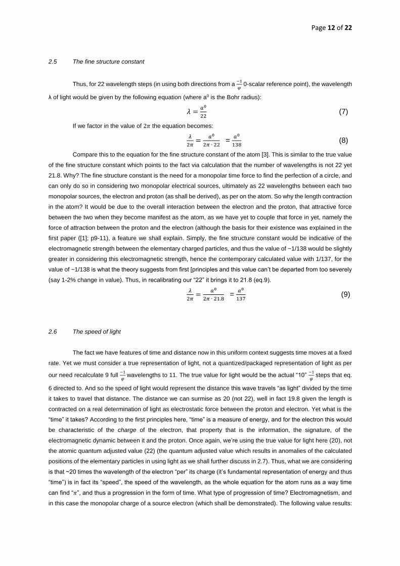
2.5 The fine structure constant

Thus, for 22 wavelength steps (in using both directions from a −1

𝜑 0-scalar reference point), the wavelength

λ of light would be given by the following equation (where a0 is the Bohr radius):

𝜆 =𝑎0

22 (7)

If we factor in the value of 2𝜋 the equation becomes:

𝜆

2𝜋=

𝑎0

2𝜋 ∙ 22 =

𝑎0

138 (8)

Compare this to the equation for the fine structure constant of the atom [3]. This is similar to the true value

of the fine structure constant which points to the fact via calculation that the number of wavelengths is not 22 yet

21.8. Why? The fine structure constant is the need for a monopolar time force to find the perfection of a circle, and

can only do so in considering two monopolar electrical sources, ultimately as 22 wavelengths between each two

monopolar sources, the electron and proton (as shall be derived), as per on the atom. So why the length contraction

in the atom? It would be due to the overall interaction between the electron and the proton, that attractive force

between the two when they become manifest as the atom, as we have yet to couple that force in yet, namely the

force of attraction between the proton and the electron (although the basis for their existence was explained in the

first paper ([1]; p9-11), a feature we shall explain. Simply, the fine structure constant would be indicative of the

electromagnetic strength between the elementary charged particles, and thus the value of ~1/138 would be slightly

greater in considering this electromagnetic strength, hence the contemporary calculated value with 1/137, for the

value of ~1/138 is what the theory suggests from first [principles and this value can’t be departed from too severely

(say 1-2% change in value). Thus, in recalibrating our “22” it brings it to 21.8 (eq.9).

𝜆

2𝜋=

𝑎0

2𝜋 ∙ 21.8 =

𝑎0

137 (9)

2.6 The speed of light

The fact we have features of time and distance now in this uniform context suggests time moves at a fixed

rate. Yet we must consider a true representation of light, not a quantized/packaged representation of light as per

our need recalculate 9 full −1

𝜑 wavelengths to 11. The true value for light would be the actual “10”

−1

𝜑 steps that eq.

6 directed to. And so the speed of light would represent the distance this wave travels “as light” divided by the time

it takes to travel that distance. The distance we can surmise as 20 (not 22), well in fact 19.8 given the length is

contracted on a real determination of light as electrostatic force between the proton and electron. Yet what is the

“time” it takes? According to the first principles here, “time” is a measure of energy, and for the electron this would

be characteristic of the charge of the electron, that property that is the information, the signature, of the

electromagnetic dynamic between it and the proton. Once again, we’re using the true value for light here (20), not

the atomic quantum adjusted value (22) (the quantum adjusted value which results in anomalies of the calculated

positions of the elementary particles in using light as we shall further discuss in 2.7). Thus, what we are considering

is that ~20 times the wavelength of the electron “per” its charge (it’s fundamental representation of energy and thus

“time”) is in fact its “speed”, the speed of the wavelength, as the whole equation for the atom runs as a way time

can find “𝜋”, and thus a progression in the form of time. What type of progression of time? Electromagnetism, and

in this case the monopolar charge of a source electron (which shall be demonstrated). The following value results:

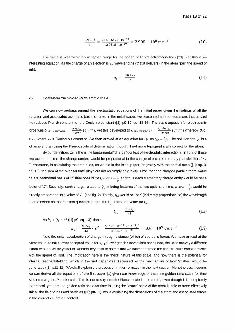
Page 13 of 22

19.8 ∙ 𝜆

𝑒𝑐=

19.8 ∙ 2.426 ∙ 10−12

1.60218 ∙ 10−19 = 2.998 ∙ 108 𝑚𝑠−1 (10)

The value is well within an accepted range for the speed of light/electromagnetism [21]. Yet this is an

interesting equation, as the charge of an electron is 20 wavelengths (that it delivers) in the atom “per” the speed of

light:

𝑒𝑐 = 19.8 ∙ 𝜆

𝑐 (11)

2.7 Confirming the Golden Ratio atomic scale

We can now perhaps amend the electrostatic equations of the initial paper given the findings of all the

equation and associated axiomatic basis for time. In the initial paper, we presented a set of equations that utilized

the reduced Planck constant for the Coulomb constant ([1]; p9-10, eq. 13-16). The basic equation for electrostatic

force was 𝑄𝐴𝐵<𝑁𝐸𝑊𝑇𝑂𝑁𝑆> =𝑄𝐶𝑄𝐴𝑄𝐵

𝑡𝐴𝐵𝑡𝐵𝐴 (𝐶3𝑡−2), yet this developed to 𝑄𝐴𝐵<𝑁𝐸𝑊𝑇𝑂𝑁𝑆> =

𝑄𝐶𝑐2𝑄𝐴𝑄𝐵

𝑑𝐴𝐵𝑑𝐵𝐴 (𝐶3𝑡−2) whereby 𝑄𝐶c2

= ke, where ke is Coulomb’s constant. We then arrived at an equation for QC as 𝑄𝐶 =𝛼ђ

𝑐𝑒2. The solution for QC is a

lot simpler than using the Planck scale of determination though, if not more topographically correct for the atom.

By our definition, QC is the is the fundamental “charge” context of electrostatic interactions. In light of these

two axioms of time, the charge context would be proportional to the charge of each elementary particle, thus 2𝑒𝑐.

Furthermore, in calculating the time axes, as we did in the initial paper for gravity with the spatial axes ([1]; pg. 9,

eq. 12), the idea of the axes for time plays out not as simply as gravity. First, for each charged particle there would

be a fundamental basis of “2” time possibilities, 𝜑 𝑎𝑛𝑑 −1

𝜑, and thus each elementary charge entity would be per a

factor of “2”. Secondly, each charge related to 𝑄𝐶 in being features of the two options of time, 𝜑 𝑎𝑛𝑑 −1

𝜑, would be

directly proportional to a value of √3 (see fig. 2). Thirdly, 𝑄𝐶 would be “per” (indirectly proportional to) the wavelength

of an electron as that minimal quantum length, thus 1

𝜆. Thus, the value for 𝑄𝐶:

𝑄𝐶 = 3 ∙2𝑒𝑐

4𝜆 (12)

As 𝑘𝑒 = 𝑄𝐶 ∙ 𝑐2 ([1] p9, eq. 13), then;

𝑘𝑒 = 3 ∙2𝑒𝑐

4𝜆 ∙ 𝑐2 =

6 ∙ 1.6 ∙ 10−19 ∙ (3 ∙108)2

4 ∙2.426 ∙10−12 = 8.9 ∙ 109 𝐶𝑚𝑠−2 (13)

Note the units, acceleration of charge through distance (which of course is force). We have arrived at the

same value as the current accepted value for 𝑘𝑒 yet owing to the new axiom base used, the units convey a different

axiom relation, as they should. Another key point to note is that we have confirmed the fine structure constant scale

with the speed of light. The implication here is the “held” nature of this scale, and how there is the potential for

internal feedback/folding, which in the first paper was discussed as the mechanism of how “matter” would be

generated ([1]; p11-12). We shall explain the process of matter-formation in the next section. Nonetheless, it seems

we can derive all the equations of the first paper [1] given our knowledge of this new golden ratio scale for time

without using the Planck scale. This is not to say that the Planck scale is not useful, even though it is completely

theoretical, yet here the golden ratio scale for time in using the “exact” scale of the atom is able to more effectively

link all the field forces and particles ([1]; p8-12), while explaining the dimensions of the atom and associated forces

in the correct calibrated context.

Page 14 of 22

2.8 Subatomic electrodynamics and Gravity’s emergence thereof

Let’s investigate the internal feedback/folding the following equation 14 points to by applying eq.11 to eq.

13:

𝑘𝑒 = 3 ∙2 ∙ 20 ∙ 𝑐

4 = 30𝑐 (14)

This result is telling; it states that the electromagnetic coupling force context is a value of 30𝑐. Note, as

this would be a “pre-event” prior electromagnetic interaction, as a building up process to the formation of the

elementary particles, the factor used would be 20, as it’s “after” the coupling constant is used that the

electromagnetic interaction is reduced from the theorised “20” factor down to “19.8” (fig. 16). Nonetheless, the

result states that given the speed of light is a feature of the radius of the atom per “charge” 𝑐 = 19.8 ∙ 𝜆

𝑒𝑐, then we

have a situation of “30” times this radius value in effect. Given the radius is fixed though, we could only have a

“running to and from” in effect for light, from the electron location to the proton, of light, of the time-wave (fig 14.):

30c Subatomic/elementary functionalities

electron proton

Figure 14; 15 “c” directions from the electron to the proton, and 15 “c” directions from

the proton to the electron, each loop meriting a new unique status/orientation of the

electron and proton.

How this “running and returning” of light would manifest between the electron and proton, between these

elementary charged particles (their status as “particles” to be explained later in this section), would define with each

“running and returning” a unique status, a unique orientation, or a unique sub-structure, any combination thereof,

of these elementary charged particles. Given the nature of the electron, it would be reasonable to suggest that it

would exist more than likely than not in various locations around the proton according to its need to circumscribe a

circle (condition for −1

𝜑, eq. 3), like in a “cloud” of 15 various positions, whereas the proton (and neutron, as we

shall soon explain) would although be relatively fixed in the atom, would have substructures meriting the 15 different

unique identifiers they would need to uphold (whatever they may be while depending on the two as-yet announced

features of the Uncertainty Principle and Quantum Entanglement effective a particles status, as per the explanation

in section 2.9) (fig.15):

Page 15 of 22

proton electron “cloud”

Figure 15; 15 “c” orientations for the electron to the proton, and 15 “c” internal

sub-structure ingredients for the proton, once again each of the 30 “c” loops

meriting a new unique status/orientation of the electron and proton.

It should be noted that each of these “c” loops would form the electrodynamic binding substructure of the

electrodynamic force between charged elementary particles. This would be a feature “primarily” of the electrical

component given its monopolar “𝜋” status. Note that these 30c loops represent two key electrodynamic reflection

points, opposite to each other in their effect, yet attractive to each other nonetheless in keeping the fine structure

pegged at the value it must be. Thus, on a fundamental level we would have a virtually massless (as electrical

energy) charge as the electron and its opposite as an oppositely charged mass (logically) as the proton. We know

we have the magnetic dipole moment, thus we would have its opposite as mass without charge, the neutron. All

these features are a fundamental result of the need to uphold polar/opposite reflection points knitting together 30c

substructure features relevant to their own status.

Can we dive deeper though into the relationship between charge and mass?

What of the virtual “magnetic (𝜑)” component from the 0-scalar “electrical (−1

𝜑) standpoint/basis”? If we

factored in the “4.58” value of the virtual magnetic (−1

𝜑 𝑓𝑜𝑟 𝑡𝑏

2) component (eq. 5), the value of “𝑘𝑒” becomes ~137.

But this is no longer 𝑘𝑒, yet a new entity, for we are not considering the factor of “𝜋” any more, but the magnetic

feature. Thus, this new factor would apply not to the electron and proton as subatomic charged constructs (already

satisfying 𝜋), but to the neutron (as the polar associate to magnetism, as explained) primarily. Why? The “𝑐” factor

is related “by-definition” to the electrical component, the “𝜋” feature (eq. 3, eq. 6). So, this new “factor” of 137 raises

an interesting situation, for it is the value of 1

⍺. Note this value is a “supplementary” feature of the 𝑘𝑒 = 30𝑐 subatomic

feature occurring, and thus would represent an “overarching” process upon this 30𝑐 feature/phenomena of the

atomic electrodynamics, and thus most basically as a simple folding of light as 𝑐2 and not 2𝑐 (as 2𝑐 would be a

feature embedded in the 30𝑐 manifold, as we shall now explain why).

According to the initial paper [1], this would represent a “mass” effect that is 137 times stronger than the

underlying electrodynamic subatomic process occurring. Consider eq. 18 and eq.19 of the initial paper [1], 𝑀(𝑝+𝑒)

𝛼 ≅

128 𝐺𝑒𝑉𝑐−2, 𝑚𝑎𝑠𝑠(𝑎𝑡𝑜𝑚𝑖𝑐)

𝐻0(𝐻𝑖𝑔𝑔𝑠 𝑝𝑎𝑟𝑡𝑖𝑐𝑙𝑒 𝑚𝑎𝑠𝑠)≅ 𝛼. There, the proposal was that the Higgs mass (there, taken as ≅

128 𝐺𝑒𝑉𝑐−2) is 137 times stronger than the atomic mass. In other words, the Higgs mass could in fact be the 30-

subatomic feature of the magnetic component of the atom that gives the atom its “mass” properties, the “atomic”

Page 16 of 22

mass itself being measured as a component primarily of the electrodynamic magnetic scale given the Higgs particle

mass (measured as 𝑒𝑛𝑒𝑟𝑔𝑦

𝑐2) is 137 greater than that of the mass of the proton, clearly pointing to the amount of

energy in the substructure of the atom undertaking this manifestation and why. Experimental results though pointed

the Higgs mass to be 125 𝐺𝑒𝑉𝑐−2 and not 128 𝐺𝑒𝑉𝑐−2. Nonetheless, we could confirm through these results given

the use of this equation in preliminary research the following (eq. 15):

𝑒𝑝 = 𝑚𝑝𝑐2 (15)

Once again, why is the “energy” of mass beyond the elementary 30c level, and more specifically,

proportional to mass and 𝑐2? Because all there would be “beyond” the 30c manifold is a “c” factor that can only be

“squared” as a “future” event beyond the primary 30c “now” event (fig. 16). This therefore confirms the initial paper’s

provisional proposal of “mass” being a 𝑡𝐴 entity, a squaring of 𝑡𝐵, noting also that the provisional proposal in that

paper was placing energy on “𝑡𝐵” (see requirement of [1]; eq.3, p4).

atomic functionalities Electron shell tA (tB2) modelling atomic functionalities

Contraction of scale from 22 to 21.8 via e-p interaction

electron Emergent feature of c2 (dual light) with mass proton/neutron

energy emergence as “mass” and 𝑐2 (𝑡𝐴2)

(magnetic feature)

elementary elementary

functionalities functionalities

Figure 16; “beyond” the 30c manifold is a “c” factor that can only be “squared” as a “future” (ta2) event

beyond the primary 30c “now” event. Note also the contraction of the atomic scale from 22 to 21.8 owing

to the emergent force between the electron and the proton, and subsequent electron shell modelling.

It’s also important to note the contraction of the atomic scale from 22 to 21.8 by the emergent force

between the proton and the electron. Furthermore, electrons would behave in their cloud orientation in this new

emergent platform according to what was proposed in the initial paper regarding the Rydberg equation ([1]; p12-

15). Here, we are confirming the tA status of this emergent level which allowed us to derive the electron shells in

the initial paper ([1]; p12-15). Note that we are also incorporating in the adjusted value of the atomic length from

19.8 to 21.8, and thus entertaining these “quantum additions” regarding the electron shell modelling as proposed

in the initial paper ([1]; p12-15). In doing so, if we consider the principle of the subatomic functionalities (equation

14) as a “carry through effect” from the subatomic/elementary level with this new emergent level of energy shells,

the following equation results:

𝑘𝑒 = 3 ∙2 ∙ 21.8 ∙ 𝑐

4 = 32.7𝑐 (16)

Page 17 of 22

Basically, there would be on this electron shell emergent level only a maximum of “32” full orientations

for each electron shell level if indeed the proton and neutron must remain fixed as mass entities undertaking a

strong-force of association ([1]; p12). The Rydberg Formula presents that the following series of electrons in shells

is allowable: 2, 8, 18, 32, 50, 72 [19]. Here though we are stating that it is not possible for an energy shell to go

beyond 32 electrons. And this is indeed correct with the Periodic Table [21] where the elements are unable to

reach the “50” occupancy level for an energy shell. It seems therefore we have capped the development of an

atom (confirmed with what is found in nature) by the application of the golden ratio as an algorithm for time.

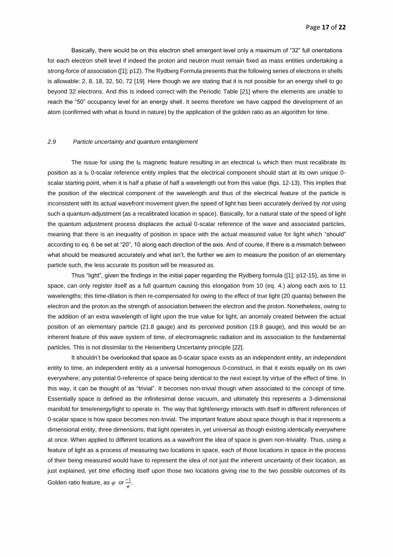
2.9 Particle uncertainty and quantum entanglement

The issue for using the tB magnetic feature resulting in an electrical tA which then must recalibrate its

position as a tB 0-scalar reference entity implies that the electrical component should start at its own unique 0-

scalar starting point, when it is half a phase of half a wavelength out from this value (figs. 12-13). This implies that

the position of the electrical component of the wavelength and thus of the electrical feature of the particle is

inconsistent with its actual wavefront movement given the speed of light has been accurately derived by not using

such a quantum-adjustment (as a recalibrated location in space). Basically, for a natural state of the speed of light

the quantum adjustment process displaces the actual 0-scalar reference of the wave and associated particles,

meaning that there is an inequality of position in space with the actual measured value for light which “should”

according to eq. 6 be set at “20”, 10 along each direction of the axis. And of course, if there is a mismatch between

what should be measured accurately and what isn’t, the further we aim to measure the position of an elementary

particle such, the less accurate its position will be measured as.

Thus “light”, given the findings in the initial paper regarding the Rydberg formula ([1]; p12-15), as time in

space, can only register itself as a full quantum causing this elongation from 10 (eq. 4.) along each axis to 11

wavelengths; this time-dilation is then re-compensated for owing to the effect of true light (20 quanta) between the

electron and the proton as the strength of association between the electron and the proton. Nonetheless, owing to

the addition of an extra wavelength of light upon the true value for light, an anomaly created between the actual

position of an elementary particle (21.8 gauge) and its perceived position (19.8 gauge), and this would be an

inherent feature of this wave system of time, of electromagnetic radiation and its association to the fundamental

particles. This is not dissimilar to the Heisenberg Uncertainty principle [22].

It shouldn’t be overlooked that space as 0-scalar space exists as an independent entity, an independent

entity to time, an independent entity as a universal homogenous 0-construct, in that it exists equally on its own

everywhere; any potential 0-reference of space being identical to the next except by virtue of the effect of time. In

this way, it can be thought of as “trivial”. It becomes non-trivial though when associated to the concept of time.

Essentially space is defined as the infinitesimal dense vacuum, and ultimately this represents a 3-dimensional

manifold for time/energy/light to operate in. The way that light/energy interacts with itself in different references of

0-scalar space is how space becomes non-trivial. The important feature about space though is that it represents a

dimensional entity, three dimensions, that light operates in, yet universal as though existing identically everywhere

at once. When applied to different locations as a wavefront the idea of space is given non-triviality. Thus, using a

feature of light as a process of measuring two locations in space, each of those locations in space in the process

of their being measured would have to represent the idea of not just the inherent uncertainty of their location, as

just explained, yet time effecting itself upon those two locations giving rise to the two possible outcomes of its

Golden ratio feature, as 𝜑or −1

𝜑.

Page 18 of 22

What exactly is the idea of quantum entanglement with particles? It would be related to the state of any

particle in relation to another particle as per a feature aside from the electromagnetic signal that relates directly

between them, and thus an apparent ‘immediate” effect related to the spatial status/orientation of the particles in

entanglement divined by the quality of the universally apparent 0-scalar spatial platform which itself doesn’t

represent as an a-priori timed speed limit (only light as time does). On the atomic scale, as when considering an

atom, the idea of quantum entanglement represents the two states that can be activated as a type of “vibration/spin”

for each particle along the sinusoidal train in relation to particles (as proposed in the initial paper [1]), as it only can,

for the two results are embedded already “in” the sinusoidal construct. The idea of the measurement itself of two

bodies using time/light creates an arena of light-measurement and thus a quantum association that places at a

minimum two bodies as either states of the golden ratio, owing to that golden ratio nature of light and thus arbitrary

measurement between any two particles through space. Essentially, it is an effect of the process of measurement,

and could be considered as an impossible causality of time given information cannot be transferred faster than the

speed of light, yet effectively would be a feature of space keeping two events in space at the one time linked in a

quantum-entangled manner. Quantum entanglement thus would represent a feature of space which would appear

to defy the idea of the speed of light by creating an immediate relativity for each strand (binary feature, 𝜑or −1

𝜑) of

golden ratio time. Once again, why? Because of how space is being defined, 0-scalar, universal, no limits. “Time”

as electromagnetic radiation is the limiting feature, and thus considering any two hypothetical points in 0-scalar

space would consider time to have arrived at any two points equally creating the idea of 𝜑and −1

𝜑 entanglement.

The amount of entanglement would depend therefore on the amount of considered observed reference

(measurement) between two independent (yet paradoxically not owing to time) spatial references. Owing to the

universal state of space and time, space being bathed in time as electromagnetic radiation, light, then everything

would be in a type of quantum entanglement with everything around it, the degree depending on all the factors the

that make the state of the system what it is.

2.10 Extra-atomic topology

In the initial paper, the idea of “fractal topology” ([1]; p15-16) was presented regarding the way space and

time would organise with all the relevant emergent forces between the considered theoretical golden ratio particles

in 0-scalar space (which of course would be infinite). First though, let’s consider what happens beyond the

subatomic scale, beyond the 30 unique underlying signatures of the elementary particles, while bearing in mind we

would need to factor in both the particle uncertainty and quantum entanglement principles, making the subatomic

realm a very difficult field of analysis. Fundamentally, the effect of light/time beyond the subatomic realm is defined

by the energy-shell play, as discussed in the initial paper ([1]: p13-15). The idea of particle uncertainty and quantum

entanglement would still apply to atoms and molecules, not just as elementary particle spin/orientation seen within

the atom, yet choice of motion in each now event (tN = 1), which as a choice between two unit values of time as a

location in space, two potential particles in a “now” event quantum entanglement, would result in a √2 value for

that resulting emergent (from the subatomic time-axes) now-time (fig. 17), suggesting that the random position of

a particles after factoring all previous atomic requirements is dependent on a √2 value for a resultant “now” time tN

in regard to space. This is not dissimilar to the equation Einstein reached for Brownian motion [23] (𝑥2

2𝑡= 𝐷, 𝑡ℎ𝑢𝑠 𝑥 =

𝐷√2𝑡). Here (fig. 17) the location (𝑥) of a particle in space would be proportional to √2 as a value of tN:

Page 19 of 22

1 √

1

Figure 17; two axes of time tN, 1 and 1, which then result in the

value of √2in a squared relationship as a resultant value of tN.

Beyond this, as highlighted in the initial paper [1], the idea of time going from time-before tB to time-after

as tB2 indicates a forever expanding spatial matrix, which is in fact a feature of light, an “effect”, or to be more

precise, an “illusion” set upon space by light ([1]; p16-17) [24]. Once again, this theorized perceived expansion of

the Universe (owing to the golden ratio time algorithm) would as “light” represent the key feature of light on the

atomic level as the “inverse” of the frequency of a Compton wavelength (𝜆𝑒

𝑐 ~ 8.1 ∙ 10-19 s), yet “squared” (tB2), and

thus a value of roughly 10-36 s (exactly 6.7 ∙ 10-37 s). The idea here is that with each oscillation of energy of the

electron, there would be a squaring effect in play as a time-front into the future, which of course would suggest

such a rate of expansion of space (as measured through the electromagnetic spectrum). Yet this is a theoretical

value, as a tA entity. Thus the “red-shift” [25] effect would be a key-part of that tB2 process; as light (as defined as

time) appears to be expanding, it would have the “same” effect on space by our definitions here, and thus make us

consider “space” is expanding ultimately in the farthest reaches of observation and calculation at an accelerating

rate.

The proposed fractal topology of space and time beyond atoms as discussed in the initial paper ([1]; p15-

16) would inherently require the balancing of all atoms, those atoms through their valence (electron shell)

association into molecules, and so on, with the feature of tB2 incurred, across an infinite 0-scalar manifold in

presuming 0-scalar space could exist anywhere. In not calibrating tB2 through vast distances, the effect “would” be

like a big-bang of an atomic level of time, as regarding the energy of the golden ratio time determination, that has

happened in every point in space at the same time. Confirmation of this possibility of atomic fractal displacement

in our analysis of perceived neutron stars is that neutron stars as observed to our calculations do indeed have a

distinct “magnetic” component [26], and thus as though a feature fractally sprung from the atomic to the universal,

clearly suggesting a fractal connecting pattern at play. Yet that phenomena appears not fractal to every reference.

Basically, the fractal topology of each reference in 0-scalar space would need to interact with each other reference,

and thus only logically there could be no “one” beginning reference given the actual state of a standard atom. So,

where would an ultimate reference come from, given that such is a clear drive of scientific thought for our need to

find that event-archaic?

2.11 Consciousness

Given the proposals of sections 2.7-10, there would appear to be an inherent mismatch between

“observation” and “calculation” regarding any elementary particle, together with an inherent universal entanglement

between all particles care of a feature of observation. This mismatch and entanglement could be considered as

Page 20 of 22

giving rise to a third concept especially considering our drive to find an ultimate event-archaic. So here it is proposed

such to be the very idea of consciousness [27] itself, a talent that allows us to think beyond what can’t be, and as

implicated here a type of dual nature of consciousness forever trying to resolve the mismatch between what is

observed and what is calculated, while entertaining a common 𝜑or −1

𝜑 nature for each construct set of observed

entities, as though in an immediate entangled sense, pure calculation being relative blindness, and pure

observation being relative miscalculation, all upon a universal 0-scalar “immediate” platform of consideration while

light as time plays back and forth in that seemingly supernatural immediacy. The proposition here is that

consciousness could well be described as being that “thing” that appears to be a supernatural feature of reality, a

feature in making observation and calculation as one. This will be the topic of a subsequent paper given the strictly

scientific nature of the paper presented here.

3 Conclusion:

This paper confirms that the most basic feature of space and time, the most fundamental drive, the golden

ratio for time in a 0-scalar universal space manifold, is the ultimate structure of the elementary particles, as per the

results found:

- An explanation for the monopolar nature of electricity, and dual-polar nature of magnetism.

- The fine structure constant derived from a golden ratio utility of time as applied to space.

- The speed of light derived from an electron wavelength, electron charge, and the fine structure

constant.

- An explanation to the space and time granularity of the subatomic level.

- An explanation for the uncertainty principle, namely the difference between what light measures and

where an elementary particle would be placed.

- An explanation for quantum entanglement for elementary particles, intricately associated to the

uncertainty principle.

- Confirmation for Brownian motion.

- An explanation as to why we would consider the event of a big bang and at what time-scale.

- An introduction to the idea of consciousness from the need of space and time to find synthesis

between observation and calculation anomalies alluding to the possibility of a fundamental ultimate

“eternal-archaic-event” of consciousness.

These results have been achieved in this paper “upon” the already derived features of the initial paper

“Gravity’s Emergence from Electrodynamics” [1]. Subsequently, this paper clearly is suggesting the Planck scale

of determination has well over-shot the mark, has dived too deeply into the theoretical granularity of space and

time, and thus is purely theoretical with no actual space and time granularity promise. This would therefore dismiss

the idea of a string theory on the Planck scale as a way of approaching a theory of everything. Moreover, regarding

cosmology, if light gives the effect of an accelerating expanding spatial matrix, and this is an illusion of time, was

there a big bang? As per the initial paper [1], the tB of an electron wavelength is 𝜆𝑒

𝑐 ~ 8.1 ∙ 10-19 seconds, and on an

expanded spatial scale it’s tA and thus 6.7 ∙ 10-37 seconds. Without understanding tA, we would consider time in the

vast expanse of space to be a singular concept of time. According to our first principles here for the Golden Ratio,

anything that represents a vast distance ahead represents the idea of tA, it has to, so measuring the rate of

expansion of the universe based on time must take into consideration the effect of tA. Is therefore the multiverse

theory a relevant possibility as an offshoot of an expanding Universe?

Page 21 of 22

The basic feature of this paper is how simple space and time can be understood when taking upon the

right tools of measurement as an a-priori. There are countless examples in history where using the right tools to

start with can alleviate massive amounts of inefficiency of observation and thought. For instance, using the wind in

a sail is far more effective than paddling, just like a jet engine is far more useful than a standard prop-engine. Why

has the golden ratio been overlooked for so long? Simply because we’ve all been victim to the belief that “time” is

what a clock measures. It’s like saying “space” is what a ruler measures. Both are fails, because a clock and a ruler

become fundamental entities in that process of determination, which is absurd, as both are in fact “results” of our

observation and calculation efforts of space and time, not fundamental entities themselves that explain the basis

of time and space as fundamental entities separate to what results thereof. Let’s therefore recap what was

presented in the first paper.

The idea of tA = tB2, and tB + 1 = tA is the edge. From a value in the past as tB the future arrives as tB2

provided within that step of time a “1” value is added. It’s mathematics with conditions, two conditions, as

pronounced. As that mathematics shows, there can be two values for tB, and thus two values of tA. Why? Why

those first principles for time? Given the one-directionality of time, and that’s the key, time as we know it can only

be what has happened in time added to a unitary value if indeed we are creating a unitary standard for time as “1”

for time “now”. The result of this is a squaring of “time past” given “time now” would need to still exist as a unitary

basic value. It’s as though time now as the addition of “1” to time before creates a spatial skewing of “time before”

as dual-time of “time past”, as tB2. Simply, adding “1” to a number creating a square of that value independently

when added to 1 suggests the idea of “1” as “time now”, while the other number as “time before” suggests an arrow

unlike the initial equation of “time before” plus 1, otherwise it would be a simple cycle of tB +1 = tB + 1. The only

result can be tA = tB2 given all we are allowed to use in not corrupting the singularity of “time now” is tB multiplied

by itself as the result for tA. Words can only convey as much as words can, but the results speak for themselves.

No one knew, has known, that tB + 1 = tA (tB2) is a golden ratio equation. So, it’s been overlooked. More

fundamentally, “now” appears to be the great divider as a value of “1”. And as the results show, the division

ultimately happens between observation and calculation, begging the question of an ultimate answer in the form

of consciousness, a unity of observation and calculation, a feature of our work forwards in time from times past,

the subject of a subsequent paper.

Conflicts of Interest

The author declares no conflicts of interest; this has been an entirely independent project.

References

1. Jarvis S. H. (2017), Gravity’s Emergence from Electrodynamics, http://viXra.org/abs/1704.0169?ref=9367626,

www.gravielectric.com.

2. Livio, Mario (2002). The Golden Ratio: The Story of Phi, The World's Most Astonishing Number. New York: Broadway

Books. ISBN 0-7679-0815-5.

3. Mohr, P. J.; Taylor, B. N.; Newell, D. B. (2015). "Fine structure constant", http://physics.nist.gov/cgi-bin/cuu/Value?alph,

CODATA Internationally recommended 2014 values of the fundamental physical constants. National Institute of

Standards and Technology,

4. International Bureau of Weights and Measures (2006), The International System of Units (SI) (PDF) (8th ed.), p. 112,

ISBN 92-822-2213-6Berggren, Lennart; Borwein, Jonathan; Borwein, Peter (1997).

5. Pi: a Source Book. Springer-Verlag. ISBN 978-0-387-20571-7.

6. "physics". Online Etymology Dictionary, http://www.etymonline.com/, Retrieved 2017-06-21.

Page 22 of 22

7. Garland, Jr., Theodore. "The Scientific Method as an Ongoing Process", http://physics.nist.gov/cgi-bin/cuu/Value?alph, U

C Riverside. Archived from the original on 23 Jun 2017.

8. "space - physics and metaphysics". https://www.britannica.com/science/space-physics-and-metaphysics, Encyclopædia

Britannica.

9. "Oxford Dictionaries:Time", https://en.oxforddictionaries.com/definition/time, Oxford University Press. 2011. Retrieved 23

JUne 2017. The indefinite continued progress of existence and events in the past, present, and future regarded as a

whole”

10. Hetherington, Norriss S. (2014). Encyclopedia of Cosmology (Routledge Revivals): Historical, Philosophical, and

Scientific Foundations of Modern Cosmology. Routledge. ISBN 978-1-317-67766-6.

11. Hawking, S. W.; Ellis, G. F. R. (1973). The Large-Scale Structure of Space-Time. Cambridge University Press. ISBN 0-

521-20016-4.

12. Kragh, Helge (1999). Cosmology and Controversy: The Historical Development of Two Theories of the Universe.

Princeton University Press. ISBN 0-691-02623-8.

13. David Deutsch (1997). "The Ends of the Universe". The Fabric of Reality: The Science of Parallel Universes—and Its

Implications. London: Penguin Press. ISBN 0-7139-9061-9.

14. J. A. McGovern,"2.5 Entropy". Archived from the original on 2012-09-23. Retrieved 2017-06-22.

15. Anderson, P.W. (1972). "More is Different" (PDF). Science. 177 (4047): 393–396. Bibcode:1972Sci...177..393A.

16. Eliel, Ernest Ludwig; Wilen, Samuel H. & Mander, Lewis N. (1994). "Chirality in Molecules Devoid of Chiral Centers

(Chapter 14)". Stereochemistry of Organic Compounds (1st ed.). New York, NY, USA: Wiley & Sons. ISBN 0471016705.

doi:10.1002/(SICI)1520-636X(1997)9:5/6<428::AID-CHIR5>3.0.CO;2-1.

17. quantum entanglement Schrödinger E (1935). "Discussion of probability relations between separated systems".

Mathematical Proceedings of the Cambridge Philosophical Society. 31 (4): 555–563. Bibcode:1935PCPS...31..555S.

doi:10.1017/S0305004100013554.

18. http://physics.nist.gov/cgi-bin/cuu/Value?plkmc2gev

19. Bohr, N. (1985). "Rydberg's discovery of the spectral laws". In Kalckar, J. Collected works. 10. Amsterdam: North-Holland

Publ. Cy. pp. 373–379.

20. Besant, W.H. (1907). "Chapter III. The Ellipse". Conic Sections. London: George Bell and Sons. p. 50.

21. Emsley, J. (2011). Nature's Building Blocks: An A-Z Guide to the Elements (New ed.). New York, NY: Oxford University

Press. ISBN 978-0-19-960563-7

22. Heisenberg, W. (1927), "Über den anschaulichen Inhalt der quantentheoretischen Kinematik und Mechanik", Zeitschrift

für Physik (in German), 43 (3–4): 172–198.

23. Einstein, Albert (1956) [Republication of the original 1926 translation]. "Investigations on the Theory of the Brownian

Movement" (PDF). Dover Publications. Retrieved 2017-06-22.

24. Tyson, Neil deGrasse and Donald Goldsmith (2004), Origins: Fourteen Billion Years of Cosmic Evolution, W. W. Norton &

Co., pp. 84–5.

25. Huggins, William (1868). "Further Observations on the Spectra of Some of the Stars and Nebulae, with an Attempt to

Determine Therefrom Whether These Bodies are Moving towards or from the Earth, Also Observations on the Spectra of

the Sun and of Comet II". Philosophical Transactions of the Royal Society of London. 158: 529–564.

Bibcode:1868RSPT..158..529H. doi:10.1098/rstl.1868.0022

26. Glendenning, Norman K. (2012). Compact Stars: Nuclear Physics, Particle Physics and General Relativity (illustrated

ed.). Springer Science & Business Media. p. 1. ISBN 978-1-4684-0491-3.

27. John Searle (2005). "Consciousness". In Honderich T. The Oxford companion to philosophy. Oxford University Press.

ISBN 978-0-19-926479-7.