Gold Deportment and Geometallurgical Recovery Model for ... · Gold-related veins include quartz-sulfide (A type) and sulfide ... techniques, a predictive geometallurgy model to estimate

Gold Deportment and Geometallurgical Recovery Model for the La Colosa, Porphyry

Gold Deposit, Colombia

Stacey Elizabeth Leichliter CODES/School of Earth Sciences

Submitted in fulfilment of the requirements for the

Masters of Science in Geology

University of Tasmania

May 2013

ii

Gold Deportment and Geometallurgical Recovery Model for the La Colosa, Porphyry

Gold Deposit, Colombia

Approved by Supervising

Committee:

Dr. Julie Hunt

Dr. Ron Berry

iii

Declaration

"This thesis contains no material which has been accepted for a degree or diploma by the

University or any other institution, except by way of background information and duly

acknowledged in the thesis, and to the best of the my knowledge and belief no material

previously published or written by another person except where due acknowledgement is

made in the text of the thesis, nor does the thesis contain any material that infringes

copyright.”

Signed:

_____________________ _______

Stacey Leichliter Date

Authority of Access

This thesis may be made available for loan. Copying and communication of any part of

this thesis is prohibited for two years from the date this statement was signed; after that

time, limited copying and communication is permitted in accordance with the Copyright

Act 1968.

Signed:

_____________________ _______


iv

Statement of Ethical Conduct

“The research associated with this thesis abides by the international and Australian codes on

human and animal experimentation, the guidelines by the Australian Government's Office of

the Gene Technology Regulator and the rulings of the Safety, Ethics and Institutional

Biosafety Committees of the University.”

Signed:

_____________________ _______


Statement regarding published work contained in thesis

“The publishers of the paper comprising Chapters 4 to 6 hold the copyright for that content,

and access to the material should be sought from the respective journals. The remaining non

published content of the thesis may be made available for loan and limited copying and

communication in accordance with the Copyright Act 1968.”

Signed:

_____________________ _______


v

Co-Authorship

The following people and institutions contributed to the publication of work undertaken as

part of this thesis:

Stacey Leichliter, CODES/University of Tasmania = Candidate

J. Hunt, CODES/University of Tasmania = Author 1

R. Berry, CODES/University of Tasmania = Author 2

L. Keeney, JK Tech = Author 3

P. Montoya, AngloGold Ashanti Colombia/JKMRC = Author 4

V. Chamberlain, AngloGold Ashanti Limited= Author 5

R. Jahoda, AngloGold Ashanti Colombia = Author 6

U. Drews, AngloGold Ashanti Colombia = Author 7

Author details and their roles:

“Development of a Predictive Geometallurgical Recovery Model for the La Colosa,

Porphyry Gold Deposit, Colombia”, 2011, GeoMet 2011 Proceedings, AusIMM:

Information located in Chapters 4 to 6 -

Candidate was the primary author and author 1 contributed to the idea, its

formalisation and development

Author 1, author 2, author 3, and author 4 assisted with refinement and

presentation

Author 5, author 6, and author 7 offered general geology, metallurgy, and

company assistance

Signed:

_____________________ _______


We the undersigned agree with the above stated “proportion of work undertaken” for each of

the above published (or submitted) peer-reviewed manuscripts contributing to this thesis:

Signed: _______________ _____ _________________ _____

Julie Hunt Date Bruce Gemmell Date

Supervisor Head of School

CODES/School of Earth Sciences CODES/School of Earth Sciences

University of Tasmania University of Tasmania

vi

ABSTRACT

The goal of this project was to develop a predictive geometallurgical recovery model for the

La Colosa porphyry gold deposit using the gold deportment, analytical data (multi-element

assays), mineralogy, and recovery data. The aim of geometallurgy is to reduce risk and

uncertainty by understanding the variability within the ore body, to increase the confidence in

forecasting and planning of production as well as optimizing recovery. Through different

levels of testwork, such as reference, support, and proxy, relationships and predictions are

made. Geometallurgy uses geology, statistics, and metallurgy to develop models that predict

the behaviour or variability in the ore body due to geological or mineralogical changes.

The La Colosa porphyry gold deposit is a world-class deposit located in the Central

Cordillera of Colombia. It is unusual because it is gold rich and has low amounts of copper

and trace molybdenum. The deposit consists of multiple intrusions of early, intermineral, and

late porphyritic phases of diorites, dacite, and quartz diorites that have intruded into the schist

and hornfels basement rock. The dominant alteration assemblage is potassic with weaker

amounts of potassic-calcic and sodic calcic alteration. Gold-related veins include quartz-

sulfide (A type) and sulfide (S and D type) veins. Geologic aspects of the deposit were used

to create a general geologic model for gold mineralisation at La Colosa that was used to help

create a recovery model.

The gold mineralisation at La Colosa occurs predominantly as native gold, gold tellurides,

and gold-silver tellurides, and in veins with a halo of disseminated (vein poor) gold

mineralisation. Grain size, association, and deportment of the gold at La Colosa were

vii

examined and the results used to understand the variability in the gold recoveries (cyanide

leach, gravity, and flotation). Recovery data was used with leaching as the primary process,

with tests such as shake leach and bottle roll analyses. Results of the geologic model,

detailed visual logging, gold recovery testwork, multi-element analyses, and mineralogy

testwork were used to build geometallurgical predictive models to estimate the gold recovery

using multivariate statistical techniques, such as correlation analysis, Mahalanobis Distance,

Principal Components Analysis (PCA), and multiple regressions. The steps used to develop

the geometallurgical model were the following:

1 Identify anomalies using Mahalanobis Distance.

2 Perform correlation analysis to identify similar characteristics.

3 Perform a Principal Components Analysis (PCA) to constrain variability and

develop discriminant diagrams for the data.

4 Define classes and perform linear and non-linear regressions to model the

desired parameter.

5 Create process performance domains of the data and wireframe to check.

6 Evaluate and re-iterate the model as newer data is gathered.

7 Apply to resource or geologic block model.

By using the recovery and gold mineralogy data along with the multivariate statistical

techniques, a predictive geometallurgy model to estimate gold recovery was constructed.

This model can be incorporated with the planning and resource models for the site to

efficiently extract and process the gold.

viii

ACKNOWLEDGEMENTS

I would like to thank Julie Hunt and Ron Berry for supervising my thesis work and providing

academic support throughout my graduate career. Their insight and knowledge have

improved my project and training greatly. I am grateful to Maya Kamenetsky for her

assistance with MLA instrumentation and data interpretation. I would like to thank Luke

Keeney at JKMRC for his assistance and knowledge in geometallurgical modelling

techniques. I also would like to thank the University of Tasmania’s ARC Centre of

Excellence in Ore Deposits (CODES) for providing me academic support. I am also grateful

for the University of Tasmania’s Central Science Laboratory and Karsten Goemann for use of

the MLA to analyse my samples. I would like to say thank you to the AMIRA P843A GeMiii

research team for their encouraging support and research into Geometallurgy.

I am extremely grateful to AngloGold Ashanti Limited, AngloGold Ashanti Colombia, and

Cripple Creek and Victor Gold Mine for giving me the opportunity to study this amazing

deposit. Without the financial support from AngloGold Ashanti Limited and Vaughan

Chamberlain, there would be no project for me to study. I owe them a huge thank you. I

would not be doing this without you. AngloGold Ashanti Colombia provided me with

excellent training from all their geologists. Thank you so much to Rudi Jahoda and his

geology team for teaching me everything about La Colosa. Special thanks go to Paula

Montoya and Andres Naranjo for taking time out of their days to help me with my many

questions. I am grateful to the entire La Colosa project team led by Jorge Tapia along with

their chief metallurgist, Udo Drews.

ix

Thank you to Cripple Creek and Victor Gold Mine for allowing me to fly around the world to

study. I appreciate the workload my coworkers had to undertake while I was away. Thanks

to Tim Brown in the Exploration Department for telling the company I was the best person

for the project. I owe you so much. Thank you to the AngloGold Ashanti again for this

opportunity.

I would finally like to thank my friends and family for their undying support and love through

this project. I really appreciate all you do for me, and I couldn’t have done this without you.

To my favourite editor, my Aunt Sue, I owe you a lot. Thank you to my family and friends

for giving me the strength to go out into the wide world and have great experiences.

This project was funded by AngloGold Ashanti as part of the AMIRA P843A

Geometallurgical Mapping and Mine Modelling (GeMIII

) project with the University of

Tasmania/CODES. AngloGold Ashanti Colombia provided the geological training, data, and

samples for the project. AngloGold Ashanti Limited provided the financial and educational

support for the project.

This research is part of a major collaborative geometallurgical project being undertaken at

CODES and SES (University of Tasmania), JKMRC, BRC and CMLR (Sustainable Minerals

Institute, University of Queensland) and Parker Centre CRC (CSIRO). The author

acknowledges financial support and permission to publish from industry sponsors of the

AMIRA International P843 and P843A GEMIII

projects – AngloGold Ashanti, Anglo

American, ALS, Barrick, BHP Billiton, Boliden, CAE Mining (Datamine), Codelco, Geotek,

Gold Fields, Golder Associates, ioGlobal, Metso Minerals, Minera San Cristobal, MMG,

Newcrest, Newmont, OZ Minerals, Penoles, Quantitative Geoscience, Rio Tinto, Teck, Vale

x

and Xstrata Copper (MIM). Financial support is also being provided by the Australian

Government through the CODES ARC Centre of Excellence in Ore Deposits and CRC ORE.

xi

TABLE OF CONTENTS

Declaration iii

Authority of Access iii

Statement of Ethical Conduct iv

Statement Regarding Published Work iv

Co-Authorship Statement v

Abstract vi

Acknowledgements viii

Table of Contents xi

List of Figures xvi

List of Tables xxi

Glossary xxiii

Abbreviations Contained in Thesis xxv

Chapter 1: Introduction 1

1.1 Study 1

1.1.1 Significance of Study 1

1.1.2 Methods 1

1.2 Background 4

1.2.1 Location 4

1.2.2 Exploration History 4

1.2.3 Ore Reserves 5

Chapter 2: Review of Regional Geology 6

2.1 Introduction 6

2.2 Regional Geology 7

2.3 Summary 10

Chapter 3: Review of La Colosa Geology 11

3.1 Introduction 11

3.2 Structural Setting of La Colosa 12

3.3 La Colosa Lithologies 15

xii

3.3.1 Hornfels/Schist 16

3.3.2 Early Diorites 17

3.3.3 Intermineral Diorites 22

3.3.4 Late Dacites and Quartz Diorites 23

3.4 La Colosa Alteration 25

3.4.1 Alteration Assemblages 25

3.4.2 Potassic 25

3.4.3 Potassic-Calcic 26

3.4.4 Calcic-Sodic 26

3.4.5 Quartz-Sericite 27

3.4.6 Intermediate Argillic 28

3.4.7 Propylitic 28

3.5 La Colosa Vein Types 28

3.5.1 Early Biotite 29

3.5.2 Magnetite 29

3.5.3 Quartz-Sulfide 30

3.5.4 Quartz-Sulfide with Suture 31

3.5.5 Sulfide 31

3.5.6 Sulfide-Quartz 32

3.5.7 Chlorite and Actinolite 33

3.6 Summary 33

Chapter 4: Review of Porphyry Copper-Gold and Porphyry Gold Deposits 35

4.1 Introduction 35

4.2 Terminology 35

4.3 Porphyry Copper-Gold Deposit Models 37

xiii

4.3.1 Deposit Model 37

4.3.2 Alteration and Veining 37

4.3.3 Mineralisation 39

4.4 Porphyry Copper-Gold Deposits 40

4.4.1 Bajo de la Alumbrera 40

4.4.2 Bingham Canyon 42

4.5 Porphyry Gold Deposit Models 44

4.5.1 Deposit Model 44

4.5.2 Alteration and Veining 45

4.5.3 Mineralisation 46

4.6 Porphyry Gold Deposits 47

4.6.1 Marte 47

4.6.2 Refugio District (Verde and Pancho) 49

4.7 Summary 51

Chapter 5: Gold Mineralisation 55

5.1 Introduction 55

5.2 Methods 55

5.2.1 Introduction 55

5.2.2 Sampling and Preparation 56

5.2.3 Analysis 58

5.2.3.1 Deposit Models 58

5.2.3.2 MLA Testwork 59

5.3 Gold Mineralogy 61


5.3.2 Types of Gold Mineralisation 61

xiv

5.3.3 Location of Gold Mineralogy 64

5.3.4 Native Gold Mineralisation 70

5.3.4.1 Grain Size 70

5.3.4.2 Mineral Associations 73

5.3.4.3 Locking 75

5.3.5 Gold Telluride Mineralisation 76



5.3.5.3 Locking 79

5.3.6 Gold-Silver Telluride Mineralisation 80



5.3.6.3 Locking 83

5.3.7 Summary 83

5.4 Vein Rich and Vein Poor Mineralisation 84


5.4.2 Methods 85

5.4.3 Vein Rich Mineralisation 86

5.4.4 Vein Poor Mineralisation 88

5.4.5 Summary 89

5.5 Summary of Gold Mineralisation 90

Chapter 6: Predictive Geometallurgical Gold Recovery Model 93

6.1 Introduction 93

6.2 Gold Recovery Processes 94

6.2.1 Gravity Concentration 94

xv

6.2.2 Flotation Concentration 95

6.2.3 Cyanide (NaCN) Leaching 96

6.3 Geometallurgical Gold Recovery Modelling 97

6.3.1 Geometallurgical Modelling 97

6.3.2 Methods for Gold Recovery Modelling 100

6.3.3 Model 1: To Estimate Gold Recovery as Measured

by Shake Leach Tests 101

6.3.4 Model 2: To Estimate Gold Recovery as Measured

by Bottle Roll Tests 115

6.3.4.1 Model 2 – Multi-Element 117

6.3.4.2 Model 2 – XMOD 124

6.3.4.3 Model 2 – Calculated Mineralogy 131

6.3.5 Results 136

6.3.6 Summary 142

Chapter 7: Geometallurgical Recovery Model and Conclusions 144

7.1 Geometallurgical Recovery Model 144

7.2 Conclusions 147

7.3 Further Work 149

References 151

Vitae 156

Appendix A: Shake Leach Assay Information 159

Appendix B: Bottle Roll Information 161

Appendix C: Laser Ablation Information 163

Appendix D: Detailed Geologic Logs (Digital) 165

Appendix E: Photographs (Digital) 166

Appendix F: MLA Data (Digital) 167

Appendix G: Recovery Data (Digital) 168

Appendix H: Mahalanobis Distance 169

Appendix I: Principal Components Analysis 173

Appendix J: Published Papers 176

xvi

LIST OF FIGURES

Figure 1: Apparatus for shake leach assay testwork. 3

Figure 2: Apparatus for bottle roll testwork. 3

Figure 3: Cordillera map of the Northern Andes of Colombia. 6

Figure 4: Geologic and structural map of the La Colosa region . 8

Figure 5: Map of the Middle Cauca Metallogenic Belt. 13

Figure 6: Map of the geology and structure of the La Colosa deposit. 14

Figure 7: Geologic map from AngloGold Ashanti Colombia. 16

Figure 8: Altered hornfels. 17

Figure 9: Early diorite E0 with potassic alteration. COL112_262-264. 18

Figure 10: Early diorite E1. COL108_242-246. 18

Figure 11: Early diorite intrusion breccia EBX1. 19


Figure 13: Early diorite intrusion breccia EBX2. 20


Figure 15: Early diorite EDM. COL112_564-566. 21

Figure 16: Intermineral diorite I1. COL101_274-276. 22

Figure 17: Intermineral diorite intrusion breccia IBX. 23

Figure 18: Intermineral diorite I2. 23

Figure 19: Weakly altered dacite. COL028_204-206. 24

Figure 20: Potassic alteration (strong) in EBX2. COL062_222-224. 26

Figure 21: Potassic-calcic alteration in EBX1. COL108_54-56. 26

Figure 22: Calcic-sodic alteration (strong) overprinting potassic alteration in EBX2. 27

Figure 23: Quartz-sericite alteration overprinting potassic. COL111_582-584. 27

xvii

Figure 24: Propylitic alteration (chlorite and epidote). COL101_252-254. 28

Figure 25: Early biotite veins in EBX1. COL069_332-334. 29

Figure 26: Magnetite vein with feldspar halo in EBX2. COL062_264-266. 30

Figure 27: Quartz-magnetite-sulfide vein in IBX. COL062_432-434. 30

Figure 28: Quartz-sulfide with central suture in EDM. COL099_198-200. 31

Figure 29: Sulfide vein in E0. COL112_300-302. 32

Figure 30: Sulfide-quartz vein with quartz-sericite alteration halo in EBX2. 32

Figure 31: Actinolite-sulfide vein with feldspar alteration halo. COL069_352-354. 33

Figure 32: Telescoped model of a typical porphyry copper-gold system. 38

Figure 33: Porphyry copper-gold alteration and mineralisation model. 38

Figure 34: Vein types observed in a porphyry copper-gold deposit. 39

Figure 35: Geologic map of the Bajo de la Alumbrera deposit. 40

Figure 36: Geologic and structural map of the Bingham Canyon deposit. 43

Figure 37: Model of a porphyry gold deposit. 46

Figure 38: Vein types observed in porphyry gold deposits. 47

Figure 39: Geologic map of the Marte deposit. 48

Figure 40: Geologic map of the Refugio district (Verde and Pancho). 49

Figure 41 a-c: Simplified cross sections of the lithologies at La Colosa. 66

Figure 42 a-c: Simplified cross sections of the major alteration assemblages. 66

Figure 43 a-c: Simplified cross sections showing the major vein types. 67

Figure 44 a-c: Simplified cross sections showing the telluride and sulfide zones. 67

Figure 45: Grain size distribution of native gold mineralisation. 71

Figure 46: Summary for the mineral associations in the native gold mineralisation. 73

Figure 47 a-f: Examples of the major gold mineral associations. 74

Figure 48: Grain size distribution of the gold tellurides. 77

xviii

Figure 49: Summary for the mineral associations for the gold telluride mineralisation. 78

Figure 50 a-d: Mineral associations for gold telluride grains analysed. 79

Figure 51: Grain size distribution of gold-silver tellurides in the samples. 81

Figure 52 a and b: Gold-silver telluride mineral associations. 82

Figure 53: Summary of mineral associations for gold-silver telluride mineralisation. 82

Figure 54: Grain size distribution for the vein rich and vein poor samples. 87

Figure 55: Mineral associations for the vein rich vs. vein poor samples. 88

Figure 56: Input parameters for Mahalanobis Distance Model 1. 102

Figure 57: Distribution curve of input data for Model 1. 103

Figure 58: Input parameters for Model 1 PCA. 104

Figure 59: Model 1 – PC1 vs. PC2. 105






Figure 65: Multivariate scatter plot of PC1 vs. PC3. 109

Figure 66: Scatter plots for clustering. 109

Figure 67: Discriminant diagram for Model 1. 110

Figure 68: Estimated shake leach wireframes. 112

Figure 69: Data from September 2011 drill hole database. 113

Figure 70: Classified data from September 2011 drill hole database. 114

Figure 71: Estimated shake leach recoveries wireframes. 114

Figure 72: Inputs for Mahalanobis Distance for Model 2. 116

Figure 73: Distribution curve for recovery data for Model 2. 116

xix

Figure 74: Input parameters for Model 2 – Multi-Element PCA. 118

Figure 75: Model 2 – Multi-Element PC1 vs. PC2. 119






Figure 81: Multivariate plot of PC1 vs. PC2. 122


Figure 83: Discriminant diagram for Model 2 – Multi-Element. 123

Figure 84: Model 2 – XMOD PC1 vs. PC2. 125






Figure 90: Multivariate scatter plot PC1 vs. PC2. 128


Figure 92: Discriminant diagram for Model 2 – XMOD. 130

Figure 93: Model 2 – Calc. min. PC1 vs. PC2. 132






xx

Figure 99: Multivariate scatter plot PC1 vs. PC3. 134


Figure 101: Discriminant diagram for Model 2 – Calc. min. 135

Figure 102: Calculated vs. Measured gold recoveries 137

Figure 103: Calculated vs Measured gold recovery divided by Au grade 137

Figure 104: Linear regression model 138

Figure 105: Calculated vs. Measured gold recovery Model 1 139

Figure 106: Calculated vs. Measured gold recovery Linear Model 139

Figure 107: Wireframes for estimated shake leach – linear model 140

Figure 108: Recovery wireframes for Model 2 – Multi-Element. 141

Figure 109: Discriminant diagram for Phase 2 samples. 145

Figure 110: Classified Phase 2 data. 146

Figure 111: Phase 2 wireframes for estimated shake leach recovery 147

xxi

LIST OF TABLES

Table 1: Summary table for the porphyry copper-gold and porphyry gold deposits. 53

Table 2: Summary table for Phase 1 samples analysed by the SPL_Lt method. 62

Table 3: Summary table of samples, number of grains located, and grain sizes (PSSA)

for samples analysed by SPL_Lt. 63

Table 4: Examples of gold grain fineness. 65

Table 5: XMOD results for the Phase 1 and Phase 2 samples. 68

Table 6: QXRD data of weakly altered and strongly altered samples and key minerals. 69

Table 7: Grain size distribution for native gold. 71

Table 8: Summary table for calculated grain sizes by PSSA from SPL_Lt. 72

Table 9: Gold grain size by PSSA of mineral associations. 73

Table 10: Summary table for the mineral associations for the native gold mineralisation. 75

Table 11: Average locking for gold, gold telluride, and gold-silver telluride. 76

Table 12: Grain size distribution of gold tellurides. 76

Table 13: Mineral associations for the gold telluride mineralisation by lithology. 79

Table 14: Grain size distribution of gold-silver tellurides. 80

Table 15: Summary table of the mineral associations for the gold-silver telluride

mineralisation. 83

Table 16: Summary table of vein rich and vein poor samples. 85

Table 17: Modal mineralogy of vein rich and vein poor samples. 86

Table 18: PSSA of the gold mineralisation in the vein rich samples. 87

Table 19: Minerals associated with gold mineralisation in the vein rich and

vein poor samples. 88

Table 20: PSSA of the gold mineralisation of the vein poor samples. 89

Table 21: Correlations for Model 1 PCA. 103

xxii

Table 22: Eigenvectors for Model 1 PCA. 105

Table 23: Table of regression equations used to estimate gold recovery in Model 1. 111

Table 24: Correlations for Model 2 – Multi-Element PCA. 117

Table 25: Eigenvectors for Model 2 – Multi-Element PCA. 118

Table 26: Regression equations used for Model 2 – Multi-Element. 123

Table 27: Model 2 – XMOD Correlations for PCA. 124

Table 28: Model 2 – XMOD Eigenvectors for PCA. 125

Table 29: Model 2 – XMOD regression equations. 130

Table 30: Model 2 – Calc. min. correlations for PCA. 131

Table 31: Model 2 – Calc. min. eigenvectors for PCA. 132

Table 32: Model 2 – Calc. min. regression equations. 136

xxiii

GLOSSARY

Correlation: degree of interrelation between variable in a manner not influenced by

measurement units (dimensionless measure of joint variation).

Cyanidation: method for extracting gold from host rock using a cyanide solution (sodium or

potassium) and oxygen that allows the gold to dissolve in solution.

Disseminated: scattered distribution of a mineral, generally fine-grained.

Extraction: separation of a substance from its matrix.

Fineness: purity of gold or the concentration of silver in the gold (Marsden and House,

2006).

Flotation: chemical mineral separation method where hydrophobic minerals (sulfides) are

separated by preferential floating on the surface.

Gangue: valueless rock.

Geometallurgy: the practice of combining geology and geostatistics with metallurgy to

create a spatially or geologically based predictive model for mineral processing

plants.

Grain: a particle or mineral with a diameter of less than a few millimetres.

Groundmass: material between the phenocrysts in a porphyritic rock.

Liberation: degree of freedom of being locked with a mineral.

Multivariate: analysis of multiple variables simultaneously.

Paragenesis: formation sequence of mineral assemblages, veins, and ore deposits.

Particle: separable or distinct unit in a rock. May contain multiple grains.

Phenocryst: a large conspicuous crystal of the earliest generation in a porphyritic rock.

Porphyritic: a rock texture where there’s a distinct difference in the size of the crystals, with

at least one group of crystals obviously larger than another group.

Recovery: the proportion of metal extracted to total metal present.

Sulfide: a mineral characterised by the combination of a metal with sulfur.

Univariate: analysis of a single variable.

http://en.wikipedia.org/wiki/Geology

http://en.wikipedia.org/wiki/Geostatistics

http://en.wikipedia.org/wiki/Metallurgy

http://en.wikipedia.org/wiki/Mineral_processing

xxiv

Variability: a measurement at various spatial locations exhibits values that differ spatially

Vein: mineral filling of a fault or fracture.

xxv

ABBREVIATIONS CONTAINED IN THESIS

BSE: Backscattered Electron

LA-ICP-MS: Laser Ablation –Coupled Plasma – Mass Spectrometry

MLA: Mineral Liberation Analyser

PCA: Principal Components Analysis

PSSA: Phase Specific Surface Area

QEM SCAN®: Quantitative Evaluation of Minerals by Scanning Electron

microscope

QXRD: Quantitative X-Ray Diffraction

SEM: Scanning Electron Microscope

SPL_Lt: Refinement of sparse phase search (MLA) for minerals of interest

XMOD: Point counting technique (MLA) for fast modal analysis

Stacey Leichliter

Page | 1

Chapter 1: Introduction

1.1 Study

1.1.1 Significance of Study

The La Colosa deposit is a large, gold porphyry system with sub-economic copper

grades and trace molybdenum values (Lodder et al., 2010). Gold-only deposits

represent a unique end member of the porphyry deposit model (Sillitoe, 2000). This

project analysed the gold mineralisation, mineralogy and alteration assemblages to

determine a general paragenesis for gold mineralogy of the deposit and a

geometallurgical recovery model. The gold mineralisation was analysed for its

associations, texture, grain size, and deportment. The gold mineralisation information

was used to help understand the variability in gold mineralogy and grades throughout

the deposit. The gold mineralisation details were also compared to the recovery tests

(e.g. bottle roll and shake leach) and to predict the variability in the recovery of the

system. Understanding the different types of mineralisation and deportment, a

comprehensive predictive model to estimate recovery was constructed. Information

from the geometallurgical recovery model can be incorporated into a block model for

mining purposes, in order that potential issues and anomalies with recovery can be

identified and investigated, so that gold extraction is optimised.

1.1.2 Methods

Gold characterisation at La Colosa was determined by selecting samples that lie

within the proposed production pit boundaries. The cut-off grade for mining was

determined to be approximately 0.3 g/t at the time of the project. All samples selected

were above this gold grade and were chosen from the diamond drill core supplied by

Stacey Leichliter

Page | 2

the site. The samples were crushed to -4.75 mm (coarse rejects from analytical

assays) and a representative sample split was mounted into 24mm diameter epoxy

resin mount for Scanning Election Microscopy (SEM). Each sample was analysed

using the Mineral Liberation Analyser (MLA) for the modal mineralogy (XMOD

method) and gold search (SPL_Lt method). Further information on the methodologies

for each analysis is found in the chapters associated with their analysis and in the

report by Gu, 2003 and on FEI’s website for the MLA (FEI, 2012).

The modal mineralogy (XMOD) data and Quantitative X-ray Diffraction (QXRD)

data were used to determine the alteration assemblage mineralogy associated with the

gold. The gold search method (SPL_Lt) was used to analyse the gold grains located

within each sample for their grain size and mineral associations. The gold

associations, deportment, grain size, and texture were determined along with

deleterious and trace mineral occurrences and associations by using the Automated

Optical Microscope and Mineral Liberation Analyser (MLA). The gold occurrence

(e.g. vein versus disseminated) and paragenesis was also determined. The samples

also underwent recovery testing for cyanide leachability (shake leach assay and bottle

roll testwork) which was compared with the gold mineralogy. This comparison

allowed for the estimation of the gold recovery due to the variability in the gold

mineralogy.

The shake leach assay is a quick, optimistic analysis to determine the amount of

cyanide extractable gold. Testwork involves a crushed or pulverised rock, 200 mesh

(74 µm), and sample placed into a vessel with a cyanide solution (NaCN) and placed

on an agitator (Eberbach shakers) for 1 hour (Figure 1). The solution is then analysed

Stacey Leichliter

Page | 3

for the concentration of gold extracted by the cyanide. More information on the shake

leach assay procedure is located in Appendix A.

Figure 1: Shake leach assay testwork setup. (http://www.opticsplanet.com/eberbach-heavy-duty-

shaker-two-speed-eberbach-6010.html)

The bottle roll test is a more conservative analysis for the cyanide extractable gold. It

uses a rotating platform to roll bottles containing crushed or pulverised samples, 200

mesh (74 µm), for a minimum of 12 hours up to 48 hours (Figure 2). It also gives the

acid consumption rate and shows the kinetics of the cyanide leach (SGS, 2012). More

information on the bottle roll testwork is found in Appendix B.

Figure 2: Bottle roll test analysis setup. (http://www.essa.com.au/EssaProductsDetail.)

Data was utilised, along with recovery test data, to construct predictive

geometallurgical recovery data. The recovery model was calculated using specific,

proven multivariate statistical analyses, such as correlation analysis, Mahalanobis

Distance, and Principal Components Analysis (PCA).

http://www.essa.com.au/EssaProductsDetail

Stacey Leichliter

Page | 4

The nomenclature for La Colosa describes the lithologies, alterations, and vein types.

The lithologies were named according to the field observations, rather than detailed

petrographic analysis. Lithologies described in this study are consistent with those

used on site. The alteration and vein terminology follow the nomenclature of typical

porphyry deposits (see Chapter 3.2).

1.2 Background

1.2.1 Location

The La Colosa gold porphyry is located in the Central Cordillera of the Northern

Andes in Colombia approximately 8 km northwest of Cajamarca and 30 km west of

Ibague in the department of Tolima. The deposit is hosted by a large (1,200 m long

and 400 m wide) cluster of porphyritic intrusions (Lodder et al., 2010).

1.2.2 Exploration History

The La Colosa porphyry gold deposit was a grassroots discovery in 2006 by

AngloGold Ashanti (AGA) (Lodder et al., 2010). The initial exploration started in

2004 with four geologists doing systematic fieldwork and sampling in the region. The

deposit was one of several targets identified by an extensive field campaign collecting

soil, rock chip, and stream samples. Detailed lithology and structural mapping are

still in progress. AngloGold Ashanti commenced a diamond drilling program in

2007, located in the northern and central part of the deposit. To date, the site has

completed approximately 120 diamond drill holes for over 34,000 m. The deposit is

owned by AngloGold Ashanti and is currently in its prefeasibility stages (Lodder et

al., 2010).

Stacey Leichliter

Page | 5

1.2.3 Ore Reserves

The La Colosa deposit has an inferred mineral resource of 392.11 Mt at a cut-off

grade of approximately 0.98 g/t (AngloGold Ashanti 2010 Mineral Resource and Ore

Reserve Report, 2010). The majority of gold is associated with what are referred to

on site as “early diorites”. Less gold is associated with the “intermineral diorites” and

“hornfels” (Lodder et al., 2010).

Stacey Leichliter

Page | 6

Chapter 2: Review of Regional Geology

2.1 Introduction

The La Colosa deposit lies on the eastern flank of the Central Cordillera and has a

complex geologic history (Figure 3). Previous work on the regional geology of the

area around La Colosa includes work by Goossens (1976); Sillitoe et al. (1982);

Lozano (1984); Pulido (1988); Nunez (2001); Sillitoe (2007); Gil-Rodriguez (2010);

and Lodder et al. (2010). These reports provide interpretations on the lithologic,

structural, and metallogenic controls and settings for the region and its deposits.

Other sources of reference material are confidential internal AngloGold Ashanti

reports.

Figure 3: Map showing the three cordilleras of the Northern Andes of Colombia. The Western

Cordillera is on the left, then the Central in the middle, followed by the Eastern Cordillera on the right

side. The La Colosa deposit is labelled with the red star. Original map provided by Sadalmelik, I.

(2007).

Stacey Leichliter

Page | 7

The types of porphyry systems reported in Colombia and the Northern Andes are

dependent on the type of underlying crust (i.e. continental or oceanic) and regional

structural controls. Plate tectonics and the formation of the Northern Andes played

important roles in the development of the region. The different porphyry deposits

found in Colombia include porphyry copper, porphyry copper-gold, porphyry copper-

molybdenum, and porphyry gold.

2.2 Regional Geology

La Colosa (8 Ma) is located in the Middle Cauca metallogenic belt of the Central

Cordillera (Sillitoe, 2007). The Central Cordillera has a complex geologic history.

The Cauca River Valley is the western boundary, and the Magdalena River Valley is

the eastern boundary of the cordillera. There are two major north-northeast fault

systems that bound the Colosa deposit on the west and east, the Romeral and

Palestina. To the east and south of the deposit is the Palestina fault, which originated

as a suture to the Cajamarca-Valdivia terrane in the early Paleozoic (Figure 4)

(Lodder et al., 2010). During the late Triassic-Jurassic, middle Cretaceous, late

Cretaceous-Paleocene, and Miocene, the Palestina fault was reactivated. The

reactivations appear to have aided in the emplacement of arc-related magmas, which

formed and developed the modern-day northern Andes volcanic arc (Lodder et al.,

2010). The Romeral fault is thought to be the suture between oceanic crust to the

west and continental crust to the east (Goossens, 1976).

Stacey Leichliter

Page | 8

Figure 4: Geologic and structural map of the La Colosa region. Map from Lodder et al. (2010)

modified from Cediel and Caceres (2000) and Nunez (2001).

The La Colosa deposit is located in the eastern part of the Cordillera which has

thicker (35 km - 45 km) continental crust, assumed to be the northwestern edge of the

Guyana Shield (Irving, 1971; Sillitoe et al., 1982). The basement rocks include pre-

Mesozoic low grade metamorphic rocks that are interpreted to have been sedimentary

shelf sequences to the east with increasing volcanic material to the west (Sillitoe et

al., 1982). Mesozoic stock and batholiths related to subduction intruded the basement

rocks (Taboada et al., 2000; Gil-Rodriguez, 2010).

Cordilleran-type orogenesis and regional metamorphism occurred in the sequence of

the South American plate during the early Paleozoic, and the terranes sutured along

the Palestina fault system (McCourt et al., 1984; Cediel et al., 2003; Kennan and

Pindell, 2009; Gil-Rodriguez, 2010). Intracontinental rifts, including the Bolivar

aulacogen (Late Paleozoic – Early Cretaceous) and Valle Alto rift (Early Cretaceous)

Stacey Leichliter

Page | 9

facilitated marine and continental sequences and intrusions. The period of extension

ended in the Early Cretaceous (125 Ma to 100 Ma), and then compression occurred

until recently (Aspden et al., 1987; Cediel and Caceres, 2000; Cediel et al., 2003; Gil-

Rodriguez, 2010).

The western part of the Central Cordillera is comprised of numerous accreted oceanic

terranes. The Farallon and South American plates shifted their direction and velocity

in the mid-Cretaceous new oceanic plates were formed from the oblique collisions,

subductions, and obductions, which also describe the northern Andean orogeny

(Pindell and Kennan, 2001, 2009; Cediel et al., 2003; Kennan and Pindell, 2009; Gil-

Rodriguez, 2010). Oceanic terranes have accreted along the Romeral-Cauca fault

zones since the mid-Cretaceous and have undergone periods of uplift, erosion, and

subduction-related magmatism along with part of the western part of the Central

Cordillera and Western Cordillera (Cediel et al., 2003; Gil-Rodriguez, 2010).

The presence of young stratovolcanoes along the crest of the Central Cordillera

suggests an eastward migration of the magmatic focus from the Miocene. The

Eastern Cordillera experienced a transpressive pop-up during the late Miocene-

Pliocene and has undergone extensive erosion. Present structural environment

includes reactivation of the Palestina and Romeral systems, which faulted and

disrupted the late Miocene intrusions and their associated precious metal

mineralisation.

Stacey Leichliter

Page | 10

2.3 Summary

The La Colosa region has an extensive geologic history, including orogenies and

rifting events. The lithologies have been subjected to multiple episodes of collisions,

subductions, and obductions during the formation of the Northern Andes. The two

major bounding faults, Romeral and Palestina, allowed fluids to migrate and

mineralise the numerous intrusions in the region. Periods of structural deformation

and reactivation prepared the regional geology for ore deposition. The geologic

setting and complex history can be used to explain the multiple porphyry systems in

the area and the formation of the Middle Cauca metallogenic belt.

Stacey Leichliter

Page | 11

Chapter 3: Review of La Colosa Geology

3.1 Introduction

La Colosa is a large system of multiple porphyritic intrusions hosted within

metamorphic basement rocks (Lodder et al., 2010). The deposit is located in the

Central Cordillera, which has a complex geologic and tectonic history (Lodder et al.,

2010). The deposit has high gold grades (up to 87.4 g/t) and low copper (0.034% Cu)

and trace molybdenum (0.004 % Mo) (Lodder et al., 2010).

Previous work on the La Colosa gold porphyry deposit includes reports by Sillitoe

(2007) and Lodder, et al. (2010). The Sillitoe report (2007) is a preliminary model for

the deposit and is a confidential internal AGA report. The Lodder et al. (2010) report

(published) is on the discovery history of the deposit. Other work includes

postgraduate theses from Leal-Mejia (2012), Garcia-Bernal (2012), Montoya (2013),

and Gil-Rodriguez (2010). Leal-Mejia’s thesis (2012) is on the metallogenesis of

Colombia and La Colosa’s relation to it. Garcia-Bernal’s thesis (2012) is on the

comparison of La Colosa to the porphyry gold systems in the Maricunga belt in Chile.

Montoya’s thesis (2012) is on the comminution behaviour of the rocks in the La

Colosa deposit. Gil-Rodriguez’s thesis (2010) is on the igneous petrology of La

Colosa. AngloGold Ashanti (AGA), the owner of the La Colosa deposit, has

compiled their own internal reports based on field work and petrographic studies;

however, these are confidential and unpublished. These reports include the AGA

Colombia Logging Manual and the 2010 Resource and Reserve Report.

Stacey Leichliter

Page | 12

The alteration assemblages for typical porphyry copper-gold and porphyry gold

deposits are described in Chapter 4. Previous work on alteration types and textures of

porphyry gold deposits includes Sillitoe (2000), Seedorff et al. (2008), and Sillitoe

(2010). Previous work on vein types, terminology, and descriptions are from

Gustafson and Hunt (1975), Sillitoe, (2000), and Sillitoe (2010). The vein

descriptions in this thesis utilise the Gufstason and Hunt (1975) terminology where

appropriate and are summarised in Chapter 4.2. The vein types were first documented

in the AGA Colombia Logging Manual, and this study expands on the previous work

and confirms the findings. AGA has carried out their own internal petrographic

studies which have identified alteration assemblages.

The primary sulfides at La Colosa are pyrite and pyrrhotite with pyrite more

abundant. Pyrrhotite occurrence increases with proximity to the hornfels contact.

There are trace amounts of arsenopyrite, chalcopyrite, and molybdenite (Lodder et al.,

2010).

3.2 Structural Setting of La Colosa

As stated in Chapter 2, the La Colosa deposit occurs in the Middle Cauca

metallogenic belt (Sillitoe, 2008) (Figure 5). The Middle Cauca belt lies along a

suture in the Central Cordillera of Colombia. This suture is also the juncture of the

Romeral-Cauca Fault systems that underwent dextral transpression during the

Miocene (Cediel et al., 2003; Sillitoe, 2007; Sillitoe, 2008). The dextral transpression

and crustal thickening of the area are thought to be a key feature in the tectonic and

metallogenic setting of the gold porphyry system development (Lodder et al., 2010).

Stacey Leichliter

Page | 13

Figure 5: Map of the Middle Cauca Metallogenic Belt from Sillitoe (2008).

The La Colosa deposit is northeast of the divergent point between the Palestina and

Romeral Fault systems described in Chapter 2 and in Figure 4 (Lodder et al., 2010).

The Miocene reactivations of the Palestina Fault caused the basement rocks to deform

and provided a pathway for intrusion of the La Colosa porphyry cluster. Uranium-Pb

(zircon) dates performed by laser ablation inductively coupled plasma mass

spectrometry (LA-ICP-MS) (Appendix C) for the intermineral diorites that form part

of the porphyry cluster span 8.3 Ma– 7.9 Ma (Gehrels et al., 2008; H. Leal, 2010;

Lodder et al., 2010).

Stacey Leichliter

Page | 14

Colosa Fault

La Colosa

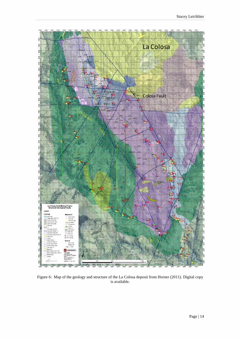
Figure 6: Map of the geology and structure of the La Colosa deposit from Horner (2011). Digital copy

is available.

Stacey Leichliter

Page | 15

The normal Colosa Fault runs along the Colosa River on the eastern side of the

deposit (Figure 6 and digital copy) (Gil-Rodriguez, 2010 and Horner, 2011). This

fault trends north to northwest and dips to the northeast. There are numerous smaller

faults near the deposit, which strike north to northwest and east to northeast. The

structural study by Horner (2011) concluded that these smaller faults have normal

displacement. The smaller faults were conduits for the mineralised fluids (Lodder et

al., 2010). A high grade zone (> 0.7 g/t) may be related to an, as yet, unidentified

fault system in the centre of the deposit.

3.3 La Colosa Lithologies

The La Colosa porphyry gold deposit is part of a late Miocene porphyry intrusion

cluster (approximately 20 km2) with lithologies that range from diorites to quartz

diorites (Figure 7) (Lodder et al., 2010). The porphyry cluster has intruded basement

metamorphic rocks of the Cajamarca Complex. Photographs of the major lithologies

at La Colosa are in Appendix E.

Cross-cutting relationships are the major basis for the different names for the

intrusions. The intrusive complexes have been categorized into three types: early,

intermineral, and late based on cross-cutting relationships and geology (e.g.

mineralogy, texture, alteration intensity and vein frequency). There are very subtle

mineralogy and texture differences between the early and intermineral diorites. Vein

frequency and alteration intensity are used to also classify these rock types.

Stacey Leichliter

Page | 16

Early Diorite Porphyry

Late Diorite Porphyry

Intermineral Diorite Porphyry

Hornfels

Schist

Planned Pit Design

Deposit Areas

Scale = 1:25,000

Drill Hole Collars

Legend

N

La Colosa

MetamorphicCentral

San Antonio

Designed

Pit

Figure 7: Geologic map from AngloGold Ashanti Colombia geologists showing the planned

production pit and zones within the deposit (AngloGold Ashanti Colombia, 2011).

The late intrusions have different mineralogy and texture (alteration and veining)

from the early and intermineral intrusions. The early diorite forms the oldest

intrusions. They have moderate to strong alteration (potassic, potassic-calcic, or

calcic-sodic) and high vein frequency (up to 25 veins per metre) (Lodder et al., 2010).

Intermineral diorites have weak to moderate alteration (potassic and potassic-calcic)

and low vein frequency (less than 10 veins per metre) (Gil-Rodriguez, 2010 and

Lodder et al., 2010). Late intrusions have quartz phenocrysts and locally have

propylitic alteration (Gil-Rodriguez, 2010).

3.3.1 Hornfels/Schist

The Cajamarca Complex is a suite of low grade metamorphic rocks, including schist,

quartzite, and marble, which formed the core of the Central Cordillera (Maya and

González, 1995; Gil-Rodriguez, 2010). The Cajamarca Complex at the deposit site

includes green and black schists. The schist close to the diorite intrusions was

Stacey Leichliter

Page | 17

metamorphosed into hornfels (Figure 7). The major minerals of the hornfels are

plagioclase, quartz, muscovite, and chlorite (Gil-Rodriguez, 2010 and Lodder et al.,

2010). There is little to no foliation visible in the mineralised parts of the hornfels

(Figure 8). The parent rock of the schist is most likely shale. The dominant

alteration assemblage for the hornfels unit is potassic with K feldspar (orthoclase),

pyrite, and biotite (this study). The average gold grade in the hornfels is less than 0.5

g/t and appears to be associated with veins and faults according to detailed AGA

logging.

Figure 8: Altered hornfels from AGA Colombia Logging Manual (1 bar = 1 cm).

3.3.2 Early Diorites

The early diorites have multiple phases (E0, E1, E2, and E3) with two intrusive

breccias (EBX1 and EBX2). A possible fifth early diorite phase (EDM) has been

identified. The early diorite phases have the highest grades of gold (>1 g/t) with

stockwork veinlets (> 25 veins per metre) and potassic, potassic-calcic, and calcic-

sodic alteration assemblages (Lodder et al., 2010).

The earliest intrusion is E0 (Figure 9). It has a very fine-grained matrix of

plagioclase, amphibole, and quartz. Plagioclase and amphibole phenocrysts (0.2 mm

Stacey Leichliter

Page | 18

- 2 mm) form approximately 50% of the rock (Gil-Rodriguez, 2010). The

predominant alteration is potassic with biotite replacing amphibole and plagioclase.

Figure 9: Early diorite E0. COL112_266-268.

The next intrusion, based on cross-cutting relationships and texture, is E1 or the

“crowded” diorite porphyry (Figure 10) (AGA Colombia Logging Manual). It is

medium to fine-grained with phenocrysts up to 5 mm across. The matrix is mainly

quartz and feldspar. Other minerals visible are plagioclase, amphibole, quartz, and

biotite (Gil-Rodriguez, 2010). The dominant alteration is potassic with biotite

(phlogopitic) replacing the other ferromagnesian minerals and K feldspar replacing

plagioclase in the matrix and especially in the vein halos.


Stacey Leichliter

Page | 19

Intrusion breccia EBX1 has clasts of E1 in a medium to very fine-grained matrix

(Figure 11). This intrusive breccia is not a common rock compared to the later

intrusive phases. The major minerals are plagioclase, amphibole, K feldspar

(orthoclase), and quartz. Accessory minerals include apatite, zircon, and sphene (Gil-

Rodriguez, 2010). The dominant alteration is potassic with similar textures to E1.

Figure 11: EBX1 from the AngloGold Ashanti Colombia Logging Manual (1 bar = 1 cm).

The E2 unit is a medium to coarse-grained diorite porphyry with approximately 40%

phenocrysts (Figure 12). The fine-grained matrix is composed of plagioclase,

amphibole, and quartz. The phenocrysts (approximately 5 mm) are plagioclase,

amphibole, and quartz. The dominant alteration type is potassic-calcic with minor

(2% - 5%) actinolite, quartz along fractures, biotite (phlogopitic) rims on the

amphibole phenocrysts, and disseminated pyrite (possibly associated with actinolite).

Stacey Leichliter

Page | 20


The second intrusion breccia unit, EBX2, contains fragments of E2 in a very fine-

grained matrix of plagioclase, amphibole, and quartz (Figure 13). They range from

fine to coarse-grained (Gil-Rodriguez, 2010). Dominant alteration assemblages are

potassic and potassic-calcic. Amphibole phenocrysts are altered to biotite

(phlogopitic) and the plagioclase phenocrysts are altered to K feldspar. The potassic-

calcic traits are similar to those in E2.

Figure 13: EBX2 from AngloGold Ashanti Colombia Logging Manual (1 bar = 1 cm).

Early diorite unit, E3, is a fine-grained diorite porphyry with a groundmass composed

of quartz, plagioclase, K feldspar, and amphibole (Figure 14). Phenocrysts are

plagioclase and amphibole (< 3.5 mm) with an abundance of approximately 20% (Gil-

Rodriguez, 2010). The dominant alteration type is potassic with biotite replacing the

Stacey Leichliter

Page | 21

other ferromagnesian minerals and K feldspar replacing plagioclase. Disseminated

pyrite and chalcopyrite are spatially associated with biotite.


The latest discovery in early diorite porphyries is named EDM, or early diorite

medium-grained (Figure 15). It is medium-grained with phenocrysts of plagioclase

and minor amphibole. Phenocryst abundance is about 50%. The groundmass is

comprised of plagioclase and quartz. EDM is pervasively altered with potassic,

potassic-calcic, and zones with sericite overprinting the earlier alteration assemblages.

This lithology has lower gold grades, but higher, though still uneconomic, copper and

molybdenum grades.

Figure 15: Early diorite EDM. COL112_564-566.

Stacey Leichliter

Page | 22

3.3.3 Intermineral Diorites

The intermineral diorite units in the La Colosa deposit are similar in texture and

composition to the early diorite units, although the intermineral diorites appear to

contain fewer veins. There are two phases (I1 and I2) and an intrusive breccia (IBX)

(AngloGold Ashanti Colombia Logging Manual). The dominant alteration

assemblages are potassic and potassic-calcic. The average gold grade of the

intermineral diorites is < 0.8 g/t.

Intermineral unit I1 has a matrix of plagioclase, amphibole, and quartz (Figure 16).

The phenocrysts are plagioclase, amphibole, and quartz (approximately 5 mm) and

about 20% abundance (Gil-Rodriguez, 2010). The dominant alteration assemblages

are potassic and potassic-calcic with amphiboles altering to actinolite and biotite.

Figure 16: Intermineral diorite I1. COL101_274-276.

The intrusive breccia unit IBX is composed of fragments of I1 in a very fine- to fine-

grained matrix of plagioclase, amphibole, and quartz (Figure 17). The phenocrysts

constitute approximately 30% of the rock and are plagioclase, amphibole, and quartz

(< 6 mm) (Gil-Rodriguez, 2010). Potassic and potassic-calcic are the major alteration

assemblages with plagioclase and amphibole altering to biotite and actinolite.

Stacey Leichliter

Page | 23

Figure 17: IBX from AngloGold Ashanti Colombia Logging Manual (1 bar=1 cm).

The second intermineral unit, I2, is a diorite porphyry with a very fine-grained matrix

of plagioclase, amphibole, and quartz (Figure 18). The plagioclase, amphibole, and

quartz phenocrysts (40%) are fine to medium grained (< 5 mm) (Gil-Rodriguez,

2010). The dominant alteration type is potassic with plagioclase and amphiboles

altering to biotite.

Figure 18: Intermineral diorite I2 from AngloGold Ashanti Colombia Logging Manual (1 bar=1 cm).

3.3.4 Late “Dacites” and Quartz Diorites

The late units include “dacites” and quartz diorites. The “dacite” unit is named using

field observations but is chemically a quartz diorite (Gil-Rodriguez, 2010). These

units have little to no gold, except along contacts with other intrusions, and average

Stacey Leichliter

Page | 24

less than 0.5 g/t gold. Intermediate argillic and propylitic alteration assemblages are

dominant.

The dacite or late diorite porphyry unit in Figure 16 is the largest body of this group.

It forms a stock with a diameter of 1.6 km in the north to northeastern part of the

deposit. It has a very fine-grained matrix of plagioclase, amphibole, biotite, and

quartz (Figure 19). Plagioclase, quartz, biotite, and amphibole phenocrysts

(approximately 30%) are fine to coarse-grained (< 1 cm) (Gil-Rodriguez, 2010). The

predominant alteration type is propylitic with amphibole altering to chlorite.

Figure 19: Weakly altered “dacite”. COL028_204-206.

There is a late quartz diorite stock located in the eastern side of the deposit (Gil-

Rodriguez, 2010). It is of similar composition to the late dacite stock mentioned

above. The quartz diorite is also barren, except along contacts with the earlier

diorites. The dominant alteration is propylitic with trace potassic alteration observed

in the contacts.

There are numerous dacite and quartz diorite dikes that strike northwest in the

northern and central parts of the deposit and cross-cut the hornfels, early, and

intermineral diorite units (Gil-Rodriguez, 2010). These dikes have similar

Stacey Leichliter

Page | 25

composition and texture to the dacite and quartz diorite porphyries listed above. The

alteration assemblage is propylitic, and the gold grade is restricted to the contacts with

the other lithologies, such as hornfels, early diorites, and intermineral diorites.

3.4 La Colosa Alteration

3.4.1 Alteration Assemblages

The alteration assemblages present at the La Colosa gold porphyry deposit include

potassic-calcic, potassic, calcic-sodic, quartz-sericite, intermediate argillic, and

propylitic. Terminology for the alteration assemblages is taken from the geologic

logging manual at La Colosa (AngloGold Ashanti Colombia Logging Manual), and

this study expands and confirms the previous work. Dominant alteration assemblages

are potassic and potassic-calcic (Lodder et al., 2010). There are minor abundances of

calcic-sodic, quartz-sericite, intermediate argillic and propylitic alteration present as

well (Lodder et al., 2010). Potassic and potassic-calcic alteration may be overprinted

with the calcic-sodic or quartz-sericite alteration. Photographs of the various

alteration assemblages are located in Appendix E (digital).

3.4.2 Potassic

The potassic alteration is characterized by fine-grained, hydrothermal biotite replacing

the ferromagnesian phenocrysts, secondary biotite replacing the groundmass, K

feldspar (hydrothermal) replacing the plagioclase in phenocrysts and groundmass

(Gil-Rodriguez, 2010). It can be pervasive in the groundmass or as vein halos. The

assemblage is phlogopitic biotite + K feldspar + magnetite + quartz + sulfides (Figure

20). Early biotite, magnetite, and quartz-sulfide veins are related to this alteration

assemblage (Gil-Rodriguez, 2010, this study).

Stacey Leichliter

Page | 26

Figure 20: Potassic alteration (strong) in EBX2. COL062_222-224.

3.4.3 Potassic-Calcic

The potassic-calcic alteration assemblage is similar to the potassic alteration but

includes actinolite (Gil-Rodriguez, 2010 and this study). It can be pervasive in the

groundmass, or as patches and vein halos. The alteration assemblage is K feldspar +

phlogopitic biotite + albite/oligoclase + actinolite + magnetite + quartz + sulfides

(pyrite) (Figure 21).

Figure 21: Potassic-calcic alteration in EBX1. COL108_54-56.

3.4.4 Calcic-Sodic

At La Colosa, the albite and actinolite alteration minerals dominate calcic-sodic

alteration (Gil-Rodriguez, 2010 and this study). This alteration assemblage overprints

potassic or potassic-calcic alteration in some zones (Figure 22). The overprinting is

Stacey Leichliter

Page | 27

patchy in areas (albite). The veins associated with the sodic-calcic alteration are

similar to the potassic, but also include actinolite and albite or low calcium

plagioclase in the vein assemblage (Gil-Rodriguez, 2010 and AngloGold Ashanti

Colombia Logging Manual).

Figure 22: Calcic-sodic alteration overprinting potassic alteration COL062_126-128.

3.4.5 Quartz-Sericite

The quartz-sericite alteration assemblage includes sericite (fine-grained white mica),

fine-grained pyrite, and quartz (Figure 23) (Gil-Rodriguez, 2010). This assemblage

locally overprints the potassic and potassic-calcic alteration assemblage. Quartz and

sericite (white mica) occur as vein halos and replacement of the groundmass. Quartz-

sulfide veins with quartz-sericite halos are related to this alteration.

Figure 23: Quartz-sericite alteration overprinting potassic alteration in hornfels. COL111_582-584.

Stacey Leichliter

Page | 28

3.4.6 Intermediate Argillic

The intermediate argillic alteration assemblage includes illite, chlorite, and sericite

and locally overprints other alteration assemblages, such as potassic and potassic-

calcic (AngloGold Ashanti Colombia Logging Manual). This assemblage destroys

the original texture of the rock.

3.4.7 Propylitic

The propylitic alteration assemblage includes chlorite, epidote, and calcite (Figure 24)

(Gil-Rodriguez, 2010, AngloGold Ashanti Colombia Logging Manual). This

alteration is observed in some of the intermineral diorites and in the late dacite

porphyry on the edge of the deposits. The chlorite replaces some phenocrysts and can

also occur as veins. Chlorite is the preferred indicator mineral for the assemblage,

because epidote is abundant in all the diorites. There is a moderate correlation

between the chlorite alteration and copper mineralisation. Chlorite veins are

associated with this alteration assemblage.

Figure 24: Propylitic alteration (chlorite and epidote) in I1. COL101_252-254.

3.5 La Colosa Vein Types

The vein types found at the La Colosa deposit include early biotite (EB), magnetite

(M), quartz-sulfide (A), quartz-sulfide with a banded suture (B), sulfides (S), sulfide-

Stacey Leichliter

Page | 29

quartz with a quartz-sericite halo (D), chlorite, and actinolite veins. These vein names

are derived from the manual for logging at La Colosa (AngloGold Ashanti Colombia

Logging Manual). The most common veins are the quartz-sulfide (A) and sulfides

(S). These vein types have a weak to moderate spatial correlation with the gold

mineralisation. Photographs of the different types of vein are in Appendix E (digital).

3.5.1 Early Biotite

The early biotite veins (EB) have fine-grained biotite and are the earliest recognized

phase of veins (Figure 25). They are associated with the potassic alteration

assemblage. They are thin and sinuous.

Figure 25: Early biotite veins in EBX1. COL069_332-334.

3.5.2 Magnetite

The magnetite veins (M) have magnetite, with or without actinolite, and K feldspar or

albite (Figure 26) (AngloGold Ashanti Colombia Logging Manual, this study). These

veins are irregular, discontinuous, and thin (a few millimetres wide) (AngloGold

Ashanti Colombia Logging Manual, this study). Pyrite is visible in some of the veins.

The M veins are a product of the potassic and potassic-calcic alteration. They are

more prevalent in the northeastern section of the deposit.

Stacey Leichliter

Page | 30

Figure 26: Magnetite vein with feldspar halo in EBX2. COL062_264-266.

3.5.3 Quartz-Sulfide

The quartz-sulfide veins, A, are composed of quartz with K feldspar, sulfides (pyrite,

chalcopyrite, bornite, and molybdenite), oxides (magnetite) or only quartz (Figure 27)

(AngloGold Ashanti Colombia Logging Manual). The veins are continuous and

sinuous with or without a halo of alteration and range from thin (< 5 mm) to wide (>

10 cm) (AngloGold Ashanti Colombia Logging Manual and this study). The A veins

form in the potassic alteration zone and appear as stockwork in highly mineralised

zones. There are steeply dipping and shallower dipping vein orientations. Both vein

orientations are cross cut by other quartz veins in a stockwork pattern. The A veins

have a weak to moderate correlation with gold in the eastern and central section of the

deposit. These veins are typical of gold porphyry deposits (Sillitoe, 2000).

Figure 27: Quartz-magnetite-sulfide vein in IBX. COL062_432-434.

Stacey Leichliter

Page | 31

3.5.4 Quartz-Sulfide with Suture

The quartz-sulfide veins with a suture, B, are similar to the A veins, but have a central

band of sulfides (Figure 28) (AngloGold Ashanti Colombia Logging Manual). These

veins are more continuous than the A veins and are tens of millimetres wide

(AngloGold Ashanti Colombia Logging Manual, this study). They occur in the

potassic alteration zone. These veins are rare in the deposit. No spatial correlation

with the gold mineralisation has been detected. The B veins are more typical of

molybdenum porphyry deposits (Sillitoe, 2000).

Figure 28: Quartz-sulfide with suture in EDM. COL099_198-200.

3.5.5 Sulfide

The sulfide veins (S) contain pyrite, pyrrhotite, and chalcopyrite (Figure 29)

(AngloGold Ashanti Colombia Logging Manual and this study). They locally have an

alteration halo and are up to a few centimetres wide (AngloGold Ashanti Colombia

Logging Manual and this study). The S veins include both discontinuous and

continuous veins (AngloGold Ashanti Colombia Logging Manual and this study).

Cross-cutting relationships indicate there are multiple phases of sulfide veins. The

veins are spatially related to potassic and quartz-sericite alteration. These veins are

Stacey Leichliter

Page | 32

typical of porphyry gold deposits (Sillitoe, 2000). Sulfide veins have a weak to

moderate spatial correlation with gold mineralisation.

Figure 29: Sulfide vein in E0. COL112_300-302.

3.5.6 Sulfide-Quartz

The sulfide-quartz veins (D) have a quartz-sericite halo (Figure 30) (AngloGold

Ashanti Colombia Logging Manual). They are a minor vein type associated with the

quartz-sericite alteration (AngloGold Ashanti Colombia Logging Manual and this

study). These veins can be up to 5 cm wide and have a vuggy texture (AngloGold

Ashanti Colombia Logging Manual and this study). The quartz-sericite halos are up

to 10 cm wide. Some D veins contain gold.

Figure 30: Sulfide-quartz vein with quartz-sericite alteration halo in EBX2. COL062_126-128.

Stacey Leichliter

Page | 33

3.5.7 Chlorite and Actinolite

Chlorite veins are found in areas of propylitic alteration and are thin (< 5 mm)

(AngloGold Ashanti Colombia Logging Manual and this study). The chlorite veins

can have a central sulfide suture and a feldspar alteration halo (AngloGold Ashanti

Colombia Logging Manual and this study). Actinolite veins are spatially associated

with potassic-calcic alteration and are also thin (Figure 31). The actinolite veins have

variable sulfide content.

Figure 31: Actinolite-sulfide vein with feldspar alteration halo in EBX1. COL069_352-354.

3.6 Summary

The La Colosa porphyry gold deposit occurs within a cluster of multiple porphyritic

intrusions (Lodder et al., 2010). The structural setting, with major normal faults

striking northwest and conjugate normal faults striking northeast, reflects the regional

structure (Gehrels, 2008 and Lodder et al., 2010). The normal faults are thought to be

the conduits for the intrusions and mineralised fluids which formed the porphyry

system. There are seven phases of early diorite, which hosts the majority of the gold

mineralisation (Lodder et al., 2010). The intermineral diorites have three phases and

contain lower gold grades (Lodder et al., 2010). The late dacites and quartz diorites

occur as stocks or dikes striking northwest and are mainly barren (Lodder et al.,

Stacey Leichliter

Page | 34

2010). The mineralisation of the deposit is associated with potassic alteration which

may be overprinted in areas by calcic-sodic and quartz-sericite alteration (Lodder et

al., 2010).

The La Colosa porphyry gold deposit has many of the typical alteration and vein types

associated with other porphyry copper-gold and porphyry gold systems (Sillitoe,

2007). Recognising the potassic alteration in the hornfels has been difficult at the site

but is apparent in mineralogical analyses. The presence of potassic alteration, lack of

a lithocap, and the lack of a prominent propylitic halo may indicate the system is at a

deeper zone in the deposit model (Seedorff et al., 2008). It also may indicate a

circulation of both magmatic and meteoric waters (Seedorff et al., 2008). There are

multiple phases of the potassic alteration coinciding with the many intrusions, which

also links with the multiple generations of quartz-sulfide and sulfide veins. The

presence of multiple fluid pulses suggests there may also be multiple phases of gold

mineralisation.

Stacey Leichliter

Page | 35

Chapter 4: Review of Porphyry Copper-Gold

and Porphyry Gold Deposits

4.1 Introduction

According to Sillitoe (2010), porphyry copper systems are defined as hydrothermally

altered rock in large volumes (10 km3

- 100 km3) which are centred on porphyry

intrusions. La Colosa is a deposit with a cluster of porphyritic intrusions that are

hydrothermally altered with a high concentration of gold and weaker amounts of

copper and molybdenum. Both porphyry copper-gold and porphyry gold systems will

be described for their different types of copper, gold, and molybdenum mineralisation.

Their traits were used to develop the model for La Colosa.

Previous works, including references to gold porphyry deposits, are Gustafson and

Hunt (1975); Vila et al (1991); Muntean et al (2000); Sillitoe (2000); Ulrich and

Heinrich (2002); Proffett (2003); Redmond and Einaudi (2010); and Sillitoe (2010).

These works and reports were concentrated on porphyry copper, porphyry copper-

gold, and porphyry gold deposits and their models. Different models and detailed

descriptions of the deposits similar to La Colosa aid in the understanding of the

paragenesis and gold mineralisation.

4.2 Terminology

The descriptive terminology of the porphyry copper-gold and porphyry gold deposits

was originally developed by Gustafson and Hunt (1975) and Sillitoe (2000). The

terminology describes the lithologies, alteration assemblages, and vein types, which

are similar between the porphyry copper-gold and porphyry gold deposits. The

Stacey Leichliter

Page | 36

lithologies are calc-alkaline or alkaline intrusions, both of which can be felsic to

intermediate in composition. The gold-rich porphyries tend to occur in the more mafic

rocks. Porphyry copper-gold deposits have multiple phases of intrusions which are

named for their relationship to the timing of the mineralisation: early (before

mineralisation), intermineral (during mineralisation), and late (after mineralisation).

The early porphyries typically host the majority of the mineralisation. The

intermineral porphyries have less mineralisation, and the late porphyries are usually

barren or low grade.

There may be a lithocap, or zone of advanced argillic alteration, above the porphyry.

The different types of alteration assemblages associated with porphyry deposits are

calcic-sodic (albite/oligoclase, actinolite, and magnetite); potassic (biotite and

potassic feldspar); propylitic (chlorite, epidote, albite, and carbonate); chlorite-sericite

(chlorite, sericite/illite, and hematite); sericite/phyllic (quartz and sericite); and

advanced argillic (quartz (vuggy), alunite, prophyllite, dickite, and kaolinite) (Sillitoe,

2000 and Sillitoe, 2010).

The different types of veins observed in the porphyry deposits were described by

Gustafson and Hunt (1975). Here are the vein type names in parentheses with the

minerals that form them: magnetite with or without actinolite (M type); early biotite

(EB); granular quartz with sulfides (A type); granular quartz with sulfides and a

central suture (B type); crystalline sulfide with crystalline quartz with a quartz-sericite

halo (D type); early dark micaceous (EDM); and sulfide (S type) (Figure 7) (Sillitoe,

2000 and Sillitoe, 2010).

Stacey Leichliter

Page | 37

4.3 Porphyry Copper-Gold Deposit Models

4.3.1 Deposit Model

Porphyry copper-gold deposits can occur in various tectonic settings with a majority

occurring in magmatic arc environments above subduction zones, but they can also

occur in postcollisional settings. Host rocks to the deposits are typically dioritic to

granitic in composition and of the I-type magnetite series affiliation. Gold-rich

porphyries tend to occur in the calc-alkaline diorite or quartz diorite porphyries (Vila

and Sillitoe, 1991and Sillitoe, 2010). Porphyry copper-gold systems may occur in

districts of clusters up to 30 km in size and have a wide range of ages. Porphyry

copper-gold deposits tend to be located in the top 4 km of the crust, and their central

stocks connect to a depth of 5 km - 15 km where they meet the parental magma

chamber (Figure 32). In the deep potassic altered zones, the porphyry copper-gold

mineralisation may originate straight from a single-phase aqueous liquid with a low

alteration. In the shallower (<4 km) zones of the deposit, the mineralisation is

introduced by a two-phase fluid, brine and vapour (Fournier, 1999 and Sillitoe, 2010).

4.3.2 Alteration and Veining

Porphyry copper-gold deposits have a consistent suite of alteration assemblages. The

alteration assemblages zone upward from sodic-calcic, deep in the base or roots of the

porphyry system, to potassic, chlorite-sericite, sericite (phyllic), and advanced argillic

at shallower levels (Figure 33). The propylitic and chloritic alteration are zoned

distally from the core. The advanced argillic alteration usually appears in the form of

a lithocap, which may be up to 1 km thick (Sillitoe, 2010).

Stacey Leichliter

Page | 38

Figure 32: Telescoped model of a typical porphyry copper-gold system. From Sillitoe (2010) altered

from Sillitoe (1995, 1997, and 2000).

Figure 33: Porphyry copper-gold alteration and mineralisation model from Sillitoe (2010).

The veinlets in porphyry deposits may be grouped into three general categories (their

equivalents are listed by Gustafson and Hunt (1975) terminology): early quartz and

sulfide-free veinlets (actinolite, magnetite (M type), early biotite (EB type) and

potassic feldspar); granular quartz-dominated, sulfide-bearing with no alteration halos

(A and B types); and crystalline quartz-sulfide veinlets and veinlets with feldspar

Stacey Leichliter

Page | 39

destructive halos (D type) (Figure 34). Potassic alteration is associated with the first

two groups of veinlets. The last group is related to argillic alteration with chlorite-

sericite overprints. The bulk of the mineralisation is related to the veins in the second

group and disseminated throughout rocks with potassic alteration (Sillitoe, 2010).

Figure 34: Vein types observed in a porphyry copper-gold deposit from Sillitoe (2010) after Sillitoe

(2000).

4.3.3 Mineralisation

The porphyry deposit usually has two broad zones of mineralisation: supergene and

hypogene. The supergene zone is the oxidised zone, and the hypogene zone is less

oxidised and is usually sulfide rich (Sillitoe, 2010). The mineralisation in porphyry

copper-gold deposit is associated with the potassic alteration assemblages. It is also

associated with the quartz-sulfide-molybdenum-chalcopyrite and sulfide veins. Each

deposit has varying concentrations of copper, gold, and molybdenum (Sillitoe, 2010).

Stacey Leichliter

Page | 40

4.4 Porphyry Copper-Gold Deposits

4.4.1 Bajo de la Alumbrera

The Bajo de la Alumbrera porphyry copper-gold in Argentina shows some similarities

to La Colosa. It is a world-class copper-gold porphyry deposit located 200 km off the

main Andean copper belt of Chile (Ulrich and Heinrich, 2002). It has up to seven

phases of dacitic porphyry intrusions in a cluster which show hydrothermal alteration

and mineralisation (Ulrich and Heinrich, 2002) (Figure 35). The basement rocks in

the district are granites, metasediments, and sedimentary rocks. The host rocks are

the thick andesites and dacites of the Farallon Negro Volcanic Complex.

Figure 35: Geologic map of the Bajo de la Alumbrera deposit from Ulrich and Heinrich (2002) after

Sasso (1997).

The porphyry intrusions show a high calc-alkaline affinity and are similar in texture

to each other (Sasso and Clark, 1998; Ulrich and Heinrich, 2002). They all contain

phenocrysts of plagioclase, hornblende, biotite, and quartz in a quartz-feldspar

groundmass (Proffett, 2003).

Stacey Leichliter

Page | 41

The alteration assemblages include quartz - magnetite ± K feldspar, potassic,

propylitic, and then advanced phyllic and argillic (feldspar destructive). The quartz –

magnetite ± K feldspar assemblage has distinctive fracture fillings and replacement

textures. The potassic alteration has secondary K feldspar in the plagioclase and

groundmass along with shreddy biotite replacing the mafic minerals. The copper and

gold mineralisation is associated with the potassic alteration. The propylitic alteration

(chlorite-epidote) assemblage has chlorite and magnetite replacing mafic minerals and

albite + epidote ± calcite ± sericite replacing plagioclase. The propylitic alteration

surrounds the potassic alteration. The advanced phyllic and argillic (feldspar

destructive) alteration assemblage overprints earlier alteration types and includes

sericite, pyrite, quartz, and rutile with local clay minerals or chlorite ± calcite (Ulrich

and Heinrich, 2002). The alteration zoning is nearly symmetrical, although the

copper-gold mineralisation and veins are less symmetrical and is controlled by

intrusions (Proffett, 2003).

Many of the early veins and quartz veins in the deposit are related to the potassic

alteration assemblage, which tends to occur as halos to the veins. However, the

quartz veins may be without halos or secondary magnetite. The earliest types of veins

are the equigranular quartz with or without magnetite, K feldspar, chalcopyrite,

bornite, biotite, and anhydrite (i.e. A type veins). The next generation of veins is the

B type veins or continuous coarser quartz with banding. The sulfide veins are late and

predominantly consist of pyrite or D type veins which are related to the feldspar

destructive alteration (Proffett, 2003).

Stacey Leichliter

Page | 42

The gold and copper mineralisation usually has a positive correlation with one

another. The copper mineralisation includes chalcopyrite, bornite and covellite. Gold

is associated with these copper sulfides, pyrite, tellurides, or occurs as native gold.

The paragenesis of the deposits suggests two pulses of Fe-K-Cu-Au fluids and a late

post ore fluid pulse (Ulrich and Heinrich, 2002).

4.4.2 Bingham Canyon

The Bingham Canyon porphyry copper-gold-molybdenum deposit is the seventh

largest copper deposit (28 Mt) and the second largest based on gold (1,600 t) in the

world (Redmond and Einaudi, 2010). It is centred on the Eocene monzonite intrusion

called the Bingham stock, which intruded the Pennsylvanian Oquirrh Group quartzite

and limestone (Redmond and Einaudi, 2010). The Bingham stock was intruded by

multiple porphyry dikes including quartz monzonite porphyry, latite porphyry, biotite

porphyry, quartz latite porphyry breccia, and quartz latite porphyry (Redmond and

Einaudi, 2010) (Figure 36). The porphyry intrusions are felsic with phenocrysts of K

feldspar, plagioclase, hornblende, and biotite. The highest copper and gold grades are

located within the quartz monzonite porphyry (early intrusion) (Redmond and

Einaudi, 2010).

The dominant alteration assemblage at Bingham Canyon is potassic and includes an

intensive quartz-K feldspar alteration (Redmond and Einaudi, 2010). The potassic

alteration ranges from weak, which is biotisation of hornblendes and matrix

preservation, to strong, which has vuggy quartz and feldspar with the matrix texture

obliterated. The potassic alteration intensity is also a function of A type veinlet

abundance (Redmond and Einaudi, 2010).

Stacey Leichliter

Page | 43

Figure 36: Geologic and structural map of the Bingham Canyon deposit from Redmond and Einaudi

(2010).

The vein sequence, in order, for the Bingham deposit is early biotite veinlets,

followed by early dark micaceous (EDM) veins, A type quartz veins (potassic

alteration), quartz-molybdenite veins, and quartz-sericite-pyrite veins (Redmond and

Einaudi, 2010). The early biotite veinlets are composed of medium-brown biotite

with no magnetite. The EDM veins are unfilled fractures with halos, where

plagioclase is replaced by andalusite, biotite, sericite, and K feldspar. The EDM veins

contain minor amounts of bornite with or without digenite and chalcopyrite. The A

type quartz veins are the most abundant and are composed of quartz, digenite, bornite,

chalcopyrite, and molybdenite. The gold grade correlates with copper in the bornite-

digenite zones (Redmond and Einaudi, 2010). The A type veins occur in all porphyry

intrusions but have greater concentrations in the quartz monzonite porphyry. The late

quartz-molybdenite veins are composed of euhedral quartz with a vuggy centreline at

elevations above 1,500 m and may contain trace chalcopyrite. The D type veins or

Stacey Leichliter

Page | 44

pyrite veins with quartz-sericite-pyrite halos are located along strike to the northeast

and southeast and at elevations higher than 3,000 m (Redmond and Einaudi, 2010).

The observed relationships between the porphyry contacts and the veins suggest that

each porphyry intrusion event has a sequence of potassic alteration and vein

formation, which are associated with the copper and gold deposition (Redmond and

Einaudi, 2010). Each porphyry has many A type veins, strong potassic alteration, and

high grade copper-gold zones. It is suggested that the mineralisation formed due to a

flux of magmatic-hydrothermal fluids with decreasing amounts of copper and gold as

intrusions occurred due to the depletion of metals and volatiles in the underlying

parent magma chamber (Redmond and Einaudi, 2010). The A type veins and sulfides

represent the pulses of hydrothermal fluid associated with each porphyry intrusion

(Redmond and Einaudi, 2010).

4.5 Porphyry Gold Deposit Models

4.5.1 Deposit Model

Gold-rich porphyry or porphyry gold deposits contain an average gold content of

more than 0.4 g/t (Sillitoe, 2000). These porphyry systems are thought to be a part of

a continuum of systems that range from copper plus gold through gold plus copper to

gold-only porphyry systems (Sillitoe, 2000). Some noted gold-rich porphyries

include Grasberg and the Maricunga belt in Chile (Sillitoe, 2000). Many gold-rich

deposits are formed at convergent plate boundaries during or immediately after

subduction of oceanic crust and can be associated with back-arc settings or

subduction-related volcanoplutonic arcs (Sillitoe, 2000). They are generally formed

in shallow levels of the crust (1-2 km). Structural settings can range from major fault

Stacey Leichliter

Page | 45

zones to minor structures. Gold-rich porphyry intrusions belong to I-type magnetite

series suites (Sillitoe, 2000). The compositions of the porphyry intrusions range from

low potassic calc-alkaline diorite, quartz diorite, and tonalite to high potassic calc-

alkaline quartz monzonite to alkaline monzonite to syenite. All porphyries contain

feldspar and mafic minerals with or without quartz phenocrysts in an aplitic to fine-

grained groundmass (Sillitoe, 2000). The phases are texturally and compositionally

similar, so it is difficult to distinguish between them by appearance (Sillitoe, 2000).

4.5.2 Alteration and Veining

There are six broad alteration assemblages associated with gold-rich porphyries

(Sillitoe, 2000). They are Ca-Na (calcic-sodic) silicate, K silicate (potassic),

propylitic, intermediate argillic, sericitic (phyllic), and advanced argillic (Figure 37).

The Ca-Na silicate contains amphibole (actinolite or hornblende), albite or oligoclase,

and magnetite. It can appear as pervasive replacement or veinlets (Sillitoe, 2000). K

silicate (potassic) alteration has biotite (phlogopitic), K feldspar, quartz (veinlets),

magnetite, and sulfides (chalcopyrite and pyrite) (Sillitoe, 2000). Propylitic alteration

contains chlorite, epidote, calcite, albite, actinolite, and magnetite and is found as the

outer halos of the deposit. The intermediate argillic alteration is an overprint to K

silicate assemblages and contains sericite, illite, chlorite, calcite, and smectite.

Sericite (phyllic) alteration may also overprint the K silicate alteration as a white to

gray quartz-sericite-pyrite assemblage. The advanced argillic alteration is found in

the upper sections of the deposits where it forms lithocaps as thick as 1 km (Sillitoe,

2000).

Stacey Leichliter

Page | 46

Figure 37: Model of a porphyry gold deposit from Sillitoe (2000).

A variety of vein types can be found in gold-rich porphyries. They include early

magnetite (M type), early biotite (EB type), vitreous quartz-magnetite-chalcopyrite (A

type), quartz with a central suture (B type), chlorite-pyrite, and quartz-pyrite (D type)

(Figure 38) (Sillitoe, 2000). Early magnetite (M type) veinlets are related to Ca-Na

silicate alteration. Early biotite (EB type) veinlets are found with the K silicate

(potassic) alteration. The A and B type veinlets are also associated with K silicate

(potassic) alteration, but there are usually more A type veinlets present (Sillitoe,

2000). The chlorite-pyrite veins are associated with propylitic alteration. D type

veinlets are related to the sericite (phyllic) alteration. Gold mineralisation is usually

compared with the abundance of A type veinlets (Sillitoe, 2000).

4.5.3 Mineralisation

The gold mineralisation is introduced with copper during the K silicate (potassic)

alteration (Sillitoe, 2000). The gold grades tend to increase with depth. The gold

grain size is commonly < 20 µm or < 100 µm, or fine-grained, and has a fineness

Stacey Leichliter

Page | 47

(ratio of gold to silver content) of > 800 (Sillitoe, 2000). Half the gold may be

associated with pyrite in sulfide-rich deposits. Gold tellurides may be present in

minor amounts. Most gold porphyry deposits are deficient in molybdenum (Sillitoe,

2000).

Figure 38: Vein types observed in porphyry gold deposits from Sillitoe (2000).

4.6 Porphyry Gold Deposits

4.6.1 Marte

Marte is a porphyry gold deposit located in the Andean Cordillera of the Atacama

Region of Chile (Figure 39) (Vila et al., 1991). It is located on the southeastern flank

of the Pastillitos stratovolcano in diorite porphyries divided into three units: coarse-

grained diorite, fine-grained diorite, and microdiorite (Vila et al., 1991). Coarse and

fine-grained diorites are composed of plagioclase, hornblende, biotite, and magnetite

(Vila et al., 1991). The microdiorite is an intrusion breccia with scarce plagioclase

phenocrysts and a salt and pepper textured matrix. The coarse and fine-grained

diorites were subjected to the main alteration assemblages (Vila et al., 1991).

Stacey Leichliter

Page | 48

Figure 39: Geologic map of the Marte deposit from Vila et al. (1991).

The deposit has three main alteration types: advanced argillic, intermediate argillic,

and chlorite (Vila et al., 1991). Advanced argillic alteration occurs at the upper parts

of the deposit and forms a lithocap. This alteration includes chalcedonic quartz,

alunite, and kaolinite with minor amounts of diaspore and rutile. Pyrite appears as

coatings on fractures (Vila et al., 1991). The intermediate argillic alteration includes

hydrothermal quartz, sericite, chlorite, clay (kaolinite), gypsum, hematite, magnetite,

and pyrite. The argillic alteration is thought to have overprinted and obliterated the K

silicate (potassic) alteration. Stockwork quartz veinlets are associated with K silicate

(potassic) alteration. The chlorite alteration includes chlorite, quartz, pyrite, and

hematite with minor amounts of magnetite, chalcopyrite, and molybdenite and affects

the microdiorite (Vila et al., 1991).

The stockwork veinlets at Marte are composed of banded transparent, white, and

black hydrothermal quartz. Black quartz appears as marginal bands or central sutures

and is rich in sulfides. Pyrite is the principal sulfide found in the quartz veinlets (Vila

et al., 1991).

Stacey Leichliter

Page | 49

The gold mineralisation is thought to be present in the quartz stockwork veinlets, and

the gold grade is related to veinlet abundance (Vila et al., 1991). Gold grains range

from 2 µm to 15 µm and classified as very fine. Coarser gold occurs immediately

under the lithocap. The gold is low in silver with an Ag/Au ratio of 0.44. The

average molybdenum content can be as high as approximately 46 ppm (Vila et al.,

1991).

4.6.2 Refugio District (Verde and Pancho)

The Refugio district porphyry gold deposits (Verde and Pancho) are located in the

Maricunga belt in Chile. The Refugio deposits consist of andesitic-dacitic flows and

breccias, dacite porphyry stock, and quartz diorite porphyry stock and breccias

(Figure 40) (Muntean and Einaudi, 2000). The phenocryst composition of the stocks

and intrusions is plagioclase, hornblende, biotite, magnetite, quartz, and augite.

Figure 40: Geologic map of the Refugio district (Verde and Pancho) from Muntean and Einaudi

(2000).

Stacey Leichliter

Page | 50

In the Verde deposit, the gold is associated with the quartz diorite porphyry and

intrusive breccia (Muntean and Einaudi, 2000). The alteration assemblages include

chlorite-magnetite-albite, pyrite-albite-clay, and quartz-K feldspar-chlorite types. The

chlorite-magnetite-albite alteration occurs with the intrusive centre and has gold

grades of > 0.5 ppm (Muntean and Einaudi, 2000). Chlorite and magnetite replace the

mafic phenocrysts. Calcite occurs at the margins of these zones.

Andradite-chlorite-magnetite veinlets are associated with the chlorite-magnetite-albite

alteration assemblages. The pyrite-albite-clay alteration appears in the outermost

zone of the deposit. It consists of limonite, albite, illite, and kaolinite (Muntean and

Einaudi, 2000). The zone is characterised by the absence of magnetite and chlorite. It

also contains 2% - 4% volume pyrite. The quartz-K feldspar-chlorite alteration

occurs in the intrusive breccias. There is a lack of sulfides and iron oxides in the

alteration (Muntean and Einaudi, 2000).

Vein types at the Verde deposit include andradite-chlorite-magnetite and banded

quartz veins (Muntean and Einaudi, 2000). The andradite-chlorite-magnetite veins

are minor in the central parts of the chlorite-magnetite-albite zone but increase in

abundance in the calcite-bearing zones. These veinlets do not appear to have any

correlation with gold. The banded quartz veinlets consist of fine-grained quartz and

sulfides. Pyrite, calcite, K feldspar, sphene, magnetite, and chlorite are found in the

vugs at the centre of the veins. These veins are associated with gold mineralisation

(Muntean and Einaudi, 2000).

Stacey Leichliter

Page | 51

The Pancho deposit is centred on a quartz diorite porphyry stock (Muntean and

Einaudi, 2000). Alteration types include pyrite-albite-clay, tourmaline-bearing pyrite-

albite-clay, potassic alteration (magnetite-K feldspar-oligoclase), potassic alteration

(secondary biotite), and propylitic. The potassic magnetite-K feldspar- oligoclase

alteration is located in the central zone of the deposit. Mafic mineral phenocrysts are

altered to magnetite, oligoclase, quartz, and shreddy biotite. Patches of K feldspar

and quartz replace oligoclase groundmass. The potassic biotite zone is on the flanks

and underneath the potassic magnetite-K feldspar-oligoclase alteration zone. Shreddy

biotite replaces hornblende and biotite. The pyrite-albite-clay alteration overprints the

potassic alterations at high elevations. Kaolinite, quartz, and illite replace the altered

plagioclase or albite phenocrysts (Muntean and Einaudi, 2000).

The vein types at Pancho include A type veins, banded quartz veins (B type), and

pyrite-quartz-sericite veins (D type) (Muntean and Einaudi, 2000). A type veins are

quartz-magnetite-sulfide veinlets and are related to potassic alteration. The banded

quartz veins (B type) are similar to those at Verde but are more abundant. The pyrite-

quartz-sericite (D type) veins are associated with the potassic and pyrite-albite-clay

alteration zones. They can have a vuggy appearance and can contain 10%-60% pyrite

(Muntean and Einaudi, 2000).

The gold grades between 0.5 ppm and 1 ppm at Pancho and coincides with potassic

alteration and A type veins (Muntean and Einaudi, 2000). Higher gold grades (> 1

ppm) are associated with sets of banded quartz veinlets (B type) and magnetite-K

feldspar-oligoclase alteration (Muntean and Einaudi, 2000).

Stacey Leichliter

Page | 52

4.7 Summary

The different models associated with porphyry copper-gold and porphyry gold

systems have many similarities including the alteration assemblages and vein types

(Table 1). The alteration assemblage associated with the mineralisation in most

porphyry models is potassic, as seen in Bajo de la Alumbrera, Bingham Canyon,

Pancho, and La Colosa. The vein types generally associated with mineralisation are

the A type for most of these deposits.

Porphyry copper-gold and porphyry gold deposits have differences. A porphyry gold

deposit can have economic levels of copper and still be labelled gold-rich due to the

gold grades, as in Verde and Pancho. In porphyry copper-gold deposits, gold is

usually a by-product when recovering the copper, because the copper mineralisation is

more abundant and easy to recover, which is found at Bajo de la Alumbrera and

Bingham Canyon. The types of alteration and veins observed in the two models vary.

Calcic-sodic alteration can be present in the porphyry gold deposit (Verde and La

Colosa), and actinolite can be present in some of the veins of the porphyry gold

deposits (La Colosa). Porphyry copper-gold deposits generally have little calcic-sodic

alteration. Some deposits have a lithocap, like the Bajo de la Alumbrera and Marte

deposits, where other deposits have very little advanced argillic alteration such as

Bingham Canyon, Verde, Pancho, and La Colosa.

Stacey Leichliter

Page | 53

Deposit Type Structural Setting Basement Rocks Host Rocks Alteration Assemblages Veins Ore Mineralogy Resources

Bajo de la Alumbrera Cu-AuSubduction/

Compression

Granites,

Metasediments, and

Sedimentary Rocks

Andesites and

Dacites

Quartz - Magnetite ± K

feldspar, Potassic,

Propylitic, and Advanced

Phyllic/Argillic

A type, B type, and D

type

Chalcopyrite,

Bornite, Covellite,

Pyrite, Tellurides,

and Native Gold

551 Mt; Avg Cu

= 0.52% and Au

= 0.67 g/t

Bingham Canyon Cu-Au-Mo ExtensionQuartzite and

Limestone

Quartz Monzanites

and Latites

Quartz - K feldspar and

Potassic

EB type, EDM type, A

type, Late Quartz-

Molybdenum, and D

type

Bornite, Digenite,

Chalcopyrite, Gold

and Molybdenite

3.23 Gt; Avg Cu

= 0.88%, Au =

0.0497 g/t, and

Mo = 0.02%

Marte Au-Cu-MoSubduction/

CompressionAndesites Diorites

Advanced Argillic,

Intermediate Argillic, and

Chlorite

Quartz, A type, and D

type

Magnetite, Pyrite,

Chacopyrite, Gold,

and Molybdenite

46 Mt; Avg Au =

1.43 g/t

Verde AuSubduction/

Compression

Granitoids and

VolcanicsQuartz Diorites

Chlorite - Magnetite -

Albite, Pyrite - Albite -

Clay, and Quartz - K

feldspar - Chlorite

B type and Quartz -

Alunite

Magnetite, Gold,

and Pyrite

101 Mt; Avg Cu

= 0.03% and Au

= 0.88 g/t

Pancho AuSubduction/

Compression

Granitoids and

Volcanics

Quartz Diorites,

Intrusive Breccias,

and Aplites

Pyrite - Albite - Clay,

Tourmaline-bearing Pyrite -

Albite - Clay, Potassic, and

Propylitic

A type, B type, and D

type

Chalcopyrite,

Magnetite, Gold,

and Pyrite

68 Mt; Avg Cu =

0.1% and Au =

0.96 g/t

La Colosa Au Transpression Schists

Diorites, Quartz

Diorites, and

Hornfels

Potassic, Potassic-Calcic,

Calcic-Sodic, Propylitic,

and Intermediate Argillic

EB type, M type, A

type, B type, S type, D

type, Chlorite,and

Actinolite

Gold,

Chalcopyrite, and

Magnetite

392.11 Mt; Avg

Au = 0.98 g/t

Table 1: Summary table of the Porphyry Copper-Gold and Porphyry Gold deposits and their comparison with La Colosa (from Vila et al., 1991; Muntean and

Einaudi, 2000; Ulrich and Heinrich, 2002; Proffett, 2003; Redmond and Einaudi, 2010; AngloGold Ashanti, 2010; and Lodder et al., 2010).

Stacey Leichliter

Page | 54

La Colosa has similar alteration assemblages to the porphyry deposits mentioned, such as

potassic, potassic-calcic, calcic-sodic, propylitic, and argillic. The gold mineralisation at

La Colosa is related to the potassic alteration, which agrees with both the porphyry

copper-gold and porphyry gold models. The host rocks of the porphyry gold deposits are

similar to those at La Colosa. The structural setting is somewhat similar to that of the

porphyry gold models. La Colosa has low copper to gold ratios and fine to very fine-

grained gold (< 10 µm) with gold tellurides and gold-silver tellurides present. The style

of gold mineralisation at La Colosa shares more similarities to the porphyry gold model

than the porphyry copper-gold model, because it has very little copper and molybdenum

and local gold mineralisation correlating with the A type veins.

Stacey Leichliter

Page | 55

Chapter 5: Gold Mineralisation

5.1 Introduction

The La Colosa deposit was discovered in 2007 and is only in its pre-feasibility stage.

Previous work on the gold mineralisation at La Colosa is limited. AGA previously

carried out work with SGS (QEMSCAN®) to identify gold grains and their associations.

QXRD analyses were carried out on many samples and are yet to be interpreted.

It has been suggested the gold mineralisation occurs in multiple situations: within

sulfides (pyrite), within or along boundaries of the silicate minerals (quartz and biotite),

and as liberated gold (Lodder et al., 2010). Gold and gold-silver tellurides along with the

native gold were identified by preliminary testwork carried out by AGA. A major aim of

this project is to describe and understand the gold mineralisation at La Colosa.

5.2 Methods

5.2.1 Introduction

The study on La Colosa’s gold mineralogy, associations, and deportment included

detailed logging, cross sections, Quantitative X-ray Diffraction (QXRD) analysis,

Mineral Liberation Analyser (MLA) XMOD (modal mineralogy) method and MLA

SPL_Lt (sparse phase liberation) method. Data from each method was used to determine

the relationships between the gold mineralisation and the mineralogy and geology of the

deposit.

Stacey Leichliter

Page | 56

5.2.2 Sampling and Preparation

For Phase 1 of the study, seventeen samples were selected from the diamond drill core at

the site based on gold grade. Samples with high gold grades were chosen to increase the

probability of locating gold grains for analysis. The samples selected represented the

major lithologies, i.e. early diorite, intermineral diorite, and hornfels, located in the future

production pit. Each sample was photographed and described (logged) for traits

important to the research project and the details are in Appendices D and E. The detailed

logging was based on parameters used by the geologists on site (i.e. types of alteration

and mineralisation) and other details specified for the project. Such parameters included

the different levels and observations of the potassic alteration (i.e. groundmass alteration

of biotite, biotite and K feldspar alteration of groundmass, and K feldspar alteration of

phenocrysts), description of different types of quartz veins (i.e. quartz only, quartz with

sulfides with no halo, quartz with sulfides with a halo, and quartz with molybdenite), and

different types of sulfide veins observed (i.e. sulfide veins with no halo, sulfide veins

with a halo, sulfide with quartz veins with a quartz-sericite halo, and chalcopyrite veins).

These observations were used to determine the gold paragenesis and related alteration

which are integral to the mineralisation.

The samples were crushed to a size of -4.75 mm (coarse rejects from analytical assay

work) and prepared as grain mounts (25 mm diameter). The grain mounts were prepared

in the University of Tasmania lapidary. All seventeen samples were analysed using the

XMOD and SPL_Lt methods of the MLA in order to determine modal mineralogy and

Stacey Leichliter

Page | 57

gold deportment. Further information on the MLA testwork is described in Chapter

5.2.3.2.

In Phase 2 of the study, 50 samples were selected from the intervals the company was

using for their metallurgical variability testwork. The gold grades of these samples

ranged from 0.3 g/t to greater than 2 g/t. Each sample was logged in detail and then

photographed (logs and photos are in Appendices D and E). The locations of the samples

were concentrated in the primary pit and include the following: early diorite,

intermineral diorite, and hornfels. The coarse rejects from the assay laboratory were used

for the sample material. The fines were sieved from the material and discarded, and the

remaining rock was cleaned and dried.

Gold mineralisation at La Colosa occurs in veins and disseminated (vein poor) in the

groundmass. To examine both types of mineralisation, two metre assay intervals of early

diorite and intermineral diorite were subdivided into increments of ten cm. Each ten cm

increment was logged in detail and then photographed (details in Appendices D and E).

The presence and types of veins were described for each ten cm section of drill core.

Each ten cm section was then assayed, and the results compared to the observations. The

coarse rejects from the assay process were then washed and filtered before being

prepared into grain mounts. The grain mounts were analysed using the XMOD and

SPL_Lt methods of the MLA. The data was used to determine any differences between

vein (vein rich) and disseminated (vein poor) gold mineralisation.

Stacey Leichliter

Page | 58

5.2.3 Analysis

5.2.3.1 Deposit Models

Simplified geologic, alteration, and mineralisation models were constructed using data

from AngloGold Ashanti’s drill hole database and detailed geologic logs. Cross sections

were constructed from drill hole logs provided by the company using Leapfrog 3D

imaging software (Leapfrog, 2011) to understand the spatial relationships between

lithology, alteration, vein types, and gold mineralisation. These cross sections were

developed to give a visual representation of the system.

Geological cross sections were utilised to build a model of the deposit and to determine

the spatial location and type of alteration assemblages associated with the gold

mineralisation. Visual drill log data was used to create cross sections in order to ascertain

which vein type was associated with the gold mineralisation. Cross sections were also

used to examine the relationship between gold mineralisation associated with sulfides

versus tellurides.

The QXRD and drill log information was used to understand the mineralogical changes

in the weakly altered (less mineralised), strongly altered (mineralised), or highly

mineralised samples. Drill log information for alteration character is subjective due to

the number of geologists’ interpretations.

Stacey Leichliter

Page | 59

5.2.3.2 MLA Testwork

In order to determine mineralogy, the MLA uses backscattered electron (BSE) images

along with X-ray analysis to identify the mineral. Minerals that have similar energy

intensities in the BSE images need to be differentiated. The grey-scale levels in the BSE

range from 0-255 and are related to the average atomic number of the element (Gu,

2003). A grey-scale of 0 generally indicates epoxy mounting resin whereas a level of 255

is gold (Gu, 2003). Minerals like gold, silver, sulfides, barite and galena appear brighter

in the BSE image, whereas quartz and feldspars appear darker in the BSE image.

Minerals with similar brightness intensities on the BSE image need X-ray mapping from

the spectra to determine their chemistry (Gu, 2003).

MLA’s XMOD method uses a grid of X-ray points determined by the SEM operator to

produce a modal mineralogy (Gu, 2003). In this study it was performed at a

magnification of about 150x. This produces bulk mineralogy of the sample. The XMOD

method from the MLA provides a high quality modal mineralogy. Details of the method

can be found in the report by Gu (2003). Data from the XMOD method was compared to

the QXRD data to observe the enrichments or depletions in the samples.

The SPL_Lt method uses the grey-scale levels in the BSE to locate the mineral of interest

(gold) and then analyse the surrounding area of the sample using X-ray spectra (Gu,

2003). Each mineral of interest is identified and examined with X-ray analysis to

produce particle mineral maps (Gu, 2003). The gold grains were verified by spectra and

Stacey Leichliter

Page | 60

photographed. The SPL_Lt analysis can produce information on the boundaries, grain

sizes, mineral associations, locking and liberation of the mineral of interest.

The SPL_Lt method yielded information on the gold grain boundary, area, grain size

distribution, locking, liberation (recovery), and the phase specific surface area (PSSA).

The PSSA is calculated by dividing the gold grain boundary by the area of the gold grain

(Berry, 2011). The PSSA is a metallurgical term used to describe the gold grain size and

texture.

The PSSA reported by the MLA is not consistent with the 3D grain size analysis (Berry,

2011). The average grain size in each sample was calculated using Berry’s equation

(2011).

Average grain size = 4.7/ (Average PSSA gold grains)

This calculation is volume weighted and includes a correction for complex grain shapes

(Berry, 2011). Edge effects of the bright phases may contribute to an over estimation of

their grain sizes. These edge effects are exacerbated by high voltage, large spot size, and

long working distance (> 10mm).

Data from the MLA analyses is in Appendix F. Note the smallest detectable grain size

for the SPL_Lt method, set at a magnification of 300x, in this study was 0.87 µm. There

is a trade-off with the magnification settings for the MLA a higher magnification has

higher precision and lower detection limit, but the analysis takes longer to perform.

Stacey Leichliter

Page | 61

There is a trade off with a lower magnification, quicker analysis of the XMOD method,

but has less precision and a larger detection limit, but the SPL_Lt method is more

expensive and time consuming.

5.3 Gold Mineralogy

5.3.1 Introduction

The textures and species of the gold mineralogy at the La Colosa deposit were interpreted

from the data produced by the SPL_Lt method of the MLA. There were 148 gold grains,

111 gold telluride grains, and 63 gold-silver telluride grains located and analysed (Tables

2 and 3).

5.3.2 Types of Gold Mineralisation

There were three gold-bearing minerals observed in the La Colosa samples: native gold,

gold tellurides, and gold-silver tellurides (Tables 2 and 3). The deportment of these gold

minerals is described in the following sections (Chapters 5.3.4, 5.3.5, and 5.3.6). The

gold contained small amounts of silver, with only a couple of gold grains with a silver

content high enough to be classified as electrum (Ag wt% 25%-55%) (Table 4). The

average fineness of the gold grains was calculated to be approximately 881, where 1,000

is pure gold. The equation for fineness is (Marsden and House, 2006):

fineness = (Au wt% x 1,000)/ (Au wt% + Ag wt%)

Stacey Leichliter

Page | 62

Sample ID Lithology Au g/t Au grains Au Te grains Au-Ag Te grains

005_42-44 E2 12.00 2 7 0

005_44-46 E2 27.20 1 0 0

005_122-124 E2 8.05 10 5 1

006_84-86 E3 7.12 6 0 0

008_130-132 H 9.50 48 36 0

010_152-154 EBX2 8.59 1 0 0

030_194-196 E2 22.30 7 3 1

033_104-106 H 28.90 7 1 0

034_60-62 E3 22.50 1 1 0

034_378-380 IBX 44.90 3 1 0

035_46-48 EBX2 12.00 2 1 0

036_292-294 H 9.08 1 1 0

040_62-64 E0 7.51 3 2 0

040_114-116 IBX 7.80 6 1 1

041_184-186 H 9.76 0 0 0

046_290-292 IBX 9.09 6 3 0

049_158-160 IBX 29.70 13 42 54

060_77-81 H 2.13 0 0 1

062_126-130 EBX2 0.88 0 0 0

062_224-226 EBX2 0.77 0 0 0

062_406-410 IBX 1.03 4 0 0

064_106-110 E3 0.75 1 0 0

064_160-164 EBX2 1.22 1 0 0

064_176-180 EBX2 0.89 0 0 0

064_328-332 EBX2 0.55 0 0 0

066_108-112 E3 1.55 1 0 0

066_122-126 EBX2 1.00 0 0 0

066_138-142 EBX2 1.25 0 0 0

066_224-228 EBX2 0.91 2 0 0

066_292-296 EBX2 0.69 0 0 0

078_80-83.3 H 1.69 0 0 0

089_74-78 H 1.80 1 0 0

089_180-184 H 0.95 0 0 0

101_110-116 IBX 0.86 0 0 0

101_248-252 I1 0.74 0 0 0

101_258-262 I1 1.90 0 0 0

101_270-274 I1 0.52 0 1 0

101_366-370 I1 1.64 1 0 4

101_488-492 H 2.93 0 0 0

101_524-528 H 3.71 2 0 0

101_576-580 H 0.53 1 0 0

108_74-78 E1 3.24 0 0 0

108_132-136 E1 0.65 0 0 0

108_152-156 E1 0.94 0 0 0

108_164-168 E1 2.07 0 0 0

108_200-204 E1 4.80 1 0 0

108_358-362 IBX 2.59 2 0 0

109_40-44 IBX 4.59 2 0 1

109_250-254 E2 0.43 2 2 0

112_156-160 EBX2 2.33 4 1 0

112_172-176 EBX2 2.20 0 0 0

112_218-222 EBX2 4.36 2 3 0

112_230-234 EBX2 1.71 1 0 0

112_262-266 E0 1.40 0 0 0

112_318-320 E0 1.08 0 0 0

112_356-360 EDM 1.83 1 0 0

112_406-410 EDM 0.85 1 0 0

114_424-428 H 0.92 0 0 0

114_432-436 H 0.75 1 0 0

Total Grains 148 111 63

Avg Au g/t 5.82

Table 2: Summary table for Phase 1 and 2 samples analysed by the SPL_Lt method.

Stacey Leichliter

Page | 63

Sample ID Lithology Au g/t Au grains Avg Au grain size (µm) Au Te grains Avg Au Te grain size (µm) Au-Ag Te grains Avg Au-Ag Te grain size (µm)

005_42-44 E2 12.00 2 2.61 7 6.53 0

005_44-46 E2 27.20 1 6.71 0 0

005_122-124 E2 8.05 10 8.25 5 1.97 1 10.93

006_84-86 E3 7.12 6 4.20 0 0

008_130-132 H 9.50 48 7.58 36 4.52 0

010_152-154 EBX2 8.59 1 8.10 0 0

030_194-196 E2 22.30 7 5.05 3 10.93 1 8.70

033_104-106 H 28.90 7 13.43 1 1.37 0

034_60-62 E3 22.50 1 16.79 1 6.03 0

034_378-380 IBX 44.90 3 5.11 1 16.21 0

035_46-48 EBX2 12.00 2 7.34 1 1.58 0

036_292-294 H 9.08 1 15.16 1 0.77 0

040_62-64 E0 7.51 3 12.05 2 5.40 0

040_114-116 IBX 7.80 6 3.73 1 2.19 1 4.09

041_184-186 H 9.76 0 0 0

046_290-292 IBX 9.09 6 10.22 3 13.82 0

049_158-160 IBX 29.70 13 15.16 42 5.40 54 7.23

060_77-81 H 2.13 0 0 1 1.58

062_126-130 EBX2 0.88 0 0 0

062_224-226 EBX2 0.77 0 0 0

062_406-410 IBX 1.03 4 11.19 0 0

064_106-110 E3 0.75 1 3.20 0 0

064_160-164 EBX2 1.22 1 3.01 0 0

064_176-180 EBX2 0.89 0 0 0

064_328-332 EBX2 0.55 0 0 0

066_108-112 E3 1.55 1 1.82 0 0

066_122-126 EBX2 1.00 0 0 0

066_138-142 EBX2 1.25 0 0 0

066_224-228 EBX2 0.91 2 3.48 0 0

066_292-296 EBX2 0.69 0 0 0

078_80-83.3 H 1.69 0 0 0

089_74-78 H 1.80 1 2.13 0 0

089_180-184 H 0.95 0 0 0

101_110-116 IBX 0.86 0 0 0

101_248-252 I1 0.74 0 0 0

101_258-262 I1 1.90 0 0 0

101_270-274 I1 0.52 0 1 7.46 0

101_366-370 I1 1.64 1 2.13 0 4 1.68

101_488-492 H 2.93 0 0 0

101_524-528 H 3.71 2 2.50 0 0

101_576-580 H 0.53 1 0.73 0 0

108_74-78 E1 3.24 0 0 0

108_132-136 E1 0.65 0 0 0

108_152-156 E1 0.94 0 0 0

108_164-168 E1 2.07 0 0 0

108_200-204 E1 4.80 1 16.79 0 0

108_358-362 IBX 2.59 2 10.44 0 0

109_40-44 IBX 4.59 2 2.33 0 1 0.77

109_250-254 E2 0.43 2 2.15 2 4.02 0

112_156-160 EBX2 2.33 4 29.38 1 12.70 0

112_172-176 EBX2 2.20 0 0 0

112_218-222 EBX2 4.36 2 15.16 3 8.87 0

112_230-234 EBX2 1.71 1 14.24 0 0

112_262-266 E0 1.40 0 0 0

112_318-320 E0 1.08 0 0 0

112_356-360 EDM 1.83 1 2.13 0 0

112_406-410 EDM 0.85 1 5.73 0 0

114_424-428 H 0.92 0 0 0

114_432-436 H 0.75 1 7.34 0 0

Table 3: Summary table of samples, number of grains located, and grain sizes (PSSA) for samples analysed

by SPL_Lt.

Stacey Leichliter

Page | 64

The telluride minerals vary from gold + tellurium to a mixture of gold and silver +

tellurium. Calaverite (AuTe2) was the most common gold telluride mineral. Hessite

(Ag2Te with small amounts of Au) and petzite (Ag3AuTe2) were the most common gold-

silver tellurides. For this project, the tellurides were broadly grouped into gold tellurides

(calaverite) and gold-silver tellurides (hessite and petzite).

5.3.3 Location of Gold Mineralogy

The geological and alteration cross sections show the lithologies (Figure 41) and the

potassic and potassic-calcic alteration envelope (Figure 42) that hold a majority of the

gold mineralisation. The cross section in Figure 43 shows the general distribution of S

and A veins. The sulfide (S) veins occur in the western and central part of the deposit

and are spatially compared with gold, and the A veins occur predominantly in the eastern

section of the system and are much more widespread than the high grade gold, but partly

overlap this zone (Figure 43). The mineralisation cross sections show the tellurides occur

mostly on the western part of the deposit (Figure 44) and near the hornfels (Figure 41).

They also show that the gold mineralisation appears in the eastern and central zones and

is spatially related with the high grade gold and the telluride zone (Figure 44).

Modal mineralogy data from the MLA XMOD method for strongly altered Phase 1 and

Phase 2 samples (Table 5) were also compared with the QXRD data for the weakly

altered diorite and hornfels samples (Table 6). This comparison between the strongly

altered Phase 1 and Phase 2 XMOD samples and the weakly altered diorite and hornfels

Stacey Leichliter

Page | 65

Gold Grain Au (wt%) Ag (wt%) Fineness

1 95.15 4.85 951.50

2 98.98 1.02 989.80

3 93.87 6.13 938.70

4 84.33 5.66 937.10

5 93.2 6.8 932.00

6 92.05 7.95 920.50

7 91.34 6.62 932.42

8 49.36 6.24 887.77

9 66.41 7.58 897.55

10 75.69 8.11 903.22

11 80.34 9.21 897.15

12 71.93 7.35 907.29

13 0.49 0.35 583.33

14 81.58 11.22 879.09

15 85.4 6.28 931.50

16 93.69 6.31 936.90

17 80.18 5.01 941.19

18 74.53 4.46 943.54

19 50.67 41.81 547.90

20 85.16 4.18 953.21

21 51.25 18.16 738.37

22 95.4 4.6 954.00

23 75.34 24.66 753.40

24 63.81 36.19 638.10

25 94.65 5.35 946.50

26 89.49 10.51 894.90

27 92.11 7.89 921.10

28 75.6 24.4 756.00

29 81.62 18.38 816.20

30 94.48 5.52 944.80

31 93.52 6.48 935.20

32 94.01 5.99 940.10

33 99.07 0.93 990.70

34 75.08 24.92 750.80

35 86.67 13.33 866.70

36 89.27 10.73 892.70

37 95.62 4.38 956.20

38 99.46 0.54 994.60

39 80.27 19.73 802.70

40 96.28 3.72 962.80

41 98.47 1.53 984.70

42 94.3 5.7 943.00

43 91.26 8.74 912.60

44 72.57 27.43 725.70

45 92.28 7.72 922.80

46 91.39 8.61 913.90

47 74.01 25.99 740.10

Average 881.07

Table 4: Examples of gold grain fineness. Note: wt % taken directly from MLA spectra and may not

equal 100% due to impurities or background from surrounding minerals.

Stacey Leichliter

Page | 66

Figure 41 a-c: Simplified cross sections of the lithologies at La Colosa constructed from data from the

AngloGold Ashanti drill database.

Figure 42 a-c: Simplified cross sections of the major alteration assemblages constructed from data from the

AngloGold Ashanti drill database. The potassic-calcic alteration is covering (overlapping) the potassic

alteration in most areas.

Stacey Leichliter

Page | 67

Figure 43 a-c: Simplified cross sections constructed from data from the AngloGold Ashanti drill database

showing the most abundant vein types (> 9 veins/2 metres).

Figure 44 a-c: Simplified cross sections showing the telluride and sulfide zones constructed from data from

the AngloGold Ashanti drill database.

Stacey Leichliter

Page | 68

QXRD samples showed that overall the strongly altered diorite and hornfels samples

were enriched in K feldspar, biotite, and pyrite and depleted in calcic plagioclase and

quartz. Strongly altered early diorites had enrichments in K feldspar and biotite. The

strongly altered intermineral diorites showed enrichments in K feldspar, albite, biotite,

and pyrite and depletions in plagioclase and quartz. The strongly altered hornfels had

enrichments in K feldspar and biotite with depletions in plagioclase and quartz.

Phase 1 and 2 XMO D (wt %) - All Lithologies (n=59) Phase 1 and 2 XMO D (wt %) - Intermineral Diorite (n=12)

Mineral Average Minimum Maximum Mineral Average Minimum Maximum

Albite 12.93 1.86 33.01 Albite 10.59 6.31 19.54

Biotite 7.36 2.18 21.30 Biotite 6.13 2.18 11.41

K Feldspar 22.55 9.24 50.81 K Feldspar 20.07 16.07 29.42

Plagioclase 26.30 2.07 48.96 Plagioclase 35.95 22.56 44.96

Pyrite 5.26 0.24 14.87 Pyrite 4.85 1.10 13.28

Quartz 12.73 2.82 33.92 Quartz 8.27 4.88 12.24

Phase 1 and 2 XMO D (wt %) - Early Diorite (n=34) Phase 1 and 2 XMO D (wt %) - Hornfels (n=13)

Mineral Average Minimum Maximum Mineral Average Minimum Maximum

Albite 13.87 4.26 33.01 Albite 12.63 1.86 26.17

Biotite 6.49 2.21 11.72 Biotite 11.03 2.70 21.30

K Feldspar 24.23 11.53 50.81 K Feldspar 20.37 9.24 42.17

Plagioclase 28.69 6.82 48.96 Plagioclase 10.01 2.07 32.25

Pyrite 6.08 1.11 14.87 Pyrite 3.38 0.24 8.50

Quartz 11.38 7.20 17.06 Quartz 20.98 2.82 33.92

Table 5: XMOD results for the Phase 1 and Phase 2 samples.

Plagioclase here is plagioclase with An > 30.

Comparing the QXRD weakly and strongly altered diorite and hornfels sample data

yielded varied results. Overall, the strongly altered samples were enriched in plagioclase,

K feldspar, biotite, and pyrite with depletions in quartz, albite, hornblende, actinolite, and

chlorite. In the early diorite samples, the strongly altered samples showed enrichments in

K feldspar, quartz, biotite, and pyrite with depletions in actinolite and chlorite. The

Stacey Leichliter

Page | 69

Weakly Altered Average Mineralogy (Q XRD) - All Lithologies Strongly Altered Average Mineralogy (Q XRD) - All Lithologies

Mineral (%) Average Minimum Maximum Mineral (%) Average Minimum Maximum

Albite 10 0 24 Albite 7 2 16

Biotite 4 0 9 Biotite 5 0 28

K feldspar 7 0 19 K feldspar 12 1 36

Plagioclase 33 13 53 Plagioclase 47 33 62

Pyrite 2 0 9 Pyrite 5 1 16

Quartz 24 10 39 Quartz 15 4 32

Hornblende 14 5 28 Hornblende 5 0 11

Actinolite 4 0 19 Actinolite 2 0 22

Chlorite 2 0 10 Chlorite 2 0 15

Weakly Altered Mineralogy (Q XRD) - Early Diorites Strongly Altered Mineralogy (Q XRD) - Early Diorites


Albite - - - Albite 8 5 16



Plagioclase - - - Plagioclase 47 35 62



Hornblende - - - Hornblende 1 0 3



Weakly Altered Mineralogy (Q XRD) - Intermineral Diorites Strongly Altered Mineralogy (Q XRD) - Intermineral Diorites




Quartz 17 15 26 Quartz 17 13 27




Hornblende 5 5 5 Hornblende 8 7 11



Weakly Altered Mineralogy (Q XRD) - Hornfels Strongly Altered Mineralogy (Q XRD) - Hornfels








Hornblende 25 28 28 Hornblende - - -



Table 6: QXRD data (%) of weakly altered and strongly altered samples and key minerals.

Stacey Leichliter

Page | 70

intermineral diorite samples were enriched with albite, pyrite, hornblende, and chlorite

with depletions in K feldspar, biotite, and actinolite. The hornfels strongly altered

samples showed an increase in plagioclase, biotite, pyrite, actinolite, and chlorite with a

decrease in K feldspar, quartz, albite, and hornblende.

XMOD and QXRD results for weakly and strongly altered diorite and hornfels samples

were compared. The results yielded similarities, but there were some differences. This

could be because the Phase 1 and Phase 2 samples had gold grades greater than 0.3 g/t,

and the QXRD data included samples with lower gold grades. The detection limit for the

QXRD data would differ from the detection limit for the XMOD data due to the different

method of testing. These comparisons also showed a spatial relationship with the cross

sections for the alteration assemblages.

5.3.4 Native Gold Mineralisation

5.3.4.1 Grain Size

The grain size of native gold found in Phase 1 and 2 samples was analysed using two data

sets from the MLA SPL_Lt, grain size distribution and phase specific surface area

(PSSA). Multiple grain size populations were observed using the grain size distribution

curves. It must be remembered that the MLA analysis only allows for a two-dimensional

view of the grain. The PSSA method gives an average to the grain size, using grain area

and boundary measurements. Note: the detection limit for SPL_Lt in this study was 0.87

µm and smaller grains of native gold could exist.

Stacey Leichliter

Page | 71

Lithology Maximum Minimum

All Lithologies 45 DL

Ealy Diorites 45 DL

Intermineral Diorites 27 2

Hornfels 22 DL

Table 7: Grain size distributions (µm) of native gold. Detection limit is DL.

The overall grain size distribution curve for native gold for all samples showed the largest

gold grain was approximately 45 µm across, and the smallest was at the detection limit

of 0.87 µm (Figure 45 and Table 7). The native gold grain size distribution curve for the

early diorites showed most of the gold grains were larger than 1.75 µm (Table 7). The

largest gold grain in the early diorites was 45 µm, and the smallest was at the detection

limit of 0.87 µm (Table 7). The grain size distribution curve for the

0

10

20

30

40

50

60

70

80

90

100

53

45

38

32

27

22

19

16

13

.5

11

.4

9.6

8.1

6.8

5.7

4.8

4.1

3.4

2.9

2.4 2

1.7

5

1.4

5

1.2 1

0.8

7

0.7

3

Cu

mu

lati

ve P

assi

ng

(wt%

)

Sieve Size (µm)

Au Grain Size DistributionPh1 and Ph2 Samples

All Lithologies

Early Diorite

Intermineral Diorite

Hornfels

Figure 45: Grain size distribution of native gold mineralisation (n = 148) in the Phase 1 and Phase 2

samples with early diorite (n=50), intermineral diorite (n=37), and hornfels (n=61).

Stacey Leichliter

Page | 72

intermineral diorites showed most of the gold grains were larger than 2.4 µm. The

largest gold grain was 27 µm, and the smallest was 2 µm (Table 7). The hornfels had a

native gold grain size distribution curve which showed a majority of the gold grains was

larger than 2.4 µm. The largest gold grain was 22 µm, and the smallest was at the

detection limit of 0.87 µm (Table 7). All the gold grain size distribution curves showed a

similar shape.

Using the PSSA method, average gold grain size for all samples (all lithologies) was 4

µm (Table 8). The average grain size of the native gold grains could possibly be lower

due to the undetected (below detection) grains. The average grain size for the gold in the

early diorite was approximately 5 µm and intermineral diorite was approximately 5 µm.

The hornfels had a smaller average grain size of about 3 µm.

Mineral Early Diorites (µm) Intermineral Diorites (µm) Hornfels (µm) All Lithologies (µm)

Gold 4.64 4.67 2.64 4.04

Au_telluride 4.13 5.49 1.33 3.18

AgAu_telluride-mix 9.65 1.76 1.58 2.25

Table 8: Summary table for calculated grain sizes by PSSA measurements from SPL_Lt.

The major mineral associations observed for the gold grains were K feldspar, quartz, and

pyrite. The average grain sizes for the K feldspar and pyrite associated gold grains were

calculated to be approximately 3 µm and 6 µm respectively, with the quartz associated

grains averaging 8 µm (Table 9). The average grain size of the gold grains associated

with other sulfides (pyrrhotite, chalcopyrite, and arsenopyrite) was calculated to be

approximately 3 µm, and the average grain size of gold associated with other gangue

minerals (hornblende, actinolite, apatite, etc.) was 2 µm.

Stacey Leichliter

Page | 73

Mineral Pyrite (µm) K Feldspar (µm) Quartz (µm) Albite (µm) Other Sulfides (µm) Other Gangue (µm)

Gold 5.72 3.25 8.47 3.01 2.50 2.24

Au_telluride 3.20 5.13 0.00 4.51 8.60 7.46

AgAu_telluride-mix 4.07 0.00 0.00 2.92 0.00 1.45

Table 9: Gold grain size by PSSA for major mineral associations (Pyrite, K Feldspar, Quartz, etc).

5.3.4.2 Mineral Associations

SPL_Lt results for the phase 1 and phase 2 samples showed the different types of

minerals associated with the native gold grains (Figures 46 and 47). Mineral association

happens when the minerals occur within the same particle and are sharing a boundary

with the grain of interest (native gold). This is important when considering liberation and

recovery processes.

The dominant overall mineral association for the measured native gold grains was pyrite

(Figure 46 and Table 10). The strongest mineral association for native gold in the early

diorites was pyrite. Intermineral diorites had a major gold mineral association with pyrite

and quartz. In the hornfels, K feldspar and pyrite were the dominant minerals associated

with native gold.

Figure 46: Summary for the major mineral associations in the native gold mineralisation as in Table 10.

Stacey Leichliter

Page | 74

K Feldspar

AlbiteGold

COL008_130-132

Gold

Bi Te

COL030_194-196

Pyrite

Gold

Plagioclase

COL005_122-124

Gold

Pyrite

COL005_122-124

COL005_42-44

Gold

K Feldspar

Quartz

Bi Te

Pyrite

Gold

COL035_46-48

a b

c d

e f

Figure 47 a-f: Examples of the major gold mineral associations in the Phase 1 and 2 samples.

Stacey Leichliter

Page | 75

Lithology Albite (wt%) Arsenopyrite (wt%) Biotite (wt%) Chalcopyrite (wt%) Epidote (wt%) K Feldspar (wt%) Plagioclase (wt%) Pyrite (wt%) Pyrrhotite (wt%) Quartz (wt%) Bi_telluride (wt%) Free Surface (wt%)

Early Diorite 3.98 0.00 8.53 2.15 4.45 20.06 1.49 28.75 1.73 4.71 0.62 13.46

Intermineral Diorite 7.24 0.00 0.96 0.00 3.94 28.58 1.96 19.39 0.27 17.48 0.31 11.58

Hornfels 3.71 2.54 1.44 0.00 0.00 32.68 14.29 14.52 6.86 7.12 5.96 0.73

All Lithologies 4.67 0.51 6.98 1.23 3.44 24.53 4.15 23.76 2.42 8.11 1.62 10.49

Table 10: Summary table for the major mineral associations for the native gold mineralisation by lithology.

5.3.4.3 Locking

Mineral locking occurs when two minerals are present in the same particle, not

necessarily sharing the same boundary. The native gold grains were observed to be

locked in many different minerals including plagioclase, pyrrhotite, arsenopyrite,

phlogopite, and actinolite. The percentage of the native gold grains locked in these

minerals is shown in Table 11. The mineral with the most abundant gold grains locked

within it was plagioclase (26.29%) followed by pyrrhotite (7.86%) and arsenopyrite

(4.98%) (Figure 47). Only one gold grain was observed that was not locked within a

mineral (free). There was less than 15% free surface observed in the other native gold

grains (Table 10 and Figure 47).

Stacey Leichliter

Page | 76

Mineral Weight% locked in... Au (%) Au Telluride (%) AuAg Telluride (%)

_Gold 0.00 1.21 0.00

Actinolite 3.92 0.00 0.00

Albite 0.00 0.36 20.12

Apatite 2.42 0.00 15.79

Arsenopyrite 4.98 3.71 0.00

Biotite 3.69 7.00 0.17

Ca_Amphibole 0.23 0.00 0.00

Calcite 1.72 0.00 6.96

Chalcopyrite 0.00 1.75 0.00

Chlorite_Mg 0.00 1.77 0.00

ChloriteFe 2.88 3.46 0.00

Epidote 1.07 0.04 0.64

Feldspar 0.00 18.17 9.62

Galena 0.00 0.00 0.68

Mg_ankerite 0.07 0.00 0.00

Muscovite 2.86 0.00 0.00

Plagioclase 26.29 0.10 0.15

Pyrite 1.39 8.42 17.48

Pyrrhotite 7.86 0.47 1.40

Quartz 0.00 1.07 0.00

Thorite 0.31 0.00 3.16

Zircon 0.14 0.00 0.00

Ag_telluride 0.01 0.00 0.00

Au_telluride 0.01 0.00 0.00

AltaitePbTe 0.11 0.00 0.00

Bi_telluride 2.07 3.98 0.81

Table 11: Average locking for native gold, gold tellurides, and gold-silver tellurides by mineral.

5.3.5 Gold Telluride Minerals

5.3.5.1 Grain Size

The size of the gold telluride grains was analysed using both the grain size distribution

curves and the PSSA methods. Grain size distribution curves allowed the entire range of

the gold telluride grain sizes to be observed, while the PSSA gave an average grain size

for all the grains. Note: the detection limit for SPL_Lt in this study was 0.87 µm and

smaller grains of gold tellurides could exist.


All Lithologies 13.5 DL

Ealy Diorites 13.5 DL

Intermineral Diorites 13.5 DL

Hornfels 13.5 DL

Table 12: Grain size distribution (µm) of gold tellurides. Detection limit is DL.

Stacey Leichliter

Page | 77

The overall grain size distribution for all the gold telluride grains analysed showed the

largest grain was 13.5 µm, and the smallest was at the detection limit of 0.87 µm (Figure

48 and Table 12). The grain size distribution curve for the gold tellurides in the early

diorites showed the largest grain was 13.5 µm, and the smallest was at the detection limit

of 0.87 µm (Table 12). Intermineral diorites had a grain size distribution curve which

showed the largest grain was 13.5 µm, and the smallest was at the detection limit of 0.87

µm (Table 12). The grain size distribution for the gold tellurides in the hornfels showed

the largest grain at 13.5 µm and the smallest was at the detection limit of 0.87 µm (Table

12). The grain size distribution curve showed the gold tellurides were finer in the

hornfels than in the other lithologies.

0

10

20

30

40

50

60

70

80

90

100

53

45

38

32

27

22

19

16

13

.5

11

.4

9.6

8.1

6.8

5.7

4.8

4.1

3.4

2.9

2.4 2

1.7

5

1.4

5

1.2 1

0.8

7

0.7

3

Cu

mu

lati

ve P

assi

ng

(wt%

)

Sieve Size (µm)

Au Te Grain Size DistributionPh1 and Ph2 Samples

All Lithologies

Early Diorite


Hornfels

Figure 48: Grain size distribution of the gold tellurides (n = 111) in the Phase 1 and Phase 2 samples by

lithology: early diorite (n=25), intermineral diorite (n=48), and hornfels (n=38).

The average grain size (PSSA) for the measured gold telluride grains (all lithologies) was

approximately 3 µm with an average grain size of 4 µm for early diorites, 5 µm for

Stacey Leichliter

Page | 78

intermineral diorites, and 1 µm for the hornfels (Table 8). The average PSSA grain size

could be overestimated due to possible smaller, undetectable gold telluride grains. Gold

telluride grains had major associations with K feldspar and pyrite. The average grain size

for the gold telluride grains associated with K feldspar was calculated to be

approximately 5 µm. Gold telluride grains associated with pyrite averaged 3 µm. The

average grain size of the gold telluride grains associated with other sulfides (pyrrhotite,

chalcopyrite, and arsenopyrite) was about 9 µm, and the size of the grains associated with

other gangue minerals (hornblende, actinolite, apatite, etc.) was 7 µm (Table 9).


The dominant overall mineral association with the gold telluride grains was pyrite

(Figures 49 and 50 and Table 13). Early diorites had a dominant gold telluride mineral

association with pyrite, and the intermineral diorites had a major association with biotite.

The gold tellurides located in the hornfels had a dominant association with native gold

(Figure 49).

Figure 49: Summary for the major mineral associations for the gold telluride mineralisation as in Table 13.

Stacey Leichliter

Page | 79

Au Te

Chalcopyrite

Chlorite

K Feldspar

COL112_218-222

Gold

Bi TeAu Te

K Feldspar

COL112_218-222

COL109_250-254

Au Te

K Feldspar

COL109_250-254

Au Te

K Feldspar

ab

cd

Figure 50 a-d: Examples of gold telluride grains recognized from La Colosa.

Lithology Gold (wt%) Albite (wt%) Arsenopyrite (wt%) Biotite (wt%) Chalcopyrite (wt%) Chlorite_Mg (wt%) Epidote (wt%) K Feldspar (wt%) Muscovite (wt%) Pyrite (wt%) Quartz (wt%) Bi_telluride (wt%) Free Surface (wt%)

Early Diorite 0.43 0.00 4.81 0.13 2.21 3.83 0.00 21.63 0.00 21.78 0.00 0.54 33.01

Intermineral Diorite 0.35 0.38 0.00 9.73 0.00 0.09 2.88 11.63 0.00 5.79 0.00 0.00 51.95

Hornfels 18.36 7.49 0.00 0.00 0.00 0.00 0.32 5.77 4.55 0.00 15.76 1.21 43.92

All Lithologies 3.57 1.43 2.55 2.93 1.17 2.05 0.90 15.89 0.80 13.23 2.78 0.50 40.51

Table 13: Mineral associations for the gold telluride mineralisation by lithology.

5.3.5.3 Locking

The mineral which contained the most gold telluride grains locked inside was K feldspar

(18.17%) with a subordinate amount locked within pyrite (8.42%) and biotite (7.00%)

(Figure 50 and Table 11). There were a few (n = 3) gold telluride grains which were

completely liberated.

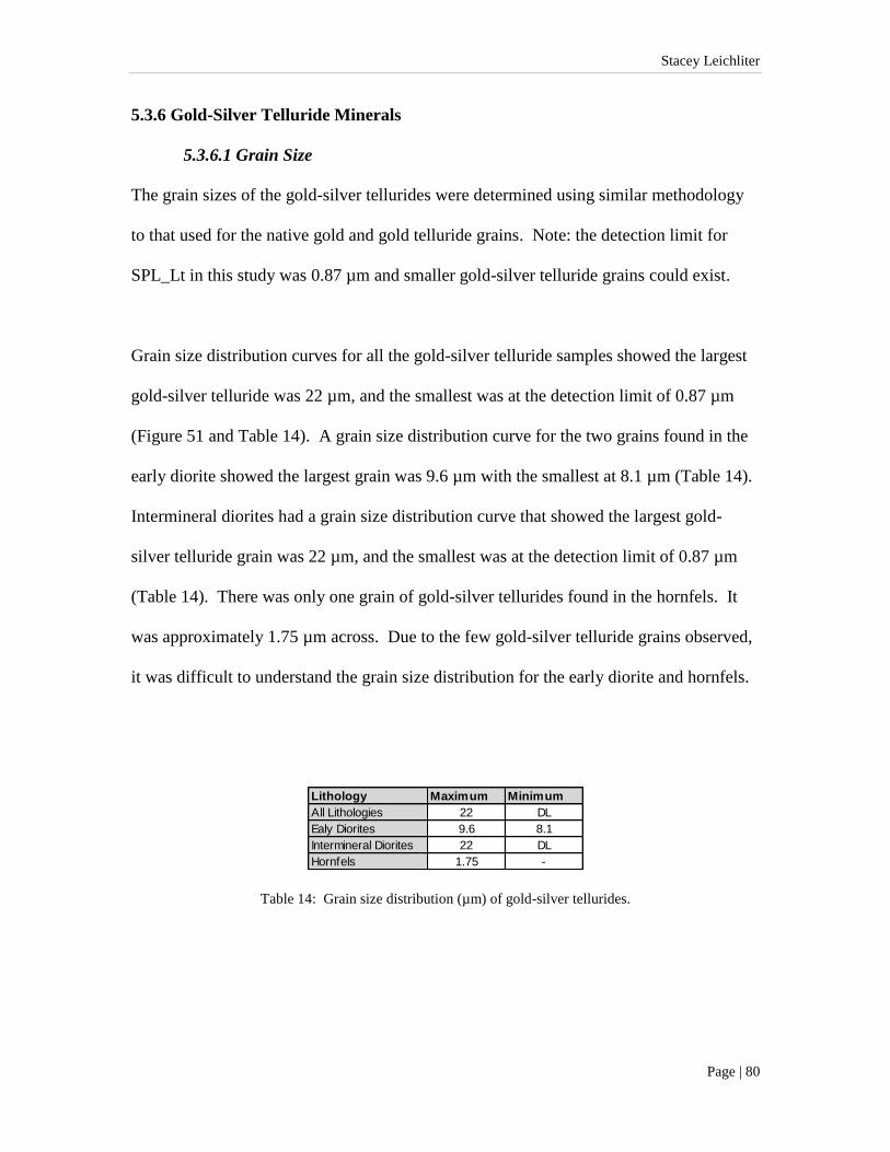
Stacey Leichliter

Page | 80

5.3.6 Gold-Silver Telluride Minerals

5.3.6.1 Grain Size

The grain sizes of the gold-silver tellurides were determined using similar methodology

to that used for the native gold and gold telluride grains. Note: the detection limit for

SPL_Lt in this study was 0.87 µm and smaller gold-silver telluride grains could exist.

Grain size distribution curves for all the gold-silver telluride samples showed the largest

gold-silver telluride was 22 µm, and the smallest was at the detection limit of 0.87 µm

(Figure 51 and Table 14). A grain size distribution curve for the two grains found in the

early diorite showed the largest grain was 9.6 µm with the smallest at 8.1 µm (Table 14).

Intermineral diorites had a grain size distribution curve that showed the largest gold-

silver telluride grain was 22 µm, and the smallest was at the detection limit of 0.87 µm

(Table 14). There was only one grain of gold-silver tellurides found in the hornfels. It

was approximately 1.75 µm across. Due to the few gold-silver telluride grains observed,

it was difficult to understand the grain size distribution for the early diorite and hornfels.


All Lithologies 22 DL

Ealy Diorites 9.6 8.1

Intermineral Diorites 22 DL

Hornfels 1.75 -

Table 14: Grain size distribution (µm) of gold-silver tellurides.

Stacey Leichliter

Page | 81

0

10

20

30

40

50

60

70

80

90

1005

3

45

38

32

27

22

19

16

13

.5

11

.4

9.6

8.1

6.8

5.7

4.8

4.1

3.4

2.9

2.4 2

1.7

5

1.4

5

1.2 1

0.8

7

0.7

3

Cu

mu

lati

ve P

assi

ng

(wt%

)

Sieve Size (µm)

AuAg Te Grain Size DistributionPh1 and Ph2 Samples

All Lithologies

Early Diorite


Hornfels

Figure 51: Grain size distribution of gold-silver tellurides (n = 63) in the Phase 1 and Phase 2 samples by

lithology: early diorite (n=2), intermineral diorite (n=60), and hornfels (n=1).

The PSSA average grain size of the gold-silver tellurides was calculated for all measured

grains to be approximately 2 µm. As mentioned before with the native gold and gold

telluride grains, the average PSSA grain size could possibly be overestimated due to

potential undetected, smaller grains. The intermineral diorites had a grain size of 2 µm.

The one measured grain of gold-silver tellurides located in the hornfels samples was 2

µm across (Table 8). Dominant mineral associations for the gold-silver tellurides were

with apatite, albite, and pyrite. The average grain size of the measured gold-silver

telluride grains associated with albite was 3 µm with the measured grains associated with

pyrite being 4 µm across (Table 9). The grain size of the measured gold-silver telluride

grains associated with the other gangue minerals (hornblende, actinolite, apatite, etc.) was

1 µm across.

Stacey Leichliter

Page | 82


Examples of mineral associations observed with the gold-silver tellurides are shown in

Figure 52. Gold-silver tellurides have an overall strong mineral association with apatite

followed by albite and pyrite (Figure 53 and Table 15).

.

Apatite

ThoriteAuAg Te

Amphibole

COL109_40-44 COL101_366-370

AuAg Te

Galena

K Feldspar

ab

Figure 52 a and b: Gold-silver telluride mineral associations observed in the Phase 1 and Phase 2 samples.

The find/small size of the gold-silver telluride grains and edge effect make it difficult to obtain high quality

images of these grains.

Figure 53: Summary of major mineral associations for gold-silver telluride mineralisation as in Table 15.

Stacey Leichliter

Page | 83

Lithology Gold (wt%) Albite (wt%) Apatite (wt%) Calcite (wt%) Epidote (wt%) K Feldspar (wt%) Pyrite (wt%) Thorite (wt%) Free Surface (wt%)

Early Diorite 0.00 50.00 0.00 0.00 0.00 0.00 0.00 0.00 0.00

Intermineral Diorite 0.10 11.24 13.18 9.18 8.49 5.65 30.99 11.88 6.11

Hornfels 0.00 0.00 100.00 0.00 0.00 0.00 0.00 0.00 0.00

All Lithologies 0.06 20.71 21.82 5.25 4.85 3.23 17.71 6.79 3.49

Table 15: Summary table of the major mineral associations for the gold-silver telluride mineralisation by

lithology.

5.3.6.3 Locking

Gold-silver telluride grains are dominantly locked within albite, pyrite, apatite, and K

feldspar (Figure 52 and Table 11). Albite contained the majority of the gold-silver

telluride grains (20.12%) followed by pyrite (17.48%) and apatite (15.79%).

5.3.7 Summary

Various minerals containing gold (native gold, gold tellurides, gold-silver tellurides) at

La Colosa had similar grain size distributions with roughly two populations, or bimodal,

(< 10 µm and > 10 µm) and average grain sizes (PSSA) from 2 µm to 4 µm (minimum =

1 µm and maximum = 37 µm). These average grain sizes were a function of the

detection limit of the grain measurements. The average could be smaller due to fine,

undetectable grains. The gold-silver tellurides were much smaller than the native gold

and gold tellurides. The larger native gold grains were associated with quartz with the

smaller ones associated with other sulfides. The larger populations (> 10 µm) of gold

telluride grains were associated with other sulfides and gangue minerals with the smaller

grains (< 10 µm) associated with pyrite. The larger distributions (> 10 µm) of gold-silver

tellurides grains were associated with pyrite, and smaller grains (< 10 µm) were

associated with other gangue.

Stacey Leichliter

Page | 84

The larger populations (> 10 µm) of gold grains tended to be associated with pyrite

and/or quartz. These two minerals occurred in both A and S type veins. The smaller

distributions (< 10 µm) of gold grains were observed with the feldspars (K feldspar,

albite, and/or plagioclase) these minerals tended to occur in the groundmass or matrix.

Native gold and gold tellurides were mainly associated with pyrite, and the gold-silver

tellurides were mostly associated with albite, apatite, and pyrite. There were more gold-

silver tellurides found with the intermineral diorites than the early diorites.

5.4 Vein Rich and Vein Poor Mineralisation

5.4.1 Introduction

To determine if there was a difference in the types of gold mineralisation, i.e. vein rich or

vein poor, a small number of samples (n=37) were analysed. The gold mineralisation in

the early diorites seemed to be in both veins and in groundmass with the sulfides. Gold

mineralisation in the intermineral diorites appeared to be mainly in the veins. Gold is

observed most common in the A and S veins that crosscut all the major lithologies (early

diorite, intermineral diorite, and hornfels). The differences in the modal mineralogy and

the gold deportment should help identify the traits of the different types of gold

mineralisation. There were 87 grains of gold mineralisation (native gold and gold

telluride) observed in the samples for this study (Table 16).

Stacey Leichliter

Page | 85

5.4.2 Methods

The MLA methods (XMOD and SPL_Lt) used to determine the gold deportment of the

vein rich and vein poor mineralisation were described in section 5.2. The logs and

photographs are in Appendices D and E (digital).

Sample ID From (m) To (m) Lithology Au g/t Au Grains AuTe Grains Classification

COL029_HG_01 190 190.1 EBX2 10.10 0 0 vein rich

COL029_HG_02 190.1 190.2 EBX2 10.10 12 4 vein rich

COL029_HG_03 190.2 190.3 EBX2 10.10 0 0 vein poor







COL029_HG_10 190.9 191 EBX2 1.45 0 0 vein rich

COL029_HG_11 191 191.1 EBX2 4.33 0 0 vein poor








COL049_HG_01 252 252.1 IBX 0.20 0 0 vein rich

COL049_HG_02 252.1 252.2 IBX 0.17 0 0 vein rich

COL049_HG_03 252.2 252.3 IBX 0.19 0 0 vein poor







COL049_HG_10 252.9 253 IBX 3.70 0 0 vein rich

COL049_HG_11 253 253.1 IBX 0.19 0 0 vein rich









Avg Au Grade 2.68

Total Grains 51 36

Table 16: Summary table of the gold grains found in the vein rich versus vein poor samples.

Stacey Leichliter

Page | 86

5.4.3 Vein Rich Mineralisation

The modal mineralogy of the ten cm interval samples that were determined to be vein

rich by logging had an abundance of plagioclase, K feldspar, albite, and quartz. When

compared with the QXRD data of the less veined samples of the early and intermineral

diorite lithologies (Table 7), the data showed an enrichment of K feldspar, Ca amphibole,

and pyrite. It also showed a depletion of plagioclase, quartz, and actinolite (Table 17).

Plagioclase is a dominant mineral found in the “fresh” or less altered rocks and K

feldspar is a major mineral found in the potassic alteration assemblage. Pyrite is found in

the veins (A, B, D, and S type veins). The enrichments and depletions are consistent with

the alteration and vein types associated with the gold mineralisation.

Mineral Vein Rich (wt %) Vein Poor (wt %)

Actinolite 0.43 0.07

Albite 8.31 11.78

Apatite 0.59 0.44

Biotite 4.45 7.16

Ca_Amphibole 5.54 0.37

Chalcopyrite 0.03 0.13

Chlorite_Mg 2.21 0.95

ChloriteFe 0.72 0.14

Epidote 0.15 0.52

K feldspar 17.32 9.67

Hornblende 3.35 0.76

Phlogopite 1.31 2.96

Plagioclase 40.78 51.73

Pyrite 6.41 4.65

Pyrrhotite 0.26 0.17

Quartz 7.24 7.57

Rutile 0.11 0.22

Siderite 0.01 0.17

Talc 0.05 0.37

Titanite 0.53 0.13

Total 100.00 100.00

Table 17: Modal mineralogy of vein rich and vein poor mineralisation samples.

Stacey Leichliter

Page | 87

There were 31 gold grains observed in the vein rich samples. The gold grains consisted

of native gold (22) and gold tellurides (9). They were observed in both the early and

intermineral diorites. The grain size distribution curve for the vein rich gold grains

showed the gold tellurides (average 2 µm) were smaller than the native gold grains

(average 16 µm) (Figure 54 and Table 18).

0.00

10.00

20.00

30.00

40.00

50.00

60.00

70.00

80.00

90.00

100.00

32

27

22

19

16

13

.5

11

.4

9.6

8.1

6.8

5.7

4.8

4.1

3.4

2.9

2.4 2

1.7

5

1.4

5

1.2 1

0.8

7

0.7

3

Cu

mu

lati

ve P

assi

ng

(wt%

)

Sieve Size (µm)

Grain Size DistributionVein Rich vs. Vein Poor Samples

VR Au Avg

VR AuTe Avg

VP Au Avg

VP AuTe Avg

Figure 54: Grain size distribution curves for the native gold and gold telluride grains in the vein rich (VR)

and vein poor (VP) samples.

Mineral 029_HG-02 029_HG_16 029_HG_17 049_HG_08 049_HG_19 Avg PSSA Avg Grain Size

Gold 0.42 0.88 0.40 0.00 0.31 0.40 11.77

Au_telluride 0.31 0.00 2.74 4.35 7.23 2.93 1.61

Table 18: PSSA (µm) of the gold mineralisation in the vein rich samples.

Stacey Leichliter

Page | 88

Minerals associated with the native gold in the samples dominated by veins were quartz,

and pyrite (Figure 55). The gold telluride grains analysed in the vein rich samples

showed mineral associations of quartz and native gold (Table 19).

Figure 55: Major mineral associations for the mineralisation in the vein rich vs. vein poor samples.

Mineral Gold (wt%) Albite (wt%) Biotite (wt%) Chalcopyrite (wt%) Chlorite_Mg (wt%) K Feldspar (wt%) Phlogopite (wt%) Plagioclase (wt%) Pyrite (wt%) Quartz (wt%) Au_telluride (wt%)

Gold - Vein rich 0.00 2.51 6.68 0.00 0.00 8.47 3.28 26.36 11.46 12.12 0.25

Gold - Vein poor 0.00 11.82 1.77 1.19 1.88 8.33 0.00 21.52 3.67 2.15 0.49

Gold Telluride - Vein rich 12.26 0.00 0.00 0.00 0.00 4.14 0.00 0.00 0.00 44.06 0.00

Gold Telluride - Vein poor 0.89 13.22 0.00 0.00 4.59 3.61 0.00 21.63 0.00 1.29 0.00

Table 19: Major minerals associated with gold mineralisation in the vein rich and vein poor sample.

5.4.4 Vein Poor Samples

There were 56 gold grains observed in the vein poor samples (29 native gold and 27 gold

tellurides). The vein poor samples were all from the early diorites. The modal

mineralogy of these samples had an abundance of plagioclase, albite, K feldspar, quartz,

and biotite. When compared with the QXRD data from the weakly altered early diorite

Stacey Leichliter

Page | 89

samples (Table 7), it suggested an enrichment of biotite and depletion of K feldspar,

quartz, and pyrite in the mineralised disseminated samples (Table 17). The enrichment of

biotite suggested secondary biotisation of the pyrite, which indicated potassic alteration.

Grain size distribution curves for gold grains in the vein poor samples showed similar

grain sizes between the native gold and gold tellurides (Figure 54). The average grain

size (PSSA method) of the vein poor samples was determined to be 9 µm for native gold

and 9 µm for gold tellurides (Table 20).

Mineral 029_HG_06 029_HG_12 Avg PSSA Avg Grain Size

Gold 0.62 0.39 0.50 9.37

Au_telluride 0.52 0.49 0.50 9.33

Table 20: PSSA (µm) of the gold mineralisation of the vein poor samples.

Mineral associations for the native gold grains in the samples with fewer number of veins

were chalcopyrite and gold telluride (Figure 55). The gold telluride grains had mineral

associations of gold and chlorite (Table 19).

5.4.5 Summary

Native gold and gold telluride mineralisation was observed in both the vein rich and vein

poor samples. Vein poor samples showed enrichments of biotite, while the vein rich

samples showed enrichments of K feldspar, Ca amphibole, and pyrite, which are two

different characteristics of potassic alteration. The average grain size of the native gold

grains observed in the vein rich samples was coarser than the vein poor samples. The

vein poor samples had a more consistent average grain size between the native gold and

Stacey Leichliter

Page | 90

the gold telluride mineralisation. The major minerals associated with the gold

mineralisation in the samples with vein rich samples were pyrite and quartz. These

minerals, especially quartz, were mainly found in the veins. Major minerals associated

with the gold mineralisation in the vein poor samples were chalcopyrite and chlorite.

These minerals were commonly found in either veins or the groundmass.

5.5 Summary of Gold Mineralisation

Detailed logging performed in this study of the Phase 1 and Phase 2 samples (Appendix

D), along with other diamond drill core, indicated that gold mineralisation was associated

with potassic alteration. Pervasive potassic alteration was observed with K feldspar

forming in the groundmass, and quartz depleted. This was evident in the XMOD and

QXRD data with the quartz becoming depleted as the alteration became stronger. The

strongest potassic alteration showed replacement of the original groundmass by K

feldspar and lesser amounts of biotite. Feldspar phenocrysts were also altered with the

irregular boundaries forming as part of K feldspar replacement.

The alteration assemblage in high gold mineralisation was potassic or potassic-calcic in

composition. Vein types common in the gold mineralisation were the sulfide veins (S) in

the west and quartz-sulfide veins (A) in the eastern section of the deposit (Figure 43). A

particular vein type responsible for all the gold mineralisation has not been observed.

The telluride related mineralisation was concentrated in the western section of the

deposit, and the strong disseminated sulfide mineralisation was located in the eastern side

(Figure 44). Assuming the samples analysed in the QXRD and XMOD testwork were

Stacey Leichliter

Page | 91

representative of the deposit, the results from the QXRD and XMOD analyses showed

overall mineral enrichments were typical minerals from the potassic-calcic alteration

assemblages (e.g. K feldspar, biotite, amphibole, biotite, and pyrite) and the depletions

were minerals typical in the original rock (e.g. plagioclase and quartz). It appeared

potassic-calcic alteration was the dominant alteration within the mineralised samples and

in the strongly altered rocks. The diorite samples were enriched in amphibole and the

hornfels samples were enriched in biotite, and both major minerals of enrichment were

characteristic of potassic and potassic-calcic alteration.

Gold grains analysed in the early diorites were very fine-grained with native gold and

gold tellurides about 4 µm to 5 µm and gold-silver tellurides about 10 µm across and

were associated predominantly with pyrite, which is associated with potassic or potassic-

calcic alteration. The intermineral diorite mineralisation was very fine-grained (gold

grains < 10 µm), with native gold and gold tellurides about 5 µm across and finer gold-

silver tellurides at 2 µm, and a dominant pyrite association. Minerals associated with the

gold mineralisation in the intermineral diorites were typical of potassic or potassic-calcic

alteration. Gold grains observed in the hornfels were finer grain sizes with native gold,

gold tellurides, and gold-silver tellurides at 1 µm to 2 µm. The gold grains in hornfels

had a major association with pyrite, which is typical of potassic or potassic-calcic

alteration in the presented porphyry gold deposit models (Sillitoe, 2000 and Sillitoe,

2010).

Stacey Leichliter

Page | 92

There seemed to be a difference in the gold mineralisation in the samples with vein rich

samples and those mainly vein poor. The samples with vein-dominant gold

mineralisation had a higher amount of K feldspar, Ca amphibole, and pyrite. The

samples with few veins had more biotite. The quartz contents were similar in both

sample sets. Native gold was coarser in the vein rich samples. Gold-telluride

mineralisation was similar in the vein poor samples. There were no gold-silver tellurides

observed in any of the vein rich or vein poor samples. Quartz and pyrite were associated

with the gold mineralisation in the vein rich samples. Chalcopyrite and chlorite were

associated with the gold in the vein poor samples. The gold mineralisation in the vein

rich samples appeared to be associated with potassic or potassic-calcic alteration (Table

19) as typical in gold porphyry deposits (Sillitoe, 2000 and Sillitoe, 2010).

Stacey Leichliter

Page | 93

Chapter 6: Predictive Geometallurgical

Gold Recovery Model

6.1 Introduction

The recovery process has not yet been determined for the La Colosa deposit, and there

has not been any published work to date on its gold deportment, geometallurgy, and

recovery. Metallurgical testwork is currently underway. There have been preliminary

analyses, such as cyanide leach testwork (shake leach assays and bottle rolls), gravity

concentration, and flotation concentration performed. These processes are described in

section 6.2. Data from these tests will be used in the following section where applicable.

This section of the study aims to construct an initial predictive geometallurgical recovery

model for the gold mineralisation at La Colosa. Geometallurgical recovery models can

use mineralogy and deportment information along with analytical data from recovery

testwork to predict how gold recovery is likely to vary with changes in the response to the

extraction and processing of the ore (i.e. blasting, comminution, cyanidation, or

flotation). Measured gold recovery is a function of total measured gold (fire or head

assay) to measured extractable gold (cyanidation, flotation, or gravity assays). Recovery

is a function of many parameters such as texture, grain size, liberation, reagents,

processes, crushing, and grinding. Details are provided in the following sections.

Stacey Leichliter

Page | 93

Chapter 6: Predictive Geometallurgical

Gold Recovery Model

6.1 Introduction

The recovery process has not yet been determined for the La Colosa deposit, and there

has not been any published work to date on its gold deportment, geometallurgy, and

recovery. Metallurgical testwork is currently underway. There have been preliminary

analyses, such as cyanide leach testwork (shake leach assays and bottle rolls), gravity

concentration, and flotation concentration performed. These processes are described in

section 6.2. Data from these tests will be used in the following section where applicable.

This section of the study aims to construct an initial predictive geometallurgical recovery

model for the gold mineralisation at La Colosa. Geometallurgical recovery models can

use mineralogy and deportment information along with analytical data from recovery

testwork to predict how gold recovery is likely to vary with changes in the response to the

extraction and processing of the ore (i.e. blasting, comminution, cyanidation, or

flotation). Measured gold recovery is a function of total measured gold (fire or head

assay) to measured extractable gold (cyanidation, flotation, or gravity assays). Recovery

is a function of many parameters such as texture, grain size, liberation, reagents,

processes, crushing, and grinding. Details are provided in the following sections.

Stacey Leichliter

Page | 94

6.2 Gold Recovery Processes

There are many different processes to extract gold (e.g. gravity concentration, flotation

concentration, leaching, and roasting (Marsden and House, 2006). The processes being

considered for the La Colosa porphyry deposit are gravity concentration, flotation

concentration, and cyanide leaching. Each process is tailored to the overall mineralogy

associated with the gold mineralisation. Gravity and flotation concentration allow for the

pre-concentration of the gold before the feed undergoes cyanide leaching. Gravity

concentration is used to recover the free gold at coarser grain sizes (Marsden and House,

2006 and Wills and Napier-Mann, 2006). Flotation concentration is used to recover free

gold and gold associated with sulfides or other floatable minerals (Wills and Napier-

Munn, 2006). Cyanide leaching, such as heap leaching, allows for the extraction of the

gold from the rock when ore is associated with gangue minerals, such as feldspars and

quartz (Marsden and House, 2006). Each of these methods has been tested for future

application for the processing of gold ore at La Colosa.

6.2.1 Gravity Concentration

The gravity concentration method can be used to recover the free gold and gold that is

associated with heavy or dense minerals (e.g. sulfides, barite, and other dense minerals);

(Marsden and House, 2006) through a process which separates the particles by specific

gravity, either by fluid, by gravity, or centrifugal force (Fuerstenau and Han, 2003).

Their movement is not only dependent on the specific gravity of the mineral but also on

its size and shape, with larger grains influenced more than smaller ones (Wills and

Napier-Munn, 2006). The minimum grain size of the gold must be at least 50 µm (Wills

Stacey Leichliter

Page | 95

and Napier-Munn, 2006) with some gold grains as small as 10 µm (Marsden and House,

2006) for the process to work efficiently.

The basic theory behind gravity concentration is that minerals of different specific

gravities separate by their response to gravity during processing, with heavier particles

separating from the lighter one. There are many different types of devices used to

concentrate the ore by gravity. The most common are the gravity separators, jigs,

pinched sluices and cones, spirals, centrifugal concentrators, and shaking tables (Wills

and Napier-Munn, 2006). The gravity concentration methods are simple, less costly than

flotation, and produce little pollution (Wills and Napier-Munn, 2006).

6.2.2 Flotation Concentration

Flotation is an efficient processing method for the recovery of free gold and gold

associated with sulfides, provided the gold ore is fully liberated (Wills and Napier-Munn,

2006). The ability to separate the minerals by flotation is determined by the differences

in the wettability of the minerals. Minerals, such as sulfides, can float because they are

naturally hydrophobic, or water-repellent (Fuerstenau and Han, 2003). Flotation works

well for particles between 20 µm and 200 µm, although finer sizes may be floated with

more chemical controls to limit the gangue interference (Marsden and House, 2006).

Gold tellurides may also be efficiently recovered by flotation (Marsden and House,

2006). There can be multiple stages and cells in the flotation process called flotation

circuits, which can have rougher-scavenger-cleaner components. Feed enters the first

cells in the circuit and then is transferred from cell to cell, with the pulp levels raised

Stacey Leichliter

Page | 96

further down the circuit due to less floatable particles. The rougher concentrate is formed

from the initial concentrate. The cleaner is the stage where the pulp content is kept low

to produce a clean, high-grade concentrate (Fuerstenau and Han, 2003) and the scavenger

stage is where the remaining flotable gold is collected (Marsden and House, 2006).

6.2.3 Cyanide (NaCN) Leaching

Leaching is the extraction of a metal by dissolving it into solution (Marsden and House,

2006). This process requires both a complexant and an oxidant to control the reaction at

desired rates (Marsden and House, 2006). Cyanide is the preferred reagent to use for

precious metals because it is inexpensive and is reactive with gold and silver. Oxygen

(either free or pumped) is typically the oxidant used with cyanide leaching. Options

other than cyanide do exist (chloride, thiourea, and thio sulfate); however thse have the

disadvantages of being corrosive, carcinogenic, and expensive. They are used by some

sites because they have advantages of being environmentally safer than cyanide (Marsden

and House, 2006). There are different methods for gold cyanidation leaching: agitation,

heap, intensive cyanidation, vat, and in situ (Fuerstenau and Han, 2003 and Marsden and

House, 2006).

After the gold is in solution, i.e. has been leached from the ore, it needs to be

concentrated from the dilute solution. This is done by using activated carbon or a

synthetic ion exchange resin for adsorbing the gold solution in methods such as carbon-

in-pulp (CIP) or carbon-in-leach (CIL) (Fuerstenau and Han, 2003 and Marsden and

House, 2006). Gold is separated from the carbon and concentrated into a solid form by

Stacey Leichliter

Page | 97

electrowinning or zinc precipitation (Marsden and House, 2006). Cyanide leaching is

preferred in deposits with gold associated with gangue minerals such as feldspars, quartz,

and biotite, because these minerals have little to no interference with the gold dissolution

(Marsden and House, 2006). Gold associated with tellurides or sulfides (iron, copper, or

lead) does not leach efficiently, because these minerals affect the gold dissolution rate

due to encapsulation of the gold (Marsden and House, 2006). The cyanide leach

applications which were used in this project were the shake leach test, a short intense

cyanide leach, and bottle rolls. All of these tests were performed in commercial

laboratories, and the cyanide leach analyses had all the variables (e.g. cyanide

concentration, oxygen, pH, and leach time) held constant. Information on the shake leach

assay and bottle roll testwork is found in Appendices A and B.

Cyanidation is being considered for La Colosa with the preferred extraction process being

either CIP or CIL. Gravity is also being considered due to the concentration of coarse

gold along the major structure in the central part of the deposit. Other reagents and

processes have been ruled out due to their expense and effect on recovery.

6.3 Geometallurgical Gold Recovery Modelling

6.3.1 Geometallurgical Modelling

In order to build a predictive geometallurgical recovery model, the recovery data needs to

be linked or compared with the geology and other traits (gold grade, hardness, and

recovery) that represent the samples. Geometallurgical modelling uses geological

information, such as drill logs, assay testwork, and optical microscope work, along with

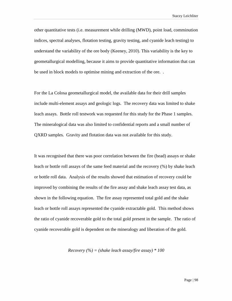
Stacey Leichliter

Page | 98

other quantitative tests (i.e. measurement while drilling (MWD), point load, comminution

indices, spectral analyses, flotation testing, gravity testing, and cyanide leach testing) to

understand the variability of the ore body (Keeney, 2010). This variability is the key to

geometallurgical modelling, because it aims to provide quantitative information that can

be used in block models to optimise mining and extraction of the ore. .

For the La Colosa geometallurgical model, the available data for their drill samples

include multi-element assays and geologic logs. The recovery data was limited to shake

leach assays. Bottle roll testwork was requested for this study for the Phase 1 samples.

The mineralogical data was also limited to confidential reports and a small number of

QXRD samples. Gravity and flotation data was not available for this study.

It was recognised that there was poor correlation between the fire (head) assays or shake

leach or bottle roll assays of the same feed material and the recovery (%) by shake leach

or bottle roll data. Analysis of the results showed that estimation of recovery could be

improved by combining the results of the fire assay and shake leach assay test data, as

shown in the following equation. The fire assay represented total gold and the shake

leach or bottle roll assays represented the cyanide extractable gold. This method shows

the ratio of cyanide recoverable gold to the total gold present in the sample. The ratio of

cyanide recoverable gold is dependent on the mineralogy and liberation of the gold.

Recovery (%) = (shake leach assay/fire assay) * 100

Stacey Leichliter

Page | 99

Since more than one factor may be responsible for causing variability in traits (e.g. grade,

hardness, grindability, and recovery) univariate statistics may not be able to fully describe

the data. The use of multivariate statistics is better suited for this purpose (Davis, 2002).

The multivariate statistical analyses used to develop the geometallurgical model included

correlation analysis, Mahalanobis Distance analysis, Principal Components Analysis

(PCA), and multiple regression analysis (e.g. Davis, 2002 and Keeney, 2010) Correlation

analysis allows for the identification of correlating or related parameters (Davis, 2002).

Mahalanobis Distance analysis allows for the classification of anomalous data or outliers

(Davis, 2002 and ioGAS, 2011). For more information, see Appendix H. PCA takes

multiple variables in several dimensions in space and transforms them into two

dimensional space, so they may be viewed (Davis, 2002 and ioGAS, 2011). See

Appendix I for more information on the PCA. Multiple regression analysis is used to

derive equations to predict one parameter, using other related parameters (Davis, 2002).

To construct a predictive geometallurgical recovery model for the La Colosa porphyry

gold deposit, the relationships between recovery test data and multi-element assay,

modal mineralogy, and calculated mineralogy, were analysed using different statistical

methods, Mahalanobis Distance analysis and PCA. The recovery data to use for

modelling was limited to cyanide leach data (shake leach assays and bottle roll assays),

because gravity and flotation testwork had not been completed at the time of the project.

Details of the theory and background behind some of the statistical calculations and

methods can be found in Appendices H and I.

Stacey Leichliter

Page | 100

The computer software utilised for the majority of the statistical analyses and modelling

was ioGAS. This was due to its ease of visualising and classifying data, as well as

complex multivariate statistical analyses. The program allows for easy export of the

classified and estimated values which can be then wireframed in other software, such as

Leapfrog. The ioGAS methodologies are found following the statistical theories in

Appendices H and I.

6.3.2 Methods for Gold Recovery Modelling

The methodology used to create the geometallurgical gold recovery estimate model

included using various statistical techniques to analyse for outliers, identify and classify

traits, and domain the dataset. The methodology to develop these geometallurgical

recovery models used techniques described in Davis (2002) and Keeney (2010). These

steps include the following:

1. Identify anomalies in the recovery data using Mahalanobis Distance.

2. Perform Correlation Analysis to identify correlations between gold

(head or fire) assay and other elements or minerals (i.e. tellurium, sodium, sulfur,

and copper). This is done by starting with the entire element dataset and then

selecting the elements with the strongest correlations. These elements will be

used as inputs into the PCA.

3. Perform a Principal Components Analysis (PCA), using the elements selected as

inputs in step 2, to identify variability. A scatter plot is constructed using the two

selected principal components which contain the highest variability.

4. Using the scatter plot, define classes based on similar groupings of elements or

Stacey Leichliter

Page | 101

minerals and create a discriminant diagram of the classes. Perform linear and non-

linear regressions using the classes of the discriminant diagram and elements

strongly correlated with the recovery data to model the recoverable gold.

5. Create process performance domains of the data and wireframe to check.

6. Evaluate the model and re-iterate the modelling steps as additional data is

obtained.

7. Incorporate the estimated data into the resource or geologic block model.

Two recovery estimate models were constructed to estimate gold recovery at La Colosa :

to estimate recovery by cyanide recovery using shake leach testing and to estimate

recovery by cyanide leaching using bottle roll testing. (Appendix G).

6.3.3 Model 1: To Estimate Gold Recovery as Measured by Shake Leach Tests

The first recovery model for La Colosa was built using the shake leach assay data and

multi-element assay data provided by the site (Appendix G). Shake leach analyses were

carried out by an outside laboratory and represented the extractable gold. This data

included 964 samples from diamond drill holes COL001, COL004, COL006, COL009,

COL012, COL014, and COL015. The samples with gold grades from fire (head) assay

which were lower than the cut off grade of 300 ppb or 0.3 g/t were filtered out along with

any samples that had a measured recovery greater than 100%. The remaining samples

totalled approximately 650 and represented most major lithologies (i.e. early diorite,

intermineral diorite, and hornfels) which contain the majority of the gold mineralisation.

Multi-element assay data for the drill core from the same sample intervals as the shake

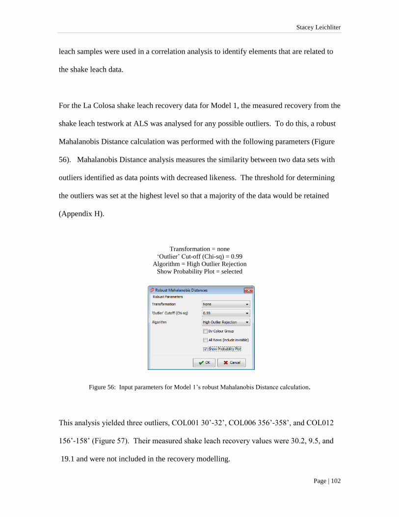
Stacey Leichliter

Page | 102

leach samples were used in a correlation analysis to identify elements that are related to

the shake leach data.

For the La Colosa shake leach recovery data for Model 1, the measured recovery from the

shake leach testwork at ALS was analysed for any possible outliers. To do this, a robust

Mahalanobis Distance calculation was performed with the following parameters (Figure

56). Mahalanobis Distance analysis measures the similarity between two data sets with

outliers identified as data points with decreased likeness. The threshold for determining

the outliers was set at the highest level so that a majority of the data would be retained

(Appendix H).

Transformation = none ‘Outlier’ Cut-off (Chi-sq) = 0.99

Algorithm = High Outlier Rejection

Show Probability Plot = selected

Figure 56: Input parameters for Model 1’s robust Mahalanobis Distance calculation.

This analysis yielded three outliers, COL001 30’-32’, COL006 356’-358’, and COL012

156’-158’ (Figure 57). Their measured shake leach recovery values were 30.2, 9.5, and

19.1 and were not included in the recovery modelling.

Stacey Leichliter

Page | 103

Input variables to the model were selected based on a correlation analysis with the gold

fire (head) assay (Table 21). Stronger correlations are closer to 1 and weaker correlations

are equal to 0. The positive values in the correlation calculations (Table 21) indicate a

direct relationship between the elements, and negative values suggest an inverse

Figure 57: Distribution curve for the Mahalanobis Distance (M-dist) for the measured recovery data from

ALS.

relationship. The stronger the relationship, the closer the absolute value is to 1. There

were no distinctly strong correlations with the gold assay, but weaker correlations existed

with elements such as potassium, tellurium, and calcium.

Robust Correlation AUPPM CAPPM KPPM TEPPM

AUPPM 1.00 -0.40 0.35 0.23

CAPPM -0.40 1.00 -0.82 0.23

KPPM 0.35 -0.82 1.00 -0.33

TEPPM 0.23 0.23 -0.33 1.00

Table 21: Robust correlation for Model 1 Principal Components Analysis.

Stacey Leichliter

Page | 104

A Principal Components Analysis was performed on the head (fire) assay results (647

samples) to look for the elements that were strongly compared with the fire assay for

gold. These elements were calcium, potassium, and tellurium. These variables (Au, Ca,

K, and Te) were used in the Principal Components Analysis. The input parameters for

the calculation are listed (Figure 58):

Transformation = Box Cox Trim 5% (power)

Use Correlation Matrix = selected


Number of Principal Components = 4

Show Report = selected

Figure 58: Input parameters for the robust Principal Components Analysis (PCA).

PCA was carried out on the sample data set using the following parameters: gold assay

(fire or head) and it’s strongly correlated elements. This was done in order to spread out

the data and to identify clusters while maintaining data variance (Davis, 2002 and

Keeney, 2010). The amount of variability in the data set accounted for by each

component decreases with increasing component number, i.e. the first principal

component accounts for the highest degree of variability and the last component accounts

for the least amount of variability (Appendix I). A transformation (logarithmic or power

– box cox) of the assay data was necessary, because it was not normally distributed. The

Stacey Leichliter

Page | 105

results from the robust Principal Components Analysis with Au, Ca, K, and Te are shown

in the following tables and figures.

Eigenvectors PC1 PC2 PC3 PC4

AUPPM -0.37 -0.64 0.68 0.00

CAPPM 0.63 0.01 0.36 -0.69

KPPM -0.64 0.09 -0.26 -0.72

TEPPM 0.24 -0.76 -0.59 -0.10

Table 22: Eigenvectors for Model 1 Principal Components Analysis.

The eigenvector results can indicate the contribution of the variable to the overall dataset

(Table 22). If it is close to zero, it does not have much of an important role in the PCA.

The positive and negative values are the direction of each variable. The PCA report also

provided plots of the principal components in two dimensions, e.g. PC1 versus PC2, PC1

versus PC3, etc. (Figures 59- 64).

Figure 59: Plot of PC1 versus PC2.

Stacey Leichliter

Page | 106




Stacey Leichliter

Page | 107



The decision to determine which principal components (PC1, PC2, etc.) to use for the

classifications depends on the amount of data variance accounted for (higher the better)

and the spread of the eigenvectors. Eigenvectors are a set of coordinates in multiple

dimensions in space that define the direction of a semiaxis or hyperellispsoid of the data

set (Davis, 2002). The eigenvalues represent the stretch or length of the semiaxis of the

ellipsoid (Davis, 2002).

Stacey Leichliter

Page | 108

The resultant principal components were analysed for the greatest variance and spread.

Notice the first two plots (Figures 59 and 60) have the greatest spread of the variables,

with the second, PC1 versus PC3 having the largest (Figure 60). This spread of the

variables allowed for clustering of the data with similar multivariate characteristics. The

principal components (PC1 and PC3) were used in plotting the data in a multivariate

scatter plot, because these two principal components had the greatest amount of spread

between the eigenvectors for each element (variance = 65%). Data from the PC1 versus

PC3 plot was displayed in a scatter plot (Figure 65).

Samples in that multivariate scatter plot were classified based on trends or groupings of

the samples (i.e. potassium, tellurium, and/or calcium content, and average mineralogy),

and a polygon was drawn around the zones with common traits (Figure 66). Average

mineralogy was a term used to classify the remainder of the samples that tended to plot in

the average zones of the scatter plots. The result of the classification process was the

discriminant diagram (Figure 67). The samples were distributed among the different

classes (High Calcium = 196, High Potassium = 131, Low Tellurium = 149, and Average

Mineralogy = 174). PCA calculations in this thesis used ioGAS software (ioGAS, 2011).

Stacey Leichliter

Page | 109

Figure 65: Multivariate scatter plot of PC1 and PC3 coloured by major rock type.

Figure 66: Scatter plots of different variables to determine the clusters of the data set.

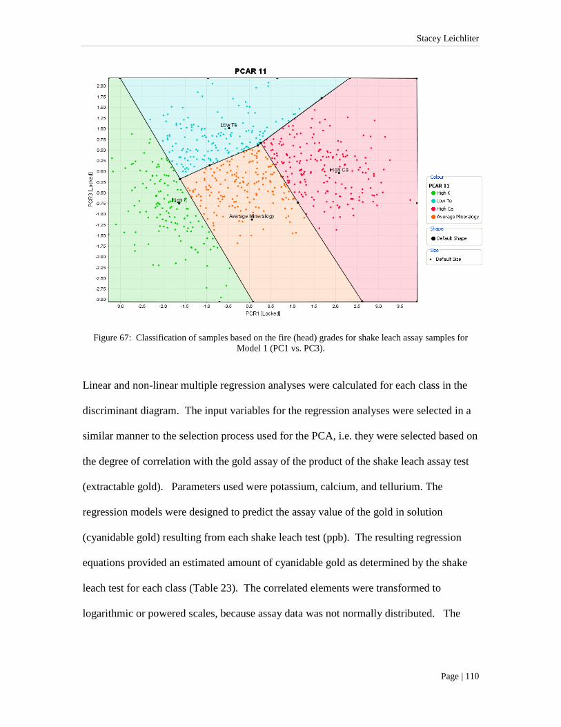
Stacey Leichliter

Page | 110

Figure 67: Classification of samples based on the fire (head) grades for shake leach assay samples for

Model 1 (PC1 vs. PC3).

Linear and non-linear multiple regression analyses were calculated for each class in the

discriminant diagram. The input variables for the regression analyses were selected in a

similar manner to the selection process used for the PCA, i.e. they were selected based on

the degree of correlation with the gold assay of the product of the shake leach assay test

(extractable gold). Parameters used were potassium, calcium, and tellurium. The

regression models were designed to predict the assay value of the gold in solution

(cyanidable gold) resulting from each shake leach test (ppb). The resulting regression

equations provided an estimated amount of cyanidable gold as determined by the shake

leach test for each class (Table 23). The correlated elements were transformed to

logarithmic or powered scales, because assay data was not normally distributed. The

Stacey Leichliter

Page | 111

strength of fit or coefficient of determination, R2, describes the confidence or strength of

the equation with strong being close to 1 and weak is equal to 0 (Davis, 2002).

Regression Equations for Model 1

Class Regression Equation for Gold Concentration # Samples R2 Average Relative Error (%)

High Calcium AU15_PPB_SL = 10 ̂((0.9368 * LOG(AUPPM)) + (0.0579 * LOG(BIPPM)) + (-0.05001 * LOG(TEPPM)) + 2.8826) 196 0.97 11.36

High Potassium AU15_PPB_SL= 10^((0.9276 * LOG(AUPPM)) + (0.04216 * LOG(TEPPM)) + 2.8872) 131 0.97 13.16

Low Tellurium AU15_PPB_SL = 10 ̂((0.9236 * LOG(AUPPM)) + (0.02651 * LOG(BIPPM)) + (0.07558 * LOG(NAPPM)) + (-0.04322 * LOG(TEPPM)) + 2.5292) 149 0.97 11.36

Average Mineralogy AU15_PPB_SL = 10 ̂((0.902 * LOG(AUPPM)) + (0.05023 * LOG(BIPPM)) + (-0.01756 * LOG(MOPPM)) + (-0.01691 * LOG(TEPPM)) + 2.9027) 174 0.97 9.29

Table 23: Table of regression equations used to estimate gold recovery in Model 1.

To determine the average relative error of the resultant model to estimate the gold

recovery by shake leach, the regression equations calculated for each class were then

applied to the measured shake leach recovery sample data set (n = 650). The measured

data set was divided into classes using the discriminant diagram designed for the model,

and then the regression equations for each developed class were applied in order to

calculate the estimated gold assay value of material produced by the shake leach test.

Next, estimated recovery by shake leach was determined by dividing the estimated shake

leach assay by the fire (head) gold assay and multiplying by 100 for the percentage.

Finally, the average relative error was calculated for the entire shake leach estimated

recovery model data set and for each class.

Avg Relative Error =100* (Absolute value (fire assay – est shake leach gold assay))

(fire assay)

Error in the measured gold fire assay was reported from the ALS laboratory to be 7%

(ALS written communication, 2012). Shake leach tests have a reported error of

approximately 7.5% (ALS written communication, 2012). This gave an overall error of

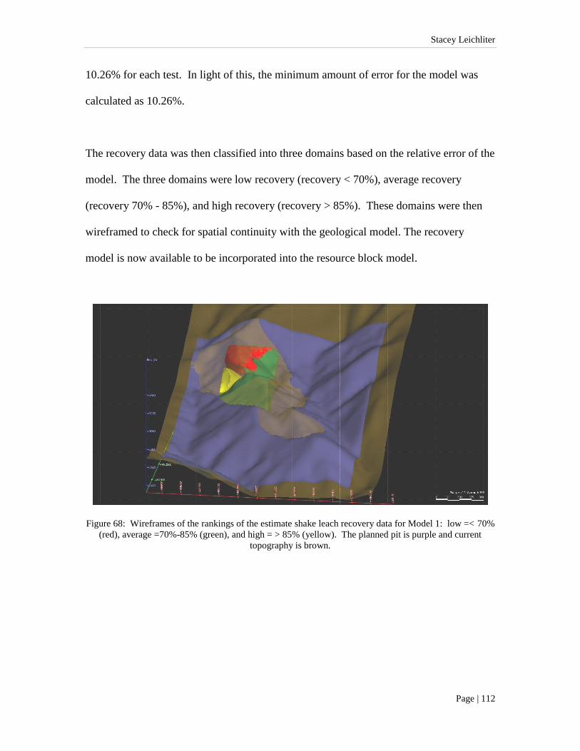
Stacey Leichliter

Page | 112

10.26% for each test. In light of this, the minimum amount of error for the model was

calculated as 10.26%.

The recovery data was then classified into three domains based on the relative error of the

model. The three domains were low recovery (recovery < 70%), average recovery

(recovery 70% - 85%), and high recovery (recovery > 85%). These domains were then

wireframed to check for spatial continuity with the geological model. The recovery

model is now available to be incorporated into the resource block model.

Figure 68: Wireframes of the rankings of the estimate shake leach recovery data for Model 1: low =< 70%

(red), average =70%-85% (green), and high = > 85% (yellow). The planned pit is purple and current

topography is brown.

Stacey Leichliter

Page | 113

Figure 69: Entire drill hole database (September 2011) assay samples as they plot on the discriminant

diagram as shown in Figure 67.

Using the classification diagram (Figure 67), the shake leach recovery for the entire drill

hole database for September 2011 (filtered to only samples containing gold grades greater

than 0.3 ppm or 0.3 g/t) (n=14,376) was then estimated using the recovery model shown

in Figure 69. Based on the initial discriminant diagram, the samples were divided into

the same classes as done in the prior model for the smaller sample set (Figure 70).

Stacey Leichliter

Page | 114

Figure 70: September 2011 drill hole assay data classified using the discriminant diagram.

Gold recoveries for the drill hole data were then estimated using the same regression

equations established for the classes from the diagram (Table 23). The recovery data was

domained and then wireframed to check the spatial continuity throughout the deposit

(Figure 71).

Figure 71: Wireframes of the estimated shake leach recovery domains (Low = < 70% (red), average =

70%-85% (green), and high >85% (yellow) to show spatial continuity. The planned pit is purple and

current topography is brown.

Stacey Leichliter

Page | 115

6.3.4 Model 2: To Estimate Gold Recovery Measure by Bottle Roll Tests

The second recovery model was designed to predict recovery as determined by bottle roll

tests from the Phase 1 samples. Phase 1 samples (17 samples) were subjected to bottle

roll tests, which are controlled cyanide leaches, that determined the probable amount of

gold extracted via sodium cyanide (Appendix B). The fire assay represented the total

gold and the bottle roll assay represented the cyanide extractable gold.

The Phase 1 samples were high grade gold (> 7.5 g/t). Samples from Phase 1 had multi-

element, mineralogy (XMOD method), and calculated mineralogy data that could be used

as inputs to build a model. The second model was constructed in the same manner as the

first model; instead modal mineralogy from the MLA XMOD analysis and calculated

mineralogy from the multi-element assays were used as inputs to the model rather than

just the multi-element assay data. There were only 17 samples used in the modelling,

which is not enough to be statistically valid, but they were modelled to see what the

results would be.

For the La Colosa bottle roll recovery data for Model 2, the measured recovery from the

bottle roll testwork was analysed for any possible outliers. To do this, a robust

Mahalanobis Distance calculation was performed with the following parameters (Figure

72). A transformation was necessary due to the distribution of the assay data as was

Model 1. There were no outliers identified with this calculation (Figure 73). All

recovery data was used to construct the model.

Stacey Leichliter

Page | 116

Transformation = Log

‘Outlier’ Cut-off (Chi-sq) = 0.99


Show Probability Plot = selected

Figure 72: Input parameters for Model 2’s robust Mahalanobis Distance calculation to identify

potential outliers.

Figure 73: Distribution curve of the Mahalanobis Distance (M-dist) for Model 2 bottle roll recovery data.

For the La Colosa Phase 1 bottle roll recovery data for Model 2, PCAs (regular and

robust) were performed on the remaining data (~17 samples). There were three different

methods used to build Model 2: multi-element assay, XMOD mineralogy, and calculated

Stacey Leichliter

Page | 117

mineralogy (from multi-element assays – see Hunt et al., 2012). The input parameters

were selected based on a correlation analysis with the fire (head) assay for gold. The

input parameters with the stronger correlations were selected as inputs to the PCA

analyses. The correlation analysis was performed in the same manner as mentioned in

Model 1.

6.3.4.1Model 2 - Multi-Element

PCA was then performed with the chosen input parameters using the same methodologies

as the first model. Multi-element assay was used to correlate with the fire (head) assay

data. The elements with the strongest correlations with the gold fire assay grade were

silver, molybdenum, sulfur, and tungsten. These variables (Au, Ag, Mo, S, and W) were

used in PCA.

Robust Correlation AUPPM AGPPM MOPPM SPPM WPPM

AUPPM 1.00 0.41 -0.03 0.21 -0.21

AGPPM 0.41 1.00 -0.09 -0.45 -0.27

MOPPM -0.03 -0.09 1.00 0.45 -0.22

SPPM 0.21 -0.45 0.45 1.00 0.32

WPPM -0.21 -0.27 -0.22 0.32 1.00

Table 24: Correlations for Model 2 – Multi-Element robust PCA.

As previously noted, the positive values in the correlation calculations (Table 24) indicate

a direct relationship between the two data sets, and negative values suggest an inverse

relationship. Note again, there was not a correlation above 0.50. This suggested there

was no strong or direct correlation with the gold grade. The input parameters for the

robust PCA analysis are following (Figure 74):

Stacey Leichliter

Page | 118

Transformation = Log

Use Correlation Matrix = selected


Number of Principal Components = 5

Show Report = selected

Figure 74: Input parameters for the robust Principal Components Analysis (PCA).

The results from the robust PCA with Au, Ag, Mo, S, and W are shown in the following

tables and figures. The eigenvectors and principal components plots represent the

amount of variability and the spread of the elements as determine from the PCA.

Eigenvectors PC1 PC2 PC3 PC4 PC5

AUPPM 0.27 -0.54 0.60 0.29 0.43

AGPPM 0.60 -0.18 0.17 -0.64 -0.40

MOPPM -0.27 -0.59 -0.47 -0.45 0.39

SPPM -0.57 -0.43 0.29 0.06 -0.63

WPPM -0.41 0.37 0.55 -0.54 0.32

Table 25: Eigenvector values for Model 2 – Multi-Element robust PCA.

As before, the eigenvector results can indicate the contribution of the variable to the

overall dataset (Table 25). If it is close to zero, it has a limited role in the PCA. The

positive and negative values are the direction of each variable.

Stacey Leichliter

Page | 119

Plots of the principal components in two dimensions, e.g. PC1 versus PC2, PC1 versus

PC3, etc. (Figures 75 - 80) are included below. As with Model 1, the aim was to identify

the principal components with the greatest amount of variability and spread between the

variables.



Stacey Leichliter

Page | 120




Stacey Leichliter

Page | 121


The principal components that were chosen to construct the scatter plot were based on

high degree of data variance and eigenvector spread, as in the first recovery model.

Notice the first two plots (Figures 75 and 76) have the greatest spread of the variables,

with the first, PC1 versus PC2, having the largest (Figure 75). This spread of the

variables allowed for clustering of the data with similar multivariate characteristics. Data

from the PC1 versus PC2 plot was displayed in a scatter plot (Figure 81).

The selected principal components were then used in a multivariate scatter plot which

was created into a discriminant diagram by drawing polygons around and classifying

groups or trends of the samples. The multivariate scatter plot was transformed into a

diagram outlining the clusters of data with the same multivariate characteristics as done

with Model 1. By determining which variable was controlling the clusters, the classes

were constructed (Figure 82). A class is an area in the diagram where a cluster falls that

displays similar multivariate characteristics (Figure 83). There were two classes

identified: high tellurium and low tellurium.

Stacey Leichliter

Page | 122

Figure 81: Multivariate scatter plot of PC1 versus PC2 (Multi-Element) for Model 2 PCA by major rock

type.

Figure 82: Scatter plots of PC1 and PC2 and different variables to observe the different clusters of the data

set.

Stacey Leichliter

Page | 123

Figure 83: Discriminant diagram with classes based on the robust Principal Components Analysis for

Model 2 – Multi-Element (PC1 vs. PC2).

Linear and non-linear multiple regression models were built using the same correlation

analysis methodology as in Model 1for each class of the discriminant diagram to predict

the gold assay resulting from a bottle roll analysis. The elements with the strongest

correlation with the gold assay from the bottle roll test were gold, cobalt, sulfur, and

silver. These elements were used as inputs into the regression models to estimate the

bottle roll recovery gold grade.

Regression Equations for Model 2 - multi-element


High Tellurium AU1000_PPM_AASCL = (1.5375*AUPPM)+(0.7805 * COPPM)+(-7.5599E-4*KPPM)+(-1.3152E-5*SPPM)+18.9872 7 1 10.73

Low Tellurium AU1000_PPM_AASCL = 10^((0.8454*LOG(AUPPM))+(0.2904*LOG(AGPPM))+0.2018) 10 0.9997 15.69

Table 26: Regression equations for the multi-element model for Model 2.

Stacey Leichliter

Page | 124

The recovery was determined by dividing the estimated bottle roll assay by the fire assay

and multiplying by 100 for the percentage. The error in the analytical testwork of the

measured fire assay is reported by ALS laboratories to be 7% (ALS written

communication, 2012). The bottle roll tests have a reported error of approximately 10%

(ALS written communication, 2012). This gives an overall error of 12.2% for each test.

In light of this, the best prediction the model would have was 12.2%. The average

relative error for the samples was calculated to be 14%, with the low tellurium class

having an average relative error of 15.69% and the high tellurium class with 10.73%.

6.3.4.2Model 2 – XMOD Mineralogy

Phase 1 bottle roll recovery data was used with the MLA’s XMOD (modal mineralogy)

data to develop a model. The same modelling methods used in Sections 6.3.3 and 6.3.4.1

were used to develop the XMOD recovery model. The recovery data was the same

dataset used with the multi-element model for Model 2, so no outliers were identified or

removed (Figure 81). The same methods that were used in Model 1 and Model 2 multi-

element were utilised to construct this model. The minerals that correlated with the fire

(head) gold grade were albite, arsenopyrite, phlogopite, and talc (Table 27). The positive

sign indicated a direct relationship and a negative sign indicated an inverse relationship.

Robust Correlation AUPPM XMOD_Albite XMOD_Arsenopyrite XMOD_Phlogopite XMOD_Talc

AUPPM 1.00 -0.33 -0.18 0.37 -0.51

XMOD_Albite -0.33 1.00 -0.32 0.03 0.30

XMOD_Arsenopyrite -0.18 -0.32 1.00 -0.46 0.24

XMOD_Phlogopite 0.37 0.03 -0.46 1.00 -0.08

XMOD_Talc -0.51 0.30 0.24 0.08 1.00

Table 27: Correlations for Model 2 - XMOD robust Principal Components Analysis

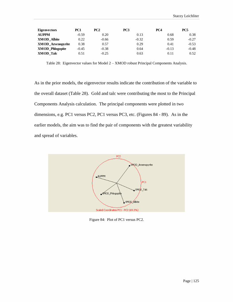
Stacey Leichliter

Page | 125

Eigenvectors PC1 PC2 PC3 PC4 PC5

AUPPM -0.59 0.20 0.13 0.68 0.38

XMOD_Albite 0.22 -0.66 -0.32 0.59 -0.27

XMOD_Arsenopyrite 0.38 0.57 0.29 0.41 -0.53

XMOD_Phlogopite -0.45 -0.38 0.64 -0.13 -0.48

XMOD_Talc 0.51 -0.25 0.63 0.11 0.52

Table 28: Eigenvector values for Model 2 – XMOD robust Principal Components Analysis.

As in the prior models, the eigenvector results indicate the contribution of the variable to

the overall dataset (Table 28). Gold and talc were contributing the most to the Principal

Components Analysis calculation. The principal components were plotted in two

dimensions, e.g. PC1 versus PC2, PC1 versus PC3, etc. (Figures 84 - 89). As in the

earlier models, the aim was to find the pair of components with the greatest variability

and spread of variables.


Stacey Leichliter

Page | 126




Stacey Leichliter

Page | 127



The first two plots (Figures 84 and 85) have the greatest spread of the variables, with the

first, PC1 versus PC2, having the largest (Figure 84). This spread of the variables

allowed for clustering of the data with similar multivariate characteristics. Data from the

PC1 versus PC2 plot was displayed in a multivariate scatter plot (Figure 90).

Stacey Leichliter

Page | 128

Figure 90: Multivariate scatter plot of PC1 versus PC2 for Model 2 – XMOD mineralogy by major rock

type.

As in Model 1 and Model 2 – Multi-Element, classes were constructed based on

clustering of the data with similar characteristics (Figures 91). There were three classes

identified: low plagioclase, high actinolite, and high talc. A discriminant diagram was

constructed based on these classes (Figure 92).

Each class then underwent non-linear regression modelling to predict recovery by bottle

roll test based on XMOD mineralogy (Table 29). The input minerals for the

Stacey Leichliter

Page | 129

Figure 91: Scatter plots of PC1 and PC2 along with different variables to identify the clusters

Stacey Leichliter

Page | 130

Figure 92: Discriminant diagram with classes for Model 2 – XMOD mineralogy (PC1 vs. actinolite).

regressions were chosen due to their strong correlation with the gold assay from the bottle

roll tests (extractable gold) and were gold (fire), K feldspar, muscovite, albite, and

chlorite.

Regression Equations for Model 2 - XMOD


High Actinolite AU1000_PPM_AASCL = (0.9701*AUPPM)+(0.2683*XMOD_K_feldspar)+-6.5647 5 1 15.17

Low Plagioclase AU1000_PPM_AASCL = (0.5762*AUPPM)+(0.5765*XMOD_K_feldspar)+(-0.4667*XMOD_Muscovite)+-9.0845 5 1 25.09

High Talc AU1000_PPM_AASCL = (1.0136*AUPPM)+(-0.4316*XMOD_Albite)+(-16.5011*XMOD_Chlorite(Fe)+3.8971 7 1 53.56

Table 29: Regression equations for Model 2 – XMOD.

The estimated bottle roll assays (extractable) were then compared against the measured

assay results. The average absolute error was calculated to be 34% overall for Model 2 –

Stacey Leichliter

Page | 131

XMOD mineralogy. The different classes had a wide variability in errors. The low

plagioclase had an average absolute error of 25%, high actinolite had 15%, and high talc

with 54%. More work is needed to constrain the variability with the high talc to reduce

the error.

6.3.4.3 Model 2 – Calculated Mineralogy

Another technique was used to model the bottle roll recovery for the Phase 1 samples.

This was calculated mineralogy from the multi-element assays by the technique described

in Hunt et al., 2012 and by a software program developed by researchers with AMIRA

P843A. The modelling methodology was consistent with those used to construct prior

models.

A correlation analysis determined the minerals related to the gold (fire) assay.

Correlations for the robust PCA were weaker (< 0.50 with gold). The input variables for

the PCA used in this were pyrite, albite, and actinolite (Table 30).

Robust Correlation AUPPM Pyrite albite actinolite

AUPPM 1.00 -0.03 -0.41 -0.01

Pyrite -0.03 1.00 -0.27 0.04

albite -0.41 -0.27 1.00 -0.01

actinolite -0.01 0.04 -0.01 1.00

Table 30: Correlations for the PCA for Model 2 - calculated mineralogy.

Stacey Leichliter

Page | 132

Eigenvectors PC1 PC2 PC3 PC4

AUPPM 0.59 0.45 0.30 -0.59

Pyrite 0.36 -0.68 -0.49 -0.41

albite -0.72 0.01 0.04 -0.70

actinolite 0.04 -0.58 0.82 0.00

Table 31: Eigenvectors for the PCA for Model 2 – calculated mineralogy.

The eigenvectors from the PCA analysis showed albite and gold having the largest

contribution in PC1 (Table 31). Plots of the principal components are shown in Figures

93 – 98.



Stacey Leichliter

Page | 133




Stacey Leichliter

Page | 134


The first, second, and fourth plots showed spreading of the variables, but the second plot

had the largest spread and variability (Figure 94). PC1 and PC3 were then plotted in a

multivariate scatter plot (Figure 99). Using the mineralogical data, cluster or groupings

of the data could be observed and classified (Figure 100).

Figure 99: Multivariate scatter plot of PC1 and PC3 for Model 2 – calculated mineralogy.

Stacey Leichliter

Page | 135

There were two classes identified within the clusters, high arsenopyrite and low

arsenopyrite (Figures 100 and 101). A discriminant diagram was constructed from these

classes (Figure 101).

Figure 100: Scatter plots to identify clusters for Model 2 – calculated mineralogy.

Figure 101: Discriminant diagram with classes from PCA for Model 2 – calculated mineralogy (PC1 vs.

PC3).

Stacey Leichliter

Page | 136

A regression model was calculated for each class to estimate the recovery by bottle roll

test (extractable gold) (Table 32). The input parameters were the minerals which were

the strongest when correlated with the gold assay from the bottle roll test. They were

gold, plagioclase, pyrite, albite, and actinolite.

Regression Equations for Model 2 - calculated mineralogy


High Arsenopyrite AU1000_PPM_AASCL = (-0.1074*AUPPM)+(0.1922*Feld_Pla)+(-0.9931*S_Pyrite)+14.6251 4 1 15.81

Low Aresenopyrite AU1000_PPM_AASCL = (1.0249*AUPPM)+(-0.02064*albite)+(-0.1367*actinoli)+-0.6867 13 0.99 14.27

Table 32: Regression equations for the calculated mineralogy model for Model 2.

The estimated bottle roll assay values were compared to the measured bottle roll test data.

An average absolute error for Model 2 – calculated mineralogy was found to be 15%

overall, with the high arsenopyrite class with an error of 16% and low arsenopyrite with

an error of 14%. This was slightly more than Model 2 – multi-element, but lower than

Model 2 – XMOD mineralogy.

6.3.5 Results

Model 1 was constructed using approximately 650 samples (gold > 0.3 g/t) that had both

recovery data (e.g. results of shake leach tests) and multi-element assay data. The

regression models showed a high strength of fit (R2

> 0.96) and an average relative error

of ~11% when compared to the analytical error of the tests (fire assay and shake leach

assay) (< 10%). When the measured shake leach recovery was plotted against the

measured shake leach recovery (ppm) (Figure 102), it showed that the calculated gold

Stacey Leichliter

Page | 137

recovery was between 70% and 90% while the measured shake leach recovery had a

greater spread or more variability with values between 40% and 100%.

y = 0.049x + 77.177

0

20

40

60

80

100

0 20 40 60 80 100

calc

ula

ted

re

cove

ry (

%)

measured recovery (%)

Model 1 Gold Recovery (%)

Gold Recovery

Linear (Gold Recovery)

Figure 102: Calculated versus measured gold recovery (%).

Looking at the gold grades as a possible cause of the larger errors in the calculated shake

leach recoveries (ppm), it appears that the higher gold grade, the greater the error (Figure

103). This could be that the coarser or larger gold grains aren’t completely leaching with

the cyanide. Ore with the higher gold grades may need longer time to leach or even

another extraction process, such as gravity concentration.

0

2

4

6

8

10

12

0 2 4 6 8 10

calc

ula

ted

re

cove

ry (

pp

m)

measured recovery (ppm)

Recovery by gold grade

SLAu <1ppm

SLAU 1 to <3ppm

SLAU >3ppm

Figure 103: Calculated versus measured gold recovery (ppm) divided by gold grade.

Stacey Leichliter

Page | 138

A simple linear regression model was calculated using the fire assay and the measured

shake leach assay data (Figure 104), so this model would be considered the simplest

model to predict recoverable gold. The regression analysis equation to predict cyanide

recoverable gold was:

AuSL(ppm) = 0.6331*Au(ppm)+0.103

y = 0.6331x + 0.103R² = 0.9484

0

2

4

6

8

10

0 2 4 6 8 10 12 14

Me

asu

red

SLg

old

ass

ay (

pp

m)

Fire (head) gold grade (ppm)

Linear Regression Model

Linear Regression

Linear (Linear Regression)

Figure 104: Linear regression model to predict cyanidable gold.

An F –test was performed on the first recovery model and a linear recovery model based

on the prior testwork (Figures 105 and 106). An F-test allows for the comparison of two

different models to determine which model is best fitted to the data. The result was 45%,

meaning Model 1 was a moderate improvement over simply using a linear recovery

model.

Stacey Leichliter

Page | 139

y = 0.9258x + 0.083R² = 0.9422

0

2

4

6

8

0 2 4 6 8

calc

ula

ted

re

cove

ry (

pp

m)


Model 1

All samples

Linear (All samples)

Figure 105: Calculated versus measured gold recovery (ppm) as determined by Model 1.

y = 0.9484x + 0.0454R² = 0.9484

0

2

4

6

8

0 2 4 6 8

calc

ula

ted

re

cove

ry (

pp

m)


Linear regression model

All samples

Linear (All samples)

Figure 106: Calculated versus measured gold recovery (ppm) as determined by a linear model.

Stacey Leichliter

Page | 140

The average absolute error for Model 1 was approximately 11%, and the average absolute

error for the simple linear model was 10%. The difference in absolute errors is

negligible. The estimated shake leach assays were then wireframed and compared with

Model 1’s wireframes (Figure 107). There was noticeable difference in the wireframes,

which could be due to the mineralogical aspects used in the geometallurgical model

(Model 1).

Figure 107: Estimated shake leach recoveries using a simple linear model in the same domains with

lithologies (purple = Hornfels, blue = Early Diorites, and pink = Intermineral Diorites).

Model 2 was constructed using only 17 high grade gold samples (> 7.0 g/t Au) that had

recovery data (e.g. results of bottle roll tests) along with multi-element assay data,

XMOD mineralogy, and calculated mineralogy. The average relative errors for the

different Model 2 methods were 14%, 34%, and 15%, respectively. Model 2 – multi-

element could be used to predict the gold recovery (cyanidability) of samples, but this

model had a larger error than Model 1 and needed to be strengthened by more data

points.

Stacey Leichliter

Page | 141

Next, the Phase 1 sample data was estimated using the bottle roll test recovery regression

equations and domained, using the same parameters as in Model 1 (low <70%, average

70%-85%, and high >85%). These domains were wireframed (3 dimensional views) to

visualize the variability in the estimated bottle roll gold recovery and to check spatial

continuity and relationships with the geology (Figure 108).

Figure 108: Estimated bottle roll recoveries for the Phase 1 samples in the same domains with lithologies

(purple = Hornfels, blue = Early Diorites, and pink = Intermineral Diorites).

When comparing the location of the gold recovery domains with lithology maps, the

wireframes overlapped the major lithologies (Figures 7 and 108). The low recovery areas

compared with the location of early diorite lithologies (Figures 7 and 108). The areas

with high gold recovery by bottle rolls corresponded with areas underlain by the

intermineral diorites (Figures 7 and 108). The results of this study suggested that much

of the La Colosa ore (with the exception of mineralisation hosted in the early diorites)

may be amenable to gold extraction via cyanide leaching.

Stacey Leichliter

Page | 142

6.3.6 Summary

Model 1 was based on regression model equations which were used to estimate the gold

recovery by shake leach testing on samples that range from the cut-off value of 0.3 g/t Au

to 7.6 g/t Au. The gold recoveries were calculated and domained into rankings based on

natural statistical breaks of the data. The domains were wireframed and spatially

compared to the geologic model. The areas of low recovery were associated with the

early diorites and high recovery was associated with the intermineral diorites.

Model 2 was designed to estimate gold recovery by bottle roll tests. This model was

constructed with data of samples from Phase 1 (Au grade >7 g/t). The bottle roll gold

recoveries were calculated using various data sources (i.e. multi-element assays, XMOD

mineralogy, and calculated mineralogy), but the model with the lowest absolute relative

error was the one that used multi-element assays (14%). The estimated bottle roll gold

recoveries were modelled, classified, calculated, domained, and then wireframed to check

spatial continuity. The areas of high and low recoveries were associated with early

diorites and intermineral diorites, respectively.

The elements that were correlated with the fire (head) assays and shake leach and bottle

roll assays (cyanide extractable gold) in the PCA and regression equations have a

mineralogical relationship with the gold mineralisation as discovered in the gold

deportment study. Calcium, sodium, potassium, and sulfur are related to the calcic-sodic,

potassic, and potassic-calcic alteration assemblages (actinolite, albite, K feldspar,

Stacey Leichliter

Page | 143

biotite/phlogopite and pyrite minerals). Silver and tellurium are associated with the gold

grades due to the presence of gold tellurides and gold-silver tellurides.

Two types of cyanide gold recovery models were created. The shake leach gold

recovery model (Model 1) had the lower absolute relative error (11%) on a larger data set

(n = 647). With over 600 samples in the model, the shake leach gold recovery model

(Model 1) was the stronger model. It also represented a wider range of the gold grades,

not just the higher grades (>7 g/t Au).

Model 1 showed a moderate improvement from a simple, linear model (45%), which

suggested that the complex domain based geometallurgical model was not

overwhelmingly better than a simple linear regression. This could be due to the fact that

a majority of the variability in the recoverable gold is correlated with the fire (head) gold

grade (~63%). While the estimation using the linear regression model is more efficient

than the complex geometallurgical model, it doesn’t consider the mineralogical traits

which cause the variability.

Stacey Leichliter

Page | 144

Chapter 7: Geometallurgical Recovery Model

and Conclusions

7.1 Geometallurgical Recovery Model

The goal of this project was to develop a geometallurgical recovery model using the gold

mineralogy, analytical data, and recovery data. This was accomplished by applying the

modelling techniques stated in section 6.3.4. Model 1 incorporated samples with known

shake leach gold recoveries, and Model 2 utilised samples with measured bottle roll gold

recoveries for the Phase 1 samples. Phase 2 samples did not have any recovery testwork

available, so they were used to build the geometallurgical recovery model. Phase 2

samples were also used in the site’s metallurgical variability testwork.

In Chapter 6, geometallurgical gold recovery models (cyanidation) were constructed

using two types of analytical testwork data that represented cyanide extractable gold,

shake leach gold assays and bottle roll assays. The shake leach gold recovery model

(Model 1 – Section 6.3.2) included samples with gold grades from 0.3 g/t to >7 g/t. The

bottle roll gold recovery model (Model 2 – Section 6.3.3) was built using samples that

had high grade gold (>7 g/t). The goal of the geometallurgical recovery model was to

identify and constrain the variability in the recoveries by cyanidation. Since variability

was the key to the project, a complex geometallurgical model was preferred over the

simple linear regression model and mineralogical aspects can aid in identifying the causes

of the variability.

Stacey Leichliter

Page | 145

Gold grades for Phase 2 samples ranged from 0.3 g/t to 4.8 g/t, so the Model 1, which

was developed using samples with lower gold grades ( > 0.3 g/t), seemed more suitable to

utilise for the gold recovery estimations. . Model 2 was constructed using high gold

assay values (> 7 g/t), but had no lower gold grades. This was a problem because the

lower gold grades were not modelled.

In the construction of Model 1, a discriminant diagram was built with the classes which

represent the clusters apparent in the data set. Using the diagram from Model 1, the new

data was easily imported, and the data was analysed and classified based on the

discriminant diagram.. The data from the Phase 2 samples plotted on the Model 1

recovery diagram is shown in Figure 109.

Figure 109: Phase 2 sample data plotted on the Model 1 discriminant diagram (PC1 vs. PC3).

Stacey Leichliter

Page | 146

Figure 110: Phase 2 sample data clusters classified by the Model 1 discriminant diagram (PC1 vs. PC3).

By applying those methods and calculations, it was observed that the data points were

relatively evenly spread between the four classes (high K = 14 samples, low Te = 13

samples, high Ca = 15 samples, and average mineralogy = 8 samples) on the

classification diagram (Figures 109 and 110).

The geometallurgical shake leach gold recovery model (Model 1) was applied to the

Phase 2 samples. Sample data was subjected to the same methods and calculations used

in Model 1 (Section 6.3.2). The regression equations developed in Model 1 were then

used to estimate the shake leach gold assays (Table 23).Measured gold recovery values

were not yet available for Phase 2 samples, so this model could not be verified at this

Stacey Leichliter

Page | 147

Figure 111: Wireframes of Phase 2 samples with estimated shake leach recovery domains: low = <70%

(red), average = 70%-85% (green), and high = >85% (yellow).

When comparing the wireframes of the Phase 2 estimated shake leach gold recoveries

with those of Model 1 (Figure 108), there was some difference. Mainly, the high

recovery domain was smaller than Model 1(Figure 111). The average and low recovery

domains were consistent with Model 1. Differences in the wireframes could possibly be

due to average relative error in the geometallurgical model. Also, there were fewer data

points to wireframe than Model 1 (50 samples versus 650 samples) which could cause

differences in the construction of the wireframes.

7.2 Conclusions

The La Colosa porphyry gold deposit is unique due to its high gold grades with low to

barren amounts of copper (< 0.034%) and molybdenum (< 0.004%) (Lodder et al., 2010).

The bulk of the gold mineralisation is located within early diorite porphyry (Lodder et al.,

2010). The alteration assemblages that appear to correlate with the gold mineralisation

Stacey Leichliter

Page | 148

are the potassic and potassic-calcic. These assemblages have secondary biotite, K

feldspar, sulfides (pyrite), with or without actinolite (potassic-calcic). The two major

vein types associated with the gold mineralisation, quartz-sulfide and sulfide, are related

to the potassic and potassic-calcic assemblages. This linkage between the potassic

alteration assemblages and the major vein types associated with the gold mineralisation is

consistent with the current models for gold porphyry deposits (Sillitoe, 2000). Gold

mineralisation appears to be both disseminated (vein poor) and vein-related (vein rich) in

the early diorites, but vein-related in the intermineral diorites and dacites. This suggests

there are multiple gold mineralisation events, and these alteration events are related to the

potassic and potassic-calcic alteration events.

The deportment of the gold mineralisation at La Colosa is varied. The types of gold

mineralisation include native gold, gold tellurides, and gold-silver tellurides. Gold in the

overall deposit is very fine-grained, associated with pyrite and feldspars, and includes a

minor amount of free gold. The variability in the gold mineralisation can aid in

understanding the variability in the recovery data.

Understanding and constraining the variability helps identify the gold’s character using

parameters such as mineralogy or elemental assays. These parameters can then be used

to divide the data into classes and then calculate the estimated recovery for each class.

These estimations are then applied to the entire drill hole database, domained, and

wireframed. The model provides input into the resource block model. The estimated

Stacey Leichliter

Page | 149

recoveries provide a prediction of the recovery variability which could occur in the

deposit.

When the domained geometallurgical model was compared with a simple linear

regression model using the fire assay and measured shake leach gold assay, the more

complex geometallurgical model was not significantly better than the linear model. The

average absolute errors were similar and the F-test yielded only a 45% improvement for

the complex model. In this study, it may be more efficient to use the simple, linear model

rather than the more complex geometallurgical model. The goal of this study was to

understand and constrain the variability of the gold recovery at La Colosa, and this was

more evident using the geometallurgical model, Model 1.

By using estimation tools to produce a geometallurgical model to predict gold recovery, it

is possible to provide faster, abundant information on the variability of the deposit. The

predictive geometallurgical model, or the simple linear regression model, can be

regularly updated with new data as further testwork and analysis will be performed.

These models are dynamic methods to provide information to a mine site, so these

models may be pro-active in their decisions on operations.

7.3 Further Work

The study of the genesis of the porphyry gold deposit at La Colosa is in its infancy, and

more knowledge of the intrusions and structural controls are necessary. Gold

mineralisation events at La Colosa have not been studied. Information on the types of

Stacey Leichliter

Page | 150

phases of the different pulses of gold bearing fluids would aid further understanding of

gold deportment and contribute data towards geometallurgical modelling. Further work

on the predictive geometallurgical recovery model for the La Colosa gold deposit would

include a trade off study using gravity, flotation, and cyanidation. Information on the

mineralogy of the feed and tails of the different recovery techniques would also be

beneficial for strengthening the geometallurgical recovery model. This mineralogy

information is important, because it can show the types and grain sizes of the gold

mineralisation that reports to each process.

The developed predictive geometallurgical shake leach gold recovery model will need to

be updated with new data and testwork analysis as they become available. The additional

data may aid in strengthening the geometallurgical model as more information is gained

about the gold recovery. As additional data for the bottle roll testwork is available, the

model for the gold recovery estimation using bottle rolls (Model 2) will need to be

revised. Each model will need to be reiterated and revised as more gold recovery data is

acquired and the model is tested. Until the more complex geometallurgical model is

stronger than it is currently, the simple linear model is sufficient to estimate the cyanide

recoverable gold at La Colosa, although the variability of the gold recovery is more

difficult to constrain.

Stacey Leichliter

Page | 151

References

ALS, 2012, written communication (email) on analytical laboratory assay testwork

procedures and analytical testwork errors.

AngloGold Ashanti, 2010, Mineral Resource and Ore Reserve Report 2010., URL

data:http://www.anglogoldashanti.co.za/subwebs/InformationForInvestors/Report

s10/financials/files/AGA-resource-reserves-2010.pdf.

AngloGold Ashanti Colombia, 2010, La Colosa Logging Manual, AngloGold Ashanti

internal report. 13 p.

AngloGold Ashanti Colombia, 2011, Geologic Map, AngloGold Ashanti internal

report.

Aspden, J.A., McCourt, W. J., and Brook, M., 1987, Geometrical control of

subduction-related magmatism: The Mesozoic and Cenozoic plutonic

history of western Colombia, Journal of the Geological Society of London, v. 144,

p. 893-905.

Berry, R., 2010, Review of trace-element mapping using a laser ablation sourced,

induction-coupled-plasma quadrupole mass spectrometer (LA-ICP-MS) at

CODES, AMIRA GeMiii

Technical Report 4, Confidential report. 3 p.

Berry, R. and Hunt, J., 2011, Grain Size in GeoMetallurgy – Review of Progress,

AMIRA GeMiii

Technical Report 8, Confidential report. 15 p.

Berry, R, Hunt, J., and McKnight S., 2011, Estimating Mineralogy in Bulk

Samples, First AusIMM International Geometallurgy Conference 2011,

Conference Proceedings, AusIMM, Brisbane, Australia, 4 p.

Campbell, N.A., 1980, Robust procedures in multivariate analysis. I: Robust covariance

estimation. Applied Statistics, v. 29, p. 231-237.

Cediel, F. and Cáceres, C., 2000, Geologic map of Colombia, Geotec Ltd., Third

Edition, Digital Format with Legend and Tectono-Stratigraphic Chart.

Cediel, F., Shaw, R.P., and Cáceres, C., 2003, Tectonic assembly of the Northern

Andean block, in Bartolini, C., Buffler, R.T., and Blickwedw, J., eds., The

Circum-Gulf of Mexico and Caribbean: Hydrocarbon habitats, basin formation,

and plate tectonics, American Association of Petroleum Geologists Memoir v. 79,

p. 815-848.

http://www.anglogoldashanti.co.za/subwebs/InformationForInvestors/Reports

http://www.anglogoldashanti.co.za/subwebs/InformationForInvestors/Reports

Stacey Leichliter

Page | 152

Davis, J.C., 2002, Statistics and Data Analysis in Geology, John Wiley and Sons,

New York, Third edition, 638 p.

Essa, 2012, http://www.essa.com.au/EssaProductsDetail

FEI, 2012, http://www.fei-natural-resources.com/uploadedFiles/Documents

Private/Content/HR_DS_MLA650.pdf

Fournier, R.O., 1999, Hydrothermal processes related to movement of fluid from

plastic into brittle rock in the magmatic-epithermal environment, Society of

Economic Geologists, Economic Geology, v. 94, p. 1193-1211.

Fuerstenau, M.C. and Han, K.N., 2003, Principles of Mineral Processing, Society for

Mining, Metallurgy, and Exploration, Inc., Littleton, Colorado, 573 p.

Garcia-Bernal, C.A., 2011, Review of gold-rich porphyry deposits of the Northern

Andes, with special emphasis on the Colosa Gold Porphyry, Colombia, and its

comparison with the Central Andes gold-rich porphyry province, Thesis, Rhodes

University.

Gehrels, G.E., Valencia, V.A., and Ruiz, J., 2008, Enhanced precision, accuracy,

efficiency, and spatial resolution of U-Pb ages by laser ablation-multi-collector-

inductively coupled plasma-mass spectrometry, Geochemistry Geophysics

Geosystems, v. 9, Q03017, 13 p.

Gil-Rodríguez, J., 2010, Igneous Petrology of the Colosa Gold-Rich Porphyry

System (Tolima, Colombia), Thesis, University of Arizona, p. 1-51.

Goossens, P.J., 1976, Lithologic, Geochemical, and Metallogenic Belts in the

Northern Andes, and Their Structural Relationships, Society of Mining Engineers,

Transactions, v. 260, p. 60-67.

Gu, Y., 2003, Automated Scanning Electron Microscope Based Mineral Liberation

Analysis: An Introduction to JKMRC/FEI Mineral Liberation Analyser, Journal

of Minerals & Materials Characterization & Engineering, v. 2, no.1, p. 33-41.

Gustafson, L.B. and Hunt, J.P., 1975, The porphyry copper deposit at El Salvador,

Chile, Society of Economic Geologists, Economic Geology, v. 70, p. 857-912.

Horner, J., 2011, Structural Geological Study (PFS) Final Report for La Colosa

Gold Mine, iC consulenten group, AngloGold Ashanti internal report. 58 p.

Hunt, J., Berry, R., Montoya, P., Leichliter, S., Triffett, B., and Rocha, M., 2012, Geomet

2012 proceedings, Santiago, Chile.

ioGAS, 2011, version 4.4, ioGlobal, http://iogas.net

http://www.essa.com.au/EssaProductsDetail

http://www.fei-natural-resources.com/uploadedFiles/Documents

http://iogas.net/

Stacey Leichliter

Page | 153

Irving, E.M., 1971, La evolution structural de los Andes más septentrionales de

Colombia: Boletín Geol. INGEOMINAS, v. 19, no. 2, p. 1-89.

Keeney, L., 2010, The Development of a Novel Method for Integrating

Geometallurgical Mapping and Orebody Modelling, PhD Thesis, University of

Queensland.

Kennan, L. and Pindell, J., 2009, Dextral shear, terrane accretion and basin

formation in the northern Andes: Best explained by interaction with a Pacific-

derived Caribbean Plate, Geological Society of London, Special Publications,

v. 328, p. 487-532.

Leal-Mejia, H., 2010, Regional metallogenic study applied to exploration of gold

mineralisation in the San Lucas, Antioquia and Cauca Canyon regions of

Colombia, South America., PhD. Thesis, University of Barcelona.

Leapfrog 3D, 2011, version 2.4.4, ARANZ Geo Limited.,

http://www.leapfrog3d.com/mining

Lodder, C., Padilla, R., Shaw, R., Garzon, T., Palacio, E., and Jahoda, R., 2010,

Discovery History of the La Colosa Gold Porphyry Deposit, Cajamarca,

Colombia, Society of Economic Geologists Special Publication, v. 15, p. 19-28.

Lozano, O., 1984, Prospección geoquímica para oro, plata, antimonio y mercurio

en los municipios de Salento, Quindio y Cajamarca, Tolima: Instituto Nacional

de Geologia y Minas de Colombia, Boletín Geologico, v. 27, p. 4-76.

Marsden, J.O. and House, C.I., 2006, The Chemistry of Gold Extraction, Second

Edition, Society of Mining, Metallurgy, and Exploration, Inc., Littleton,

Colorado, 651 p.

Maya, M. and González, H., 1995, Unidades Litodémicas en la Cordillera Central

de Colombia: Boletín Geologico INGEOMINAS, v. 35, no. 2-3, p. 43-57.

McCourt, W.J., Aspden, J.A., and Brook, M., 1984, New geological and

geochronological data from the Colombian Andes: Continental growth by

multiple accretion: Journal of the Geological Society of London, v. 141, p. 831-

845.

Montoya, P., 2012, Geometallurgical Mapping and Mine Modelling - Comminution

Studies: La Colosa Case Study, AMIRA P843A, Thesis, University of

Queensland.

Muntean, J.L. and Einaudi, M.T., 2000, Porphyry Gold Deposits of the Refugio

District, Maricunga Belt, Northern Chile, Society of Economic Geologists,

Economic Geology, v. 95, p. 1445-1472.

Stacey Leichliter

Page | 154

Núñez, A., 2001, Memoria Explicativa Mapa Geologico del Departamento del

Tolima, INGEOMINAS, 101 p.

Optics Planet, 2012, http://www.opticsplanet.com/eberbach-heavy-duty-shaker-two-

speed-eberbach-6010.html

Pindell, J.L. and Kennan, L., 2001, Kinematic evolution of the Gulf of Mexico and

Caribbean: Gulf Coast Section Society of Economic Paleontologists and

Mineralogists Foundation, 21st Annual Research Conference Transactions,

Petroleum Systems of Deep-Water Basins, p. 193-220.

Pindell, J.L. and Kennan, L., 2009, Tectonic evolution of the Gulf of Mexico,

Caribbean and Northern South America in the mantle reference frame: An

update, in James, K.H., Lorente, M.A., and Pindell, J.L., eds., The Origin and

Evolution of the Caribbean Plate, Geological Society of London, Special

Publications, v. 328, p. 1-55.

Proffett, J.M., 2003, Geology of the Bajo de la Alumbrera Porphyry Copper-Gold

Deposit, Argentina, Society of Economic Geologists, Economic Geology, v. 98,

p. 1535-1574.

Pulido, O.H., 1988, Geología y geoquímica del área de San Antonio, Cajamarca,

Tolima, Boletín Geológico INGEOMINAS, v. 29, no. 2, p. 37-84.

Redmond, P.B. and Einaudi, M.T., 2010, The Bingham Canyon Porphyry Cu-Mo-Au

Deposit. I. Sequence of Intrusions, Vein Formation, and Sulfide Deposition,

Society of Economic Geologists, Economic Geology, v. 105, p. 43-68.

Regression Diagnostics, 2012, http://rguha.net/writing/notes/stats/node6.html

Sadalmelik, I., 2007, Topographic map of Colombia, Colombia Topography.png,

http://commons.wikimedia.org/wiki/File:ColombiaTopography.png

Sasso, A.M., 1997, Geological evolution and metallogenetic relationships of the

Farallon Negro volcanic complex, NW Argentina, Unpublished PhD. Thesis,

Kingston, ON, Canada, Queens University, 842 p.

Sasso, A.M. and Clark, A. II., 1998, The Farallón Negro Group, northwestern

Argentina: Magmatic, hydrothermal and tectonic evolution and implications for

Cu-Au metallogeny in the Andean back-arc, Society of Economic Geologists

Newsletter, v. 34, p. 1, 8-18.

Seedorff, E., Barton, M., Stavast, W., and Maher, D.J., 2008, Root Zones of

Porphyry Systems: Extending the Porphyry Model to Depth, Society of


http://www.opticsplanet.com/eberbach-heavy-duty-shaker-two-

http://commons.wikimedia.org/wiki/File:ColombiaTopography.png

Stacey Leichliter

Page | 155

SGS, 2012, http://www.sgs.com/en/Mining/Metallurgy-and-Process-Design/

Cyanidation-Technologies/Cyanide-Leaching/Cyanide-Bottle-Roll-Test.aspx

Sillitoe, R.H., Jaramillo, L., Damon, P.E., Shafiqullah, M., and Escovar, R., 1982,

Setting, Characteristics, and Age of the Andean Porphyry Copper Belt in

Colombia, Society of Economic Geologists, Economic Geology, v. 77, p. 1837-

1850.

Sillitoe, R.H., Jaramillo, L., and Castro, H., 1984, Geologic Exploration of a

Molybdenum-Rich Porphyry Copper Deposit at Mocoa, Colombia, Society of


Sillitoe, R.H., 2000, Gold-Rich Porphyry Deposits: Descriptive and Genetic Models

and Their Role in Exploration and Discovery, Society of Economic Geologists,

SEG Reviews, v. 13, p. 315-345.

Sillitoe, R.H., 2007, Preliminary Geological Model for the Colosa Porphyry Gold

System: Bogota, Colombia, AngloGold Ashanti, Internal Report, 13 p.

Sillitoe, R.H., 2008, Major Gold Deposits and Belts of the North and South

American Cordillera: Distribution, Tectonomagmatic Settings, and Metallogenic

Considerations, Society of Economic Geologists, Economic Geology, v. 103, p.

663-687.

Sillitoe, R.H., 2010, Porphyry Copper Systems, Society of Economic Geologists,

Economic Geology, v. 105, p. 3-41.

Taboada, A., Rivera, L.A., Fuenzalida, A., Cisternas, A., Philip, H., Bijwaard, H.,

Olaya, J., and Rivera, C., 2000, Geodynamics of the Northern Andes:

Subductions and Intracontinental deformation (Colombia): Tectonics, v. 19, no.

5, p. 787-813.

Thorne, J., 2011, ftp://statgen.ncsu.edu/pub/thorne/molevoclass/

AtchleyOct19.pdf

Ulrich, T. and Heinrich, C., 2002, Geology and Alteration Geochemistry of the

Porphyry Cu-Au Deposit at Bajo de la Alumbrera, Argentina, Society of


Vila, T., Sillitoe, R.,Betzhold, J., and Viteri, E., 1991, The Porphyry Gold Deposit

at Marte, Northern Chile, Society of Economic Geologists, Economic Geology,

v. 86, p. 1271-1286.

Wills, B.A. and Napier-Munn,T.J., 2006, Wills’ Mineral Processing Technology,

Seventh Edition, Elsevier Ltd, 444 p.

http://www.sgs.com/en/Mining/Metallurgy-and-Process-Design/

Stacey Leichliter

Page | 156

Vitae

Stacey Leichliter

Page | 157

Stacey Leichliter

671 Calico Court

Woodland Park, CO 80863

(573)465-0449

[email protected]

OBJECTIVE: Geometallurgist position with a company.

SUMMARY: • Masters of Science in Geology.

• Bachelor of Science in Geology.

• Minor in Geological Engineering.

• Computer Applications include: Vulcan, LeapFrog 3D, ArcMap,

ioGAS, Century Systems, MS Office, Windows XP and 7, and the

Internet.

EDUCATION: Bachelor of Science in Geology (2006)

University of Missouri- Rolla, Rolla, Missouri

Major: Geology Minor: Geological Engineering

Masters of Science in Geology (2011-present)

University of Tasmania – Hobart, Tasmania, Australia

Thesis: “Gold Deportment and Geometallurgical Recovery Model

for the La Colosa, Porphyry Gold Deposit, Colombia”

GEOLOGY

EXPERIENCE:

Geometallurgist - AngloGold Ashanti (Colorado) Corp. / Cripple Creek &

Victor Gold Mine (Jan. 2012 to present)

• Plan and budget Geometallurgy Program at CC&V

• Study current recovery methods and domains

• Construct models to predict leach behaviour

• Construct models to predict gravity and flotation behaviour

• Construct models to show hardness variability of the rock

• Aid process, mill, resource, ore control, and other department with

predictive models and tests

• Construct predictive recovery models for La Colosa

Exploration Geologist - AngloGold Ashanti (Colorado) Corp. / Cripple

Creek & Victor Gold Mine (Jan. 2007-Dec. 2011)

• Supervise exploration drill rigs (both diamond drill core and reverse

circulation)

• Plan and execute drill holes

• Geological and geotechnical logging of core and RC chips

• Provided site specific safety training to drillers

• Construction of drill pads with aid of excavation crew

Stacey Leichliter

Page | 158

• Modelling projects using Vulcan to define rock types and structures

in the subsurface

• Prepare reports for the company and the state

• Supervise environmental monitoring well installations

PUBLICATIONS: Leichliter, S., Hunt, J., Berry, R., Keeney, L., Montoya, P., Chamberlain, V.,

Jahoda, R., and Drews, U., 2011, Development of a Predictive

Geometallurgical Recovery Model for the La Colosa, Porphyry Gold

Deposit, Colombia, Proceedings from the First AusIMM International

Geometallurgy Conference 2011, Brisbane, Australia.

Montoya, P., Keeney, L., Jahoda, R., Hunt, J., Berry, R., Drews, U., Chamberlain, V.,

and Leichliter, S., 2011, Development of a Predictive Geometallurgical

Recovery Model for the La Colosa, Porphyry Gold Deposit, Colombia,

Proceedings from the First AusIMM International Geometallurgy

Conference 2011, Brisbane, Australia

ACTIVITIES: • SME 2007- present

• Geological Society of America 2006-present

• SEG 2008- present

• AusIMM 2011- present

Stacey Leichliter

Page | 159

Appendix A

Shake Leach Assay Information

Stacey Leichliter

Page | 160

Analysis of Gold by Shake (Cyanide) Leach (SGS certified laboratory)

1. Parameter(s) measured, unit(s):

Gold (Au): ppm

2. Typical sample size:

15- 25g

3. Type of sample applicable (media):

Pulverised and crushed rocks (85% passing 75µm 200 mesh)

4. Sample preparation technique used:

Crushed and pulverised rock samples are leached using a 0.5 % Sodium cyanide (NaCN)

in a solution of 0.25% NaOH and agitated for 1 hour. The sample is centrifuged to obtain

the supernatant which is decanted and submitted for analysis.

5. Method of analysis used:

The leached sample solution is analysed by Flame Atomic Absorption Spectrometer

(AAS) or inductively coupled plasma Optical Emission Spectrometer (ICP-OES).

Samples are analysed against known calibration materials to provide quantitative analysis

of Au (standards).

Data reduction by:

The results are exported via computer, on line, data fed to the SGS Laboratory

Information Management System (SLIM) with secure audit trail.

6. Figures of Merit:

Element Detection Limit ppm

Au 0.03ppm

7. Quality control:

Instrument calibration is performed for each batch or work order and calibration checks

are analysed within each analytical run. Quality control materials include method blanks,

replicates, duplicates and reference materials and are randomly inserted with the

frequency set according to method protocols at ~14%.

Quality assurance measures of precision and accuracy are verified statistically using

SLIM control charts with set criteria for data acceptance. Data that fails is subject to

investigation and repeated as necessary.

Stacey Leichliter

Page | 161

Appendix B

Bottle Roll Information

Stacey Leichliter

Page | 162

Gold by Bulk Extended Leach Cyanide (Bottle Roll) (ALS certified laboratory)

1. Parameter(s) measured, unit(s):

Gold (Au): ppm

2. Typical sample size:

1,000g

3. Type of sample applicable (media):

Pulverised and crushed rocks (85% passing 75µm 200 mesh)

4. Sample preparation technique used:

Sample is placed into a polyethylene bottle, jar, or drum to which a 0.25% NaCN leach

solution is added. The container is subsequently shaken to wet the sample thoroughly,

and then rolled for up to 24 hours.

5. Method of analysis used:

Atomic Absorption Spectroscopy (AAS). After rolling, a portion of the leached sample

solution or leachate is withdrawn, centrifuged until clear, and immediately analysed by

atomic absorption spectroscopy against matrix matched gold standards.

6. Figures of Merit:

Elemental Detection Limit

Au 0.01ppm

7. Quality control:

Instrument calibration is performed for each batch or work order and calibration checks

are analysed within each analytical run. Quality control materials include method blanks,

replicates, duplicates and reference materials and are randomly inserted with the

frequency set according to method protocols.

Quality assurance measures of precision and accuracy are verified statistically control

charts with set criteria for data acceptance. Data that fails is subject to investigation and

repeated as necessary.

Stacey Leichliter

Page | 163

Appendix C

Laser Ablation (LA-ICP-MS) Information

Stacey Leichliter

Page | 164

Laser ablation (LA-ICP-MS) Information (Berry, 2009)

1. Technologies

Laser microprobe, interface, and ICPMS

2. Sample size

Resin block (25mm)

3. Type of sample (media)

Whole or crushed rock mounted in resin block (25mm)

4. Methodology

Sample is placed into the sample chamber, which sits below the laser, and is flushed with

argon (Ar) gas. Helium (He) gas is then bled into a small sample enclosure. The laser is

turned on and begins to ablate the surface of the sample (depth of about 50 µm). Pre-

ablation of the sample also may be chosen to eliminate any possible sample preparation

contamination. As the sample is ablated, fine particles are carried by the He and Ar gases

into a set of plastic tube and into the plasma. At the plasma, the particles are vaporized

and ionized before entering a quadruple mass spectrometer. This mass spectrometer

measures various atomic weights of ions in the sample.

5. Detection Limit

0.1 – 20 ppm with some heavy elements capable of ppb

Typical LA-ICP-MS instrument

Stacey Leichliter

Page | 165

Appendix D

Detailed Geologic Logs (Digital)

Stacey Leichliter

Page | 166

Appendix E

Photographs (Digital)

Stacey Leichliter

Page | 167

Appendix F

MLA Data (Digital)

Stacey Leichliter

Page | 168

Appendix G

Recovery Data (Digital)

Stacey Leichliter

Page | 169

Appendix H

Mahalanobis Distance

Stacey Leichliter

Page | 170

Mahalanobis Distance

Background

In univariate statistics, analysis is performed on a single variable, such as gold. With

multivariate statistics, analysis is performed on more than one variable, e.g. gold,

tellurium, potassium (Davis, 2002 and ioGAS, 2011). To determine the similarity

between the data, standard deviations are used in univariate statistics, and Mahalanobis

Distance can be used in multivariate statistics (Davis, 2002).

The Mahalanobis Distance (M-dist or MD) is the distance of a data point from the

centroid, or ”mean point” in multidimensional space, defined by other compared

variables. This can give an indication if a sample is an outlier with respect to the other

independent, compared variables (Regression Diagnostics, 2012).

The Mahalanobis Distance is calculated using the following equation:

MD = ((hi-10/N)/ (1-hi))*((N (N-2))/ (N-1)

MD = Mahalanobis Distance

hi = Distance between X values and the means of all X values

N = number of data

ioGAS Methods

Using the software program ioGAS, this calculation can be performed by selecting

variables which correlate. The compute Mahalanobis Distance tool is located under the

Analysis header.

Stacey Leichliter

Page | 171

1. The parameters need to be selected, e.g. “Transformation”, “Outlier” cut-off (Chi-sq)”,

“Algorithm”, “By colour group”, “All rows”, and “Show probability plot”.

2. This calculation is best when performed on normally distributed data, so a transformation

may be needed to give it a more normal distribution.

3. The “Outlier cut-off (Chi-sq)” determines the percentile of data which is considered

normal, not an outlier.

4. The “Algorithm” field determines the level of outlier rejection. A lower rejection level

allows for more outliers.

5. If different populations, or colour groups, require independent Mahalanobis Distance

calculations, the option to perform by colour groups will need to be selected.

6. The “All rows” option allows for the calculation of the Mahalanobis Distance for all data,

not just the visible data.

7. A probability plot can be displayed when “Show probability plot” is selected.

8. After selecting the parameters, the names for the output columns (default is M-dist) will

need to be chosen.

9. Two output columns are created, one for outliers and the other for the normal data. The

data can be exported into a .csv file (ioGAS, 2011).

A robust Mahalanobis Distance calculation can be used when there is a possibility of

having atypical data which could affect the calculation. The robust calculation gives less

weight to the extreme or atypical values. This is a special ioGAS algorithm which is

Stacey Leichliter

Page | 172

discussed in the article by Campbell, 1980 (ioGAS, 2011). The robust calculations can

allow for the removal of high, medium, or low sample outliers before the calculation

(ioGAS, 2011).

Stacey Leichliter

Page | 173

Appendix I

Principal Components Analysis

Stacey Leichliter

Page | 174

Principal Components Analysis

Background

Principal Components Analysis (PCA) is a multivariate statistical technique that takes a

group of compared variables and calculates linear transformations under optimal

conditions (Davis, 2002; Keeney, 2010; and ioGAS, 2011). It is a tool that reduces a

large, multi-dimensional set of variables to a smaller set which retains most of the

information contained in the larger set (Davis, 2002 and Keeney, 2010). The smaller,

resultant set of variables is called principal components, e.g. PC1, PC2, PC3, etc. PC1

accounts for most of the variability in the data set as possible with each succeeding

component representing the possible remaining variability (Thorne, 2011). By

performing a PCA, the data can be spread apart into chosen principal components, which

makes it easier to build classification diagrams. In geological conditions, Principal

Components Analysis is traditionally performed on a correlation matrix, so variables with

large variances will not dominate the analysis. A transformation (log) may be necessary

to reduce data skewing (ioGAS, 2011).

Robust Principal Components Analysis (PCAR) reduces the effect of the outliers to

influence the principal components (ioGAS, 2011). This is done by weighting each data

point by their robustly estimated Mahalanobis Distance analysis instead of the standard

estimation of the correlation matrix. Outlying data points have less weight and less

impact on the correlation matrix. The robust algorithm for ioGAS is referenced in

Campbell, 1980 (ioGAS, 2011).

Stacey Leichliter

Page | 175

ioGAS Methods

Both the standard and robust Principal Components Analysis calculations are under the

Analysis menu in ioGAS. The robust method includes an algorithm to remove high,

medium, or low sample outliers prior to the calculation.

1. Variables which are selected will be included in the correlation matrix and Principal

Components Analysis calculation.

2. PCA works best with data which is normally distributed, so if needed a transformation

can be applied, e.g. Log or Box Cox.

3. Calculations use the correlation matrix as the default setting, which normalizes the data.

4. When performing a robust PCA calculation, the algorithm for outlier rejection needs to

be selected (low, medium, or high).

5. The number of principal components is typically the same as the number of variables

included in the calculation, which is limited to 12.

6. A report can display the derived PCA parameters: correlations, eigenvectors,

eigenvalues, factor coordinates, and coordinate plots.

7. The PCA calculation can be saved and applied to future data.

8. The information in the report can be copied into another document.

To calculate all the principal components, select calculate all. The output data or

principal components can be exported.

This Appendix has been removed for

copyright or proprietary reasons

Appendix J

Development of a Predictive Geometallurgical Recovery Model for the La Colosa, Porphyry Gold Deposit, Colombia

Published In:

http://www.ausimm.com.au/publications/epublication.aspx?ID=12895

S Leichliter, J Hunt, R Berry, L Keeney, P Montoya, V Chamberlain, R Jahoda and U Drews, 2011, Development of a Predictive Geometallurgical Recovery Model for the La Colosa, Porphyry Gold Deposit, Colombia. First AusIMM International Geometallurgy Conference (GeoMet)

http://www.ausimm.com.au/publications/epublication.aspx?ID=12895