GNSS Interference in Unmanned Aerial Systems

Wim De Wilde, Gert Cuypers, Jean-Marie Sleewaegen, Richard Deurloo, Bruno Bougard

Septentrio Satellite Navigation, Belgium

BIOGRAPHIES

Wim De Wilde (M.Sc. in EE) works as a system architect,

with focus on the RF and digital signal processing section.

Dr. Gert Cuypers (M.Sc. and Ph.D in EE) works on the

receiver RF front-end and antennas.

Dr. Jean-Marie Sleewaegen (M.Sc. and Ph.D in EE) is

responsible for the GNSS signal processing, system

architecture and technology development.

Dr. Richard Deurloo (M.Sc. in Aerospace Engineering and

Ph.D. in Surveying Engineering) works on high-precision

GNSS and GNSS/INS integration algorithms.

Dr. Bruno Bougard (M.Sc. and Ph.D in EE) is R&D

Director, in charge of research, development, and

engineering.

ABSTRACT

This paper discusses interference issues in Unmanned

Aerial Systems (UAS) and addresses the benefit of

advanced monitoring and mitigation capabilities built into

the GNSS receiver module.

First the paper discusses experimental results of

interference of UAV electronics into the GNSS sensor.

The analysis is based on a specific RF signal monitoring

technique built into the receiver module. Several ways to

mitigate this self-interference are discussed.

Furthermore the impact of various types of jammers on

GNSS reception is experimentally analyzed. A recorded

UAV flight is recreated with an RF constellation simulator,

adding interference from various jammer types. The

interference level is controlled according to

electromagnetic propagation laws, taking into account the

attitude of the UAV and its antenna radiation pattern.

In this way we evaluated the performance of several

receivers under jamming exposure, proving effectiveness

of advanced interference mitigation.

INTRODUCTION

The GNSS sensor is a vital part in the large majority of

unmanned aerial systems. It is commonly used to guide

UAVs, making sure it follows the pre-defined flight path.

Most professional UAVs operate autonomously. If the

GNSS position is lost, the UAV will still be stabilized by

its inertial sensors, but it will be unable to navigate towards

its landing spot without intervention of a human operator.

Often this would simply lead to loss of the UAV and its

payload.

The precision of the navigation solution is also important.

For guidance this mainly holds for complex flight phases

such as landing. Landing has demanding precision

requirements. For fixed-wing UAVs, altitude inaccuracies

of 1 m lead to about 10-m inaccuracy on the landing spot.

Rotorcrafts are typically supposed to operate from well-

defined spots, and meter-level navigation inaccuracies

could lead to collisions with surrounding objects.

The most common application for professional UAS is

aerial mapping. Camera images are used to create a precise

three dimensional model of an area, e.g. to monitor

progress of the works in a mining pit or construction yard.

Aerial mapping used to require a large number of

manually-surveyed reference points on the ground, but

there is a trend to eliminate these by moving the high

precision positioning to the UAV. The GNSS sensor is

synchronized with the camera shutter and cm-accurate geo-

tags are created for each picture.

High precision navigation requires phase based techniques.

Most aerial mapping UAS use dual frequency (L1/L2)

RTK receivers, as these have the ability to instantaneously

provide a reliable cm-accurate position. Phase based

positioning techniques require good signal availability and

quality (C/No). Ensuring this in interference rich

environment UAVs typically operate is a challenging task.

The article is organized as follows: first we explain the

architecture of the receiver used in the experiments. Next

we discuss the problem and mitigation of self-interference.

This is followed by a section on alien interference and a

description of the influence of the geometry on the

susceptibility. Finally, we present a case study of a

simulated flight in the presence of different types of

jammers and the effect they have on different types of

receivers.

RECEIVER ARCHITECTURE

The analysis and tests discussed in this paper were made

with the Septentrio’s AsteRx4 multi-frequency RTK/PPP

receiver modules. This module supports all L1, L2 and

E5/L5 signals from all constellations.

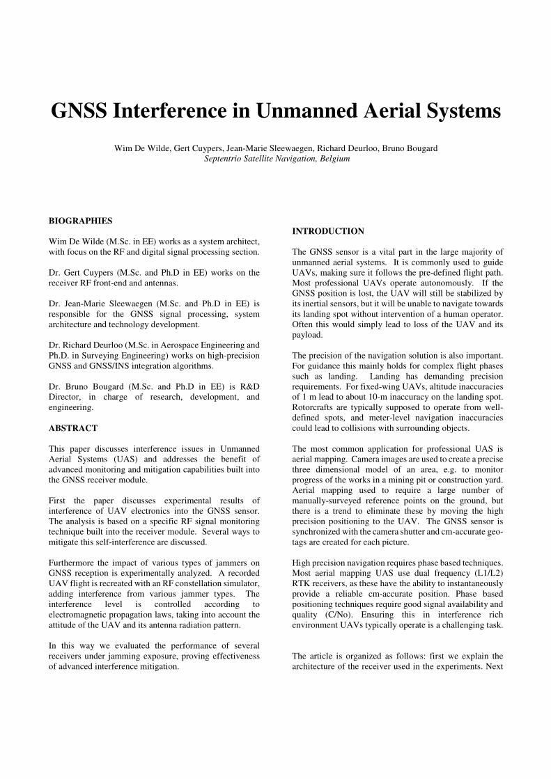
Figure 1: Septentrio’s AsteRx4 receiver architecture

This module is specifically designed for operation in harsh

interference environments. The antenna signal is down-

converted in a multi-channel two stage heterodyning front-

end with sharp surface acoustic wave (SAW) filters to

reject out-of-band interferers. The output signals are

quantized by multi-bit ADCs. The receiver has a built-in

capability to log a batch of raw RF signal. The logged

samples can be used to detect and study signal anomalies,

both in the time and frequency domain.

The digitized GNSS bands are automatically cleaned from

interference by multiple adaptive band-stop filters. Their

stop-band bandwidth is adjusted automatically between a

notch of a few kHz to a MHz-wide rejection, depending on

the nature of the interference.

The notch filters are complemented by an adaptive filter

capable to reject more complex types of interference such

as chirp jammers and frequency hopping interference like

DME/TACAN [1]. The receiver also supports regular

blanking [2, 3].

The sub-bands (GPS L1, L2, L5; GLONASS L1, L2;

GALILEO E1, E5; BeiDou B1, B2) are extracted by sub-

band filters, which isolate them from residual interference

in adjacent GNSS bands.

The recovered signals are further processed in a large

matrix of tracking channels, capable to simultaneously

process all satellite signals in all received bands, even after

the emerging constellations (e.g. GALILEO) will be

completed.

The collected measurements enter the navigation

processor, which computes a high-rate RTK, PPP or

SBAS-aided position depending on the corrections

provided to the receiver. The measurements can also be

logged onto flash memory (SD/eMMC) for replay or post

processing, along with the time tag of event-triggers. The

latter is particularly interesting for aerial geo-tagging

applications, as it eliminates the need to uplink differential

corrections to the UAV during the complete flight. RTK

accuracy can then be achieved by post-processing of the

logged GNSS measurements and photographs meta-data be

edited a posteriori.

SELF-INTERFERENCE

An important source of interference is the UAV itself. The

limited space available in UAVs causes the GNSS antenna

to be physically close to the on-board electrical and

electronic systems. This makes it vulnerable to

electromagnetic compatibility problems, which could

reduce overall receiver performance.

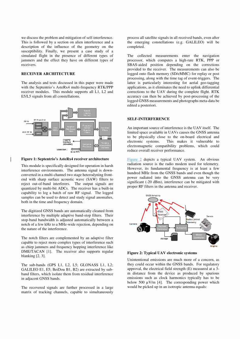
Figure 2 depicts a typical UAV system. An obvious

radiation source is the radio modem used for telemetry.

However, its fundamental frequency is at least a few

hundred MHz from the GNSS bands and even though the

power radiated into the GNSS antenna can be very

significant (-20 dBm), interference can be mitigated with

proper RF filters in the antenna and receiver.

Figure 2: Typical UAV electronic systems

Unintentional emissions are much more of a concern, as

they could occur within the GNSS bands. For regulatory

approval, the electrical field strength (E) measured at a 3-

m distance from the device as produced by spurious

emissions such as clock harmonics typically has to be

below 500 µV/m [4]. The corresponding power which

would be picked up in an isotropic antenna equals:

π

λ

4.

2

0

2

R

EP =

In which R0 is the free-space impedance of 377 ohm and

λ is the applicable wavelength. At the GPS L1

wavelength of 19 cm, this results into a power level of -87

dBm. This is far above the levels at which GNSS signals

start to show some level of degradation, which is between

-100 and -120 dBm, depending on the specific signal and

spectral location of the interference. In a UAV the GNSS

antenna is usually much closer than 3 m from the

electronics. This results in even higher field strengths,

even when taking into account that the antenna will provide

some rejection. Often the antenna will be exposed to near

field components.

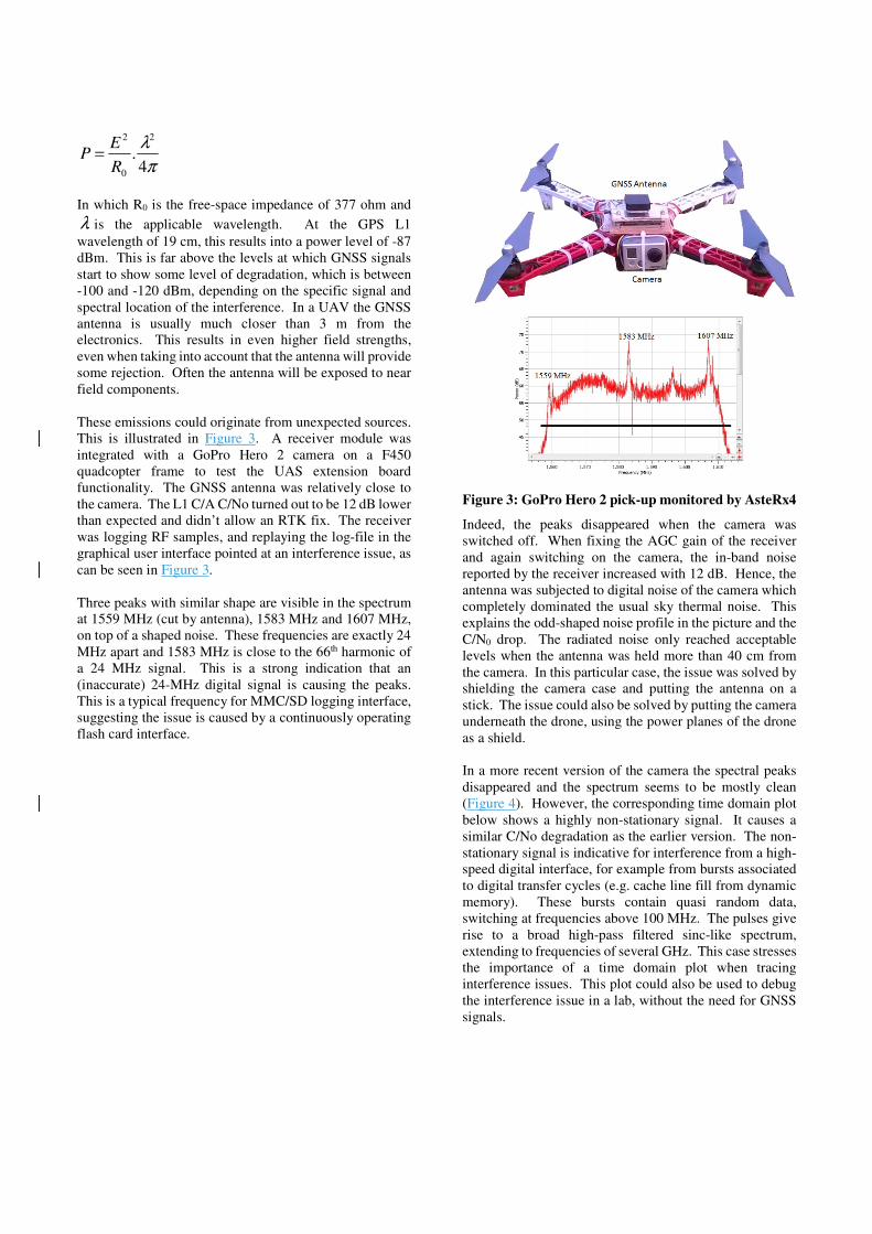
These emissions could originate from unexpected sources.

This is illustrated in Figure 3. A receiver module was

integrated with a GoPro Hero 2 camera on a F450

quadcopter frame to test the UAS extension board

functionality. The GNSS antenna was relatively close to

the camera. The L1 C/A C/No turned out to be 12 dB lower

than expected and didn’t allow an RTK fix. The receiver

was logging RF samples, and replaying the log-file in the

graphical user interface pointed at an interference issue, as

can be seen in Figure 3.

Three peaks with similar shape are visible in the spectrum

at 1559 MHz (cut by antenna), 1583 MHz and 1607 MHz,

on top of a shaped noise. These frequencies are exactly 24

MHz apart and 1583 MHz is close to the 66th harmonic of

a 24 MHz signal. This is a strong indication that an

(inaccurate) 24-MHz digital signal is causing the peaks.

This is a typical frequency for MMC/SD logging interface,

suggesting the issue is caused by a continuously operating

flash card interface.

Figure 3: GoPro Hero 2 pick-up monitored by AsteRx4

Indeed, the peaks disappeared when the camera was

switched off. When fixing the AGC gain of the receiver

and again switching on the camera, the in-band noise

reported by the receiver increased with 12 dB. Hence, the

antenna was subjected to digital noise of the camera which

completely dominated the usual sky thermal noise. This

explains the odd-shaped noise profile in the picture and the

C/N0 drop. The radiated noise only reached acceptable

levels when the antenna was held more than 40 cm from

the camera. In this particular case, the issue was solved by

shielding the camera case and putting the antenna on a

stick. The issue could also be solved by putting the camera

underneath the drone, using the power planes of the drone

as a shield.

In a more recent version of the camera the spectral peaks

disappeared and the spectrum seems to be mostly clean

(Figure 4). However, the corresponding time domain plot

below shows a highly non-stationary signal. It causes a

similar C/No degradation as the earlier version. The non-

stationary signal is indicative for interference from a high-

speed digital interface, for example from bursts associated

to digital transfer cycles (e.g. cache line fill from dynamic

memory). These bursts contain quasi random data,

switching at frequencies above 100 MHz. The pulses give

rise to a broad high-pass filtered sinc-like spectrum,

extending to frequencies of several GHz. This case stresses

the importance of a time domain plot when tracing

interference issues. This plot could also be used to debug

the interference issue in a lab, without the need for GNSS

signals.

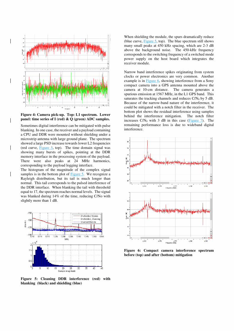
Figure 4: Camera pick-up. Top: L1 spectrum. Lower

panel: time series of I (red) & Q (green) ADC samples.

Sometimes digital interference can be mitigated with pulse

blanking. In one case, the receiver and a payload containing

a CPU and DDR were mounted without shielding under a

microstrip antenna with large ground plane. The spectrum

showed a large PSD increase towards lower L2 frequencies

(red curve, Figure 5, top). The time domain signal was

showing many bursts of spikes, pointing at the DDR

memory interface in the processing system of the payload.

There were also peaks at 24 MHz harmonics,

corresponding to the payload logging interface.

The histogram of the magnitude of the complex signal

samples is in the bottom plot of Figure 5. We recognize a

Rayleigh distribution, but its tail is much longer than

normal. This tail corresponds to the pulsed interference of

the DDR interface. When blanking the tail with threshold

equal to 17, the spectrum reaches normal levels. The signal

was blanked during 14% of the time, reducing C/No with

slightly more than 1 dB.

Figure 5: Cleaning DDR interference (red) with

blanking (black) and shielding (blue)

When shielding the module, the spurs dramatically reduce

(blue curve, Figure 5, top). The blue spectrum still shows

many small peaks at 450 kHz spacing, which are 2-3 dB

above the background noise. The 450-kHz frequency

corresponds to the switching frequency of a switched mode

power supply on the host board which integrates the

receiver module.

Narrow band interference spikes originating from system

clocks or power electronics are very common. Another

example is in Figure 6, showing interference from a Sony

compact camera into a GPS antenna mounted above the

camera at 10-cm distance. The camera generates a

spurious emission at 1567 MHz, in the L1 GPS band. This

saturates the tracking channels and reduces C/N0 by 5 dB.

Because of the narrow-band nature of the interference, it

could be mitigated with a notch filter in the receiver. The

bottom plot shows the residual interference using samples

behind the interference mitigation. The notch filter

increases C/N0 with 3 dB in this case (Figure 7). The

remaining performance loss is due to wideband digital

interference.

Figure 6: Compact camera interference spectrum

before (top) and after (bottom) mitigation

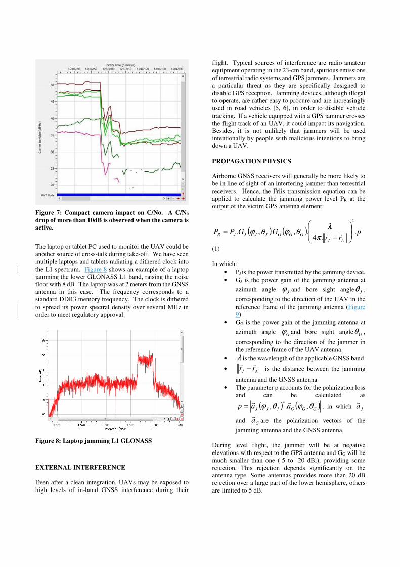
Figure 7: Compact camera impact on C/No. A C/N0

drop of more than 10dB is observed when the camera is

active.

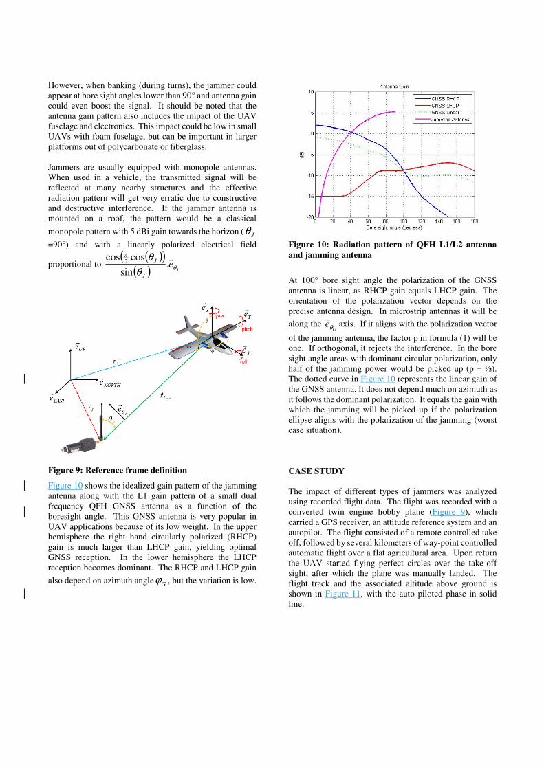
The laptop or tablet PC used to monitor the UAV could be

another source of cross-talk during take-off. We have seen

multiple laptops and tablets radiating a dithered clock into

the L1 spectrum. Figure 8 shows an example of a laptop

jamming the lower GLONASS L1 band, raising the noise

floor with 8 dB. The laptop was at 2 meters from the GNSS

antenna in this case. The frequency corresponds to a

standard DDR3 memory frequency. The clock is dithered

to spread its power spectral density over several MHz in

order to meet regulatory approval.

Figure 8: Laptop jamming L1 GLONASS

EXTERNAL INTERFERENCE

Even after a clean integration, UAVs may be exposed to

high levels of in-band GNSS interference during their

flight. Typical sources of interference are radio amateur

equipment operating in the 23-cm band, spurious emissions

of terrestrial radio systems and GPS jammers. Jammers are

a particular threat as they are specifically designed to

disable GPS reception. Jamming devices, although illegal

to operate, are rather easy to procure and are increasingly

used in road vehicles [5, 6], in order to disable vehicle

tracking. If a vehicle equipped with a GPS jammer crosses

the flight track of an UAV, it could impact its navigation.

Besides, it is not unlikely that jammers will be used

intentionally by people with malicious intentions to bring

down a UAV.

PROPAGATION PHYSICS

Airborne GNSS receivers will generally be more likely to

be in line of sight of an interfering jammer than terrestrial

receivers. Hence, the Friis transmission equation can be

applied to calculate the jamming power level PR at the

output of the victim GPS antenna element:

( ) ( ) prr

GGPPAJ

GGGJJJJR ..4

.,.,.

2

−= rr

π

λθϕθϕ

(1)

In which:

• PJ is the power transmitted by the jamming device.

• GJ is the power gain of the jamming antenna at

azimuth angle Jϕ and bore sight angle

Jθ ,

corresponding to the direction of the UAV in the

reference frame of the jamming antenna (Figure

9).

• GG is the power gain of the jamming antenna at

azimuth angle Gϕ and bore sight angle Gθ ,

corresponding to the direction of the jammer in

the reference frame of the UAV antenna.

• λ is the wavelength of the applicable GNSS band.

• AJ rrrr

− is the distance between the jamming

antenna and the GNSS antenna

• The parameter p accounts for the polarization loss

and can be calculated as

( ) ( )GGGJJJ aap θϕθϕ ,.,* rr

= , in which Jar

and Gar

are the polarization vectors of the

jamming antenna and the GNSS antenna.

During level flight, the jammer will be at negative

elevations with respect to the GPS antenna and GG will be

much smaller than one (-5 to -20 dBi), providing some

rejection. This rejection depends significantly on the

antenna type. Some antennas provides more than 20 dB

rejection over a large part of the lower hemisphere, others

are limited to 5 dB.

However, when banking (during turns), the jammer could

appear at bore sight angles lower than 90° and antenna gain

could even boost the signal. It should be noted that the

antenna gain pattern also includes the impact of the UAV

fuselage and electronics. This impact could be low in small

UAVs with foam fuselage, but can be important in larger

platforms out of polycarbonate or fiberglass.

Jammers are usually equipped with monopole antennas.

When used in a vehicle, the transmitted signal will be

reflected at many nearby structures and the effective

radiation pattern will get very erratic due to constructive

and destructive interference. If the jammer antenna is

mounted on a roof, the pattern would be a classical

monopole pattern with 5 dBi gain towards the horizon ( Jθ=90°) and with a linearly polarized electrical field

proportional to ( )( )

( ) Je

J

Jθ

π

θ

θ r.

sin

coscos2

Figure 9: Reference frame definition

Figure 10 shows the idealized gain pattern of the jamming

antenna along with the L1 gain pattern of a small dual

frequency QFH GNSS antenna as a function of the

boresight angle. This GNSS antenna is very popular in

UAV applications because of its low weight. In the upper

hemisphere the right hand circularly polarized (RHCP)

gain is much larger than LHCP gain, yielding optimal

GNSS reception. In the lower hemisphere the LHCP

reception becomes dominant. The RHCP and LHCP gain

also depend on azimuth angleGϕ , but the variation is low.

Figure 10: Radiation pattern of QFH L1/L2 antenna

and jamming antenna

At 100° bore sight angle the polarization of the GNSS

antenna is linear, as RHCP gain equals LHCP gain. The

orientation of the polarization vector depends on the

precise antenna design. In microstrip antennas it will be

along the G

eθ

raxis. If it aligns with the polarization vector

of the jamming antenna, the factor p in formula (1) will be

one. If orthogonal, it rejects the interference. In the bore

sight angle areas with dominant circular polarization, only

half of the jamming power would be picked up (p = ½).

The dotted curve in Figure 10 represents the linear gain of

the GNSS antenna. It does not depend much on azimuth as

it follows the dominant polarization. It equals the gain with

which the jamming will be picked up if the polarization

ellipse aligns with the polarization of the jamming (worst

case situation).

CASE STUDY

The impact of different types of jammers was analyzed

using recorded flight data. The flight was recorded with a

converted twin engine hobby plane (Figure 9), which

carried a GPS receiver, an attitude reference system and an

autopilot. The flight consisted of a remote controlled take

off, followed by several kilometers of way-point controlled

automatic flight over a flat agricultural area. Upon return

the UAV started flying perfect circles over the take-off

sight, after which the plane was manually landed. The

flight track and the associated altitude above ground is

shown in Figure 11, with the auto piloted phase in solid

line.

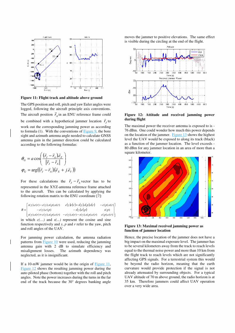
Figure 11: Flight track and altitude above ground

The GPS position and roll, pitch and yaw Euler angles were

logged, following the aircraft principle axis conventions.

The aircraft position Arr

in an ENU reference frame could

be combined with a hypothetical jammer location Jrr

to

work out the corresponding jamming power as according

to formula (1). With the conventions of Figure 9, the bore

sight and azimuth antenna angle needed to calculate GNSS

antenna gain in the jammer direction could be calculated

according to the following formulas:

( )

( )( )( )YXAJG

AJ

ZAJG

ejerr

rr

erra

rrrr

rr

rrr

..arg

.cos

+−=

−

−=

ϕ

θ

For these calculations the AJ rrrr

− vector has to be

represented in the XYZ-antenna reference frame attached

to the aircraft. This can be calculated by applying the

following rotation matrix to the ENU coordinate [7]:

( ) ( ) ( ) ( ) ( )( ) ( )

−−+

−−

−+−

=

)().()().().()().()().().()().(

)(.)().(

)().(..)().().()().(

rcpcrcpsysrsycrcpsycrsys

pspcyspcyc

rspcrspsysrcycrspsycrcys

R

in which c(…) and s(...) represent the cosine and sine

function respectively and y, p and r refer to the yaw, pitch

and roll angles of the UAV.

For jamming power calculation, the antenna radiation

patterns from Figure 10 were used, reducing the jamming

antenna gain with 2 dB to simulate efficiency and

misalignment losses. The azimuth dependency was

neglected, as it is insignificant.

If a 10-mW jammer would be in the origin of Figure 11,

Figure 12 shows the resulting jamming power during the

auto piloted phase (bottom) together with the roll and pitch

angles. Note the power increases during the turns in the far

end of the track because the 30° degrees banking angle

moves the jammer to positive elevations. The same effect

is visible during the circling at the end of the flight.

Figure 12: Attitude and received jamming power

during flight

The maximal power the receiver antenna is exposed to is -

76 dBm. One could wonder how much this power depends

on the location of the jammer. Figure 13 shows the highest

level the UAV would be exposed to along its track (black)

as a function of the jammer location. The level exceeds -

80 dBm for any jammer location in an area of more than a

square kilometer.

Figure 13: Maximal received jamming power as

function of jammer location

Hence, the precise location of the jammer does not have a

big impact on the maximal exposure level. The jammer has

to be several kilometers away from the track to reach levels

equal to the thermal noise power and more than 10 km from

the flight track to reach levels which are not significantly

affecting GPS signals. For a terrestrial system this would

be beyond the radio horizon, meaning that the earth

curvature would provide protection if the signal is not

already attenuated by surrounding objects. For a typical

UAV altitude of 70 m above ground, the radio horizon is at

35 km. Therefore jammers could affect UAV operation

over a very wide area.

TEST SETUP

In order to study the impact of jammers on UAVs, the flight

track discussed in the previous section was reproduced

with a Spirent L1/L2 GPS RF constellation simulator,

using recent GPS almanac data to define the constellation.

The radiation pattern of the QFH L1/L2 antenna was

modelled accurately to correctly simulate GPS power

during turns. The test also included a jamming source,

which was attenuated with a programmable attenuator to

bring it to the precomputed jamming level. This was

combined with the GPS signal from the simulator and the

resulting signal was provided to the receiver.

Figure 14 provides a more detailed overview of the test set-

up. The simulator signal was amplified with an external

LNA to simulate an active antenna. The interference

power was calibrated using the build-in spectrum analyzer

of the receiver, using the -174-dBm/Hz noise floor as a

reference. The simulator output was adjusted to match the

theoretical C/No values.

Figure 14: Interference simulation set-up

The simulator was providing RTCM data towards the

receiver, in order to let it achieve an RTK position fix.

It was important to precisely synchronize the attenuator

control with the simulation. For this the simulator’s

NMEA time tag was used as an index in a table with pre-

computed attenuation settings and the corresponding value

was immediately applied to the attenuator.

CHIRP JAMMERS

The impact of chirp jammers was analyzed to evaluate the

effectiveness of the adaptive filter in the AsteRx4 receiver.

These jammers output a sinewave within the GNSS bands

with rapidly changing frequency. Typical sweep periods

are in the order of 10 µs.

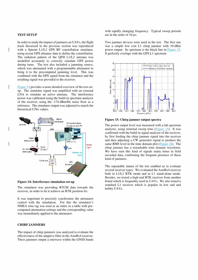
Two jammer devices were used in the test. The first one

was a simple low cost L1 chirp jammer with 10-dBm

power output. Its spectrum is the black line in Figure 15.

It perfectly overlaps with the GPS L1 spectrum

Figure 15: Chirp jammer output spectra

The power output level was measured with a lab spectrum

analyzer, using minimal sweep time (Figure 15). It was

confirmed with the build-in signal analyzer of the receiver,

by first feeding the chirp jammer signal into the receiver

and then adjusting a CW generator signal to produce the

same RMS level in the time domain plot (Figure 16). The

chirp jammer has a remarkable time domain waveform.

We have seen this kind of signals many times in field

recorded data, confirming the frequent presence of these

kind of jammers.

The repeatable nature of the test enabled us to evaluate

several receiver types. We evaluated the AsteRx4 receiver

both in L1/L2 RTK mode and in L1 stand-alone mode.

Besides, we tested a high-end RTK receiver from another

brand which is frequently used in UAVs. We also tested a

standard L1 receiver which is popular in low end and

hobby UAVs.

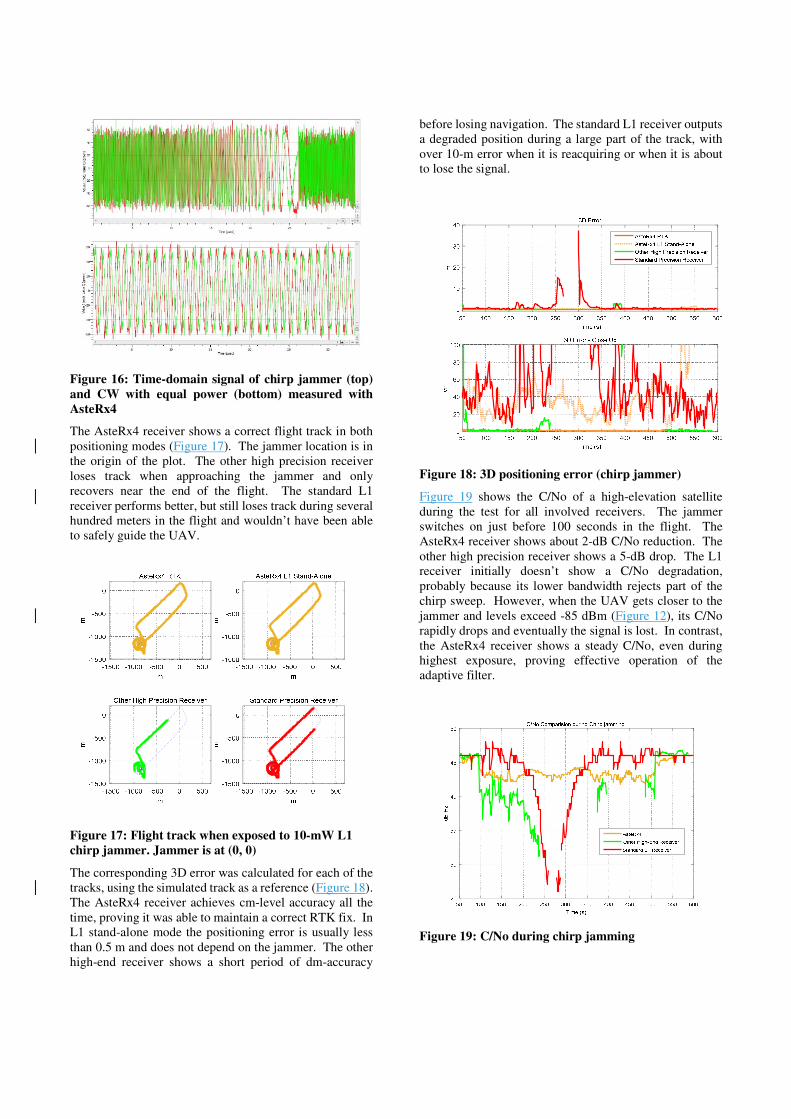
Figure 16: Time-domain signal of chirp jammer (top)

and CW with equal power (bottom) measured with

AsteRx4

The AsteRx4 receiver shows a correct flight track in both

positioning modes (Figure 17). The jammer location is in

the origin of the plot. The other high precision receiver

loses track when approaching the jammer and only

recovers near the end of the flight. The standard L1

receiver performs better, but still loses track during several

hundred meters in the flight and wouldn’t have been able

to safely guide the UAV.

Figure 17: Flight track when exposed to 10-mW L1

chirp jammer. Jammer is at (0, 0)

The corresponding 3D error was calculated for each of the

tracks, using the simulated track as a reference (Figure 18).

The AsteRx4 receiver achieves cm-level accuracy all the

time, proving it was able to maintain a correct RTK fix. In

L1 stand-alone mode the positioning error is usually less

than 0.5 m and does not depend on the jammer. The other

high-end receiver shows a short period of dm-accuracy

before losing navigation. The standard L1 receiver outputs

a degraded position during a large part of the track, with

over 10-m error when it is reacquiring or when it is about

to lose the signal.

Figure 18: 3D positioning error (chirp jammer)

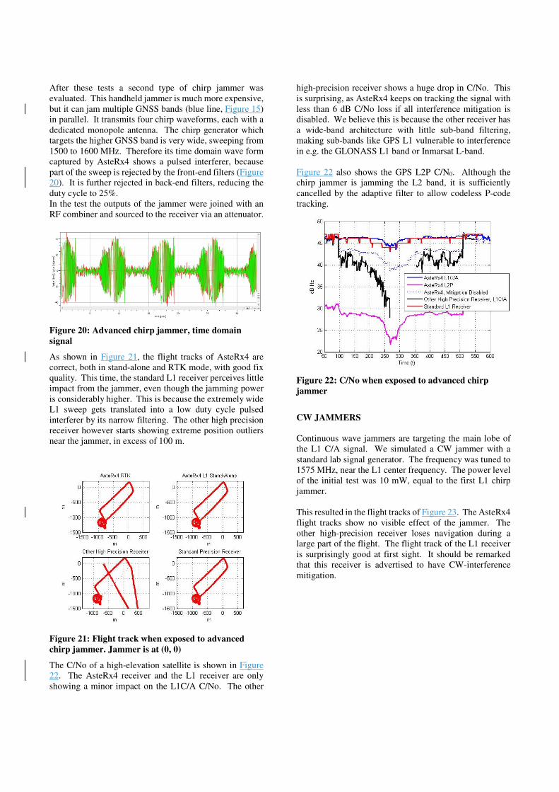
Figure 19 shows the C/No of a high-elevation satellite

during the test for all involved receivers. The jammer

switches on just before 100 seconds in the flight. The

AsteRx4 receiver shows about 2-dB C/No reduction. The

other high precision receiver shows a 5-dB drop. The L1

receiver initially doesn’t show a C/No degradation,

probably because its lower bandwidth rejects part of the

chirp sweep. However, when the UAV gets closer to the

jammer and levels exceed -85 dBm (Figure 12), its C/No

rapidly drops and eventually the signal is lost. In contrast,

the AsteRx4 receiver shows a steady C/No, even during

highest exposure, proving effective operation of the

adaptive filter.

Figure 19: C/No during chirp jamming

After these tests a second type of chirp jammer was

evaluated. This handheld jammer is much more expensive,

but it can jam multiple GNSS bands (blue line, Figure 15)

in parallel. It transmits four chirp waveforms, each with a

dedicated monopole antenna. The chirp generator which

targets the higher GNSS band is very wide, sweeping from

1500 to 1600 MHz. Therefore its time domain wave form

captured by AsteRx4 shows a pulsed interferer, because

part of the sweep is rejected by the front-end filters (Figure

20). It is further rejected in back-end filters, reducing the

duty cycle to 25%.

In the test the outputs of the jammer were joined with an

RF combiner and sourced to the receiver via an attenuator.

Figure 20: Advanced chirp jammer, time domain

signal

As shown in Figure 21, the flight tracks of AsteRx4 are

correct, both in stand-alone and RTK mode, with good fix

quality. This time, the standard L1 receiver perceives little

impact from the jammer, even though the jamming power

is considerably higher. This is because the extremely wide

L1 sweep gets translated into a low duty cycle pulsed

interferer by its narrow filtering. The other high precision

receiver however starts showing extreme position outliers

near the jammer, in excess of 100 m.

Figure 21: Flight track when exposed to advanced

chirp jammer. Jammer is at (0, 0)

The C/No of a high-elevation satellite is shown in Figure

22. The AsteRx4 receiver and the L1 receiver are only

showing a minor impact on the L1C/A C/No. The other

high-precision receiver shows a huge drop in C/No. This

is surprising, as AsteRx4 keeps on tracking the signal with

less than 6 dB C/No loss if all interference mitigation is

disabled. We believe this is because the other receiver has

a wide-band architecture with little sub-band filtering,

making sub-bands like GPS L1 vulnerable to interference

in e.g. the GLONASS L1 band or Inmarsat L-band.

Figure 22 also shows the GPS L2P C/N0. Although the

chirp jammer is jamming the L2 band, it is sufficiently

cancelled by the adaptive filter to allow codeless P-code

tracking.

Figure 22: C/No when exposed to advanced chirp

jammer

CW JAMMERS

Continuous wave jammers are targeting the main lobe of

the L1 C/A signal. We simulated a CW jammer with a

standard lab signal generator. The frequency was tuned to

1575 MHz, near the L1 center frequency. The power level

of the initial test was 10 mW, equal to the first L1 chirp

jammer.

This resulted in the flight tracks of Figure 23. The AsteRx4

flight tracks show no visible effect of the jammer. The

other high-precision receiver loses navigation during a

large part of the flight. The flight track of the L1 receiver

is surprisingly good at first sight. It should be remarked

that this receiver is advertised to have CW-interference

mitigation.

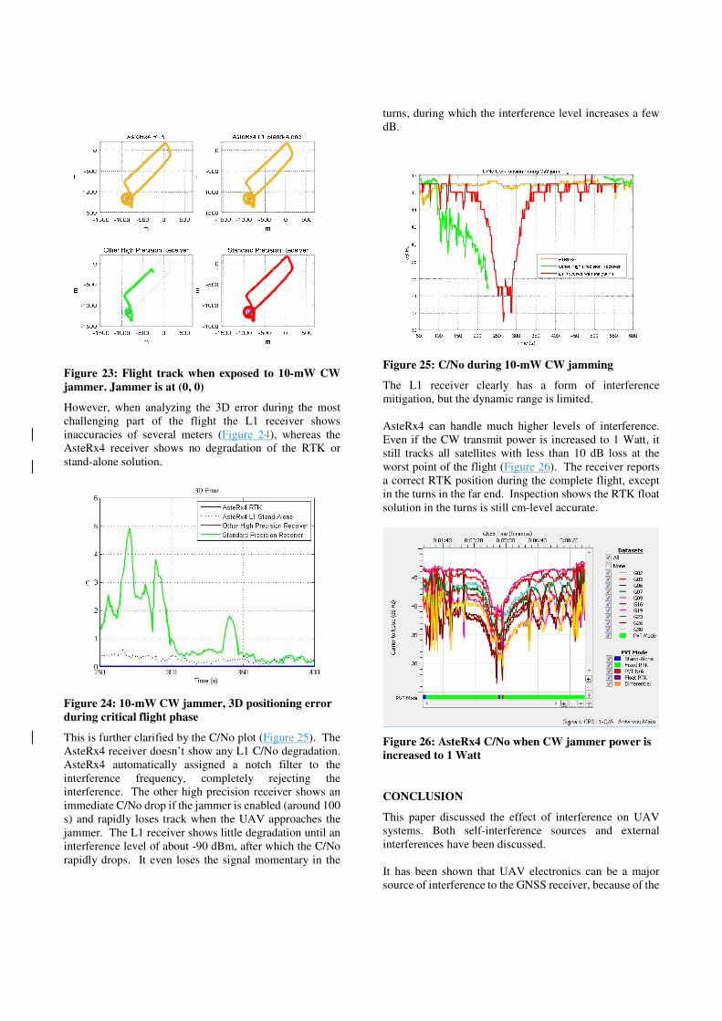
Figure 23: Flight track when exposed to 10-mW CW

jammer. Jammer is at (0, 0)

However, when analyzing the 3D error during the most

challenging part of the flight the L1 receiver shows

inaccuracies of several meters (Figure 24), whereas the

AsteRx4 receiver shows no degradation of the RTK or

stand-alone solution.

Figure 24: 10-mW CW jammer, 3D positioning error

during critical flight phase

This is further clarified by the C/No plot (Figure 25). The

AsteRx4 receiver doesn’t show any L1 C/No degradation.

AsteRx4 automatically assigned a notch filter to the

interference frequency, completely rejecting the

interference. The other high precision receiver shows an

immediate C/No drop if the jammer is enabled (around 100

s) and rapidly loses track when the UAV approaches the

jammer. The L1 receiver shows little degradation until an

interference level of about -90 dBm, after which the C/No

rapidly drops. It even loses the signal momentary in the

turns, during which the interference level increases a few

dB.

Figure 25: C/No during 10-mW CW jamming

The L1 receiver clearly has a form of interference

mitigation, but the dynamic range is limited.

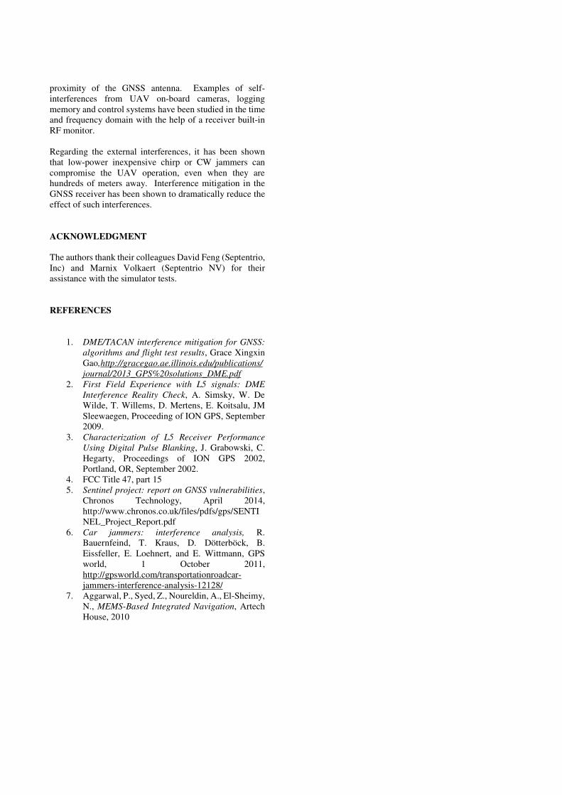
AsteRx4 can handle much higher levels of interference.

Even if the CW transmit power is increased to 1 Watt, it

still tracks all satellites with less than 10 dB loss at the

worst point of the flight (Figure 26). The receiver reports

a correct RTK position during the complete flight, except

in the turns in the far end. Inspection shows the RTK float

solution in the turns is still cm-level accurate.

Figure 26: AsteRx4 C/No when CW jammer power is

increased to 1 Watt

CONCLUSION

This paper discussed the effect of interference on UAV

systems. Both self-interference sources and external

interferences have been discussed.

It has been shown that UAV electronics can be a major

source of interference to the GNSS receiver, because of the

proximity of the GNSS antenna. Examples of self-

interferences from UAV on-board cameras, logging

memory and control systems have been studied in the time

and frequency domain with the help of a receiver built-in

RF monitor.

Regarding the external interferences, it has been shown

that low-power inexpensive chirp or CW jammers can

compromise the UAV operation, even when they are

hundreds of meters away. Interference mitigation in the

GNSS receiver has been shown to dramatically reduce the

effect of such interferences.

ACKNOWLEDGMENT

The authors thank their colleagues David Feng (Septentrio,

Inc) and Marnix Volkaert (Septentrio NV) for their

assistance with the simulator tests.

REFERENCES

1. DME/TACAN interference mitigation for GNSS:

algorithms and flight test results, Grace Xingxin

Gao,http://gracegao.ae.illinois.edu/publications/

journal/2013_GPS%20solutions_DME.pdf

2. First Field Experience with L5 signals: DME

Interference Reality Check, A. Simsky, W. De

Wilde, T. Willems, D. Mertens, E. Koitsalu, JM

Sleewaegen, Proceeding of ION GPS, September

2009.

3. Characterization of L5 Receiver Performance

Using Digital Pulse Blanking, J. Grabowski, C.

Hegarty, Proceedings of ION GPS 2002,

Portland, OR, September 2002.

4. FCC Title 47, part 15

5. Sentinel project: report on GNSS vulnerabilities,

Chronos Technology, April 2014,

http://www.chronos.co.uk/files/pdfs/gps/SENTI

NEL_Project_Report.pdf

6. Car jammers: interference analysis, R.

Bauernfeind, T. Kraus, D. Dötterböck, B.

Eissfeller, E. Loehnert, and E. Wittmann, GPS

world, 1 October 2011,

http://gpsworld.com/transportationroadcar-

jammers-interference-analysis-12128/

7. Aggarwal, P., Syed, Z., Noureldin, A., El-Sheimy,

N., MEMS-Based Integrated Navigation, Artech

House, 2010